Analysis of generalized Forchheimer flows of compressible fluids in porous media
47
ANALYSIS OF GENERALIZED FORCHHEIMER FLOWS OF COMPRESSIBLE FLUIDS IN POROUS MEDIA By Eugenio Aulisa Lidia Bloshanskaya Luan Hoang and Akif Ibragimov IMA Preprint Series # 2257 ( June 2009 ) INSTITUTE FOR MATHEMATICS AND ITS APPLICATIONS UNIVERSITY OF MINNESOTA 400 Lind Hall 207 Church Street S.E. Minneapolis, Minnesota 55455–0436 Phone: 612-624-6066 Fax: 612-626-7370 URL: http://www.ima.umn.edu
-
Upload
independent -
Category
Documents
-
view
3 -
download
0
Transcript of Analysis of generalized Forchheimer flows of compressible fluids in porous media
ANALYSIS OF GENERALIZED FORCHHEIMER FLOWS OF
COMPRESSIBLE FLUIDS IN POROUS MEDIA
By
Eugenio Aulisa
Lidia Bloshanskaya
Luan Hoang
and
Akif Ibragimov
IMA Preprint Series # 2257
( June 2009 )
INSTITUTE FOR MATHEMATICS AND ITS APPLICATIONS
UNIVERSITY OF MINNESOTA
400 Lind Hall207 Church Street S.E.
Minneapolis, Minnesota 55455–0436Phone: 612-624-6066 Fax: 612-626-7370
URL: http://www.ima.umn.edu
ANALYSIS OF GENERALIZED FORCHHEIMER FLOWS OFCOMPRESSIBLE FLUIDS IN POROUS MEDIA
EUGENIO AULISA, LIDIA BLOSHANSKAYA, LUAN HOANG AND AKIF IBRAGIMOV
Abstract. This work is focused on the analysis of non-linear flows of slightlycompressible fluids in porous media not adequately described by Darcy’s law.We study a class of generalized nonlinear momentum equations which coversall three well-known Forchheimer equations, the so-called two-term, power,and three-term laws. The non-linear Forchheimer equation is inverted to anon-linear Darcy equation with implicit permeability tensor depending on thepressure gradient. This results in a degenerate parabolic equation for the pres-sure. Two classes of boundary conditions are considered, given pressure andgiven total flux. In both cases they are allowed to be unbounded in time. Theuniqueness, Lyapunov and asymptotic stabilities, and other long-time dynami-cal features of the corresponding initial boundary value problems are analyzed.The results obtained in this paper have clear hydrodynamic interpretationsand can be used for quantitative evaluation of engineering parameters. Somenumerical simulations are also included.
Contents
1. Introduction 22. Formulation of the Problem 42.1. General Forchheimer equations 42.2. Boundary conditions 63. Non-Linear Darcy Equation and Monotonicity 74. Initial Boundary Value Problem and Uniqueness 145. Pseudo Steady State Solutions 176. Bounds for the Solutions 216.1. Solutions of IBVP-I type (S) 226.2. Solutions of IBVP-II type (S) 246.3. Comparing solutions of IBVP type (S) 267. Asymptotic Stability 298. Perturbed Boundary Value Problems 338.1. IBVP-I type (S) 338.2. IBVP-II type (S) 358.3. IBVP-I type (S) with flux constraints 399. Numerical Results 41References 44
Date: May 22, 2009.Key words and phrases. non-linear Darcy, generalized Forchheimer equations, porous media,
long-time dynamics, stability.
1

2 E. Aulisa, L. Bloshanskaya, L. Hoang, A. Ibragimov
1. Introduction
The mathematical modeling and analysis of non-linear flows in porous media isquickly becoming a key to solving many challenging problems in engineering andapplied sciences. Most of the studies in porous media are based on Darcy’s law,which describes a linear relationship between the pressure gradient and the fluidvelocity. “Darcy’s equation has become the model of choice for the study of the flowof fluids through porous solids due to pressure gradients, so much that it has nowbeen elevated to the status of a law in physics”[35]. However, almost immediatelyafter Darcy’s discovery, his student Dupuit observed on the field data that thislinear relation is no longer valid for flows with high values of velocity. Later,Forchheimer in his book [19] reported a number of experimental data underliningthese discrepancies, and constituted three different empirical formulae to interpretthese results. Nowadays researchers and engineers recognize that non-Darcy effectsare very important in many applications [41, 8, 24, 31, 32].
By analogy to pipe flows, it was originally assumed that “convective” forcesare responsible for non-linear deviations from laminar flow associated with Darcy’sequation. Later in the 1950s and 1960s (c.f. [10, 22] and references therein) it wasobserved that the Darcy law is valid as long as the Reynolds number (Re) does notexceed some characteristic value between 1 and 10. Unlike pipe flows, where thedeviation from linearity is associated with turbulence at high Re numbers, in porousmedia it occurs at low Re numbers. Yet, the actual nature of this phenomenon isnot fully understood. In recent experiments [38, 1] it was observed that in samplesof the porous media containing fractures Darcy’s law does not hold even for Re ≈ 1.The latest research suggests that even for low velocity flows, Darcy’s law needs tobe revised (see e.g. [9, 22]).
Almost all off-the-shelf industrial simulators of the process of filtration in porousmedia utilize the linear Darcy’s approximation of the momentum equation [40]. Inorder to capture physical phenomena lost in the linear approximation, researchershave been recently directed to the mathematical and numerical modeling of Forch-heimer flows, (c.f. [8, 17, 15, 26] and references therein). In those papers, the conti-nuity and the Forchheimer-Darcy’s momentum equations are treated separately as acoupled system of first order PDE. The Forchheimer equation can also be consideredas the limiting case of Brinkman-Forchheimer equations. There are a large numberof research on Brinkman-Forchheimer equations and Forchheimer equation in thisconnection with the former one for incompressible fluids [27, 28, 29, 30, 18, 39, 12].
A different approach to study analytically the long-time dynamics of the flowwas initiated in our previous works [3, 4, 7, 5, 6] for compressible fluids. Namely,to constitute a non-linear momentum equation with permeability tensor dependenton the pressure gradient. This leads to the reduction of the original system to onePDE for the pressure function only (see also [15]). Therefore ones can explore theequivalent problem within the framework of degenerate elliptic and parabolic PDE[20, 14].
In those papers, we mainly focus on the two-term Forchheimer law and the equi-librium states called pseudo-steady states (PSS). The PSS are defined by solutionsof auxiliary boundary value problems and are proved to be stable in the class ofsolutions of IBVP with constant total flux on the boundary. Also, the pressuregradient is assumed to be uniformly bounded for all time. The study there thenis used to analyze the productivity index/diffusive capacity in different industrial

Generalized Forchheimer Flows in Porous Media 3
problems. Those assumptions on the pressure are quite severe from theoretical andpractical points of view and leave much to be desired:
(a) Latest theoretical research (see [9]) indicates that even for low Reynoldsnumbers the pressure gradient can be a cubic function of the velocity. On the otherhand experimental and field data suggest different functional relations betweengradient of the pressure and velocity. Therefore there is a need to introduce ageneric Forchheimer law, which covers all polynomial dependence of the gradientof the pressure on the velocity.
(b) The above assumption on the boundedness of the pressure gradient ex-cludes sharp non-homogeneity in porous media, which often leads to deviation fromDarcy’s law (see [38, 1]).
(c) In practice, the production rate may vary in time and/or the pressure distri-bution on the well can become relatively large as time evolves (see [11]).
In the current paper, we investigate a class of general g-Forchheimer equationswhich cover all three classical Forchheimer laws, without any a priori assumptionon the hydrodynamic parameters (such as boundness of the pressure gradient).We prove that the g-Forchheimer equation is equivalent to non-linear Darcy equa-tion with permeability tensor K(·) depending on the pressure gradient. It is thenshown that the corresponding non-linear fieldK(y)y acquires important monotonic-ity properties. Moreover we introduce a class of g-Forchheimer equations consistingof generalized polynomials with positive coefficients (GPPC). For such equations,we show that for large |y| the non-linear permeability K(·) satisfies the followingasymptotic relation: K(y)y · y ≈ |y|(2−a), where a ∈ [0, 1) depends on the degree ofg-Forchheimer polynomial. Using these features, we develop a machinery to ana-lyze the behavior of non-linear hydrodynamic systems of Forchheimer type, dealingwith the change in physical parameters.
To model the regime of the filtration we consider two types of the boundaryconditions: given pressure or given total flux on the accessible boundary. To de-rive a priori estimates for the solutions to these IBVP, we introduce the functionH = H(x, t), defined in terms of the pressure gradient ∇p, whose integral playsthe role of a Lyapunov function. The L1 norm of H is equivalent to a “weightednorm” of |∇p|, and for the class of (GPPC) it is comparable with Sobolev normsof p(x, t) in W 1,q where q explicitly depends on the g-Forchheimer polynomial. Weinvestigate qualitative properties of the solutions and their long-time dynamics. Inparticular, the established monotonicity of the vector field K(y)y results in theLyapunov stability of the solutions. Moreover, the asymptotic stability is provedby utilizing the a priori estimates to balance the degeneracy of the parabolic equa-tion. Concerning the structural stability of the problems, we prove the continuousdependence of the solutions on the boundary data. This requires suitable traceestimates. We also obtain effective comparisons between solutions with two typesof boundary conditions: given pressure or given total flux.
Though problems discussed in this paper originate from hydraulic and reservoirengineering [10, 34], their mathematical studies may have wider applications. Forinstance, they can be adopted in biomathematics to investigate conjugate bloodflows in the lumen and arterial wall (see [2, 33] and references therein).
The paper is organized as follows:In Section 2 we introduce the generalized formulation of the Forchheimer’s laws
for slightly compressible fluids. Also, different boundary conditions are described,

4 E. Aulisa, L. Bloshanskaya, L. Hoang, A. Ibragimov
namely, the Dirichlet and the total flux boundary conditions. In Section 3, the re-sulting implicit non-linear Darcy equations are derived from the generalized Forch-heimer equations. Using those equations, the dynamics of the system can be de-scribed by a non-linear degenerate parabolic equation for the pressure only. Suchreduction is valid under the G-Conditions (see (3.3)). Primary properties of theequations are studied, particularly, the monotonicity under the Lambda-Condition(see (3.25)). We introduce the class of “generalized polynomials with positive coef-ficients” as the main model for our study and applications. In Section 4, two initialboundary value problems (IBVP) corresponding to two types of boundary condi-tions are introduced. The uniqueness and Lyapunov stability of their solutions arestudied. In Section 5, we focus on special time-dependent solutions, called pseudo-steady state solutions, which generate time-invariant velocity fields. Their a prioriestimates and Lipschitz continuity on the total flux are established. In Section6, we derive several a priori estimates for solutions of IBVP with boundary datasplit in time and spatial variables (see Definition 6.1). In Section 7, we obtain theasymptotic stability of the above IBVP. In Section 8, we study both IBVP withperturbed boundary data. We evaluate deviation between solutions with respectto deviation of the boundary data. In particular, we estimate their asymptoticdeviations. In Section 9, numerical computations are presented for different casesof generalized Forchheimer equations and boundary data to illustrate the precedingtheoretical study.
2. Formulation of the Problem
2.1. General Forchheimer equations. Darcy’s law is commonly related to vis-cous fluid laminar flows in porous media and is characterized by the permeabil-ity coefficient, which is obtained empirically in order to match the linear relationbetween velocity vector and pressure gradient. Darcy’s equation has also beenobtained rigorously within the context of homogenization and other averaging/up-scaling techniques [35, 37]. From hydrodynamic point of view, the Darcy’s equationis interpreted as the momentum equation. The Darcy’s equation, the continuityequation and the equation of state serve as the framework to model processes inreservoirs [25, 13]. For a slightly compressible fluid, the original PDE system re-duces to a scalar linear second order parabolic equation for the pressure only. Thepressure function is a major feature of the oil or gas filtration in porous media,which is bounded by the well surface and the exterior reservoir boundary. Differ-ent boundary conditions on the well correspond to different regimes of production,while the condition on the exterior boundary models flux or absence of flux intothe drainage area. All together, the linear parabolic equation, boundary conditionsand some assumptions or guesses about the initial pressure distribution form theIBVP.
There are different approaches for modeling non-Darcy’s phenomena [17, 19, 41,27, 36]. It can be derived from the more general Brinkman-Forchheimer’s equation[27, 12], or from mixture theory assuming certain relations between velocity fieldand “drag-like” forces due to fluid to solid friction in the porous media [35]. It canbe also derived using homogenization arguments [37], or assuming some functionalrelation and then match the experimental data. In the current paper we will justpostulate a general constitutive equation bounding the velocity vector field and thepressure gradient. We will introduce constraints on the momentum equation and
Generalized Forchheimer Flows in Porous Media 5
on the fluid density. This will allow the reduction of the original system to a scalarquasi-linear parabolic equation for the pressure only.
Hereafter, the following notation and basic definitions are used:
• u(x, t) is the velocity field; x ∈ Rd, d = 2, 3 spatial variable; t time; p(x, t)pressure distribution; y ∈ Rd variable vectors related to ∇p; s, ξ scalarvariables;
• Π dimensionless (normalized) permeability tensor - positive definite, sym-metric matrix; it may depend on spacial variable, and is subjected to con-ditions
(2.1) k1 ≥ (Π y, y)/|y|2 ≥ k0,
here (· , ·) is the scalar product in the Euclidean space, and |y| is the corre-sponding norm |y| = (
∑di=1 y
2i )1/2.
• The notations C,C0, C1, C2, . . . denote generic positive constants not de-pending on the solutions.
• When not specified, ‖ · ‖Lq and ‖ · ‖W r,q denote the norms over the domainU , i.e., ‖ · ‖Lq(U) and ‖ · ‖W r,q(U), respectively. Here the domain U ⊂ Rd ofinterest is fixed in the subsection 2.2 below.
In studies of flows in porous media, the three Forchheimer’s laws (two-term,power, and three-term) are widely used. Darcy and Forchheimer laws can be writtenin the vector forms as follows:
• The Darcy law
(2.2) αu = −Π∇p,
where α =µ
kwith k, in general, being the permeability non-homogeneous
function depending on x subjected to the condition: k−12 ≥ k ≥ k2,
1 ≥ k2 > 0. Here, the constant µ is the viscosity of the fluid.• The Forchheimer two-term law
(2.3) αu+ β√
(Bu, u)u = −Π∇p,
where β =ρFΦk1/2
, F is the Forchheimer’s coefficient, Φ is the porosity, andρ is the density of the fluid.
• The Forchheimer power law
(2.4) au+ cn√
(Bu, u)n−1u = −Π∇p,where n is a real number belonging to the interval [1, 2]. The strictlypositive and bounded functions c and a are found empirically, or can betaken as c = (n − 1)
√β and a = α. By this way, n = 1 and n = 2
reduce the power law (2.4) to Darcy’s law and to Forchheimer two-termlaw, respectively.
• The Forchheimer three-term law
(2.5) Au+ B√
(Bu, u)u+ C(Bu, u)u = −Π∇p.Here A,B, and C are empirical constants.
We now introduce a general form of Forchheimer equations.
6 E. Aulisa, L. Bloshanskaya, L. Hoang, A. Ibragimov
Definition 2.1 (g-Forchheimer Equations).
(2.6) g(x, |u|B)u = −Π∇p,here g(x, s) > 0 for all s ≥ 0 and |u|B =
√(Bu, u), where B = B(x) is a positive
definite tensor with bounded entries depending, in general, on the spatial variable.We will refer to (2.6) as g-Forchheimer (momentum) equations.
Under isothermal condition the state equation relates the density ρ = ρ(p) withthe pressure only. For slightly compressible fluid it takes the form:
(2.7)dρ
dp=
1κρ,
where 1/κ is the compressibility of the fluid. Substituting the last equation in thecontinuity equation
(2.8)dρ
dt= −∇ · (ρu),
yieldsdρ
dp
dp
dt= −ρ∇ · u− dρ
dpu · ∇p,
(2.9)dp
dt= −κ∇ · u− u · ∇p.
Since κ is large for most slightly compressible fluids in porous media, followingengineering tradition we drop the last term in (2.9) and study the reduced equation:
(2.10)dp
dt= −κ∇ · u .
2.2. Boundary conditions. Let U ⊂ Rd be a domain modeling the drainage areain the porous media (reservoir), bounded by two boundaries: the exterior boundaryΓe, and the accessible boundary Γi.
The exterior boundary Γe models the geometrical limit of the well impact onthe flow filtration and is often considered impermeable. This yields the boundarycondition:
(2.11) u ·N |Γe = 0,
where N is the outward normal vector on the boundary Γ = Γi ∪ Γe. Other typesof boundary conditions on the exterior boundary are discussed in [3].
The accessible boundary Γi models the well and defines the regime of filtrationinside the domain. On Γi the data are given rate of production Q(t), or givenpressure value p = ϕ(x, t), or a combination of both. It is very important froma practical point of view to build some “base line” solutions capturing significantfeatures of the well capacity and analyze the impact of the boundary conditions onthese solutions. This analysis will be used to forecast the well performances andtune the model to the actual data.
On the boundary Γi it is of particular interest the “split” condition of the fol-lowing type
(2.12) p = ψ(x, t) = γ(t) + ϕ(x),
where the time and space dependence of p are separated. This type of conditionmodels wells which have conductivity much higher than the conductivity inside the
Generalized Forchheimer Flows in Porous Media 7
reservoir. The limiting homogeneous case ψ(x) = const corresponds to the case ofinfinite conductivity on the well.
In case the flow is controlled by given production rate Q(t), the solution is notunique. We will restrict the class of solutions by imposing the split boundaryconstraint (2.12) on the well, where only ϕ(x) is known and γ(t) is determined byQ(t) (see Section 6).
Two important cases are:(a) pressure distribution of the form −At+ ϕ(x), and(b) constant total flux
∫Γiu ·Ndσ = Q = const.
The particular solutions of IBVP with boundary conditions (a) and (b) are “time-invariant” (see Section 5) and are used actively by engineers in their practical work.
3. Non-Linear Darcy Equation and Monotonicity
In order to make further constructions let the porous media be homogeneousand isotropic and the function g in (2.6) be independent of the spatial variables.Thus one has
(3.1) Π(x) = I, B(x) = I, g(x, |u|) = g(|u|),where I is the identity matrix. From (2.6) one has
(3.2) G(|u|) = g(|u|)|u| = |∇p|, where G(s) = sg(s), for s ≥ 0.
Henceforth in this section the following notation for function G and its inverseG−1 are used: G(s) = sg(s) = ξ, and s = G−1(ξ). To make sure one can solve (3.2)for |u|, we impose the following conditions.
G-Conditions: The function g belongs to C([0,∞)) and C1((0,∞)), and sat-isfies
(3.3) g(0) > 0, and g′(s) ≥ 0 for all s ≥ 0.
Under the G-Conditions, one has G′(s) = sg′(s) + g(s) ≥ g(0) > 0. Note alsoG(0) = 0. Hence G is a one-to-one mapping from [0,∞) onto [0,∞), therefore onecan find |u| as a function |∇p|(3.4) |u| = G−1(|∇p|)
Substituting equation (3.4) into (2.6) one obtains the following alternative formof the g-Forchheimer momentum equation (2.6):
Definition 3.1. (Non-linear Darcy Equation)
(3.5) u =−∇p
g(G−1(|∇p|)) = −K(|∇p|)∇p,
where the function K : [0,∞) → [0,∞) is defined by
(3.6) K(ξ) = Kg(ξ) =1
g(G−1(ξ)), ξ ≥ 0.
Note that
(3.7) G−1(0) = 0, K(0) =1g(0)
> 0.

8 E. Aulisa, L. Bloshanskaya, L. Hoang, A. Ibragimov
Substituting (3.5) for u into (2.10) one derives the degenerate parabolic equationfor the pressure:
(3.8)dp
dt= κ∇ · (K(|∇p|)∇p) .
Next, we will rewrite Eqs. (3.5) and (3.8) in their dimensionless form. Let 1/κ,Q and |U | be some reference values for the compressibility, the total production rateand the reservoir volume. Hence L = |U |1/d is the reference length and T = |U |/Qis the reference time. The dimensionless pressure and velocity p∗ and u∗ are definedas
(3.9) p∗ =p
κ,
(3.10) u∗ =Ld−1
Qu,
respectively. We also define the dimensionless nonlinear function
K∗(ξ∗) =κLd−2K(ξ)
Q=κLd−2K( κ
Lξ∗)
Q.
Eq. (3.5) can be rewritten as
(3.11)Q
Ld−1u∗ = −K(|∇∗ (κ/L p∗) |)∇∗(κ/L p∗),
or the same
(3.12) u∗ = −κLd−2K(|∇∗ (κ/L p∗) |)
Q∇∗p∗ = −K∗(|∇∗p∗|)∇∗p∗.
Similarly Eq. (3.8) can be rewritten as
(3.13)dp∗
dt∗=κLd−2K(|∇∗ (κ/L p∗) |)
Q∇∗p∗ = ∇∗ · (K∗(|∇∗p∗|)∇∗p∗) .
For sake of notation, we drop the ∗ apex, keeping in mind that all the quantitiesare dimensionless:
(3.14) u = −K(|∇p|)∇p,
(3.15)dp
dt= ∇ · (K(|∇p|)∇p) .
Some properties of the function K are stated in the following lemma.
Lemma 3.2. Let g(s) satisfy the G-Conditions.(i) The function K = Kg in (3.6) is well-defined, belongs to C1([0,∞)) and is
decreasing. Moreover, for any ξ ≥ 0, let s = G−1(ξ), then one has
(3.16) K ′(ξ) = −K(ξ)g′(s)
ξg′(s) + g2(s)≤ 0.
(ii) For any n ≥ 1, the function K(ξ)ξn is increasing and satisfies
(3.17) (K(ξ)ξn)′ = K(ξ)ξn−1
(n− ξg′(s)
ξg′(s) + g2(s)
)≥ 0, s = G−1(ξ).
(ii) The function y ∈ Rd → K(|y|)y belongs to C1(Rd \ {0}) and for y 6= 0
(3.18) ∇(K(|y|)y) = K(|y|)(I − g′(|y|)
|y|(|y|g′(s) + g2(s))y ⊗ y
),

Generalized Forchheimer Flows in Porous Media 9
where s = G−1(|y|).Proof. Eq. (3.16) follows from the chain rule
K ′(ξ) = − 1g2(s)
g′(s)1
G′(s)= −K(ξ)
g′(s)g(s)
1sg′(s) + g(s)
,
while Eq. (3.17) is obtained from (3.16) by direct substitution.For y ∈ Rd, y 6= 0, elementary calculations with the use of (3.16) give
(3.19)∂
∂yj(K(|y|)yi) = K(|y|)
(δij − g′(|y|)
|y|yiyj
|y|g′(s) + g2(s)
),
for i, j = 1, . . . , d, where s = G−1(|y|). This proves (3.19). ¤
It turns our that the function y → K(|y|)y associated with non-linear potentialfield on the RHS of equation (3.5) possesses a monotone property. This monotonic-ity and other monotone properties are crucial in the study of the uniqueness andqualitative behavior of the the solutions of initial value problems (see e.g. [16]).
Definition 3.3. Let F be a mapping from Rd to Rd.• F is monotone if
(3.20) (F (y′)− F (y)) · (y′ − y) ≥ 0, for all y′, y ∈ Rd.
• F is strictly monotone if there is c > 0 such that
(3.21) (F (y′)− F (y)) · (y′ − y) ≥ c|y′ − y|2, for all y′, y ∈ Rd.
• F is strictly monotone on bounded sets if for any R > 0, there is a positivenumber cR > 0 such that
(3.22) (F (y′)− F (y)) · (y′ − y) ≥ cR|y′ − y|2, for all |y′| ≤ R, |y| ≤ R.
To connect the above monotonicity and Eq. (3.5), we define the function Φ :Rd × Rd → R by
(3.23) Φ(y, y′) = (K(|y′|)y′ −K(|y|)y) · (y′ − y), for y, y′ ∈ Rd.
Proposition 3.4. Let g(s) satisfy the G-Conditions. Then F (y) = K(|y|)y ismonotone, hence
(3.24) Φ(y, y′) ≥ 0 for all y, y′ ∈ Rd.
The proof of Proposition 3.4 will be given below with that of Proposition 3.6.For stronger monotone properties, we impose an extra condition on g(s).Lambda-Condition: There is λ > 0 such that
(3.25) g(s) ≥ λsg′(s), for all s > 0.
Note that this condition is satisfied for any polynomial g(s) with positive coeffi-cients and positive exponents.
Lemma 3.5. Let g(s) satisfy the G-Conditions and the Lambda-Condition then
(3.26) 0 ≥ K ′(ξ) ≥ − 1λ+ 1
K(ξ)ξ
,
and
(3.27) (K(ξ)ξn)′ ≥ K(ξ)ξn−1
(n− 1
λ+ 1
)≥ 0 for n ≥ 1.
10 E. Aulisa, L. Bloshanskaya, L. Hoang, A. Ibragimov
Proof. Let s = G−1(ξ). If g′(s) = 0, then K ′(ξ) = 0 and one can easily verify thatinequalities (3.26) and (3.27) hold. We now assume g′(s) 6= 0. Inequality (3.26)follows by using Lambda-Condition (3.25) in (3.16)
K ′(ξ) = −K(ξ)g′(s)
ξg′(s) + g2(s)≥
−K(ξ)g′(s)
ξg′(s) + g(s)λsg′(s)= − 1
λ+ 1K(ξ)ξ
.
Inequality (3.27) follows at once from (3.26)
(K(ξ)ξn)′ = K ′(ξ)ξn + nK(ξ)ξn−1 ≥− 1λ+ 1
K(ξ)ξ
ξn + nK(ξ)ξn−1 = K(ξ)ξn−1
(n− 1
λ+ 1
)≥ 0
for n ≥ 1. ¤Proposition 3.6. Let g(s) satisfy the G-Conditions and the Lambda-Condition.Then F (y) = K(|y|)y is strictly monotone on bounded sets. More precisely,
(3.28) Φ(y, y′) ≥ λ
λ+ 1K(max{|y|, |y′|})|y′ − y|2, for all y, y′ ∈ Rd.
Proofs of Propositions 3.4 and 3.6. We consider the following two cases:Case 1: The origin does not belong to [y, y′]. Here [y, y′] is the line segment
connecting y and y′. Let z = y′ − y, and let γ(t) = (ty′ + (1 − t)y), t ∈ [0, 1], bethe parameterization of [y, y′]. Define h(t) = (K(|γ(t)|)γ(t)) · z, for t ∈ [0, 1].
By the Mean Value Theorem, there is t0 ∈ [0, 1] with y0 = γ(t0) 6= 0 such that
Φ(y, y′) = h(1)− h(0) = h′(t0) = (∇(K(|y0|)y0)(y′ − y)) · (y′ − y).
Recollecting identity (3.19) one gets:
Φ(y, y′) = K(|y0|)|y′ − y|2 −K(|y0|)g′(s)|y0|
∑i,j y0iy0j(y′j − yj)(y′i − yi)
|y0|g′(s) + g2(s)
= K(|y0|)|z|2 −K(|y0|)g′(s)|y0|
|y0 · z|2(|y0|g′(s) + g2(s))
,
where s = G−1(|y0|). Applying the Cauchy-Schwarz inequality to |y0 · z| yields
(3.29) Φ(y, y′) ≥ K(|y0|)|z|2(1− |y0|g′(s)
|y0|g′(s) + g2(s)
)≥ 0.
This proves (3.24).In case g(s) satisfies the Lambda-Condition, noting that |y0| = sg(s), one has
|y0|g′(s) + g2(s) ≥ |y0|g′(s) + g(s) (λsg′(s)) = |y0|g′(s) + λ|y0|g′(s).Hence
(3.30) Φ(y, y′) ≥ K(|y0|)|z|2(
1− |y0|g′(s)(1 + λ)|y0|g′(s)
)= K(|y0|)|z|2 λ
1 + λ.
Since |y0| is between |y| and |y′|, and K(·) is decreasing, the last inequalityimplies (3.28).
Case 2: The origin belongs to [y, y′]. We replace y′ by some yε 6= 0 so that0 6∈ [y, yε], and yε → 0 as ε→ 0. Apply the above inequality for y and yε, then letε→ 0.

Generalized Forchheimer Flows in Porous Media 11
Finally, (3.28) and the fact K is decreasing clearly imply that K(|y|)y is strictlymonotone on bounded sets. ¤
To illustrate the monotonicity properties, we consider the particular case of two-term Forchheimer’s equation. In this case function K can be calculated explicitly.
Example 3.7. For the Forchheimer two-term law (2.3), let g(s) = α + βs, then
one has G(s) = βs2 + αs and s = G−1(ξ) = −α+√
α2+4βξ
2β . Thus
K(ξ) =1
α+ βG−1(ξ)=
2
α+√α2 + 4βξ
.
One can easily verify that (3.25) holds with λ = 1. Proposition 3.4 then yields
Φ(y, y′) ≥ 12K(max{|y|, |y′|})|y′ − y|2.
The Lambda-Condition (3.25) imposes an exponential upper bound for g(s):
(3.31) g(s) ≤ A+Bs1/λ, ∀s ≥ 0, some A,B > 0.
It is not difficult to see that all three Forchheimer equations (2.3), (2.4), and (2.5)satisfies the G-conditions and Lambda-Condition. Based on those three models(2.3), (2.4), (2.5) and the constraint (3.31), we introduce the following “generalizedpolynomials with positive coefficients” (GPPC).
Definition 3.8. We say that a function g(s) is a GPPC if
(3.32) g(s) = a0sα0 + a1s
α1 + a2sα2 + . . .+ aks
αk =k∑
j=0
ajsαj ,
where k ≥ 0, the exponents satisfy 0 = α0 < α1 < α2 < . . . < αk, and thecoefficients a0, a1, . . . , ak are positive.
The largest exponent αk is the degree of g and is denoted by deg(g).Class (GPPC) is defined as the collection of all GPPC.
If the function g in Definition 2.1 belongs to class (GPPC) then we call it theg-Forchheimer polynomial.
Lemma 3.9. Let g(s) be a function of class (GPPC). Then g satisfies G-Conditionsand Lambda-Condition. Consequently, F (y) = Kg(|y|)y is strictly monotone onbounded sets and Ineq. (3.28) holds for K = Kg.
Proof. Obviously, g(s) satisfies the G-Conditions. We now check the Lambda-Condition. The case αk = 0, (3.25) holds trivially with any λ > 0. We consider thecase αk > 0. One has
sg′(s) =k∑
j=1
αjajsαj ≤ αk
k∑
j=1
ajsαj ≤ αk
k∑
j=0
ajsαj = αkg(s).
Thus the Lambda-Condition holds with λ = 1/αk. ¤
Lemma 3.10. Let g(s) be a function of class (GPPC) as in (3.32). Then K(ξ) =Kg(ξ) is well-defined, is decreasing and satisfies
(3.33)C0
(1 + ξ)a≤ K(ξ) ≤ C1
(1 + ξ)a, ∀ξ ≥ 0,
12 E. Aulisa, L. Bloshanskaya, L. Hoang, A. Ibragimov
where a = αk/(αk + 1) ∈ [0, 1), and C0 and C1 are positive numbers depending onaj’s and αj’s. Subsequently
(3.34) C2ξ2−a − 1 ≤ K(ξ)ξ2 ≤ C1ξ
2−a, ∀ξ ≥ 0,
where C2 = min(
C02 , 1
).
Proof. To prove inequalities in (3.33), one first notes that
ξ + 1 = sg(s) + 1 = 1 + a0s+ . . .+ aksαk+1 ≥ C3(1 + s)αk+1,
ξ + 1 = sg(s) + 1 = 1 + a0s+ . . .+ aksαk+1 ≤ C4(1 + s)αk+1,
andg(s) = a0 + . . .+ aks
αk ≤ C5(1 + s)αk ,
g(s) = a0 + . . .+ aksαk ≥ C6(1 + s)αk ,
where positive numbers C3 ,C4, C5 and C6 depend on coefficients aj ’s and αj ’s.Hence
K(ξ) =1g(s)
≥ 1C5(1 + s)αk
≥ 1C5[ 1
C 3(1 + ξ)]αk/(αk+1)
=C0
(1 + ξ)a,
and
K(ξ) =1g(s)
≤ 1C6(1 + s)αk
≤ 1C6[ 1
C 4(1 + ξ)]αk/(αk+1)
=C1
(1 + ξ)a.
To prove the left inequality in (3.34), one considers the two cases:
K(ξ)ξ2 ≥ 0 ≥ ξ2−a − 1, for ξ ≤ 1,
K(ξ)ξ2 ≥ C0ξ2
(1 + ξ)a≥ C0ξ
2
(2ξ)a=C0
2ξ2−a ≥ C0
2ξ2−a − 1, for ξ > 1,
which can be reduced to the left inequality in (3.34) for all ξ ≥ 0. To prove theright inequality in (3.34) one considers
K(ξ)ξ2 ≤ C1ξ2
(1 + ξ)a≤ C1ξ
2
ξa= C1ξ
2−a, ∀ξ ≥ 0 .
The proof is complete. ¤
As a consequence of the monotonicity, we have the following estimates whichwill be used repeatedly in the next sections.
Lemma 3.11. Let the function g be of the class (GPPC). For any functions f , p1
and p2, and for 1 ≤ q < 2, one has
(3.35)(∫
U
|f |qdx)2/q
≤ C
(∫
U1
K(|∇p1|) |f |2dx+∫
U2
K(|∇p2|) |f |2dx)
×{
1 + max(‖∇p1‖
Laq
2−q (U), ‖∇p2‖
Laq
2−q (U)
)}a
,
where
U1 = {x : |∇p1(x)| ≥ |∇p2(x)|}, U2 = {x : |∇p1(x)| < |∇p2(x)|}.
Generalized Forchheimer Flows in Porous Media 13
Consequently
(3.36)∫
U
Φ(∇p1,∇p2)dx ≥ C
(∫
U
|∇(p1 − p2)|qdx)2/q
×{
1 + max(‖∇p1‖
Laq
2−q (U), ‖∇p2‖
Laq
2−q (U)
)}−a
.
Proof. First,∫
U|f |qdx =
∫U1|f |qdx+
∫U2|f |qdx = J1 + J2, hence
(3.37)(∫
U
|f |qdx)2/q
≤ C(J2/q1 + J
2/q2 ).
By Holder inequality we have(3.38)
J1 =∫
U1
|f |qdx ≤(∫
U1
|f |qr · (K(|∇p1|))βrdx
) 1r
·(∫
U1
(K(|∇p1|))−βsdx
) 1s
,
where 1r + 1
s = 1 and β > 0 is a free parameter.By Lemma 3.10
(3.39)∫
U1
(K(|∇p1|))−βsdx ≤ C0
∫
U1
(1 + |∇p1|)βsadx ≤ C1(1 +∫
U1
|∇p1|βsadx) .
Set β r = 1, q r = 2, then
r =2q, β =
q
2, s =
22− q
, βs =q
2− q=s
r.
Hence it follows from (3.38) that
J2/q1 =
( ∫
U1
|f |pdx)2/q
≤(∫
U1
|f |2 ·K(|∇p1|)dx)C2
{1 +
(∫
U1
|∇p1|ap2−q dx
) 2−qq
}
≤ C3M
∫
U1
|f |2 ·K(|∇p1|)dx,
where M ={
1 + max(‖∇p1‖
Laq
2−q (U), ‖∇p2‖
Laq
2−q (U)
)}a
.
Similarly, one obtains the estimate for J2:
J2/q2 ≤ C4M
∫
U2
|f |2 ·K(|∇p2|)dx.
Combining the above estimates of J2/q1 and J2/q
2 with (3.37), one derives(∫
U
|f |qdx)2/q
≤ C5M( ∫
U1
|f |2 ·K(|∇p1|)dx∫
U2
|f |2 ·K(|∇p2|)dx)
which yields (3.35).To prove (3.36), one applies inequality (3.28) in Proposition 3.4 to have
(3.40)∫
U
Φ(∇p1,∇p2)dx ≥ λ
λ+ 1
[∫
U1
K(|∇p1|)|∇z|2dx+∫
U2
K(|∇p2|)|∇z|2dx],
where z = p1 − p2. Then apply Ineq. (3.35) with f = ∇z . ¤

14 E. Aulisa, L. Bloshanskaya, L. Hoang, A. Ibragimov
In our subsequent sections, we always assume that the function g(s) satisfies theG-Conditions. Therefore the function K(ξ) = Kg(ξ) and the equation (3.15) arewell-defined.
4. Initial Boundary Value Problem and Uniqueness
In this section we consider two IBVP for solutions of the equation (3.15). Theflow is subjected to the non-flow condition on exterior boundary Γe. On the accessi-ble boundary Γi, there are to two types of boundary conditions: (1) given pressuredistribution, and (2) given total flux. For general non-linear function g(s) satisfyingthe G-Conditions, we will prove the uniqueness of the IBVP for case (1) withoutany restriction, and for case (2) under additional constraint on the behavior of thesolutions on Γi. Furthermore, under the Lambda-Condition (3.25) on the functiong(s), we will show that solutions of both IBVP are asymptotically and exponen-tially stable (with respect to initial data), if the pressure gradients are bounded forall time.
We will study below two IBVP, namely, IBVP-I and IBVP-II, corresponding tothe Dirichlet and total flux conditions on Γi, respectively.
Definition 4.1. (IBVP-I) The function p(x, t) is a solution of the IBVP-I if p(x, t)satisfies:
(4.1)
∂p∂t = ∇ · (K(|∇p|)∇p) , in D = U × (0,∞),p(x, 0) = p0(x), in U,∂p∂N = 0 on Γe × (0,∞),p(x, t) = ψ(x, t) on Γi × (0,∞),
where p0(x) is the given the initial pressure, and ϕ(x, t) is the prescribed pressuredistribution on Γi.
Definition 4.2. (IBVP-II) The function p(x, t) is a solution of the IBVP-II ifp(x, t) satisfies:
(4.2)
dpdt = ∇ ·K(∇p)∇p, in D = U × (0,∞),p(x, 0) = p0(x), in U,∂p∂N = 0 on Γe × (0,∞),− ∫
ΓiK(∇p(x, t))∇p(x, t) ·N = Q(t) on Γi × (0,∞),
where p0(x) is the given initial pressure, and Q(t) is the prescribed total flux.
The solutions can be either the classical solutions or, more generally as studied inthis paper, the weak ones. For the latter class of solutions, one needs the followingassumptions:
• p(x, t) ∈ L2loc(0,∞;W 2,2(U)) and ∂p
∂t (x, t) ∈ L2loc(0,∞;W 1,2(U)),
• p(x, t) satisfies the first equation in (4.1) in the distributional sense,• p(x, t) satisfies the boundary conditions and initial data in the sense of
conventional traces.
We start with some primary properties of solutions of (3.15), which is the leadingdifferential equation in (4.1) and (4.2).

Generalized Forchheimer Flows in Porous Media 15
Lemma 4.3. Let pi(x, t), i = 1, 2 be two solution of the (3.15), satisfying im-permeable condition (2.10) on Γe. Let z(x, t) = p1(x, t) − p2(x, t) and functionΦ(∇p1,∇p2) be defined by (3.23). Then(4.3)12d
dt
∫
U
z2dx = −∫
U
Φ(∇p1,∇p2)dx+∫
Γi
z(K(|∇p1|)∇p1 −K(|∇p2|)∇p2) ·Ndσ,
(4.4)∫
U
|z(x, t)|2dx ≤∫
U
|z(x, 0)|2dx+2∫ t
0
∫
Γi
z(K(|∇p1|)∇p1 −K(|∇p2|)∇p2) ·Ndσdτ,
(4.5)∂
∂t
∫
U
zdx =∫
Γi
(K(|∇p1|)∇p1 −K(|∇p2|)∇p2) ·Ndσ,
(4.6)∫
U
z(x, t)dx =∫
U
z(x, 0)dx+∫ t
0
∫
Γi
(K(|∇p1|)∇p1 −K(|∇p2|)∇p2) ·Ndσdτ.
Proof. First observe that difference z(x, t) = p1(x, t)− p2(x, t) satisfies
(4.7)
{dzdt = ∇ · (K(|∇p1|)∇p1 −K(|∇p2|)∇p2),∂z∂N = 0 on Γe
By multiplying LHS and RHS of the equation (4.7) by z(x, t), integrating overdomain U , and applying Green’s formula to the RHS of the resulting equation, oneobtains identity (4.3).
Integrating (4.3) from 0 to t and using the monotonicity property (3.24), whichgives Φ(∇p1,∇p2) ≥ 0, one obtains inequality (4.4).
Next integrating the first equation in (4.7) over the domain, and applying theGreen formula to RHS yields (4.5), and consequently identity (4.6). ¤
Proposition 4.4. Let p1 and p2 are two solutions of IBVP-I (4.1). Then one hasfor all t ≥ 0 that
(4.8)∫
U
|p1(x, t)− p2(x, t)|2dx ≤∫
U
|p1(x, 0)− p2(x, 0)|2dx.
Subsequently, if p1(x, 0) = p2(x, 0) ∈ L2(U) then p1(x, t) = p2(x, t) for all t.Assume, in addition, that g(s) satisfies the Lambda-Condition (3.25), and
(4.9) ∇p1,∇p2 ∈ L∞(0,∞, L∞(U)).
Then
(4.10)∫
U
|p1(x, t)− p2(x, t)|2dx ≤ e−c1K(M)t
∫
U
|p1(x, 0)− p2(x, 0)|2dx,
for all t ≥ 0, where
(4.11) M = max{‖∇p1‖L∞(0,∞,L∞(U)), ‖∇p2‖L∞(0,∞;L∞(U))}.Consequently,
(4.12) limt→∞
∫
U
|p1(x, t)− p2(x, t)|2dx = 0.

16 E. Aulisa, L. Bloshanskaya, L. Hoang, A. Ibragimov
Proof. Let z(x, t) = p1(x, t) − p2(x, t). Since function z(x, t) vanishes on Γi, theintegral over the boundary Γi in (4.4) in the Lemma 4.3 is equal zero, and therefore
(4.13)∫
U
z2(x, t)dx ≤∫
U
z2(x, 0)dx.
Similarly we will obtain
(4.14)12d
dt
∫
U
z2dx = −∫
U
Φ(∇p1,∇p2)dx.
By the monotonicity (3.28), the fact that |∇p1|, |∇p2| ≤M , and the function K isdecreasing (Lemma 3.2), it follows that
(4.15) Φ(∇p1,∇p2) ≥ λ
1 + λK(M)|∇p1 −∇p2|2.
Then from (4.14) follows
(4.16)12d
dt
∫
U
z2dx ≤ −∫
U
λ
1 + λK(M)|∇z|2dx.
Applying Poincare’s inequality to RHS of the equation above one can get
(4.17)12d
dt
∫
U
z2dx ≤ −C λ
1 + λK(M)
∫
U
z2dx.
Finally using Gronwall’s inequality, we get (4.10). ¤
Proposition 4.5. Let p1 and p2 be two solutions of IBVP-II (4.2). Assume thedifference (p1 − p2) on Γi is independent of spatial variable x. Then
(4.18)∫
U
|p1(x, t)− p2(x, t)|2dx ≤∫
U
|p1(x, 0)− p2(x, 0)|2dx, t ≥ 0.
If g(s) satisfies the Lambda-Condition (3.25) and p1, p2 satisfy (4.9), then
(4.19)∫
U
|p1(x, t) − p2(x, t) − A0|2dx ≤ e−CK(M)t
∫
U
|p1(x, 0) − p2(x, 0) − A0|2dx,
for t ≥ 0, where A0 =∫
U(p1(x, 0)−p2(x, 0))dx, C > 0, and M is defined by (4.11).
Proof. Similar to Proposition 4.4, let z = p1 − p2. The function z(x, t) on Γi isspatially homogeneous, and total fluxes on the accessible boundary Γi for bothIBVP (4.2) are the same. Therefore, the integral over the boundary Γi in (4.3)becomes z(Q(t)−Q(t)) = 0. Hence one finds
(4.20)12d
dt
∫
U
z2dx = −∫
U
Φ(∇p1,∇p2)dx ≤ 0,
the last inequality is due to the monotonicity (3.24). Clearly, (4.18) and the unique-ness of the solution of IBVP-I (4.2) follow.
Next assume g(s) satisfies the Lambda-Condition. Let z = p1 − p2 − A0. Thefunction z solves (4.7), and hence equation (4.3) holds for z(x, t):(4.21)12d
dt
∫
U
z2dx = −∫
U
Φ(∇p1,∇p2)dx+∫
Γi
z(K(|∇p1|)∇p1 −K(|∇p2|)∇p2) ·Ndσ.
Generalized Forchheimer Flows in Porous Media 17
In addition, z(x, t) is spatially independent on the boundary Γi, and similar tothe above argument, the boundary term in (4.21) is equal to zero. Therefore (4.20)holds for function z:
(4.22)12d
dt
∫
U
z2dx = −∫
U
Φ(∇p1,∇p2)dx.
By virtue of Ineq. (3.28) in Proposition 3.6, we have
(4.23)12d
dt
∫
U
z2dx ≤ − λ
1 + λK(M)
∫
U
|∇z|2dx.
Applying Poincare inequality for RHS of the inequality (4.23) one gets
(4.24)12d
dt
∫
U
z2dx ≤ −12c1K(M)
∫
U
z2dx+ c1
(∫
U
zdx
)2
.
Since the total fluxes on Γi of both solutions are the the same, the integral overΓi in identity (4.6) is equal to zero. Therefore∫
U
z(x, t)dx =∫
U
z(x, 0)dx = 0.
Then estimate (4.19) follows from inequality (4.24) and Gronwall’s inequality.¤
Remark 4.6. As one can see from the above, the uniqueness for both IBVPfollows from simple monotonicity (3.20) of the vector field K(|∇p|)∇p, i.e. thenon-negativity of Φ(∇p1,∇p2). However asymptotic stability requires a strongercondition on K(|∇p|)∇p, provided by strict monotonicity on the bounded sets. Toguarantee this condition we imposed a constraint on the gradient of the solutionsto be bounded uniformly in time. This assumption is very restrictive. We will dropthis assumption in Sec. 7 for g belonging to class (GPPC), by utilizing the a prioriestimates of the pressure gradients in Sec. 6.
5. Pseudo Steady State Solutions
Often in engineering and physics it is essential to identify special time-dependentpressure distributions that generate flows which are time-invariant. In this sectionwe will introduce a class of the so-called pseudo-steady state (PSS) solutions whichis used frequently by reservoir and hydraulic engineers to evaluate “capacity” ofthe well (see. [3, 7, 21] and references therein).
Definition 5.1. A solution p(x, t) of the equation (3.15) in domain U , satisfyingthe Neumann condition on Γe is called the pseudo steady state (PSS) with respectto constant A if
(5.1)∂p(x, t)∂t
= const. = −A for all t.
Note: In practice, the constant A in the above definition is conventionally as-sumed to be positive. However, we will not impose that condition on A in ourstudy.
Equation (3.15) then reduces to
(5.2)∂p(x, t)∂t
= −A = ∇ · (K(|∇p|)∇p).
18 E. Aulisa, L. Bloshanskaya, L. Hoang, A. Ibragimov
Using Green’s formula and the Neumann boundary condition on Γe one derives
A|U | = −∫
Γi
(K(|∇p|)∇p) ·Ndσ =∫
Γi
u ·Ndσ = Q(t).
Therefore, the total flux of a PSS solution is time-independent
(5.3) Q(t) = A|U | = Q = const., for all t.
The PSS solutions inherit two important features of IBVP-I and IBVP-II, whichwe will explore further. On one hand, the total flux is defined by stationary equation(5.2) and is given. On the other hand, the trace of the solution on the boundary issplit a priori. Namely re-writing the PSS solution as
(5.4) p(x, t) = −At+ h(x),
one has ∇p = ∇h, hence h and p satisfy the same boundary condition on Γe. OnΓi, in general, we consider
(5.5) p(x, t) = −At+ ϕ(x), on Γi,
where ϕ(x) is given. Therefore h(x) satisfies
(5.6) −A = ∇ ·K(|∇h|)∇h,
(5.7)∂h
∂N= 0 on Γe,
(5.8) h = ϕ on Γi.
Of particular interest, we consider the case ϕ(x) = const. From physical pointof view, it relates to the constraint that conductivity inside well is non-comparablyhigher than in the porous media. By shifting the values of ϕ(x) and h(x) by aconstant, one has
(5.9) p(x, t) = −At+B +W (x),
where A and B are two numbers, and W (x) satisfies
(5.10) −A = ∇ ·K(|∇W |)∇W,
(5.11)∂W
∂N= 0 on Γe,
(5.12) W = 0 on Γi,
A solution h(x) of BVP (5.6), (5.7) and (5.8), considered in this study, is afunction in W 2,2(U) that satisfies (5.6) in the distributional sense and satisfies theboundary conditions (5.7) and (5.8) with its traces on Γ.
We call h(x) the profile of PSS corresponding to A and the boundary profileϕ(x). The solution W (x) of BVP (5.10), (5.11) and (5.12) is called the basic PSSprofile corresponding to A.
Remark 5.2. Note that for a PSS as in (5.4),
(5.13)1|U |
∫
U
p(x, t)dx− 1|Γi|
∫
Γi
p(x, t)dσ =1|U |
∫
U
h(x)dx− 1|Γi|
∫
Γi
ϕ(x)dσ,
that is, the difference between averages in the domain and on the boundary Γi
is independent of time. Engineers widely utilize this property in their routine to

Generalized Forchheimer Flows in Porous Media 19
calculate productivity index of the well, and sometimes use it as the definition ofPSS regime itself (see [3, 7, 21]). However we will not investigate the concept ofproductivity index for general g-Forchheimer flows in this article.
Proposition 5.3 (Uniqueness of PSS profile). Let the function g(s) satisfy theLambda-Condition (3.25).
(i) Then for each number A and boundary profile ϕ, there is at most one PSSprofile h(x) corresponding to A and ϕ(x).
(ii) Consequently, if p1 and p2 are two PSS solutions satisfying p1|Γi = p2|Γi
then p1(x, t) = p2(x, t) for all x ∈ U and t.
Proof. (i) Let h1, h2 be two solutions of the equation (5.6). Then by virtue of theboundary conditions, one has
0 =∫
U
(K(|∇h1|)∇h1 − F (|∇h2|)∇h2) · (∇h1 −∇h2)dx
≥ C
∫
U
K(|∇h1|+ |∇h2|)|∇h1 −∇h2|2dx.
The inequality above comes from Lemma 3.6. Since K(|∇h1(x)| + |∇h2(x)|) > 0a.e. one has ∇(h2(x)−h1(x)) = 0 a.e. in U . Therefore the fact that (h2−h1)|Γi = 0implies h2 − h1 = 0 in U .
(ii) Now, suppose pk(x, t) = −Akt + hk(x) and pk(x, t)|Γi = −Akt + ϕk(x) andp1 = p2 on Γi. Obviously, ϕ1(x) = ϕ2(x) and A1 = A2. Part (i) then impliesh1(x) = h2(x) and hence p1(x, t) = p2(x, t). ¤
We now focus on the study of the basic profile W (x). Applying Green’s formulato (5.10), one easily obtains the following identities:
(5.14) A = −∫
Γi
K(|∇W |)∇W ·Ndσ,
(5.15) A
∫
U
W (x)dx =∫
U
K(|∇W |)|∇W |2dx.
First, we derive an a priori estimate for W (x) with respect to constant A.
Theorem 5.4. Let the function g(s) be of class (GPPC) and a = deg(g)/(1 +deg(g)). Then for any number A, the corresponding basic profile W (x) satisfies
(5.16) ‖∇W‖L2−a(U) ≤ C (|A|+ 1)1/(1−a).
Proof. From (3.34) and (5.15) one can have∫
U
|∇W |2−adx ≤ C1
∫
U
K(|∇W |)|∇W |2dx+ C2 ≤ C1 ·A∫
U
|W |dx+ C2.
Applying Poincare inequality to RHS and the Young’s inequality we get
‖∇W‖2−aL(2−a) =
∫
U
|∇W |2−adx ≤ CA‖∇W‖L1 + C ≤ CA‖∇W‖L(2−a) + C
≤ ε‖∇W‖2−aL(2−a) + C|A|q + C,
where q = (2− a)/(1− a). Taking ε = 1/2 one obtains
‖∇W‖2−aL(2−a) ≤ C|A|q + C ≤ C(1 + |A|)q.
Then (5.16) follows. ¤

20 E. Aulisa, L. Bloshanskaya, L. Hoang, A. Ibragimov
Furthermore, basic profiles are continuous in A, hence in the total flux Q asshown below.
Theorem 5.5. Let g(s) be of class (GPPC). Let W1(x) and W2(x) be two basicprofiles corresponding A1 and A2, respectively. Then there exists a constant C suchthat
(5.17) ‖∇(W1 −W2)‖L2−a(U) ≤ CM |A1 −A2|,where a = deg(g)/(1 + deg(g)), M = (max(|A1|, |A2|) + 1)a/(1−a).
Consequently, for 1 ≤ q ≤ (2− a)∗ = d(2− a)/(d− (2− a)), one has
(5.18) ‖W1 −W2‖Lq(U) ≤ CM |A1 −A2|.Proof. Denote W = W1 −W2. Using (3.36), one has
(A2 −A1)∫
U
W (x)dx =∫
U
Φ(∇W2,∇W1)dx
≥ C
(∫
U
|∇W |pdx)2/p [
1 + max(‖∇W1‖
Lap
2−p, ‖∇W2‖
Lap
2−p
)]−a
.
Hence(∫
U
|∇W |pdx)2/p
≤ C|A2−A1|[1 + max
(‖∇W1‖
Lap
2−p, ‖∇W2‖
Lap
2−p
)]a∫
U
|W (x)|dx.
Let M1 = (|A1|+ 1)a/(1−a), M2 = (|A2|+ 1)a/(1−a) and M = max(M1, M2).We take p so that ap/(2− p) = 2− a which implies p = 2− a > 1. Therefore
(∫
U
|∇W |2−adx
)2/(2−a)
≤ CM |A2 −A1|∫
U
|W (x)|dx.
which yields
(5.19)(∫
U
|∇(W1 −W2)|2−adx
) 22−a
≤ CM |A1 −A2|∫
U
|W1 −W2|dx,
From (5.19) and Poincare inequality we have(∫
U
|∇W |2−adx
) 22−a
≤ CM |A1 −A2|∫
U
|W |dx
≤ CM |A1 −A2|(∫
U
|∇W |2−adx
) 12−a
,
hence yielding (5.17).Then (5.18) follows from (5.17) and Poincare-Sobolev’s inequality. ¤
Remark 5.6. The result obtained in Theorem 5.5 has a clear engineering interpre-tation and can be applied to evaluating the productivity index (PI) of a well. Toillustrate this point, suppose that the flow of slightly compressible fluid is subjectto g-Forchheimer momentum equation (2.6), and all assumptions used to deriveequation (3.15) hold. In previous work ([7]), productivity index of the well forpseudo-steady state regime with constant total rate Q is calculated as
(5.20) PI =Q|U |∫
UW (x)dx

Generalized Forchheimer Flows in Porous Media 21
It is clear in case of linear Darcy flow that the PI does not depend on rate Q.On contrary, the PI of non-linear Forchheimer flows depends on Q and this factmust be taken into account. The result in Theorem 5.5 allows ones to explicitlyestimate the PI of the well with respect to perturbation in Q. Let PI1 and PI2 areproductivity indices corresponding to Q1 = Q and Q2 = Q+ ∆Q, with “relatively”small ∆Q. Then we have
|PI1 − PI2| ≤ C(W,Q, |U |)|∆Q|.We will not study here applications of the developed framework to PI analysis,leaving this topic for a separate article.
6. Bounds for the Solutions
In the previous section we studied the PSS solutions which is reduced to (time-independent) elliptic BVP. Here we are investigating solutions of the (evolution)parabolic equations with two types of time-dependent boundary conditions. Namelywe will consider the IBVP with: (1) given pressure values (Dirichlet data) on Γi,and (2) given total flux on Γi. The second problem does not, in general, has aunique solution. Therefore we will restrain the boundary data to a certain class.We will derive a priori bounds for ∇p in appropriate Lq norms, where the exponentq explicitly depends on the degree of the function g. This study is important byitself and it will also be used in subsequent sections in the analysis of long-timedynamics of the non-linear process in porous media flows.
Consider a solution p(x, t) to either IBVP-I (4.1) or IBVP-II (4.2) as in Sec. 4.For our convenience, we recall the equations that p(x, t) satisfies
∂p
∂t= ∇ · (K(|∇p|)∇p), in U, t > 0,(6.1)
p(x, 0) = p0(x), in U,(6.2)∂p
∂N= 0 on Γe.(6.3)
For IBVP-I we study the following particular Dirichlet data on Γi:
(6.4) p(x, t) = γ(t) + ϕ(x) on Γi, t > 0,
where the function ϕ(x) is defined for x ∈ Γi and satisfies
(6.5)∫
Γi
ϕ(x)dσ = 0.
We call (γ(t), ϕ(x)) the boundary profile with temporal component γ(t) andspatial component ϕ(x).
We say that γ(t) is a PSS temporal profile if γ(t) = −At+B for some numbersA,B.
For IBVP-II, the total flux condition is
(6.6) −∫
Γi
K(|∇p|)∇p ·Nds = Q(t).
Note that the condition (6.5) is imposed to guarantee the uniqueness of thesplitting (6.4).

22 E. Aulisa, L. Bloshanskaya, L. Hoang, A. Ibragimov
By virtue of the boundary constraints (6.4) and (6.5) one has for t > 0 that
(6.7) γ(t) =1|Γi|
∫
Γi
γ(t)dσ =1|Γi|
∫
Γi
p(x, t)− ϕ(x)dσ =1|Γi|
∫
Γi
p(x, t)dσ.
The function γ(t) considered in this and next sections is assumed to satisfy:
(6.8) γ(t) ∈ C([0,∞)) and γ′(t) ∈ L2loc([0,∞)).
Definition 6.1. Depending on what data are available we classify the solutions asfollows.
• We say that p(x, t) is a solution of IBVP-I type (S), or IBVP-I(S), if itsatisfies (6.1), (6.2), (6.3), (6.4) and (6.5) with given p0(x), γ(t) and ϕ(x).
• We say that p(x, t) is a solution of IBVP-II type (S), or IBVP-II(S), if itsatisfies (6.1), (6.2), (6.3), and (6.6), with given p0(x) and Q(t); also thevalues of p(x, t) on Γi have the form (6.4) and (6.5), where γ(t) and ϕ(x)are not necessarily given.
• We say that p(x, t) is a solution of IBVP type (S), or IBVP-(S), if it isa solution of either IBVP-I(S) or IBVP-II(S).
6.1. Solutions of IBVP-I type (S). We will derive a priori estimate for solutionsof IBVP-I(S). The following function H(x, t) is used in the derivation.
Definition 6.2. For any function p(x, t) we define H[p](x, t) by:
(6.9) H[p](x, t) =∫ |∇p(x,t)|2
0
K(√s)ds,
for (x, t) ∈ U × [0,∞).
The function H[p] can be compared with |∇p| as follows.Claim: For any (x, t) one has
(6.10) K(|∇p(x, t)|)|∇p(x, t)|2 ≤ H[p](x, t) ≤ 2K(|∇p(x, t)|)|∇p(x, t)|2.Indeed, on one hand, the function K(
√s) is decreasing, by (3.16), hence one has
H[p](x, t) ≥∫ |∇p(x,t)|2
0
K(|∇p(x, t)|)ds = K(|∇p(x, t)|)|∇p(x, t)|2.
On the other hand, by setting the variable ξ =√s in (6.9) and using the in-
creasing property of K(ξ)ξ (see (3.17)) one has
H[p](x, t) =∫ |∇p(x,t)|
0
2ξK(ξ)dξ ≤∫ |∇p(x,t)|
0
2|∇p(x, t)|K(|∇p(x, t)|)ds
≤ 2K(|∇p(x, t)|)|∇p(x, t)|2.
Note: Also, the decrease of K(s) directly implies H[p](x, t) ≤ K(0)|∇p(x, t)|2.Moreover, if g(s) satisfies the Lambda-Condition then by Ineq. (6.10) above and
Ineq. (3.34) in Lemma 3.10, there are positive constants C0 and C1 such that
(6.11) C0|∇p(x, t)|2−a − 1 ≤ H[p](x, t) ≤ C1|∇p(x, t)|2−a.

Generalized Forchheimer Flows in Porous Media 23
Theorem 6.3. Let p(x, t) be a solution of IBVP-I(S) with the boundary profile(γ(t), ϕ(x)). Then one has for all t ≥ 0 that
(6.12)∫
U
K (|∇p(x, t)|) |∇p(x, t)|2 dx ≤ 2∫
U
K (|∇p(x, 0)|) |∇p(x, 0)|2 dx
+ |U |∫ t
0
(γ′(τ))2 dτ − 1|U |
∫ t
0
Q2(τ)dτ,
where Q(t) is defined by (6.6).If, in addition, g(s) belongs to class (GPPC), then one has
(6.13)∫
U
|∇p(x, t)|2−adx ≤ C1 + C2
∫
U
|∇p(x, 0)|2−adx
+ C3
∫ t
0
(γ′(τ))2 dτ − C4
∫ t
0
Q2(τ)dτ.
Proof. Multiply Eq. (6.1) by ∂p∂t and integrate over the domain U :
∫
U
(∂p
∂t
)2
dx = −∫
U
K(|∇p|)∇p · ∂∂t
(∇p)dx+∫
Γi
K(|∇p|)(∇p ·N)∂p
∂tds
= −∫
U
K(|∇p|)∇p · ∂∂t
(∇p)dx−Q(t) · γ′(t).(6.14)
Note that
(6.15) K(|∇p|)∇p · ∂∂t
(∇p) =12∂
∂t
∫ |∇p|2
0
K(√s)ds =
12∂
∂tH(x, t),
where H = H[p] defined by (6.9).Integrating Eq. (6.1) over U , one finds the relation
(6.16)d
dt
∫
U
p(x, t)dx =∫
U
∂P (x, t)∂t
dx = −Q(t).
By Holder’s inequality
(6.17) Q2(t) =(∫
U
∂p
∂tdx
)2
≤ |U |∫
U
(∂p
∂t
)2
dx.
It follows from (6.14), (6.15) and (6.17) that
(6.18)12
∫
U
∂
∂tH(t, x)dx = −
∫
U
(∂p
∂t
)2
dx− γ′(t) ·Q(t) ≤ −Q2(t)|U | − γ′(t) ·Q(t).
Applying Cauchy’s inequality to γ′(t) ·Q(t) we obtain
(6.19)12d
dt
∫
U
H(t, x)dx ≤ |U |2· |γ′(t)|2 − Q2(t)
2|U | ,
and thus
(6.20)∫
U
H(t, x)dx ≤∫
U
H(0, x)dx+ |U |∫ t
0
|γ′(τ)|2dτ − 1|U |
∫ t
0
Q2(τ)dτ.
Using (6.10) to estimate H(x, t) and H(x, 0) in (6.20), one obtains (6.12).On the other hand, using (6.11) instead of (6.10) in (6.20) yields (6.13). ¤

24 E. Aulisa, L. Bloshanskaya, L. Hoang, A. Ibragimov
6.2. Solutions of IBVP-II type (S). As a consequence of Proposition 4.5 inSec. 4, each solution of IBVP-II(S) is unique. Here we estimate
∫U|∇p(x, t)|2−adx
in terms of Q(t) but not γ(t).
Theorem 6.4. Let p(x, t) be a solution of IBVP-II(S) with total flux Q(t). Assumethat Q(t) ∈ C1([0,∞)). Then for any δ > 0, one has(6.21)∫
U
|∇p(x, t)|2−adx ≤ eδt
∫
U
|∇p(x, 0)|2−adx+∫ t
0
eδ(t−τ)(Λ∗(τ)− C1h2(τ)
)dτ,
for any t ≥ 0, where
(6.22) Λ∗(t) = C2L2 +C3|Q(t)| 2−a1−a +L0h0(t)+L1h1(t)+2h0(t)h1(t)+Cδh3(t),
the functions hi(t), i = 0, 1, 2, 3 are defined by
(6.23)h0(t) =
∫ t
0
|Q(τ)|dτ, h1(t) =∫ t
0
|Q′(τ)|dτ,
h2(t) =∫ t
0
Q2(τ)dτ, h3(t) =∫ t
0
|Q′(τ)| 2−a1−a dτ,
the positive numbers L0, L1, L2 depend on the initial data and are given by(6.24)
L0 = |Q(0)|, L1 =∣∣∣∫
U
p(x, 0)dx∣∣∣, L2 = 1 + L
2−a1−a
0 + L2−a1 +
∫
U
|∇p(x, 0)|2−adx,
and C1, C2, C3, Cδ are positive constants .
Proof. Let
(6.25) I(t) =12
∫
U
H(x, t)dx, J(t) =∫
U
|∇p(x, t)|2−adx.
By (6.11), one has
(6.26) C0(J(t)− 1) ≤ I(t) ≤ C1J(t).
From (6.18) above:
(6.27)d
dtI(t) ≤ −Q
2(t)|U | − γ′(t)Q(t).
Integrating this inequality from 0 to t and then integrating by parts the last termgive
(6.28) I(t)− I(0) ≤ −∫ t
0Q2(τ)dτ|U | − γ(t)Q(t) + γ(0)Q(0) +
∫ t
0
γ(τ)Q′(τ)dτ.
We need to estimate γ(t) in terms of Q(t). Using the formula of γ(t) in (6.7) andapplying Poincare’s inequality, one obtains
|γ(t)| ≤ C
∫
Γi
|p(x, t)|ds ≤ C
∫
U
|∇p(x, t)|dx+ C
∫
U
|p(x, t)|dx
≤ C
∫
U
|∇p(x, t)|dx+ C
(∫
U
|∇p(x, t)|dx+∣∣∣∣∫
U
p(x, t)dx∣∣∣∣).
Generalized Forchheimer Flows in Porous Media 25
Clearly from (6.16),∫
Up(x, t)dx =
∫Up(x, 0)dx − ∫ t
0Q(τ)dτ. Then one continues
the above estimate as
(6.29)|γ(t)| ≤ C
∫
U
|∇p(x, t)|dx+ C
∣∣∣∣∫
U
p(x, 0)dx∣∣∣∣ + C
∣∣∣∣∫ t
0
Q(τ)dτ∣∣∣∣
≤ CJ(t)1
2−a + C`1 + Ch0(t),
where `1 =∣∣∫
Up(x, 0)dx
∣∣ = L1.Combining this estimate of γ(t) with (6.28) and (6.26), one obtains
J(t) ≤ −Ch2(t) + C`2 + C(J(t)
12−a + `1 + h0(t)
)|Q(t)|
+ C
∫ t
0
(J(τ)
12−a + `1 + h0(τ)
)|Q′(τ)|dτ,
where `2 = I(0) + |γ(0)Q(0)|+ 1.Note that one can estimate |γ(0)| by using (6.29):
(6.30) |γ(0)| = limt↘0
|γ(t)| ≤ CJ(0)1
2−a + C`1,
and hence
`2 ≤ C(I(0) + |Q(0)|(J(0)1
2−a + `1) + 1) ≤ C(|Q(0)| 2−a1−a + I(0) + J(0) + `2−a
1 + 1).
This yields `2 ≤ C`3 where `3 = |Q(0)| 2−a1−a + J(0) + `2−a
1 + 1.Let δ > 0 be fixed. By Young’s inequality, one derives
J(t) ≤ −Ch2(t) + C`3 +(12J(t) + C|Q(t)| 2−a
1−a)
+ (`1 + h0(t))|Q(t)|
+∫ t
0
δJ(τ) + Cδ|Q′(τ)|2−a1−a dτ +
∫ t
0
(`1 + h0(τ))|Q′(τ)|dτ.
Therefore one obtains
(6.31) J(t) ≤ −Ch2(t) + δ
∫ t
0
J(τ)dτ + Λ∗(t).
where
(6.32)Λ∗(t) = C`3 + C|Q(t)| 2−a
1−a + (`1 + h0(t))|Q(t)|
+∫ t
0
(`1 + h0(τ))|Q′(τ)|dτ + Cδ
∫ t
0
|Q′(τ)| 2−a1−a dτ.
Note that
(6.33) `1|Q(t)| ≤ `2−a1 + |Q(t)| 2−a
1−a ,
(6.34) h0(t)|Q(t)| = h0(t)∣∣∣Q(0) +
∫ t
0
Q′(τ)dτ∣∣∣ ≤ h0(t)|Q(0)|+ h0(t)h1(t),
(6.35)∫ t
0
(`1 + h0(τ))|Q′(τ)|dτ ≤ `1h1(t) + h0(t)h1(t).
Hence Λ∗(t) ≤ Λ∗(t), where Λ∗(t) is defined by (6.22).Applying Gronwall’s inequality to (6.31) with Λ∗(t) replacing Λ∗(t) gives
J(t) ≤ J(0)eδt +∫ t
0
eδ(t−τ)(Λ∗(τ)− Ch2(τ)
)dτ,

26 E. Aulisa, L. Bloshanskaya, L. Hoang, A. Ibragimov
which yields Ineq. (6.21). ¤
6.3. Comparing solutions of IBVP type (S). The estimate in the Sec. 6.2 isadequate to establish the dependence of the solutions to IBVP-II(S) on the totalflux in finite time intervals (see Theorem 8.5 in Section 8.2 below). However, due toits exponential growth, it does not imply the asymptotic stability of the solutions.The estimate can be improved in some instances when additional information isprovided, for example, when a “related” solution p(x, t) of IBVP-I(S) is known,and the total flux has some monotone properties.
Here we will estimate a solution p(x, t) of IBVP-II(S) using a known solutionp(x, t) of IBVP-I(S) having the same total flux Q(t). The solution p(x, t) is calledbase line solution to IBVP-II(S) with respect to Q(t).
Theorem 6.5. Let g(s) be of class (GPPC). Let pγ(x, t) be a solution of IBVP-I(S)with known total flux Q(t) and known boundary profile (γ(t), ϕ(x)). Let p(x, t) be asolution of IBVP-II(S) with total flux Q(t) and boundary profile (B(t), ϕ(x)), whereB(t) is not given but bounded from above. Suppose that Q ∈ C1([0,∞)), Q′(t) ≥ 0and B(t) ≤ B0 <∞. Then
(6.36)∫
U
|∇p(x, t)|2−adx ≤ −C1h2(t) + C2
( ∫
U
|∇pγ(x, t)|2−adx+ |Q(t)| 2−a1−a
+ |Q(t)||γ(t)|)
+ C3L0,
where h2(t) is defined in (6.23) and(6.37)
L0 = 1+|B(0)−B0||Q(0)|+|B0|2−a+∫
U
|∇p(x, 0)|2−adx+∣∣∣∫
U
p(x, 0)−pγ(x, 0)dx∣∣∣2−a
.
Consequently,
(6.38)∫
U
|∇p(x, t)|2−adx ≤ −C4h2(t) + C5
( ∫ t
0
|γ′(τ)|2dτ + |Q(t)| 2−a1−a
+ |Q(t)||γ(t)|)
+ C6L1,
where
(6.39) L1 = L0 +∫
U
|∇pγ(x, 0)|2−adx.
Proof. Let I(t) and J(t) be defined as in (6.25). Applying (6.28) to the solutionp(x, t) with B(t) replacing γ(t), one has
I(t) ≤ I(0)− Ch2(t)−B(t)Q(t) +B(0)Q(0) +∫ t
0
B(τ) ·Q′(τ)dτ
≤ I(0)− Ch2(t)−B(t)Q(t) +B(0)Q(0) +∫ t
0
B0 ·Q′(τ)dτ= I(0)− Ch2(t) + (B0 −B(t))Q(t) + (B(0)−B0)Q(0).
Letting L2 = I(0) + |B(0)−B0||Q(0)|, one obtains
(6.40) I(t) ≤ CL2 − Ch2(t) + (|B0|+ |B(t)|)|Q(t)|.We now evaluate |B(t)| through γ(t),
∫U|∇p|2−adx. Applying the trace theorem
and then Poincare’s inequality, one gets
Generalized Forchheimer Flows in Porous Media 27
(6.41) |B(t)| = 1|Γi|
∣∣∣∣∫
Γi
p(x, t)dσ∣∣∣∣ ≤ C1
∫
U
|∇p|dx+ C2
∣∣∣∣∫
U
pdx
∣∣∣∣ .
Next, from Lemma 4.3 it follows that
(6.42)∣∣∣∣∫
U
p(x, t)dx∣∣∣∣ ≤
∣∣∣∣∫
U
pγ(x, t)dx∣∣∣∣ +
∣∣∣∣∫
U
(p(x, 0)− pγ(x, 0))dx∣∣∣∣ ≤ B1(t) + Z1,
where Z1 =∣∣∫
U(p(x, 0)− pγ(x, 0))dx
∣∣ and B1(t) =∫
U|pγ(x, t)|dx. Then
(6.43) |B(t)| ≤ C
∫
U
|∇p|dx+ CB1(t) + CZ1 ≤ CJ(t)1
2−a + CB1(t) + CZ1.
Combining this with (6.40) yields
(6.44) I(t) ≤ −Ch2(t) + C(J(t)1
2−a +B1(t) + L3)|Q(t)|+ CL2,
where L3 = Z1 + |B0|. Thus by Young’s inequality
(6.45) I(t) ≤ −Ch2(t) + εJ(t) + C|Q(t)| 2−a1−a + CB1(t)|Q(t)|+ CL4,
where L4 = L2 +L2−a3 . Then using Ineq. (6.26) and taking ε sufficiently small, one
obtains
(6.46) J(t) ≤ −Ch2(t) + C|Q(t)| 2−a1−a + CB1(t)|Q(t)|+ CL5,
where L5 = 1 + L4.To estimate B1(t), one uses Poincare-Sobolev inequality (e.g. [23], the space
W 1,2−a(U) is compactly embedded into L1(U)) and relation (6.7):
B1(t) ≤ C
∫
U
|pγ |dx ≤ C
(∫
U
|∇pγ |2−adx
) 12−a
+ C
∣∣∣∣∫
Γi
pγ(x, t)dσ∣∣∣∣
≤ C
(∫
U
|∇pγ |2−adx
) 12−a
+ C|γ(t)|.
Hence
(6.47) J(t) ≤ −Ch2(t) + C|Q(t)| 2−a1−a + C‖∇pγ‖L2−a |Q(t)|+ C|Q(t)||γ(t)|+ CL5.
Thus applying Young’s inequality to the third term on the RHS yields
(6.48)∫
U
|∇p(x, t)|2−adx ≤ −Ch2(t) + C
∫
U
|∇pγ(x, t)|2−adx+ C|Q(t)| 2−a1−a
+ C|Q(t)γ(t)|+ CL5.
Estimating L5 gives L5 ≤ CL0, hence (6.36) follows (6.48). Then utilizing estimate(6.13) for |∇pγ | in (6.36), one obtains (6.38). ¤
In case pγ(x, t) is a PSS solution, a sharper estimate is obtained below.
Theorem 6.6. Let g(s) belong to class (GPPC). Let p(x, t) be a solution of IBVP-II(S) with total flux Q(t) ≡ Q = const., with the boundary profile (B(t), ϕ(x))
28 E. Aulisa, L. Bloshanskaya, L. Hoang, A. Ibragimov
satisfying ϕ(x) = 0. Assume the basic PSS profile W (x) corresponding to Q/|U |exists. Then there is a positive constant C such that for all t ≥ 0 one has
(6.49)∫
U
K(|∇p(x, t)|)|∇p(x, t)|2dx ≤ C(1 +
∫
U
K(|∇p(x, 0)|)|∇p(x, 0)|2dx
+∫
U
K(|∇W (x)|)|∇W (x)|2dx),
or equivalently,
(6.50)∫
U
|∇p(x, t)|2−adx ≤ C
(1 +
∫
U
|∇p(x, 0)|2−adx+∫
U
|∇W (x)|2−adx
).
Consequently,
(6.51)∫
U
|∇p(x, t)|2−adx ≤ C
(1 +
∫
U
|∇p(x, 0)|2−adx+ |Q| 2−a1−a
).
Proof. Let γ(t) = −tQ/|U | and let pγ(t) = γ(t) +W (x) be the corresponding PSSsolution with the total flux Qγ(t) = Q(t) = Q.
As in the proof of Lemma 6.5, one has
0 ≤∫
U
(∂tp− ∂tpγ)2dx = −∫
U
(K(|∇p|)∇p−K(|∇pγ |)∇pγ) · (∂t∇p− ∂t∇pγ)dx
+∫
Γi
(K(|∇p|)∇p−K(|∇pγ |)∇pγ) ·N(∂tp− ∂tpγ)dσ.
One easily gets
(6.52)
0 ≤ −∫
U
(K(|∇p|)∇p · ∂t∇pdx−∫
U
K(|∇pγ |)∇pγ · ∂t∇pγdx
+∫
U
(K(|∇p|)∇p · ∂t∇pγdx+∫
U
K(|∇pγ |)∇pγ · ∂t∇pdx+ (B′(t)− γ′(t)) (Qγ(t)−Q(t)).
Note that ∇pγ = ∇W and ∂t∇pγ = 0. Let H(x, t) = H[p](x, t) and Hγ(x, t) =H[pγ ](x, t) be defined as in (6.9). Then
0 ≤ −12∂t
∫
U
Hdx− 0 + 0 + ∂t
∫
U
K(|∇W |)∇W · ∇pdx+ 0
= −12∂t
∫
U
H(x, t)dx+ ∂t
∫
U
K(|∇W |)∇W · ∇pdx.
Integrating this inequality from 0 to t, we obtain
12
∫
U
H(x, t)dx ≤ 12
∫
U
H(x, 0)dx+∫
U
K(|∇W |)∇W · ∇p(x, t)dx
−∫
U
K(|∇W |)∇W · ∇p(x, 0)dx.
Generalized Forchheimer Flows in Porous Media 29
Applying Lemma 3.10 to function H(x, t) in LHS of the inequality above andYoung’s inequality with to the term K(|∇W |)∇W · ∇p, one gets
12
∫
U
K(|∇p|)|∇p|2dx ≤∫
U
K(|∇p(x, 0)|)|∇p(x, 0)|2dx
+ ε
∫
U
|∇p|2−adx+ C
∫
U
|∇p(x, 0)|2−adx+ C
∫
U
|K(|∇W |)∇W |) 2−a1−a dx.
By (3.34), one finally obtains
12
∫
U
K(|∇p|)|∇p|2dx ≤ C
∫
U
K(|∇p(x, 0)|)|∇p(x, 0)|2dx+ ε
∫
U
K(|∇p|)|∇p|2dx
+ C
∫
U
(|∇W |1−a)2−a1−a dx+ C
≤ Cε
∫
U
K(|∇p|)|∇p|2dx+ C
∫
U
K(|∇p(x, 0)|)|∇p(x, 0)|2dx
+ C
∫
U
K(|∇W (x)|)|∇W (x)|2dx+ C.
Letting ε be sufficiently small, one obtains (6.49). With (6.50), one uses (3.34)again to obtain (6.50).
The Ineq. (6.51) simply follows (6.50) and the estimate (5.16) of the solution Win Section 5. ¤
As a consequence, we obtain an improvement of Theorem 6.3 for the special caseof PSS boundary profile.
Corollary 6.7. Let p(x, t) be a solution to IBVP-I(S) with the PSS boundaryprofile, i.e., the boundary profile (B(t), ϕ(x)) satisfies B′(t) = −A and ϕ(x) = 0.Assume that the basic PSS solution corresponding to A exists. Then one has forany t ≥ 0 that
(6.53)∫
U
|∇p(x, t)|2−adx ≤ C
(1 +
∫
U
|∇p(x, 0)|2−adx+ |A| 2−a1−a
).
Proof. Proceed as in the proof of Theorem 6.6. Note that the last term in (6.52)vanishes because B′(t) = γ′(t) = −A. We omit the details. ¤
7. Asymptotic Stability
In this section we study the stability of IBVP-I(S) and IBVP-II(S). Their Lya-punov stability is already a consequence of Propositions 4.4 and 4.5 in Section 4.
Theorem 7.1. The IBVP-I(S) and IBVP-II(S) are Lyapunov stable with respectto the L2 norm. More specifically, if p1 and p2 are two solutions of the sameIBVP-(S), then
(7.1) ‖p1(·, t)− p2(·, t)‖L2(U) ≤ ‖p1(·, 0)− p2(·, 0)‖L2(U),
for all t ≥ 0.
We now focus on the asymptotic stability. For this, unlike the Lyapunov stabilityin Theorem 7.1, the nonlinear function g(s) will be restricted to the class (GPPC).
Let us start with notations and assumptions used henceforward:

30 E. Aulisa, L. Bloshanskaya, L. Hoang, A. Ibragimov
The function g(s) belongs to class (GPPC), a = deg(g)/(1 + deg(g)) and b =a/(2− a).
Two solutions pk(x, t), (k = 1, 2), of IBVP-(S) have boundary profiles (γk(t), ϕk(x)),and the total flux Qk(t), with ϕ1(x) = ϕ2(x) = ϕ(x).
For simplicity, we assume that
(7.2) γk(t), Qk(t) ∈ C1([0,∞)), k = 1, 2.
The difference of two solutions is z(x, t) = p1(x, t)− p2(x, t).The differences of boundary data are denoted by:
(7.3)∆γ(t) = γ1(t)− γ2(t), ∆′
γ(t) = γ′1(t)− γ′2(t),
∆Q(t) = Q1(t)−Q2(t), ∆′Q(t) = Q′1(t)−Q′2(t).
We will establish various estimates for∫
Uz2(x, t)dx for t ≥ 0 under different
boundary conditions.First, we derive a general differential inequality which will be applied to different
scenarios both in this section and the next one.
Lemma 7.2. One has for all t ≥ 0,
(7.4) 12d
dt
∫
U
z2(x, t)dx ≤ −C[∫
U
|∇z(x, t)|qdx] 2
q
N(t)−b −∆γ(t)∆Q(t),
where 1 ≤ q ≤ 2− a and
(7.5) N(t) = 1 +∫
U
|∇p1(x, t)|2−adx+∫
U
|∇p2(x, t)|2−adx.
Proof. First, one easily derives
12d
dt
∫
U
z2dx = −∫
U
Φ(∇p1,∇p2)dx−∆γ(t)∆Q(t).(7.6)
Then applying Ineq. (3.36) yields
12d
dt
∫
U
z2dx
≤ −C[∫
U
|∇z|qdx] 2
q
[1 + max(‖∇p1‖Lap/(2−p) , ‖∇p2‖Lap/(2−p))]−a −∆γ(t)∆Q(t)
≤ −C[∫
U
|∇z|qdx] 2
q [1 + ‖∇p1‖2−a
L2−a + ‖∇p2‖2−aL2−a
] −a2−a −∆γ(t)∆Q(t).
which proves Ineq. (7.4). Above, we imposed the condition
¤(7.7) aq/(2− q) ≤ 2− a, which is equivalent to, q ≤ 2− a.
As usual, we start with IBVP-I.
Theorem 7.3. Assume that deg(g) ≤ 4d−2 . Suppose p1(x, t), p2(x, t) are two
solutions of IBVP-I(S) with the same boundary profile (γ(t), ϕ(x)). Then(7.8)
‖p1(x, t)− p2(x, t)‖L2(U) ≤ ‖p1(x, 0)− p2(x, 0)‖L2(U) · exp[−C
∫ t
0
Λ−b(τ)dτ],
Generalized Forchheimer Flows in Porous Media 31
for all t ≥ 0, where
Λ(t) = 1 +∫
U
|∇p1(x, 0)|2−adx+∫
U
|∇p2(x, 0)|2−adx+∫ t
0
|γ′(τ)|2dτ.
Proof. First, N(t) in (7.5) can be bounded by using the estimate (6.13) for eachsolution p1, p2:
(7.9) N(t) ≤ CΛ(t).
Then apply Lemma 7.2 with γ1(t) = γ2(t) = γ(t) and use (7.9), one gets
(7.10) 12d
dt
∫
U
z2dx ≤ −C[∫
U
|∇z|qdx] 2
q
Λ(t)−a
2−a ,
where C is independent of the solutions p1 and p2.Further we apply Sobolev’s inequality (e.g. [23]) to function z with z|Γi
= 0 tohave:
(7.11)∫
U
z2dx ≤ C
[∫
U
|∇z|q] 2
q
,
with p satisfying:
(7.12) 2 =d · pd− p
, equivalently, q =2dd− 2
.
From (7.10)
(7.13)12d
dtI(t) ≤ −C I(t) Λ(t)−b,
where I(t) =∫
Uz2(x, t)dx and consequently
I(t) ≤ I(0) · exp(−C∫ t
0
Λ−b(t)dt).
Now from the relations (7.12) and (7.7), on finds that
a ≤ 4d+ 2
, or equivalently, deg(g) ≤ 4d− 2
.(7.14)
¤
Corollary 7.4. If∫ t
0|γ′(τ)|2dτ = O(tr) as t → ∞, for k = 1, 2, and for some
0 < r < 1/b, then
(7.15) ‖z(x, t)‖L2(U) ≤ C1e−C2tε‖z(0)‖L2(U),
where ε = (1− rb) > 0.
Proof. By elementary calculations, one has Λ(t) ≤ C1t2β−1 + C2. Thus from The-
orem 7.3 one obtains the desired result. ¤
In the following, we consider the case when γ(t) is a generalized polynomial.
Example 7.5. Suppose γ(t) = a0 +a1tβ , where a1 6= 0, for all t > T , where T > 0.
Then(1) if β < 1/a then (7.15) holds for ε = (1− 2β)b+ 1;(2) if β = 1/a then ‖z(x, t)‖L2 ≤ C2(1 + t)−c‖z(0)‖L2 for some constant c.
32 E. Aulisa, L. Bloshanskaya, L. Hoang, A. Ibragimov
In some cases, when either p1 or p2 is a known baseline solution, one can improvethe above estimate.
Theorem 7.6. Assume that deg(g) ≤ 4d−2 . Let pγ(x, t) be a known solution of
IBVP-I(S) with the boundary profile (γ(t), ϕ(x)) and the total flux Q(t). Let p(x, t)be a solution of IBVP-II(S) with the boundary profile (B(t), ϕ(x)) and the total fluxQ(t). Assume B(t) ≤ B0 and Q′(t) ≥ 0 for all t ≥ 0.
(i) One has for all t ≥ 0 that
(7.16) ‖p(t)−pγ(t)−A0‖L2(U) ≤ ‖p(0)−pγ(0)−A0‖L2(U) exp(−L
∫ t
0
Ψ−b(τ)dτ),
where A0 =∫
Up(x, 0)dx − ∫
Upγ(x, 0)dx, L > 0 depends on the initial data of the
solutions pγ(x, t) and p(x, t), and
(7.17) Ψ(t) = 1 + |Q(t)| 2−a1−a + |Q(t)γ(t)|+
∫ t
0
|γ′(τ)|2dτ.
(ii) If pγ is a PSS solution, then one has
(7.18) ‖p(t)− pγ(t)−A0‖L2(U) ≤ e−L t‖p1(0)− pγ(0)−A0‖L2(U).
Proof. Let p2(x, t) = pγ(x, t) and p1(x, t) = p(x, t) then z(x, t) = p(x, t)− pγ(x, t).(i) First we assume that A0 = 0. Then from Lemma 4.3, one has
∫Uz(x, t)dx = 0
for all t ≥ 0.In the below L0, L1, and L2 are positive numbers depending on the initial data
of the solutions pγ(x, t) and p(x, t).Using the estimates (6.13) for pγ and (6.38) for p, one can bound N(t) in (7.5)
by: N(t) ≤ L0Ψ(t).Then, applying Lemma 7.2 with Q1 = Q2 = Q, one has
(7.19) 12d
dt
∫
U
z2dx ≤ −L1
[∫
U
|∇z|q] 2
q
Ψ(t)−b,
where q = 2d/(d− 2). Clearly, q satisfies (7.7).Applying Sobolev’s inequality to z(x, t) = z(x, t)− (B(t)−γ(t)) and noting that
∇z = ∇z and z|Γi = 0, one obtains∫
U
∣∣∣z(x, t)− (B(t)− γ(t))∣∣∣2
dx =∫
U
z2dx ≤ C( ∫
U
|∇z|qdx) 2
q
= C( ∫
U
|∇z|qdx) 2
q
.
Hence∫
U
z2dx ≤ C
(∫
U
|∇z|qdx) 2
q
+ 2(B(t)− γ(t))∫
U
z(x, t)dx− (B(t)− γ(t))2|U |
= C
(∫
U
|∇z|qdx) 2
q
− (B(t)− γ(t))2|U | ≤ C
(∫
U
|∇z|qdx) 2
q
.
Therefored
dt
∫
U
z2dx ≤ −L2
(∫
U
z2dx
)Ψ−b(t).
Hence Ineq. (7.16) follows by Gronwall’s inequality.For the general case, i.e. A0 6= 0, we replace pγ by pγ + A0. Note that Q(t) is
the same, γ(t) becomes γ(t) + A0. All above estimates apply, with the constantsnow depending on A0 as well. We omit the details.

Generalized Forchheimer Flows in Porous Media 33
(ii) Let pγ be a PSS solution. Using Corollary 6.7, one estimates N(t) in (7.5)and take Ψ(t) = L instead of (7.17). Then (7.18) follows Ineq. (7.16). ¤
8. Perturbed Boundary Value Problems
We consider the perturbed boundary problems of both IBVP-I(S) and IBVP-II(S). We will establish the continuous dependence of solutions on initial data andboundary data both on finite and infinite time intervals.
We use the same notation g(s), a, b, pk(x, t), γk(t), Qk(t), (k = 1, 2), and ∆γ(t),∆Q(t), z(x, t) as in the previous section. We will obtain the L2 estimates whichcontrol the difference (p1 − p2) in terms of the difference of boundary data, either∆γ(t) or ∆Q(t). Under certain conditions on the boundary data, these deviationsbetween two solutions with specific corrections due to boundary constraints areasymptotically small, and can vanish at infinity.
8.1. IBVP-I type (S). Let p1 and p2 be two solutions of IBVP-I(S). We assumethat for k = 1, 2:
(8.1)∫ t
0
|γ′k(τ)|2dτ ≤ λ0(t),
where λ0 ∈ C([0,∞)).Under this condition, we first estimate the function N(t) defined by (7.5) in
terms of λ0(t) and initial data. Then from (7.5):
(8.2) N(t) ≤(1 +
∫
U
|∇p1(x, 0)|2−adx+∫
U
|∇p2(x, 0)|2−adx)(1 + λ0(t)),
hence
(8.3)1
N b(t)≥ A1
(1 + λ0(t))b= A1Λ0(t)−1,
where
(8.4) A1 =(1 +
∫
U
|∇p1(x, 0)|2−adx+∫
U
|∇p2(x, 0)|2−adx)−b
and
(8.5) Λ0(t) = (1 + λ0(t))b.
Let
(8.6) Z(t) =∫
U
z2(x, t)dx, F1(t) = e−C0A1R t0 Λ−1
0 (τ)dτ ,
where C0 > 0 is a constant independent of the solutions.First, we estimate Z(t) in terms of ∆γ(t) and ∆′
γ(t).
Theorem 8.1. Assume deg(g) ≤ 4d−2 . Let pk(x, t) = pk(x, t)− γk(t) for k = 1, 2.
Let
(8.7) z(x, t) = p1(x, t)− p2(x, t), and Z(t) =∫
U
z2(x, t)dx.
Then one has for all t ≥ 0 that
(8.8) Z(t) ≤ F1(t)Z(0) + C1A−11 F1(t)
∫ t
0
Λ0(τ)(∆′γ(τ))2F−1
1 (τ)dτ.

34 E. Aulisa, L. Bloshanskaya, L. Hoang, A. Ibragimov
Consequently,
(8.9) Z(t) ≤ 2F1(t)Z(0) + 2C2A−11 F1(t)
∫ t
0
Λ0(τ)(∆′γ(τ))2F−1
1 (τ)dτ + 2|∆γ(t)|2.
Proof. First, note that ∇pk = ∇pk and z|Γi = 0. Then similar to (7.6) one derives
(8.10)12d
dt
∫
U
z2dx = −∫
U
Φ(∇p1,∇p2)dx−∆′γ(t)
∫
U
zdx.
Using Theorem 6.3 one can estimate∫
U|∇pk(x, t)|2−a
dx =∫
U|∇pk(x, t)|2−a
dx.Claim:
(8.11)12d
dtZ ≤ − CA1
Λ0(t)Z +
∫
U
|z∆′γ(t)|dx.
The proof of (8.11) is similar to that of (7.13). Namely, first we apply Lemma 3.11to the integral
∫U
Φ(∇p1,∇p2)dx to obtain
(8.12)12d
dtZ ≤ −C
( ∫
U
|∇z|qdx)2/q
N(t)−b +∫
U
|z∆′γ(t)|dx,
then estimate N(t)−b by using (8.3) and apply Poincare’s inequality (7.11) to func-tion z.
Now, applying Cauchy’s inequality to the last integral of (8.11) yields
(8.13)12d
dtZ ≤ − CA1
2Λ0(t)Z + CA−1
1 (∆′γ(t))2Λ0(t)|U |.
Thus, Ineq. (8.8) follows from Gronwall’s inequality. Finally, Ineq. (8.9) followsfrom (8.8) and Cauchy-Schwarz inequality
¤(8.14) Z(t) =∫
U
(z + ∆γ(t))2dx ≤∫
U
2(z)2 + 2(∆γ(t))2dx.
We will use the estimate in Theorem 8.1 to obtain the global stability of thedynamical system with respect to perturbation of Dirichlet boundary data on Γi
explicitly.
Corollary 8.2. Assume that∫ ∞
0
Λ−10 (τ)dτ = ∞,(8.15)
∫ ∞
0
Λ0(τ)(∆′γ(τ))2F−1
1 (τ)dτ = ∞,(8.16)
limt→∞
Λ0(t)(∆′γ(t)) = λ1 ∈ R.(8.17)
Then
(8.18) Z(t) ≤ F1(t)Z(0) + C1C−10 A−2
1 λ21 + ε(t),
where ε(t) → 0 as t→∞.Consequently, if λ1 = 0 then
(8.19) limt→∞
Z(t) = 0.
Proof. The conditions (8.15)–(8.17) allow one to apply the L’Hopital Rule to theintegral term in (8.8), noting that F−1
1 (t) → ∞ as t → ∞ and dF−11 /dt =
C0A1Λ−10 F−1
1 . We omit the details. ¤

Generalized Forchheimer Flows in Porous Media 35
Let us illustrate the above results with two examples where the temporal bound-ary profiles are polynomials.
Example 8.3. Suppose γk(t) = a0,k + a1,ktβk , where ai,k 6= 0, for i = 0, 1, and
k = 1, 2. Let β = max{β1, β2} and α = deg(g). If β < 2(α + 1)/(3α + 2) thenlimt→∞ Z(t) = 0.
In Example 8.3, the coefficients and orders of γk(t) can be different, and therefore,one cannot expect the L2 norm of the difference between two solutions to decayto zero as t → ∞. By virtue of Corollary 8.2, in such case, the difference betweensolutions shifted by ∆γ(t) is vanishing at infinity, i.e. (8.19) holds, if the growth rateβ of the boundary profile is “small”. For instance in the case of Darcy equationβ < 1 (since α = 0). In case the boundary profiles are the same, as seen inExample 7.5, (8.19) holds for larger growth rate β. For Darcy’s law such β can bearbitrarily large.
In the following example, the two boundary profiles are different but have thesame growth rate.
Example 8.4. Suppose γ1(t) = a0,1 + a1,1tβ and γ2(t) = γ1(t) + ∆γ(t), where
∆γ(t) = O(tr), with β > r. Then limt→∞ Z(t) = 0 if β ≤ 1/a and r ≤ 1 − (2β −1)a/(2− a).
8.2. IBVP-II type (S). Let p1 and p2 be two solutions of IBVP-II(S). Let δ > 0be fixed, and let(8.20)
Λ∗k(t) =(1 +
∫ t
0
|Qk(τ)|dτ)(
1 +∫ t
0
|Q′k(τ)|dτ)
+ |Q(t)| 2−a1−a +
∫ t
0
|Q′(τ)| 2−a1−a dτ.
We assume that
(8.21)∫ t
0
e−δτΛ∗k(τ)dτ ≤ λ0(t), t ≥ 0, k = 1, 2,
where the function λ0(t) is known and belongs to C([0,∞)).Similar to Lemma 7.2, with the use of estimate (6.21) and assumption (8.21),
one derives
(8.22) 12d
dt
∫
U
z2(x, t)dx ≤ −L0
[∫
U
|∇z(x, t)|2−adx
] 22−a
Λ0(t)−∆γ(t)∆Q(t),
where L0 depends on initial data, and
(8.23) Λ0(t) = e−b δ t(1 + λ0(t))−b.
Similar to estimate (6.29) one has
|∆γ(t)| ≤ C( ∫
U
|∇z(x, t)|2−adx) 1
2−a
+ C
∫
U
|z(x, 0)|dx+ C
∫ t
0
|∆Q(τ)|dτ.
Therefore
|∆γ(t)∆Q(t)| ≤ L0
2
[∫
U
|∇z(x, t)|2−adx
] 22−a
Λ0(t) + L−10 Λ−1
0 (t)|∆Q(t)|2
+ C|∆Q(t)|( ∫
U
|z(x, 0)|dx+ C
∫ t
0
|∆Q(τ)|dτ).

36 E. Aulisa, L. Bloshanskaya, L. Hoang, A. Ibragimov
Combining this with (8.22) yields(8.24)12d
dt
∫
U
z2(x, t)dx ≤ L−10 Λ−1
0 (t)|∆Q(t)|2 + C|∆Q(t)|( ∫
U
|z(x, 0)|dx+ C
∫ t
0
|∆Q(τ)|dτ).
Integrating the inequality from 0 to t, one obtains
(8.25)
12
∫
U
z2(x, t)dx ≤ 12
∫
U
z2(x, 0)dx+∫ t
0
L−10 Λ−1
0 (τ)|∆Q(τ)|2dτ
+ C
∫ t
0
|∆Q(τ)|(∫
U
|z(x, 0)|dx+ C
∫ τ
0
|∆Q(θ)|dθ)dτ.
Combining this inequality with the estimate in Theorem 6.4, one can establish thecontinuous dependence of the solutions of IBVP-II(S) on the total flux. Namely,
Theorem 8.5. Given δ, T and a solution p1(x, t) with Q1, Q′1 ∈ L∞loc([0,∞)). For
any ε > 0, there is σ > 0 depending on δ, T , ‖Q1‖L∞(0,T ), ‖Q′1‖L∞(0,T ) and theinitial data of p1, such that if
(8.26)∫
U
|z(x, 0)|2dx,∫
U
|∇z(x, 0)|2−adx, ‖∆Q‖L∞(0,T ), ‖∆′Q‖L∞(0,T ) < σ,
then
(8.27)∫
U
|z(x, t)|2dx < ε, for all t ∈ [0, T ].
More specifically, there is L > 0 depending on δ, T , ‖Q1‖L∞(0,T ), ‖Q′1‖L∞(0,T ) andthe initial data of p1, such that(8.28)
supt∈[0,T ]
∫
U
|p1(x, t)−p2(x, t)|2dx ≤ L( ∫
U
|p1(x, 0)−p2(x, 0)|2dx+( supt∈[0,T ]
|∆Q(t)|)2).
The estimate (8.28) is in terms of total flux only, but number L grows expo-nentially in T . This exponential growth does not yield the asymptotic stabilityof IBVP-II(S). With additional information about the growth rates of γ1(t) andγ2(t), but not of their difference one can obtain better estimates than (8.28) andfor all t ≥ 0. These new estimates are used to track the asymptotic behaviors ofthe solutions to the IBVP-II(S).
Theorem 8.6. Let p1 and p2 be two solutions of IBVP-II(S) satisfying condition(8.1). Assume deg(g) ≤ 4
d−2 . Let
pk(x, t) = pk(x, t) + |U |−1
∫ t
0
Qk(τ)dτ for k = 1, 2,(8.29)
z(x, t) = p1(x, t)− p2(x, t)− |U |−1
∫
U
(p1(x, 0)− p2(x, 0))dx, and(8.30)
Z(t) =∫
U
z2(x, t)dx.(8.31)
Then one has for all t ≥ 0 that
(8.32) Z(t) ≤ F1(t)Z(0) + C2A−11 F1(t)
∫ t
0
Λ0(τ)(∆Q(τ))2F−11 (τ)dτ.
Generalized Forchheimer Flows in Porous Media 37
Proof. We have
(8.33)∂
∂t
∫
U
pk(x, t) dx =∂
∂t
∫
U
pk(x, t) dx+Qk(t) = −Qk(t) +Qk(t) = 0.
Hence ∂∂t
∫Uzk(x, t) dx = 0. Since
∫Uz(x, 0)dx = 0 one has
(8.34)∫
U
z(x, t)dx = 0 for all t ≥ 0.
Note also that z on Γi is the function of t only.Similar to (8.10) we obtain
(8.35)12d
dtZ = −
∫
U
Φ(∇p1,∇p2)dx+1|U |∆Q(t)
∫
U
zdx+B(t)∆Q(t),
where B(t) = z|Γi. By (8.34), the second term on the RHS of equation above
vanishes.From (8.35) and (3.36) it follows
(8.36)12d
dtZ ≤ −C
(∫
U
(∇(p1 − p2))2−adx
) 22−a
N(t)−b +B(t)∆Q(t),
or
(8.37)12d
dtZ ≤ −C
(∫
U
(∇(z −B(t)))2−adx
) 22−a
N(t)−b +B(t)∆Q(t).
Applying Poincare’s inequality from (8.37) one can get
(8.38)12d
dtZ ≤ −C
∫
U
(z −B(t))2dxN(t)−b +B(t)∆Q(t),
or
(8.39)12d
dtZ ≤ −C
∫
U
(z2 − 2zB(t) +B2(t))dxN(t)−b +B(t)∆Q(t).
Again, the second term on RHS of inequality (8.39) is zero. Applying Cauchy’sinequality to the last term in (8.39), and using (8.3) we obtain
(8.40)12d
dtZ ≤ − CA1
2Λ0(t)Z + CA1
−11Λ0(t)(∆Q(t))2.
Then inequality (8.32) follows by applying Gronwall’s inequality. ¤
We call the pk(x, t) in (8.29) above the shifted solutions, i.e., the solutions shiftedby the accumulation in time of total flux.
Using (8.32) one can establish the asymptotic stability of these shifted solutionsof IBVP-II(S) in this context for fast decaying ∆Q(t). For example, the resultobtained in Corollary 8.2 is valid for function Z(t) defined by (8.30) and ∆′
γ(t)replaced by ∆Q(t).
The estimate in Theorems 8.6 for the shifted solutions also induces an estimatefor the solutions themselves. Alternatively, we will derive a L2 estimate for thedifference between two solutions directly, which is slightly more accurate.
Define
(8.41) IQ(t) =(∫ t
0
∆Q(τ)dτ)2
and Iz(t) =(∫
U
z(x, t)dx)2
.
38 E. Aulisa, L. Bloshanskaya, L. Hoang, A. Ibragimov
Theorem 8.7. Assume deg(g) < 4d−2 . One has for all t ≥ 0 that
(8.42) Z(t) ≤ F1(t)[Z(0) + C1A1
∫ t
0
IQ(τ)F1(τ)Λ0(τ)
dτ
+ C2A1Iz(0)∫ t
0
1F1(τ)Λ0(τ)
dτ + C3A−11
∫ t
0
Λ0(τ)∆2Q(τ)
F1(τ)dτ
].
Proof. Applying Lemma 7.2, one has
(8.43) 12d
dt
∫
U
z2dx ≤ −C[∫
U
|∇z|2−adx
] 22−a
Λ−10 (t)−∆γ(t)∆Q(t).
Let z = z −∆γ . Then∫Γizdσ = 0. Applying the generalized Sobolev’s inequality
to z, one has
∫
U
z2dx ≤ C
(∫
U
|∇z|pdx) 2
p
+ C
∣∣∣∣∫
Γi
zdσ
∣∣∣∣ = C
(∫
U
|∇z|pdx) 2
p
,
where 2 < dp/(d − p) and p ≤ (2 − a). Equivalently, 2 − a ≥ p > 2d/(d + 2).Therefore a < 4/(d+ 2), i.e., deg(g) < 4/(d− 2).
Subsequently, we obtain
(8.44)
∫
U
z2dx ≤ C
(∫
U
|∇z|pdx) 2
p
+ 2(∆γ(t))∫
U
z(x, t)dx− (∆γ(t))2|U |
≤ C
(∫
U
|∇z|pdx) 2
p
+ C
(∫
U
z(x, t)dx)2
− (1/2)(∆γ(t))2|U |.
Thus
(8.45)∫
U
z2dx ≤ C
(∫
U
|∇z|2−adx
) 22−a
+C
(∫
U
z(x, t)dx)2
− (1/2)(∆γ(t))2|U |.
One observes from Lemma 4.3 that
(8.46)∫
U
z(x, t)dx =∫
U
z(x, 0)dx+∫ t
0
∆Q(τ)dτ.
Hence it follows that
(8.47)∫
U
z2dx ≤ C
(∫
U
|∇z|2−adx
) 22−a
+ CIQ(t) + CIz(0)− (1/2)(∆γ(t))2|U |.
Substituting inequality (8.47) into the RHS of (8.43) one obtains
(8.48)12d
dt
∫
U
z2dx ≤ − CA1
Λ0(t)
[∫
U
z2dx− CIQ(t)− CIz(0) + (∆γ(t))2|U |/2]
−∆γ(t)∆Q(t).
Generalized Forchheimer Flows in Porous Media 39
Once more applying Cauchy inequality to the term ∆γ(t)∆Q(t) one can get
12d
dt
∫
U
z2dx ≤ − CA1
Λ0(t)
∫
U
z2dx+CA1IQ(t) + CA1Iz(0)
Λ0(t)− CA1∆2
γ(t)|U |4Λ0(t)
+ CA−11 Λ0(t)∆2
Q(t)
≤ − CA1
Λ0(t)
∫
U
z2dx+CA1IQ(t) + CA1Iz(0)
Λ0(t)+ CA−1
1 Λ0(t)∆2Q(t).
Then applying Gronwall’s inequality gives (8.42). ¤Similar to Corollary 8.2, the estimate in Theorem 8.7 can be simplified for large
t by using L’Hopital’s Rule.
Corollary 8.8. Assume that∫ ∞
0
Λ−10 (τ)dτ = ∞,(8.49)
∫ ∞
0
Λ0(τ)(∆Q(τ))2F−11 (τ)dτ = ∞,(8.50)
limt→∞
Λ0(t)∆Q(t) = λ3 ∈ R,(8.51)∫ ∞
0
IQ(τ)Λ−10 (τ)F−1
1 (τ)dτ = ∞,(8.52)
limt→∞
IQ(t) = λ2 ∈ R,(8.53)∫ ∞
0
Λ−10 (τ)F−1
1 (τ)dτ = ∞.(8.54)
Then one has
(8.55) Z(t) ≤ F1(t)Z(0) + C1C−10 λ2 + C2C
−10 Iz(0) + C3C
−10 A−2
1 λ23 + ε(t),
where ε(t) → 0, as t→∞.
8.3. IBVP-I type (S) with flux constraints. The techniques used in the pre-vious subsection to study IBVP-II(S) actually can be applied to IBVP-I(S). Ofcourse, additional conditions on the relations between ∆Q(t) and ∆γ(t) are needed.With such, can improve the estimate in Theorem 8.1, which depends on both ∆γ
and ∆′γ , and reduces the dependence to ∆γ only.
Theorem 8.9. Let p1 and p2 be two solutions to IBVP-I(S). Assume that
(8.56) ∆2Q(t) ≤ q0IQ(t) + q1∆2
Q(0) + q2, some q0, q1, q2 ≥ 0.
Then one has
(8.57) Z(t) ≤ F1(t)[Z(0) + C1(q1∆Q(0) + q2 + Iz(0))
∫ t
0
1F1(τ)Λ0(τ)
dτ
+ C2
∫ t
0
Λ0(τ)∆2γ(τ)
F1(τ)dτ
].
Proof. Applying Cauchy’s inequality to the term ∆γ(t)∫
Uz(x, t)dx on the RHS of
(8.44) gives
(8.58)∫
U
z2dx ≤ C
(∫
U
|∇z|2−adx
) 22−a
+ C(∆γ(t))2.
40 E. Aulisa, L. Bloshanskaya, L. Hoang, A. Ibragimov
From inequalities (8.58), (8.43) and (8.56) it follows
12d
dtZ(t) ≤ − A1
Λ0(t)[CZ(t)− C(∆γ(t))2
]+ |∆Q(t)| |∆γ(t)|(8.59)
≤ −CA1Z(t)Λ0(t)
+ ε(∆Q(t))2
Λ0(t)+ CΛ0(t)|∆γ(t)|2
≤ −CZ(t)Λ0(t)
+ εq0IQ(t) + q1∆Q(0) + q2
Λ0(t)+ CΛ0(t)|∆γ(t)|2.
Then similar identities to those in Lemma 4.3 lead to
(8.60) IQ(t) ≤ CZ(t) + CIz(0).
Hence
(8.61)12d
dtZ(t) ≤ −CZ(t)
2Λ0(t)+C(q1∆Q(0) + q2 + Iz(0))
Λ0(t)+ CΛ0(t)∆2
γ(t).
By Gronwall’s inequality, one obtains (8.57). ¤
Remark 8.10. Similar to Corollaries 8.2 and 8.8, under appropriate conditionsone can obtain the following explicit estimate of Z(t) for large t:
(8.62) Z(t) ≤ F1(t)C1Z(0) + C3(q1∆Q(0) + q2 + Iz(0)) + C4Λ20(t)∆
2γ(t) + ε(t),
where ε(t) → 0 as t→∞.
Remark 8.11. From physical point of view, condition (8.56) restricts the ampli-tude of possible spikes of the total flux from too large deviation, and this, in fact,is not stringent. Indeed , from (8.56) and (8.41) one has
|∆Q(t)| ≤ C1
∫ t
0
|∆Q(τ)|dτ + C2,
hence by Gronwall’s inequality: |∆Q(t)| ≤ C3eC1t + C4. It means that |∆Q(t)|
cannot grow faster than exponential functions.
Remark 8.12. The results in this section can be interpreted as follows: Given anon-linear flow in porous media with pressure distribution p(x, t) being the solutionof the IBVP-I for some γ(t) and initial data p0(x). Assume the hydrodynamicsystem is perturbed for all time by varying the parameters on the boundary. Letus consider two scenarios of the excitation of the system.
Case A: The prescribed/observed pressure on the accessible boundary Γi is per-turbed by deviation ∆γ(t).
Case B: The prescribed/observed total flux on the accessible boundary Γi isperturbed by deviation ∆Q(t).
We proved above that the hydrodynamic system is “robust”, that is, by moni-toring both γ(t) (excited and non-excited ones) the L2 norm of the solution can beestimated for all time in terms of controllable parameters, ∆γ(t) in Case A, and∆Q(t) in Case B.
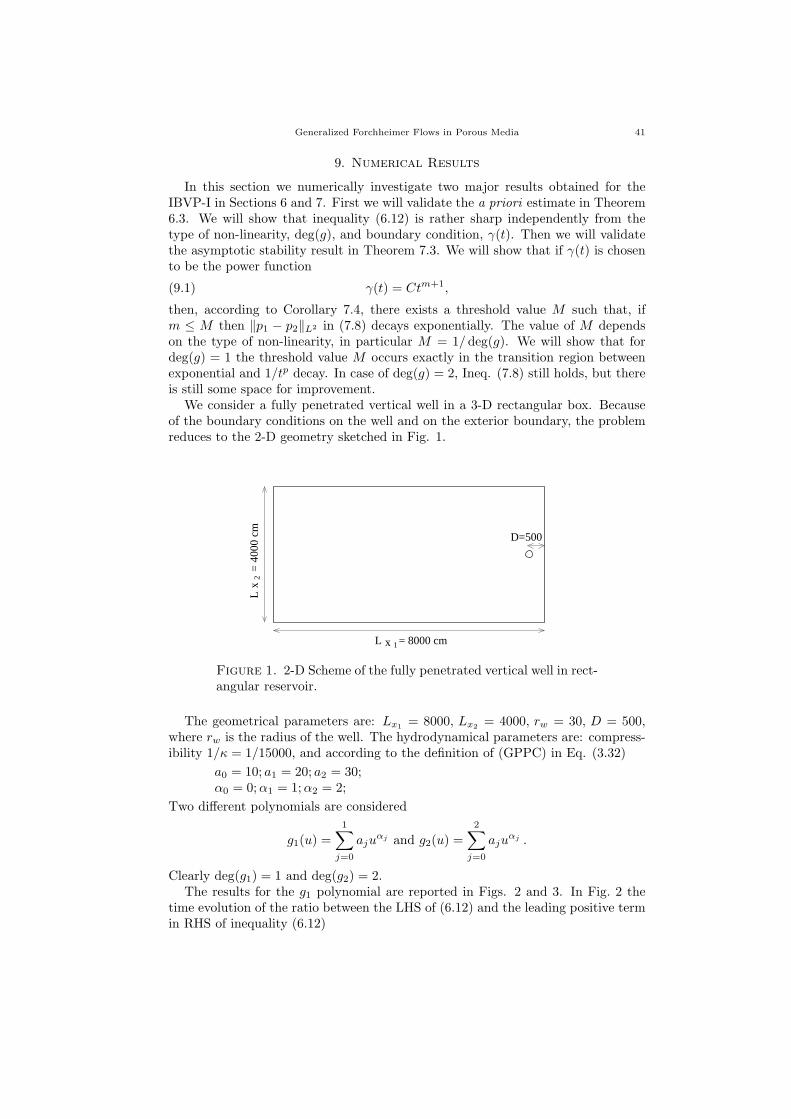
Generalized Forchheimer Flows in Porous Media 41
9. Numerical Results
In this section we numerically investigate two major results obtained for theIBVP-I in Sections 6 and 7. First we will validate the a priori estimate in Theorem6.3. We will show that inequality (6.12) is rather sharp independently from thetype of non-linearity, deg(g), and boundary condition, γ(t). Then we will validatethe asymptotic stability result in Theorem 7.3. We will show that if γ(t) is chosento be the power function
(9.1) γ(t) = Ctm+1,
then, according to Corollary 7.4, there exists a threshold value M such that, ifm ≤ M then ‖p1 − p2‖L2 in (7.8) decays exponentially. The value of M dependson the type of non-linearity, in particular M = 1/deg(g). We will show that fordeg(g) = 1 the threshold value M occurs exactly in the transition region betweenexponential and 1/tp decay. In case of deg(g) = 2, Ineq. (7.8) still holds, but thereis still some space for improvement.
We consider a fully penetrated vertical well in a 3-D rectangular box. Becauseof the boundary conditions on the well and on the exterior boundary, the problemreduces to the 2-D geometry sketched in Fig. 1.
2L
= 4
000
cmx
x 1L = 8000 cm
D=500
Figure 1. 2-D Scheme of the fully penetrated vertical well in rect-angular reservoir.
The geometrical parameters are: Lx1 = 8000, Lx2 = 4000, rw = 30, D = 500,where rw is the radius of the well. The hydrodynamical parameters are: compress-ibility 1/κ = 1/15000, and according to the definition of (GPPC) in Eq. (3.32)
a0 = 10; a1 = 20; a2 = 30;α0 = 0;α1 = 1;α2 = 2;
Two different polynomials are considered
g1(u) =1∑
j=0
ajuαj and g2(u) =
2∑
j=0
ajuαj .
Clearly deg(g1) = 1 and deg(g2) = 2.The results for the g1 polynomial are reported in Figs. 2 and 3. In Fig. 2 the
time evolution of the ratio between the LHS of (6.12) and the leading positive termin RHS of inequality (6.12)

42 E. Aulisa, L. Bloshanskaya, L. Hoang, A. Ibragimov
(9.2) R(t) =
∫UK (|∇p(x, t)|) |∇p(x, t)|2 dx
|U | ∫ t
0(γ′(τ))2 dτ
is given for different values of m in Eq. (9.1). From the top to the bottom on they-axis the values of m are equal to 0., 0.5, 0.6, 0.8, 1, 1.5, respectively. Clearly, foreach case the denominator in (9.2) diverges. The x − axis is in logarithmic scale.In the long time dynamics, only for m = 0 the ratio (9.2) converges to zero. This isjustified to the fact that in this case the PSS solution is reached and the numeratorconverges to some constant value, while the denominator diverges. On the otherhand for all the other values of m the ratio in (9.2) stabilizes to some value graterthan zero but less than one. This shows that numerator and denominator in (9.2)diverge with the same speed, or the same LHS and RHS of (6.12) diverge with thesame speed.
Figure 2. Time evolution of R(t) in Eq. (9.2), for g2 and differentvalues of m. From the top to the bottom on the y-axis m takesvalues 0., 0.5, 0.6, 0.8, 1, 1.5.
In Fig. 3 the time evolution of the norm ‖p1 − p2‖L2 is reported for the samevalues of m as before, while the order on the y-axis is reversed. Here p1(t, x) andp2(t, x) are two distinct solutions of the same IBVP-I with different initial pressuredistributions p1(0, x) and p2(0, x), respectively. Both the x-axis and the y-axis arein logarithmic scale. According to Corollary 7.4 exponential convergence is expectedfor m < 1. From the picture, it is clear that for m = 0., 0.5, 0.6, 0.8 all the curvesare concave down and ln ‖p1 − p2‖L2 → −∞ as ln t → −∞. This corresponds to‖p1−p2‖L2 ≤ C0e
−(tp), for some positive p. On the other hand for m = 1 the curve(the bold one) is a straight line and although it still diverges to −∞, it divergesmuch more slowly: ‖p1 − p2‖L2 ≤ C0t
−p, for some positive p. For m = 1.5 thecurve becomes concave up and it fails to diverge.
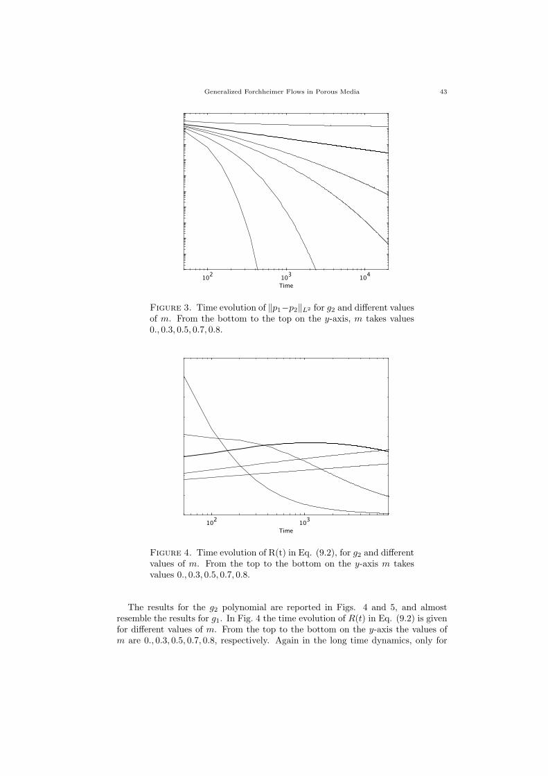
Generalized Forchheimer Flows in Porous Media 43
Figure 3. Time evolution of ‖p1−p2‖L2 for g2 and different valuesof m. From the bottom to the top on the y-axis, m takes values0., 0.3, 0.5, 0.7, 0.8.
Figure 4. Time evolution of R(t) in Eq. (9.2), for g2 and differentvalues of m. From the top to the bottom on the y-axis m takesvalues 0., 0.3, 0.5, 0.7, 0.8.
The results for the g2 polynomial are reported in Figs. 4 and 5, and almostresemble the results for g1. In Fig. 4 the time evolution of R(t) in Eq. (9.2) is givenfor different values of m. From the top to the bottom on the y-axis the values ofm are 0., 0.3, 0.5, 0.7, 0.8, respectively. Again in the long time dynamics, only for

44 E. Aulisa, L. Bloshanskaya, L. Hoang, A. Ibragimov
m = 0, R(t) converges to zero. For all the other values of m the ratio in (9.2)stabilizes to some value grater than zero but less than one. This shows that evenfor the g2 case the LHS and RHS of (6.12) diverge with the same speed.
In Fig. 5 the time evolution of ‖p1 − p2‖L2 is reported for the same values ofm. Here p1(t, x) and p2(t, x) are as before. According to Corollary 7.4 exponentialconvergence is expected form < 0.5. From the picture, it is clear that form = 0., 0.3all the curves are concave down. This corresponds to ‖p1 − p2‖L2 ≤ C0e
−(tp), forsome positive p. In this case even for m = 0.5, 0.7 the graph are still concavedown, and only for m = 0.8 a straight line is obtained. This shows that for g2the transition region occurs a little bit later that 0.5. This does not contradictCorollary 7.4, but only indicates that estimate (7.11) for g2 is less sharper thansame estimate for g1.
Figure 5. Time evolution of ‖p1−p2‖L2 for g2 and different valuesof m. From the bottom to the top on the y-axis, m takes values0., 0.5, 0.6, 0.8, 1, 1.5.
References
[1] M. A. Abodun, Mathematical Model for Darcy-Forchheimer Flow with application to WellPerformance Analysis, Master Thesis in Petroleum Engineering, Texas tech university, Lub-bock, June, 2007.
[2] L. Ai, K. Vafai, A coupling model for macromolecule transport in a stenosed arterial wall,International Journal of Heat and Mass Transfer 49 (2006) 1568–1591.
[3] E. Aulisa, A. I. Ibragimov, P. P. Valko, J. R. Walton, A new method for evaluation theproductivity index for non-linear flow, accepted SPE journal 108984.
[4] E. Aulisa, A. I. Ibragimov, P. P. Valko, J. R. Walton, Mathematical Frame-Work For Pro-ductivity Index of The Well for Fast Forchheimer (non-Darcy) Flow in Porous Media. Pro-ceedings of COMSOL Users Conference 2006, Boston (2006).
[5] E. Aulisa, A. Cakmak, A. Ibragimov, A. Solynin, Variational Principle and Steady State In-variants for Non-Linear Hydrodynamic Interactions in Porous Media, DCDIS A Supplement,Advances in Dynamical Systems, Vol. 14(S2) 148–155, 2007.
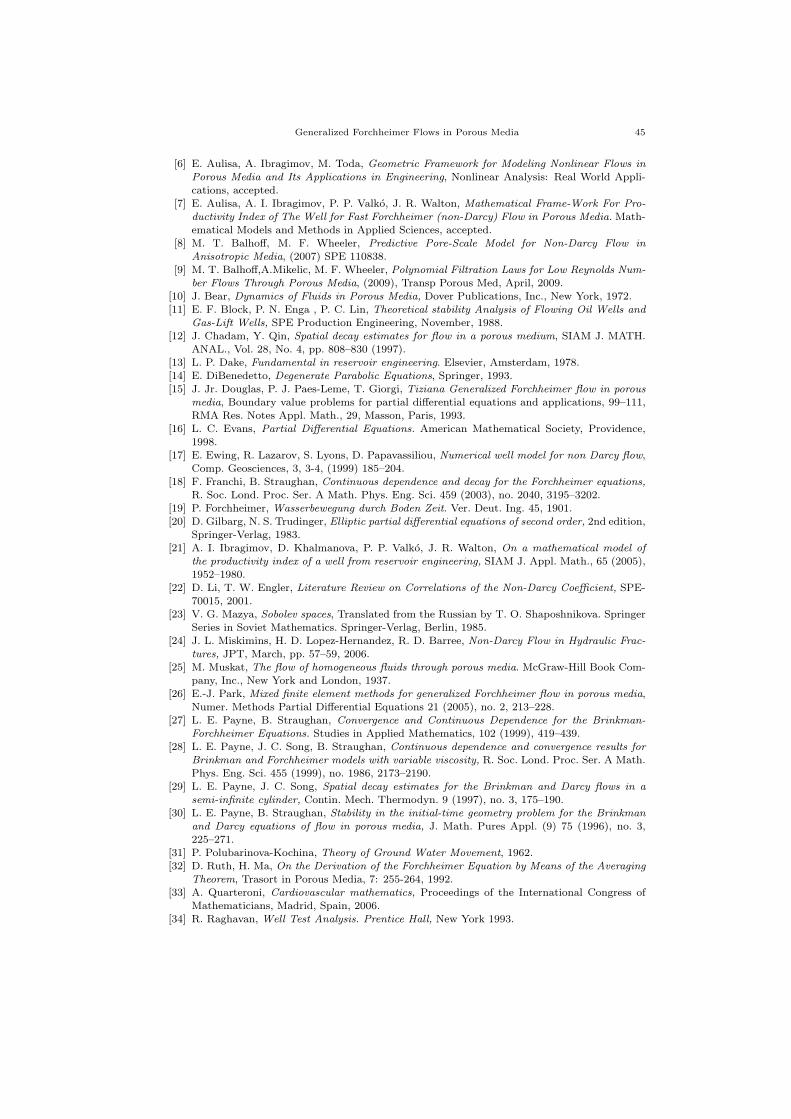
Generalized Forchheimer Flows in Porous Media 45
[6] E. Aulisa, A. Ibragimov, M. Toda, Geometric Framework for Modeling Nonlinear Flows inPorous Media and Its Applications in Engineering, Nonlinear Analysis: Real World Appli-cations, accepted.
[7] E. Aulisa, A. I. Ibragimov, P. P. Valko, J. R. Walton, Mathematical Frame-Work For Pro-ductivity Index of The Well for Fast Forchheimer (non-Darcy) Flow in Porous Media. Math-ematical Models and Methods in Applied Sciences, accepted.
[8] M. T. Balhoff, M. F. Wheeler, Predictive Pore-Scale Model for Non-Darcy Flow inAnisotropic Media, (2007) SPE 110838.
[9] M. T. Balhoff,A.Mikelic, M. F. Wheeler, Polynomial Filtration Laws for Low Reynolds Num-ber Flows Through Porous Media, (2009), Transp Porous Med, April, 2009.
[10] J. Bear, Dynamics of Fluids in Porous Media, Dover Publications, Inc., New York, 1972.[11] E. F. Block, P. N. Enga , P. C. Lin, Theoretical stability Analysis of Flowing Oil Wells and
Gas-Lift Wells, SPE Production Engineering, November, 1988.[12] J. Chadam, Y. Qin, Spatial decay estimates for flow in a porous medium, SIAM J. MATH.
ANAL., Vol. 28, No. 4, pp. 808–830 (1997).[13] L. P. Dake, Fundamental in reservoir engineering. Elsevier, Amsterdam, 1978.[14] E. DiBenedetto, Degenerate Parabolic Equations, Springer, 1993.[15] J. Jr. Douglas, P. J. Paes-Leme, T. Giorgi, Tiziana Generalized Forchheimer flow in porous
media, Boundary value problems for partial differential equations and applications, 99–111,RMA Res. Notes Appl. Math., 29, Masson, Paris, 1993.
[16] L. C. Evans, Partial Differential Equations. American Mathematical Society, Providence,1998.
[17] E. Ewing, R. Lazarov, S. Lyons, D. Papavassiliou, Numerical well model for non Darcy flow,Comp. Geosciences, 3, 3-4, (1999) 185–204.
[18] F. Franchi, B. Straughan, Continuous dependence and decay for the Forchheimer equations,R. Soc. Lond. Proc. Ser. A Math. Phys. Eng. Sci. 459 (2003), no. 2040, 3195–3202.
[19] P. Forchheimer, Wasserbewegung durch Boden Zeit. Ver. Deut. Ing. 45, 1901.[20] D. Gilbarg, N. S. Trudinger, Elliptic partial differential equations of second order, 2nd edition,
Springer-Verlag, 1983.[21] A. I. Ibragimov, D. Khalmanova, P. P. Valko, J. R. Walton, On a mathematical model of
the productivity index of a well from reservoir engineering, SIAM J. Appl. Math., 65 (2005),1952–1980.
[22] D. Li, T. W. Engler, Literature Review on Correlations of the Non-Darcy Coefficient, SPE-70015, 2001.
[23] V. G. Mazya, Sobolev spaces, Translated from the Russian by T. O. Shaposhnikova. SpringerSeries in Soviet Mathematics. Springer-Verlag, Berlin, 1985.
[24] J. L. Miskimins, H. D. Lopez-Hernandez, R. D. Barree, Non-Darcy Flow in Hydraulic Frac-tures, JPT, March, pp. 57–59, 2006.
[25] M. Muskat, The flow of homogeneous fluids through porous media. McGraw-Hill Book Com-pany, Inc., New York and London, 1937.
[26] E.-J. Park, Mixed finite element methods for generalized Forchheimer flow in porous media,Numer. Methods Partial Differential Equations 21 (2005), no. 2, 213–228.
[27] L. E. Payne, B. Straughan, Convergence and Continuous Dependence for the Brinkman-Forchheimer Equations. Studies in Applied Mathematics, 102 (1999), 419–439.
[28] L. E. Payne, J. C. Song, B. Straughan, Continuous dependence and convergence results forBrinkman and Forchheimer models with variable viscosity, R. Soc. Lond. Proc. Ser. A Math.Phys. Eng. Sci. 455 (1999), no. 1986, 2173–2190.
[29] L. E. Payne, J. C. Song, Spatial decay estimates for the Brinkman and Darcy flows in asemi-infinite cylinder, Contin. Mech. Thermodyn. 9 (1997), no. 3, 175–190.
[30] L. E. Payne, B. Straughan, Stability in the initial-time geometry problem for the Brinkmanand Darcy equations of flow in porous media, J. Math. Pures Appl. (9) 75 (1996), no. 3,225–271.
[31] P. Polubarinova-Kochina, Theory of Ground Water Movement, 1962.[32] D. Ruth, H. Ma, On the Derivation of the Forchheimer Equation by Means of the Averaging
Theorem, Trasort in Porous Media, 7: 255-264, 1992.[33] A. Quarteroni, Cardiovascular mathematics, Proceedings of the International Congress of
Mathematicians, Madrid, Spain, 2006.[34] R. Raghavan, Well Test Analysis. Prentice Hall, New York 1993.
46 E. Aulisa, L. Bloshanskaya, L. Hoang, A. Ibragimov
[35] K. R. Rajagopal, On a hierarchy of approximate models for flows of incompressible fluidsthrough porous solids, Mathematical Models and Methods in Applied Sciences, Vol. 17, No.2 (2007) 215–252.
[36] K. R. Rajagopal, L. Tao, Mechanics of mixtures, World scientific, (1995).[37] E. Sanchez-Palencia, Non-Homogeneous Media and Vibration Theory, Lecture Notes in
Physics, Springer-Verlag, 1980.[38] C. A. P. Tavera, H. Kazemi, E. Ozkan, Combine effect of Non-Darcy Flow and Formation
Damage on Gas Well Performance of Dual-Porosity and Dual Permeability Reservoirs, SPE-90623, 2004.
[39] B. Wang, S. Lin, Existence of global attractors for the three-dimensional Brinkman-Forchheimer equation, Math. Methods Appl. Sci. 31 (2008), no. 12, 1479–1495.
[40] M. F. Wheeler, M. Peszynska, Computational engineering and science methodologies formodeling and simulation of subsurface applications, Adv. in Water Resources, 25 (2002)1147–1173.
[41] S. Whitaker, The Forchheimer Equation: A Theoretical Development, Transport in PorousMedia 25: 27–61, 1996.
Department of Mathematics and Statistics, Texas Tech University, Box 41042, Lub-bock, TX 79409–1042, U. S. A.
E-mail address: [email protected]
E-mail address: [email protected]
E-mail address: [email protected]
E-mail address: [email protected]