Analysis of a rate-based feedback control strategy for long haul data transport

Performance Evaluation 16 (1992) 67-84 North-Holland

67

Analysis of a rate-based feedback control strategy for long haul data transport

Kerry W. Fendick, Manoe l A. Rodr igues and Alan Weiss A T&T Bell Laboratories, Murray Hill, NJ 07974, USA

Abstract

Fendick, K.W., M.A. Rodrigues and A. Weiss, Analysis of a rate-based feedback control strategy for long haul data transport, Performance Evaluation 16 (1992) 67-84.

Digital communication has become fast enough so that the speed of light has become a bottleneck. For example, the round trip transcontinental [USA] delay through a fiber link is approximately 0.04 s; at 150 Megabit/s, a source needs to transmit approximately 8,000,000 bits during one round trip time to utilize the bandwidth fully. As the service rates of queues get large, the time scales of congestion in those queues decrease relative to the round trip time, making the dual goals of keeping buffers small and utilization~ high even more difficult to achieve. In this paper we analyze a class of delayed feedback schemes that achieve these goals despite propagation delays and regardless of network rates. We analyze the delayed feedback schemes as a system of delay-differential equations, in which we model the queue-length process and the rate at which a source transmits data as fluids. We assume that a stream of acknowledgements carries information about the state of a bottleneck queue back to the source, which adapts its transmission rate according to any monotone function of that state. We show stability for this class of schemes, in that their rate of transmission and queue length rapidly converge to a small neighborhood of the designed operating point. We identify the appropriate scaling of the moael's parameters, as a function of network speed, for the system to perform optimally: with a deterministic service rate of /z at the bottleneck queue, the steady state utilization of the queue is 100-O(/z-1/2)% and steady state delay is O(tt-1/2). We also describe the transient of behavior of the system as another source suddenly starts competing for the bandwidth resources at the bottleneck queue. This work directly applies to the adaptive control of Frame Relay and ATM networks, both of which provide feedback to users on congestion.

Keywords: data networks; adaptive flow control; delay-differential equations.

1. Introduction

Packet switching represents an attractive data networking technology for its efficiency and flexi- bility, resulting from the dynamic sharing of network resources among users. Although the sharing of resources results in significant advantages it also results in disadvantages due to the inher- ent interference among users. This interference causes undesirable effects, such as packet loss and high delays, which are exacerbated under overload conditions. Thus, a large body of work spread over several areas (e.g., flow control [4], congestion control [2], window control [12], rate

Correspondence to: Dr. M.A. Rodrigues, AT&T Bell Labs, Room 1F-412, 101 Crawfords Corner Road, P.O. Box 3030, Holmdel, NJ 07733-3030, USA.

control [3], etc.) has sought the common objective of finding the right balance between efficiency and "fairness" through proper monitoring and controlling the offered load.

With the ever increasing speeds of data transmission, the control of the traffic has become an even more difficult problem. Digital communication has become fast enough so that propagation delay is now a major factor. For example, a round trip transcontinental [USA] delay through a fiber link is approximately 0.04 s; to obtain full utilization of a 150 Megabit/s channel, it would be necessary to maintain an amount of outstanding data of approximately 8,000,000 bits (or 1 Mbyte, or 1000 1K packets) during one round trip time. Providing high efficiency while keeping delay and packet loss within acceptable levels is not feasible in this environment by just using static control;

0166-5316/92/$05.00 © 1992 - Elsevier Science Publishers B.V. All rights reserved

68 K.W. Fendick et al. / Rate-based feedback control strategy

i.e., we need efficient dynamic schemes that can adaptively conform to the environment.

Several dynamic schemes for congestion control/avoidance have been proposed. Jain [10] proposed the use of implicit congestion signals provided by timeouts to bring window sizes down immediately to a predetermined minimum value; under normal operation he prescribed a linear increase of the window size up to a predetermined maximum level. Jacobson [9] suggested the use of an adaptive scheme that increases the window size linearly and decreases it exponen. tially in case of congestion. Congestion is de- tected through a timeout control mechanism that takes into account the variability of the round-trip time, later to be incorporated in the Berkeley UNIX TCP. Ramakrishnan and Jain [17] proposed an adaptive scheme that also increases the window size linearly and decreases it exponen- tially. Their scheme is based on an explicit single bit per packet feedback signal that relays information about busy periods at the queue to the users of the network. Later, Bolot and Shankar [1] modeled an adaptive scheme, similar to the one proposed by Ramakrishnan and Jain, as a set of coupled differential equations and obtain analytical closed-form solutions for the transient and steady-state behavior of this model. Mukherjee and Strikwerda [16] were able to capture through analysis some of the effects of delayed feedback on the performance of adaptive congestion control schemes based on linear-increase-exponen- tial-decrease algorithms. Mitra ['i2] proposed a dynamic adaptive algorithm, based on estimating queue size through measured packet acknowl-

edgement times, which attempts to prevent rather than react to congestion, targeting convergence of window size and queue size towards an optimal operating point. Making further assumptions about the nature of the network can lead to different controls. That is the case in the papers by Keshav [11] and Hahne et al. [5], where all nodes are assumed to implement a processor sharing service discipline. Keshav proposed a dynamic rate control algorithm based on estimating the available bandwidth at the bottleneck link of a connection, and Hahne et al. [5] proposed a centralized dynamic window allocation scheme. Both take advantage of the predictability of service rates under the processor sharing discipline.

These schemes may prove to be effective in preventing or reacting to congestion. However, in all these schemes (except those by Keshav [11] and Hahne et al. [5], which assume perfect knowl- edge of available service rates), both the window size and queue size oscillate. The oscillatory behavior suggests that there may be some fundamental instability that could be understood and captured analytically. Furthermore, as speed increases, the time scales of congestion in a queue decrease relative to the round trip time. Thus, the dual goals of keeping buffers small and uti- lizations high is difficult to achieve even with dynamic schemes; any end-to-end control system with feedback can react to congestion only after transmitting, and possibly losing, large volumes of data. Therefore, it is important ~a t large prolaa- gation delays and high speeds be taken into con- sideration when analyzing control of systems for high speed, long haul data transport. Note that

Kerry W. Fendick graduated from Colgate University in 1982 with a B.A. in Mathematics and Economics and from Clemson University in 1984 with a M.S. in Mathematics. Since 1984 he has worked at AT&T Bell Laboratories as a member of the Data Network Analysis Department. He is interested in the measurement and control of queueing systems, particularly as applied to packet data networks.

Manoei A. Rodrigues received the B.S.E.E. degree from the Universidade Federal do Rio de Janeiro, Rio de Janeiro, Brazil in 1982, and the M.S.E.E., C. Phil., and Ph.D. degree in electrical engineering (communication theory and systems) from the University of California at San Diego, La Jolla, CA, in 1985, 1986 and 1987, respectively. He was with Moddata S.A. Engenharia de Telecomunicacoes e Informatica, Brazil, from 1980 to 1984. He has been a Member of Technical Staff at AT&T Bell Laboratories since 1987. His work involves performance analysis of data networks and his research interests are in stochastic modeling of queueing systems, multiaccess networks, communication protocols, routing protocols and high-speed networking architectures.

Alan Weiss graduated in 1976 from Case Western Reserve University with degrees in Physics and Mathematics, and in 1981 from the Courant Institute of Mathematical Sciences in Mathematics. Since then he has been at AT&T Bell Labs, concentrating on the applications of the theory of large deviations to communication and computer systems.

K.W. Fendick et ai. / Rate-based feedback control strate~;y 69

these parameters are available to the designers of such systems. Given that a good feedback control system should work well for a wide range of speeds, the question of how parameters should scale with speed still remains unanswered.

In this paper we address the questions identi- fied in the previous paragraph: what are the stability properties of a large class of dynamic rate/windowing control algorithms with delayed feedback, and how should parameters scale with speed. Although on one hand we consider a very general set of controls, on the other hand we restrict ourselves to the simplest possible network case: that of a single session and a single bottleneck node. The reason for considering such a simple reference connection is that there are fundamental questions about the limitations of dynamic adaptive systems with delayed feedback that we would like to capture which could get diffused in a more complex environment. We also investigate the transient behavior of such systems upon sudden changes in the available bandwidth.

The paper is organized as follows: In Section 2 we describe our primary model, which is based on a set of delay differential equations. We then show how to derive the specific equations that approximate the adaptive windowing scheme of Mitra and Seery [13] as a continuous deterministic fluid model. We chose their scheme because it is designed to have nearly optimal throughput and delay, and uses minimal signaling for feedback. Note, however, that we model a rate controlled system while their system is window controlled. In Section 3 we describe our results in terms of five theorems. In Section 4 we interpret the theorems and discuss our four major results: stability, scaling, transient behavior and generality. We develop an analysis technique and we apply it to the particular set of equations that describes the scheme proposed by Mitra and Seery. We show that the system is stable in the sense that the rate of transmission and the queue size are rapidly confined to a small neighborhood of the designed operating point. We also show that the design operating point is an unstable equilibrium point; the system must oscillate around the equilibrium point. We identify the correct scaling for parameters associated with a model, and we show that the size of the stability region can be designed through the choice of parameter values. We calculate the transient be-

havior of our model for a given abrapt change of the available resources. Finally, we show that this stability is unchanged over a wide class of perturbations of the model, thus encompassing a large class of control functions and feedbacks. In Sec- tion 5 we provide some discussion on the equivalence of rate and window control. In Section 6 we state our conclusions. The proofs of the theorems are presented in the appendices.

2. The model

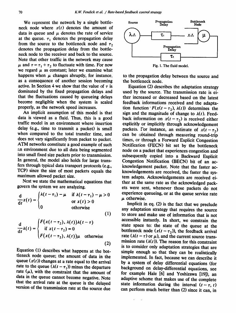
We consider the model of a virtual circuit depicted in Fig. 1. It constitutes a single session between a source and a destination through a network. We assume that the source transmits at a rate A(t) during the life of a session; its objective is to choose the value of A(t) at all time such that the source gets as much throughput from the network as possible without causing excessive congestion. This performance objective can be stated in terms of maximizing power [12].

We assume that the source has an infinite amount of data to send, so that a session goes on forever. This assumption is important since it isolates the issue of adaptive control mechanisms effectiveness from other considerations. Further- more, we can derive the corresponding results for large but finite amounts of data based on the transient and the long run behavior of the system for a source with infinite amounts of data. How- ever, the model is still restricted to large file transfers and the like, not all types of connec- tions. Large transfers are important for several reasons: they represent a large fraction of traffic on a network, and the congestion they induce has to be handled well since they will have the most noticeable effects on network performance. Al- though we do not wish to overlook the impor- tance of other types of traffic that do not match our model, like interactive traffic, their effect on network performance is quite different from that of large transfers. Their primarily effect is that of causing additional noise to the adaptation of file transfer sessions. The adaptive aspects of control schemes will neither hurt nor help performance when transmitting short messages. Thus, we sim- ply defer their study to a future paper and we focus this paper on the fundamental question of adaptation for large transfers.


We represent the network by a single bottleneck node where x(t) denotes the amount of data in queue and/z denotes the rate of service at the queue. ¢t denotes the propagation delay from the source to the bottleneck node and ¢2 denotes the propagation delay from the bottleneck node to the receiver and back to the source. Note that other traffic in the network may cause /z and ¢ = c m + re to fluctuate with time. For now we regard/z as constant; later we examine what happens when /~ changes abruptly, for instance, as a consequence of another session becoming active. In Section 4 we show that the value of ¢ is dominated by the fixed propagation delays and that the fluctuations caused by queueing delays become negligible when the system is scaled properly, as the network speed increases.

An implicit assumption of this model is that data is viewed as a fluid. Thus, this is a good traffic model in an environment where insertion delay (e.g., time to transmit a packet) is small when compared to the total transfer time, and does not vary significantly from packet to packet. ATM networks constitute a good example of such ran environment due to all data being segmented into small fixed size packets prior to transmission. In general, the model also holds for large transfers through typical data transport protocols (e.g., TCP) since the size of most packets equals the maximum allowed packet size.

Next we state the mathematical equations that govern the system we are analyzing.

d (i(t-1"l)-/z -d~x( t ) =

if A ( t - ¢!) - I t > 0

or x(t) > 0 otherwise

(1)

d IF(x ( t -¢2) , a ( t ) )h ( t - ¢)

~ ' h ( t ) = ~ if x ( t - ¢ 2 ) = 0

l ,F(x( t -r2) , ,~(t))/z otherwise

(2)

Equation (1) describes what happens at the bottleneck node queue; the amount of data in the queue (x(t)) changes at a rate equal to the arrival rate to the queue (a(t - ¢~)) minus the departure rate (/z), with the constraint that the amount of data in the queue cannot become negative. Note that the arrival rate at the queue is the delayed version of the transmission rate at the source due

Source Propagation Delay

] "C, l X(t)

Propagation , Delay

Fig. 1. The fluid model.

Bottleneck Node

to the propagation delay between the source and the bottleneck node.

Equation (2) describes the adaptation strategy used by the source. The transmission rate is either increased or decreased based on the latest feedback informations received and the adaptation function'F(x(t- ¢2), A(t)) determines the sign and the magnitude of change to A(t). Feed- back information on x ( t - ¢2) is received either explicitly or implicitly through acknowledgement packets. For instance, an estimate of x ( t - z2) can be obtained through measuring round-trip times, or through a Forward Explicit Congestion Notification (FECN) bit set by the bottleneck node on a packet that experiences congestion and subsequently copied into a Backward Explicit Congestion Notification (BECN) bit of an acknowledgement packet. Note that the faster acknowledgements are received, the faster the system adapts. Acknowledgements are received either at the same rate as the acknowledged packets were sent, whenever those packets do not experience queueing, or at the queue service rate /z otherwise.

Implicit in eq. (2) is the fact that we preclude any adaptation strategy that requires the source to store and make use of information that is not accessible instantly. In short, we constrain the state space to: the state of the queue at the bottleneck node ( x ( t - ¢2)), the feedback arrival rate (A(t - ¢) or/~), and the current source transmission rate (A(t)). The reason for this constraint is to consider only adaptation strategies that are simple enough so that they can be realistically implemented. In fact, because we can describe it by a system of delay differential equations (for background on delay-differential equations, see for example Hale [6] and Yoshizawa [19]), an adaptive scheme that makes use of the complete state information during the interval ( t - r, t) can perform much better than (2) since it can, in

K W. Fendick et aL / Rate-based feedback control strategy 71

principle, predict the behavior of the system. On the other hand, since this is a continuous time system, an infinite amount of memory space would be required to store information about the value of any single variable during any interval. More importantly, such a system would not adapt as well as ours to changing traffic conditions. Al- though there is a large number of adaptation strategies that our model does not cover, we believe that it covers a large class of system that are of interest.

We describe next how Mitra and Seery's adaptive scheme can be modeled in terms of eqs. (1) and (2). There are two steps involved in this transformation, the first one being that of transforming a discrete system into a continuous fluid system while the other is writing their adaptation scheme in terms of eq. (2). They proposed the following: if K,, is the size of the window (i.e., the amount of outstanding unacknowledged data) at the nth acknowledgement, and if R,, is the round-trip delay of the nth packet, then

K,,+, =K, , -A ( (R , , - r )C-~ . - b ) (3)

where b = 1 and A is chosen (by simulation study) to make the scheme perform well.

Let us see how Mitra and Seery's scheme fits into our framework. The equation for £(t) follows directly from transforming the source from a discrete source into a continuous fluid source. Since x(t) is completely defined once A(s), for s ~ (0, t - I-1), is defined, the fluid version of A(s) determine x(t). We can approximate the rate of transmission at the source by the throughput of the windowing system [18]:

gn t,) = '

w h e r e t n is the time when the source receives the nth acknowledgement. Since propagation delays dominate the round-trip delay for high-speed networks, to first order we can ignore the queueing delay when calculating the window throughput. Thus, the equivalent fluid rate at the source becomes:

gn A(t,) = . (4)

T

Nonetheless, the queueing delay can be obtained through round-trip delay measurements:

X(t --'r2) . ( 5 ) /.L

In Mitra and Seery's scheme, the source adapts according to eq. (3) every time an acknowledgement is received. Therefore, the rate of acknowledgements will also dictate the rate of adaptation. Note that when packets find the queue is empty, acknowledgements return at the same rate as the packets that are being acknowledged were transmitted. On the other hand, when packets find the queue non-empty, acknowledgements return at the rate in which packets are served at the bottleneck queue. Thus the time between adapta- tions can be stated as:

A t = A(t--"rl--~'2) 1 /z

if x ( t - T 2 ) = 0,

otherwise.

(6)

Thus, we can approximate the adaptation strategy by:

d AA ( K,,+ I - K,) ~-~A(t) = At = ¢ A~ (7)

x(t - "/'2) ) = a -~ ¢rff (( t ) - 1 / A t . (8 )

The approximation above would be exact if the original traffic we are modelling were a fluid. After substituting eq. (6) into eq. (8) and then into eq. (2),

(x(t- , , ) ) a t ro t ) - 1 A(

/z

d if X( t -- 'rE) -- 0 ,

-d - tA ( t )=(x ( t - ' r2 ) ) a C r Y ) - 1 .

/z

otherwise.

t - ~t - T 2 )

(9)


For sake of simplicity we initially assume that A =/z + O ( ~ ) , so that

d I ~-TA(t) =

x ( t - ¢ 2 ) - 1 A ( t - - T 1

f ; if x ( t - z2) = 0,

X(t --'r2) ) - 1 ~

otherwise.

-- T2)

(10)

the initial conditions. For the optimal scaling a = 1 / vr-~, there exist constants m,n > 0 independent of the initial conditions such that Y(Iz)= m vr~ and A+(tz) = A - ( # ) =n¢-~.

Theorem 3. For the optimal scaling a = 1 / Vf-~, no neighborhood of the point (x = B, A = Ix) can ultimately bound the solution (x(t), A(t)) as t-~oo without including the boundary at x = O. Solution paths consist of an infinite sequence of excursions away from x = 0 and back again.

That is, Mitra and Seery's scheme has a linear function F(x/V/-~). Later we will show that we should have a ~ 1 / ~ and that A converges to a region bounded by /z ± O(~'~), which suggests that the two systems (9) and (10) should indeed behave similarly. We then prove that our results on the convergence of (10) extend to cover (9) as well as a large class of perturbations of (10).

3. Results

Theorem 4. For an abrupt change of order 0 (# ) to the service rate at the bottleneck node, there will be a change of order O(Iz ) to the buffer occupancy before the system adapts again.

Theorem 5. For the optimal scaling a = 1 / V ~ , the conclusions of Theorem 2 hold under any modi- fications of its assumptions that preserve the total transient structure, and change dA / d t by order

~ for (A, x) within the box (0, m~r~) x (1~ - n

We now state our results on the delay-differential equations. The proofs are given in the appendices. For Theorems 1-3, we introduce f (x) defined by (x) F( x) f a f - - ~ - b , ( i l )

where b = B / ~ and f ( - b) are O(1) with f ( x ) monotone non-increasing and f (0 )= 0. This rep- resentation of F is less general than (2) but more general than (10). In Theorem 5 we extend our results to cover the more general F in (2). Later we show that we optimally should have a ~

Theorem 1. The point (x(t)=B, A(t)=#) is an unstable equilibrium point.

Theorem 2. For general a and each f(x) monotone decreasing with - b <~ x <~ oo, there are bounded fimctions Y(lz ), A - (Iz ), A + (#) > O, independent of initial conditions, such that

O ~ x ( t ) < Y(Iz)

# - A - ( # ) ~<a(t) </z +A+(/z)

for all t large enough, t > T where T depends on

4. Interpretation of the Theorems

The theorems from the previous section sup- port four basic results: stability, scaling, transient and generalizations. Theorems 1, 2 and 3 give insight on both the stability behavior of the system as well as on the proper scaling of parameters. The obtained results confirm some general behavior that has been observed in many adaptive rate/window control mechanisms: the system appears stable (Theorem 2), but not when you look too closely (Theorems 1 and 3). That is, a high-speed system with delays will jitter, but only a bounded amount. Theorem 3 shows in a Lia- punov sense that the boundary at x(t) = 0, which corresponds to the queue at the bottleneck node being empty, is responsible for the stability of the system. The proper scaling to the system also is derived in Theorem 2, where a particular change of variables results in a system of equations that become independent of the speed at the bottleneck in the limit as the speed gets large. It shows that the jitter can be made effectively small. The- orem 4 describes what happens to the system during transients. It shows that whenever there is

K W. Fendick et al. / Rate-based feedback control strategy 73

an abrupt change in bandwidth, it is inevitable to have queue occupancies of order O (/x), suggest- ing that some sort of slow start mechanism is essential if small buffers are desirable. Theorem 5 shows that our results hold in greater generality for a large class of adaptation schemes and feedback information. Next we discuss each of these results in more details.

It is clear that the points (B,/~) and (0, 0) are equilibrium points for our system of delay-differential equations. A point is defined as an equilibrium point for a system of delay-differential equations if the solutions remain forever at that point after having been there for at least an amount of time corresponding to the memory of the system, which in this case equals ¢. It would be desirable that the point (B,/z) were a stable equilibrium point. That would imply that our system is well behaved like many other control systems. However, that is not true and we show in Appendix A that the equilibrium point (B, ~) is in fact unstable for a perturbed version of the system, where we treat z as a small parameter and we linearize the system of equations around the equilibrium point. Although this particular approach is not a rigorous proof, it suggests that the stability of the system is not a simple one. A rigorous proof of the stability of the system and its behavior around the equilibrium point is given in Appendices B and C.

The standard theory of delay-differential equations [6] does not treat the class of systems described by (1) and (2). In Appendix B we develop the necessary analytical tools and we show that the solutions to the system (1) and (2) are uniformly ultimately bounded for a large class of initial conditions. Thus, for all (well behaved) initial conditions, the solution path must enter a neighborhood of the equilibrium point (B,/z) and can never leave. Note that for a system of delay-differential equations, the solution path is no! gefined by a single point as initial condition but by a function defined over a time interval of length ~'. A more detailed discussion of well behaved initial conditions can be found in ,~ppendix B. '.the stability behavior of the system is depicted in Fig. 2. We show a family of trajectory paths over the (,L x) plane. In Appendix B we also derive tight bounds for the region R in terms of the adaptation strategy, the propagation delays and the bandwidth at the bottleneck node.

The behavior of the system inside region R is described in Appendix C. There we prove that a Lyapunov functions strictly increases over any cycle of the solution path around the equilibrium point that does not hit the boundary at x = 0. Note that while the stability results on Theorem 2 hold for any choice of parameters, the behavior inside region R described in a Lyapunov sense was only derived for when the optimal scaling a=l/l~.

The stability results suggest that the system is stable but it is prone to jitter. How much does the jitter affect performance? We are able to show that the proper scaling to the system corresponds to the change of variables given by equation (B.1). Stating it more explicitly we recommend that

- b ,

where b and f ( - b) and O(1). With this scaling, Theorem 3 implies that some

loss of throughput is inevitable in the long run, i.e., that the greatest lower bound on t-~f~a(t) as t --, 0o is strictly less than/z. On the positive side, we see that steady-state throughput is at least /~-VM~rqV~; that is, throughput is ( 1 0 0 - O(1 / l f~ ) )% of its theoretical maximum. Simi- larly, steady-state delay is ~- + (x(t))/it ~ ¢ + [(b + UMAX)lf~]//z = 1" + O(1 /V~) , which is close to the theoretical minimum ¢. Thus our scheme has achieved a level of performance that cannot be excelled in these respects. The definitions of vMm ~ and /'/MAX can be found in Appendix B. Another important consequence of using the proper scaling is that randomness caused by queueing delays in the network, are O(1/V/-~-). This is consistent with the assumption that propagation delays dominate the feedback delay ~" at high speeds.

It is intuitive that the propagation delay con- tributes to the increase in magnitude of the jitter in the system. We quantify that effect in Theorem 2 which shows that the bound on the jitter is approximately linear in ~" when ~" or f(-b) are large. The consequence of a linear increase in jitter is a linear increase in delay and in buffer requirements, which is reasonable.

With a bit more calculation we shall see that the transient behavior of our scheme is within a constant factor of optimal, and that any other


scaling would be worse. To this end we consider the scaled system given by equation (B. 1). So long as u(t - ~'2) > - b .

ti = v ( t - z l )

b = f ( u ( t - % ) )

still represents the exact same system. Since The- orem 2 states that v ( t - 1- l -~ '2 )= O(1), asymptotically

d d tU( t ) = v ( t - r l )

d - - v ( t ) = f (u ( t -~ '2 ) ) dt

approximates the behavior of the system also for u ( t - %,)= - b . That is, we have asymptotically (approximately)

ii = f ( u ( t - ~ ' ) ) ,

where r = r t + r 2, implying that the scaled system is nearly independent of tz; this means that the scaling is good. It also means that it is easy to estimate the transient response of the system, since it is nearly independent of/z.

N~w let us examine the effect of improper scaling of the timing parameters. The parameters a and b represent the amplification and center- ing of the scheme.

In order to have small buffers we would like to have b = 0. Indeed, this has no detrimental affect on the fluid model we have proposed. However, setting b too small makes the validity of the deterministic fluid model questionable as an approximation for a system with randomness. Mitra's study [12] shows that fluctuations in the buffer of order f ~ arc to be expected in a non-adaptive optimal wi~,.dow-based scheme. If we had our fluid model with b smaller than this, the criticism of inappropriate modeling is justL fled. However, larger b makes for longer delays without an appreciable gain in throughput, and the instability of the operating point appears more pronounced because the size of the bounding box is proportional to b. However, the more nearly deterministic a system is, the smaller b can be chosen without violating modeling assumptions. Similarly, the size of the bounding box would seem to shrink with a; hence, why not choose a very small value? The answer is that the transient behavior then becomes worse.

Consider what transpires if /.L is suddenly changed to /~/2, once (x(t), A(t)) have entered the bounding box. Theorem 4 addresses this question in more details. We have A(t)---/z for tE[0 , ~'], so

d /x ~ ' X ( t ) = ~-;

i.e. x(t) = (~ /2 ) t for t ~ (0, ~'). After time r, though, the system will adapt. If f ( x ) = x for large x, we see that the time required for A(t) to drop below/z/2 is O(1), and hence the maximum value of x(t) is O(/x), i.e. the buffer stays within a constant multiple of the best that any adaptive scheme subject to delay could achieve. With non- linear f (x ) the adaptation can be made even more quickly, but the maximum value of x(t) can never be less than ( / z / 2 ) r = O(/z), which is the claim of Theorem 4. Thus, it is not clear if cleverness in the design of f (x) is warranted.

Our scaling shows that a simulation (or othex) pilot study can be performed at one value of t~, then the system can be scaled up to a higher value by using the same values of a and b and scaling the controls according to F,(x). Also, an operating network can be sped up without delete- rious side effects by using our prescription.

Theorem 5 shows that our results hold for a wide variety of adaptation schemes. For example, Keshav [ 11] has proposed a scheme for estimating t~ directly. Without going into details, suppose that we have an estimate /2(t) that is a noisy estimate of tz(t). We can modify our adaptation scheme as follows:

-fiT X( t ) =

d

A ( t - r ) - ; , > 0

or x ( t ) > 0 otherwise

~-~A(t) - F (x ( t - ~'2))A( t - ~'2)

+ G~(~.( t - "1"2) - / ~ , ( t - 7"2) )~.( t - ' r 2 ) .

Here G(x)should have G(0)= 0, G monotone decreasing. Can such a scheme improve the stability of the estimate (x(t), ,~(t))? Can it make things worse? The short answer is: it depends on the quality of the approximation /2(t). Suppose that 12(t) - /~ = O ( ~ ) or smaller.

Proposition 1. I(x(t), A(t ) ) - (b , /~) l =O(I /2( t ) - ~ ] ) as t -,oo.

K IV. Fendick et al. / Rate-based feedback control strategy 75

That is, if / 2 ( t ) - - ~ ~ 0 as t ~ oo then (x, A)(t) (b, Iz). I f /2( t ) - / x = O(VI'~ ) then the stability

of the system is largely unaffected by the inclu- sion of the estimate. This implies to us that, unless the estimate /2 is very accurate, there is little advantage in using it. Note that in case the bottleneck node uses a processor sharing discipline, the estimate of tz can be very accurate for a slowly changing system. The proof of the proposition follows closely the proof of Theorem 2 and is omitted.

The main deficiency in this argument is the lack of a model of the delays a packet may experience in traversing a network. We hope to have a sound proof of the result. In any case it seems intuitively clear that both types of schemes are well approximated by delay-differential equations as Ix ~ Qo.

6. Conclusions

5. Equivalence of windows and rates

We believe that certain window-based control schemes are asymptotically equivalent (as /z becomes large) to rate-based schemes. We do not have a proof of this, but the following argument seems promising. Suppose that a window-based control scheme has the following properties: (1) It adapts based on information recei~'ed with

each acknowledgment packet. (2) It paces its transmissions; that is, if the num-

ber of outstanding packets is less than the window, it sends packets spaced at intervals of time rather than in a group.

(3) Its adaptation rule is smooth in the sense that window size changes (approximately) continu- ously with received information.

Then the window scheme may be viewed as a discretized version of a (continuous time) rate- based scheme. That is, it is a finite difference approximation to a differential scheme. Hence we may use the famous "consistency and stability imply convergence" theorem from numerical analysis (e.g. [8, Chap. 8.5]) to show that, over finite time intervals, window schemes are close to rate-based schemes. Then using the proven global stability of the rate-based scheme, we obtain global estimates showing that the long-time behavior of the window ~cheme is very close to the long time behavior of the rate scheme. Note that eq. (4) constitutes the major approximation in going from Mitra and Seery's window control algorithm to out fluid model framework. Thus, it indicates that as long as the propagation delays dominate the round-trip delay, the windowing and the rate based system will have the same behavior. That should be specially true when the proper scaling is used so that R n - ~ is O(vf~-).

In this paper we analyzed a class of delayed feedback schemes for control of high speed networks with propagation delays, and we modeled them as a system of delay differential equations. We assume an environment where there are a source with an infinite amount of data to send, and a bottleneck node with available bandwidth /.t. Data experiences some propagation delay ~'~ before it reaches a bottleneck queue and acknowledgements experience some propagation delay r 2 before returning to the source. We modeled the rate of transmission A(t) at the source and the queue occupancy x ( t ) as fluids. We assumed that the acknowledgements carry information about the state of the queue at the bottleneck node and that this information is used to control the rate A(t) through a control function FA(x(t)).

We obtained four major results: stability, scaling, transient behavior, and extensions to the model. We showed that our system is stable in the sense that the rate of transmission and the queue length are rapidly confined to a small neighborhood of the designed operating point. The results captured the effect of propagation delay and it applies to any monotone non-increasing control function F^(x(t)). We also showed that the system is locally unstable in the neighborhood of the desired operating point. We iden- tified the appropriate scaling for the parameters associated with the model so that the system performs near the optimal theoretical value for a wide range of speeds. For the recommended scaling, the steady state throughput is 1 0 0 - O(1/vr~-)% of its theoretical maximum and steady state delay is ¢ + O ( 1 / ~ ) % , close to the theoretical minimum ~" = ~'~ + ¢2. We also derived the transient behavior of the system as another source suddenly starts competing for the band-


width resources at the bottleneck queue. Based on the transient results we showed the need for a slow start mechanism. Finally, we showed that our results apply to a large class of perturbations to our model, extending our analysis to a large number of control schemes and different forms of feedback information.

Appendix A

L#war approximation

In this appendix, we show that the equilibrium point (B,/z) is unstable for a perturbed version of (1) and (2), where we treat the total propagation delay r as a small parameter. We show that the vector field for this perturbed system points away from the equilibrium point, which suggests that the vector field for the full system predomi- nantly does too. In Appendix D, we confirm this conclusion by proving that the equilibrium point is indeed unstable for (1) and (2) and that the vector field points away from the equilibrium point, except in two regions that disappear as r ~ 0. The results here provide an approximate analytical description of the vector field in a neighborhood of the equilibrium point.

For the sake of simplicity we assume that ~-I = 0 (i.e., r = r2). This assumption is harmless since all we are looking for is an indication of the behavior of the system around the equilibrium point; the actual stability of the system will be proved in Appendix B for both ~'t > 0 and r 2 > 0.

The original system can be viewed as a system of equations of the form

4' = t~( ~/~; ~'),

where ~t is a vector and ~ ffi ,~ and //'2 = x are the two con~.ponents of this vector, and Q is a funct:onal form of our original system of equations. Expanding our system of equations around r = 0 we get:

~ = f l (~ ' , r - O ) +.- ~P, "r) I

I = HT(V' ) , a,r IT=0

where H is an easily calculated function. The next step is to check the stability properties of the simplified system H. Let p denote the equilibrium point (B, Iz). We then compute the derivative DHT(p) [13], which corresponds to finding a

linear approximation to the system around the equilibrium point. Consequently, we can examine the following system of linear equations:

= A ~ , where

A =

0H I 0H I

p i~gt2 p 1 - , ¢ ' ~ f ' F ' ( B )

We can easily find the eigenvalues of A, by finding the values of ~" such that.

Det[ A - g'l ] = 0

The solutions to the above equation are:

~= {¢I~( -F'( B))

+¢(~'.(-F'(B)))2-41~(-F'(B)) } / 2

The real part of both eigenvalues is positive since r, /.~ and (-F'(B)) are positive. Therefore, the system is unstable near the equilibrium point.

Appendix B

Stability analysis

Here we show that the solutions to the system are uniformly ultimately i~bunded for a broad class of initial conditions, Le., the system is stable in a different sense. For this class of initial conditions, we find a neighborhood of the equilibrium point (x = B, A --/.t) that the solution's path must enter a~d then can never leave. This neighborhood does not depend on the particular initial conditions chosen, within the class of initial conditions that we consider.

To prove boundedness of the solution, we want to consider a class of initial conditions that ,=overs most, if not all, examples of practical interest. For a single source that begins to transmit data when x ( - ¢ ) - 0, we can restrict our initial conditions to monotone A(t) on [ - ¢, 0]. Until the source receives feedback at time O, it would have no reason to change the direction of a(t). However, we also would like our results to extend easily to active sources that must adapt to a change in the service rate. Initial conditions restricted to a(t),

K. W Fendick et al- / Rate-based feedback control strategy 77

such that A(t) changes sign at most once during [ -7, 01, can adequately describe such sources. Given that a previously idle source begins with such a *ate A(t) on [ -7, 01, the dynamics of the control: result in a solution A(t), that can change signs on t > 0 at most once in any interval of length 7. We exclude initial conditions that vary more wildly, since these may imply that x(t) changes signs multiple times on [ -7, 01, which in turn may mean that A(t) changes signs multiple times on [0, r], and sab on. While this wild behavior may die out eventually, proving CT disproving so here would complicate the development un- necessarily.

Global transient structure

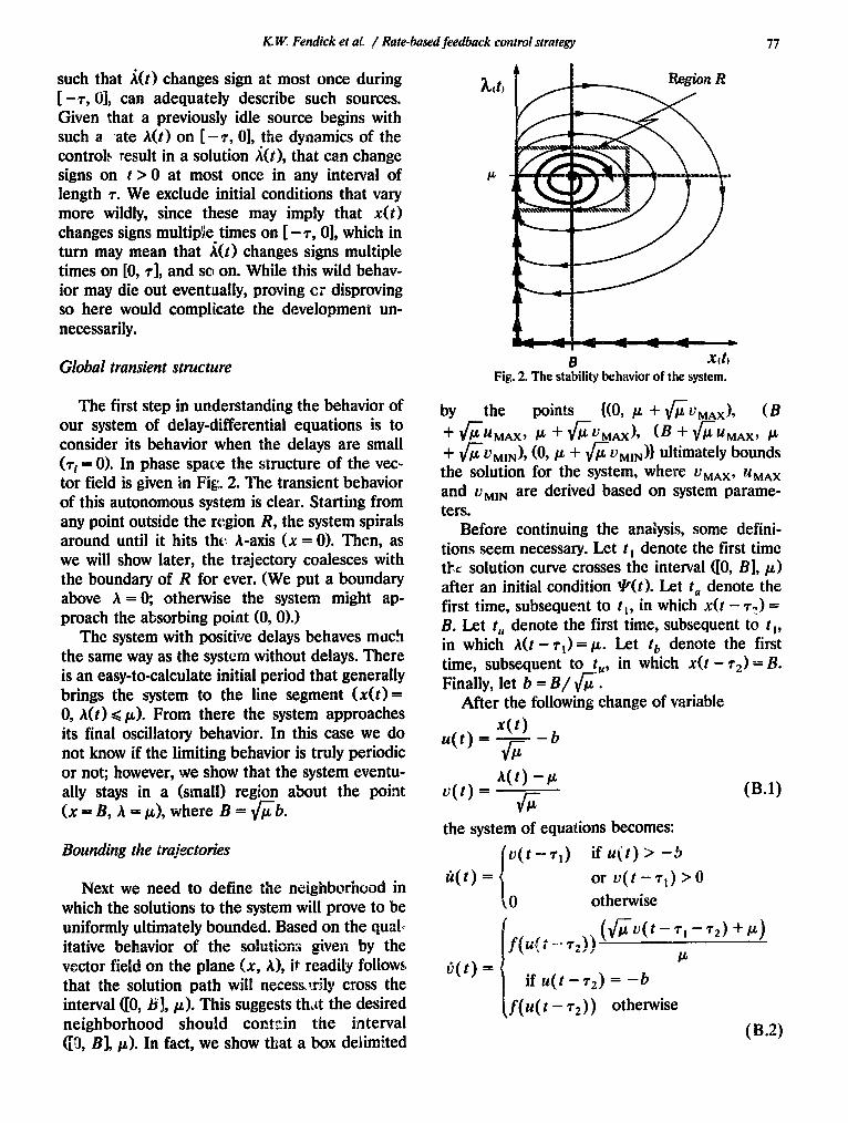
The first step in understanding the behavior of our system of delay-differential equations is to consider its behavior when the delays are small (ri = 0). In phase space the structure of the vector field is given in Fig. 2. The transient behavior of this autonomous system is clear. Starting from any point outside the region R, the system spirals around until it hits tht! A-axis (x = 0). Then, as we will show later, the trajectory coalesces with the boundary of R for ever. (We put a boundary above A = 0; otherwise the system might approach the absorbing point (0, O).)

The system with positive delays behaves much the same way as the system without delays. There is an easy-to-calculate initial period that generally brings the system to the line segment (x(t) = 0, A(t) < p). From there the system approaches its final oscillatory behavior. In this case we do not know if the limiting behavior is truly periodic or not; however, we show that the system eventually stays in a (small) region about the point (x = B, A = p), where B = fib.

Bounding the trajectories

Next we need to define the neighborhood in which the solutions to the system will prove to be uniformly ultimately bounded. Based on the qual- itative behavior of the solutions given by the vector field on the plane (x, A), it readily follows that the solution path will necess,\rfly cross the interval ([0, B], cc). This suggests th& the desired neighborhood should coctein the interval ([O, B], p). In fact, we show that a box delimited

l3 X4 Fig. 2. The stability behavior of the system.

bY the points ((0, cc + fi+,+x), (B + &$#00 P + &JuAx)9 (B + ~4UaX~ CL + fief&, (0, p + &u&) ultimately bounds the solution for the system, where vMAX, idMAX and vMIN are derived based on system parameters.

Before continuing the analysis, some definitions seem necessary. Let t, denote the first time tie solution curve crosses the interval ([0, B], p) after an initial condition !P(t ). Let t, denote the first time, subsequent to t , , in which x(t - r7) = B. Let t,, denote the first time, subsequent to t ,,

in which A(t - 7,) = p. Let t, denote the first time, subsequent to t,,, in which x(t - Q) = B. Finally, let b = B/ 6.

After the following change of variable

v(t) = A(t) -P

4- P

the system of equations becomes:

v( t -- 7,) if u(t) > -5

6(t) = or v(t-7,) >O

0 otherwise

ml)

i

f( i(~i_.72!) (~v(t--T1 -r2) +~)

C(t) = P

if u(t-r2) = -b

If( ( u t - r2)) otherwise

( B-2)

78 K.W. Fendick et al. / Rate-buned fe~'dback control strategy

where f (x ) decreases monotonically oi~ x [ - b , oc] with f ( 0 ) = 0 . Let G(x) denote

fi~(-f(s)) ds.

Bounds for v(to)

Here we find an upper bound and a lower bound for v(t.). Note that

(/z -- ( r , + '~2)¢-~-f ( -b) ) >/

>t

]z

× --r2f(u(: T2))ti(t +~' ,) dt f ta

tl

(/.L- (T I +T2)C--~f(--b)) /x

i:'2(ta) fti"v(t) t'(t)dt= 2

An upper bound can be found in the following way:

× f t . -r~f( u( t))ti( t ) dt l I

(]I,L- (T l " l - T 2 ) ¢ ~ - - f ( - b ) ) f 0 / ( x ) d x ke

,'2(t..) r',,, fti"f'(t)gt(t +r,) dt ~ - - = j. t ( t ) b ( t l dt= il

(I.~ - rl/-~f( - b ) ) G( -b ) . IZ

< f ( - b ) fti"fi(t +r,) dt

= f ( - b ) [ u ( t a + r , ) - u ( t , + r , ) ]

<~f(-b)[(T, +r2)v(t,~ ) + b ] .

The first bound holds since v ( t - ~-)> 0 implies that u(t - r 2) > 0 in the interval t ~ (t,, t~); the second bound follows from tJ <~V(ta). Thus it readily follows that v(t,,) ~ t'MA x, where

!' MAX = r f ( - b ) + C r 2 f 2 ( - b ) + 2 b f ( - b ) . (B.3)

Since b is O(1) as tz -'* o0 and since f does not depend on/z,/,tMA X is O(1) as /z ~ oo.

By the definition of t,, and the dynamics of the equations that govern the system's behavior, we know that v(t~) > 0. We have not found a tighter lower bound for ta that holds generally; but when v(t) has been a, the boundary u(t)= - b for at least an amount of time r 2 before v(t)= 0, we can find a lower bound for t '( t ,) in the following way:

vz(t.) 2 ~ = fti"v(t)i'(t) dt= fti"f'(t)t~(t +rt) dt

The first bound follows from the interval (t~, t a - r 2) being a subset of the interval (t~, ta) combined with the integrand being positive in those intervals; the second bound follows from b(t) ~< f ( - b) in the interval t ~ (t ! - r2, t~); the third bound follows from f(u(t-z2))>~f(u(t)) and ti(t + r ~) >i ti(t) in the interval t ~ ( t ~, t~ - r 2) (here we require that u ( t - z2) be at the boundary in the interval t E (t, , t~ + ~-) and that r~ ~ r2). Thus it readily follows that v(t~) >1 V~A x, where

VMAX'- ~2 (p" -vy/-~f(-b)) G(-b) ( B . 4 )

The function G does not depend on /.~, so that v ~tAX = O(1) as # --* oo.

Bounds for u(t,,)

Here we find an upper bound and a lower bound for u(t,,). Note t 'mt

j.ft"-r'v(t)b(t) d t = v2( tu- ' t l ) v2(ta) t,, 2 2

>i ft~-~b(t)fi(t +r,) dt tl

V2(ta)

K.W. Fendick et aL / Rate-based feedback comrol strategy 79

An upper bound for u(t,,) can be found in the following way:

v2(ta) = - / t " - * i v ( t ) b ( t ) dt

2 t.

" f t " -* '3( t ) f i ( t +'Q) dt d. ta

= f t " - * ' ( - - f ( u ( t - - ¢ 2 ) ) ) t ~ ( t +71) dt

v(t) has been at the boundary u(t)= - b for at least ar~ amount of time ~'2 before ~-~, then v(t.) >t VMA x, and a tighter lower bound for u(t,,) can be found in the following way:

v2(ta)

2 = -/t"-*tv(t)b(t)" dt

d. ta

= f ' " - * '~ ( t )~ ( t +~,) dt ta

= it,, ( - f ( u ( t - ' r , - ' r 2 ) ) ) f i ( t ) dt ta +71

= / t " - " ( - f ( u ( t - - ' r 2 ) ) ) ( t ( t +'r l ) dt ta

= f'" max{0, ( - [ ( u ( t - , , - , 2 ) ) ) } " t a + 1 " I

X~(t) dt

>I (- ,( . , , ,

dt t a + ' r I <~S~I u I ] ]

- ft]"max{O, ( -f(u( t )

- ( ¢ i +~'2)v(ta)))}fi(t) dt

= f ' , , - ' , ( _ : ( . ( , ) - . . ( , o ) ) ) td

X~(t + ~'l) dt

= [ " ( ' " ~ - ' " " ' ~ ( - f ( x ) ) dx "0

= G(u( tu) - "rV( ta) ), where t d is such that U(:a)=¢V(ta). The first bound follows from ( - f ( . ) ) being monotone non-decreasing. Because G(x) --* 0o monotonically as x-- ,®, the equation v2(ta)/2 "-G(t~(t u) -¢v( ta)) has a unique real root. Then if we substitute v(t a) by VMA x the left hand side increases and the right hand side decreases, we find that u(t,) < UMA x, where

V2MAX G(UMAx--ZVMAx) = 2 (B.5)

can be solved for U MA x and an upper bound obtained. Because VMA x is O(1) as /z --* oo, V MAX is also.

By its definition, u(t a) > 0, which is the only lower bound that we know holds in general. If

< ( /d~.(t ,) + ~,)

<~

X - * ' ( - f ( u ( t +'ri)))t~(t +T,) dt / tu

ta

(¢;.(,.) +.)

X/ t ' - r ' ( - f ( u ( t +,rl)))t~(t +,rl) d t t a --71 - -T 2

f t u x ( - f ( , ( t ) ) ) ~ ( t ) dt "ta -~ '2

- + ") - : ( x ) ) P, "o

= + c ( . ( , . ) , ) .

The first bound follows from u(t - ¢2) -<< u(t + ¢ I ) in the interval t ~ (t,. t u -¢2), combined with ( - f ( . ) ) being monotone non-decreasing; the second bound follows from the in*erval (t o, t , ) being a subset of tb~. interval ( t , - r, t ,) combined with the integrand being p~sitlve in those intervals.

Thus, it follows that

V2(ta) G(.(t.)) >~ --~--.

Note that the right hand side: of the above expres- s;on is monotone increasing: with v(t,). There- tore, substituting the lower bound ViA x of V(t o)

80 K W. Fendick et aL / Rate-based feedback control strategy

into the above expression relating u(t.) and v(t a) yields a lower bound UMA x for u(t~):

VM2AX (a .6) G(UMAX) = 2

Because G(x) --, oo monotonically as x - , ~, this has a unique real root /Z~A x, which is O(1) as p- - , ~.

Bounds for V(t b)

Here we find a lower bound and an upper bound for v(tb). Note that

V(tb) 2 v(t)£'( t) d t = -T-" "t u - - 1"1

A lower bound can be found in the following way:

v2(tb) = : ith v ( t ) : : ( t ) dt

2 "t,,-Ti

= + , , ) ) d ,

<~ (-f(u(t,,))) f " (-tJ(t + r,)) dt %,- T I

<~ ( - f ( u ( t . ) ) ) [ u ( t . ) --rV(tb) ] .

The first bound follows from ( - f (u ( t - r2 ) ) )<~ ( - f (u( t . ) ) ) in the interval t ~ ( t . - r e , tb); the second bound follows from ( - t~( t + rl)) ~< (--V(tb)) in the interval t ~ (t b - r2, tb + rl). Thus, it readily follows that

V(tb) >~ - ( - f ( U ( t , , ) ) ) ~ "

- [ ( - f (u(t , , ) ))2r 2

+ 2( - f (u ( t . ) ))u( t .) ] ' /2.

The right hand side of the above expression is monotone non-increasing with U(tu) since its derivative with respect to u(t u) is less or equal to zero. That is,

d

du(t.)

- [ ( - f ( u ( t . ) ) ) r

-¢(-f(u(t.)))2r2 + 2(-f(u(t.)))U(tu) ]

= -(-/,(u(t.))),

--½((--f(U(tu)))2r 2

+2(-f(u(t.)))u(t.))-I/2

X (2(-f(u(t.)))(-f'u(t.)))T + 2 ( - f ' ( u ( t . ) ) ) u ( t . )

+ 2 ( - f ( u ( t . ) ) ) )

<~0 Therefore, substituting the upper bound UMA x for u(t.) into the above expression yields a lower bound VMm for v(tb): UMIN

-- -- (--f(UMAX))T

-- ¢ ( - - f ( U M A X ) ) 2 r 2 + 2( --f(UMAX))UMA x •

(B.7)

Because UMA x is O(1) as ~ ~ oo, VMI N is also. By its definition, v(t b) < 0, which is the only

upper bound that we know holds in general. If v(t) has been at the boundary u ( t ) - - b for at least an amount of time r 2 before tl, then u(t u) >I U~AX, and a tighter upper bound for v(t b) can be found in the following way:

v ( t . ) 2

2

• f b v ( t )~ ( t ) dt -t. - - T !

ffi f b ::( t)(--:~(t + r l ) ) dt -t. - - T I

_ frb ( - - f (u ( t -- r e ) ) ) ( --t~(t + r l ) ) d t -t . 4 - - 1 " 1

( >I (-f(u(t-'2)))(-a(t +'I)) dt - - T ! + 1 " 2

( >I ( - f t u ( t - r 2 ) ) ) ( - a ( t - r 2 ) ) dt - - ' t I + I" 2

ffi f o f ( x) dx "u(t.)

= G ( u ( t . ) ) .

The first bound follows from the interval (t u - r 1 + r 2, t b) being a subset of the interval ( t . - r 1, t b) combined with the , . , . . . o . . a t...;..~ positive in l l l l v ~ & ILl i l ~ i I~ ,~, l l 1 0

K.W. Fendick et aL / Rate-based feedback control strategy 81

those intervals, the second bound follows from ( -u( t + rl)) >t ( -u ( t - I-2)) in the interval t ~ (t~ - :'~ + ¢2, tb). Thus,

V(tb) < -¢2G(u(t , ) )

Note that the right hand side of the above expression is monotone decreasing with u(t,) since its derivative with respect to u(t~) is less or equal to zero:

d du(tu) [ - ¢2G(u(tu)) ]

- ½(2G(u( t~ ) ) ) - ' / 2 (2 ( - f (u ( t~ ) ) ) ) < 0.

Therefore, substituting the lower bound U~AX of U(t~) into the above expression yields an upper bound V~,N for V(tb):

+ = ( B . 8 ) UMIN

Because G does not depend on /~, v ~ N - O ( 1 ) a s / . t --, oo.

Appendix C

Role of the boundary

In Appendix B, we showed, that the solution (x, A) is ultimately bounded by a rectangle delimited by {(0, tt + ¢-~VMAx), (bf~- + V~-UMA x, tt + (bv + V uMAx, + (0,/z ~,-V~--~'MIN)] about the equilibrium po~t (v =b¢~- , a = t t). Even so, the solution cannot converge to the equilibrium point, as the results for 5mall ¢ in Appendix A suggest, where we explored the vector field of (x, A) in the neighborhood of the equilibrium point. In Appendix C, we show that ~he boundary at x - 0 accounts for the boundedness of the solution. We show that no neighborhood of the equilibrium point can bound the solution asymptotically without including the boundary at x ffi 0. Physically, this implies that any solution path within the above rectangle must hit the boundary of the rectangle at x ffi 0. After remaining on the boundary for a while, the solution path will reenter the interior of the rectangle, only to hit the boundary again later. Therefore, the solution path within the rectangle consists of an infinite sequence of excursions away from the boundary and back again. The

, ,

boundary acts to damp the oscillations of the solution.

As in Appendix B, we work with the scaled variables

X(t) u ( t ) = - b

. ( t ) =

and the scaled system (B.2). As we prove below, we only need to consider the system's behavior at times t such that u(s)> -b for s ~ [ t - r 2, t] to prove that the solution (u, v) must keep running into the boundary at u = - b . Then, with the change of variable v,,(t) = v(t - r ! ), the relevant equatfons become

~( t )_[v , , ( t ) i f u ( t ) > - b o r v , , ( t ) > 0

0 otherwise (C.1)

b~,(t) _ f ( u ( t - ¢ ) ) ,

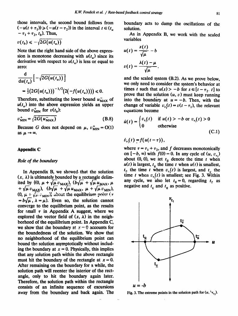
where :- ffi r~ + r 2, and f decreases monotonically on [ - b , 0o) with f(0)ffi 0. In any cycle of (u, v,,) about (0, 0), we let tu denote the time t when u(t) is largest, t~_ the time t when u(t) is smallest, t~ the time t when v~,(t) is largest, and t v the time t when v~,(t) is smallest; see Fig. 3. Within any cycle, we also let tu = 0, regarding t~ as negative and t~ and t~_ as positive.

tv

= /l

U = -b

Fig. 3. The extreme points in the solution path for (u, iv,,).

8 2 K.W. Fendick et al. / Rate-based feedback control strategy

We show instability in regions that do not include the boundary at u = - b through a Lia- punov function V defined for pairs (u, v~,). Let

V(u(t) l '~,(t))- t'~,(t) + G ( u ( t ) ) , (C.2) ' 2

where

~X

G(x) = Jo - f ( z ) dz.

Note that V(0, 0) = 0 and V(u, t,,~) > 0 otherwise. Furthermore, V is convex and increases as l ul increases (with It,,, I fixed) and as Iv~ I increases (with lul fixed).

To show that the solution path cannot remain in any region that excludes the boundary, we must show that the net change in V is positive (and bounded from below) between two successive epochs where (u < 0, t, = 0), unless the solu-

71

tion path hits the boundary at u = -b . At these epochs, u achieves its minimum in a circuit arouad (0, 0), and V = G(u). Therefore, V increases over a cycle beginning and ending with (u < 0, t~,,, = 0) if and only if the minimum value for u over the cycle decreases and moves towards the boundary where u = - b .

We study solution paths within the bounding rectangle from Appendix B (but excluding the boundary at u - - b ) for times t such that u(s) > - b for s ~ I t - r 2, t]. We observe the same re- strictions on initial conditions as in Appendix B. Along such a solution path,

12(u( t ), t,,,( t ) )

= t' 7,( t )[ - f ( u ( t ) ) + t." 7,( t )]

=eT , ( t ) [ - f (u ( t ) ) + f ( u ( t - r ) ) ] , (C.3)

which follows from (C.1) and (C.2). Because u(t) increases when v71(t) > 0 and decreases when t,,~(t)<0, (C.3) shows that V(u(t),v,~(t)) increases everywhere along a solution path, except during one interval immediately following t,, and another immediately following ta. In partff:ular, when t,~,(t)<0, I/(u(t), t,7(xt) ) is negative only between ~= t~ = 0 and t = t such that f(u(D) = f (u (~ - r)). Clearly, ~' < r.

To show that V increases over a cycle, we prove that the increase in V from t = r to t -- ~' + r is greater than its decrease from t = t~ = 0 to t = i', so that the net change in V from t = 0 to

t = i' + I" is positive. Note that ~' + ~" < t,,, since u(i') > 0 by its definition; and u(s) ~< 0 for s [t,_., t,_.-~']. A mirror image of our arguments shows that the net change in V from t,_ to t v also is positive, even though V decreases for a time after t,_,.

Because v 7~(t) decreases monotonically from t = tn = 0 (where L,7~ = 0) to t = t¢ > t + ~',

f i ( l ) (u(t) ,v, , ( t ) ) i s : 0

+ l)(u( t + ,) , vT,( t + , ) )) dt

= , , ( v , , ( t ) [ - f ( u { t ) ) +f(u(t-,-))] i~ ~-

+v,t( t + , ) [ - f ( u ( t + r ) ) + f ( u ( t ) ) ] ) dt

> t ) [ - f ( u ( t + r ) ) + f ( u ( t - r ) ) ] dt,

where v,,(t) < 0 for 0 < t < ~'. If we can show that - f ( u ( - r ) ) > - f ( u ( r ) ) , then clearly - f (u ( t - ,)) > - f ( u ( t + ~-)) for all 0 < t < i'; and the integral on the left of (C.4) (the net increase in V) is positive, as claimed.

By (C.1), I t~,,(t)l increases monotonically from t = t v (where bT, = O) to t = r, since u(t - r ) is nonnegative and increasing over this range. Fur- thermore, ta = 0 lies between t v and ~- with vT,(t a) = O. Therefore,

I v , , ( t ) l > l % ~ ( - t ) l for Itl~< min{ltvl , z}.

(c.s) If t r > -~-, then I v,~(t)l decreases moving back- wards from t = t r to t = - r , but increases moving forwards from t = - t v to t = ~-. Therefore, regardless of whether [t r, I < r or It v [ > ~-,

Iv, ,( t) l > IvT , ( - t ) l for I t l ~<I-. (C.6)

Furthermore, vT~(t)=fi(t) , and u(t) increases monotonically from -~- to 0 and decreases monotonically from 0 to r. Therefore, (C.6) implies that u(0) - u(~-) > u(0) - u ( - - r ) , i.e., u(~-) < u ( - 7 ) . Then, because - f increases monotonically, we conclude that - f ( u ( ~ - ) ) < - f ( u ( - ¢ ) ) , which completes the proof that the net change in V over a cycle is positive.

To prove that u(t) must eventually hit the boundary u(t)-- -b , it remains to show that the positive change in V(u(t), v,~(t))over a cycle is

K.W. Fendick et aL / Rate-based feedback control strategy 83

bounded from below. To do so, we bound the (positive) increase in V from t,~ to t,, from below. Note that any increase in V over this range is a net increase in V over the cycle. Let

g(t,._., t,_,) - sup { - f ( u ( t ) ) + f ( u ( t - - ¢ ) ) } . t~[t~,t u]

This quantity is negative. By (C.3)

V(u(t,_,), o~,(t~_))-- V(u(tt), v~,(tt))

- fli'-'l?(u( t ), o,,( t ) ) dt

• r t u

>~ g( t,,, tu) Jt,-Vr,( t ) dt

= g( t,_,, t,_,)[ u(tu) - u( t~)] > o. (c.7)

Our previous arguments have shown that the solution cannot converge to (0, 0) as t ~ ®, so that g(t,:, t,_)[u(t.)-u(t~_)] in (C.7) cannot approach zero in successive cycles as t -~ oo.

Appendix D

Proof of Theorem 4

We now consider a modification of our basic equations:

t ) =

if A ( t - ¢,) - / z > 0

or x( t ) > 0 otherwise

(D.1)

d ~-~A(t) = G ( x ( t - ' r 2 ) , A ( t - t , - r2 ) , A(t), Iz).

(D.2)

We assume that there is a positive constant C such that

I f ( x ( t - T2) )A( t -- T, -- 1"2)

- G ( x ( t - ¢ 2 ) , A ( t - - ' r 2 - - T 2 , A ( t ) , //,))

c1/r~ (D.3)

and that the global transient behavior is pre- served.

We scale the system to (u, v) as in Appendix B; here, the difference between f and g is bounded by a constant independent of /z , where

f = F~ ¢-~ and g = G~ ¢--~. Hence, observing the evolution of the solution paths starting from an arbitrary point and integrating (D.3) in an interval of length t, it follows that

I (U,V)c( t ) - - (U,V)F(t ) I ~Ct.

Let t* be the time it takes (u, v) F to complete a circuit of the origin (this time is easily seen to be independent of the radius, so long as the radius is O(1)). We have t*(/~)= O(1) as /~ ~ ® , so the G-system again has an O(1) bounding box in one orbit. Now the global structure comes into play, allowing us to piece together the local estimates into a global one: Once we have x(t)ffi 0, the system is forced to shrink again to a small neighborhood of the operating point.

References

[1] J.C. Bolot and A.U. Shankar, Dynamic behavior of rate- based flow control mechanism, ACM SIGCOMM Corn- put. Comm. Rev. 30 (1990)35-49.

[2l A.E. Eckberg, D.T. Luan and D.M. Lucantoni, Band- width management: a congestion control strategy for broadband packet networks: characterizing the throughput-burstiness filter, Proc. ITC Specialist Seminar, Adeleide, Australia, 25-29 September 1989; also pub- iished in Comput. Networks ISDN Systems 20 (1990) 415-423.

[3] E.M. Gafni and D.P. Bertsekas, Dynamic control of session input rates in communication networks, IEEE Trans. Aurora. Control 29(11)(1984).

[4] M. Gerla and L. Kleinrock, Flow control: a comparative survey, IEEE Trans. Comm. 28(4)(1980).

[5] E.L. Hahne, C.R. Kalmanek and S.P. Morgan, Fairness and congestion control on a large ATM data network with dynamically adjustable windows, 13th International Teletraffic Conference, July 1991.

[6] J. Hale, Theory of Functional Differential Equations (Springer, Berlin, 1977).

[7] M.W. Hirsch and S. Smale, Dtfferential Equations, Dy- namical System, and Linear Algebra (Academic Press, New York, NY, 1974).

[8] E. Isaacson and H.B. Keller, Analysis of Numerical Meth- ods (Wiley, New York, NY, 1966).

[9] V. Jacobson, Congestion avoidance and control, Proc. ACM SIGCOMM'88, August 1988, pp. 314-329.

[10] R. Jain, A timeout-based congestion control scheme for window flow-controlled networks, IEEE J. Selected Areas Comm. 4(7) (1986) 1162-1167.

[11] S. Keshav, Congestion control in computer networks, Dissertation, University of California at Berke, ley, August 1991.

[12] D. Mitra, Asymptotically optimal design of congestion control for high speed data networks, IEEE Trans. Comm. 40(2) (1992) 301-311.


[13] D. Mitra and J. Seery, Dynamic adaptive windows for high speed data networks: theory and simulations, Proc. ACM SIGCOMM'90, August 1990, pp. 20-30.

[14] D. Mitra and J.B. Seery, Dynamic adaptive windows for high speed data networks with multiple paths and propagation delays, Proc. IEEE INFOCOM'91, Bal Harbour, FL, April 1991, pp. 2B.l.l-2B.1.10.

[15] D. Mitra, I. Mitrani, K.G. Ramakrishnan, J.B. Seery and A. Weiss, A unified set of proposals for control and .desi~, of h'.'g~a speed data networks, Queueing Systems 9 (1991) 215-234. -

[16] A. Mukherjee and J.C. Strikwerda, Analysis of dynamic

congestion control protocols--a Fokker-Planck approximation, Proc. ACM SIGCOMM'91, August 1991, pp. 159-169.

[17] K.K. Ramala'ishnan and R. Jain, A binary feedback scheme for congestion avoidance in computer networks with a connectionless network layer, Proc. ACM SIG- COMM'88, August 1988, pp. 303-313.

[18] M. Reiser, A queueing network analysis of computer communication networks with window flow control, IEEE Trans. Comm. 27(8) (1979) 1199-1209.

[19] T. Yoshizawa, Stability Theory by Liapunov's Second Method (Math. Soc. Japan, 1966).

Analysis of a rate-based feedback control strategy for long haul data transport

Documents

Transcript of Analysis of a rate-based feedback control strategy for long haul data transport