Analysing extensive fish culture systems by transparent population modelling: bighead carp,...

Aquaculture Research, 1997, 28, 867–880

Analysing extensive fish culture systems by

transparent population modelling: bighead carp,

Aristichthys nobilis (Richardson 1845), culture in a

Chinese reservoir

K LorenzenRenewable Resources Assessment Group, Imperial College, University of London, London, UK

G Xu, F Cao, J Ye & T HuZhejiang Institute of Freshwater Fisheries, Huzhou, Zhejiang Province, China

Correspondence: K Lorenzen, RRAG, Imperial College, 8 Princes Gardens, London SW7 1NA, UK (e-mail: [email protected])

Abstract

A transparent population modelling approach isused to analyse a large-scale extensive fish culturesystem, the bighead carp, Aristichthys nobilis(Richardson 1845), fishery in a Chinese reservoir.The population model incorporates explicit sub-models for density-dependent growth and size-dependent mortality, and allows the assessment ofstocking density, seed fish size, fishing mortality(fishing effort), and gear selectivity. The processof model building and parameter estimation fromstocking and catch data is described in detail. Thefull analysis is carried out in computer spreadsheetswhere all model components are visible and caneasily be modified to take account of specificconditions, or to explore different assumptions. Thepractical use of the model in management decisionmaking is discussed, together with data requirementsand the possible need for experimental management.

Introduction

In extensive aquaculture seed fish are stocked, leftto utilize natural aquatic production for growth,and recaptured upon reaching a desired size.Management in extensive culture is thus concernedwith the development of stocking and harvesting

© 1997 Blackwell Science Ltd. 867

regimes that make efficient use of a given naturalproductivity. Quantitative analysis and modelling ofthe culture system can aid management decisionmaking in two ways: the process of analysis improvesthe understanding of the interactions betweenmanagement actions and natural processes, and thederived model may be used to evaluate differentmanagement options. To realize this potential, theanalysis and modelling framework must betransparent and flexible to allow constructiveinteraction between decision makers and analysts.This paper describes the process of analysing andmodelling a large-scale culture system in a Chinesereservoir, using a spreadsheet-based transparentpopulation model.

Extensive fish culture in Dongfengreservoir, China

Extensive fish culture is a widespread practice inChinese reservoirs and lakes, with a total productionestimated at 0.3–0.6 million t year–1 (Lu 1992;Wang & Li 1995). The culture system analysedin the present study operates in a multi-purposereservoir in Zhejiang Province, in the temperateregion of China. Dongfeng is a medium-size reservoirwith an average surface area of 100 ha and amean depth of 7 m. Managed comprehensively by

Analysing extensive fish culture systems K Lorenzen et al. Aquaculture Research, 1997, 28, 867–880

a reservoir bureau, Dongfeng is used for extensivecarp culture in a common Chinese system describedby De Silva, Yu & Xiang (1991) and Li & Xu (1995).The reservoir is stocked around the end of eachyear with large (12 cm) fingerlings of bighead carpAristichthys nobilis (Richardson 1845), silver carpHypophthalmichthys molitrix (Cuvier & Valenciennes1840), and small numbers of other carp species.Harvesting takes place only once a year aroundDecember and January, using the ‘combined fishingmethod’. In the combined method, seine nets andblocking nets are used to drive fish into a largestationary trap net. Only fish of marketable size areharvested, selected by the gear but also by hand.The total production from Dongfeng reservoir isabout 750 kg ha–1 year–1, comprising 60% bigheadcarp, 32% silver carp, and 8% other carp species.Bighead and silver carp do not reproduce naturallyin the reservoir, and their yield is based entirely onregular stocking.

The present management regime of Dongfengreservoir was established in an experimental studyconducted from 1974 to 1978. During theexperiment, stocking densities were increased overprevious levels and stabilized at a total 2700 ha–1

year–1, with 1700 ha–1 year–1 of bighead carpfingerlings. The age distribution and weight at ageof fish in the catch were determined regularly, andthe number and body weight of seed fish recorded.These data are used here to illustrate the process ofmodel development and analysis. The managementof Dongfeng reservoir has not changed greatly sincethe experiment, but no detailed data have beencollected since 1978.

Analysis and model development

The population dynamics of fish in extensive cultureare determined by the management actions ofstocking and harvesting, in interaction with thenatural processes of individual growth and mortality.Lorenzen (1995) developed a size-structuredpopulation model for culture-based fisheries andextensive fish culture, incorporating explicit sub-models for the processes of density-dependent growthand size-dependent mortality. In the present paperthe model is reformulated in an age-structuredframework. The model is implemented in computerspreadsheets, together with tools for the estimationof model parameters from stocking and catch data.

The individual growth of fish is described by a

868 © 1997 Blackwell Science Ltd, Aquaculture Research, 28, 867–880

density-dependent version of the von Bertalanffygrowth function (VBGF), described in Lorenzen(1996a). In the model, asymptotic weight W`B isdefined as a function of population biomass:

W`B 5 (W1/3`r – c (B – Br))3 (1)

where B is the actual population biomass, W`r isthe asymptotic weight at reference biomass Br, andc is the competition coefficient which describesthe decline in asymptotic weight with increasingbiomass. Mortality is described by a power functionof weight in accordance with theoretical andempirical studies of fish mortality (Peterson &Wroblewski 1984; McGurk 1986; Gulland 1987;Lorenzen 1996b):

W b (2)Mw 5 Mr ( )

Wr

where MW is the natural mortality rate at weightW, Mr is the mortality rate at reference weight Wr,and b is the allometric scaling factor of naturalmortality.

The analysis of the fish culture system is conductedin four steps. First, cohort analysis is used to estimatefishing and natural mortality rates, and toreconstruct the population biomass dynamics overthe period of the experiment. Second, the informationon biomass dynamics is used to estimate parametersof the density-dependent growth model. Third, asize-based selectivity model is fitted to predict theeffects of density-dependent growth on fishingmortality rates. Finally, an equilibrium yield modelis constructed and used to predict the response ofthe culture system to changes in stocking andharvesting patterns. All analyses are carried out incomputer spreadsheets which are illustrated inTables 1, 2 and 3. Details of the spreadsheetconstruction and analysis procedures are given inthe Appendix.

Cohort analysis

The reconstruction of the population and estimationof mortality rates is conducted by means of cohortanalysis (also known as virtual population analysis,for a general account see Hilborn & Walters 1992).Cohort analysis reconstructs individual cohorts (yearclasses) of fish from the catches taken from thatcohort over its lifetime. The analysis starts at theterminal age group of the cohort, i.e. the last agegroup that has contributed to the catch. Terminal

Aquaculture Research, 1997, 28, 867–880 Analysing extensive fish culture systems K Lorenzen et al.

Table 1 Cohort analysis spreadsheet for bighead carp in Dongfeng reservoir (experiment 1974–78)

A B C D E F G H

1 Cohort analysis for extensive fish culture23 Year Age (years) 0 1 2 3 445 Body weight (g)67 1974 15 355 655 3150 52508 1975 15 265 960 1320 40509 1976 15 235 635 2190 3090

10 1977 15 190 655 1410 332011 1978 15 175 665 1075 20901213 Catch (ha–1)1415 1974 0.0 61.2 340.0 7.6 0.316 1975 0.0 61.9 161.0 158.9 0.317 1976 0.0 8.8 175.0 47.4 14.518 1977 0.0 19.0 231.0 90.6 9.819 1978 0.0 1.0 121.0 169.7 5.92021 Population (ha–1)22 Stocking No.23 1974 850 865.3 387.9 576.4 8.0 0.324 1975 1407 1437.7 494.8 238.8 179.7 0.325 1976 1715 1748.9 810.2 305.2 61.2 16.826 1977 1554 1574.4 959.9 563.1 99.2 11.327 1978 1703 1703.0 855.2 655.7 250.1 6.82829 Natural mortality30 b 5 –0.331 Mr 5 0.27 year–1

32 Wr 5 1000 g3334 Fishing mortality (year–1)

Average 3,43536 1974 0.000 0.172 0.891 2.956 2.000 2.47837 1975 0.000 0.134 1.121 2.155 2.000 2.07838 1976 0.000 0.011 0.852 1.487 2.000 1.74439 1977 0.000 0.020 0.528 2.447 2.000 2.22440 1978 0.000 0.001 0.204 1.135 2.000 1.56841 Average 1974–78 0.000 0.067 0.719 2.036 2.0004243 Population biomass (kg ha–1)44 Total45 1974 554 13 137 377 25 246 1975 619 22 130 229 237 147 1976 594 26 189 193 134 5248 1977 750 24 181 368 140 3849 1978 894 26 149 436 269 14

© 1997 Blackwell Science Ltd, Aquaculture Research, 28, 867–880 869


Table 2 Spreadsheet layout for the estimation of growth parameters. Parameters have been estimated by minimizing thesum of squared differences (SSQ) between the observed and expected weights

A B C D E F G H

1 Estimation of density-dependent VBGF parameters23 Year Age (years) 0 1 2 3 445 Observed weights (g)67 1974 15 355 655 3150 52508 1975 15 265 960 1320 40509 1976 15 235 635 2190 3090

10 1977 15 190 655 1410 332011 1978 15 175 665 1075 20901213 Model parameters1415 W`r 5 10525 g16 K 5 0.20 year–1

17 c 5 0.012 g1/3 ha kg–1

18 Br 5 714 kg ha–1

1920 Predicted weights (g)2122 B (kg ha–1) W`B (g)23 197424 1975 619 12194 234 985 1430 422325 1976 594 12661 240 847 1854 229526 1977 750 9935 205 712 1302 306027 1978 894 7822 175 569 1223 208228 Average 7142930 Squared differences of the log transformed observed and expected weights3132 197433 1975 0.0028 0.0001 0.0012 0.000334 1976 0.0001 0.0157 0.0052 0.016735 1977 0.0010 0.0013 0.0012 0.001336 1978 0.0000 0.0046 0.0031 0.00003738 SSQ 5 0.055

age groups are the oldest age groups in cohorts thatno longer contribute to the catch, and all theage groups in the most recent year included inthe analysis.

In Dongfeng, fishing mortality occurs in a singleannual event (during which natural mortality isnegligible), while natural mortality acts throughoutthe year. Hence the number of fish alive in theterminal age group prior to fishing equals thenumber caught, divided by the proportion of fish


harvested. If the proportion harvested is expressedas an exponential fishing mortality rate Fa,t, thenthe terminal numbers alive Na,t (at age a and timet) are given by

Ca,t (3)Na,t 5

1 – exp(–Fa,t)

where Ca,t is the terminal catch. The younger agegroups in the cohort are reconstructed by successivelyworking backwards from the terminal group. The


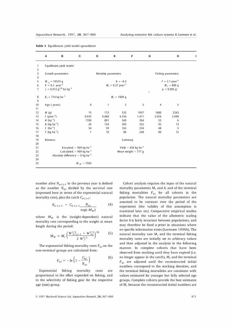
Table 3 Equilibrium yield model spreadsheet

A B C D E F G H I

1 Equilibrium yield model23 Growth parameters Mortality parameters Fishing parameters45 W`r

5 10525 g b 5 –0.3 F 5 2.1 year–1

6 K 5 0.2 year–1 Mr 5 0.27 year–1 Wc 5 880 g7 c 5 0.012 g1/3 ha kg–1 p 5 0.005 g–

1

8 Br 5 714 kg ha–1 Wr 5 1000 g9

10 Age ( years) 0 1 2 3 4 51112 W (g) 15 173 533 1057 1680 234313 F (year–1) 0.033 0.068 0.334 1.471 2.056 2.09814 N (ha–1) 1700 891 569 304 55 615 B (kg ha–1) 26 154 303 322 92 1316 C (ha–1) 54 59 162 234 48 517 Y (kg ha–1) 1 10 86 248 80 121819 Biomass Summary2021 Assumed 5 909 kg ha–1 Yield 5 436 kg ha–1

22 Calculated 5 909 kg ha–1 Mean weight 5 777 g23 Absolute difference 5 0 kg ha–1

2425 W`B 5 7503

number alive Na-1,t-1 in the previous year is definedas the number Na,t divided by the survival rate(expressed here in terms of the exponential naturalmortality rate), plus the catch Ca-1,t-1:

Na,t (4)Na–1,t–1 5 Ca–1,t–1

exp(–MW)

where MW is the (weight-dependent) naturalmortality rate corresponding to the weight at meanlength during the period:

W1/3a–1,t–1 1 W1/3

a,t3b (5)

MW 5 Mr ( )2 W1/3

r

The exponential fishing mortality rates Fa,t on thenon-terminal groups are calculated from:

Ca,t (6)Fa,t 5 – ln ( 1 – )

Na,t

Exponential fishing mortality rates areproportional to the effort expended on fishing, andto the selectivity of fishing gear for the respectiveage (size) group.


Cohort analysis requires the input of the naturalmortality parameters Mr and b, and of the terminalfishing mortalities Fa,t for all cohorts in thepopulation. The natural mortality parameters areassumed to be constant over the period of theexperiment (the validity of this assumption isexamined later on). Comparative empirical studiesindicate that the value of the allometric scalingfactor b is fairly invariant between populations, andmay therefore be fixed a priori in situations whereno specific information exists (Lorenzen 1996b). Thenatural mortality rate Mr and the terminal fishingmortality rates are initially set to arbitrary valuesand then adjusted in the analysis in the followingmanner. In complete cohorts that have beenobserved from stocking until they have expired (i.e.no longer appear in the catch), Mr and the terminalFa,t are adjusted until the reconstructed initialnumbers correspond to the stocking densities, andthe terminal fishing mortalities are consistent withvalues estimated for younger but fully selected agegroups. Complete cohorts provide the best estimatesof Mr because the reconstructed initial numbers are


insensitive to the assumed terminal Fa,t. Expiredcohorts that have been observed only during theirlater years are reconstructed in a similar way, usingthe Mr estimate from the complete cohorts. In activecohorts which contribute to the catch in the mostrecent year, terminal Fa,t assumptions have a majorimpact on the reconstructed numbers and thereforerequire careful consideration. Terminal Fa,t valuesmay be set to correspond to the values estimatedfor the same age group in previous years, assumingthat fishing mortality at age has remained constantover time. Alternatively, terminal fishing mortalitiesmay be set so that reconstructed initial numberscorrespond to stocking densities, allowing fishingmortalities to vary over time. If the two approacheslead to different results, then either fishing or naturalmortality rates have changed over time, and furtherinformation and judgement are necessary to decidewhich is the case. If the question cannot be resolved,both assumptions should be carried through the fullanalysis, including the assessment of managementoptions.

Once all cohorts have been reconstructed, totalpopulation biomass Bt in year t is calculated as:

Bt 5 Σamax

a 5 0

Na,t Wa,t (7)

Statistical confidence limits for results of the cohortanalysis are difficult to obtain due to the use ofexternal information and subjective judgement, andit is therefore important to assess the sensitivity ofresults to different assumptions. Erroneousassumptions lead to systematic errors which cannot be detected by statistical analyses, while randomvariation in fishing mortality is reflected in Fa,t

estimates and can be quantified by fitting a selectivitymodel as described later.

Growth model estimation

The density-dependent VBGF predicts the meanindividual weight Wa,t as a function of Wa-1,t-1 (thecohort’s mean individual weight in the previousyear), and of W`B:

Wa,t 5 ((W1/3`B – (W1/3

`B – W1/3a–1,t–1) exp( – K))3 (8)

The asymptotic weight W`B is a function ofpopulation biomass as defined in equation 1. It isassumed here that the weights Wa,t in year t reflectthe population biomass Bt at the same instantin time.


If weight at age data are available and thepopulation biomass dynamics have beenreconstructed, then the parameters of the density-dependent VBGF can be estimated as follows. Foreach observed weight Woa-1,t-1, the predicted weightWpa,t in the following year is calculated fromequation 8, subject to Bt. The best estimates ofthe growth model parameters are the values thatminimizes the sum of squared differences (SSQ)between the observed and expected weights, Woa,t

and Wpa,t. Applying a logarithmic transformation,the SSQ is calculated as

SSQ 5 Σamax, tmax

a 5 0, t 5 tmin

(log(Woa,t) – log( Wpa,t))2 (9)

The parameter set that minimizes SSQ is foundby numerical search, as described in the Appendix.Approximate confidence limits for the estimates aregiven by the parameter values that satisfy

SSQ(W`r, K, c) 5

3 (10)SSQ(W`r, K, c) ( 1 1 F(3,n – 3,1 – q) )

n – 3

where W`r, K and c are the best estimates, and F isthe value of the cumulative F-distribution for nobservations and significance level q (Draper & Smith1981). These confidence limits are approximateand may underestimate the true uncertainty inparameter values for two reasons. Most data pointsoccur twice, in the independent and in the dependentvariable, which may lead to bias in both the pointand variance estimates of parameters. Also, thereconstructed biomass may be subject to systematicerrors which are not reflected in the confidencelimits of the growth model parameters. Nevertheless,the derived confidence limits provide a usefulindication of the uncertainty in parameter estimatesand their approximate nature can be accounted forby using wider limits in the uncertainty analysis ofmanagement options.

Selectivity model estimation

In the cohort analysis, fishing mortality has beentreated as an age-related parameter. However, fishare selected for harvesting by size not age, anddensity-dependent changes in growth lead tochanges in fishing mortality at age. It is thereforenecessary to express F as a function of individualweight, here in the form of a logistic relationship:


F9t (11)Fa,t 5

1 1 exp(p (Wc – Wa,t)

where F9t is the fishing mortality on the fully selectedsize-groups, Wc is the mean selection weight, and pindicates the steepness of the logistic curve.Selectivity parameters are estimated analogous togrowth parameters, by determining the values thatminimize the SSQ between the Fa,t-values determinedin the cohort analysis and the values predicted byequation 11. Approximate confidence limits can bedetermined in the same way as for the growth modelparameters.

Equilibrium yield prediction, sensitivity anduncertainty analysis

At equilibrium, population structure, biomass andyield are constant and independent of time, anda cross-section of the population is equivalent tofollowing a cohort over its lifetime. Equilibrium yieldis calculated by following a cohort of stocked fishover its lifetime, using the growth and mortalityequations derived above. A complication arisesbecause growth is dependent on biomass, which inturn depends on growth. Hence the equilibriumpopulation structure is found by solving the equation

B*5 Σamax

a 5 0

N(B*)a W(B*)a (12)

for the equilibrium biomass B* subject to the modelparameters, and the stocking density and bodyweight of seed fish (N0 and W0, respectively). Thepopulation N(B*)a at age is given by

N(B*)a 5 N(B*)a–1 exp(– Fa–1) exp(– MW) (13)

where Fa–1 is the fishing mortality rate defined as alogistic function (equation 11) of weight W(B*)a–1.The natural mortality rate MW is given byequation 5. Weights W(B*)a are given by equation 8,with W`B defined by equation 1.Once the equilibrium population has been found bysolving equation 12, the corresponding catches Ca

are calculated from:

C(B*)a 5 N(B*)a (1 – exp(– Fa)) (14)

Total equilibrium yield Y* is then:

Y*5 Σamax

a 5 0

C(B*)a W(B*)a (15)

The model does not necessarily have an


equilibrium solution for all possible parameter valuesand conditions, but in general a solution exists for theparameter values and conditions of practical interest.

An uncertainty analysis is carried out on theabsolute level of equilibrium yield, as well as on therelative response in yield to changes in management.The analysis identifies key uncertainties which mustbe considered in the analysis of management options.

Results

All analyses were carried out using a priori valuesfor the allometric exponent of natural mortality bconsistent with the empirical results of Lorenzen(1996b). The standard value of b was set at –0.3,while values of –0.2 and –0.5 were used in orderto assess the uncertainty in predictions resultingfrom the uncertainty about the true value of b forthe population.

Cohort analysis

The cohort analysis spreadsheet with the finalresults of the analysis is shown in Table 1 (seethe Appendix for details of implementation). Thenatural mortality rate at reference weight Wr 5

1000 g has been estimated as Mr 5 0.27 year–1,given the standard value of b 5 –0.3. The naturalmortality rates for the other assumed values of bare Mr 5 0.32 year–1 for b 5 –0.2, and Mr 5

0.19 year–1 for b 5 –0.5. Terminal fishing mortali-ties in the active cohorts have been adjusted sothat their initial numbers correspond to the knownstocking densities, allowing for changes in Fa,t

over time. The estimated Fa,t rise steeply from age0 to 3 years, reflecting the increasing selectionby the fishing gear. Over time, fishing mortalitiesin ages 3 and 4 years are relatively stable, whilethere is a sharp decline in F at age 1 year, andto a lesser extent at age 2 years. The actual andreconstructed stocking numbers are shown inFig. 1, for the estimated rate of natural mortalityand a 10% variation in this rate. Also shown arethe stocking numbers obtained by setting theterminal Fa,t values to their averages over thepreceding years. Stocking numbers reconstructedusing this criterion are far below the actualnumbers in 1976 and 1977, indicating that Fa,t

must have changed over time as described above.The decline in reconstructed stocking numberscould also be attributed to an increase in natural


Figure 1 Actual and reconstructed initial cohort densitiesduring the experiment. The actual stocking densities aredenoted by squares. The solid line indicates initial cohortdensities obtained by adjusting the terminal Fa,1978 toreconstruct actual stocking densities. Dotted lines indicatethe sensitivity of reconstructed initial densities to a 10%variation in the natural mortality rate Mr. The dashed lineindicates initial cohort densities obtained by setting theFa,1978 to the average Fa,1974–78.

mortality rates to 0.58 year–1 in the 1976, and2.2 year–1 in the 1977 cohorts. However, suchan increase in Mr would imply reduced yields inthe years following the experiment, which is notborne out in the actual data (cf. Fig 5). Hencedeclining fishing mortality in the younger agegroups due to density-dependent growth reductionis the most plausible explanation of the observedpatterns. This is also supported by the results offitting the weight-based selectivity model (seebelow).

The population biomass is dominated by ages 1to 3. The reconstructed total biomass is shown inFig. 2, for the different assumed values of b. Biomassrises sharply (from about 550 to 900 kg ha–1) overthe period, particularly after 1976 when the strongcohorts stocked from 1975 onwards have reachedsignificant biomass (Table 1). The assumed value ofb has only a minor influence on the absolute levelof the reconstructed biomass, and even less impacton the relative change in biomass over time.

Growth model estimation

The spreadsheet used for growth model estimationis shown in Table 2. Based on the biomassreconstruction for b 5 –0.3, the density-dependentgrowth parameters, together with their approximate


Figure 2 Reconstructed biomass of bighead carp duringthe experiment. The solid line indicates biomass for thedefault value of b 5 –0.3. Also shown are the results forb 5 –0.5 (dashed line) and b 5 –0.2 (dotted line).

Figure 3 Observed (solid lines) and predicted (heavy solidlines) weights at age 1 (j), 2 (m), 3 (.) and 4(d) yearsduring the period of the experiment. Predictions representthe best fit of the growth model (Table 2).

95% confidence limits (in brackets) are W`r 510525(7530, 14700) g, K 5 0.2 (0.17, 0.23) year–1 andc 5 0.012 (–0.009, 0.031) g1/3 ha kg–1, for areference biomass of Br 5 714 kg ha–1 (the averagebiomass in 1975–78). The same set of growthparameters is estimated using the biomassreconstructions for other values of b when thereference biomass is set to the respective averages(Br 5 732 kg ha–1 for b 5 –0.2 and Br 5 684 forb 5 –0.5). The observed and predicted weight atage over the period are illustrated in Fig. 3. Theapproximate confidence limits of the competitioncoefficient c are very wide, and include negativevalues. Negative values of c imply a positive effectof population density on growth, which contradictsbiological knowledge and management experience.


Figure 4 Fishing mortality Fa,t patterns estimated in thecohort analysis; (a) Fishing mortality at age in differentyears, (b) Fishing mortality in relation to weight, with thefitted weight-dependent selectivity model (heavy solid line).The different years are denoted by symbols (j) 1974 (m)1975 (.) 1976 (d) 1977 (.m) 1978.

Hence in the analysis of management options, c 5

0 is considered the lowest possible value. (If negativedensity-dependence is strongly apparent in theanalysis, this may indicate a change in W`r overtime which would require a structural alteration inthe model.)

Selectivity model estimation

The spreadsheet used to estimate the selectivitymodel parameters is similar to that used for thegrowth model, and is not shown here. The selectivityparameters with approximate 95% confidence limitswere estimated as F 5 2.1 (1.8, 2.4) year–1, Wc 5

880 (700, 1080) g, and p 5 0.0048 (0.0026,0.0100) g–1. An overview of the Fa,t patternsreconstructed in the cohort analysis is given inFig. 4a, while Fig. 4b shows the reconstructedfishing mortalities in relation to weight, togetherwith the fitted selectivity model. The reconstructed


fishing mortalities are well described by the weight-based selectivity model.

Equilibrium yield predictions

The yield model spreadsheet is reproduced in Table 3,showing the equilibrium solution for the bestparameter estimates and the end of experimentmanagement regime. The equilibrium biomass is909 kg ha–1, and the equilibrium yield is 436 kg ha–1

year–1 with an average body weight of 777 g.Catches and yield are dominated by fish of age 3years, hence the production cycle of the culturesystem is effectively 3 years. The mortality andgrowth parameters derived for alternative values ofb (–0.2 and –0.5) result in the same equilibriumyield as the standard set, albeit at slightly differentvalues of equilibrium biomass.

The actual stocking density and yield of bigheadcarp in Dongfeng reservoir from 1974 to 1980 areshown in Fig. 5, together with the stocking densityand predicted yield of the end-of-experimentequilibrium solution. Stocking density has beenapproximately 1700 ha–1 per year since 1976, andthe actual yield approaches the predicted equilibriumyield 3 years later, in 1979. Equilibrium modelpredictions correspond well to the observed yield.

The results of the uncertainty analysis of yield andyield response to changes in management (50%reduction in stocking density, 50% reduction infishing mortality, and 67% reduction in fingerlingbody weight) are given in Table 4. The parameteruncertainties are based on the approximateconfidence intervals for growth and selectivityparameters, and on external information and criticaljudgement for the natural mortality parameters.Uncertainty in b is based on the comparative studyof Lorenzen (1996b), while uncertainty in Mr wasdetermined by assuming a maximum error of 20%in the recorded stocking data and calculating thecorresponding error in Mr. The single-most uncertainparameter is the competition coefficient c, followed bythe steepness parameter p of the selectivity model.Overall, the predictions are fairly insensitive tovariation in parameters; all parameter uncertaintiesresult in smaller relative uncertainties in the yieldpredictions. The growth parameters are the greatestsource of uncertainty about the absolute value ofyield, and the competition coefficient c is by far thegreatest source of uncertainty in the yield response tochanges in management. The analysis of


Table 4 Uncertainty analysis of the equilibrium yield model. Given are the uncertainty in parameter values and thecorresponding sensitivity of predicted yield and yield response to changes in management. The alternative managementscenarios are a 50% reduction in fishing mortality (F 3 0.5), a 50% reduction in stocking density (SD 3 0.5) and a 67%reduction in the weight of seed fish (W0 3 0.33).

Sensitivity of relative change in yield (%) due to

Uncertainty Sensitivity ofParameter % yield (%) F 3 0.5 SD 3 0.5 W0 3 0.33

W`r 35 19 4 2 0K 16 14 2 3 2c 130 22 28 34 12b 55 9 10 6 7Mr 23 9 6 5 3F 15 2 5 3 2Wc 22 5 10 11 4p 80 9 7 9 4

Figure 5 Stocking density (dashed line) and yield (solidline) during the experiment and the following two years.Lines with solid squares indicate the actual values. Thecorresponding horizontal lines without symbols indicatethe end-of-experiment density, and predicted equilibriumyield.

management options must therefore account foruncertainty primarily with respect to the value of c.

Analysis of management options

The equilibrium solution of the model for the standardparameter set and end-of-experiment conditions wasused as a benchmark for the evaluation ofmanagement options. This benchmark solution(which corresponds well to the observed yield after1978; Fig. 5) was treated as known, and madeindependent of the value of c by setting the reference


biomass and corresponding asymptotic weight of thegrowth model to the equilibrium values.

The predicted responses in yield to changes instocking density and fishing mortality are shown inFig. 6, for the standard value of c 5 0.012 g1/3 hakg–1 and the extreme values of c 5 0 g1/3 ha kg–1 andc 5 0.031 g1/3 ha kg–1. Arrows indicate the status atthe end of the experiment. The analysis indicates thatthe end-of-experiment stocking and harvestingregimes are near optimal, unless the true value of c isvery different from the best estimate.

The predicted effect of changing the body weightof stocked fingerlings is shown in Fig. 7, for thestandard and extreme values of both c and b.Uncertainty in c has a greater overall effect onpredicted yield than uncertainty in b. For the bestestimate of c, yield is fairly insensitive to fingerlingweight. In the absence of density dependence, areduction in fingerling weight would result in amore marked loss of yield. Under extremely highdensity dependence, a reduction in fingerling weightwould actually increase yield. The use of smallerseed fish is equivalent to a reduction in stockingdensity which, under high density dependence,would increase yield (cf. Fig. 6a). The effect offingerling weight on yield is most sensitive to thevalue of b (i.e. the degree of size dependence inmortality) when density-dependence in growth isweak and therefore does not compensate for changesin mortality. The analysis indicates that substantialreductions in seed size may be possible withoutsignificantly reducing yield.


Figure 6 Response of predicted equilibrium yield tochanges in stocking density (a) and relative fishingmortality (b). The baseline (end-of-experiment)management is indicated by arrows. Predictions are givenfor the standard value of c 5 0.012 g1/3 ha kg–1 (solidline), and for the extreme values of c 5 0 g1/3 ha kg–1

(dotted line) and c 5 0.031 g1/3 ha kg–1 (dashed line).

Figure 7 Equilibrium yield predictions for differentweights of seed fish, stocked at the baseline stocking densityof 1700 ha–1 per year. Predictions are given for thestandard value of c 5 0.012 g1/3 ha kg–1 (solid line), andthe extreme values of c 5 0 g1/3 ha kg–1 (dotted line) andc 5 0.031 g1/3 ha kg–1 (dashed line). For each value of c,predictions are shown for mortality weight exponents ofb 5 –0.2, b 5 –0.3, and b 5 –0.5.


Model predictions were obtained for variousmanagement options, including scenarios in whichseveral conditions are changed simultaneously. Theresults are summarized in a decision table (Table 5),which shows the predicted yield for each optiongiven different assumptions about the true value ofc. Of the options considered, only a combinedincrease in stocking density and fishing mortality isvirtually certain to increase yield, regardless of thetrue value of c. All other options may lead to anincrease or a decrease in yield, depending on thetrue value of c. Options with uncertain outcomesmay be adopted if the expected benefit outweighsthe associated risk. In the present case, however,none of the uncertain options promises substantialincreases in yield for any values of c. The ‘certain’options of combined increases in stocking densityand fishing mortality by 20 or 40% are expected toresult in only moderate yield increases of 6 or 10%,respectively. Overall this suggests that the bigheadculture system in Dongfeng operates slightly belowits optimum for yield, and probably close to itsoptimum for efficiency (i.e. utilization of inputs).

Discussion

The analysis may be carried out by a technicalspecialist who should liaise closely with managersand others who have detailed knowledge of theparticular culture system. This is important to ensurethat the system is adequately represented in themodel, and that the analysis is transparent, relevantand credible to decision makers. Also, the manager’sperception of uncertainties and attitude to risk mustbe taken into account in the evaluation ofmanagement options. If potentially beneficialmanagement options are identified and consideredfor implementation, it is important to rememberthat the expected benefits may not be realizedimmediately. The change from one equilibrium stateto another may occur slowly, and may involvetemporary loss of yield.

Details of the model and analysis may need to beadapted to each particular culture system, and willalso depend on the availability of data. The modelmay be modified to include natural recruitment (e.g.by defining the initial cohort number as the numberstocked plus a natural contribution that may dependon population biomass), or density-dependentmortality (e.g. by making Mr dependent onpopulation biomass). Information on such processes


Table 5 Decision table of management options, showing the predicted effects of changes in fishing mortality (F) andstocking density (SD) on yield (kg ha–1 year–1), for different values of the competition coefficient c

Management option Value of c (g1/3 ha kg –1)

0.000 0.012 0.031

Baseline (end-of-experiment regime) 437 437 43720% reduction in F 457* 420 40120% increase in F 418 445* 459*20% reduction in SD 350 410 449*20% increase in SD 524* 448* 41120% reduction in both F and SD 361 402 442*20% increase in both F and SD 497* 462* 441*40% increase in both F and SD 560* 481* 441*

*, indicates a predicted increase in yield over that achieved by the end-of-experiment management regime.

is often very limited, and different assumptions needto be considered and their implications explored.

The analysis uses stocking and catch data,including age-related data on catch composition andbody weight, which may be obtained either byageing fish from hard parts, or by batch marking ofseed fish. When sampling catches, random samplesmust be taken for the estimation of age composition.Additional targeted sampling of large fish should becarried out for the estimation of mean weight atage, because large and old fish provide importantinformation on growth but will not be stronglyrepresented in random samples.

In culture systems under equilibrium conditions(i.e. stable management and environment), a singleage-related sample may be sufficient to estimateall model parameters except for those describingdensity-dependent effects. Such parameters (e.g. thecompetition coefficient c) can be estimated only ifdata are available for different population densities.Variation in population density often occursnaturally due to factors beyond managementcontrol, but may also be induced deliberately inmanagement experiments. If no specific data ondensity effects are available, it may still be possibleto infer likely ranges of relevant parameter valuesfrom analyses of similar culture systems. Thisinformation may then be used to assess the possiblebenefits obtainable from management experiments,as well as the risks involved. Further guidance onthe design of experimental (adaptive) managementsystems is given in Hilborn & Walters (1992).


Acknowledgements

This research was supported by the OverseasDevelopment Administration of the BritishGovernment through the Fisheries ManagementScience Programme, and by the Marine Educationand Conservation Trust.

Appendix: Implementation of thespreadsheet models and analyses

Cohort analysis (Table 1)

Spreadsheet construction:C3..G3; Age to which the data relate.A7..A49; Time to which the data relate.C7..G11; Observed body weights Wa,t.C15..G19; Observed catches Ca,t.B23..B27; Stocking numbers.C23..F26; Cohort analysis equation 4 (incorporatingequation 5) to determine Na,t.G23..G27; Cohort analysis equation 3 to determineterminal Na,t.C27..F27; Cohort analysis equation 3 to determineterminal Na,t.B30..B32; Natural mortality parameters.C36..F39; Cohort analysis equation 6 to determineFa,t.G36..G40; Terminal Fa,t entered by the user.C40..F40; Terminal Fa,t entered by the user.H36..H40; Average Fa,t age 3 and 4 years.C41..G41; Average Fa,t years 1974–78.


C45..G49; Biomass at age (Na,t 3 Wa,t/1000).B45..B49; Eqn 7 to calculate total biomass.Analysis:(1) The only complete cohort (stocked in 1974and running diagonally through the table) wasreconstructed using arbitrary initial guesses of theterminal F4,1978 and of the natural mortality rate Mr.

(2) The terminal F4,1978 was adjusted to a valueclose to the estimated F3,1977, reflecting theassumption that all fish of age 3 years and over arefully selected by the fishing gear and thereforesubject to the same fishing mortality.(3) The natural mortality rate Mr was adjusted tomake the reconstructed N0,1974 equal to the numberstocked in 1974.(4) The cohorts stocked prior to 1974 werereconstructed by setting the all terminal F4,t to thevalue of F4,1978. The sensitivity of cohort sizes toadjustments in the terminal F4,t-values was assessedand found to be very small.(5) The terminal Fa,1978 values of cohorts stockedafter 1974 were set so that the reconstructed cohortnumbers N0,t equal the corresponding stockingnumbers.

Growth model estimation (Table 2)

Spreadsheet construction:D3..H3; Age to which the data relate.A7..A36; Time to which the data relate.D7..H11; Observed weights Woa,t

B15..B18; Model parameter values.B24..B27; Population biomass reconstructed in thecohort analysis.B28; Average biomass over the period 1974–78.C24..C27; Equation 1 to calculate W`B subject tothe given parameters and biomass.E24..H27; Equation 8 to predict weights Wpa,t fromobserved weights Woa-1,t-1 in the previous year,subject to W`B in year t (C24..C27), and K (B16).E33..H33; Squared differences between the (log-transformed) observed and predicted weights.B38; Equation 9 to calculate the sum of squareddifferences (SSQ).Analysis:(1) The competition coefficient was set to c 5 0, andinitial values for W`r and K identified by manuallyvarying their values until a good correspondence ofobserved and predicted weights was achieved.(2) The optimizer facility was used to find the valuesof W`r and K that minimize SSQ, with c fixed at zero.


(3) The optimizer was used again to minimize SSQ,this time allowing c to vary.(4) Minimization was repeated from different startingvalues to check for multiple minima in SSQ.(5) Approximate confidence limits were determinedfor each parameter by finding the values above andbelow the best estimate that resulted in the criticalSSQ at confidence level q, calculated fromequation 10.

Equilibrium yield model (Table 3)

Spreadsheet construction:A5..I8; Model parameter values.C10..H10; Age to which the data relate.C12; Body weight of seed fish W0.D12..H12; Equation 8 to calculate weights Wa fromWa-1, subject to the assumed biomass (C21) and thecorresponding asymptotic weight W`B (C25).C13..H13; Equation 11 to calculate Fa based on thefishing parameters and weights Wa,t.C14; Stocking density N0.D14..H14; Equation 13 to predict populationnumbers Na.C15..H15; Biomass at age.C16..H16; Equation 14 to calculate catches Ca, fromFa and Na.C17..H17; Yield at age Ya (Ca 3 Wa/1000).C21; Assumed total biomass, which is adjustedto equal calculated biomass in order to find theequilibrium solution.C22; Calculated total biomass (sum of cellsC15..H15).C23; Absolute difference between the assumed andcalculated biomass, which is minimized using theoptimizer in order to solve the model.G21; Total yield (sum of cells C17..H17).G22; Mean weight, i.e. total yield divided by totalcatch (sum of cells C16..H16).Analysis:The equilibrium solution of the model is found byadjusting the assumed biomass until it equals thepredicted value, either manually or by using theoptimizer facility. Use of the optimizer is moreconvenient but may fail to find an equilibrium eventhough it exists and may be found by manual search.The model must be solved again after every changein parameters or conditions.

References

De Silva S.S., Yu Z. & Xiang L.H. (1991) A brief review ofthe status and practices of the reservoir fishery in


mainland China. Aquaculture and Fisheries Management22, 73–84.

Draper N.R. & Smith H. (1981) Applied Regression Analysis.Wiley, New York.

Gulland J.A. (1987) Natural mortality and size. MarineEcology Progress Series 39, 197–199.

Hilborn R. & Walters C.J. (1992) Quantitative Fisheries StockAssessment: Choice, Dynamics and Uncertainty. Chapman& Hall, London.

Li S. & Xu S. (1995) Culture and Capture of Fish in ChineseReservoirs. IDRC, Ottawa.

Lorenzen K. (1995) Population dynamics and managementof culture-based fisheries. Fisheries Management and

Ecology 2, 61–73.Lorenzen K. (1996a) A simple von Bertalanffy model

for density-dependent growth in extensive aquaculture,


with an application to common carp (Cyprinus carpio).Aquaculture 142, 191–205.

Lorenzen K. (1996b) The relationship between body weightand natural mortality in juvenile and adult fish: acomparison of natural ecosystems and aquaculture.Journal of Fish Biology 49, 627–647.

Lu X. (1992) Fishery management approaches in smallreservoirs in China. FAO Fisheries Circular 854.

McGurk J.D. (1986) Natural mortality of marine pelagicfish eggs and larvae: role of spatial patchiness. MarineEcology Progress Series 34, 227–242.

Peterson I. & Wroblewski J.S. (1984) Mortality rate offishes in the pelagic ecosystem. Canadian Journal ofFisheries and Aquatic Sciences 41, 1117–1120.

Wang X. & Li L. (1995) Shrimp & carp aquaculture and theenvironment: China study report. Network of AquacultureCenters in Asia-Pacific, Bangkok.

Analysing extensive fish culture systems by transparent population modelling: bighead carp,...

Documents

Transcript of Analysing extensive fish culture systems by transparent population modelling: bighead carp,...