Applying hybrid meta-heuristics for capacitated vehicle routing problem
European Journal of Operational Research 179 (2007) 1063–1077
www.elsevier.com/locate/ejor
An optimization model for the design of a capacitatedmulti-product reverse logistics network with uncertainty
Maria Isabel Gomes Salema a,*, Ana Paula Barbosa-Povoa b, Augusto Q. Novais c
a Centro de Matematica e Aplicacoes, FCT, UNL, Monte de Caparica, 2825-114 Caparica, Portugalb Centro de Estudos de Gestao, IST, Av. Rovisco Pais, 1049-101 Lisboa, Portugal
c Dep. de Modelacao e Simulacao, INETI, Est. do Paco do Lumiar, 1649-038 Lisboa, Portugal
Received 15 December 2003; accepted 15 May 2005Available online 24 March 2006
Abstract
In this work the design of a reverse distribution network is studied. Most of the proposed models on the subject are casebased and, for that reason, they lack generality. In this paper we try to overcome this limitation and a generalized model isproposed. It contemplates the design of a generic reverse logistics network where capacity limits, multi-product manage-ment and uncertainty on product demands and returns are considered. A mixed integer formulation is developed which issolved using standard B&B techniques. The model is applied to an illustrative case.� 2006 Elsevier B.V. All rights reserved.
Keywords: Reverse logistics; Optimization model; Uncertainty
1. Introduction
One of the first definitions of reverse logistics was provided by Stock (1992): ‘‘. . . the term often used to therole of logistics in recycling, waste disposal and management of hazardous materials; a broader perspectiveincludes all issues relating to logistics activities carried out in source reduction, recycling, substitution, reuseof materials and disposal’’.
Later, Fleischmann (2001) proposes a new definition: ‘‘reverse logistics is the process of planning, imple-menting and controlling the efficient, effective inbound flow and storage of secondary goods and related infor-mation opposite to the traditional supply chain directions for the purpose of recovering value and properdisposal’’. In this definition products do not have to return to the origin. The author uses a broad conceptof secondary products, which includes non-used products. When referring to inbound flow (. . .) opposite to
the traditional supply chain directions, Fleischmann leaves out from this definition the reuse of organic waste.
0377-2217/$ - see front matter � 2006 Elsevier B.V. All rights reserved.
doi:10.1016/j.ejor.2005.05.032
* Corresponding author.E-mail address: [email protected] (M.I.G. Salema).
1064 M.I.G. Salema et al. / European Journal of Operational Research 179 (2007) 1063–1077
In the operations research perspective, the reverse logistics chain can be divided into three major areas: dis-tribution, production planning and inventory.
In the distribution area, one of the first works published was by Gottinger (1988). Since then several modelshave been proposed which focus on such aspects as product recycling and planning/distribution. Some rele-vant and important works concerning product recycling, including closed loop chains, are Caruso et al. (1993),Kroon and Vrijens (1995), Barros et al. (1998), Listes and Dekker (2001), Giannikos (1998), Jayaraman et al.(1999) and Fleischmann et al. (2001). With the exception of this last work, all others are case dependent, whichmakes them difficult to apply to a variety of cases.
On the matter of planning, the works of Ammons et al. (1997), Spengler et al. (1997) and Krikke et al.(2001) simultaneously handle distribution and production planning. In addition Veerakamolmal and Gupta(2000), Sodhi and Reimer (2001) and Voigt (2001) explore aspects of production planning when productrecovery is considered.
From the above mentioned works the most generic model for the design of reverse logistic networks is theone proposed by Fleischmann et al. (2001) (recovery network model – RNM). It considers the forward flowtogether with the reverse flow, allowing the simultaneous definition of the optimal distribution and recoverynetworks. A MILP formulation is proposed that constitutes an extension of the traditional warehouse locationproblem where two such models are integrated: one for the forward chain connecting factories to customersthrough warehouses, and the other for the reverse chain connecting customers to factories, through disassem-bly centres. The two chains are integrated by means of a balance constraint that assures, for each factory, thatits total return is not greater than its total production. Two previously published case studies were used to testthe model and a study on the benefit of integrating both chains was performed.
While the RNM appears quite general it still does not take into account three important characteristics ofreal problems, such as production/storage capacity limits, multi-product production and uncertainty indemand/return flows.
In this work, we try to overcome these drawbacks by presenting a new model which contemplates both dis-tribution and planning aspects in the context of a reverse logistics network, and which allows for a multi-prod-uct environment with limited capacities and uncertainty in the demand and return flows. A MILP formulationmodel is proposed that extends the RNM model and allows easier application to real life problems, without aloss in generality. As each new model characteristic is added, we solve the model for an Iberian company casestudy and present the results.
This paper is structured as follows. In the next section, the problem is described in detail. Section 3describes the Iberian case study. Section 4 presents the mathematical formulation of the model, with eachchoice of constraint being illustrated with the Iberian case study. The paper concludes with some final remarksand a discussion of future research.
2. Problem description
A reverse logistics network establishes a relationship between the market that releases used products andthe market for ‘‘new’’ products. When these two markets coincide, we talk of a closed loop network, otherwiseof an open loop.
The reverse logistics distribution problem is faced by industries that want to recover their end-of-life prod-ucts or are in the recycling business, where used products are collected and partly incorporated into newproducts.
Fleischmann et al. (2001) define this problem as follows:
Given• customers’ demand and return,• minimal disposal fraction,• unit costs of demand and return,• unit cost of disposal,• penalty costs for non-satisfied demand and return,• fixed costs for open/use factories, warehouses and distribution centres,

M.I.G. Salema et al. / European Journal of Operational Research 179 (2007) 1063–1077 1065
Determine• the distribution and recovery networks,
So as to• minimize total cost.
3. Case 1: Iberian company
To test the RNM model, a case of an office document company that operates in the Iberian market issolved. In addition to new products that are released and supplied to customers, the company is also con-sidering remanufacturing some of its products collected after end use. The production and remanufactur-ing take place in factories, which supply customers through a set of warehouses. The collection of usedproducts from customers is directed to a set of disassembly centres that in turn supply factories. Thisrecover policy requires considerable foresight on the adequacy of the distribution/recovery networkstructure.
As a first case, a single product network will be created. The manager board requested a study on the bestproduction location for this new product. Five different sites were proposed: Seville (factory 1), Salamanca(factory 2), Saragossa (factory 3), Viseu (factory 4) and Madrid (factory 5). In addition, eight possible loca-tions were proposed for warehouses and five for disassembly centres.
Fifteen clusters of customers located in the same region were considered (for simplicity, these will be simplyreferred to as customers). Although this may seem to be a small number, we stress that this is a strategicmodel. It is not intended to create a detailed network, but rather to establish the major connections betweencustomers’ clusters and different potential locations for facilities, within a strategic environment.
All the necessary data were supplied by the company, but since this is treated as confidential, the data usedin all cases were randomly generated, following different uniform distributions, as shown in Table 1. Notethat, for the reverse chain, the ‘‘non-satisfied return’’ corresponds to the amount of the end use products thatwas not collected by disassembly centres. This amount is equivalent to the ‘‘non-satisfied demand’’ in the for-ward chain.
The solution of the model resulted in the network shown in Fig. 1.The solution shows that the factories located in Viseu, Madrid and Seville were opened to serve five ware-
houses and four disassembly centres, so as to satisfy all customers’ demand and return. Note that some cus-tomers are supplied by the factory that receives their returns, while others are supplied by a different one. Even
Table 1Iberian case parameters, based in Fleischmann et al. (2001)
Description Parameter Values (m.u./u.)
Factory fixed cost f p �Unif[32000,55000]Warehouse fixed cost f w �Unif[8000,12000]Disassembly centre fixed cost f r �Unif[50000,72000]
Transportation cost by distance and product
Factory–warehouse cpw 2Warehouse–costumer cwc 7Costumer–disassembly centre ccr 5Disassembly centre–factory crp 4Demand d �Unif[7000,20000]Return r �Unif[5000,13000]Not satisfied demand cost cu �Unif[6000,12000]Not satisfied return cost cw �Unif[5000,8000]
Model coefficients
cfmijk ¼ cpwtij þ cwctjk; cr
mkli ¼ ccrtkl þ crptli
where tab is the distance between a and b

Fig. 1. Iberian case network – case 1.
Table 2Iberian case computational results
Model Total variables Binary variables Number of constraints Number of LP’s CPU’s (second) Optimal value (103 m.u.)
RNM 1099 18 381 131 0.062 11004
1066 M.I.G. Salema et al. / European Journal of Operational Research 179 (2007) 1063–1077
though this seems like a mixed open/closed loop situation, we are, in fact, in the presence of a closed loopnetwork, since all factories belong to the same company.
The computational results are shown in Table 2. This and all values reported were obtained on a PentiumIV 3.065 GHz machine, running Windows XP Professional, using the commercial solver GAMS/CPLEX 8.1.
4. Model mathematical formulation
As described above, the RNM model (Fleischmann et al., 2001), although quite general, does not considerimportant aspects of actual logistics networks such as capacity limits, multi-product flows and uncertainty.
In this work, we have extended the proposed model to account for each of these aspects. First, the formu-lation of the recovery distribution network model with capacity constraints will be given. Then the new modelwill be modified to account for several products and finally uncertainty will be added. In each section an exam-ple based on the motivating case (Section 3) will be presented.
4.1. Recovery distribution network model with capacity constraints
When establishing a distribution network, managers have to take into account that facilities cannot processan unlimited volume of products. Their capacities can be limited for a variety of reasons such as shortage ofspace, machinery and staff. Capacity limits must therefore be considered in the modelling of factory produc-tion, warehouses storage and disassembly centres. Maximum and minimum bounds are considered in order toaccount for operational and physical restrictions.
Based on the problem description given in Section 2, the recovery distribution network model with capacityconstraints involves the following sets, parameters and variables:

M.I.G. Salema et al. / European Journal of Operational Research 179 (2007) 1063–1077 1067
SetsI = {1, . . . ,Np} potential factories,I0 = I [ {0} potential factories plus a disposal option,J = {1, . . . ,Nw} potential warehouses,K = {1, . . . ,Nc} potential customers,L = {1, . . . ,Nr} potential disassembly centres.
Parameters
dk customer k demand in the reuse market, k 2 K,rk customer k return of used products, k 2 K,c minimal disposal fraction,cf
ijk unit variable cost of demand served by factory i, through warehouse j, to customer k (may include trans-portation, production costs, . . .) i 2 I, j 2 J, k 2 K,
crkli unit variable cost of customer k return, made trough disassembly centre l, to factory i (may include
transportation costs, reprocessing costs, . . .) k 2 K, l 2 L, i 2 I,cr
kl0 unit variable cost of customer k return disposal, made through warehouse l, k 2 K, l 2 L,cu
k unit variable cost of customer k non-satisfied demand, k 2 K,cw
k unit variable cost of customer k non-satisfied return, k 2 K,f p
i fixed cost of opening factory i, i 2 I,f w
j fixed cost of opening warehouse j, j 2 J,f r
l fixed cost of opening disassembly centre l, l 2 L,gp
i maximum capacity of factory i, i 2 I,gw
j maximum capacity of warehouse j, j 2 J,gr
l maximum capacity of disassembly centre l, l 2 L,tpi minimum capacity of factory i, i 2 I,
twj minimum capacity of warehouse j, j 2 J,
trl minimum capacity of disassembly centre l, l 2 L.
Variables
X fijk demand fraction served by factory i, through warehouse j, to customer k, i 2 I, j 2 J, k 2 K – forward flow,
X rkli return fraction of customer k, through disassembly centre l, to factory i, k 2 K, l 2 L, i 2 I0 – return flow,
Uk non-satisfied demand fraction of customer k, k 2 K,Wk non-satisfied return fraction of customer k, k 2 K,Y p
i ¼ 1 if factory i is opened, i 2 I,Y w
j ¼ 1 if warehouse j is opened, j 2 J,Y r
l ¼ 1 if disassembly centre l is opened, l 2 L.
Using the above definitions, the model is formulated as follows:
MinXi2I
f pi Y p
i þXj2J
f wj Y w
j þXl2L
f rl Y r
l þXi2I
Xj2J
Xk2K
cfijkdkX f
ijk þXk2K
Xl2L
Xi2I0
crklirkX r
kli
þXk2K
cukdkUk þ
Xk2K
cwk rkW k ð1Þ
s.t.Xi2I
Xj2J
X fijk þ Uk ¼ 1; 8k 2 K; ð2Þ
Xl2L
Xi2I
X rkli þ X r
kl0
!þ W k ¼ 1; 8k 2 K; ð3Þ
Xk2K
Xl2L
rkX rkli 6
Xj2J
Xk2K
dkX fijk; 8i 2 I ; ð4Þ
TableFacilit
Site
FactorWarehDisass
1068 M.I.G. Salema et al. / European Journal of Operational Research 179 (2007) 1063–1077
cXi2I
X rkli 6 X r
kl0; 8l 2 L; k 2 K; ð5ÞXk2K
Xj2J
dkX fijk 6 gp
i Y pi ; 8i 2 I ; ð6Þ
Xk2K
Xj2J
dkX fijk P tp
i Y pi ; 8i 2 I ; ð7Þ
Xi2I
Xk2K
dkX fijk 6 gw
j Y wj ; 8j 2 J ; ð8Þ
Xi2I
Xk2K
dkX fijk P tw
j Y wj ; 8j 2 J ; ð9Þ
Xi2I0
Xk2K
rkX rkli 6 gr
lYrl; 8l 2 L; ð10Þ
Xi2I0
Xk2K
rkX rkli P tr
lYrl; 8l 2 L; ð11Þ
0 6 X fijk;X
rkli;Uk;W k 6 1; Y p
i ; Ywj ; Y
rl 2 f0; 1g. ð12Þ
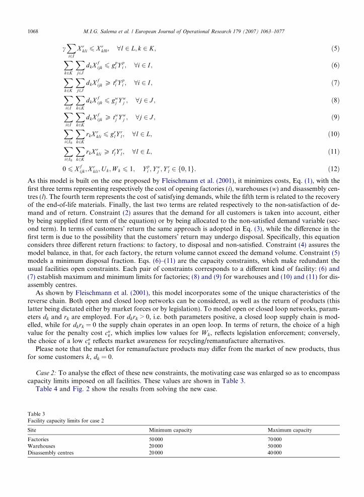
As this model is built on the one proposed by Fleischmann et al. (2001), it minimizes costs, Eq. (1), with thefirst three terms representing respectively the cost of opening factories (i), warehouses (w) and disassembly cen-tres (l). The fourth term represents the cost of satisfying demands, while the fifth term is related to the recoveryof the end-of-life materials. Finally, the last two terms are related respectively to the non-satisfaction of de-mand and of return. Constraint (2) assures that the demand for all customers is taken into account, eitherby being supplied (first term of the equation) or by being allocated to the non-satisfied demand variable (sec-ond term). In terms of customers’ return the same approach is adopted in Eq. (3), while the difference in thefirst term is due to the possibility that the customers’ return may undergo disposal. Specifically, this equationconsiders three different return fractions: to factory, to disposal and non-satisfied. Constraint (4) assures themodel balance, in that, for each factory, the return volume cannot exceed the demand volume. Constraint (5)models a minimum disposal fraction. Eqs. (6)–(11) are the capacity constraints, which make redundant theusual facilities open constraints. Each pair of constraints corresponds to a different kind of facility: (6) and(7) establish maximum and minimum limits for factories; (8) and (9) for warehouses and (10) and (11) for dis-assembly centres.
As shown by Fleischmann et al. (2001), this model incorporates some of the unique characteristics of thereverse chain. Both open and closed loop networks can be considered, as well as the return of products (thislatter being dictated either by market forces or by legislation). To model open or closed loop networks, param-eters dk and rk are employed. For dkrk > 0, i.e. both parameters positive, a closed loop supply chain is mod-elled, while for dkrk = 0 the supply chain operates in an open loop. In terms of return, the choice of a highvalue for the penalty cost cu
k , which implies low values for Wk, reflects legislation enforcement; conversely,the choice of a low cu
k reflects market awareness for recycling/remanufacture alternatives.Please note that the market for remanufacture products may differ from the market of new products, thus
for some customers k, dk = 0.
Case 2: To analyse the effect of these new constraints, the motivating case was enlarged so as to encompasscapacity limits imposed on all facilities. These values are shown in Table 3.
Table 4 and Fig. 2 show the results from solving the new case.
3y capacity limits for case 2
Minimum capacity Maximum capacity
ies 50000 70000ouses 20000 50000embly centres 20000 40000
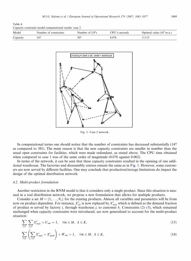
Table 4Capacity constraint model computational results: case 2
Model Number of constraints Number of LP’s CPU’s (second) Optimal value (103 m.u.)
Capacity 147 207 0.078 11115
Fig. 2. Case 2 network.
M.I.G. Salema et al. / European Journal of Operational Research 179 (2007) 1063–1077 1069
In computational terms one should notice that the number of constraints has decreased substantially (147as compared to 381). The main reason is that the new capacity constraints are smaller in number than theusual open constraints for facilities, which were made redundant, as stated above. The CPU time obtainedwhen compared to case 1 was of the same order of magnitude (0.078 against 0.062).
In terms of the network, it can be seen that these capacity constraints resulted in the opening of one addi-tional warehouse. The factories and disassembly centres remain the same as in Fig. 1. However, some custom-ers are now served by different facilities. One may conclude that production/storage limitations do impact thedesign of the optimal distribution network.
4.2. Multi-product formulation
Another restriction in the RNM model is that it considers only a single product. Since this situation is unu-sual in a real distribution network, we propose a new formulation that allows for multiple products.
Consider a set M = {1, . . . ,Nv} for the existing products. Almost all variables and parameters will be fromnow on product dependent. For instance, X f
ijk is now replaced by X fmijk which is defined as the demand fraction
of product m served by factory i, through warehouse j, to customer k. Constraints (2)–(5), which remainedunchanged when capacity constraints were introduced, are now generalized to account for the multi-productsituation:
Xi2I
Xj2J
X fmijk þ Umk ¼ 1; 8m 2 M ; k 2 K; ð13Þ
Xl2L
Xi2I
X rmkli þ X r
mkl0
!þ W mk ¼ 1; 8m 2 M ; k 2 K; ð14Þ
TableProdu
Descri
Transp
FactorWarehCostumDisassDemanReturnNot saNot sa
Model
cfijk ¼
whe
1070 M.I.G. Salema et al. / European Journal of Operational Research 179 (2007) 1063–1077
Xk2K
Xl2L
rmkX rmkli 6
Xj2J
Xk2K
dmkX fmijk; 8m 2 M ; i 2 I ; ð15Þ
cXi2I
X rmkli 6 X r
mkl0; 8m 2 M ; l 2 L; k 2 K. ð16Þ
Constraints (6)–(11), which impose limits to facility capacities, will be replaced by constraints that will limitthe total capacity of facilities. These limits refer to the total processing/warehousing of all products that runthrough the network.
As an example, the changes in factory capacity constraints are presented. Changes are similar for theremaining constraints. Constraints (6) and (7) are now rewritten as follows:
Xm2M
Xk2K
Xj2J
dmkX fmijk 6 gp
i Y pi ; 8i 2 I ; ð17Þ
Xm2M
Xk2K
Xj2J
dmkX fmijk P tp
i Y pi ; 8i 2 I . ð18Þ
Furthermore, we can easily account for the possibility of limiting the production of each product:
Xk2KXj2J
dmkX fmijk 6 gp
miYpi ; 8m 2 M ; i 2 I ; ð19Þ
Xk2K
Xj2J
dmkX fmijk P tp
miYpi ; 8m 2 M ; i 2 I ; ð20Þ
where gpmi and tp
mi are, respectively, the maximum and minimum production limits of product m for factory i.Case 3: Case 2 is now implemented for two products. Product one has the same data used in the previous
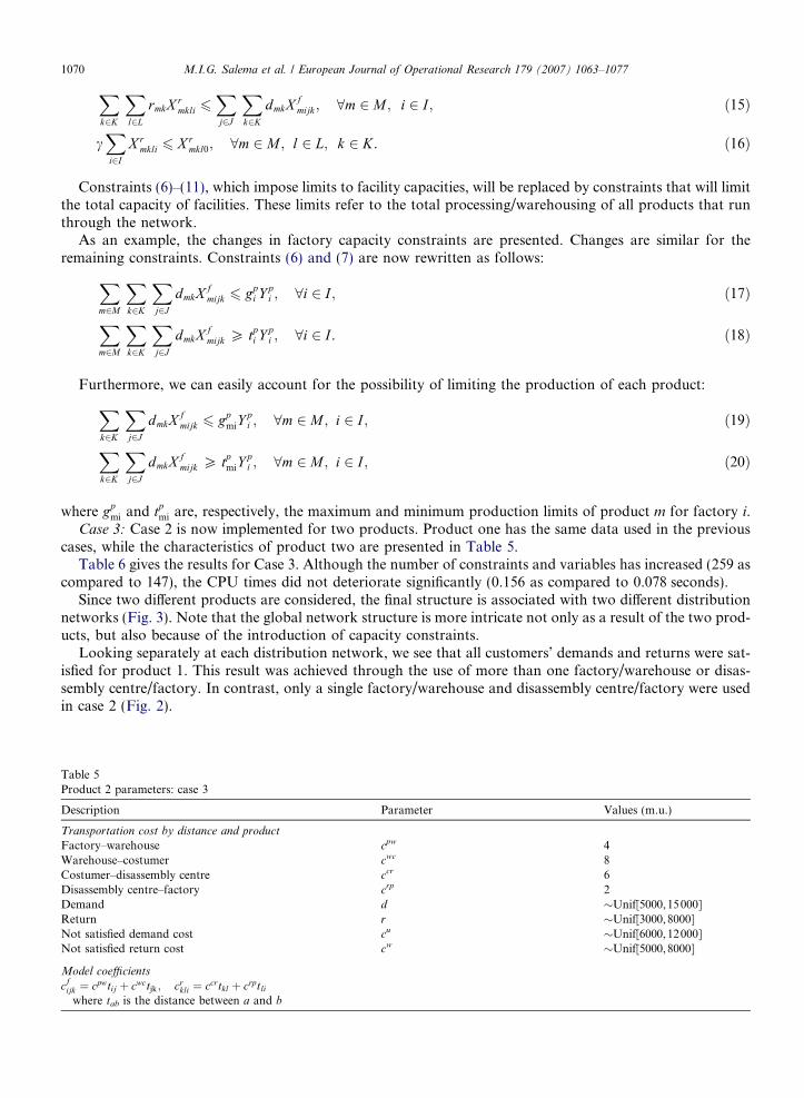
cases, while the characteristics of product two are presented in Table 5.Table 6 gives the results for Case 3. Although the number of constraints and variables has increased (259 as
compared to 147), the CPU times did not deteriorate significantly (0.156 as compared to 0.078 seconds).Since two different products are considered, the final structure is associated with two different distribution
networks (Fig. 3). Note that the global network structure is more intricate not only as a result of the two prod-ucts, but also because of the introduction of capacity constraints.
Looking separately at each distribution network, we see that all customers’ demands and returns were sat-isfied for product 1. This result was achieved through the use of more than one factory/warehouse or disas-sembly centre/factory. In contrast, only a single factory/warehouse and disassembly centre/factory were usedin case 2 (Fig. 2).
5ct 2 parameters: case 3
ption Parameter Values (m.u.)
ortation cost by distance and product
y–warehouse cpw 4ouse–costumer cwc 8er–disassembly centre ccr 6
embly centre–factory crp 2d d �Unif[5000,15000]
r �Unif[3000,8000]tisfied demand cost cu �Unif[6000,12000]tisfied return cost cw �Unif[5000,8000]
coefficients
cpwtij þ cwctjk; crkli ¼ ccrtkl þ crptli
re tab is the distance between a and b
Table 6Case 3 computational results
Model Total variables Binary variables Number of constraints Number of LP’s CPU’s (seconds) Optimal value (103 m.u.)
Multi 2179 18 259 444 0.156 20420
Fig. 3. Case 3 networks for product 1 and 2, respectively.
M.I.G. Salema et al. / European Journal of Operational Research 179 (2007) 1063–1077 1071
With regard to product 2, again all customers’ demands and returns were satisfied. In Fig. 3 it seems thatone disassembly centre was opened just to collect one customer’s return sent totally for disposal (because thereis no link between that centre and the factory located in Salamanca). However in the network for product 1,the same disassembly centre serves three more customers and sends the returned products to the factorylocated in Madrid.
It is important to note that the global structure is obtained for the two products and the distribution ismade simultaneously for both products.
4.3. Uncertainty
Literature shows that one of the major problems in the reverse logistic chains is the uncertainty associatedwith demand and return. Hence, this problem should be addressed when trying to model such systems. In thispaper we employ a scenario-based approach to model such conditions.
4.3.1. Uncertainty approach
Let H be the set of all possible scenarios and h 2 H a particular scenario. Also, let all binary variables beincluded in vector y and all the continuous variables in vector x. Let f be the vector of the fixed costs related tothe opening of the facilities and c the vector containing the remaining coefficients in the objective function.
For a particular scenario h, the concise model can be stated as follows:
min fy þ chx
Ahx 6 ah;
Bhx 6 Cy;
y 2 f0; 1g; x P 0;
where Ah, Bh and C are matrices and ah is a vector.
1072 M.I.G. Salema et al. / European Journal of Operational Research 179 (2007) 1063–1077
Consider ph to be the probability of scenario h. Since we only wish to model a finite number of discretescenarios, the expected value function becomes an ordinary sum. The uncertainty model is then given bythe following mixed integer formulation:
min fy þX
h
phchxh
Ahxh 6 ah;
Bhxh 6 Cy;
y 2 f0; 1g; xh P 0.
Note that the obtained solution for this model is not optimal for individual scenarios, but it gives the network struc-ture for the worst possible scenario. For further details, please refer to the work of Birge and Louveaux (1997).
4.3.2. Detailed modelAssuming that only customers’ demand and return are scenario-dependent, the remaining parameters have
the same values in the three scenarios. This includes the binary variables, which translate the condition ofwhether or not facilities are opened. As a consequence, only the continuous variables will vary with thescenario.
Based on the uncertainty approach described above, the capacitated multi-product reverse network modelcan be defined as follows:
Sets
In addition to the sets described in Section 4.1, we addM = {1, . . . ,Nv} existing products,S = {1, . . . ,Ns} potential scenarios.
Parameters
The same parameters defined in Section 4.1 will be employed. However some will require generalization forproduct m and scenario s, and a scenario probability needs to be added, as follows:dmks demand of product m, of customer k in the reuse market, for scenario s, m 2M, k 2 K, s 2 S,rmks return of used product m, of customer k, for scenario s, m 2M, k 2 K, s 2 S,cf
mijk unit variable cost of demand of product m, served by factory i, through warehouse j, to customer k
(may include transportation, production costs, . . .) m 2M, i 2 I, j 2 J, k 2 K,cr
mkli unit variable cost of product m return by customer k, through disassembly centre l, to factory i (mayinclude transportation costs, reprocessing costs, . . .), m 2M, k 2 K, l 2 L, i 2 I,
crmkl0 unit variable cost of product m disposal collected in customer k, through disassembly centre l, m 2M,
k 2 K, l 2 L,cu
mk unit variable cost for non-satisfied demand of product m for customer k, m 2M, k 2 K,cw
mk unit variable cost for non-satisfied return of product m, of customer k, m 2M, k 2 K,ps probability of scenario s, s 2 S.
Variables
Similar to parameters, some variables used in Section 4.1 will be modified, as follows:X f
mijks demand fraction of product m, served by factory i, through warehouse j, to customer k, in scenario s,m 2M, i 2 I, j 2 J, k 2 K, s 2 S – forward flow,
X rmklis return fraction of product m, made by customer k, through disassembly centre l, to factory i, in sce-
nario s, m 2M, k 2 K, l 2 L, i 2 I0, s 2 S – reverse flow,Umks non-satisfied demand fraction of product m, of customer k, in scenario s, m 2M, k 2 K, s 2 S,Wmks non-satisfied return fraction of product m of customer k, in scenario s, m 2M, k 2 K, s 2 S.
M.I.G. Salema et al. / European Journal of Operational Research 179 (2007) 1063–1077 1073
Formulation
MinXm2M
Xi2I
Xj2J
Xk2K
Xs2S
pscfmijkdmksX
fmijks þ
Xm2M
Xk2K
Xl2L
Xi2I0
Xs2S
pscrmklirmksX r
mklis
þXm2M
Xk2K
Xs2S
pscumkdmksU mks þ
Xm2M
Xk2K
Xs2S
pscwmkrmksW mks
þXi2I
f pi Y p
i þXj2J
f wj Y w
j þXl2L
f rl Y r
l ð21Þ
s.t.Xi2I
Xj2J
X fmijks þ Umks ¼ 1; 8m 2 M ; k 2 K; s 2 S ð22Þ
Xl2L
Xi2I
X rmklis þ X mkl0s
!þ W mks ¼ 1; 8m 2 M ; k 2 K; s 2 S ð23Þ
Xk2K
Xl2L
rmksX rmklis 6
Xj2J
Xk2K
dmksXfmijks; 8m 2 M ; i 2 I ; s 2 S ð24Þ
cXi2I
X rmklis 6 X r
mkl0; 8m 2 M ; l 2 L; k 2 K; s 2 S ð25ÞXm2M
Xk2K
Xj2J
dmksXfmijks 6 gp
i Y pi ; 8i 2 I ; s 2 S ð26Þ
Xm2M
Xk2K
Xj2J
dmksXfmijks P tp
i Y pi ; 8i 2 I ; s 2 S ð27Þ
Xm2M
Xi2I
Xk2K
dmksXfmijks 6 gw
j Y wj ; 8j 2 J ; s 2 S ð28Þ
Xm2M
Xi2I
Xk2K
dmksXfmijks P tw
j Y wj ; 8j 2 J ; s 2 S ð29Þ
Xm2M
Xi2I0
Xk2K
rmksX rmklis 6 gr
lYrl; 8l 2 L; s 2 S ð30Þ
Xm2M
Xi2I0
Xk2K
rmksX rmklis P tr
lYrl; 8l 2 L; s 2 S ð31Þ
0 6 X fmijks;X
rmklis;U mks;W mks 6 1; Y p
i ; Ywj ; Y
rl 2 f0; 1g. ð32Þ
This model not only maintains the characteristics of the model proposed by Fleischmann et al. (2001), where itis possible to model open or closed loop supply chains and demand push or pull drivers, but also allows themodelling of a multi-product network with capacity constraints.
Case 4: Since the previous networks were designed for new products, the data provided by the companywere based on estimated values. Consequently, a model accounting for some uncertainty in the provided datawas identified as a useful tool. A scenario-based model was then built, which can provide the decision makerswith an adequate framework to investigate different patterns of product demand and return.
Again as data are confidential, different values were generated to run case 4. So the previous two productswill again be considered, together with capacity constraints. Three scenarios for each product will beestablished.
The scenarios for demand and return are described in Table 7. The data from case 3 are preserved in sce-nario 1 for both products. Scenario 2 of product 1 models the most pessimistic situation and scenario 3 modelsan optimistic one. For product 2 similar economic situations are also modelled: scenario 2 is optimistic whilescenario 3 is pessimistic.
For each scenario there is an associated probability value (10%, 75% and 15%, respectively). The example issolved with CPLEX version 8.1 and the results are presented in Table 8 and Figs. 4 and 5.
Analysing the computational results, it can be seen that, as expected, the model size increased significantlyand the CPU time grew accordingly, together with the number of LP’s needed to solve the case instance.
Fig. 4 presents the various scenario networks created for product 1. It is found that all customers are servedand that 100% service, in both demand and return, is guaranteed. This is shown in Figs. 5–7.
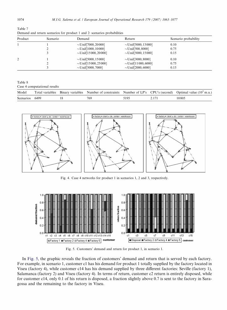
Table 7Demand and return scenarios for product 1 and 2: scenarios probabilities
Product Scenario Demand Return Scenario probability
1 1 �Unif[7000,20000] �Unif[5000,13000] 0.102 �Unif[1000,10000] �Unif[500,8000] 0.753 �Unif[15000,20000] �Unif[5000,15000] 0.15
2 1 �Unif[5000,15000] �Unif[3000,8000] 0.102 �Unif[15000,25000] �Unif[11000,6000] 0.753 �Unif[5000,7000] �Unif[2000,6000] 0.15
Table 8Case 4 computational results
Model Total variables Binary variables Number of constraints Number of LP’s CPU’s (second) Optimal value (103 m.u.)
Scenarios 6499 18 769 5195 2.171 10805
Fig. 4. Case 4 networks for product 1 in scenarios 1, 2 and 3, respectively.
Fig. 5. Customers’ demand and return for product 1, in scenario 1.
1074 M.I.G. Salema et al. / European Journal of Operational Research 179 (2007) 1063–1077
In Fig. 5, the graphic reveals the fraction of customers’ demand and return that is served by each factory.For example, in scenario 1, customer c1 has his demand for product 1 totally supplied by the factory located inViseu (factory 4), while customer c14 has his demand supplied by three different factories: Seville (factory 1),Salamanca (factory 2) and Viseu (factory 4). In terms of return, customer c2 return is entirely disposed, whilefor customer c14, only 0.1 of his return is disposed, a fraction slightly above 0.7 is sent to the factory in Sara-gossa and the remaining to the factory in Viseu.

M.I.G. Salema et al. / European Journal of Operational Research 179 (2007) 1063–1077 1075
It can be noted in Figs. 5–7, how customer c2 has his demand differently met in all three scenarios: in sce-nario 1 by the factories in Salamanca and Madrid (factory 5), in scenario 2 wholly by the Salamanca factory,and in scenario 3 wholly by the Madrid factory. The solution found for customer c15 is the opposite: supply isguaranteed by Madrid in all three scenarios. In terms of return, the solutions found for all the scenarios arenot very different. The same solution is found for all customers, exception made for customers c7, c8, c10 andc14, which have their return taken care by different factories.
Fig. 6. Customers’ demand and return for product 1, in scenario 2.
Fig. 7. Customers’ demand and return for product 1, in scenario 3.
Fig. 8. Case 4 networks for product 2 in scenarios 1 and 2, respectively.
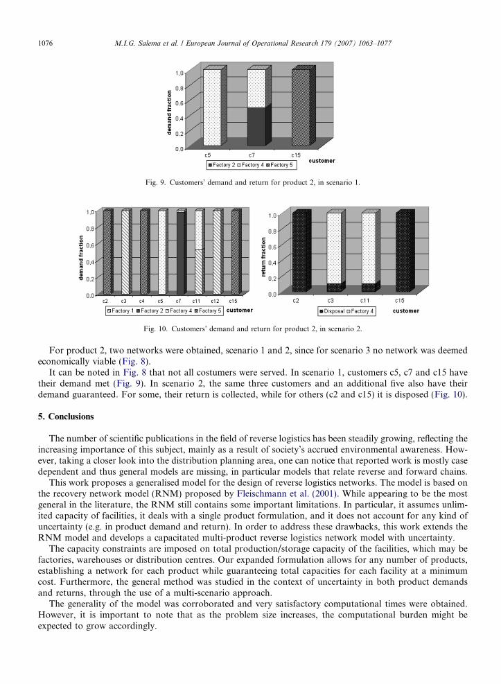
Fig. 9. Customers’ demand and return for product 2, in scenario 1.
Fig. 10. Customers’ demand and return for product 2, in scenario 2.
1076 M.I.G. Salema et al. / European Journal of Operational Research 179 (2007) 1063–1077
For product 2, two networks were obtained, scenario 1 and 2, since for scenario 3 no network was deemedeconomically viable (Fig. 8).
It can be noted in Fig. 8 that not all costumers were served. In scenario 1, customers c5, c7 and c15 havetheir demand met (Fig. 9). In scenario 2, the same three customers and an additional five also have theirdemand guaranteed. For some, their return is collected, while for others (c2 and c15) it is disposed (Fig. 10).
5. Conclusions
The number of scientific publications in the field of reverse logistics has been steadily growing, reflecting theincreasing importance of this subject, mainly as a result of society’s accrued environmental awareness. How-ever, taking a closer look into the distribution planning area, one can notice that reported work is mostly casedependent and thus general models are missing, in particular models that relate reverse and forward chains.
This work proposes a generalised model for the design of reverse logistics networks. The model is based onthe recovery network model (RNM) proposed by Fleischmann et al. (2001). While appearing to be the mostgeneral in the literature, the RNM still contains some important limitations. In particular, it assumes unlim-ited capacity of facilities, it deals with a single product formulation, and it does not account for any kind ofuncertainty (e.g. in product demand and return). In order to address these drawbacks, this work extends theRNM model and develops a capacitated multi-product reverse logistics network model with uncertainty.
The capacity constraints are imposed on total production/storage capacity of the facilities, which may befactories, warehouses or distribution centres. Our expanded formulation allows for any number of products,establishing a network for each product while guaranteeing total capacities for each facility at a minimumcost. Furthermore, the general method was studied in the context of uncertainty in both product demandsand returns, through the use of a multi-scenario approach.
The generality of the model was corroborated and very satisfactory computational times were obtained.However, it is important to note that as the problem size increases, the computational burden might beexpected to grow accordingly.
M.I.G. Salema et al. / European Journal of Operational Research 179 (2007) 1063–1077 1077
Due to this foreseen limitation, future work by the authors includes the application of decomposition meth-ods to the model. These methods can be generic as, for instance, benders decomposition, or methods that willexplore directly the problem structure.
References
Ammons, J. et al., 1997. Reverse production system design and operations for carpet recycling. Working paper, Georgia Institute ofTechnology, Atlanta, Georgia.
Barros, A.I. et al., 1998. A two-level network for recycling sand: A case study. European Journal of Operational Research 110, 199–214.Birge, J.R., Louveaux, F., 1997. Introduction to Stochastic Programming. Springer Series in Operations Research. Springer-Verlag, New
York.Caruso, C. et al., 1993. The regional urban solid waste management system: A modelling approach. European Journal of Operational
Research 70, 16–30.Fleischmann, M., 2001. Quantitative Models for Reverse Logistics. Lecture Notes in Economics and Mathematical Systems, vol. 501.
Springer-Verlag, Berlin.Fleischmann, M. et al., 2001. The impact of product recovery on logistics network design. Production and Operations Management 10,
156–173.Giannikos, I.A., 1998. Multiobjective programming model for locating treatment sites and routing hazardous wastes. European Journal of
Operational Research 104, 333–342.Gottinger, H.W., 1988. A computational model for solid waste management with application. European Journal of Operational Research
35, 350–364.Jayaraman, V. et al., 1999. A closed-loop logistics model for remanufacturing. Journal of Operational Research Society 50, 497–508.Krikke, H.R. et al., 2001. Design of closed-loop supply chains: A production and return network for refrigerators. Working paper ERS-
2001-45-LIS, Erasmus University Rotterdam, The Netherlands.Kroon, L., Vrijens, G., 1995. Returnable containers: An example of reverse logistics. International Journal of Physical Distribution and
Logistics 25, 56–68.Listes, O., Dekker, R., 2001. Stochastic approaches for product recovery network design: A case study. Working paper, Faculty of
Economics, Erasmus University Rotterdam, The Netherlands.Sodhi, M., Reimer, D., 2001. Models for recycling end-of-life products. OR-Sepktrum 23, 97–115.Spengler, T. et al., 1997. Environmental integrated production and recycling management. European Journal of Operational Research 97,
308–326.Stock, J.R., 1992. Reverse Logistics. Council of Logistics Management, Oak Brook, IL.Veerakamolmal, P., Gupta, S.M., 2000. Optimization the supply chain in reverse logistics. In: Proceedings of the SPIE International
Conference on Environmentally Conscious Manufacturing, vol. 4193, pp. 157–166.Voigt, K.I., 2001. Solutions for industrial reverse logistics systems. In: Proceedings of the Twelfth Annual Conference of Production and
Operations Management Society, POM 2001, Orlando, p. 4153.
Copyright © 2022 FDOKUMEN