An Investigation on the Aggregate Behavior of Firm Relocations to New Jersey (1990–1999) and the...

Networks and Spatial Economics, 5: (2005) 293–331©C 2005 Springer Science + Business Media, Inc. Manufactured in The Netherlands.

An Investigation on the Aggregate Behaviorof Firm Relocations to New Jersey (1990–1999)and the Underlying Market Elasticities

JOSE HOLGUIN-VERASDepartment of Civil and Environmental Engineering, Rensselaer Polytechnic Institute, 110 Eighth Street, 4030Jonsson Engineering Center, Troy, NY 12180email: [email protected]

NING XUDepartment of Civil and Environmental Engineering, Rensselaer Polytechnic Institute, 110 Eighth Street, 4037Jonsson Engineering Center, Troy, NY 12180email: [email protected]

HERBERT S. LEVINSONUniversity Transportation Research Center, Region 2, City College of New York, 138th Street and Convent Avenue,New York, NY 10031email: [email protected]

CLAIRE E. MCKNIGHTDepartment of Civil Engineering, City College of New York, 138th Street and Convent Avenue, New York, NY10031email: [email protected]

ROSS D. WEINERDepartment of Economics, City College of New York, 138th Street and Convent Avenue, New York, NY 10031email: [email protected]

ROBERT E. PAASWELLUniversity Transportation Research Center, Region 2, City College of New York, 138th Street and Convent Avenue,New York, NY 10031email: [email protected]

KAAN OZBAYDepartment of Civil and Environmental Engineering, Rutgers, The State University of New Jersey, 96 DavidsonRoad, Piscataway, NJ 08854email: [email protected]

DILRUBA OZMEN-ERTEKINUrbitran Associates, Inc., 623 Bowser Road, Piscataway, NJ 08854email: [email protected]

294 HOLGUIN-VERAS ET AL.

Abstract

This paper reports the key results of an in depth analysis of ten years worth of data about business relocations tothe State of New Jersey. The analyses have focused on the key geographic patterns of business relocations, andan econometric investigation of the role of transportation accessibility on the business relocation process. Theestimated models focus on explaining the business relocation behavior, as well as the business relocation flowsfrom the original locations to New Jersey.

The first model assumes that the probability of a business relocating to a given location in New Jersey is afunction of the combined attraction to the economic poles of New York City and Philadelphia. The results obtainedsuggest the existence of two opposing trends concerning the role played by New York City. The discrete choicemodels estimated provide additional insights into the role of transportation accessibility, suggesting that the typeof economic activity performed by the firm shapes the firm’s valuation of accessibility to markets.

The paper also studied the role of transportation accessibility as an explanatory variable of the business relocationflows by means of estimating aggregate demand models and destination constrained gravity models. In all casesthe authors were able to estimate statistically significant and conceptually valid models that explain the aggregatebehavior of the variables under study. These models were estimated for both the total number of relocations (allfirms) as well as the major industry types. The resulting models were used to compute the elasticities with respectto accessibility variables. The chief conclusion is that different industry types exhibit different elasticities.

In order to do the computations for the elasticities of the gravity model, the authors developed a mathematicalformulation. Simply stated, this formulation demonstrates that the elasticity of the spatial interaction between anorigin i and a destination j is simply the summation of the elasticities at the production end, and at the destination.The market elasticity is then computed as the weighted average of the elasticities for each of the market segments.

Keywords: business location, transportation accessibility, econometric modeling

Introduction

It is widely accepted that transportation accessibility is a necessary, though not sufficient,condition for economic development. In this context, the transportation system is consid-ered to enable economic interactions to take place across urban and regional geographies.This idea has found its way to the transportation planning process and, as a result, a keyobjective of transportation policy is to provide the conditions, in terms of transportationaccessibility, that makes economic development possible. To ensure efficient transportationinvestment, transportation planners and policy makers are interested in finding out the eco-nomic development impacts attributable to transportation investment and policy decisions,which ultimately enter as an input to formal, or informal, project evaluation processes.

Although economic development could take place in many different ways, this paperfocuses on a specific mechanism: business relocations (from the outside) to a given studyarea. The paper analyzes ten years of business relocation to the State of New Jersey, takingadvantage of a data set assembled and maintained by the New Jersey Department of Com-merce and Economic Growth that contains the information that companies moving intoNew Jersey provide when registering with the State.

This data set, once augmented with transportation accessibility variables, makes it possi-ble to develop a picture of the revealed linkages between business relocation and accessibilityindicators. The data have some limitations that arise because they do not contain informa-tion about: (a) companies moving out of New Jersey; (b) local taxes and/or tax incentivesprovided to the companies at the moment of relocation; and, (c) the actual choice set ofalternatives being considered by the companies. The main focus is on the analyses of the

INVESTIGATION ON THE AGGREGATE BEHAVIOR OF FIRM RELOCATIONS 295

relationship between business location patterns and transportation accessibility, which isaccomplished by estimating aggregate and disaggregate econometric models.

The paper is comprised of four major sections. The first one provides a succinct literaturereview on the subject of business location theory. The second section conducts a descriptiveanalysis of the business relocation patterns in New Jersey during the period 1990–1999. Thethird and fourth sections analyze, using econometric models, the relationship between busi-ness relocation decisions and accessibility, and business relocation flows and accessibility,respectively. The final section provides a summary of the key findings and conclusions.

Literature review

This section provides a succinct summary of the literature on business location modelingand theory. Due to the extent of the literature on the subject, the review focuses on the mostrelevant work to the purposes of the paper.

The work of Weber (1929) is considered to be the starting point of the analytical studyof industrial location. Weber states that the cost of transportation, labor, and rent are thekey variables explaining business location decisions. In its classic form, the fundamentalassumption of the Weber’s formulation is that individual firms choose the location thatminimizes the cost of production at the optimal production level, and the transportationcosts of input materials and finished products to markets. In this context, transportationcosts influence the assembly of inputs and the distribution of outputs and levels of demand,which are a key focus of industrial location theory.

Since Weber’s seminal contribution, there has been considerable discussion about the roleof transportation accessibility to input materials and markets in business location decisions.Two major schools of thought have emerged. The traditional point of view, following theWeber tradition, argues that industrial location decisions are a function of cost minimizationdecisions. An alternative perspective suggests that business location is a highly nuancedprocess, in which the decision makers take into account a host of different factors in additionto transportation accessibility. Some of the relevant literature is reviewed next.

Campbell (1958) concludes—on the basis of a survey of manufacturing firms which hadmoved out of New York City during the period 1947–1955— that space and site consid-erations dominate, yet taxes play a special role in the businessman’s locational decisionmaking, because they offer a clue to the political environment indicating its responsivenessor hostility to the demands of business.

Nishioka and Krumme (1973) define two relevant concepts of interest: location condi-tions and location factors. Location conditions are differences among locations that exist forall industries, while location factors refer to the specific importance that is attached to suchdifferences by individual firms when choosing locations for specific factories. Hayter (1997)suggests the following location conditions: transportation, materials, markets, labor, exter-nal economies (urbanization and localization), energy, community infrastructure, capital,land/buildings, environment, and government policy. While, location factors express howfirms assess places, location conditions have different implications for individual firms con-templating investment in new facilities. Firms interpret, or translate, location conditions aslocation factors which reflect their specific requirements for specific investment decisions.


Blackley and Greytak (1986) analyze the urban Heckscher-Ohlin (H-O) Effect, whichindicates that firms will seek location within the urban area in a manner determined by theirtechnologies, and their potential to substitute agglomeration economies and access for inter-nal capital. They estimate multinomial logit models for attribute demand in the Cincinnatimanufacturing market. Their results suggest two general conclusions. First, intrametropoli-tan access is becoming a relatively unimportant consideration for the manufacturing locationdecision. Second, spatial requirements related to the use of modern production process arestill a primary location factor.

Schneider (1985) states that firms have a wide range of preferences for local public goods.Some firms prefer higher service levels, while others prefer lower service levels. However,taxes are theoretically a more stringent constraint on the decisions of firms because theyrepresent costs that a business must face that may affect competitiveness.

Ponting and Waters (1985) indicate that market factors (e.g., proximity to markets, marketsize, centrality between markets, nature and amount of competition) emerge as the singlemost commonly cited important factor in influencing locational decisions. After that, themost important factor cited was the availability or proximity of inputs, including labor,energy, or other materials and supplies.

Harding (1986) states the criteria for selecting sites for headquarter and administrativeoffices. For headquarter offices, the location must be evaluated in terms of how it helps orhinders a company in achieving its corporate objectives. Also, management is likely to focuson travel time to such outside business associates as lawyers, accountants, advertisers, andothers. Meanwhile, a firm’s headquarters must often relocate when it outgrows its space,when there is a major reorganization within the firm, or when the firm merges with anothercompany. For administrative offices, minimizing costs is the key to choosing a location.

Giuliano (1989) states that relocation costs are a significant factor in any location-choicedecision. Given these costs, the expected benefits of a new location must be at least as great asthe cost of moving before relocation will take place. Her research, on firms that had relocatedfrom Milwaukee, Wisconsin, to suburbs between 1964 and 1974, shows that agglomerationeconomies and labor-force availability are the most significant factors explaining locationchoices for all industries. Firms may treat transportation accessibility as a constraint: someminimum must be fulfilled, but additional levels of accessibility have little value.

Chapman and Walker (1991) argue the role of transportation cost in industrial location.They describe two tendencies that have been important in affecting the relationship betweentransport cost and industrial cost in the twentieth century. The first concerns the way inwhich freight costs on the finished products have risen more rapidly than those on rawmaterials. Thus firms are willing to move near to their markets rather than their source ofraw material. The tendency is to ship raw materials further, perhaps to the market area, andcut down shipments of finished products. The second trend has been an overall decline inthe significance of transport costs as a proportion of total costs in most industries. Thereare a significant number of companies producing finished, higher-value goods better ableto bear the costs of transport.

Townroe (1991) indicates that elements of risk and uncertainty in business locationdecisions are typically high, including uncertainty about the most appropriate decision-making procedure. A “push” factor has to be involved as well as a set of “pull” factors


related to the new location. These push factors may involve cost elements (e.g., wages,access costs, the value of the land and property in alternative use, property taxes) or directconstraints, such as lack of adjacent space to expand into, land use planning controls,pollution controls, and end of lease.

Vickerman (1995) states that although improved accessibility does confer some potentialadvantages (in spite of having differential impacts across industries), it is the total impact oftransport that is critical. Karvel et al. (1998) analyze the business migration in Minnesota,and it indicates that the two most important reasons for business location decisions are: (1)workers’ compensation rates; and (2) commercial-industrial real estate tax rates. Locationof customers, transportation costs, and location of major supplies are all significantly lessimportant than the other reasons evaluated by respondents.

Leitham et al. (2000) suggest that it is important to disaggregate different types of re-locating firms when analyzing the importance of transport upon their location decisions.It is also important to distinguish between intra- and inter-regional moves. The study alsosuggests that stated preference techniques add useful additional insights, that are likely tocomplement analyses made with revealed preference data, in understanding the impact oftransport infrastructure and other factors upon location choice.

Kawamura (2001) studies the locations and profiles of firms in the six-county Chicagoregion for 1981 and 1999. The regression results indicate that, when controlling for exoge-nous factors such as agglomeration effects, factor prices, decentralization, and the densityof transportation facilities, businesses have moved closer to freeway ramps in the last twodecades, while the change of proximity to transit stations is not significant. The overallimportance of transportation access has not diminished. Rather, that firms in the urban coreareas value access to rail stations to a greater degree, while those in the suburbs placemore importance on proximity to freeway ramps. Thus, the findings indicate a shift in theimportance of transportation access for business location choice.

As shown in this succinct review, although accessibility is widely acknowledged to be alocation factor, there is no consensus about the specific role it has in the business locationchoice process. Equally lacking is research that explicitly considers the role of the type ofeconomic activity performed by the firm on the business location process.

The research documented in this paper tries to fulfill this void by: (a) analyzing the aggre-gate patterns of business decisions to New Jersey and their relationships to transportationaccessibility; and (b) estimating disaggregate business location choice models with explicitconsideration of the interactions between the type of firm and the accessibility variables.

Geographic patterns of business relocations to New Jersey

New Jersey is a densely settled state (see figure 1(a)). While the state is roughly rectangularwith the long axis oriented North-South, the locations of New York City to the northeastand Philadelphia about three quarters of the way down the west side of the state gives adiagonal axis to both development and the main transportation corridor (which connectsNew Jersey to the rest of the East Coast). The northeast part of the state (facing New YorkCity) is the most industrialized part of the state, with four old cities (Newark, Elizabeth,Jersey City, and Paterson) acting as centers to dense development. Development has spread


Figure 1. New Jersey counties and highway system (a) Counties and (b) Major highways.

out from this core, radiating along the transportation corridor (consisting of US 1, I-95,the New Jersey Turnpike, and the northeast passenger rail lines) connecting the northeastindustrial core to Trenton (the state capital) and Philadelphia (see figure 1(b)). A second,much smaller and less dense area of development radiates from Philadelphia. The northwestpart of the state is mountainous and has relatively little development. The southern part ofthe state is flat, but also largely undeveloped.

The transportation system in New Jersey includes marine ports and the Newark Interna-tional Airport, both in the northeast section of the state and both major stimulants to the NewJersey economy. Several major highways radiate from New York and the industrial corearound Newark, including the New Jersey Turnpike and US 1, the Garden State Parkway,which runs down the coast, and two Interstates (I-80 and I-78) that cross the northern partof the study area in an east-west direction. A circumferential interstate segment (I-287)circles the urbanized area around Newark and along the Hudson about 20 miles west ofthe Hudson. The northeast part of the state is served by an extensive commuter rail systemradiating from Newark and Hoboken and serving New York City. Additionally Amtrak’smain line (the Northeast Corridor) runs through New Jersey along the same corridor as theNew Jersey Transit main line from Newark to Trenton.

Economic activity and growth in New Jersey is strong. One factor that makes New Jerseystand out from other states is its role within U.S. freight network. The Commodity FlowSurvey (USDOT and USDOC, 1997) indicates that 223.9 million tons were transported


in New Jersey in 1997, translating into 34.45 billion ton-miles. Trucking is the dominantmode, with 84.9% of the total. For the most part, the cargoes are transported relatively shortdistances (72.5% are transported less than 50 miles, and 81.8% of the tons are transportedless than 100 miles). The Port of New York and New Jersey, largely located in New Jersey,is the largest East Coast port, making New Jersey a major transshipment location andmaking warehousing, transportation, and similar industries major contributors to the NewJersey economy. A second characteristic of the New Jersey economy is the large number ofpharmaceutical firms. While manufacturing in general grew slowly in New Jersey throughthe 1990s (7% over ten years), chemical manufacturing, which represents the largest groupwithin New Jersey manufacturing, grew 36%.

Description of data

The data analyzed were provided by the New Jersey Department of Commerce and Eco-nomic Growth, and they contain the information that companies moving into New Jerseyprovide when registering with the State. The data represent 1017 firms that relocated intoNew Jersey from outside the state or the country from 1990 through 1999. Intrastate movesor firms leaving the state are not included. Additionally, neither the reason that a firm de-cided to relocate nor whether the move represents an opening of a branch or a completemove is included.

The 1017 firms employed an estimated total of 108,000 employees and represent 74industries as represented by different NAICS (North American Industrial ClassificationSystem) codes. The original data set included the name of the firm, the year of registra-tion, the destination county and address in New Jersey, the state or country of origin, thenumber of employees, the (two digits) Standard Industrial Codes (SIC), and descriptionof the “line of business”. A substantial number of firms were missing addresses, numberof employees, and/or SIC codes. The missing codes were determined from the “line ofbusiness” description. For firms missing information for number of employees, the averagenumber of employees for firms with the same NAICS code was used. Research assistantsfound the addresses for those which were missing from the Internet or telephone books.Since the project team decided to use NAICS—because it provides a better description ofthe service sectors—a computer program was used to convert SIC two-digit codes, and theline of business descriptions, to NAICS three-digit codes.

Origins of firms

The origins of the firms appear to depend on some combination of proximity, size andtype of economic activity of the origin. Eighty eight percent (897 firms) originated withinthe United States (see Table 1); 54 percent (548 firms) came from New York State. Whennumber of employees (instead of number of firms) is used, New York State contributed62,625 employees over the ten years or 58 percent of the total. A large number of the firmscame from New York City, although the actual number cannot be precisely determined (thedata set was inconsistent, listing the origin as a city in some cases and a state in others).New York City is both immediately adjacent and the place of greatest economic activity.


Table 1. Origins of relocated firms and jobs (1990–1999).

Firms Jobs Jobs/firm

Origin (no.) (%) (no.) (%) Average

New York State 548 54 62625 58 114

Pennsylvania 99 10 10379 10 105

California 39 4 3978 4 102

Massachusetts 20 2 2314 2 116

Connecticut 18 2 1312 1 73

Illinois 16 2 1458 1 91

Georgia 14 1 2285 2 163

Texas 14 1 1103 1 79

Maryland 13 1 929 1 71

Virginia 13 1 1367 1 105

Florida 13 1 1231 1 95

Ohio 11 1 747 1 68

Delaware 10 1 777 1 78

Colorado 8 1 452 0 57

Washington 6 1 1418 1 236

Minnesota 5 0 524 0 105

Arkansas 5 0 119 0 24

Michigan 4 0 354 0 89

Missouri 3 0 826 1 275

North Carolina 3 0 801 1 267

Other States (18) 35 3 2776 3 79

Total United States 897 88 97775 91 109

Canada 17 2 1134 1 67

United Kingdom 19 2 1726 2 91

Germany 17 2 1547 1 91

Switzerland 5 0 231 0 46

Other countries (9) 16 2 1265 1 79

Total Europe 57 6 4769 4 84

Japan 16 2 1930 2 121

Korea 8 1 641 1 80

Other countries (4) 4 0 52 0 13

Total Pacific Rim 28 3 2623 2 94

Other & unknown (4) 18 2 1714 2 95

All foreign countries 120 12 10240 9 85

Grand Total 1017 100 108015 100 106


The next most frequent origin (99 firms) is Pennsylvania. Philadelphia is also immediatelyadjacent to New Jersey and a location of sizable economic activity. However, the third mostfrequent origin is California (39 firms), at the opposite end of the country.

Eleven percent, or 120 firms, originated from outside the United States from 22 differentcountries; 57 firms came from Europe, with the United Kingdom (19 firms) the singlelargest foreign origin. After the United Kingdom, the top foreign origins were Canada(17), Germany (17), and Japan (16). Twenty eight firms came from Pacific Rim countries,including Japan. Not surprisingly the countries of origin are dominated by strong economies.Using number of employees as the measure of contribution, Japan moves to the top of theforeign origins, with 1930 employees, or two percent of the total.

The size of the relocated firms tends to shrink slightly with distance from New Jersey.Firms moving from New York State have an average of 114 employees; from the rest of theUnited States, an average of 109 employees; and those from outside the country have an av-erage of 85 employees. However, the 16 firms from Japan had an average of 121 employees.

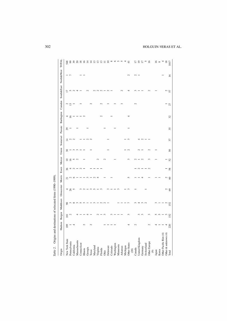
Table 2 shows the counties where the firms located within New Jersey by origin. (Thecounties and origins are in rank order of number of firms. Counties that received fewerthan 20 firms were grouped into two larger zones: North & West counties and South & Eastcounties.) As can be seen, the largest flow (189 firms) was from New York to Hudson County.Hudson County faces midtown and lower Manhattan (where the largest concentration ofjobs are) across the Hudson River and has direct connection to Manhattan via the PATHtrain (a commuter subway), the Lincoln and Hudson Tunnels (which handle cars and manyexpress buses), and ferry service.

The next largest flow (101 firms) is from New York to Bergen County, across the Hudsonfrom the northern part of Manhattan and connected by the George Washington Bridge.The third largest (90 firms) is from New York to Middlesex County; Middlesex is slightlyfurther from New York City, but has been growing rapidly over the last several decades.The next three largest flows of firms are from New York to three counties (Essex, Union,and Passaic) in the northeastern industrial core of New Jersey, all counties with substantialexisting economic bases. The largest flow from an origin other than New York is 26 firmsthat relocated from Pennsylvania to Gloucester County, which is immediately to the southof Philadelphia, across the Delaware River.

When the flow of jobs, rather than firms, is considered (see Table 3), the move fromNew York to Hudson County still leads, with 24,178 jobs representing 22% of the totalflow of jobs into New Jersey (compared to 19% of the actual number of firms). The percentof Pennsylvania firms that move to Gloucester County (26%) is the same as the percentof jobs, but the remaining Pennsylvania jobs are more concentrated than the firms, withMercer County receiving 22%, and Camden and Burlington each receiving 12% of thejobs. Gloucester, Camden, and Burlington form the New Jersey suburban counties forPhiladelphia. Georgia, Missouri, Texas, and Washington show up in Table 3 because of oneor a couple of large firms.

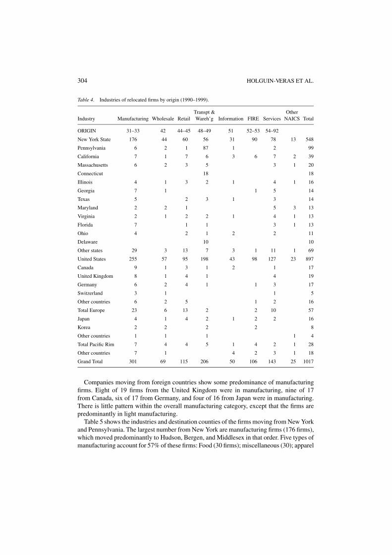
The predominant industry of the relocating firms (see Table 4) is manufacturing, whichaccounts for 301 firms (29%). By type of manufacturing, the leading firms are: miscel-laneous (53), food manufacturing (42), chemical manufacturing, which includes pharma-ceutical companies (32), and computer and electronic products (28). After manufacturing,


Tabl

e2.

Ori

gins

and

dest

inat

ions

ofre

loca

ted

firm

s(1

990–

1999

).

Ori

gin

Hud

son

Ber

gen

Mid

dles

exG

louc

este

rM

orri

sE

ssex

Mer

cer

Uni

onSo

mer

set

Pass

aic

Bur

lingt

onC

amde

nSo

uth&

Eas

tN

orth

&W

est

TO

TAL

New

Yor

kSt

ate

189

101

904

2136

1030

1429

42

171

548

Penn

sylv

ania

12

326

24

161

21

1613

57

99C

alif

orni

a4

85

62

53

21

12

39M

assa

chus

etts

43

11

23

11

420

Con

nect

icut

15

31

21

11

11

118

Illin

ois

21

32

11

11

12

116

Geo

rgia

41

13

21

214

Texa

s2

11

31

11

22

14M

aryl

and

35

21

213

Vir

gini

a2

11

41

22

13Fl

orid

a1

23

12

22

13O

hio

13

21

21

111

Del

awar

e1

13

11

12

10C

olor

ado

13

11

11

8W

ashi

ngto

n1

11

11

16

Min

neso

ta1

13

5A

rkan

sas

11

12

5M

ichi

gan

11

11

4O

ther

Stat

es4

37

35

32

31

44

241

(20)

Can

ada

23

11

12

23

217

Uni

ted

Kin

gdom

34

12

12

41

119

Ger

man

y3

34

12

12

117

Switz

erla

nd2

11

15

Oth

erE

urop

e2

31

23

21

216

(9)

Japa

n4

53

11

11

16K

orea

15

11

8O

ther

Paci

ficR

im(4

)1

11

14

Oth

er&

unkn

own

(4)

43

22

21

11

218

Tota

l22

015

215

269

6058

5250

3735

3227

5716

1017


Table 3. Major flows of jobs (1990–1999).

COUNTY NY PA CA GA WA TX MO Japan UK Total

Hudson 24178 500 610 26876

Bergen 12449 603 16627

Middlesex 9824 573 15040

Morris 3649 599 1020 7769

Gloucester 803 2713 677 7175

Mercer 763 2318 1041 6494

Somerset 2315 501 768 5082

Essex 2552 514 4909

Union 2206 3672

Burlington 504 1259 2914

Camden 1263 525 2740

Passaic 1834 2268

Monmouth 694 1622

Total 62625 10379 3978 2285 1418 1103 826 1930 1726 108015

Note: Only flows of 500 and more are shown.

the highly represented industries are: transportation and warehousing (206), service in-dustries (143), retail (115), and finance, insurance, and real estate (FIRE—106). In theservice category, 57 firms (40% of the 143 firms) are in professional, scientific, andtechnical services, and another 25 (17%) are in administrative and support services. Thepattern of industries for only those firms that originated in the United States is similar.Interestingly, all firms that moved from Connecticut and Delaware were in transportationand warehousing.

The types of industries represented by the firms relocating from New York also showa similar pattern in that the largest category is manufacturing (176 out of the 548 firms).However, the FIRE category is second with 90 firms, service follows with 78 firms, retailfollows with 60 firms, transportation and warehousing follows with 56 firms; and wholesaletrade is sixth with 44 firms. Within manufacturing, the two largest categories are food (30)and miscellaneous (30); chemical manufacturing is third with 15 firms. The movement oftransportation and warehousing (and also wholesale trade) from New York to New Jerseyfollows a long term trend. Given the high cost of land, congestion within New York City,and the more direct connection to the rest of the country from New Jersey, the large freightindustry associated with the New York/New Jersey Port has tended to migrate from the NewYork to the New Jersey side of the Hudson River.

Firms relocating from Pennsylvania are dominated by transportation and warehousing(87 of the 99 firms). For California, the third largest origin, manufacturing with sevenfirms, particularly computer and electronic products manufacturing (4), and professional,scientific, and technical services (5 firms) are the largest categories. Professional servicesis an area that has shown high growth in New Jersey over the last decade and also onepredicted for strong growth in the next several years.


Table 4. Industries of relocated firms by origin (1990–1999).

Transpt & OtherIndustry Manufacturing Wholesale Retail Wareh’g Information FIRE Services NAICS Total

ORIGIN 31–33 42 44–45 48–49 51 52–53 54–92

New York State 176 44 60 56 31 90 78 13 548

Pennsylvania 6 2 1 87 1 2 99

California 7 1 7 6 3 6 7 2 39

Massachusetts 6 2 3 5 3 1 20

Connecticut 18 18

Illinois 4 1 3 2 1 4 1 16

Georgia 7 1 1 5 14

Texas 5 2 3 1 3 14

Maryland 2 2 1 5 3 13

Virginia 2 1 2 2 1 4 1 13

Florida 7 1 1 3 1 13

Ohio 4 2 1 2 2 11

Delaware 10 10

Other states 29 3 13 7 3 1 11 1 69

United States 255 57 95 198 43 98 127 23 897

Canada 9 1 3 1 2 1 17

United Kingdom 8 1 4 1 4 19

Germany 6 2 4 1 1 3 17

Switzerland 3 1 1 5

Other countries 6 2 5 1 2 16

Total Europe 23 6 13 2 2 10 57

Japan 4 1 4 2 1 2 2 16

Korea 2 2 2 2 8

Other countries 1 1 1 1 4

Total Pacific Rim 7 4 4 5 1 4 2 1 28

Other countries 7 1 4 2 3 1 18

Grand Total 301 69 115 206 50 106 143 25 1017

Companies moving from foreign countries show some predominance of manufacturingfirms. Eight of 19 firms from the United Kingdom were in manufacturing, nine of 17from Canada, six of 17 from Germany, and four of 16 from Japan were in manufacturing.There is little pattern within the overall manufacturing category, except that the firms arepredominantly in light manufacturing.

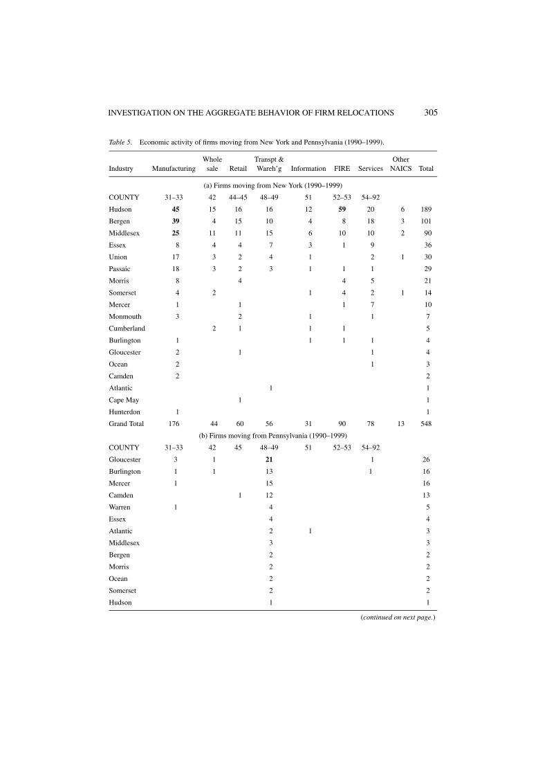
Table 5 shows the industries and destination counties of the firms moving from New Yorkand Pennsylvania. The largest number from New York are manufacturing firms (176 firms),which moved predominantly to Hudson, Bergen, and Middlesex in that order. Five types ofmanufacturing account for 57% of these firms: Food (30 firms); miscellaneous (30); apparel


Table 5. Economic activity of firms moving from New York and Pennsylvania (1990–1999).

Whole Transpt & OtherIndustry Manufacturing sale Retail Wareh’g Information FIRE Services NAICS Total

(a) Firms moving from New York (1990–1999)

COUNTY 31–33 42 44–45 48–49 51 52–53 54–92

Hudson 45 15 16 16 12 59 20 6 189

Bergen 39 4 15 10 4 8 18 3 101

Middlesex 25 11 11 15 6 10 10 2 90

Essex 8 4 4 7 3 1 9 36

Union 17 3 2 4 1 2 1 30

Passaic 18 3 2 3 1 1 1 29

Morris 8 4 4 5 21

Somerset 4 2 1 4 2 1 14

Mercer 1 1 1 7 10

Monmouth 3 2 1 1 7

Cumberland 2 1 1 1 5

Burlington 1 1 1 1 4

Gloucester 2 1 1 4

Ocean 2 1 3

Camden 2 2

Atlantic 1 1

Cape May 1 1

Hunterdon 1 1

Grand Total 176 44 60 56 31 90 78 13 548

(b) Firms moving from Pennsylvania (1990–1999)

COUNTY 31–33 42 45 48–49 51 52–53 54–92

Gloucester 3 1 21 1 26

Burlington 1 1 13 1 16

Mercer 1 15 16

Camden 1 12 13

Warren 1 4 5

Essex 4 4

Atlantic 2 1 3

Middlesex 3 3

Bergen 2 2

Morris 2 2

Ocean 2 2

Somerset 2 2

Hudson 1 1

(continued on next page.)


Table 5. (continued).

Manu- Whole Retail Transpt & Infor- OtherIndustry facturing sale Wareh’g mation FIRE Services NAICS Total

Hunterdon 1 1

Passaic 1 1

Sussex 1 1

Union 1 1

Grand Total 6 2 1 87 1 2 99

(15); chemical (15); and computer and electronic products (11). The next largest categoryis finance, insurance, and real estate (FIRE—90 firms). Thirty-nine (39) of these were insecurity intermediation and related activities. Two thirds of these located to Hudson County.This is expected; anecdotal evidence for years has indicated that many of the Wall Streetfirms have been moving their back office operations across the river to Hudson County, NewJersey, and Hudson County has courted these firms with lower taxes and other incentives.

Firms in various service industries were the third largest group, with professional, scien-tific, and technical services (NAICS 541) the largest subgroup with 32 firms. The servicefirms from New York tended to locate in a pattern similar to firms overall, with the greatestnumber in Hudson, Bergen, and Middlesex. Retail firms (60) are the next dominant industrywith transportation and warehousing following with 56 firms. Thirty-three of these latterwere warehouses or storage facilities.

Looking at the flows from Pennsylvania, 87 of the 99 firms were in transportation andwarehousing, and 21 of these relocated to Gloucester County, which is the location of amajor rail terminal. We suspect that many of these are moving from Philadelphia eitherto be nearer the rail terminal or to find cheaper available land. Interestingly firms in thetransportation and warehousing category moved from Pennsylvania to 17 of the 21 NewJersey counties.

Destinations of firms

Table 6 shows the counties to which the firms moved (in rank order of number of firms),along with the number of jobs and average employment per firm. Over half of the firms(524 firms) relocated to just three of New Jersey’s twenty-one counties: Bergen, Hudson,and Middlesex. Nine of the top ten counties were located in the northern New Jersey, withthe top three counties for business relocation located across from New York City. Together,these nine counties accounted for 80 percent of all business relocations in the study.

The majority of firms fall into five groups: Manufacturing (NAICS 31, 32, and 33),Transportation and warehousing (48–49), Services (54 through 92), Retail trade (44–45),and Finance, insurance and real estate or FIRE (52-53). Table 7a provides information onthe number of firms by industrial group and year they moved. The greatest number of firmsmoved at the beginning and end of the 1990s, reaching a peak in 1999 with 118 companies


Table 6. Destinations of relocated firms and jobs in New Jersey (1990–1999).

Firms Employment Jobs/firm

County no. (%) no. (%) Average

Hudson 220 21.6 26876 24.9 122

Bergen 152 14.9 16627 15.4 109

Middlesex 152 14.9 15040 13.9 99

Gloucester 69 6.8 7175 6.6 104

Morris 60 5.9 7769 7.2 129

Essex 58 5.7 4909 4.5 85

Mercer 52 5.1 6494 6.0 125

Union 50 4.9 3672 3.4 73

Somerset 37 3.6 5082 4.7 137

Passaic 35 3.4 2268 2.1 65

Burlington 32 3.1 2914 2.7 91

Camden 27 2.7 2740 2.5 101

Cumberland 16 1.6 910 0.8 57

Monmouth 15 1.5 1622 1.5 108

Ocean 10 1.0 785 0.7 79

Warren 10 1.0 683 0.6 68

Atlantic 8 0.8 744 0.7 93

Cape May 4 0.4 445 0.4 111

Hunterdon 4 0.4 524 0.5 131

Salem 4 0.4 440 0.4 110

Sussex 2 0.2 296 0.3 148

Total 1017 100.0 108015 100.0 106

relocating to New Jersey. There was a general increase in the number of relocations to NewJersey from 1990 to 1999. On average, 101 firms moved to New Jersey per year, with astandard deviation of 11.8.

The percentages of firms in the major industrial groups were stable across the decade.Firms in manufacturing were the largest group, for every year in the study. Transportationand warehousing constituted 20 percent of the total moves and were the second largestcategory in all but one year. Observing these groups over time, no distinct temporal patternwithin any particular group is apparent. However, when viewed as a whole, the numberof firms moving to New Jersey within these groupings trends generally upward, especiallyafter 1993.

Table 7b provides the number of jobs and jobs associated with firms relocating to NewJersey by year and industrial group. Manufacturing provides both the largest number of firmsand of jobs, and is close to average in company size with 100 employees per company. Thelargest firms are in the FIRE industries, with an average of 170 employees per firm. The


Table 7. Firms and jobs relocated by year and industry (1990–1999).

Whole Transpt & OtherManufacturing sale Retail wareh’g Information FIRE Services NAICS Total

(a) Firms relocated by year and industry (1990–1999)FIRMSYear 31–33 42 44–45 48–49 51 52–53 54–92

1990 26 5 13 26 5 4 16 3 98

1991 33 5 4 22 3 15 20 3 105

1992 32 4 14 25 6 12 13 3 109

1993 25 7 4 15 4 8 12 3 78

1994 33 7 10 16 3 9 12 6 96

1995 27 9 16 18 17 10 1 98

1996 23 7 17 13 6 8 19 2 95

1997 38 9 8 17 9 8 15 1 105

1998 38 9 11 28 5 9 13 2 115

1999 26 7 18 26 9 18 13 1 118

Total 301 69 115 206 50 108 143 25 1017

(b) Jobs relocated by year and industry (1990–1999).JOBSYear 31–33 42 44–45 48–49 51 52–53 54–92

1990 2949 203 715 3325 890 582 1281 86 10031

1991 4055 208 236 1737 261 3454 2603 314 12868

1992 2854 254 1532 1716 526 2327 1382 75 10666

1993 2825 594 604 1255 499 2236 1161 2 9176

1994 2524 433 1021 1296 194 1730 1940 79 9217

1995 2590 734 1390 1122 2090 940 2 8868

1996 1595 261 1202 1115 582 691 1535 54 7035

1997 4101 176 1441 3658 2145 1278 3386 2 16187

1998 4221 542 714 2010 416 1180 1442 215 10740

1999 2456 390 2421 2436 1055 2763 1706 13227

Total jobs 30170 3795 11276 19670 6568 18331 17376 829 108015

Total firms 301 69 115 206 50 108 143 25 1017

Jobs/firm 100 55 98 95 131 170 122 33 106

next largest firms are in information (e.g., broadcasting and telecommunications) with 131employees per firm and services, with 122 employees per firm. Over the decade, the totalnumber of jobs associated with relocating firms falls from 1991 to 1996, after which itjumps rather markedly. Breaking this trend down by sector reveals that a large part of thistrend comes from transportation and warehousing, FIRE, and manufacturing.

While there does not appear to be a temporal trend in the movement of the industries,a geographic pattern can be seen (see Table 8). Sixty-eight of the 108 FIRE firms (63%)


Table 8. Relocated firms by industries and counties (1990–1999).

Transpt & Whole OtherIndustry Manufacturing wareh’g Services Retail FIRE sale Information NAICS Total

County 31–33 48–49 54–92 44–45 52–53 42 51

Hudson 48 22 23 21 68 16 16 6 220

Bergen 54 19 26 24 11 8 7 3 152

Middlesex 45 30 20 19 10 16 10 2 152

Gloucester 17 32 6 7 3 4 69

Morris 18 4 14 12 5 3 2 2 60

Essex 12 14 12 10 2 4 4 58

Mercer 8 18 15 3 2 4 1 1 52

Union 25 8 4 3 2 4 2 2 50

Somerset 11 6 6 4 4 4 1 1 37

Passaic 21 4 2 3 1 3 1 35

Burlington 6 16 5 1 2 1 1 32

Camden 7 14 3 1 1 1 27

Cumberland 7 2 2 1 1 2 1 16

Monmouth 7 1 3 2 2 15

Ocean 4 2 1 1 1 1 10

Warren 4 5 1 10

Atlantic 2 4 1 1 8

Cape May 2 1 1 4

Hunterdon 2 1 1 4

Salem 2 1 1 4

Sussex 1 1 2

Total 301 206 143 115 108 69 50 25 1017

moving to New Jersey moved into Hudson County. Twenty-six of the 143 service firms(including 15 of the 57 professional service firms) moved to Bergen County, along with 19transportation and warehousing firms. This may be due to the large employment base ofBergen County, along with its proximity to New York and various transportation systems.A rather large number of transportation and warehousing firms (30) relocated to the Mid-dlesex County. Thirteen professional service firms also relocated there, along with eightfirms in chemical manufacturing, out of 45 total manufacturing firms. The large number oftransportation and warehousing firms may be due to Middlesex County’s location on thenortheast rail corridor, the presence of several major highways, including the Garden StateParkway, the New Jersey Turnpike, and Route 1. The large number of professional servicefirms may reflect the presence of Rutgers University and the county’s proximity to PrincetonUniversity. Many of the firms in chemical manufacturing may be pharmaceuticals, whichenjoy a strong presence throughout New Jersey.


The remaining counties in New Jersey have no distinct patterns, with the notable exceptionof transportation and warehousing in Gloucester County, with 32 firms, and in MercerCounty, with 18 firms. The large presence of such businesses in these counties may have todo with proximity to Philadelphia and the associated rail corridor.

Transportation accessibility and business relocation decisions

The main objective of this section is to use econometric models to help analyze the role oftransportation accessibility in the business relocation. A significant number of the modelsare aggregate in nature because they focus on depicting the behavior of clusters of specificindustry segments. Several different models are discussed. The first model is an aggregatebusiness location model that is based on the assumption that the business location decisionstake into account the combined attraction produced by the economic poles of Philadelphiaand New York City. The second set of models focus on depicting the business relocationflows to New Jersey. This paper also discusses basic results from disaggregate modeling ofthe business relocation choice process that, in spite of some limitations provide additionalinsights.

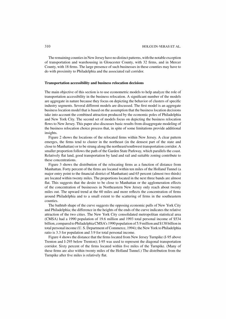
Figure 2 shows the locations of the relocated firms within New Jersey. A clear patternemerges, the firms tend to cluster in the northeast (in the densest part of the state andclose to Manhattan) or to be strung along the northeast/southwest transportation corridor. Asmaller proportion follows the path of the Garden State Parkway, which parallels the coast.Relatively flat land, good transportation by land and rail and suitable zoning contribute tothese concentrations.

Figure 3 shows the distribution of the relocating firms as a function of distance fromManhattan. Forty percent of the firms are located within ten miles of the Holland Tunnel (amajor entry point to the financial district of Manhattan) and 65 percent (almost two thirds)are located within twenty miles. The proportions located in the next three bands are almostflat. This suggests that the desire to be close to Manhattan or the agglomeration effectsof the concentration of businesses in Northeastern New Jersey only reach about twentymiles out. The upward trend at the 60 miles and more reflects the concentration of firmsaround Philadelphia and to a small extent to the scattering of firms in the southeasterncounties.

The bathtub shape of the curve suggests the opposing economic pulls of New York Cityand Philadelphia; the difference in the heights of the ends of the curve indicates the relativeattraction of the two cities. The New York City consolidated metropolitan statistical area(CMSA) had a 1990 population of 19.6 million and 1993 total personal income of $534billion, compared to Philadelphia CMSA’s 1990 population of 5.9 million and $138 billion intotal personal income (U. S. Department of Commerce, 1994); the New York to Philadelphiaratio is 3.3 for population and 3.9 for total personal income.

Figure 4 shows the distance that the firms located from New Jersey Turnpike (I-95 aboveTrenton and I-295 below Trenton); I-95 was used to represent the diagonal transportationcorridor. Sixty percent of the firms located within five miles of the Turnpike. (Many ofthese firms are also within twenty miles of the Holland Tunnel.) The distribution from theTurnpike after five miles is relatively flat.


Figure 2. Business relocation to New Jersey (1990–1999).

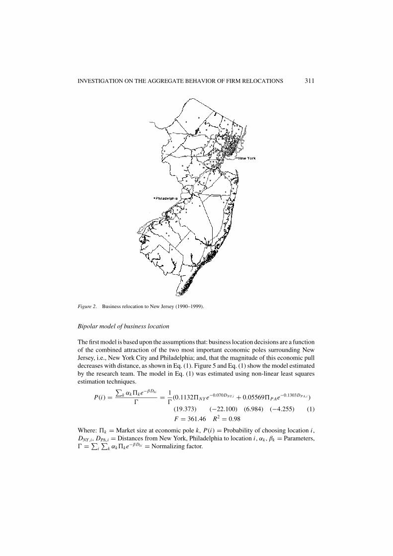
Bipolar model of business location

The first model is based upon the assumptions that: business location decisions are a functionof the combined attraction of the two most important economic poles surrounding NewJersey, i.e., New York City and Philadelphia; and, that the magnitude of this economic pulldecreases with distance, as shown in Eq. (1). Figure 5 and Eq. (1) show the model estimatedby the research team. The model in Eq. (1) was estimated using non-linear least squaresestimation techniques.

P(i) =∑

k αk�ke−β Dki

�= 1

�(0.1132�NY e−0.070DNY,i + 0.05569�P Ae−0.1303DP A,i )

(19.373) (−22.100) (6.984) (−4.255) (1)

F = 361.46 R2 = 0.98

Where: �k = Market size at economic pole k, P(i) = Probability of choosing location i ,DNY,i, DPA,i = Distances from New York, Philadelphia to location i , αk, βk = Parameters,� = ∑

i

∑k αk�ke−β Dki = Normalizing factor.


Figure 3. Distance of firms from New York.

Figure 4. Distance of relocated firms from NJ Turnpike.


Figure 5. Actual and estimated values of business location model.

As shown in Eq. (1), the absolute value of the parameter β for New York City (−0.07)is almost half the value of the one corresponding to Philadelphia (−0.1303). Since thisparameter is an indication of the weight assigned to the travel distance to the economicpoles, it signals that—in equality of conditions—firms would tend to locate farther awayfrom New York City. This is likely to reflect numerous factors not captured by this simplemodel, including: high levels of congestion and land costs in the surroundings of New YorkCity, among other things. On the other hand, the coefficient α, for New York City (0.1132)which measures the relative importance of population (a proxy of market size) is almosttwice the value of the one corresponding to Philadelphia (0.05569). In other words, one unitof population in New York City is twice as attractive as a unit of population in Philadelphia.This may be a reflection of perceived economies of densities and the higher per capitaincome in New York City.

In essence, Eq. (1) suggests the existence of two opposing effects. Businesses seem tobe attracted to the high density of the New York City market and its economic potential.At the same time, they are deterred by high congestion and real estate costs. The observedpatterns of relocation suggest that the former effect still dominates because the bulk ofthe relocations to New Jersey are congregated suburban areas close to New York and toa lesser extent to Philadelphia. While many of the firms, particularly those moving fromNew York, were seeking less expensive land, lower taxes, the importance of access still hasa major influence on their locational decisions. The concentration of new firms in alreadydense areas has significant implications for the transportation system of both passengersand freight and would add significant stresses to a transportation system that is alreadyoverloaded.

In terms of elasticity, as the reader could verify, Eq. (1) has variable elasticity equalto: η = −β Di (Di is the distance to either New York City or Philadelphia, and β is the


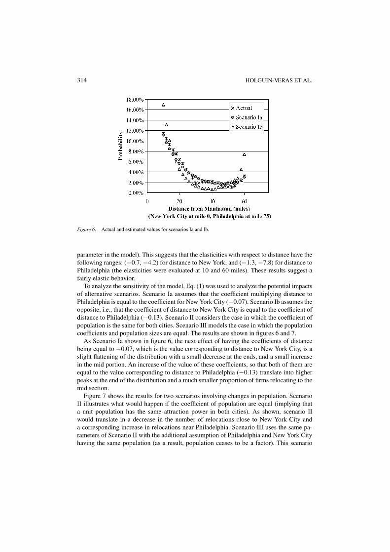
Figure 6. Actual and estimated values for scenarios Ia and Ib.

parameter in the model). This suggests that the elasticities with respect to distance have thefollowing ranges: (−0.7, −4.2) for distance to New York, and (−1.3, −7.8) for distance toPhiladelphia (the elasticities were evaluated at 10 and 60 miles). These results suggest afairly elastic behavior.

To analyze the sensitivity of the model, Eq. (1) was used to analyze the potential impactsof alternative scenarios. Scenario Ia assumes that the coefficient multiplying distance toPhiladelphia is equal to the coefficient for New York City (−0.07). Scenario Ib assumes theopposite, i.e., that the coefficient of distance to New York City is equal to the coefficient ofdistance to Philadelphia (−0.13). Scenario II considers the case in which the coefficient ofpopulation is the same for both cities. Scenario III models the case in which the populationcoefficients and population sizes are equal. The results are shown in figures 6 and 7.

As Scenario Ia shown in figure 6, the next effect of having the coefficients of distancebeing equal to −0.07, which is the value corresponding to distance to New York City, is aslight flattening of the distribution with a small decrease at the ends, and a small increasein the mid portion. An increase of the value of these coefficients, so that both of them areequal to the value corresponding to distance to Philadelphia (−0.13) translate into higherpeaks at the end of the distribution and a much smaller proportion of firms relocating to themid section.

Figure 7 shows the results for two scenarios involving changes in population. ScenarioII illustrates what would happen if the coefficient of population are equal (implying thata unit population has the same attraction power in both cities). As shown, scenario IIwould translate in a decrease in the number of relocations close to New York City anda corresponding increase in relocations near Philadelphia. Scenario III uses the same pa-rameters of Scenario II with the additional assumption of Philadelphia and New York Cityhaving the same population (as a result, population ceases to be a factor). This scenario


Figure 7. Actual and estimated values for scenarios II and III.

would translate into majority of the relocations going to the Philadelphia area, instead ofNew York City.

Disaggregate models of business location

Before discussing the models in this section, it is important to highlight that, since thedatabase only contained information about companies that decided to relocate to NewJersey, the disaggregate models estimated cannot be used to make general conclusionsabout business location choice behavior. In essence, these are conditional choice modelsthat represent the choice of location, given that the decision makers decided to relocate toNew Jersey. In spite of this limitation, as shall be seen, the models do provide additionalinsights about the role of the economic activity performed by the firm and the correspondingvaluation of accessibility.

The first step in the disaggregate analyses was to create a Geographic Information Systems(GIS) containing the firms’ new location, the general information provided when registeringin New Jersey, and the zonal socio-economic attributes (e.g., population, population density,area, median income) extracted from the population census. The GIS was used to performspatial analyses and to define a zoning system. The main objective of the zoning systemwas to reduce the size of the choice set considered for modeling purposes so that, insteadof modeling a system of same complexity as real life process, the analysis could focus onmodeling the choice of a zone (as opposed to individual pieces of property). The zoningsystem attempted to define internally “homogenous” zones, in terms of key socio-economiccharacteristics such as income. Three different zoning systems were created (with 8, 25, and63 zones). The first two zoning systems covered the study area (Northern New Jersey), whilethe third one covered the entire state of New Jersey. The 25 zones system is shown in figure 8.


Figure 8. Twenty five zone zoning system.

The original database was complemented with two different sets of transportation acces-sibility measures. The fist one captures the travel impedances from each zone to the majorpopulation centers of New York City and Philadelphia, using the travel times as a proxy.The second set of accessibility measures captured the travel impedance to destinations inNew Jersey by means of the accessibility index suggested by Allen et al. (1993), whichwas generated for (a) highway and (b) transit modes. All of the accessibility variables wereestimated using the travel time data from the New Jersey Department of Transportationtravel demand model. The resulting database was then used for model estimation, afterconverting it to the appropriate format.

The models used here are modified versions of the traditional multinomial logit model(MNL) (see Ben-Akiva and Lerman, 2000). This modification is intended to ensure that theMNL be able to properly represent a spatial choice among a set of zones, as opposed toindividual pieces of property. This modification is necessary because, in real life, decisionmakers choose where to locate business among a set of specific properties or tracts of land,which constitutes the elemental alternatives (which could range in the thousands, and evenmillions). Modeling this decision process at this level of detail is a huge challenge becauseit requires collecting data about the elemental alternatives considered in the choice set, andthe estimation of a huge number of utility functions (though this could be ameliorated byusing sampling of alternatives estimation techniques).

Fortunately, it can be shown that under rather general assumptions discrete choice modelscould be used to model the choice process for aggregations of elemental alternatives (zones).


In its most general formulation (see Ben-Akiva and Lerman, 2000), the decision to choosean alternative i among a set of aggregated alternatives, can be represented by a modifiedMultinomial Logit of the form shown in Eq. (2).

Pn(i) = eµ∗Vin+µ′ ln(Mi )+µ′ ln(Bin )∑Jj eµ∗Vjn+µ′ ln(M j )+µ′ ln(B jn )

(2)

Where:

Mi =K∑

k=K ′+1

βk xink or alternatively Mi =K∑

k=K ′+1

xinkeβk (3)

Bin = 1

Mi

∑l∈Li

eµ(Vln−Vin ) (4)

Mi is a measure of the size of alternative i , xink are the variables measuring the size ofaggregate alternative i (e.g., area, population, total employment), while Bin captures the vari-ability of the utilities of the elemental alternatives contained in aggregate alternative i . Theparameter µ′ = µ∗/µ is the ratio of the corresponding scale parameters, which are inverselyrelated to the variance of the error terms, because the error terms for the aggregated alter-natives are larger than the ones corresponding to the elemental alternatives, it follows that:

0 ≤ µ′ ≤ 1 (5)

Since the estimation of the general model of Eq. (2) requires: (a) specialized software notavailable to the project team; and (b) data about the variability measure Bin (which were notavailable either), the project team decided to use a simplified form of Eq. (2). The simplifiedmodel is built under two assumptions. The first one is that the variability measure Bin isapproximately equal among aggregate alternatives and, for that reason, can be taken out ofthe model. The second assumption is that the measure of size Mi , could be appropriatelycaptured by a single variable. Under these assumptions, Eq. (6) is obtained:

Pn(i) = eµ∗Vin+µ′ ln(Mi )∑Jj eµ∗Vjn+µ′ ln(M j )

= eµ∗Vin+µ′ ln(xink)+µ′βk∑Jj eµ∗Vjn+µ′ ln(xjnk)+µ′βk

(6)

As shown in Eq. (6), using a single variable to represent Mi translates into a modelformulation that is similar to MNL and that, as a result, can be estimated using the statisticalpackages available to the project team. In general terms, the models considered a basic set ofzonal attributes (e.g., median income, population), accessibility variables (e.g., travel timesto New York and Philadelphia, highway and transit accessibility indexes) and interactionterms between the accessibility variables and the binary variables representing the differentNAICS.

The two best models are shown in Tables 9 and 10. The only difference between themis that Model 1 considers the average crime rate per year, while Model 2 includes theaverage land price and median income. As shown, the models share common features, mostnotably: relatively low goodness of fit, that transportation accessibility to New York Cityand Philadelphia is a factor, and that different types of business place different valuationsto accessibility. In both models, the coefficients of the size variable are statistically equal to


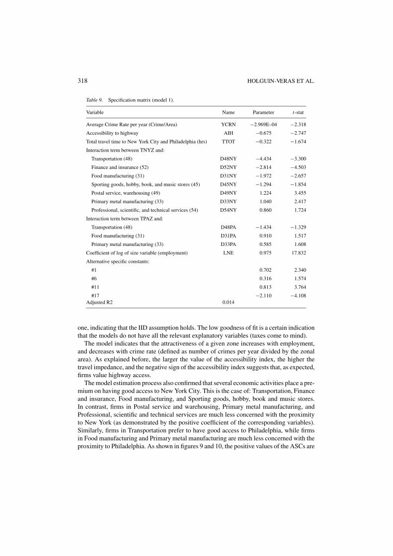
Table 9. Specification matrix (model 1).

Variable Name Parameter t-stat

Average Crime Rate per year (Crime/Area) YCRN −2.969E–04 −2.318

Accessibility to highway AIH −0.675 −2.747

Total travel time to New York City and Philadelphia (hrs) TTOT −0.322 −1.674

Interaction term between TNYZ and:

Transportation (48) D48NY −4.434 −3.300

Finance and insurance (52) D52NY −2.814 −4.503

Food manufacturing (31) D31NY −1.972 −2.657

Sporting goods, hobby, book, and music stores (45) D45NY −1.294 −1.854

Postal service, warehousing (49) D49NY 1.224 3.455

Primary metal manufacturing (33) D33NY 1.040 2.417

Professional, scientific, and technical services (54) D54NY 0.860 1.724

Interaction term between TPAZ and:

Transportation (48) D48PA −1.434 −1.329

Food manufacturing (31) D31PA 0.910 1.517

Primary metal manufacturing (33) D33PA 0.585 1.608

Coefficient of log of size variable (employment) LNE 0.975 17.832

Alternative specific constants:

#1 0.702 2.340

#6 0.316 1.574

#11 0.813 3.764

#17 −2.110 −4.108Adjusted R2 0.014

one, indicating that the IID assumption holds. The low goodness of fit is a certain indicationthat the models do not have all the relevant explanatory variables (taxes come to mind).

The model indicates that the attractiveness of a given zone increases with employment,and decreases with crime rate (defined as number of crimes per year divided by the zonalarea). As explained before, the larger the value of the accessibility index, the higher thetravel impedance, and the negative sign of the accessibility index suggests that, as expected,firms value highway access.

The model estimation process also confirmed that several economic activities place a pre-mium on having good access to New York City. This is the case of: Transportation, Financeand insurance, Food manufacturing, and Sporting goods, hobby, book and music stores.In contrast, firms in Postal service and warehousing, Primary metal manufacturing, andProfessional, scientific and technical services are much less concerned with the proximityto New York (as demonstrated by the positive coefficient of the corresponding variables).Similarly, firms in Transportation prefer to have good access to Philadelphia, while firmsin Food manufacturing and Primary metal manufacturing are much less concerned with theproximity to Philadelphia. As shown in figures 9 and 10, the positive values of the ASCs are


Table 10. Specification matrix (model 2).

Variable Name Parameter t-stat

Average land price (Land price/Area) YLPN −1.678E–09 −2.892

Median income INCN −8.092E-06 −1.755

Accessibility to highway AIH −0.603 −2.191

Total travel time to New York City and Philadelphia (hrs) TTOT −0.328 −1.740

Interaction term between TNYZ and:

Transportation (48) D48NY −4.156 −3.206

Finance and insurance (52) D52NY −2.681 −4.373

Food manufacturing (31) D31NY −1.873 −2.578

Sporting goods, hobby, book, and music stores (45) D45NY −1.223 −1.781

Postal service, warehousing (49) D49NY 1.217 3.483

Primary metal manufacturing (33) D33NY 1.012 2.404

Professional, scientific, and technical services (54) D54NY 0.863 1.756

Interaction term between TPAZ and:

Transportation (48) D48PA −1.265 −1.193

Food manufacturing (31) D31PA 0.976 1.637

Primary metal manufacturing (33) D33PA 0.557 1.526

Coefficient of log of size variable (employment) LNE 1.027 14.945

Alternative specific constants:

#1 0.701 2.346

#6 0.376 1.832

#11 0.872 4.002

#17 −2.048 −3.948

Adjusted R2 0.0154

along the northeast part of the state and the major transportation corridors, which indicatesinnate preference to relocation to these areas.

Among the zonal attributes, it was found that median income, crime rate and averageland price all have negative relationship with the likelihood of business relocation to thearea. The higher their values are, the less likely business will relocate to the area. From theconceptual point of view, these results make sense.

Transportation accessibility and business relocation flows

This section explores the role of transportation accessibility as an explanatory variable of thebusiness relocation flows between their original locations and the New Jersey destinations.Two basic sets of models were estimated. The first set consisted of aggregate demandfunctions, while the second set was comprised of destination constrained gravity models.


Figure 9. Values of the alternative specific constants (ASCs).

Figure 10. Values of the alternative specific constants (ASCs).

Aggregate demand functions

These models attempt to capture the relationship between the number of firms and employeesrelocating to New Jersey as the dependent variables, and airline distance, travel time, outof pocket expenses, and generalized travel costs as proxies for the cost of relocation. Theprimary assumption is that the underlying dynamics can be captured in the form of an


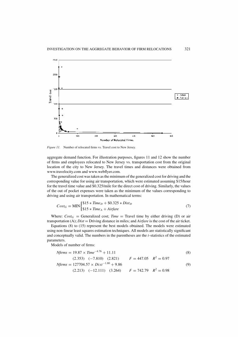
Figure 11. Number of relocated firms vs. Travel cost to New Jersey.

aggregate demand function. For illustration purposes, figures 11 and 12 show the numberof firms and employees relocated to New Jersey vs. transportation cost from the originallocation of the city to New Jersey. The travel times and distances were obtained fromwww.travelocity.com and www.webflyer.com.

The generalized cost was taken as the minimum of the generalized cost for driving and thecorresponding value for using air transportation, which were estimated assuming $15/hourfor the travel time value and $0.325/mile for the direct cost of driving. Similarly, the valuesof the out of pocket expenses were taken as the minimum of the values corresponding todriving and using air transportation. In mathematical terms:

CostG = MIN

{$15 ∗ TimeD + $0.325 ∗ DistD

$15 ∗ TimeA + Airfare(7)

Where: CostG = Generalized cost; Time = Travel time by either driving (D) or airtransportation (A); Dist = Driving distance in miles; and Airfare is the cost of the air ticket.

Equations (8) to (15) represent the best models obtained. The models were estimatedusing non-linear least squares estimation techniques. All models are statistically significantand conceptually valid. The numbers in the parentheses are the t-statistics of the estimatedparameters.

Models of number of firms:

Nfirms = 19.87 × Time−4.76 + 11.11 (8)

(2.353) (−7.810) (2.821) F = 447.05 R2 = 0.97

Nfirms = 127704.57 × Dist−1.80 + 9.86 (9)

(2.213) (−12.111) (3.264) F = 742.79 R2 = 0.98


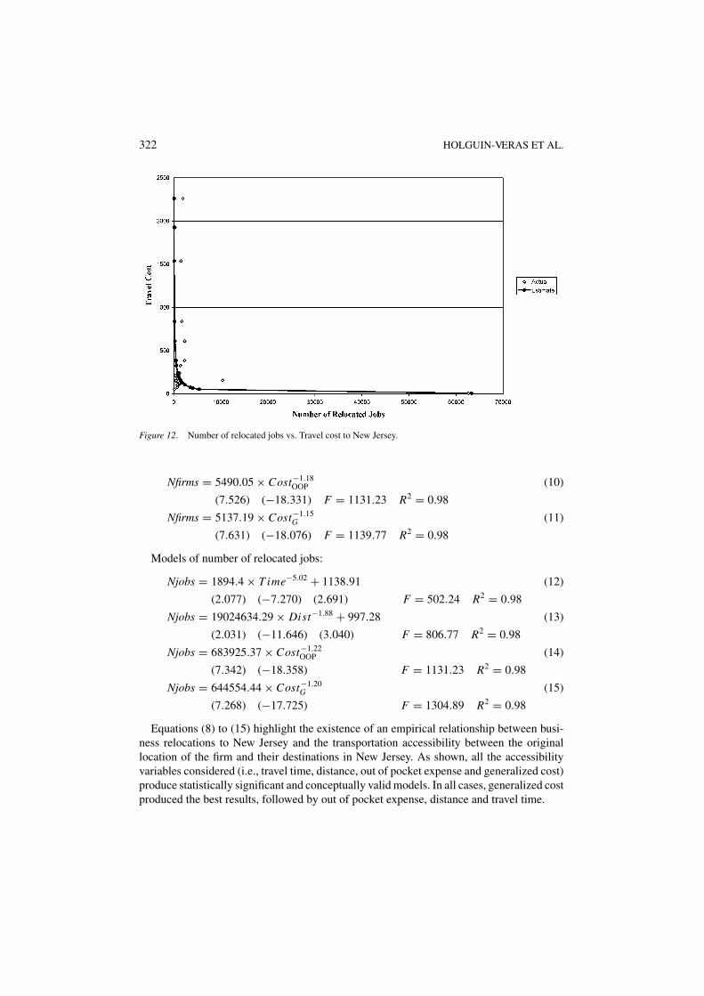
Figure 12. Number of relocated jobs vs. Travel cost to New Jersey.

Nfirms = 5490.05 × Cost−1.18OOP (10)

(7.526) (−18.331) F = 1131.23 R2 = 0.98

Nfirms = 5137.19 × Cost−1.15G (11)

(7.631) (−18.076) F = 1139.77 R2 = 0.98

Models of number of relocated jobs:

Njobs = 1894.4 × T ime−5.02 + 1138.91 (12)

(2.077) (−7.270) (2.691) F = 502.24 R2 = 0.98

Njobs = 19024634.29 × Dist−1.88 + 997.28 (13)

(2.031) (−11.646) (3.040) F = 806.77 R2 = 0.98

Njobs = 683925.37 × Cost−1.22OOP (14)

(7.342) (−18.358) F = 1131.23 R2 = 0.98

Njobs = 644554.44 × Cost−1.20G (15)

(7.268) (−17.725) F = 1304.89 R2 = 0.98

Equations (8) to (15) highlight the existence of an empirical relationship between busi-ness relocations to New Jersey and the transportation accessibility between the originallocation of the firm and their destinations in New Jersey. As shown, all the accessibilityvariables considered (i.e., travel time, distance, out of pocket expense and generalized cost)produce statistically significant and conceptually valid models. In all cases, generalized costproduced the best results, followed by out of pocket expense, distance and travel time.


Table 11. Elasticities for different models.

Accessiblility variables

Elasticity Time Distance Min cost Gen cost

Firms −4.76 −1.80 −1.18 −1.15

Jobs −5.02 −1.88 −1.22 −1.20

Table 12. Estimates of parameters of aggregate demand function by industry type.

Industry NAICS Alpha Beta R-sq (%) Number of firms Number of data points

Manufacturing 31–33 2403.94 1.3410 99.5 226 11

Wholesale 42 545.45 1.2912 99.8 54 8

Retail 44–45 732.86 1.2842 97.8 82 10

Information 51 341.14 1.2307 98.3 40 7

Services 54–92 683.80 1.1149 98.2 116 11

Other NAICS 49.91 0.6895 97.7 22 7

Transportation and 48-49 171.88 0.5084 38.4 191 11warehousing

All Firms 5137.19 1.1472 98.0 862 20

Note: The model for finance, insurance, and real estate (FIRE) could not be estimated because the number of datapoints for calibration was too small.

The models provide different results in terms of the elasticities derived (see Table 11). Inthe models based on travel time and distance, the elasticities are higher than 1.8 in absolutevalue, indicating highly elastic demand. The models based on costs have smaller elasticitiescloser to the absolute value of one (unit elasticity).

Table 12 shows the results of the aggregate demand models by industry type, using themodel Nfirms = α×Cost−β

G . As shown in Table 12, most industry segments have elasticitiesin the vicinity of 1.00, which corresponds to unit elasticity.

Destination constrained gravity models

One limitation of the aggregate demand functions is that they do not take into accountthe impact of the size of the market at the origin of the business relocation flow, which isexpected to be an explanatory variable. In this context, the larger the size of the economyat the origin, the larger the business relocation flows it sends to other areas. Among otherthings, the lack of explicit consideration of this variable may translate into a misspecificationerror and, ultimately, erroneous conclusions about the role of transportation accessibility.To overcome this limitation, a destination constrained gravity model (single constraint) wasused. This decision was taken because the gravity model enables explicit consideration of


Table 13. Estimates of parameters of gravity model by industry type.

Sum of Number of Number ofIndustry NAICS Beta squared errors R-sq (%) firms data points

Wholesale 42 0.0345 0.0124 98.3 54 8

Information 51 0.0320 0.0291 95.9 40 7

Manufacturing 31–33 0.0300 0.0188 97.2 226 11

Retail 44–45 0.0253 0.0351 93.1 82 10

Services 54–92 0.0193 0.0343 90.8 116 11

Other NAICS 0.0101 0.0089 95.7 22 7

Transportation 48–49 0.0087 0.1059 46.0 191 11and warehousing

All Firms 0.0194 0.0058 98.5 862 20

Note: The model for finance, insurance, and real estate (FIRE) could not be estimated because the number of datapoints for calibration was too small. Beta is the parameter of Eq. (16).

the size of the market at the origin of the relocation. The basic formulation was:

Ti j = D jOi e−βCi j∑k Oke−βCkj

(16)

Where: Oi is a variable that measures the size of the economy at the original location i ;D j is the total number of firms with destination in New Jersey, β is a parameter, and Ci j isthe generalized travel cost to New Jersey.

The model of Eq. (16) was calibrated using numerical procedures to compute the optimalvalue of the parameter β, i.e., the one that minimizes total estimation error. Various modelswere estimated for: total number of firms and the major industry types shown in Table 4.The only exception was Finance, insurance, and real estate (FIRE) which was not includedbecause the number of data points (three) was too small for statistical modeling. Table 13shows the main results.

The estimates shown in Table 13 suggest some patterns, with respect to importance ofaccessibility to the different industry types. The models for wholesale and information havethe highest value of β, followed by manufacturing, retail, services, “others” and, finally,transportation and warehousing. The reader may conclude that high absolute values of β

would indicate “elastic” demand, while low (absolute) values of β would indicate “inelastic”demand. However, this line of reasoning fails to take into account that the parameter β is notthe only variable that plays a role in determining the elasticity with respect to accessibilityvariables, as it is shown in the next section.

Estimation of market elasticity

To correctly assess the role of transportation accessibility on business relocation flows,one must compute the direct elasticities of the business relocation flows with respect tothe transportation accessibility variables considered in the models. The approach presented


here is built upon the assumption that a gravity model provides an approximation to theunderlying demand function that determines the business relocation flows of a given industrytype to New Jersey. This assumption provides, as it is shown later, interesting insights intothe fundamental nature of market elasticities.

Because of its intuitive appeal, the authors decided to make the derivations using an originconstrained model, instead of a destination constrained model used in this case study. Atthe end of the derivations for the origin constrained model, the results corresponding to thedestination constrained model are presented and discussed.

Assuming that the spatial interaction (e.g., trips, commodity flows, trade flows, businessrelocation flows) between an origin i and a destination j follows an origin constrainedgravity model, such as the one in Eq. (17), the first step is to compute the elasticity for ageneric demand segment, i.e., an origin-destination interchange. This elasticity is denotedby ηTi j and its mathematical derivation is shown in Eqs. (18) to (23).

Ti j = OiD j e−βCi j∑k Dke−βCik

(17)

Where: Ti j is a measure of the spatial interaction between i and j , Oi is a measure ofthe production at the origin i which is assumed to be a function of the travel costs, D j isa measure of the attraction to zone j , β is a parameter, and Ci j is the travel impedancebetween i and j . The elasticity is then:

ηTi j = ∂Ti j

∂Ci j

Ci j

Ti j= ∂

∂Ci j

{Oi

D j e−βCi j∑Dke−βCik

}Ci j

Ti j(18)

={

D j e−βCi j∑Dke−βCik

∂Oi

∂Ci j+ Oi

∂

∂Ci j

[D j e−βCi j∑

Dke−βCik

]}Ci j

Ti j(19)

={

Ti j

Oi

∂Oi

∂Ci j+ Oi

[D j (−β)e−βCi j∑

Dke−βCik+ D j e−βCi j

(∑

Dke−βCik )2(−1)(−β)D j e

−βCi j

]}Ci j

Ti j

(20)

={

Ti j

Oi

∂Oi

∂Ci j+ Oi

[−β

Ti j

Oi+ β

(Ti j )2

O2i

]}Ci j

Ti j(21)

= Ci j

Oi

∂Oi

∂Ci j− βCi j + β

Ti j

OiCi j (22)

ηTi j = Ci j

Oi

∂Oi

∂Ci j− βCi j

(1 − Ti j

Oi

)(23)

As shown in Eq. (23), the elasticity of demand segment ij has two components. The firstterm measures the sensitivity of the production at the origin i with respect to changes inthe transportation cost Ci j . For that reason, this term is referred to short term elasticity ofproduction, because it does not take into account mid and long term changes, e.g., in landuse, that may bring about significant changes in production patterns.

The second term measures the sensitivity of the destination choice as a function of thetransportation cost, and it is referred to as short term elasticity of destination choice. Asshown, if Ti j equals Oi the elasticity equals zero (perfectly inelastic) signaling the lack of


alternative destinations, as measured in the spatial interaction matrix. On the other hand, ifTi j is small with respect to Oi , the elasticity would be very high, which is a reflection of theexistence of alternative destinations. As in the previous case, this indicator does not takeinto account changes in economic patterns that may bring about changes in the destinationsavailable.

Denoting the short term elasticities of production and destination choice by ηOi and ηD j :

ηOi = Ci j

Oi

∂Oi

∂Ci j(24)

ηD j = −βCi j

(1 − Ti j

Oi

)(25)

Substituting Eq. (24) and (25) in (23) results in:

ηTi j = ηOi + ηD j (26)

Equation (26) indicates that the elasticity of Ti j is equal to the summation of the (shortterm) production and destination choice elasticities. This equation, remarkable in its sim-plicity, captures the fundamental essence of this phenomenon because there are only twomechanisms by which the flow Ti j could respond to changes in the transportation cost Ci j .The first one is by changes in the production levels at origin i , the second one is by changesin the patterns of destination choice. In both cases, increases in transportation costs maylead to reduced production levels and a potential switch to competing destinations, whilereductions in costs may lead to increased production and capturing trips from the alternativedestinations for that flow.

The market elasticity can be computed using the fact that market demand is the summationof the demands for the various market segments, as shown in Eqs. (27) and (28). In thiscontext, once the demand elasticities for the different market segments are calculated withEq. (26), the market elasticity could be computed as the weighted average of the individualelasticities (see Varian, 1992), as shown in Eq. (28):

ε = ∂T

∂C

C

T= ∂(

∑i j Ti j )

∂C

C

T=

∑i j∂(Ti j )

∂C

C

T=

∑i j∂(Ti j )

∂C

Ti j

Ti j

C

T

=∑

i j∂(Ti j )

∂C

C

Ti j

Ti j

T(27)

ε =∑

i j

Ti j

TηTi j =

∑i j

αi jηTi j (28)

Where: αi j are the weighting factors, defined as the ratio of the market demand forsegment ij with respect to the total demand T .

Using a procedure similar to the one used to obtain Eq. (23), the elasticities for thedestination constrained gravity model can be computed as:

ηTi j = Ci j

D j

∂ D j

∂Ci j− βCi j

(1 − Ti j

D j

)(29)


Table 14. Summary of component elasticities of single constrained gravity models.

Elasticity Origin constrained Gravity Model Destination constrained Gravity Model

Production ηOi = Ci jOi

∂Oi∂Ci j

(24) ηOi = −βCi j (1 − Ti jD j

) (30)

Destination ηD j = −βCi j (1 − Ti jOi

) (25) ηD j = Ci jD j

∂ D j∂Ci j

(31)

Denoting the short term elasticities of production and destination choice by ηOi and ηD j :

ηOi = −βCi j

(1 − Ti j

D j

)(30)

ηD j = Ci j

D j

∂ D j

∂Ci j(31)

Substituting for these expressions results in:

ηTi j = ηOi + ηD j (32)

As before, the elasticity of the interaction between i and j is the summation of theshort term elasticities of production and destination choice. The results for both types ofsingle constrained gravity models are summarized in Table 14. As shown in Table 14,there is an interesting symmetry in the results. In both cases, the elasticity for the marketsegment ij (ηTi j ) has two components: one that measures how the total production or thetotal attraction changes with cost, and another component that is a function of the revealedinteractions captured in the spatial interaction matrix. Unfortunately, only the latter termscan be estimated with the data available to the project team. As a result, the destinationchoice elasticity, ηD j —that measures how changes in accessibility could impact the totalnumber of firms relocating to New Jersey—was left out during the computations, which islikely to translate into underestimation of the elasticities.

Equations (30) thru (32) indicate that the single constrained gravity model has variableelasticity, which is a function of the parameter β, the transportation accessibility variableand the ratio of the flow to the total number of relocations. As shown in Table 15, it turns out

Table 15. Estimates of elasticities by industry type.

Industry NAICS Beta Market elasticity

Information 51 0.0320 −1.5051

Retail 44–45 0.0253 −1.3112

Manufacturing 31–33 0.0300 −1.1792

Services 54–92 0.0193 −1.1168

Whole Sale 42 0.0345 −0.8887

Other NAICS 0.0101 −0.6389

Transportation and warehousing 48–49 0.0087 −0.3901

All firms 0.0194 −1.0647


Table 16. Comparison of elasticities by industry type.

Market elasticity

Industry Aggregate demand function Destination constrained gravity model

Information −1.2307 −1.5051

Retail −1.2842 −1.3112

Manufacturing −1.3410 −1.1792

Services −1.1149 −1.1168

Wholesale −1.2912 −0.8887

Other NAICS −0.6895 −0.6389

Transportation and warehousing −0.5084 −0.3901

All Firms −1.1472 −1.0647

that the business sector with the most elastic demand (information) is not the one with thehighest absolute value of β (wholesale). Table 15 also shows that three industry segments(i.e., retail, manufacturing, services) exhibit elastic demands; while the rest (i.e., wholesale,others, transportation and warehousing) are inelastic.Table 16 shows the comparison of theelasticities estimated by the demand models and the destination constrained gravity modelsby industry type.

The results shown in Table 16 indicate a fairly good agreement between the elasticityestimates produced by both models. Four industry types (i.e., information, retail, manu-facturing and services) are classified by both models as elastic; while two industry types(i.e., transportation and warehousing and “others”) are classified as inelastic. The only dis-agreement is in the classification of wholesale that is classified as elastic by the aggregatedemand function, and inelastic by the corresponding gravity model. In all, the elasticityestimates from the gravity models have a range of values (−0.3901, −1.5051) wider thanthe one corresponding to the aggregate demand functions (−0.5084,−1.3410), which maybe a reflection of the more sophisticated specification.

Conclusions

This paper has conducted an in depth examination of ten years worth of data about businessrelocations to the State of New Jersey. It has analyzed the key geographic patterns of businessrelocations, as well as the implications in terms of number of jobs relocated. The paper hasspecifically investigated the role of transportation accessibility on the business relocationprocess by means of econometric modeling.

The estimated models focus on explaining the aggregate business relocation behavior, aswell as the business relocation flows from the original locations to New Jersey. Both setsof models are functions of transportation accessibility variables.

The first model assumes that the probability of a business relocating to a given locationin New Jersey is a function of the combined attraction to the economic poles of New York


City and Philadelphia. The results obtained suggest the existence of two opposing trendsconcerning the role played by New York City. Firstly, the econometric results indicate thata unit population in New York City has twice the attraction power than a unit populationin Philadelphia (as measured by the coefficients of population, which was used as a proxyfor market size). Secondly, the coefficients of the transportation accessibility variable used(distance) suggest that the impedance effect of distance is higher for Philadelphia than forNew York City. This result signals the inherent desire of businesses to relocate farther awayfrom New York City—in equality of conditions—and may be a reflection of the severecongestion, high real estate costs in the vicinity of New York City. However, when takentogether, the former effect dominates and, as a result, the bulk of the relocations to NewJersey are to areas relatively close to New York City. The scenarios run suggest that changesin the perceived importance of these variables—which will translate into changes on thecoefficients of the model—will have a profound effect on business relocation patterns.

The discrete choice models estimated provide additional insights into the role of trans-portation accessibility, suggesting that the type of economic activity performed by the firmshapes the firm’s valuation of accessibility to markets (in this case New York City andPhiladelphia). Firms selling end goods and services to consumers place a premium on ac-cessibility to markets; while firms performing ancillary services and/or manufacturing placeless importance on accessibility to markets. Internal accessibility is also a factor. All modelsconfirm that businesses value highway access to destinations in New Jersey. In contrast,transit accessibility was not found to play a statistically significant role.

The paper also studied the role of transportation accessibility as an explanatory variableof the business relocation flows from the original locations to New Jersey. This was ac-complished by estimating two sets of models: aggregate demand functions and destinationconstrained gravity models, both as functions of transportation accessibility variables.

In all cases, the authors were able to estimate statistically significant and conceptuallyvalid models that explain the aggregate behavior of the variables under study. These modelswere estimated for both the total number of relocations (all firms) as well as the major indus-try types, classified by NAICS. The resulting models were used to compute the elasticitieswith respect to accessibility variables. The chief conclusion is that different industry typesexhibit different elasticities.

In order to do the computations for the elasticities of the gravity model, the authorsdeveloped a mathematical formulation using the definition of elasticity and the single con-strained gravity model as the starting point. Simply stated, this formulation demonstratesthat the elasticity of the spatial interaction between an origin i and a destination j is simplythe summation of the elasticities at the production end, and at the destination. The marketelasticity is then computed as the weighted average of the elasticities for each of the marketsegments.

In the case of an origin constrained gravity model, the elasticity of the spatial interactionis equal to the elasticity at the production end (which measures how production changes withcost) plus the elasticity of destination choice. This latter term is a function of the optimalvalue of the parameter β, the transportation accessibility, and the relative importance ofthe observed flow Ti j with respect to the total production. For the destination constrainedgravity model, the elasticity for a specific market segment (an interaction between i and j)


equals the elasticity at the destination (which measures how the total flow with destinationat j changes with cost) plus the elasticity of production, that in this case is a function of theparameter β, the transportation accessibility, and the relative importance of the observedflow Ti j with respect to the total destinations at j . These results lead the authors to believethat the spatial interaction matrix, by providing a snapshot of the economic interactionstaking place in a given geographic area, is able to capture the fundamental mechanismsdriving aggregate elasticities.

The elasticity estimates derived from the business relocation flow models do providestrong evidence that different industry types exhibit different types of behaviors. Althoughthe comparisons between the aggregate demand functions and the gravity models are ham-pered by the lack of data to estimate the short term elasticity of destination (which could notbe estimated), it seems that the elasticities from the gravity model correlate well with theestimates provided by the more traditional procedure using aggregate demand functions.

Although the fundamental question of whether or not there is a cause-effect relationshipbetween business relocation and transportation accessibility has not been answered here,this research has provided a solid argument supporting, at the very least, the existenceof a strong statistical relationship between business relocation patterns and transportationaccessibility. In doing this, the paper has provided insights into a very complex problemthat will be the subject of research for years to come.

Acknowledgment

This paper is partially based on analyses conducted as part of the “New Jersey’s Links tothe 21st Century” which was supported by a grant from the New Jersey Department ofTransportation and the U.S. Department of Transportation through the Region 2 UniversityTransportation Research Center.

The mathematical derivations shown in this paper were developed as part of grant CA-REER #1037297 from the National Science Foundation to the first author. This support isboth acknowledged and appreciated.

The hard work Ms. Eva Marin and Ms. Yamilka Lopez-Genao, who at different stagesworked as Graduate Research Assistants to this project is appreciated.

References

Allen, W.B., D. Liu, and S. Singer. (1993). “Accessibility Measures of U.S. Metropolitan Areas.” TransportationResearch 27B(6), 439–449.

Ben-Akiva, M. and S. Lerman. (2000). Discrete Choice Analysis. MIT Press.Blackley, P.R. and D. Greytak. (1986). “Comparative Advantage and Industrial Location: An Intrametropolitan

Evaluation.” Urban Studies 23, 221–230.Campbell, A.K. (1958). “Taxes and Industrial Location in the New York Metropolitan Region.” National Tax

Journal XI(3), 195–218.Chapman, K. and D.F. Walker. (1991). Industrial Location, 2nd Edition. Oxford: Basil Blackwell.U.S. Department of Transportation, Bureau of Transportation Statistics, et al. (1997). Commodity Flow Survey,

available at: http://www.census.gov/prod/ec97/97tcf-us.pdf


Giuliano, G. (1989). “New Directions for Understanding Transportation and Land Use.” Environment and PlanningA 21, 145–159.

Harding, C.F. (1986). “Why Offices Move.” Urban Land April, 32–33.Hayer, R. (1997). The Dynamics of Industrial Location: The Factory, the Firm and the Production System.

Chichester, England: John Wiley & Sons Ltd.Karvel, G.R., T.A. Musil, and R. Sebastian. (1998). “Minnesota Business Migration: Relocation, Expansion, and

Formation in Border States.” American Experiment Quarterly Summer, 67–85.Kawamura, K. (2001). “Empirical Examination of Relationship between Firm Location and Transportation Facil-

ities.” Transportation Research Record 1747, 97–103.Leitham, S., R. Mcquaid, and J.D. Nelson. (2000). “The Influence of Transport on Industrial Location Choice: A

Stated Preference Experiment.” Transportation Research 34(A), 515–535.Nishioka, H. and G. Krumme. (1973). “Location Conditions, Factors and Decisions: An Evaluation of Selected

Location Surveys.” Land Economics May, 195–205Ortuzar, J.D and L. Willumsen. (1994). Modelling Transport, 2nd Edn. John Wiley and Sons.Ponting, J.R. and N. Waters. (1985). “The Impact of Public Policy on Locational Decision-making by Industrial

Firms.” Canadian Public Policy XI(4), 731–744.Schneider, M. (1985). “Suburban Fiscal Disparities and the Location Decisions of Firms.” American Journal of

Political Science 29(3), 587–605.Statistical Abstract of the United States 1994, 114th Edn., U.S. Department of Commerce, Bureau of the Census,

Tables 42 and 700.Townroe, P.M. (1991). “Rationality in Industrial Location Decisions.” Urban Studies 28(3), 383–392.Vickerman, R. (1995). “Location, Accessibility and Regional Development: The Appraisal of Trans-European

Networks.” Transport Policy 2(4), 225–234.Varian, H. (1992). Microeconomic Analysis. W. W. Norton & Company.Weber, A. (1929). Alfred Weber’s Theory of the Location of Industries. (translated by Friedrich, C. J.), Chicago:

University of Chicago Press.

An Investigation on the Aggregate Behavior of Firm Relocations to New Jersey (1990–1999) and the...

Documents

Transcript of An Investigation on the Aggregate Behavior of Firm Relocations to New Jersey (1990–1999) and the...