AN INTRODUCTION TO RHEOLOGY

AN INTRODUCTION TORHEOLOGY

H.A.BarnesSenior Scientist and Subject Specialist in Rheology and Fluid Mechanics,Unilever Research, Port Sunlight Laboratory, Wirral, K.

Formerly: Principal Scientist and Leader of Tribology Group, Shell ResearchLtd., Ellesmere Port, K.

and

K.Walters R.S.Professor of Mathematics, University College of Wales, Aberystwyth, K.

Amsterdam-London-New York-Tokyo

SCIENCE PUBLISHERSB.V.

Sara Burgerhartstraat 25

P.O. Box 21 1,1000 AE Amsterdam, The Netherlands

First edition 1989

Second impression 1991

Third impression 1993

ISBN 0-444-87140-3 (Hardbound)

ISBN 0-444-87469-0 (Paperback)

1989 Science Publishers B.V. All rights reserved.

No part of this publication may be reproduced, stored in a retrieval system ortransmitted in any

form or by any means, electronic, mechanical, photocopying, recording or otherwise, without

the prior written permission of the publisher, Science Publishers

Sciences Engineering Division, P.O. Box 521,1000 AM Amsterdam, The Netherlands.

Special regulations for readers in the USA - This publication has been registered with te

Copyright Clearance Center Inc. Salem, Massachusetts. Information can be obtained

from the CCC about conditions under which photocopies of parts of this publication may be

made in the USA. All other copyright questions, including photocopying outside of the USA,

should be reffered to the publisher.

No responsibility is assumed by the Publisher for any injury and/or damage to persons or pro-

perty as a matter of products liability, negligence or otherwise, or from any use or operation of

any methods, products, instructions or ideas contained in the material herein.

Printed in The Netherlands

PREFACE

Rheology, defined as the science of deformation is now recognised as an

important field of scientific study. A knowledge of the subject is essential for

scientists employed in many industries, including those involving plastics, paints,

printing inks, detergents, oils, etc. Rheology is also a respectable scientific discipline

in its own right and may be studied by academics for their own esoteric reasons, with no major industrial motivation or input whatsoever.

The growing awareness of the importance of rheology has spawned a plethora ofbooks on the subject, many of them of the highest class. It is therefore necessary at

the outset to justify the need for yet another book.

Rheology is by common consent a difficult subject, and some of the necessary

theoretical components are often viewed as being of prohibitive complexity by

scientists without a strong mathematical background. There are also the difficuities

inherent in any multidisciplinary science, like rheology, for those with a specifictraining in chemistry. Therefore, newcomers to the field are sometimes discour-

aged and for them the existing texts on the subject, some of are outstanding,

are of limited assistance on account of their depth of detail and highly mathematical

nature.

For these reasons, it is our considered judgment after many years of experience in

industry and academia, that there still exists a need for a modern texton the subject; one which will provide an overview and at the same time ease

readers into the necessary complexities of the field, pointing them at the same time

to the more detailed texts on specific aspects of the subject.

In keeping with our overall objective, we have purposely (and with some difficulty) minimised the mathematical content of the earlier chapters and relegated

the highly mathematical chapter on Theoretical Rheology to the end of the book. A

glossary and bibliography are included.

A major component of the anticipated readership will therefore be made up of

newcomers to the field, with at least a first degree or the equivalent in some branch

of science or engineering (mathematics, physics, chemistry, chemical or mechanicalengineering, materials science). For such, the present book can be viewed as an

important (first) stepping stone on the journey towards a detailed appreciation of

the subject with Chapters 1-5 covering foundational aspects of the subject and

Chapters 6-8 more specialized topics. We certainly do not see ourselves in competi-

tion with existing books on rheology, and if this is not the impression gained on

reading the present book we have failed in our purpose. We shall judge the success

or otherwise of our venture by the response of newcomers to the field, especially

those without a strong mathematical background. We shall not be unduly disturbed

if long-standing rheologists find the book superficial, although we shall be deeply

concerned if it is concluded that the book is unsound.

We express our sincere thanks to all our colleagues and friends who read earlier

drafts of various parts of the text and made useful suggestions for improvement.

Mr Robin Evans is to be thanked for his assistance in preparing the figures and

Mrs Pat Evans for her tireless assistance in typing the final manuscript.

H.A. Barnes

J.F.

K. Walters

CONTENTS

PREFACE v

1. INTRODUCTION

. . . . . . . . . . . . . . . . . . . . . . . . . . . . . . . . . . . . . . . . . . . . . . . . . . .1.1 What is rheology?. . . . . . . . . . . . . . . . . . . . . . . . . . . . . . . . . . . . . . . . . . . . . . . .1.2 Historical perspective 1

1.3 The importance of non-linearity 4. . . . . . . . . . . . . . . . . . . . . . . . . . . . . . . . . . . . . . . . . . . . . . . . . . .1.4 Solids and liquids 4

. . . . . . . . . . . . . . . . . . . . . . . . . . . . . . . . . . . . . . . . . .1.5 is a difficult subject 6

1.6 Components of research 9

1.6.1 9

1.6.2 Constitutive equations 10

Complex flows of elastic liquids 10

2. VISCOSITY

2.1 Introduction 11

2.2 Practical ranges of variables which affect viscosity 12

2.2.1 Variation with shear rate 12

2.2.2 Variation with temperature 12

Variation with pressure 14

2.3 The shear-dependent viscosity of non-Newtonian liquids 15

2.3.1 Definition of Newtonian behaviour 15

2.3.2 The shear-thinning non-Newtonian liquid 16

The shear-thickening non-Newtonian liquid 23

Time effects in liquids 24

2.3.5 Temperature effects in two-phase non-Newtonian liquids 25

. . . . . . . . . . . . . . . . . . . . . . . . . . . . . . . . . .2.4 for measuring shear viscosity 25

2.4.1 Generalconsiderations 25

2.4.2 Industrial shop-floor instruments 26

2.4.3 Rotational instruments; general comments 26

2.4.4 The narrow-gap concentric-cylinder viscometer 27

2.4.5 The wide-gap concentric-cylinder viscometer 28

2.4.6 Cylinder rotating in a large volume of liquid 29

2.4.7 The cone-and-plate viscometer 30

2.4.8 The parallel-plate viscometer 31. . . . . . . . . . . . . . . . . . . . . . . . . . . . . . . . . . . . . . . . . . . .2.4.9 Capillary viscometer 32

. . . . . . . . . . . . . . . . . . . . . . . . . . . . . . . . . . . . . . . . . . . . . . . .2.4.10 Slit viscometer

. . . . . . . . . . . . . . . . . . . . . . . . . . . . . . . . . . . . . . . . . . .2.4.11 On-line measurements

3. LINEAR VISCOELASTICITY. . . . . . . . . . . . . . . . . . . . . . . . . . . . . . . . . . . . . . . . . . . . . . . . . . . . . . .3.1 Introduction 37

3.2 The meaning and consequences of linearity 38

vii

...Contents

. . . . . . . . . . . . . . . . . . . . . . . . . . . . . . . . . . . . . . . . .3.3 The Kelvin and Maxwell models 39. . . . . . . . . . . . . . . . . . . . . . . . . . . . . . . . . . . . . . . . . . . . . .3.4 The relaxation spectrum 43

. . . . . . . . . . . . . . . . . . . . . . . . . . . . . . . . . . . . . . . . . . . . . . . . . . . .3.5 Oscillatory shear 46. . . . . . . . . . . . . . . . . . . . . . . .3.6 Relationships between functions of linear viscoelasticity 50

. . . . . . . . . . . . . . . . . . . . . . . . . . . . . . . . . . . . . . . . . . . . . .3.7 Methods of measurement 51. . . . . . . . . . . . . . . . . . . . . . . . . . . . . . . . . . . . . . . . . . . . . . . .3.7.1 Static methods 51

. . . . . . . . . . . . . . . . . . . . . . . . . . . . . . . .3.7.2 Dynamic methods: Oscillatory strain 52

. . . . . . . . . . . . . . . . . . . . . . . . . . . . . . . .3.7.3 Dynamic methods: Wave propagation 53. . . . . . . . . . . . . . . . . . . . . . . . . . . . . . . . . . . .3.7.4 Dynamic methods: Steady flow 54

4. NORMAL STRESSES. . . . . . . . . . . . . . . . . . . . . . . . . . . . . . . . . . .4.1 The nature and origin of normal stresses 55

. . . . . . . . . . . . . . . . . . . . . . . . . . . . . . . . . . . . . . . . .4.2 Typical behaviour of and 57. . . . . . . . . . . . . . . . . . . . . . . . . . . . . . . . . . . .4.3 Observable consequences of and 60

. . . . . . . . . . . . . . . . . . . . . . . . . . . . . . . . . . . . . . . .4.4 Methods of measuring and 64. . . . . . . . . . . . . . . . . . . . . . . . . . . . . . . . . . . . . . . . . . . .4.4.1 Cone-and-plate flow 65

. . . . . . . . . . . . . . . . . . . . . . . . . . . . . . . . . . . . . . . . . . . . . . . .4.4.2 Torsional flow 68. . . . . . . . . . . . . . . . . . . . . . . . . . . . . . . . . . .4.4.3 Flow through capillaries and slits 70

. . . . . . . . . . . . . . . . . . . . . . . . . . . . . . . . . . . . . . . . . . . . . . . . . .4.4.4 Other flows 71

4.5 Relationship between functions and linear viscoelastic functions 71

5. EXTENSIONAL VISCOSITY

. . . . . . . . . . . . . . . . . . . . . . . . . . . . . . . . . . . . . . . . . . . . . . . . . . . . . . .5.1 Introduction 75

5.2 Importance of extensional flow 77

5.3 Thwretical considerations 80

5.4 Experimental methods 82

5.4.1 General considerations 82

5.4.2 Homogeneous stretching method 83

5.4.3 Constant stress devices 84

5.4.4 Spinning 84

5.4.5 Lubricated flows 86

Contraction flows 87

5.4.7 Open-syphon method 88

Other techniques 89

5.5 Experimental results 89

5.6 Some demonstrations of high extensional viscosity behaviour 95

6. RHEOLOGY OF POLYMERIC LIQUIDS

6.1 Introduction 97

6.2 General behaviour 97

6.3 Effect of temperature on polymer rheology 101

6.4 Effect of molecular weight on polymer 102

6.5 Effect of concentration on the rheology of polymer solutions 1036.6 Polymer gels 104

6.7 Liquid crystal polymers 105

6.8 Molecularthwries 106

6.8.1 Basic concepts 106

6.8.2 Bead-springmodels: The Rouse-Zimm linear models 106

6.8.3 The Giesekus-Bird non-linear models 107

6.8.4 Network models 108

Reptation models 108

6.9 The method of reduced variables 109

6.10 Empirical relations between rheological functions 111

Contents

. . . . . . . . . . . . . . . . . . . . . . . . . . . . . . . . . . . . . . . . . . . . . . . .6.11 Practical applications 111

. . . . . . . . . . . . . . . . . . . . . . . . . . . . . . . . . . . . . . . . . . . . .6.11.1 Polymer processing 111

. . . . . . . . . . . . . . . . . . . . . . . . . . . . . . . . . . . . . .6.11.2 Polymers in engine lubricants 113

. . . . . . . . . . . . . . . . . . . . . . . . . . . . . . . . . . . . . . . . . . .6.11.3 Enhanced oil recovery 113

6.11.4 Polymers as thickeners of water-based products 114

7. RHEOLOGY OF SUSPENSIONS. . . . . . . . . . . . . . . . . . . . . . . . . . . . . . . . . . . . . . . . . . . . . . . . . . . . . . .7.1 Introduction 115

7.1.1 The general form of the viscosity curve for suspensions 115

7.1.2 Summary of the forces acting on particles suspended in a liquid 116

. . . . . . . . . . . . . . . . . . . . . . . . . . . . . . . . . . . . . . . . . . . . . . . .7.1.3 Rest structures 117

. . . . . . . . . . . . . . . . . . . . . . . . . . . . . . . . . . . . . . . . .7.1.4 Flow-induced structures 119

. . . . . . . . . . . . . . . .7.2 The viscosity of suspensions of solid particles in Newtonian liquids 119

. . . . . . . . . . . . . . . . . . . . . . . . . . . . . . . . . . . . . .7.2.1 Dilute dispersed suspensions 119

. . . . . . . . . . . . . . . . . . . . . . . . . . . . . . . . . . . . . . .7.2.2 Maximum packing fraction 120

. . . . . . . . . . . . . . . . . . . . . . . . . . . . . . . .7.2.3 Concentrated Newtonian suspensions 121

. . . . . . . . . . . . . . . . . . . . . . . . . . . . .7.2.4 Concentrated shear-thinning suspensions 125

7.2.5 Practical consequences of the effect of phase volume 127

7.2.6 Shear-thickening of concentrated suspensions 128

. . . . . . . . . . . . . . . . . . . . . . . . . . . . . . . . . . . . .7.3 The colloidal contribution to viscosity 131

. . . . . . . . . . . . . . . . . . . . . . . . . . . . . . . . . .7.3.1 Overall repulsion between particles 131

. . . . . . . . . . . . . . . . . . . . . . . . . . . . . . . . .7.3.2 Overall attraction between particles 133

. . . . . . . . . . . . . . . . . . . . . . . . . . . . . . . . . . . . .7.4 Viscoelastic properties of suspensions 134

. . . . . . . . . . . . . . . . . . . . . . . . . . . . . . . . . . . . . .7.5 Suspensions of deformable particles 135

7.6 The interaction of suspended particles with polymer molecules also present in the

. . . . . . . . . . . . . . . . . . . . . . . . . . . . . . . . . . . . . . . . . . . . . . . . . . .continuous phase 136

. . . . . . . . . . . . . . . . . . . . . . . . . .7.7 Computer simulation studies of suspension rheology 137

8. THEORETICAL RHEOLOGY

. . . . . . . . . . . . . . . . . . . . . . . . . . . . . . . . . . . . . . . . . . . . . . . . . . . . . . .8.1 Introduction 141

. . . . . . . . . . . . . . . . . . . . . . . . . . . . . . . . . . .8.2 Basic principles of continuum mechanics 142

. . . . . . . . . . . . . . . . . . . . . . . . . .8.3 Successful applications of the formulation principles 145

. . . . . . . . . . . . . . . . . . . . . . . . . . . . . . . . . . . . . .8.4 Some general constitutive equations 149

. . . . . . . . . . . . . . . . . . . . . . . . . . .8.5 Constitutive equations for restricted classes of flows 150

. . . . . . . . . . . . . . . . . . . . .8.6 Simple constitutive equations of the type 152

. . . . . . . . . . . . . . . . . . . . . . . . . . . . . . . . . . . . . . . . . . . . .P.7 Solution of flow problems 156

. . . . . . . . . . . . . . . . . . . . . . . . . . . . . . . . . . . . . .GLOSSARY OF RHEOLOGICAL TERMS 159

REFERENCES 171

AUTHORINDEX 181

SUBJECTINDEX 185

CHAPTER

INTRODUCTION

1.1 What is rheology?

The term 'Rheology' * was invented by Professor Bingham of Lafayette College,

PA, on the advice of a colleague, the Professor of Classics. It means the

study of the deformation and flow of matter. This definition was accepted when the

American Society of Rheology was founded in 1929. That first meeting heard papers

on the properties and behaviour of such widely differing materials as asphalt,

lubricants, paints, plastics and rubber, which gives some idea of the scope of thesubject and also the numerous scientific disciplines which are likely to be involved.

Nowadays, the scope is even wider. Significant advances have been made in

biorheology, in polymer rheology and in suspension rheology. There has also been asignificant appreciation of the importance of rheology in the chemical processing

industries. Opportunities no doubt exist for more extensive applications of rheologyin the biotechnological industries. There are now national Societies of Rheology in

many countries. The British Society of Rheology, for example, has over 600

members made up of scientists from widely differing backgrounds, including

mathematics, physics, engineering and physical chemistry. In many ways, rheology

has come of age.

1.2 Historical perspective

In 1678, Robert Hooke developed his "True Theory of Elasticity". He proposed

that "the power of any spring is in the same proportion with the tension thereof",

if you double the tension you double the extension. This forms the basic premise behind the theory of classical (infinitesimal-strain) elasticity.

At the other end of the spectrum, Isaac Newton gave attention to liquids and in

the "Principia" published in 1687 there appears the following hypothesis associated with the steady simple shearing flow shown in Fig. 1.1: "The resistance which arises

from the lack of slipperiness of the parts of the liquid, other things being equal, is

proportional to the velocity with which the parts of the liquid are separated from

one another".

Definitions of terms in single quotation marks are included in the Glossary.

2 Introduction [Chap. 1

Fig. 1.1 Showing two parallel planes, each of area A , at y = and y = d , the intervening space being

filled with sheared liquid. The upper plane moves with relative velocity and the lengths of the arrows

between the planes are proportional to the local velocity in the liquid.

This lack of slipperiness is what we now call 'viscosity'. It is synonymous with"internal friction"and is a measure of "resistance to flow". The force per unit area

required to produce the motion is F/A and is denoted by a and is proportional to

the 'velocity gradient' (or 'shear rate') double the force you double the

velocity gradient. The constant of proportionality is called the coefficient ofviscosity,

(It is usual to write for the shear rate see the Glossary.)

Glycerine and water are common liquids that obey Newton's postulate. For

glycerine, the viscosity in SI units is of the order of 1 whereas the viscosity of

water is about 1 one thousand times less viscous.

Now although Newton introduced his ideas in 1687, it was not until the

nineteenth century that Navier and Stokes independently developed a consistent

three-dimensional theory for what is now called a Newtonian viscous liquid. The

governing equations for such a fluid are called the Navier-Stokes equations.

For the simple shear illustrated in Fig. 1.1, a 'shear stress' a results in 'flow'. In

the case of a Newtonian liquid, the flow persists as long as the stress is applied. In

contrast, for a Hookean solid, a shear stress a applied to the surface y = d results in

an instantaneous deformation as shown in Fig. 1.2. Once the deformed state is

reached there is no further movement, but the deformed state persists as long as the

stress is applied.The angle is called the 'strain' and the relevant 'constitutive equation' is

a = Gy,

where G is referred to as the 'rigidity modulus'.

Fig. 1.2 The result of the application of a shear stress to a block of Hookean solid (shown in section).

On the application of the stress the material section ABCD is deformed and becomes A'B'C'D'.

1.21 Historical 3

Three hundred years ago everything may have appeared deceptively simple to

Hooke and Newton, and indeed for two centuries everyone was satisfied with Hooke's Law for solids and Newton's Law for liquids. In the case of liquids,Newton's law was known to work well for some common liquids and people

probably assumed that it was a universal law like his more famous laws about

gravitation and motion. It was in the nineteenth century that scientists began to

have doubts (see the review article by Markovitz (1968) for fuller details). In 1835,Wilhelm Weber carried out experiments on silk threads and found out that they

were not perfectly elastic. "A longitudinal load", he wrote, "produced an immediate

extension. This was followed by a further lengthening with time. On removal of the

load an immediate contraction took place, followed by a gradual further decrease in

length until the original length was reached". Here we have a solid-like material,

whose behaviour cannot be described by Hooke's law alone. There are elements offlow in the described deformation pattern, which are clearly associated more with a

liquid-like response. We shall later introduce the term viscoelasticity' to describe

such behaviour.So far as fluid-like materials are concerned, an influential contribution came in

1867 from a paper entitled "On the dynamical theory of gases" which appeared in

the "Encyclopaedia Britannica The author was James Clerk Maxwell. The paper

proposed a mathematical model for a fluid possessing some elastic properties (see

53.3).The definition of rheology already given would allow a study of the behaviour of

all matter, including the classical extremes of Hookean elastic solids and Newtonian

viscous liquids. However, these classical extremes are invariably viewed as being

outside the scope of rheology. So, for example, Newtonian fluid mechanics based on

the Navier-Stokes equations is not regarded as a branch of rheology and neither is

classical elasticity theory. The over-riding concern is therefore with materials be-tween these classical extremes, like Weber's silk threads and Maxwell's elastic fluids.

Returning to the historical perspective, we remark that the early decades of the

twentieth century saw only the occasional study of rheological interest and, in

general terms, one has to wait until the second World War to see rheology emerging as a force to be reckoned with. Materials used in flamethrowers were found to be

viscoelastic and this fact generated its fair share of original research during the War.

Since that time, interest in the subject has mushroomed, with the emergence of thesynthetic-fibre and plastics-processing industries, to say nothing of the appearance

of liquid detergents, multigrade oils, non-drip paints and contact adhesives. There

have been important developments in the pharmaceutical and food industries and

modem medical research involves an important component of biorheology. The

manufacture of materials by the biotechnological route requires a good understand-

ing of the rheology involved. All these developments and materials help to illustrate

the substantial relevance of rheology to life in the second half of the twentieth

century.

4 Introduction [Chap.

1.3 The importance of non-linearity

So far we have considered elastic behaviour and viscous behaviour in terms of the

laws of Hooke and Newton. These are linear laws, which assume direct propor-

tionality between stress and strain, or strain rate, whatever the stress. Further, by

implication, the viscoelastic behaviour so far considered is also linear. Within thislinear framework, a wide range of rheological behaviour can be accommodated.

However, this framework is very restrictive. The range of stress over which materials

behave linearly is invariably limited, and the limit can be quite low. In other words,

material properties such as rigidity modulus and viscosity can change with the

applied stress, and the stress need not be high. The change can occur either

instantaneously or over a long period of time, and it can appear as either an increase

or a decrease of the material parameter. A common example of non-linearity is known as 'shear-thinning' (cf.

This is a reduction of the viscosity with increasing shear rate in steady flow. The

toothpaste which sits apparently unmoving on the bristles of the toothbrush is easily squeezed from the toothpaste tube-a familiar example of shear-thinning. The

viscosity changes occur almost instantaneously in toothpaste. For an example ofshear-thinning which does not occur instantaneously we look to non-drip paint. To

the observer equipped with no more than a paintbrush the slow recovery of viscosityis particularly noticeable. The special term for time-dependent shear-thinning fol-

lowed by recovery is 'thixotropy', and non-drip paint can be described as

tropic. Shear-thinning is just one manifestation of non-linear behaviour, many

others could be cited, and we shall see during the course of this book that it is

difficult to make much headway in the understanding of rheology without an

appreciation of the general importance of non-linearity.

1.4 Solids and liquids

It should now be clear that the concepts of elasticity and viscosity need to be

qualified since real materials can be made to display either property or a combina-

tion of both simultaneously. Which property dominates, and what the values of theparameters are, depend on the stress and the duration of application of the stress.

The reader will now ask what effect these ideas will have on the even more

primitive concepts of solids and liquids. The answer is that in a detailed discussionof real materials these too will need to be qualified. When we look around at home,

in the laboratory, or on the factory floor, we recognise solids or liquids by their

response to low stresses, usually determined by gravitational forces, and over a

human, everyday time-scale, usually no more than a few minutes or less than a few

seconds. However, if we apply a very wide range of stress over a very wide spectrum

of time, or frequency, using rheological apparatus, we are able to observe liquid-like

properties in solids and solid-like properties in liquids. It follows therefore that

difficulties can, and do, arise when an attempt is made to label a given as a

1.41 Solids and liquids 5

solid or a liquid. In fact, we can go further and point to inadequacies even when qualifying terms are used. For example, the term plastic-rigid solid used in

structural engineering to denote a material which is rigid (inelastic) below a 'yieldstress' and yielding indefinitely above this stress, is a good approximation for a

structural component of a steel bridge but it is nevertheless still limited as adescription for steel. It is much more fruitful to classify rheological behaviour. Then

it will be possible to include a given material in more than one of these classifica-

tions depending on the experimental conditions.

A great advantage of this procedure is that it allows for the mathematicaldescription of rheology as the mathematics of a set of behaviours rather than of a

set of materials. The mathematics then leads to the proper definition of rheologicalparameters and therefore to their proper measurement (see also

To illustrate these ideas, let us take as an example, the silicone material that is

nicknamed "Bouncing Putty". It is very viscous but it will eventually find its own

level when placed in a container-given sufficient time. However, as its name

suggests, a ball of it will also bounce when dropped on the floor. It is not difficult toconclude that in a slow flow process, occurring over a long time scale, the putty behaves like a liquid-it finds its own level slowly. Also when it is extended slowly

it shows ductile fracture-a liquid characteristic. However, when the putty isextended quickly, on a shorter time scale, it shows brittle fracture-a solid

characteristic. Under the severe and sudden deformation experienced as the putty

strikes the ground, it bounces-another solid characteristic. Thus, a given material

can behave like a solid or a liquid depending on the time scale of the deformation

process.The scaling of time in rheology is achieved by means of the 'Deborah number',

which was defined by Professor Marcus Reiner, and may be introduced as follows.

Anyone with a knowledge of the QWERTY keyboard will know that the letter

"R" and the letter "T" are next to each other. One consequence of this is that any

book on rheology has at least one incorrect reference to theology. (Hopefully, the

present book is an exception!). However, this is not to say that there is no

connection between the two. In the fifth chapter of the book of Judges in the Old Testament, Deborah is reported to have declared, "The mountains flowed before

the Lord... On the basis of this reference, Professor Reiner, one of the foundersof the modern science of rheology, called his dimensionless group the Deborah

number The idea is that everything flows you wait long enough, even the

mountains!

where T is a characteristic time of the deformation process being observed and isa characteristic time of the material. The time is infinite for a Hookean elastic

solid and zero for a Newtonian viscous liquid. In fact, for water in the liquid state

is typically whilst for lubricating oils as they pass through the high pressures

encountered between contacting pairs of gear teeth 7 can be of the order of

6 Introduction [Chap. 1

and for polymer melts at the temperatures used in plastics processing may be as high as a few seconds. There are therefore situations in which these liquids depart

from purely viscous behaviour and also show elastic properties.

High Deborah numbers correspond to solid-like behaviour and low Deborah

numbers to liquid-like behaviour. A material can therefore appear solid-like either

because it has a very long characteristic time or because the process we

are using to study it is very fast. Thus, even mobile liquids with low characteristic

times can behave like elastic solids in a very fast deformation process. This

sometimes happens when lubricating oils pass through gears.

Notwithstanding our stated decision to concentrate on material behaviour, it may

still be helpful to attempt definitions of precisely what we mean by solid and liquid,

since we do have recourse to refer to such expressions in this book. Accordingly, we

define a solid as a material that will not continuously change its shape when subjected

to a given stress, for a given stress there will be a fixed final deformation, which

may or may not be reached instantaneously on application of the stress. We define a

liquid as a material that will continuously change its shape will flow) when

subjected to a given stress, irrespective of how small that stress may be.

The term viscoelasticity' is used to describe behaviour which falls between the

classical extremes of Hookean elastic response and Newtonian viscous behaviour. In

terms of ideal material response, a solid material with viscoelasticity is invariably

called a 'viscoelastic solid' in the literature. In the case of liquids, there is more

ambiguity so far as terminology is concerned. The terms 'viscoelastic liquid',

'elastico-viscous liquid', 'elastic liquid' are all used to describe a liquid showing

viscoelastic properties. In recent years, the term 'memory fluid' has also been used

in this connection. In this book, we shall frequently use the simple term elastic liquid.

Liquids whose behaviour cannot be described on the basis of the Navier-Stokes

equations are called 'non-Newtonian liquids'. Such liquids may or may not possess

viscoelastic properties. This means that all viscoelastic liquids are non-Newtonian,but the converse is not true: not all non-Newtonian liquids are viscoelastic.

1.5 is a difficult subject

By common consent, rheology is a difficult subject. This is certainly the usual

perception of the newcomer to the field. Various reasons may be put forward to

explain this view. For example, the subject is interdisciplinary and most scientists

and engineers have to move away from a possibly restricted expertise and develop a

broader scientific approach. The theoretician with a background in continuum

mechanics needs to develop an appreciation of certain aspects of physical chemistry,

statistical mechanics and other disciplines related to microrheological studies to

fully appreciate the breadth of present-day rheological knowledge. Even more

daunting, perhaps, is the need for non-mathematicians to come to terms with at

least some aspects of non-trivial mathematics. A cursory glance at most text books

is a difficult subject 7

on rheology would soon convince the uninitiated of this. Admittedly, the apparent

need of a working knowledge of such subjects as functional analysis and general

tensor analysis is probably overstated, but there is no doubting the requirement of

some working knowledge of modern mathematics. This book is an introduction to

rheology and our stated aim is to explain any mathematical complication to the

nonspecialist. We have tried to keep to this aim throughout most of the book (until

Chapter 8, which is written for the more mathematically minded reader).

At this point, we need to justify the introduction of the indicial notation, which is an essential mathematical tool in the development of the subject. The concept of

pressure as a (normal) force per unit area is widely accepted and understood; it is

taken for granted, for example, by TV weather forecasters who are happy to displayisobars on their weather maps. Pressure is viewed in these contexts as a scalar

quantity, but the move to a more sophisticated (tensor) framework is necessary

when viscosity and other rheological concepts are introduced.

We consider a small plane surface of area As drawn in a deforming medium (Fig.

1.3).Let and n, represent the components of the unit normal vector to the

surface in the x, y, directions, respectively. These define the orientation of As in

space. The normal points in the direction of the +ve side of the surface. We say

that the material on the +ve side of the surface exerts a force with components

As, As, As on the material on the -ve side, it being implicitlyassumed that the area As is small enough for the 'stress' components

to be regarded as constant over the small surface As. A more convenient

notation is to replace these components by the stress components , thefirst index referring to the orientation of the plane surface and the second to the

direction of the stress. Our sign convention, which is universally accepted, except by

Bird et al. and (b)), is that a positive (and similarly a,, and a,,) is a

tension. Components a,,, and a,, are termed 'normal stresses' and a,,, a,, etc.are called 'shear stresses'. It may be formally shown that = a,, = a,, and

a,,, = (see, for example Schowalter 1978, p. 44).Figure 1.4 may be helpful to the newcomer to continuum mechanics to explain

side

side

Fig. 1.3 The mutually perpendicular axesOx,Oy, Oz are used to define the position and orientation of the

small area As and the force on it.

Introduction [Chap.

Fig. 1.4 The components of stress on the plane surfaces of a volume element of a deforming medium.

the relevance of the indicial notation. The figure contains a schematic representationof the stress components on the plane surfaces of a small volume which forms part

of a general continuum. The stresses shown are those acting on the small volume due to the surrounding material.

The need for an indicial notation is immediately illustrated by a more detailed

consideration of the steady simple-shear flow associated with Newton's postulate(Fig. which we can conveniently express in the mathematical form:

where are the velocity components in the x , y and z directions, respec-

tively, and is the (constant) shear rate. In the case of a Newtonian liquid, thestress distribution for such a flow can be written in the form

and here there would be little purpose in considering anything other than the shearstress which we wrote as a in eqn. (1.1). Note that it is usual to work in terms of

normal stress differences rather than the normal stresses themselves, since the latter

are arbitrary to the extent of an added isotropic pressure in the case of incom-pressible liquids, and we would need to replace (1.5) by

= - P , = - p , a,, = - p ,

where p is an arbitrary isotropic pressure. There is clearly merit in using (1.5) rather

than (1.6) since the need to introduce p is avoided (see also Dealy 1982, p. 8).

For elastic liquids, we shall see in later chapters that the stress distribution is

more complicated, requiring us to modify (1.5) in the following manner:

1.61 Components of rheological research 9

where it is now necessary to allow the viscosity to vary with shear rate, written

mathematically as the function and to allow the normal stresses to be

non-zero and also functions of Here the so called normal stress differences

and are of significant importance and it is difficult to see how they could be

, conveniently introduced without an indicia1 notation *. Such a notation is therefore

not an optional extra for mathematically-minded researchers but an absolute

necessity. Having said that, we console non-mathematical readers with the promisethat this represents the only major mathematical difficulty we shall meet until we

tackle the notoriously difficult subject of constitutive equations in Chapter 8.

1.6 Components of rheological research

Rheology is studied by both university researchers and industrialists. The former

may have esoteric as well as practical reasons for doing so, but the industrialist, for

obvious reasons, is driven by a more pragmatic motivation. But, whatever the

background or motivation, workers in rheology are forced to become conversant

with certain well-defined sub-areas of interest which are detailed below. These are

(i) rheometry; (ii) constitutive equations; (iii) measurement of flow behaviour in

(non-rheometric) complex geometries; (iv) calculation of behaviour in complex

flows.

1.6.1 Rheometry

In 'rheometry', materials are investigated in simple flows like the steady

shear flow already discussed. It is an important component of rheological research.

Small-amplitude oscillatory-shear flow and extensional flow (Chapter 5) arealso important.

The motivation for any rheometrical study is often the hope that observed

behaviour in industrial situations can be correlated with some easily measured

rheometrical function. Rheometry is therefore of potential importance in qualitycontrol and process control. It is also of potential importance in assessing the

usefulness of any proposed constitutive model for the test material, whether this is

based on molecular or continuum ideas. Indirectly, therefore, rheometry may berelevant in industrial process modelling. This will be especially so in future when the

full potential of computational fluid dynamics using large computers is realized

within a rheological context.

A number of detailed texts dealing specifically with rheometry are available.

These range from the "How to" books of Walters (1975) and (1980) to the

"Why?" books of Walters (1980) and Dealy Also, most of the standard texts

By common convention is called the first normal stress difference and the second normal stress

difference. However, the terms "primary" and "secondary" are also used. In some texts is defined

as a,, -a,,, whilst remains as a,,.

10 Introduction [Chap.

on rheology contain a significant element of rheometry, most notably Lodge (1964,Bird et al. and (b)), Schowalter Tanner (1985) and

This last text also considers 'flow birefringence', which willnot be discussed in detail in the present book (see also Doi and Edwards

1.6.2 Constitutive equations

Constitutive equations (or rheological equations of state) are equations relating suitably defined stress and deformation variables. Equation (1.1) is a simpleexample of the relevant constitutive law for the Newtonian viscous liquid.

Constitutive equations may be derived from a microrheological standpoint, wherethe molecular structure is taken into account explicitly. For example, the solvent

and polymer molecules in a polymer solution are seen as distinct entities. In recentyears there have been many significant advances in rnicrorheological studies.

An alternative approach is to take a continuum (macroscopic) point of view.

Here, there is no direct appeal to the individual microscopic components, and, for

example, a polymer solution is treated as a homogeneous continuum.

The basic discussion in Chapter 8 will be based on the principles of continuum

mechanics. No attempt will be made to give an all-embracing discourse on this

difficult subject, but it is at least hoped to point the interested and suitably

equipped reader in the right direction. Certainly, an attempt will be made to assess

the status of the more popular constitutive models that have appeared in the literature, whether these arise from microscopic or macroscopic considerations.

1.6.3 Complex flows of elastic liquids

The flows used in rheometry, like the viscometric flow shown in Fig. 1.1, are

generally regarded as being simple in a rheological sense. By implication, all other flows are considered to be complex. Paradoxically, complex flows can sometimes

occur in what appear to be simple geometrical arrangements, flow into an

abrupt contraction (see The complexity in the flow usually arises from the

coexistence of shear and extensional components; sometimes with the added com-

plication of inertia. Fortunately, in many cases, complex flows can be dealt with by

using various numerical techniques and computers.

The experimental and theoretical study of the behaviour of elastic liquids in

complex flows is generating a significant amount of research at the present time. In

this book, these areas will not be discussed in detail: they are considered in depth in

recent review articles by Boger (1987) and Walters (1985); and the important subject

of the numerical simulation of non-Newtonian flow is covered by the text of

Crochet, and Walters (1984).

12 Viscosity [Chap. 2

but a function of the shear rate We define the function as the 'shear

viscosity' or simply viscosity, although in the literature it is often referred to as the

'apparent viscosity' or sometimes as the shear-dependent viscosity. An instrument

designed to measure viscosity is called a viscometer'. A viscometer is a special type of 'rheometer' (defined as an instrument for measuring rheological properties)

which is limited to the measurement of viscosity.

The current SI unit of viscosity is the Pascal-second which is abbreviated toFormerly, the widely used unit of viscosity in the system was the Poise, is

smaller than the by a factor of 10. Thus, for example, the viscosity of water at

is (milli-Pascal-second)and was 1 (centipoise).In the following discussion we give a general indication of the relevance of

viscosity to a number of practical situations; we discuss its measurement using

various viscometers; we also study its variation with such experimental conditions as

shear rate, time of shearing, temperature and pressure.

2.2 Practical ranges of variables which affect viscosity

The viscosity of real materials can be significantly affected by such variables as

shear rate, temperature, pressure and time of shearing, and it is clearly important

for us to highlight the way viscosity depends on such variables. To facilitate this, we

first give a brief account of viscosity changes observed over practical ranges of

interest of the main variables concerned, before considering in depth the shear rate,which from the rheological point of view, is the most important influence on

viscosity.

2.2.1 Variation with shear rate

Table shows the approximate magnitude of the shear rates encountered in a

number of industrial and everyday situations in which viscosity is important and

therefore needs to be measured. The approximate shear rate involved in any

operation can be estimated by dividing the average velocity of the flowing liquid bya characteristic dimension of the geometry in which it is flowing the radius of a

tube or the thickness of a sheared layer). As we see from Table 2.2, such calculations

for a number of important applications give an enormous range, covering 13 orders

of magnitude from to Viscometers can now be purchased to measure

viscosity over this entire range, but at least three different instruments would be

required for the purpose. In view of Table 2.2, it is clear that the shear-rate dependence of viscosity is an

important consideration and, from a practical standpoint, it is as well to have the

particular application firmly in mind before investing in a commercial viscometer.

We shall return to the shear-rate dependence of viscosity in

2.2.2 Variation with temperature

So far as temperature is concerned, for most industrial applications involvingaqueous systems, interest is confined to to 100 C. Lubricating oils and greases are

2.21 Practical ranges of variables which viscosity

TABLE 2.2

Shear rates typical of some familiar materials and processes

Situation Typical range of Application

shear rates

Sedimentation of

fine powders in a

suspending liquid

Levelling due to

surface tension

Draining under gravity

Extruders

Chewing and swallowing

Dip coating

Mixing and stirring

Pipe flow

Spraying and brushing

Rubbing

Milling pigments

in fluid bases

High speed coating

Lubrication

Medicines, paints

Paints, printing inks

Painting and coating.

Toilet bleaches

Polymers

Foods

Paints, confectionary

Manufacturing liquids

Pumping. Blood flow

Spray-drying, painting,

fuel atomization

Application of creams and lotions

to the skin

Paints, printing inks

Paper

Gasoline engines

used from about -50 C to 300 C . Polymer melts are usually handled in the range

150 C to 300 C, whilst molten glass is processed at a little above 500 C .Most of the available laboratory viscometers have facilities for testing in the

range -50 C to 150 C using an external temperature controller and a circulating

fluid or an immersion bath. At higher temperatures, air baths are used.

The viscosity of Newtonian liquids decreases with increase in temperature,

approximately according to the Arrhenius relationship:

where T is the absolute temperature and A and B are constants of the liquid. In general, for Newtonian liquids, the greater the viscosity, the stronger is the tempera-

ture dependence. Figure 2.1 shows this trend for a number of lubricating oil

fractions.The strong temperature dependence of viscosity is such that, to produce accurate

results, great care has to be taken with temperature control in viscometry. For

instance, the temperature sensitivity for water is 3% per C at room temperature, so that accuracy requires the sample temperature to be maintained to within

C. For liquids of higher viscosity, their stronger viscosity dependence

on temperature, even greater care has to be taken.


Fig. 2.1. Logarithm of derivative versus logarithm of viscosity for various lubricat-

ing oil fractions (Cameron 1966, p. 27).

It is important to note that it is not sufficient in viscometry to simply maintain

control of the thermostat temperature; the act of shearing itself generates heat

within the liquid and may thus change the temperature enough to decrease the

viscosity, unless steps are taken to remove the heat generated. The rate of energy

dissipation per unit volume of the sheared liquid is the product of the shear stress and shear rate or, equivalently, the product of the viscosity and the square of the

shear rate.

Another important factor is clearly the rate of heat extraction, which intry depends on two things. First, the kind of apparatus: in one class the test liquid

flows through and out of the apparatus whilst, in the other, test liquid is perma-nently contained within the apparatus. In the first case, for instance in slits and

capillaries, the liquid flow itself convects some of the heat away. On the other hand,in instruments like the concentric cylinder and cone-and-plate viscometers, the

conduction of heat to the surfaces is the only significant heat-transfer process.Secondly, heat extraction depends on the dimensions of the viscometers: for slits

and capillaries the channel width is the controlling parameter, whilst for concentric

cylinders and cone-and-plate devices, the gap width is important. It is desirable that

these widths be made as small as possible.

2.2.3 Variation with pressure

The viscosity of liquids increases exponentially with isotropic pressure. Water

below C is the only exception, in which case it is found that the viscosity firstdecreases before eventually increasing exponentially. The changes are quite small

for pressures differing from atmospheric about one bar. Therefore, for most practical purposes, the pressure effect is ignored by viscometer users. There

The shear-dependent viscosity of non-Newtonian liquids

-3 I I I

0 200 LOO 600 800

Isotropic pressure,

Fig. 2.2. Variation of viscosity with pressure: (a) Di-(2-ethylhexyl) sebacate; (b) Naphthenic mineral oil

at 210 (c) Naphthenic mineral oil at 100 (Taken from 1980.)

are, however, situations where this would not be justified. For example, the oil

industry requires measurements of the viscosity of lubricants and drilling fluids at

elevated pressures. The pressures experienced by lubricants in gears can often exceed 1 whilst oil-well drilling muds have to operate at depths where the

pressure is about 20 Some examples of the effect of pressure on lubricants isgiven in Fig. 2.2 where it can be seen that a viscosity rise of four orders of

magnitude can occur for a pressure rise from atmospheric to 0.5

2.3 The shear-dependent viscosity of non-Newtonian liquids

2.3.1 Definition of Newtonian behauiour Since we shall concentrate on non-Newtonian viscosity behaviour in this section,

it is important that we first emphasize what Newtonian behaviour is, in the context

of the shear viscosity.

Newtonian behaviour in experiments conducted at constant temperature and

pressure has the following characteristics:

(i) The only stress generated in simple shear flow is the shear stress the two

normal stress differences being zero.

(ii) The shear viscosity does not vary with shear rate.

The viscosity is constant with respect to the time of shearing and the stress in the liquid falls to zero immediately the shearing is stopped. In any subsequent


shearing, however long the period of resting between measurements, the viscosity is

as previously measured.

The viscosities measured in different types of deformation are always in simple

proportion to one another, so, for example, the viscosity measured in a uniaxial extensional flow is always three times the value measured in simple shear flow (cf.

A liquid showing any deviation from the above behaviour is non-Newtonian.

2.3.2 The shear-thinning non-Newtonian liquid

As soon as viscometers became available to investigate the influence of shear rate

on viscosity, workers found departure from Newtonian behaviour for many materi-

als, such as dispersions, emulsions and polymer solutions. In the vast majority ofcases, the viscosity was found to decrease with increase in shear rate, giving rise to

what is now generally called 'shear-thinning' behaviour although the terms tem-

porary viscosity loss and 'pseudoplasticity' have also been employed. *We shall see that there are cases (albeit few in number) where the viscosity

increases with shear rate. Such behaviour is generally called 'shear-thickening'

although the term 'dilatancy' has also been used.

For shear-thinning materials, the general shape of the curve representing the

variation of viscosity with shear stress is shown in Fig. 2.3. The corresponding

graphs of shear stress against shear rate and viscosity against shear rate are also

given.The curves indicate that in the limit of very low shear rates (or stresses) the

viscosity is constant, whilst in the limit of shear rates (or stresses) the viscosity

is again constant, but at a lower level. These two extremes are sometimes known as

the lower and upper Newtonian regions, respectively, the lower and upper referring

to the shear rate and not the viscosity. The terms "first Newtonian region" and

"second Newtonian region" have also been used to describe the two regions where

the viscosity reaches constant values. The higher constant value is called the

"zero-shear viscosity".

Note that the liquid of Fig. 2.3 does not show 'yield stress' behaviour although if

the experimental range had been to (which is quite a wide range)

an interpretation of the modified Fig. might draw that conclusion. In Fig.we have included so-called 'Bingham' plastic behaviour for comparison

purposes. By definition, Bingham plastics will not flow until a critical yield stress

is exceeded. Also, by implication, the viscosity is infinite at zero shear rate and thereis no question of a first Newtonian region in this case.

There is no doubt that the concept of yield stress can be helpful in some practical

situations, but the question of whether or not a yield stress exists or whether all

non-Newtonian materials will exhibit a finite zero-shear viscosity becomes of more

The German word is ''strukturviscositat" which is literally translated as structural viscosity, and is not

a very good description of shear-thinning.

The shear-dependent viscosity of non-Newtonian liquids

,

stress

Fig. 2.3. Typical behaviour of a non-Newtonian liquid showing the interrelation between the different

parameters. The same experimental data are used in each curve. (a) Viscosity versus shear stress. Notice

how fast the viscosity changes with shear stress in the middle of the graph; (b) Shear stress versus shear

rate. Notice that, in the middle of the graph, the stress changes very slowly with increasing shear rate.

The dotted line represents ideal yield-stress (or Bingham plastic) behaviour; (c) Viscosity versus shear

rate. Notice the wide range of shear rates needed to traverse the entire flow curve.

than esoteric interest as the range and sophistication of modern constant-stress

viscometers make it possible to study the very low shear-rate region of the viscosity

curve with some degree of precision (cf. Barnes and Walters 1985). We simply

remark here that for dilute solutions and suspensions, there is no doubt that flow

occurs at the smallest stresses: the liquid surface levels out under gravity and there

is no yield stress. For more concentrated systems, particularly for such materials as

gels, lubricating greases, ice cream, margarine and stiff pastes, there is understanda-

ble doubt as to whether or not a yield stress exists. It is easy to accept that a lump ofone of these materials will never level out under its own weight. Nevertheless there

is a growing body of experimental evidence to suggest that even concentrated

systems flow in the limit of very low stresses. These materials appear not to flowmerely because the zero shear viscosity is so high. If the viscosity is it

would take years for even the slightest flow to be detected visually!

The main factor which now enables us to explore with confidence the very low shear-rate part of the viscosity curve is the availability, on a commercia] basis, of


constant stress viscometers of the Deer type (Davis et al. 1968). Before thisdevelopment, emphasis was laid on the production of constant shear-rate

ters such as the Ferranti-Shirley cone-and-plate viscometer. This latter machine has

a range of about 20 to 20,000 whilst the Haake version has a range of about 1

to in both cases a lo3-fold range. The Umstatter capillary viscometer, anearlier development, with a choice of capillaries, provides a range. Such instruments are suitable for the middle and upper regions of the general flow curve

but they are not suitable for the resolution of the low shear-rate region. To do this,

researchers used creep tests and devices like the plastometer (see, forexample, Sherman, 1970, p but there was no overlap between results from these

instruments and those from the constant shear-rate devices. Hence the low shear-rateregion could never be unequivocally linked with the high shear-rate region. This

situation has now changed and the overlap has already been achieved for a number

of materials.

Equations that predict the shape of the general flow curve need at least four

parameters. One such is the Cross (1965) equation given by

or, what is equivalent,

where and refer to the asymptotic values of viscosity at very low and veryhigh shear rates respectively, K is a constant parameter with the dimension of time

and m is a dimensionless constant.

A popular alternative to the Cross model is the model due to Carreau (1972)

where K, and m, have a similar significance to the K and m of the Cross model.

By way of illustration, we give examples in Fig. 2.4 of the applicability of the

Cross model to a number of selected materials.It is informative to make certain approximations to the Cross model, because, in

so doing, we can introduce a number of other popular and widely used viscosity

models. * For example, for and the Cross model reduces to

We have used shear rate as the independent variable. However, we could equally well have employed

the shear stress in this connection, with, for instance, the so-called Ellis model as the equivalent of the

Cross model.

2.31 The shear-dependent viscosity of non-Newtonian liquids

ro te , rate,

AQUEOUS LATEX

rote.

Fig. 2.4. Examples of the applicability of the Cross equation (eqn. (a) 0.4% aqueous solution of

polyacrylamide. Data from Boger The solid line represents the Cross equation with 1.82

= 2.6 K =1.5 s, and = 0.60; (b) Blood (normal human, Hb = 37%). Data from Mills et

(1980). The solid line represents the Cross equation with =125 = 5 K = 52.5

and m = 0.715; (c) Aqueous dispersion of polymer latex spheres. Data from Quemada (1978). The solid

line represents the Cross equation with = 24 = K = 0.018 and =1.0; (d)

0.35% aqueous solution of Xanthan gum. Data from and Macosko (1978). The solid line

represents the Cross equation with =15 = 5 K =10 0.80.

which, with a simple redefinition of parameters can be written

This is the well known 'power-law' model and is called the power-law index. is

called the 'consistency' (with the strange units of Pa.sn).

Further, if we have

which can be rewritten as

This is called the Sisko (1958) model. If is set equal to zero in the Sisko model, we

obtain


Shear r o t e .

Fig. 2.5 Typical rate graphs obtained using the Cross, power-law and Sisko models. Data

for the Cross equation curve are the same as used in Fig. 2.3. The other curves represent the same data

but have been shifted for clarity.

which, with a simple redefinition of parameters can be written

where a, is the yield stress and the plastic (both constant). This is theBingham model equation.

The derived equations apply over limited parts of the 'flow curve'. Figure 2.5

illustrates how the power-law fits only near the central region whilst the Sisko modelfits in the mid-to-high shear-rate range.

The Bingham equation describes the shear rate behaviour of many

shear-thinning materials at low shear rates, but only over a one-decade range

(approximately) of shear rate. Figures and (b) show the Bingham plot for a

synthetic latex, over two different shear-rate ranges. Although the curves fit the

equation, the derived parameters depend on the shear-rate range. Hence, the use of

the Bingham equation to characterize viscosity behaviour is unreliable in this case.

However, the concept of yield stress is sometimes a very good approximation for

practical purposes, such as in characterizing the ability of a grease to resist slumpingin a roller bearing. Conditions under which this approximation is valid are that the

local value of is small (say 0.2) and the ratio is very large (say

The Bingham-type extrapolation of results obtained with a laboratory viscometer

to give a yield stress has been used to predict the size of solid particles that could be

permanently suspended in a gelled liquid. This procedure rarely works in practicefor thickened aqueous systems because the liquid flows, albeit slowly, at stresses

below this stress. The use of and Stokes' drag law gives a better prediction of the

settling rate. Obviously, if this rate can be made sufficiently small the suspension

becomes "non-settling" for practical purposes.

2.31 The shear-dependent of non-Newtonian liquids

150 -

100 -

LO 80 120 160rote,

I

rate,

I I

0 2 L 6rote,

-

rate.

Shear rote,

Fig. 2.6. Flow curves for a synthetic latex (taken from Barnes and Walters 1985): (a and b) Bingham

plots over two different ranges of shear rate, showing two different intercepts; (c) Semi-logarithmic plot

of data obtained at much lower shear rates, showing yet another intercept; (d) Logarithmic plot of data

at the lowest obtainable shear rates, showing no yield-stress behaviour; (e) The whole of the experimental

data plotted as viscosity versus shear rate on logarithmic scales.

The power-law model of eqn. (2.5) fits the experimental results for many

materials over two or three decades of shear rate, making it more versatile than the

Bingham model. It is used extensively to describe the non-Newtonian flow proper-

ties of liquids in theoretical analyses as well as in practical engineering applications.

However, care should be taken in the use of the model when employed outside the

range of the data used to define it. Table 2.3 contains typical values for the power-law parameters for a selection of well-known non-Newtonian materials.

The power-law model fails at high shear rates, where the viscosity must


TABLE 2.3

Typical power-law parameters of a selection of well-known materials for a particular range of shear rates.

Material K2(Pa.sn) Shear rate range

Ball-point pen ink 10 0.85

Fabric conditioner 10 0.6 lo0-lo2

Polymer melt 0.6

Molten chocolate 50 0.5

fluid 0.5 0.4 10-'-lo2

Toothpaste 300 0.3

Skin cream 250 0.1

Lubricating grease 0.1 10-'-lo2

mately approach a constant value; in other words, the local value of mustultimately approach unity. This failure of the power-law model can be rectified by

the use of the Sisko model, which was originally proposed for high shear-rate

measurements on lubricating greases. Examples of the usefulness of the Sisko modelin describing the flow properties of shear-thinning materials over four or five

decades of shear rate are given in Fig. 2.7.Attempts have been made to derive the various viscosity laws discussed in this

.-Shear ra te .

POLYMER CRYSTAL

rate.

.-

Shear rate. Shear ra te ,

Fig. 2.7. Examples of the applicability of the Sisko model (eqn. (2.7)): (a) Commercial fabric softener.

Data obtained by Barnes (unpublished). The solid line represents the Sisko model with = 24

= 0.11 and = 0.4; (b) 1% aqueous solution of Carbopol. Data obtained by Barnes (unpub-

lished). The solid line represents the Sisko model with = 0.08 = 8.2 Pa.sn and = 0.066; (c)

40% poly- glutamate polymer liquid crystal. Data points obtained from and

Asada (1980). The solid line represents the Sisko model with =1.25 =15.5 = 0.5; (d)

Commercial yogurt. Data points obtained from et al. (1980). The solid line represents the Sisko

model with = 4 = 34 and = 0.1.

2.31 The shear-dependent viscosity of non-Newtonian liquids 23

section from microstructural considerations. However, these laws must be seen asbeing basically empirical in nature and arising from curve-fitting exercises.

2.3.3 The shear-thickening non-Newtonian liquid

It is possible that the very act of deforming a material can cause rearrangement

of its microstructure such that the resistance to flow increases with shear rate.

Typical examples of the shear-thickening phenomenon are given in Fig. It will

be observed that the shear-thickening region extends over only about a decade of

shear rate. In this region, the power-law model can usually be fitted to the data with

a value of n greater than unity.

In almost all known cases of shear-thickening, there is a region of shear-thinningat lower shear rates.

I I

30 60 90Time of shearing.

I

200 600 1000

Shear rote,

Shear rote.

Fig. 2.8. Examples of shear-thickening behaviour: (a) Surfactant solution. CTA-sal. solution at C,

showing a time-effect (taken from Gravsholt 1979); (b) Polymer solution. Solution of anti-misting

polymer in aircraft jet fuel, showing the effect of photodegradation during ( I )1 day, (2 ) 15 days, (3) 50

days exposure to daylight at room temperature (taken from Matthys and 1987); (c) Aqueous

suspensions of solid particles. Deflocculated clay slurries showing the effect of concentration of solids.

The parameter is the concentration (taken from 1980).


2.3.4 Time effects in non-Newtonian liquids

We have so far assumed by implication that a given shear rate results in a

corresponding shear stress, whose value does not change so long as the value of the

shear rate is maintained. This is often not the case. The measured shear stress, and

hence the viscosity, can either increase or decrease with time of shearing. Such changes can be reversible or irreversible.

According to the accepted definition, a gradual decrease of the viscosity under

shear stress followed by a gradual recovery of structure when the stress is removed is called thixotropy'. The opposite type of behaviour, involving a gradual increase in

viscosity, under stress, followed by recovery, is called 'negative thixotropy' or

'anti-thixotropy'. A useful review of the subject of time effects is provided by

979).invariably occurs in circumstances where the liquid is shear-thinning

(in the sense that viscosity levels decrease with increasing shear rate, other things

being equal). In the same way, anti-thixotropy is usually associated with

ening behaviour. The way that either phenomenon manifests itself depends on the

type of test being undertaken. Figure 2.9 shows the behaviour to be expected from

relatively inelastic colloidal materials in two kinds of test: the first involving step

changes in applied shear rate or shear stress and the second being a loop test with

STEP CHANGE LOOP TEST

Time

Fig. 2.9. Schematic representation of the response of an inelastic thixotropic material to two shear-rate

histories.

for measuring shear 25

the shear rate increased continuously and linearly in time from zero to somemaximum value and then decreased to zero in the same way.

If highly elastic colloidal liquids are subjected to such tests, the picture is more

complicated, since there are contributions to the stress growth and decay fromviscoelasticity.

The occurrence of thixotropy implies that the flow history must be taken intoaccount when making predictions of flow behaviour. For instance, flow of athixotropic material down a long pipe is complicated by the fact that the viscosity

may change with distance down the pipe.

2.3.5 Temperature effects in two-phase non-Newtonian liquids

In the simplest case, the change of viscosity with temperature in two-phaseliquids is merely a reflection of the change in viscosity of the continuous phase.

Thus some aqueous systems at room temperature have the temperature sensitivity ofwater, 3% per C. In other cases, however, the behaviour is more complicated.

In dispersions, the suspended phase may go through a melting point. This will result

in a sudden and larger-than-expected decrease of viscosity. In those dispersions, for

which the viscosity levels arise largely from the temperature-sensitive colloidal

interactions between the particles, the temperature coefficient will be different from

that of the continuous phase. For detergent-based liquids, small changes in tempera-

ture can result in phase changes which may increase or decrease the viscositydramatically.

In polymeric systems, the solubility of the polymer can increase or decrease with

temperature, depending on the system. The coiled chain structure may become moreopen, resulting in an increase in resistance to flow. This is the basis of certain

polymer-thickened multigrade oils designed to maintain good lubrication at high

temperatures by partially offsetting the decrease in viscosity with temperature of the

base oil (see also

2.4 Viscometers for measuring shear viscosity

2.4.1 General considerations

Accuracy of measurement is an important issue in viscometry. In this connection,

we note that it is possible in principle to calibrate an instrument in terms of speed,

geometry and sensitivity. However, it is more usual to rely on the use of standar-dized Newtonian liquids (usually oils) of known viscosity. Variation of the molecu-

lar weight of the oils allows a wide range of viscosities to be covered. These oils are

chemically stable and are not very volatile. They themselves are calibrated usingglass capillary viscometers and these viscometers are, in turn, calibrated using the

internationally accepted standard figure for the viscosity of water (1.002 at20.00 C, this value being uncertain to 0.25%).Bearing in mind the accumulated

errors in either the direct or comparative measurements, the everyday measurement

of viscosity must obviously be worse than the 0.25% mentioned above. In fact for

mechanical instruments, accuracies of ten times this figure are more realistic.


MEASUREMENTCONVENIENCE ROBUSTNESS

TYPE

BOB SPEEDAND COUPLE

DIAMETER

Fig. 2.10. Examples of industrial viscometers with complicated flow fields, including star-ratings for

convenience and robustness.

2.4.2 Industrial shop-floor instruments

Some viscometers used in industry have complicated flow and stress fields,

although their operation is simple. In the case of Newtonian liquids, the use of such

instruments does not present significant problems, since the instruments can be

calibrated with a standard liquid. However, for non-Newtonian liquids, complicated theoretical derivations are required to produce viscosity information, and in some

cases no amount of mathematical complication can generate consistent viscositydata (see, for example, Walters and Barnes 1980).

Three broad types of industrial viscometer can be identified (Fig. 2.10). The first

type comprises rotational devices, such as the Brookfield viscometer. There is some

hope of consistent interpretation of data from such instruments (cf. Williams 1979).

The second type of instrument involves what we might loosely call "flow through

constrictions" and is typified by the Ford-cup arrangement. Lastly, we have those

that involve, in some sense, flow around obstructions such as in the Glen falling-ball instrument (see, for example, van et al. 1963). Rising-bubble

techniques can also be included in this third category.

For all the shop-floor viscometers, great care must be exercised in applying

formulae designed for Newtonian liquids to the non-Newtonian case.

2.4.3 Rotational instruments; general comments

Many types of viscometer rely on rotational motion to achieve a simple shearing

flow. For such instruments, the means of inducing the flow are two-fold: one can

either drive one member and measure the resulting couple or else apply a couple

and measure the subsequent rotation rate. Both methods were well established

before the first World War, the former being introduced by Couette in 1888 and the

latter by Searle in 1912.

There are two ways that the rotation can be applied and the couple measured: the first is to drive one member and measure the couple on the same member, whilst

the other method is to drive one member and measure the couple on the other. In

2.41 Viscometers for measuring shear 27

modern viscometers, the first method is employed in the Haake, Contraves,

ranti-Shirley and Brookfield instruments; the second method is used in the

berg and Rheometrics rheogoniometers.For couple-driven instruments, the couple is applied to one member and its rate

of rotation is measured. In Searle's original design, the couple was applied withweights and pulleys. In modem developments, such as in the Deer constant-stress

instrument, an electrical drag-cup motor is used to produce the couple. The couplesthat can be applied by the commercial constant stress instruments are in the range

to Nm; the shear rates that can be measured are in the range tos

f' , depending of course on the physical dimensions of the instruments and the

viscosity of the material. The lowest shear rates in this range are equivalent to one

complete revolution every two years; nevertheless it is often possible to takesteady-state measurements in less than an hour.

As with all viscometers, it is important to check the calibration and zeroing from

time to time using calibrated Newtonian oils, with viscosities within the range of

those being measured.

2.4.4 The narrow-gap concentric-cylinder viscometer

If the gap between two concentric cylinders is small enough and the cylinders are

in relative rotation, the test liquid enclosed in the gap experiences an almost

constant shear rate. Specifically, if the radii of the outer and inner cylinders are

and r , , respectively, and the angular velocity of the inner is (the other beingstationary) the shear rate is given by

For the gap to be classed as "narrow" and the above approximation to be valid to

within a few percent, the ratio of to must be greater than 0.97.

If the couple on the cylinders is C, the shear stress in the liquid is given by

and from and we see that the viscosity is given by

where L is the effective immersed length of the liquid being sheared. This would bethe real immersed length, if there were no end effects. However, end effects are

likely to occur if due consideration is not given to the different shearing conditions which may exist in any liquid covering the ends of the cylinders.

Viscosity [Chap. 2

One way to proceed is to carry out experiments at various immersed lengths, I,keeping the rotational rate constant. The extrapolation of a plot of against I then

gives the correction which must be added to the real immersed length to provide the

value of the effective immersed length L. In practice, most commercial viscometer

manufacturers arrange the dimensions of the cylinders such that the ratio of the

depth of liquid to the gap between the cylinders is in excess of 100. Under these

circumstances the end correction is negligible.

The interaction of one end of the cylinder with the bottom of the containing

outer cylinder is often minimized by having a recess in the bottom of the inner

cylinder so that air is entrapped when the viscometer is filled, prior to making

measurements. Alternatively, the shape of the end of the cylinder can be chosen as a

cone. In operation, the tip of the cone just touches the bottom of the outer cylinder

container. The cone angle (equal to tan-' - is such that the shear rate

in the liquid trapped between the cone and the bottom is the same as that in the

liquid between the cylinders. This arrangement is called the Mooney system, after

its inventor.

2.4.5 The wide-gap concentric-cylinder viscometer

The limitations of very narrow gaps in the concentric-cylinder viscometer are

associated with the problems of achieving parallel alignment and the difficulty of

coping with suspensions containing large particles. For these reasons, in many

commercial viscometers the ratio of the cylinder radii is less than that stated in

thus some manipulation of the data is necessary to produce the correct

viscosity. This is a nontrivial operation and has been studied in detail by Krieger

and (1954). Progress can be readily made if it is assumed that the shear

rate relationship over the interval of shear rate in the gap can be

described by the power-law model of eqn. The shear rate in the liquid at the

inner cylinder is then given by

where b is the ratio of the inner to outer radius b = Note that the shear

rate is now dependent on the properties of the test liquid, unlike the narrow-gap

instrument.

The shear stress in the liquid at the inner cylinder is given by

The value of can be determined by plotting C versus on a double-logarithmic

basis and taking the slope at the value of under consideration.

2.41 Viscometers for measuring shear

b , of to outercyltnder

Fig. 2.11. Ratio of actual (eqn. 2.12) to approximate (eqn. 2.9) shear rates at the rotating cylinder as a

function of the ratio of the inner to the outer cylinder radii, with the power law index, as parameter.

The viscosity (measured at the inner-cylinder shear rate) is given by

The error involved in employing the narrow-gap approximation instead of thewide-gap expression, eqn. is shown in Fig. 2.11. Clearly, using values of

b 0.97 gives unacceptable error when the liquid is shear-thinning (n 1).

The lower limit of shear rate achievable in a rotational viscometer is obviously

governed by the drive system. The upper limit, however, is usually controlled by the

test liquid. One limit is the occurrence of viscous heating of such a degree that

reliable correction cannot be made. However, there are other possible limitations. Depending on which of the cylinders is rotating, at a critical speed the simple

circumferential streamline flow breaks down, either with the appearance of steady

(Taylor) vortices or turbulence. Since both of these flows require more energy than

streamline flow, the viscosity of the liquid apparently increases. In practical terms, for most commercial viscometers, it is advisable to consider the possibility of such

disturbances occurring if the viscosity to be measured is less than about 10

2.4.6 Cylinder rotating in a large of liquid

If we take the wide-gap Couette geometry to the extreme with the radius of the

outer cylinder approaching infinity, the factor (1- in (2.12) and (2.14)


Couplemeasuringdevice

..... ,,I

a-

Fig. The cone-and-plate viscometer. Cross-sectionaldiagram of one possible configuration, viz. cone

on top, rotating plate and couple measured on the cone. The inset shows the form of truncation used in

many instruments.

approaches unity. For a power-law liquid, the values of the shear rate and shear

stress in the liquid at the rotating cylinder of radius are then given by

and

Again, at any particular value of n can be calculated as the local value of9,). These equations are applicable to viscometers of the Brookfield

type in which a rotating bob is immersed in a beaker of liquid. The technique isrestricted to moderately low shear rates: 0.1 to 10 is a typical range.

2.4.7 The cone-and-plate

In the cone-and-plate geometry shown in Fig. 2.12, the shear rate is very nearly

the same everywhere in the liquid provided the gap angle is small (see Chapter 4

for the details). The shear rate in the liquid is given by

where is the angular velocity of the rotating Note that the shear rate

does not depend on the properties of the liquid.

The shear stress (measured via the couple C on the cone) is given by

where a is the radius of the cone. Thus the viscosity is given by

If the liquid under investigation has a low viscosity, high rotational speeds are

for measuring shear 31

often necessary to produce torques large enough to be measured accurately. How-

ever, under these circumstances, 'secondary flows' may arise (see, for example,Walters 1975). The secondary flow absorbs extra energy, thus increasing the couple,

which the unwary may mistakenly associate with shear-thickening. Cheng (1968) hasprovided an empirical formula which goes some way towards dealing with the

problem.All cone-and-plate instruments allow the cone to be moved away from the plate

to facilitate sample changing. It is very important that the cone and plate be reset so

that the tip of the cone lies in the surface of the plate. For a gap angle and a cone

radius of 50 mm, every 10 of error in the axial separation produces an

additional 1%error in the shear rate.

To avoid error in contacting the cone tip (which might become worn) and the

plate (which might become indented), the cone is often truncated by a small

amount. In this case, it is necessary to set the virtual tip in the surface of the plate as

shown in Fig. 2.12 (b). A truncated cone also facilitates tests on suspensions.

2.4.8 The parallel-plate uiscometerFor torsional flow between parallel plates (see Fig. 2.13) the shear rate at the rim

( r = a ) is given by

It is this shear rate that finds its way into the interpretation of experimental data for

torsional flow. It can be shown (Walters 1975, p. 52) that the viscosity is given by

where C is the couple on one of the plates. For power-law models, eqn. (2.21)

becomes

Couplemeasuringdevice

Fig. 2.13. Cross-sectional diagram of the torsional parallel-plate viscometer.

32 [Chap. 2

It will be noticed from eqn. (2.20) that the rim shear rate may be changed by

adjusting either the speed or the gap h.

In the torsional-balance rheometer, an adaptation of the parallel-plate viscometer

(see Chapter 4 for the details), shear rates in the to range have been

attained.

2.4.9 Capillary viscometer

If a Newtonian liquid flows down a straight circular tube of radius a at a volume

Q (see Fig. the pressure gradient generated along it (d is given

by the Poiseuille equation:

In this situation, the shear stress in the liquid varies linearly from atthe capillary wall to zero at the centre line. For Newtonian liquids, the shear rate

varies similarly from 4Q/(7ra3) in the immediate vicinity of the wall to zero at the

centreline. If, however, the viscosity varies with shear rate the situation is more

complex. Progress can be made by concentrating on flow near the wall. Analysisshows (cf. Walters 1975, Chapter 5) that for a non-Newtonian liquid, the shear rate

at the wall is modified to

whilst the shear stress at the wall is unchanged at The bracketed

term in (2.24) is called the Rabinowitsch correction. Then finally

When shear-thinning liquids are being tested, is greater than 1 andfor power-law liquids is equal to Since can be as low as 0.2, the contribution

Velocityprofile

Volumetric

pressure over length

Fig. 2.14. Cutaway diagram of laminar Newtonian flow in a straight circular capillary tube.

for measuring shear viscosity 33

of the factor to the bracketed term can be highly significant in determining the true wall shear rate.

Care has to be taken in defining and measuring the pressure gradient If

the pressure in the external reservoir supplying the capillary and the receiving vessel

are measured, then, unless the ratio of tube length to radius is very large allowance must be made for entrance and exit effects. These arise from the

following sources for all types of liquid:

Viscous and inertial losses in the converging stream up to the entrance.

(ii) Redistribution of the entrance velocities to achieve the steady state velocity

profile within the tube.

(iii) Similar effects to the above at the exit.

Formulae exist which account for these effects for Newtonian liquids, ( i ) and(iii) being associated with the names of Hagenbach and Couette (see, for example

Kestin et al. 1973). However, these effects are small if the ratio of tube length toradius is 100 or more.

The main end effects can be avoided if at various points on the tube wall, wellaway from the ends, the pressures are measured by holes connected to absolute or

differential pressure transducers. Any error arising from the flow of the liquid pastthe holes in the tube wall (see is cancelled out when identical holes are

used and the pressure gradient alone is required.

It is not often convenient to drill pressure-tappings, and a lengthy experimental

programme may then be necessary to determine the type-(i) errors in terms of anequivalent pressure-drop and type-(ii) errors in terms of an extra length of tube.

The experiments required can be deduced from the theoretical treatment of Kestin

et al. (1973) and a recent application of them has been published by Galvin et al.

(1981). If the liquid is highly elastic, an additional entrance and exit pressure drop

arises from the elasticity. The so-called correction then allows an estimate of

the elastic properties to be calculated. It is also used to provide an estimate of the

extensional viscosity of the liquid (see 55.4.6).

Before leaving the discussion of the capillary viscometer, it is of interest to studythe relationship for the power-law model (2.5):

From this equation we see the effect of changes in such variables as pipe radius. ForNewtonian liquids, the pressure drop for a given flow rate is proportional to the

fourth power of the radius, but is changed if the liquid is shear-thinning. For

instance, if n = the pressure drop is proportional to the square of the radius. This

is clearly important in any scale-up of pipe flow from pilot plant to factory

operation.

Viscosity [Chap. 2

Fig. 2.15. The velocity profiles for the laminar flow of power-law liquids in a straight circular pipe,

calculated for the same volumetric throughput. Note the increase in the wall shear rate and the

increasingly plug-like nature of the flow as decreases.

The velocity profile in pipe flow is parabolic for Newtonian liquids. For power-lawliquids this is modified to

Figure 2.15 shows the effect of progressively decreasing the power-law index,

increasing the degree of shear thinning. We see the increasing plug-like nature of the

flow with, effectively, only a thin layer near the wall being sheared. This has

important consequences in heat-transfer applications, where heating or cooling is

applied to the liquid from the outside of the pipe. The overall heat transfer is partly

controlled by the shear rate in the liquid near the pipe wall. For a power-law liquid,

this shear rate is changed from the Newtonian value by a factor + This

means that heat transfer is increased for shear-thinning liquids (n 1) and de-

creased for shear-thickening liquids (n but the former is the larger effect.

2.4.10 Slit viscometer

Flow under an applied pressure gradient between two parallel stationary walls is

known as slit flow. It is a two-dimensional analogue of capillary flow. The

governing equations for slit flow are (cf. Walters 1975, Chapter 5)

and

2.41 Viscometersfor measuring shear viscosity 35

where h is the slit height and b is the slit width, Q is the flow rate and is the

pressure gradient. Slit flow forms the basis of the viscometer version of the Lodge stressmeter. The

stressmeter is described more fully in Chapter 4. The viscometer version differs from

that discussed in in that the transducer in Fig. is unnecessary and isreplaced by a solid wall. The instrument has the advantage that shear rates in excess

of can be achieved with little interference from viscous heating.

2.4.11 On-line measurementsIt is frequently necessary to monitor the viscosity of a liquid "on line" in a

number of applications, particularly when the constitution or temperature of the

liquid is likely to change. Of the viscometers described in this chapter, the capillary

viscometer and the concentric-cylinder viscometer are those most conveniently adapted for such a purpose. For the former, for example, the capillary can beinstalled directly in series with the flow: the method has attractive features, but its

successful application to non-Newtonian liquids is non-trivial.

Care must be taken with the on-line concentric-cylinder apparatus, since theinterpretation of data from the resulting helical flow is not easy.

Other on-line methods involve obstacles in the flow channel: for example, a float

in a vertical tapered tube, as in the Rotameter, will arrive at an equilibrium position in the tube depending on the precise geometry, the rate of flow, the viscosity and the

weight of the obstacle. The parallel-plate viscometer has also been adapted for

on-line measurement (see, for example, Noltingk 1975).

CHAPTER 3

LINEAR VISCOELASTICITY

3.1 Introduction

The word 'viscoelastic' means the simultaneous existence of viscous and elasticproperties in a material (cf. 51.2). It is not unreasonable to assume that all real materials are viscoelastic, in all materials, both viscous and elastic properties coexist. As was pointed out in the Introduction, the particular response of a sample in a given experiment depends on the time-scale of the experiment in relation to anatural time of the material. Thus, if the experiment is relatively slow, the sample will appear to be viscous rather than elastic, whereas, if the experiment is relatively fast, it will appear to be elastic rather than viscous. At intermediate time-scalesmixed, viscoelastic, response is observed. The concept of a natural time of amaterial will be referred to again later in this chapter. However, a little more needs to be said about the assumption of viscoelasticity as a universal phenomenon. It isnot a generally-held assumption and would be difficult to prove unequivocally. Nevertheless, experience has shown that it is preferable to assume that all real materials are viscoelastic rather than that some are not. Given this assumption, it is then incorrect to say that a liquid is Newtonian or that a solid is Hookean. On theother hand, it would be quite correct to say that such-and-such a material showsNewtonian, or Hookean, behaviour in a given situation. This leaves room for ascribing other types of behaviour to the material in other circumstances. However,most rheologists still refer to certain classes of liquid (rather than their behaviour) as being Newtonian and to certain classes of solid as being Hookean, even when theyknow that these materials can be made to deviate from the model behaviours. Indeed, it is done in this book! Old habits die hard. However, it is considered more important that an introductory text should point out that such inconsistencies existin the literature rather than try to maintain a purist approach.

For many years, much labour has been expended in the determination of thelinear viscoelastic response of materials. There are many reasons for this (see, forexample, Walters 1975, p. 121, Bird et al. p. 225). First there is thepossibility of elucidating the molecular structure of materials from their viscoelastic response. Secondly, the material parameters and functions measured in the relevant experiments sometimes prove to be useful in the quality-control ofindustrial products. Thirdly, a background in linear viscoelasticity is helpful before proceeding to the much more difficult subject of nun-linear viscoelasticity (cf. therelative simplicity of the mathematics in the present chapter with that in Chapter 8

38 Linear [Chap. 3

which essentially deals with non-linear viscoelasticity). Finally, a further motivationfor some past studies of viscoelasticity came from tribology, where knowledge of thesteady shear viscosity function discussed in was needed at high shear rates

or higher). Measurements of this function on low-viscosity "Newtonian"lubricants at high shear rates were made difficult by such factors as viscous heating,and this led to a search for an analogy between shear viscosity and the correspond-ing dynamic viscosity determined under linear viscoelastic conditions, the argument being that the latter viscosity was easier to measure (see, for example, Dyson 1970).

Many books on rheology and rheometry have sections on linear viscoelasticity.We recommend the text by Ferry (1980) which contains a wealth of information andan extensive list of references. Mathematical aspects of the subject are also wellcovered by Gross (1953) and Staverman and Schwarzl (1956).

3.2 The meaning and consequences of linearity

The development of the mathematical theory of linear viscoelasticity is based on a "superposition principle". This implies that the response strain) at any time isdirectly proportional to the value of the initiating signal stress). So, forexample, doubling the stress will double the strain. In the linear theory of

the differential equations are linear. Also, the coefficients of the time

differentials are constant. These constants are material parameters, such as viscositycoefficient and rigidity modulus, and they are not allowed to change with changes invariables such as strain or strain rate. Further, the time derivatives are ordinarypartial derivatives. This restriction has the consequence that the linear theory isapplicable only to small changes in the variables.

We can now write down a general differential equation for linear viscoelasticity as follows:

where = m or = m -1 (see for example, Oldroyd 1964). Note that for simplicity we have written (3.1) in terms of the shear stress a and the strain relevant to asimple shear of the sort discussed in Chapter 1, except that we now allow a and tobe functions of the time t. However, we emphasise that other types of deformationcould be included without difficulty, with the stress and strain referring to thatparticular deformation process. Mathematically, this means that we could replace the scalar variables a and by their tensor generalizations. For example, a could be replaced by the stress tensor

3.31 The Kelvin and Maxwell models

3.3 The Kelvin and Maxwell models

We now consider some important special cases of eqn. (3.1). If is the only

non-zero parameter, we have

which is the equation of Hookean elasticity linear solid behaviour) with as

the rigidity modulus. If is the only non-zero parameter, we have

in our notation. This represents Newtonian viscous flow, the constant being thecoefficient of viscosity.

If (= G) and (= are both non-zero, whilst the other constants are zero,

we have

which is one of the simplest models of viscoelasticity. It is called the 'Kelvin model',

although the name 'Voigt' is also used. If a stress is suddenly applied at t = and

held constant thereafter, it is easy to show that, for the Kelvin model,

where has been written for the ratio It has the dimension of time andcontrols the rate of growth of strain y following the imposition of the stress

Figure 3.1 shows the development of the dimensionless group diagrammati-

cally. The equilibrium value of is hence =1, which is also the value

for the Hooke model. The difference between the two models is that, whereas the

HOOKE

KELVIN MODEL

0Time

Fig. 3.1 Growth of strain following the application of stress at time t = for a Kelvin model and

Hooke model.

40 Linear [Chap. 3

Hooke model reaches its final value of strain "instantaneously", in the Kelvinmodel the strain is retarded. The time constant is accordingly called the

'retardation time'. The word instantaneously is put in quotation marks because in

practice the strain could not possibly grow in zero time even in a perfectly elastic solid, because the stress wave travels at the speed of sound, thus giving rise to a

delay.It is useful at this stage to introduce "mechanical models", which provide a

popular method of describing linear viscoelastic behaviour. These one-dimensional

mechanical models consist of springs and so arranged, in parallel or in

series, that the overall system behaves analogously to a real material, although the elements themselves may have no direct analogues in the actual material. The

correspondence between the behaviour of a model and a real material can be

achieved if the differential equation relating force, extension and time for the model

is the same as that relating stress, strain and time for the material, this method is

equivalent to writing down a differential equation relating stress and strain, but it

has a practical advantage in that the main features of the behaviour of a material

can often be inferred by inspection of the appropriate model, without going into the

mathematics in detail.

In mechanical models, Hookean deformation is represented by a spring anelement in which the force is proportional to the extension) and Newtonian flow by

a an element in which the force is porportional to the rate of extension)

as shown in Fig. 3.2. The analogous rheological equations for the spring and the

are (3.2) (with = G) and (3.4) (with = respectively. The behaviour

of more complicated materials is described by connecting the basic elements inseries or in parallel.

The Kelvin model results from a parallel combination of a spring and a(Fig. A requirement on the interpretation of this and all similar diagrams is

that the horizontal connectors remain parallel at all times. Hence the extension

(strain) in the spring is at all times equal to the extension (strain) in the

Then it is possible to set up a balance equation for the forces (stresses) acting on a

connector. The last step is to write the resulting equation in terms of stresses and

strains. Hence, for the Kelvin model the total stress a is equal to the sum of thestresses in each element. Therefore

Fig. 3.2 Diagrammatic representations of ideal behaviour: (a) The Hookean spring; (b) The

Newtonian

The and Maxwell models

Fig. 3.3 The simplest linear models: (a) The Kelvin model; (b) The Maxwell model.

in the obvious notation, and using eqns. (3.2) and (3.4) (with = and = we

have

This is identical to eqn. which was a very simple case of the general linear differential equation (3.1). It is readily seen from the diagram of the Kelvin model

that after sudden imposition of a shear stress the spring will eventually reach the

strain given by but that the will retard the growth of the strain and,the higher the viscosity, the slower will be the response.

Another very simple model is the so-called 'Maxwell model' *. The differential

equation for the model is obtained by making a, and the only non-zero material

parameters, so that

where we have written = and =

If a particular strain rate is suddenly applied at t = and held at that value for subsequent times, we can show that, for t 0,

which implies that on start-up of shear, the stress growth is delayed; the time

constant in this case is On the other hand, if a strain rate which has had aconstant value for t is suddenly removed at t = we can show that, for t 0,

Hence the stress relaxes exponentially from its equilibrium value to zero (see Fig.

The rate constant is called the 'relaxation time'.

Recall the discussion in concerning the influence of J.C. Maxwell on the introduction of the

concept of viscoelasticity in a fluid.

Linear [Chap. 3

Fig. 3.4 Decay of stress a following the cessation of steady shear at time = for a Maxwell model,

where =

The pictorial Maxwell model is a spring connected in series with a (see

Fig. In this case, the strains, or equally strain-rates, are additive; hence the total rate of shear is the sum of the rates of shear of the two elements. Thus

which leads to

or, after rearrangement,

in has been written for This equation is the same as eqn. (3.9) which

arose as a special case of the general differential equation.

The next level of complexity in the linear viscoelastic scheme is to make three of

the material parameters of eqn. (3.1) non zero. If a,, and are taken to be

non-zero we have the "Jeffreys model". In the present notation, the equation is

which has two time constants and With a suitable choice of the three model parameters it is possible to construct two alternative spring-dashpot models which

correspond to the same mechanical behaviour as eqn. (3.15). One is a simple

extension of the Kelvin model and the other a simple extension of the Maxwell

model as shown in Fig. 3.5.We note with interest that an equation of the form (3.15) was derived mathemati-

cally by Frohlich and Sack (1946) for a dilute suspension of solid elastic spheres in a

viscous liquid, and by Oldroyd (1953) for a dilute emulsion of one incompressible

viscous liquid in another. When the effect of interfacial slipping is taken into

account in the dilute suspension case, Oldroyd (1953) showed that two further

non-zero parameters (a, and are involved.

The relaxation spectrum

Fig. 3.5 Spring-dashpot equivalents of the Jeffreys model. The values of the constants of the elements are

given in terms of the three material parameters of the model (eqn. 3.15).

Fig. 3.6 The Burgers model: and (b) are equivalent representationsof this linear model.

Finally, in this preliminary discussion of the successive build-up of modelcomplexity, we draw attention to the so-called "Burgers model". This involves four

simple elements and takes the mechanically-equivalent forms shown in Fig. 3.6.

In terms of the parameters of the Maxwell-type representation (Fig. the

associated constitutive equation for the Burgers model has the form

In this equation the As are time constants, the symbol A being almost as common as in the rheological literature.

3.4 The relaxation spectrum

It is certainly possible to envisage more complicated models than those already introduced, but Roscoe (1950) showed that all models, irrespective of their complex-

ity, can be reduced to two canonical forms. These are usually taken to be the

generalized Kelvin model and the generalized Maxwell model (Fig. 3.7). The

generalized Maxwell model may have a finite number or an enumerable infinity of

Maxwell elements, each with a different relaxation time.

Linear [Chap. 3

Fig. 3.7 Canonical spring-dashpot models: (a) Distribution of Maxwell relaxation processes; (b)

Distribution of Kelvin retardation processes.

By a suitable choice of the model parameters, the canonical forms themselves can

be shown to be mechanically equivalent and Alfrey (1945) has given methods for

computing the parameters of one canonical form from those of the other. In the

same paper, Alfrey also showed how a linear differential equation can be obtainedfor either of the canonical forms and vice versa. In other words, the three methods

of representing viscoelastic behaviour (the differential equation (3.1) and the two

canonical forms of mechanical model of Fig. 3.7 are equivalent and one is free to

choose any one of them as a basis for generalization to materials requiring a

continuous infinity of parameters to specify them.

In order to generalize from an enumerable infinity to a continuous distribution of

relaxation times, we choose to start with the simple Maxwell model, whose

haviour is characterized by the differential equation (3.9) or what is equivalent

= exp[- (t - dt' ,-

where we have dropped the subscript M in to enable us to generalize eqn. (3.17)without introducing a clumsy notation. * (See p. 144 for definitions of t and t').

Considering next, a number, of discrete Maxwell elements connected in parallel as in Fig. we can generalize eqn. with the aid of the

* The integral equation is obtained by solving the differential equation (3.9) by standard

techniques.

3.41 The relaxation spectrum

superposition principle, to give

where and now correspond to the ith Maxwell element.The theoretical extension to a continuous distribution of relaxation times can be

carried out in a number of ways. For example, we may proceed as follows.The "distribution function of relaxation times" (or "relaxation spectrum")

may be defined such that represents the contributions to the total viscosityof all the Maxwell elements with relaxation times lying between and + The

relevant equation then becomes (on generalizing (3.18))

exp[- (t- d t ' d r ,0 m

and if we introduce the "relaxation function" defined by

eqn. (3.19) becomes

= - ( t ' ) d t '

We remark that we could have immediately written down an equation like (3.21)

on the basis of Boltzmann's superposition principle. It is also possible to proceed from eqn. (3.18) by introducing a distribution

function that represents the contribution to the elasticity

modulus of the processes with relaxation times lying in the interval and +Further, other workers have used a spectrum of relaxation frequencies F )

where F= The relationships between these functions are

= = F) F ) . (3.22)

In a slow steady motion which has been in existence indefinitely is small,

and independent of time) eqn. (3.21) reduces to

=

where

s=jr

-

( t - t ') d t ' =

46 Linear [Chap. 3

in which has been written for the time interval (t - t'). The variable is the one

which represents the time-scale of the rheological history. It is also easy to show

from eqns. (3.21) and (3.22) that

= =0

F ) .

We see from eqn. (3.23) that can be identified with the limiting viscosity at small

rates of shear, as observed in steady state experiments. Thus, the equations in (3.24)

provide useful normalization conditions on the various relaxation spectra. It is also

of interest to note that equal to the area under the spectrum, whilst it isequal to the first moment of the spectrum.

3.5 Oscillatory shear

It is instructive to discuss the response of viscoelastic materials to atude oscillatory shear, since this is a popular deformation mode for investigating

linear viscoelastic behaviour.

Let

where i = is the frequency and is a strain amplitude which is small

enough for the linearity constraint to be satisfied. The corresponding strain rate isgiven by

and, if this is substituted into the general integral equation we obtain

In oscillatory shear we define a 'complex shear modulus' G * , through the equation

and, from eqns. (3.26) and we see that

It is customary to write

3.51 Oscillatory shear 47

and G' and G" are referred to as the 'storage modulus' and 'loss modulus', respectively. G' is also called the dynamic rigidity. If we now consider, for the

purpose of illustration, the special case of the Maxwell model given by eqn. (3.9) or

eqn. (3.14) (with = we can show that

or alternatively G* =-----,1 + iw7 1 +

and

or alternatively G' =1 + 1+

, or alternatively =1+ 1+

To some readers, the use of the complex quantity to represent oscilla-

tory motion may be unfamiliar. The alternative procedure is to use the more obvious wave-forms represented by the sine and cosine functions, and we now illustrate the

procedure for the simple Maxwell model.

Let

= (3.33)

Thus, the strain rate is

and if this is substituted into the equation for the Maxwell model, a first order linear differential equation is obtained, with solution

cosot-(1+

The part of the stress in phase with the applied strain is obtained by putting sinwtequal to zero and is written G'y. The part of the stress is out with the

applied strain is obtained by setting cosot equal to zero and is writtenHence

in agreement with (3.31) and (3.32) as expected.

48 Linear [Chap. 3

Returning now to the more convenient complex representation of the oscillatory motion, we remark that as an alternative to the complex shear modulus, we candefine 'complex viscosity' as the ratio of the shear stress o to the rate of shearThus

and it follows that, for the general integral representation,

We now write

noting that is usually given the name 'dynamic viscosity'. The parameter hasno special name but it is related to the dynamic rigidity through G' It is alsoeasy to deduce that =

It is conventional to plot results of oscillatory tests in terms of the dynamic viscosity and the dynamic rigidity G'. Figure 3.8 shows plots of the normalizeddynamic functions of the Maxwell model as functions of the normalized, orreduced, frequency. The notable features are the considerable fall in normalizedand the comparable rise in normalized G' which occur together over a relatively narrow range of frequency centred on =1. The changes in these functions arevirtually complete in two decades of frequency. These two decades mark theviscoelastic zone. Also, in the many decades of frequency that are, in principle,accessible on the low frequency side of the relaxation region, the model displays a

viscous response (Gf - In contrast, at high frequencies, the response is elastic

From Fig. 3.8, the significance of as a characteristic natural time for theMaxwell model is clear.

log

Fig. 3.8 The Maxwell model in oscillatory shear. Variation of the normalized moduli and viscosity with

frequency =

3.51 Oscillatory shear 49

In the literature, other methods of characterizing linear viscoelastic behaviour are

to be found. For example, it is possible to define a 'complex shear compliance' J *.By definition

in an oscillatory shear, with

It is important to note that, although J * = the components are not similarly

related. Thus J' and

The second alternative method of characterizing linear viscoelastic response is toplot G' and the 'loss angle' 6. In method, it is assumed that for an applied

oscillatory strain given by eqn. the stress will have a similar form, but its

phase will be in advance of the strain by an angle 6. Then,

= + (3.43)

It is not difficult to show that

tan 6 = G"/Gf

. (3.44)

Figure 3.9 shows how 6 and Gf

/G (where G= vary with the normalized frequency for the Maxwell model. At high values of the frequency, the response, as

already noted, is that of an elastic solid. In these conditions the stress is in phase

with the applied strain. On the other hand, at very low frequencies, where the

response is that of a viscous liquid, the stress is 90 ahead of the strain. The changefrom elastic to viscous behaviour takes place over about two decades of frequency.

latter observation has already been noted in connection with Fig. 3.8. In Fig.

3.10, we show the wave-forms for the oscillatory inputs and outputs. Figure

represents an experiment in the viscoelastic region. Figure represents very

high and very low frequency behaviour where the angle 6 is or 90 respectively.

log

Fig. 3.9 The Maxwell model in oscillatory shear. Variation of the normalized storage modulus and phase

angle with normalized frequency.

Linear viscoelasticity [Chap. 3

Fig. 3.10 Wave-forms for oscillatory strain input and stress output: (a) Solid line ) strain

according to eqns. (3.25) and (3.33); dashed line (- - - - - -) stress in advance by angle according to eqn.

(3.43); (b) Solid line (-) strain input and also stress output for elastic behaviour; dotted line

. . . . stress output for viscous behaviour.

Note that although the stress is in advance of the shear strain for the viscous

liquid, it is in phase with the rate of shear.

3.6 Relationships between functions of linear viscoelasticity

In previous sections we have introduced a number of different functions whichcan all be used to characterize linear viscoelastic behaviour. These range from

complex moduli to relaxation function and spectra. They are not independent, of

course, and we have already given mathematical relationships between some of the

functions. For example, eqn. which is fairly typical of the complexities

involved, relates the complex shear modulus G* to the relaxation function Equation (3.28) is an integral transform and the determination of from G * can be

accomplished by inverting the transform. There is nothing sophisticated, therefore, in determining one viscoelastic function from another: although is a statement

"in principle", and much work has been carried out on the non-trivial problem of

inverting transforms when experimental data are available only over a limited range

of the variables (like frequency of oscillation). The general problem of determining

one viscoelastic function from another was discussed in detail by Gross (1953) andpractical methods are dealt with by, for example, Schwarzl and Struik (1967).

Nowadays most experimental data from linear viscoelasticity experiments are

presented in the form of graphs of components of the dynamic parameters (such as

3.71 Methods of measurement 51

complex modulus) and are rarely transformed into the relaxation function or the

relaxation spectrum.

3.7 Methods of measurement

Two different types of method are available to determine linear viscoelastic

behaviour: static and dynamic. Static tests involve the imposition of a step change

in stress (or strain) and the observation of the subsequent development in time of

the strain (or stress). Dynamic tests involve the application of a harmonically

varying strain.In this section we shall be concerned with the main methods in the above

classification. Attention will be focussed on the principles of the selected methods

and none will be described in detail. The interested reader is referred to the detailed

texts of Walters (1975) and (1980) for further information.

An important point to remember is that, whatever the method adopted, the

experimenter must check that measurements are made in the linear range; otherwise

the results will be dependent on experimental details and will not be unique to the material. The test for linearity is to check that the computed viscoelastic functions

are independent of the magnitude of the stresses and strains applied.

3.7.1 Static methods

The static methods are either 'creep' tests at constant stress or relaxation tests at

constant strain (see Figs. 3.11 and 3.12). In theory, the input stress or strain,

whether it is an increase or a decrease, is considered to be applied instantaneously.

This cannot be true in practice, because of inertia in the loading and measuring

systems and the delay in transmitting the signal across the test sample, determined

by the speed of sound. As a general rule, the time required for the input signal to

reach its steady value must be short compared to the time over which the ultimate

varying output is to be recorded. This usually limits the methods to materials which

have relaxation times of at least a few seconds. A technique for estimating whether

apparatus inertia is influencing results is to deliberately change the inertia, by

I

t

Fig. 3.11 Typical creep curve of strain y plotted against time t . A constant stress was applied at =

and removed at t = The strain comprises three regions: instantaneous to retardation (y, to

constant rate to y,). In linear behaviour the instantaneous strains on loading and unloading are equal

and the ratio of stress to instantaneous strain is independent of stress; the constant-rate strain to

is not recovered.

Linear [Chap. 3

4

"2Time,

"3

Fig. 3.12 Typical relaxation curve of stress plotted against time A constant strain was applied at

= and reversed at = In linear behaviour the instantaneous changes of stress from to and

to are equal and the ratio of instantaneous stress to strain is independent of strain. The incomplete

relaxation at = may indicate either that further relaxation would occur in a longer time, or, that the

material at very low deformation behaves like a Hookean solid and a residual stress would persist

indefinitely.

adding weights for example, and checking the effect on the derived viscoelastic

functions.

The basic apparatus for static tests is simple. Once the shape and means of

holding the specimen have been decided upon, it is necessary to apply the input

signal and measure, and record, the output. It is easier to measure strain, or

deformation, than stress. Hence, creep tests have been much more common than

relaxation tests.

The geometry chosen for static tests depends largely on the material to be tested.For solid-like materials, it is usually not difficult to fashion a long slender specimen

for a tensile or torsional experiment. Liquid-like material can be tested in simple

shear with the concentric-cylinder and cone- and-plate geometries and constant-stress

rheometers are commercially available for carrying out creep tests in simple shear.

Plazek (1968) has carried out extensive experiments on the creep testing of polymers

over wide ranges of time and temperature.

3.7.2 Dynamic methods: strain

The use of oscillatory methods increased considerably with the development of

commercial rheogoniometers, and a further boost was given when equipment

became available for processing the input and output signals to give in-phase and

out-of-phase components directly. With modern instruments it is now possible to

display automatically the components of the modulus as functions of frequency.

A general advantage of oscillatory tests is that a single instrument can cover a

very wide frequency range. This is important if the material has a broad spectrum of

relaxation times. Typically, the frequency range is from to Hence a

time spectrum from about to can be covered. If it is desired to extend the

limit to longer times, static tests of longer duration than 3 hr s) would be

Methods of measurement

Output

transducer

motion

Fig. 3.13 Representation of the cone-and-plate apparatus for oscillatory tests. The specimen is positioned

between the input motion and the output stress.

needed. The lower relaxation time limit of oscillatory methods can be extended by

wave-propagation methods (see 3.7.3).The conventional oscillatory methods involve the application of either free or

forced oscillatory strains in conventional tensile and shear geometries. An advantage

possessed by the free vibration technique is that an oscillator is not required and theequipment can be fairly simple. On the other hand, the frequency range available is

no more than two decades. The reason for this is that a change of frequency relies

on a change in moment of inertia of the vibrating system and the scope for is

limited. The method is readily adaptable to torsional deformation with solid-like

materials.The wide frequency range quoted above is achieved with forced oscillations. We

show in Fig. 3.13 the most common example of the forced-oscillation experiment,

although the geometry could equally well be a parallel-plate or concentric-cylinder

configuration. The test material is contained between a cone and plate, with the

angle between the cone and plate being small The bottom member under-

goes forced harmonic oscillations about its axis and this motion is transmitted

through the test material to the top member, the motion of which is constrained by

a torsion bar. The relevant measurements are the amplitude ratio of the motions ofthe two members and the associated phase lag. From this information it is relatively

simple to determine the dynamic viscosity and the dynamic rigidity Gf

, measured

as functions of the imposed frequency (see Walters 1975 for the details of this and

related techniques).

3.7.3 Dynamic methods: wave propagation

A number of books are available which describe in detail the theory and practice

of wave-propagation techniques. Kolsky (1963) has dealt with the testing of solids,

Ferry (1980) has reviewed the situation as regards polymers and Harrison (1976) has

covered liquids. The overall topic is usefully summarized by (1980).

54 Linear [Chap. 3

Basically, the waves are generated at a surface of the specimen which is in contact

with the wave generator and the evaluation of the viscoelastic functions requires the measurement of the velocity and the attenuation through the specimen. One

significant advantage of wave-propagation methods is that they can be adapted to

high frequency studies: they have been commonly used in the kHz region and

higher, even up to a few hundred is invaluable when studying liquids

which behave in a Newtonian manner in other types of rheometer. Such liquids

include, as a general rule, those with a molecular weight below They include

most of the non-polymeric liquids. and Lamb have made significant contri-butions in this area (see, for example, et al. 1967).

3.7.4 Dynamic methods: steady flow

In the oscillatory experiments discussed above, instrument members are made to

oscillate and the flow is in every sense unsteady. A relatively new group of

instruments for measuring viscoelastic behaviour is based on a different principle. The flow in these rheometers is steady in the sense that the velocity at a fixed point

in the apparatus is unchanging. (Such a flow is described in fluid dynamics as being

"steady in an Eulerian sense".) However, the rheometer geometry is constructed insuch a way that individual fluid elements undergo an oscillatory shear (so that the

flow is "unsteady in a Lagrangian sense"). A typical example of such an instrument

is the Maxwell orthogonal rheometer which is shown in Fig. 3.14 (Maxwell and

1965). It comprises two parallel circular plates separated by a distance h ,

mounted on parallel axes, separated by a small distance d. One spindle is rotated at

constant angular velocity 52. The other is free to rotate and takes up a velocity close

to that of the first spindle.

The components of the force on one of the plates are measured using suitabletransducers. In the interpretation of the data it is assumed that the angular velocity

of the second spindle is also 52. It can then be readily deduced that individual fluid

elements are exposed to a sinusoidal shear and that the components of the force on

each plate (in the plane of the plates) can be directly related to the dynamic

viscosity and dynamic rigidity.

The Maxwell orthogonal rheometer and other examples of the steady-flow

viscoelastic rheometers are discussed in detail by Walters (1975).

Fig. 3.14 Arrangement of rotating plates in a Maxwell orthogonal rheometer. Plate separation h; axis

displacement d. One spindle rotates at constant velocity and the second spindle takes up (nearly) the

same velocity.

CHAPTER 4

NORMAL STRESSES

4.1 The nature and origin of normal stresses

We have already stated in that, for a steady simple shear flow given by

the relevant stress distribution for non-Newtonian liquids can be expressed in the

form

The variables and are sometimes called the viscometric functions. A useful

discussion of the importance of these functions is given by Lodge (1974, p. 212). In

this chapter, we shall be concerned with the normal stress differences and or,

equivalently, the so-called normal stress coefficients and where

In principle, it is possible for a non-Newtonian inelastic model liquid to exhibit

normal-stress effects in a steady simple shear flow. The so called Reiner-Rivlinfluid, which is a general mathematical model for an inelastic fluid (see can be

used to demonstrate this. However, all the available experimental evidence is that

the theoretical normal stress distribution predicted by this model, =

is not observed in any known non-Newtonian liquid. In practice,stress behaviour is always that to be expected from models of viscoelasticity,

whether they be mathematical or physical models. The normal stress differences are associated with non-linear effects (cf. 51.3).

Thus, they did not appear explicitly in the account of linear viscoelasticity in

Chapter 3. In the experimental conditions of small-amplitude oscillatory shear, in

which linear viscoelasticity is demonstrated and the parameters measured, the threenormal stress components have the same value. They are equal to the ambient

pressure, which is isotropic. Similarly, in steady flow conditions, provided the flow

is slow enough for second-order terms in to be negligible, the normal stresses are

56 Normal stresses [Chap. 4

again equal to the ambient pressure. As the shear rate is increased, the normal stress differences first appear as second-order effects, so that we can write

where A , and are constants and, as implied, the normal stress differences areeven functions of the shear rate (The mathematically-minded reader may confirmthis expectation by undertalung a simple analysis for the hierarchy equations givenin Chapter 8 (eqns. which are argued to be generally valid constitutiveequations for sufficiently slow flow).

From a physical point of view, the generation of unequal normal stress compo-nents, and hence non-zero values of and arises from the fact that in a flowprocess the microstructure of the liquid becomes anisotropic. For instance, in adilute polymeric system, the chain molecules, which at rest occupy an envelopingvolume of approximately spherical shape, deform to an ellipsoidal shape in a flowfield. The molecular envelope before and during deformation is shown in Fig. 4.1.

The droplets in an emulsion change shape in a similar way. In the polymeric systemat rest, forces determine the spherical shape whilst the requirement of aminimum interfacial free-energy between an emulsion droplet and the surroundingliquid ensures practically spherical droplets in the emulsion at rest. It follows

therefore that restoring forces are generated in these deformed microstructures and,since the structures are anisotropic, the forces are anisotropic. The sphericalstructural units deform into ellipsoids which have their major axes tilted towards thedirection of flow. Thus the restoring force is greater in this direction than in the twoorthogonal directions. The restoring forces give rise to the normal stress componentsof eqns. 4.2. It can be appreciated, from this viewpoint of their origin, why it is thatthe largest of the three normal stress components is always observed to be a,,, thecomponent in the direction of flow. According to the principles of continuummechanics, the components can have any value, but it would be an unusualmicrostructure that gave rise to components whose relative magnitudes did not conform to a,, a,,. It is conceivable that a strongly-orientatedstructure, as found in liquid crystals, might produce such unusual behaviour in

certain circumstances.

AT REST UNDER SHEAR

Fig. 4.1 The molecular envelope before and during shear deformation.

4.21 Typical of N, and

Fig. 4.2 data for a aqueous solution of grade). Note that,

over the shear-rate range to is about ten times larger than a.

Fig. 4.3 Viscometric data for a polypropylene copolymer. 230

to 10' is comparable in magnitude with a.

C. Note that, over the shear-rate range

4.2 Typical behaviour of N, and

In view of the discussion in the previous section of the thermodynamic origin of

the normal stresses, we expect to be a positive function of shear rate All

reliable experimental data for elastic liquids are in conformity with this and showpositive values of for all shear rates. Figures 4.2 and 4.3 show typical examples

for a polymer solution and polymer melt, respectively. Note that may have a


DATA

\ 30

40

A 50

stress,

Fig. 4.4 A plot of In against at various temperatures for the polymer solution D2, which is a 10%

solution of polyisobutylene(Oppanol B50) in (cf. Lodge et al. 1987).

power-law behaviour over a range of shear rates, and we could write (cf. the related

discussion concerning the shear stress a in

where A and m are constants, with m being typically in the range 1 m As

with the shear stress, the power-law region cannot extend to very low shear rates

(unless m = 2).

It is clear from Fig. 4.2 that the normal stress difference in this case, is higher

than the shear stress a and such an observation is not unusual. The ratio of to a

is often taken as a measure of how elastic a liquid is; specifically is used

and is called the recoverable shear. It follows that recoverable shears greater than 0.5

are not uncommon in polymeric systems. They indicate a elastic' state.

For polymeric systems, it is often found that a plot of against a for a range of temperatures results in a unique relationship which is a reasonably straight

line of slope near 2 (see also and Fig. 6.12). Figure 4.4 an illustration of

such behaviour for a polymer solution. A straight line of slope 2 is expected at low

shear rates in the so-called second-order region but there is no fundamentaljustification for the line to be independent of temperature. Nor is there any

fundamental justification for this unique relationship to apply, as it often does,

outside the second-order regime.

It is generally conceded that the second normal stress difference small in

Typical behaviour of N, and

FLUID

I I

rote.

Fig. 4.5 data for a Boger fluid: 0.184% polyisobutylene in a mixture of kerosene and

polybutene (B.P. 30). 25 C.

comparison to Indeed, for a so-called Boger fluid *, the second normal stress difference has been found to be virtually zero (see, for example, Fig. 4.5 andKeentok et al. 1980). We also remark that in the early days of normal stress measurement = was known as the Weissenberg hypothesis, and,the limitations of the first-generation rheometers, experimental results on a number of systems were found to be in reasonable agreement with the hypothesis; the first such test being made by Roberts (1953) with a prototype version of the Weissenbergrheogoniometer. It is also noteworthy that some of the simpler microrheological models for polymeric systems predict = (cf. Chapter 6). With =

we note that the resulting normal stress distribution is equivalent to an extra tension along the streamlines, with an isotropic state of stress in planes normal to the

streamlines.Modem rheometers are capable of determining with a reasonable degree of

precision, although the level of tolerance is not as high as that associated with the determination of a and Non-zero values of can now be detected andmeasured in many systems, but the ratio of to is usually small 0.1).Present reliable data on polymeric systems all show to be zero or negative: Fig. 4.6 shows the functions for a 2% solution of polyisobutylene in(the so-called liquid). A comprehensive "round-robin" series of experiments wascarried out on and the findings are given by Walters (1983) and Alvarez et al.(1985). In this round-robin work, different types of instrument were used as well asdifferent observers. The excellent agreement between the results shows that with

* A Boger fluid is a very dilute solution ( - 0.1%)of a high molecular-weight polymer in a very

viscous solvent. Although the solution does, in fact, display shear-thinning, the fall in viscosity is very

small compared to the zero-shear value, and for practical purposes the viscosity appears to be constant

(see also


rote.

Fig. 4.6 data for the polymer solution which is a 2% (Oppanol

solution in dekalin. 25 C (cf. et 1985).

modem instruments it is possible to obtain consistency and accuracy in the

measurement of normal stress components.

4.3 Observable consequences of N, and

Normal stresses are responsible for a number of effects of laboratory interest and

of commercial importance. Those included here by way of examples are observablewith the aid of relatively simple equipment.

Perhaps the most well known and certainly the most dramatic effect is the

rod-climbing phenomenon, usually referred to as the 'Weissenberg effect'. It is

produced when a rotating rod is dipped into a squat vessel containing an elastic

liquid. Whereas a Newtonian liquid would be forced towards the rim of the vessel

by inertia, and would thus produce a free surface that is higher at the rim than near

the rod, the elastic liquid produces a free surface that is much higher near the rod,

as shown in Fig. 4.7. The observed rise of the surface is independent of the direction

of rotation.

The Weissenberg effect may be viewed as a direct consequence of the normal

stress which acts like a hoop stress around the rod. This stress causes the liquid

to "strangle" the rod and hence move along it. The reaction of the bottom of thevessel, which should not be sited too far from end of the rod, adds to the rise of

the surface up the rod.

If the geometry of the rod-climbing experiment is changed by adding a flat disc

to the end of the rod and aligning the disc to be close to, and parallel with, the

bottom of the vessel, we have the configuration of one of a set of instruments usedfor measuring and Such instruments will be described later. Suffice it to say

here that it can be shown that the strangulation caused by the first normal stress

Observable consequences of N, and

Fig. 4.7 The Weissenberg effect shown by a solution of polyisobutylene (Oppanol in polybutene

(B.P. 07). Reproduced by permission of Research Ltd.

difference exerts a force between the bottom of the vessel and the disc, tending to

push them apart. The measurement of this force can be used to yield normal stressinformation.

If the rod is replaced by a tube, open at both ends and with the disc (with a hole in the middle) still in place, the Weissenberg effect causes the elastic liquid to flow

up the tube (Fig. 4.8). Flow will continue until the normal force is balanced by the

gravitational force, provided there is enough liquid in the vessel. This is the principle

of the "normal force pump", which is probably more of a novelty than a practical

means of dispensing highly-elastic liquids.

Another phenomenon which can be reproduced with simple equipment, but yet

has important consequences in manufacturing processes, is 'die swell', sometimes

Normal stresses [Chap. 4

Fig. 4.8 The normal-force pump.

known as post-extrusion swelling. When an elastic liquid is extruded from a die orflows from the exit of a tube, it usually swells to a much greater diameter than that of the hole, as shown in Fig. 4.9. In fact, Newtonian liquids can also show die swell,but only at low rates of flow (with about a 13% swelling at negligibly smallReynolds numbers), and as the flow rate increases the swelling decreases, eventually becoming a contraction. In contrast, die swell of an elastic liquid increases as the

Fig. 4.9 Die swell shown by a solution of 1%polyacrylamide in a mixture of glycerol and water.

Observable consequences of N, and 63

flow rate increases. A swelling of up to two or three times the hole diameter is not

unusual.A convenient way of visualizing the origin of die swell is to consider the elastic

liquid flowing towards the orifice as a bundle of elastic threads stretched by the

normal stress component and when they emerge they are free to relax. The

relaxation causes the threads to shorten in length, hence the bundle increases in

diameter.

An important commercial process which is affected by die swell is the manufac-ture of rods, tubes and sheets of polymeric material. These articles are made by

extrusion of molten polymer, which is an elastic liquid. Die swell causes problems in

the control of the final thickness of the articles. The phenomenon is sensitive to the

molecular-weight distribution of the polymer and such processing variables as flow

rate and temperature. Increasing the length of the entry to the nozzle and reducing

the angle of convergence to it are practical ways of reducing swelling, although at

the expense of an increased pressure drop. However, die swell cannot be completely

suppressed, so the satisfactory manufacture of a uniform product requires closecontrol of the conditions.

Finally, we should mention that the measurement of the equilibrium amount ofdie swell produced under fully-controlled experimental conditions forms the basis of

another method of measuring normal stress differences. There is a close link

between this method and the method known as jet-thrust. In the latter, the force

exerted by the emerging jet (of a necessarily mobile liquid), either directly onto an

intercepting transducer or as a reaction on the flow tube, is related to the die swell

and therefore also to normal stress levels (see, for example, Davies et al., 1975,

1977).Normal stress effects are also important in those laminar mixing processes which

involve disc impellers and may occur to some extent with other types. The flow

pattern for a relatively inelastic liquid results from the interaction between viscous

and inertial forces and comprises a radial outflow from the central impeller and

return flows distant from the impeller as shown in Fig. 4.10. However, for a highly

elastic liquid, the direction of flow can be completely reversed. There are inter-

mediate cases when both types of flow pattern coexist. In this situation, the flow

pattern characteristic of the elastic liquid and generated by the normal stresses hugsthe impeller whilst the inelastic-liquid pattern is found in regions remote from the

impeller. Examples are given in Fig. 4.10. Obviously, liquid contained in the one pattern will not mix very well with liquid in the other. Which type of flow pattern is

obtained in a given situation depends on the ratio of the elastic forces to the inertial

forces. This ratio is a dimensionless group which is given by the ratio of the

Weissenberg number to the Reynolds number ( *. The dual flow pattern isto be found at intermediate values of this ratio.

* The Weissenberg number' may be defined as the ratio of the first normal stress difference to the

shear in a steady simple shear flow.


Newtonian

Fig. 4.10 Normal-stress effects in mixing; showing how the form and direction of the circulation are

affected by increasing elasticity.

Although the second normal stress difference is generally of far less practical

significance than the first normal stress difference it is important to point outthat in some situations is very important. For example, it is the function

which determines whether or not rectilinear flow in a pipe of non-circular cross

section is possible (see, for example, et al. 1976). A related problem iswire coating, and the importance of in this practical problem has been stressed

by Tadmor and Bird (1974).

Such examples of the importance of are rare and apart from those who aredirectly concerned with the situations cited, most practitioners in non-Newtonian

fluid mechanics tend to confine attention to especially in view of the relative

difficulty of measuring

4.4 Methods of measuring N, and

As a generality, the ideal method of measuring normal stress differences would

involve an uncomplicated shear geometry, which could be easily made, be amenable

to an exact mathematical analysis, and would enable the normal stress differences to

be measured separately from shear and inertial forces. It is not possible to achievethe ideal, but the methods outlined below are the nearest to it.

4.41 Methods of measuring and 65

We have already stated that is large in comparison to and that the latter isthe more difficult to measure. For these reasons, it is customary to greateremphasis to methods for determination, and, in routine laboratory work, toconfine measurements to

The simplest flow is that shown in Fig. 1.1. in connection with Newton's postulate. It can be generated by sliding two parallel plates over each other ('plane Couette flow'). There has been a limited number of attempts to use this method, but it has practical limitations. Mobile liquids may run out of the gap, and it is impossible to maintain a continuous shear for very long; hence the method isrestricted to extremely viscous liquids or (for less-viscous liquids) to very narrowgaps, hence high shear rates. In this form of the parallel-plate apparatus, Dealy (see,for example Dealy and Giacomin 1988) uses flow birefringence as the means ofmeasuring normal stress and he inserts a flush-mounted transducer into the surface of one plate to measure the shear stress, free from edge effects.

In view of the limitations of apparatus constructed for generating the primitive simple shear, it is not surprising that a detailed search has taken place for flowswhich are equivalent to steady simple-shear flow in a well-defined mathematicalsense. These 'viscometric flows' include flow' steady flow under a constant pressure gradient in a pipe of circular cross section), 'circular Couette flow'

steady flow between coaxial cylinders in relative rotation), torsional flowsteady flow between parallel plates, one of which rotates about a normal axis) andthe corresponding cone-and-plate flow, which will figure prominently in the follow-ing discussion. list is not meant to be exhaustive and the reader is referred to Walters Dealy (1982) and Lodge (1974) for other examples and greaterdetail.

The proof that all these flows are equivalent to steady simple-shear flow (with the stress distribution expressible in terms of and is non-trivial and has beenapproached from different standpoints by Lodge Coleman et Birdet al. and (b)) and (1975).

4.4.1 Cone-and-plate

It is probably true to say that the cone-and-plate geometry is the most popularfor determining the normal stress differences. The basic geometry is shown sche-matically in Fig. 4.11 (see also Chapter 2). The test liquid is contained between a

Fluid\

Fig. 4.11 Basic geometry for cone-and-plate flow.


rotating cone and a flat stationary plate. (Alternatively the plate is designed to rotate with the cone stationary, with a small advantage as regards alignment).

With respect to suitably chosen spherical polar coordinates, the physical compo-

nents of the velocity vector at any point in the liquid are assumed to be (see Fig.

4.11)

sine

with the boundary conditions that the angular velocity is zero at the plate surface

and at the surface of the cone,

where is the gap angle. It can be shown that the flow represented by eqn (4.6) is equivalent to a steady simple-shear flow with shear rate = sine and that,

when the stress equations of motion are taken into account, we obtain for the shear

stress a (see, for example, Walters 1975, Chapter 4):

and, for the normal stress differences,

where p is the density and is a constant to be determined from the boundary

conditions. Equations (4.8) and (4.9) are in general incompatible (in the sense that a

solution to (4.8) will not be a solution to (4.9) and vice versa), unless we make the

following assumptions:

(i) inertial effects are negligible, which means setting p = in (4.9);

(ii) the angle between the cone and the plate is small enough to allow us to set

= 1 in which in practical terms means restricting the gap angle to

be no greater than

With assumptions (i) and (ii), we have

there is a constant shear rate throughout the sample and it is independent of the

form of the viscometric functions. Equations (4.8) and (4.9) are now compatible.

It is easy to show that the torque acting on the stationary plate of radius a is

given by (cf. Chapter 2)

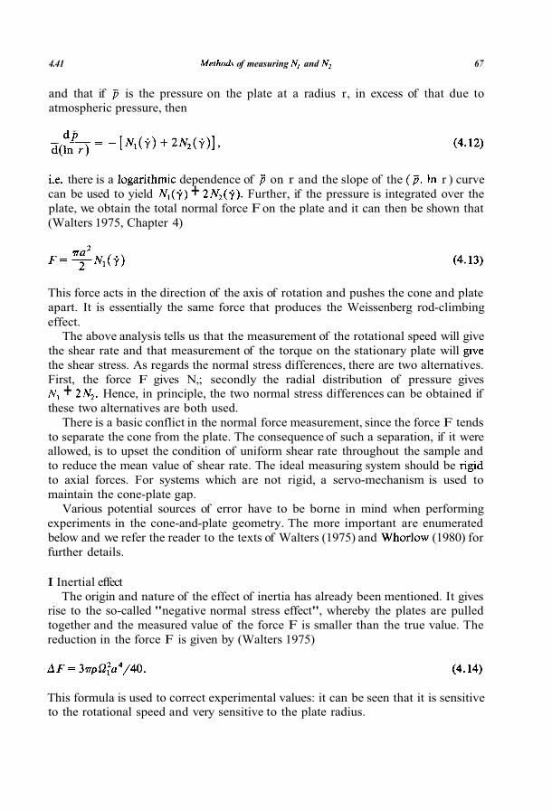
4.41 of measuring and 67

and that if is the pressure on the plate at a radius r, in excess of that due to

atmospheric pressure, then

there is a dependence of on r and the slope of the r ) curve

can be used to yield + Further, if the pressure is integrated over the

plate, we obtain the total normal force Fon the plate and it can then be shown that

(Walters 1975, Chapter 4)

This force acts in the direction of the axis of rotation and pushes the cone and plate

apart. It is essentially the same force that produces the Weissenberg rod-climbing

effect.The above analysis tells us that the measurement of the rotational speed will give

the shear rate and that measurement of the torque on the stationary plate will

the shear stress. As regards the normal stress differences, there are two alternatives.

First, the force F gives N,; secondly the radial distribution of pressure gives+ Hence, in principle, the two normal stress differences can be obtained if

these two alternatives are both used.

There is a basic conflict in the normal force measurement, since the force F tends

to separate the cone from the plate. The consequence of such a separation, if it wereallowed, is to upset the condition of uniform shear rate throughout the sample and

to reduce the mean value of shear rate. The ideal measuring system should be

to axial forces. For systems which are not rigid, a servo-mechanism is used to

maintain the cone-plate gap.

Various potential sources of error have to be borne in mind when performing

experiments in the cone-and-plate geometry. The more important are enumerated

below and we refer the reader to the texts of Walters (1975) and (1980) for

further details.

I Inertial effect

The origin and nature of the effect of inertia has already been mentioned. It givesrise to the so-called "negative normal stress effect", whereby the plates are pulled

together and the measured value of the force F is smaller than the true value. The

reduction in the force F is given by (Walters 1975)

This formula is used to correct experimental values: it can be seen that it is sensitiveto the rotational speed and very sensitive to the plate radius.


11 Hole-pressure error

A major source of error can arise when the pressure-distribution method is used is known as the hole-pressure error (Broadbent et al. 1968). Any method ofmeasuring pressure which relies on the use of a hole in the bounding surface gives alow result with elastic liquids owing to the stretching of the flow lines as they pass over the hole. The reduction is directly related to and is in fact used as a means of measuring N,. This method is described later in this chapter, where a more detailed description is given. The error is avoided by the use of stiff, flush-mountedpressure transducers.

111 Edge effects

"Shear fracture" places an upper limit on the usable shear rate range for highly

elastic materials like polymer melts. It is observed as a sharp drop in all stress components, and at the same time a change in shape of the free surface can be seen,as well as a rolling motion in the excess liquid around the rim of the plates. A horizontal free surface forms in the test sample at the rim and grows towards thecentre, hence reducing the sheared area. The limiting shear rate can be quite low,depending on the liquid and the cone dimensions. Expressed as a critical normalstress the limit is given by

where c is a constant of the liquid. For a given liquid, shear fracture is minimized ifthe cone radius and gap angle are small.

The name "shear fracture" was given to the effect by (1965) owing to itssimilarity to 'melt fracture', which limits the occurrence of steady flow of polymermelts in tubes. Tordella (1956) made the first systematic study of melt fracture andnoted that when the effect is severe the stream of melt breaks up with an

accompanying tearing noise.Another edge effect, also pointed out by (1972) is ascribable to changes

in contact angle and/or surface tension of the test liquid brought about by shear.

The effect is of potential importance when the test liquid possesses only small normal stresses.

IV Miscellaneous precautions

The alignment of the cone axis to be coincident with the rotational axis, thesetting of the cone tip in the surface of the plate, and the minimizing of, orcorrection for, viscous heating are other important matters to be taken into accountin accurate work.

4.4.2 Torsional

Torsional flow is shown schematically in Fig. 4.12 (see also Chapter 2). Clearly,commercial instruments which are designed to work in a cone-and-plate mode canbe easily adapted to the parallel-plate geometry and vice versa.

of measuring N, and

Stotionorv

II

plote

Fig. 4.12 Basic geometry for torsional flow.

In this case, with respect to suitably defined cylindrical polar coordinates, thevelocity distribution can be taken to be

= = = (4.16)

subject to the boundary conditions at the two plates

where h is the gap between the plates.Taking into account the fact that eqn. (4.16) is equivalent to a steady simple-shear

flow, the stress equations of motion are satisfied, with the shear rate given by

= (4.18)

provided

Equation (4.18) implies that the shear rate is independent of the viscometric

functions: it depends on radial distance r , but is constant across the gap for fixed r .

time, we see from eqn. (4.19) that we have to neglect inertia for compatibility

and there is no essential restriction on the gap h, except of that this must not

be too large that edge effects in a practical rheometer become important. The edge

effects mentioned in connection with the cone-and-plate instrument apply here.After some routine mathematics, it is possible to show that the viscosity function

can be determined from measurements of the torque through the equation (cf.

Chapter 2):

where is the shear rate at the rim ( r = a). It can also be shown that


where F is again the total normal force on the plates. We see that total-force data

yield the combination - at the shear rate at the rim. Clearly, total force

measurements taken in the cone-and-plate and parallel-plate geometries can be

combined to yield and separately. However, since is small and twoseparate experiments have to be performed, significant scatter in the final data can

be anticipated unless there is very refined experimentation.

Of interest is the fact that, in principle, relatively high shear rates can be attained

with small gaps h. This has been utilized in the so-called "torsional balance

rheometer" of Binding and Walters (1976) to obtain normal stress data at shear

rates in excess of In this form of the instrument, a predetermined external normal force is applied to the upper plate and the separation h is allowed to vary

until this force balances the normal force generated by the liquid. Gap h is

measured and eqns. (4.20) and (4.21) applied.

4.4.3 Flow through capillaries and slits

A consistent theory for normal stress measurement in flow through a capillary isavailable (cf. Walters 1975, Chapter 5), but this depends critically on the flow being

"fully developed" at the exit to the capillary, by which we mean that the Poiseuille

flow generated away from the influence of end effects should be maintained right up

to the capillary exit with no rearrangement of the velocity profile. Furthermore, the

experimental results have to be carried out with flush-mounted pressure tranducers

to avoid the hole-pressure error problem, and this is difficult on the curved walls of

a capillary. Therefore, the use of the potentially attractive exit-pressure measure-

ment technique of determining normal stress data is controversial (cf. Boger andDenn 1980). The associated jet-thrust technique for low viscosity elastic liquids and

high shear rates is also based on the assumption of fully developed flow at the

capillary exit (cf. Davies et al. 1975, 1977). In the Lodge (1988) stressmeter, which uses pressure-driven flow through a slit,

the hole-pressure error mentioned above is turned to good use in the measurement

of As liquid flows past the hole under an applied pressure gradient, streamlines

adjacent to the boundary wall are deviated into and then out of the hole, as shown

in Fig. 4.13. For an elastic liquid the deviation is viewed as a stretching by the

normal stress component acting along the streamlines. The net result is a lowering

of the pressure in the hole. The holes in the stressmeter are a pair of slots set across

the flow direction as shown in Fig. 4.13. The reduction in pressure A p is measured

Fig. 4.13 Schematic diagram of the Lodge stressmeter for normal stress and shear stress measurement.

The dotted lines represent the tension in the streamlines resulting in a lowered pressure in the holes.

Viscometric functions and linear functions 7 1

(as p, between the bottom of the hole beneath one of the slots and a

flush-mounted transducer whose diaphragm forms the boundary wall on the oppo-

site side of the slit. The difference in pressure in the two slots gives the

shear stress.

It has been shown theoretically that Ap is given by (cf. Tanner and 1969)

for a second-order simple-fluid model (which will be shown in $8.5 to be a valid

slow-flow approximation for a general class of elastic liquid). The generalization of

eqn. (4.22) embodied in the so called HPBL equation is used to interpret results for flows which are certainly outside the "slow-flow" regime. The interpretation of

results is accordingly based on what must be seen as an empirical equation, with no

theoretical justification except at low shear rates. However, it appears to work well,

judged by recent comparative studies with other instruments (Lodge et

and shear rates as high as have been reached with multigrade motor oils

with this technique.

4.4.4 Other flows

Tanner (1970) has proposed that the free surface shape in gravity-driven flow

down an open tilted trough can be used to calculate the second normal stress

difference In general terms, if the free surface rises near the centre, is

negative and, if it falls, is positive. The interpretation of data is not trivial, but

the technique provides a convenient method of determining estimates of at lowshear rates.

Circular Couette flow between rotating cylinders is popular in the determination

of the viscosity of non-Newtonian liquids (cf. $2.4). Attempts have also been madeto employ the flow to determine normal stress information from pressure readings

(Broadbent and Lodge 1972). The fact that the technique has not been popular with

experimentalists since the original paper is probably an indication of the difficulty

of using the technique, or it at least points to the fact that much easier methods are

available in rotational rheometry using, for example, cone-and-plate flow.

4.5 Relationships between viscometric functions and linear functions

Earlier in this chapter we argued that normal stress differences in a simple-shear

flow were a direct consequence of viscoelasticity. We recall from $3.5 that

can also be studied through a small-amplitude oscillatory-shear flow, theresulting stress distribution for an elastic liquid being expressible in terms of the

dynamic viscosity and the dynamic rigidity G'. Now, since the departure from a

Newtonian response in the viscometric functions and and in the dynamic functions and G' can be ascribed to viscoelasticity, we should not be surprised to

find that there are relationships between the various rheometrical functions. In fact,


Fig. 4.14 The Cox-Merz applied to the polymer solution which is a 2% polyisobutylene

(Oppanol solution in dekalin. 25 C.

it is not difficult to deduce the exact relationships in the lower limits of frequencyand shear rate:

The former relationship states that the viscosity measured in oscillatory shear in the zero-frequency limit is equal to the low shear viscosity measured in steady shear. Equation (4.24) is a relationship between the limiting values of dynamic rigidity andfirst normal stress difference.

In many cases, it is easier to carry out dynamic measurements than steady shear measurements and (4.23) and (4.24) provide a means of estimating the levels ofand (and hence from measurements of and G'.

We note that in view of eqn. (4.23) and the fact that both and are usuallymonotonic decreasing functions of and w, respectively, various attempts havebeen made to develop empirical relationships between and at other than thelower limits of shear rate and frequency. The most popular, and most successful inthis respect, certainly for polymeric liquids, is the so-called Cox-Merz (1958) rule,which proposes that should be the same function of as is of whereis the modulus of the complex viscosity,

4.51 Viscometric functions and linear functions

Fig. 4.15 A test of the relationshipof eqn. (4.24) showing the asymptotic approach of the oscillatory and

steady shear parameters. Steady shear and dynamic data for the polymer solution D3, which is a 1.5%

polyisobutylene solution in dekalin. 20 C.

In Fig. 4.14 we provide an example of the application of the Cox-Merz rule to a

polymer solution.In view of (4.24) and the fact that both G' and are monotonic increasing

functions of w and respectively, we might be led to expect that a relationshipanalogous to the Cox-Merz rule will hold between G' and (see, for example,

and cf. Al-Hadithi et al. 1988). The limiting relationship (4.24) has been

confirmed many times and Fig. 4.15 provides just one example of this for a

polymeric liquid, where we see that the values of and coincide at low

values of and w.

CHAPTER 5

EXTENSIONAL VISCOSITY

5.1 Introduction

The subject of 'extensional' (or 'elongational') flow received scant attention until

the mid Up to that time rheology was dominated by shear flows. In the last

twenty years or so the situation has changed dramatically with the dual realization

that extensional flow is of significant relevance in many practical situations and that

non-Newtonian elastic liquids often exhibit dramatically different extensional flow

characteristics from Newtonian liquids. Accordingly, interest in the subject has

mushroomed and much effort is now expended in trying to measure the extensional viscosity of non-Newtonian liquids, whether they be "stiff' systems like polymer

melts or "mobile" systems like dilute polymer solutions, suspensions and emulsions.

The general subject is covered in the book by (1979) entitled "Elongational

Flows Petrie's book requires more than a passing acquaintance with mathematics

to be fully appreciated, but there is sufficient general detail in the book to make it

important reading for anyone requiring a thorough knowledge of the subject. The

works of Dealy Meissner (1983, Miinstedt and Laun(1981, 1986) are also important sources of information for those whose direct

concern is polymer melts. Unlike the situation in steady simple shear and oscillatory shear (see Chapters

2-4) where the subjects are mature, the study of extensional flow is still evolving.

This is reflected in the slightly different style of the present chapter.

For the velocity field (see Fig.

where is a constant extensional strain rate, the corresponding stress distribution

can be conveniently written in the form

where is the (uniaxial) extensional viscosity. In general, it is a function of the

extensional strain rate just as the shear viscosity is a function of shear rate($2.3). However, we shall see that the behaviour of the extensional viscosity function

Extensional viscosity [Chap. 5

UNIAXIAL BIAXIAL PLANAR

EXTENSION EXTENSION EXTENSION

Fig. 5.1 The three different types of extensional flow fields are shown by the arrows: (a) Uniaxial; (b)

Biaxial; (c) Planar.

is frequently qualitatively different from that of the shear viscosity. So, for example,

highly elastic polymer solutions that possess a viscosity that decreases monotoni-cally in shear (showing shear-thinning) often exhibit an extensional viscosity that

increases dramatically with strain rate. A fluid for which increases with increasing is said to be 'tension-thickening',

whilst, if decreases with increasing it is said to be 'tension-thinning'.

Experimentally, it is often not possible to reach the steady state implied in (5.1)

and (5.2). Under these circumstances, it is convenient to define a transient exten-

sional viscosity i), which is clearly a function of t as well as This arises

from the obvious analogue to (5.2) given that the extensional flow field (5.1) is

initiated at time t = and maintained thereafter. In some respects this is adisappointing admission of difficulties which certainly do not normally occur in the

measurement of the shear viscosity However, a study of i ) can still

throw considerable light on the rheological response of non-Newtonian liquids. It isalso not without its industrial relevance, since in many practical situations liquids

are exposed to extensional flow fields over a limited period of time only (see, for

example, Bird et al. and Laun and Schuch 1988).

Another type of extensional deformation is the so-called biaxial extension, given

by (see Fig.

where is a constant. This type of extension is equivalent to stretching a thin sheet of material in two orthogonal directions simultaneously, with a corresponding

decrease in the sheet thickness. It is found (approximately) when a circular free jet

impinges on a flat plate or in a lubricated squeeze-film flow (see, for example, Soskey and Winter 1985) and when a balloon is inflated. The stress field corre-

sponding to (5.3) can be written in the form

Importance of extensional flow 77

where the biaxial extensional viscosity. It can be shown that (Walters 1975, p.

211)

Finally, a two-dimensional planar extensional flow given by (see Fig.

where i is a constant, yields a planar extensional viscosity

This type of extension is equivalent to stretching a thin flat sheet of material in one

direction only (the x direction), with a corresponding contraction in its thickness in

the z direction, but with no change in the width of the sheet. Planar extensional flow

can be shown to be equivalent to that generally known as "pure shear" (see, for

example, Walters 1975, Chapter 7).

In the present book, our general concern will be the uniaxial extensional viscosityand its comparison to the equivalent shear viscosity. Fuller details about subjects

not enlarged on here are provided in the texts of Petrie WaltersTanner (1985) and Bird et al. and (b)).

5.2 Importance of extensional flow

In polymer processing (see a case can be made out that some operations

involve a significant component of extensional flow, with the obvious conclusion

that the measurement of extensional viscosity may sometimes be as important as the

determination of the shear viscosity. This will become increasingly so as manufac-

turers attempt to further increase production rates.

Any reasonably abrupt change in geometry in a processing operation willgenerate a flow with an extensional component and, in particular, flows through asudden contraction or out of an orifice often lead to flow characteristics whichcannot be predicted on the basis of shear viscosity alone. The polymer engineer

must, therefore, have a working knowledge of extensional flow and must, if possible,know whether the materials he is processing are tension-thinning or

ing. Certainly, the 'spinnability' of a polymeric liquid can be very dependent on itsextensional viscosity behaviour. To illustrate this, consider the fibre-spinning pro-

cess shown schematically in Fig. 5.2. It is clearly important for the process, which is

dominated by extensional flow, to be stable and for the threadline not to snap. The

tension along the threadline is obviously chosen to prevent fracture under normal operating conditions and the main concern is with the propagation and magnifica-

tion of small disturbances, which are to some extent unavoidable in a physical

process of sort.

78 [Chap. 5

From thespinnerette

Fig. The filament-necking imperfection in fibre spinning.

The stability of a spinning threadline is a vast area of study (see, for example,

Petrie 1979) and we shall do no more than isolate one possible cause for concern.Let us speculate that for some reason a change in diameter occurs. From simple

continuity considerations we would expect the narrower part of the filament to

move faster than the rest of the threadline. Put in another way, the extensionalstrain rate will now be higher in the narrow part. If the polymeric liquid is

tension-thinning, the resistance to extension is reduced in the narrow part and

motion in this part of the threadline is further accelerated. It becomes thinner and

may ultimately break.

If, on the other hand, the polymeric liquid is tension-thickening, the resistance in

the narrow part of the filament will now be increased. The flow in the filament will

slow down, the radius will increase and may be expected to return to that of the

remainder of the threadline. Tension-thickening is therefore a stabilizing influence

in this process.

Other examples of the importance of extensional viscosity in polymer processingcould be cited. Certainly, the polymer engineer needs to be aware of the fact that

two polymeric liquids which may have essentially the same behaviour in shear can

show a different response in extension.Later in this chapter we shall see that there is sufficient theoretical and experi-

mental evidence available to support the view that very dilute solutions of flexible

polymers can have extremely high extensional viscosities. Certainly, these can be

orders of magnitude higher than those expected on the basis of Newtonian theory.This has important consequences in a number of practically important situations.

For example, it may significantly affect the pressure losses encountered in polymer

flooding in "enhanced oil recovery" (EOR) (see Further, it may be the

cause of the phenomenon known as "drag reduction". When small concentrations

Importance of extensional flow

Fig. 5.3 The 4-roll mill experiment. Schematic representation of the fluid velocities for: (a) A Newtonian

liquid; (b) A highly elastic liquid, for which high extensional stresses at A and B reduce the inflow.

(of the order of a few parts-per-million) are added to a Newtonian solvent like water, there is often a substantial reduction in drag in turbulent flow (Tanner 1985,

p. 423). Drag reduction is of potential importance in many spheres. For example,

small quantities of polymer may be injected into sewers during heavy rain to

upgrade flow and so prevent flooding.

Many different mechanisms have been proposed to account for the phenomenon

of drag reduction, but it may be linked to extensional viscosity and in particular to

the suppression of the roll-wave motion and vortex stretching in the by the

high extensional viscosity.

The potential importance of extensional viscosity effects in such processes as calendering and paper coating is suggested by the four-roll mill experimentsdiscussed by Metzner and Metzner (1970) (see Fig. 5.3).

When the four-roll mill is immersed in a Newtonian liquid, the expected flowregime shown in Fig. is observed. However, in the case of some dilute

polymer solutions, the flow shown in Fig. more adequately reflects the

observations. The flow at A and B is too "strong" to permit substantial amounts offluid to enter as in Fig. Specifically, the anticipated flow has a high

extensional component which results in high extensional stresses. The shear stresses

generated by the rotating rollers are not strong enough to overcome the large extensional stresses and a reversed flow results at A and B.

Further examples of anomolous flow characteristics caused by high extensional

viscosities are given in

80 Extensional [Chap. 5

Finally, we remark that extensional flow experiments can be viewed as providing

critical tests of any proposed constitutive equations. Indeed, the historical conven-tion of matching only shear flow data with theoretical predictions in constitutive

modelling may have to be rethought in those areas of interest where there is a large

extensional contribution. It may be more profitable to match any extensional

viscosity data which may be available, even if this means that the resulting constitutive model loses some of its predictive value so far as shear data are

concerned.

5.3 Theoretical considerations

Continuum mechanics is able to provide some useful insights into the exten-

sional-viscosity behaviour of non-Newtonian liquids. For example, the following

limiting relations between extensional and shear viscosities are true (cf. Walters

1975, Petrie 1979)

We note that these relationships are valid for all values of and in the case of

Newtonian liquids. In particular, for Newtonian liquids,

a result obtained by Trouton as early as 1906. Accordingly, rheologists have

introduced the concept of the 'Trouton ratio' defined as

Elastic liquids are noted for having Trouton ratios, but the definition as givenin eqn. (5.11) is somewhat ambiguous, since it depends on both and and some

convention has therefore to be adopted to relate the strain rates in extension and

shear. To remove this ambiguity and at the same time provide a convenient estimate of viscoelastic effects, Jones et al. (1987) have proposed the following definition,

based on a simple analysis for an inelastic non-Newtonian fluid:

in the denominator, the shear viscosity is evaluated at the shear rate numerically

equal to Jones et show that if the fluid is inelastic and isotropic, is 3 for

Theoretical considerations 81

values of i . They argue that any departure from the value 3 can be associated

unambiguously with viscoelasticity, so that the definition (5.12) not only removes the ambiguity in the definition of the Trouton ratio, but also provides a convenient

means of estimating viscoelastic response.Variable (shear) viscosity effects are accommodated in the analysis of Jones et al.,

which illustrates convincingly that a fluid that is shear-thinning must also be

expected to be tension-thinning in extension, if uiscoelastic effects are negligible or

very

Continuum mechanics also supplies a limiting relationship between the exten-

sional viscosity and the normal stress coefficients and as determined in

shear flow. A simple analysis for the so-called second-order model (which is argued

in $8.5 to provide a general description of non-Newtonian behaviour in sufficiently

slow flow) leads to the following relation:

Available experimental evidence from shear-flow rheometry (cf. $4.2) would indi-

cate that

so we expect

for non-Newtonian elastic liquids. This is important, since it indicates that theextensional viscosity must be an increasing function of for very small values of

initial tension-thickening must be anticipated for all elastic liquids satisfying

whatever the response at higher values of i may be. Bird (1982) has made the interesting observation that it is usually easier to

calculate theoretically the extensional flow characteristics of molecular models than

the corresponding shear flow functions. He has also provided a useful summary of

the predictions for various molecular models of polymeric liquids. Many of thempredict infinite extensional viscosities at a finite value of the extensional strain rate

(cf. the predictions in Table 8.3). Partly to overcome this problem, Phan Thien and

Tanner (1977) proposed a model which allows to pass through a maximum

rather than take infinite values. For general and future interest, we show in Fig. 5.4

schematic and curves computed for the so-called PTT model. Interestingly,

although the initial values of and are different at low strain rates, in

agreement with eqns. (5.8) and they are indistinguishable at high strain rates.

The general observation concerning the relative ease of carrying out theoretical

work on the extensional flow characteristics of molecular models is also illustrated

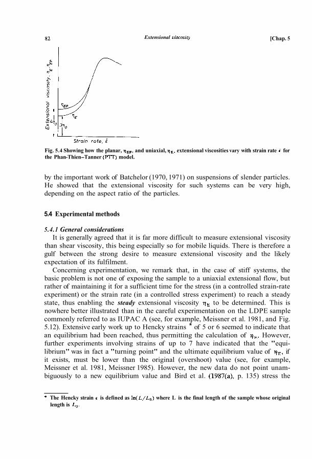
Extensional [Chap. 5

Fig. 5.4 Showing how the planar, and uniaxial, extensional viscosities vary with strain rate for

the Phan-Thien-Tanner model.

by the important work of Batchelor (1970, 1971) on suspensions of slender particles. He showed that the extensional viscosity for such systems can be very high,

depending on the aspect ratio of the particles.

5.4 Experimental methods

5.4.1 General considerations

It is generally agreed that it is far more difficult to measure extensional viscosity

than shear viscosity, this being especially so for mobile liquids. There is therefore a

gulf between the strong desire to measure extensional viscosity and the likely

expectation of its fulfilment.

Concerning experimentation, we remark that, in the case of stiff systems, the

basic problem is not one of exposing the sample to a uniaxial extensional flow, butrather of maintaining it for a sufficient time for the stress (in a controlled strain-rate

experiment) or the strain rate (in a controlled stress experiment) to reach a steady

state, thus enabling the steady extensional viscosity to be determined. This is

nowhere better illustrated than in the careful experimentation on the LDPE sample

commonly referred to as IUPAC A (see, for example, Meissner et al. 1981, and Fig.5.12). Extensive early work up to Hencky strains * of 5 or 6 seemed to indicate that

an equilibrium had been reached, thus permitting the calculation of However,

further experiments involving strains of up to 7 have indicated that the "equi-

librium" was in fact a "turning point" and the ultimate equilibrium value of if

it exists, must be lower than the original (overshoot) value (see, for example,Meissner et al. 1981, Meissner 1985). However, the new data do not point unam-

biguously to a new equilibrium value and Bird et al. p. 135) stress the

The Hencky strain is defined as where L is the final length of the sample whose original

length is

5.41 Experimental 83

general difficulty of reaching a steady state in extension for many polymer melts,

questioning whether a meaningful extensional viscosity exists for some materials

and conditions. Fortunately, a knowledge of the transient function may be

sufficient (or at least very useful) in many practical applications (cf. Bird 1982,

Laun and Schuch, 1988). When it is realized that the Hencky strain of 7 reached in the Meissner

experiments corresponds to stretching the sample to times its original length,

the difficulties involved in extensional rheometry become self-evident.

The problems of determining the extensional viscosity of mobile liquids are evenmore acute, but they are of a different type from those experienced for stiff systems.

With mobile liquids, severe difficulties arise in trying to achieve a continuous

extensional flow field which approximates that given in eqs. (5.1). The most that one

can hope for is to generate a flow which is dominated by extension and then to

address the problem of how best to interpret the data in terms of material functions

that are rheologically meaningful.Fortunately, for many mobile elastic liquids, the extensional viscosity levels are

so high (and potentially important) as to justify such an approach. This fact has

spawned a number of extensional rheometers in recent years and most of them are

able to capture the high extensional viscosities which are known to exist. The main

outstanding problem is to assess critically the viscosities" arising from the various

methods and to see whether a concensus emerges. This is under active consideration

(Walters 1988).

5.4.2 Homogeneous stretching method

The homogeneous stretching method, illustrated in Fig. 5.5, was the first to be

used to determine the extensional viscosity.

A major (unavoidable) disadvantage of this method is that, in order to attain aconstant extensional strain rate in the sample, the velocity of the movable block

must vary exponentially with time. In principle this can now be accomplished veryeasily with the most recent electronic-control techniques, but the accelerating

motion of the clamp places a severe constraint on the strain rates can be

attained, given the requirement that the motion must be sustained for a sufficient

time for the stress (which is measured at either the stationary or the moving block)

to reach a steady value.

For practical reasons the overall deformation is clearly restricted in the conven-

tional stretching method of Fig. 5.5. The Meissner (1972) apparatus shown in Fig.5.6 goes some way to overcoming this problem (see also Laun and Miinstedt 1978).

Instead of end loading, constant stretching is provided by two sets of toothed wheels

block test block

Fig. 5.5 Schematic diagram of the homogeneous stretching method.


Fig. 5.6 Schematic diagram of the Meissner apparatus for attaining high strains (see, for example,

Meissner 1972). Note that the stretched specimen is supported by a suitable liquid.

which rotate with constant angular velocity. The stress can be measured by the

deflection of a spring F, associated with one pair of rollers.

Using this method on polymer melts, Meissner (see, for example, Meissner 1985) has been able to reach Hencky strains as high as 7. A further recent development

has involved the use of a series of clamps in the form of a ring. In this way other

modes of (multiaxial) extensional deformation can be generated (Meissner 1985).

The homogeneous stretching method is clearly restricted to high-viscosity sys-

tems.

5.4.3 Constant stress devices

The instruments shown schematically in Figs. 5.5 and 5.6 are of the constant

strain-rate type. An alternative technique, first introduced by (1968) and

developed later by Miinstedt (1975, 1979) utilizes a constant stress, is brought

about by applying a force to the movable block in Fig. 5.5, the force decreasing in

proportion to the cross-sectional area of the extending specimen. exployed

this method using a cam to apply a programmed load, together with a convenient

means of measuring the length of the sample as a function of time.

It is interesting to note that as a general rule the constant stress devices reach thesteady-state elongational flow regime at smaller total deformations than the con-

stant strain-rate devices. For example, Laun and Schuch (1989) quote that a strain

of 3.5 was required to reach equilibrium in a constant stress experiment on anLDPE melt whereas a strain of 4.5 was required in the comparable constant

strain-rate experiment.

The constant stress devices are also clearly restricted to high-viscosity systems.

5.4.4 Spinning

It is self-evident that fibre spinning involves a significant extensional-flow

component. At the same time, it is extremely difficult (if not impossible) to interpret

Experimental

Die swell

Test section

Wind- up 'or suctiondevice

Fig. 5.7 Schematic diagram of the spin-line rheometer

the data unambiguously in terms of the extensional viscosity defined in eqns.(5.2). The problem is that, although the flow may be steady in an Eulerian sense (in

that the velocity at a fixed distance down the threadline does not vary with time) it

is unlikely to be steady in a Lagrangian sense (since the strain rate experienced by a

given fluid element will generally change as it moves along the threadline). Further-more, even when the strain rate is constant over a portion of the threadline (so that a

given fluid element is exposed to a constant strain rate for a limited period of time)

that element may still "remember" conditions experienced in the reservoir in the

case of highly elastic liquids. Certainly, there is ample evidence that a change ofconditions in the spinnerette can significantly affect the response along the

line under some conditions. The fibre-spinning experiment (Fig. is therefore a typical illustration of the

dilemma facing rheologists who are interested in extensional-viscosity measurement. It is relatively easy to perform, the general kinematics can be determined with

relative ease, and a suitable stress variable can be obtained from force measure-

ments on the reservoir or the take-up device (see, for example, Hudson and

Ferguson 1976, Jones et al. 1987). However, a consistent quantitative interpretation

of the experimental data in terms of the extensional viscosity defined in eqns.

(5.2) is not possible. One can certainly define an extensional viscosity by dividing

the measured stress by (say) an average value of the strain rate (Jones et al. 1987).

Given the difficulties encountered in measuring extensional viscosity and the scale

86 Extensional [Chap. 5

of the viscoelastic response in such a flow, the proposed course of action can be

justified and may be all that is required in many circumstances.

The spinning technique can be used for polymer melts (see, for example, Laun

and Schuch 1989) and for low viscosity liquids (Jones et al. 1987). In the commercial

spin-line rheometer (see, for example, Ferguson and El-Tawashi 1980) the wind-updevice is a rotating drum. A variant of this for very mobile liquids is to use a suction

device (Gupta and Sridhar 1984).

5.4.5 Lubricated flows

A schematic diagram of the lubricated-die rheometer is given in Fig. 5.8. The

shape of the test section is so designed that the flow is equivalent to steady

extensional flow there is perfect slip at the walls. To facilitate this, lubricantstreams of low-viscosity Newtonian liquids are employed. Pressure measurements

provide the relevant stress input.

This would seem to be a convenient technique for eliminating the unwanted

shearing induced by the rheometer walls, thus providing a flow close to the desired

extensional flow. However, the interface boundary condition between the sample

and the lubricant is dependent on the rheological properties of the sample. The

interpretation of experimental data is therefore not without its problems and the

technique itself is far from easy to use (see, for example, Winter et al. 1979,

Williams and Williams 1985, Jones et al. 1987).

A similar technique has also been used by Winter (see, for example, Soskey and

Winter 1985) to study biaxial extensional flows of polymer melts. In this case

uniform discs of the sample are placed between two parallel circular plates, both of

Fig. 5.8 Schematic diagram of the lubricated-converging-flow rheometer; the shape of the channel walls is

chosen such that the flow is equivalent to a pure extensional flow if the low-viscosity lubricant streams

are able to bring about "perfect slip" at the walls.

5.41 Experimental 87

which are coated with a low-viscosity lubricant. The plates are then squeezedtogether. The relationship between applied load and rate of squeezing is interpretedin terms of the extensional viscosity Again, data interpretation isdifficult and the technique itself is not easy to use.

5.4.6 Contraction flows The contraction-flow method of determining extensional properties can be ap-

plied equally well to polymer melts and to more mobile systems like dilute polymersolutions. Indeed, in the case of polymer melts, the so-called (1957) correc-tion (or a suitable variant of it) must be used to interpret correctly shear viscositydata from a capillary rheometer (cf. The correction can be im-mediately utilized to yield extensional-viscosityinformation on the melt, as we shallsee. Specifically, in capillary rheometry where the test fluid is forced to flow underpressure from a barrel into a capillary of much smaller radius, one technique is tomeasure the pressure in the barrel for fixed capillary diameter D and varying lengthL (cf. Chapter 2 and Fig. 5.9). At a fixed flow rate, a plot of pressure as a function of L/D provides sufficient information to facilitate shear-viscosity determination: in particular, the pressure drop for fully developed Poiseuille flow along a capillary of a given length can be determined.

Often, just two experiments are carried out in capillary rheometry: one for a capillary of a reasonable length 20) and the other for so-called orifice flow

L = It is this last experiment (and by implication the correction)which is of potential importance in the determination of extensional-viscositycharacteristics.

In general, a contraction geometry is simply two capillaries of different diameters with an abrupt contraction between them. In some experiments, as we haveindicated, flow through an orifice is an alternative.

Usually, but not always, the flow consists of a central core and a vortex region(see Fig. 5.10). The kinematics are determined by the flow rate and the shape of thecentral core region, whilst the relevant stress is obtained from the pressure droprequired to force the test fluid through the contraction. There is no doubt that the

0

Fig. 5.9 The correction. The pressure drop (for a fixed flow rate and fixed capillary diameter) is

measured for various values of capillary length.


NEWTONIAN

VISCOELASTIC

Fig. 5.10 Contraction flow. In the case of highly elastic liquids, vortex enhancement usually occurs.

contraction-flow experiment is relatively easy to perform and has many attractive

features.An approximate analysis of the contraction-flow problem has been developed by

Binding (1988). This extends and reinterprets the early analysis of

and (b)). The Binding analysis is based on the assumption that the flow field is the

one of least resistance; it includes both shear and extension in its formulation. Thetheory successfully predicts the phenomenon of vortex enhancement, which is often

observed in axisyrnmetric contraction flows, and provides estimates of the exten-

sional viscosity.

5.4.7 Open-syphon method

The open-syphon technique is shown schematically in Fig. 5.11. Fluid from the reservoir is drawn up through a nozzle by a vacuum pump and the nozzle is then

raised above the level of the liquid in the reservoir. With some liquids the upward

flow continues. This is the open-syphon effect. The flow rate and the dimensions of

the fluid column yield the relevant kinematical information and the stress is

provided by force measurements made at the top of the liquid column (see, forexample, Astarita and Nicodemo 1970, Moan and Magueur 1988).

In general terms, the open-syphon technique suffers from the same general

disadvantages as the spinning experiment, so far as data interpretation is concerned. However, the former may have advantages in the case of structured materials like

gels. In the spinning experiment the structure is often changed by shear in the

delivery pipe. In contrast, the test material in the open-syphon technique is in its

Experimental results

Fig. 5.11 The open-syphon technique for studying extensional flow. Liquid is sucked up from the

reservoir into a tube, and the downward pull on the tube is measured.

rest state before being exposed to a sudden extension and one is therefore ing what is essentially a measure of the extensional properties of the virgin gel.

5.4.8 Other techniques

Numerous other techniques have been suggested for the study of the extensional behaviour of mobile elastic liquids. These include the so-called triple-jet technique

(Oliver and the droplet techniques of Schiimmer and and

Jones and Rees the elongation of radial filaments on a rotating drum (Jones

et al. 1986) and stagnation-point devices such as the opposing-jet techniques of

et al. Keller and (1985) and Fuller et al. (1987).

5.5 Experimental results

Typical transient extensional-viscositydata for a polymer melt are given in Fig.5.12 (cf. Meissner 1985, Bird et al. It will be seen that as the strain rate is

increased, the experimental results depart from "Trouton behaviour" *, increasingabruptly with time. This is called "strain hardening". There then follows the

maximum in already referred to in In view of the extreme difficulty

* Trouton behaviour, in this context, is obtained from linear viscoelasticity theory.

90 Extensional viscosity [Chap. 5

Time, t / s

Fig. 5.12 Extensional growth 2 ) as a function of time t for a low-density polyethylene

melt. 423 K (see, for example, Meissner 1985).

of obtaining data at relatively high strains, rheologists nowadays often simply quote

the maximum values of i)(which were, of course, once thought to be the

equilibrium values When this is done, one obtains the type shown

in Fig. 5.13 for four polymer melts. The data are consistent with the requirements of

eqs. (5.8) and (5.15). There is a clear indication of a maximum in with strain rate

for the polyethylenes.If the extensional viscosity and shear viscosity are plotted as functions of stress,

,

CHDPE 2

, ,

rote,

Fig. 5.13 Extensional viscosity data for four polymer melts (after Laun and Schuch 1989).

LDPE-low-density polyethylene; HDPE-high-density polyethylene; PS-polystyrene.

0

LDPE 9

5.51 Experimental results

I

-IUPAC A

10 10Stress, Pa

Fig. 5.14 Extensional viscosity and shear viscosity as functions of stress for the low-density polyethelyne

designated IUPAC A. 423 K (cf. Fig. 5.12) (see, For example, Laun and Schuch 1989).

rather than strain rate, the response shown in Fig. 5.14 is obtained for a typical

low-density polyethylene melt.

In Fig. 5.15 we show extensional-viscosity data obtained from a spin-line

rheometer on a solution of polybutadiene in dekalin (Hudson and Ferguson 1976).

Here there is a further and substantial increase in after the tension-thinning

region. The data in Figs. 5.13 and 5.14 do not extend to sufficiently high values of

to indicate whether the ultimate tension-thickening trend occurs also for stiff

polymeric systems.

We have already indicated that the accurate determination of for mobile

elastic liquids is very difficult, perhaps impossible, but the evidence to handindicates that the extensional viscosities which have been measured can be very high

indeed. For example, in Figs. 5.16 and 5.17 we show shear- and extensional-viscosity

r a t e .

Fig. 5.15 Extensional viscosity curve determined with a commercial spin-line rheometer for a 6.44%

solution of polybutadiene in dekalin (cf. Hudson and Ferguson 1976).


Fig. 5.16 Viscometric data for aqueous solutions of polyacrylamide (1175 grade) (Walters and Jones

1988). Note that viscosity decreases and normal stress increases with shear rate.

10'

Strain rote.

Fig. 5.17 Extensional viscosity data obtained from a spin-line rheometer for the aqueous polyacrylamide

solutions of Fig. 5.16 (Walters and Jones 1988). Note that whereas shear viscosity decreased with shear

rate, extensional viscosity increases with extensional rate.

Experimental results

3 % XANTHAN SOLN.

.

rote.

Fig. 5.18 Viscometric data for a 2% aqueous solution of polyacrylamide grade) and a 3% aqueous

solution of Xanthan gum. Note the very different values of for solutions with almost the same

viscosities.

2% POLYACRYLAMIDE

3% XANTHAN

I I

rote. rote,

Fig. 5.19 (a) Extensional viscosity data obtained from a spin-line rheometer for the polymer solutions

investigated in shear flow in Fig. 5.18; (b) Trouton ratios obtained from Figs. 5.18 and Note that

although the Xanthan gum solution is tension-thinning (Fig. the associated Trouton ratios

increase with strain rate and are still significantly in excess of the inelastic value of 3.


data for a series of very dilute aqueous solutions of a very high molecular-weightpolyacrylamide designated 1175 (Walters and Jones 1988). It is not difficult to

deduce that the Trouton ratios are as high as

We now refer to the rheometrical behaviour of two polymer solutions with almostidentical shear viscosity behaviour (see Figs. 5.18 and 5.19). One is a 2% aqueous

solution of polyacrylarnide grade) and the other a 3% aqueous solution of

Xanthan gum. We note that polyacrylamide is a more flexible polymer than

Xanthan gum which is rod-like. The corresponding extensional-viscosity data ob-

tained from a spin-line rheometer show that the polyacrylamide solution is strongly

tension-thickening, whereas the Xanthan gum solution is tension-thinning over the

Fig. 5.20 An illustration of the open-syphon effect for a 0.75%aqueous solution of polyethylene oxide.

5.61 High extensional viscosity behaviour 95

range studied. However, when the Trouton ratios are calculated on the basis of eqn.we see that even the Xanthan gum solution has values that are signifi-

cantly higher than the Newtonian value of 3 over most of the range.Finally, we note that available evidence would indicate that the Trouton ratios

for non-polymeric colloidal liquids are much lower than those for polymeric liquids showing similar behaviour in small-amplitude oscillatory-shear flow.

5.6 Some demonstrations of high extensional viscosity behaviour

We conclude this chapter by referring to some easily reproduced situations inwhich the dramatic effects of high Trouton ratios are clearly in evidence. Some ofthese can be readily performed in the laboratory with quite standard equipment.

We have already referred to the open-syphon technique for measuring exten-sional viscosity (cf. We remark that the use of a 0.75% aqueous solution ofpolyethylene oxide WSR 301 grade (or similar polymer solution) will enable the experimenter to operate a conventional syphon several centimetres above the levelof the reservoir liquid.

The open-syphon effect is even more dramatically demonstrated when thepolymer solution is transferred from one full container to a lower empty container. All that is normally required to (almost) empty the container is to start the flow byslightly tilting the top container. The initial flow will be sufficient to empty the bulk of the liquid from the top container (see Fig. 5.20). The open-syphon phenomena can be directly attributed to the very high Trouton ratios exhibited by the polymersolution. These and other dramatic demonstrations of high extensional-viscosity

behaviour are illustrated in the film "Non-Newtonian Fluids" produced by Waltersand Broadbent (1980) *.

Our final example of visual extensional-viscosity phenomena is provided by flow

past cylindrical obstructions placed asymmetrically in a parallel channel (cf. Waltersand Jones 1988). The flow is basically two-dimensionaland may be considered to bemade up of narrow channels and wide channels formed by the offset positioning of

the circular-cylinder barriers (Fig. 5.21).The behaviour of the Newtonian liquid is unspectacular with as much liquid

going through the narrow channels as one would expect. This behaviour may be contrasted with that for the relatively inelastic Xanthan gum solution. In this case, asubstantial flow finds its way through the narrow channels, clearly on account of theshear-thinning viscosity.

Finally, we note the qualitative difference in the behaviour of the highly elasticshear-thinning polyacrylamide solution. In this case, extensional viscosity consider-

* The film is available in Video or form from the Department of Mathematics, University College

of Wales, UK.


Fig. 5.21 Flow visualization pictures for: (a) a Newtonian liquid; (b) a Xanthan gum solution; (c) a

polyacrylamide solution. They show the dominant effects of shear-thinning in the Xanthan gum solution

and tension-thickening in the polyacrylamide solution (see, for example, Walters and Jones 1988).

are all important and virtually no liquid finds it way into the narrow

channels. There is a relatively fast-moving stream in the wide channels and virtually

stagnant regions elsewhere (cf. the four-roll mill situation in Fig. 5.3).

CHAPTER 7

RHEOLOGY OF SUSPENSIONS

7.1 Introduction

The rheology of suspensions has been the subject of serious research for many

years, mainly because of its obvious importance in a wide range of industrial

applications (see, for example, Barnes 1981). Suspensions include cement, paint,

printing inks, coal slurries, drilling muds and many proprietory products like

medicines, liquid abrasive cleaners and foodstuffs. Examples of suspensions where

the particles are deformable range from emulsions to blood.

7.1.1 The general form of the viscosity curve for suspensions

The general rate curve for all suspensions is shown schematically

in Fig. 7.1. We could anticipate most of this behaviour from the general discussion of Chapter 2. The first Newtonian plateau at low shear rate is followed by the

power-law shear-thinning region and then by a flattening-out to the upper (second)

Newtonian plateau. At some point, usually in this upper Newtonian region, there

can be an increase in viscosity for suspensions of solid particles, given the ap-propriate conditions. In certain situations the first Newtonian plateau is sometimes

so high as to be inaccessible to measurement. In such cases the low-shear ratebehaviour is often described by an apparent yield stress.

The factors controlling the details of the general flow curve in particular cases

will now be considered. One point worth stressing here is that the relevant measure

of the amount of material suspended in the liquid is that fraction of space of the

Log rote

Fig. 7.1 Schematic representation of the flow curve of a concentrated suspension.

116 of suspensions [Chap. 7

total suspension that is occupied by the suspended material. We call this the phase

volume This is the volume-per-volume fraction, and not the weight-per-weight

fraction that is often used in defining concentration. The reason why phase volume

is so important is that the rheology depends to a great extent on the hydrodynamic

forces which act on the surface of particles or aggregates of particles, generally

irrespective of the particle density.

7.1.2 Summary of the forces acting on particles suspended in a liquid

Three kinds of forces coexist to various degrees in flowing suspensions. First,

there are those of colloidal origin that arise from interactions between the particles.

These are controlled by properties of the fluid such as polarisability, but not by

viscosity. These forces can result in an overall repulsion or attraction between the

particles. The former can arise, for instance, from like electrostatic charges or fromrepulsion of polymeric or surfactant material present on the particle

surfaces. The latter can arise from the ever-present London-van der Waals attrac-

tion between the particles, or from electrostatic attraction between unlike charges on different parts of the particle attraction between clay particles). If

the net result of all the forces is an attraction, the particles flocculate, whilst overall

repulsion means that they remain separate dispersed or deflocculated).

Each colloidal force has a different rate of decrease from the surface of the

particle and the estimation of the overall result of the combination of a number of

these forces operating together can be quite complicated. Figure 7.2 shows the form

of some single and combined forces (see Hunter 1987 for a more detailed account of

colloidal forces).Secondly, we must consider the ever-present Brownian (thermal) randomising

force. For particles of all shapes, this constant randomisation influences the form of

the radial distribution function the spatial arrangement of particles as seen fromthe centre of any one particle), whereas for non-spherical particles, spatial orienta-

tion is also being randomised. The Brownian force is of course strongly

dent, so that below a particle size of 1 it has a big influence. This force ensures

that the particles are in constant movement and any description of the spatial

distribution of the particles is a time average.

Thirdly, we must take into account the viscous forces acting on the particles. The

viscous forces are proportional to the local velocity difference between the particle

and the surrounding fluid. Hence the way these affect the suspension viscosity

enters via the viscosity of the continuous phase which then scales all such interac-

tions. Thus an important parameter is the 'relative viscosity' defined as thesuspension viscosity divided by the continuous-phase viscosity.

Clearly, the rheology measured macroscopically is strongly dependent on these

microstructural considerations. For instance, the presence of isolated particles means deviation of the fluid flow lines and hence an increased viscosity. At higher

concentrations, more resistance arises because particles have to move out of each

other's way. When particles form flocculated structures, even more resistance is encountered because the by enclosing and thus immobilising some of the

7.11 Introduction

Fig. 7.2 Examples the typical interaction Forces between a pair of sub-micron particles: (a) van der

attraction (omnipresent); (b) Steric repulsion due to adsorbed macromolecules; (c) Electrostatic

repulsion due to the presence of like charges on the particles and a dielectric medium; (d) A combination

of (a) and (b); (e) A combination of (a) and (c); (f) A combination of (a), (b) and (c).

continuous phase, have the effect of increasing the apparent phase volume, thus

again giving a higher than expected viscosity.

7.1.3 Rest structures

When particles are introduced into a liquid at rest they usually assume a state of

thermodynamic equilibrium which, when the Brownian motion dominates, corre-

sponds to a random disordered state. When colloidal forces dominate, the particles form structures whose forms

depend on whether the overall forces are attractive or repulsive. When they are

attractive they form aggregates and when they are repulsive they form a

pseudo-lattice.The particular shape of aggregates can vary from near-spherical flocs to strings.

The latter is sometimes referred to as a string-of-pearls structure. Pigment disper-

sions form flocs and silica dispersions can form the string structures.

Pseudo-lattices are formed by overall repulsion, for instance in systems ofparticles carrying electrostatic charges of the same sign dispersed in a polar

continuous phase. The particles then take up positions as far from each other as

possible. If the charge on such particles is very large, movement of the particles is

severely restricted and the structure can be visualised as a pseudo-crystal: if the

lattice spacing is comparable to optical wavelengths, interference effects occur and

the suspension displays irridescence.

of suspensions [Chap. 7

Any of the structures mentioned above can be modified by the adsorbtion ofsurfactant materials onto the surface of the particles. The structures formed by

electrostatic charges can be modified by the addition of electrolytes.The structures discussed so far are formed by near-spherical particles. However,

if the basic particle is itself anisotropic, very complicated structures can be formed.

One example is an aqueous suspension of bentonite clay: the basic particle is

plate-like and it carries charges of opposite sign on the faces and edges. The

aggregated structure is then like a house of cards with edges attracted to faces.Another example is a suspension of soap crystals. Soap can be made to crystallize in

the form of long ribbons, which then intertwine to form an entangled structure, as

in lubricating grease.

A useful method for judging the importance of colloidal forces has been derived

by Woodcock (1985). It gives the average distance between first neighbours interms of the particle size d and the volume fraction as follows:

This expression is plotted in Fig. 7.3 for four sizes of particle. The diagram also

shows the range of action of typical colloidal forces. This diagram indicates for

example that, for a suspension with a of 0.2 and particle size 0.05 electro-

static interactions will be very important. This will not be so if particles are larger orif the concentration is lower.

0.2 0.3 0.5 0.6 0.7Solids volume fraction

Fig. 7.3 Average interparticle separation as a function of concentration for monodisperse spheres

(according to eqn. (7.1)) plotted for four particle sizes. The horizontal lines show twice the distance over

which various interparticle forces typically operate: (A) Electrostatic forces in aqueous suspensions with

low salt levels; (B) Steric forces originating from adsorbed macromolecules; (C) Steric forces originating

from adsorbed detergents.

Solid particles in Newtonian liquids 119

7.1.4 Flow-induced structures

We shall consider first, relatively unaggregated systems in which the Brownian

forces dominate. When a concentrated suspension of this type flows at very low

shear rates, the particles necessarily have to move around each other or "bounce

off' each other for overall flow to occur. This involves a large resistance and the

resulting viscosity is On the other hand, the distribution of particles remains

essentially undisturbed because the effect of Brownian motion dominates the shear motion and restores the randomness of the rest-state distribution. The viscosity

remains essentially constant. At slightly higher shear rates, the imposed velocity

gradient induces an orientation of the particle structure, which is not restored by the

Brownian motion. However this orientation enables particles to move past each

other more freely than at very low shear rates and hence the viscosity is lower. At

even higher shear rates, the structure is so grossly orientated that the particles form

layers separated by clear layers of the continuous phase. The viscosity is then at itsminimum value. The suspension is shear-thinning. The existence of particle layers

has been confirmed by light diffraction. When shearing is stopped the flow-induced

layered structure gradually disappears.

If the shear stress is increased above a critical value, the layers disrupt and

gradually disappear. Hence, the viscosity begins to rise again and it also increases

with time of shearing.Flow-induced structures can also be formed by the more complicated clay and

soap suspensions mentioned earlier. In these cases, flow causes the plates and

ribbons to align in the direction of flow. This orientation can be detected by optical

techniques.Examples of increased flocculation caused by flow are also known (see, for

example, Cheng 1973).

7.2 The viscosity of suspensions of solid particles in Newtonian liquids

7.2.1 Dilute dispersed suspensions

A considerable amount of progress has been made in predicting the viscosity of

dilute suspensions (10% and less phase volume). All studies essentially extend thework of Einstein (1906, 1911) on spheres, so that particle shape, charge and the

small amount of hydrodynamic interaction arising when any one particle comes into

the vicinity of another can all be taken into account.

Einstein showed that single particles increased the viscosity of a liquid as a

simple function of their phase volume, according to the formula

where is the viscosity of the suspension and is the viscosity of the suspending

medium.We notice immediately that in eqn. (7.2) there is no effect of particle size, nor of


particle position, because the theory neglects the effects of other particles. When

interactions between particles are included, the situation becomes more com-

plicated. The presence of other particles is accounted for by higher-order terms in

However the only tractable theory is for extensional flow, because only in this type

of flow can the relative position of the particles be accounted for analytically.

Batchelor (1977) gives the viscosity in this case as

where the viscosities must now to be interpreted as extensional viscosities (Chapter

A number of experimental determinations of the term multiplying for shear

flows have been made, but the range of values so obtained is large (varying from

about 5 to 15).A great deal of work has been done and many reviews written (see, for example,

Barnes 1981) on dilute suspensions, but almost all conclude that, apart fromproviding some limiting condition for the concentrated case, the work is of little

relevance to suspensions of industrial importance. Dilute suspension theory covers

the range below 10% phase volume, and this accounts for no more than a 40%increase in viscosity over the continuous phase.

7.2.2 Maximum packing fraction

The influence of particle concentration on the viscosity of the concentrated

suspensions is best determined in relation to the maximum packing fraction. There

must come a time, as more and more particles are added, when suspensions "jam

up", giving continuous three-dimensional contact throughout the suspension, thus flow impossible, the viscosity tends to infinity. The particular phase

volume at which this happens is called the maximum packing fraction and its

value will depend on the arrangement of the particles. Examples are given in Table

7.1. Maximum fractions thus range from approximately 0.5 to 0.75 even for

monodisperse spheres.The maximum packing fraction, as well as being controlled by the type of

packing, is very sensitive to particle-size distribution and particle shape (see, for

TABLE 7.1

The maximum packing fraction of various arrangements of monodisperse spheres

Arrangement Maximum packing fraction

Simple cubic 0.52

Minimum thermodynamicallystable configuration 0.548

Hexagonally packed sheets just touching 0.605

Random close packing 0.637

Body-centred cubic

Face-centred cubic/ hexagonal close packed

7.21 Solid particles in Newtonian liquids 121

example, 1975). Broader particle-size distributions have higher values of

because the smaller particles fit into the gaps between the bigger ones. On the

other hand, nonspherical particles lead to poorer space-filling and hence lower

Particle flocculation can also lead to a low maximum packing fraction because, in

general, the themselves are not close-packed.

From the above considerations, we see that the ratio is a relevant

normalized concentration.

7.2.3 Concentrated Newtonian suspensions

The situation for concentrated suspensions, where we expect higher-order terms

than to be important, is even more difficult to analyse from a theoretical point of

view. The only methods available to tackle the problem are to introduce a technique

for averaging the influence of particles or alternatively to simulate the

situation using computer modelling.One recent development, based on an averaging technique, is that of Ball and

Richmond (1980) who essentially start from the assumption that the effect of all the

particles in a concentrated suspension is the sum of the effects of particles added

sequentially. Hence the Einstein equation can be written in a differential form

where is the increment of viscosity on the addition of a small increment of phasevolume to a suspension of viscosity The viscosity of the final suspension is

then obtained by integrating the phase volume between and for which the

viscosity is and respectively. Then

Ball and Richmond point out that this omits the correlations between spheres

due to their finite size. This means that when a particle is added to a relativelyconcentrated suspension it requires more space than its volume due to packing

difficulties. Therefore has to be replaced by - where K accounts for

the so-called "crowding" effect. Integration now yields

From this equation we see that the viscosity becomes infinite when =

Therefore, we can identify with the maximum packing fraction Ball and

Richmond's expression is effectively identical to that of Krieger and Dougherty

(1959). Krieger and Dougherty's theory also states that, in the general case, the 5/2

factor could be replaced by the intrinsic viscosity * The value of 5/2 is the

* Note: in suspension rheology is dimensionless, since the phase volume is also dimensionless (see

eqn. (7.2)); whereas in polymer rheology the concentration is usually expressed as a mass per unit

volume, thereby giving the dimensions of a reciprocal concentration (see 6.5).


20

10

Fraction of large particles

Fig. 7.4 Effect of binary particle-size fraction on suspension viscosity, with total phase volume as

parameter. The particle-size ratio is 5 :1. P Q illustrates the fiftyfold reduction in viscosity when a 60%

suspension is changed from a mono- to a bimodal mixture. P S illustrates the 15%

increase in phase volume possible for the same viscosity when a suspension is changed from mono- to

bimodal.

intrinsic viscosity for an ideal dilute suspension of spherical particles. Replacing itby [q] allows particles of any shape to be accounted for.

The Krieger-Dougherty equation is

Equations 7.6 and 7.7 both reduce to the Einstein equation (eqn. (7.2)) when issmall.

The values of obtained from the empirical use of eqn. (7.7) are stronglydependent on the particle-size distribution. Thus, increases with increasing

polydispersity the spread of sizes). This is illustrated by Fig. 7.4 where the

viscosities of mixtures of large and small particles are plotted as a function of the

total phase volume. The large reduction in viscosity seen near a fraction of 0.6 of

large particles is known as the Farris effect. The effect is very large at a total phase

volume of more than 50%. Mixing particle sizes thus allows the viscosity to be

reduced whilst maintaining the same phase volume, or alternatively, the phase volume to be increased whilst maintaining the same viscosity. Similar effects can

also be shown for tertiary mixtures (cf. Fig. 7.5). In the example shown in Fig. 7.5

the minimum relative viscosity is approximately 25 for the optimum tertiary mixture

and is over 30 for the binary mixture. All these effects can be predicted using eqn.

(7.7) by assuming, for instance, that the small particles thicken the continuous phase

Solid particles in Newtonian

MEDIUM

0

COARSE

Fig. 7.5 Effect of particle-size distribution on trimodal suspension viscosity. Contours show values of the

relative viscosity at 65%total solids (from the theoretical relationship of Farris (1968).

and the next-size-up particles then thicken this phase; the result for a binary

mixture being

Most suspensions of industrial interest have a continuous distribution of particle

sizes which often fit some empirical mathematical expression. However no informa-tion is available in the rheological literature on how the parameters of such a fit

control Each system has therefore to be measured and found by nonlinearcurve fitting. Once is found for any practical suspension, it is a useful parameter

to assess the effect on viscosity of changing the dispersed phase concentration or the

continuous phase viscosity.Thus far, we have concentrated on the effect of spherical particles on the

viscosity of suspensions. However, particle asymmetry has a strong effect on the

intrinsic viscosity and maximum packing fraction, and hence on the

relationship. A number of studies have shown that any

deviation from spherical particles means an increase in viscosity for the same phase

volume. Figures 7.6 and 7.7 illustrate this point. It will also be seen that, generally

speaking, rods have a greater effect than discs in increasing the viscosity. This is in

accordance with theory, at least as far as it goes for dilute suspensions. Barnes

(1981) provides simple for the effect of very large axial ratio on the

intrinsic viscosity These are

discs: [ T J ] = 3 (axial

rods: [ T J ] = 7 [(axial


Percentoge volume concentration

Fig. 7.6 Dependence of the viscosity of differently shaped particles in water on concentration at a shear

rate of (from Clarke 1967). spheres; grains; plates; ( 0 ) rods. (See Table 7.2.)

10 20 30Percentoge phase volume

Fig. 7.7 Dependence of the relative viscosity of glass suspensions of various ratios

1983). spheres; (000 ) L/D = 7; (vvv) L/D =14; (Om) L/D = 21 (see

Table 7.2).

Table 7.2 gives the values of and obtained by fitting the results of a

number of experimental investigations on suspensions of asymmetric particles using

eqn. (7.7). The trend to higher and lower with increasing asymmetry is clearly

seen, but the product of the two terms changes little. This fact has practical value in

making estimates of the viscosity of a wide variety of suspensions. The values ofare qualitatively in line with the predictions of eqns. and

7.21 Solid particles in Newtonian liquids 125

TABLE 7.2

The values of and for a number of suspensions of asymmetric particles, obtained by fitting

experimental data to eqn. (7.7)

System Reference

Spheres (submicron) 2.7 0.71 1.92 de et al. (1985)

Spheres (40 pm) 3.28 0.61 2.00 Giesekus (1983)

Ground gypsum 3.25 0.69 2.24 Turian and Yuan (1977)

Titanium dioxide

Glass rods

(30 700 pm)

Glass plates

(100 pm)

Quartz grains

(53-76 pm)

Glass fibres:

axial ratio-7

axial ratio-14

axial ratio-21

Turian and Yuan (1977)

Turian and Yuan (1977)

Clarke (1967)

Clarke (1967)

Clarke (1967)

Giesekus (1983)

Giesekus (1983)

Giesekus (1983)

7.2.4 Concentrated shear-thinning suspensions

Although the theory described above (see eqn. (7.6)) was derived for the spheri-

cally symmetrical radial distribution function, the very low shear rate case, it has

been found to work surprisingly well over a range of shear rates for which thestructure is anistropic. It accommodates these situations by allowing and to

vary with shear rate, thus accounting for shear-thinning by the fact that the flow

brings about a more favourable arrangement of particles. The tendency to form

two-dimensional structures rather than three is one such favourable rearrangement.

Considering first the volume relationships at very low and very

high shear rates, it is found that they both fit the Krieger-Dougherty equation.

volume.

Fig. 7.8 Relative viscosity versus phase volume for monodisperse latices. Data points are those of

(1972) and de Kruif et al. (1985) combined. The upper line relates to the zero shear-rate asymptotic

relative viscosity, and is the best fit to the Krieger-Dougherty eq. (7.7) with = 0.632 and = 3.133.

The lower line relates to the high shear-rate asymptotic value of relative viscosity and is the best fit to

eqn. with = 0.708 and = 2.710.


Combining data from Krieger (1972) and de Kruif et al. (1985) (Fig. 7.8) the values

of and pertinent to the two situations are

Secondly, a number of workers have found that not only can viscosity be related

to phase volume at the extremes of shear rate, but at intermediate values as well.However, it is usually necessary in this case to correlate values of viscosity measuredat the same shear stress, not shear rate.

A further reduction of data is possible following the suggestion of Krieger (1972).

He recognised that although and are stress-dependent, they are independent

of particle size. In order to relate the viscosity of different particle-size suspensions,

he suggested that, instead of shear rate, a new variable be used, namely

where a is the particle radius, the shear stress and the usual unit of thermal

energy.

Krieger was able to show that for noninteracting suspensions, the

stress curves for sub-micron suspensions are reducible to a single curve (Fig. 7.9)

whatever the particle size, temperature and continuous phase viscosity. The "Krieger

variable" is dimensionless and is in fact a modified number *. Krieger

realised that the viscosity of the suspension is more relevant than that of thecontinuous phase in accounting for concentrated suspensions. The shape of the

curve of viscosity versus in most cases follows the empirical Ellis model:

where b and p are dimensionless quantities (see and the footnote on p. 18).26

BENZYL ALCOHOLCRESOLWATER

number,

Fig. 7.9 Composite curve of relative viscosity versus modified number (see eqn. (7.9)). Points are

for 0.1-0.5 latex particles dispersed in two solvents; the solid line is for the same-sized particles

dispersed in water; the volume fraction is 0.50 (reproduced from Krieger 1972).

The number is the ratio of the viscous force experienced by a particle to the Brownian force.

7.21 Solid particles in Newtonian liquids

7.2.5 Practical consequences of the effect of phase

Weighing errors

An examination of eqn. (7.7) will show that, at phase volumes less than about

30%concentration, the viscosity changes slowly with concentration, and the viscosi-ties at very low and very high shear rates, respectively, are essentially the same,

dilute suspensions are basically Newtonian. However, at values of around 0.5,

small changes in either or give large changes in viscosity and alter the degree

of shear-thinning. Thus, small errors in the weighing involved in the incorporation

of the particles making up the suspension can give very large variations in viscosity,

(see, for example, Fig. 7.10). Also, as is often the case in polymer latices after their

manufacture, the absorption of small amounts of the suspending phase into the

suspended phase can cause large changes in the viscosity of concentrated suspen-

sions. Even half of one percent lost from the continuous phase to the suspended

phase means an increase in the phase volume of one percent, which can, in the case of high phase volume, lead to a doubling or more of the viscosity! When it is

realised that this is equivalent to the particle size increasing by about and that

particle size measurement techniques are nowhere near able to detect such small

changes, we see that viscosity is a very sensitive variable in concentrated suspen-

sions.

Effect of phase separation

Any sedimentation or 'creaming' of the particles in a viscometer will result in an

increase in the indicated viscosity. At phase volumes above about 0.5 effect is

extremely pronounced.

Wall effect

Yet another factor which must be taken into account in rheometry, as as in

industrial situations, is known as the "wall effect". This term covers the phenomena

50 60Percentage phase volume

Fig. 7.10 Relative viscosity versus nominal phase volume showing the effect of a 1% error in phase

volume.

128 of suspensions [Chap.7

which lead to a reduction in concentration of a suspension adjacent to the solid wall

of the flow channel. One such phenomenon arises from the geometric impossibility

of arranging particles near a wall in the same way as they are arranged in the bulk.

Another is a particle migration from regions of high shear to regions of lowshear rate. The hydrodynamic redistribution of particles demonstrated by and

Silberberg (1962) is yet another.

A number of approaches have been attempted to account for the wall depletion.Most use the concept of a layer of continuous phase only at the wall and the normal

dispersion everywhere else, with the thickness of the depleted layer being of the

order of the radius of the particles.

The result of the wall effect in tube viscometers is a reduction in the measured

viscosity, the reduction increasing as the tube radius is decreased. Figure 7.11

illustrates these effects for lubricating greases.

7.2.6 Shear-thickening of concentrated suspensions

Given the correct conditions, all concentrated suspensions of non-aggregating

solid particles will show shear-thickening. The particular circumstances and severity

of shear-thickening will depend on the phase volume, the particle-size distribution

and the continuous phase viscosity. The region of shear-thickening usually follows

that of the shear-thinning brought about by two-dimensional layering. The layeredarrangement is unstable, and is disrupted above a critical shear stress. The ensuing

random arrangement increases the viscosity. The effect has been studied using an

optical diffraction system (Hoffman 1972). The result in terms ofrate for a range of particle concentrations is shown in Fig. 7.12.

A number of studies have shown that the critical shear rate for transition to

shear-thickening varies little with phase volume when the phase volume is near 0.50.

However, at phase volumes much higher than this, the critical shear rate decreases,

whilst at phase volumes significantly below 0.5, the opposite is true (see Fig.

CALCIUM BASED

rote.

LITHIUM BASED GREASE

\

0

rote.

Fig. 7.11 (a) and (b): Viscosity measurements for greases measured in axial flow between parallel

cylinders (plunger viscometer) using various annular gaps. ( I ) 0.624; (2) 0.199; ( 3 )0.042. The

viscometer-size effect disappears at higher shear rates away from the "yield stress" region.

1960).

7.21 Solid particles in Newtonian liquids

Log shear rate

Fig. 7.12 Schematic representation of viscosity versus shear rate for shear-thickening systems, with phase

volume as parameter (cf. Barnes, 1989).

Percentage phase volume

Fig. 7.13 Schematic representation of the dependence of the critical shear rate for the onset of

shear-thickening as a function of the phase volume of the dispersed phase

2.L

22

C

. 2.0

1.2

-

-

-

-

I I I

30 32 3L 36 38 LO

phase volume

Fig. 7.14 The power-law index for the shear-thickening region of starch suspensions (after Griskey and

Green 1971).


size,

Fig. 7.15 Shear rate for the onset of shear-thickening versus particle size for suspensions with phase

volumes around 0.5 (Barnes, 1989).

The level and slope of the rate curve above the transitionincreases with increase in particle concentration (see Figs. 7.12 and 7.14). Evidence

is accumulating that the viscosity decreases again at very high shear rates, although

experiments are difficult to carry out at very high phase volume due to flowinstability. The ultimate decrease is readily observed at lower phase volume.

For any phase volume around 0.50, it is found that the effect of particle size onthe value of the critical shear rate is quite large. In fact, it is approximately

proportional to the inverse of the square of the particle size (see Fig. 7.15). The

viscosity of the continuous phase is also very important, and an increase in thisviscosity decreases the critical shear rate. This reflects the greater relevance of shear

stress (rather than shear rate) for the onset of shear-thickening, (see Fig.

Continuous viscosity shear rate.

Fig. 7.16 Envelope of flow curves for latices dispersed in various solvents whose viscosities vary from 18

to 14 (Redrawn from Hoffman 1972.)

7.31 The colloidal contribution to

I I

2,000 6,000

rote, 20,000 60,000

rote.

Fig. 7.17 (a) Viscosity of clays A and B at different ratios as a function of shear rate at a solids content of

44% by volume (67% by weight). Clay A 9 pm, clay B 0.7 pm. and Lepoutre 1983); (b) Viscosity

of calcium carbonate blends at 48% solids content by volume (71.4% by weight) as a function of shear

rate. Clay A 12 clay B 0.65 (Alince and Lepoutre 1983); (c) Effect of particle-size distribution.

(Redrawn from Williams et al. 1979).

The severity of shear-thickening is often alleviated by widening the particle-size

distribution (see Fig. 7.17).

7.3 The colloidal contribution to viscosity

7.3.1 repulsion between particles

Overall repulsion between the particles of a suspension is created if the particles

carry electrostatic charges of the same sign. The particles then take up positions as far from one another as possible. For flow to occur, particles have to be forced outof their equilibrium positions and induced to move against the electric fields of

particles into nearby vacancies in the imperfect lattice.


I I

Particle radius,

Fig. 7.18 Particle size versus viscosity for a suspension of charged particles, for various particle phase

volumes and charge. The viscosity is the sum of the two contributions given by eqns. (7.7) and (7.11). The

value of E* used here is the difference in potential energy between the particle rest-state and the

maximum potential it experiences as it "jumps" to the next rest-state site. The particle arrangement is

assumed to be face-centred cubic. The charge on the particle is characterised by the value of K which is

the inverse of the double-layer thickness. This is a measure of the distance over which the electrostatic

potential acts, measured from the particle surface.

(1987) has given the following equation to evaluate the extra contribution ofrepulsion to the zero shear-rate viscosity over and above the usual

Krieger-Dougherty contribution:

where h is constant, b is the centre-to-centre particle separation and E * is

the activation energy calculated for self-diffusion.

This expression predicts very large (but finite) viscosities compared to the viscous

contribution alone, as accounted for by the Krieger-Dougherty expression, (see Fig.

7.18). The effects of particle size and concentration are very strong, the latter being

accounted for in the E * factor.also suggests that shear-thinning in such systems will become signifi-

cant at a shear stress of the order ofAt very high shear rates, two-dimensional layering occurs and the electrostatic

contribution loses its dominance. The viscosity decreases towards that given by the

Krieger-Dougherty expression for non-interacting particles. The range of the electrostatic forces is greatly decreased if electrolyte is added to

the solution, so screening the charges on the particles. This means that using

electrostatic forces to thicken suspensions is limited to very pure systems, since

slight electrolyte contamination can give a large decrease in viscosity.Repulsion can also arise from the forces caused by the interaction of the

chains of any polymer adsorbed onto the particle surfaces. Although not always

7.31 The colloidal contribution to 133

operating over great distances from the particle, they can affect the viscosity at high

phase volumes.

7.3.2 attraction between particles

The formation of flocs traps part of the continuous phase, thus leading to a

bigger effective phase volume than that of the primary particles. This gives anadditional increase in the viscosity over and above that expected from the phase volume of the individual particles. When flocculated suspensions are sheared, the

flocs rotate, possibly deform and, if the applied stress is high enough, begin to break

down to the primary particles.

sometimes take the form of chains which form networks throughout the liquid. The length of the strands is a function of the shear stress.

All flocculated structures take time to break down and rebuild, and thixotropic

behaviour is usually associated with flocculated suspensions; clay suspensions being

classic examples. The driving force to rebuild the is Brownian motion, and since

this increases with decrease in particle size, the rate of thixotropic change is a

function of particle size. Thus, one expects systems of large particles to recover their

viscosity slower than systems of small particles. Similarly large-particle suspensions

will break down faster under shearing. These considerations are important in the

design of products such as paints and printing inks.

The attraction between particles can be reduced in a number of ways, including

the adsorbtion of molecules onto the surface of the particles. Adding electrolyte toclay suspensions can reduce the differential charge effects. In all these cases, the

viscosity is reduced substantially.

Flocculated systems usually have very high viscosities at low shear rate, and arevery shear-thinning, often giving the impression of a yield stress (see Fig. 7.19). In

many cases the Bingham model has been used to describe their behaviour.

Fig. 7.19 Shear rate curves for 1.5% by-weight suspensions of bentonite in water

and with 0.2%and 1.5% sodium chloride additions. The corresponding curve for pure water is

shown for comparison (Ippolito 1980).

[Chap. 7

7.4 Viscoelastic properties of suspensions

Viscoelastic properties of deflocculated suspensions arise from particle interac-tions of all kinds. If these require a preferred arrangement of the particles at rest in

order to fulfil some minimum energy requirement, there will always be a tendency

for the suspension to return, or relax, to that arrangement. It is possible to make

small perturbations about the preferred state by means of small-amplitude oscilla-

tory-shear experiments. In this case the measure of elasticity is the dynamic rigidity

G' Figure 7.20 shows a typical example of such behaviour.

160 1600

-800

0 - I I 0

frequency. Hz

Fig. 7.20 Dynamic viscosity and dynamic rigidity G' as functions of frequency for polystyrene latex in

M aqueous solution = 0.35, particle radius = 0.037 (J. private communica-

tion.)

rote .

Fig. 7.21 (a) Normal stress and viscosity versus shear rate for a PVC organosol = 0.54) dispersed in

dioctyl phthalate; (b) The relaxation time (defined as = plotted against the shear rate derived

from the data in (a). (Willey and Macosko 1978).

of deformable particles 135

Elastic effects are also in a steady simple-shear flow through normal stress effects (cf. Chapter 4). This is demonstrated for a typical colloidal system in

Fig. 7.21. In general, the normal stresses found in colloidal systems are lower than

those in comparable polymeric liquids.

7.5 Suspensions of deformable particles

Many dispersions are made from deformable particles, the most obvious exam-

ples being emulsions and blood. In dealing with the rheology of these systems, all

the earlier factors like interparticle forces are relevant, but the effect of phase

volume is not so extreme as with solids. The maximum phase volume is usually

much higher than with solid particles since the particles deform to accommodate the

presence of near neighbours. In this situation, the shape of the particles is poly-hedral and the suspension resembles a foam in its structure. Maximum packing

fractions of 0.90 and above are usual (Pal et al. 1986).

Figure 7.22 shows the rate profiles for typical emulsions. Thefamiliar shape seen for solid dispersions is again apparent as is the increasingly

non-Newtonian behaviour with increase in concentration. However, the asymptoticvalue of viscosity at high shear rate is generally much lower than that observed for a

dispersion of solid particles at the same phase volume. This effect is ascribable to

particle deformation in the emulsion (see, for example, Fig. 7.23 and compare Fig.

7.8).

Whereas many model studies have been carried out on monodisperse solid

particle dispersions, the usual mode of production of emulsions by droplet breakup

means that making monodisperse droplet-size samples is difficult. Therefore, model

studies have not always been able to distinguish between the relative effects of

droplet size and the shape of the droplet-size distribution. What is clear however is

OIL

rote,

Fig. 7.22 Viscosity versus shear rate emulsions of silicone oil in water at various values of phase

volume of oil.

of suspensions [Chap. 7

volume,

Fig. 7.23 The relative viscosity of a wide-particle-size emulsion (see Pal et al. 1986) for a range of shear

rates. Note the onset of shear-thinning is at - 0.55 for this particular sample; cf. Fig. 7.22 where the

emulsion is not so polydisperse and shear-thinning begins at - 0.4.

that a smaller droplet size and a more monodisperse droplet size both give an

increase in viscosity. Since vigorous mixing of emulsions usually gives smaller and

more monodisperse particles, increasing the energy input in emulsion manufacture

always increases the viscosity.

Theoretical work carried out by Oldroyd (1953) for very dilute emulsions showed

that viscoelasticity results from the restoring force due to the interfacial tension

between the continuous and disperse phases. The emulsion droplets at rest are

spherical, but become ellipsoidal in shear, with a consequent increase in the surface area.

Solid particles stabilised by adsorbed polymers can appear as deformable par-

ticles when the particle size is very small (say <100 nm). In this case the deformable

stabilising layer can form a considerable proportion of the real phase volume. The

overall effect is that the viscosity is a decreasing function of nominal particle size,when evaluated at constant phase volume (based on uncoated particles). In this case

however the phase volume must be adjusted to take account of the stabilising layer.

This can be obtained by measuring the viscosity of very dilute suspensions and

applying Einstein's equation (eqn. (7.2)).

7.6 The interaction of suspended particles with polymer molecules also present in the

continuous phase

There are at least four ways in which particles and polymer molecules interact:

(i) Neutrally. That is, the polymer merely acts as a thickener for the continuous

7.71 Computer simulation studies of suspension 137

phase and the particles as inert fillers. The only overall effect is an increase in

viscosity. Examples of this are found in various toothpastes.

(ii) For specific polymers block copolymers), some part of the polymer

molecule adsorbs onto the particle while the other protrudes into the liquid phase. This can have the effect of hindering any flocculation that might take place,

especially with very small particles, and hence prevent any ensuing sedimentation or

creaming. The interacting polymer chains of adjacent particles overlap and cause

repulsion because their local concentration is higher than the average.

Emulsion and dispersion stabilisers such as Gum Arabic are examples showing this

phenomenon.

(iii) Certain polymers have the ability to anchor particles together. This is called"bridging flocculation". They are usually very high molecular-weight macromole-

cules with groups that attach to the particles by unlike charge attraction. These are

deliberately introduced to cause flocculation in separation processes. An example is the use of the polyacrylamide family of polymers in water-clarification plants. The

formed by bridging flocculation are relatively strong and can withstand quite

high stresses before breaking down.

(iu) Some situations arise where polymers in the continuous phase can cause

flocculation of the particles. This "depletion flocculation" arises when polymer

molecules, because of their finite size, are excluded from the small gap between

neighbouring particles. The concentration difference thus caused between the bulk

and the gap causes an osmotic pressure difference. This results in solvent leaving the

gap, thus pulling the particles together. This in turn means that even more polymer becomes excluded and the effect grows. Eventually the particles are completely

flocculated. The strength of such a system is relatively small, certainly as

compared to (iii) above. There must always be a tendency for this to occur in any

system, but the time scale of the particle movement and the level of the force makesit possible to ignore it in some circumstances.

7.7 Computer simulation studies of suspension rheology

The computer simulations of flowing suspensions have been reviewed by Barnes

et al. (1987). The simulations are not dissimilar to computer simulations of simple

liquids such as argon and chlorine. Both simulations use the Newtonian equations of motion and a Lennard-Jones type of particle-particle interaction law. The main

differences are that the interparticle forces are smaller and the hydrodynamic

resistance to motion is much greater for the suspensions.

The techniques of non-equilibrium molecular dynamics (NEMD) consider an

assembly of particles which is given an initial set of positions in space and a set of

138 of [Chap. 7

velocities. Assemblies of between one hundred and a few thousand can be dealt with. The NEMD calculation is the re-evaluation of the positions and velocities over

a succession of short intervals (see, for example, 1986). From this information

the stress tensor can be calculated, hence the viscosity and the normal stress differences.

Given the similarities of approach, it is not surprising that the main results forsimple liquids and suspensions are similar. Following a lower Newtonian region the

systems display shear-thinning. At still higher shear rates the simulations predict shear-thickening.

Considerable support for the existence of flow-induced structures in the

thinning region is provided by NEMD. The simulations show that suspensions of

spherical particles form two-dimensional layers which break up at the onset of

shear-thickening. The corresponding results in simple liquids are the formation of

ro te ,

DENSITY0 3

0 5

0 7

I I

ro te .

Fig. 7.24 Typical predictions from a computer simulation of a suspension in shear flow (see Barnes,

Edwards and Woodcock 1987). Note: density is normalized using particle parameters. (a) Viscosity

versus shear rate, showing the qualitative features of Fig. 7.1; (b) Shows the trace of the stress tensor.

This osmotic-type pressure results in particle migration to regions of lower shear rate.

7.71 Computer simulation studies of suspension 139

strings of molecules aligned in the direction of flow and, for diatomic and longer

molecules, an additional alignment of the molecules.

The normal stress components are unequal at shear rates in the shear-thinning

region and the differences increase with shear rate. The increase is slow compared

with that predicted by polymer theory. Very little normal stress data have been

obtained by NEMD and and generally show a considerable scatter. The

results are often presented in terms of the trace of the stress tensor. This is alsoreferred to as an osmotic pressure.

Typical results are shown in Fig. 7.24 where the predicted osmotic pressure and

viscosity of a dense suspension of submicron particles is shown as a function of

shear rate.The technique of computer simulation is likely to become more important in the

future, especially in its ability to study complicated but idealized systems.

CHAPTER 8

THEORETICAL RHEOLOGY

8.1 Introduction

An alternative title to this chapter could be "Constitutive equations and their

uses" since it summarizes the vast majority of published work in theoretical

rheology.The theoretician seeks to express the behaviour of rheologically complex materi-

als through equations relating suitable stress and deformation variables. Suchequations are of interest in themselves and continuum mechanics, which addresses

such matters, is a respectable subject in its own right which occupies the attention ofmany theoreticians. The relevant equations, called constitutive equations or

logical equations of state, must reflect the materials' microstructure and one fruitfularea of study concerns the search for relationships between microstructure and

(macroscopic) constitutive equations. We have already touched on this subject in

and the reader is referred to the important books of Bird et al. and

Doi and Edwards (1986) for further details.

Constitutive equations, which satisfy the basic formulation principles to be

discussed in and are constrained either by microstructure considerations or by

the way the fluids behave in simple (rheometrical) flows, are also used by theoreti-

cians to predict the way the relevant fluids behave in more complex flows ofpractical importance. Here, the constitutive equations are solved in conjunction with

the familiar stress equations of motion and the equation of continuity, subject to

appropriate boundary conditions. This is an important branch of non-Newtonian

fluid mechanics and is discussed briefly in $8.7.Practical scientists and engineers may also look to constitutive equations for

more modest reasons. For example, they may be interested in reducing experimental

data to the knowledge of a small number of material parameters. This can be

accomplished by comparing the forms of graphs relating, for example, viscosity/shear rate and/or normal stress/ shear rate with the corresponding predictions from

likely constitutive equations.

It is not difficult to make out a case for a detailed study of theoretical

and many books are either devoted to the subject (like that of Truesdell and

1965) or have substantial sections dealing with it Lodge 1974, Bird et al.

Schowalter 1978, Tanner 1985, Astarita and Marrucci 1974 and Crochet et

al. 1984). We have left the subject to the final chapter of the present book for

142 Theoretical [Chap. 8

specific reasons, which have already been alluded to in The subject is adifficult one by common consent and newcomers to the field (especially those

without a mathematical background) are often put off by the complexity of the

mathematics. In previous chapters we have attempted to cover the various strands of

rheology without involving ourselves with intricate modern continuum mechanics,

but it is now time to address this important subject and to point the interested reader in the direction of the many detailed texts and authoritative works on the

subject. At the same time, sufficient attention is given to the subject in the present

chapter to indicate to the reader, by way of an overview, the most important

features of present-day knowledge of continuum mechanics. For most readers

will be all that is required. For others, the growing list of available books on the

subject is more than adequate for further detailed study. In connection we

recommend particularly the books by Bird et al. Schowalter (1978) and

Truesdell and (1965). Particular backgrounds and tastes vary greatly and many

readers will no doubt obtain significant benefit from the theoretical sections in the

other texts mentioned above.

The following discussion is limited to isotropic, time-independentnian fluids. Readers interested in anisotropic fluid behaviour should consult the

papers of Ericksen and Leslie (see, for example, Leslie 1966, 1979, 1978).

Those interested in thixotropy and antithixotropy are referred to the review articleby (1979). The amount of theoretical literature on time-dependent materials

is limited. The considerable conceptual difficulties in the subject are no doubt

largely responsible for this deficiency.

8.2 Basic principles of continuum mechanics

We seek equations for complex non-Newtonian fluids (with or without fluid

memory). To facilitate this, we need to define suitable stress and deformation

variables and consistent time-differentiation and integration procedures. The rele-

vant formulation principles required for this purpose are now well-documented and

are not controversial. However, a cursory glance at the literature may give thereader the mistaken impression that there are two distinct of formulation

principles, one associated with the names of Oldroyd, Lodge and their coworkers

and the other with the names of Truesdell, Noll, Coleman, Green, Rivlin, Ericksen and their coworkers. Certainly, the way the formulation principles are expressed and

applied varies between these groups, but there have been sufficient objective reviews

in recent years to prove to the perceptive newcomer to the field that the formulation

principles of continuum mechanics have an invariance which is independent of theresearcher! They can be expressed in different ways, but there is no essential

controversy concerning the two basic approaches referred to and Chapter 2 of the

text by Crochet et al. as well as discussions in other books, should convince

the reader of this fact (see also the paper by Lodge and Stark 1972).

8.21 Basic principles of continuum mechanics

We may summarize the formulation principles as follows:

Principle I. The constitutive equations must be independent of the frame ofreference used to describe them. Expressing the equations in consistent tensorial form will ensure that this principle is automatically satisfied and, in a real sense, this

principle is required of all physical theories.

Principle The constitutive equations must be independent of absolute motion in

space (Oldroyd 1950). Any superimposed rigid body motion cannot affect the basic

response of the material *.

Principle The behaviour of a material element depends only on the previous history of that same material element and not on the state of neighbouring elements

(Oldroyd 1950). Expressed in an alternative way-the stress is determined by the

of the deformation, and the stress at a given material point is uniquely

determined by the history of deformation of an arbitrarily small neighbourhood of

that material point (see, for example, Astarita and Marrucci 1974). The basic feature

of principle is that "fluid memory" as a concept must be associated with

elements and not with points in space.

To illustrate how these principles (especially I and apply in situations

already discussed, consider again the general integral equations of linear

which were introduced in $3.4. These can be written in the tensorial form * *

where is the extra stress tensor; the rate-of-strain tensor; p is an arbitrary

isotropic pressure; is the Kronecker delta, which takes the value zero for i k

* Coleman and et define a principle called "the principle of material objectivity", which

requires that the frame indifference of principle I must also apply to a time-dependent frame (see, for

example, Truesdell and Noll 1965, Astarita and Marrucci 1974). In other words, it is principles and

combined.

* In this chapter we shall be forced to use general tensor analysis. We employ the usual

variant suffices are written below, contravariant suffices above, and the usual summation convention

for repeated suffices is assumed. The need to distinguish between covariance and contravariance is

made clear in the detailed texts on theoretical rheology Lodge 1974). In rectangular Cartesian

coordinates, we note that it is not necessary to distinguish between covariant and contravariant

components. For readers meeting tensor analysis for the first time, we recommend a study of Foster

and Nightingale (1979, pp. 1-14) Spain (1960, pp. 8-11) and Bird et al. pp. 597-606).


and unity for i = k; t is the present time and t ' an earlier time. stands for x', and the Cartesian coordinates of a fixed point in space. In the corresponding one-dimensional version of (8.1) given in Chapter 3 (eqn. the dependence on

was not made explicit, but it was implied. The reason for this was that the strainsfor which the linear theory applied were so small that the particles occupiedessentially the same position in space throughout the deformation.

If we attempt to use (8.1) under all conditions of motion and stress, we wouldarrive at the unphysical conclusion that the stress in the particle which is at thepoint in space at the present time t is determined by the history of the rate ofstrain in all the particles which were at the same point at previous times t'.

One simple (but incorrect!) way around this problem is to introduce the so-calleddisplacement functions (defined such that (i =1, 2, 3) is the position at time

of the element that is instantaneously at x i at time t) and to write

where now relates to the position This equation is certainly in sympathy with principle ZZZ since it relates "memory" to "particles" rather than "points inspace", but eqns. (8.2) now equate a tensor at the point with a tensor at the point

and this violates principle I,so that the satisfaction of the formulation principles (and the above discussion refers to only two of them) is clearly nontrivial.

The corresponding differential equations of linear viscoelasticity are also invalidunder general conditions of motion and stress. Take, for example, the three-dimen-sional form of the simple Maxwell model given by

The partial derivative, by definition, refers to the way the stress variable is changingwith time at a particular point in space and, at the very least, this must be replaced by the convected time derivative of hydrodynamics, in order to accommodate changes in a fluid element, where

being the velocity vector. However, yet again, the situation is not that simple and the correct application of principle requires time derivatives of greater complexity than (8.4). These will be introduced later.

Principles I to are of fundamental importance in the formulation ofcal equations of state; however, we would also wish such equations to satisfy twofurther principles:

Applications of formulation principles 145

Principle In the case of elastic liquids, the deformation history of a materialelement in the distant past must be expected to have a weaker influence on the

current stress response than the deformation history of the recent past. This is

known as "the principle of fading memory".

Principle The equations must be consistent with thermodynamic principles.

and (1974, p. 52) show that there are pitfalls in developing apurely mechanical rheological theory without due regard being paid to thermody-

namics. For instance, the principle of "positive dissipation" can provide useful

constraints on constitutive equations. At the same time, much of the literature which

attempts to apply thermodynamics in a general way to continuum mechanics has

not been too successful and much of it is controversial.

8.3 Successful applications of the formulation principles

In his classic 1950 paper, Oldroyd sought to satisfy the basic principles of

formulation by introducing a convected coordinate system embedded in thematerial and deforming continuously with it, so that a material element which is at

at one instant is at the same point (with respect to the convected coordinate

system) at every other time. Oldroyd argued that, provided one works in atensorially-consistent manner in the convected coordinate system, the basic princi-

ples are automatically satisfied, since using t') as independent

variables essentially satisfies the need to concentrate on fluid elements; thus moving

away from the more usual "Eulerian" preoccupation with fixed points in space.

Further, the coordinate system is unaffected by absolute (rigid body) motion in

space and principle is satisfied automatically (provided, of course, that oper-

ations like time differentiation and integration do not introduce any unwanted

dependence on absolute motion in space). In this connection we note that a time

derivative holding convected coordinates constant is a convenient and valid

differential operator.

The metric tensor t') of the system was taken by Oldroyd as thefundamental deformation variable *, since, in the usual definition,

and t') clearly provides a convenient measure of the distance between

the parts of the arbitrary element at

Oldroyd (1950) showed how his general theory could be used by means of some

simple examples. One example was the so-called liquid A, which obeyed the

* The contravariant metric tensor can also be used for this purpose (see, for example, 1958,

White 1964).


differential constitutive equation:

where t ) the extra stress tensor in the convected coordinate system * andA, and are material constants. Another example was the integral model

called liquid A':

Dt -

Having written equations in the convected coordinate system Oldroyd showed

how to transform equations like (8.6) and (8.7) into the fixed laboratory coordinate

system xi. The relevant transformation rules for so doing were given by Oldroyd(1950). For example, the time derivative of the differential models in

convected coordinates must be replaced by the "codeformational" derivative b/b t,

where, for a symmetric covariant tensor we have

and for a symmetric contravariant tensor bik, the relevant form is

The derivative b/b in eqns. (8.8) is often called the lower convected derivative andthat given in eqns. (8.9) the upper convected derivative. The symbol A over the

tensor being differentiated is usually employed for the lower convected derivativeand the symbol v for the upper convected derivative.

Oldroyd (1950) also showed that terms like in integral models

like (8.7) need to be replaced by their so-called "Eulerian fixed components". For

example, t ' ) has to be replaced in the fixed coordinate system bywhere

* In his development, Oldroyd used, for consistency and convenience, Greek letters for tensor variables

in the convected system and Roman letters for tensor variables in the fixed x i system.

Applications offormulation principles 147

being the metric tensor of the coordinate system. When the fixed coordinate

system is Cartesian, we have = the Kronecker delta, and hence

The equivalent stress tensor in fixed laboratory coordinates for liquid A' is

axrm ax

fr

t ') dt'. (8.12)m

We remark that the contravariant equivalents of (8.6) and (8.7) are called liquid Band B', respectively, and are given in fixed coordinates by

and

axk

t ) = --

a xfm ax

fr t ' )

respectively.Oldroyd introduced models like the A and B series to illustrate the general

theory, but their introduction gave the impression to some workers in the field that

his formulation work was in some sense not completely general. This is now

acknowledged to be a mistaken impression, but at the same time it is interesting to

note that simple models like liquid B and liquid B' have figured prominently in modern developments in the numerical simulation of non-Newtonian flow (see, for

example, Crochet et al. 1984). Some of the rheometrical consequences of Oldroyd-type models are given later in Table 8.3.

For an updated version of Oldroyd's work on formulation, the reader is referred

to the review article published posthumously in a commemorative volume (Oldroyd

1984).The application of the formulation principles in the work of Coleman and et

al. takes a somewhat different path. Some general hypothesis is made on therelationship between stress and deformation. The formulation principles, applied

within a Cartesian coordinate framework, are then used either to supply the

resulting equations or at least to provide constraints on them. We shall refer to this

procedure as the formal approach".Occurring quite naturally in the development of Coleman and et al. is the

Eulerian fixed component equivalent of the tensor given in Cartesian coordi-

nates by (8.11) and called the Cauchy-Green tensor. Also of importance is the


series expansion of in terms of the so-called (1955) tensors

The tensors are related to the (lower convected) time derivative

of Oldroyd through

In a later development, White and Metzner (1963) derived the contravariantequivalents of the Rivlin-Ericksen tensors involving the Finger tensor in place

of the Cauchy-Green tensor where, in Cartesian coordinates,

The resulting tensors have become known as the tensors and havean obvious counterpart to (8.16) with the upper convected Oldroyd derivative givenby eqns. (8.9) replacing that in eqns. (8.16) (see, for example, Walters and Waterhouse1977).

We may conclude that the basic framework of Oldroyd is matched in the developments of et al. and any differences in the application of thevarious techniques result from the particular outlook adopted rather than from anyfundamental disagreement.

The variables and operations needed to construct rheological equations of stateare now known and it is simply a matter of employing and applying these within thecontext of certain constitutive proposals. In these proposals there may be apreoccupation with generality or, alternatively, a search for simplicity. A comprom-ise between the two is also a possibility.

If our concern is with generality, we may write

which expresses mathematically the requirement that the stress at time t is de-termined in a very general way by the history of the deformation. is called a tensor-valued functional, and in the equation, the stress at time t is to be viewed asa function of the deformation measure, which is itself a function of the time variable t' with - t' The integrals in (8.12) and (8.14) are (simple) examples of a

functional.When certain formal requirements of functional analysis are added to eqns.

we obtain the so called "simple of Coleman and Noll, which has had

Some general equations 149

an influential impact on constitutive theory (see, for example, Truesdell and

1965).On account of their generality, eqns. (8.18) have limited predictive utility in

non-Newtonian fluid mechanics and, not surprisingly, simpler equations have been

sought. These arise from three distinct approaches:

I . One may relax the complete universality embodied in eqns. (8.18) but still

make constitutive assumptions of some generality. Such developments are consid-

ered in

II . One may consider approximations arising from simplifications in the flow so

that in eqns. (8.18) has a relatively simple form. These approximations lead to

general equations of state for restricted classes of flow. They are discussed in 58.5.

III . One may consider special (usually very simple) choices of the functional

These lead to particular equations, which are nevertheless valid under all conditions

of motion and stress. Examples of this sort are considered in detail in 58.6.

8.4 Some general constitutive equations

The formal approach was used by Reiner (1945) and Rivlin (1948) in a search for

the most general constitutive equations for inelastic non-Newtonian fluids. The

resulting model, which has become known as the Reiner-Rivlin model, has constitu-

tive equations of the form

where and are the two non-zero invariants of the strain-rate tensor

The behaviour of the Reiner-Rivlin model in a steady simple-shear flow can be

easily determined. Surprisingly for an inelastic model, it predicts normal stresses.

However the resulting normal stress distribution = is not of a

form which has been found in any real non-Newtonian fluid. Consequently, any

normal stress differences found experimentally in a steady shear flow can be viewed

as manifestations of behaviour (cf. Chapter 4).A simplified version of the Reiner-Rivlin fluid given by

where

has been given significant prominence in the rheological literature. It is familiarly

known as the "generalized Newtonian model". The form of the invariant given in

150 Theoretical [Chap.

(8.21) is chosen such that it collapses to the shear rate in a steady simple-shear

flow.

The generalized Newtonian model can account for variable viscosity effects,

through the function but not normal stress differences. Therefore, it has anobvious application to fluids which show significant viscosity variation with shear

rate, but negligibly small normal stress differences, and also to flow situations where

variable viscosity is the dominant influence (even though normal stress differences

may be exhibited by the fluids under test).

In an influential development, Rivlin and Ericksen (1955) used the formal

approach to derive constitutive equations based on the general proposition that the

stress is a function of the velocity gradients, acceleration gradients. . . (n -

acceleration gradients. The resulting Rivlin-Ericksen fluid has equations of state of

the form

where f is a function of the Rivlin-Ericksen tensors introduced in (8.15). Useful

constraints on the form of the function f have been found using routine matrix

theory (see, for example, Truesdell and 1965).

In a series of papers, Green, Rivlin and Spencer (1957, 1959, 1960) developed

integral forms of eqns. the lower-order approximations being essentially the

same as the integral equations discussed in (cf. eqns. (8.26)-(8.28)). The

so-called Green-Rivlin fluids can be thought of as arising from a procedure analogous to the Taylor-series expansion of an analytic function (cf. 1966)

or, alternatively, from a direct application of the Stone-Weierstrass theorem (cf.

Chacon and Rivlin 1964).

8.5 Constitutive equations for restricted classes of flows

There is no doubt that the simple fluid of Coleman and has been the mostinfluential application of the formal approach. The resulting equation is with

a suitably chosen function space and accompanying norm. In the original develop-

ment, the function chosen by Coleman and had certain limitations

which were highlighted by Oldroyd who argued that the Newtonian fluid

was not a special case of the simple fluid except in the limit of very slow flow. This,

and related objections, have been overcome in the more recent work of Saut and

Joseph (1983).

Notwithstanding the original limitations mentioned above, the basic simple fluid

hypothesis was studied to good effect by Coleman and Noll, who developed

simplified constitutive equations for special classes of flows. Their most influential

8.51 Restricted 151

contribution applies to so-called "slow flow", which to be precise requires the flownot only to be slow but also "slowly varying" *.

The Coleman and (1960) work on the slow flow of fluids with fading memory leads to a set of approximate equations (ordered by some convenient measure of "speed of flow"), the first three being expressible in the form

where a,, etc. are all material constants. Equation (8.23) is the Newtonian model.Equations called the second-order model, have been used extensively inmodern non-Newtonian fluid mechanics.

The slow-flow development is often referred to as the expan-sion" and the resulting equations as the equations" of Coleman andNoll. Equations (8.23)-(8.25) important because they provide convenient equa-tions for all simple fluids provided the flow is sufficiently slow.

Another type of approximation may be obtained from the formal approach forthe case when the "deformation is small". (Such a situation exists, for example, inthe case of small-amplitude oscillatory shear flow.) When certain formal "smooth-ness" assumptions are made, the approximation leads to integral constitutive equations of the form (Coleman and 1961, 1964)

* This is an important observation for some flow situations. For example, on account of the no-slip

hypothesis, flow near a reentrant comer may be regarded as "slow" but in no sense can such a flow be

regarded as "slowly-varying", so that the Coleman and development for the flow of fluids with

fading memory does not apply to such situations (see, for example, Crochet et al. 1984).


where = t- is the time lapse and, from the symmetry of the stress tensor, the kernel functions must satisfy

Equations (8.26) are called the equations of finite linear viscoelasticity *, whilst(8.27) are called the equations of second-order viscoelasticity and so on. The small-deformationdevelopment of Coleman and has much in common with theintegral expansions of Green, Rivlin and Spencer (1957, 1959, 1960). Crochet et al.(1984) advocate care in the use of the integral expansions since their range ofapplicability is not as wide as might be anticipated.

Many of the flow problems which are tractable by analytic methods fall into thecategory of "nearly viscometric flows", which are flows that are close to viscometricflowssuch as Poiseuille or Couette flow; the "closeness"can be defined in a precise

mathematical way. and Owen (1967) have addressed the possibility ofobtaining constitutive equations for this restricted class of flows. They conclude that, in an integral formulation, thirteen independent kernel functions are required.

So-called "motions with constant stretch history" have been studied by numer-ous theoretical rheologists, and the associated constitutive equations have been derived. The subject is covered in the books by Huilgol Lodge (1974) andDealy (1982).

8.6 Simple constitutive equations of the Oldroyd Maxwell type

The developments discussed in and must be viewed as important contributions to the subject, but most of the associated equations are of limitedutility in the solution of practical flow problems, either on account of theircomplexity or their limited range of applicability. Accordingly, numerous attemptshave been made to develop relatively simple constitutive equations with predictivecapability. The form of these equations may be guided by a knowledge of the fluid'smicrostructure (cf. 56.8) or by the requirement that they must be able to simulatereal behaviour in simple (rheometrical) flow situations. For example, the popular Oldroyd models arose originally from a desire to generalize (for all conditions ofmotion and stress) relatively simple linear equations like the Jeffreys model (eqn. (3.15)) which were known to be useful approximations for very dilute suspensions and emulsions under conditions of small strain (see, for example, Frohlich and Sack1946, Oldroyd 1953, Oldroyd 1958).

It must be admitted that to model microstructure in any complete way wouldrequire prohibitive detail and some compromise is needed between capturing the

- -

Employing an integration by parts, it is possible to show that (8.26) is equivalent to liquid A' (eqns.

(8.12)).

8.61 Equations of the type 153

known complexity of the physics and generating equations with predictive capabil-

ity.A further factor of importance in the choice of constitutive model is the

application in mind. For example, it is more important for the model to representthe extensional-viscosity characteristics (rather than, say, the normal-stress differ-ences) if the model is to be employed in a fibre spinning problem.

In summary, simple constitutive models have to satisfy, the following:

(i) they must satisfy the formulation principles discussed in This is clearly

not an optional requirement. The Oldroyd approach is ideally suited for this purpose;

(ii) they should reflect the physics of the microstructure;

(iii) they should be able to simulate the behaviour of the fluid in simple flows likesteady simple shear, oscillatory shear and extensional flow;

(iv) they should have regard to the application in mind.

Given these constraints and the plethora of possibilities, it is not appropriate forus to favour one model at the expense of others, especially in view of the fact thathistory suggests that the popularity of a given model is often ephemeral. Rather, welist in tabular form many of the popular differential constitutive models which have appeared in the literature and can be viewed as having predictive capacity (seeTables 8.1 and 8.2). These can allcanonical forms *:

= +

in which the terms on the right hand

be regarded as special cases of the general

(8.30)

side are given by

where, unless otherwise stated, and a are all material constants andthe derivative is given by * *

where a is a scalar parameter.

* For convenience, the models are expressed in a form appropriate to a rectangular Cartesian

coordinate system.

* * We recommend Crochet et al. (1984, Chapter 2) and Giesekus (1984) for a fuller discussion of the

various time-derivativesof continuum mechanics.


TABLE 8.1

Special cases of the general canonical form of constitutive equation (eqns. 8.30-8.33)

Giesekus (1982) 0 a 0 0

Phan-Thien-Tanner

(1977)

Phan-Thien-Tanner B

(Phan-Thien 1984)

Johnson-Segalman

(1977)

White-Metzner

(1963)

Oldroyd B

Corotational Oldroyd

(Oldroyd 1958)

Upper convected

Maxwell

Not applicable in this formSecond-order model

Leonov (1987)

We may also use the alternative canonical form

where we have now omitted the contribution and essentially replaced it by aretardation time A,.

TABLE 8.2

Special cases of the general canonical form of constitutive equation 8.34)

(1982) 0 0 0

Phan-Thien-Tanner

(1977)

Phan-Thien-Tanner B

(Phan-Thien 1984)

Johnson-Segalman

(1977)

White-Metzner

(1963)

Oldroyd B

Corotational Oldroyd

(Oldroyd 1958)

Upper convected

Maxwell

Second-order model

Leonov (1987)

8.61 Equations of the type

TABLE 8.3

Rheometrical forms derived from some of the models in Tables 8.1 and 8.2

Corotational+ 12Oldroyd 1+ 1+ +

Johnson-Segalman

(1977)1 - -i

-

White-Metzner

(1963)

Giesekus (1982) Consult the reference for detailed expressions

Equations and by implication the term in A, in can be viewed as a "Newtonian contribution, either introduced to reflect the solvent contri-

bution in liquids like polymer solutions or to ensure that the shear stress in a steady

simple shear flow is a monotonic increasing function, of shear rate. Some of the

so-called Maxwell models (with = or A, = 0) suffer from the problem of a stress

maximum unless a = or 2.

For convenience, we list in Table 8.3 the main rheometrical functions derived from many of the models introduced in Tables 8.1 and 8.2.

Not surprisingly, there have been similar developments involving integral equa-

tions instead of the implicit differential models discussed above. These range from

the comparative simplicity of the Lodge (1956) rubber-like liquid is essen-

tially equivalent to liquid B') and more or less stop at the complexity provided by

the so-called KBKZ model (cf. Bernstein et al. with constitutive equations

which, in Cartesian coordinates, are essentially given by


where I, and are now the two non-zero invariants of G,,. We remark that the

Doi-Edwards model discussed in (with the added "independent-alignment"

assumption) leads to an equation of the KBKZ type (see, for example, Doi and Edwards 1986, Marrucci 1986).

8.7 Solution of flow problems

We now consider the application of the work of the previous sections to the

solution of non-Newtonian flow problems. To facilitate this, it is helpful to attempt

a flow classification (cf. Crochet et al. 1984, Chapter 3).

I. When the flow is "slow", the choice of constitutive model is self-evidentone of the hierarchy models (8.23)-(8.25)) and there is no merit whatsoever in

employing any of the more complicated implicit differential or integral models

discussed in the previous section (cf. Walters 1979). Flow problems in the case ofslow flow invariably resolve themselves into perturbation analyses with "speed of

flow" as the relevant perturbation parameter.

II.When the flow is dominated by the shear viscosity, the generalized Newtonian

model (8.20) can be employed.

III. Many of the flow problems which have been solved successfully using

analytic techniques fall into the category of "nearly viscometric flows". Linear

stability analyses, flow caused by rotating bodies and various pipe flows can be placed in the category of nearly viscometric flows. We have already indicated that

the general description of such flows is of prohibitive complexity and approximate

equations have been employed in existing analyses. These become perturbation

problems using the basic viscometric flow as the primary flow and a convenient

(geometrical, flow or continuum) parameter as the perturbation variable.

IV. The advent of powerful digital computers has seen interest in non-Newtonian

fluid mechanics moving towards the solution of complex flow problems for highly

elastic liquids: situations which are of practical importance. Differential and in-

tegral equations at all levels of complexity are being employed in this expanding

research field and it is probably true to say within reason, there are now few

restrictions on the amount of detail that can be handled in the constitutive equation

employed. The subject is covered in detail in the text by Crochet et al. (1984). The

so called "high Weissenberg-number problem"which restricted all early work in the field is discussed in that text. However, we remark with interest that the recent work

of Crochet and his collaborators (cf. Marchal and Crochet 1987) has not been so hampered by the high Weissenberg-number problem and the resulting numerical

simulations are valid for conditions of practical importance where major changes in

flow characteristics are observed. Any current discrepancies between theory and

8.71 Solution problems 157

experiment, and there are still some, can no longer be attributed (solely) to the high

Weissenberg-number problem. Attention must now be focussed on other problems,

viz.:

(i) the possibility of three-dimensional flow characteristics occurring in seem-

ingly two-dimensional flows;

(ii) the possibility of "bifurcation" and lack of uniqueness in complex flows of

highly elastic liquids;

(iii) the inadequacies of the constitutive equations in current use for very

complex materials;

(iv) the incorrect numerical treatment of flow near reentrant corners and possibly

also the incorrect numerical treatment of the extra constitutive difficulties associ-

ated with long-range fluid memory.

The field of the numerical simulation of non-Newtonian flow is developing rapidly and a constant update on current literature is recommended in this area.

GLOSSARY OF RHEOLOGICAL TERMS

This glossary is based mainly on the British Standard of the same title and numbered BS It differs from the British Standard in that it is notintended to be comprehensive but limited to the terms which are most relevant tothe present book. All quantitative terms have been given their SI units and symbolswhere this is feasible. The symbols are those used in this book and are therefore recommended; they include many which are recommended by the U.S. Society of

and which were published in the Journal of Rheology (1984) 28, 181-195.

Anti-thixotropy An increase of the apparent viscosity under constant shear followed by a gradual recovery when the stress or shear rate is removed. The effect is time-de-pendent (see negative thixotropy and rheopexy).

Apparent viscosity

Bingham model

Biorheology

Complex (shear)compliance

The shear stress divided by rate of shear when thisquotient is dependent on rate of shear. Also calledviscosity and shear viscosity.

A model with the behaviour of an elastic solid up to theyield stress; above the yield stress, the rate of shear isdirectly proportional to the shear stress minus the yieldstress (see eqn.

The study of the rheological behaviour of biologicalmaterials.

The mathematical representation of a (shear) compliance as the sum of a real and an imaginary part. The real partis sometimes called storage compliance and the imagin-

ary part loss compliance. J* (for shear) Pa-'.

Glossary of rheological terms

Complex (shear)modulus

Complex viscosity

Compliance

Consistency

Constitutive equation

Continuum rheology

Couette flow(circular)

Couette flow

Creaming

Creep

The mathematical representation of a (shear) modulus asthe sum of a real and an imaginary part. The real part is

sometimes called storage modulus and the imaginary

part loss modulus. G* (for shear) Pa.

The mathematical representation of a viscosity as thesum of a real part and an imaginary part. The real part

is usually called dynamic viscosity, the imaginary part is

related to the real part of the complex shear modulus.

The strain divided by the corresponding stress. J (forshear)

A general term for the property of a material by which itresists permanent change of shape.

An equation relating stress, strain, time and sometimesother variables such as temperature. Also called

logical equation of state.

The rheology that treats a material as a continuum

without explicit consideration of microstructure. Also

called macrorheology and phenomenological rheology.

Simple shear flow in the annulus between two co-axialcylinders in relative rotation.

Simple shear flow between parallel plates in relativemotion in their own plane.

The rising of particles of the dispersed phase to thesurface of a suspension.

The slow deformation of a material; usually measured under constant stress.

A model for Newtonian viscous flow, typically repre-

sented by a piston moving in a cylinder of liquid.

of rheological terms 161

Deborah number The ratio of a characteristic (relaxation) time of a

material to a characteristic time of the relevant deforma-

tion process.

Deformation A change of shape or volume or both.

Die swell A post-extrusion swelling.

Dilatancy (1) An increase in volume caused by deformation.(2) Shear thickening (deprecated usage).

Dynamic modulus Synonym of complex modulus.

Dynamic viscosity (1) In classical fluid mechanics a synonym of coefficient

of viscosity used to distinguish this quantity fromkinematic viscosity.

(2) In rheology, the quotient of the part of the stress in phase with the rate of strain divided by the rate of

strain under sinusoidal conditions.

A reversible behaviour

Elastic energy Synonym of strain energy.

Elastic liquid A liquid showing elastic as well as viscous properties (see

elastico-viscous, viscoelastic and memory fluid).

Elastic modulus A stress divided by the corresponding elastic strain. Pa.

Elastico-viscous A descriptive term for a liquid having both viscous and

elastic properties.

Elongational viscosity Synonym of extensional viscosity.

Equation of state Synonym of constitutive equation.

162 Glossary of terms

Extensional viscosity

Extensional strain

Extensional strain rate

Extra-stress tensor

Flow

Flow birefringence

Flow curve

High elasticity

Hooke model

Intrinsic viscosity

Isotropic

Kelvin model

Kinematic viscosity

The extensional (tensile) stress divided by the rate of

extension. Also called elongational viscosity and

ton viscosity.

Relative deformation in extension.

The change in extensional strain per unit time.

The difference between the stress tensor and the iso-tropic pressure contribution; used for incompressible

materials. Pa.

A deformation, of which at least part is non-recoverable

(rheological usage).

The optical anisotropy caused by flow.

A curve relating stress to rate of shear (cf. rheogram).

The ability of a material to undergo large elastic strains.

A model representing Hooke's law of elasticity, a

spring.

The limiting value of the reduced viscosity as the con-

centration approaches zero.

Having the same property in all directions.

A mechanical model consisting of a Hooke model and

Newtonian fluid model in parallel. Also called Voigt

model.

In classical fluid mechanics, the dynamic viscosity di -vided by the density of the material. v m

2

Laminar flow Flow without turbulence.


Linear viscoelasticity

Loss angle

Loss compliance

Loss modulus

Macrorheology

Maxwell model

Melt fracture

Memory fluid

Microrheology

Model

Modulus

Navier-Stokesequations

Necking

Negative thixotropy

Viscoelasticity characterized by a linear relationship between stress and strain.

The phase difference between the stress and strain in anoscillatory deformation.

The imaginary part of the complex compliance. J" (forshear) Pa-'.

The imaginary part of the complex modulus. G" (forshear) Pa.

Synonym of continuum rheology.

A mechanical model consisting of a Hooke model and aNewtonian fluid model in series.

The irregular distortion of a polymer extrudate afterpassing through a die.

Synonym of elastic liquid.

The rheology in which account is taken of the micro-structure of materials.

An idealized relationship of rheological behaviour ex-pressible in mathematical, mechanical or electrical terms.

In rheology, the ratio of a component of stress to a component of strain. Pa.

The equations governing the motion of a Newtonian fluid.

The non-uniform local reduction of the cross-sectionalarea of a test piece under extension.

Synonym of anti-thixotropy.

164 Glossary of rheological terms

Newtonian fluid model A model characterized by a constant value for the

quotient of the shear stress divided by the rate of shearin a simple shear flow and with zero normal stress

differences (see dashpot).

Non-Newtonian fluid Any fluid whose behaviour is not characterized by theNavier-Stokes equations.

Normal force (1) A force acting at right angles to a specified area. N.(2) In rheology, a force acting at right angles to an

applied shear stress. N.

Normal stress The component of stress at right angles to the area considered. a,, Pa.

Normal stress

difference

Normal stress

coefficient

Overshoot

The difference between normal stress components. N,Pa.

A normal stress difference divided by the square of the

rate of shear.

The transient rise of a stress above the equilibrium value

at the start up of simple shear flow.

The capacity of a material to be moulded but also toretain its shape for a significant period under finite

forces; showing flow above a yield stress.

Plastic viscosity For a Bingham model, the excess of the shear stress over

the yield stress divided by the rate of shear.

Poiseuille flow Laminar flow in a pipe of circular cross section under a

constant pressure gradient.

Power-law behaviour Behaviour characterized by a linear relationship between the logarithm of the shear stress and the logarithm of the

rate of shear in simple shear flow.

Pseudoplasticity Synonym for shear-thinning (usage deprecated).

Glossary of rheological terms

Rate of shear

Reduced viscosity

Relative deformation

Relative viscosity

Relaxation time

Retardation time

Reynolds number

Rheogoniometer

Rheogram

Rheological equationof state

Rheology

Rheometer

Rheopexy

(See shear rate).

The specific viscosity per unit concentration of thesolute or the dispersed phase. m3 kg-'.

The measurement of deformation relative to a referenceconfiguration of length, area or volume. Also called

strain.

The ratio of the viscosity of a solution to that of thesolvent or of a dispersion to that of its continuous phase

(see viscosity ratio).

The time taken for the shear stress of a fluid that obeys

the Maxwell model to reduce to l / e of its original

equilibrium value on the cessation of steady shear flow.

The time taken for the strain in a material that obeys the

Kelvin model to reduce to l / e of its original equilibrium

value after the removal of the stress.

The product of a typical apparatus length and a typical

fluid speed divided by the kinematic viscosity of thefluid. It expresses the ratio of the inertia forces to the

viscous forces.

A rheometer designed for the measurement of normal as well as shear components of the stress tensor.

A graph of a rheological relationship.

Synonym of constitutive equation.

The science of the deformation and flow of matter.

An instrument for measuring rheological properties.

Synonym of anti-thixotropy.

Glossary of terms166

Rigidity modulus

Secondary flow

Shear

Shear compliance

Shear modulus

Shear rate

Shear strain

Shear stress

Shear viscosity

Simple shear

Soft solid

Synonym of shear modulus.

The components of flow in a plane orthogonal to themain direction of flow.

(1) The movement of a layer of material relative to

parallel adjacent layers.(2) An abbreviation of shear strain.

The elastic shear strain divided by the correspondingshear stress. J

The shear stress divided by the corresponding elastic shear strain. Also known as rigidity modulus. G Pa.

The change of shear strain per unit time.

Relative deformation in shear; term often abbreviated to

shear. y.

The component of stress parallel to (tangential to) thearea considered. Pa.

The increase of viscosity with increasing rate of shear in

a steady shear flow.

The reduction of viscosity with increasing rate of shear

in a steady shear flow.

Synonym of apparent viscosity.

A shear caused by the parallel relative displacement of

parallel planes (see viscometric flow).

A descriptive term for a material exhibiting plastic

behaviour.

Glossary of terms 167

Specific viscosity

Spinnability

Steady flow

Storage compliance

Storage modulus

Stored energy

Strain

Strain energy

Stress

Stress relaxation

Stress tensor

The difference between the viscosity of a solution or

dispersion and that of the solvent or continuous phase,

divided by the viscosity of the solvent or continuous

phase.

The capacity of a liquid to form stable extended threads.

A flow in which the velocity at every point does not varywith time.

That part of the (shear) strain that is in phase with the(shear) stress divided by the stress under sinusoidal

conditions. J' (for shear) Pa-'.

That part of the (shear) stress that is in phase with the (shear) strain divided by the strain under sinusoidal

conditions. G' (for shear) Pa.

Synonym of strain energy.

The measurement of deformation relative to a referenceconfiguration of length, area or volume. Also called

relative deformation.

The energy stored in a material (per unit volume) by theelastic strain. Also called elastic energy.

A force per unit area. Pa.

The decrease of (shear) stress on the cessation of steady

(shear) flow, usually when the stress in the original

steady (shear) flow has reached equilibrium.

A matrix of the shear stress and normal stress compo-nents representing the state of stress at a point in a

body. Pa.

of terms168

Taylor number

Taylor vortices

Tension

Tension-thickening

Tension-thinning

Thixotropy

Time-temperature

superposition

Trouton ratio

Trouton viscosity

Turbulence

Velocity gradient

A dimensionless group associated with viscous instabili-

ties in circular Couette flow, the value of which dependson the kinematic viscosity and on the radii and velocities

of the cylinders.

The secondary flow consisting of ring-like cell vortices associated with an instability in circular Couette flow

when the Taylor number exceeds a certain value.

A force normal to the surface on which it acts and

directed outwards from the body. N.

An increase in extensional viscosity with increasing rate

of strain in a steady extensional flow.

A decrease in extensional viscosity with increasing rate

of strain in a steady extensional flow.

A decrease of the apparent viscosity under constantshear stress or shear rate, followed by a gradual recovery

when the stress or shear rate is removed. The effect is

time-dependent.

The scaling of the results of shear strain experimentscarried out at different temperatures to fit onto a single

curve.

The ratio of extensional to shear viscosities.

Synonym of extensional viscosity.

A condition of flow in which the velocity components

show random variation.

The derivative of the velocity of a fluid element with

respect to a space coordinate.


Viscometer

Viscometric flow

Viscosity

Viscosity ratio

model

Weissenberg effect

Weissenberg number

Yield stress

Young's modulus

Having both viscous and elastic properties. This term issometimes restricted to solids.

An instrument for the measurement of viscosity.

A laminar flow which is equivalent to a steady shear flow. Such a flow is determined by a maximum of

three material functions: the viscosity function and two

normal stress functions.

(1) Qualitatively, the property of a material to resist

deformation increasingly with increasing rate of de-

formation.

(2) Quantitatively, a measure of property, defined

as the shear stress divided by the rate of shear in

steady simple-shear flow. Often used synonymously with apparent viscosity,

Synonym of relative viscosity.

Synonym of Kelvin model.

An effect found in non-Newtonian fluids manifested, for example, in the climbing of the fluid up a rotating rod

dipping into it. A normal stress effect.

The product of the relaxation time, or some other characteristic time of a material, and the rate of shear of

the flow.

The stress corresponding to the transition from elastic to

plastic deformation. Pa.

The extensional (tensile) stress divided by the corre -sponding extensional strain of an elastic material, mea-

sured in uniaxial extension. E Pa.

REFERENCES

EINSTEIN, Eine neue Bestimmung der Molekuldimension, Ann. Physik

EINSTEIN, Berichtigung zu meiner Arbeit: Eine neue Bestirnmung der Molekuldimension, Ann.

Physik 34, 591-592.

ALFREY, Methods of representing the properties of viscoelastic materials, Quart. Appl. Math.

143-150.

REINER, M.: A mathematical theory of dilatancy, Am. J. Math.

H., SACK, R.: Theory of the rheological properties of Proc. Roy.

GREEN, TOBOLSKY, A.V.: A new approach to the theory of relaxing polymeric media, J. Chem.

Phys. 14,

RIVLIN, R.S.: The hydrodynamics of non-Newtonian fluids, Part 1, Proc. Roy.

OLDROYD, J.G.: On the formulation of rheological equations of state, Proc. Roy. 523-541.

ROSCOE, R.: Mechanical models for the representation of viscoelastic properties, Brit. J. Appl. Phys.

171-173.

GROSS, B.: "Mathematical Structure of the Theories of Viscoelasticity Hermann et Cie., Paris.

OLDROYD, J.G.: The elastic and viscous properties of emulsions and suspensions, Proc. Roy.

ROBERTS, J.E.: Pressure distribution in liquids in laminar shearing motion and comparison with

predictions from various theories, in Proceedings of the 2nd. International Congress on Ed.

V.G.W. Harrison, Butterworths Sci. Pub., 91-98.

ROUSE, A theory of linear viscoelastic properties of dilute solutions of coiling polymers, J.

Chem. Phys. 21, 1272-1280.

BUECHE, F.: Influence of rate of shear on the apparent viscosity of dilute polymer solutions and bulk

polymers, J. Chem. Phys.

KRIEGER, I.M., S.H.: Direct determination of the flow curves of non-Newtonian fluids, J.

Appl. Phys. 72-75.

172 References

RIVLIN, R.S., ERICKSEN, J.L.: Stress-deformation relations for isotropic materials, J. Rat. Mech.

Anal. 4, 323-425.

LODGE, A network theory of flow birefringence and stress in concentrated polymer solutions,

Trans. Faraday 120-130.

STAVERMAN, A.J., SCHWARZL, F.R.: "Die Physik der Hochpolymeren" Vol 4, Ed. H.A. Stuart,

Springer 215-235.

TORDELLA, J.P.: Fracture in the extrusion of amorphous polymers through capillaries, J. Appl. Phys.

ZIMM, B.H.: Dynamics of polymer molecules in dilute solution: viscoelasticity, flow birefringence and

dielectric loss, J. Chem. Phys. 269-278.

BAGLEY, E.B.: End corrections in the capillary flow of polyethylene, J. Appl. Phys. 624-627.

GREEN, A.E., RIVLIN, R.S.: The mechanics of non-linear materials with memory, Part 1, Arch. Rat.

Mech. Anal. 1-21.

COX, W.P., MERZ, E.H.: Correlation of dynamic and steady flow viscosities, J. Sci.

619-622.

OLDROYD, J.G.: Non-Newtonian effects in steady motion of some idealized elastico-viscous liquids,

Roy.

SISKO, A.W.: The flow of lubricating greases, Znd. Eng. Chem. 50, 1789-1792.

TRUESDELL, C.: Geometrical interpretation for the reciprocal deformation tensors, Quart. Appl. Math.

15,

GREEN, A.E., RIVLIN, R.S., SPENCER, A.J.M.: The mechanics of non-linear materials with memory,

Part 2, Arch. Rat. Mech. Anal. 82-90.

KRIEGER, I.M., DOUGHERTY, T.J.: A mechanism for non-Newtonian flow in suspensions of rigid

spheres, Trans. Rheol. 137-152.

BRAMHALL, A.D., J.F.: Wall effect in the flow of lubricating greases in plunger

ters, Brit. J. Appl. Phys. 11, 363-371.

COLEMAN, B.D., NOLL, An approximation theorem for functionals, with applications in con-

tinuum mechanics, Arch. Rat. Mech. Anal.

GREEN, A.E., RIVLIN, R.S.: The mechanics of non-linear materials with memory, Part 3, Arch.

Mech. Anal. 387-404.

SPAIN, B.: "Tensor Calculus", Oliver and Boyd.

COLEMAN, B.D., NOLL, W.: Foundations of linear viscoelasticity, Mod. Phys. 33,

SEGRE, G., SILBERBERG, A.: Behaviour of macroscopic rigid spheres in Poiseuille flow. Part 1, J.

Fluid Mech. 14, 115-135; Part 2, J. Fluid Mech. 14, 136-157.

References 173

BERNSTEIN, B., KEARSLEY, A.E., L.: A study of stress relaxation with finite strain, Trans.

Rheol.

KOLSKY, H.: "Stress Waues in Solids Dover Publications.

van WAZER, J.R., LYONS, J.W., KIM, K.Y., COLWELL, R.E.: "Viscosity and Flow Measurement: A

Laboratory Handbook of Rheology Interscience, London.

WHITE, J.L., METZNER, A.B.: Development of constitutive equations for polymeric melts and

solutions, J. Appl. Polym. Sci. 1867-1889.

CHACON, R.V.S., RIVLIN, R.S., Representation theorems in the mechanics of materials with memory,

Z.A.M.P.

LODGE, "Elastic Academic Press.

OLDROYD, J.G.: Nonlinear stress, rate of strain relations at finite rates of shear in so-called "linear"

elastico-viscous liquids, in "Second-order effects in Elasticity, Plasticity and Fluid Dynamics Ed. D.

Abir, Pergamon,

A.C.: Small finite deformation of viscoelastic solids, Reu. Mod. Phys. 1034-1041.

WHITE, J.L.: A continuum theory of nonlinear viscoelastic deformation with application to polymer

processing, J. Appl. Polym. Sci. 1129-1146.

CROSS, M.M.: Rheology of non-Newtonian fluids: a new flow equation for pseudo-plastic systems, J.

Colloid Sci. 20. 417-437.

fracture of liquids in shear: the effects of size and shape,' Proc. Roy.

222-239.

MAXWELL, B., CHARTOFF, R.P.: A polymer melt in an orthogonal rheometer, Trans. Rheol.

41-52.

OLDROYD, J.G.: Some steady flows of the general elastico-viscous liquid, Proc. Roy.

115-133.

TRUESDELL, C., NOLL, W.: "The non-Linear Field Theories of Mechanics", Springer Verlag.

CAMERON, A.: "Principles of Lubrication",

COLEMAN, B.D., MARKOVITZ, H., NOLL, W.: "Viscometric Flows of non-Newtonian Fluids",

Springer Verlag.

An equation of state for non-Newtonian fluids, Brit. Appl. Phys. 803-806.

LESLIE, F.M.: Some constitutive equations for anisotropic fluids, Quart. J. Mech. Appl. Math.

A.C.: Approximate constitutive equations, in "Modern Deuelopments in the Mechanics of

Continua", Ed. S. Academic Press, 89-108.

A.J., ERGINSAV, LAMB, J.: Viscoelastic relaxation of supercooled liquids, Proc.

Roy.

CLARKE, of coarse settling suspensions, Trans. Chem. Eng. 251-256.

EDWARDS, S.F.: The statistical mechanics of polymerized material, Proc. Phys. 9-16.

A.C., OWEN, D.R.: Nearly viscometric flows, Phys. 10, 836-843.

SCHWARZL, F.R., STRUIK, L.C.E.: Analysis of relaxation measurements, Adu. Mol. Relaxation Proc.

201-255.

BERRY, G.C., FOX, T.G.: The viscosity of polymers and their concentrated solutions, Adu. Polym. Sci.

261-357.

174 References

BROADBENT, J.M., A., LODGE, A.S., VALE, D.G.: Possible systematic error in the measure-

ment of normal stress differences in polymer solutions in steady shear flow, Nature %, 35.

CHENG, The effect of secondary flow on the viscosity measurement using the cone-and-plate

viscometer, Chem. Sci.

COGSWELL, F.N.: Rheology of polymer melts under tension, Plastics Polym. 109-111.

DAVIS, S.S., DEER, J.J., WARBURTON, B.: A concentric cylinder air turbine viscometer, J. Sci.

(Ser. 2)

FARRIS, R.J.: Prediction of the viscosity of multimodal suspensions from viscosity data,

Trans. Rheol.

MARKOVITZ, H.: The emergence of rheology, Physics Today 23-30.

PLAZEK, D.J.: Magnetic bearing torsional creep apparatus, J. Polym. Sci. A2

GLICKSMAN, M. "Gum Technology in the Food Industry Academic Press.

TANNER, R.I.: Network rupture and the flow of polymer solutions, J. 15,

177-183.

TANNER, R.I., A.C.: Intrinsic errors in pressure-hole measurements, Trans. Rheol.,

ASTARITA, G., NICODEMO, L.: Extensional flow behaviour of polymer solutions, Chem. Eng. J.

57-65.

BATCHELOR, G.K.: The stress system in a suspension of force-free particles, Fluid Mech.

DYSON, Frictional traction and lubricant rheology in elastohydrodynamic lubrication, Phil. Trans.

Roy. 1-33.

METZNER, A.B.: Stress levels in rapid extensional flows of polymeric fluids, Rheol.

Acta

SHERMAN, P.: "Industrial Rheology Academic Press.

TANNER, R.I.: Some methods of estimating the normal stress functions in flows, Trans.

Rheol. 14,

BATCHELOR, G.K.: The stress generated in a non-dilute suspension of elongated particles in pure

straining motion, Fluid Mech. 813-829.

de GENNES, P.G.: Reptation of a polymer chain in the presence of fixed obstacles, J. Chem. Phys.

GRISKEY, R.G., GREEN, R.G.: Flow of dilatant (shear-thickening) fluids, J. 17,

BROADBENT, J.M., LODGE, A.S.: Determination of normal-stress differences in steady shear flow,

Part 3, Rheol. Acta

CARREAU, P.J.: equations from molecular network theories, Trans. Rheol.

COGSWELL, F.N.: Converging flow of polymer melts in extrusion dies, Polym. Eng. Sci. 64-73.

COGSWELL, F.N.: Measuring the extensional rheology of polymer melts, Trans. Rheol.

HOFFMAN, R.L.: Discontinuous behaviour in concentrated suspensions, Trans. Rheol.

J.F.: Effect of changes of surface tension and contact angle on normal force measurement

with the Weissenberg rheogoniometer, Rheol. Acta

KRIEGER, I.M.: Rheology of monodisperse latices, Colloid Interface Sci. 111-136.

LODGE, A.S., STARK, J.H.: On the description of rheological properties of viscoelastic continua, Part

2. Proof that Oldroyd's 1950 formalism includes all simple fluids, Rheol.

References 175

MEISSNER, J.: Development of a universal extensional rheometer for the uniaxial extension of polymer

melts, Trans. Rheol.

CHENG, Some measurements on a negative thixotropic fluid, Nature 93-95.

KESTIN, J. SOKOLOV, M., W.: Theory of capillary viscometers, Sci. Res.

ASTARITA, G., MARRUCCI, G.: "Principles of non-Newtonian Fluid Mechanics McGraw-Hill.

LODGE, A.S.: "Body-Tensor Fields in Continuum Mechanics Academic Press.

OLIVER, D.R., BRAGG, R.: The triple jet: A new method for measurement of extensional viscosity,

Rheol. Acta 13,TADMOR, Z., R.B.: Rheological analysis of stabilizing forces in wire-coating dies, Polym.

Sci. 14,

DAVIES, J.M., J.F., WALTERS, K.: Measurement of the elastic properties of

taining oils by the jet-thrust technique, in et Lubrification, Colloques Int. du C.N.R.S.,

61-67.HUILGOL, R.R.: "Continuum Mechanics of Viscoelastic Liquids", John Wiley Sons.

H.: Viscoelasticity of polystyrene melts in tensile creep experiments, Rheol. 14,

NOLTINGK, B.E.: (Ed) "The Instrument Manual", 5th edition, United Trade Press.

TRELOAR, L.R.G.: "The Physics of Rubber Elasticity 3rd edition, Clarendon Press, Oxford.

R.: Packing densities of particles with log-normal size distribution, Powder Tech.

WALTERS, K.: Chapman and Hall.

ACIERNO, D., LA MANTIA, F.P., MARRUCCI, G., TITOMANLIO, G.: A non-linear

model with structure-dependent relaxation times, J. non-Newtonian Fluid Mech.,

BINDING, D.M., WALTERS, K.: Elastico-viscous squeeze films, Part 3. The torsional-balance

ter, non-Newtonian Fluid Mech.

HAN, C.D.: "Rheology in Polymer Processing", Academic Press.

HARRISON, G.: "The Dynamic Properties of Supercooled Liquids Academic Press.

HUDSON, N.E., FERGUSON, J.: Correlation and molecular interpretation of data obtained in

elongational flow, Trans. Rheol. 265-286.

PETRIE, C.J.S., DENN, M.M.: Instabilities in polymer processing, 209-236.

TOWNSEND, P., WALTERS, K., WATERHOUSE, W.M.: Secondary flows in pipes of square cross

section and the measurement of the second-normal stress difference, J. non-Newtonian Fluid Mech.

BATCHELOR, G.K.: The effect of Brownian motion on the bulk stress in a suspension of spherical

particles, J. Fluid Mech.

BOGER, D.V.: A highly elastic constant-viscssity fluid, J. non-Newtonian Fluid Mech. 87-91.

BOGER, D.V.: Demonstration of upper and lower Newtonian fluid behaviour in a pseudoplastic fluid,

Nature 265,DAVIES, J.F., WALTERS, K.: A critical reappraisal of the jet-thrust technique for

normal stresses, with particular reference to axial-velocity and stress rearrangement at the exit plane,

J. non-Newtonian Fluid Mech.

176 References

GRAY, R.W., HARRISON, G., LAMB, J.: Dynamic viscoelastic behaviour of low-molecular-mass

polystyrene melts, Proc. Roy.

JOHNSON, SEGALMAN, D.: A model for viscoelastic fluid behaviour which allows

fine deformation, non-Newtonian Mech. 255-270.

MIDDLEMAN, S.: "Fundamentals of Polymer Processing", McGraw-Hill.

NIELSEN, L.E.: "Polymer Rheology Marcel Dekker.PHAN-THIEN, N., TANNER, R.I.: A new constitutive equation derived from network theory,

non-Newtonian Fluid Mech. 353-365.

TURIAN, R., YUAN, T-F.: Flow of slurries in pipelines,

WALTERS, K., WATERHOUSE, W.M.: A note on kinematical tensors, non-Newtonian Mech.

JENKINS, J.T.: Poiseuille and Couette flows of nematic liquid crystals, Ann. Fluid Mech.

LAUN, H.M., MUNSTEDT, H.: Elongational behaviour of a low density polyethylene melt, Part 1,

Rheol. Acta 17,

QUEMADA, of concentrated disperse systems, Rheol. Acta

SCHOWALTER, W.R.: "Mechanics of non-Newtonian Fluids Pergamon Press.

WHITCOMB, P.J., MACOSKO, C.W.: Rheology of Xanthan gum, Rheol.

WILLEY, S.J., MACOSKO, C.W.: Steady shear behaviour of PVC plastisols, Rheol.

de GENNES, P.G.: "Scaling Concepts in Polymer Physics University Press.

FOSTER, J., NIGHTINGALE, J.D.: " A Short Course on General Relativity

PETRIE, C.J.S.: Flows",

GRAVSHOLT, S.: properties of viscoelastic detergent solutions, in "Polymer Colloids

ed. R. Fitch, Plenum Press, 405-417.

LESLIE, F.M.: of flow phenomena in liquid crystals, Liq. 1-81.

J.: Thixtropy-A general review, non-Newtonian Fluid Mech. 1-20.

H.: New universal extensional rheometer for polymer melts. Measurement on a PS

sample, Rheol. 421-436.

WALTERS, K.: Developments in non-Newtonian fluid mechanics-A personal view, non-Newtonian

Fluid Mech.

WILLIAMS, R.W.: Determination of data from the Brookfield RVT Rheol. Acta

WILLIAMS, G.E., J.T., POEHLEIN, G.W.: Rheological behaviour of high resin level

plastisols, Rheol.

WINTER, H.H., MACOSKO, C.W., BENNETT, K.E.: Orthogonal stagnation flow, a framework for

steady extensional flow experiments, Rheol. Acta 323-334.

BALL, R., RICHMOND, P.: Dynamics of colloidal dispersions, Phys. Chem. Liquids 99-116.

BEAZLEY, K.M.: Industrial aqueous suspensions, in "Rheometry: Applications" ed. K .

John Sons, 339-413.

BOGER, D.V., DENN, M.M.: Capillary and slit methods of normal stress measurements,

nian Fluid Mech. 163-185.

de KEE, D., TURCOTTE, G., CODE, R.K.: Rheology characterisation of time-dependent foodstuffs, in

''Rheology Applications", Eds. G. Astarita, et al., Plenum Press, 609-614.

FERGUSON, J., EL-TAWASHI, M.K.H.: The measurement of the elongational viscosity of polymer

solutions, in "Rheology Fluids", G. Astarita, et al., Plenum Press,

References 177

FERRY, J.D.: "Viscoelastic Properties of Polymers", 3rd edition, John Wiley Sons.

J.F.: Lubricants, in "Rheometry: Industrial Applications ed. K. Walters, John Wiley Sons,

IPPOLITO, M.: Rheology of disperse systems-influence of on the viscous properties of aqueous

bentonite suspensions, in "Rheology Fluids", Eds. G. Astarita et Plenum Press, 651-658.

KEENTOK, M., GEORGESCU, A.G., SHERWOOD, A.A., TANNER, R.I.: The measurement of the

second normal stress difference for some polymer solutions, non-Newtonian Fluid Mech.

MILLS, P., RUBI, J.M., QUEMADA, D.: Suspension flow, in "Rheology Fluids", Eds. G.

Astarita et al., Plenum Press, ONOGI, S., ASADA, T.: Rheology and rheo-optics of polymer liquid crystals, in "Rheologv

Principles", G. Astarita et Plenum Press,

VINOGRADOV, G.V., MALKIN, "Rheologv of Polymers, Mir, Moscow; English translation,

Springer Verlag.

WALTERS, K.: (ed) "Rheometry: Industrial Applications", John Wiley Sons.

WALTERS, K., BARNES, H.A.: Anomalous extensional-flow effects in the use of commercial

ters, in "Rheologv Principles", Eds. Astarita et Plenum Press, 45-62.

WALTERS, K., BROADBENT, J.M.: "Non-Newtonian Fluids", (U.C.W., Aberystwyth).

WHITE, J.L.: Molten polymers, in "Rheometry: Industrial Applications", Ed. K. John Wiley

Sons,

R.W.: "Rheological Techniques", John Wiley Sons.

BARNES, H.A.: "Dispersion Royal of Chem., Industrial Division, London.

BRYDSON, J.A.: "Flow Properties of Polymer Melts 2nd edition, George London.

COGSWELL, F.N.: "Polymer Melt Rheologv", George London.

GALVIN, G.D., J.F., JONES, B.: Development of a high-pressure, high-shear-rate capillary

viscometer, J. non-Newtonian Fluid Mech. 11-28.

MEISSNER, J., RAIBLE, T., STEPHENSON, S.E.: Rotary clamp in uniaxial and extensional

rheometry of polymer melts, J. Rheol. 1-28.

MUNSTEDT, H., LAUN. H.M.: Elongational properties (and the recoverable strain in the steady state

of elongation) and molecular structure of polyethylene melts, Rheol.

BIRD. R.B.: Polymer kinetic theories and elongational flows, Chem. Eng. Commun. 175-187.

GIESEKUS, H.: A simple constitutive equation for polymer fluids based on the concept of

deformation-dependent tensorial mobility, J. non-Newtonian Fluid Mech.

DEALY, J.M.: "Rheometers for Molten Plastics Van

JONES, W.M., REES, I.J.: The stringiness of dilute polymer solutions, J. non-Newtonian Fluid Mech.

ALINCE, B., LEPOUTRE, P.: Flow behaviour of pigment blends, 66, 57-60.

GIESEKUS, H.: Disperse systems: dependence of properties the type of flow with

implications for food rheology, in "Physical Properties of Foods Ed. R. Jowitt et al., Applied Science

Publishers, Chap. 13.

JANESCHITZ-KRIEGL, H.: "Polymer Melt Rheology and Flow Birefringence", Springer Verlag.

MEISSNER, J.: Polymer melt rheology-a challenge for the polymer scientist and IUPAC

Macro-83 Bucharest, Romania, Plenary and invited lectures, Part 2, IUPAC Macromolecular Division,

PRILUTSKI, G., GUPTA, R.K., SRIDHAR, T., RYAN, M.E.: Model viscoelastic liquids, J. non-New-

tonian Fluid Mech. 12,

178 References

SAUT, J.C., JOSEPH, D.D.: Fading memory, Arch. Rat. Mech. Anal. 81, 53-95.

SCHUMMER, P., TEBEL, K.H.: A new elongational rheometer for solutions, J. non-Newtonian

Fluid Mech.,

WALTERS, K.: The second normal stress difference project, IUPAC Macro-83 Bucharest, Romania,

Plenary and invited lectures, Part 2, IUPAC Macromolecular Division, 227-237.

CROCHET, M.J., DAVIES, A.R., WALTERS, K.: "Numerical Simulation of non-Newtonian Flow",

Elsevier.

GIESEKUS, H.: On configuration dependent generalized Oldroyd derivatives, non-Newtonian Fluid

Mech. 14, 47-65.

SRIDHAR, T.: A novel elongational viscometer, in "Advances in Rheology, Vol. 4:

Applications" Eds. B. Mena et Univ. Autonom. de Mexico, 71-76.

JACKSON, K.P., WALTERS, K., WILLIAMS, R.W.: A rheometrical study of Boger fluids, J.

non-Newtonian Fluid Mech. If?,OLDROYD, J.G.: An approach to non-Newtonian fluid mechanics, J. non-Newtonian Fluid Mech. If?,

9-46.

PHAN-THIEN, N.: Squeezing a liquid from a wedge: an exact solution, J. non-Newtonian

Fluid Mech. 16, 329-345.

ALVAREZ, G.A., LODGE, H.-H.: Measurement of the first and second normal stress

differences: correlation of four experiments on a solution Rheol. 24,

368-376.

BARNES, H.A., WALTERS, K.: The yield stress myth? Rheol. 24, 323-326.

BIRD, R.B.: From molecular models to constitutive equations, in "Viscoelasticity and Rheology

A.S. Lodge, M. Renardy, J.A. Nohel, Academic Press, 105-123.

CHAPOY, L.L.: (Ed.) "Recent Advances in Liquid Crystalline Polymers Sci.

de KRUIF, C.G., van IEVSEL, E.M.F., VRIJ, RUSSEL, W.B.: Hard sphere colloidal dispersions:

Viscosity as a function of shear rate and volume fraction, J. Chem. Phys. 83, 4717-25.

GIESEKUS, H.: A comparison of molecular and network-constitutive for polymer fluids, in

"Viscoelasticity and Rheology" Eds. Lodge, M. Renardy, J.A. Nohel, Academic Press,

KELLER, A., ODELL, J.A.: The extensibility of macromolecules in solution; a new focus for

molecular science, Colloid Sci. s, -201.

MEISSNER, J.: Experimental aspects in polymer melt elongational rheometry, Chem. Eng.

ODELL, J.A., KELLER, A., MILES, M.J.: Assessment of molecular in semi-dilute

polymer solutions by elongational flow, Polymer 1219-1226.

J.R.A.: "Mechanics of Polymer Processing", 2nd edition, Elsevier, Barking.

SOSKEY, P.R., WINTER, H.H.: extension of two polymer melts: polystyrene and low density

polyethylene, J. Rheol. 493-517.

TANNER, R.I.: "Engineering Rheology Clarendon Press, Oxford.

WALTERS, K.: of macroscopic flow, in "Viscoelasticity and Rheology", eds.

Lodge, M. Renardy, J.A. Nohel, Academic Press,

WILLIAMS, P.R., WILLIAMS, R.W.: On the planar extensional viscosity of mobile liquids, J.


WOODCOCK, L.V.: Molecular dynamics and relaxation phenomena in glasses, Proceedings of a

Workshop on Glass Forming Ed. Z.I.P. Bielefeld, Springer Lecture Series in Physics, 277,

113-124.

DOI, M., EDWARDS, S.F.: "The of Polymer Dynamics Clarendon Press, Oxford.

D.M.: Non-Newtonian behaviour of simple liquids, J. non-Newtonian Fluid Mech.

References 179

JONES, W.M., WILLIAMS, P.R., VIRDI, T.S.: The elongation of radial filaments of a Boger fluid on a

rotating drum, non-Newtonian Fluid Mech. 21, 51-64.

LAUN, H.M.: Prediction of elastic strains of melts in shear and elongation, J. Rheol.

459-501.

MARRUCCI, G.: The Doi-Edwards model without independent alignment, J. non-Newtonian FIuid

Mech. 21,

G., GRIZZUTI, N.: The Doi-Edwards model in slow flows. Predictions on the

berg effect, non-Newtonian Fluid Mech.

PAL, R., BHATTACHARYA, S.N., RHODES, E.: Flow behaviour of oil-in-water emulsions, Can. J.

Chem. Eng. 64, 3-10.

A.V.: Wall slip in viscous fluids and the influence of materials of construction, J.

Rheol. 337-357.

BARNES, H.A., EDWARDS, M.F., WOODCOCK, L.V.: Applications of computer simulations to dense

suspension rheology, Chem. Sci. 591-608.

BINDING, D.M., WALTERS, K., DHEUR, J., CROCHET, M.J.: Interfacial effects in the flow of

viscous and elasticoviscous liquids, Phil. Trans. Roy. 449-469.

BIRD, R.B., ARMSTRONG, R.C., HASSAGER, "Dynamics of Polymeric Liquids", I , Fluid

Mechanics, 2nd edition, John Wiley Sons.

BIRD, R.B., CURTISS, C.F., ARMSTRONG, R.C., HASSAGER, "Dynamics of Polymeric Liquids",

2, Kinetic Theoty, 2nd edition, John Wiley Sons.

BOGER, D.V.: Viscoelastic flows through contractions, Ann. Reu. Fluid Mech. 157-182.

FULLER, G.G., C.A., B., ZEBROWSKI, B.E.: Extensional viscosity measure-

ments for low-viscosity fluids, J. Rheol. ?,235-249.J.: The rheology of colloidal dispersions, in Dispersions" Ed. Th. Tadros,

Academic Press, Chap. 10.

HUNTER, R.J.: "Foundations of Colloid Science", Vol. 1, Oxford University Press, Oxford.

JONES, D.M., WALTERS, K., WILLIAMS, P.R.: On the extensional viscosity of mobile polymer

solutions, Rheol. Acta 20-30.

LEONOV, A.I.: On a class of constitutive equations for viscoelastic liquids, non-Newtonian FIuid

Mech. 25, 1-59.

LODGE, AL-HADITHI, T.R.S., WALTERS, K.: Measurement of the first normal-stress difference

at high shear rates for a solution Rheol. Acta 26, 516-521.

MARCHAL, J.M., CROCHET, M.J.: A new mixed finite element for viscoelastic flow, J.


MATHYS, E.F., SABERSKY, R.H.: Rheology, friction and heat transfer study of a discontinuously

shear-thickening antimisting polymer solution, J. non-Newtonian Mech. 25, 177-196.

AL-HADITHI, T.S.R., WALTERS, K., BARNES, H.A.: The relationship between the linear (oscillatory)

and steady shear properties of a series of polymeric systems, in Proceedings of the International

Congress on Rheology I, , Ed. P.H.T. Uhlherr, Australian Society of Rheology, 137-139.

BINDING, D.M.: An approximate analysis for contraction and converging flows,

FIuid Mech. 27, 173-189.

DEALY, J.M., A.J.: Sliding-plate and sliding-cylinder rheometers, in "Rheological Mea-

surement", Eds. A.A. Collyer, D.W. Clegg, Elsevier.

LODGE, A.S.: Normal stress differences from hole-pressure measurements, in "Rheological Measure-

ment", Eds. A.A. Collyer, D.W. Clegg, Elsevier.

MARRUCCI, G.: Paper presented at Congress on Extensional Flow, France, Jan. 1988.

MOAN, M., Transient extensional viscosity of dilute flexible polymer solutions, J.

non-Newtonian FIuid Mech.

180 References

WALTERS, K.: Editorial; Int. Congress on Extensional Flow, France, Jan. 1988, J.


WALTERS, K., JONES, D.M.: Extension-dominated flows of polymer solutions with applications to

EOR, in Proceedings of the International Congress on Rheology, Vol. I , Ed. P.H.T. Uhlherr,

Australian Society of Rheology, 103-109.

BARNES, H.A.: Review of shear-thickeningof suspensions, Rheol.

LAUN, H.M., SCHUCH, H.: Transient viscosities and drawability of polymer melts, J.

Rheol.

AUTHOR INDEX

(Numbers in italics refer to entries in theReference section pp 171 180 )

Aciemo, D. 108, 175T.R.S. 58, 73, 111, 179

T. 44,B. 131, 177G.A. 59, 60,

R.C. 9, 37, 65, 76, 77, 82,89, 97, 106, 107, 141, 142, 143,

T. 22, 177G. 88, 141, 143, 145, 174,

E.B. 87, 172Ball, R. 121, 176

AJ. 173Barnes, H.A. 17, 21, 22, 26, 73, 111,

115, 120, 123, 129, 137, 138,179,180

Batchelor, 82, 120, 174,175KM. 23, 176

86, 176J.T. 131, 176

Bemstein, B. 155, 173Berry, G.C. 103,

S.N. 135, 179Binding, D.M. 70, 88, 100, 175,179Bird, R.B. 9, 37, 65, 76, 77, 81,

82, 83, 89, 97, 106, 107, 109, 141, 142, 143, 177,179D.V. 10, 19, 59, 70, 100, 175,76, 179

R. 89, 175A.D. 128, 172

Broadbent, J.M. 68, 70, 95, 174, 177J.A. 104, 177

F. 107, 171

Cameron, A. 14, 173

H.-H. 59, 60,P.J. 18, 174

C.A. 89,Chacon, R.V.S. 150, 173Chapoy, L.L. 105, 178Chartoff, R.P. 173Cheng, 31, 119, 174,Clarke, B. 124, 125,Code, 22,

F.N. 75, 84, 88, 104, 111,177

Coleman, B.D. 151, 173R.E. 26, 173

Cox, W.P. 72, 98,Crochet, M.J. 10, 100, 141, 142, 147,

151, 152, 153, 156,178,179Cross, M.M. 18, 173

F.C. 97, 106, 107, 141, 179

Davies, A.R. 10, 141, 142, 147, 151, 152, 153, 156, 178

Davies, J.M. 63, 70,Davis, S.S. 18, 174De Gennes, P.G. 108, 174, 176De Kee, D. 22, 176De C.G. 125, 126, 178Dealy, J.M. 8, 9, 65, 75, 152,Deer, JJ . 18, 174

70, 113, 175, 176J. 100, 179

Doi, M.9, 106, 108, 109, 141, 156,

Dougherty, T.J. 121,Dyson, A. 38,

Edwards, M.F. 137, 138, 179Edwards, S.F. 9, 106, 109, 141,

156, 173,

Einstein, A. 119, 171El-Tawashi, M.K.H. 86, 176

A. 173J.L. 148, 150,

123, 174J. 85, 86, 91, 175, 176

Ferry, J.D. 38, 53, 101, 103, 109,Foster, J. 143, 176Fox, T.G. 103, 173

H. 42, 152, 171Fuller, G.G. 89, 179

Galvin, G.D. 33, 177A.G. 59, 100,

Giacomin, A.J. 65, 179H. 107, 108, 124, 125, 153,

155, 177,178M. 105, 114, 174

J. 131, 134, 179Gravsholt, S. 23, 176Gray, R.W. 103, 176Green, A.E. 150, 152, Green, M.S. 108, 171Green, R.G. 129, 174

R.G. 129, 174N. 109, 179

Gross, B. 38, 50,R.K. 86, 100, 177,178

Han, C.D. 111, 175Harrison, G. 53, 103, 175, 176Hassager, 0.9, 37, 65, 76, 77, 82, 89,

97, 106, 107, 109, 141, 142, 143, 179D.M. 138, 178

Hoffmann, R.L. 128, 129, 174B. 89, 179

Hudson, N.E. 85, 91, 175R.R. 152, I75

Hunter, R.J. 116, 179J.F. 15, 33, 63, 68, 70, 113,128, 172,173, 174, 175, 177

M. 133, 177

Jackson, K.P. 99, 178H. 9, 177

Jenkins, J.T. 142, 176Johnson, M.W. Jnr. 108, 154, 155, 176Jones, B. 33, 177

Jones, D.M. 85, 86, 91, 94, 96,114, 179, 180

Jones, W.M. 89, 177,179Joseph, D.D. 150, 178

A. 68, 108, 173, 174 A.E. 155, 173M. 59, 100,

A. 89, 178J. 33, 175

Kim, 26, 173H. 53, 173LM. 28, 121, 126, 171,174

La F.P. 108, 175Lamb, 103, 173,176Laun, H.M. 75, 76, 83, 84, 86, 90, 91,

104, 111, 176,177,179,180Leonov, A.I. 108, 154, 155, 179

P. 131, 177Leslie, F.M. 142, 173, 176Lodge, A.S. 9, 55, 58, 59, 60, 65, 68,

70, 108, 141, 142, 152, 155,173, 174, 175, 179

Lyons, J.W. 26, 173

C.W. 19, 86, 134, 176A. 88, 179

Malkin, 104, 105, 111,Marchal, J.M. 156, 179Markovitz, H. 3, 173,174

S.H. 28, 171G. 100, 108, 109, 141, 143,

145, 156, 175,179E.F. 23, 179

Maxwell. B. 54. 173

EH. 98, 172A.B. 79, 148, 155, 173,

174A.P. 79, 174

J. 24, 142, 176Middleman, S. 111, 176Miles, M.J. 89, 178Mills, P. 19, 177Moan, M. 88, 179

H. 75, 83, 84, 175,176,Niwdemo, L. 88, 174

L.E. 176Nightingale, J.D. 143,

W. 141, 142, 143, 149, 150, 151, 172, 173

B.E. 35, 175

J.A. 89, 178Oldroyd, J.G. 38, 42, 136, 143, 145,

146, 147, 150, 152, 154,172, 173, 178

Oliver, D.R. 89, 175S. 22, 177

Owen, D.R. 152, 173

Pal, R. 135, 179J.R.A. 111, 112, 178

C.J.S. 75, 77, 78, 113, 175,Phan-Thien, N. 81, 154, 155,

178A.C. 151, 152, 173, 174D.J. 52, 174

Poehlein, G.W. 131,G.

T. 82, 177A.V. 113, 179

Rees, I.J. 89, 177Reiner, M. 149, 171

E. 136, 179Richmond, P. 121, 176

R.S. 148, 149, 152, 171,173

Roberts, J.E. 59, 171Roscoe, R. 43, 171Rouse, P.E. JN. 107, 171Rubi, J.M. 19, 177Russel, W.B. 125, 126, 178Ryan, M.E. 100, 177

Sabersky, R.H. 23, 179Sack, R. 42, 152,Saut, J.C. 178Schowalter, W.R. 9, 141, 142, 176

Schuch, H. 76, 83, 84, 86, 90, 91, 104,180

Schummer, P. 89, 178F.R. 38, 172, 173D. 108, 154, 155, 176

G. 128, 172Sherman, P. 18, 174

A.A. 59, 100, 177A. 128,

A.W. 19, 172Sokolov, M. 33, 175

P.R. 76, 86, 178Spain, B. 143, 172Spencer, A.J.M. 152, 172

T. 86, 100, 178Stark, J.H. 142, 174

A.J. 38, 172Stephenson, S.E. 82, 177

L.C.E. 173

Z.64, 175Tanner, R.L 9, 59, 70, 77, 79, 81, 100,

106, 108, 109, 112, 141,

KH. 89, 178G. 108, 175

A.V. 108,J.P. 68,

P. 64, 175L.R.G. 106, 175

Truesdell, C. 141, 142, 143, 146, 149,150, 172, 173

G. 22, 176R. 125, 176

Vale, D.G. 68, 174Van Ievsel, E.M.F. 125, 126, 178Van J.R. 26, 173

G.V. 104, 105, 111,T.S. 89, 179

A. 125, 126, 178

W. 33, 175R. 121, 1759, 10, 17, 21, 26, 31, 32,

34, 37, 51, 53, 54, 58, 59, 63,64, 65, 66,67, 70, 73, 77, 80,83, 85, 86, 91, 94, 95, 96, 99,111, 114, 141, 142, 147, 148, 151, 152, 153, 156, 175, 176, 177,178, 179, 180

Warburton, B. 18, 174Waterhouse, W.M. 64, 148, 176

P.J. 19, 176White, J.L. 104, 146, 148, 154,

155, 173,177R.W. 9, 51, 53, 67, 110,

Willey, S.J. 134,Williams, G.E. 131,Williams, P.R. 80, 85, 86, 89, 178, 179Williams, R.W. 86, 99, 176,178

Winter, H.H.76, 86, 176, 178Woodcock, L.V.118, 137, 138, 178,

179

Yuan, T-F. 125, 176

L. 155, I73B.E. 89, 179

B.H. 107, 172

SUBJECT INDEX

(Numbers in italics refer to entries in theGlossary pp 159 169 )

Abmpt contractions, flow into, 10, 88Absorption of suspending phase, 127 Accuracy of measurement

in 59Activation energy, 132 Adsorbed molecules, 104, 117, 118, 133,

136, 137Aggregates of particles, 116, 117Air, viscosity of, 11Amplitude ratio, 53Anisotropy, flow induced, 56 Anti-misting polymer, 23Anti-thixotropy, 99, 142, 159, 163, 165Apparent viscosity, 159, 166

Application of creams and lotions, 13 Argon, 137

relationship, 13Asphalt, 1 Asymmetric particles, suspensions of, 124Atmospheric pressure, 67

(see isotropic pressure) Atomisation, shear rate during, 13Attraction between the 116Automotive oil grade number, 113

correction, 33, 87Ball-point pen ink

power-law parameters, 22Balloon inflation, 76

(see flow)Bead-spring (necklace) model, 106, 107Bentonite (Supergel) clay, 18, 133

extensional flow, 76, 86 Bicycle oil viscosity, 11Bifurcation, 157Binary particle-size fraction, 122 Binding analysis

orifice flow for, 88

equation, 20model, 20, 21, 133, 159plastic, 16, 17plot, 20

Biological materials, rheology of, 159Biorheology, 3, 159

3Bitumen, viscosity of,Block copolymers, 137Blood viscosity, 19, 115, 135 Blood flow, shear rate during, 13Blow moulding, 112 Body-centred cubic 120

fluid, description of, 59, 100principle, 38, 45

Bouncing putty,Boundary conditions, 141B.P.

(Hyvis 61(Hyvis 59(see polyisobutylene)

Bridging flocculation, 137British Society of 1

26Brownian (thermal) force,

116, 117, 119shear rate during, 13

Bueche 107Burgers model, 43

Calcium carbonate blends, 131Calendering

importance of extensional flow, 79Calibration ofCanonical forms

constitutive equation of, 154mechanical models of, 43, 44

Capillaryflow, 14rheometer, 87

32on-line version, 35

18Carbon black, polymer melts in, 104

solutionmodel use of, 22model, 18

Cauchy-Green tensor, 147, 148Cement, 115Chain branching

influence of, 104prevention of by, 102

Chain rigidity, influence of, 104Characteristic time, 161,169Characteristic time of

lubricating oils, 5Maxwell model, 48polymer melts, 6water, 5

Chemical cross linking, 97Chemical process industries, 1 Chewing, shear rate during, 13Chlorine, 137Chocolate, molten

power law parameters of, 22Circular flow, 65, 71, 168Classification of 5Clay and soap suspensions, 119Clay particles, 116Clay 23Clays, 131Co-axial cylinders, 160Coal slurries, 115Coating

dip, 13drainage during, 13high speed, 13

Codefonnational derivative, 146Coefficient of viscosity, 161Coiled chain, polymer 25Coleman and Noll theory, 148Colloidal

contribution to viscosity, 116, 131forces, 117interactions

sensitivity of, 25liquids

highly elastic, in, 25inelastic, in, 24

extensional viscosity of, 95Complex

compliance, 49, 159,163modulus, 46, 50, 51, 160, 161 viscosity, 48, 160

Complex flow problems, solution of, 156Compliance, 160

complex,loss, 159shear, 159storage, 159

Computational fluid dynamics, 9Computer modelling, 121Computer simulation

suspension rheology of, 137, 138, 139Concentrated suspensions, 115, 119Concentric cylinder

rheometer, 52Taylor vortices in, 29viscometer, 14

narrow-gap, 27on-line, 35wide-gap, 28

Cone-and-plateerrors, 67rheometer, 52, 65 viscometer, 14, 30

18stress measurement, 65

Confectionery, 13Consistency, definition and units of, 19,

160Constant strain relaxation tests, 51Constant stress

creep tests, 51extensional viscosity from, 84rheometer, 52

Deer, 27viscometer, 17

Constitutive equations, 80,141, 143, 149, 152,

155, 156, 160, 161, 165canonical of, 154differential, 145integral, 151isotropic pressure in, 8slow flow, 56

Constitutivemodel, 153, 156theory, 149

Contact adhesives, 3Continuity, of, 141

Continuous phase viscosity, 123, 126 role in suspensions, 25

Continuum160

mechanics, 6, 7, 10, 56, 80, 141,142, 145, 154

Contraction flow, 10,77, 87, 88extensional viscosity from, 98

Contravariantmetric tensor, 146suffices, 143

viscometer, 27Controlled strain experiment

extensional viscosity from, 82Coordinate system

convected, 144, 145, 146fixed laboratory, 146

Corotational model, 154, 155Couette

circular, 160, 168flow, 152plane, 160

Cox-Men. 72, 73,98,99, 111Creaming, 127, 137, 160Creams, application of, 13Creep tests, 18, 51, 160

shear rate, 128Cross model, 18, 19, 20Cross-links,Crowding effect, 121Crude oil reservoir, 113

23(see solution)

polymer solution, 72D3 polymer solution, 73

40, 42, 155, 160Deborah number, 5,6, 161Deflocculated suspensions, 23, 116

history, 145, 161Depletion flocculation, 137Detergents, v, 25

15Die swell, 62,63, 161

negative, liquid crystals in, 105Differential constitutive equation,

153, 155, 156Digital computers, 156

16, 161Dilute

emulsions, 42polymer solutions, 75, 99

suupensions, 120solid elastic spheres, 42

Dip coating, 13Disc impellers, 63Dispersed phase concentration, 123Dispersion 137Displacement fluid, 114Displacement functions, 144Distribution function

relaxation times of, 45Doi-Edwards 109, 156

Gennestube concept, 109

Double-layer thickness, 132Drag reduction in turbulent flow, 79Drainage

toilet bleaches, 13coating, 13painting, 13

Drilling fluids, viscosity, 15, 115 Droplet

breakup, 135stretching

extensional viscosity from, 89model, 107

Dynamic viscosity, 38,48, 53, 160, 161, 162

in, 99Dynamic rigidity, 47, 48, 53, 71, 72,

134, 161rule in, 99

Edge in 65,68attraction, clay particles, 116

Effective phase volume, 133Einstein's equation, 119, 136Elastic

effects, 134liquid mixing in, 63

energy, 161, 167liquids, 3,6, 161

complex flows of, 9, 10, 156modulus, 105, 161recovery, 106shear 166solid, 159, 163

Elasticity modulus, Elastico-viscous, 6, 161Electrostatic effects, 116-118, 131, 132Ellis model, 126

viscosity, 161, 162(see extensional viscosity)

Emulsions, 16,75, 115, 135, 136, 152 dilute, 42droplets in, 56manufacture, 136

137silicone oil in water, 135wide-particle-size, 136

End effects in viscometers, 28Energy dissipation, rate of, 14Engineering applications

use of model, 21Enhanced oil recovery (EOR), 78, 113Entanglements, 98, 103, 108(see intermolecular associations)

Entrance correction extensional viscosity, 33

repulsion, 116, 137 forces, 132

polymeric systems, 56springs, 106

Equationof continuity, 141of state 148, 160, 161

Etymology of rhwlogy, 1Eulerian, 145

steadiness, 54, 85Everyday time-scale, 4Exit effects in pipe-flow, 33Exit-pressure measurement technique, 70Extensional flow, 9, 114, 129, 153, 161,

16876, 86

steady, 168strain, 162

rate, 75, 16216

Extensional viscosity, 75, 112, 114, 155,161, 162, 168

biaxial, 77planar, 77uniaxial, 75(see elongational viscosity)

Extensional viscosity fromconstant stress devices, 84contraction flow, 98controlled strain rate experiment, 82controlled stress experiment, 82droplet-stretching, 89fibre spinning, 84,85homogeneous stretching method, 83

open-syphon method, 89opposing-jet techniques, 89radial elongation, 89stagnation-point devices, 89triple-jet technique, 89

Extensional viscosity of90A 9190

and Tanner model, 8195

1175 grade, 92grade, 93

polyethylene oxide WSR 301 grade, 95

suspensions of slender particles, 82xanthan gum, 93

Extra stress tensor, 143, 162Extraction of oil, 113Extrusion, 13, 63, 112, 113

shear rates in, 13

Fabric conditioner power-law parameters of, 22

model use of, 22Face-centred cubic

packing of particles, 120, 132Fading memory, 151Falling-ball 26

effect, 122model, 108

Fenanti-Shirley 27Fibre spinning, 153

and extensional viscosity, 77, 84, 85 filament-necking imperfection in. 78

Fibres, 112Film blowing, 112Finger tensor, 148First normal stress difference, 55, 57,

59,98, 99, 107, 111, 155First (lower) Newtonian region, 16,99,

Flamethrowers, 3Flocculation, 116, 119, 121, 137

bridging, 137depletion, 137

117, 121, 133, 137Flow

birefringence, 9, 65,classification, 156curve, the, 162induced 56

induced structures, 119, 138through contractions, 10, 112

Fluid mechanics Newtonian, 3non-Newtonian, 141, 149, 151

Fluid memory, 142, 143Flush-mounted transducers, 65, 68, 70,

7 1 Foodstuffs, 3, 115Forced oscillation testing, 53Ford-cup viscometer, 26Formulation principles, 142, 144Four-roll mill,%Fracturing of polymers,Frame indifference, 143Free testing, 53Free volume, 101Functional analysis, 7, 148

Gap setting errors in viscometers, 31Gap width, importance of, 14Gasoline engines, lubrication in, 13

rule, use of, 98Gear teeth, flow between, 5Gelatine, 104Gels, yield stress in, 17, 105 General integral representation, 46, 48Generalised

Kelvin model, 43Maxwell model, 43Newtonian model, 149

model, 155Giesekus-Bird theories, 107, 108Glass

plate and rod suspensions, 125processing of, 13viscosity of, 11

Glass-fibre suspensions, 124, 125Glass forming polymers, 101Glass transition

and free volume, 101and latent-heat, 101in liquid-state theories, 101

in, 101temperature of

high density polyethylene, 101low density polyethylene, 101nylon-66, 101polyethylene terephthalate, 101polystyrene, 101

also glycerol)

Glycerol, viscosity of, 11Golden syrup, viscosity of, 11Greases, 12, 20, 128

fluids, 150Ground gypsum suspensions, 125Gum 137

viscometer, 18Hagenbach and formula, 33

extensional viscosity of, 90(see high-density polyethylene)

Heat-sensitive polymers, 112

in, 34viscometers in, 14

Hencky strain

definition of, 82largest used, 83

Hierarchyequations, 56, 151model, 156

High Weissenberg-number problem, 156High density polyethylene

glass transition of, 101melt-processing temperature of, 101melting point of, 101

Hole-pressure error, 33, 68, 70Homogeneous stretching method for -

extensional viscosity, 83Hooke model, 40, 162Hooke's law, 3, 162

elastic response, 2, 3, 5, 6,37, 39, 52

Hoop stress in rod-climbing, 60equations, 71

Hyforces, 116lubrication, 113resistance, 137

Ice cream, yield stress in, 17Independent-alignment assumption, 109,

156Indicial notation, 7Industrial process modelling, 9

shop floor viscometers, 26Inelastic non-Newtonian fluids, 24, 114,

149definition of, 55

Inert fillers, 137

in 51

in pipe-flow, 33moulding, 112

Integralequations, 143, 151, 155expansions, 152

152Interfacial effects, 42, 113Internal friction, 2Intramolecular forces and

viscoelastic phenomena, 106Intrinsic viscosity, 103, 104, 121, 123,

162Isotropic pressure, 143, 162

constitutive equations in, 8A LDPE sample, 82

extensional viscosity of, 91

model, 42, 43, 152Jet-thrust technique, 63, 70Johnson-Segalman model, 108, 154Journal bearings, 113Judges, Book of, 5

Kaolin in medicines, 114model, 109, 155

Kelvin model, 39, 40, 41, 43, 44, 162,165

Kernel functions, 152Kinematic viscosity, 161, 162Kinetic theories, 106-108

variable, 126equation, 125, 132

delta, 143

steadiness, 54suspensions, 125

Latices, 125, 126, 130LDPE, extensional viscosity of, 90

(see low-density polyethylene) Lennard-Jones interactions, 137

model, 154, 155Levelling effects, 13Light diffraction, 119Linear

stability analyses, 156viscoelastic behaviour, 4, 37, 46, 49,

107static and dynamic, 51

50, 143, 163general differential equation, 38,

47, 144

Liquiddefinition of, 6Newtonian, 5

Liquid A, 151Liquid B, 155Liquid abrasive cleaners, 114, 115

Liquid crystal polymers, 22, 56, 105Liquid detergents, 3Liquid-like

6material, 52solids, 4

Liquid-state theories, 101

rubber-like liquid, 108, 155stressmeter, 70

viscometer version of, 35London-van der attraction, 116Loss

angle, 49, 163compliance,modulus, 47, 163

Lotions, application of, 13Low density polyethylene

glass transition temperature of, 101melt-processing temperature of, 101melting point of, 101

Lower Newtonian region, 16Lubricants, 1

high-shear rate viscosity, 38pressure of, 15

Lubricated-die 86Lubricating grease, 118

yield stress in, 17Lubricating oils, 6

characteristic time of, 5temperature dependence of, 14

Lubrication, 113approximation, 112high temperature, 25shear rate during, 13

160, 163 Margarine, yield stress in, 17Master curves, 111Maximum packing fraction

or phase volume, 120, 121, 123Maxwell model, 39, 41, 42, 47, 144,

163, 165characteristic natural time, 48

43shear behaviour, 49

upper-convected, 107, 154Maxwell orthogonal rheometer, 54Maxwell's elastic fluid, 3Measurement accuracy

in, 68viscometry in, 13

Mechanical models, 40, 162canonical forms of, 43, 44

Medicines, 13, 115 Melt

flow instabilities, 113fracture, 113, 163

Melt-processing temperature ofhigh density polyethylene, 101low density polyethylene, 101nylon-66, 101polyethylene terephthalate, 101polystyrene, 101

Melting point ofhigh density polyethylene, 101low density polyethylene, 101nylon-66, 101polyethylene terephthalate, 101

Memory fluid, 6, 161, 163Method of reduced variables, 109

163Microstructure, 141Milling of pigments, 13

state, molecules in, Mixing, shear rate during, 13, 112Modulus,

complex, 161loss, 160rigidity, 166shear,storage,

Molecularadsorption, 137models and extensional flow, 81structure, 10theories, 106

Molecular weight distribution, 25, 63

of, 104viscosity relationship

polydimethylsiloxane, 102102

polystyrene, 102Mooney system

based on, 28Motions

with constant stretch history, 152Multigrade oils, 3, 25, 71, 113

Naphthenic mineral oil, 15approximation, 29

Natural gums, 114Navier-Stokes equations, 2, 3, 6,

163, 164Nearly viscometric flows, 152Necking,Necklace model, 106, 107 Negative die swell and normal stress

difference, 105Negative stress effect

inertial origin of, 67Negative 24, 159, 163

(see also anti-thixotropy)NEMD 138, 139Network models, 108Newtonian

2, 3, 5, 6, 8, 11, 15, 6540, 155

equations, 137fluid mechanics, 3model, 164

149, 156 liquids, 25

No-slip hypothesis, 151106 Non-Newtonian, 6, 16

flow, 156fluid mechanics, 141, 149, 151 fluids, 164, 169

Non-drip paint, 3, 4molecular dynamics

(NEMD),137Non-linear viscoelasticity, 37Non-linear cross-section pipe flow, 64Non-linearity, importance of,Non-settling suspensions, Normal force, 164

usingcone-and-plate flow, 65flush-mounted transducers, 65

Normal stress difference, 8, 9, 15, 55,113, 138, 141, 149, 153,164, 167, 169

coefficients, 55, 108, 169

first, 55, 56, 57, 59, 98, 99, 107, 108negative, 105second, 55, 56, 57, 59, 70, 107thermodynamic origin, 57

Normal stress distribution, 149tension along streamlines

equivalence, 59Normal stress effects in mixing. 63

frequency, 48(see reduced

Numerical simulation, 10, 147, 156, 157Nylon-66

glass transition temperature of, 101melt-processing temperature of, 101melting point of, 101

anisotropy, 162Oil

bicycle, viscosity of, 11lubricating

dependence of, 12multi-grade, 25, 71olive, viscosity of, 11

Oldroyd models, 107, 152, 154, 155On-line viscometers, 35Onset of

shear-thickening, 130melt flow instabilities, 113

Open tilted trough technique, 71Open-syphon effect with

polyethylene oxide, 94, 95Open-syphon method

extensional viscosity from, 89

60, 61, 72(see polyisobutylene)

Opposing-jet techniques extensional viscosity from, 89

Optical diffraction system, 128Orientation vector, liquid crystals in, 105

flow, 77, 87Binding analysis for, 88

Oscillatory shear, 47, 153high frequency measurements, 103Maxwell model, 49

for, 52small amplitude, 9, 46, 71, 107

Osmotic pressure, 138, 139Overshoot. 164

fraction, maximum, 135Painting

drainage during, 13shear rate during, 13

Paints, v, 1, 13, 13, 114, 115, 133

Paper coating importance of extensional flow in, 79shear rate during, 13

Parallel sliding plate rheometer, 65Parallel-plate 31Particle

asymmetry, 123density, 116hydrodynamic redistribution, 128layers, 119migration, 128overall attraction between, 133polyhedral, 135shape, 120size, 136surfaces, polymer adsorbed onto, 132

Particle-filled polymer gel, 105Particle-particle interaction, 137Particle-size distribution, 120, 121, 128,

131Pastes, yield in, 17

number 126Permanent cross-links, 108

analyses, 156parameter, 156

and Tanner model, 155extensional viscosity of, 81

Pharmaceutical industry, 3Phase separation, 127Phase changes

detergent based liquids, 25Phase lag, 53Phase volume, 116

effect of, 127effective, 133maximum, 135(see

PhenomenologicalPhoto-degradation

anti-misting polymer of, 23Physical chemistry, 6 Pigment

dispersion, 117milling of, 13

Pip: flowentrance effects in, 33exit effects in, 33heat-transfer in, 34inertial losses in, 33laminar, Newtonian, 32non-linear cross-section pipe, 64

power-law liquids, flow in, 32, 34Rabinowitsch correction, 32scale-up of, 33shear rate during, 13shear-stress in, 32

material in, 25velocity profile in, 34viscous losses in, 33

Plane flow, 65, 160Plastic

behaviour, 166deformation, 169viscosity, 164

164Plastic-rigid solid, 5Plastics, v,Plastics-processing industry, 3Plastometer, 18

equation, 32flow, 70, 87, 152, 164

116Polarity

influence of in, 104Poly-p-benzamide, 105Polyacrylamide, 62, 114, 114, 1371175 94

solution 19grade, 57,94

extensional viscosity of, 92,93, 95 maltose base, 100

(see Boger fluid) tension thickening, 96

in 91mol. relationship, 102

Polybutene in polyisobutylene, 61102

influence of, 122Polyethylene oxide

open-syphon effect with, 94extensional viscosity ofWSR 301 grade, 95

Polyethyleneglass transition temperature of, 101melt-processing temperature of, 101melting point of, 101

Polyhedral 135Polyisobutylene in

58, 60, 7259, 100

polybutene, 61

Polymer blends influence on viscosity, 104

Polymer 163Polymer flooding, 78,(see enhanced oil recovery)

Polymer gels, 104Polymer liquid crystal

model use of, 22Polymer melts, 57, 68, 97

carbon black in, 104characteristic time of, 6handling of, 13power-law parameters of, 22viscosity of, 11

Polymer processing, 6, 111importance of extensional flow in, 77

Polymer rheology, 1effect of molecular weight on, 102effect of temperature on, 101from molecular theories, 106

Polymer solutions, 16,57, 97, 155dilute, 75

Polymer structure (coiled chains), 25Polymeric liquid crystals, 104Polymers

onto surfaces, 132as thickeners, 136

and 101engine lubricants, 113extrusion of, 13fracturing, 101glass forming, 101liquid crystal 105solubility of, 25

Polymethylmethacrylate (PMMA), 102

copolymer, 57

glass transition temperature of, 101melting point of, 101

temperature of, 101polymers, 114

Polystyrene, 90a polymer, 101benzene, 104extensional viscosity of, 90glass transition temperature of, 101melt-processing temperature of, 101modes of motion in chains of, 103mol. relationship, 102

Pores of sedimentary rock, 113Positive dissipation principle, 145

swelling, 62, 161(see die swell)

Powders, sedimentation in liquids, 13Power-law

index, 129definition of, 19

liquids in pipe-flow,model, 19, 20, 21, 23, 28, 58, 112,

164shear-thinning region, 115

Power-law parameters ofball-point pen ink, 22fabric conditioner, 22polymer melts, 22

fluid, 22Pressure

concept of, 7dependence of viscosity on, 14measurement with

flush-mounted transducers, 68Prevention of by

chain branching, 102rapid cooling, 102

Principle offading memory, 145material objectivity, 143

inks, v, 13, 115, 133Process control, 9

modelling, 112time, 161

Processing of glass, 1390

extensional of,

16, 164(see shear thinning)

Pumping, shear rate during, 13Pure shear, 77

(see planar extensional flow) Putty, bouncing, 5

134

Quality control, 9of parameters in, 37

Quartz grain suspensions, 125keyboard, 5

extensional viscosity from, 89Random

close packing, 120disordered state, 117

Rapid cooling prevention of by, 102

Rate of energy dissipation, 14Rate-of-shear, 165Rate-of-strain 143Recoverable shear, 58Reduced

shear rate, 111variables method, 109viscosity, 165

Reentrant comers, 151, 157fluid, 55, 149

Relativedeformation, 165viscosity, 125, 165, 169

Relaxationfunction, 45, 50, 51

43, 45, 50, 51tests at constant strain,

time, 41, 45, 51, 52, 109, 161, 165, 169

Reptation (models), 108, 109Repulsion, 116, 131

entropic, 137Rest structures in suspensions, 117Retardation time, 40, 154, 165Retarded-motion expansion, 151Reynolds number, 165Rheogoniometer, 165

oscillatory methods, 52Weissenberg, 59

165Rheological classification of, 5

equations of state, 10, 141,

48, 165formulation of, 144

Rheology, 165continuum, 160definition, vetymology, 1mathematical description of, 5phenomenological,suspensions, 115theoretical, 1

Rabinowitsch correction, pipe-flow in, 32 time-scale in, 522 165

Radial distribution function, 125 accuracy of measurement, 59Radial filament elongation capillary, 87

concentric cylinder, 52cone-and-plate, 52, 65constant stress, 27, 52lubricated-converging-flow, 86lubricated-die, 86Maxwell orthogonal, 54parallel sliding plate, 65

27spin-line, 85, 98torsional balance, 32Weissenberg, 27

9edge effects in, 68inertia in, 51measurement accuracy in, 68role of, 9speed of sound in, 51surface tension in, 68

159, 165Ribbons, 119Rigidity modulus, 2, 4, 38, 166Rising-bubble viscometer, 26

fluid, 150tensors, 148, 150

effect, 60, 67Rods, suspensions of, 112, 124Roll-wave motion in turbulent flow, 79Rotameter used as a viscometer, 35Rotating bodies, flow caused by, 156Rotational viscometers, 26

model, 107Rubber 98Rubbing, shear rate during, 13

Sample changing in viscometers, 31Scale-up of pipe-flow, 33Second stress difference, 55-59,

70, 155coefficient, 108

Second (upper) Newtonian region, 16, 99Second order model, 151, 154

extensional viscosity from, 81simple fluid version, 71

from, 152Secondary flow, 31, 166, 168

mistaken for shear-thickening, 31Secondary recovery process, 113Sedimentation of powders, 13, 127, 137

132solid polymers

shear modulus of, 101

Semi-rigid polymer extensional viscosity of, 98

Separation processes, 137Servo-mechanism for gap-maintenance, 67Shark-skin, 113Shear, 166

compliance, 159, 166defition, 2fracture, 68modulus, 50, 160, 166

of metals, 101of solid polymers, 101of unhardened rubber, 101

oscillatory, 153simple, 153, 155, 160small-amplitude oscillatory, 151strain, 166stress, 166

in pipe-flow, 32viscosity, 159, 166

Shear rate, 166critical, 128definition, 2

Shear rate atomisation, 13blood flow, 13brushing, 13chewing, 13extrusion, 13lubrication, 13mixing, 13painting, 13paper coating, 13pipe flow, 13pumping, 13rubbing, 13spraying, 13stirring, 13swallowing, 13

Shear thinning, 4, 16, 119, 164, 166

Shear thickening, 16, 23, 129,131, 138, 161, 166

dilute polymer solutions in, 99heat-transfer

in pipe-flow, 34onset of, 130region, 129secondary flow mistaken as, 31

solution for, 23Shift factors, 110, 111SI units, viscosity, 2, 12Silica dispersions, 117

Silicone, 5Simple

cubic 120fluids, 148, 151

hypothesis,flows, 141, 152

160, 166model, 19, 20, 22

solution for, 22fabric softener for, 22polymer liquid crystal for, 22yogurt for, 22

Slit flow, 14, 35, 70

Slow flow, 45, 56, 71, 150, 156Slowly varying, 151Slumping of grease, 20Small-amplitude oscillatory flow, 9, 46,

71, 99, 107, 134, 151Smoothness assumptions, 151Soap crystals, 118Soft solids, 105, 166Solid

definition of, 6elastic, 159Hookean elastic, 5

5dispersions, 135

Solid-like6

liquids, 4materials

specimen preparation, 52testing of, 53

Solids, 4Hookean elastic, 3

4Solubility of polymers, 25

interactions,Specific viscosity, 165,167Specimen preparation of

solid-like materials, 52of relaxation frequencies, 45

Speed of sound in 51Spheres, 124, 125

technique (rheometer), 85, 86,91-94, 98

77, 167spinning, 112

Spraying, shear rate during, 13models, 42

Springs in mechanical models in, 40

Squeeze flow, lubricated, 76(see biaxial flow)

fordispersions, 137emulsions, 137

Stability analyses (linear), 156stagnation-point devices

extensional viscosity from, 89liquids (Newtonian), 25

Starch suspensions, 129Startup of shear flow,Statistical mechanics, 6Steadiness

Eulerian definition of, 54definition of, 54

Steady flow, 167Eulerian, 85extensional, 168shear, 149, 150, 153, 155, 169

Steel (modulus), 5repulsion, 117

shear ate during, 13Stokes'

drag law,equation, 106

theorem, 150Storage

159,167modulus, 47, 160,167

Stored energy, 167Strain

definition of, 2, 167energy, 161,167hardening, 89

Stressrelaxation,

at startup of shear flow, 108tensor, 138, 152, 162,165,167

extra, 143of the, 139

Stretching of thin sheets, 76(see biaxial flow)

String-of-pearls 117Stringiness, 114Strings of molecules, 139Structural engineering, 5Suction spin-line technique in, 86

principle, 38, 45principle)

Surface tension in, 68

and levelling, 13solution

shear-thickening behaviour, 23Suspensions, 75

asymmetric particles, 124fine particles, 114flocculated, 133

20slender particles

(extensional viscosity), 82solid elastic spheres of, 42starch, 129sub-micron, 126truncated cones for, 31very dilute, 152viscometers for, 28viscosity of, 17, 116

Swallowing, shear rate during, 13Swelling, 161

(see die swell)Symmetric

contravariant tensor, 146tensor, 146

Synovial fluid power-law parameters of, 22

Synthetic latex, plot of, 20, 21industry, 3

Taylornumber, 168vortices, 168

in concentric-cylinders 29Taylor-series expansion, 150Temperature dependence of viscosity,

12lubricating oils, 14colloid interactions, 25

Temporary viscosity loss, 16Tension, 168

along streamlines, 59thickening, 76-78, 81, 91, 94, 168thinning, 76, 77, 91, 93, 94, 168

Tensor, 38, 146analysis, 7, 143valued functional, 148

mixtures, 122Tertiary

or enhanced oil recovery (EOR), 114misprint for rheology,

Theoretical rheology, 141Thermodynamic

equilibrium, 117

origin of normal stresses, 57principles, 145

Thickening sauces and soups, 114, 136 material in pipe flow, 254, 24, 25, 142, 168

negative, 159Time-dependent

143materials, 142

Time-scaleeveryday, 4rheology, 5

superposition, 109, 110,168

Titanium dioxide, 125Toilet bleach, drainage, 13Toothpastes, 4, 114, 137Torsional

balance 32flow, 31, 65, 68(see parallel plate geometry)

Trace of the stress tensor, 139Transformation rules, 146Transient junctions, 108Tribology, 38

suspensions, 123Triple-jet technique for

extensional viscosity, 89

89ratio, 80, 81, 94, 95, 99, 100, 168viscosity,

cones for suspensions, 31Turbulence, 162, 168

drag reduction in, 79roll-wave motion in, 79

in, 29vortex stretching in, 79

Two-dimensionallayering, 128, 132structures, 125

Two-phase liquidstemperature effects, 25

Uniaxial extensional flow, 16rubber, 110

Upper Newtonian plateau, 16, 99, 115(see second Newtonian region)

Maxwell model, 107,154

Van der attraction, 117Variant 143

Velocitygradient, 168profile in pipe-flow, 34

Very high frequency measurements, 10337, 46, 51, 107, 113,

136, 149, 161, 163definition of, 6due to intramolecular forces, 106 linear, 4, 46, 50, 51, 55, 107, 152second-order, 152

16926

calibration, 25 capillary, 32

type,concentric cylinder, 14

narrow-gap, 27on-line version of, 35wide-gap, 28

cone-and-plate, 14, 30Ferranti-Shirley, 18

constant stress, 17Deer type, 18

Contraves, 27convenience, 26definition of, 12end effects, 28

Glen 26Ferranti-Shirley, 27for suspensions, 28

26gap setting errors, 31

18heat transfer in, 14industrial shop 26Lodge stressmeter used as, 35 Mooney system, 28on-line, 35parallel-plate, 31 rising-bubble, 26robustness, 26

used as, 35 rotational, 26sample changing in, 31 secondary flows in, 31slit, 35torsional parallel-plate, 31turbulence in, 29viscous heating in, 29

flows, 152, 169Viscosity, 169

apparent, 159, 166

coefficient of, 161colloidal contribution to, 131complex, 48, 72dynamic, 38, 48, 53, 71, 160

rule use in, 99elongational,(see extensional viscosity)

extensional, 16177

planar, 77uniaxial, 75

International standard of, 25intrinsic, 103

161measuring accuracy of, 13pressure dependence of, 14 ratio, 165, 169reduced, 162relative, 169shear, 11SI units, 12specific, 165temperature dependence of, 12

162Viscosity of

air, 11bitumen, 11glass,glycerol, 11golden syrup,liquid honey, 11polymer melts, 11suspensions, 17water, 11

(or improvers, 113 Viscous

heating in 14, 29, 38, 68 losses in pipe flow, 33

model, 39, 162, 169(see Kelvin

vortexenhancement, 88stretching in turbulent flow, 79

of 98

depletion effect, 127, 128Water, 2

characteristic time of, 5 viscosity,

as International standard, 25pressure dependence of, 14temperature sensitivity, 25

137interface, 113

Wave-propagation methods, 53Weather maps, 7Weber's silk threads, 3Weighing errors, 127Weissenberg

hypothesis, 59number, 169

definition of, 63rheogoniometer, 27

origin of, 59effect, 60, 67, 169

model, 154, 155tensors, 148

Williams-Landel-Ferryequation, 111

Wire coating, 64Wobbliness, 114

Xanthan gum, 94, 95, 114aqueous dispersion flow curve, 19extensional viscosity of, 93

Yield stress, 5, 16, 17, 20, 21, 115,133, 164, 169

Yield ofgels, 17ice cream, 17lubricating greases, 17margarine, 17pastes, 17

Yogurt, model use of, 22Young's modulus, 169

Zero-shear viscosity, 16effect of molecular weight on, 103

AN INTRODUCTION TO RHEOLOGY

Documents

Transcript of AN INTRODUCTION TO RHEOLOGY