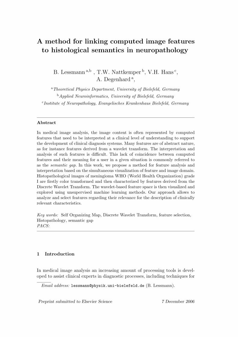
A method for linking computed image features

to histological semantics in neuropathology

B. Lessmann a,b , T.W. Nattkemper b, V.H. Hans c,A. Degenhard a,

aTheoretical Physics Department, University of Bielefeld, GermanybApplied Neuroinformatics, University of Bielefeld, Germany

cInstitute of Neuropathology, Evangelisches Krankenhaus Bielefeld, Germany

Abstract

In medical image analysis, the image content is often represented by computedfeatures that need to be interpreted at a clinical level of understanding to supportthe development of clinical diagnosis systems. Many features are of abstract nature,as for instance features derived from a wavelet transform. The interpretation andanalysis of such features is difficult. This lack of coincidence between computedfeatures and their meaning for a user in a given situation is commonly referred toas the semantic gap. In this work, we propose a method for feature analysis andinterpretation based on the simultaneous visualization of feature and image domain.Histopathological images of meningioma WHO (World Health Organization) gradeI are firstly color transformed and then characterized by features derived from theDiscrete Wavelet Transform. The wavelet-based feature space is then visualized andexplored using unsupervised machine learning methods. Our approach allows toanalyze and select features regarding their relevance for the description of clinicallyrelevant characteristics.

Key words: Self Organizing Map, Discrete Wavelet Transform, feature selection,Histopathology, semantic gapPACS:

1 Introduction

In medical image analysis an increasing amount of processing tools is devel-oped to assist clinical experts in diagnostic processes, including techniques for

Email address: lessmann@physik.uni-bielefeld.de (B. Lessmann).

Preprint submitted to Elsevier Science 7 December 2006

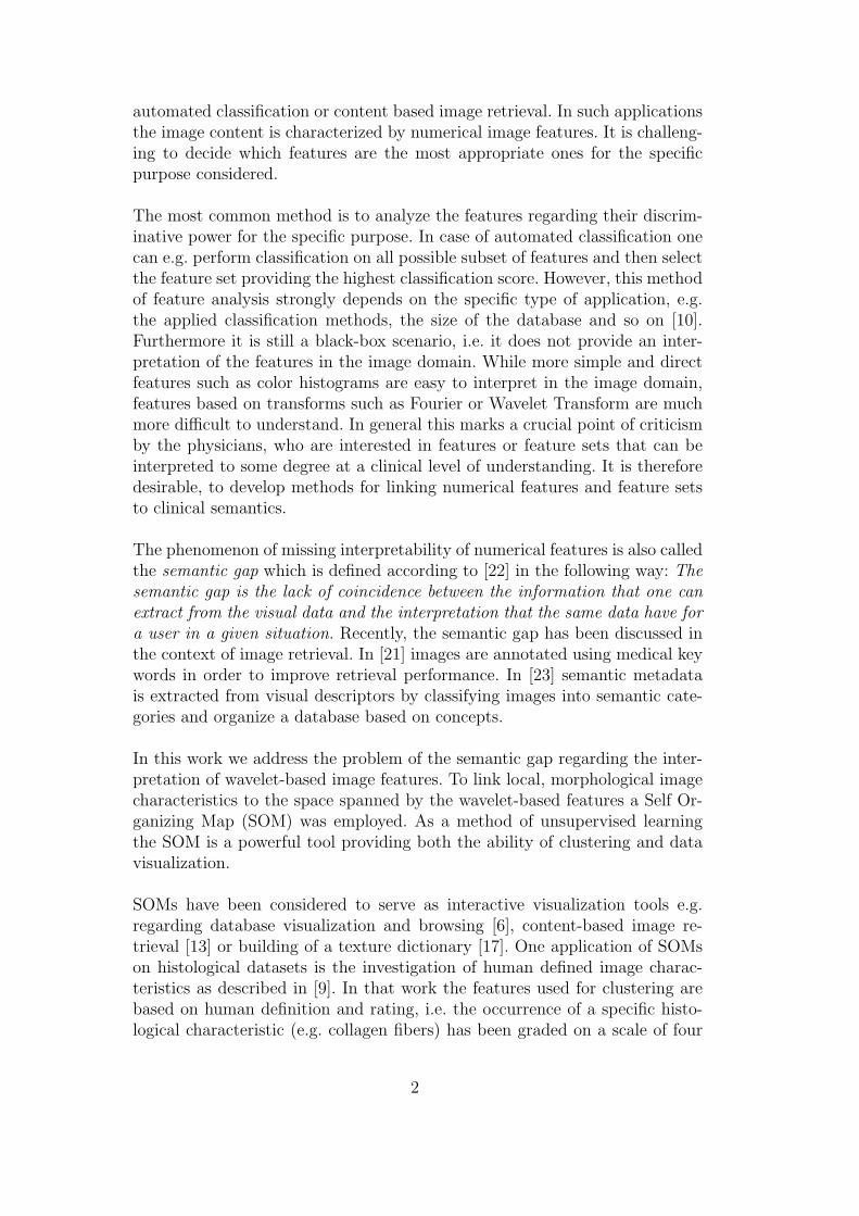
automated classification or content based image retrieval. In such applicationsthe image content is characterized by numerical image features. It is challeng-ing to decide which features are the most appropriate ones for the specificpurpose considered.

The most common method is to analyze the features regarding their discrim-inative power for the specific purpose. In case of automated classification onecan e.g. perform classification on all possible subset of features and then selectthe feature set providing the highest classification score. However, this methodof feature analysis strongly depends on the specific type of application, e.g.the applied classification methods, the size of the database and so on [10].Furthermore it is still a black-box scenario, i.e. it does not provide an inter-pretation of the features in the image domain. While more simple and directfeatures such as color histograms are easy to interpret in the image domain,features based on transforms such as Fourier or Wavelet Transform are muchmore difficult to understand. In general this marks a crucial point of criticismby the physicians, who are interested in features or feature sets that can beinterpreted to some degree at a clinical level of understanding. It is thereforedesirable, to develop methods for linking numerical features and feature setsto clinical semantics.

The phenomenon of missing interpretability of numerical features is also calledthe semantic gap which is defined according to [22] in the following way: Thesemantic gap is the lack of coincidence between the information that one canextract from the visual data and the interpretation that the same data have fora user in a given situation. Recently, the semantic gap has been discussed inthe context of image retrieval. In [21] images are annotated using medical keywords in order to improve retrieval performance. In [23] semantic metadatais extracted from visual descriptors by classifying images into semantic cate-gories and organize a database based on concepts.

In this work we address the problem of the semantic gap regarding the inter-pretation of wavelet-based image features. To link local, morphological imagecharacteristics to the space spanned by the wavelet-based features a Self Or-ganizing Map (SOM) was employed. As a method of unsupervised learningthe SOM is a powerful tool providing both the ability of clustering and datavisualization.

SOMs have been considered to serve as interactive visualization tools e.g.regarding database visualization and browsing [6], content-based image re-trieval [13] or building of a texture dictionary [17]. One application of SOMson histological datasets is the investigation of human defined image charac-teristics as described in [9]. In that work the features used for clustering arebased on human definition and rating, i.e. the occurrence of a specific histo-logical characteristic (e.g. collagen fibers) has been graded on a scale of four

2

by a human observer.

Here, we demonstrate the ability of SOMs to serve as an interface for the anal-ysis of numerical features. We demonstrate the method utilizing an exampledatabase of microscopic images of benign brain tumors. The database con-tains histopathological images of four subtypes of meningiomas. The subtypesare classified by a medical expert into four meningioma classes depending ontextural characteristics at different scales. Therefore we have chosen from thevariety of methods for texture characterization the Discrete Wavelet Trans-form as a method which allows to encode scale-dependent image information.

The SOM-based visualization of the feature space then enables us to establisha correlation between single features and histologically relevant image struc-tures and thus the selection of a subset of clinically important features.

Preliminary experiments have already been described in [14] which sufferedfrom a lack of interpretability. Utilizing a new color transform we can nowshow, how our approach can be used to bridge the gap between numericalfeatures and histopathological terms and thus transfer clinical terms into thefeature space.

2 Materials

In order to provide a test set of data for our system, we have chosen fourhistopathologically well defined subtypes of meningioma, a benign tumor ofthe coverings of the brain, i.e. the meninges [16]. The four subtypes are charac-terized by distinct features (Table 1) allowing a trained investigator to makean unequivocal diagnosis in most cases. Examples of subimages (256 × 256pixel) are shown in Figure 1. However, intermediate features are especiallycommon between fibroblastic, transitional and psammomatous subtypes.

Diagnostic tumor samples were derived from neurosurgical resections at theBethel Department of Neurosurgery, Bielefeld, Germany for therapeutic pur-poses, routinely processed for formalin fixation and paraffin embedded. Fourµm thick microtome sections were dewaxed on glass slides, stained with Mayer’shaemalaun and eosin, dehydrated, and coverslipped with mouting medium(Eukitt R©, O. Kindler GmbH, Freiburg, Germany). Archive cases from theyears 2004 and 2005 were selected for representing typical features of eachmeningioma subtype. Slides were analyzed on a Zeiss Axioskop 2 plus mi-croscope with a Zeiss Achroplan 40x/0,65 lens. After manually focusing andautomated background correction, 1300× 1030 pixels, 24 bit, true color RGBpictures were taken at standardized 3200 K light temperature in TIF formatusing Zeiss AxioVision 3.1 software and a Zeiss AxioCam HRc digital color

3

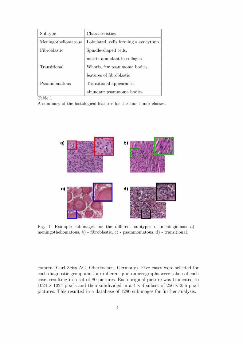
Subtype Characteristics

Meningotheliomatous Lobulated, cells forming a syncytium

Fibroblastic Spindle-shaped cells,

matrix abundant in collagen

Transitional Whorls, few psammoma bodies,

features of fibroblastic

Psammomatous Transitional appearance,

abundant psammoma bodiesTable 1A summary of the histological features for the four tumor classes.

Fig. 1. Example subimages for the different subtypes of meningiomas: a) -meningotheliomatous, b) - fibroblastic, c) - psammomatous, d) - transitional.

camera (Carl Zeiss AG, Oberkochen, Germany). Five cases were selected foreach diagnostic group and four different photomicrographs were taken of eachcase, resulting in a set of 80 pictures. Each original picture was truncated to1024 × 1024 pixels and then subdivided in a 4 × 4 subset of 256 × 256 pixelpictures. This resulted in a database of 1280 subimages for further analysis.

4

3 Methods

3.1 Color channels

In many applications RGB (Red, Green, Blue) images are transformed into acolor space more suitable for human perception, i.e. the HSV (Hue, Saturation,Value) color space [11] or the L*u*v color space [5]. Since pathology imagesare limited regarding their colors we transform the RGB values in order toenhance special image structures. In the following, we have computed twotransformed images from the RGB values (R(x,y), G(x,y), B(x,y)). Firstly,an intensity value is computed by averaging the three color channels for eachpixel and location (x, y) according to

h1(x, y) =1

3∗ [R(x, y) + G(x, y) + B(x, y)]. (1)

The images computed according to equation (1) will further be denoted asintensity images. Secondly, a transform in color space is designed to extractthe cell nuclei from the image, since they appear to exhibit significant char-acteristics for distinguishing the tumor classes. However, the image color ofa single stained tumor section inevitably depends to some extent on changesduring the preparation. To reduce dependence on these color changes, we ap-ply a mean shift to all images and color channels. The average color, in thefollowing indexed by av, is supposed to be very close to the color of thosestructures providing the largest areas in the image, in this case the cytoplasmor the psammoma bodies.

Rshift(x, y) = R(x, y)− Rav (2)

Gshift(x, y) = G(x, y)−Gav (3)

Bshift(x, y) = B(x, y)− Bav (4)

The preparation procedure described above using the routine H&E stain leadsto a blue coloration of the cell nuclei in contrast to the surrounding cytoplasmusually showing a pink color. We point out that this holds for the datasetanalyzed since it contains only WHO grade I meningioma. Some other typesof meningioma, e.g. the clear cell meningioma (WHO grade II) provide a col-oring different from the one described.After applying the mean shift to the color channels, those image structures,which are “bluer” than the surrounding tissue, are characterized by Bshift(x, y) >Rshift(x, y).

By computing

5

h1

h2

h1

h2

h2

h1

h1

h2

a) b)

c) d)

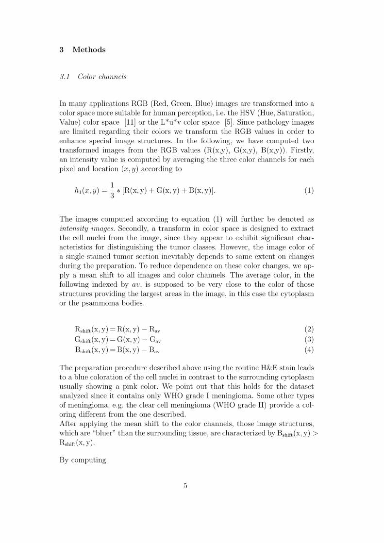
Fig. 2. Example subimages for the transform in color space. Each of the subimagesalready shown above is displayed as intensity image h1 and with enhanced cell nucleih2: a) - meningotheliomatous, b) - fibroblastic, c) - psammomatous, d) - transitional.

h2(x, y) = (maxRBshift(x, y)− Rshift(x, y)) ∗ S (5)

with maxRBshift(x, y) =max{Rshift(x, y),Bshift(x, y)} (6)

all image structures with Bshift(x, y) < Rshift(x, y) are set to zero. The remain-ing structures, which are supposed to be mainly cell nuclei, are retained.

The factor S is the saturation as defined in the HSV color space [7]

S =maxRGB(x, y)−minRGB(x, y)

maxRGB(x, y)(7)

with maxRGB(x, y) =max{R(x, y),G(x, y),B(x, y)}. (8)

This factor suppresses artefacts occurring from the white areas in the images.Especially in psammomatous meningiomas the white areas are due to artificialcracks during tissue processing and do not represent relevant staining proper-ties of the tumors. The resulting images of the transform h2 will be denotedas cell nuclei images in the further description. Figure 2 shows examples ofthe transform.

3.2 Discrete Wavelet Transform

In this work, wavelet based features are used for tissue characterization. Waveletbased multiresolution analysis enables to assess the scale-dependent informa-

6

tion in signals and images [19]. A signal f is decomposed using the Discrete(Dyadic) Wavelet Transform into a basis of shifted and dilated versions of abasic wavelet or mother wavelet ψ [4]

f(x) =∑(j,k)

dj,kψj,k(x) , (9)

with ψj,k(x) = 2j/2ψ(2jx− k) . (10)

Here the index j indicates the dilation or scaling step while k refers to trans-lation or shifting. The wavelet coefficients dj(k) are given by the scalar prod-uct dj(k) = 〈f(x), ψj,k(x)〉 or dj(k) = 〈f(x), ψ̃j,k(x)〉 in case of biorthogonalwavelets with the dual wavelet ψ̃ [4]. An efficient calculation of these coeffi-cients is accomplished by the Fast Wavelet Transform (FWT), an algorithmallowing the coefficients to be calculated in a stepwise manner. On the firstscale the signal is decomposed into its details and the remaining signal, i.e. theapproximation, reflecting the particular scale. The details are described by thewavelet coefficients of this scale while the approximation is represented by thescaling function coefficients. The procedure can be iterated by a further de-composition of the approximation into details and approximation of the nextcoarser scale [18].

In two dimensions, the wavelets are product functions of the one-dimensionalwavelet- and scaling-function. We have chosen to use the decomposition pro-cedure, which is called Nonstandard-Decomposition in [24]. The correspondingcoefficients dj,o(kx, ky) therefore do not only reflect a particular scale j, but alsoa particular orientation o in the images. The two-dimensional wavelet func-tions to be considered are ψ(x)φ(y), φ(x)ψ(y), ψ(x)ψ(y) and φ(x)φ(y). Thecoefficients corresponding to the latter one are the two-dimensional scalingfunction coefficients, further decomposed in the next step, while the coeffi-cients corresponding to the first functions provide the details in horizontal (x)direction, vertical (y) direction and the diagonal details.

3.2.1 Wavelet-based image features

Texture is probably the most important descriptor for tissue characterizationin medical textbooks. Several different texture features have been evaluatedin literature, including e.g. co-occurrence matrices, line-angle-ratio statistics[1,8], Gabor filters [8] or wavelet based features [26]. A comprehensive overviewof texture features can be found in [20]. In this work the texture characteri-zation does not involve a prior segmentation as e.g. in [5] but is performed onthe entire subimages. To access the scale-dependent information we decidedto use multiresolution wavelet features, as calculated by the discrete wavelettransform. We use a pair of symmetric, biorthogonal wavelets, developed by

7

Cohen, Daubechies and Feauveau. These pairs of scaling and wavelet-functionsare indicated as φ2, φ̃2,2, ψ2,2, ψ̃2,2 in [3]. As described in [2] and [25] the l1 orl2-norm of the detail coefficients corresponding to one scale and orientationcan be used as powerful texture features. In this work the l1-norm, i.e. themean absolute coefficient (MAC) of each scale and orientation has been com-puted according to l1(dj,o) =

∑kx,ky

|dj,o(kx, ky)|. The final feature vectors arebased on these MACs. As shown in [14] two types of features based on theseMACs were found to be appropriate to characterize the four types of tissue.Firstly, a mean absolute coefficient for each scale j is computed according to

f1(j) =∑o

MAC(o, j), j = 1..8, o = o1, o2, o3. (11)

Again j is the scale index, while index o indicates the orientation in the image.The indices o1 and o2 indicate coefficients in vertical or horizontal direction,while o3 indicates the diagonal details.

Secondly, we use a feature set f2 describing whether the image structures areanisotropic, i.e. orientated in a preferred orientation.

f2(j) = |MAC(o1, j)−MAC(o2, j)|+ c MAC(o3, j), j = 1..8 (12)

In case of image structures mainly orientated in horizontal or vertical direc-tion, either the MAC for o1 or o2 should be significantly increased, while theother one is correspondingly decreased. Therefore |MAC(o1, j)−MAC(o2, j)|reaches a high value. Regarding image structures orientated in a diagonal di-rection the first part of equation (12) vanishes, but, at the same time, the sec-ond part increases. The normalization factor c assures that the added MACshave equalized variances such that the influences of both parts of the sum arecomparable. In contrast to [14] each component of the second feature set isnot normalized to the corresponding component of the first set. We point out,that a similar approach to characterize images by scale- and orientation-relatedtexture measures using wavelets has already used for the characterization ofcorrosion images [15]. However, there the computed features used differ fromthe ones we computed in this work.

3.3 Self Organizing Map

The Self Organizing Map (SOM) is a clustering approach from the field of ar-tificial neural networks [12]. A set of reference or prototype vectors {uj},uj ∈Rn, is trained according to a given data set of feature vectors {xi},xi ∈Rn. Here, n is the number of features. The SOM is represented by a two-

8

dimensional square grid, which consists of nodes each associated to one ofthe reference vectors. During each learning step t a vector from the inputspace xk is selected and the nearest reference vector um (winner node) isidentified by |um − xk| = minj|uj − xk| . The nodes are updated accord-ing to uj(t + 1) = uj(t) + hmj(t)[xk − uj(t)]. The function hmj is defined as

hmj = α(t) exp− |rm−rj |22σ2(t)

, where α(t) is the learning rate factor. The vectorsrm and rj are the coordinates of the nodes in the SOM grid, with the winnernode m. The function σ(t) also decreases with time in order to reduce theneighborhood included in the training procedure with time. The decreasing ofboth functions freezes the SOM after a given number of iterations [12]. After asuccessful training procedure the reference vectors depict the data distributionin the data set preserving the topology.

3.3.1 SOM-based exploration procedure

The SOM is applied to visualize and explore a database content based onspecific image features. Since the images have a size of 256×256 pixels, featuresof eight scales can be computed. The features of the coarsest two scales areneglected, since the associated coefficients encode details corresponding to thetotal or a quarter image, which does not seem to be senseful. Considering thetwo sets of features (f1, f2), the two color channels (h1, h2) described aboveand the remaining six scales a total number of 24 possible features has to betaken into account.

The training procedure has been accomplished two times, firstly using the firstset of features f1 (12 feature vector components), secondly using the secondset of features f2 (12 feature vector components). The results are shown inthe Figures 3 and 4 respectively. An 8× 8 SOM grid has been utilized for theexploration procedure. In each figure three types of SOM visualizations arepresented. At the top the clustering result is shown. For each feature vector,i.e. each subimage, the nearest reference vector of the trained SOM can becomputed. In this way, each subimage is mapped to one node in the SOMgrid. In the visualization at the top each subimage is symbolized by a pointof the color corresponding to the class of tissue. This point is displayed atthe specific node, thus each node is visualized by the corresponding clusterof feature vectors mapped to this node. In the middle the same SOM gridis visualized in another mode. Here each node is marked with one of thesubimages of the respective cluster. To be explicit, the subimage associatedwith the nearest feature vector has been chosen from the dominating tumorclass at the specific node. In this way, the distribution of histological featurescan be explored. At the bottom of the figure the Component Plane Mapsare shown, a special visualization of the reference vector components. Eachlittle square is a visualization of the SOM grid and one component of thereference vectors. The gray value shows the distribution of this component on

9

the SOM grid. Since the reference vectors have twelve components in bothcases, twelve Component Plane Maps are shown, one map for each componentof the reference vector. Black color symbolizes low values of the component,white color indicates high values.

3.3.1.1 Feature set f1 Starting with the analysis of Figure 3, the fol-lowing conclusions can be derived. The clustering results visualized at thetop shows that this set of features is appropriate to discriminate psammoma-tous (blue) and transitional (black) images. However, the meningothelioma-tous (red) and the fibroblastic (green) classes are still strongly mixed. This isespecially due to the feature vector components 1− 6, which are the featuresof the intensity image h1. In the Component Plane Maps these componentsvary strongly from the top to the bottom of the SOM grid. By exploring thecorresponding subimages it becomes clear, that these components are linkedto tissue inhomogeneities in the extracellular matrix, which occur in bothclasses. Furthermore the high scale component (component six) additionallyintroduces an inner-class separation in the psammomatous group of tissue(from top right to bottom right). The visualization of histological character-istics reveals that this component is especially high in those images showinglarge cracks in the tissue (bottom right of the SOM grid). Since the amount ofcracks in the tissue varies strongly in psammomatous tissue it is not consideredto be of diagnostic relevance. We will therefore neglect the components 1− 6of feature set f1. The visualization further reveals some redundancy in thecomponents 7− 12 of this feature set. These components show a very similardistribution. Some of them can therefore also be neglected. From the featureset f1 only the components 9−10 are chosen for tissue characterization. Thesecomponents correspond to the scales 3 and 4 of the cell nuclei image h2.

3.3.1.2 Feature set f2 As described above this set of features is con-structed to describe preferred orientations in the image. As expected the sep-aration of the fibroblastic and the meningotheliomatous class as visualizedat the top of the figure is significantly increased compared to feature set f1.However, the Component Plane Maps reveal that the components 6 and 12 as-sociated to very coarse scale details do not show a distribution correspondingto some histological interpretation and are therefore neglected. The remain-ing components show strong redundancy, so in a next step we only choosethe components 3, 4, 9, 10 for tissue characterization. These components cor-respond to the scales three and four of both color channels h1 and h2. The sixselected features are summarized in table 2.

10

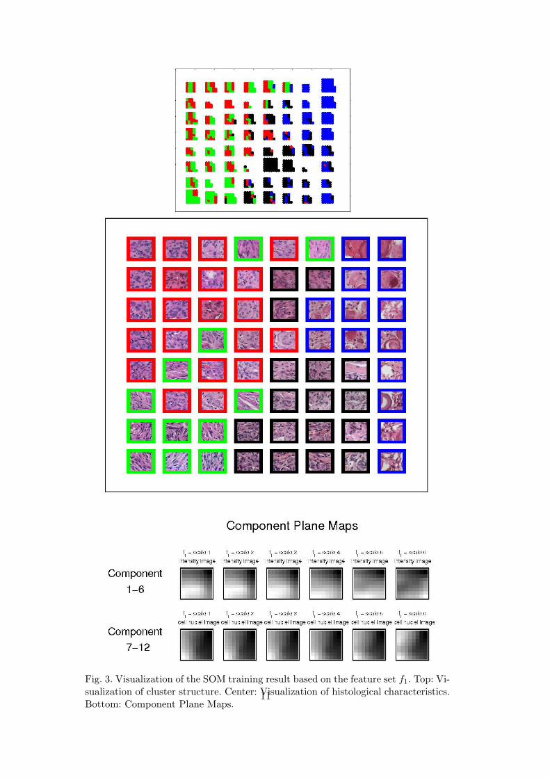
Fig. 3. Visualization of the SOM training result based on the feature set f1. Top: Vi-sualization of cluster structure. Center: Visualization of histological characteristics.Bottom: Component Plane Maps.

11

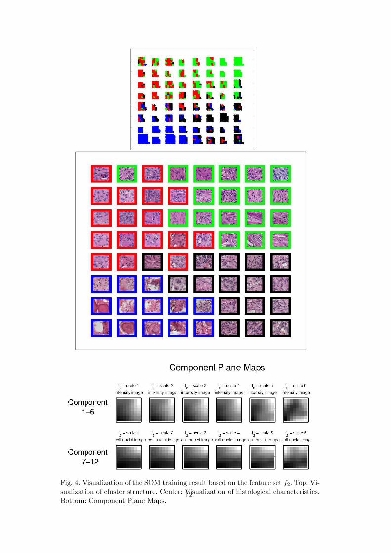
Fig. 4. Visualization of the SOM training result based on the feature set f2. Top: Vi-sualization of cluster structure. Center: Visualization of histological characteristics.Bottom: Component Plane Maps.

12

set of features h1 h2

f1 scale 3 & 4

f2 scale 3 & 4 scale 3 & 4Table 2Final set of features employed for tissue characterization.

4 Results and Discussion

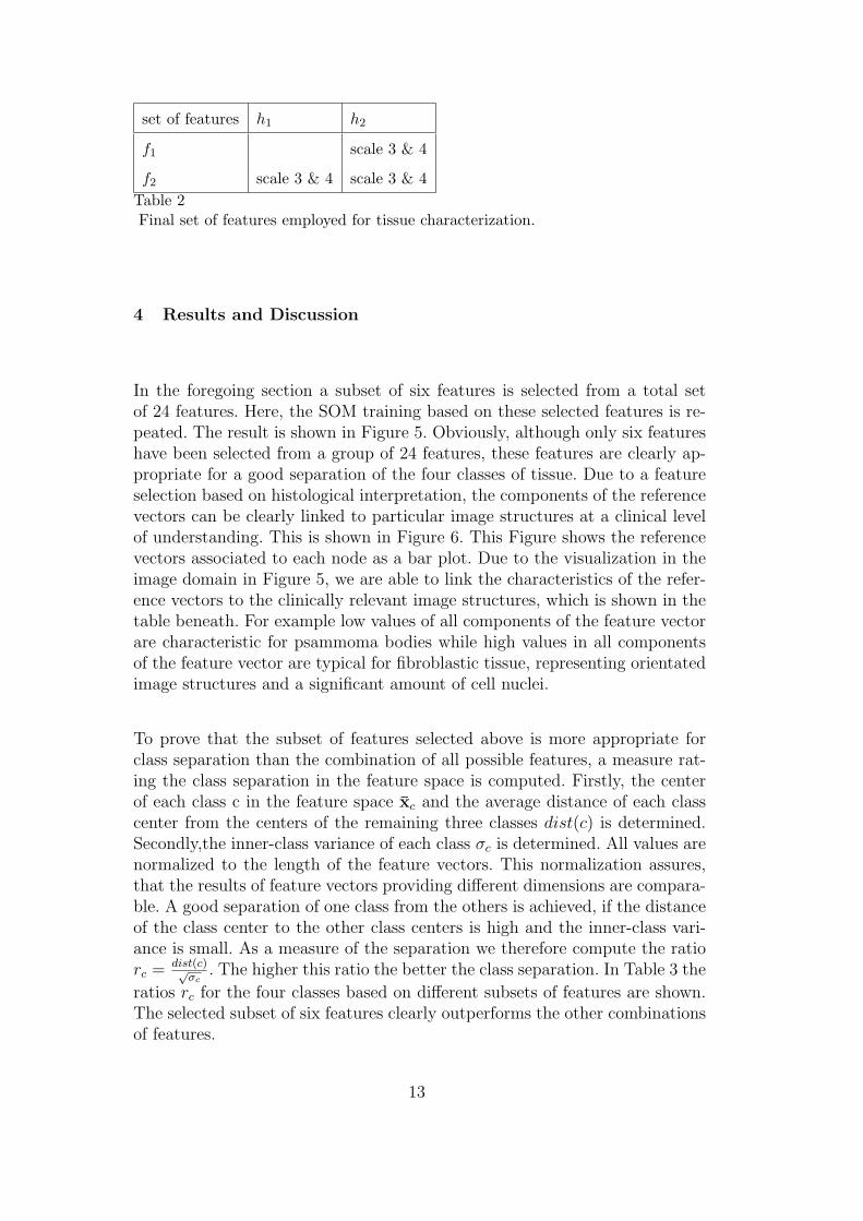
In the foregoing section a subset of six features is selected from a total setof 24 features. Here, the SOM training based on these selected features is re-peated. The result is shown in Figure 5. Obviously, although only six featureshave been selected from a group of 24 features, these features are clearly ap-propriate for a good separation of the four classes of tissue. Due to a featureselection based on histological interpretation, the components of the referencevectors can be clearly linked to particular image structures at a clinical levelof understanding. This is shown in Figure 6. This Figure shows the referencevectors associated to each node as a bar plot. Due to the visualization in theimage domain in Figure 5, we are able to link the characteristics of the refer-ence vectors to the clinically relevant image structures, which is shown in thetable beneath. For example low values of all components of the feature vectorare characteristic for psammoma bodies while high values in all componentsof the feature vector are typical for fibroblastic tissue, representing orientatedimage structures and a significant amount of cell nuclei.

To prove that the subset of features selected above is more appropriate forclass separation than the combination of all possible features, a measure rat-ing the class separation in the feature space is computed. Firstly, the centerof each class c in the feature space x̄c and the average distance of each classcenter from the centers of the remaining three classes dist(c) is determined.Secondly,the inner-class variance of each class σc is determined. All values arenormalized to the length of the feature vectors. This normalization assures,that the results of feature vectors providing different dimensions are compara-ble. A good separation of one class from the others is achieved, if the distanceof the class center to the other class centers is high and the inner-class vari-ance is small. As a measure of the separation we therefore compute the ratiorc = dist(c)√

σc. The higher this ratio the better the class separation. In Table 3 the

ratios rc for the four classes based on different subsets of features are shown.The selected subset of six features clearly outperforms the other combinationsof features.

13

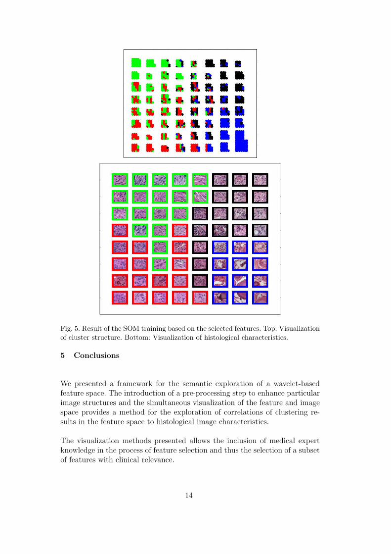
Fig. 5. Result of the SOM training based on the selected features. Top: Visualizationof cluster structure. Bottom: Visualization of histological characteristics.

5 Conclusions

We presented a framework for the semantic exploration of a wavelet-basedfeature space. The introduction of a pre-processing step to enhance particularimage structures and the simultaneous visualization of the feature and imagespace provides a method for the exploration of correlations of clustering re-sults in the feature space to histological image characteristics.

The visualization methods presented allows the inclusion of medical expertknowledge in the process of feature selection and thus the selection of a subsetof features with clinical relevance.

14

orientatedamount ofincreasing

structures

1 6 1 6 1 6 1 6 1 6 1 6 1 6 1 6

fascicular structure

bodies

collagen rich areas

increasing number of cell nuclei

spindle−shaped cell nuclei

psammoma

Component histological interpretation

1+2 number of cell nuclei

especially low values in psammoma bodies and areas of collagen

3+4 Amount of anisotropic tissue inhomogeneities

especially high values in case of parallel aligned cracks

in fibroblastic tissue

5+6 Anisotropic shaped cell nuclei

especially high values in fibroblastic tissue

Fig. 6. Top: A histological feature map derived from the visualization procedure. TheMap allows to clearly link numerical features to histological semantics (Bottom).

Due to selection of a small subset of features computational costs are re-duced and difficulties associated with large feature vectors, sometimes calledthe curse of dimensionality [10] can be avoided. Additionally, by utilizing aclass separation measure it was proven that the selected subset of featuresleads to a separation of the four classes in the feature space with highestaccuracy.

15

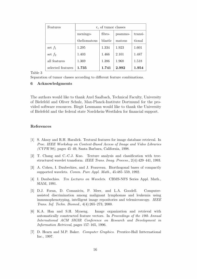
Features rc of tumor classes

meningo- fibro- psammo- transi-

theliomatous blastic matous tional

set f1 1.295 1.334 1.923 1.601

set f2 1.403 1.466 2.101 1.487

all features 1.369 1.386 1.968 1.518

selected features 1.735 1.741 2.992 1.954Table 3Separation of tumor classes according to different feature combinations.

6 Acknowledgments

The authors would like to thank Axel Saalbach, Technical Faculty, Universityof Bielefeld and Oliver Schulz, Max-Planck-Institute Dortmund for the pro-vided software resources. Birgit Lessmann would like to thank the Universityof Bielefeld and the federal state Nordrhein-Westfalen for financial support.

References

[1] S. Aksoy and R.H. Haralick. Textural features for image database retrieval. InProc. IEEE Workshop on Content-Based Access of Image and Video Libraries(CVPR’98), pages 45–49, Santa Barbara, California, 1998.

[2] T. Chang and C.-C.J. Kuo. Texture analysis and classification with tree-structured wavelet transform. IEEE Trans. Imag. Process., 2(4):429–441, 1993.

[3] A. Cohen, I. Daubechies, and J. Feauveau. Biorthogonal bases of compactlysupported wavelets. Comm. Pure Appl. Math., 45:485–559, 1992.

[4] I. Daubechies. Ten Lectures on Wavelets. CBMS-NFS Series Appl. Math.,SIAM, 1991.

[5] D.J. Foran, D. Comaniciu, P. Meer, and L.A. Goodell. Computer-assisted discrimination among malignant lymphomas and leukemia usingimmunophenotyping, intelligent image repositories and telemicroscopy. IEEETrans. Inf. Techn. Biomed., 4(4):265–273, 2000.

[6] K.A. Han and S.H. Myaeng. Image organization and retrieval withautomatically constructed feature vectors. In Proceedings of the 19th AnnualInternational ACM SIGIR Conference on Research and Development inInformation Retrieval, pages 157–165, 1996.

[7] D. Hearn and M.P. Baker. Computer Graphics. Prentice-Hall IntternationalInc., 1997.

16

[8] P. Howarth, A. Yavlinsky, D. Heesch, and S. Rueger. Medical image retrievalusing texture, locality and colour. In C. Peters, P. Clough, and J. Gonzalo,editors, 5th Workshop of the Cross-Language Evaluation Forum, CLEF 2004,Bath, UK, Lecture Notes in Computer Science, pages 740–749. Springer, 2004.

[9] J.R. Iglesias-Rozas and N. Hopf. Histological heterogeneity of humanglioblastomas investigated with an unsupervised neural network (SOM).Histology and Histopathology, 20:351–356, 2005.

[10] A.K. Jain, R.P.W. Duin, and J. Mao. Statistical pattern recognition: A review.IEEE Trans. Patt. Anal. Machine Intell., 22(1):4–37, 2000.

[11] J. Jelonek, K. Krawiec, R. Slowinski, and J. Szymas. Intelligent decision supportin pathomorphology. Pol. J. Pathol., 50(2):115–118, 1999.

[12] T. Kohonen. Self Organizing Maps. Springer, Berlin, Heidelberg, 1995.

[13] J. Laaksonen, M. Koskela, Sami Laakso, and Erkki Oja. Picsom - content-based image retrieval with self-organizing maps. Pattern Recognition Letters,22:1199–1207, 2000.

[14] B. Lessmann, V. Hans, A. Degenhard, and T.W. Nattkemper. Feature-spaceexploration of pathology images using content-based database visualization.In J.M. Reinhardt and J.P.W. Pluim, editors, Proceedings of SPIE MedicalImaging, volume 6144, 61445Z, San Diego, California, USA, 2006.

[15] S. Livens, P. Scheunders, G. van de Wouwer, D. van Dyck, H. Smets,J. Winkelmans, and W. Bogaerts. A texture analysis approach to corrosionimage classification. Microscopy, Microanalysis, Microstructures, 7(2):1–10,1996.

[16] DN. Louis, B.W. Scheithauer, H. Budka, A. von Deimling, and J.J. Kepes.Meningiomas. In P. Kleihues and W.K.Cavenee, editors, World HealthOrganization Classification of Tumours. Pathology & Genetics. Tumours of theNervous System., pages 176–184. IARC Press, Lyon, 2000.

[17] W. Y. Ma and B. S. Manjunath. Image indexing using a texture dictionary. InSPIE conference on Image Storage and Archiving System, volume 2606, pages288–298, 1995.

[18] S. Mallat. A Wavelet Tour of Signal Processing. Academic Press, San Diego,London, 1999.

[19] S. Mallat and S. Zhong. Characterization of signals from multiscale edges. IEEETrans. Patt. Anal. Machine Intell., 14:710–723, 1992.

[20] B.S. Manjunath and W.Y. Ma. Texture features for image retrieval. InV. Castelli and L.D. Bergman, editors, Image Databases - Search and Retrievalof Digital Imagery. John Wiley and Sons, Inc, New York, 2002.

[21] H. Mueller, P. Ruch, and A. Geissbuhler. Enriching content-based imageretrieval with automatically extracted mesh terms. In GMDS conference, pages266–269, Innsbruck, Austria, 2004.

17

[22] A.W. Smeulders, M. Worring, S. Santini, A. Gupta, and R. Jain. Content-basedimage retrieval systems at the end of the early years. IEEE Trans. Patt. Anal.Machine Intell., 22(12):1349–1380, 2000.

[23] J. Stauder, J. Sirot, H. Le Borgne, E. Cooke, and N. E. O’Connor. Relatingvisual and semantic image descriptors. In Proc. European Workshop for theIntegration of Knowledge, Semantics and Digital Media Technology (EWIMT),London, 2004.

[24] E.J. Stollnitz, T.D. Derose, and D.H. Salesin. Wavelets for Computer Graphics.Morgan Kaufmann Publishers, San Francisco, 1996.

[25] G. van de Wouwer, P. Scheunders, and D. van Dyck. Statistical texturecharacterization from discrete wavelet representation. IEEE Trans. Imag. Proc.,8(4):592–598, 1999.

[26] G. van de Wouwer, B. Weyn, P. Scheunders, W. Jacob, E. van Marck, andD. van Dyck. Wavelets as chromatin texture descriptors for the automatedidentification of neoplastic nuclei. J. Microscopy, 197:25–35, 1999.

18