An Interactive Intelligent Decision Support System for ...

An Interactive Intelligent Decision Support System for Integration of Inventory,

Planning, Scheduling and Revenue Management

A dissertation presented to

the faculty of

the Russ College of Engineering and Technology of Ohio University

In partial fulfillment

of the requirements for the degree

Doctor of Philosophy

Ehsan Ardjmand

August 2015

© 2015 Ehsan Ardjmand. All Rights Reserved.

2

This dissertation titled

An Interactive Intelligent Decision Support System for Integration of Inventory,

Planning, Scheduling and Revenue Management

by

EHSAN ARDJMAND

has been approved for

the Department of Industrial and Systems Engineering

and the Russ College of Engineering and Technology by

Gary R. Weckman

Associate Professor of Industrial and Systems Engineering

Dennis Irwin

Dean, Russ College of Engineering and Technology

3

ABSTRACT

ARDJMAND, EHSAN, Ph.D., August 2015, Mechanical and Systems Engineering

An Interactive Intelligent Decision support system for Integration of Inventory, Planning,

Scheduling and Revenue Management

Director of Dissertation: Gary R. Weckman

The long-term permanency and profitability of a firm requires decisions to be

made wisely and on time. For this purpose, it is essential to consider all aspects of a

decision in terms of its impact on revenue, planning, scheduling, and inventory in an

integrated framework.

In this research paper, an interactive intelligent decision support system for

making an integrated decision in the presence of demand uncertainty is proposed. The

system operates in a multi-product, multi-period setting, and its objective is to maximize

the profit of the firm over time. To achieve its objective, the system first obtains the

optimal price and capacity plan for the coming periods. The output of this first step

becomes the input for the second step, in which the problem of scheduling is solved. At

the end, based on the scheduling step, the optimum inventory policy is determined.

To cope with demand uncertainty in the pricing and planning phase, a robust

optimization model is proposed in which the demand is considered to belong to an

interval and there is no knowledge (such as statistical distribution) associated with the

demand. The robust problem is solved using a metaheuristic.

During the scheduling step, a general setting for the problem is considered, in

which each product is treated like a project with a flow network. To address the problem

4 of scheduling, a simulation optimization method is applied in which the optimization step

determines the dispatch rule of the jobs and the simulation step schedules the dispatched

jobs on the production line.

During the inventory step, the system obtains the best schedule for ordering and

storing the raw material in order to minimize the inventory cost. For this purpose, a

mixed integer mathematical model is proposed and a metaheuristic is applied to obtain

the best solution.

All modules of the proposed decision support system are supported with a

database that stores the data obtained from the shop floor and the market. This database is

used to assess the costs and parameters in models by applying a cost estimation support

system.

To evaluate the effectiveness of the proposed decision support system, it has

implemented in a small size textile production line. The data generated by the system and

its users are analyzed for a period of four months. Four indicators of profit per product,

overall equipment effectiveness, percentage of realized schedule and work-in-progress

are monitored during these four months and their values are compared against the same

time period in previous year. The results show that the system has improved in terms of

profitability, equipment effectiveness and production line control. However, the work-in-

progress has not improved.

5

DEDICATION

To my parents and wife, Fereydoon, Tayebeh and Maria

6

ACKNOWLEDGMENTS

First, I would like to express my sincere gratitude to my advisor Dr. Gary R.

Weckman who helped me greatly in the course of this research. Had it not been for his

confidence in me and invaluable guidance that gone far beyond this dissertation, my

academic life would have not been possible. I owe him a great many thanks for his

support and friendship.

My deepest thanks to Dr. William A. Young for providing me the opportunity to

broaden my academic perspective by teaching and involve me in various research

projects. His enthusiasm, encouragement, and faith in me have been extremely

contributed to this dissertation.

I would also like to thank Dr. Namkyu Park for his brilliant comments and

intellectual support. He was always available for my questions and knew where to look

for the answers while leading me to the right direction in both theory and practice.

My sincere thanks go to my dissertation committee Dr. Andy Snow and Dr.

Hajrudin Pasic for their thoughtful feedback, which has added value to this research.

Special thanks to Bradly Weckman for his great comments on the manuscript and Dr.

Weckman’s lovely wife, Janet that always supported me spiritually.

7

TABLE OF CONTENTS

Page

Abstract ............................................................................................................................... 3

Dedication ........................................................................................................................... 5

Acknowledgments............................................................................................................... 6

List of Tables .................................................................................................................... 12

List of Figures ................................................................................................................... 14

1 Introduction ............................................................................................................... 18

1.1 Background ....................................................................................................... 19

1.2 Problem ............................................................................................................. 21

1.3 Significance....................................................................................................... 22

1.4 Implementation and Data Acquisition .............................................................. 22

2 Literature Review ...................................................................................................... 23

2.1 Decision Support Systems (DSS) ..................................................................... 23

2.2 Pricing and Revenue Management Systems ..................................................... 28

2.3 Forecasting Support Systems ............................................................................ 31

2.4 Cost Estimation Decision Support Systems ...................................................... 38

2.5 Planning and Scheduling Support Systems....................................................... 41

2.6 Inventory Management Systems ....................................................................... 50

2.7 Limitations ........................................................................................................ 55

3 General Framework of the System ........................................................................... 57

3.1 Cost Estimation ................................................................................................. 58

8

3.2 Pricing and Planning ......................................................................................... 58

3.3 Scheduling......................................................................................................... 59

3.4 Inventory ........................................................................................................... 59

4 Financial and Cost Estimation Module ..................................................................... 60

4.1 Inputs................................................................................................................. 60

4.1.1 Cost Centers ............................................................................................................. 60

4.1.2 Costs ......................................................................................................................... 61

4.2 Processes ........................................................................................................... 62

4.2.1 Estimating Finished Costs ........................................................................................ 62

4.2.2 Estimating Inventory Costs ...................................................................................... 63

4.2.3 Estimating Lost Sale Cost ........................................................................................ 64

4.3 Design and Outputs of Finance and Cost Estimation Module .......................... 64

5 Pricing and Planning Module .................................................................................... 66

5.1 Inputs................................................................................................................. 66

5.1.1 Inputs from Finance and Cost Estimation Module ................................................... 67

5.1.2 Resource Constraints ................................................................................................ 67

5.1.3 Demand and Uncertainty .......................................................................................... 67

5.2 Processes ........................................................................................................... 70

5.2.1 Robust Optimization ................................................................................................ 74

5.2.2 Non-linear Model ..................................................................................................... 76

5.2.3 Linear Model ............................................................................................................ 78

5.2.4 Robust Model ........................................................................................................... 80

5.2.5 Solution Methods ..................................................................................................... 82

5.2.5.1 Exact Method ........................................................................................ 83

9

5.2.5.2 Unconscious Search .............................................................................. 83

5.2.5.3 Applying an Unconscious Search to Pricing and Planning Module ..... 94

5.2.5.4 Verification of Unconscious Search Results......................................... 96

5.3 Design and Outputs of Pricing and Planning Module ...................................... 98

6 Scheduling Module ................................................................................................. 100

6.1 Inputs............................................................................................................... 100

6.1.1 Inputs from Pricing and Planning Module ............................................................. 100

6.1.2 Timeline and Working Hours ................................................................................. 101

6.1.3 Machines ................................................................................................................ 101

6.1.4 Maintenance ........................................................................................................... 103

6.1.5 Stations ................................................................................................................... 103

6.1.6 Setup Times ............................................................................................................ 103

6.1.7 Operators and Skill Levels ..................................................................................... 104

6.1.8 Operation Chart ...................................................................................................... 104

6.2 Processes ......................................................................................................... 105

6.2.1 Scheduling .............................................................................................................. 106

6.2.1.1 Scheduling One Job ............................................................................ 109

6.2.1.2 Optimizing Dispatching Rule Using Variable Neighborhood Search 113

6.2.2 Control ................................................................................................................... 116

6.3 Design and Outputs of Scheduling Module .................................................... 118

7 Inventory Management Module .............................................................................. 120

7.1 Inputs............................................................................................................... 120

7.1.1 Inputs from Scheduling Module ............................................................................. 120

10

7.1.2 Inventory Holding Cost .......................................................................................... 121

7.1.3 Bill of Material (BOM) .......................................................................................... 121

7.1.4 Suppliers and Material Specifications .................................................................... 121

7.2 Processes ......................................................................................................... 122

7.2.1 Mathematical Model .............................................................................................. 122

7.2.2 Solution Methods ................................................................................................... 124

7.2.2.1 Exact Solution ..................................................................................... 125

7.2.2.2 Hybrid Tabu Search and Simplex Algorithm ..................................... 125

7.2.2.3 Verification of Hybrid Algorithm ....................................................... 128

7.3 Design and Outputs of Inventory Management Module ................................. 129

8 Experimentation ...................................................................................................... 131

8.1 Introducing the Textile Factory and Shop Floor ............................................. 131

8.2 Introducing the Products ................................................................................. 147

8.3 Estimating the Costs and Resource Constraints.............................................. 153

8.4 Pricing, Planning and Price of Robustness ..................................................... 155

8.5 Scheduling....................................................................................................... 163

8.6 Inventory Management ................................................................................... 166

8.7 Performance Evaluation of the System ........................................................... 173

8.7.1 Profit per Product ................................................................................................... 174

8.7.2 Overall Equipment Effectiveness (OEE) ............................................................... 176

8.7.3 Percentage of Realized Schedule ........................................................................... 177

8.7.4 Work-in-Progress (WIP) ........................................................................................ 178

9 Concluding Remarks and Future Works ................................................................. 180

11

9.1 Financial and Cost Estimation Module ........................................................... 181

9.2 Pricing and Planning Module.......................................................................... 181

9.3 Scheduling....................................................................................................... 182

9.4 Inventory Management ................................................................................... 183

9.5 Implementation ............................................................................................... 183

9.6 Limitations and Generalizability..................................................................... 184

9.7 Future Works .................................................................................................. 185

References ....................................................................................................................... 187

Appendix A: Cplex Code for Pricing and Planning Module .......................................... 222

Appendix B: Simplex Code Used in Pricing and Planning Module ............................... 227

Appendix C: Work Profile Database .............................................................................. 232

Appendix D: Machine and Maintenance Database ......................................................... 233

Appendix E: Cplex Code for Inventory Management Module ....................................... 234

12

LIST OF TABLES

Page

Table 1. DSS interaction taxonomy (Haettenschwiler, 2001) .......................................... 27

Table 2. DSS use taxonomy (D. Power, 2002) ................................................................. 27

Table 3. Categorization of pricing and revenue management systems in manufacturing

literature based on different types of DSSs............................................................... 30

Table 4. Different types of forecasting support systems designed for different forecasting

issues ......................................................................................................................... 34

Table 5. Different types of DSSs designed based on various cost estimation methods ... 40

Table 6. Different types of planning support systems designed for different scheduling

and planning problems .............................................................................................. 45

Table 7: Different types of planning support systems designed for different inventory

problems’ level.......................................................................................................... 52

Table 8: The time (hour) each product spent on each cost center and the total expenses

recorded in each cost center (CC) ............................................................................. 63

Table 9: Share of each product in each cost center and its finished cost.......................... 63

Table 10: Test problems’ specifications used for evaluation of unconscious search ....... 97

Table 11: Solution quality and run time of exact and US algorithms for six artificially

generated test problems; for each instance, US has run 10 times ............................. 98

Table 12. Six randomly generated test problems for verifying the hybrid algorithm..... 128

13 Table 13. Solution quality and run time of exact and hybrid algorithms for six artificially

generated test problems where for each instance the hybrid algorithm has run 10

times ........................................................................................................................ 129

Table 14: Price points for each product in each period, suggested by sales department 148

Table 15: The min. and max. demand for each product per price point in period 1 ...... 149




Table 19: Estimated production, inventory, and lost sale costs for products ................. 154

Table 20: Prices obtained by pricing and planning module for each period ($)............. 156

Table 21: Production plan obtained by pricing and planning module ............................ 157

Table 22: Production plan for worst-case scenario ......................................................... 161

Table 23: Chosen prices for each product in each period for the worst-case scenario ... 162

Table 24: Fabric consumption for each product (yard) .................................................. 168

Table 25: Purchasing cost of each fabric from different suppliers ................................. 169

Table 26: Consumption of each fabric in each period .................................................... 170

Table 27: Material plan for each fabric that needs to be ordered by a specific supplier in

periods 1 and 2 ........................................................................................................ 171

Table 28: Material plan for each fabric that needs to be ordered by a specific supplier in

periods 3 and 4 ........................................................................................................ 172

14

LIST OF FIGURES

Page

Figure 1. Evolution and progress of DSSs in time ........................................................... 26

Figure 2. Areas of revenue management in manufacturing ............................................. 29

Figure 3. Design, selection/specification and evaluation issues in forecasting (adopted

from (Winklhofer et al., 1996))................................................................................. 34

Figure 4. Different methods of cost estimation and their application in different stages of

product development (adopted from Duverlie and Castelain (1999)) ...................... 39

Figure 5. Complexity hierarchy of scheduling problems based on machine environments

(adopted from (Pinedo, 2012)) .................................................................................. 42

Figure 6. complexity hierarchy of scheduling problems based on processing

properties/constraints (adopted from (Pinedo, 2012)) .............................................. 43

Figure 7. complexity hierarchy of scheduling problems based on objective functions

(adopted from (Pinedo, 2012)) .................................................................................. 43

Figure 8. Information flow chart in manufacturing (adopted from (Pinedo, 2012)) ........ 45

Figure 9. General framework and modules of the proposed decision support system ..... 57

Figure 10. Relation of costs, cost types and cost centers ................................................. 61

Figure 11. Inputs, processes and outputs of finance and cost estimation modules .......... 65

Figure 12. A Schematic diagram of relation of demand and price for a specific product

and period where each bar shows the minimum and maximum of demand for

different values of price ............................................................................................ 69

Figure 13. Translation function and measurement matrix................................................ 88

15 Figure 14. Functions of and for the situation where there are two decision variables,

and .................................................................................................................. 93

Figure 15. Flow chart of applying unconscious search to pricing and planning module . 96

Figure 16. A prototype of pricing and planning interface ................................................ 99

Figure 17. Inputs, processes and outputs of the pricing and planning module ................ 99

Figure 18. The lean time remains after subtracting the repair and inefficient times plus

the amount of time a machine is producing defective products .............................. 102

Figure 19. A prototype of an operation chart consisting of six stages ........................... 105

Figure 20. General framework of the heuristic used in a scheduling module ................ 109

Figure 21. A product’s operation chart and its critical path ........................................... 110

Figure 22. a) original timeline b) timeline after scheduling task A ................................ 111

Figure 23. Flowchart of scheduling a single job ............................................................ 113

Figure 24. VNS algorithm for finding the best sequence of jobs for scheduling ........... 115

Figure 25. Schematic domain model of the database for a control process in terms of the

scheduling module .................................................................................................. 118

Figure 26. Inputs, processes and outputs of a scheduling module ................................. 119

Figure 27. Flowchart of the hybrid tabu search and Simplex algorithm applied to the

inventory management problem ............................................................................. 127

Figure 28. Input and outputs of inventory management module .................................... 130

Figure 29. The material needed and activities involved in “support” station for producing

coat 832 ................................................................................................................... 133

Figure 30. Support station standard configuration ......................................................... 134

16 Figure 31. The materials needed and activities involved in “front” station for producing

coat 832 ................................................................................................................... 135

Figure 32. Front station standard configuration ............................................................. 136

Figure 33. The materials needed and activities involved in “back” station for producing

coat 832 ................................................................................................................... 136

Figure 34. Back station standard configuration .............................................................. 137

Figure 35. The materials needed and activities involved in “sleeve” station for producing

coat 832 ................................................................................................................... 138

Figure 36. Standard configuration of sleeve station ....................................................... 138

Figure 37. The materials needed and activities involved in “hem” station for producing

coat 832 ................................................................................................................... 139

Figure 38. Standard configuration of hem station .......................................................... 139

Figure 39. The materials needed and activities involved in “lining” station for producing

coat 832 ................................................................................................................... 140

Figure 40. Standard configuration of lining station ........................................................ 141

Figure 41. The materials needed and activities involved in “collar” station for producing

coat 832 ................................................................................................................... 142

Figure 42. Standard configuration of collar station ........................................................ 142

Figure 43. The materials needed and activities involved in “body assembly” station for

producing coat 832 .................................................................................................. 143

Figure 44. Standard configuration of body assembly station ......................................... 143

17 Figure 45. The materials needed and activities involved in “supplementary lining” station

for producing coat 832 ............................................................................................ 144

Figure 46. Standard configuration of supplementary lining station ............................... 144

Figure 47. The materials needed and activities involved in “supplementary 1” station for

producing coat 832 .................................................................................................. 145

Figure 48. Standard configuration of a supplementary 1 station .................................... 145

Figure 49. The materials needed and activities involved in “supplementary 2” station for

producing coat 832 .................................................................................................. 146

Figure 50. Standard configuration of supplementary 2 station ...................................... 146

Figure 51. Overall shop floor layout .............................................................................. 147

Figure 52. Increase in profit as the production capacity increases ................................. 158

Figure 53. Price of robustness per different values of uncertainty budget parameter .... 160

Figure 54. User interface for defining operation process of coat 832 ............................ 164

Figure 55. User interface for defining the jobs and choosing the objective function .... 165

Figure 56. User interface for scheduling November 8th, 9th., and 10th ........................... 166

Figure 57. Value of the objective function vs. warehouse capacity ............................... 173

Figure 58. OEE of production line before and after implementing the system .............. 177

Figure 59. Percentage of realized schedule before and after implementing the system . 178

18

1 INTRODUCTION

In recent decades, as the competition among companies has become fiercer, there

has been an increasing need for solutions which can support and guarantee the

profitability and permanency of companies in the market. Hence, decision support

systems have become the focus of varied research as a part of information systems

domain. These are the models that can analyze a massive amount of data in the shortest

possible time and help managers to make decisions according to highly fluctuating

situations of the market.

Decision Support Systems (DSS), as the intersection of management science and

information systems, are “the application of available and suitable computer-based

technology to help improve the effectiveness of managerial decision making in semi-

structured tasks” (Keen & Morton, 1978). DSSs have been applied to facilitate decision

making processes in various problem areas in manufacturing such as revenue

management, planning, scheduling, inventory, and pricing. However, the integration of

all related problems observed in manufacturing in order to support a predetermined

strategy in companies has remained overlooked in literature.

The focus of this research is on proposing an interactive intelligent decision

support system capable of cost estimation, planning, the scheduling of jobs and the

workforce, and in determining inventory policy. This is all based on the interaction with

an expert on the price of products and the corresponding market behavior in terms of

sales volume for different periods. The overall goal of the proposed DSS is to maximize

19 the revenue of a manufacturing plant while considering the constraints of capacity, the

workforce, and the warehouse.

To show the applicability and efficiency of the DSS, a real case in the textile

industry will be chosen as a pilot and the improvement of the plant, in terms of revenue,

is measured after the implementation of the system. The case of the textile industry has

been chosen due to its highly fluctuating demand, which makes it difficult to predict the

behavior of the market; hence, it is a hard task to simultaneously consider all the related

problems of pricing, planning, scheduling, and inventory. The proposed DSS can be

applied to every similar manufacturing plant where productions are separate and discrete

and it is difficult to predict the patterns of demand.

1.1 Background

There is a vast body of scholarly research in literature on the application of

decision support systems in manufacturing. Various DSS frameworks have been

proposed for different domains such as forecasting, pricing, cost estimation, revenue

management, planning, scheduling, and inventory. In DSS literature, each of these

problems is addressed based on two factors--namely, the DSS type used and the problem

specifications and boundaries.

In terms of DSSs, there are two categorizations in literature. From one

perspective, DSSs have three different types; active, cooperative, and passive

(Haettenschwiler, 2001). Active DSSs propose a solution for a specific problem

explicitly. Cooperative DSSs suggest solutions while cooperating with the decision

maker(s), and passive DSSs are not designed to suggest a solution explicitly.

20

From another perspective, DSSs are classified in five groups--namely,

communication driven, data driven, document driven, knowledge driven, and model

driven (D. Power, 2002). Communication driven DSSs are mostly based on the

interaction between users and the system. Data driven and document driven DSSs have a

primary objective to retrieve relevant data in real time based on historical records or

existing documents. Knowledge driven DSSs take advantage of expert knowledge. Model

driven DSSs apply mathematical models to find solutions for a problem, mostly in terms

of optimization.

The problems which DSSs are mostly used to deal with are of a semi-structured

nature (Er, 1988; Ren, Zhang, & Zhang, 1997; Trefil, 2001). However, structured and

unstructured problems can also be the focus of DSSs. Structured problems are those with

a well-defined nature, where there is no ambiguity and the method for solving the

problem is available. Semi-structured problems are those of a high complexity, for which

there is no unique solution but there is a general agreement on system evaluation and

solution. Unstructured problems are usually ambiguous in nature, where there is no

consensus on the data representation and the solution method. These problems need to be

interactively analyzed by a group of experts (Er, 1988; Trefil, 2001).

Based upon the settings of the problem, revenue management, pricing, cost

estimation, planning, scheduling, and inventory related issues could be of a semi-

structured or structured nature. In reality, due to many factors involved, these problems

are difficult to address, and hence are considered semi-structured. The difficulty of these

problems becomes even more apparent when the dependency of them is taken into

21 account. Most of the existing literature on DSSs and these problems consider them

separate and isolated areas. However, these areas are highly dependent and hence,

rendering decisions about only one of them at a time may not be the best idea for the

whole system.

There are few publications which integrate more than one area when it comes to

revenue management, pricing, cost estimation, planning, scheduling, and inventory. This

research attempts to design a comprehensive DSS framework which integrates all

aforementioned problems while interacting with experts on the probable behavior of the

market when a decision is supposed to be made.

1.2 Problem

The overall objective of this research is to propose an intelligent, interactive

decision support system for the integration of revenue management, pricing, cost

estimation, planning, scheduling, and inventory based upon the interaction with experts

and mathematical models for maximizing the profit over multiple periods in a

manufacturing plant.

To support the overall objective of the research, some sub-objectives have to be

met. These include: 1) designing a model for the interaction of system and expert; 2)

designing a model for a pricing decision; 3) modeling the planning problem; 4) modeling

the scheduling problem,;5) designing a cost estimation procedure; 6) modeling inventory;

7) integrating all of the decisions; 8) designing a software framework for the proposed

DSS; and 9) implementing the DSS.

22

To measure the efficiency of the proposed DSS, it has been implemented in a

textile manufacturing plant. The results of running the DSS have been evaluated in terms

of revenue improvement and production throughput.

1.3 Significance

A DSS development that integrates revenue management, pricing, cost estimation,

planning, scheduling, and inventory based upon the interaction with an expert can

improve the profitability of a manufacturing plant, and also supports the goals of the

plant in terms of its permanency in the market. Among manufacturing industries, textiles

will be tested in this research; however, the proposed DSS can be applied to various

industries with separable and discrete production processes and fluctuating demand

patterns.

1.4 Implementation and Data Acquisition

To test the effectiveness of the proposed decision support system, a small size

textile production line with 30 products has chosen. The system is implemented and the

data of four months, starting from November 1st 2014 up to March 1st 2015 is analyzed

and compared against the same period in previous year. The criteria of comparison are

profit per product, overall equipment effectiveness, percentage of realized schedule and

the work-in-progress. The input and output of each module of the system implemented,

along with a detailed explanation of the production line and products are described in

section ‎8.

23

2 LITERATURE REVIEW

In this section, a brief review of DSSs is stated, and the application of DSSs in

related manufacturing domains is reviewed by considering the different types of DSSs

and problem specifications. Limitations of research in each area are also reviewed in each

section, with an overall conclusion at the end.

2.1 Decision Support Systems (DSS)

Decision Support Systems (DSS) are a part of the Information Systems (IS)

domain, in which the main focus is on providing support for decision making at the

managerial level (Arnott & Pervan, 2005; Farbey, Land, & Targett, 1995). Since the first

appearance of the term “decision support system” in an article by Gorry and Scott Morton

(1971), there has been no consensus on a universal definition (Er, 1988), though some

researchers have tried to propose one. For example, Keen and Scott Morton (1978) define

DSS as “the application of available and suitable computer-based technology to help

improve the effectiveness of managerial decision making in semi-structured tasks”.

DSSs are generally designed to deal with structured, semi-structured, and

unstructured problems (Er, 1988; Ren et al., 1997; Trefil, 2001). Structured problems are

those with a well-defined nature, where there is no ambiguity and the method for solving

the problem is available. Semi-structured problems are those of a high complexity for

which there is no unique solution, but there is a general agreement on system evaluation

and solution. Unstructured problems are usually ambiguous in nature, where there is no

consensus on the data representation and solution method for them and they need to be

interactively analyzed by a group of experts (Er, 1988; Trefil, 2001). These types of

24 problems can be observed in different levels of management activities such as operational

control, management control, and strategic planning. For instance, in a management

control level setting, production level, the starting budget, and the decision whether or not

to hire a new manager are considered to structured, semi-structured, and unstructured

problems, respectively (Er, 1988). In order to deal with problems of different natures –

i.e. structured, semi-structured, and unstructured – DSSs need to have six main

functionalities. These functions include the selection of data, aggregation of data, and the

parameters’ estimation for distribution functions, as well as simulation, equalization, and

optimization (Blanning, 1979; Fowler & Rose, 2004).

The first information systems were developed to assist automation of different

operations—such as inventory and accounting—in organizations in the 1960s (Arnott &

Pervan, 2005). However, due to a lack of proper understanding of the managerial process

by IT practitioners, most of them turned out to be a failure (Ackoff, 1967; Dearden, 1972;

Tolliver, 1971). The first appearance of the term “decision support system” was in an

article by Gorry and Scott Morton (1971). The aim of this paper was to improve the

experience of managerial bodies in using information systems by proposing a framework

based on the management activities. After these early works, the research area of DSSs

remained fairly theoretical and experimental for more than a decade (Alter, 1980).

Later on, different concepts and elements were introduced and incorporated into

DSSs which lead to development of a set of new information systems. These systems

included personal decision support systems (Alter, 1980), group support systems (Huber,

1984), negotiation support systems (Rangaswamy & Shell, 1997), intelligent decision

25 support systems (Bidgoli, 1998), Executive Information Systems and Business

Intelligence (Rockart & De Long, 1988), data warehouses (Cooper, Watson, Wixom, &

Goodhue, 2000), and Knowledge Management-based Decision Support Systems (Alavi

& Leidner, 2001). Introduction of new concepts and information systems related to DSSs

has been consistent with advancements in technology, business environments, the

decision making process, and information technology. Hence, many frameworks for

designing and implementing DSSs have been developed and improved since its

conceptualization(Alavi & Henderson, 1981; Bui & Lee, 1999; Gorry & Morton, 1971;

March & Hevner, 2007; Metaxiotis, Psarras, & Samouilidis, 2003; Phillips-Wren, 2009;

D. J. Power, 2000; SHARIT, EBERTS, & SALVENDY, 1988; Sprague, 1980; W. E.

Walker et al., 2003). From this point of view, DSS is not a unified and static domain

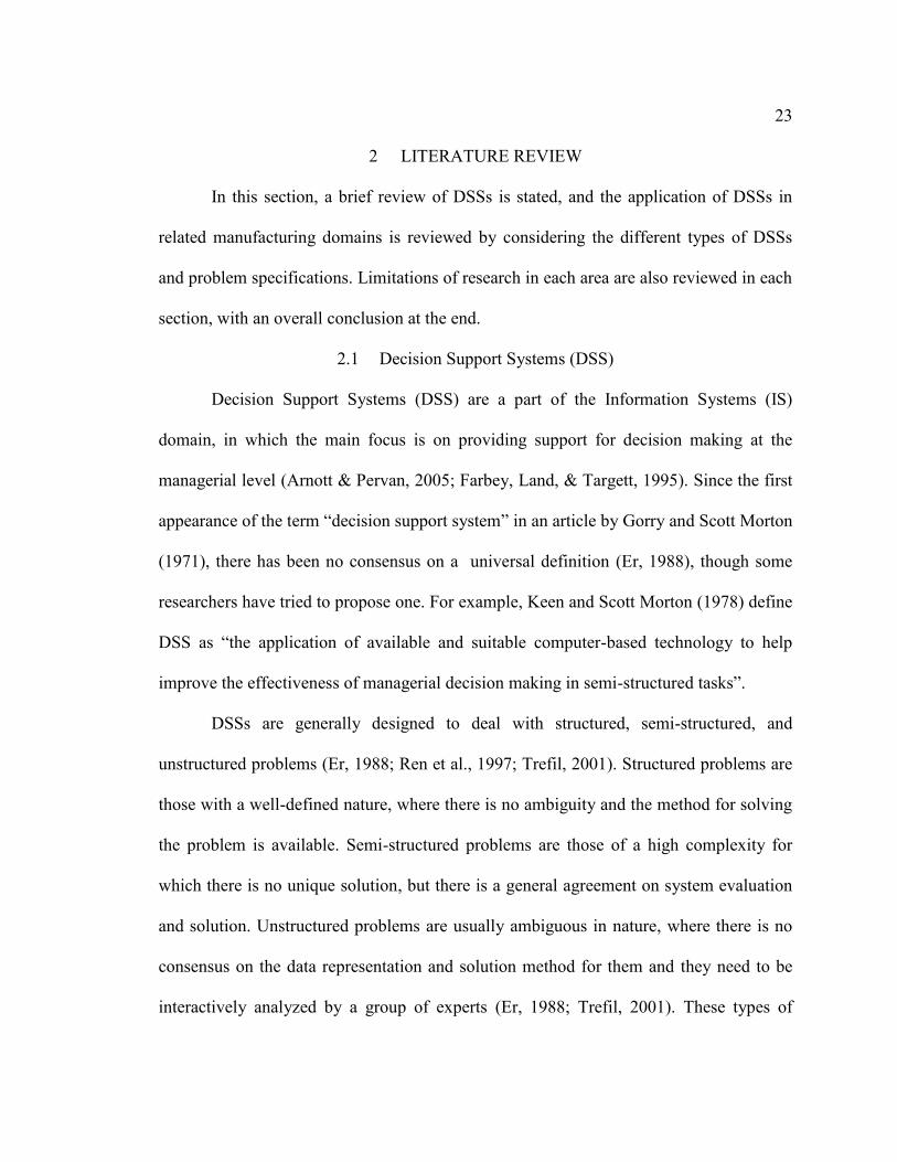
(Arnott & Pervan, 2005). Figure 1, adopted from Arnott and Pervan (2005), shows the

evolution of different DSSs in their time and origin.

26

Figure 1. Evolution and progress of DSSs in time

DSSs can be categorized according to two criteria of interaction and use (Alves,

da Silva, & Varela, 2013). The first taxonomy, shown in Table 1 and adopted from Bihl

et al. (2013), is proposed by Haettenschwiler (2001) and based on human interaction. It

divides DSSs into active, cooperative, and passive types. The second taxonomy,

summarized in Table 2 and adopted from Bihl et al. (2013), is based on use, and divides

DSSs into those which are communication driven, data driven, document driven,

knowledge driven, or model driven (D. Power, 2002).

27 Table 1. DSS interaction taxonomy (Haettenschwiler, 2001)

Type Description

Active Provide suggestions or state solutions to complex problems

Cooperative

Most complicated

Require the most interaction between the DSS and the human decision-

makers

Iterative approach:

1. Provide example solution

2. User modifies system parameters

3. DSS refines until arrival at a compromised solution

Passive Not designed to determine a solution explicitly for decision-makers

Table 2. DSS use taxonomy (D. Power, 2002) Type Description

Communication Driven Provide information to groups working on shared tasks

Data Driven Emphasize retrieval of real-time (or historic) internal or

(extra data)

Document Driven Integrates collected stored and processing technologies to

assist a decision maker with information retrieval

Knowledge Driven Derive specific recommendations for decision makers from

computer-driven and expert information

Model Driven Provide insight from mathematical models on perceived

phenomena

28

DSSs have been widely employed in corporate functional and non-corporate

applications (H. B. Eom & Lee, 1990; S. Eom & Kim, 2005; S. B. Eom, Lee, Kim, &

Somarajan, 1998). Corporate functional applications DDSs have been used in include

finance (Serrano-Cinca & Gutiérrez-Nieto, 2013), human resources (Broderick &

Boudreau, 1992), marketing (P. S. Balakrishnan, Jacob, & Xia, 2010), inventory

(Achabal, McIntyre, Smith, & Kalyanam, 2000), scheduling (L. Lin, Cochran, & Sarkis,

1992), forecasting (Guo, Wong, & Li, 2013), transportation (Y. Liu et al., 2010),

production (Tabucanon, Batanov, & Verma, 1994), and strategic management (Cebeci,

2009).

DSSs also have a variety of applications in non-corporate cases such as

agriculture (J. Liu, Wu, Tao, & Chu, 2013), education (Litvin et al., 2012), government

(Shan, Wang, Li, & Chen, 2012), healthcare (Beliën, Demeulemeester, & Cardoen,

2009), military (Song, Ryu, & Kim, 2010), natural resources (Newton, 2012), and

urban/community planning (Poole, Courtney, Lomax, & Vedlitz, 2009). In the rest of this

section, the application of DSSs in revenue management, forecasting, cost estimation,

planning and scheduling, and inventory will be investigated in more detail and the

limitations of existing literature will be examined.

2.2 Pricing and Revenue Management Systems

Revenue management is a field in which the focus is on maximizing revenue by

managing factors such as price and the distribution channels of goods and services

(Chiang, Chen, & Xu, 2007). The first applications of revenue management date back to

around 45 years ago in the airline industry (Chiang et al., 2007), and gradually have

29 found their way to many other areas such as hospitality industries (Kimes, 2005), health

care (Lieberman, 2004), retailing (Tsai & Hung, 2009), and manufacturing (Barut &

Sridharan, 2005).

Revenue management problems in manufacturing can be classified into three

major areas; market analysis, capacity planning, and pricing (Cheraghi, Dadashzadeh, &

Venkitachalam, 2010). In market analysis, the focus is on market segmentation and

forecasting. In capacity planning, inventory management and planning/scheduling are

mostly discussed. In pricing, based on the configuration of the system – i.e. make-to-

stock or make-to-order – the pricing techniques are the main concern. Figure 2 shows the

related areas of revenue management in manufacturing.

Figure 2. Areas of revenue management in manufacturing

30

Literature related to market analysis and capacity planning – i.e. forecasting,

planning/scheduling and inventory management – will be discussed in future sections. In

this section, the focus will be on pricing decision support systems.

Following the categorization of DSSs by Power (2002) that were introduced in

the previous section, Table 3 summarizes the literature of pricing and revenue

management systems in manufacturing.

Table 3. Categorization of pricing and revenue management systems in manufacturing literature based on different types of DSSs Communication

Driven Data Driven

Document

Driven

Knowledge

Driven Model Driven

(Hilton,

Swieringa, &

Turner, 1988)

(Bennavail,

Harding, &

Spears, 1990)

(Woo, Levy, &

Bible, 2005)

(Singh, 1991)

(Casey &

Murphy, 1994)

(Green &

Krieger, 1992)

(Krasteva,

Singh, Sotirov,

Bennavail, &

Mincoff, 1994)

(Albers, 1996)

(Cassaigne &

Singh, 2001)

(Yan, 2011)

As it can be observed from Table 3 , most of the literature involved in the

application of DSSs for pricing in manufacturing is in data- and model-driven DSSs. In

31 data-driven DSSs, the focus is on the historical data available from the past. In model-

driven DSSs, developing mathematical models that justify the relationship between

pricing and the inventory or sales amount are the main concern. In knowledge-driven

DSSs, expert systems have been used to choose the right price for products.

Reviewing Table 3 reveals some of the gaps and limitations of the literature. For

example, despite the potential usage advantages of communication-driven DSSs in

regards to pricing, these systems have not been investigated in this area. Also, the

integration of pricing and capacity planning is not completely investigated in literature.

Integration of pricing, the different aspects of capacity planning in a manufacturing firm,

and other related processes such as cost estimation continue to remain the main

limitations and gaps in literature in terms of the application of DSSs in pricing for

manufacturing.

2.3 Forecasting Support Systems

Although the forecasting problem is not tackled in this research directly, since a

part of the proposed decision support system receives the forecasted demand from the

expert, a brief literature review regarding forecasting support systems is included.

Within a manufacturing company, forecasting issues can be categorized into three

domains of design; selection, specification and evaluation issues (Winklhofer,

Diamantopoulos, & Witt, 1996). In each category there are some key elements for a

decision maker to decide about. In design, common questions include:

What is the purpose of forecasting?

32

How frequently should the forecasting be conducted, and what is

the time horizon of forecasting?

What kind of resources do we need?

Who should do the forecasting?

Who is going to use the results?

What are the data resources?

In selection and specification, one has to deal with questions such as:

What forecasting method can be applied?

Is it necessary to use multiple techniques?

At the evaluation level, a decision maker may face questions such as:

How can a forecast result be displayed and presented for

management?

Is it necessary to take into account the subjective judgment of

experts about forecasting? If yes, how?

What metrics are needed for forecasting evaluations?

How is it possible to address the forecasting problem more

efficiently and improve it?

An answer to each one of these questions can have a great impact on the profit of

a manufacturing plant in terms of internal factors such as capacity usage, inventory costs,

workforce assignment, etc., and external factors such as market share and stock price

(Hirst, Koonce, & Venkataraman, 2008; Mahmoud, Rice, & Malhotra, 1988; Raturi,

Meredith, McCutcheon, & Camm, 1990; Wright, 1988). For finding a suitable answer to

33 these issues, it is necessary to take advantage of existing models, such as time series,

artificial neural networks, and expert judgment (Fildes, Nikolopoulos, Crone, & Syntetos,

2008; Goodwin, Fildes, Lawrence, & Nikolopoulos, 2007; Lawrence, O'Connor, &

Edmundson, 2000; Webby, O'Connor, & Edmundson, 2005; Winklhofer &

Diamantopoulos, 2003). Figure 3, adopted from (Winklhofer et al., 1996), depicts these

issues and their corresponding domains and topics of decision making.

A forecasting support system (FSS) is a software framework which takes

advantage of expert judgment, mathematical techniques, and past data integration in

order to assist decision makers in forecasting and analyzing the results (Adya & Lusk,

2012; Armstrong, 2001; Fildes, Goodwin, & Lawrence, 2006). In other words, FSS is

where DSS meets forecasting techniques. In this sense, FSSs can also be classified based

on DSSs and forecasting issues. Table 4 summarizes various research conducted in FSSs

in manufacturing.

34

Figure 3. Design, selection/specification and evaluation issues in forecasting (adopted from (Winklhofer et al., 1996))

Table 4. Different types of forecasting support systems designed for different forecasting issues

DSS Type Design Selection/Specification Evaluation

Communication

Driven

(Cheikhrouhou,

Marmier, Ayadi, &

Wieser, 2011)

Data Driven

Document Driven

35 Table 4: continued

Knowledge Driven (Wen, 2007)

(R. Kuo & Xue, 1998)

(R. Kuo, 2001)

(R. J. Kuo, Wu, &

Wang, 2002)

(Petrovic, Xie,

& Burnham,

2006)

Model Driven

(Winklhofer &

Diamantopoulos, 2003)

(Sun, Choi, Au, & Yu,

2008)

(Ching-Chin, Ka Ieng,

Ling-Ling, & Ling-

Chieh, 2010)

(Xia, Zhang, Weng, &

Ye, 2012)

(Guo et al., 2013)

(Korpela & Tuominen,

1996)

(Venkatachalam & Sohl,

1999)

(Thomassey, Happiette,

& Castelain, 2005)

(J. D. Bermúdez,

Segura, & Vercher,

2006)

(J. D. Bermúdez,

Segura, & Vercher,

2007)

(J. Bermúdez, Segura, &

Vercher, 2008)

(C.-T. Lin & Lee, 2009)

(Sayed, Gabbar, &

Miyazaki, 2009)

(Caliusco,

Villarreal,

Toffolo,

Taverna, &

Chiotti, 1998)

(Zhong, Pick,

Klein, & Jiang,

2005)

(Dellarocas,

Zhang, &

Awad, 2007)

(Ali, Sayın,

Van Woensel,

& Fransoo,

2009)

(Efendigil,

Önüt, &

Kahraman,

2009)


(Corberán-Vallet,

Bermúdez, Segura, &

Vercher, 2010)

(Poler & Mula, 2011)

(Wagner, Michalewicz,

Schellenberg, Chiriac, &

Mohais, 2011)

(Y. Yu, Choi, & Hui,

2011)

(Aksoy, Ozturk, &

Sucky, 2012)

(J. D. Bermúdez,

Segura, & Vercher,

2012)

According to the publications reviewed in Table 4 , the most investigated area is

in the application of model-driven DSSs in selection and specification issues in

forecasting. Among the different types of DSSs applied, no application regarding the

data-driven and document-driven DSSs has been found, and only one publication

addresses the communication-driven DSSs. The second area of focus has been on

knowledge-driven DSSs. Although various research has been dedicated to FSSs, there are

some limitations and gaps which will be stated briefly.

37

Design issues in forecasting mostly address fundamental questions such as the

purpose of forecasting, time horizon definition, and data sources selection. Most of the

problems faced in this domain are semi-structured or unstructured. For example, it is hard

to structurally answer the question, “What data sources can be used for prediction?”

Hence, the models developed in literature for this purpose are limited and mostly focused

on time horizon definition. On the other hand, the opinion of an expert seems to be of

high value in this domain, and so the importance of communication-driven DSSs become

more obvious. However, a limited number of publications have considered this issue.

Considering the nature of design issue in forecasting, integration also seems to be

a significant need. There are a few research papers dedicated to this subject, and in all of

them, only the integration with marketing is considered (Cheikhrouhou et al., 2011;

Winklhofer & Diamantopoulos, 2003).

The same limitations and gaps already mentioned for design are observed with

selection and specification – i.e. a lack of communication-driven DSSs involving

application and integration. Additionally, the scope of the concept of selection and

specification in most of the research is considered in only a limited format. For example,

model selection in most of the papers is bound to a selection of parameters of a specific

method—such as exponential smoothing—but no research is dedicated to any

comparison between different methods, such as artificial neural networks and time series.

Lack of proper integration and usage of communication-driven DSSs is also a part

of the limitations and gaps in evaluating forecasting issues. The amount of research

38 focused on integration is limited, and the integration doesn’t consider design issues

(Caliusco et al., 1998).

In general, three major limitations and gaps can be found regarding FSS research

in literature. The first limitation corresponds to the application of communication-driven

FSSs, which can have a high potential in improving the FSSs due to the incorporation of

expert opinion. Second, enough integration has not been addressed in literature, and there

a lot of missing chains between FSSs and other organizational processes which can be

explored and established. Third, due to the complexity of decisions made by FSSs, any

comparison between different methods is not considered in each domain.

2.4 Cost Estimation Decision Support Systems

Cost estimation covers a wide spectrum of manufacturing systems, from the

feasibility and evaluation of new products to the after-sale services (Layer, Brinke,

Houten, Kals, & Haasis, 2002). There are four basic methods for cost estimation--

namely, intuitive, analogical, parametric, and analytical methods (Duverlie & Castelain,

1999). In an intuitive method, the cost of a product is estimated based on the expert’s

knowledge. In an analogical method, the cost of a product is estimated based upon the

cost of similar products. The parametric method takes advantage of a product’s

parameters and uses them to evaluate the cost. In an analytical method, the emphasis is

on the works required to build a product.

Each of these cost estimation methods can be applied in different phases of

product development. Figure 4, adopted from Duverlie and Castelain (1999), depicts the

application of each cost estimation method to a different phase of product development.

39 As one can observe, parametric methods are more often used in early stages of product

development, while analytic methods are mostly used in later phases. Analogical methods

are used in both early and later phases. Intuitive methods can be applied in all stages.

Figure 4. Different methods of cost estimation and their application in different stages of product development (adopted from Duverlie and Castelain (1999))

In order to review the literature of cost estimation decision support systems,

different methods of cost estimation and different types of DSSs will be considered.

Table 5 lists the existing literature regarding DSSs, based on various cost estimation

methods.

40 Table 5. Different types of DSSs designed based on various cost estimation methods

DSS Type intuitive Analogical Parametric Analytical

Communication

Driven

Data Driven

(Koonce, Judd,

Sormaz, &

Masel, 2003)

(Mauchand,

Siadat, Bernard,

& Perry, 2008)

(Quintana &

Ciurana, 2011)

(Darla &

Narayanan,

2013)

(Eaglesham,

1998)

(Ben-Arieh,

2000)

(Park &

Simpson*,

2005)

(Dai,

Balabani, &

Seneviratne,

2006)

Document

Driven

Knowledge

Driven

(Rush & Roy,

2001)

(De Souza, 1995)

(Chin & Wong,

1996)

(Kingsman & de

Souza, 1997)

(Bode, 1998)

(Shehab &

Abdalla, 2001)

(SOUZA &

KINGSMAN,

1999)


(Brinke, 2002)

(H. Wang,

Ruan, & Zhou,

2003)

(Wasim et al.,

2013)

Model Driven

As one can observe from Table 5, most of the research existing in literature

belongs to parametric- and analytic-based methods of cost estimation. Only a few

publications are devoted to intuitive and analogical methods. Additionally, the most

common types of DSSs used in cost estimation are data-driven and knowledge-driven

DSSs.

Most of the publications in cost estimation are solely devoted to cost estimation,

and only a few of them consider the integration of cost estimation with other related areas

such as pricing and scheduling. Usage of model-driven DSSs also remains largely

ignored in literature.

2.5 Planning and Scheduling Support Systems

Scheduling and sequencing play a significant role in manufacturing, and are

considered to be an important aspect of decision making on the shop floor (Pinedo,

2012). Generally speaking, the goal of scheduling is to arrange and sequence the jobs on

different machines in order to optimize resource consumption (Pinedo, 2012). A

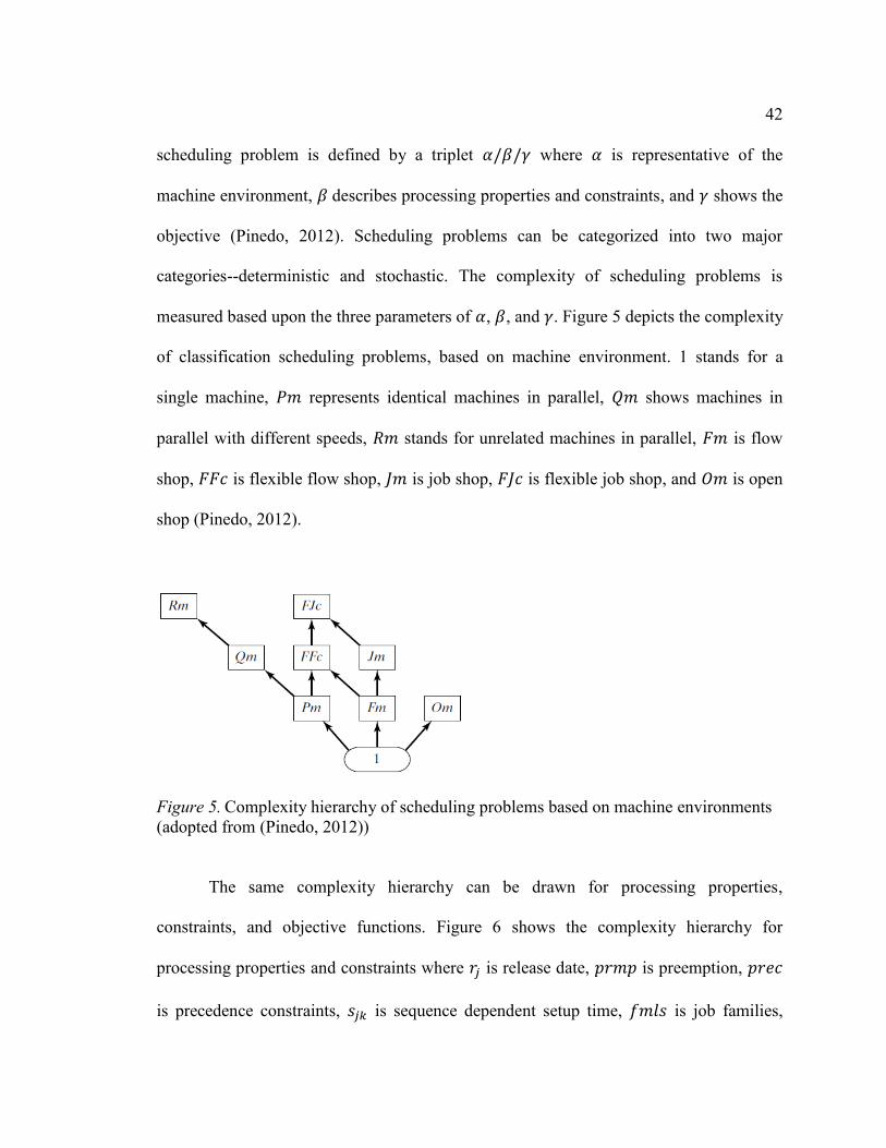
42 scheduling problem is defined by a triplet where is representative of the

machine environment, describes processing properties and constraints, and shows the

objective (Pinedo, 2012). Scheduling problems can be categorized into two major

categories--deterministic and stochastic. The complexity of scheduling problems is

measured based upon the three parameters of , , and . Figure 5 depicts the complexity

of classification scheduling problems, based on machine environment. 1 stands for a

single machine, represents identical machines in parallel, shows machines in

parallel with different speeds, stands for unrelated machines in parallel, is flow

shop, is flexible flow shop, is job shop, is flexible job shop, and is open

shop (Pinedo, 2012).

Figure 5. Complexity hierarchy of scheduling problems based on machine environments (adopted from (Pinedo, 2012))

The same complexity hierarchy can be drawn for processing properties,

constraints, and objective functions. Figure 6 shows the complexity hierarchy for

processing properties and constraints where is release date, is preemption,

is precedence constraints, is sequence dependent setup time, is job families,

43 is batch processing, is breakdown, is machine eligibility

restrictions, is permutation, is blocking, is no wait, and is

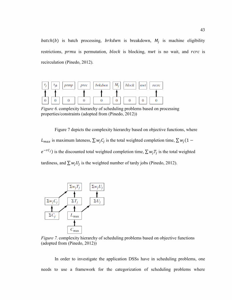
recirculation (Pinedo, 2012).

Figure 6. complexity hierarchy of scheduling problems based on processing properties/constraints (adopted from (Pinedo, 2012))

Figure 7 depicts the complexity hierarchy based on objective functions, where

is maximum lateness, ∑ is the total weighted completion time, ∑

is the discounted total weighted completion time, ∑ is the total weighted

tardiness, and ∑ is the weighted number of tardy jobs (Pinedo, 2012).

Figure 7. complexity hierarchy of scheduling problems based on objective functions (adopted from (Pinedo, 2012))

In order to investigate the application DSSs have in scheduling problems, one

needs to use a framework for the categorization of scheduling problems where

44 importance of data is also taken into account. Unfortunately, since the focus of the

traditional scheduling classification is more on theoretical aspects rather than

applicability and information (Framinan & Ruiz, 2010), it cannot be used for exploring

DSSs’ application in scheduling completely, and only a few papers have proposed DSSs

based upon traditional classification (Adler et al., 1993; Belz & Mertens, 1996; Josef

Geiger, 2011; Kungwalsong & Kachitvichyanukul, 2006; Viviers, 1983). On the other

hand, due to the high complexity of real world scheduling systems, it is often hard to

induct them into one of the traditional categories. For these reasons, the focus of this

research will be on the information flow diagram proposed by Pinedo (2012), in which

scheduling is considered to be a part of more comprehensive schema of planning and

scheduling. Figure 8 shows an information flow diagram in a manufacturing system. The

chart is composed of three main parts--namely planning, scheduling and dispatching, and

shop floor management and control. Application of DSSs in scheduling and planning can

be also be categorized by following this diagram.

45

Figure 8. Information flow chart in manufacturing (adopted from (Pinedo, 2012))

Table 6 summarizes various research conducted on PSSs, keeping in mind the

industry type and categorization of DSSs proposed by Power (2002).

Table 6. Different types of planning support systems designed for different scheduling and planning problems

DSS Type Planning Scheduling Shop floor

management/control

Communication Driven

General:

(F. T. Chan, Jiang, & Tang, 2000)

General:

(Makarouni, Psarras, & Siskos, 2013)



Agricultural Engine:

(Özdamar, Bozyel, & Birbil, 1998)

General:

(De Vin, Ng, Oscarsson, & Andler, 2006)

General:

(Grabot, Blanc, & Binda, 1996)

Data Driven

Wood:

(Buehlmann, Ragsdale, & Gfeller, 2000)

Comp. Man.

Systems:

(P. Chen & Talavage, 1982)

(Dilts, Boyd, & Whorms, 1991)

Semi-conductor:

(Fordyce, Dunki‐Jacobs, Gerard, Sell, & Sullivan, 1992)

Document Driven

General:

(Bistline Sr, Banerjee, & Banerjee, 1998)

General:

(Kan & Chen, 2013)

(Jindal et al., 2013) (K.-S. Wang, Hsia, & Zhuang, 1995)

(W.-H. Kuo & Hwang, 1998)

(Novas & Henning, 2009)

Knowledge Driven (Shaw, 1988)

(Tsadiras, Papadopoulos, & O’Kelly, 2013)

(Yamaha, Matsumoto, & Tomita, 2008)

Power Plants:

(Aoyagi, Tanemura, Matsumoto, Eki, & Nigawara, 1988)


Knowledge Driven Food:

(Henning & Cerdá, 2000)

General:

(Borenstein, 1998)

General:

(Belz & Mertens, 1996)

General:

(McConnell & Medeiros, 1992)

(Escudero, Kamesam, King, & Wets, 1993) (Josef Geiger, 2011)

Electronics:

(L. Lin et al., 1992)

(Kungwalsong & Kachitvichyanukul, 2006)

(Kapanoglu & Miller, 2004)

(Mallya, Banerjee, & Bistline, 2001)

(Kazerooni, Chan, & Abhary, 1997)

(McKay & Wiers, 2003) (Kim & Kim, 1994)

(Tsubone, Matsuura, & Kimura, 1995)

(H. Li, Li, Li, & Hu, 2000)

Wood:

(Farrell & Maness, 2005)

(Madureira, 2005)

Model Driven Appliances:

(Gazmuri & Arrate, 1995)

(Mahdavi, Shirazi, & Solimanpur, 2010)

Ship building:

(Lee et al., 1995)

(Trentesaux, Dindeleux, & Tahon, 1998)

Textile:

(Mok, Cheung, Wong, Leung, & Fan, 2013)

(Tsukiyama & Mori, 1991)

(Viviers, 1983) (Wiendahl &

Garlichs, 1994)

(M.-F. Yang & Lin, 2009)

Packaging:

(Adler et al., 1993)

Ion Plating:

(F. T. Chan, Au, & Chan, 2006)


Refinery:

(Chryssolouris, Papakostas, & Mourtzis, 2005)

Steel:

(Cowling, 2003)

(Karumanasseri & Abourizk, 2002)

(Tamura, Nagai, Nakagawa, Tanizaki, & Nakajima, 1998)

Model Driven Chemical:

(Escudero et al., 1993)

Electronics:

(Jeong, Leon, & Villalobos, 2007)

Turbine

Manufacturing:

(Krishna, Mahesh, Dulluri, & Rao, 2010)

Pottery:

(Petrovic & Duenas, 2006)

Tobacco:

(Van Dam, Gaalman, & Sierksma, 1998)

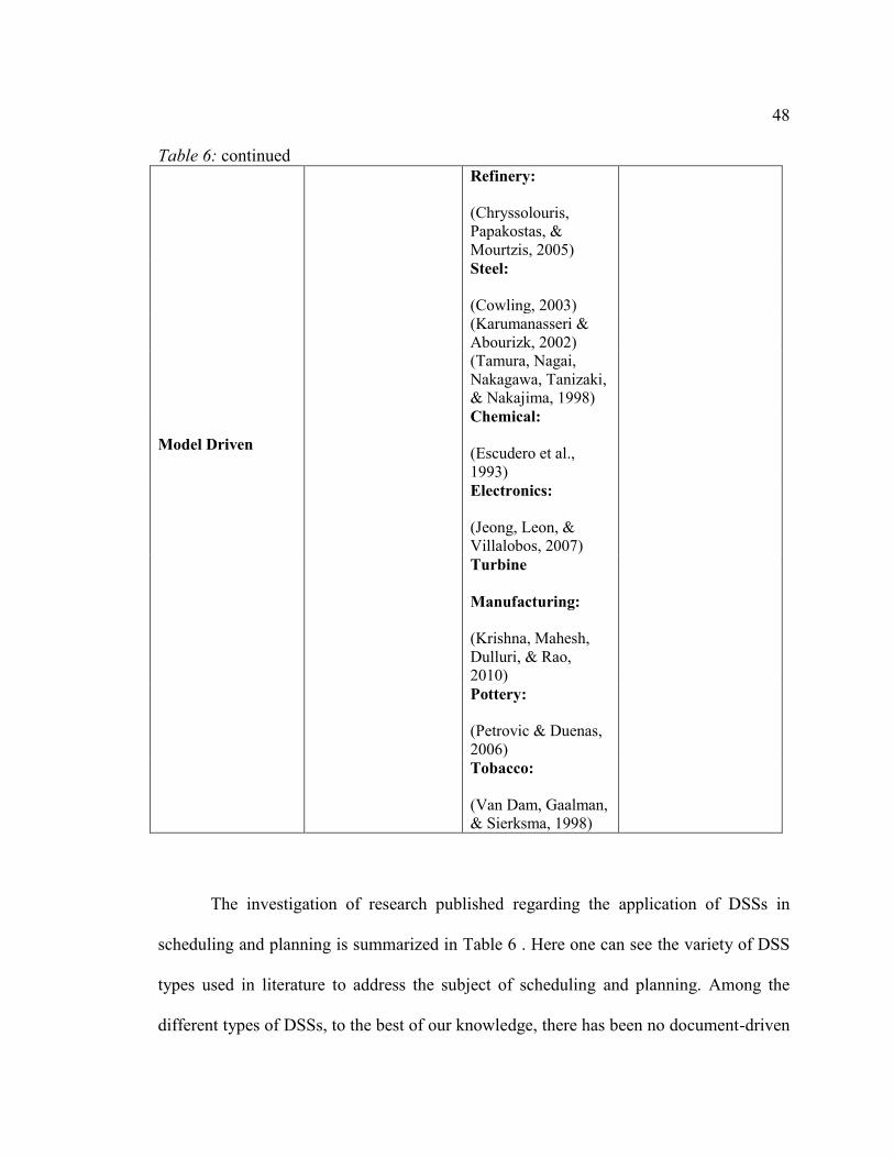
The investigation of research published regarding the application of DSSs in

scheduling and planning is summarized in Table 6 . Here one can see the variety of DSS

types used in literature to address the subject of scheduling and planning. Among the

different types of DSSs, to the best of our knowledge, there has been no document-driven

49 DSS applied to scheduling and planning, which seems justified, if one considers the

description of this type of DSS listed in Table 2 and the nature of scheduling and

planning. Among the other DSSs, most practices belong to model-driven and knowledge-

driven DSSs which seems reasonable if one takes into account the well-defined nature of

scheduling/planning.

Among various levels of the problematic domain – i.e. planning, scheduling, and

shop floor management/control – the least investigated and the most investigated levels

are control and scheduling, respectively. Since the application of control systems is

limited due to the availability of the data for real-time decision making, most of the

research in this area is related to data-driven DSSs. Most of the application-based

research is reported in the scheduling and planning level. Although much research has

been conducted regarding the application of DSSs in planning and scheduling, there are

still some gaps and limitations one finds in the literature, which will be discussed briefly.

In planning, most of the research is focused on model-driven DSSs, which, when

one considers the long-term and semi-structured nature of planning and the axiomatic

management role in DSSs, it seems that there has been not enough research in

communication-driven DSS application. This drawback will become clearer when one

considers the planning issue as a problem where many different experts need to get

involved in order to create the best outcome.

Additionally, a good plan should be feasible and consistent with other decisions

such as scheduling, forecasting, inventory, and marketing in an organization. In this

regard, the integration of planning with other systems becomes favorable. However, in

50 literature not much research has focused on this issue (Kungwalsong &

Kachitvichyanukul, 2006; Lee et al., 1995; Özdamar et al., 1998), and the only

integration is between planning and scheduling.

Another drawback of literature in this regard is a lack of probabilistic

considerations in planning, which due to its medium- to long-term time horizon, seems

necessary to consider. In addition, no mechanism was introduced for a correction of the

plan when there has been a deviation from the goal.

Like planning, the scheduling literature also suffers from a lack of integration and

correction procedures. Furthermore, since the scheduling problem has a short-term

horizon and hence, real time data may be important, it seems that data-driven DSSs can

be investigated further in this domain.

In spite of planning and scheduling, most of the research on shop floor

management/control is integrated with scheduling (P. Chen & Talavage, 1982; Dilts et

al., 1991; Fordyce et al., 1992; Grabot et al., 1996; Kan & Chen, 2013; K.-S. Wang et al.,

1995), but there is still not a complete integration between control, scheduling, and

planning.

In general, the integration of planning and scheduling support systems with other

processes in an organization, probabilistic considerations, and correction procedures

remain the main drawback and literature gap in this domain.

2.6 Inventory Management Systems

Inventory problems can be categorized into three different levels; namely,

strategic, tactical, and operational (Peidro, Mula, Poler, & Lario, 2009; Rouwenhorst et

51 al., 2000), which cover long-term, medium-term, and short-term decision making for

planning, respectively (Gupta & Maranas, 2003).

At the strategic level, the questions that should be addressed include:

How should one design process flow?

What type of technical systems should be selected and how?

At the tactical level, a decision maker may face the questions including:

How does one do dimensioning of the storage system?

How does one define the layout?

What kind of equipment should be selected?

How should one design the organization of inventory?

At the operational level, the problems are of a short-term nature, such as:

How does one fine tune the organization’s policies?

How does one assign a work force to different tasks?

How does one sequence pickings? How does one assign docks for

shipping?

In order to investigate the role of decision support systems in inventory, the same

categorization – i.e. strategic, tactical, and operational – will be used. Table 7 summarizes

various research conducted in inventory and DSSs. The same classification of DSSs used

for planning and scheduling is copied here (D. Power, 2002).

52 Table 7: Different types of planning support systems designed for different inventory problems’ level

DSS Type Strategic Tactical Operational


(Achabal et al., 2000) (P.-C. Yang & Wee, 2006)

(Chande, Dhekane, Hemachandra, & Rangaraj, 2005)

(Natarajan, 1989)

(Banerjee & Banerjee, 1992)

(Kagami, Homma, Akashi, Aizawa, & Mori, 1992)

Data Driven (Manthou & Vlachopoulou, 2001)

(Moole & Korrapati, 2004)

(Van Donselaar, van Woensel, Broekmeulen, & Fransoo, 2006)

Document Driven

Knowledge Driven (Prasad, Shah, & Hasan, 1996) (Ehrenberg, 1990)

(Tu et al., 2007)

(Moynihan, Raj, Sterling, & Nichols, 1995)

(Retzlaff-Roberts & Amini, 1998) (Williams, 1984)

(Min, 2009) (Sobotka, 1998) (Cohen, Kamesam, Kleindorfer, Lee, & Tekerian, 1990)

(Badri, 1999) (Agrell, 1995)

(Disney, Naim, & Towill, 2000)

(Chaudhry, Salchenberger, & Beheshtian, 1996)

Model Driven (J. Walker, 2000) (H.-G. Chen & Sinha, 1996)

(H.-h. YU & SUN, 2002)

(Towill, Evans, & Cheema, 1997)

(Razi & Tarn, 2003) (Samanta & Al-Araimi, 2001)

(Signorile, 2005) (Disney & Towill, 2005)

(Woo et al., 2005) (Cheng & Chou, 2008)


(Goel & Gutierrez, 2006)

(Qingsong & Lizhi, 2010)

(Lo, 2007) (Zeng, Wang, &

Zhang, 2007)

(Cakir & Canbolat, 2008)

(S. Li & Kuo, 2008)

Model Driven (Shang, Tadikamalla, Kirsch, & Brown, 2008)

(Southard & Swenseth, 2008)

(Yazgı Tütüncü, Aköz, Apaydın, & Petrovic, 2008)

(Zhang, Hua, & Xu, 2009)

(Borade & Bansod, 2011)

(Cadavid & Zuluaga, 2011)

Review of research tabulated in Table 7 shows that most of the research on the

application of DSSs for inventory belong to model-driven DSSs and on the tactical level

of decision making. Among the DSSs, there has been no example found of document-

driven DSSs in literature. Most of the research is dedicated to model-driven and data-

driven DSSs. At the strategic level, only one research paper has been found. At the

tactical level, where the problems are well-defined and structured, the focus has been on

model -riven DSSs, while at the operational level (where the problems are usually of a

short-term nature), most of the research was concentrated on data-driven DSSs. Notice

that since in short-term decision making the accessibility of the data is important, data-

driven DSSs play a more important role.

54

Although much research has been dedicated to the application of DSSs in

inventory, there are some limitations and gaps, which will be discussed briefly.

Inventory problems tend to be semi-structured or unstructured at the strategic

level, and hence naturally need expert opinion. In this sense, knowledge-driven and

communication-driven DSSs may be of great help. However, this issue has not been

covered in literature. Additionally, reviewing the problem at a strategic level demands a

strong integration with other units of the organization, such as the production, marketing,

tactical, and operational levels. No research considering this issue has been found in this

literature review. The applicability of literature on DSSs at the strategic level of inventory

decision making also remains an open investigation.

Similar to the strategic level, at the tactical level the literature also suffers from

the lack of comprehensive integration. However, unlike at the strategic level, more

research has been conducted regarding communication-driven DSSs. Since the decisions

in this level are medium-term and still of a semi-structured nature in some areas, the

application of expert knowledge seems to be of great help, though this has not been

explored comprehensively in literature.

A lack of comprehensive integration also remains a limitation regarding the

application of DSSs at the operational level of inventory. Perhaps the only level in which

the usage of document-driven DSSs seems to be justified in an inventory is at the

operational level. The reason can be the need for documents, which have to be issued for

each transaction in inventory. This issue has not been addressed in literature.

55

2.7 Limitations

A review of decision support systems’ (DSS) history, evolution, taxonomy, and

application in planning/scheduling, forecasting, and inventory for manufacturing was

proposed. Different levels of problems for planning/scheduling, forecasting, and

inventory was investigated according to the taxonomy offered by literature. The

limitations and gaps of research in this area literature were also briefly explored.

In pricing and revenue management, integration with other related areas of

manufacturing such as cost estimation, scheduling, and inventory, as well as the lack of

exploration in communication-driven DSSs, remain the main gaps and limitations in

literature.

In planning and scheduling, there was a lack of enough research regarding the

applications of communication-driven and knowledge driven-DSSs, proper and

comprehensive integration, testing, probabilistic considerations, and correcting

procedures.

In forecasting, the main limitations and gaps were lack of enough research in the

applications of communication-driven and knowledge-driven DSSs, proper and

comprehensive integration, applicability and real world testing in many cases, and of

considering various models for decision making.

In cost estimation (a particularly important activity in manufacturing), integration

with other relevant areas such as pricing, planning, scheduling, inventory, and marketing

has not been explored enough in literature.

56

Regarding inventory, lack of enough research in the application of

communication-driven, knowledge-driven and document-driven DSSs; lack of a proper

and comprehensive integration; lack of applicability and enough testing in much of the

research; lack of probabilistic considerations; and lack of correcting procedures remain

the main limitations and gaps in literature.

57

3 GENERAL FRAMEWORK OF THE SYSTEM

In this section the general framework of the system is described. The proposed

decision support system has four modules. The output of each module can be the input to

another module. Figure 9 depicts the General framework and modules of the proposed

decision support system.

Pricing and Planning

Robust Optimization

Cost Estimation

Analytical Cost Estimation

Cost of Products

Demand Prediction Expert

Data Base

Flow Process Chart

Shop Floor

Warehouse

Scheduling

Simulation Optimization

Plan

Activities

Inventory Level and Costs

Flow Process Chart

Skill LevelFlow Process Chart

Inventory

Mathematical Modeling

Plan

Schedule

Capacity and Lead Times

Figure 9. General framework and modules of the proposed decision support system

The proposed system is interactive in the sense that it is able to suggest new

solutions based on the data it obtains from the shop floor and the demand information

that it receives from the expert interactively. The data acquired from the shop floor and

58 the warehouse is stored in a database. The structure of this database will be covered

partially in next chapters wherever necessary.

3.1 Cost Estimation

The first module of the system is cost estimation. This module estimates the

finished costs, inventory cost and the lost sale cost for each product. The inputs of this

module are the cost occurred and the cost centers defined by the user. Cost centers are the

entities that store the expenses. For instance, a machine in production line can be a cost

center. All the expenses related to purchase, maintenance and operation of each machine

are stored in the cost center associated with that machine and will be used to calculate the

finished cost of the products that use that machine. This module is explained in detail in

section ‎4.

3.2 Pricing and Planning

The outputs of cost estimation module are used in pricing and planning module

for obtaining the optimum set of prices and production plan for each product in each

period. In pricing and planning module the demand is considered to be uncertain and

price dependent. For this purpose, for each price point a minimum and maximum demand

is defined by the expert. To incorporate the uncertainty of the demand in the decision

making process, a robust optimization model will be formulated for the problem. This

model will be solved using an exact method and a metaheuristic named unconscious

search (US). This module is explained in detail in section ‎5.

59

3.3 Scheduling

The output of pricing and planning module will be used in scheduling module.

This part of the system schedules the jobs created by pricing and planning. For this

purpose, a simulation optimization method is used in which the processing time of the

jobs in each working station is considered probabilistic. Scheduling module tries to

obtain the best sequence of jobs on the production line using a variable neighborhood

search (VNS). To schedule a single job, it is simulated on the production line several

times and the tasks that appear on the critical path are given higher priority for

scheduling. This module is explained in detail in section ‎6.

3.4 Inventory

The last module of the system is inventory. This module tries to minimize the

inventory costs using a mathematical model and the inputs from scheduling and pricing

and planning modules. To solve the mathematical model of the inventory, an exact

method and a tabu search are applied. This module is explained in detail in section ‎7.

60

4 FINANCIAL AND COST ESTIMATION MODULE

The decision support system introduced in this research has several modules. In

this chapter, the financial and cost estimation module is introduced, and its inputs,

processes, methods, and outputs are described.

4.1 Inputs

The financial and cost estimation module has several inputs. Each input comes

from an interaction of a user with a system or another module. The inputs of the system

are described in the following sub-sections.

4.1.1 Cost Centers

The first inputs of financial and cost estimation modules are cost centers. Any

department or unit that a cost may charge into is considered a cost center. Here, two types

of cost centers are differentiated. The first type of cost center is an overhead. An

overhead cost center is any type of cost center that has the expenses unrelated to direct

labor and material included. Such cost centers include human resources and insurance.

Note that the overhead definition can be different based on the business type and

products. Since production-based businesses are dealt with in this research, the overhead

definition is also adjusted according to the needs of the type of business.

Beside overhead cost centers, there are operational cost centers in which the

expenses related to direct labor and direct material are recorded. These types of cost

centers include working stations, operators, production machines, work-in-process, and

materials purchased.

61

4.1.2 Costs

Other inputs of financial and cost estimation modules are the costs. A cost has

many components, including the amount, date, and type. The amount and date of the cost

help to determine the finished costs of products in a period. The type of cost helps to

distinguish between operational costs and preparing the balance sheets. To record a cost,

one needs to categorize it according to a predefined hierarchy. In practice, this hierarchy

has at least three levels/ledgers. The first level shows to which major category an expense

belongs, while the other two levels make the categorization more detailed. Figure 10

shows the relation of costs, cost types, and cost centers. To record a cost, one needs to

know to which cost center and cost type it belongs. Storing a cost in this format helps to

estimate various cost coefficients such as inventory, production, and lost sales cost. In

addition, this architecture enables a user to generate different reports based upon his/her

needs.

Figure 10. Relation of costs, cost types and cost centers

62

4.2 Processes

Having costs and cost centers as inputs, the financial and cost estimation module

includes three main processes. These processes are estimating finished costs, inventory

costs, and lot sale costs, based on an analytical cost estimation method. These three

expenses are used as outputs to a pricing and planning module of the decision support

system.

4.2.1 Estimating Finished Costs

To estimate the finished cost of a product, it is necessary to know which cost

centers are used to produce one unit of that product. It is possible that a cost center will

be used for several products. In this case, each product will get a share of the common

cost center, based upon the time it has spent in there. As an example, assume a situation

in which there are five products and five cost centers. Each cost center has some expenses

recorded in it, and each product has used a certain amount of time in each cost center.

Table 8 summarizes the time (hour) each product has spent in each cost center (CC) and

the total expenses recorded in each cost center. For calculating the finished cost, the

expenses in each cost center should be divided by the time-share of each product from

that cost center. Then, all the expenses of that product are added together. Thus, product

1, which has

time share of cost center 1, will absorb

of total expenses of CC1. Table 9 shows the share of each

product in each cost center and its associated finished cost. Note that these calculations

need to be done for each time period.

63 Table 8: The time (hour) each product spent on each cost center and the total expenses recorded in each cost center (CC)

CC 1 CC 2 CC 3 CC 4 CC 5

Prod. 1 22 21 18 12 16

Prod. 2 15 16 12 18 13

Prod. 3 21 15 24 23 14

Prod. 4 22 20 12 17 19

Prod. 5 12 22 16 18 11

Total expenses($) 1200 4500 1600 3200 2400

Table 9: Share of each product in each cost center and its finished cost CC 1 CC 2 CC 3 CC 4 CC 5 Finished Cost

Prod. 1 287.0 1005.3 351.2 436.4 526.0 2605.9

Prod. 2 195.7 766.0 234.1 654.5 427.4 2277.7

Prod. 3 273.9 718.1 468.3 836.4 460.3 2756.9

Prod. 4 287.0 957.4 234.1 618.2 624.7 2721.4

Prod. 5 156.5 1053.2 312.2 654.5 361.6 2538.1

4.2.2 Estimating Inventory Costs

For estimating the inventory cost, the hierarchical structure of the costs can be

used. For this purpose, each category in each level of the hierarchy can be marked with

the attribute of its inventory cost. This means that if a cost falls under a certain category,

its immediate level or its predecessor on the hierarchy is marked as inventory cost, and it

will be calculated towards inventory cost. For calculating the total inventory cost, all

64 these categories and the expenses recorded in them will be summed up. Obviously, the

inventory cost for a single unit is the total inventory cost divided by the total number of

units. Inventory cost can then be determined more precisely if the space occupied by each

product is also taken into account.

4.2.3 Estimating Lost Sale Cost

Estimating the lost sale cost is rather straightforward. In this research, the lost sale

cost is considered to be the profit that could be made by selling one unit of a product, but

was not made due to inventory level. For estimating this number, one needs to know the

finished cost and minimum expected profit of a product. In the case where the demand is

always greater than the production capacity, the lost sale cost tends to be 0. In the case

where lost sales can have dramatic effects on profitability, such as the cases in which

there are huge penalties for the late delivery of a product, the lost sale cost can be set to

infinity.

4.3 Design and Outputs of Finance and Cost Estimation Module

Financial and cost estimation modules have three main outputs; namely, finished

costs, inventory costs, and lost sale costs. These three parameters are very important in

building the models for the pricing and planning of products. Figure 11 shows the inputs,

processes, and outputs of finance and cost estimation modules.

65

Figure 11. Inputs, processes and outputs of finance and cost estimation modules

66

5 PRICING AND PLANNING MODULE

In this chapter, the pricing and planning module is explained in detail and the

inputs, processes, and outputs of the module are described. A robust optimization

methodology is applied for dealing with demand uncertainty. Since in real world

situations the dimension of the problem becomes very large and thus hard to tackle with

an exact method, a metaheuristic is introduced to solve large-scale pricing and planning

problems. The solutions of metaheuristics are verified by comparing to exact solutions

obtained using CPLEX Optimization Studio 12.3.

5.1 Inputs

The pricing and planning module has three sets of inputs. The first set is the

outputs of finance and cost estimation modules. The second set is the constraints of

resources, such as budget and space. The third set is the time periods and demands

obtained from experts. It is assumed that the expert uses a forecasting technique

according to his need, and hence the forecasting problem is not tackled in this research.

Rather, it is considered to be handled by the expert and interactively communicated to the

system. This assumption makes the system more flexible in the sense that the expert can

choose his/her specific method of forecasting, which is more compatible with the

business type and its market. In addition, with any change in the demand pattern, the

proposed decision support system can come up with a new strategy to improve the

profitability.

67

5.1.1 Inputs from Finance and Cost Estimation Module

The first set of inputs to a pricing and planning module comes from the finance

and cost estimation module. As mentioned in chapter ‎4, a finance and cost estimation

module has three outputs; namely, finished costs, inventory costs, and lost sale costs.

These values are very important in determining the optimal price and production plan.

When the inventory cost of a product is high, it is expected to be stored in a way where

one has the minimum possible inventory at the end of each time period. When the lost

sale cost of a product is high, a higher inventory level is expected in order to reduce the

probability of lost sales.

5.1.2 Resource Constraints

In order to have an optimum plan, it is necessary to evaluate the constraints

regarding the resources such as production capacity, budget, warehouse capacity,

workforce availability, and skill level. For this purpose, the maximum possible

production level, total budget assigned to each time period, warehouse capacity, space

occupied by each product, skill-specific man-hours needed for producing one unit of each

product, and the total available work force need to be introduced into the system as

inputs.

5.1.3 Demand and Uncertainty

Forecasting and pricing are highly dependent. In literature, the relation between

the price of a product and its demand is considered to have the Cobb-Douglas form of

in which is demand, is base demand, is the elasticity constant, and

is price (Viswanathan & Wang, 2003). Although this form of demand function is widely

68 accepted in literature, it does not reflect the opinion of a domain expert. Hence, in this

research the relation between demand and price will be established by an expert. For this

purpose, by using a graphical interface an expert will be asked to define the relationship

between demand and price. Information shared by the expert includes the estimated

minimum and maximum of demand for different prices and time periods. Figure 12

shows an example of the relationship of demand and price drawn by an expert for a

specific product and period. Each bar shows the minimum and maximum of demand for

different price values.

This type of representation of the relationship between demand and price has

several advantages. These advantages include:

Interactive: The expert can quantify his knowledge in an

interactive manner by adding, deleting, sharing, and modifying the existing

information.

Dynamic and flexible: Based on the new information derived from

the market, the expert can change this information and define new points for

the relationship between price and demand.

Abnormal demand and price relation: In reality, the relationship

between demand and price may have abnormal patterns for different

products. This type of quantification can be used to generate various and

diverse patterns and non-uniform elasticity.

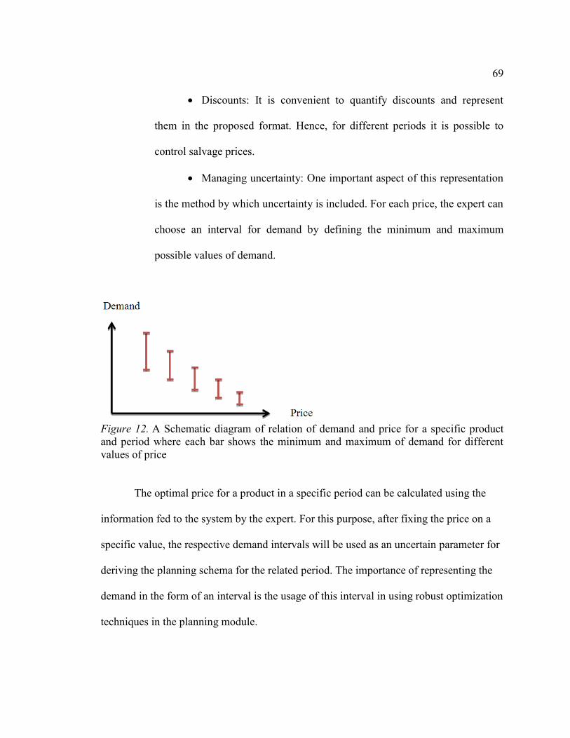
69

Discounts: It is convenient to quantify discounts and represent

them in the proposed format. Hence, for different periods it is possible to

control salvage prices.

Managing uncertainty: One important aspect of this representation

is the method by which uncertainty is included. For each price, the expert can

choose an interval for demand by defining the minimum and maximum

possible values of demand.

Figure 12. A Schematic diagram of relation of demand and price for a specific product and period where each bar shows the minimum and maximum of demand for different values of price

The optimal price for a product in a specific period can be calculated using the

information fed to the system by the expert. For this purpose, after fixing the price on a

specific value, the respective demand intervals will be used as an uncertain parameter for

deriving the planning schema for the related period. The importance of representing the

demand in the form of an interval is the usage of this interval in using robust optimization

techniques in the planning module.

70

5.2 Processes

The main process of pricing and planning modules is to determine the optimal

price and plan of production. In practice, these two decisions are usually made separately.

However, solving these two problems simultaneously can improve the quality of

solutions.

Pricing, as one of the decisions with a high impact on the profitability of a firm,

has always been a debatable issue among researchers and practitioners. In a study

conducted by Zbaracki et al. (2004), it is shown that the cost of adjusting the price can eat

up to approximately 20% of the net margin. Other studies also show the high impact of

pricing decisions on profitability (Levy, Bergen, Dutta, & Venable, 1997; Slade, 1998).

Conventionally, the pricing decision is made by considering the marginal costs of

production. However, it can be shown that considering only marginal costs on pricing can

result in poor decisions and less profit (Robinson & Lakhani, 1975). Hence, it is essential

to determine the price of products while having a broader perspective of the firm’s

processes, such as production and inventory planning. Even using an integrated model of

planning-pricing with limited demand information can result in better decisions in terms

of profitability when compared with simple cost-based pricing (R. Balakrishnan &

Sivaramakrishnan, 2001).

One of the decisions heavily related to pricing is production planning (Federgruen

& Heching, 1999). There is a large body of research on simultaneous production planning

and pricing. A comprehensive review and analysis of the problem is proposed by Chan et

al. (2004). In their research, the problem of production planning and pricing is

71 categorized according to the length of horizon, dynamic of prices, demand type, demand

functional form, demand input parameters, sales, restocking, production setup cost,

capacity limits, and products.

In this research, a special case of demand type is considered in which the demand

is uncertain – with no knowledge of statistical distribution – and is cost sensitive. For

each period, multiple candidate price points with possible minimum and maximum

demands associated with it are introduced, among which a single price for each period

will be chosen. This type of price-demand definition is very useful when there is not

enough information about the reaction of the market to different prices and/or the

decision maker just wants to examine a limited set of prices. This method of price-

demand definition is also very practical in terms of modeling where a product needs to be

sold with a lower price after a certain time. By this approach, the sales expert or decision

maker has a lot of flexibility in terms of modeling the different patterns of price-demand

and can take various factors into consideration such as seasonality, competition, and

demand sensitivity without knowing the distribution of the demand. A robust

optimization approach will be applied to incorporate this type of demand and the

“unconscious search” (Ardjmand & Amin-Naseri, 2012) metaheuristic will be used as the

solution method. So far there have been several research papers released in the domain of

simultaneous pricing and planning.

Kunreuther and Schrage (1973) modeled the problem of joint planning and

pricing with a single product, multi-period setting–for each order processed, there was a

fixed cost associated. In their research, the demand is considered to have a deterministic

72 curve in each period. They proposed a fast-converging algorithm for solving the problem,

taking into consideration a fixed price for the product in each period. However, they

suggested that using a variable pricing policy could increase the profitability.

Federgruen and Heching (1999) addressed the problem of single product, multi-

period joint pricing and inventory replenishment under demand uncertainty, where the

demand is a function of price. In their model, sellouts were considered to be backlogged.

They solved the problem in two cases, using a finite and infinite number of periods and

proposing a value iteration method. In addition to their basic model, they also analyzed

the effect of lead times, price change bounds, and order size on the problem.

Gilbert (1999) proposed a model for the planning and pricing of a single product

with seasonal demand, where the proportion of demand values in different periods are

independent of prices and there is a fixed setup cost associated with each period. He

developed a procedure for solving the problem which was capable of obtaining the

optimal solution.

Balakrishnan and Sivaramkrishnan (2001) considered the problem of planning

and pricing in a hierarchical setting, where pricing and planning would be done in two

separate phases and the solution could be revised when extra information about demand

became available. Gox (2002) considered the planning and pricing problems of a

monopolist with uncertain demand. He modeled two types of capacity constraints--

namely soft and hard, where which soft constraints could be violated at a cost, but hard

ones could not be violated.

73

Geunes et al. (2006) proposed a model for planning and pricing in the presence of

order selection flexibility. They considered a single-period model where the demand

could change with price. In their model, the production capacity was considered

unlimited. Smith et al. (2009) formulated a single product, joint planning and pricing

problem with capacity and inventory constraints. Their solution process consisted of two

steps. In the first step, they solved the single-period problem in a precise manner, and in

the second step they used this solution to solve the multi-period problem by dynamic

programming.

Chen and Hu (2012) addressed the joint inventory planning and pricing problem,

where the demand was deterministic and the cost of adjusting the price was high. They

proposed a polynomial time algorithm as the solution method, which worked based upon

the longest path problem in graphs. Mardaneh and Cacceta (2013) proposed the problem

of planning and pricing in a multi-period and multi-product setting with backorders. They

formulated the problem in terms of non-linear programming and proposed a method of

solution for calculating the optimal price and production amount in a finite time horizon.

Chen et al. (2014) proposed a model for the situation where two types of make-to-order

and make-to-stock products were produced and the demand was price-sensitive. In their

model, the excess demand was backlogged or lost.

In the literature, when the demand is considered to be price-sensitive, it is usually

assumed that if the price is known, then the demand can be determined. In reality, even

when one knows the price, there can still be a lot of deviation in demand. Additionally, in

many cases it is not possible to determine a function which relates the demand to price,

74 so in these cases only a few different options for price are available. The reasons behind

this research are the uncertainty of the demand when even the price is determined, as well

as the complexity of estimating the price-demand function.

In this research, for solving the problem of simultaneous pricing and planning, a

joint production planning and pricing model in a multi-product and multi-period setting is

proposed. The demand is considered to be price-sensitive and uncertain, while only a few

price-demand estimations are available for each product in each period. For each price it

is possible to determine the minimum and maximum demand occurring. In order to

immunize the solution against demand variations, a robust mathematical model is

proposed. In section ‎5.2.1, a brief introduction to robust optimization is given, and then in

sections ‎5.2.2, ‎5.2.3, and ‎5.2.4, the mathematical model used in the pricing and planning

module is explained.

5.2.1 Robust Optimization

A robust optimization problem is defined as follows. Considering the

optimization problem of the form { }, define as the set of uncertain

parameters in row of the matrix . Each member of the th row of the matrix , namely

, where , can be modeled as a random variable belonging to [

]. can be defined as

. Obviously, [ ].

The first formulation of robust linear optimization was introduced by Soyster

(1973), and is as follows.

75

∑

∑

∑

(1)

In this formulation, all the uncertain parameters are set to their worst case value.

Although this type of modeling obtains a good solution for all the realizations of

uncertain data, the value of the objective function can be significantly far from the

original optimization problem. To overcome the problem of the output being too

conservative in Soyster’s formulation, another method was introduced by Ben-Tal and

Nemirovski (1998, 1999, 2000). However, in their formulation, potential computational

tractability was a problem. To overcome the problem of the non-linearity and

conservatism of the methods proposed Soyster and Ben-Tal and Nemirovski, Bertismas

and Sim (2003, 2004) reformulated the model (1) in the following format.

∑

∑

∑

(2)

76

Where is the maximum number of uncertain parameters in constraint , and

and are the dual auxiliary variables which are used to guarantee the linearity of the

model. Model (2) is a generalized form of model (1). In fact, if , models (2), (1)

will be equal. Please note that ∑ | | .

According to Bertismas and Sim (2004), it is unlikely that all the have the

worst possible value at the same time, and hence it seems more realistic to define a

maximum number of uncertain parameters that may have the worst case value.

demonstrates the protection level against the worst-case realization of uncertain

parameters.

With this brief introduction into robust optimization, in the next section a

mathematical model for simultaneous pricing and planning will be introduced, and in

later sections a robust counterpart for it will be proposed.

5.2.2 Non-linear Model

The notation used in this research is as follows.

Parameters:

Holding cost of product per period

Production cost of product per unit

Lost sale cost of product per unit

th possible price of product in period

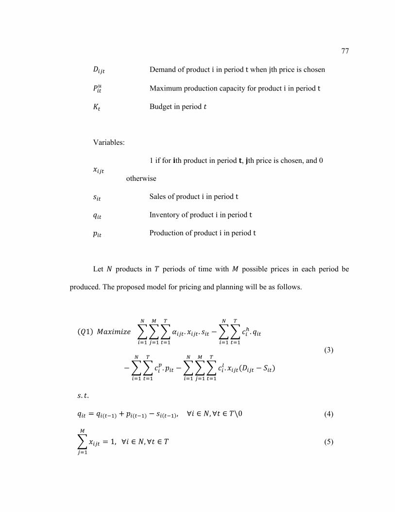
77

Demand of product in period when th price is chosen

Maximum production capacity for product in period

Budget in period

Variables:

1 if for th product in period , th price is chosen, and 0

otherwise

Sales of product in period

Inventory of product in period

Production of product in period

Let products in periods of time with possible prices in each period be

produced. The proposed model for pricing and planning will be as follows.

∑∑∑

∑∑

∑∑

∑∑∑

(3)

(4)

∑

(5)

78

∑

(6)

∑

(7)

(8)

(9)

{ } (10)

The objective function maximizes profit by subtracting the inventory, production,

and lost sale cost from sales. Constraint (4) is the inventory balance between inventory

level, production, and sales. Constraint (5) guarantees that only one price for a product in

each time period is chosen. Constraint (6) limits the maximum sales amount to demand,

while constraint (7) assures the production budget does not exceed the maximum in each

time period. Constraint (8) sets an upper bound for each product in each time period, and

finally, constraint (9) bounds the production, sales, and inventory to positive integer

numbers.

5.2.3 Linear Model

In problem (Q1), the demand is considered to have deterministic values for each

possible price. However, it would be more realistic if the demand was considered to be a

random variable belonging to an interval. To reformulate the (Q1) with demand

uncertainties, the format of model (2) will be followed. However, since (Q1) is nonlinear,

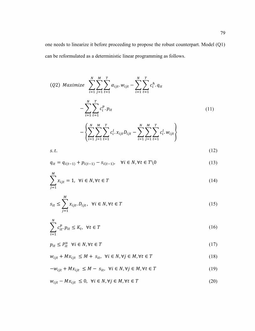
79 one needs to linearize it before proceeding to propose the robust counterpart. Model (Q1)

can be reformulated as a deterministic linear programming as follows.

∑∑∑

∑∑

∑∑

{∑∑∑

∑∑∑

}

(11)

(12)

(13)

∑

(14)

∑

(15)

∑

(16)

(17)

(18)

(19)

(20)

80

{ } (21)

(22)

in which and is a very large positive integer. Note that adding

constraints (17-19) and introducing the new decision variable convert (Q1) into a

linear problem (Q2).

5.2.4 Robust Model

As it is shown in Q2, the uncertain demand ( ) appears in the objective function

coefficients and constraint coefficient as well. In order to simplify modeling the robust

counterpart of Q2, it is possible to substitute ∑ ∑ ∑

in the objective

function and add ∑ ∑ ∑

to the model as constraint.

In order to write the robust counterpart corresponding to the constraints involving

uncertain parameters, first the protection function needs to be written, then the robust

counterpart of Q2 can be concluded from the latter functions. Thus, model (24) is the

mentioned protection function where is the set of that (

{ | }), and is the budget uncertainty.

∑

∑

81

Moreover, the protection function corresponds to constraint (15) for a given and

is defined in model below where is the set of , that are subject to

uncertainty, and is the budget of uncertainty corresponds to constraint (15).

∑

∑

The robust counterpart of the problem (Q2) can be written as follows.

∑∑∑

∑∑

∑∑

∑ ∑ ∑

(23)

(24)

(25)

∑

(26)

∑

(27)

∑∑∑

∑

(28)

82

(29)

∑ ( )

∑

(30)

(31)

(32)

(33)

(34)

{ } (35)

(36)

(37)

where , , , and are dual variables defined for the abovementioned protection

functions. It is important to note that in the abovementioned model, there is uncertain

demand appearing in two different constraints with two budget on uncertainties, and

that both of them are related to the number of uncertain demand to their

corresponding constraints. Thus, there is a linear dependency between these two budget

of uncertainties, i.e., it is ∑ ∑

.

5.2.5 Solution Methods

For solving the proposed robust optimization problem, two methods are used in

this research. The first method is using CPLEX Optimization Studio 12.3, which applies

an exact method. Although this method gives an exact solution, for large instances it may

take a very long time to find the optimum solution. The second solution method used is

83 unconscious search (US). US is a multi-start, memory-based metaheuristic that mimics

the process of psychoanalytic psychotherapy. In the next two sections, solution methods

will be explained in more detail.

5.2.5.1 Exact Method

The exact method used for solving the problem of simultaneous pricing and

planning is using CPLEX Optimization Studio 12.3. The CPLEX code used in the pricing

and planning module can be found in appendix A. Although the CPLEX yields the exact

solution for this problem, but as the dimension grows, it becomes more and more time

consuming to solve it by using CPLEX. Thus, it may not be the best method for real life

problems. For this reason, an unconscious search algorithm is proposed for solving this

problem.

5.2.5.2 Unconscious Search

Unconscious search is a metaheuristic algorithm. “Metaheuristics, in their original

definition, are solution methods that orchestrate an interaction between local

improvement procedures and higher level strategies to create a process capable of

escaping from local optima and performing a robust search of a solution space” (Fred

Glover & Kochenberger, 2003). This approach in metaheuristics consists of transcribing

the tendency in a natural phenomenon towards improvement in mathematical symbols

and codes, as well as reducing the problem-solving operations into an algorithm that

consistently traces the dynamics of that metaphorically deployed phenomenon. Some of

the most well-known metaheuristics include Genetic Algorithm (Goldberg, 1989;

Holland, 1975), Simulated Annealing (Kirkpatrick, Gelatt, & Vecchi, 1983), Tabu Search

84 (F. Glover, 1989, 1990), Ant Colony (Dorigo, Maniezzo, & Colorni, 1996), and Particle

Swarm Optimization (Kennedy & Eberhart, 1995).

Since the original conceptualization that led to the development of metaheuristics

and the inspired deployment of the probabilistic process entailed in “Survival of the

Fittest” as proposed by the Darwinian Theory of Evolution, further research has led to

analogies with systems in new domains. The common thread running through all these is

the set of rules by which the state of the domain undergoes a shift towards improvement.

Among these, the most unexplored areas are by far psychology and psychoanalysis (F.

Glover, 2007). Possessed of an integrated and united set of rules--which together improve

the mental state of a patient-- psychoanalysis appears to offer a very promising metaphor

in the area of optimization research. The unconscious search (US) metaheuristic, a

method based on the analogy between concepts used in the psychoanalytic psychotherapy

procedure and those in optimization problems, is used for solving simultaneous pricing

and planning in this research.

Unconscious search is a multi-start, memory-based metaheuristic that mimics the

process of psychoanalytic psychotherapy proposed by Sigmund Freud, where the

therapist tries to find the root cause of a patient’s mental disorder in his/her unconscious

(Freud, 1913, 1975a, 1975b, 1993a, 1993b). In psychoanalysis, it is assumed that the

cause of a mental disorder is lodged in the unconscious mind of the patient, and if the

patient can remember that – i.e. make it conscious – his/her mental disorder will be

resolved. However, the unconscious thoughts resist being revealed, and it is the job of the

psychoanalyst to help the patient gain access to them by helping him/her overcome the

85 resistances. The most common patterns of resistance encountered during psychoanalysis

are “displacement” and “condensation”. Displacement is the diversion of attention

through substituting a signifier in a patient’s talk with another one that hides the

unconscious better. Condensation is a type of resistance in which two or more signifiers

in a patient’s talk are “condensed” into one symbol in order to hide the unconscious

contents. In order to overcome the displacement and condensation resistances, the

psychoanalyst tries to guide the patient what to start talking about and in which direction

he/she should continue his/her talk. In other words, the psychoanalyst shows the patient

the path to his/her unconscious based on their observations so far, and the patient tries to

search more in depth on the path shown to him by the psychoanalyst.

Similarly, in an optimization problem the optimal answer is not already known,

and in order to reach the optimum, one needs to overcome the resistances of the search

space, which are in the form of local optimums. For this purpose, it is very important to

know where to start and in which direction to move.

Unconscious search uses the same principle for finding the optimum solution. In

each step, US maintains a list of the best found solutions and tries to find a good starting

point and direction for searching by using these solutions and memorizing the starting

points and directions that led to finding these solutions. For this purpose, US uses two

types of memory, namely “displacement” and “condensational” memories. Displacement

memory memorizes the most promising areas for the starting point, while condensational

memory memorizes the most promising directions for searching. Whenever US finds a

good solution, it tries to improve it further by using a local search.

86

US has been used in various optimization problems so far (Amin-Naseri,

Ardjmand, & Weckman, 2013; Ardjmand & Amin-Naseri, 2012; Ardjmand, Park,

Weckman, & Amin-Naseri, 2014). To explain the details of US, consider the following

optimization problem1.

The objective function may be linear or nonlinear. Functions and

are constraints of vector , where is the set of decision variables, and condition

restricts the components of to a range of values. For solving optimization

problem , initially, a set of feasible solutions ( ) is generated.

is the size of the measurement matrix in which the sorted set of the best

feasible solutions, i.e. those nearest to the optimum solution that are visited during the

search process, are held. can be defined as follows:

{ ( ) ( ) } (38)

The solutions kept in are used to measure the resistance, and are ranked by

means of a “translation function” according to the value of said resistance. The

translation function maps the value of the objective function of any solution (i.e. a

solution that belongs to ) into a range for where . 1 - Note that the notations used for explaining unconscious search is independent of the rest of this research and belongs only in this section.

87

Any solution that does not belong to and an objective function that is greater

in value than the worst solution within is assigned a scalar penalty value .

The translation function is defined as follows:

( ( ))

( ( )) (39)

In (39) above, is a sigmoid function and is used to calculate the proximity of

solutions in to the optimum solution (i.e. “unconscious” Λ { }, see

Figure 1). and are the parameters of and are calculated in every iteration in the

course of this search.

Figure 13 is a plot of the translation function against the values of the objective

function for the members of the measurement matrix. As can be seen from the graph, the

best member of the measurement matrix is assigned the value , while the

worst member is assigned the value by the translation function. For any solution

that lies outside the measurement matrix for which the objective function is greater in

value than the worst solution within , there is a penalty value assigned to that

solution. Note that in minimization problems, ( ) and

( ) . Conversely, in maximization problems we have

( ) and ( ) .

88

Figure 13. Translation function and measurement matrix

Evaluating the resistance level in solutions is performed by means of the

translation function and by the displacement and condensational memories.

measures the quality of the solutions, while the displacement and condensational

memories memorize the resistance patterns in the solutions. The displacement memory,

shown by , memorizes the displacement pattern of resistance in the solutions, i.e.

dividing the possible range – considering that – of every solution component into

equal parts. It then assigns the output of ( ) to the corresponding part. In other

words, determines how much resistance will occur if a specified range of is assigned

to solution component .

can be defined as follows:

{( ) } (40)

in which,

89

{ } (41)

{ } (42)

and is the number of decision variables. and

are defined as follows:

(∑ ( ( ))

)

(43)

∑ for solutions with an objective function

greater than the worst solution in

(44)

in which { } is the Memory Size that shows the last performed iterations

of algorithm that are memorized. represents the jth subinterval of . As we increase

the value of the parameter , the effect of those lower quality solutions encountered in

the previous iterations on determining the search path becomes more apparent. Increasing

has the advantage that it causes diversification to increase; on the downside, it could

lengthen the time spent on searching. (To make this point clearer, compare it with the

metaphor of psychoanalysis: as the psychoanalyst gets closer to the unconscious,

associations made by the subject become more representative of the contents of the

90 unconscious, and hence are more important to the psychoanalyst.) is the worst

solution in , and is the value of the th decision variable in solution .

By means of the displacement memory , a new solution can be constructed. This

solution is denoted by . The th solution component will be assigned to one of

the possible ranges in solution space, with a probability defined as follows:

{ }

( )

∑

( )

(45)

in which is the probability function and is a predefined constant. When the

solution component is assigned to , it will choose a number in at random. The

larger the value of , the more the probability of ; the larger the value of

,

the less the probability of .

Once a displacement-free solution (DFS) has been reached, the condensational

memory is used to eliminate the condensational resistance pattern. Displacement

memory is used for constructing a new displacement-free solution (DFS), while

condensational memory is used to improve the solution constructed with the help of ,

making it a condensation-free solution (CFS).

Condensational memory is defined as follows:

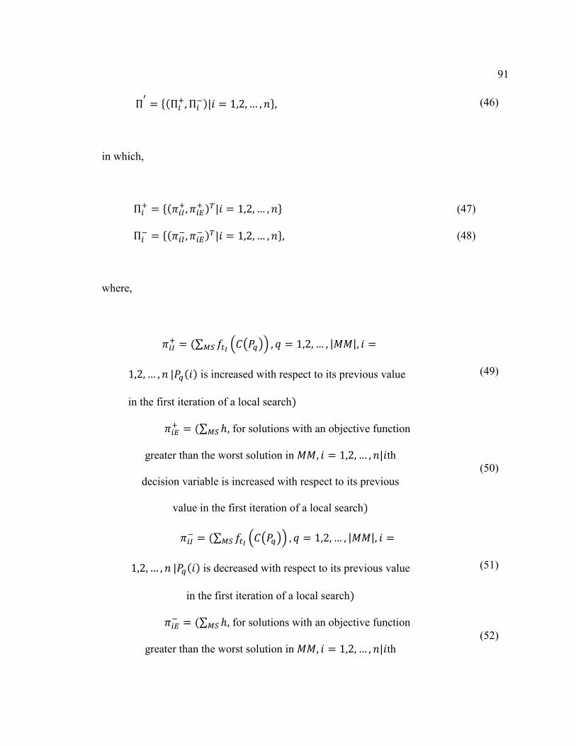
91

{

} (46)

in which,

{

} (47)

{

} (48)

where,

∑ ( ( ))

is increased with respect to its previous value

in the first iteration of a local search

(49)


greater than the worst solution in th

decision variable is increased with respect to its previous

value in the first iteration of a local search

(50)

∑ ( ( ))

is decreased with respect to its previous value

in the first iteration of a local search

(51)


greater than the worst solution in th (52)

92

decision variable is decreased with respect to its previous

value in the first iteration of a local search

Note that, since in the beginning of the first iteration of US, we do not perform a

local search, we do not have any information with which to update ; thus, equations

9~15 are applied from the second iteration onwards.

Once is constructed, determines whether is to be decreased or

increased by calculating two values

and

and generating a random

number 𝜓 in the range

. If 𝜓 , the value of will be increased by as

much as a predefined number δ { }; otherwise, the value of will be

decreased by the same amount δ. Decreasing or increasing the value of will be

repeated until the limits of are reached, as long as the solution still remains feasible.

Having constructed , the first solution in an iteration is known as the “mother

solution”. By using memory , solutions , , … are generated from . Solution is

the DFS, while solutions , , … are CFSs derived from the mother solution . The

best solution among , , , …, called ,will be the starting point in the local search.

Memories and help to appoint the region where the mother solution should

be located and the direction along which the mother solution is to be moved, by

increments of δ, in order for the solutions , , … to be generated. The functions of

these two memories for the situation where there are two decision variables and are

shown in Figure 14.

93

Figure 14. Functions of 𝚷and 𝚷 for the situation where there are two decision variables, and

After obtaining the solution , a local search is conducted with as the starting

point. If the result of the search is , it is obvious that . In the process of

reaching , more resistance patterns are revealed, and and are updated by the use of

. Notice that will be updated only if the objective function value of is better

than the objective function value of , in which case will be updated so that the

following inequality holds:

(53)

in which and are the members of before is augmented. In order for

the above inequality to always hold, should remain sorted through every update. If

is changed, the function must be corrected to match the new , i.e. the

coefficients and must be adjusted. Denoting the new coefficients by and , as well

as the best and the worst solutions in by and , we will have:

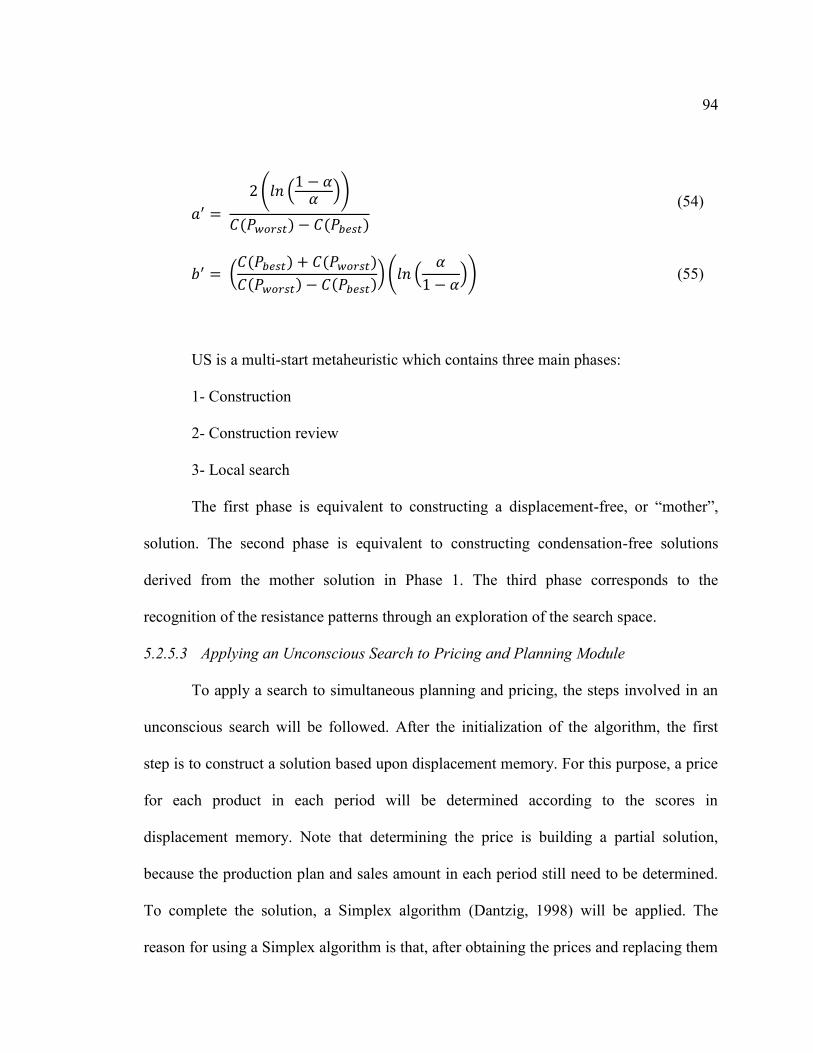
94

( (

))

(54)

(

) ( (

)) (55)

US is a multi-start metaheuristic which contains three main phases:

1- Construction

2- Construction review

3- Local search

The first phase is equivalent to constructing a displacement-free, or “mother”,

solution. The second phase is equivalent to constructing condensation-free solutions

derived from the mother solution in Phase 1. The third phase corresponds to the

recognition of the resistance patterns through an exploration of the search space.

5.2.5.3 Applying an Unconscious Search to Pricing and Planning Module

To apply a search to simultaneous planning and pricing, the steps involved in an

unconscious search will be followed. After the initialization of the algorithm, the first

step is to construct a solution based upon displacement memory. For this purpose, a price

for each product in each period will be determined according to the scores in

displacement memory. Note that determining the price is building a partial solution,

because the production plan and sales amount in each period still need to be determined.

To complete the solution, a Simplex algorithm (Dantzig, 1998) will be applied. The

reason for using a Simplex algorithm is that, after obtaining the prices and replacing them

95 in the model, no binary decision variable remains in the model, and it thus turns into a

linear model without any binary variables. Solving this linear model with a Simplex

model is very easy and possible in polynomial time. The Simplex C++ code used can be

found in appendix B (Moreau, 2009).

After the partial solution generated by an unconscious search is completed by

using a Simplex algorithm, the second step of US--construction review--is started. In this

step, the prices of products in each period are increased or decreased based upon the

condensational memory. After each change in price, a Simplex algorithm is used to

complete the solution. Finally, after the construction review step, a local search is

conducted to improve the solutions. In a local search, a random price for a product in a

random time period is picked and changed. If the results improve, the change will be

accepted; otherwise, it will be rejected, and another product or period will be picked. This

procedure continues until no further improvement is possible. Figure 15 shows the flow

chart of applying an unconscious search to the problem of simultaneous pricing and

planning.

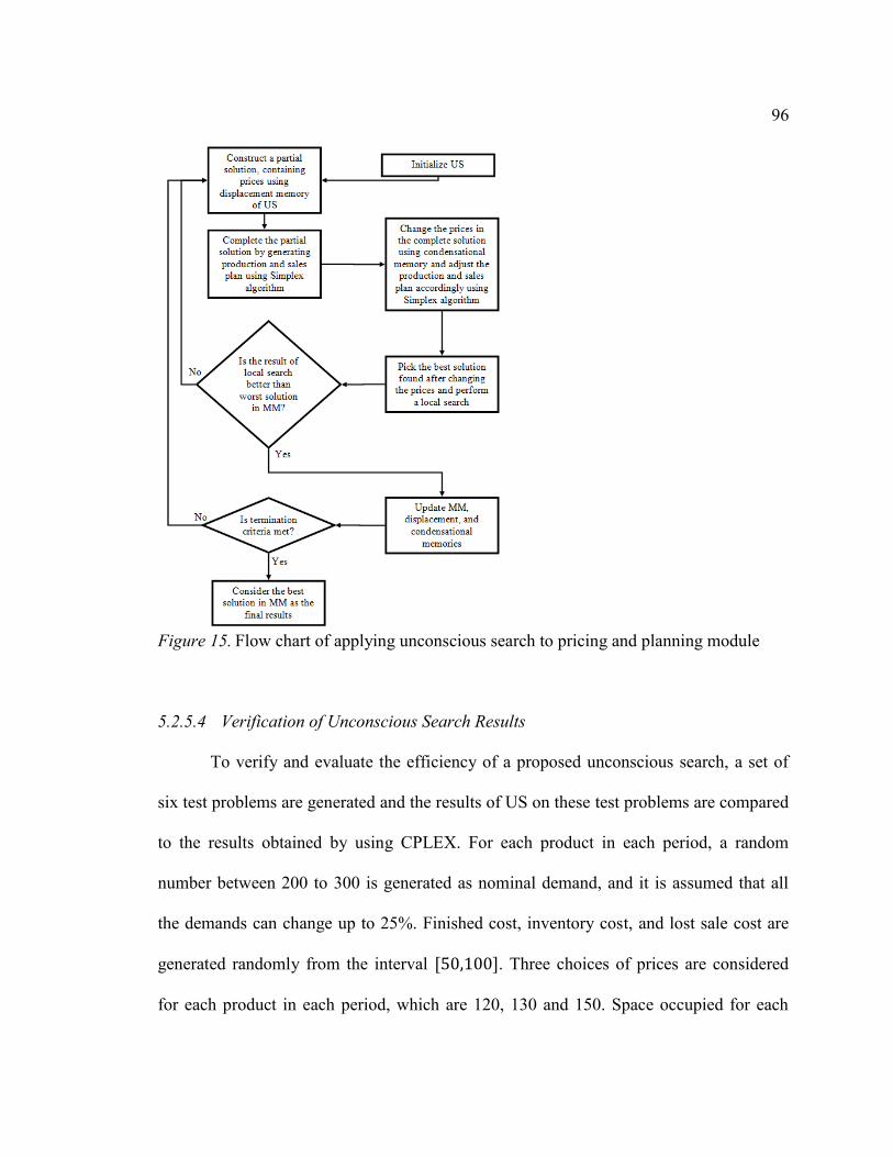
96

Figure 15. Flow chart of applying unconscious search to pricing and planning module

5.2.5.4 Verification of Unconscious Search Results

To verify and evaluate the efficiency of a proposed unconscious search, a set of

six test problems are generated and the results of US on these test problems are compared

to the results obtained by using CPLEX. For each product in each period, a random

number between 200 to 300 is generated as nominal demand, and it is assumed that all

the demands can change up to 25%. Finished cost, inventory cost, and lost sale cost are

generated randomly from the interval [ ]. Three choices of prices are considered

for each product in each period, which are 120, 130 and 150. Space occupied for each

97 product is considered to be 2, while the warehouse and budget capacity for each period

are fixed at 5000 and 50000, respectively. The maximum production number for each

product in each period is set to 700. Table 10 lists the six test problems’ specifications,

including the number of periods and products in each.

Table 10: Test problems’ specifications used for evaluation of unconscious search Test Problem No. of Periods No. of Products

1 1 4

2 1 4

3 2 5

4 2 5

5 4 10

6 4 10

Table 11 lists the results of the exact and US algorithms applied to the six

randomly generated test problems. Each test problem is solved by US ten times, and the

best and worst results obtained are reported. As it can be observed, US has been able to

find the optimum solution in a very short time compared to the exact method. The time

gap between the two algorithms is even more evident as the dimension of the problem

increases. The results obtained show the efficiency and quality of US for solving joint

pricing and planning problems. Note that in test problems 5 and 6, the value of the

objective function is negative, due to budget constraints and the high number of lost

sales.

98

Table 11: Solution quality and run time of exact and US algorithms for six artificially

generated test problems; for each instance, US has run 10 times

Test

Problems

Exact Method Unconscious Search

Exact solution Time (s) Best Solution Worst Solution Time (s)

1 37005 2.94 37005 37005 0

2 49540 1.95 49540 49540 0

3 31364 2.43 31364 31364 0

4 95980 2.43 95980 95980 0

5 -169216 15.85 -169216 -169216 0

6 -92622 19.67 -92622 -92622 0

5.3 Design and Outputs of Pricing and Planning Module

The pricing and planning module has two outputs. The first output is the price for

each product in each period, and the second output is the production and sales plan for

each product and period. Figure 16 shows a prototype of a pricing and planning interface,

where the specifications of each product and period, as well as the constraints, can be

adjusted. The inputs from finance and cost estimation modules will be loaded into the

interface automatically.

99

Figure 16. A prototype of pricing and planning interface

Figure 17 depicts the inputs, processes, and outputs of the pricing and planning

module.

Figure 17. Inputs, processes and outputs of the pricing and planning module

100

6 SCHEDULING MODULE

The third module of proposed decision support system is scheduling. A

scheduling module, having a production and sales plan as an input, schedules a plan

calculated by a pricing and planning module in each time period. For this purpose, in

addition to scheduling the products on stations, it is necessary to control the progress of

jobs at hand. Hence, there are two main processes in a scheduling module. The first

process is scheduling the tasks, and the second one is controlling the progress of

scheduling and to make corrections if necessary. In this chapter, the inputs, processes,

and outputs of a scheduling module are introduced.

6.1 Inputs

The first set of inputs to a scheduling module, which is the production plan,

comes from the pricing and planning module. In addition to a production plan, the

available times and production specifications--such as flow process charts, machines, and

the skill level of operators--are the other inputs of a scheduling module. These inputs will

be discussed in detail in the following sections.

6.1.1 Inputs from Pricing and Planning Module

The first input of a scheduling module is the production plan generated in a

pricing and planning module. A production plan consists of a product, the number of its

production in a time period, and the length of the period. As an example, if a pricing and

planning module has determined 200 as the number to produce in period , then the

scheduling module will receive this input as a task that needs to be scheduled, while its

release time and deadline are the beginning and ending of period , respectively. Hence,

101 the output of the pricing and planning module will be introduced to the scheduling

module in the form of jobs. Each job has several attributes. These attributes include the

product, number of production, release time, deadline, priority, and the delay between

different stages of production. The delay between production stages is the time that

should pass until an activity can be started after all its predecessors have been scheduled.

6.1.2 Timeline and Working Hours

In order to schedule the tasks, it is necessary to know the working and non-

working hours, break times, and number of working shifts for each day. All these

specifications of a timeline will be called a work profile. A work profile has various

attributes by which time colander and available times can be defined. An example of a

database designed for recording profiles can be found in appendix C. Different working

profiles can be defined for the system and used according to need. In scheduling, only

allowed times obtained from work profiles will be used for calculations. Note that,

although the constraint imposed by work profiles may increase the complexity of

scheduling dramatically, but it is necessary to consider all these constraints in order to

have a realistic scheduling setting.

6.1.3 Machines

Machines are the processing units of scheduling problems by which a product is

processed. In this research, any processing tool is considered to be a machine. A

machine’s performance is an indicator of how reliable that machine is in finishing a job

on time. The performance of a machine in this research is evaluated by using “Overall

Equipment Effectiveness” (OEE). OEE is the lean time that a machine properly works. In

102 calculating the OEE, only the time that a machine is working without being interrupted or

producing defective products is considered. Figure 18 indicates how the OEE can be

calculated after subtracting from the scheduled time the repair and inefficient times plus

the times a machine is producing a defective product. Repair time is the time that a

machine needs immediate attention due to an unexpected stoppage or interruption in the

production process, while inefficient time is the time that a machine loses due to

variations in standard cycle times.

OEE is a very comprehensive measurement criterion in terms of evaluating the

efficiency of production lines (Dal, Tugwell, & Greatbanks, 2000; Godfrey, 2002;

Muchiri & Pintelon, 2008). In this research, OEE will be used to determine and modify

the total numbers of production needed on a machine. As an instance, if 200 units of a

product is to be produced on a machine and the machine’s OEE is 0.9, it makes more

sense to schedule

units for that machine. The extra 22 units are due to the

various inefficiencies that the machine has.

Figure 18. The lean time remains after subtracting the repair and inefficient times plus the amount of time a machine is producing defective products

103

6.1.4 Maintenance

Having the machines as inputs, it is necessary to know the maintenance time

associate with each of them. Maintenance is important because it can make a machine

unavailable for some time intervals, and hence affect the scheduling. A machine may

have various types of maintenance for each of its parts. To track the maintenance times,

all parts of a machine need to be defined and their maintenance time recorded. An

instance of a database designed for tracking the maintenance can be found in appendix D.

6.1.5 Stations

A station involves set machines and operators that altogether work towards

assembling or producing a part or a stage of a product in its production path. Note that a

station can have one or several machines as its content. Definition of a station is

necessary because sometimes it is more convenient to define the stages of production for

a product in the form of stations. Note that each product can have different activities

performed on each station.

6.1.6 Setup Times

Each product may have different warm up or setup times on different stations.

These times can also be dependent on the product that it had just been producing. The

setup times of products on each station is defined in the form a matrix in which each

component corresponding to row and column shows the setup time for changing from

product to product . To formulate the scheduling module more realistically, the setup

time of each product is considered to have two parts, variant and invariant. The variant

104 part can be different depending upon the prior product, while the invariant part is fixed

for each product.

6.1.7 Operators and Skill Levels

Operators and their relative skill levels for producing different products are the

inputs of a scheduling module. For assessing the skill level of each operator in

association with the various activities involved in producing a product, a visual ILUO

method is used. In an ILUO method, the skill level of each operator is categorized in four

categories of I, L, U, and O, in which I is the least and O is the most skilled level

(Graham & Clare, 2007; Handyside, 1997). Note that in an ILUO method the skill level

has different parameters, such as meeting quantity, quality, and safety standards. In the

proposed decision support system, the skill level of each operator is determined by the

user.

6.1.8 Operation Chart

An operation chart (OC) is an essential input for a scheduling module. In an OC,

the production stages of a product, along with the various activities involved and cycle

times, are included. In flow shop and job shop problems, a product is supposed to go

through several stages in a linear fashion to yield a final product. However, in reality, in

producing one unit it is necessary to have a network of stages and stations that altogether

form an OC for a product. In this regard, an OC is similar to the networks used in project

management. Figure 19 depicts a prototype of an OC for a product consisting of six

stages/stations. Each rectangular shape shows a stage or station of production.

105

Figure 19. A prototype of an operation chart consisting of six stages

6.2 Processes

A scheduling module has two main processes. The first process is scheduling the

jobs. A job can be the output of a pricing and planning module, or a single job defined

separately by a user. It is even possible to consider a part of a product’s operation chart as

a job and schedule it. In total, any set of tasks that needs to be scheduled can be

considered as a job. The only constraint is that these tasks need to be related to

production. For instance, scheduling module cannot schedule a maintenance task.

The second process of a scheduling module is controlling how the progress of a

schedule is monitored and, if there is any deviation, how it will be reported to the user.

The control process helps to correct the schedule if necessary, and can also be a great

experience accumulation source by finding possible failure modes of a production line. In

the following sections, scheduling and control processes are explained in more detail.

106

6.2.1 Scheduling

Generally speaking, the goal of scheduling is to arrange and sequence the jobs on

different machines in order to optimize the resources’ consumption (Pinedo, 2012). The

setting considered for a scheduling module of the proposed decision support system is a

general setting in which most of the scheduling problem attributes are present.

In literature, among the standard scheduling problems, flexible job shop problems

are the most complex ones. Flexible job shop problems are a generalization of job shop

problems in which each an operation can be processed by a set of allowed machines.

However, the environment set for a scheduling module is more general compared to a

flexible job shop. In a flexible job shop, each job consists of a chain of operations in

which each operation can be handled on several parallel machines. In the proposed

decision support system, each job has several operations arranged in a network instead of

a chain. Hence, the problem is a combination of project and flexible job shop scheduling.

In addition to the scheduling environment, other attributes of the proposed

scheduling module are also considered to be general as much as possible. The release

dates of jobs are considered to be non-zero, which can increase the complexity of the

problem. Setup times are sequence-dependent, and hence, each sequence of the jobs may

yield a different setup time. Jobs can be broken down into two or more parts. Some parts

of the timeline are blocked, and hence it is not possible to use them in scheduling. A good

example of blocked times are the holidays, where no job should be scheduled.

The objective of scheduling problems is considered to be the minimization of

weighted tardiness, which is one of the most complex objectives in scheduling literature

107 (Pinedo, 2012). This objective is necessary because, after defining the production plan in

a pricing and planning module, the scheduling module has to guarantee that planning

output is feasible in the designated time window. The objective function needs to be

weighted because the system user may set different weights for jobs due to their

importance for customers or any other requirements necessary.

In addition, as mentioned in section ‎6.1.3, each machine has an effectiveness

measured by the OEE. The OEE of the machines can affect the scheduling problem.

Hence, it is necessary to take the OEE into consideration. For this purpose, the

completion time of each task or operation on a machine cannot be deterministic, and

needs to be treated as a stochastic parameter which is directly related to the OEE. As an

example, if the completion time of a task on a machine is 1 hour in an ideal situation and

the machine’s OEE is 50%, then the processing time needs to be considered a random

variable between 1 to 1.5 hours.

Handling the scheduling problem in a general setting is a very computationally

expensive task, and in a dynamic environment such as a production line, needs to be done

in the shortest possible amount of time. In order to address this problem efficiently, it will

be divided into two parts and treated separately. At the end, the two parts will be

combined again to form a complete solution. The reason for this division is the high

complexity of the proposed scheduling problem and the fact that there is not any unique

procedure for dealing with the problem at hand.

To propose a heuristic algorithm for the proposed scheduling problem, it will be

divided into two parts; dispatching and simulation. In the dispatching phase, the sequence

108 of jobs will be decided. Note that the constraints--such as release tim-- are not considered

in this step. The question answered in this phase is of which job should enter the

production line first. Also, it is assumed that when a job is entered the line it can consume

all the resources necessary without taking the requirements of next job into consideration.

In this regard, the problem will be reduced to a simple travelling salesman problem

(TSP), which can be solved by a good heuristic efficiently. The heuristic used in this

research is the variable neighborhood search (VNS).

In the second phase, after determining the sequence of the jobs, the jobs need to

be scheduled separately. For this purpose, each job needs to be scheduled individually as

well. Since each job is a project with probabilistic task durations, the problem of

scheduling a single job is also a complex problem. For solving this problem, a Monte

Carlo simulation method is used, in which different values are assigned to task durations

based on the OEE of the machines.

Figure 20 shows the general framework of the heuristic used in scheduling

modules for sequencing the jobs. The process of scheduling a single job and the sequence

of the jobs will be explained in the following sections.

109

Figure 20. General framework of the heuristic used in a scheduling module

6.2.1.1 Scheduling One Job

For scheduling a sequence of jobs in the proposed decision support system, it is

necessary to schedule each one of them separately. Each job in the system is presented as

a network of tasks that are related to each other by precedence constraints. From this

perspective, scheduling a job is very similar to assigning resources in project

management problems. For a project to be done on time, it is necessary to control the

critical path’s time and resources. For a product that is considering the operations chart,

the critical path is the set of all the activities that together form the longest path from the

beginning to the end of production. Figure 21 depicts a hypothetical operations chart for a

110 product and its corresponding critical path in red. Each circle shows a station that the

product needs to meet before completion. Although it is necessary to perform all the tasks

to have the product ready, in order to guarantee the timely finish of the product, all the

tasks on the critical path need to be done on time. The red path in Figure 21 is the longest

route from the first to the last station in terms of processing time. In this example, to

finish the project on time, it is necessary to control the times for the tasks 1, 3, 5, and 7.

Figure 21. A product’s operation chart and its critical path

Using the logic of critical path method, it is possible to schedule a job by

assigning the necessary resources to its critical path first. However, due to the stochastic

nature of the processing times, a critical path may not always stay critical. Depending on

the task durations of a product’s operations chart, there may be different critical paths. To

find different possible critical paths, a Monte Carlo simulation is performed. In the

simulation, each time a processing time is assigned to tasks, based upon the average

processing time and OEE of the machine used. Then, the critical path is determined.

Having different possible durations, a task may be part of a potential critical path. The

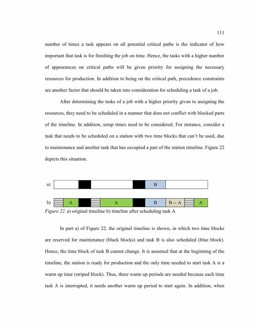
111 number of times a task appears on all potential critical paths is the indicator of how

important that task is for finishing the job on time. Hence, the tasks with a higher number

of appearances on critical paths will be given priority for assigning the necessary

resources for production. In addition to being on the critical path, precedence constraints

are another factor that should be taken into consideration for scheduling a task of a job.

After determining the tasks of a job with a higher priority given to assigning the

resources, they need to be scheduled in a manner that does not conflict with blocked parts

of the timeline. In addition, setup times need to be considered. For instance, consider a

task that needs to be scheduled on a station with two time blocks that can’t be used, due

to maintenance and another task that has occupied a part of the station timeline. Figure 22

depicts this situation.

Figure 22. a) original timeline b) timeline after scheduling task A

In part a) of Figure 22, the original timeline is shown, in which two time blocks

are reserved for maintenance (black blocks) and task B is also scheduled (blue block).

Hence, the time block of task B cannot change. It is assumed that at the beginning of the

timeline, the station is ready for production and the only time needed to start task A is a

warm up time (striped block). Thus, three warm up periods are needed because each time

task A is interrupted, it needs another warm up period to start again. In addition, when

112 one schedules task A after task B, a setup time is necessary (grey block). A good method

for scheduling jobs in a real setting needs to implement all these constraints after

determining the priority of tasks.

Figure 23 shows the flowchart of scheduling a single job. First, all the

specifications of the job are read from the database. Then, using the OEE of the machines

needed for the job and the average task’s durations, a Monte Carlo simulation is

conducted to determine the possible critical paths. Based on the number of times that a

task appears on the critical paths, the tasks are then prioritized. At the end, considering

the existing constraints on the schedule and the precedency, all the tasks are scheduled.

This procedure continues until the whole job is scheduled.

113

Figure 23. Flowchart of scheduling a single job

6.2.1.2 Optimizing Dispatching Rule Using Variable Neighborhood Search

After introducing the procedure for scheduling a single job, it is necessary to

implement all of the jobs in order to minimize the total weighted tardiness. The problem

of determining an optimum sequence for dispatching the jobs into a production line can

be interpreted as a traveling salesman problem (TSP). In TSP, the objective is to find a

Hamiltonian path in a directed or undirected graph so that the sum of weights of the

vertices on the path is minimized. Likewise, in finding the best sequence of jobs, the

objective is to find an ordered set of the jobs that include all of the jobs and, if

114 implemented in that order, minimize the total tardiness. For solving the proposed TSP, a

variable neighborhood search (VNS) is applied.

VNS is a metaheuristic which operates based upon changing the neighborhood

systematically (Hansen & Mladenović, 2003; Mladenović & Hansen, 1997). To explain

VNS, consider an optimization problem of the form { }. Let us

define as the set of neighborhood structures. Hence for a solution ,

there are solutions that are its neighbor and can be reached by the th

neighborhood structure. In basic VNS, first an initial solution s chosen. Then, having

, the neighbors of the generated solution are examined until a local optimum is

reached. In the next step, will be increased by one, and the same procedure is repeated

until a local optimum is reached. This procedure continues until all the predefined

neighbors are examined.

The same procedure can be applied to a sequence of jobs to find a good

dispatching order. For this purpose, four neighborhood structures are defined. The first

neighborhood structure can be explored by swapping two jobs in a sequence. The second

neighborhood structure can be navigated by examining three consecutive jobs in a

sequence and finding the best order for them. Using the same logic, the third and fourth

neighborhood structures are obtained by examining all permutations of four and five

consecutive jobs in a sequence. After reaching a local optimum at the end of each

neighborhood structure search, the next neighborhood structure is initiated.

Figure 24 shows the flowchart of applying VNS to finding the best sequence of

the jobs for scheduling. First, the set of neighborhood structures are defined and a random

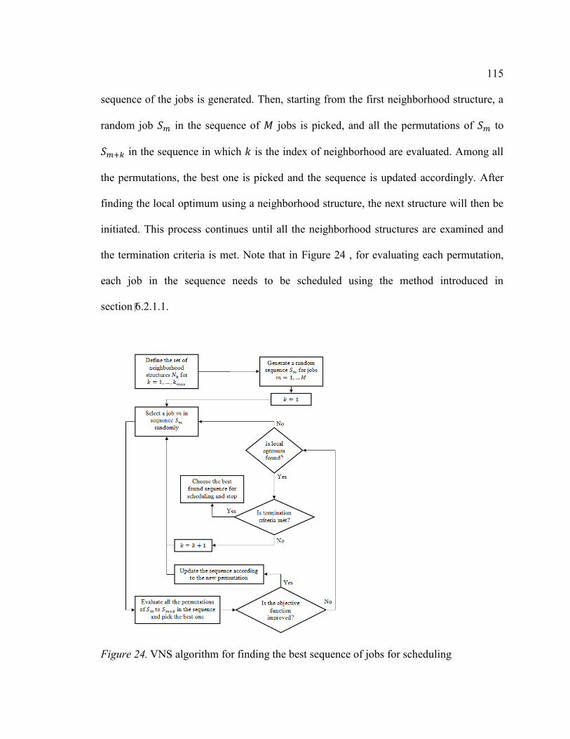
115 sequence of the jobs is generated. Then, starting from the first neighborhood structure, a

random job in the sequence of jobs is picked, and all the permutations of to

in the sequence in which is the index of neighborhood are evaluated. Among all

the permutations, the best one is picked and the sequence is updated accordingly. After

finding the local optimum using a neighborhood structure, the next structure will then be

initiated. This process continues until all the neighborhood structures are examined and

the termination criteria is met. Note that in Figure 24 , for evaluating each permutation,

each job in the sequence needs to be scheduled using the method introduced in

section ‎6.2.1.1.

Figure 24. VNS algorithm for finding the best sequence of jobs for scheduling

116

6.2.2 Control

The second process of scheduling model is “control”. This process is necessary to

make sure that the schedule is on time, and thus supports the objectives of the pricing and

planning module. The control process has two main parts. In the first part, all the

production interruption causes are recorded, while in the second phase the action plans

taken to remove these causes--along with previous knowledge in the case of the same

interruption--are recorded. To have all this data stored, it is necessary to have a database

capable of storing the data in a format that can be easily accessed.

Production interruptions can be categorized into two parts. The first group of

interruptions are those related to quality issues and production defects. For these

interruptions to be recorded, it is necessary to define the possible defect types for each

product and then, whenever an interruption of this type occurs, the reason and the action

taken are to be stored as possible action plans for future reference.

The method used for identifying and keeping track of problems and their causes is

fishbone diagram. A fishbone diagram helps to find the root cause of a problem without

using numerical and statistical approaches (Bicheno, 1998; Goetsch & Davis, 1994;

Psychogios & Priporas, 2007). In a fishbone diagram, the root cause of each problem is

considered to belong to one of the following categories: method, machine, manpower,

material, measurement, or environment.

In addition to quality problems, other types of production interruptions also need

to be monitored and their related data recorded in the database. These interruptions are

117 those related to issues such as logistics, production processes, operators, and energy

resources.

Figure 25 depicts the domain model of a control process in terms of the

scheduling module. Rectangular shapes are the entities that need to be recorded and

stored in the database. Green parts are related to quality issues, while blue parts are

related to other interruption types. Yellow parts are used for both quality and non-quality

problems. Arrows show the relation of entities to each other. For instance, a product is

connected to production-defect by an arrow, which means that each product can have

several defects related to it. In the same manner, defects are connected to product-defect,

which means that each defect type can affect several products.

One of the entities introduced in Figure 25 is “process”. A process is any kind of

activity that is taking place in production, and may include operators and machines. A

process is a part of a working station in a production line. To explain the concept of

process, consider a production line that produces raincoats. There is a station in the

production line dedicated to producing sleeves, and for sewing a sleeve, two sewing

machines are needed. One sewing machine is used for sewing the front and the other for

the back of the sleeve. In this case, sewing the front of the sleeve is a process that needs a

machine and an operator.

Using the process as a basis for monitoring the production line, it is possible to

control the line to keep the schedule on time. For monitoring the production line, two

indicators can be used--namely, overall equipment effectiveness (OEE) and parts per

million (PPM). OEE was discussed in detail in section ‎6.1.3. PPM is the number of

118 defective products in a million. The control process of a scheduling module helps to

monitor these two indicators and take quick action when they are not in a defined range.

Both of these indicators can be calculated by the database structure depicted in Figure 25.

Figure 25. Schematic domain model of the database for a control process in terms of the scheduling module

6.3 Design and Outputs of Scheduling Module

As discussed in previous sections, a scheduling module has several inputs,

processes, and outputs. Figure 26 shows the different parts of scheduling module,

including the inputs, processes, and outputs. In the input part, the rectangular shape

119 shows a module of the decision support system which feeds the scheduling module

automatically, while the other inputs are introduced into the system by a user.

The outputs of a scheduling module include a schedule, which will be used by an

inventory module, and two indicators – i.e. OEE and PPM – for monitoring the

performance of the system.

Figure 26. Inputs, processes and outputs of a scheduling module

120

7 INVENTORY MANAGEMENT MODULE

The inventory management module is the last in a series of modules for the

proposed decision support system that makes decisions based upon the outputs of the

finance and cost estimation, pricing and planning, and scheduling modules. This module

coordinates the inventory decisions in such a way as to guarantee the availability of

necessary raw materials for supporting the scheduling module. Thus, the first assumption

for an inventory management module is that no material shortage is allowed. Similar to

other modules, inventory management has a set of inputs, processes, and outputs. In the

remainder of this section, inputs, processes, and outputs of an inventory management

module will be explained.

7.1 Inputs

The inputs to an inventory management module can be divided into two groups.

The first group is those that are originated from other modules, and hence are

automatically generated. The second group is those that need to be defined by the user.

These inputs include a bill of material (BOM), as well as supplier and material

specifications. Although the automated inputs from other modules are generated

automatically, it is possible for them to be modified by the user as well. In the following

sections, these inputs will be explained in detail.

7.1.1 Inputs from Scheduling Module

The first set of inputs to an inventory management module originate from the

scheduling module. Following the decision made by the pricing and planning module, the

scheduling module arranges a sequence of the jobs in a way so as to guarantee the

121 feasibility of the plan. For a schedule to hold and be performed, it is necessary to support

it by the availability of necessary raw material at the proper time and in the proper

amount. The inventory management module receives the schedule as an input and

estimates the raw materials’ consumption based on it.

7.1.2 Inventory Holding Cost

Each raw material has a holding cost that is estimated by the finance and cost

estimation module. In the same manner that the holding cost of products was computed

by the finance and cost estimation module, it is possible to estimate the holding cost of

raw materials. The holding cost of raw materials varies based on their characteristics such

as purchase value, space occupation coefficient, and perishability.

7.1.3 Bill of Material (BOM)

To estimate the raw material consumption using a schedule of jobs, a bill of

material (BOM) is used. BOM is the set of raw material and components as well as their

needed amount for manufacturing a product. BOM is an input that needs to be defined by

the user. It is possible to have several BOMs for a product. However, only one of them is

considered to be active for planning purposes. The active BOM also needs to be defined

by the user.

7.1.4 Suppliers and Material Specifications

In addition to a BOM for each product, the specifications of the needed materials

and the set of suppliers that provide these materials need to be defined. These

specifications include: the ordering cost of a raw material to each supplier; the purchasing

price of a material from different suppliers; the minimum and maximum possible order

122 quantity for each raw material to each supplier; and the space occupation coefficient of

materials.

7.2 Processes

The main process of an inventory management module is to determine which raw

material--in what amount and to which supplier--should be ordered in order for there to

be no interruption in the schedule while minimizing the purchasing, holding, and ordering

costs. The method used for addressing this problem in this research is mathematical

modeling. Note that this problem is defined in a deterministic setting. The reason is that

the demand and a job’s processing time uncertainty is dealt with in the pricing as well as

the planning and scheduling modules. Hence, the inventory management module just

needs to support the strategy advised by the other two modules. In section ‎7.2.1, the

mathematical model for an inventory management module is proposed, which is the basis

of all decisions made in this module.

7.2.1 Mathematical Model

The following notation is used for modeling the inventory management problem.

Indices:

Material

Periods

Suppliers

Parameters:

Inventory holding cost of Material

123 Cost of ordering material from supplier

Demand of material in period

Purchasing price of material from supplier

Space occupation coefficient of material

Minimum ordering quantity of material to supplier

Maximum ordering quantity of material to supplier

A large number

Decision Variables:

Inventory level of material at the end of period

1 if material is ordered to supplier in period and 0 otherwise

Amount of material ordered to supplier in period

The mathematical model will be as follows:

∑∑

∑∑∑

∑∑∑

(56)

S.t. (57)

∑

(58)

∑

(59)

(60)

124

(61)

(62)

{ } (63)

The objective function minimizes the costs of holding inventory, ordering, and

purchasing. Note that, although shortage cost is a common assumption in inventory

models, since the inventory management module has to support the scheduling module, it

cannot have a shortage. Thus, the shortage cost is not considered for this model.

Constraint (58) is the inventory balance equation. Constraint (59) limits the inventory

level to warehouse capacity. Constraint (60) limits the ordering quantity of each raw

material to a minimum quantity. Constraint (61) makes the ordering quantity 0 if the

respective supplier is not chosen for placing an order. Constraint (62) limits the ordering

quantity to an upper bound, and constraints (63) are non-negativity and binary

constraints.

7.2.2 Solution Methods

In order to solve the proposed mathematical model for the inventory management

module, two methods will be used and compared against each other. The first method is

the exact one in which CPLEX 12.3 is used. The second method is a hybrid of a tabu

search metaheuristic and a Simplex algorithm. In the following sections these two

methods will be explained in detail.

125 7.2.2.1 Exact Solution

To solve the proposed model in an exact way, CPLEX 12.3 is used. Although the

CPLEX obtains the global optimum, due to the large scale of the problem when there are

many types of material or time periods, it becomes very time-consuming to apply CPLEX

to the problem. Hence, it is not possible to use CPLEX in real life cases of the problem.

The CPLEX code of the problem can be found in Appendix E.

7.2.2.2 Hybrid Tabu Search and Simplex Algorithm

Tabu search (TS) is a metaheuristic, which is designed to overcome local search

(LS) methods in escaping local optimums (F. Glover, 1989, 1990, 1997, 2007). Search

space and neighborhood structure are the two main concepts in TS. Search space is the

set of all possible solutions which can be reached in the course of a search. Neighborhood

structure is the type of local transformation that can be applied to a solution in order to

reach a new solution in search space. It is possible to have various neighborhood

structures in a problem.

In TS, while searching for the optimum solution, a tabu list is maintained. A tabu

list is the set of recently performed transformations that, by being repeated, may cause the

set to revisit prior solutions. A move can be tabu up to a certain number of iterations.

However, if a recently performed move can improve the solution considerably, it can be

performed. The criteria by which a recently performed move can be repeated despite

being in a tabu list is called the :aspiration criteria”. A tabu list is also known as short-

term memory (Fred Glover & Kochenberger, 2003).

126

In addition to short-term memory, another type of memory--long-term memory--

is used in TS. Long-term memory memorizes the promising domains of search space, and

helps to find a better starting point whenever the search is restarted.

A TS method will be used for solving the proposed inventory management model.

TS will be applied to the problem in order to determine if material needs to be ordered

to supplier in period or not. Thus, TS will only determine the value of the binary

variable . However, after deciding about the , the amount of material ordered

also needs to be determined. Following the model, if the values for are known, the

model will turn into a simple linear optimization problem that can be solved efficiently

using a Simplex method. In fact, and will the output of the Simplex method.

Thus, a two-stage hybrid algorithm will be used for solving the proposed model in which,

in the first stage, the values of are calculated using a TS algorithm. In the second

stage, the values of are considered fixed, and a Simplex method will be applied to

determine the values of and . The Simplex method used in the solution procedure

is the same as the one used in section ‎5.2.5.3.

To show how the proposed algorithm can be applied to the problem, the following

notation is used.

{ } Current solution

A part of the solution that shows the set of suppliers chosen

for providing materials in each period

A part of the solution that shows the amount of each

127

material ordered to each supplier for each period

A part of the solution that shows the inventory level of each

material in each period

{ } The best known solution

Objective function of

Neighborhood of

Neighborhood of which is not tabu or is allowed by

aspiration criteria

Figure 27 depicts the flowchart of the proposed hybrid algorithm for solving the

inventory management model.

Figure 27. Flowchart of the hybrid tabu search and Simplex algorithm applied to the inventory management problem

128 7.2.2.3 Verification of Hybrid Algorithm

To verify the solutions obtained using the proposed hybrid algorithm 6 different

test problems are generated. The specifications of the problems are listed in Table 12. For

ordering cost, demand in each period, purchasing cost, space occupation coefficient,

inventory cost and minimum and maximum number of supply units by a supplier a

random number from the intervals [ ], [ ], [ ], [ ], [ ] and [ ] is

generated respectively. In all instances, the warehouse capacity is considered to be 1000

units of space.

Table 12. Six randomly generated test problems for verifying the hybrid algorithm Problem No. of products No. of suppliers No. of periods

1 5 3 5

2 10 3 5

3 10 5 10

4 15 5 10

5 15 10 10

6 20 10 15

Table 13 lists the solution obtained and run time of exact and hybrid algorithms

for 6 artificially generated test problems. For each instance, hybrid algorithm has run 10

times.

129 Table 13. Solution quality and run time of exact and hybrid algorithms for six artificially generated test problems where for each instance the hybrid algorithm has run 10 times

Test

Problems

Exact Method Hybrid Algorithm

Exact solution Time (s) Best Solution Worst Solution Time (s)

1 4221 2.44 4221 4221 0.00

2 5746 3.21 5746 5746 0.00

3 18574 3.43 18574 18574 1.12

4 27356 5.00 27356 27356 1.24

5 32115 4.49 32115 32228 2.07

6 59362 5.00 59396 59462 3.23

As the results show, hybrid algorithm obtains very good solutions in a very short

time comparing to exact method. However, as the dimension of the problem grows the

solution quality of the hybrid algorithm decreases slightly. In total, considering the

dimensions of the real world problems, it seems reasonable to use the hybrid algorithm

for a high quality solution, which can be obtained in short time.

7.3 Design and Outputs of Inventory Management Module

Similar to other modules of the decision support system, the inventory

management module is also defined by a set of inputs and outputs. Figure 28 shows the

inputs and outputs of the inventory management module. The outputs are the material

schedule and supply schedule. The material schedule turns the schedule into a timetable

that specifies at what times different stations should be fed by what types of materials.

130 The supply schedule determines the amount of materials that should be ordered for each

supplier in each time period.

Figure 28. Input and outputs of inventory management module

131

8 EXPERIMENTATION

In this chapter, the process of implementing the proposed decision support system

in a real setting will be explained. For this purpose, a textile and apparel factory has been

chosen. The reason for choosing the textile industry is the volatile and highly fluctuating

demand patterns in this area of commerce. In addition to the seasonal pattern of demand

in the textile industry, the complexity of the production line--in terms of number of

machines, operators, and activities performed--is another reason that it is being chosen as

the test ground. The goal is to show how the proposed decision support system can help

in choosing the best strategy when there are several decisions to be made in an uncertain

environment.

8.1 Introducing the Textile Factory and Shop Floor

The textile factory chosen as the test ground is in the women’s clothes market and

has five production classes, including jackets, raincoats, winter coats, trousers, and shirts.

For each production class, a separate line is set up. Each class has several designs for

each year and new designs are introduced to the shop floor each season. Some of the

classes, such as winter coats and raincoats, are produced in a limited time during the year

and have a highly seasonal demand. The production capacity of these classes is shared

with other products during the low-demand seasons.

In this research, the winter coat line is chosen as a pilot for implementing the

decision support system. The planning period is supposed to start from November 1st,

2014, and consists of four periods. Each period is considered to be one month, and hence,

the planning horizon will be ending on March 1st, 2015. The reason for choosing this time

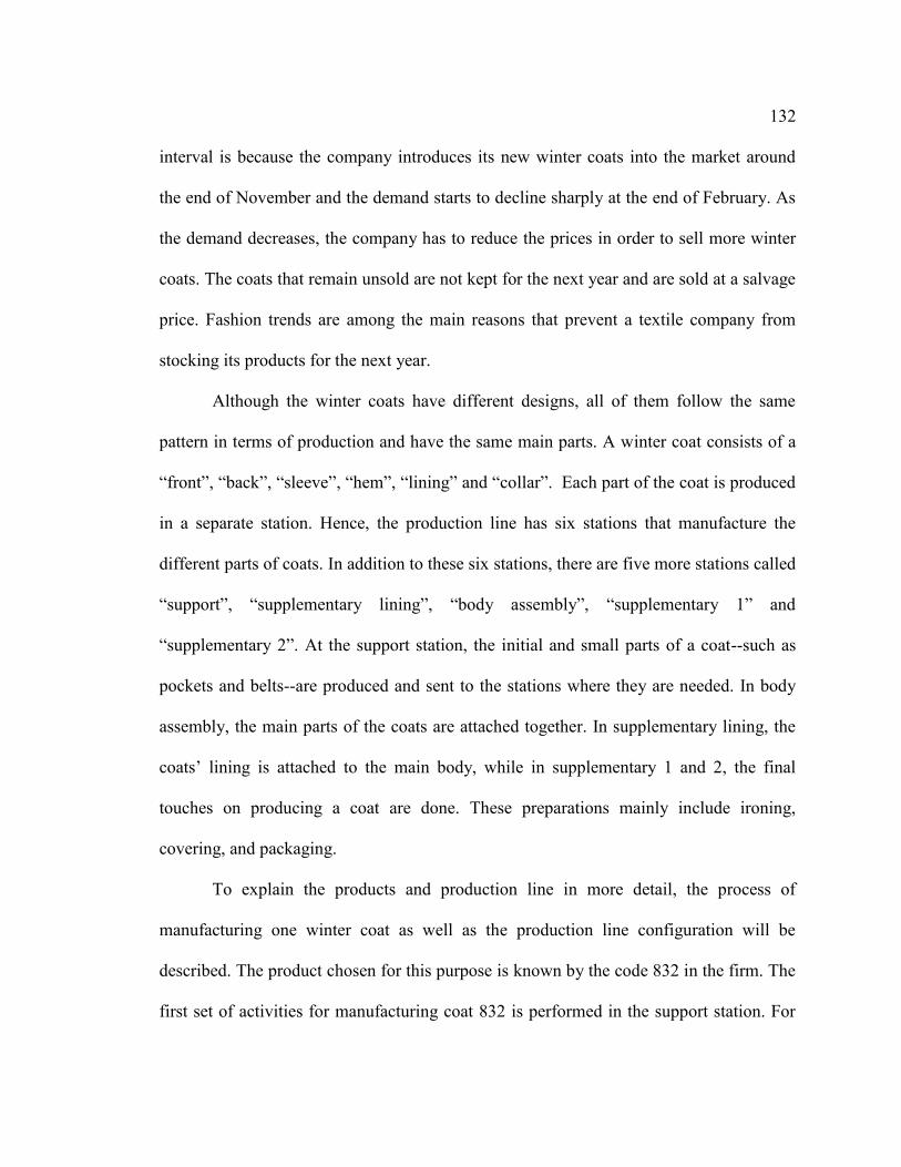
132 interval is because the company introduces its new winter coats into the market around

the end of November and the demand starts to decline sharply at the end of February. As

the demand decreases, the company has to reduce the prices in order to sell more winter

coats. The coats that remain unsold are not kept for the next year and are sold at a salvage

price. Fashion trends are among the main reasons that prevent a textile company from

stocking its products for the next year.

Although the winter coats have different designs, all of them follow the same

pattern in terms of production and have the same main parts. A winter coat consists of a

“front”, “back”, “sleeve”, “hem”, “lining” and “collar”. Each part of the coat is produced

in a separate station. Hence, the production line has six stations that manufacture the

different parts of coats. In addition to these six stations, there are five more stations called

“support”, “supplementary lining”, “body assembly”, “supplementary 1” and

“supplementary 2”. At the support station, the initial and small parts of a coat--such as

pockets and belts--are produced and sent to the stations where they are needed. In body

assembly, the main parts of the coats are attached together. In supplementary lining, the

coats’ lining is attached to the main body, while in supplementary 1 and 2, the final

touches on producing a coat are done. These preparations mainly include ironing,

covering, and packaging.

To explain the products and production line in more detail, the process of

manufacturing one winter coat as well as the production line configuration will be

described. The product chosen for this purpose is known by the code 832 in the firm. The

first set of activities for manufacturing coat 832 is performed in the support station. For

133 this purpose, different fabric parts, zippers, buttons, and pockets that are cut in the proper

sizes enter the support station. Figure 29 shows the material needed and the activities

involved in the support station for producing coat 832. Dark circles depict the input and

output of the support station in terms of material, while the round-cornered rectangular

shapes show the activities and their time in seconds.

Right upper hem

Right button piece

2

tagging

5

sewing

5

flapping

10

ironing

15

cutting

Right upper hem layer

15

sticking

27

aligning

Ready to use piece

Right hem

20

dressing

Figure 29. The material needed and activities involved in “support” station for producing coat 832

To perform the activities in the support station, a specific number of operators and

machines are needed. Figure 30 shows the standard configuration of the support station,

which is consists of three operators, four sewing machines, one iron table and four tables

for storing the works-in-progress (WIP).

134

20000.00

10000.00

1500

0.00

10000.00

15000.00 15000.00

10000.00

1500

0.00

5000.00 5000.00

1000

0.00

Sewing machine

Sew

ing machine

Sewing machine

Sw

ing machine

Ironing table

Figure 30. Support station standard configuration

In this configuration, two of the operators work with two sewing machines each

and the ironing table is controlled by one operator. The size of station’s equipment and

the space required is shown in the figure.

The output of the support station, in combination with the other material inputs

depicted in Figure 31, compose the inputs to the front station. The front of coat 832 has

two parts, namely the right and left front. These two parts are produced in the front

station.

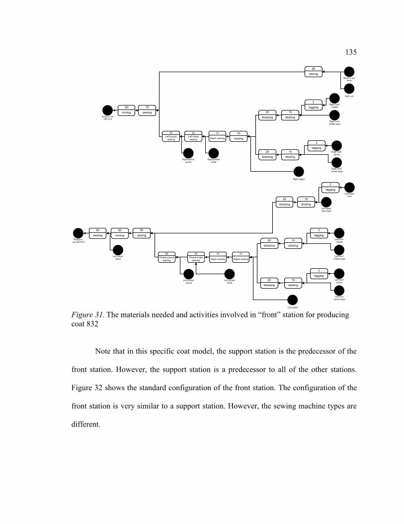
135

Right front middle

Right front middle layer

Right front corner

Right front corner layer

Right zipper

Left upper hem

Left front middle

Left front middle layer

Left front corner

Left front corner layer

Left zipper

Left button piece

2

tagging

2

tagging

15

sticking

15

sticking

70

sewing

Ready to use piece

Right hem

80

sewing

70

sewingReady to use

right front

2

tagging

Left upper hem layer

15

sticking

2

tagging

2

tagging

15

sticking

15

sticking

70

Seam sewing

50

sewing

80

sewingReady to

use left front

60

ironing

60

ironing

20

dressing

20

dressing

20

dressing

20

dressing

20

dressing

70

Seam sewing

70

Zipper sewing

Right pocket ticket

Right pocket pouch

20Left ticket

sewing

65Left pouch

sewing

Left pocket ticket

Left pocket pouch

20Pocket ticket

sewing

65Pocket pouch

sewing

Figure 31. The materials needed and activities involved in “front” station for producing coat 832

Note that in this specific coat model, the support station is the predecessor of the

front station. However, the support station is a predecessor to all of the other stations.

Figure 32 shows the standard configuration of the front station. The configuration of the

front station is very similar to a support station. However, the sewing machine types are

different.

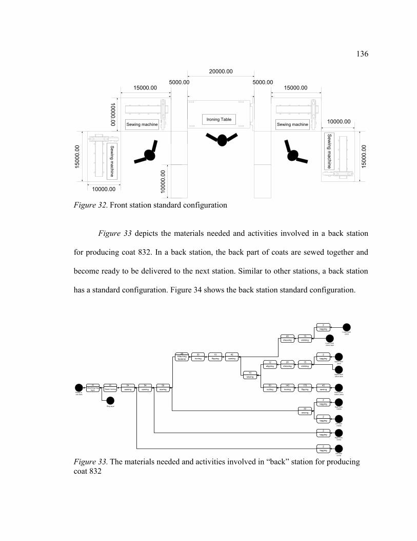
136

20000.00

10000.00

1500

0.00

10000.00

15000.00 15000.00

10000.00

1500

0.00

5000.00 5000.00

1000

0.00

Sewing machineSewing machine

Sew

ing machine

Sew

ing machine

Ironing Table

Figure 32. Front station standard configuration

Figure 33 depicts the materials needed and activities involved in a back station

for producing coat 832. In a back station, the back part of coats are sewed together and

become ready to be delivered to the next station. Similar to other stations, a back station

has a standard configuration. Figure 34 shows the back station standard configuration.

Lower back piece

Lower back piece layer

Upper back piece

Upper back piece layer

Back piece button piece

Right back middle

Left back middle

Right back corner

Left back corner

2

tagging

2

tagging

15

sticking

15

sticking

45

sewing

170

flipping

140

ironing

50

cutting

70

sewing

40

sewing

32

sewing

50

sewing

54

sewing

54

sewingReady to use back

60

Seam ironing

Ring layer

25Attaching ring

layer

2

tagging

2

tagging

2

tagging

2

tagging

20

dressing

20

dressing

12

aligning

10

flipping

30

ironing

20Attaching fastener

Figure 33. The materials needed and activities involved in “back” station for producing coat 832

137

15000.0020

000.

00 1000

0.00

10000.00

5000.00

10000.00

1500

0.00

Sewing machine

Sew

ing

mac

hine

Ironi

ng ta

ble

Figure 34. Back station standard configuration

Figure 35 shows the materials needed and activities involved at a sleeve station

for producing coat 832. The diagram has two separate parts for the right and left sleeves.

138

Right sleeve bigger piece

Right sleeve smaller piece

Right sleeve wrist

Right wrist button piece

Right wrist layer

Right wrist piece

20

sewing

15

sewing

5

flipping

10

ironing

10

cutting

15

alligning70

sewing

25

sewing

25

Seam ironing

30

sticking

25

sewing

20

Seam ironing

Ready to use right sleeve

Left sleeve bigger piece

Left sleeve smaller piece

Left sleeve wrist

Left wrist button piece

Left wrist layer

Left wrist piece

20

sewing

15sewing

5

flipping

10

ironing

10

cutting

15

alligning70

sewing

25

sewing

25

Seam ironing

30

sticking

25

sewing

20

Seam ironing

Ready to use left sleeve

2

tagging

2

tagging

2

tagging

2

tagging

2

tagging

2

tagging

Figure 35. The materials needed and activities involved in “sleeve” station for producing coat 832

The configuration of a sleeve station is similar to that of a back station. Figure 36

shows the sleeve station’s standard configuration.

15000.00

2000

0.00 10

000.

00

10000.00

5000.00

10000.00

1500

0.00

Sewing machine

Sew

ing machine

Ironi

ng ta

ble

Figure 36. Standard configuration of sleeve station

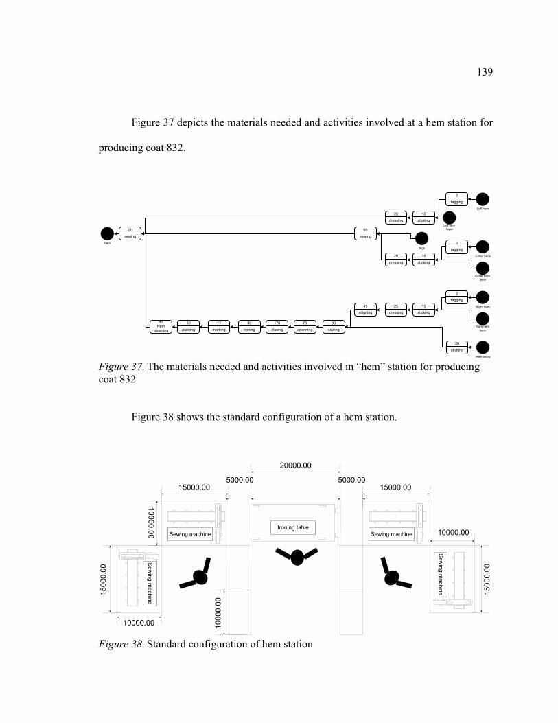
139

Figure 37 depicts the materials needed and activities involved at a hem station for

producing coat 832.

Left hem

Left hem layer

Collar back

Collar back layer

tags

Right hem

Right hem layer

Hem lining

2

tagging

15

sticking

25

dressing

2

tagging

15

sticking

20

dressing

60

sewing

2

tagging15

sticking

25

dressing

45

alligning

90

sewing

70

openning

170

closing

30

ironing

17

marking

30

piercing

20

sewing

hem

20

sticking

90Hem

fastening

Figure 37. The materials needed and activities involved in “hem” station for producing coat 832

Figure 38 shows the standard configuration of a hem station.

20000.00

10000.00

1500

0.00

10000.00

15000.00 15000.00

10000.00

1500

0.00

5000.00 5000.00

1000

0.00

Sewing machine

Sew

ing machine

Sew

ing machine

Sewing machineIroning table

Figure 38. Standard configuration of hem station

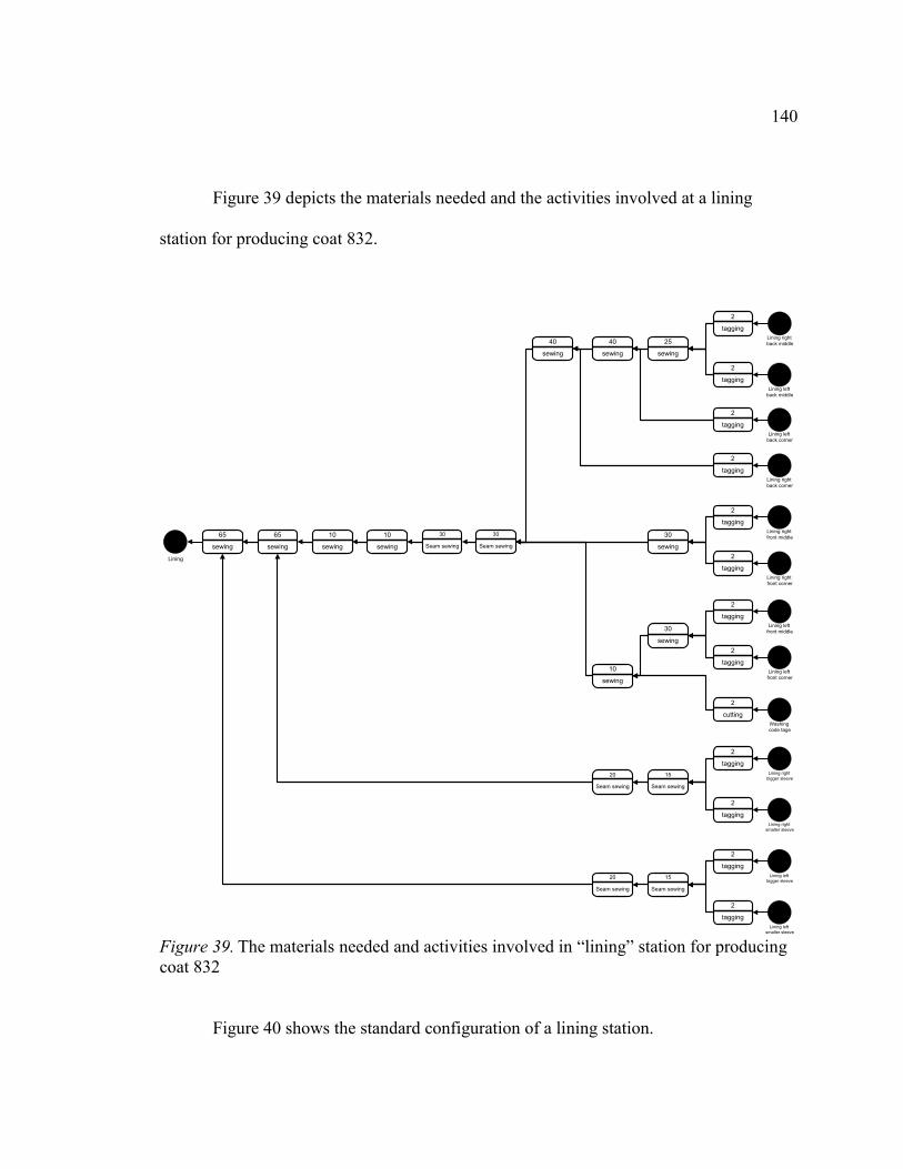
140

Figure 39 depicts the materials needed and the activities involved at a lining

station for producing coat 832.

Lining right back middle

Lining left back middle

Lining left back corner

Lining right back corner

Lining right front middle

Lining right front corner

Lining left front middle

Lining left front corner

Washing code tage

2

tagging

2

tagging

2

tagging

2

tagging

2

tagging

2

tagging

2

tagging

2

tagging

25

sewing

40

sewing

40

sewing

30

sewing

30

sewing

10

sewing

30

Seam sewing

30

Seam sewing

10

sewing

10

sewing

Lining right bigger sleeve

Lining right smaller sleeve

Lining left bigger sleeve

Lining left smaller sleeve

2

tagging

2

tagging

2

tagging

2

tagging

15

Seam sewing

20

Seam sewing

20

Seam sewing

15

Seam sewing

65

sewing

65

sewing

Lining

2

cutting

Figure 39. The materials needed and activities involved in “lining” station for producing coat 832

Figure 40 shows the standard configuration of a lining station.

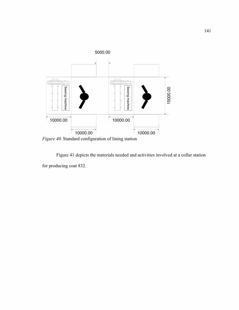
141

10000.00

10000.00

10000.00

10000.00

1500

0.00

5000.00

Sew

ing machine

Sew

ing machine

Figure 40. Standard configuration of lining station

Figure 41 depicts the materials needed and activities involved at a collar station

for producing coat 832.

142

Upper collar

Upper collar layer

Upper collar edge

Upper collar edge layer

2

tagging

15

sticking

2

tagging

15

sticking

20

dressing

20

dressing

35

sewing

60

ironing

Lower collar

Lower collar layer

Lower collar edge

Lower collar edge layer

2

tagging

15

sticking

2

tagging

15

sticking

20

dressing

20

dressing

35

sewing

20

aligning

30

aligning

30

aligning

20

aligning

collar

70

sewing

10

ironing

10

ironing

35

dressing

15

flipping

Figure 41. The materials needed and activities involved in “collar” station for producing coat 832

Figure 42 depicts the standard configuration of a collar station.

15000.00

2000

0.00 10

000.

00

10000.00

5000.00

10000.00

1500

0.00

Sewing machine

Sew

ing machine

Ironi

ng ta

ble

Figure 42. Standard configuration of collar station

143

Figure 43 shows the materials needed and activities involved at a body assembly

station for producing coat 832. At a body assembly station the main parts of the coat are

sewed together.

layer

Ready to use right front

Ready to use left front

Ready to use back

50

Seam sewing

50

Seam sewing

10

sewing

10

sewing

70

ironing

40

sticking

Right sleeveLeft sleeve

40

sewing

65

sewing

65

sewing

foamfoam

80

sewing

70

sewing

Body

Figure 43. The materials needed and activities involved in “body assembly” station for producing coat 832

Figure 44 depicts the standard configuration of a body assembly station.

20000.00

10000.00

1500

0.00

10000.00

15000.00 15000.00

10000.00

1500

0.00

5000.00 5000.00

1000

0.00

Sewing machine Sewing machine

Sew

ing machine

Sew

ing machine

Ironing table

Figure 44. Standard configuration of body assembly station

Figure 45 shows the materials needed and activities involved at a supplementary

lining station for producing coat 832.

144

Hem

Lining

185

sewing

60

aewing

140

ironingComplete

Lining

Figure 45. The materials needed and activities involved in “supplementary lining” station for producing coat 832

Figure 46 depicts the standard configuration of a supplementary lining station.

15000.00

2000

0.00 10

000.

00

10000.00

5000.00

10000.00

1500

0.00

Sewing machine

Sew

ing machine

Ironi

ng ta

ble

Figure 46. Standard configuration of supplementary lining station

Figure 47 shows the materials needed and activities involved at “supplementary

1” station for producing coat 832.

145

Body

Complete lining

45

aligning

170

sewing

180

dressing

120

Seam sewing

60

sewing

45

sewing

45

sewing

65

sewing

130

flipping

250

ironing

Collar

260

sewing

30

sewing

30

tucking

90

ironing

130

sewing

35

sewing

150

Button sewingSemi

finished good

Figure 47. The materials needed and activities involved in “supplementary 1” station for producing coat 832

Figure 48 shows the standard configuration of a supplementary 1 station. Note

that at a supplementary 1 station that is performing ironing activities, two operators are

needed.

20000.00

1000

0.00

15000.00

10000.0015

000.

00

10000.00

15000.00

1000

0.00

15000.00

1500

0.00

Sewing machine

Sewing machine

Sewing machineSewing machine

Sew

ing

mac

hine

Sew

ing

mac

hine

Ironing table

Figure 48. Standard configuration of a supplementary 1 station

Figure 49 shows the materials needed and activities involved at a “supplementary

2” station for producing coat 832. Note that one of the activities depicted in Figure 49 is

shown in a diamond form, which is a control activity. Although the quality of the

products is monitored throughout the entire production line, since this specific control

activity is performed by the operators of the shop floor, it is included in the diagram.

146

25

alining

15

piercing

200

sewingControl

240

60

ironing

480

ironing

30

buttoning

15

Tag hanging

55

Covering

360

BlowingSemi finished

goodCoat 832 Figure 49. The materials needed and activities involved in “supplementary 2” station for producing coat 832

Figure 50 depicts the standard configuration of a supplementary 2 station.

20000.00 15000.00

1500

0.00

20000.00

10000.00

Sewing machine

Mannequin iron

Covering table Covering table

Ironing table

Figure 50. Standard configuration of supplementary 2 station

The shop floor stations are designed flexibly and can adapt to new product

requirements. In addition, it is possible to adjust the production capacity by adding or

reducing the number of operators at each station. However, due to human resource

constraints, only 32 operators can be assigned to the production line. Figure 51 shows the

overall shop floor layout and arrangement of stations.

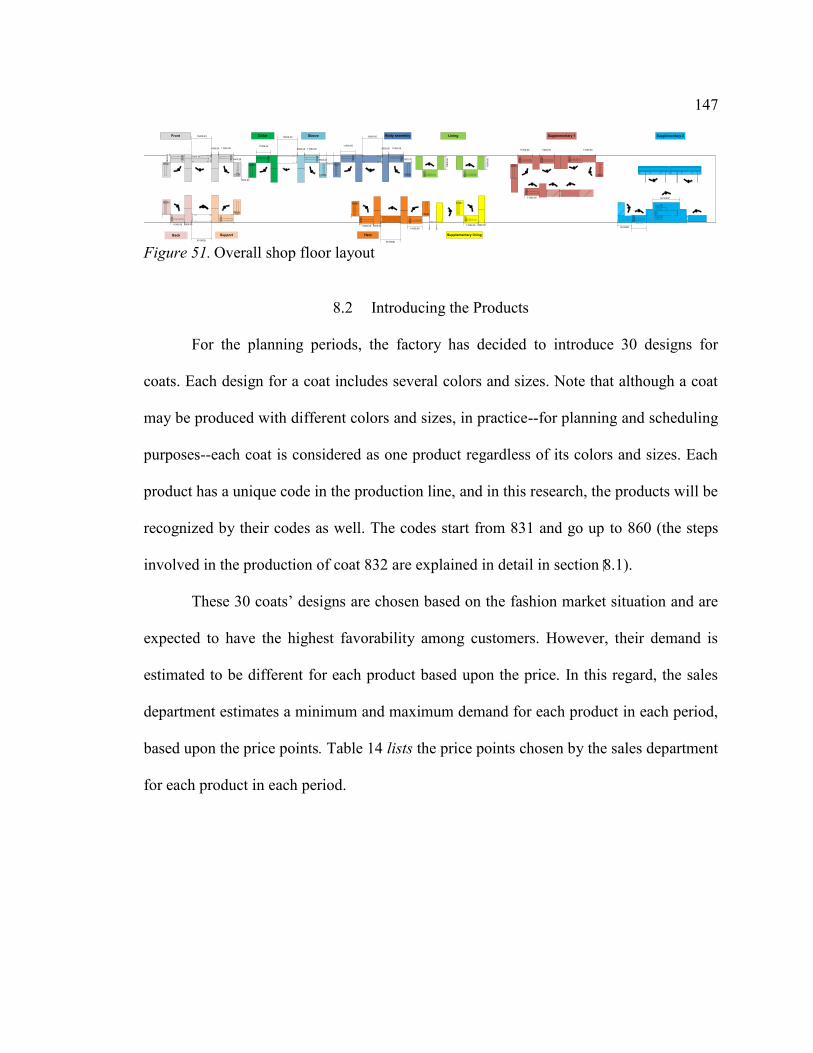
147

15000.00

5503.20

5000.00

20000.08

5000.00

5000.00

1000

0.00

5000.00

20000.00

10000.00

11000.00

5503

.20

5503.20

5000.0011000.00

5503

.20

15000.00

5503.20

5000.00 11000.00

15000.00

11000.00

5503.20

5000.00 11000.00

15000.00

11000.00

5000.00

5503.20

5000.0011000.00

15000.00

11000.00

1000

0.00

5000.0011000.00

11000.00

11000.00 11000.00 11000.00

11000.00

Front

Back Support

SleeveCollar

Hem

LiningBody assembly

Supplementary lining

Supplementary 2Supplementary 1

Figure 51. Overall shop floor layout

8.2 Introducing the Products

For the planning periods, the factory has decided to introduce 30 designs for

coats. Each design for a coat includes several colors and sizes. Note that although a coat

may be produced with different colors and sizes, in practice--for planning and scheduling

purposes--each coat is considered as one product regardless of its colors and sizes. Each

product has a unique code in the production line, and in this research, the products will be

recognized by their codes as well. The codes start from 831 and go up to 860 (the steps

involved in the production of coat 832 are explained in detail in section ‎8.1).

These 30 coats’ designs are chosen based on the fashion market situation and are

expected to have the highest favorability among customers. However, their demand is

estimated to be different for each product based upon the price. In this regard, the sales

department estimates a minimum and maximum demand for each product in each period,

based upon the price points. Table 14 lists the price points chosen by the sales department

for each product in each period.

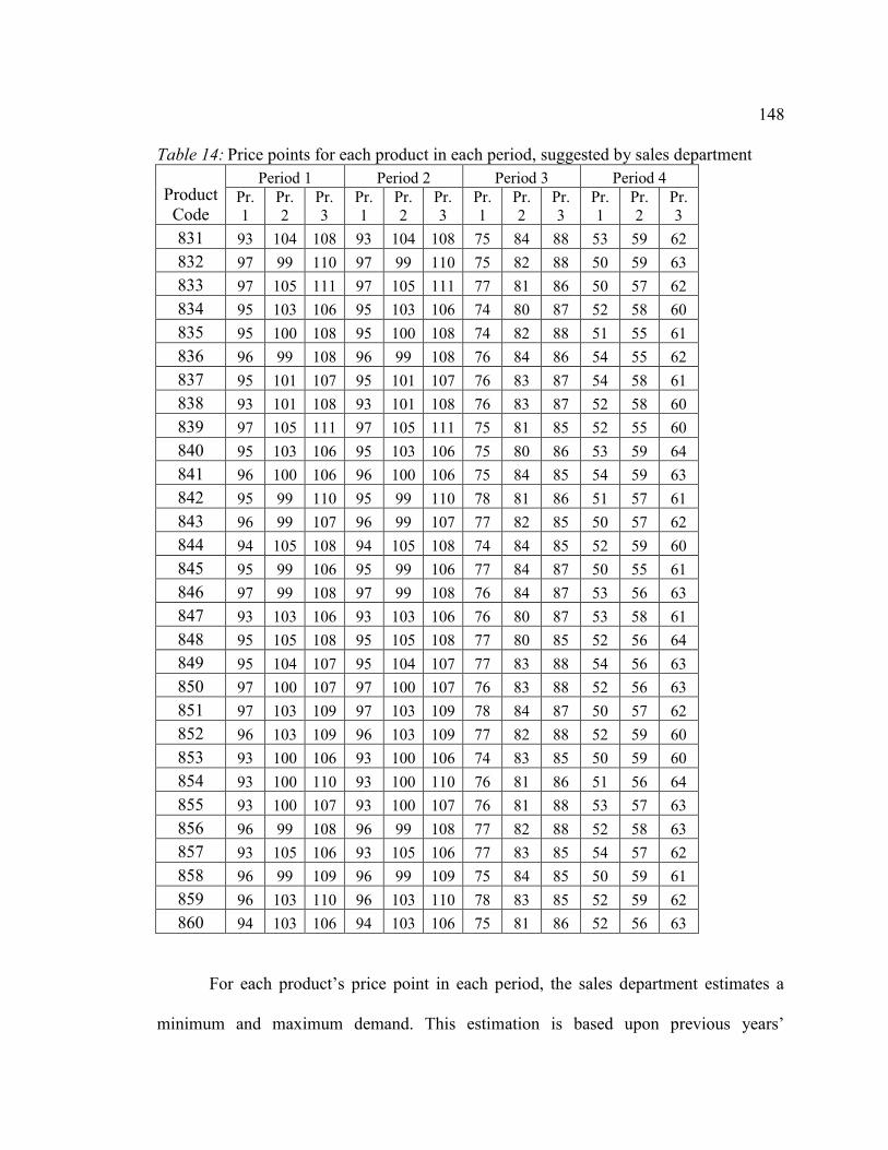
148 Table 14: Price points for each product in each period, suggested by sales department

Product Code

Period 1 Period 2 Period 3 Period 4 Pr. 1

Pr. 2

Pr. 3

Pr. 1

Pr. 2

Pr. 3

Pr. 1

Pr. 2

Pr. 3

Pr. 1

Pr. 2

Pr. 3

831 93 104 108 93 104 108 75 84 88 53 59 62 832 97 99 110 97 99 110 75 82 88 50 59 63 833 97 105 111 97 105 111 77 81 86 50 57 62 834 95 103 106 95 103 106 74 80 87 52 58 60 835 95 100 108 95 100 108 74 82 88 51 55 61 836 96 99 108 96 99 108 76 84 86 54 55 62 837 95 101 107 95 101 107 76 83 87 54 58 61 838 93 101 108 93 101 108 76 83 87 52 58 60 839 97 105 111 97 105 111 75 81 85 52 55 60 840 95 103 106 95 103 106 75 80 86 53 59 64 841 96 100 106 96 100 106 75 84 85 54 59 63 842 95 99 110 95 99 110 78 81 86 51 57 61 843 96 99 107 96 99 107 77 82 85 50 57 62 844 94 105 108 94 105 108 74 84 85 52 59 60 845 95 99 106 95 99 106 77 84 87 50 55 61 846 97 99 108 97 99 108 76 84 87 53 56 63 847 93 103 106 93 103 106 76 80 87 53 58 61 848 95 105 108 95 105 108 77 80 85 52 56 64 849 95 104 107 95 104 107 77 83 88 54 56 63 850 97 100 107 97 100 107 76 83 88 52 56 63 851 97 103 109 97 103 109 78 84 87 50 57 62 852 96 103 109 96 103 109 77 82 88 52 59 60 853 93 100 106 93 100 106 74 83 85 50 59 60 854 93 100 110 93 100 110 76 81 86 51 56 64 855 93 100 107 93 100 107 76 81 88 53 57 63 856 96 99 108 96 99 108 77 82 88 52 58 63 857 93 105 106 93 105 106 77 83 85 54 57 62 858 96 99 109 96 99 109 75 84 85 50 59 61 859 96 103 110 96 103 110 78 83 85 52 59 62 860 94 103 106 94 103 106 75 81 86 52 56 63

For each product’s price point in each period, the sales department estimates a

minimum and maximum demand. This estimation is based upon previous years’

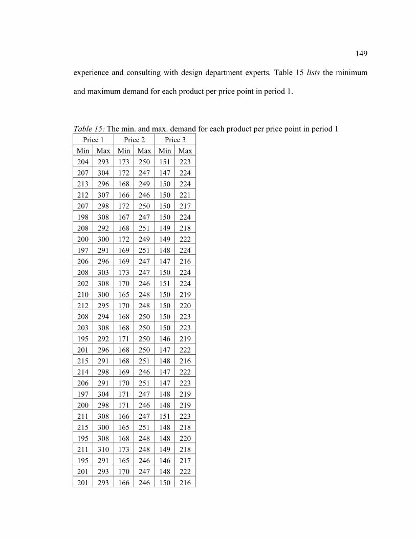
149 experience and consulting with design department experts. Table 15 lists the minimum

and maximum demand for each product per price point in period 1.

Table 15: The min. and max. demand for each product per price point in period 1

Price 1 Price 2 Price 3 Min Max Min Max Min Max 204 293 173 250 151 223 207 304 172 247 147 224 213 296 168 249 150 224 212 307 166 246 150 221 207 298 172 250 150 217 198 308 167 247 150 224 208 292 168 251 149 218 200 300 172 249 149 222 197 291 169 251 148 224 206 296 169 247 147 216 208 303 173 247 150 224 202 308 170 246 151 224 210 300 165 248 150 219 212 295 170 248 150 220 208 294 168 250 150 223 203 308 168 250 150 223 195 292 171 250 146 219 201 296 168 250 147 222 215 291 168 251 148 216 214 298 169 246 147 222 206 291 170 251 147 223 197 304 171 247 148 219 200 298 171 246 148 219 211 308 166 247 151 223 215 300 165 251 148 218 195 308 168 248 148 220 211 310 173 248 149 218 195 291 165 246 146 217 201 293 170 247 148 222 201 293 166 246 150 216

150

Table 16 lists the minimum and maximum demand for each product per price point

in period 2.



151

Table 17 lists the minimum and maximum demand for each product per price

point in period 3.



152

Table 18 lists the minimum and maximum demand for each product per price

point in period 4.


Price 1 Price 2 Price 3 Min Max Min Max Min Max 101 176 80 137 46 77 99 169 83 126 52 71

100 174 82 130 46 71 103 169 79 132 54 81 104 172 83 127 53 76 97 173 75 124 49 75

100 175 81 133 50 71 97 175 85 134 51 74

100 175 78 125 45 76 101 174 75 126 45 74 96 170 76 128 44 78

102 169 85 126 45 71 103 173 81 124 48 82 95 172 78 131 54 79 99 175 81 125 49 72

103 167 84 127 46 72 104 166 85 129 49 75 96 168 84 136 47 74

104 171 78 137 45 81 97 176 78 133 45 78 98 170 79 136 52 77 96 176 77 134 47 71

102 169 82 127 48 76 103 167 75 137 45 71 96 168 80 137 46 81

101 167 81 132 51 71 104 167 81 133 50 77 100 168 75 132 48 79 100 166 83 135 45 71 104 170 75 134 45 80

153

8.3 Estimating the Costs and Resource Constraints

Using the method described for cost estimation in section ‎4, production,

inventory, and lost sale costs are then estimated. Table 19 lists the estimated costs.

Note that, due to the geometrical similarity of the coats, their inventory cost is

estimated to be the same ($2 per item per period). Considering the same logic, each coat

occupies one single space in the warehouse and hence, the space consumption coefficient

for all of the coats is 1.

The coat's factory warehouse has enough capacity for stocking 5000 coats.

Considering that each station in the production line is designed to deliver output in a

maximum of 5 minutes and there are 10 working hours per day, the production capacity

is 120 items per day. Hence, with 25 working days in a month, the monthly production

capacity is products. The management can assign budget for

production of a total 15000 coats, considering the average production costs. Hence, the

budget constraint is not expected to be active in the planning model.

154 Table 19: Estimated production, inventory, and lost sale costs for products

Product Code

Production Cost

Inventory Cost

Lost Sale Cost

831 43 2 11 832 43 2 11 833 49 2 9 834 49 2 9 835 48 2 9 836 41 2 11 837 47 2 10 838 41 2 11 839 46 2 10 840 50 2 9 841 50 2 9 842 43 2 11 843 40 2 11 844 44 2 10 845 41 2 11 846 41 2 11 847 48 2 9 848 40 2 11 849 46 2 10 850 41 2 11 851 44 2 10 852 44 2 10 853 44 2 10 854 43 2 11 855 49 2 9 856 45 2 10 857 40 2 11 858 42 2 11 859 49 2 9 860 41 2 11

155

8.4 Pricing, Planning and Price of Robustness

Based on the data introduced in sections ‎8.2 and ‎8.3, the first step in

implementing the decision support system is to calculate the prices and then plan for the

horizon. Using the mathematical model and technique introduced in section ‎5, the

problem is solved using CPLEX software that yields the exact solution and the proposed

unconscious search where the uncertainty budget parameter is zero, i.e. . Note that

when , all the demands are considered to be exact, and hence no uncertainty is

considered in the problem.

CPLEX takes more than 11 minutes and terminates the solving procedure due to

an out-of-memory error. However, unconscious search (US) finds a good solution in less

than 10 seconds. Note that the memory of the computer used for this research is 12.0 GB,

and the processor has a core i7 3.40 GHz.

The value of the objective function obtained by US, which is the maximized profit

by a pricing and planning agent, is equal to $482,978. Table 20 lists the prices obtained

by the pricing and planning module for each period. For the first three periods, all the

prices are chosen to be at the highest possible. However, as the demand decreases in the

last period, most of the prices chosen are less than the highest possible. This trend tends

to go well with intuition.

Table 21 list the production plan for each product in each period. Some products

are planned to be produced in specific periods. However, this trend does not apply to the

last period, where all the products are placed in the production plan. The reason may be

156 that, as the demand falls, the profit margin of all the products gets closer to each other,

and hence, it is profitable to produce all products.

Table 20: Prices obtained by pricing and planning module for each period ($)

Product Period

1 Period

2 Period

3 Period

4 831 108 108 88 59 832 110 110 88 59 833 111 111 86 62 834 106 106 87 58 835 108 108 88 61 836 108 108 86 54 837 107 107 87 58 838 108 108 87 58 839 111 111 85 60 840 106 106 86 64 841 106 106 85 59 842 110 110 86 57 843 107 107 85 57 844 108 108 85 59 845 106 106 87 55 846 108 108 87 56 847 106 106 87 58 848 108 108 85 56 849 107 107 88 63 850 107 107 88 56 851 109 109 87 57 852 109 109 88 59 853 106 106 85 59 854 110 110 86 56 855 107 107 88 63 856 108 108 88 58 857 106 106 85 54 858 109 109 85 59 859 110 110 85 59 860 106 106 86 56

157

Table 21: Production plan obtained by pricing and planning module

Product Period 1

Period 2

Period 3

Period 4

831 187 153 200 109 832 186 237 200 105 833 0 0 0 59 834 0 0 0 106 835 0 0 0 65 836 187 237 201 135 837 0 0 0 107 838 186 230 202 110 839 32 0 0 61 840 0 0 0 60 841 0 0 0 102 842 188 239 198 106 843 185 235 196 103 844 0 0 0 105 845 187 234 202 103 846 187 236 197 106 847 0 0 0 107 848 185 238 196 110 849 0 0 0 63 850 185 242 202 106 851 185 0 5 108 852 184 0 199 106 853 0 0 0 105 854 187 238 205 106 855 0 0 0 64 856 0 0 0 107 857 184 240 200 136 858 182 241 198 104 859 0 0 0 109 860 183 0 199 105

158

Due to inventory costs, the plan obtained by the pricing and planning module is

arranged in a way to keep zero inventory at the end of the month. Thus, the sales plan is

expected to be similar to the production plan.

One interesting aspect of the pricing and planning module’s output is the ability to

calculate the increased profit due to the increased capacity. In other words, it is possible

to ask how much the profit could be increased by increasing the production capacity.

Answering this question can help management to understand and calculate the most

profitable amount of investment in production utilities and machines.

To obtain the relationship between capacity and profit, the pricing and planning

module has calculated the profit taking into account the different production capacities.

Figure 52 depicts the relationship between production capacity and profit. As is expected,

by increasing the production capacity, the profit increases. However, the amount by

which the profit is increased has a decaying slope until it reaches the zero point, when

production capacity is approximately 11000.

Figure 52. Increase in profit as the production capacity increases

0200000400000600000800000

100000012000001400000

0 2000 4000 6000 8000 10000 12000 14000

Prof

it

Production Capacity (per period)

159

To consider the demands associated with prices in an uncertain setting, the

uncertainty budget parameter needs to be greater than zero, i.e. . In this case,

although the uncertain demand has been taken into consideration, the optimum solution

will be decreased. The difference between the exact problem optimum value and the

uncertain problem optimum solution is the price of robustness. From a managerial point

of view, the price of robustness is the cost that the system accepts in order to handle the

uncertainty robustly.

To evaluate the price of robustness, the best value of the objective function is

calculated per the different values of . Figure 53 shows the price of robustness as the

uncertainty budget parameter increases. As expected, the graph increases monotonically

as the uncertainty budget parameter increases. According to Figure 53, if a worst-case

scenario is considered for this problem, $4339 will be imposed on the best-found value of

the objective function, which is less than 1% of the deterministic objective function

value. As the increases, the probability of a constraint to be violated due to

uncertainty decreases. This probability becomes zero when .

160

Figure 53. Price of robustness per different values of uncertainty budget parameter

To proceed to the scheduling module of the proposed decision support system, it

is necessary to choose a plan with a specific level of robustness. The management of the

textile firm believes that considering the worst-case scenario does not impose too much

expense, and since it has considered the uncertainty fully, the worst-case scenario is

chosen for the production plan. Table 22 tabulates the production plan for the worst-case

scenario for each period.

0

500

1000

1500

2000

2500

3000

3500

4000

4500

5000

0 20 40 60 80 100 120 140

Pric

e of

Rob

ustn

ess

Uncertainty Budget Parameter

161 Table 22: Production plan for worst-case scenario

Product Period 1

Period 2

Period 3

Period 4

831 187 0 200 109 832 186 237 200 105 833 0 0 0 59 834 0 0 0 106 835 0 0 0 65 836 187 237 201 135 837 0 0 0 107 838 186 230 202 110 839 186 0 0 61 840 0 0 0 60 841 0 0 0 102 842 188 239 198 106 843 185 235 196 103 844 0 0 0 105 845 187 234 202 103 846 187 236 197 106 847 0 0 0 107 848 185 238 196 110 849 0 0 0 63 850 185 242 202 106 851 185 0 5 108 852 30 0 199 106 853 0 0 0 105 854 187 238 205 106 855 0 0 0 64 856 0 0 0 107 857 184 240 200 136 858 182 241 198 104 859 0 0 0 109 860 183 153 199 105

Table 23 tabulates the chosen prices for each product in each period for the worst-

case scenario.

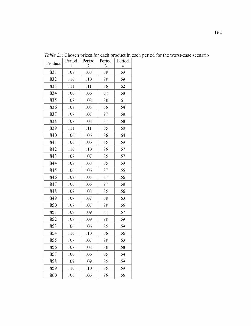
162

Table 23: Chosen prices for each product in each period for the worst-case scenario

Product Period 1

Period 2

Period 3

Period 4

831 108 108 88 59 832 110 110 88 59 833 111 111 86 62 834 106 106 87 58 835 108 108 88 61 836 108 108 86 54 837 107 107 87 58 838 108 108 87 58 839 111 111 85 60 840 106 106 86 64 841 106 106 85 59 842 110 110 86 57 843 107 107 85 57 844 108 108 85 59 845 106 106 87 55 846 108 108 87 56 847 106 106 87 58 848 108 108 85 56 849 107 107 88 63 850 107 107 88 56 851 109 109 87 57 852 109 109 88 59 853 106 106 85 59 854 110 110 86 56 855 107 107 88 63 856 108 108 88 58 857 106 106 85 54 858 109 109 85 59 859 110 110 85 59 860 106 106 86 56

163

8.5 Scheduling

Using the output of the pricing and planning module and other necessary inputs

described in section ‎6, the scheduling module can optimize the job sequence. The

products and their production plan obtained in the pricing and planning module are

considered jobs. The beginning and finish time of each time period is considered the

release time and due date of the jobs. Hence, if 187 units of coat 831 are to be produced

in the first period, the beginning and finish time of the first period are considered as the

release time and due date of producing these 187 units.

The working hours of the shop floor are from 9:00 to 19:00, and the maintenance

times are scheduled during non-working hours. Thus, the only valid interval for

scheduling the tasks is from 9:00 to 19:00. Note that having a working timeline with

some time intervals that are not allowed to be scheduled, as well as jobs with various

release times, can dramatically add to the complexity of the scheduling problem.

For each product, it is necessary to define the operation chart and have its cycle

times on each shop floor station. In the proposed decision support system, this is possible

by a graphical user interface that gives the user the ability of defining operations charts

by drawing the process flow. Figure 54 shows the user interface for defining the

operations chart for coat 832. As can be observed in Figure 54, it is possible to define the

operations chart of the product in a network format. In each station, the list of necessary

activities with their cycle times, required human resources, materials, and machines are

stored. Hence, it is possible to calculate processing times and the necessary resources for

job scheduling. All of the cycle times are between 200 to 300 seconds for each product

164 and station. In addition, due to labor-intensive nature of the production processes, each

processing time has to be given some leeway, with 20 seconds as the maximum possible

deviation from the average. Thus, the processing time for each product in each station has

a triangular distribution.

Setup times for each product can be defined dependently. However, in this case

the setup times are independent and very small. Thus, it is possible to ignore them. Note

that, the method used in the scheduling module can handle dependent setup times as well.

Figure 54. User interface for defining operation process of coat 832

165

In addition to the inputs for optimizing the schedule, it is necessary to define the

objective function of the scheduling module as well. Three objective functions are

considered in this case; make span, total finish time, and total tardiness. Figure 55 shows

the user interface of the decision support system in which the jobs, their due dates,

release times, weights, and objective function can be defined.

Figure 55. User interface for defining the jobs and choosing the objective function

For the case chosen, the objective function preferred by the management is make

span. Note that tardiness is not chosen due to the low lost sale costs for each product.

However, in a different industry such as automotive, it seems logical to use total tardiness

as an objective function due to the high lost sale costs associated with products and the

high costs of stopping the manufacturer production line by the supplier due to late

production.

Considering the make span as the objective function, the scheduling module

optimizes the sequence of the jobs in order to minimize the make span. In total, 77

products with all their respective production stations, activities, and necessary resources,

166 need to be scheduled in a four-month period. After running the scheduling algorithm, it

takes approximately 20 seconds to come up with a schedule. Note that the user can

accept, reject, or modify the schedule. Figure 56 shows the schedule for three days – i.e.

November 8th, 9th, and 10th. Each color shows a product.

After scheduling the products, no delay was observed in the jobs, and the total

tardiness was zero. In each time period, approximately 20% of the time is not scheduled,

which is due to the possible variations in processing times and unscheduled stoppages.

This is completely in accordance with the historical performance of the factory. This

shows that the scheduling module has successfully considered the probabilistic nature of

the tasks.

Figure 56. User interface for scheduling November 8th, 9th., and 10th

8.6 Inventory Management

In each winter coat, three types of fabric are used for the outer layer, the lining,

and the middle layer. Since the outer layer and the lining are visible, their color needs to

be matched. However, the middle layer is invisible and can be any color. In total, 21

167 different fabrics are chosen for the designed winter coats, among which 10 are for the

outer layer, 10 are for the lining, and one is for the middle layer. Table 24 lists the fabric

consumption for each product. (The unit of consumption chosen is the yard.) Note that,

although there are other materials such as buttons and threads necessary for producing a

coat, since their prices are very low compared to the fabrics, they are not included in the

inventory management module.

There are five suppliers that provide the fabrics to the factory. However, since

these suppliers are located in different regions, the ordering costs are different. Note that

for each order, it is necessary that a team from the design department go to the supplier

site and introduce the necessary quality specifications. Hence, the main cost associated

with ordering a fabric is the cost of relocating the design team. The ordering cost of the

first and second suppliers is approximately $500, while for the rest of the suppliers, this

cost is approximately $300.

168 Table 24: Fabric consumption for each product (yard)

Product Outer Layer Lining Middle

Layer 830 3.1 2.4 1.8 831 2.9 2.2 1.6 832 2.8 2.1 1.5 833 3.2 2.5 1.9 834 2.5 1.8 1.2 835 2.8 2.1 1.5 836 2.9 2.2 1.6 837 2.6 1.9 1.3 838 2.6 1.9 1.3 839 2.9 2.2 1.6 840 2.9 2.2 1.6 841 2.8 2.1 1.5 842 2.9 2.2 1.6 843 2.8 2.1 1.5 844 3 2.3 1.7 845 2.9 2.2 1.6 846 3.1 2.4 1.8 847 2.5 1.8 1.2 848 2.6 1.9 1.3 849 2.9 2.2 1.6 850 2.7 2 1.4 851 2.7 2 1.4 852 3.1 2.4 1.8 853 3.1 2.4 1.8 854 3.1 2.4 1.8 855 2.9 2.2 1.6 856 2.5 1.8 1.2 857 2.6 1.9 1.3 858 3.1 2.4 1.8 859 2.5 1.8 1.2

169

The inventory cost of all the fabrics is approximately $0.4. All of the suppliers

offer nearly the same purchasing price. However, there are small variations. Table 25 lists

the purchasing cost of a unit of each fabric from each supplier.

Table 25: Purchasing cost of each fabric from different suppliers

Fabric Supplier 1

Supplier 2

Supplier 3

Supplier 4

Supplier 5

1 2 2 2.1 2 2 2 1.8 2.1 2.1 1.8 2 3 1.9 2.1 2 1.9 1.9 4 1.8 2.1 2.1 1.8 2 5 1.8 2.1 2.2 1.8 2 6 2 2.1 2.1 2 2.1 7 1.9 2.1 2 1.8 2 8 2 2.1 2 1.8 2 9 1.8 2 2 2 2.1 10 1.9 2.1 2.1 2 2 11 1.9 1.9 2.2 1.9 2 12 1.8 1.9 2 1.9 2 13 1.9 1.9 2.1 1.8 2 14 1.9 2.1 2 1.9 2 15 1.8 1.9 2.1 1.9 1.9 16 1.9 2 2.1 1.9 2 17 1.9 2 2.2 1.9 1.9 18 1.9 1.9 2.2 2 2 19 1.8 2.1 2.1 1.8 2 20 2 2 2.2 2 2 21 2 1.9 2.1 1.9 2.1

In addition to the costs, it is necessary to determine the demand for each fabric.

Using the fabric consumption listed in Table 24 and the production plan in each period, it

is possible to take the output of the production plan and schedule it into the material plan.

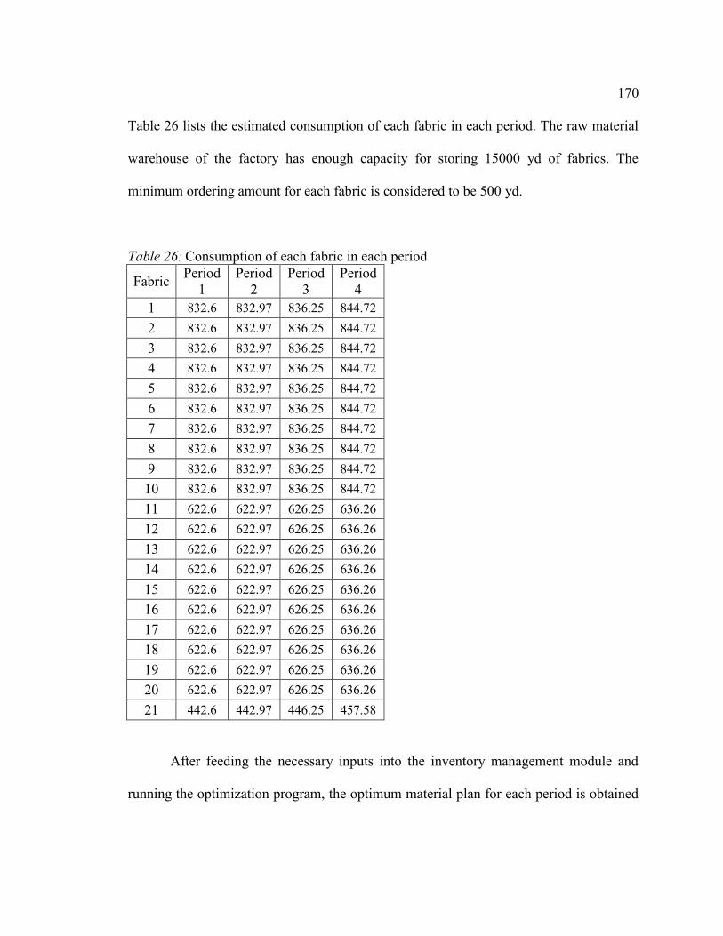
170 Table 26 lists the estimated consumption of each fabric in each period. The raw material

warehouse of the factory has enough capacity for storing 15000 yd of fabrics. The

minimum ordering amount for each fabric is considered to be 500 yd.

Table 26: Consumption of each fabric in each period

Fabric Period 1

Period 2

Period 3

Period 4

1 832.6 832.97 836.25 844.72 2 832.6 832.97 836.25 844.72 3 832.6 832.97 836.25 844.72 4 832.6 832.97 836.25 844.72 5 832.6 832.97 836.25 844.72 6 832.6 832.97 836.25 844.72 7 832.6 832.97 836.25 844.72 8 832.6 832.97 836.25 844.72 9 832.6 832.97 836.25 844.72 10 832.6 832.97 836.25 844.72 11 622.6 622.97 626.25 636.26 12 622.6 622.97 626.25 636.26 13 622.6 622.97 626.25 636.26 14 622.6 622.97 626.25 636.26 15 622.6 622.97 626.25 636.26 16 622.6 622.97 626.25 636.26 17 622.6 622.97 626.25 636.26 18 622.6 622.97 626.25 636.26 19 622.6 622.97 626.25 636.26 20 622.6 622.97 626.25 636.26 21 442.6 442.97 446.25 457.58

After feeding the necessary inputs into the inventory management module and

running the optimization program, the optimum material plan for each period is obtained

171 with an objective function value of $138101.9. Table 27 shows the material plan for each

fabric that needs to be ordered by a specific supplier in periods 1 and 2.

Table 27: Material plan for each fabric that needs to be ordered by a specific supplier in periods 1 and 2

Fabric Period 1 Period 2

S1 S2 S3 S4 S5 S1 S2 S3 S4 S5 1 0 0 0 832.6 0 0 0 0 0 832.97 2 0 0 0 832.6 0 0 0 0 832.97 0 3 0 0 0 0 832.6 0 0 0 0 832.97 4 0 0 0 832.6 0 0 0 0 832.97 0 5 0 0 0 832.6 0 0 0 0 832.97 0 6 0 0 0 832.6 0 0 0 0 832.97 0 7 0 0 0 832.6 0 0 0 0 832.97 0 8 0 0 0 832.6 0 0 0 0 832.97 0 9 1665.6 0 0 0 0 0 0 0 0 0

10 0 0 0 832.6 0 0 0 0 832.97 0 11 0 0 0 1245.6 0 0 0 0 0 0 12 0 0 0 1245.6 0 0 0 0 0 0 13 0 0 0 1245.6 0 0 0 0 0 0 14 0 0 0 1245.6 0 0 0 0 0 0 15 0 0 0 1245.6 0 0 0 0 0 0 16 0 0 0 1245.6 0 0 0 0 0 0 17 0 0 0 0 1245.6 0 0 0 0 0 18 0 0 0 1245.6 0 0 0 0 0 0 19 0 0 0 1245.6 0 0 0 0 0 0 20 0 0 0 0 1245.6 0 0 0 0 0 21 0 0 0 885.57 0 0 0 0 0 0

Table 28 shows the material plan for each fabric that needs to be ordered by a

specific supplier in periods 3 and 4.

172 Table 28: Material plan for each fabric that needs to be ordered by a specific supplier in periods 3 and 4

Fabric Period 3 Period 4

S1 S2 S3 S4 S5 S1 S2 S3 S4 S5 1 0 0 0 0 836.25 0 0 0 0 844.72 2 0 0 0 836.25 0 0 0 0 844.72 0 3 0 0 0 0 836.25 0 0 0 0 844.72 4 0 0 0 836.25 0 0 0 0 844.72 0 5 0 0 0 836.25 0 0 0 0 844.72 0 6 0 0 0 836.25 0 0 0 0 844.72 0 7 0 0 0 836.25 0 0 0 0 844.72 0 8 0 0 0 836.25 0 0 0 0 844.72 0 9 1680.97 0 0 0 0 0 0 0 0 0

10 0 0 0 836.25 0 0 0 0 0 844.72 11 0 0 0 1262.51 0 0 0 0 0 0 12 0 0 0 1262.51 0 0 0 0 0 0 13 0 0 0 1262.51 0 0 0 0 0 0 14 0 0 0 1262.51 0 0 0 0 0 0 15 0 0 0 1262.51 0 0 0 0 0 0 16 0 0 0 1262.51 0 0 0 0 0 0 17 0 0 0 0 1262.51 0 0 0 0 0 18 0 0 0 1262.51 0 0 0 0 0 0 19 0 0 0 1262.51 0 0 0 0 0 0 20 0 0 0 0 1262.51 0 0 0 0 0 21 0 0 0 903.83 0 0 0 0 0 0

One of the most important parameters regarding the objective function value is

the warehouse capacity. Figure 57 demonstrates the relationship of the objective function

and the warehouse capacity. As the warehouse capacity increases, the value of the

objective function decreases monotonically. However, having a warehouse capacity of

more than 8000 yd of fabric has no effect on the value of the objective function.

173

Figure 57. Value of the objective function vs. warehouse capacity

8.7 Performance Evaluation of the System

The results shown in this chapter are those obtained before the planning horizon.

However, due to the fluctuating value of the demand and unpredicted production

stoppages during the planning periods, it was necessary to revise the plans and schedules

as the real situations were realized. Hence, all the modules of the system needed to re-

optimize the price, plan, schedule, and material ordering policy in order to maximize the

profit. For this purpose, the system needs to be very fast in terms of optimizing and be

able to yield good results in the shortest possible time.

To evaluate the efficiency of the system in terms of time, after each run of one of

the modules, its respective run time was recorded. The results show that, if the necessary

data is stored in the database, it takes less than one minute to run all three modules of

pricing and planning, scheduling, and inventory management sequentially. Note that

since the cost estimation module does not perform an optimization task, it is not

138000

138200

138400

138600

138800

139000

139200

139400

0 2000 4000 6000 8000 10000 12000

Obj

ectv

e Fu

nctio

n

Warehouse Capacity

174 necessary to evaluate its run time. The short run time of the system makes it possible to

revise the production plan and schedule as soon as a small change in the system has

occurred.

In addition to the time, several other criteria need to be considered to evaluate the

efficiency of the system. These criteria have to be comprehensive and include all aspects

of performance on a production site. Also, in order to measure the improvement of the

production system, it is necessary to compare the situation to a similar period of time

when no decision support system was existent.

For this purpose, four different factors--namely, profit per product, overall

equipment effectiveness, percentage of the realized schedule, and work-in-process--are

chosen and compared to the same period of time from the previous year, when the system

was not yet implemented. Note that although the market situation in two years can be

completely different, since the production capacity has not changed, these four factors

can clearly show how much improvement the system has made using the same amount of

resources.

8.7.1 Profit per Product

The main objective of the proposed decision support system is to maximize the

profit over a planning horizon. Thus, for assessing its performance, the first criterion is

profit. However, measuring the total profit can be misleading. Being in a market with a

high demand value when no system is implemented can increase the profit compared to

the situation in which the system is installed, but the demand level is very low. Hence,

175 the average profit per product gives a more realistic indicator for evaluating the

performance of the system.

According to the sales department of the factory, in the same period – i.e.

November 1st, 2013, to March 1st, 2014– the average profit per each winter coat was

$39.22. This number has increased to $44.07 after implementing the system during the

same period one year later. This system has helped to increase the profit per product in

several ways. The first impact has occurred where the decision for determining the price

was integrated with the production plan, which causes coordination between the market

and the capacity. In addition to decision-making integration, considering the demand as a

dependent variable of the price and applying a robust method has also helped the sales

department to fulfill the demands under different demand-level realizations.

The proposed mathematical model for pricing and planning has enabled the

decision makers to evaluate different prices and choose the best one for each period.

Another factor in increasing the profit margin per product is scheduling. Choosing

the tardiness as the minimization objective function helped the production line to catch

up with the production plan immediately. In the first schedule obtained by the scheduling

module, approximately 20% of each period was left with no plan. Although the primary

reason of this idle time was to deal with time variations on the shop floor, since the

system helped the production line have more control over the activities, nearly half of this

time was utilized to increase the capacity for production, and as a result, add to the profit.

Another reason for the added profit was the decreased production costs due to the

increased control over the production line. As indicated in section ‎6, the database

176 designed for the scheduling module can store the reports of activities performed on the

shop floor and measure the schedule realization percentage. This measurement helps to

increase the control over the production line and decrease the unpredicted occurrence of

expenses, which itself results in fewer production costs.

8.7.2 Overall Equipment Effectiveness (OEE)

As explained in section ‎6, OEE measures the effectiveness of production

machines based on the idle and break down times, combined with the number of

defective products and increased cycle times. Although the scheduling module has no

direct effect on the OEE, the control section of it--along with maintenance times recorded

in the database--helped to improve this indicator. Note that the maximum possible OEE

in this case is 41.66%. The reason for this is that only 10 hours a day are working hours,

and there is no schedule for the rest of the day. Thus, if all the machines work properly in

a day, the maximum OEE would be

. Figure 58 demonstrates the average

OEE of the production line in the planning periods before and after implementing the

system.

177

Figure 58. OEE of production line before and after implementing the system

Clearly, the OEE has increased in all of the planning periods. However, the trend

of the OEE has remained almost the same. In both scenarios, the OEE increased until

January, but declined in February. This shows that, although the control over the schedule

has increased, it has not kept the OEE from declining every winter.

8.7.3 Percentage of Realized Schedule

Another evaluation criterion for the proposed decision support system is the

percentage of realized schedule. This indicator helps us to understand how realistic the

schedule has been and how effectively the schedule is controlled. Figure 59 depicts the

percentage of realized schedule before and after implementing the system for each

working station.

0

5

10

15

20

25

30

35

40

45

November December January February

OEE

Before

After

178

Figure 59. Percentage of realized schedule before and after implementing the system

The average realized schedule has increased by 10% after implementing the

system. Although there is an increase in this indicator, the stations that used to have

lower percentages before the implementation have the lowest percentage after

implementation as well.

8.7.4 Work-in-Progress (WIP)

For measuring the WIP, the closing time for each working day is considered. For

this purpose, at the end of the working hours each day, the amount of the fabric on the

production line is counted and considered as WIP. In spite of other performance measures

that showed improvement, these measures show that WIP has increased by approximately

10% after implementing the system. This can be the result of an improved OEE or the

percentage of a realized schedule. Also, by having more capacity due to increased

0

10

20

30

40

50

60

70

80

90

100

Pe

rce

nta

ge o

f R

eal

ize

d S

che

du

le

Before

After

179 efficiency, the factory naturally wants to add to the production, and hence, WIP can

increase.

180

9 CONCLUDING REMARKS AND FUTURE WORKS

To ensure that it retains its maximum profit and market share, a manufacturing

company needs to have long-term strategies that are supported by proper short-term

objectives. In this regard, it is very important to make integrated decisions in all the

strategic, tactical, and operational levels of management. These decisions include--but are

not limited to--pricing, production planning/scheduling, and inventory management.

Having an integrated framework for making decisions that can accumulate all these under

the umbrella of a unified objective such as profit can greatly contribute to the revenue

and market share of manufacturing companies.

In this research, an interactive intelligent decision support system for integrating

inventory, planning, scheduling, and revenue management was proposed. The

interactivity of the system is due to its ability to convert the demand prediction by an

expert into a robust plan and change the plan if the expert provides new information.

Hence, the system needs to interact with the expert to make sure that all the market

information is considered. The intelligence of the system is due to its ability to optimize

the price, production plan/schedule, and inventory policy in an integrated fashion by

using mathematical modeling in order to maximize the profit over a planning horizon.

The proposed decision support system has four distinct modules--namely,

financial and cost estimation, pricing and planning, scheduling, and inventory

management. Each of these modules work based on the inputs from other modules or

experts. In the following sections, the concluding remarks will be stated regarding each

module and the implementation of the whole system.

181

9.1 Financial and Cost Estimation Module

The first module of the system is financial and cost estimation. This module takes

advantage of an analytical cost estimation method, and its primary goal is to estimate the

costs of production, inventory, and lost sales, based upon the expenses realized at each

working station of the production line. For this purpose, each station of the shop floor is

considered a cost center. Each cost center records its expenses. As an example, if an

operator has spent an hour at a station, the labor cost of that hour will be considered for

the cost center associated with the station. Based on the time each product spends in each

station – i.e. cost center – it is possible to estimate its cost of production. With the same

logic considering the warehouse as a station, it is possible to estimate the inventory costs.

The lost sale cost is the potential profit that could be achieved by selling an item but was

not realized due to a lack of demand.

The outputs of the financial and cost estimation module are the production,

inventory, and lost sales costs. Whenever a new cost is added to one of the cost centers,

this part of the system can help to calculate the total resultant costs. Hence, this module

plays a very important role in adjusting the parameters of the system so that it continues

to make reliable decisions.

9.2 Pricing and Planning Module

In this module, a new mathematical model for determining the price and

production plan of products was introduced. In order to take demand fluctuations into

consideration, a robust counterpart to the model was formulated that was able to provide

the decision makers with a plan immune to demand volume changes. However, this

182 immunity resulted in the loss of a small portion of profit compared to the case where all

the demands were considered to be deterministic. For this purpose, the demand is

considered to have discrete values with minimum and maximum limits that can be

different based on the price.

To solve the mathematical model for large instances which occur in real cases, a

two-stage unconscious search and Simplex algorithm was introduced. To evaluate the

efficiency of the algorithm, the results were compared against the exact solution for

several test problems. While having the same quality, the heuristic solution proved to be

more efficient in terms of run time.

The output of the pricing and planning module is a robust plan and a set of

optimized prices for each product in each planning period. These outputs were used as an

input for the scheduling module.

9.3 Scheduling

Using the outputs of pricing and planning and the inputs defined by users such as

setup times, operation charts, machines, timelines, and maintenance times, the scheduling

module tries to optimize the sequence of jobs. For this purpose, a two-stage algorithm

was introduced. In the first stage of the algorithm, the sequence of jobs were optimized

using a variable neighborhood search (VNS) metaheuristic and considered the make span,

weighted completion time, and weighted tardiness as the objective functions. In the

second stage, each job was scheduled by the order defined in the first stage, using a

simulation model in which the processing times were considered to be probabilistic. For

183 determining the schedule of a job, the scarcity of resources such as labor could be

considered.

Designing this two-stage algorithm was necessary because the scheduling

problem was considered in a general setting where there were dependent setup times,

parallel machines at each station with different and probabilistic processing times, and

each job could be broken into several parts if necessary. This general framework made it

difficult formulate a mathematical model for the problem, and hence, a simulation

optimization method was applied. This method was later shown to be very efficient in

terms of run time, and was able to yield good-quality solutions in the shortest possible

time. The output of the scheduling module was further used as an input for the inventory

management module in order to determine the optimum plan for ordering raw material.

9.4 Inventory Management

Using the sequence of jobs optimized in the scheduling module and the BOM

defined by the user, the inventory management module finds the best strategy for

ordering the raw materials. For this purpose, a new mathematical model was developed.

For solving large instances of the model, a hybrid tabu search and Simplex algorithm was

developed. To show the efficiency of the proposed algorithm, several test problems were

solved and the results compared against the exact solutions. While having an acceptable

solution quality, the results showed considerable efficiency in terms of run time.

9.5 Implementation

To evaluate the performance of all of the modules together, the system was

implemented and tested in a textile manufacturing plant which was producing winter

184 coats. After following the results for a period of four months – November 1st to March 1st

– four performance measures of the plant--namely profit per product, overall equipment

efficiency (OEE), percentage of realized schedule, and work-in-process (WIP)--were

evaluated. The profit per product showed approximately 12% growth. The main reasons

for this growth were the higher efficiency in inventory management, production plan and

schedule, and the optimum set of prices chosen. In addition, helping to have more control

over production line and the resultant reduced production costs was another effective

result from improving the profit per product. OEE and percentage of realized schedule

were both improved by 5% and 10%, respectively. The main reason for this improvement

was the higher control over the production line in the scheduling module.

Although the three previous performance measures were improved, WIP was

reported to have increased by approximately 10%. The reason for this increase was the

higher equipment efficiency as well as the fact that the scheduling module tried to

improve the time efficiency by sacrificing the WIP level. In total, the proposed decision

support system was able to meet the promise of optimizing the profit over a planning

horizon while being implemented and tested in a real case.

9.6 Limitations and Generalizability

The presented research has several limitations. The first limitation is the

experiment environment. Although it is tried to keep the condition of experiment the

same as much as possible but some factors such as labor efficiency and demand patterns

can potentially affect the results. The attributes of the production system that has been

kept constant are time period, production capacity and number of labors.

185

Labor efficiency is the first factor that can potentially affect the results of the

implementation. Although it is speculated that the proposed system has helped to control

the production line efficiently, but the increase in labor efficiency can also be considered

as an independent parameter that increases the efficiency. Demand changes can affect the

results as well. Although the demand fluctuations are controlled by introducing a robust

optimization model, but a radical shift in demand can affect the implementation results.

Another important issue that needs to be taken into consideration is the

applicability limitations of the system and its generalizability. In this research the system

is implemented in a textile production line. It is expected that the system can applied to

all the textile industries with the same structure. However, it is not possible to apply the

presented system to all types of industries.

The presented DSS can generally be applied to industries with discrete production

lines. In particular, this system is suitable for jobbing, batch processing and mass

production systems. However, the continuous flow systems are not a good fit for the

system. In addition to production system configuration, the product price range is also

important. The proposed DSS can be applied to the industries with the products that are

not considered as luxury. The reason is that these types of products require special

constraints to be considered that are not presented in this research. The systems with no-

wait constraints in scheduling are not also in the scope of this research.

9.7 Future Works

Several points remain to be explored as future works in this research. The first

possible extension of this investigation is to develop a stochastic model in the pricing and

186 planning module where the statistical distribution of the demand is known and comparing

it with the robust formulation. This can help to evaluate the superiority of the robust and

stochastic approaches under various circumstances.

Applying different approaches to optimize the sequence of the jobs in a

scheduling module and testing different metaheuristics and heuristics can also be

considered a continuation of the presented research. This can help to find more effective

solution methods and reduce the optimality gap while dealing with very large instances.

Using a robust method in the inventory management module where the items of

bill of material are subject to deviation can also be a very interesting future work. This

will become even more important in industries such as plastics, where the weight of

products—and, consequently, the amount of raw material used –can change very often.

Note that in the test case in this research, the variation in the usage of raw material was

minimized due to the use of fully automated equipment for cutting the fabrics.

One other possible direction for this research would be to integrate the

mathematical models of pricing, planning, and inventory management into one model.

This can result in more efficient production plans, due to a higher degree of integration.

Including the scheduling module in this highly integrated framework is one of the

possibilities of future works. For this purpose, it is necessary to provide very fast and

efficient solving methods that can be combined with simulation models in order to find

high quality solutions.

187

REFERENCES

Achabal, D. D., McIntyre, S. H., Smith, S. A., & Kalyanam, K. (2000). A decision

support system for vendor managed inventory. Journal of Retailing, 76(4), 430-

454.

Ackoff, R. L. (1967). Management misinformation systems. Management Science, 14(4),

B-147-B-156.

Adler, L., Fraiman, N., Kobacker, E., Pinedo, M., Plotnicoff, J. C., & Wu, T. P. (1993).

BPSS: a scheduling support system for the packaging industry. Operations

Research, 41(4), 641-648.

Adya, M., & Lusk, E. J. (2012). Designing Effective Forecasting Decision Support

Systems: Aligning Task Complexity and Technology Support.

Agrell, P. J. (1995). A multicriteria framework for inventory control. International

Journal of Production Economics, 41(1), 59-70.

Aksoy, A., Ozturk, N., & Sucky, E. (2012). A decision support system for demand

forecasting in the clothing industry. International Journal of Clothing Science and

Technology, 24(4), 221-236.

Alavi, M., & Henderson, J. C. (1981). An evolutionary strategy for implementing a

decision support system. Management Science, 27(11), 1309-1323.

Alavi, M., & Leidner, D. E. (2001). Review: Knowledge management and knowledge

management systems: Conceptual foundations and research issues. MIS

Quarterly, 107-136.

188 Albers, S. (1996). CAPPLAN: a decision-support system for planning the pricing and

sales effort policy of a salesforce. European Journal of Marketing, 30(7), 68-82.

Ali, Ö. G., Sayın, S., Van Woensel, T., & Fransoo, J. (2009). SKU demand forecasting in

the presence of promotions. Expert Systems with Applications, 36(10), 12340-

12348.

Alter, S. (1980). Decision support systems: current practice and continuing challenges:

Addison-Wesley Pub.

Alves, C. F. V., da Silva, A. F. N., & Varela, M. L. R. (2013). Web System for

Supporting Project Management Computational Intelligence and Decision

Making (pp. 203-214): Springer.

Amin-Naseri, M. R., Ardjmand, E., & Weckman, G. R. (2013). Training the

Feedforward Neural Network Using Unconscious Search. Paper presented at the

Proceedings of International Joint Conference on Neural Networks, Dallas, Texas,

USA.

Aoyagi, K., Tanemura, K., Matsumoto, H., Eki, Y., & Nigawara, S. (1988). An expert

system for startup scheduling and operation support in fossil power plants. Paper

presented at the Artificial Intelligence for Industrial Applications, 1988. IEEE

AI'88., Proceedings of the International Workshop on.

Ardjmand, E., & Amin-Naseri, M. R. (2012). Unconscious Search - A New Structured

Search Algorithm for Solving Continuous Engineering Optimization Problems

Based on the Theory of Psychoanalysis, Advances in Swarm Intelligence. In Y.

189

Tan, Y. Shi & Z. Ji (Eds.), (Vol. 7331, pp. 233-242): Springer Berlin /

Heidelberg.

Ardjmand, E., Park, N., Weckman, G., & Amin-Naseri, M. R. (2014). The discrete

Unconscious search and its application to uncapacitated facility location problem.

Computers & industrial engineering, 73, 32-40.

Armstrong, J. S. (2001). Extrapolation of time-series and cross-sectional data.

INTERNATIONAL SERIES IN OPERATIONS RESEARCH AND MANAGEMENT

SCIENCE, 217-244.

Arnott, D., & Pervan, G. (2005). A critical analysis of decision support systems research.

Journal of information technology, 20(2), 67-87.

Badri, M. A. (1999). A simulation model for multi-product inventory control

management. Simulation, 72(1), 20-32.

Balakrishnan, P. S., Jacob, V. S., & Xia, H. (2010). PRODLINE: Architecture of an

Artificial Intelligence Based Marketing Decision Support System for PRODuct

LINE Designs Marketing Intelligent Systems Using Soft Computing (pp. 337-

363): Springer.

Balakrishnan, R., & Sivaramakrishnan, K. (2001). Sequential Solutions to Capacity‐

Planning and Pricing Decisions*. Contemporary Accounting Research, 18(1), 1-

26.

Banerjee, A., & Banerjee, S. (1992). Coordinated, orderless inventory replenishment for a

single supplier and multiple buyers through electronic data interchange.

International Journal of Technology Management, 7(4-5), 4-5.

190 Barut, M., & Sridharan, V. (2005). Revenue Management in Order‐Driven Production

Systems. Decision Sciences, 36(2), 287-316.

Beliën, J., Demeulemeester, E., & Cardoen, B. (2009). A decision support system for

cyclic master surgery scheduling with multiple objectives. Journal of Scheduling,

12(2), 147-161.

Belz, R., & Mertens, P. (1996). Combining knowledge-based systems and simulation to

solve rescheduling problems. Decision Support Systems, 17(2), 141-157.

Ben-Arieh, D. (2000). Cost estimation system for machined parts. International Journal

of Production Research, 38(17), 4481-4494.

Ben-Tal, A., & Nemirovski, A. (1998). Robust convex optimization. Mathematics of

Operations Research, 23(4), 769-805.

Ben-Tal, A., & Nemirovski, A. (1999). Robust solutions of uncertain linear programs.

Operations Research Letters, 25(1), 1-13.

Ben-Tal, A., & Nemirovski, A. (2000). Robust solutions of linear programming problems

contaminated with uncertain data. Mathematical Programming, 88(3), 411-424.

Bennavail, J., Harding, T., & Spears, D. (1990). An experiment on the use of a knowledge

support system for dynamic pricing of gasoline products in France. Paper

presented at the Systems, Man and Cybernetics, 1990. Conference Proceedings.,

IEEE International Conference on.

Bermúdez, J., Segura, J., & Vercher, E. (2008). SIOPRED: a prediction and optimisation

integrated system for demand. Top, 16(2), 258-271.

191 Bermúdez, J. D., Segura, J. V., & Vercher, E. (2006). A decision support system

methodology for forecasting of time series based on soft computing.

Computational statistics & data analysis, 51(1), 177-191.

Bermúdez, J. D., Segura, J. V., & Vercher, E. (2007). A fuzzy decision support tool for

demand forecasting. Paper presented at the Fuzzy Systems Conference, 2007.

FUZZ-IEEE 2007. IEEE International.

Bermúdez, J. D., Segura, J. V., & Vercher, E. (2012). SIOPRED performance in a

Forecasting Blind Competition. Paper presented at the Evolving and Adaptive

Intelligent Systems (EAIS), 2012 IEEE Conference on.

Bertsimas, D., & Sim, M. (2003). Robust discrete optimization and network flows.

Mathematical Programming, 98(1-3), 49-71.

Bertsimas, D., & Sim, M. (2004). The price of robustness. Operations Research, 52(1),

35-53.

Bicheno, J. (1998). The quality 60: A guide for service and manufacturing: Nestadt

Consulting.

Bidgoli, H. (1998). Intelligent management support systems: Greenwood Publishing

Group.

Bihl, T., Young, W., & Weckman, G. R. (2013). Decision Support Systems for Business

Encyclopedia of Business Analytics and Optimization.

Bistline Sr, W. G., Banerjee, S., & Banerjee, A. (1998). RTSS: an interactive decision

support system for solving real time scheduling problems considering customer

192

and job priorities with schedule interruptions. Computers & Operations Research,

25(11), 981-995.

Blanning, R. W. (1979). The functions of a decision support system. Information &

management, 2(3), 87-93.

Bode, J. (1998). Decision support with neural networks in the management of research

and development: concepts and application to cost estimation. Information &

management, 34(1), 33-40.

Borade, A. B., & Bansod, S. V. (2011). Neural networks based vendor-managed

forecasting: a case study. International Journal of Integrated Supply

Management, 6(2), 140-164.

Borenstein, D. (1998). Intelligent decision support system for flexible manufacturing

system design. Annals of Operations Research, 77, 129-156.

Brinke, E. (2002). Costing support and cost control in manufacturing. A cost estimation

tool applied in the sheet metal domain: University of Twente.

Broderick, R., & Boudreau, J. W. (1992). Human resource management, information

technology, and the competitive edge. The Executive, 6(2), 7-17.

Buehlmann, U., Ragsdale, C. T., & Gfeller, B. (2000). A spreadsheet-based decision

support system for wood panel manufacturing. Decision Support Systems, 29(3),

207-227.

Bui, T., & Lee, J. (1999). An agent-based framework for building decision support

systems. Decision Support Systems, 25(3), 225-237.

193 Cadavid, D. C. U., & Zuluaga, C. C. (2011). A framework for decision support system in

inventory management area.

Cakir, O., & Canbolat, M. S. (2008). A web-based decision support system for multi-

criteria inventory classification using fuzzy AHP methodology. Expert Systems

with Applications, 35(3), 1367-1378.

Caliusco, M. L., Villarreal, P., Toffolo, A., Taverna, M. L., & Chiotti, O. (1998).

Decision support systems generator for industrial companies Module IV:

Forecasting support system. Computers & industrial engineering, 35(1), 315-318.

Casey, C., & Murphy, C. (1994). Expert systems in marketing: An application for pricing

new products. Expert Systems with Applications, 7(4), 545-552.

Cassaigne, N., & Singh, M. G. (2001). Intelligent decision support for the pricing of

products and services in competitive consumer markets. Systems, Man, and

Cybernetics, Part C: Applications and Reviews, IEEE Transactions on, 31(1), 96-

106.

Cebeci, U. (2009). Fuzzy AHP-based decision support system for selecting ERP systems

in textile industry by using balanced scorecard. Expert Systems with Applications,

36(5), 8900-8909.

Chan, F. T., Au, K., & Chan, P. (2006). A decision support system for production

scheduling in an ion plating cell. Expert Systems with Applications, 30(4), 727-

738.

194 Chan, F. T., Jiang, B., & Tang, N. K. (2000). The development of intelligent decision

support tools to aid the design of flexible manufacturing systems. International

Journal of Production Economics, 65(1), 73-84.

Chan, L. M., Shen, Z. M., Simchi-Levi, D., & Swann, J. L. (2004). Coordination of

pricing and inventory decisions: a survey and classification Handbook of

Quantitative Supply Chain Analysis (pp. 335-392): Springer.

Chande, A., Dhekane, S., Hemachandra, N., & Rangaraj, N. (2005). Perishable inventory

management and dynamic pricing using RFID technology. Sadhana, 30(2-3),

445-462.

Chaudhry, S. S., Salchenberger, L., & Beheshtian, M. (1996). A small business inventory

DSS: Design development, and implementation issues. Computers & Operations

Research, 23(1), 63-72.

Cheikhrouhou, N., Marmier, F., Ayadi, O., & Wieser, P. (2011). A collaborative demand

forecasting process with event-based fuzzy judgements. Computers & industrial

engineering, 61(2), 409-421.

Chen, H.-G., & Sinha, D. (1996). An inventory decision support system using the object-

oriented approach. Computers & Operations Research, 23(2), 153-170.

Chen, P., & Talavage, J. (1982). Production decision support system for computerized

manufacturing systems. Journal of Manufacturing Systems, 1(2), 157-167.

Chen, X., & Hu, P. (2012). Joint pricing and inventory management with deterministic

demand and costly price adjustment. Operations Research Letters, 40(5), 385-

389.

195 Chen, X., Tai, A. H., & Yang, Y. (2014). Optimal production and pricing policies in a

combined make-to-order/make-to-stock system. International Journal of

Production Research(ahead-of-print), 1-19.

Cheng, J.-C., & Chou, C.-Y. (2008). A real-time inventory decision system using

Western Electric run rules and ARMA control chart. Expert Systems with

Applications, 35(3), 755-761.

Cheraghi, S. H., Dadashzadeh, M., & Venkitachalam, P. (2010). Revenue management in

manufacturing: a research landscape. Journal of Business & Economics Research

(JBER), 8(2).

Chiang, W.-C., Chen, J. C., & Xu, X. (2007). An overview of research on revenue

management: current issues and future research. International Journal of Revenue

Management, 1(1), 97-128.

Chin, M. K.-S., & Wong, T. (1996). Developing a knowledge-based injection mould cost

estimation system by decision tables. The International Journal of Advanced

Manufacturing Technology, 11(5), 353-365.

Ching-Chin, C., Ka Ieng, A. I., Ling-Ling, W., & Ling-Chieh, K. (2010). Designing a

decision-support system for new product sales forecasting. Expert Systems with

Applications, 37(2), 1654-1665.

Chryssolouris, G., Papakostas, N., & Mourtzis, D. (2005). Refinery short-term scheduling

with tank farm, inventory and distillation management: An integrated simulation-

based approach. European Journal of Operational Research, 166(3), 812-827.

196 Cohen, M., Kamesam, P. V., Kleindorfer, P., Lee, H., & Tekerian, A. (1990). Optimizer:

IBM's multi-echelon inventory system for managing service logistics. Interfaces,

20(1), 65-82.

Cooper, B. L., Watson, H. J., Wixom, B. H., & Goodhue, D. L. (2000). Data warehousing

supports corporate strategy at first American corporation 1, 2. MIS Quarterly,

24(4), 547-567.

Corberán-Vallet, A., Bermúdez, J. D., Segura, J. V., & Vercher, E. (2010). A Forecasting

Support System Based on Exponential Smoothing Handbook on Decision Making

(pp. 181-204): Springer.

Cowling, P. (2003). A flexible decision support system for steel hot rolling mill

scheduling. Computers & industrial engineering, 45(2), 307-321.

Dai, J. S., Balabani, S., & Seneviratne, L. (2006). Product cost estimation: technique

classification and methodology review. Journal of manufacturing science and

engineering, 128, 563.

Dal, B., Tugwell, P., & Greatbanks, R. (2000). Overall equipment effectiveness as a

measure of operational improvement–a practical analysis. International Journal

of Operations & Production Management, 20(12), 1488-1502.

Dantzig, G. B. (1998). Linear programming and extensions: Princeton university press.

Darla, S. P., & Narayanan, S. (2013). Activity Based Cost Estimation System for Product

Lifecycle Using Object Oriented Programming. International Journal of

Customer Relationship Marketing and Management (IJCRMM), 4(1), 69-79.

197 De Souza, A. A. (1995). Developing a knowledge-based decision support system to aid

make-to-order companies in cost estimation and pricing decisions. University of

Lancaster.

De Vin, L. J., Ng, A. H., Oscarsson, J., & Andler, S. F. (2006). Information fusion for

simulation based decision support in manufacturing. Robotics and Computer-

Integrated Manufacturing, 22(5), 429-436.

Dearden, J. (1972). MIS is a mirage. Harvard Business Review, 50(1), 90-99.

Dellarocas, C., Zhang, X. M., & Awad, N. F. (2007). Exploring the value of online

product reviews in forecasting sales: The case of motion pictures. Journal of

Interactive marketing, 21(4), 23-45.

Dilts, D., Boyd, N., & Whorms, H. (1991). The evolution of control architectures for

automated manufacturing systems. Journal of Manufacturing Systems, 10(1), 79-

93.

Disney, S., Naim, M., & Towill, D. (2000). Genetic algorithm optimisation of a class of

inventory control systems. International Journal of Production Economics, 68(3),

259-278.

Disney, S., & Towill, D. (2005). Eliminating drift in inventory and order based

production control systems. International Journal of Production Economics, 93,

331-344.

Dorigo, M., Maniezzo, V., & Colorni, A. (1996). Ant system: Optimization by a colony

of cooperating agents. IEEE Transactions on Systems, Man, and Cybernetics,

Part B: Cybernetics, 26(1), 29-41. doi: 10.1109/3477.484436

198 Duverlie, P., & Castelain, J. (1999). Cost estimation during design step: parametric

method versus case based reasoning method. The International Journal of

Advanced Manufacturing Technology, 15(12), 895-906.

Eaglesham, M. A. (1998). A decision support system for advanced composites

manufacturing cost estimation. Virginia Polytechnic Institute and State

University.

Efendigil, T., Önüt, S., & Kahraman, C. (2009). A decision support system for demand

forecasting with artificial neural networks and neuro-fuzzy models: A

comparative analysis. Expert Systems with Applications, 36(3), 6697-6707.

Ehrenberg, D. (1990). Expert systems for inventory control. Decision Support Systems,

6(4), 293-298.

Eom, H. B., & Lee, S. M. (1990). A survey of decision support system applications

(1971–April 1988). Interfaces, 20(3), 65-79.

Eom, S., & Kim, E. (2005). A survey of decision support system applications (1995–

2001). Journal of the Operational Research Society, 57(11), 1264-1278.

Eom, S. B., Lee, S. M., Kim, E., & Somarajan, C. (1998). A survey of decision support

system applications (1988-1994). Journal of the Operational Research Society,

109-120.

Er, M. (1988). Decision support systems: a summary, problems, and future trends.

Decision Support Systems, 4(3), 355-363.

Escudero, L. F., Kamesam, P. V., King, A. J., & Wets, R. J. (1993). Production planning

via scenario modelling. Annals of Operations Research, 43(6), 309-335.

199 Farbey, B., Land, F., & Targett, D. (1995). A taxonomy of information systems

applications: The benefits ladder. European journal of information systems, 4(1),

41-50.

Farrell, R. R., & Maness, T. C. (2005). A relational database approach to a linear

programming-based decision support system for production planning in secondary

wood product manufacturing. Decision Support Systems, 40(2), 183-196.

Federgruen, A., & Heching, A. (1999). Combined pricing and inventory control under

uncertainty. Operations Research, 47(3), 454-475.

Fildes, R., Goodwin, P., & Lawrence, M. (2006). The design features of forecasting

support systems and their effectiveness. Decision Support Systems, 42(1), 351-

361.

Fildes, R., Nikolopoulos, K., Crone, S., & Syntetos, A. (2008). Forecasting and

operational research: a review. Journal of the Operational Research Society,

59(9), 1150-1172.

Fordyce, K., Dunki‐Jacobs, R., Gerard, B., Sell, R., & Sullivan, G. (1992). Logistics

management system: An advanced decision support system for the fourth decision

tier dispatch or short‐interval scheduling. Production and Operations


Fowler, J. W., & Rose, O. (2004). Grand challenges in modeling and simulation of

complex manufacturing systems. Simulation, 80(9), 469-476.

200 Framinan, J. M., & Ruiz, R. (2010). Architecture of manufacturing scheduling systems:

Literature review and an integrated proposal. European Journal of Operational

Research, 205(2), 237-246.

Freud, S. (1913). The interpretation of dreams (3d ed.). New York,: The Macmillan

company.

Freud, S. (1975a). further recommendations on the technique of psychoanalysis. In J.

Strachey & A. Freud (Eds.), The standard edition of the complete psychological

works of Sigmund Freud: Hogarth Press.

Freud, S. (1975b). Two Case Histories: 'Little Hans' and the 'Rat Man'. In J. Strachey &

A. Freud (Eds.), The standard edition of the complete psychological works of

Sigmund Freud: Hogarth Press.

Freud, S. (1993a). An Outline of Psychoanalysis. In A. Dickson (Ed.), Historical and

Expository Works on Psychoanalysis (Vol. 15). London: Penguin.

Freud, S. (1993b). A Short Account of Psychoanalysis. In A. Dickson (Ed.), Historical

and Expository Works on Psychoanalysis (Vol. 15). London: Penguin.

Gazmuri, P., & Arrate, I. (1995). Modeling and visualization for a production planning

decision support system. International Transactions in Operational Research,

2(3), 249-258.

Geunes, J., Romeijn, H. E., & Taaffe, K. (2006). Requirements planning with pricing and

order selection flexibility. Operations Research, 54(2), 394-401.

Gilbert, S. M. (1999). Coordination of pricing and multi-period production for constant

priced goods. European Journal of Operational Research, 114(2), 330-337.

201 Glover, F. (1989). Tabu search - Part I. ORSA Journal on Computing, 1(3), 190-206.

Glover, F. (1990). Tabu search - Part II. ORSA Journal on Computing, 2(1), 4-32.

Glover, F. (2007). Tabu search - Uncharted domains. Annals of Operations Research,

149(1), 89-98.

Glover, F., & Kochenberger, G. A. (2003). Handbook of metaheuristics. Boston: Kluwer

Academic Publishers.

Godfrey, P. (2002). Overall equipment effectiveness. Manufacturing Engineer, 81(3),

109-112.

Goel, A., & Gutierrez, G. (2006). Integrating commodity markets in the optimal

procurement policies of a stochastic inventory system. Available at SSRN 930486.

Goetsch, D. L., & Davis, S. M. (1994). Introduction to total quality: Quality,

productivity, competitiveness: Merrill New York.

Goldberg, D. E. (1989). Genetic algorithms in search, optimization, and machine

learning. Reading, Mass.: Addison-Wesley.

Goodwin, P., Fildes, R., Lawrence, M., & Nikolopoulos, K. (2007). The process of using

a forecasting support system. International Journal of Forecasting, 23(3), 391-

404.

Gorry, G. A., & Morton, M. S. S. (1971). A framework for management information

systems (Vol. 13): Massachusetts Institute of Technology.

Göx, R. F. (2002). Capacity planning and pricing under uncertainty. Journal of

Management Accounting Research, 14(1), 59-78.

202 Grabot, B., Blanc, J.-C., & Binda, C. (1996). A decision support system for production

activity control. Decision Support Systems, 16(2), 87-101.

Graham, C., & Clare, T. (2007). A Study of Capturing the Skill Competencies of the

Workforce Within a Small Manufacturing Engineering Company. Guidelines for

a Decision Support Method Adapted to NPD Processes.

Green, P. E., & Krieger, A. M. (1992). Modeling competitive pricing and market share:

Anatomy of a decision support system. European Journal of Operational

Research, 60(1), 31-44.

Guo, Z., Wong, W., & Li, M. (2013). A multivariate intelligent decision-making model

for retail sales forecasting. Decision Support Systems.

Gupta, A., & Maranas, C. D. (2003). Managing demand uncertainty in supply chain

planning. Computers & Chemical Engineering, 27(8), 1219-1227.

Haettenschwiler, P. (2001). Neues anwenderfreundliches Konzept der

Entscheidungsunterstützung. Gutes entscheiden in wirtschaft, politik und

gesellschaft, 189-208.

Handyside, E. (1997). Genba Kandri: The disciplines of real leadership in the workplace:

Aldershot, Hampshire, England: Gower Publishing Limited.

Hansen, P., & Mladenović, N. (2003). Variable neighborhood search: Springer.

Henning, G. P., & Cerdá, J. (2000). Knowledge-based predictive and reactive scheduling

in industrial environments. Computers & Chemical Engineering, 24(9), 2315-

2338.

203 Hilton, R. W., Swieringa, R. J., & Turner, M. J. (1988). Product pricing, accounting costs

and use of product-costing systems. Accounting Review, 195-218.

Hirst, D. E., Koonce, L., & Venkataraman, S. (2008). Management earnings forecasts: A

review and framework. Accounting Horizons, 22(3), 315-338.

Holland, J. H. (1975). Adaptation in natural and artificial systems : an introductory

analysis with applications to biology, control, and artificial intelligence. Ann

Arbor: University of Michigan Press.

Huber, G. P. (1984). Issues in the Design of Group Decision Support Sytems. MIS

Quarterly, 195-204.

Jeong, I., Leon, V., & Villalobos, J. (2007). Integrated decision-support system for

diagnosis, maintenance planning, and scheduling of manufacturing systems.

International Journal of Production Research, 45(2), 267-285.

Jindal, K., Jaipur, I., Srinivasan, S., Bahadurgarh, P., Jhajjar, I., & Sharma, M. (2013).

Review of Decision Support System Based on Multi Agent in Production

Scheduling.

Josef Geiger, M. (2011). Decision support for multi-objective flow shop scheduling by

the Pareto iterated local search methodology. Computers & industrial

engineering, 61(3), 805-812.

Kagami, A., Homma, K., Akashi, K., Aizawa, T., & Mori, H. (1992). Inventory control

method and system: Google Patents.

204 Kan, C.-W., & Chen, A.-P. (2013). Decision Support System: Real-Time Dispatch of

Manufacturing Processes. Paper presented at the Proceedings of the Institute of

Industrial Engineers Asian Conference 2013.

Kapanoglu, M., & Miller, W. A. (2004). An evolutionary algorithm-based decision

support system for managing flexible manufacturing. Robotics and Computer-

Integrated Manufacturing, 20(6), 529-539.

Karumanasseri, G., & Abourizk, S. (2002). Decision support system for scheduling steel

fabrication projects. Journal of Construction Engineering and Management,

128(5), 392-399.

Kazerooni, A., Chan, F., & Abhary, K. (1997). A fuzzy integrated decision-making

support system for scheduling of FMS using simulation. Computer Integrated

Manufacturing Systems, 10(1), 27-34.

Keen, P. G., & Morton, M. S. S. (1978). Decision support systems: an organizational

perspective (Vol. 35): Addison-Wesley Reading, MA.

Kennedy, J., & Eberhart, R. (1995). Particle swarm optimization, Perth, Aust.

Kim, M. H., & Kim, Y.-D. (1994). Simulation-based real-time scheduling in a flexible

manufacturing system. Journal of Manufacturing Systems, 13(2), 85-93.

Kimes, S. E. (2005). Restaurant revenue management: Could it work? Journal of

Revenue & Pricing Management, 4(1), 95-97.

Kingsman, B. G., & de Souza, A. A. (1997). A knowledge-based decision support system

for cost estimation and pricing decisions in versatile manufacturing companies.

International Journal of Production Economics, 53(2), 119-139.

205 Kirkpatrick, S., Gelatt, C. D., Jr., & Vecchi, M. P. (1983). Optimization by simulated

annealing. Science, 220(4598), 671-680. doi: 220/4598/671 [pii]

10.1126/science.220.4598.671

Koonce, D., Judd, R., Sormaz, D., & Masel, D. T. (2003). A hierarchical cost estimation

tool. Computers in industry, 50(3), 293-302.

Korpela, J., & Tuominen, M. (1996). Inventory forecasting with a multiple criteria

decision tool. International Journal of Production Economics, 45(1), 159-168.

Krasteva, E., Singh, M., Sotirov, G., Bennavail, J., & Mincoff, N. (1994). Model building

for pricing decision making in an uncertain environment. Paper presented at the

Systems, Man, and Cybernetics, 1994.'Humans, Information and Technology'.,

1994 IEEE International Conference on.

Krishna, L. S. R., Mahesh, V., Dulluri, S., & Rao, C. (2010). Implementation of an online

scheduling support system in a high mix manufacturing firm. International

Journal of Engineering, Science and Technology, 2(11).

Kungwalsong, K., & Kachitvichyanukul, V. (2006). Decision support system for

integrated planning and scheduling. International journal of information

technology and management, 5(2), 151-161.

Kunreuther, H., & Schrage, L. (1973). Joint pricing and inventory decisions for constant

priced items. Management Science, 19(7), 732-738.

Kuo, R. (2001). A sales forecasting system based on fuzzy neural network with initial

weights generated by genetic algorithm. European Journal of Operational

Research, 129(3), 496-517.

206 Kuo, R., & Xue, K. (1998). A decision support system for sales forecasting through fuzzy

neural networks with asymmetric fuzzy weights. Decision Support Systems, 24(2),

105-126.

Kuo, R. J., Wu, P., & Wang, C. (2002). An intelligent sales forecasting system through

integration of artificial neural networks and fuzzy neural networks with fuzzy

weight elimination. Neural Networks, 15(7), 909-925.

Kuo, W.-H., & Hwang, S.-L. (1998). A prototype of a real-time support system in the

scheduling of production systems. International journal of industrial ergonomics,

21(2), 133-143.

Lawrence, M., O'Connor, M., & Edmundson, B. (2000). A field study of sales forecasting

accuracy and processes. European Journal of Operational Research, 122(1), 151-

160.

Layer, A., Brinke, E. T., Houten, F. V., Kals, H., & Haasis, S. (2002). Recent and future

trends in cost estimation. International Journal of Computer Integrated

Manufacturing, 15(6), 499-510.

Lee, J. K., Lee, K. J., Hong, J. S., Kim, W., Kim, E. Y., Choi, S. Y., . . . Choi, H. R.

(1995). Das: Intelligent scheduling systems for shipbuilding. AI Magazine, 16(4),

78.

Levy, D., Bergen, M., Dutta, S., & Venable, R. (1997). The magnitude of menu costs:

direct evidence from large US supermarket chains. The Quarterly Journal of

Economics, 791-825.

207 Li, H., Li, Z., Li, L. X., & Hu, B. (2000). A production rescheduling expert simulation

system. European Journal of Operational Research, 124(2), 283-293.

Li, S., & Kuo, X. (2008). The inventory management system for automobile spare parts

in a central warehouse. Expert Systems with Applications, 34(2), 1144-1153.

Lieberman, W. (2004). Revenue management in the health care industry. Revenue

Management and Pricing: Case Studies and Applications, 137-142.

Lin, C.-T., & Lee, I.-F. (2009). Artificial intelligence diagnosis algorithm for expanding a

precision expert forecasting system. Expert Systems with Applications, 36(4),

8385-8390.

Lin, L., Cochran, J. K., & Sarkis, J. (1992). A metamodel-based decision support system

for shop floor production control. Computers in industry, 18(2), 155-168.

Litvin, C. B., Davis, K. S., Moran, W. P., Iverson, P. J., Zhao, Y., & Zapka, J. (2012).

The Use of Clinical Decision‐Support Tools to Facilitate Geriatric Education.

Journal of the American Geriatrics Society, 60(6), 1145-1149.

Liu, J., Wu, Y., Tao, T., & Chu, Q. (2013). Research and development of decision

support system for regional agricultural development programming Computer and

Computing Technologies in Agriculture VI (pp. 271-281): Springer.

Liu, Y., Zhou, C., Guo, D., Wang, K., Pang, W., & Zhai, Y. (2010). A decision support

system using soft computing for modern international container transportation

services. Applied Soft Computing, 10(4), 1087-1095.

Lo, M.-C. (2007). Decision support system for the integrated inventory model with

general distribution demand. Information Technology Journal, 6(7), 1069-1074.

208 Madureira, A. (2005). Scheduling support system based on meta-heuristics for dynamic

manufacturing scheduling. Paper presented at the Proceedings of the 4th WSEAS

International Conference on Applied Mathematics and Computer Science

(AMCOS'05).

Mahdavi, I., Shirazi, B., & Solimanpur, M. (2010). Development of a simulation-based

decision support system for controlling stochastic flexible job shop manufacturing

systems. Simulation Modelling Practice and Theory, 18(6), 768-786.

Mahmoud, E., Rice, G., & Malhotra, N. (1988). Emerging issues in sales forecasting and

decision support systems. Journal of the Academy of Marketing Science, 16(3-4),

47-61.

Makarouni, I., Psarras, J., & Siskos, E. (2013). Interactive bicriterion decision support for

a large scale industrial scheduling system. Annals of Operations Research, 1-17.

Mallya, S., Banerjee, S., & Bistline, W. G. (2001). A decision support system for

production/distribution planning in continuous manufacturing. Decision Sciences,

32(3), 545-556.

Manthou, V., & Vlachopoulou, M. (2001). Bar-code technology for inventory and

marketing management systems: A model for its development and

implementation. International Journal of Production Economics, 71(1), 157-164.

March, S. T., & Hevner, A. R. (2007). Integrated decision support systems: A data

warehousing perspective. Decision Support Systems, 43(3), 1031-1043.

209 Mardaneh, E., & Caccetta, L. (2013). Optimal Pricing and Production Planning for Multi-

product Multi-period Systems with Backorders. Journal of Optimization Theory

and Applications, 158(3), 896-917.

Mauchand, M., Siadat, A., Bernard, A., & Perry, N. (2008). Proposal for tool-based

method of product cost estimation during conceptual design. Journal of

Engineering Design, 19(2), 159-172.

McConnell, P. G., & Medeiros, D. J. (1992). Real-time simulation for decision support in

continuous flow manufacturing systems. Paper presented at the Proceedings of the

24th conference on Winter simulation.

McKay, K. N., & Wiers, V. (2003). Integrated decision support for planning, scheduling,

and dispatching tasks in a focused factory. Computers in industry, 50(1), 5-14.

Metaxiotis, K., Psarras, J., & Samouilidis, E. (2003). Integrating fuzzy logic into decision

suppport systems: current research and future prospects. Information management

& computer security, 11(2), 53-59.

Min, H. (2009). Application of a decision support system to strategic warehousing

decisions. International Journal of Physical Distribution & Logistics

Management, 39(4), 270-281.

Mladenović, N., & Hansen, P. (1997). Variable neighborhood search. Computers &

Operations Research, 24(11), 1097-1100.

Mok, P., Cheung, T., Wong, W., Leung, S., & Fan, J. (2013). Intelligent production

planning for complex garment manufacturing. Journal of Intelligent


210 Moole, B. R., & Korrapati, R. (2004). A decision support system model for forecasting in

inventory management using probabilistic multidimensional data model

(PMDDM). Academy of Information and Management Sciences, 8(2), 35.

Moreau, J.-P. (2009). LINEAR PROGRAMMING IN C/C++, http://jean-

pierre.moreau.pagesperso-orange.fr/Cplus/simplex_cpp.txt

Moynihan, G. P., Raj, P. S., Sterling, J. U., & Nichols, W. G. (1995). Decision support

system for strategic logistics planning. Computers in industry, 26(1), 75-84.

Muchiri, P., & Pintelon, L. (2008). Performance measurement using overall equipment

effectiveness (OEE): literature review and practical application discussion.

International Journal of Production Research, 46(13), 3517-3535.

Natarajan, B. (1989). Automated system for evaluating the sensitivity of inventory costs

due to fluctuations in customer demand: Google Patents.

Newton, P. (2012). Development and utility of an ecological-based decision-support

system for managing mixed coniferous forest stands for multiple objectives.

Novas, J. M., & Henning, G. P. (2009). A reactive scheduling approach based on domain-

knowledge. Computer Aided Chemical Engineering, 27, 765-770.

Özdamar, L., Bozyel, M. A., & Birbil, S. I. (1998). A hierarchical decision support

system for production planning (with case study). European Journal of

Operational Research, 104(3), 403-422.

Park, J., & Simpson*, T. W. (2005). Development of a production cost estimation

framework to support product family design. International Journal of Production

Research, 43(4), 731-772.

http://jean-pierre.moreau.pagesperso-orange.fr/Cplus/simplex_cpp.txt

http://jean-pierre.moreau.pagesperso-orange.fr/Cplus/simplex_cpp.txt

211 Peidro, D., Mula, J., Poler, R., & Lario, F.-C. (2009). Quantitative models for supply

chain planning under uncertainty: a review. The International Journal of

Advanced Manufacturing Technology, 43(3-4), 400-420.

Petrovic, D., & Duenas, A. (2006). A fuzzy logic based production

scheduling/rescheduling in the presence of uncertain disruptions. Fuzzy Sets and

Systems, 157(16), 2273-2285.

Petrovic, D., Xie, Y., & Burnham, K. (2006). Fuzzy decision support system for demand

forecasting with a learning mechanism. Fuzzy Sets and Systems, 157(12), 1713-

1725.

Phillips-Wren, G. (2009). Adaptive Decision Support for Dynamic Environments New

Advances in Intelligent Decision Technologies (pp. 235-243): Springer.

Pinedo, M. (2012). Scheduling: Theory, Algorithms, and Systems: Springer.

Poler, R., & Mula, J. (2011). Forecasting model selection through out-of-sample rolling

horizon weighted errors. Expert Systems with Applications, 38(12), 14778-14785.

Poole, M. S., Courtney, J., Lomax, T., & Vedlitz, A. (2009). Designing a Decision

Support System For Urban Infrastructure Decision Making. ICTs citizens and

governance: after the hype.

Power, D. (2002). Decision support systems: concepts and resources for managers:

Greenwood Publishing Group.

Power, D. J. (2000). Web-based and model-driven decision support systems: concepts

and issues. Paper presented at the Americas Conference on Information Systems,

Long Beach, California.

212 Prasad, S., Shah, V., & Hasan, J. (1996). A prototype intelligent model management

system for inventory decision support. Omega, 24(2), 153-166.

Psychogios, A. G., & Priporas, C.-V. (2007). Understanding Total Quality Management

in Context: Qualitative Research on Managers' Awareness of TQM Aspects in the

Greek Service Industry. Qualitative Report, 12(1), 40-66.

Qingsong, L., & Lizhi, Q. (2010). A Support Vector Machines based framework of

Inventory Decision Supporting System. Paper presented at the Advanced

Management Science (ICAMS), 2010 IEEE International Conference on.

Quintana, G., & Ciurana, J. (2011). Cost estimation support tool for vertical high speed

machines based on product characteristics and productivity requirements.


Rangaswamy, A., & Shell, G. R. (1997). Using computers to realize joint gains in

negotiations: toward an “electronic bargaining table”. Management Science,

43(8), 1147-1163.

Raturi, A. S., Meredith, J. R., McCutcheon, D. M., & Camm, J. D. (1990). Coping with

the build-to-forecast environment. Journal of Operations Management, 9(2), 230-

249.

Razi, M. A., & Tarn, J. M. (2003). An applied model for improving inventory

management in ERP systems. Logistics Information Management, 16(2), 114-124.

Ren, S., Zhang, X. D., & Zhang, X. P. (1997). A new generation of decision support

systems for advanced manufacturing enterprises. Journal of Intelligent


213 Retzlaff-Roberts, D., & Amini, M. (1998). A decision support system for integrated

inventory management. Cycle Time Research, 4, 33-42.

Robinson, B., & Lakhani, C. (1975). Dynamic price models for new-product planning.

Management Science, 21(10), 1113-1122.

Rockart, J. F., & De Long, D. W. (1988). Executive support systems: The emergence of

top management computer use: Dow Jones-Irwin.

Rouwenhorst, B., Reuter, B., Stockrahm, V., Van Houtum, G., Mantel, R., & Zijm, W.

(2000). Warehouse design and control: Framework and literature review.

European Journal of Operational Research, 122(3), 515-533.

Rush, C., & Roy, R. (2001). Expert judgement in cost estimating: Modelling the

reasoning process. Concurrent Engineering, 9(4), 271-284.

Samanta, B., & Al-Araimi, S. (2001). An inventory control model using fuzzy logic.


Sayed, H. E., Gabbar, H. A., & Miyazaki, S. (2009). A hybrid statistical genetic-based

demand forecasting expert system. Expert Systems with Applications, 36(9),

11662-11670.

Serrano-Cinca, C., & Gutiérrez-Nieto, B. (2013). A decision support system for financial

and social investment. Applied Economics, 45(28), 4060-4070.

Shan, S., Wang, L., Li, L., & Chen, Y. (2012). An emergency response decision support

system framework for application in e-government. Information Technology and

Management, 13(4), 411-427.

214 Shang, J., Tadikamalla, P. R., Kirsch, L. J., & Brown, L. (2008). A decision support

system for managing inventory at GlaxoSmithKline. Decision Support Systems,

46(1), 1-13.

SHARIT, J., EBERTS, R., & SALVENDY, G. (1988). A proposed theoretical framework

for design of decision support systems in computer-integrated manufacturing

systems: A cognitive engineering approach. THE INTERNATIONAL JOURNAL

OF PRODUCTION RESEARCH, 26(6), 1037-1063.

Shaw, M. J. (1988). Dynamic scheduling in cellular manufacturing systems: a framework

for networked decision making. Journal of Manufacturing Systems, 7(2), 83-94.

Shehab, E., & Abdalla, H. (2001). Manufacturing cost modelling for concurrent product

development. Robotics and Computer-Integrated Manufacturing, 17(4), 341-353.

Signorile, R. (2005). A decision support system for inventory control using planning and

distributed agents Innovations in Applied Artificial Intelligence (pp. 192-196):

Springer.

Singh, M. G. (1991). Knowledge support systems for'smarter'pricing and resource

allocation. Control Systems, IEEE, 11(5), 3-7.

Slade, M. E. (1998). Optimal pricing with costly adjustment: evidence from retail-

grocery prices. The Review of Economic Studies, 65(1), 87-107.

Smith, N. R., Limón Robles, J., & Cárdenas-Barrón, L. E. (2009). Optimal pricing and

production master planning in a multiperiod horizon considering capacity and

inventory constraints. Mathematical Problems in Engineering, 2009.

215 Sobotka, A. (1998). Inventory control: A simulation and decision support system.

Simulation, 71(3), 141-153.

Song, S., Ryu, K., & Kim, M. (2010). Ontology-based decision support for military

information systems. Paper presented at the Applications and Technology

Conference (LISAT), 2010 Long Island Systems.

Southard, P. B., & Swenseth, S. R. (2008). Evaluating vendor-managed inventory (VMI)

in non-traditional environments using simulation. International Journal of

Production Economics, 116(2), 275-287.

SOUZA, A., & KINGSMAN, B. (1999). CEPSS-A Rule Based Expert Decision Support

Tool for the Cost Estimation and Pricing Decision Process. Paper presented at the

Rio de Janeiro: Anais em CD-ROM do XIX Encontro Nacional de Engenharia de

Produção e V Congresso Internacional de Engenharia Industrial.

Soyster, A. L. (1973). Technical note—convex programming with set-inclusive

constraints and applications to inexact linear programming. Operations Research,

21(5), 1154-1157.

Sprague, R. H. (1980). A framework for the development of decisoin support systems.

MIS Quarterly, 4(4), 1-26.

Sun, Z.-L., Choi, T.-M., Au, K.-F., & Yu, Y. (2008). Sales forecasting using extreme

learning machine with applications in fashion retailing. Decision Support Systems,

46(1), 411-419.

216 Tabucanon, M. T., Batanov, D. N., & Verma, D. K. (1994). Decision support system for

multicriteria machine selection for flexible manufacturing systems. Computers in

industry, 25(2), 131-143.

Tamura, R., Nagai, M., Nakagawa, Y., Tanizaki, T., & Nakajima, H. (1998).

Synchronized scheduling method in manufacturing steel sheets. International

Transactions in Operational Research, 5(3), 189-199.

Thomassey, S., Happiette, M., & Castelain, J.-M. (2005). A global forecasting support

system adapted to textile distribution. International Journal of Production

Economics, 96(1), 81-95.

Tolliver, E. M. (1971). Myths of automated management systems. Journal of Systems


Towill, D. R., Evans, G. N., & Cheema, P. (1997). Analysis and design of an adaptive

minimum reasonable inventory control system. Production Planning & Control,

8(6), 545-557.

Trefil, J. S. (2001). Encyclopedia of science and technology: Taylor & Francis.

Trentesaux, D., Dindeleux, R., & Tahon, C. (1998). A multicriteria decision support

system for dynamic task allocation in a distributed production activity control

structure. International Journal of Computer Integrated Manufacturing, 11(1), 3-

17.

Tsadiras, A., Papadopoulos, C., & O’Kelly, M. (2013). An Artificial Neural Network

based Decision Support System for Solving the Buffer Allocation Problem in

Reliable Production Lines. Computers & industrial engineering.

217 Tsai, W.-H., & Hung, S.-J. (2009). Dynamic pricing and revenue management process in

internet retailing under uncertainty: an integrated real options approach. Omega,

37(2), 471-481.

Tsubone, H., Matsuura, H., & Kimura, K. (1995). Decision support system for production

planning—concept and prototype. Decision Support Systems, 13(2), 207-215.

Tsukiyama, M., & Mori, K. (1991). Advanced hybrid scheduling system for

manufacturing. Paper presented at the Industrial Electronics, Control and

Instrumentation, 1991. Proceedings. IECON'91., 1991 International Conference

on.

Tu, F., Ghoshal, S., Luo, J., Biswas, G., Mahadevan, S., Jaw, L., & Navarra, K. (2007).

PHM integration with maintenance and inventory management systems. Paper

presented at the Aerospace Conference, 2007 IEEE.

Van Dam, P., Gaalman, G. J., & Sierksma, G. (1998). Designing scheduling systems for

packaging in process industries: A tobacco company case. International Journal

of Production Economics, 56, 649-659.

Van Donselaar, K., van Woensel, T., Broekmeulen, R., & Fransoo, J. (2006). Inventory

control of perishables in supermarkets. International Journal of Production

Economics, 104(2), 462-472.

Venkatachalam, A., & Sohl, J. E. (1999). An intelligent model selection and forecasting

system. Journal of Forecasting, 18(3), 167-180.

218 Viswanathan, S., & Wang, Q. (2003). Discount pricing decisions in distribution channels

with price-sensitive demand. European Journal of Operational Research, 149(3),

571-587.

Viviers, F. (1983). A decision support system for job shop scheduling. European Journal

of Operational Research, 14(1), 95-103.

Wagner, N., Michalewicz, Z., Schellenberg, S., Chiriac, C., & Mohais, A. (2011).

Intelligent techniques for forecasting multiple time series in real-world systems.

International Journal of Intelligent Computing and Cybernetics, 4(3), 284-310.

Walker, J. (2000). Decision support for the single-period inventory problem. Industrial

Management & Data Systems, 100(2), 61-67.

Walker, W. E., Harremoës, P., Rotmans, J., van der Sluijs, J. P., van Asselt, M. B.,

Janssen, P., & Krayer von Krauss, M. (2003). Defining uncertainty: a conceptual

basis for uncertainty management in model-based decision support. Integrated

assessment, 4(1), 5-17.

Wang, H., Ruan, X.-Y., & Zhou, X. (2003). Research on injection mould intelligent cost

estimation system and key technologies. The International Journal of Advanced

Manufacturing Technology, 21(3), 215-222.

Wang, K.-S., Hsia, H.-W., & Zhuang, Z.-D. (1995). Decision learning about production

control as machines break down in a flexible manufacturing system. International

journal of flexible manufacturing systems, 7(1), 73-92.

Wasim, A., Shehab, E., Abdalla, H., Al-Ashaab, A., Sulowski, R., & Alam, R. (2013). An

innovative cost modelling system to support lean product and process

219

development. The International Journal of Advanced Manufacturing Technology,

1-17.

Webby, R., O'Connor, M., & Edmundson, B. (2005). Forecasting support systems for the

incorporation of event information: An empirical investigation. International

Journal of Forecasting, 21(3), 411-423.

Wen, W. (2007). A knowledge-based intelligent electronic commerce system for selling

agricultural products. Computers and electronics in agriculture, 57(1), 33-46.

Wiendahl, H.-P., & Garlichs, R. (1994). Decentral production scheduling of assembly

systems with genetic algorithm. CIRP Annals-Manufacturing Technology, 43(1),

389-395.

Williams, T. (1984). Special products and uncertainty in production/inventory systems.

European Journal of Operational Research, 15(1), 46-54.

Winklhofer, H., & Diamantopoulos, A. (2003). A model of export sales forecasting

behavior and performance: development and testing. International Journal of

Forecasting, 19(2), 271-285.

Winklhofer, H., Diamantopoulos, A., & Witt, S. F. (1996). Forecasting practice: A

review of the empirical literature and an agenda for future research. International

Journal of Forecasting, 12(2), 193-221.

Woo, J., Levy, M., & Bible, J. (2005). Inventory and price decision support: Google

Patents.

Wright, D. J. (1988). Decision support oriented sales forecasting methods. Journal of the

Academy of Marketing Science, 16(3-4), 71-78.

220 Xia, M., Zhang, Y., Weng, L., & Ye, X. (2012). Fashion retailing forecasting based on

extreme learning machine with adaptive metrics of inputs. Knowledge-Based

Systems.

Yamaha, H., Matsumoto, S., & Tomita, S. (2008). An attempt to obtain scheduling rules

of network-based support system for Decentralized Scheduling of Distributed

Production Systems. Paper presented at the Industrial Informatics, 2008. INDIN

2008. 6th IEEE International Conference on.

Yan, M.-R. (2011). A fuzzy logic enhanced bargaining model for business pricing

decision support in joint venture projects. Journal of Business Economics and

Management, 12(2), 234-247.

Yang, M.-F., & Lin, Y. (2009). The coordinated scheduling support system of production

and delivery. American Journal of Applied Sciences, 6(4), 601.

Yang, P.-C., & Wee, H.-M. (2006). A collaborative inventory system with permissible

delay in payment for deteriorating items. Mathematical and Computer Modelling,

43(3), 209-221.

Yazgı Tütüncü, G., Aköz, O., Apaydın, A., & Petrovic, D. (2008). Continuous review

inventory control in the presence of fuzzy costs. International Journal of

Production Economics, 113(2), 775-784.

YU, H.-h., & SUN, J.-g. (2002). Decision Support System for Inventory. Acta

Scientiarium Naturalium Universitatis Jilinensis, 3, 013.

Yu, Y., Choi, T.-M., & Hui, C.-L. (2011). An intelligent fast sales forecasting model for

fashion products. Expert Systems with Applications, 38(6), 7373-7379.

221 Zbaracki, M. J., Ritson, M., Levy, D., Dutta, S., & Bergen, M. (2004). Managerial and

customer costs of price adjustment: direct evidence from industrial markets.

Review of Economics and Statistics, 86(2), 514-533.

Zeng, Y., Wang, L., & Zhang, J. (2007). A Web-Based Fuzzy Decision Support System

for Spare Parts Inventory Control Fuzzy Information and Engineering (pp. 601-

609): Springer.

Zhang, H., Hua, X.-l., & Xu, S.-j. (2009). Simulation optimization model of inventory

decision for repairable spares systems [J]. Systems Engineering and Electronics,

6, 053.

Zhong, M., Pick, R., Klein, G., & Jiang, J. (2005). Vector Error-Correction Models in a

consumer packaged goods category forecasting decision support system. Journal

of Computer Information Systems, 46(1), 25-34.

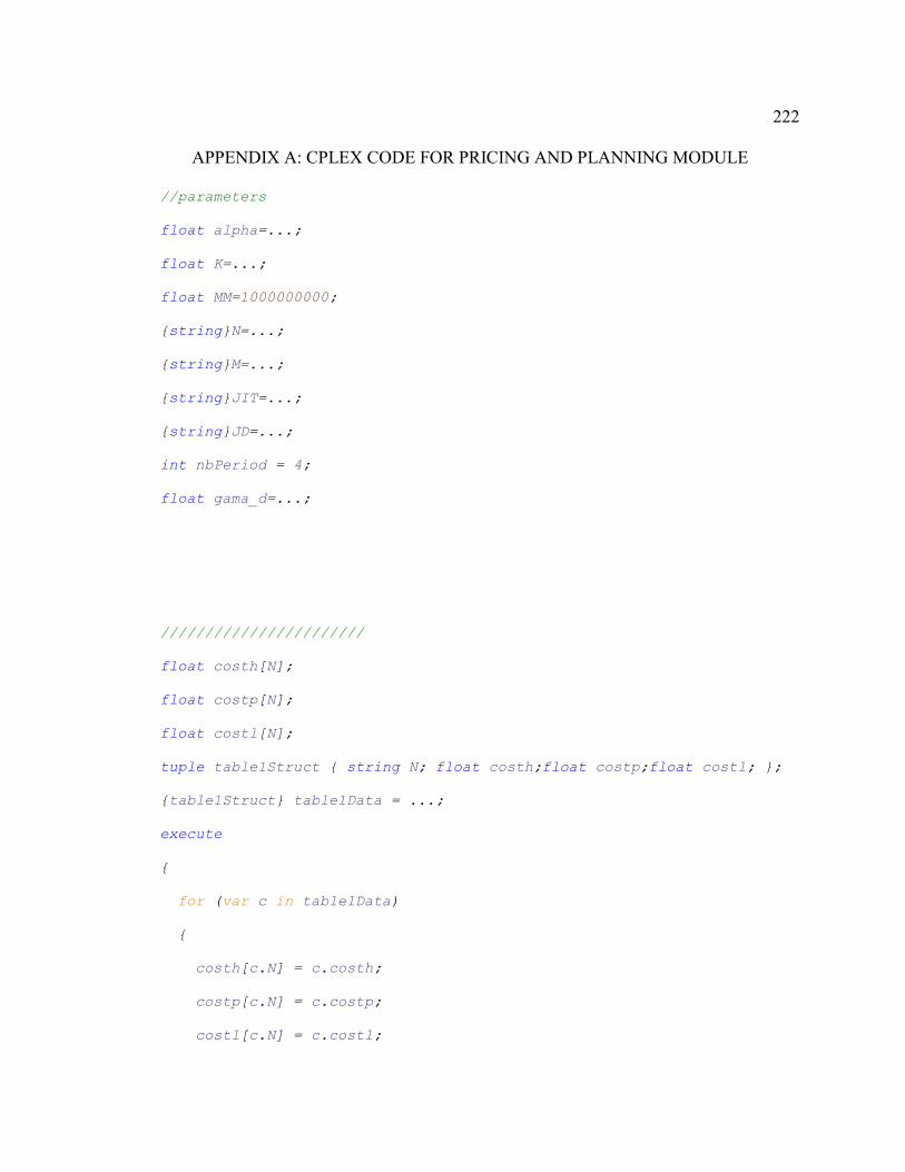
222

APPENDIX A: CPLEX CODE FOR PRICING AND PLANNING MODULE

//parameters

float alpha=...;

float K=...;

float MM=1000000000;

{string}N=...;

{string}M=...;

{string}JIT=...;

{string}JD=...;

int nbPeriod = 4;

float gama_d=...;

///////////////////////

float costh[N];

float costp[N];

float costl[N];

tuple table1Struct { string N; float costh;float costp;float costl; };

{table1Struct} table1Data = ...;

execute

{

for (var c in table1Data)

{

costh[c.N] = c.costh;

costp[c.N] = c.costp;

costl[c.N] = c.costl;

223 }

}

///////////////////////

float pu[N][1..nbPeriod];

float gama2[N][1..nbPeriod];

tuple table3Struct { string N;int period;float pu;float gama2; };


execute

{


{

pu[c.N][c.period] = c.pu;

gama2[c.N][c.period] = c.gama2;

}

}

///////////////////////

float lamda[N][M][1..nbPeriod];

float d_hat[N][M][1..nbPeriod];

float d_bar[N][M][1..nbPeriod];

tuple table4Struct { string N;string M; int period; float lamda;float

d_hat;float d_bar; };


execute

{


224 {

lamda[c.N][c.M][c.period] = c.lamda;

d_hat[c.N][c.M][c.period] = c.d_hat;

d_bar[c.N][c.M][c.period] = c.d_bar;

}

}

//variable

dvar boolean x[N][M][1..nbPeriod];

dvar boolean y[N][M][1..nbPeriod];

dvar float+ z[N][1..nbPeriod];

dvar float+ w[N][M][1..nbPeriod];

dvar float+ mio_hat[N][M][1..nbPeriod];

dvar float+ s[N][1..nbPeriod];

dvar float+ q[N][0..nbPeriod];

dvar float+ p[N][1..nbPeriod];

dvar float+ p2[N][JD][1..nbPeriod];

dvar float+ noo;

//model

maximize

225 sum(i in N,j in M, t in 1..nbPeriod)(w[i][j][t]*lamda[i][j][t]) -

sum(i in N, t in 1..nbPeriod)(costh[i]*q[i][t]) - sum(i in N, t in

1..nbPeriod)(costp[i]*p[i][t]) - sum(i in N,j in M, t in

1..nbPeriod)(costl[i]*x[i][j][t]*d_bar[i][j][t]) + sum(i in N,j in M, t

in 1..nbPeriod)(costl[i]*w[i][j][t])

- sum(i in N,j in JD, t in 1..nbPeriod)(mio_hat[i][j][t]) -

noo*gama_d;

subject to {

//////////////////////////////////////

forall(i in N, j in M, t in 1..nbPeriod)

q[i][t] - q[i][t-1] - p[i][t-1] + s[i][t-1]==0;

forall(i in N)

q[i][0]==0;

forall(i in N, t in 1..nbPeriod)

sum(j in M)x[i][j][t] == 1;


p[i][t]<=alpha * pu[i][t];

forall(t in 1..nbPeriod)

sum(i in N)(costp[i] * p[i][t]) <= K;

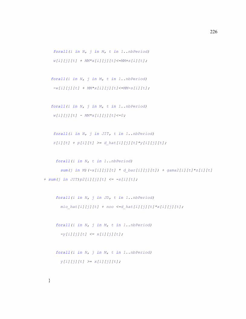
226


w[i][j][t] + MM*x[i][j][t]<=MM+s[i][t];


-w[i][j][t] + MM*x[i][j][t]<=MM-s[i][t];


w[i][j][t] - MM*x[i][j][t]<=0;

forall(i in N, j in JIT, t in 1..nbPeriod)

z[i][t] + p[i][t] >= d_hat[i][j][t]*y[i][j][t];


sum(j in M)(-x[i][j][t] * d_bar[i][j][t]) + gama2[i][t]*z[i][t]

+ sum(j in JIT)p2[i][j][t] <= -s[i][t];

forall(i in N, j in JD, t in 1..nbPeriod)

mio_hat[i][j][t] + noo <=d_hat[i][j][t]*x[i][j][t];


-y[i][j][t] <= x[i][j][t];


y[i][j][t] >= x[i][j][t];

}

227

APPENDIX B: SIMPLEX CODE USED IN PRICING AND PLANNING

MODULE

#include <stdio.h>

#include <math.h>

#define CMAX 10 //max. number of variables in economic function

#define VMAX 10 //max. number of constraints

int NC, NV, NOPTIMAL,P1,P2,XERR;

double TS[CMAX][VMAX];

void Data() {

double R1,R2;

char R;

int I,J;

printf("\n LINEAR PROGRAMMING\n\n");

printf(" MAXIMIZE (Y/N) ? "); scanf("%c", &R);

printf("\n NUMBER OF VARIABLES OF ECONOMIC FUNCTION ? ");

scanf("%d", &NV);

printf("\n NUMBER OF CONSTRAINTS ? "); scanf("%d", &NC);

if (R == 'Y' || R=='y')

R1 = 1.0;

else

R1 = -1.0;

printf("\n INPUT COEFFICIENTS OF ECONOMIC FUNCTION:\n");

for (J = 1; J<=NV; J++) {

228 printf(" #%d ? ", J); scanf("%lf", &R2);

TS[1][J+1] = R2 * R1;

}

printf(" Right hand side ? "); scanf("%lf", &R2);

TS[1][1] = R2 * R1;

for (I = 1; I<=NC; I++) {

printf("\n CONSTRAINT #%d:\n", I);

for (J = 1; J<=NV; J++) {

printf(" #%d ? ", J); scanf("%lf", &R2);

TS[I + 1][J + 1] = -R2;

}

printf(" Right hand side ? "); scanf("%lf", &TS[I+1][1]);

}

printf("\n\n RESULTS:\n\n");

for(J=1; J<=NV; J++) TS[0][J+1] = J;

for(I=NV+1; I<=NV+NC; I++) TS[I-NV+1][0] = I;

}

void Pivot();

void Formula();

void Optimize();

void Simplex() {

e10: Pivot();

Formula();

Optimize();

if (NOPTIMAL == 1) goto e10;

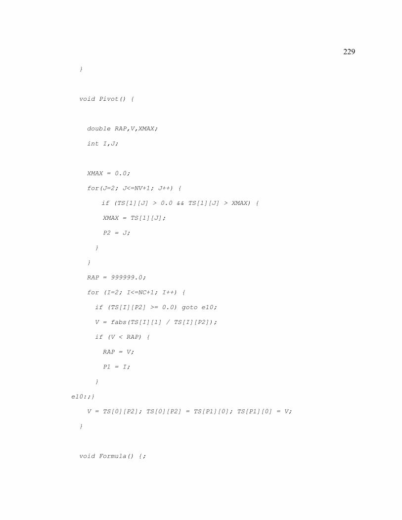
229 }

void Pivot() {

double RAP,V,XMAX;

int I,J;

XMAX = 0.0;

for(J=2; J<=NV+1; J++) {

if (TS[1][J] > 0.0 && TS[1][J] > XMAX) {

XMAX = TS[1][J];

P2 = J;

}

}

RAP = 999999.0;

for (I=2; I<=NC+1; I++) {

if (TS[I][P2] >= 0.0) goto e10;

V = fabs(TS[I][1] / TS[I][P2]);

if (V < RAP) {

RAP = V;

P1 = I;

}

e10:;}

V = TS[0][P2]; TS[0][P2] = TS[P1][0]; TS[P1][0] = V;

}

void Formula() {;

230 //Labels: e60,e70,e100,e110;

int I,J;

for (I=1; I<=NC+1; I++) {

if (I == P1) goto e70;

for (J=1; J<=NV+1; J++) {

if (J == P2) goto e60;

TS[I][J] -= TS[P1][J] * TS[I][P2] / TS[P1][P2];

e60:;}

e70:;}

TS[P1][P2] = 1.0 / TS[P1][P2];

for (J=1; J<=NV+1; J++) {

if (J == P2) goto e100;

TS[P1][J] *= fabs(TS[P1][P2]);

e100:;}

for (I=1; I<=NC+1; I++) {

if (I == P1) goto e110;

TS[I][P2] *= TS[P1][P2];

e110:;}

}

void Optimize() {

int I,J;

for (I=2; I<=NC+1; I++)

if (TS[I][1] < 0.0) XERR = 1;

NOPTIMAL = 0;

if (XERR == 1) return;

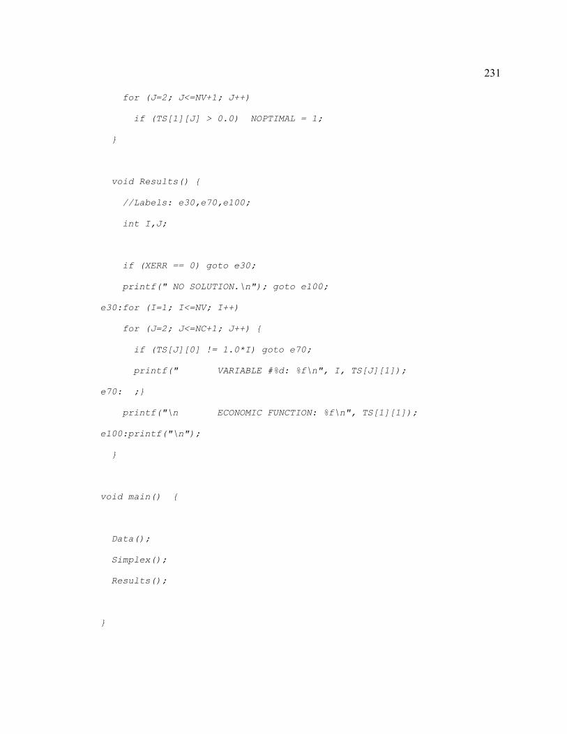
231 for (J=2; J<=NV+1; J++)

if (TS[1][J] > 0.0) NOPTIMAL = 1;

}

void Results() {

//Labels: e30,e70,e100;

int I,J;

if (XERR == 0) goto e30;

printf(" NO SOLUTION.\n"); goto e100;

e30:for (I=1; I<=NV; I++)

for (J=2; J<=NC+1; J++) {

if (TS[J][0] != 1.0*I) goto e70;

printf(" VARIABLE #%d: %f\n", I, TS[J][1]);

e70: ;}

printf("\n ECONOMIC FUNCTION: %f\n", TS[1][1]);

e100:printf("\n");

}

void main() {

Data();

Simplex();

Results();

}

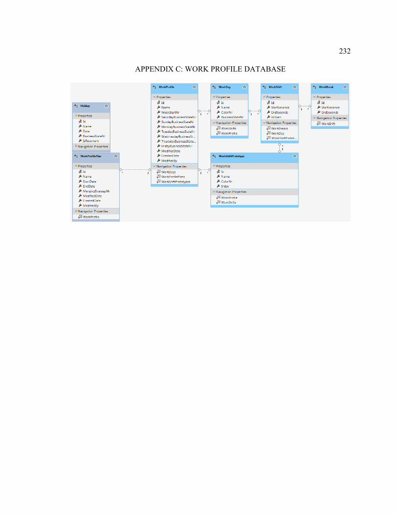
232

APPENDIX C: WORK PROFILE DATABASE

233

APPENDIX D: MACHINE AND MAINTENANCE DATABASE

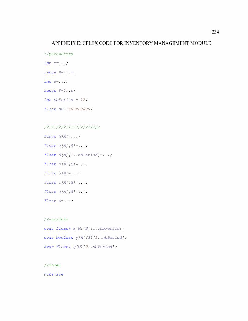
234

APPENDIX E: CPLEX CODE FOR INVENTORY MANAGEMENT MODULE

//parameters

int m=...;

range M=1..m;

int s=...;

range S=1..s;

int nbPeriod = 12;

float MM=1000000000;

///////////////////////

float h[M]=...;

float a[M][S]=...;

float d[M][1..nbPeriod]=...;

float p[M][S]=...;

float o[M]=...;

float l[M][S]=...;

float u[M][S]=...;

float W=...;

//variable

dvar float+ x[M][S][1..nbPeriod];

dvar boolean y[M][S][1..nbPeriod];

dvar float+ q[M][0..nbPeriod];

//model

minimize

235 sum(i in M,t in 1..nbPeriod)(h[i]*q[i][t]) + sum(i in M, j in S, t in

1..nbPeriod)(a[i][j]*y[i][j][t]) + sum(i in M, j in S, t in

1..nbPeriod)(p[i][j]*x[i][j][t]);

subject to {

//////////////////////////////////////

forall(i in M)

q[i][0]==0;

forall(i in M, t in 1..nbPeriod-1)

q[i][t+1] - q[i][t] - sum(j in S)x[i][j][t] + d[i][t]==0;

forall(t in 1..nbPeriod)

sum(i in M)o[i]*q[i][t]<=W;

forall(i in M, j in S, t in 1..nbPeriod)

l[i][j]*y[i][j][t]<=x[i][j][t];


x[i][j][t]<=MM*y[i][j][t];


x[i][j][t]<=u[i][j];

}

!!!!!!!!!!!!!!!!!!!!!!!!!!!!!!!!!!!!!!!

!!

Thesis and Dissertation Services

An Interactive Intelligent Decision Support System for ...

Documents

Transcript of An Interactive Intelligent Decision Support System for ...