1

An Index of Biotic Condition Based on Bird Assemblages in

Great Lakes Coastal Wetlands

Robert W. Howe1*, Ronald R. Regal2, JoAnn Hanowski2,

Gerald J. Niemi3 Nicholas P. Danz3 and Charles R. Smith4

1 Department of Natural and Applied Sciences

Cofrin Center for Biodiversity

University of Wisconsin-Green Bay

Green Bay, WI 54311-7001 2Department of Mathematics and Statistics,

University of Minnesota

Duluth, MN 55812

rregal@d.umn.edu

3Natural Resources Research Institute

University of Minnesota Duluth

Duluth, MN 55811-1442

jhanowsk@nrri.umn.edu, gniemi@d.umn.edu, ndanz@nrri.umn.edu 4Department of Natural Resources

Cornell University

Ithaca, NY 14853

crs6@cornell.edu

*Corresponding author. E-mail: hower@uwgb.edu.

2

ABSTRACT. We use bird distributions in non-forested coastal wetlands of the Great Lakes to

illustrate a new, conceptually explicit method for developing biotic indicators. The procedure

applies a probabilistic framework to derive an index that best “fits” an observed assemblage of

species, based on preliminary information about species’ responses to human environmental

disturbance. Among 215 coastal wetland complexes across the U.S. portion of the Great Lakes,

23 bird species were particularly sensitive (positively or negatively) to a multivariate

environmental disturbance gradient ranging from 0 (maximally disturbed) to 10 (minimally

disturbed). Species like Sandhill Crane and Sedge Wren showed strong negative relationships

with human disturbance, while others like Common Grackle, American Robin, and European

Starling, showed strong positive relationships with disturbance. The functional shapes of these

biotic responses were used to determine indices of biotic condition (IBC) for new sites. Values of

IBC were highly correlated with the environmental gradient, but deviations from a 1:1

relationship reveal novel insights about local ecological conditions. For example, sites

dominated by invasive plant species like Phragmites australis tended to yield IBC values that

were lower than expected based on environmental condition. This framework for calculating

biotic indicators holds significant potential for other applications because it is flexible, explicitly

linked to a disturbance gradient, and easy to calculate once standardized biotic response

functions are documented and made available for a region of interest.

KEY WORDS: indicator, coastal wetland, environmental assessment

3

INTRODUCTION

Coastal wetlands of the Laurentian Great Lakes provide important ecological links between

the lakes and surrounding watersheds. To a significant degree, the extent and health of those

coastal wetlands reflect the overall ecological condition of the coastal zone (Krieger et al. 1992).

Unfortunately, many of the Great Lakes’ coastal wetlands have been destroyed or degraded by

human activities (Herdendorf et al. 1981, Chow-Fraser and Albert 1999), in some cases leaving

only a small fraction of the original wetland area (Herdendorf 1987, Smith et al. 1991). Shoreline

development and invasive species, among other factors, continue to threaten remnant wetlands in

the Great Lakes coastal zone (Niemi et al. 2004).

To monitor ecosystem changes and to facilitate conservation strategies, biologists and

policy-makers have sought to develop quantitative indicators of ecosystem health for the Great

Lakes coastal zone (Shear et al. 2005). The State of the Lakes Ecosystem Conference (SOLEC)

was first convened in 1992 by U.S. and Canadian authorities to specifically address the reporting

requirements of the Great Lakes Water Quality Agreement of 1972 (Bertram et al. 2003).

Biannual meetings of SOLEC involving federal, state, provincial and local government agencies,

academic scientists, environmental groups, private industry, and the general public have led to

the publication of approximately 80 indicators, ranging from direct measures of toxic chemicals

in food webs to abundances of individual sensitive species (e.g., Hexagenia) or natural

communities (e,g, area, quality, and protection of alvar) to multivariate measures like the

diversity or abundance of wetland dependent bird species (Shear et al. 2005).

An ongoing challenge in the development of meaningful environmental indicators is an

understanding of relationships between indicators (e.g., diversity of wetland-dependent species)

and environmental stress (e.g., habitat degradation). Karr and Chu (1999), Jackson et al. (2000),

4

and others (Niemi and MacDonald 2004) provide conceptual frameworks for designing and

interpreting indicators of ecological health in relation to human activity. Those analyses are

important because they help guide the development of cost effective indicators and, most

importantly, because they can be used to help guide remedial actions for improving

environmental conditions.

In this paper we introduce the Index of Biotic Condition (IBC), a new approach for

developing ecological indicators. The general method (Howe et al. 2007) uses a probabilistic

framework pioneered by Hilborn and Mangel (1997) to assess the occurrences of species (or any

set of monotonic variables) in the context of an explicit gradient of environmental stress or

disturbance. This flexible approach can use either simple biological variables like those used in

the Hilsenhoff (1982) Index and its analogues or multimetric variables like those used in the

Index of Biotic Integrity (IBI) of Karr (1981) and others. Our approach is unique because of the

way in which the final number (index) is generated.

The IBC approach, like the multimetric approach of Karr (1981), requires that users

clearly identify an independent environmental gradient, which ultimately helps determine what

the biotic indicator truly “indicates.” As long as the same preliminary environmental gradient is

applied, estimates from different taxonomic groups, different types of variables, and even

different field methods can be compared and combined readily because information from

different species or variables is not additive.

Application of our method requires that preliminary studies or expert opinion quantify the

responses of species or other variables to an explicit environmental stress or disturbance

gradient, which we will simply call the environmental gradient. Points along the environmental

gradient will be defined as having an environmental condition of Cenv. Once the responses of

5

species to the environmental gradient have been documented, users provide data on the

occurrences of species or values of the response variables at new places of interest. The Index of

Biotic Condition is calculated iteratively using widely available computer software (e.g.,

Microsoft Excel), leading to an estimate of ecological condition ranging from 0 (maximally

degraded) to 10 (minimally degraded). Conceptually, we suggest that this approach measures

ecological condition because it combines biotic condition (as calculated by the quantitative IBC)

and environmental condition (as defined by the original environmental gradient).

We illustrate the Index of Biotic Condition by applying results from an extensive survey

of birds in coastal wetlands of the U.S. portion of the Laurentian Great Lakes. Our purpose is

not to seek the final word on bird-related indicators in this system. Instead, we use this

information to demonstrate the method and to provide a foundation for later, more complete

analyses of coastal wetland bird assemblages and their suitability as ecological indicators.

Probability Indicator Model

Consider the probability of observing a particular species, ( )iP C , given an ecological

condition, C, at a specific site. For simplicity, we define a fixed scale of 0 < C < 10, where 0

represents the most degraded condition and 10 represents the most pristine or desirable

condition. The probability of observing species i can be described by a function of the site’s

condition and p attributes β = βi,1, ...,β ip, which reflect the species’ response to variation in

ecological condition. The height of the response curve along the gradient (i.e., its position on the

y-axis) will reflect the species’ overall ubiquity in the region and its ease of detection. We call

this quantitative relationship a biotic response (BR) function, identical to the species-specific

sensitivity/detectability (SSD) functions described by Howe et al. (2007). The function is

6

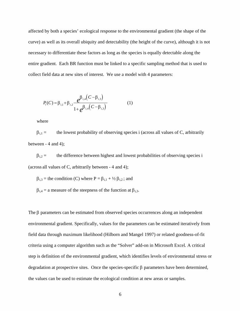
affected by both a species’ ecological response to the environmental gradient (the shape of the

curve) as well as its overall ubiquity and detectability (the height of the curve), although it is not

necessary to differentiate these factors as long as the species is equally detectable along the

entire gradient. Each BR function must be linked to a specific sampling method that is used to

collect field data at new sites of interest. We use a model with 4 parameters:

( )

( ),4 ,3

,1 ,2,4 ,3

( )1

i i

i i ii i

CP C

Cee

−β β= +β β

−β β+ (1)

where

βi,1 = the lowest probability of observing species i (across all values of C, arbitrarily

between - 4 and 4);

βi,2 = the difference between highest and lowest probabilities of observing species i

(across all values of C, arbitrarily between - 4 and 4);

βi,3 = the condition (C) where P = βi,1 + ½ βi,2 ; and

βi,4 = a measure of the steepness of the function at βi,3.

The β parameters can be estimated from observed species occurrences along an independent

environmental gradient. Specifically, values for the parameters can be estimated iteratively from

field data through maximum likelihood (Hilborn and Mangel 1997) or related goodness-of-fit

criteria using a computer algorithm such as the “Solver” add-on in Microsoft Excel. A critical

step is definition of the environmental gradient, which identifies levels of environmental stress or

degradation at prospective sites. Once the species-specific β parameters have been determined,

the values can be used to estimate the ecological condition at new areas or samples.

7

Separate BR functions are modeled for each species (or each variable), representing

different species’ (or variable) responses to ecological condition. Some species or variables may

show negative responses to environmental stress (Figures 1a-1d), while others may show a

positive response (Figures 1e and 1f). The height of the response curve along the vertical axis is

associated with the species’ overall relative abundance and ease of detection or, in the case of

other variables, the scale of magnitude of each variable. The β parameters are fixed constants for

an area or region of interest, although different species-specific functions might be applied for

different habitat types, different field methods, or different climatic conditions (e.g., different

water level regimes in the Great Lakes (Wilcox et al. 2002)).

To derive the species-specific BR functions, the environmental gradient must be defined a

priori. Sites with ideal condition (i.e., Cenv = 10) or maximally degraded condition (i.e., Cenv = 0)

might not exist in nature, but the investigator nevertheless must model the expected probabilities

of occurrence under these conditions.

The Index of Biotic Condition (an estimate of C) is calculated by applying the BR functions

to standardized field data, acquired using the same methods that generated the BR functions. An

iterative computer program asks the mathematical question: “Given the a priori BR functions,

what is the value of C that best fits the observed field data?” In our examples the BR functions

describe probabilities of species’ occurrences (ranging between 0 and 1), but any variable that

changes monotonically over the environmental gradient can be used. C can be estimated in two

ways: 1) a least squares method, which finds the value of C that minimizes the sum of squared

differences between expected probabilities of species presence, Pi(Ci) and observed

probabilities of presence, pi, for i = 1, 2, …, n species, and 2) a likelihood method, which finds

the value of C that maximizes

8

( ) ( )log ( ) log 1 ( )i iobserved unobserved

P C P C+ −∑ ∑ (2)

where the term on the left is the sum of log-probabilities of species that were observed at the site

and the term on the right is the sum of log-probabilities of species that were not observed. In

cases like ours, the observed probabilities (pi) are the proportions of field samples in which

species i was detected. The likelihood method is applicable where multiple samples are

available for a given site or category of sites. If targeted sites have many species characteristic

of high quality environmental condition (e.g., Cenv > 7) and few species characteristic of poor

conditions (e.g., Cenv < 3), the site will yield a high estimate of C; if the sites have few species

associated quality environmental condition and many species associated with poor condition, the

site is will yield a low estimate of C. A computer algorithm like Microsoft Excel’s “Solver” can

be used to find the best-fit value of C.

This approach assumes that species respond in various ways to a common gradient of

ecological condition. For a given location our Index of Biotic Condition reflects the BR

functions of all species simultaneously. To avoid spurious estimates of C, the analysis can be

restricted to species showing strong statistical responses to stress (i.e., steep BR functions with

minimal scatter) or to species characteristic of a particular habitat type.

METHODS

We applied our probabilistic indicator approach to samples of breeding birds from 215

wetland complexes in the U.S. portion of the Great Lakes (Figure 2) during 2002 and 2003

(Table 1). Wetland complexes consisted of one or more non-forested coastal wetlands (marshes

or shrub wetlands) located within the same local drainage area, ranging from 1 to 1265 ha

(average = 91 ha) and within 1 km of the Great Lakes shoreline. We sampled a variety of

9

wetland types (Albert et al. 2003), including riparian wetlands, coastal marshes, and protected

wetlands not directly connected to the lake. Wetland complexes were selected according to a

stratified random method described by Danz et al. (2005). The number of bird sample points

varied from only a single point in the smallest wetlands (65% of wetland complexes), two points

in 47 moderately large complexes (22%), three points in 26 larger complexes (12%), and 4 and 5

points in the two largest complexes. Sampling was conducted during both 2002 and 2003 at 50

of the 321 sample points, giving a total of 371 point samples. Differences in bird distributions

between the two years were minor, so we treated each point count as a separate sample.

From each bird survey point, field observers recorded all birds seen or heard within a 100 m

radius half-circle extending from the edge into the wetland. This method and standardized data

forms followed the standardized National Marsh Monitoring Protocol (Ribic et el. 1999). All

point counts were conducted between first light (just before sunrise) and 9:00 a.m. in benign

weather conditions (rainless with winds < 20 km/h). Field samples were part of the

multidisciplinary Great Lakes Environmental Indicators project (GLEI) funded by the U.S.

Environmental Protection Agency (http://glei.nrri.umn.edu).

A large suite of independent environmental variables was acquired by GLEI collaborators

for each of the wetland complexes (Table 2). One set of variables (1-8 in Table 2) applies to the

drainage area of the shoreline segment (segment-shed) associated with the wetland complex.

Danz et al. (2006) used principal components analysis (PCA) to summarize of 5 groups of

anthropogenic variables, including agricultural data, pesticide application records, point sources

of chemical and air pollution, soil attributes, and human population density. A second set of

variables (9-39 in Table 2) was derived from Landsat 5 and Landsat 7 satellite imagery (30 m x

30 m pixels) from the years 1992 and 2001 (Wolter et al. 2006). Land cover classes were

10

combined into 6 general categories (Table 2). ArcGis 9.1 (ESRI 2005) was used to calculate the

proportional area of each land cover category within 100 m, 500 m, 1 km, and 5 km of the

centroid of the wetland complex. Principal Components Analysis (correlation matrix) was used

to further summarize these 39 environmental variables (Table 2). Scores from the resulting

principal components were combined into a single index of human impact (= Cenv), forming a

standardized environmental gradient. Cenv was calculated for each wetland complex by adding

the scores for each principal component accounting for at least 5% of the overall variation,

weighted according to the percent variation explained. This analysis allowed us to order the

wetland complexes along a single environmental gradient, ranging from most impacted sites

(e.g., sites with high levels of pesticide application, high air pollution emissions, high human

population density, low proportion of natural vegetation or wetland land cover, many roads, etc.)

to least impacted sites.

The gradient of environmental condition (Cenv) among sampled wetlands was used to

develop biotic response (BR) functions for bird species. Wetland sites were grouped into 20

categories of 0.5 units (0.00 – 0.49, 0.5 – 0.99, 1.00 – 1.49,.., 9.5-10.0) ranging from maximally

stressed or affected by human activities (C = 0) to minimally impacted (C = 10). For species i and

category j the proportion pij was defined as the proportion of bird sample points where the

species was recorded. Parameters of the best-fit BR functions were estimated by iteration,

minimizing the expression:

1

N

j=∑ (pij – Pi(Cj))2/( Pi(Cj)*(1- Pi(Cj))) (3)

11

where N, equal to 20 here, is the total number of samples (in this case, categories), pij is the

observed proportion of point samples in category j where observers detected species i, Cj is the

midpoint value of C in the jth interval (e.g., 0.25 for the interval 0.0 – 0.49), and Pi(Cj) is the

expected probability of occurrence from equation 1 given a specific set of parameter values for

the BR function. The “Solver” tool of Microsoft Excel was used to derive parameter estimates

for βi,1, βi,2 , βi,3 and βi by minimizing Equation 3, subject to the constraints that 0 < βi,1 <1, 0 <

βi,2 < 1-βi,1, and 0 < Pi(Cj) < 1. We also limited the steepness parameter (βi,4) to values between -

1 and 1.

We tested this method by evaluating birds at 20 wetland complexes that were randomly

excluded (“reserved”) from the development of BR functions. Indexes of Biotic Condition based

on bird species composition were derived using the maximum likelihood method of estimation.

Bird species selected for the calculations had BR functions that met the following criteria: 1) the

absolute difference between the predicted probability of occurrence at C = 10 and C = 0 was at

least 0.2 (in other words, the species showed strong sensitivity to condition, either positively or

negatively); and 2) the lack-of-fit (LOF) expression (Equation 3) was less than 1.75, thereby

excluding species that showed relatively high scatter around the BR function. We also excluded

colonial species like Great Blue Heron (Ardea herodias), forest specialists like Red-eyed Vireo

(Vireo olivaceus), and aerial feeders like Northern Rough-winged Swallow (Stelgidopteryx

serripennis) and Barn Swallow (Hirundo rustica) because their presence in a coastal wetland is

largely dependent on proximity to habitats or local nesting sites that are not part of the wetland

complex. Results (IBC’s) were compared with the independently-derived estimates of

environmental condition (Cenv) for each wetland complex.

12

RESULTS

Principal components analysis (PCA) of environmental variables yielded 5 interpretable

axes of variation among wetland complexes, together accounting for 68% of the variance in the

original 39 environmental variables. Principal component 1, associated with 24.3% of the

variation, was most strongly correlated (negatively) with the proportion of natural vegetation

within 500 m of the wetland complex centroid (Figure 3a); other correlated variables included

proportions of natural vegetation at 100 m, 1 km, and 5 km and proportions of wetland

vegetation within 100 m and 5 km. Positive correlates with principal component 1 included

proportion of residential land cover within 500 m and 5 km (Figure 3b) and total road length

within 5 km. The second principal component, accounting for 17.4% of the overall variation,

was strongly correlated with proportions of cultivated land at all distances (Figure 3c) and the

multivariate index (principal component) of agricultural activity defined by Danz et al. (2006).

Proportions of natural vegetation (especially within 500 m and 1 km) were negatively associated

with principal component 2. The third principal component, accounting for 13.3% of the

variation, separated sites with extensive wetland area from sites with predominately upland

vegetation (Figure 3d), including residential, natural, and cultivated lands. The fourth principal

component, accounting for 7.4% of the variation, was negatively correlated with industrial land

cover types and positively correlated with residential land use. Finally, the fifth principal

component, accounting for 5.7% of the variation, was negatively correlated with the proportion

of natural vegetation within and near the wetland complex itself, and positively correlated with

road length and proportion of road associated land cover in the vicinity (< 500 m) of the wetland

13

complex. In all of these cases, the principal components differentiated sites that were heavily

influenced by human activities from sites that were less influenced.

The PCA scores were combined by 1) reversing the signs of Axes 1,2,3 and 5 so that all

scores correlated with a gradient from maximally degraded to minimally degraded sites; 2)

converting the PCA scores to a standardized scale (0 – 10); and 3) weighting the standardized

scores by the % total variation associated with the corresponding PCA axis. The 5 adjusted

scores then were summed to give a single gradient of environmental condition (Cenv), ranging

from 0 (maximally degraded) to 10 (minimally degraded). Values along this environmental

gradient were highest for wetland complexes with high proportions of natural and wetland

vegetation surrounding the wetland and lowest for complexes with a high proportion of

urban/industrial lands and extensive roads within and near the wetland complex.

From 155 bird species observed at least once in our study sites, we selected 23 wetland,

shrub/woodland, or open country species (Table 3) that exhibited relatively strong sensitivity to

the reference gradient (|P(C(10)-P(C(0)| > 0.20) and relatively low deviation from the best-fit BR

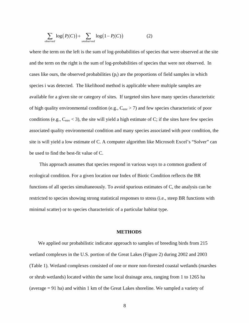
function (LOF < 1.75). Swamp Sparrow, Common Yellowthroat (Figure 1a), Sandhill Crane

(Figure 1b), and Sedge Wren showed strongest positive associations with the reference gradient

(β2 >> β1 and β4 > 0), while Common Grackle (Figure 1e), American Robin, European Starling,

Northern Cardinal, and Mallard (Figure 1f), showed strongest negative relationships (β2 > β1 and

β4 < 0). The shapes of the best-fit BR functions varied according to the ecology and overall

abundance of different species. Bald Eagle, for example, showed a rather low probability of

occurrence even at pristine wetland complexes (Figure 1c), whereas Swamp Sparrow exhibited a

positive relationship with environmental condition but was present at even some highly degraded

sites (Figure 1d).

14

Given parameters from the best-fit biotic response (BR) functions (Table 3) and detection

data for the 23 selected bird species, we used the “Solver” function of Microsoft Excel to

estimate ecological condition (Index of Biotic Condition) for the 20 reserved sites. The resulting

IBC’s (Figure 4a) correspond closely to the independently derived Cenv based on environmental

variables (r = 0.77, p < 0.01), showing that bird species composition of coastal wetlands can

meaningfully indicate ecological condition. Deviations from a 1:1 relationship between the Index

of Biotic Condition and Cenv are especially meaningful. In at least two cases (Point au Sauble on

Lake Michigan/Green Bay and near the mouth of the Calumet River in Indiana), the Index of

Biotic Condition was substantially lower than Cenv (e.g.,) at wetlands with extensive cover of

invasive species, especially common reed, Phragmites australis, and purple loosestrife, Lythrum

salicaria.

DISCUSSION

The advantages of using species as environmental indicators have been articulated

extensively by Karr (1981), McGeoch and Chown (1998), Yoder and Rankin (1998), Karr and

Chu (1999), O’Connor et al. (2000), Niemi and McDonald (2005) and others. (But see Landres

et al. (1988) for an alternative perspective.) Species assemblages integrate the effects of

environmental stress over space and time and populations of sensitive species represent

biologically meaningful signals from many interacting and complex variables.

Results of our analysis show that birds of coastal wetlands are differentially sensitive to

environmental condition. Some species are associated positively with human impacts, others are

associated negatively, while others show no consistent, monotonic relationship. The first two

groups (sensitive species) can be used as indicators of a site’s ecological condition.

15

The relationship between our empirically-derived biotic condition (IBC) and environmental

condition (Cenv), however, is not 1:1. For example, a wetland near Green Bay, Wisconsin (Pt. au

Sauble) showed an environmental condition (Cenv) of 4.87, but the bird-based IBC was only 2.05

(Figure 4a). This wetland was dominated by the invasive plant Phragmites australis, which was

not reflected in the land cover and land use variables used to calculate Cenv. Consequently, the

observed bird species composition indicated a lower level of ecological condition than predicted

by the environmental variables. In this and other cases, the IBC provided more information

about the site’s condition than environmental variables alone. This finding also suggests that a

more detailed environmental gradient that takes into account invasive species should be used in

the derivation of biotic response (BR) functions. As more information is acquired about Great

Lakes Coastal wetlands and their biota, improvements in the BR functions and in IBC values for

individual wetlands will be desirable.

With two exceptions (both from Lake Ontario) wetlands with low values of environmental

condition (Cenv < 0.6) tended to yield even lower values of biotic condition (IBC), suggesting that

a threshold effect might apply to bird species composition (Figure 4). In other words, highly

sensitive bird species occur especially infrequently (or highly tolerant species occur especially

frequently) below a certain level of environmental degradation (e.g. Cenv < 0.6). The nonlinear

forms of many BR functions further illustrate this view (Figure 1). If verified by further analyses,

this finding has important implications for conservation of Great Lakes environmental quality

and possibly for wetlands in other geographic areas. To sustain environmentally sensitive bird

species, natural vegetation and other aspects of landscape quality must be maintained at or above

threshold levels, in our case corresponding to Cenv values higher than 6.0. In general, species like

Sandhill Crane, Bald Eagle, and Sedge Wren were absent from sites with environmental

16

condition below this threshold level, even though they would have been expected to occur at

least occasionally.

Calculation of the Index of Biotic Condition requires three steps: 1) definition of a standard

environmental gradient ranging from 0 (poorest condition) to 10 (best condition); 2)

development of BR functions describing species’ responses (or responses of some other variable)

to the environmental gradient; and 3) iterative calculation of the best-fit Index of Biotic

Condition given field data for a site of interest. Steps 1 and 2 are data intensive and typically

require large scale analyses such as our comprehensive surveys of birds in the Great Lakes Basin

(Niemi et al. 2006). As new information is accumulated, the environmental gradient and BR

functions can be improved and applied to both new and old data sets. Ideally, managers and

scientists will establish standard gradients and BR functions, enabling widespread comparisons

among sites over time and space. Note that different BR functions can be developed for different

sampling methods or for different habitat types. As long as the same environmental gradient is

used as a baseline the resulting Indices of Biotic Condition (ranging from 0 to 10) will be

comparable. The key consideration is that methods used to acquire field data at the target sites

are identical to the methods used to derive the applicable BR functions. Field data for animal or

plant species may consist of either probabilities of occurrence (e.g., frequency of presence in

multiple samples) or presence/absence in single samples. If probabilities of occurrence are

available, then the least squares method is used to estimate IBC’s; if only presence/absence data

are available, then the maximum likelihood method is used. A Microsoft Excel spreadsheet is

available from the authors with instructions and framework for calculating both BR functions

and IBC’s.

17

The pre-defined environmental gradient represents a first attempt to characterize ecological

condition at specific sites, but a species-based index (IBC) provides additional information about

environmental quality and in most cases provides a less expensive and conceptually simpler

method of site assessment. Although the IBC is useful as a standalone measure of ecological

condition, comparison of a site’s IBC and Cenv may provide additional insights into the locality’s

condition. Sites with higher than expected IBC might possess favorable attributes that are worth

emulating elsewhere; sites with lower than expected IBC might harbor unrecognized

environmental problems that deserve attention.

We have provided a preliminary set of BR functions (Table 3) that can be used by land

managers and others to characterize the ecological condition of coastal wetlands in the U.S.

portion of the Great Lakes. Our primary goal in this paper, however, is to introduce the IBC

approach with a specific example. Further research and analysis of existing data should refine

the BR parameters for broader use. In particular, we encourage the addition of multi-species

variables that will take into account rarer species like rails, raptors, and other water birds. For

example, a useful variable might be the probability of observing any one of several rare species.

A biotic response (BR) function can be fitted for such multi-species variables just as we have

done here for individual species.

The Index of Biotic Condition achieves similar objectives as the Index of Biotic Integrity

(IBI) introduced by Karr (1981) and applied by Harris and Silviera (1999), Butcher et al. (2003),

Crewe and Timmermans (2005), and many others. In the example presented here we use only

single species variables rather than multispecies or community level variables, but IBC

calculations can employ both single species and multispecies variables. The major difference

between the IBC and IBI approaches is the way in which variables are combined. In the IBC an

18

iterative, probabilistic framework articulated by Hilborn and Mangel (1997) is used to estimate

the IBC value that best fits an observed data set. All applications of the IBC approach use a

standard range between 0 (poorest condition) to 10 (best condition). In the IBI approach,

variables are converted to a standardized range of values (e.g., 1,3, or 5) and summed, leading to

different scale of IBI values depending on the number of variables used in the analysis. Other

approaches such as the floristic quality index (Wilhelm and Ladd 1988) and RIVPACS methods

(Wright et al. 1993) use species richness or taxonomic richness (ratio of observed / expected

taxa). Both of these methods are sensitive to sampling area or sampling effort, and neither

method documents the relationship between species occurrences or taxonomic richness variables

and an explicit environmental gradient. In the IBC approach, users are required to identify BR

functions (perhaps generated by previous investigators) that clearly document the sensitivity of

species or variables to an environmental gradient. This requirement insures that species or

variables with different responses to disturbance are not treated identically. The IBC approach

also provides a more transparent understanding of exactly what the indicator is meant to indicate.

Because it uses a standard 0 to 10 scale, the IBC method can incorporate data from different

taxonomic groups or even different sampling methods as long as standardized BR functions are

based on the same environmental gradient. Walsh (2006) argued that assessment of indicators

against a standard disturbance gradient is critical for application of management objectives. Our

approach requires that such an environmental gradient is pre-defined and built into the IBC

process. Calculation of IBC values for sites of interest is straightforward and flexible once users

have agreed on an underlying gradient.

Our method can be applied to any habitat or geographic area of interest. In order for IBC

values to be valid, of course, different biotic response (BR) functions need to be calculated for

19

different habitats, different sampling methods, and perhaps different regions. Variation in biotic

responses of a single species among different geographic areas is poorly known and represents

an interesting subject in its own right. We envision the development of standard BR functions to

be completed by large scale studies involving scientists from government agencies, universities,

industry, and organizations. Once these functions have been standardized, managers can apply

the IBC method at individual localities within the appropriate region.

ACKNOWLEDGMENTS

This research was supported by a grant from the U.S. Environmental Protection Agency’s

Science to Achieve Results Estuarine and Great Lakes program through funding to the Great

Lakes Environmental Indicators project, U.S. EPA Agreement EPA/R-8286750 and a grant from

the National Aeronautics and Space Administration (NAG5-11262). This document has not been

subjected to U.S. EPA required peer and policy review and therefore does not necessarily reflect

the views of the Agency, and no official endorsement should be inferred. We are grateful for

contributions by other scientists involved with the GLEI project, especially T. Hollenhorst, P.

Wolter, V. Brady, T. Brown, J. Brazner, S. Price, D. Marks, and others, including more than 20

student field investigators. Important ideas underlying this analysis were communicated by J.

Karr, D. Simberloff, P. Bertram, A. Tyre, and H. Possingham. This is contribution number xxx

of the Center for Water and the Environment, Natural Resources Research Institute, University

of Minnesota Duluth.

20

REFERENCES

A.O.U. 1998. Check-list of North American birds, 7th ed. Washington, DC: American

Ornithologists’ Union.

Albert, D.A., Ingram, J., Thompson, T. Wilcox, D. 2003. Great Lakes coastal wetlands

classification. Great Lakes Coastal Wetland Consortium.

http://www.glc.org/wetlands/pdf/wetlands-class_rev1.pdf.

Bertram, P., Stadler-Salt, N., Horvatin, P., and Shear, H. 2003. Bi-national assessment of the

Great Lakes - SOLEC partnerships. Environ. Monit. Assess. 81(1-3): 27-33.

Butcher, J.T., Stewart, P.M., and Simon, T.P. 2003. A benthic community index for streams in

the northern lakes and forests ecoregion. Ecol. Indicators 3:181-193.

Chow-Fraser, P. and Albert, D. 1999. Identification of eco-reaches of Great Lakes coastal

wetlands that have high biodiversity values. Discussion paper for SOLEC 1998. Env

Canada-U.S. EPA Publications.

Crewe, T.L., and Timmermans, S.T.A. 2005. Assessing biological integrity of Great Lakes

coastal wetlands using marsh bird and amphibian species. Wetland 3-EPA-01 Technical

report. Marsh Monitoring Program, Bird Studies Canada.

Danz, N., Regal, R., Niemi, G.J., Brady, V.J., Hollenhorst, T., Johnson, L.B., Host, G.E.,

Hanowski, J.M., Johnston, C.A., Brown, T., Kingston, J., and Kelly, J.R. 2005.

Environmentally stratified sampling design for the development of Great Lakes

environmental indicators. Environ. Monit. Assess. 102:41-65.

_____ , Niemi, G.J., Regal, R.R., Hollenhorst, T., Johnson, L.B., Hanowski, J.M., Axler, R.J.,

Ciborowski, J.H., Hrabik, T., Brady, V.J., Kelly, J.R., Brazner, J.C., Howe, R.W., Johnston,

21

C.A., and Host, G.E. 2006. Integrated gradients of anthropogenic stress in the U.S. Great

Lakes basin. Environ. Manage. In press.

ESRI. 2005. ArcGIS 9.1. Redlands, CA: Environmental Systems Research Institute.

Harris, J.H., and Silviera, R. 1999. Large-scale assessments of river health using an index of

biotic integrity with low-diversity fish communities. Freshw. Biol. 41, 235–252.

Herdendorf, C.E., Hartley, S.M., and Barnes, M.D.eds. 1981a. Fish and wildlife resources of the

Great Lakes coastal wetlands within the United States, Vol. 1: Overview. U.S. Fish and

Wildlife Service, FWS/OBS-81/02-v1.

_____ . 1987. The ecology of coastal marshes of western Lake Erie: a community profile. U.S.

Fish and Wildlife Service, Biological Report 85(7.9), 240 pp.

Hilborn, R., and Mangel, M. 1997. The ecological detective: confronting models with data.

Princeton, New Jersey: Princeton University Press

Hilsenhoff, W. L. 1982. Using a biotic index to evaluate water quality in streams. Techn. Bull.

132, WI Dept. Nat. Res., Madison WI.

Howe, R.W., Regal, R.R., Niemi, G.J., Danz, N.P., and Hanowski, J.M. 2006. A probability-

based indicator of ecological condition. Ecol. Indicators. In press.

Jackson, L.E., Kurtz J.C., and Fisher W.S., eds. 2000. Evaluation guidelines for ecological

indicators. Research Triangle Park. NC: U.S. Environmental Protection Agency, Office of

Research and Development. EPA/620/R-99/005. 107 p.

Karr, J. R. 1981. Assessment of biotic integrity using fish communities. Fisheries 6:21-27.

_____ , and Chu, E.W. 1999. Restoring life in running waters: better biological monitoring.

Washington, DC: Island Press.

22

Krieger, K.A., Klarer, D.M., Heath, R.T., and Herdendorf C.E. 1992. Coastal wetlands of the

Laurentian Great Lakes: current knowledge and research needs. J. Great Lakes

Res.18(4):525-528.

Landres, P.B., Verner, J., and Thomas, J.W. 1988. Ecological uses of vertebrate indicator

species: a critique. Conserv. Biol. 2(4):316-328.

McGeoch, M.A., and Chown, S.L. 1998. Scaling up the value of bioindicators. Trends Ecol.

Evolut. 13:46-47.

Niemi, G.J., and McDonald, M. 2004. Application of ecological indicators. Ann. Rev. Ecol. Syst.

35:89-111.

_____ , Wardrop, D., Brooks, R., Anderson, S., Brady, V., Paerl, H., Rakocinski, C., Brouwer,

M., Levinson, B., and McDonald, M. 2004. Rationale for a new generation of ecological

indicators for coastal waters. Environ. Health Persp. 112:979-986.

O'Connor, R.J., Walls, T.E., and Hughes, R.M. 2000. Using multiple taxonomic groups to index

the ecological condition of lakes. Environ. Monit. Assess. 61, 207-28.

Ribic, C.A., Lewis, S. J., Melvin, S., Bart, J., and Peterjohn, B. 1999. Proceedings of the Marsh

Bird Monitoring workshop. U.S. Fish and Wildlife Service, U.S. Geological Survey.

Shear, H., Bertram, P., Forst, C., and Horvatin, P. 2005. Development and application of

ecosystem health indicators in the North American Great Lakes basin. In A handbook of

ecological indicators for assessment of ecosystem health, eds., S.E. Jorgensen, R. Costanza,

F.-L. Xu, pp. 105-126.

Smith, P.G.R., Glooschenko, V., and Hagen, D.A. 1991. Coastal wetlands of the three Canadian

Great Lakes: inventory, current conservation initiatives and patterns of variation. Can. J.

Fish. Aquat. Sci. 48:1581-1594.

23

Walsh, C.J. 2006. Biological indicators of stream health using macroinvertebrate assemblage

composition: a comparison of sensitivity to an urban gradient. Marine and Freshwater

Research 57:37-47.

Weeber, R.C., and Vallianatos, M., eds. 2000. The Marsh Monitoring Program 1995 – 1999:

monitoring great lakes wetlands and their amphibian and bird inhabitants. Bird Studies

Canada, in cooperation with Environment Canada and the U.S. Environmental Protection

Agency. 47 pp.

Wilcox, D.A., Meeker, J.E., Hudson, P.L., Armitage, B.J., Black, M.G., and Uzarski, D.G. 2002.

Hydrologic variability and the application of index of biotic integrity metrics to wetlands: a

Great Lakes evaluation. Wetlands 22:588-615.

Wilhelm, G S., and Ladd, D. 1988. Natural area assessment in the Chicago region. Proc. N. Am.

Wildlife Natural Resources Conf. 53:361-375.

Wolter, P.T., Johnston, C.A., and Niemi, G.J. 2006. Land use change in the U.S. Great Lakes

basin 1992-2001. J. Great Lakes Res. 32:607-628.

Wright, J.F., M.T. Furse, and P.D. Armitage. 1993. RIVPACS – a technique for evaluating the

biological quality of rivers in the U.K. European Water Pollution Control 3:15-25.

Yoder, C.O., and Rankin, E.T. 1998. The role of biological indicators in a state water quality

management process. J. Environ. Mon. Assess. 51:61-88.

24

TABLE 1. Distribution of sampling points among Great Lakes and coastal segments, defined

as the drainage area associated with major rivers and streams (Danz et al. 2005).

Lake Segments Points

Erie 24 41

Huron 47 61

Michigan 73 113

Ontario 35 61

Superior 45 62

Total 224 338

25

TABLE 2. Variables used to define an environmental stress gradient associated with wetland

bird survey sites. Principal components incorporate numerous variables derived from the

drainage area of the shoreline segment (segment-shed) surrounding the wetland complex

(Danz et al. 2006). Land cover classes were determined by Wolter and others at the University

of Minnesota Duluth’s Natural Resources Research Institute (Wolter et al. 2006) and

combined into 6 general categories (industrial, roads, residential, cultivated, natural, wetland).

Proportions of land cover in each category were determined by GIS analysis for areas within

100 m, 500 m, 1 km, and 5 km of the centroid of the wetland complex.

Variable #(s) Variable(s) 1 Agricultural principal component 1 (Danz et al. 2006) 2 Atmospheric deposition principal component 1 (Danz et al. 2006) 3 Atmospheric deposition principal component 2 (Danz et al. 2006) 4 Point source pollution principal component 1 (Danz et al. 2006) 5 Point source pollution principal component 2 (Danz et al. 2006) 6 Soil type principal component 1 (Danz et al. 2006) 7 Soil type principal component 1 (Danz et al. 2006) 8 Urbanization principal component 1 (Danz et al. 2006) 9 Proportion industrial land use in wetland complex (excluding water ) 10 Proportion road area in wetland complex 11 Proportion residential land use in wetland complex 12 Proportion cultivated land in wetland complex 13 Proportion natural land cover in wetland complex 14 Proportion wetland land cover in wetland complex 15-18 Proportion industrial land use within 100 m, 500 m, 1 km, 5 km (excluding water ) 19-22 Proportion road area within 100 m, 500 m, 1 km, 5 km (excluding open water) 23-26 Proportion residential land use within 100 m, 500 m, 1 km, 5 km (excluding open water) 27-30 Proportion cultivated land within 100 m, 500 m, 1 km, 5 km (excluding open water) 31-34 Proportion natural land cover within 100 m, 500 m, 1 km, 5 km (excluding open water) 35-38 Proportion wetland land cover within 100 m, 500 m, 1 km, 5 km (excluding open water) 39 Total road length within 5 km

26

TABLE 3. Bird species used to estimate ecological condition in Great Lakes coastal

wetlands. List includes 23 species exhibiting the strongest association with a standard

environmental gradient (Cenv) based on intensity of human activities. Values of β1, β2, β3, and

β4 correspond to estimates of the parameters in Equation 1. Species with negative β4 are more

likely to occur in sites with poor condition. LOF is the lack-of-fit statistic described in

Equation 2. The quantity |P(10)-P(0)| gives the absolute difference in probabilities of a species’

occurring at poorest quality (Cenv = 0) vs. highest quality (Cenv = 10) sites. Scientific names are

from A.O.U. (1998) and recent supplements.

Common Name Scientific Name β1 β2 β3 β4 LOF |P(10)-P(0)|

Swamp Sparrow Melospiza georgiana 0.29 0.92 7.90 0.42 0.76 0.62 Common Grackle Quiscalus quiscula 0.00 0.76 5.61 -0.45 1.31 0.61 Common Yellowthroat Geothlypis trichas 0.27 1.00 5.54 0.25 0.88 0.55 Sandhill Crane Grus canadensis 0.02 1.00 9.71 0.72 0.76 0.55 American Robin Turdus migratorius 0.00 0.69 8.69 -1.00 1.07 0.54 European Starling Sturnus vulgaris 0.00 0.59 4.35 -0.56 1.15 0.52 Northern Cardinal Cardinalis cardinalis 0.00 0.49 5.89 -1.00 1.31 0.48 Sedge Wren Cistothorus platensis 0.04 1.00 10.12 0.36 1.71 0.46 Mallard Anas platyrhynchos 0.00 0.45 7.34 -1.00 1.28 0.42 American Goldfinch Carduelis tristis 0.00 0.54 8.93 -1.00 1.11 0.40 Mourning Dove Zenaida macroura 0.00 0.45 8.32 -1.00 0.96 0.38 Alder Flycatcher Empidonax alnorum 0.06 0.35 5.46 1.00 1.01 0.35 Marsh Wren Cistothorus palustris 0.00 0.36 6.77 -1.00 0.76 0.35 Gray Catbird Dumetella carolinensis 0.00 0.34 8.42 -1.00 1.18 0.28 Bobolink Dolichonyx oryzivorous 0.02 1.00 11.06 1.00 0.60 0.26 Baltimore Oriole Icterus galbula 0.00 0.28 7.63 -1.00 1.10 0.25 American Redstart Setophaga ruticilla 0.11 0.25 5.18 0.99 1.53 0.25 Bald Eagle Haliaeetus leucocephalus 0.07 0.33 8.61 0.70 1.55 0.24 Northern Harrier Circus cyaneus 0.02 1.00 11.28 1.00 0.67 0.22 Brown-headed Cowbird Molothrus ater 0.00 0.23 7.81 -1.00 0.92 0.21 Brown Thrasher Toxostoma rufum 0.03 1.00 11.37 1.00 0.76 0.20 White-throated Sparrow Zonotrichia albicollis 0.02 0.20 6.70 1.00 1.27 0.20 Killdeer Charadrius vociferus 0.00 0.21 7.56 -1.00 1.01 0.20

27

FIGURE LEGENDS

FIG 1. Biotic response (BR) functions for selected bird species from coastal wetlands of the

Laurentian Great Lakes. Condition (x-axis) represents a gradient of human environmental

disturbance derived from Principal Components (PCA) analysis (Figure 2), where 0 =

maximally disturbed condition and 10 = minimally disturbed condition. Y-axis gives the

proportion of occurrence in coastal wetlands representing 19 categories (0 – 0.5, 0.5 – 1.0, 1.0

– 1.5, etc.). a) Sandhill Crane, b) Common Yellowthroat, c) Bald Eagle, d) Swamp Sparrow, e)

American Robin, and f) Common Grackle. Scientific names are given in Table 3.

FIG 2. Map of Laurentian Great Lakes showing locations of wetland sample sites (●).

FIG 3. Principal components analysis (PCA) of wetland complexes (triangles) based on

environmental stress variables of Danz et al. (2006) and land cover variables in the wetland

complex and within 100 m, 500 m, 1 km, 3 km, and 5 km of the wetland centroid. Size of the

triangle is correlated with individual environmental variables: a) % natural (upland)

vegetation such as forest, native grassland, or shrub land within 500 m, b) % residential land

use within 500 m, c) % cultivated land within 500 m, and d) % wetland vegetation within 1000

m.

FIG 4. Correlation between environmental condition (Cenv) based on human disturbance (x-

axis) and indices of biotic condition (IBC) based on bird species assemblages for a) reserved

sites, which were not used in calculations of biotic response (BR) functions, and b) all sites.

Solid line represents points where Cenv = IBC..

28

FIG 1.

29

FIG 2.

30

FIG 3.

31

FIG 4.

a) Reserved Sites

0

1

2

3

4

5

6

7

8

9

10

0 2 4 6 8 10

Environmental Condition

Bio

tic C

ondi

tion

(Bird

s)

R2 = 0.59

b) All Sites

R2 = 0.39

0

1

2

3

4

5

6

7

8

9

10

0 2 4 6 8 10

Environmental Condition

Biot

ic C

ondi

tion

(Bir

ds)