An implicit finite element algorithm for the

simulation of diffusion with phase changes in

solids

E. Feulvarcha, J.M. Bergheaua and J.B. Leblondb

a ENISE, UMR 5513, LTDS, 54 rue Jean Parot, 42023 Saint-Etienne, France

b UPMC Univ Paris 06, UMR 7190, Institut Jean Le Rond d’Alembert, Tour

65-55, 4 place Jussieu, 75005 Paris, France

Abstract

A fixed grid technique is proposed for the numerical simulation of phenomena ofdiffusion with phase changes in solids. This technique is based on the finite elementmethod in space coupled with the implicit (backward) Euler algorithm in time. Theexamples given include the Stefan problem, heat transfer with non-instantaneousmetallurgical transformations in steels, and the simultaneous and coupled diffusionand precipitation of chemical elements during internal oxidation of steels. Theseexamples clearly evidence the efficiency and robustness of the method developed.

Key words:

diffusion, phase changes, finite element method, implicit time integration, Stefanproblem, heat transfer, metallurgical transformations, internal oxidation

1 Introduction

The finite element simulation of diffusion with phase changes is a popular topicin the engineering literature. In this paper, we shall concentrate on methodsbased on the fixed grid technique, the main advantage of which is that itcircumvents the tracking of the possible interfaces separating distinct phases.

The most classical example of the type of phenomena considered is that ofdiffusion of heat in the presence of one or several phase transformations (fu-sion, solidification, metallurgical transformations of steels, etc.). A large bodyof literature has been devoted to this type of problems. Among the variousapproaches which have been proposed, three groups can roughly be distin-guished: apparent heat capacity methods, fictitious heat source methods andenthalpic methods.

Preprint submitted to Wiley Science 16 April 2015

Apparent heat capacity methods consist of artificially enhancing the heat ca-pacity (derivative of the enthalpy with respect to the temperature) over therange of temperatures corresponding to the change of phase. This has beendone for instance by Comini et al. (1974), Morgan et al. (1978), Lewis andRoberts (1987) and Cetinel et al. (2000), among many others.

The application of the technique is straightforward when the phase changeis spread over some relatively wide range of temperatures, like in the caseof metallurgical transformations of alloys for instance. Phase changes in purecompounds, which occur at a fixed, given temperature, raise more problemssince one may easily numerically miss the very high (virtually infinite) peakof heat capacity, thus failing to respect exact conservation of energy. Theseproblems are however by no means insurmountable. One simple but costlyremedy proposed by Rolph and Bathe (1982) just consisted of using verysmall time-steps. Pham (1985)’s more elaborate proposal consisted of definingsome “temperature correction” allowing to use relatively large time-steps whilerespecting strict conservation of energy. Pham (2000)’s comparison of variousmethods evidenced the high efficiency of this proposal.

Fictitious heat source methods consist of considering the heat absorbed or gen-erated by the phase change as an internal heat source equal to the product ofthe latent heat of transformation and the transformation rate. This has beendone by many authors, notably Homberg (1996), Murthy et al. (1996), Hanet al. (2002) and Serajzadeh (2004). Again, the application of this techniqueis simpler when the phase change occurs over a range of temperatures, butit can also deal with transformations occurring at constant temperature pro-vided some precautions are taken. Voller (1996) thus showed that the abruptchange of enthalpy resulting from the phase change can be accounted for accu-rately through explicit time-stepping or, with some appropriate linearizationof the enthalpy over some arbitrarily narrow temperature range, implicit time-stepping. Another possibility proposed by Fachinotti et al. (1999) consisted ofaccounting for the discontinuity of the enthalpy by identifying those elementswhere such a discontinuity occurs and performing exact, analytic integrationsover them.

One trap with fictitious heat source methods, into which more than one authorhas fallen, again pertains to conservation of energy. The difficulty is as follows.Let θ denote the temperature, h1(θ) and h2(θ) the specific enthalpies of thetwo phases, 1 − p and p the mass fractions of phases 1 and 2, and H =(1− p)h1(θ) + ph2(θ) the specific enthalpy of the mixture of phases. Then thespecific heats c1, c2 of the phases are given by c1 = dh1/dθ, c2 = dh2/dθ,the global specific heat C by C = ∂H/∂θ = (1 − p)c1 + pc2, and the specificlatent heat L of the transformation from phase 1 to phase 2 by L = h2 − h1.It follows that dL/dθ = c2 − c1 = ∂C/∂p (= ∂2H/∂θ∂p). Now it is easy toviolate this identity in practice (which means violating the global balance of

2

energy of the mixture of phases) since the values of the specific heats and thelatent heat used often come from different sources. Even data coming from aunique source sometimes fail to respect the above identity.

In the most usual case the temperature is a monotone function of time, sothat the fraction of the product phase may be considered as a well-defined,single-valued function of temperature. As noted by Pham (2000), in this casethe fictitious heat source ρLp (where ρ denotes the mass per unit volume andthe other notations have been introduced above) may be written in the formρL(dp/dθ)θ and grouped with the term ρCθ in the heat conduction equation,so that the apparent heat capacity and fictitious heat source methods arebasically equivalent. This equivalence breaks down in the case of recalescence,which implies a non-monotone evolution of the temperature in time. (Such aphenomenon can only occur in the presence of some transformation kinetics;instantaneous transformations can only slow down but not stop the heatingor the cooling). The equivalent heat capacity technique can be adapted todeal with such cases (see e.g. Comini et al. (1974) and Dalhuijsen and Segal(1986)). However the fictitious heat source technique does the job in a morenatural way since the only requirement is to know some appropriate expressionof the transformation rate p. The simulation of recalescence using this methodstarted more than 20 years ago (see the review paper of Rappaz (1989) and theworks cited therein) and has become commonplace in the materials communitysince. It is generally based on explicit time-stepping, which prohibits the useof large time-steps.

Enthalpic methods consist of using the specific enthalpy instead of the temper-ature as principal nodal unknown. The heat flux is then expressed using thegradient of the enthalpy rather than that of the temperature, the temperaturebeing considered as a function of the enthalpy. This technique dates back toEyres et al. (1946) and has been used since by Mundim and Fortes (1989),Droux (1991), Gremaud (1991) and Pham (2000), among others. It is partic-ularly appropriate in the case of recalescence. Indeed what makes the use ofother methods cumbersome (though not impossible) in such a case is that theenthalpy becomes a multi-valued function of temperature, so that evaluating itfrom the temperature becomes a somewhat awkward task. On the other handuse of the enthalpic technique raises no special difficulty since the tempera-ture is always a well-defined, single-valued function of the enthalpy, so thatdeducing it from the enthalpy remains a straightforward task. One disadvan-tage of this technique, however, is that except if special, discontinuous shapefunctions are used, it implies a smooth spatial distribution of the enthalpy,which is unrealistic for transformations occurring at constant temperature. Inmaterials with a sharp freezing point, for instance, a real, physical disconti-nuity exists on the freezing front. The enthalpic technique artificially spreadsthis discontinuity over one element length.

3

A variant of the enthalpic method using both the enthalpy and the tempera-ture as principal variables was proposed by Nedjar (2002). In spite of someimportant differences, this is the work having the strongest connection withthat presented here; more comments on it will follow.

The conclusion of this literature survey is that although each method hasshortcomings, many successful proposals have been made to numerically sim-ulate heat diffusion with phase changes, even in the presence of recalescence.

Much less has been done on the second characteristic example of the type ofphenomena considered in this paper, namely the simultaneous and coupleddiffusion and precipitation of chemical elements in solid matrices. Such phe-nomena occur for instance during the carburizing or nitriding of steels, andalso the internal oxidation resulting from annealing treatments in the presenceof various atmospheres. In this case, roughly speaking, the concentrations ofthe various elements in solution in the matrix phase play the role of the tem-perature, and the total fractions of these elements (accounting for atoms em-bedded in precipitate phases) play the role of the enthalpy. The concentrationsare constrained by the laws of mass action expressing the possible presenceof precipitate phases, and are always well-defined, unambiguous functions ofthe total fractions. On the other hand the total fractions can take arbitrary,unconstrained values and cannot be expressed in general as functions of theconcentrations.

The analogy between the concentrations of elements and the temperaturesuggests to use the concentrations as principal unknowns. But the total frac-tions of elements must still be accounted for as extraneous unknowns, sincethey cannot be calculated from the concentrations. A method using nodalconcentrations as principal variables and total fractions defined at the Gausspoints as ancillary variables was proposed by Fortunier et al. (1995). How-ever, with this method, in many cases involving large precipitation (becauseof very low solubility products of the precipitate phases), convergence of theNewton method used to cope with nonlinearities was observed to be very slow(Fortunier et al. (2000a)). The qualitative explanation is that adopting theconcentrations as principal variables means identifying diffusion as the ma-jor phenomenon, merely perturbed by precipitation. Clearly, such a schemebecomes inappropriate when precipitation dominates over diffusion.

More recently, Flauder et al. (2005) proposed an approach using both the con-centrations and the total fractions as principal, nodal unknowns. Their methodwas based on 1D finite differences in space coupled with explicit integrationin time. It was found to be very efficient and eliminate the problems raised byFortunier et al. (1995)’s earlier proposal. However its explicit time-integrationdemanded very small time-steps resulting in long computation times.

4

In this paper, we propose a new method for the numerical simulation of diffu-sion with phase changes in solids based on the finite element method in spacecoupled with the implicit Euler algorithm in time. Both the temperature andthe enthalpy in the case of heat transfer, and the concentrations and the totalfractions in the case of diffusion and precipitation of chemical elements, areused as principal, nodal variables. This does not however increase the com-putational cost because in the procedure of solution, the temperature or theconcentrations are expressed in terms of the enthalpy or the total fractions,thanks to the lumping of some matrix, and eliminated.

In the case of heat transfer with phase changes, the advantages of the methodare three-fold:

• Since it considers the enthalpy, it offers a natural and unified treatmentof phase changes occurring over some range of temperatures or at con-stant temperature, and/or involving some kinetics (thus allowing for re-calescence).

• Since it considers the temperature, in the case of phase changes occurringat constant temperature, the disadvantage of customary enthalpic methodswrongly assuming a continuous distribution of the enthalpy is mitigated (ifnot totally eliminated) by evaluating the thermal gradient from the tem-perature itself, which is continuous, rather than the enthalpy, which is not.

• Its implicit time-integration warrants good numerical stability without plac-ing restrictions on the time-step.

In the case of diffusion and precipitation of chemical elements, the advantagesof the method over Flauder et al. (2005)’s proposal are even clearer:

• Its use of finite elements rather than finite differences greatly facilitates themeshing of 2D and 3D bodies.

• Its implicit time-integration allows to use much larger time-steps, withoutany apparent degradation of the results.

The paper is organized as follows. Section 2 is devoted to the general formu-lation of the problems envisaged and the numerical scheme proposed. Section3 presents the application of this scheme to the classical Stefan problem ofisothermal solidification of an initially liquid semi-infinite slab. Section 4 dis-cusses its application to heat transfer in steels with non-instantaneous metal-lurgical transformations and provides a numerical example including recales-cence. Finally Section 5 provides another example pertaining to the diffusionof oxygen and aluminum coupled with the precipitation of alumina in a steelplate, with a comparison with an analytical solution of Wagner (1959).

5

2 Theory

2.1 Strong formulation

The problems studied in this paper can be formulated as follows:

Find vectorial functions v ≡ (vi)1≤i≤n, w ≡ (wi)1≤i≤n defined on Ω × [0, T ]verifying the initial-boundary value problem defined by

wi = div(

Di

−−→grad vi

)

(i = 1, ..., n) in Ω

vi = gi (w) (i = 1, ..., n) in Ω

Di

−−→grad vi .

−→n = J(p)i + λi(v

(p)i − vi) (i = 1, ..., n) on ∂Ω

(1)

with the initial conditionw(t = 0) = w0. (2)

In these equations the Di’s are “diffusion coefficients”; the gi’s are arbitrarygiven functions 1 ; −→n is the unit outward normal vector to the boundary; theJ(p)i ’s are prescribed “input fluxes”; the v

(p)i ’s are prescribed values of the vi’s;

and the λi’s are “transfer coefficients”. As is well-known, the general boundaryconditions (1)3 encompass, for each index i, both the cases of a prescribed flux(for λi = 0) and a prescribed value of vi (for λi → +∞).

In the case of heat transfer with phase changes, n is unity, v1 denotes thetemperature, w1 the enthalpy, D1 the thermal conductivity, and g1 is thefunction providing the temperature in terms of the enthalpy (plus possiblythe respective proportions of the phases, which then play the role of auxiliaryvariables; see Section 4 below).

In the case of coupled diffusion and precipitation of chemical elements, n is thenumber of distinct elements (oxygen, aluminum, manganese, etc.), vi denotesthe concentration (dissolved mass fraction) of element i in the solid matrix andwi its total mass fraction, including the concentration plus the mass fraction ofatoms embedded in precipitate phases. The Di’s are the diffusion coefficientsof the elements, and the gi’s are those functions providing the concentrationsof the elements in terms of the total fractions. These functions are definedimplicitly by the laws of mass action; more details will be given in Section 5below, in a specific case.

It is worth noting that the partial differential equations (1) imply continuityof the functions vi, but not of the functions wi. The latter functions may be

1 Equations (1)2 cannot generally be inverted to yield w as a function of v.

6

discontinuous in two cases: when the phase change is localized over a surfaceof zero thickness and in the presence of several materials.

2.2 Weak formulation

The weak formulation of the problem is classically obtained by multiplyingequation (1)1 by some weighing function v∗i , equation (1)2 by some weighingfunction w∗

i , and integrating over the domain Ω. Integrating the first equationby parts and accounting for the boundary condition (1)3, one thus obtains thefollowing variational formulation of the problem:

Find functions v, w such that for all functions v∗, w∗,

∫

Ωwi v

∗i dV +

∫

ΩDi

−−→grad vi .

−−→grad v∗i dV

+∫

∂Ωλiviv

∗i dS −

∫

∂Ω(J

(p)i + λiv

(p)i )v∗i dS = 0 (i = 1, ..., n)

∫

Ω[vi − gi(w)]w∗

i dV = 0 (i = 1, ..., n).

(3)

2.3 Spatial discretization

Following the usual procedure, the variational formulation (3) is applied totest functions vi and wi (1 ≤ i ≤ n) of the form

vi(−→x ) =

N∑

p=1

vipNp(−→x ) ; wi(

−→x ) =N∑

p=1

wipNp(−→x ) ⇒ wi(

−→x ) =N∑

p=1

wipNp(−→x ).

(4)In these expressions N denotes the number of nodes, vip, wip and wip thevalues of the test functions vi, wi and wi at node p and Np(

−→x ) the shapefunction associated to this node 2 . Following Galerkin’s standard approach,the weighing functions v∗i and w∗

i are taken of the same form.

It may be remarked that introducing nodal values of the functions wi meansmaking the implicit assumption of continuity of these functions. It has beennoted above, however, that this hypothesis is wrong when the phase changeoccurs over a surface of zero thickness and in the case of multi-materials. Inthe first case, this is not too much of a problem, because the surface where thephase change is occurring lies anywhere in the body and generically contains

2 N ep denoting the shape function associated to node p in element e, Np(

−→x ) isdefined as the common value of the quantities N e

p (−→x ) where e varies among the

elements containing −→x .

7

no node, so that each function wi still takes a unique value at each node. Inthe second case, the problem is serious because one cannot define a uniquevalue of each function wi at those nodes located on the interface(s) betweenthe materials. Thus the numerical algorithm proposed does not apply to thiscase, at least in the simple form proposed here.

The formulation proposed, which involves both unknowns v and w, is some-what similar to mixed velocity/pressure formulations used in fluid dynamics.One difference, however, is that in fluid dynamics shape functions of differentorders are used to interpolate the velocity and the pressure, whereas here v

and w are interpolated with the same shape functions. This is logical sincev is connected through equation (4)2 to the function w itself, unlike in fluiddynamics where the pressure is related to the gradient of the velocity.

Reference was made in the Introduction to the work of Nedjar (2002), whichalso used both functions v and w as principal unknowns. This work consid-ered only heat transfer with phase changes, but Fortunier et al. (1995)’s workstood as an approximate equivalent in the context of diffusion and precipita-tion of chemical elements. One major difference between the method proposedin these two works and that presented here, however, is that in the previousworks the functions wi were defined through their values at Gauss points,whereas here they are defined through nodal values like the functions vi. Theobvious advantage of the earlier approach was that it did not impose conti-nuity of the functions wi. However, in the case of diffusion of precipitation ofchemical elements, experience revealed that such an approach led to very dif-ficult convergence of the Newton iterations in cases of important precipitationdue to very small solubility products (Fortunier et al. (2000a)).

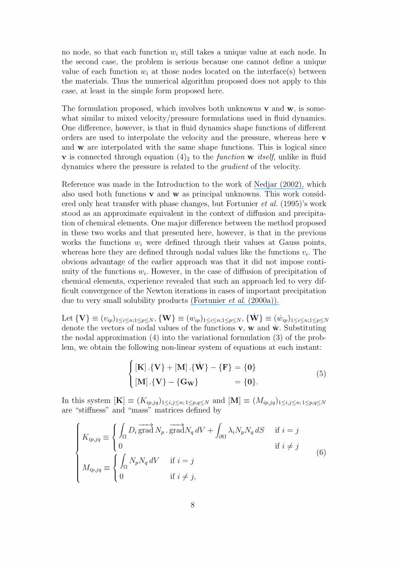
Let V ≡ (vip)1≤i≤n;1≤p≤N , W ≡ (wip)1≤i≤n;1≤p≤N , W ≡ (wip)1≤i≤n;1≤p≤N

denote the vectors of nodal values of the functions v, w and w. Substitutingthe nodal approximation (4) into the variational formulation (3) of the prob-lem, we obtain the following non-linear system of equations at each instant:

[K] .V+ [M] .W − F = 0

[M] .V − GW = 0.(5)

In this system [K] ≡ (Kip,jq)1≤i,j≤n; 1≤p,q≤N and [M] ≡ (Mip,jq)1≤i,j≤n; 1≤p,q≤N

are “stiffness” and “mass” matrices defined by

Kip,jq ≡

∫

ΩDi

−−→gradNp .

−−→gradNq dV +

∫

∂ΩλiNpNq dS if i = j

0 if i 6= j

Mip,jq ≡

∫

ΩNpNq dV if i = j

0 if i 6= j,

(6)

8

and F ≡ (Fip)1≤i≤n; 1≤p≤N and GW ≡ (GW ip)1≤i≤n; 1≤p≤N are vectorsdefined by

Fip ≡∫

∂Ω(J

(p)i + λiv

(p)i )Np dS

GW ip ≡∫

Ωgi(W)Np dV.

(7)

In equation (7)2, gi(w) becomes a function of the vector W since the testfunction w is given by the nodal interpolation (4)2.

It is worth noting that in the term [K] .V of equation (5)1, correspond-

ing to the term∫

Ω Di

−−→grad vi .

−−→grad v∗i dV of equation (3)1, the gradients of the

functions vi are evaluated from these functions themselves rather than fromthe gradients of the functions wi. This is indeed preferable since the func-tions vi are always continuous whereas the functions wi may be discontinuousin some cases. There is a difference here with customary enthalpic methodswhich express the thermal gradient (that is the gradient of v1) in terms ofthe gradient of the enthalpy (that is of w1). This unhappy procedure increasesthe detrimental consequences of the possibly wrong hypothesis of continuityof the functions wi implied by their nodal interpolation.

Following the recommendation of Dalhuijsen and Segal (1986) and Pham(2000), among others, the matrix [M] is lumped in order to eliminate spu-rious oscillations in the time integration of equation (5)1; that is, equation(6)2 is replaced by

Mip,jq =

∫

ΩNp dV if i = j and p = q

0 otherwise.(8)

It has been shown by Ciarlet and Segal (1978) that this lumping has no detri-mental effect on the effectiveness of linear elements (as used in this paper)for problems of diffusion with phase changes. Also, with a small error, thefunction gi in the expression (7)2 of GWip is replaced by its value at node p:

GWip = gi(wp)∫

ΩNp dV (9)

where wp ≡ (wip)1≤i≤n denotes the value of the function w at node p. Withthis simplification, only nodal evaluations of the functions gi(w) are required;no calculations at Gauss points are needed.

2.4 Time discretization

An implicit (backward) Euler algorithm tolerating relatively large time stepsis adopted for the time integration of system (5); this means that the approx-

9

imation

W(t+∆t)

=W(t+∆t) − W(t)

∆t(10)

is made in equation (5)1. System (5), written at time t +∆t, then becomes

RV ≡ [K] .V(t+∆t)+[M]

∆t.W(t+∆t) − F −

[M]

∆t.W(t) = 0

RW ≡ [M] .V(t+∆t) − GW(t +∆t) = 0.

(11)

2.5 Solution procedure

Equations (11) are solved by a Newton-Raphson iterative method. The tangentmatrix to be used in this method is

∂ RV

∂ V(t+∆t)

∂ RV

∂ W(t+∆t)∂ RW

∂ V(t+∆t)

∂ RW

∂ W(t+∆t)

=

[K][M]

∆t

[M] − [L]

. (12)

In this equation [L] ≡ (Lip,jq)1≤i,j≤n; 1≤p,q≤N is the matrix defined (at eachiteration) by

Lip,jq ≡∂GW ip

∂wjq

=

∂gi∂wj

(wp(t+∆t))∫

ΩNp dV if p = q

0 if p 6= q

(13)

where equation (9) has been used. Each iteration thus consists of solving thelinear system

[K][M]

∆t

[M] − [L]

.

δV

δW

= −

RV

RW

(14)

where δV and δW denote the increments of V(t+∆t) and W(t+∆t)looked for.

A further advantage of the lumping of the matrix [M] is that its inversionbecomes straightforward, so that equation (14)2 may easily be solved withrespect to δV:

δV = [M]−1 . ([L] . δW − RW) (15)

so as to eliminate δV in equation (14)1 which thus becomes a system on

10

Fig. 1. Temperature-enthalpy diagram for the Stefan problem

the sole unknown δW:

(

[K] . [M]−1 . [L] +[M]

∆t

)

. δW = [K] . [M]−1 . RW − RV . (16)

3 Application to the Stefan problem

A first test is performed on Stefan’s famous problem of isothermal solidificationof an initially liquid semi-infinite slab. The example considered is identical tothat studied by Fachinotti et al. (1999). The value of the thermal conductivityis 1.08 Wm−1K−1 and Figure 1 shows the temperature-enthalpy diagram. Theapplication of the formalism of Section 2 is straightforward in this case; in-deed the temperature is a well-defined, unambiguous function of the enthalpyalthough the converse is not true. The initial temperature of 0C is identicalto the temperature of transformation.

In this example the derivative dθ/dH of the temperature with respect to theenthalpy per unit volume is strictly zero during the transformation. It hasbeen stressed by Rappaz et al. (1998) that such zero derivatives may generatenumerical difficulties in the Newton-Raphson iterative method used at eachtime-step. This problem is circumvented by using a very small positive valueof 0.10 C/70.26 Jm−3 for the derivative dθ/dH in the small interval 0 ≤ H ≤70.26 Jm−3. This slight modification is introduced only in the left-hand sidematrix [L] of the system (14), not in the right-hand side vector RW, so ithas no effect upon the “exactness” of the numerical solution.

The finite element mesh is composed of two-node linear elements. The element

11

Fig. 2. Temperature distribution at time t = 4 s

Fig. 3. Enthalpy distribution at time t = 4 s

size h is uniform and the time-step ∆t is invariable.

Figures 2 and 3 show the computed temperature and enthalpy distributions attime t = 4 s, together with those corresponding to Carslaw and Jaeger (1959)’sanalytical solution. The value of h is 0.125m and two values of ∆t, 0.2 s and0.5 s, are used. Figure 4 also presents the evolution of temperature in time atx = 1m. The numerical results closely agree with the analytical ones.

In order to more carefully study the accuracy of the numerical solution, let usdefine the error ǫ by the formula

ǫ ≡

√

∫

Ω(θnum − θanal)2 dx . (17)

Figure 5 shows ǫ as a function of h and ∆t. It satisfactorily decreases whenthese parameters go to zero, and is of the same order as in the work ofFachinotti et al. (1999).

12

Fig. 4. Evolution of temperature in time at x = 1m

0.10.2

0.3

00.5

11.5

20

1

2

3

4

5

6

7

8

Element size (m)Time step (s)

Err

or (

°C.m

)

0.5

Fig. 5. Mean quadratic error as a function of element size and time-step

Figure 6 illustrates the efficiency of the Newton-Raphson algorithm. The meannumber of iterations necessary for convergence decreases when the time-stepgoes to zero; two iterations are sufficient for ∆t = 0.05 s.

4 Application to heat transfer in steels with non-instantaneous

metallurgical transformations

4.1 Kinetic and thermodynamic hypotheses

Isothermal phase changes in alloys are often modelled through the follow-ing classical kinetic equation (Johnson and Mehl (1939), Avrami and Mehl

13

Fig. 6. Mean number of iterations necessary for convergence

(1941)):p(t) = 1− exp [−(ft)m] (18)

where p denotes the volume fraction of the product phase, and the “frequency”f and the exponent m material parameters depending on the temperature θ.The origin of time here must correspond to the beginning of the transforma-tion.

In such an integrated form, this equation does not apply to transformationsoccurring during continuous heating or cooling because it includes an influenceof the present temperature but not of the whole thermal history, as is obviouslynecessary. This problem may be solved by differentiating equation (18) withrespect to time and eliminating t between the expressions of p(t) and p(t); onethus get the differential equation

p = mf(1− p)

[

ln

(

1

1− p

)]m−1

m

. (19)

The hypothesis is then made that this equation, which was obtained in thecase of a constant temperature, in fact applies to arbitrary thermal histories.

Even in the “extended” form (19), the kinetic law used is liable to variouscriticisms. It has notably been remarked by Leblond and Devaux (1984) andLeblond et al. (1985) that since p vanishes only if p = 0 or p = 1, equa-tion (19) is incompatible with the general existence, for each temperature, ofan arbitrary “equilibrium” proportion of the product phase reached isother-mally after a very long time. This equation is used here merely for illustrativepurposes; more realistic kinetic laws could equally well be employed, at theexpense of greater complexity.

Once p is known, the specific enthalpy H of the mixture may be obtained from

14

the simple “linear mixture rule”:

H ≡ (1− p)h1(θ) + ph2(θ) (20)

where h1(θ) denotes the specific enthalpy of the parent phase 1 and h2(θ) thatof the product phase 2. Although this expression disregards possible thermo-dynamic interactions between the phases, it is widely considered to providean acceptable approximation of the enthalpy of alloys during phase changes.

Note that in spite of its simplicity, equation (20) implicitly includes the effect ofthe latent heat of the transformation. This is best evidenced by differentiatingit with respect to time:

H =

[

(1− p)dh1

dθ(θ) + p

dh2

dθ(θ)

]

θ + [h2(θ)− h1(θ)] p.

The quantity (1− p) dh1

dθ(θ) + p dh2

dθ(θ) here represents the global specific heat

of the mixture of phases and the quantity h2(θ)−h1(θ) the specific latent heatof the transformation.

4.2 Application of the formalism of Section 2

Equation (20) makes it clear that the specific enthalpy does not only dependon the temperature θ but also on the proportion p of the product phase, whichappears as an extra auxiliary variable. The problems envisaged in Section 2did not include such a variable, so that it is not immediately clear how theformalism developed in this section may be applied to the present case.

In fact this formalism applies to the problem considered here in its time-discretized form. Assume first that an explicit time-discretization is adopted forthe proportion of the product phase; that is, use the approximation p(t+∆t) ≃p(t), or better p(t + ∆t) ≃ p(t) + p(t)∆t. Then p(t + ∆t) is known and nolonger a variable; equation (20) defines H(t+∆t) as an explicit function of thesole variable θ(t + ∆t), θ(t + ∆t) as an implicit function of the sole variableH(t + ∆t), and the equations of the problem do fit into the formalism ofSection 2.

However, explicit approximations of p(t + ∆t) turn out to yield acceptableresults only if very small time-steps are used. “Reasonable” time-steps requirethe use of an implicit scheme for the proportion of the product phase. Such ascheme can be achieved by first using an explicit approximation of p(t +∆t)to evaluate θ(t + ∆t) and H(t + ∆t), but then updating p(t + ∆t) throughintegration of equation (19) between times t and t + ∆t and repeating theprocess up to convergence. In essence, this means using a “fixed-point” al-gorithm to determine the value of p(t + ∆t). An extra difficulty revealed by

15

numerical experience is that p(t+∆t) can be calculated accurately only if θ isitself known accurately between times t and t+∆t, and θ unfortunately variesmuch less smoothly than H and p. The following procedure, which combinesthe advantages of use of an implicit scheme for p and accurate integration ofequation (19), is therefore adopted:

(1) Assume some value of p(t +∆t), for instance p(t +∆t) ≃ p(t) + p(t)∆t,and calculate H(t+∆t) using the formalism of Section 2.

(2) Assume some simple variations of H(t′) and p(t′) on the time-interval[t, t + ∆t] 3 , and solve equation (20) with respect to θ at a number ofintermediary instants in this interval (sub-stepping).

(3) Using the thermal history thus defined, integrate the differential equation(19) to find some new value of p(t +∆t).

(4) Repeat the process up to convergence.

This procedure of solution thus makes use of the formalism of Section 2 ateach iteration.

In the late 1980’s, Rappaz and coworkers introduced “macro-micro” modelsfor the simulation of solidification processes (see for instance Rappaz (1989)’sreview paper). These models essentially consisted of calculating the temper-ature at some “macro” scale by solving the heat diffusion equation, using itto evaluate “micro” variables pertaining to such “micro” phenomena as for-mation of dendrites, microsegregations etc., and finally possibly updating thetemperature using these “micro” variables and repeating the process up toconvergence. There is a striking similarity of principle between such modelsand the numerical procedure proposed here, in which the proportion of theproduct phase plays the role of a “micro” variable in the sense of Rappaz(1989).

4.3 Example

The procedure is illustrated through consideration of an infinite steel plateof thickness 4 mm undergoing an austenite → pearlite transformation duringcooling. The 1D mesh is shown in Figure 7 and consists of 40 linear elementsand 41 nodes. The specific enthalpies of the two phases are provided as func-tions of temperature in Figure 11 below and the value of the thermal conduc-tivity is 20 Wm−1K−1. The value of the exponent m in the kinetic equation(19) is 3.45, and the frequency f is provided as a function of temperature inFigure 8. The initial temperature is 1000C. At the left boundary, at x = 0,the plate exchanges heat with the external medium at a temperature of 20C

3 Equation (10) imposes a linear variation for H(t′), but more refined approxima-tions based on equation (19) are possible for p(t′).

16

through some transfer coefficient of 50 Wm−2K−1. At the right boundary, atx = 4 mm, the plate is insulated.

Fig. 7. Sketch of the thermal problem studied

Fig. 8. Variation of the frequency f (in s−1) versus temperature

Two different time-steps of 10 s and 50 s are employed in order to illustrate thepossible use of relatively large ones. A sub-step of 0.3 s is used to integrate thekinetic equation (19). Less than 10 iterations per time-step reveal necessaryfor correct convergence, even for the larger time-step.

Figures 9 and 10 show the evolutions of the specific enthalpy and the tem-perature in time at x = 1 mm, and Figure 11 shows the specific enthalpyversus temperature at the same position. One can see that the two time-stepsyield almost identical results, in spite of the fact that for the larger one, thetransformation occurs over no more than 2 time-steps. Also, the recalescencephenomenon is very conspicuous in Figures 10 and 11, although it is not inFigure 9.

17

Fig. 9. Evolution of the specific enthalpy in time at x = 1 mm

Fig. 10. Evolution of the temperature in time at x = 1 mm

5 Application to internal oxidation of steels

5.1 Equations of the problem

The application envisaged here involves the diffusion of oxygen and aluminumcoupled with the precipitation of alumina (Al2O3) in a steel matrix. The equa-tions of the problem are recalled briefly here for completeness; more detailscan be found in (Flauder et al. (2005)).

Let CO and CAl denote the mass concentrations of oxygen and aluminum

18

Fig. 11. Specific enthalpy versus temperature at x = 1 mm

atoms in solution in the metallic matrix. Also, let FO and FAl denote the totalmass fractions of oxygen and aluminum, that is including the atoms embeddedin Al2O3 precipitates in addition to those in solution in the matrix. Finally, letPAl2O3

denote the mass fraction of Al2O3 precipitates. Counting the number ofatoms of oxygen and aluminum in all their forms (in solution in the matrix andembedded in precipitates) in some elementary volume 4 , one gets the followingbalance equations:

FO

MO=

CO

MO+ 3

PAl2O3

MAl2O3

FAl

MAl=

CAl

MAl+ 2

PAl2O3

MAl2O3

(21)

where MO and MAl denote the atomic masses of oxygen and aluminum andMAl2O3

the molecular mass of Al2O3.

The equations of diffusion of oxygen and aluminum are obtained by relating (i)the time-derivatives of their total fractions in some elementary volume (whichare unaffected by chemical reactions) to their fluxes through its boundary;and (ii) these fluxes to the gradients of the sole concentrations (since atomsembedded in precipitates do not contribute to diffusion). One thus gets theequations

FO = div(

DO

−−→gradCO

)

˙FAl = div(

DAl

−−→gradCAl

)(22)

where DO and DAl denote the diffusion coefficients of oxygen and aluminum.

4 The “elementary volumes” considered by the macroscopic model employed are infact large enough to contain both the matrix phase and the Al2O3 precipitates.

19

The relation between the total fractions of oxygen and aluminum and theirconcentrations in the matrix is assumed to be governed by local and instan-taneous thermodynamic equilibrium, that is by the law of mass action whichreads

PAl2O3= 0 and C2

AlC3O ≤ KAl2O3

or

PAl2O3> 0 and C2

AlC3O = KAl2O3

(23)

where KAl2O3denotes the solubility product of Al2O3. This law can be re-

expressed as follows using the balance equations (21):

PAl2O3= 0 and

(

FAl − 2 MAl

MAl2O3

PAl2O3

)2 (

FO − 3 MO

MAl2O3

PAl2O3

)3

≤ KAl2O3

or

PAl2O3> 0 and

(

FAl − 2 MAl

MAl2O3

PAl2O3

)2 (

FO − 3 MO

MAl2O3

PAl2O3

)3

= KAl2O3.

(24)For given values of the total fractions of elements FO, FAl, these equations de-fine a complementarity problem on the unknown fraction of precipitate PAl2O3

.This problem has been thoroughly studied (in the general case of n chemicalelements and m precipitate phases) by Leblond (2005), who has shown thatit implicitly defines PAl2O3

, and therefore CO and CAl by equations (21), asunambiguous functions of the pair (FO, FAl).

Finally the boundary conditions consist of prescribing either the flux or theconcentration of each element. It is thus clear that the diffusion and pre-cipitation equations (22) and (23) (with the balance equations (21)), plusthe boundary conditions, fit into the formalism of Section 2, with n ≡ 2,v ≡ (CO, CAl) and w ≡ (FO, FAl).

5.2 1D example

We first consider diffusion and precipitation in a thick, laterally infinite plate.The problem is then 1D in the direction x perpendicular to the surface ofthis plate. The values of the diffusion coefficients of oxygen and aluminum areDO = 8.02 µm2s−1 and DAl = 5.58 10−4 µm2s−1, and that of the solubilityproduct of Al2O3 is KAl2O3

= 2.14 10−18 ppm5. The plate is initially free ofoxygen and the initial total fraction of aluminum (determined by the grade ofthe steel) is 1200 ppm. On the left bounding surface, at x = 0, a fixed oxygenconcentration of 9.24 10−3 ppm is imposed and the flux of aluminum is zero.On the right bounding surface, the fluxes of both oxygen and aluminum arezero. Oxygen gradually penetrates into the plate (inward diffusion) at x = 0,thus inducing precipitation of Al2O3 near the left surface. This precipitation

20

generates an aluminum “sink” which causes aluminum to diffuse toward theleft surface (outwards diffusion).

Figure 12 displays the total mass fraction of aluminum at time t = 60 s, asa function of the distance x from the left surface. Three types of results areshown:

(1) those obtained with the implicit finite element algorithm developed inthis paper, with a time-step of 0.1 s;

(2) those obtained using the explicit 1D finite difference technique of Flauderet al. (2005), with a very small, varying time-step (typically between 10−7

and 10−5 s);(3) those corresponding to the classical analytical solution of Wagner (1959) 5 .

One can see that the agreement with Wagner’s solution is excellent, is spite ofthe numerical difficulty of this example which involves a quasi-discontinuoustotal fraction of aluminum. The agreement between the implicit and explicitnumerical solutions is also excellent, but the computation time is dramaticallyshorter for the implicit calculation (4 s versus 8 min 35 s on a standard 2.13GHz PC with 2 Go memory). Also, less than 5 iterations are sufficient toreach convergence of the Newton iterations at each time-step in the implicitcomputation.

Fig. 12. Distribution of the total mass fraction of aluminum in a thick plate at t=60s5 In theory this solution is for a plate of infinite thickness and a zero solubilityproduct of the precipitate, but it is applicable here because the thickness of theplate is large and the solubility product small.

21

5.3 2D example

We now consider the same problem of inward diffusion of oxygen inducing pre-cipitation of Al2O3 and outward diffusion of aluminum, but now near a squarecorner (2D problem; no analytical solution is available for such a case). Figure13 shows the mesh used and the distribution of the mass concentration ofaluminum at time t = 60 s. Also, Figure 14 shows the distribution of the totalmass fraction of aluminum along the diagonal of the corner (shown in Figure13) at the same instant, for both the implicit calculation (with a time-step of0.01 s) and an explicit one based on a 2D finite element extension of Flauder etal. (2005)’s explicit 1D finite difference technique. The two calculations yieldvery similar results but again, the implicit one requires much less CPU time(2 h 16 min versus 40 h 57 min).

Fig. 13. 2D mesh and iso-contours of the mass concentration of aluminum (in ppm)at time t = 60 s

6 Summary and perspectives

A procedure coupling the finite element technique in space and implicit inte-gration in time has been developed for the numerical simulation of diffusionwith phase changes in solids. This procedure is computationally efficient androbust: it tolerates large time-steps and large nonlinearities, convergence ofthe necessary iterations remaining always quite quick.

22

Fig. 14. Distribution of the total mass fraction of aluminum along the diagonal ofthe corner at time t = 60 s

The advantages brought are particularly clear for the simulation of the si-multaneous and coupled diffusion and precipitation of chemical elements. Thenew algorithm allows to address even numerically difficult cases involving verysmall solubility products of the precipitate phases and nearly discontinuoustotal fractions of elements. Such problems could be dealt with using Flauder etal. (2005)’s technique based on finite differences and explicit time-integration,but only in the 1D case and with very small time-steps implying considerablecomputation times.

In the future, this work will be extended in several directions:

(1) In the case of heat transfer with phase changes, multiple transformationswill be accounted for using the formalism developed by Fortunier et al.(2000b). This is essential for applications to welding for instance.

(2) A convective term will also be added to the heat diffusion equation. Thiswill allow, in those cases involving a moving heat source, to directly lookfor the quasi-steady thermal state in the comoving frame, rather thansimulating the whole thermal history in the fixed frame by a cumbersomestep-by-step method.

(3) In the case of simultaneous diffusion and precipitation of chemical ele-ments, arbitrary numbers of diffusing species and precipitate phases willbe accounted for. This is essential for applications to the majority of re-alistic problems of internal oxidation which involve multiple diffusion (ofoxygen, aluminum, chromium, manganese, titanium, etc.) and precipita-tion of various phases (Al2O3, Cr2O3, MnO, Al2MnO4, etc.).

All of these extensions will require additional, but basically straightforward

23

programming efforts. Indeed they do not imply any basic overhaul of theunderlying theoretical framework.

References

Avrami M. and Mehl R.F. (1941). Kinetics of phase change - Granulation,phase change and microstructure, J. Chem. Phys., 9, 177-184.

Carslaw H. and Jaeger J. (1959). Conduction of Heat in Solids, ClarendonPress, Oxford, UK.

Ciarlet Ph. and Segal A. (1978). The finite element method for elliptic prob-lems, North-Holland, Amsterdam, the Netherlands.

Cetinel H., Toparli M. and Ozsoyeller L. (2000). A finite element based pre-diction of the microstructural evolution of steels subjected to the Tempcoreprocess, Mech. Materials, 32, 339-347.

Comini G., Del Guidice S., Lewis R.W. and Zienkiewicz O.C. (1974). Finite el-ement solution of nonlinear heat conduction problems with special referenceto phase change, Int. J. Numer. Meth. Engng., 8, 613-624.

Dalhuijsen A.J. and Segal A. (1986). Comparison of finite element techniquesfor solidification problems, Int. J. Numer. Meth. Engng., 23, 1807-1829.

Droux J.J. (1991). Three-dimensional numerical simulation of solidificationby an improved explicit scheme, Comput. Meth. Appl. Mech. Engng., 85,57-74.

Eyres N.R., Hartree D.R., Ingham J., Jackson R., Sarjant R.J. and WagstaffJ.B. (1947). The calculation of variable heat flow in solids, Phil. Trans. Roy.Soc. London, 240, 1-57.

Fachinotti V., Cardona A. and Huespe A. (1999). A fast convergent and accu-rate temperature model for phase-change heat conduction, Int. J. Numer.Meth. Engng., 44, 1863-1884.

Flauder P., Huin D. and Leblond J.B. (2005). Numerical simulation of internaloxidation of steels during annealing treatments, Oxid. Metals, 64, 131-167.

Fortunier R., Leblond J.B. and Bergheau J.M. (2000a). Computer simula-tion of thermochemical treatments: modelling diffusion and precipitation inmetals, J. Shanghai Jiaotong Univ., 5, 303-309.

Fortunier R., Leblond J.B. and Bergheau J.M. (2000b). A numerical modelfor multiple phase transformations in steels during thermal processes, J.Shanghai Jiaotong Univ., 5, 213-220.

Fortunier R., Leblond J.B., Pont D. (1995). Recent advances in the numericalsimulation of simultaneous diffusion and precipitation of chemical elementsin steels, in: Phase Transformations During the Thermal/Mechanical Pro-cessing of Steel, Hawbolt and Yue, eds., the Canadian Institute of Mining,Metallurgy and Petroleum, Montreal, Canada, pp. 357-371.

Gremaud P.A. (1991). Analyse numerique de problemes de changements dephase lies a des phenomenes de solidification, Ph.D. thesis, Ecole Polytech-

24

nique Federale de Lausanne, Switzerland (in French).Han H.N., Lee J.K., Kim H.J. and Jin Y.S. (2002). A model for deformation,temperature and phase transformation behavior of steels on run-out tablein hot strip mill, J. Materials Processing Technol., 128, 216-225.

Homberg D. (1996). A numerical simulation of the Jominy end-quench test,Acta. Mater., 44, 4375-4385.

Johnson W.A. and Mehl R.F. (1939). Reaction kinetics in process of nucleationand growth, Trans. AIME, 135, 416-458.

Leblond J.B. (2005). Mathematical results for a model of diffusion and precita-tion of chemical elements in solid matrices, Nonlinear Anal. B: Real WorldApplic., 6, 297-322.

Leblond J.B. and Devaux J. (1984). A new kinetic model for anisothermalmetallurgical transformations in steels including effect of austenite grainsize, Acta Metall., 32, 137-146.

Leblond J.B., Mottet G., Devaux J. and Devaux J.C. (1985). Mathematicalmodels of anisothermal transformations in steels, and predicted plastic be-haviour, Materials Sci. Technol., 1, 815-822.

Lewis R. and Roberts P. (1987). Finite element simulation of solidificationproblems, Appl. Sci. Res., 44, 61-92.

Morgan K., Lewis R.W. and Zienkiewicz O.C. (1978). An improved algorithmfor heat conduction problems with phase change, Int. J. Numer. Meth. En-gng., 12, 1191-1195.

Mundim M.J. and Fortes M. (1989). Evaluation of finite element methodutilised in the solution of solid-liquid phase change problems, in: NumericalMethods in Thermal Problems, Lewis and Morgan, eds., Pineridge Press,Swansea, UK, vol. 6, pp. 90-100.

Murthy Y., Venkata Rao G. and Krichna Iyer P. (1996). Numerical simulationof welding and quenching processes using transient thermal and thermo-elasto-plastic formulations, Comput. Structures, 64, 131-154.

Nedjar B. (2002). An enthalpy-based finite element method for nonlinear heatproblems involving phase change, Comput. Structures, 80, 9-21.

Pham Q.T. (1985). A fast, unconditionally stable finite difference scheme forheat conduction with phase change, Int. J. Heat Mass Transfer, 28, 2079-2084.

Pham Q.T. (2000). Comparison of general-purpose finite element methods forthe Stefan problem, Numer. Heat Transfer B: Fundamentals, 27, 417-435.

Rappaz M. (1989). Modelling of microstructure formation in solidification pro-cesses, Int. Materials Rev., 34, 93-123.

Rappaz M., Bellet M. and Deville M. (1998). Traite des materiaux n10 :Modelisation en science et genie des materiaux, Presses Polytechniques etUniversitaires Romandes, Lausanne, Switzerland (in French).

Rolph W.D. and Bathe K.J. (1982). An efficient algorithm for analysis ofnonlinear heat transfer with phase changes, Int. J. Numer. Meth. Engng.,18, 119-134.

Serajzadeh S. (2004). Modelling of temperature history and phase transforma-

25

tions during cooling of steel, J. Materials Processing Technol., 146, 311-317.Voller V.R. (1996). An overview of numerical methods for phase change prob-lems, Adv. Numer. Heat Transfer, 1, 341-375.

Wagner C. (1959). Reaktionstypen bei der oxydation von Legierungen,Zeitschrift fur Elektrochemie, 63, 772-782.

26