An impact assessment of electricity and emission allowances pricing in optimised expansion planning...

Applied Energy 88 (2011) 3791–3806

Contents lists available at ScienceDirect

Applied Energy

journal homepage: www.elsevier .com/locate /apenergy

An impact assessment of electricity and emission allowances pricingin optimised expansion planning of power sector portfolios

Athanasios I. Tolis ⇑, Athanasios A. RentizelasIndustrial Engineering Laboratory, Mechanical Engineering School, National Technical University of Athens, Zografou, 15780 Athens, Greece

a r t i c l e i n f o

Article history:Received 7 December 2010Received in revised form 23 February 2011Accepted 28 April 2011Available online 19 May 2011

Keywords:Electricity pricesPower sector portfolioOptimisationOperational researchEmissions trading

0306-2619/$ - see front matter � 2011 Elsevier Ltd. Adoi:10.1016/j.apenergy.2011.04.054

⇑ Corresponding author. Tel.: +30 210 7722385; faxE-mail address: [email protected] (A.I. Tolis).

a b s t r a c t

The present work concerns a systematic investigation of power sector portfolios through discrete scenar-ios of electricity and CO2 allowance prices. The analysis is performed for different prices, from regulatedto completely deregulated markets, thus representing different electricity market policies. The modellingapproach is based on a stochastic programming algorithm without recourse, used for the optimisation ofpower sector economics under multiple uncertainties. A sequential quadratic programming routine isapplied for the entire investigation period whilst the time-dependent objective function is subject to var-ious social and production constraints, usually confronted in power sectors. The analysis indicated theoptimal capacity additions that should be annually ordered from each competitive technology in orderto substantially improve both the economy and the sustainability of the system. It is confirmed thathigher electricity prices lead to higher financial yields of power production, irrespective of the CO2 allow-ance price level. Moreover, by following the proposed licensing planning, a medium-term reduction ofCO2 emissions per MW h by 30% might be possible. Interestingly, the combination of electricity pricessubsidisation with high CO2 allowance prices may provide favourable conditions for investors willingto engage on renewable energy markets.

� 2011 Elsevier Ltd. All rights reserved.

1. Introduction

Optimal expansion planning of electricity production has beenan important goal for grid designers, energy policy makers, opera-tional researchers and economic analysts. The incomes from elec-tricity selling to the grid, as well as the power production costs,both determine the economics of the power sector, though to adifferent extent. The compensation of the electricity producersdepends on the System Marginal Prices (SMP), which areannounced by the grid operators based on the market dynamics.On the other hand, the costs of power production may dependon the installation of mature but proven workhorse technologiesor, on the displacement of obsolete plants by emerging eco-friendly technologies necessitated by the recent environmentaldirectives. The fuel costs and the power loads demanded by theend-users may additionally impact the aggregate power produc-tion costs. Moreover, the economics of the power sector dependon the current generation mix thus leading to initiatives relatedwith its expansion planning. Such initiatives may include deregu-lated pricing policies as well as the determination of capacityshares from each competing technology.

ll rights reserved.

: +30 210 772 3571.

Electricity production planning may be influenced by interven-tions on licensing policies, fiscal conditions and price volatility. Theevaluation of policies used for the assistance of project designersusually requires the discounting of future incomes and expenses.The Discounted Cash Flow (DCF) method has been extensively usedin past energy investment studies. These were characterised byincorporating arbitrary values of risk premium in the interest rates,which were assumed to remain constant throughout the projects’operational life time. In practice, high values of interest rate wereused and moreover, immediate investments were considered.

Modern business plans have focused on time-varying methodsand therefore, previously irreversible investment decisions areprogressively replaced by flexible planning, subject to optimisationprocesses. Thus, the minimisation of production costs and thedetermination of the optimal generation mix may be inquired overtime. Significant contributions on power sector portfolio analysisand optimisation have been recently available, focusing on non-probabilistic or probabilistic models [1,2] for the representationof multiple uncertainties, usually confronted in energy investmentanalysis, expansion planning and the related CO2 mitigationstrategies.

With these advances on hand, the analysis of energy invest-ments may now utilise powerful computational tools applicablefor many case studies. The present article addresses the case ofthe Greek Power Sector. The capacity additions – recently installed

http://dx.doi.org/10.1016/j.apenergy.2011.04.054

mailto:[email protected]

http://dx.doi.org/10.1016/j.apenergy.2011.04.054

http://www.sciencedirect.com/science/journal/03062619

http://www.elsevier.com/locate/apenergy

Nomenclature

At generic notation for stochastic variables evolvingaccording to a GBM model

aa,i availability factor for plant (i) (%)ac,i capacity factor for plant (i) (%)b(i) learning rate of plant (i) constructionCfi,z fuel cost during year (z) for plant (i) (€/MW hel)Ci;v capacity installed in the past (year v before the initiation

of the investigated time-period) for plants (i) and whoseoperational life time has ended (MW)

Ci,v capacity installed in the past (year v before the initiationof the investigated time-period) for plants (i) (MW)

Cvi,z fixed (Operational and Maintenance) cost of electricityproduction for plant (i) in year (z) (€/MW)

D diffusion vector function (–)dWt Wiener (Brownian Motion) vector differential, normally

distributed: � eN (0, 1)Dz discounting factor of year zdz,a aggregate electricity demand for year (z) (actual data in

MW hel)dz,f aggregate electricity demand for year (z) (simulated

projection in MW hel)ECO2i emissions generated by using a specific technology (i)

(tons CO2 equivalent)Eni the annual maximum potential of natural resources for

technology (i) (MW)fCO2i CO2 emission rate of fuel type (i) (tons CO2 equivalent/

MW h)I number of electricity production technologiesIi,v investment cost for orders of plant type (i) made in year

(v) (€/MW)

Li,z installed capacity during year (z) for plant category (i)(MW)

mr power reserve marginni power production efficiency for plant (i) (%)NPV Net Present Value of a project (€)Pcz projected peak power demandpCO2z price of CO2 allowances for the year (z) (€/tons CO2

equivalent)pez forward electricity price for year (z) (selling to the grid

in €/MW h)Pi,z aggregate electricity energy production during year (z)

for plants (i) (MW hel)RE number of electricity production technologies based on

renewable energy sourcesrin inflation rate (%)rt interest rate (%)Tli construction, setup and commissioning time of plant

type (i) (years)Toi operational life-time for each plant type (i) (years)V volatility vector function (–)v counter of the years of investment decisions (capacity

orders)Xi,v orders made in year (v) for plant (i) (MW)Xi;v capacities ordered in year (v) for plant (i) and whose

operational life time has ended (MW)Y the entire studied time-period (years)z counter of the years of plants operationhi,z plant load factor (operation intensity) during year (z) for

plant (i) (%)l mean drift function (–)

3792 A.I. Tolis, A.A. Rentizelas / Applied Energy 88 (2011) 3791–3806

and connected to the national grid – have been questioned for theirenvironmental implications and financial performance, especiallywhen considered in the context of the EU emissions trading system(EU-ETS), which has set the rules of the emissions’ trading market.On the other hand, the power demand is marginally served in peakseasons (e.g. in temperature extremum) thus stressing the underly-ing grid commitment issues. Moreover, the Greek Power Sector hasbeen criticised for not complying with the emission constraints, setfor its power generation mix. Therefore, an urgent need hasemerged for a thorough analysis of the Greek power portfolio aim-ing at the minimisation of the aggregate production cost, whilstkeeping the power supply failures (system black-outs) to a mini-mum and complying with the European environmental constraints.This type of analysis may also contribute to the identification ofinvestment opportunities based on emerging technologies. Attrac-tive projects might then be realised, given that an admissible mod-elling of electricity and emission allowance pricing is available.

The objective of the research is the assessment of the impact ofelectricity and CO2 allowance prices to the future structure of theGreek Power Sector. The ultimate goal is the determination of theoptimal generation mix which is inquired on an annual basis in or-der to set the power licensing policy for the oncoming 25 years.Four different electricity price scenarios are investigated: (a) Pricesregulated and evolving according to stochastic inflation rates, (b)deregulated and simulated through random walk process basedon historical data, (c) semi-regulated to the extend that the pricesfor conventional producers are deregulated and stochasticallyevolving according to historical data, whilst the prices for renew-able energy producers are fixed and evolving according to stochas-tically evolving inflation rates and (d) semi-regulated to the extendthat the prices for conventional producers are deregulated and sto-chastically evolving according to historical data, whilst the prices

for renewable energy producers are fixed and follow the drift ofthe conventional prices. Furthermore, two scenarios of CO2 allow-ance prices evolution are assumed thus dealing with the uncertainbehaviour of emissions trading markets: (I) The allowance pricesregress around their current levels by following a random walk pro-cess and (II) the allowance prices revert to a long-run mean of 31Euros/tn CO2. The above eight scenarios (A, B, C, D) – (I, II) may beinteresting for policy makers willing to provide optimal electricityproduction in terms of system economics and anticipated CO2 emis-sions, whilst meeting the power demand targets and complyingwith the imposed market and environmental constraints.

Apart from the analysed pricing impact in optimised expansionplanning, the contribution of the present study also lies on thenon-linear stochastic programming approach, the utilised con-straints as well as on the statistical analysis of the results. The abovewill be analysed in detail in the next sections, which are essentiallystructured as follows: In Section 2, the related recent studies are pre-sented. In Section 3 a description of the case study is given and themathematical modelling of the problem is formulated. The technicaldetails of the numerical algorithm and the input data are describedin Section 4. Section 5 includes the results of the numerical experi-ments conducted, with critical comments on the relevant graphicalrepresentations. A statistical error analysis of the results is per-formed in Section 6 to validate the model’s reliability. Finally, in Sec-tion 7 the concluding remarks of the research are summarised.

2. Background

2.1. Power portfolios, electricity pricing impact and risk analysis

Bar-Lev and Katz [3] introduced the mean variance portfolioanalysis in fossil fueled power sector. More recent research [4–6]

A.I. Tolis, A.A. Rentizelas / Applied Energy 88 (2011) 3791–3806 3793

extended the analysis to various power expansion mixes. Focus onmean–variance portfolios has been shown in some applicationstesting different risk measures [7,8]. Mean–variance frameworkshave been proposed to address the energy portfolio planning andthe optimal allocation of positions in peak and off-peak forwardprice contracts [9]. It has been shown that optimal allocationsare based on the risk premium differences per unit of day-aheadrisk as a measure of relative costs of hedging risk in the day-aheadmarkets. The influence of the risk management has been also ana-lysed in further studies concerning either solely electricity produc-tion or multi-objective functions comprising of combined heat andpower production [10,11]. Multiple objectives have been also ad-dressed in some case studies of discrete regional power portfoliosunder demand uncertainty [12,13]. In [13] the multi-objectivefunction was extended by assigning cost penalties to non-costattributes to force the optimisation to satisfy non-cost criteria,whilst still complying with environmental and demand con-straints. The impacts of uncertain energy prices on the supplystructures and their interaction with the demand sectors havebeen analysed in the work of Krey et al. [14]. Decision support toolshave been developed [15] seeking for globally optimal solutions,taking into account financial and economical conditions and con-straints imposed at an international level.

The analysis of individual power-plant strategies (i.e. [16–18])as well as the optimisation of power expansion planning (i.e.[19–21]) might be separated in two discrete research categories.The present study might be classified in the latter category inwhich the optimal structure of power generation may be inquired,though considering individual investment opportunities in abroader sense: Suboptimal generation mixes imply that individualplants might sometimes operate under imperfect financial condi-tions. On the contrary, compliance with optimal investment timingmight lead to optimal system NPV thus allowing significant profitchances for individual players. The optimisation of energy portfo-lios relies on the determination of the objective function represent-ing the aggregate Net Present Value (NPV) of the system (powersector). This function has to be optimised whilst being subject toan appropriate set of constraints. The resulting optimal pointdetermines the power generation mix for which the aggregate sys-tem NPV is maximised, thus indicating the optimal investing timeas well as the upper bound share of capacities from each technol-ogy, allowed to be ordered in a specific time point.

The optimisation of the power generation mix may entail com-plicated algorithms for handling the non-linear functional relation-ships of multi-variable sets and constraints. Multiple uncertaintiesmay be introduced as inputs, whilst the Lagrangian functions usu-ally become discontinuous due to various conditional algorithmicstatements, thus inhibiting smooth, global results. Reliable trust-region algorithms have been recently available [22,23] thus allow-ing more accurate results within acceptable computational times.They are widely used in operational research applications, butthe competing Sequential Quadratic Programming (SQP) solversmay outperform them both in terms of accuracy and reliability.SQP routines are based on the solution of the Karush–Kuhn–Tucker(KKT) equations [24] which are comprised of a combined Lagrang-ian formulation of the objective function and the constraints set.The SQP solvers are used in order to approximate the KKT equa-tions with a convex quadratic formulation, thus ensuring continu-ity. Moreover, convexity constitutes both necessary and sufficientcondition for the KKT equations to be resolved thus leading toglobal optimisation of the quadratic approximation. An overviewof the KKT equations and details of the computational SQP solversmay be found in Fletcher [25] or Biggs and Hernandez [26], butthey are also outlined here in Appendix A.

In the present research, a non-linear SQP routine is embeddedin a stochastic programming algorithm without recourse. This

method leads to a single strategy for the entire time horizon, oper-ating on the average of all the stochastic input future states. Thestochastic programming approach has been effectively used in pastand recent researches of power generation planning under uncer-tainty [13,21,27,28]. The research analysed in [13] in particular,comprises of a stochastic programming algorithm with recourse,thus embedding the uncertainties’ modelling in the optimisationiterations. Nonetheless, linear solvers were mainly used in theabove studies, instead of the non-linear SQP solver implementedin the present research. Moreover, different objective functionsand constraints are used here, approaching the environmental lim-itations, the emissions trading system, as well as the stability andthe reliability of the grid.

2.2. Time dependent investments under uncertainty

The analysis of power sector portfolios under multiple uncer-tainties may depend on the evolution of various stochastic vari-ables, which determine the efficiency of energy investmentopportunities. Various computational algorithms have been re-cently applied for the representation of stochastically evolvingvariables. The autoregressive models [29] are mainly used for thesimulation of stationary and non-stationary time-series, whilstthe random-walk algorithms [30], including Ito and Ornstein–Uhlenbeck processes, may be considered as particular cases ofautoregressive models when dealing with discrete time. In compu-tational practice, the above two processes are applied through theGeometric Brownian Motion (GBM) and the mean reverting (MR)models respectively. The Cox–Ingersoll–Ross (CIR) and the Vasicekmodels [31–33] are mean-reverting derivatives mainly used for theprediction of interest and inflation rates. The accuracy and thecomputational cost of the above mentioned random-walk algo-rithms may depend on the utilised solvers which are basicallycomprised of Euler–Marujama routines [34,35]. Moreover, theymay depend on the number of a Monte-Carlo solver trials [36] usedto average the multiple lognormal solutions set.

Among the stochastic variables commonly seen in the analysisof energy investments, the electricity prices, the fuel and the CO2

allowance prices as well as the energy demand, represent the mostsignificant business, and/or climatic uncertainties [17,37–41]. GBMand MR models have been recently applied for the representationof the evolution of stochastic electricity prices [17,21,42]. The dis-counting factor and more specifically the interest rates may intro-duce additional uncertainties in the model. Ingersoll and Ross [33]and Tolis et al. [43] suggest that the interest rate volatility may bean important factor for the investment decision. In the review ofDias and Shackleton [44] switching between the options to investor disinvest is analysed considering different methods of stochasti-cally evolving interest rates: the (CIR) model and the Vasicek mod-el. In more recent studies [45] it is argued that the simulation ofinterest rates may contribute to the elimination of arbitrary riskpremium assumptions, mainly within the framework of real-options models. The capital costs may decrease over time due tothe global experience on similar projects, introducing furthertime-dependent characteristics in the analysis of energy invest-ments [21,46,47].

3. Modelling approach

3.1. Uncertainties modelling and assumptions

In the present research, forward contracts have been consideredfor the prices of electricity selling to the grid. Forward prices maynot contain information about the very short term variations of theunderlying spot prices as the latter are averaged over discrete time


intervals [48]. Both spot and forward prices are characterised bynormally distributed variations (noise) as observed in the raw datasets retrieved by the Greek System Operator [49]. Based on the factthat the GBM and the MR processes require normally distributedBrownian differentials, it is assumed that:

A. The evolution of forward prices is represented through ran-dom walk processes (GBM/MR).

GBM and MR models have been adopted in several past re-searches for the representation of the evolution of forward electric-ity prices, thus considering the absorption of jumps and spikeprocesses over time [16,50,51]. Either endogenous [17] or exoge-nous [21,42] modelling of the evolution of spot electricity pricesthrough GBM or MR processes have been adopted in past studies,indicating a wide range of applications. It has been shown thatthe impact of investors’ actions on electricity prices is minimised[48,52] when multiple investors are considered, provided thatthe following two assumptions are additionally made:

B. Market equilibrium is considered.C. The investors’ profit is a direct function of electricity prices.

In the present work the above assumptions have been alsoadopted and therefore, the effect of multiple investors’ actions onthe evolution of forward prices has been considered to be minimal.However, the dynamics of the electricity prices evolution mayadditionally depend on the evolution of the remaining stochasticcommodities for which uncertainty may be introduced: fuel andCO2 allowance prices, electricity demand as well as interest andinflation rates. For this reason, a correlation of all the participatingBrownian differentials has been performed, thus permitting someform of endogenous modelling of the uncertainties. The requiredstatistical factors of data correlation have been extracted fromthe historical data of the stochastic variables whilst a similar pro-cedure has been followed for the mean drift and the volatilityparameters as in Clewlow and Strickland [53].

The evolution of the stochastic variables is based on the numer-ical solution of the corresponding Stochastic Differential Equations(SDE). GBM models are used when the past data fail to converge toa long run mean, whilst MR models are used in the opposite case.The evolution of the interest rates is represented through a CIRmodel, which is an MR derivative, suitable for producing non-neg-ative forecasts, as required in real world interest rates. The entireMonte-Carlo approximation of the underlying uncertainties iscomprised of the following two steps: (a) producing multiple SDEsolutions using an Euler–Marujama solver and (b) averaging themultiple solution sets; the average path of each variable is furtherintroduced as input in the optimisation algorithm. The above pro-cess precedes the optimisation algorithm, thus allowing the reduc-tion of the floating point operations during its iterative numericalprocesses. Alternatively, one may run the optimisation code foreach one of the multiple input combinations of SDE paths, requir-ing an excessive number of complete optimisation cycles. How-ever, this option, namely a stochastic programming algorithmwith recourse [13,42] has not been the approach of the presentwork. Various reasons like the numerous variables, comprising oflong-term investment horizon (>40 years) for various technologies,as well as numerous non-linear constraints, promoted the decisionfor the final simplified approach, namely a stochastic programmingalgorithm without recourse.

3.2. An overview of the case study

The Greek Power Sector is the market under uncertainty forwhich an optimal structure is sought, in terms of energy produc-

tion and fuel sources. A variety of technologies are examined toform the optimal portfolio. Existing base-load technologies (mainlyfossil fuelled) and competing emerging technologies (mainly basedon renewable sources) are considered as potential contributors tothe power generation mix. The objective function is comprised ofthe aggregate benefit from electricity selling to the grid, subjectto environmental constraints and State regulations. The stabilityof the grid, the total power demand, and the availability of energysources are additional targets to be met. Four different scenariosare investigated in order to assess the impact of electricity pricesevolution:

(a) electricity prices regulated: evolving according to inflationrates,

(b) electricity prices deregulated: forecasted according to a sto-chastic procedure and based on historical data,

(c) electricity prices semi-regulated: prices of conventional pro-ducers are deregulated and stochastically evolving accordingto past data, whilst the prices for renewable energy produc-ers are contractually fixed and evolving according to infla-tion rates

(d) electricity prices semi-regulated: prices of conventional pro-ducers are deregulated and stochastically evolving accordingto past data, whilst the prices for renewable energy produc-ers are contractually fixed and follow the drift of the conven-tional forward prices.

The above electricity prices are further processed in order toform the forward prices evolution paths, required for the optimisa-tion model. Apart from the electricity price uncertainty, a non-sta-tionary behaviour has been modelled for the CO2 allowance prices,by assuming two discrete scenarios:

(I) CO2 allowance prices regress around their recent observa-tions slightly increased in the long term,

(II) CO2 allowance prices regress around a higher long run mean(31 Euros/tn CO2) with a moderate mean-reverting speed.

3.3. Mathematical formulation

The context of the study is the existing power sector, in whichthe prices of electricity, fuel and CO2 allowances as well as theinflation rates are assumed to evolve through random walk(GBM) processes, as formulated by the following Eq. (1):

dAt ¼ lðtÞ � Atdt þ Dðt;AtÞ � VðtÞdWt ð1Þ

where by At, the above mentioned stochastic variables are denotedusing a generic notation. The evolution of the risk-free interest ratesis represented through the Cox–Ingersoll–Ross (CIR) model (Eq. (2)),resulting to non-negative forecasts. This is ensured by the compo-nent (r1=2

t ) which is included in the diffusion vector function (D):

drt ¼ lðtÞ � ½LðtÞ � rt �dt þ Dðt; r1=2t Þ � VðtÞdWt ð2Þ

The use of stochastic interest rates contributes to the endoge-nous modelling of the multi-variate problem by avoiding arbitraryassumptions and this may have direct implications on the financialresults, as explained in [43]. Investing in the electricity market mayincorporate some risk. An approximation of the risk uncertaintymay be derived from the combined simulations of the underlyingfiscal uncertainties, thus reflecting the difference between a sto-chastic NPV calculation (with optimised investment entry times)and a traditional DCF calculation. In the present study, the dis-counting factor Dz is calculated using the above non-constant,risk-free interest rates (Eq. (2)) and a discrete discountingformulation:


Dz ¼Yz

t¼1

ð1þ rtÞ�1 ð3Þ

The independent variables of the optimisation problem arecomprised of the capacities ordered in the year v (Xi,v in MW)and the load factor hi,z of the operational power plants during yearz (z – v), for power plants of technology i. hi,z is a dimensionlessfactor representing the usage intensity of power plants, i.e., the ac-tual operating time over the annually available time.

A detailed modelling of the capacities installed in different timespots is further required. Thus, the capacity additions (either or-dered in the past or planned for the future) may be linked withthe currently installed capacity (Li,z in MWel) using the followingformulation:

Li;z ¼Xz�Tli

v¼1

Xi;v þX0

v¼�40

Ci;v �Xz

v¼1

Xi;v �X0

v¼�40

Ci;v 8i 0 6 z 6 Y ð4Þ

where:

Xi;v ¼ 0 v þ Tli 6 z 6 v þ Tli þ Toi

Xi;v ¼ Xi;v v þ Tli þ Toi 6 z

Ci;v ¼ 0 v þ Tli 6 z 6 v þ Tli þ Toi

Ci;v ¼ Ci;v v þ Tli þ Toi 6 z

The dashed symbols denote the capacity additions that have al-ready exceeded their operational life time. With the above rela-tionship it is ensured that the plants exceeding their operationallife-time, may not contribute anymore to the power productionprocess. The electricity energy production Pi,z (Pi,z in MW hel) repre-sents the aggregate energy produced by the operational powerplants of type (i) during year z:

Pi;z ¼ Li;zhi;zaa;iac;i � 8760 8i; z ð5Þ

This is further used in the discrete optimisation as a factor of theincomes and the expenses contributors. The objective function rep-resents the NPV of the system and includes the aggregate incomes(electricity selling and emissions trading) and expenses (fixedcosts, variable costs, emission allowances, investment costs, etc.)in present values. Its mathematical formulation may be repre-sented by the following equation:

NPVðXi¼1;v :; . . . ;Xi¼I;v ; hi¼1;z:; . . . ; hi¼I;zÞ ¼max

PI

i¼1

PYz¼1

pezDzPi;z �PI

i¼1

PYz¼1

Cfi;zDzPi;z �PI

i¼1

PYz¼1

Cv i;zDzLi;z �PYv¼0

PI

i¼1Ii;vXi;v

�PI�RE

i¼1

PYz¼1

Pi;z �fCO2i

ni� Dz � pCO2z

þPRE

i¼1

PYz¼1

Pi;z �PI�RE

i¼1ECO2iPI�RE

i¼1Pi;z

� Dz � pCO2z

8>>><>>>:

9>>>=>>>; ð6Þ

where the factor Dz is calculated using Eq. (3). A more detailedexpression of Eq. (6) can be seen in Appendix A (Eq. (A5)) whereall the different contributors of the NPV function are analyticallyexpressed in relationship with the requested capacity orders. Onemay notice that the maximisation of the aggregate system NPV isrequired instead of the minimisation of the aggregate power pro-duction cost, thus allowing the estimation of the anticipated profitsor losses.

Concerning the energy produced in excess to the demand, it isnoted that this condition may occasionally occur during thenumerical iterations of the optimisation algorithm until it con-verges to an optimal solution. In the present research, any exces-sive energy produced is assumed to have zero (income) value, asit cannot be exploited by the system. On the other hand, the pro-duction costs of the non-served energy, contribute (being a partof the expenses) in the NPV objective function and therefore they

are always calculated (Eq. (6)). As a result, the optimisation algo-rithm tends to eliminate any excess energy production, by itera-tively attempting to reduce the overall system costs.

The last two terms in Eq. (6) represent the emissions tradingcosts and revenues respectively. The expenses of the required emis-sion allowances for conventional power plants are represented bythe left term with the (�) sign. The revenues are represented bythe right term with the (+) sign and correspond to the incomes fromtrading the emission allowances generated by using renewable en-ergy sources. They result from the multiplication of the renewableenergy generated with the emissions factor of the current conven-tional generating mix and the allowance prices. The emissions fac-tor of the current conventional mix, denoted by the fractional termPI�RE

i¼1ECO2iPI�RE

i¼1Pi;z

, implies the assumption that the renewable energy gener-

ated, replaces energy that would otherwise be produced by the con-ventional generation mix of technologies of the country.

The fixed costs as well as the logistical fuel costs (only for thosefuels with no available historical data) are approximated by com-pounding their present values in the future using the stochastically(GBM) evolving inflation rate:

Cfi;z ¼Yz

t¼1

ð1þ rin;tÞ" #

� Cfi;0 8i ð7Þ

Cv i;z ¼Yz

t¼1

ð1þ rin;tÞ" #

� Cv i;0 8i ð8Þ

In this study the past capacity additions of the last 40 years aretaken into account due to unavailability of older data. The unitaryinvestment costs Ii,v, of a power plant type (i) ordered in the year(v) depend on the technical advances arising from long periods ofcumulative experience on construction of such power productionunits in the domestic market. This can be mathematically formu-lated as follows:

Ii;v ¼ Ii;0 �Pv

k¼1Xi;k þP0

v¼�40Ci;vP0v¼�40Ci;v

" #log2 ½1�bðiÞ �

8i ð9Þ

The capital costs of the year 2009 are used as a reference value(Ii,0) for each technology (i).

The objective NPV function of Eq. (6) is subject to the followingconstraints:

(1) Non-negativity constraints
The factor (hi,z) may take values in the range: 0 6 hi;z 6 1 (hi,z = 0means a non-operational power plant whilst hi,z = 1 implies themaximum operational time in the year z). Moreover, the annualcapacity orders for new power plants Xi,v should be positivenumbers: Xi,v > 0, "i, v.
(2) Natural resource availability
The plants from each technology may not produce more cumu-lative power than the maximum energetic potential of the cor-responding natural resources, domestically available:
Li;z 6 Eni 8i; z ð10Þ


where the aggregate installed capacity of technology (i) (Li,z) is cal-culated using Eq. (4).

(3) Demand constraintsMeeting the demand target is a basic condition ensuring socialacceptance of power production at a national level. The ratio-nale for this constraint was based on the assumption that a pos-sible generic failure of power supply (system black-out) wouldresult to an excessive social cost. This case should be avoided inthe expense of additional capacity orders causing a system NPVreduction. Therefore the average annual electricity energy pro-duction is assumed to be at least as much as the simulatedannual electricity energy demand projection. This constraintcan be mathematically formulated as follows:

XI

i¼1

Pi;z P dz;f )z}|{ð4Þ;ð5ÞXI

i¼1

Xz�Tli

v¼1

Xi;v þX0

v¼�40

Ci;v �Xz

v¼1

Xi;v �X0

v¼�40

Ci;v

!

� hi;zaa;iac;i � 8760 P dz;f 8z ð11aÞAn additional reliability requirement may be imposed by statingthat the installed capacities should be able to serve the peakpower demand. In that case the availability and the intensity fac-tors have been considered to be equal to 1, meaning full-loadoperating conditions with guaranteed fuel availability. However,this may not be the case for the wind turbines and the photovol-taic (PV) plants as they certainly depend on meteorological con-ditions, which are unpredictable in the medium term. Based onpast observations, the peak-power spots generally follow a lineartrend and therefore have been linearly projected to the future.An additional safety factor has been further multiplied to theprojected peak-power demand in order to account for the possi-bility of some plants’ failure or fuel unavailability [13,21]. Themathematical formulation of this constraint is represented inEq. (11b):XI

i¼1

aa;i � Li;z P Pcz � ð1þmrÞ½8z; aa;i ¼ 1;

8i except wind farms and PVs for which aa;i 6 1� )z}|{ð4Þ

�XI

i¼1

aa;i �Xz�Tli

v¼1

Xi;v þX0

v¼�40

Ci;v �Xz

v¼1

Xi;v �X0

v¼�40

Ci;v

!P Pcz � ð1þmrÞ ð11bÞ

The above two-fold demand constraints (11a) and (11b) mightbe able to model any possible case of the system’s reliability limits(either total energy or peak power) depending on which constraintproves to be stricter.

(4) Grid stability
Some power generation technologies, which strongly dependon weather conditions, might constitute a base-load solutionin the long term (i.e. photovoltaic and/or wind farms). How-ever, despite their certain advantages (short setup periods, zeroemissions, zero fuel requirements) they often suffer fromunavailability of natural resources. These – occasionally unpre-dictable – conditions might impact the stability of the nationalgrid and the reliability of power supply. Also, despite the factthat there is no consensus on the maximum allowable percent-age of renewable energy sources to secure the grid stability,scientists agree that there is currently an upper limit on renew-able power infusion to the grid [54]. For this reason a con-straint is imposed ensuring that the total energy productionfrom these specific types may not exceed 50% of the total en-ergy demand:
XRE

i¼1

Pi;z 6 0:5 � dz;f 8z ð12Þ

(5) Environmental constraintsThese are obligatory constraints applied in every country partic-ipating in the Kyoto Protocol. Greece is required to meet the fol-lowing targets imposed by the EU directive 2001/77/EC [55]:

(5a) The renewable energy technologies should obtain a share ofmore than 20.1% of the total domestic electricity productionby the year 2010. Hence:

XRE

i¼1

Pi;z > ð0:201Þ �XI

i¼1

Pi;z 8z P 2010 ð13Þ

(5b) The renewable energy technologies should obtain a share ofmore than 30% of the total domestic electricity productionby the year 2020. Hence:

XRE

i¼1

Pi;z > ð0:3Þ �XI

i¼1

Pi;z 8z P 2020 ð14Þ

4. The numerical algorithm

4.1. Inputs of the model

The numerical algorithm used for the determination of the opti-mal power generation mix comprises of the following discretesteps: (a) Retrieving technological and economical inputs, (b)retrieving historical time-series of stochastic variables, (c) simulat-ing the evolution of stochastic variables and (d) optimisationroutine. The inputs used in the present study are shown in Table 1.

The historical data of the stochastically fluctuating variableshave been acquired by various sources. The past demand loadsand SMPs have been acquired by the national grid operator [49].The historical data of fuel prices have been provided by the GreekState [56] the Statistical Service [57], the natural gas provider [58]and the International Energy Agency [59]. The recent CO2 allow-ance prices were retrieved from Point-Carbon [60]. For the caseof biomass, lacking price historical data, their current gate feeswere estimated using a holistic Activity Based Costing procedure[61]. After the current supply chain costs are estimated, they arepost-projected using Eq. (7) together with the stochastically evolv-ing inflation rates (SDE Eq. (1)). A similar procedure has been fol-lowed for the estimation of the hard-coal’s logistic costs. In thatcase, fuel imports are considered as there are only few non-exploit-able domestic reserves.

4.2. Stochastic variables

The uncertainty is introduced for all the stochastic variables: for-ward electricity selling prices, electricity demand, CO2 allowanceand fuel prices. Their evolution paths constitute the inputs for theoptimisation algorithm as described in the mathematical formula-tion. The historical data of the various stochastic variables wereavailable in different time intervals. Therefore, prior to the optimi-sation iterations, the data structures have been averaged in orderto create uniform arrays over time, as adopted by Fleten and Maribu[37]. The selected granularity was based on the widest commontime intervals, comprising of monthly periods. Concerning a for-ward electricity contract with maturity T1 and monthly deliveryperiod [T1, T2], an approximation of monthly averages F(T) (forwardprices) can be made. Daily prices f(t) within daily intervals dt maythus be averaged as represented in the following equation [62]:

FðTÞ ¼ 1T2� T1

Z T2

T1f ðtÞdt T 2 ½T1; T2� ð15Þ

Table 1The assumed inputs of the numerical algorithm.

Hard-coal Oil Natural Gas Lignite Biomass SolarPV

Windturbines

Hydro-electric

Hydro pumpedstorage

Geothermy

Investment cost (€/KWel) for the reference year 2009 1350 1300 450 1800 1300 4500 1100 1600 3400 1050

Fixed cost of year 2009(Operational. maintenance. insurance, etc.) (in €/KWel) 35 38 14 39 19 12 23 25 50 32Availability factor 0.75 0.75 0.75 0.85 0.75 0.9 0.9 0.85 0.92 0.7Capacity factor 0.8 0.8 0.65 0.75 0.8 0.15 0.25 0.34 0.4 0.9Learning rate 0.01 0.01 0.01 0.01 0.15 0.2 0.1 0 0 0Commissioning time (years) 4 3 2 4 3 1 1 9 9 2Efficiency Factor 0.42 0.31 0.57 0.37 0.35 1 1 1 1 1

Fuel CO2 emissions(tn CO2/MW hfuel) 0.4 0.3 0.21 0.41 0 0 0 0 0 0Operational life-time (years) 40 45 35 45 20 25 25 45 45 25


This way, a time-average of peak and off-peak prices is per-formed. The above process was not the case for the demand loads.Spot demand observations were modified by multiplying withtheir occurrence time interval dt, and aggregating the productswithin each month thus resulting to total monthly energy demandestimations (D(T) in MW hel):

DðTÞ ¼Z T2

T1dðtÞdt T 2 ½T1;T2� ð16Þ

When in the same granularity form, the stochastic variableswere mathematically correlated using correlation factors derivedfrom their past history, in a similar vein to [53]. Actually, theBrownian differentials of fuel prices, electricity prices and electric-ity demand were mutually correlated. They were also correlatedwith the corresponding Brownian differentials of the interest andthe inflation rates. The CO2 allowance prices have been correlatedwith the electricity prices as in [17]. The above mentioned Brown-ian differentials were processed through a multivariate Monte-Car-lo algorithm in which an Euler–Marujama solver was used toproduce multiple lognormal solutions of GBM (or MR) SDEs. Theresulting paths were extracted by averaging the multiple solutionsset as shown in the following Figs. 1 and 2.

Fig. 1. Electricity demand (up) and forwar

In Fig. 1 (upper) the anticipated electricity demand is presentedand in Fig. 1 (lower) the electricity price scenarios are displayed.The forecasts of scenarios C and D represent the prices foreseenfor renewable producers, whilst the prices of conventional electric-ity generation, in the same scenarios, retain the path of scenario B.In Fig. 2 (upper) the fuel price forecasts are presented (years 11–50) together with their historical data (years 1–10), whilst inFig. 2 (lower) the inflation and the interest rates are presented –with the same time distribution. The Monte-Carlo simulation,being a variation reduction technique, succeeded to smooth-outthe time-path of many variables whose historical data were char-acterised by relatively low volatilities. On the contrary the oiland the natural gas price forecasts as well as the electricity pricesare characterised by non-stationary profiles, due to high recentvariations. The remaining fuel prices are characterised by negativeslopes. In particular the lignite’s ascending price may be in linewith the domestic reserves depletion, which in turn might leadto inefficient mining in the expense of increasing fuel costs. InFig. 3, the two assumed scenarios for the CO2 allowance price evo-lution (I and II) are presented.

It is noted that a relatively slow mean-reverting speed has beenselected in the scenario II, assuming a slow convergence to the long

d prices – scenarios A, B, C, D (down).

Fig. 2. Anticipated fuel prices (up) and fiscal rates (down).

Fig. 3. The CO2 allowance price evolution.


run mean (31 Euros/tn CO2). The correlations matrix derived by thehistorical data of fuel prices is presented in Table 2.

Moreover, the statistical analysis indicated a significant correla-tion between lignite and electricity prices (0.77) whilst the corre-lation between natural gas and electricity prices is slightlyweaker (0.71). A moderate correlation has been recorded for theBrownian differentials of CO2 allowance and electricity prices(0.62).

Table 2Stochastic differential correlation of fuel prices.

Hardcoal Oil Natural gas

Hardcoal 1 �0.267 �0.253Oil �0.267 1 0.931Natural gas �0.253 0.931 1Lignite �0.366 0.334 0.343Biomass �0.869 0.311 0.311Geothermal 0.925 �0.031 �0.031Hydroelectric 0.616 0.061 0.061

5. Numerical results

5.1. Results presentation and discussion

Various numerical experiments were conducted in order to re-veal the influence of the electricity and the CO2 allowance prices inthe economics of the expansion mix and the sustainability. InFig. 4, the electricity and CO2 allowance price scenarios (A, B, C,D – I, II) are compared in respect of the optimal system NPVs de-rived from the optimisation.

The NPVs vary proportionately with the forward electricityprices, as expected. The scenario D reflects the most profitable casedue to the highest prices foreseen for renewable energy forwardcontracts. A two–fold explanation may hold: (i) high prices consti-tute an attractive condition for hypothetical investors (more capac-ities are ordered) and therefore the anticipated yields of electricityselling to the grid are more promising, (ii) the renewable energytechnologies are characterised by low or zero fuel costs and more-over their neutral emission rates contribute to the minimisation ofthe anticipated CO2 penalties.

The increased CO2 allowance prices (scenario II) contribute tothe reduction of the system NPV, leading to lower CO2 emissionsper unit of energy generated over time, as shown in Fig. 5.

The optimisation algorithm succeeds to reduce the aggregateCO2 emissions of the Greek Power Sector from the current levels

Lignite Biomass Geothermal Hydroelectric

�0.366 �0.869 0.925 0.6160.334 0.311 �0.031 0.0610.343 0.311 �0.031 0.0611 0.583 �0.183 0.0590.583 1 �0.645 �0.194�0.183 �0.645 1 0.812

0.059 �0.194 0.812 1

Fig. 4. The comparison of the optimal system NPV for the various scenarios.


(0.75 tn CO2 eq./MW hel) to the levels of 0.60 tn CO2 eq./MW hel atthe end of the investigated time period. This considerable reduc-tion (�20%) may be attributed to the high CO2 allowance prices(scenario II), which seem to act as barriers for conventional plantinvestments. The average differences between the two scenarios(I and II) in terms of CO2 emissions is close to 20 Kg CO2 eq./MW hel, which is not negligible considering the aggregate electric-ity production. The numerical experiments of scenario D-II re-sulted to the lowest average emissions compared to any otherscenario. More specifically, the emissions produced by scenarioD-II were approximately 50 Kg CO2/MW hel lower than the averageemissions of the remaining class-II scenarios and almost70 Kg CO2/MW hel lower than the average emissions of class-I sce-narios. This might also be attributed to the higher electricity pricesforeseen for renewable producers in D scenarios, which in turn fa-vour their increasing share in the domestic market, resulting inlower aggregate systemic emissions over time.

The capacity additions that should be ordered on a yearly basisvary between the investigated scenarios. In the graphs of Figs. 6

Fig. 5. Expected CO2 emissions scen

and 7 the optimal capacity orders and plant usage intensities arepresented for the scenario D-I. The annual energy production –cor-responding to the above capacities and plant loads-is presented inFig. 8. Capacities, intensities and cumulative energy production forscenario D-II are presented in Figs. 9–11 respectively. As stated be-fore, the D-scenarios represent the most profitable cases irrespec-tive of the CO2 allowance price levels and therefore, they have beenselected in the following graphical presentations.

The expansion mix of scenario D-II include more capacity orderscompared to D-I, especially concerning the renewable technologies(hydroelectric and biomass plants, as well as wind farms). The sig-nificant investment costs of photovoltaic plants seem to act asinhibitors for solar-PV projects. On the other hand, the naturalgas plants prove to be the most intensive in terms of productivehours, since their output h factor was the highest among the com-peting technologies (Figs. 7 and 10). They were proved to operatefor more than 90% of the available operating hours annually. Forcomparison reasons, the corresponding h factors of renewable en-ergy sources (except biomass) were imposed to be equal to 1, thusmeaning operational readiness depending on favourable weatherconditions. The lignite and the natural gas fuelled plants determinethe base-load workhorse technology in all the scenarios, due to thehigh availability factors and their relatively moderate fuel prices.However, as the lignite costs gradually increase, the lignite firedplants should progressively decrease their productivity (h factor)to the levels of 65%. The high emission rates and the relatively low-er power production efficiency of the lignite fired plants might fur-ther justify the progressive reduction of lignite-based electricity, asreflected on the load intensity of these plants (Figs. 7 and 10). Bycomparing those graphs it is also noted that the average h factoris lower in scenario D-II than in D-I. This may be attributed tothe optimisation algorithm, which on the one hand attempted tomeet the electricity demand target (by increasing lignite plant

ario I (up), scenario II (down).

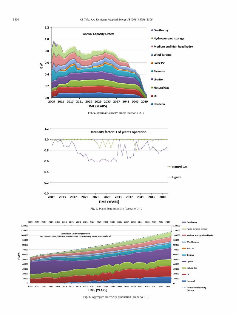
Fig. 6. Optimal Capacity orders (scenario D-I).

Fig. 7. Plants load intensity (scenario D-I).

Fig. 8. Aggregate electricity production (scenario D-I).


Fig. 9. Optimal capacity orders (scenario D-II).

Fig. 10. Plants load intensity (scenario D-II).

Fig. 11. Aggregate electricity production (scenario D-II).



orders) but on the other hand attempted to minimise the emissioncosts (by lowering the plants’ usage intensity). This counterbalanc-ing effect proves to be stronger in scenario D-II, as reflected in itslower h factor, by considering that the emission costs are proneto be relatively higher, due to the higher assumed CO2 allowanceprices of scenario D-II.

The above arguments may be further justified through the anal-ysis of Figs. 8 and 11, where the annual electricity production ispresented (scenarios D-I and D-II respectively). Some problemsmay be identified regarding a hypothetical broadening of renew-able energy penetration in electricity market. The long construc-tion periods of hydro-electric plants and the relatively lowcapacity factors of photovoltaic, hydroelectric and wind plantsinduce the requirement for very high installed capacities in orderto meet the demand targets. On the other hand, the investmentcosts of the above mentioned technologies – and in particular ofsolar energy technologies – are significantly high – despite theirState subsidisation – and may not favour renewable energy invest-ments. The above arguments are reflected to the annual capacityorders resulting from the optimisation algorithm, which are notas high as one might expect (Figs. 6 and 9). Moreover, the renew-able energy generation (shown in Figs. 8 and 11) barely manages tomeet its lower bound share in the electricity market (>30% afterthe year 2020 as stated in the EU directive 2001/77/EC). It alsostays far away from reaching the upper bound target determinedby the requirements for the grid stability (50% of total electricitydemand as described in Eq. (12)). Therefore, the renewable energytechnologies are challenged to the power sector domination raceand may not gain a higher market share unless the experience ac-quired in the distant future contributes to the further reduction oftheir investment costs. Despite their obvious environmentaladvantages, the renewable energy technologies may not be pro-moted under the current CO2 allowance prices, which might haveto be strengthened, thus forming an attractive condition for inves-tors willing to engage in this market. The reduction of investmentcosts due to the expected experience from future constructions ormarket competition may be a matter of time, whilst on the otherhand, the determination of CO2 allowance prices may not dependonly on allowances’ market dynamics but it may rather be a conse-quence of environmental policy interventions. Nonetheless, therenewable energy technologies are currently favoured by theirlow (or zero) fuel cost, which constitutes their sole significant pro-moting factor.

Of particular interest might be the exploitation of biomass feed-stocks, which are cheap and readily available in the domestic fuelmarket. Agricultural crops like cotton, corn, wheat etc. which arecultivated and grow in many rural areas of Greece might becomean alternative to the conventional energy production. Nonetheless,the complicated supply chains as well as life-cycle, logistical andorganisational issues should prior be resolved. Probably they couldnot replace natural gas as a base-load fuel, but their neutral CO2

emissions and the relatively high capacity factors render this tech-nology as a candidate alternative needing additional focus for theoncoming decade (Figs. 6 and 9).

The required policy interventions should be incorporated in thefuture power generation licence calls released by the State. Theyshould aim at high percentage of renewable energies (hydro-plants, wind turbines and biomass) in the first 3–4 years of imple-mentation of the program in order to put a basis for meeting theenvironmental directive targets. Some kWh subsidising policiesshould probably be considered for the promotion of renewableenergies during these first years of the program. From this pointforward, the distribution of capacity orders for power plants basedon combustion technologies (natural gas, lignite and biomass)should be balanced, whilst the capacity orders of solar PVs, windparks and hydro plants (either of hydro pumped storage or of med-

ium and high head hydro plants) should be reduced. As the totalinstalled capacities gradually rise over time, the environmentalconstraints impose the requirement for decreased usage of conven-tional lignite plants (characterised by high emission factors), thusenabling the minimisation of aggregate system emissions. Theabove rationale should be followed in the future licensing proce-dures, irrespective of the pricing model. Nonetheless, individualpower plants should take it into account, in order to remain com-petitive and keep up with current market trends – as far as theirown potential expansion planning is concerned. It is noted thatthe pricing model seems to impact, basically, the comparative scaleof the interventions but not their qualitative characteristics.

5.2. Dependency from uncertainties and installed generation mix

The expansion planning may depend on the multiple effects ofthe uncertainties as well as on the diversification of the installedgeneration mix. More specifically the results of the model, whichessentially depend on the input state, may not be valid for the entirefuture horizon. This problem might be attributed to the progres-sively increasing uncertainty characterising long-term randomwalk simulations. Moreover, the effect of the long times requiredfor the construction, setup and commissioning of each plant typeshould be accounted, thus complicating the determination of thevalid time-period of the results. Therefore, despite the fact thatthe scope of the work spans to the next 25 years, the optimisationalgorithm was allowed to run for an extended time-period of42 years, in an attempt to smoothly absorb the above mentionedboundary timing effects. Furthermore, the uncertainties’ modellingmay not represent the real future evolution of the correspondingstochastic variables. It rather projects their past behaviour by sam-pling the underlying noise through probability distributions deter-mined by recent historical data. This inherent limitation shoulddefinitely be accounted during any decision making process.

Interestingly, non-smooth variations of the capacity orders havebeen derived from the optimisation, despite that the oppositemight be expected for progressive time spots. Moderately smoothdistributions of optimal plant loads (h factors) were also producedover time. The variations of the corresponding graphs may be par-tially attributed to the non-stationary evolution of the forwardelectricity and fuel prices, as indicated by their simulated projec-tions. In a similar vein, the volatile evolution paths of the CO2

allowance prices and of the discounting factors can further justifythe above non-smooth distributions. The capacity orders requiredfor the displacement of obsolete plants (mainly of the workhorselignite-fired plants), also contribute to non-uniform results, as longas the end of their operation life signals massive capacity orders tomeet the demand targets, thus resulting to non-smooth orders’ dis-tribution. This may be characterised as a moderate drawback ofdiscrete – or quasi-continuous treatment, especially when expan-sion planning is modelled on an annual basis.

6. Statistical analysis

The proposed method could be validated by comparing the cor-responding results from several studies. However, on the one handthere is no similar research concerning the Greek Power Sector; onthe other hand, there were no readily available input data fromother countries, which would allow the processing of their portfo-lio planning and/or the comparison with other power sectors.Moreover, it might be hard enough to establish solid qualitativeor quantitative criteria which may potentially allow a direct com-parison with other similar researches referring to power sectorswith essentially different structures. Although the proposed modelmay be able to capture the different characteristics (or structure) of

Fig. 12. Convergence history for scenario A-I.

Fig. 13. Normal distribution fitting of actual electricity demand data (daily basis).


various power sectors, a statistical analysis of the results is used in-stead, for the assessment of the suggested approach.

6.1. Convergence history of the optimisation algorithm

The convergence history of the algorithm is comprised of theobjective function differences (between successive iterations) untila very small value (e) is obtained. Indicatively, the convergence his-

tory of the scenario A-I is presented in Fig. 12. An initial state hasbeen introduced in the algorithm, based on a moderate evolutionof the current generation mix. In the first steps of the iterative pro-cedure, the suboptimal NPV values deviate significantly from theoptimal value. This is finally converged to the level of 52.109 Euros(also shown in Fig. 4) indicating a significant improvement com-pared to the initial NPV. Negative NPV values are progressivelyiterated as the algorithm was built to seek for minimum values.

Fig. 14. Log-normal distribution fitting of the multiple GBM solutions for a future time-point.


Therefore, if a maximisation is required, the negative of the NPVobjective function should be derived.

6.2. Deviation from the constraints

The cumulative energy production shown in Figs. 8 and 11 indi-cates a minimal deviation from the energy demand as imposed inthe relevant constraints (Eqs. (11a) and (11b)). Their coincidenceensures meeting the demand target with minimal aggregate costs.

6.3. Error analysis

The comparison of the simulated with the actual data was per-formed using the median absolute deviation (MAD) as a measure oferror. The MAD indicator is defined as follows:

MAD ¼ median½dz;f �medianðdz;aÞ� ð17Þ

The analysis was performed using the – daily recorded – data of en-ergy demand for the years 2000–2009. This period was split in twodiscrete time-frames: 2000–2005 and 2006–2009. The first set wasused as a sample set needed for the random walk simulation whilstthe second was used for the validation of the resulting forecasts forthe corresponding years (2006–2009). The comparison lead to anerror with MAD = 11.5% of the average observations recorded inthe validation data-set, thus reflecting a relatively accurate forecast.It is noted though that the random walk forecast is characterised byprogressively increasing statistical uncertainty. In order to calculatethis uncertainty a statistical analysis is required. Primary objectiveof this statistical analysis is the determination of the statistical dis-tribution of the original (historical) data. The demand data may beconsidered as normally distributed, as shown in the observationsstatistical fitting (Fig. 13).

The determination of the uncertainty is possible by assumingnormally distributed Brownian differentials and a requirementfor a confidence interval (CI) equal to 95%. According to theory[36], when the Brownian differentials are normally distributedthe resulting GBM simulation comprises of log-normally distrib-uted solutions. These are characterised by progressively increasingconfidence limits over time – for a given CI – and may significantlydeviate from the forecast especially in the distant future. The con-

fidence limits of the aggregate annual demand forecasts are plottedin Fig. 1 (assuming CI = 95%). The lognormal distribution fitting ofan indicative time-point of the GBM solution is shown in Fig. 14.

The mean value is extracted by the lognormal distribution forthis time point, forming an average forecast. The same procedureis performed for the calculation of the confidence limits of theremaining stochastic variables. It is noted that adequate iterationsof this Monte-Carlo procedure are required until the confidencelimits cannot be further reduced for an assumed CI.

7. Conclusions

In this article, the impact of electricity and CO2 allowance pricesis investigated within the framework of electricity productionportfolios. The numerical experiments conducted, focused on theoptimisation of the power sector structure over time. The GreekPower Sector was introduced as the case-study market under mul-tiple uncertainties. The electricity demand, the forward prices ofelectricity, the CO2 allowance prices as well as the fuel prices wereconsidered as stochastically evolving. The evolutions of interestand inflation rates were represented through stochastic processesas well, thus minimising the requirement for arbitrary riskassumptions. The iterative optimisation algorithm attempted tomaximise the system NPV whilst being subject to various social,supply and demand constraints. Constraints related with the avail-ability of natural resources, the stability of the national grid oper-ation and the environmental directives were additionally imposed.A stochastic programming approach without recourse was used,incorporating an SQP numerical solver.

The results of the optimisation focus on the annual capacityadditions, the plant loads and the corresponding energy produc-tion required from each technology. A significant improvementmay be identified in respect of the iterated system NPVs and theanticipated CO2 emissions over time. More specifically, the algo-rithm tends to maximise the system NPV by iteratively attemptingto reduce the overall system costs and the CO2 emission costs inparticular, thus minimising the anticipated CO2 emissions as well.The resulting generation mix (suggested for the medium-termexpansion planning of the Greek Power Sector) shows that theCO2 emissions per unit of electricity might be reduced by 30%


within the next 25 years. The analysis of the results indicates thathigher electricity prices may be proportionally beneficial for thefinancial yields of the power sector. On the other hand, the CO2

allowance prices may be inversely proportionate with the expectedyields and with the anticipated CO2 emissions over time, thusforming an inhibitor for capacity orders from conventionaltechnologies.

The combined influence of the various commodities underuncertainty may marginally be explained in an empirical way asthe results are derived through complex algorithmic optimisationprocesses. Nonetheless, they could provide useful information byfocusing on specific time spots, thus identifying particularly inter-esting investment opportunities. If these opportunities are suppos-edly bypassed (investments realised in suboptimal time-windows)there may be fewer chances for individual players to be profitable.Therefore, the hypothetical investors might have to be aware of theupper bound share of each technology. Their subsequent decisionsshould be probably reconsidered according to current markettrends, fiscal conditions and competition. Moreover, their decisionsshould be further evaluated in conjunction with standard licensingpractices, periodically applied by the State during expansion plan-ning, thus complying with the relevant policy interventions, whichdetermine the bounds of capacity shares. This strategy mightpotentially contribute to the reduction of the social cost as wellas to more favourable effects on the sustainability of the system.

NPVðXi¼1;v ; . . . ;Xi¼I;v ; hi¼1;z; . . . ; hi¼I;zÞ ¼max

PI

i¼1

PYz¼1

pezDzPz�Tli

v¼1Xi;v þ

P0v¼�40

Ci;v �Pzv¼1

Xi;v �P0

v¼�40Ci;v

!hi;zaa;iac;i � 8760�

�PI

i¼1

PYz¼1

Cfi;zDzPz�Tli

v¼1Xi;v þ

P0v¼�40

Ci;v �Pzv¼1

Xi;v �P0

v¼�40Ci;v


�PI

i¼1

PYz¼1

Cv i;zDzPz�Tli

v¼1Xi;v þ

P0v¼�40

Ci;v �Pzv¼1

Xi;v �P0

v¼�40Ci;v

!�

�PYv¼0

PI

i¼1Ii;vXi;v�

�PI�RE

i¼1

PYz¼1

Pz�Tli

v¼1Xi;v þ

P0v¼�40

Ci;v �Pzv¼1

Xi;v �P0

v¼�40Ci;v

!hi;zaa;iac;i � 8760 � fCO2i

ni� Dz � pCO2z

þ

þPRE

i¼1

PYz¼1

Pz�Tli

v¼1Xi;v þ

P0v¼�40

Ci;v �Pzv¼1

Xi;v �P0

v¼�40Ci;v


�PI�RE

i¼1ECO2iPI�RE

i¼1

Pz�Tliv¼1

Xi;vþP0

v¼�40Ci;v�

Pz

v¼1Xi;v�

P0

v¼�40Ci;v

� �hi;zaa;iac;i �8760

� Dz � pCO2z

8>>>>>>>>>>>>>>>>>>>>>>>>>>>>>>>><>>>>>>>>>>>>>>>>>>>>>>>>>>>>>>>>:

9>>>>>>>>>>>>>>>>>>>>>>>>>>>>>>>>=>>>>>>>>>>>>>>>>>>>>>>>>>>>>>>>>;

ðA5Þ

Appendix A

A general optimisation problem may be formulated as follows:

min jxf ðxÞsubject to the constraints :

CiðxÞ ¼ 0; 8i ¼ 1; . . . ; ke

CiðxÞ 6 0; 8i ¼ ke þ 1; . . . ; k

ðA1Þ

where (x) is the independent variables vector of length k, f(x) is theobjective function, which returns a scalar value, and the vectorfunction C(x) returns a vector of length k containing the values ofthe equality and inequality constraints evaluated at x. TheKaroush–Kuhn–Tucker equations (KKT) can be described by thefollowing:

rf ðxÞ þPki¼1

ki � rCiðxÞ ¼ 0

ki � rCiðxÞ ¼ 0; 8i ¼ 1; . . . ; ke

ki P 0; 8i ¼ ke þ 1; . . . ; k

ðA2Þ

It is noted that the KKT equations include the constraints set ofEq. (A1). The principal idea for convergence in the SQP algorithmsis the construction of a quadratic sub-problem based on a qua-dratic approximation of the Lagrangian function:

Lðx; kÞ ¼ f ðxÞ þXk

i¼1

ki � ciðxÞ ðA3Þ

By assuming that boundary constraints have been expressed asinequality constraints, the QP sub-problem may be obtained by lin-earising the nonlinear constraints:

min jd2Rn12 dT Hkdþrf ðxkÞd

rciðxkÞT dþ ciðxkÞ ¼ 0; 8i ¼ 1; . . . ; ke

rciðxkÞT dþ ciðxkÞ 6 0; 8i ¼ ke þ 1; . . . ; k

ðA4Þ

where Hk denotes the Hessian matrix of the quadratic approxima-tion and d denotes the updates solutions vector. The objective func-tion of the present research may be formulated by combining Eqs.(4)–(6) (described in the main text):

It represents an analytical relationship of the final NPV with therequested optimal capacity orders and the usage intensities of thepower plants during the entire period of investigation. A doublesweeping in respect of time is implemented: the first one scansthe lead-times and the second sweeps over the operational life-time. An additional third sweeping direction through the compet-ing technologies is additionally implemented. The uncertainties ofNPV function are comprised of the forward electricity prices (pez),the electricity demand (dz,f), the CO2 allowance prices (pCO2,z) andthe fuel prices (Cfi,z). The corresponding paths are calculated usingthe stochastic models described by Eq. (1), whilst the discountingfactors (Dz) are calculated using the stochastic differential equa-tions. (2) combined with Eq. (3). The above uncertainty sets areintroduced as inputs in the optimisation problem (A1)–(A5) usingthe objective function (Eq. (A5)).


References

[1] Aki H, Oyama T, Tsuji K. Analysis of energy service systems in urban areas andtheir CO2 mitigations and economic impacts. Appl Energy2006;83(10):1076–88.

[2] Siitonen S, Tuomaala M, Suominen M, Ahtila P. Implications of process energyefficiency improvements for primary energy consumption and CO2 emissionsat the national level, Appl Energy 87(9). Special Issue of the IGEC-IV, the 4thInternational Green Energy Conference (IGEC-IV), Beijing, China, October 20-22, 2008; Special Issue of the First International Conference on Applied Energy,ICAE’09, Hong Kong, January 5–7, 2009, September 2010. p. 2928–37.

[3] Bar-Lev D, Katz S. A portfolio approach to fossil fuel procurement in the electricutility industry. J Finance 1976;31:933–47.

[4] Awerbuch S. Portfolio-based electricity generation planning: policyimplications for renewables and energy security. Mitig Adapt Strat GlobChange 2006;11:693–710.

[5] Awerbuch S, Berger M. Energy security and diversity in the EU: a mean–variance portfolio approach. Paris: International Energy Agency; 2003.

[6] Bazilian M, Roques F. Analytic methods for energy diversity and security.Applications of mean variance portfolio theory. A tribute to shimonawerbuch. London: Elsevier; 2008.

[7] Fortin I, Fuss S, Hlouskova J, Khabarov N, Obersteiner M, Szolgayova J. Anintegrated CVaR and real options approach to investments in the energy sector.J Energy Mark 2008;1:61–85.

[8] Roques FA, Newberry DM, Nuttall WJ. Fuel mix diversification incentives inliberalized electricity markets: a mean–variance portfolio theory approach.Energy Econ 2008;30:1831–49.

[9] Huisman R, Mahieu R, Schlichter F. Electricity portfolio management: optimalpeak/off-peak allocations. Energy Econ 2009;31(1):169–74.

[10] Huang Y, Wu J. A portfolio risk analysis on electricity supply planning. EnergyPolicy 2009;37(2):744–61.

[11] Svensson E, Berntsson T, Strömberg AB, Patriksson M. An optimisationmethodology for identifying robust process integration investments underuncertainty. Energy Policy 2009;37(2):680–5.

[12] Vahidinasab V, Jadid S. Multi-objective environmental/techno-economicapproach for strategic bidding in energy markets. Appl Energy2009;86(4):496–504.

[13] Heinrich G, Howells M, Basson L, Petrie J. Electricity supply industry modellingfor multiple objectives under demand growth uncertainty. Energy2007;32(11):2210–29.

[14] Krey V, Martinsen D, Wagner HJ. Effects of stochastic energy prices on long-term energy-economic scenarios. Energy 2007;32(12):2340–9.

[15] Turton H. ECLIPSE: an integrated energy-economy model for climate policyand scenario analysis. Energy 2008;33(12):1754–69.

[16] Keppo J, Lu H. Real options and a large producer: the case of electricitymarkets. Energy Econ 2003;25:459–72.

[17] Laurikka H, Koljonen T. Emissions trading and investment decisions in thepower sector – a case study of Finland. Energy Policy 2006;34:1063–74.

[18] Laurikka H. Option value of gasification technology within an emissionstrading scheme. Energy Policy 2006;34(18):3916–28.

[19] Madlener R, Kumbaroglu G, Ediger V. Modelling technology adoption as anirreversible investment under uncertainty: the case of the Turkish electricitysupply industry. Energy Econ 2005;27:39–163.

[20] Xia Y, Zhao YD, Saha TK. Optimal portfolio selection for generators in theelectricity market. Power and energy society general meeting – conversion anddelivery of electrical energy in the 21st Century. IEEE; 2008. p. 1–7.

[21] Kumbaroglu G, Madlener R, Demirel M. A real options evaluation model for thediffusion prospects of new renewable power generation technologies. EnergyEcon 2008;30:1882–908.

[22] Nocedal J, Wright SJ. Numerical optimization. Springer series in operationsresearch. Springer Verlag; 1999.

[23] Conn NR, Gould NIM, Toint PhL. Trust-region methods. MPS/SIAM series onoptimization, SIAM and MPS; 2000.

[24] Schittkowski K. NLQPL: a FORTRAN-subroutine solving constrained nonlinearprogramming problems. Ann Oper Res 1985;5:485–500.

[25] Fletcher R. Practical methods of optimization. John Wiley and Sons; 1987.[26] Biggs M, Hernandez M. Using the KKT matrix in an augmented Lagrangian SQP

method for sparse constrained optimisation. J Optim Theory Appl1995;85:201–20.

[27] Mo B, Hegge J, Wangensteen I. Stochastic generation expansion planning bymeans of stochastic dynamic programming. IEEE Trans Power Syst1991;6(2):662–8.

[28] Tanabe R, Yasuda K, Yokoyama R, Sasaki H. Flexible generation mix undermultiple objectives and uncertainties. IEEE Trans Power Syst 1993;8(2):581–7.

[29] Box G, Jenkins J, Reinsel G. Time series analysis: forecasting and control. 3rded. Upper Saddle River (NJ): Prentice Hall; 1994.

[30] Øksendal B. Stochastic differential equations. Springer-Verlag; 2000.

[31] Vasicek O. An equilibrium characterisation of the term structure. J Financ Econ1977;5:177–88.

[32] Cox JC, Ingersoll JE, Ross SA. A theory of the term structure of interest rates.Econometrica 1985;3(2):385–407.

[33] Ingersoll JE, Ross SA. Waiting to invest: investment and uncertainty. J Bus1992;65(1):1–29.

[34] Kloeden PE, Platen E. Numerical solution of stochastic differentialequations. Berlin: Springer; 1999.

[35] Shreve R. Stochastic calculus for finance II: continuous-time models. Springer-Verlag; 2004.

[36] Glasserman G. Monte-Carlo methods in financial engineering. Springer-Verlag;2004.

[37] Fleten SE, Maribu K, Wangensteen I. Optimal investment strategies indecentralized renewable power generation under uncertainty. Energy2007;32:803–15.

[38] Fuss S, Johansson D, Szolgayova J, Obersteiner M. Impact of climate policyuncertainty on the adoption of electricity generating technologies. EnergyPolicy 2009;37(2):733–43.

[39] Li YP, Huang GH, Chen X. Planning regional energy system in association withgreenhouse gas mitigation under uncertainty. Appl Energy2011;88(3):599–611.

[40] Zhou W, Zhu B, Fuss S, Szolgayova J, Obersteiner M, Fei W. Uncertaintymodeling of CCS investment strategy in China’s power sector. Appl Energy2010;87(7):2392–400.

[41] Fuss S, Szolgayova J, Obersteiner M, Gusti M. Investment under market andclimate policy uncertainty. Appl Energy 2008;85(8):708–21.

[42] Deng S, Oren S. Incorporating operational characteristics and start-up costs inoption based valuation of power generation capacity. Probab Eng Inf Sci2003;17:155–81.

[43] Tolis A, Doukelis A, Tatsiopoulos I. Stochastic interest rates in the analysis ofenergy investments: implications on economic performance andsustainability. Appl Energy 2010;87(8):2479–90.

[44] Dias JC, Shackleton MB. Investment hysteresis under stochastic interest rates.In: 9th Annual international conference on real options. Paris; 2005.

[45] Yang M, Blyth W, Bradley R, Bunn D, Clarke C, Wilson T. Evaluating the powerinvestment options with uncertainty in climate policy. Energy Econ2008;30:1933–50.

[46] Junginger M, Faaij A, Turkenburg WC. Global experience curves for wind farms.Energy Policy 2005;33(2):133–50.

[47] Rubin ES. Learning rates and future cost of power plants with CO2 capture. In:IEA international workshop on technology learning and deployment. Paris;2007.

[48] Botterud A, Korpas M. A stochastic dynamic model for optimal timing ofinvestments in new generation capacity in restructured power systems. ElectrPower Energy Syst 2007;29(2):163–74.

[49] HTSO S.A. Hellenic transmission system operator. statistics for the years 2001–2009. HTSO; 2009. <www.desmie.gr> [13.11.09].

[50] Barlow MT. A diffusion model for electricity prices. Math Finance2002;12(4):287–98.

[51] Audet N, Heiskanen P, Keppo J, Vehvilainen I. Modelling electricity forwardcurve dynamics in the Nordic market. In: Bunn DW, editor. Modelling prices incompetitive electricity markets. New York: Wiley Series in FinancialEconomics; 2003.

[52] Dixit A, Pindyck R. Investment under uncertainty. Princeton: PrincetonUniversity Press; 1994.

[53] Clewlow L, Strickland C. Energy derivatives: pricing and riskmanagement. London: Lacima Publications; 2000.

[54] Weigt H. Germany’s wind energy: the potential for fossil capacity replacementand cost saving. Appl Energy 2009;86(10):1857–63.

[55] Zhang Y, Wei Y. An overview of current research on EU ETS: evidence from itsoperating mechanism and economic effect. Appl Energy 2010;87(6):1804–14.

[56] Greek ministry of development. YPAN; 2009. <www.ypan.gr> [10.11.09].[57] General secretariat of national statistical service of Greece. ESYE; 2009.

<www.statistics.gr> [17.11.09].[58] Natural gas company of Attica. Statistics for the years 2001–2008. DEPA; 2009.

<http://www.aerioattikis.gr/> [15.11.09].[59] International energy agency. 2008. Statistics for Greece. IEA; 2008.

<www.iea.org> [11.08.09].[60] Point-carbon. Carbon market indicator; 2009. <http://www.pointcarbon.com>

[14.11.09].[61] Tatsiopoulos I, Tolis A. Economic aspects of the cotton-stalk biomass logistics

and comparison of supply chain methods. Biomass Bioenerg J2003;24:199–214.

[62] Aid R, Campi L, Nguyen HA, Touzi N. A structural risk-neutral model ofelectricity prices. HAL-CCSD; 2009. Working papers, HAL. <http://econpapers.repec.org/RePEc:hal:wpaper:hal-00390690_v2>.

http://www.desmie.gr

http://www.ypan.gr

http://www.statistics.gr

http://www.aerioattikis.gr/

http://www.iea.org

http://www.pointcarbon.com

http://econpapers.repec.org/RePEc:hal:wpaper:hal-00390690_v2

http://econpapers.repec.org/RePEc:hal:wpaper:hal-00390690_v2

An impact assessment of electricity and emission allowances pricing in optimised expansion planning...

Documents

Transcript of An impact assessment of electricity and emission allowances pricing in optimised expansion planning...