
An economic view of carbon allowances market
36
Documents de Travail du Centre d’Economie de la Sorbonne An economic view of carbon allowances market Marius-Cristian FRUNZA, Dominique GUEGAN 2009.38 Maison des Sciences Économiques, 106-112 boulevard de L'Hôpital, 75647 Paris Cedex 13 http://ces.univ-paris1.fr/cesdp/CES-docs.htm ISSN : 1955-611X halshs-00390676, version 1 - 2 Jun 2009
-
Upload
polytechnique -
Category
Documents
-
view
8 -
download
0
Transcript of An economic view of carbon allowances market
Documents de Travail duCentre d’Economie de la Sorbonne
An economic view of carbon allowances market
Marius-Cristian FRUNZA, Dominique GUEGAN
2009.38
Maison des Sciences Économiques, 106-112 boulevard de L'Hôpital, 75647 Paris Cedex 13http://ces.univ-paris1.fr/cesdp/CES-docs.htm
ISSN : 1955-611X
hals
hs-0
0390
676,
ver
sion
1 -
2 Ju
n 20
09

AN ECONOMIC VIEW OF CARBON ALLOWANCES MARKET
MARIUS-CRISTIAN FRUNZA*, DOMINIQUE GUEGAN**
Abstract. The aim of this work is to bring an econometric approach upon
the CO2 market. We identify the specificities of this market, and regarding the
carbon as a commodity. We investigate the econometric particularities of CO2
prices behavior and their result of the calibration. We apprehend and explain
the reasons of the non-Gaussian behavior of this market focusing mainly upon
jump diffusion and generalized hyperbolic distributions. We test these results
for the risk modeling of a structured product specific to the carbon market,
the swap between two carbon instruments: the European Union Allowances
and the Certified Emission Reductions. We estimate the counterparty risk for
this kind of transaction and evaluate the impact of different models upon the
risk measure and the allocated capital.
1. Introduction
Human activities, in particular the population growth and the development of
industry over the last 200 years, have caused an increase in the emission and atmo-
spheric concentration of certain gases, called ”greenhouse gases” - primarily carbon
dioxide and methane. These gases intensify the natural greenhouse effect that
occurs on Earth, which in itself allows life to exist. The man-induced enhanced
greenhouse effect leads to an increase in the average temperature of the planet
that, would potentially cause increasingly severe and perhaps even more extreme
disruptions to the Earth’s climate, and consequently human activity.
Key words and phrases. Carbon, Normal Inverse Gaussian, CER, EUA, swap.* CES, University Paris 1 Pantheon-Sorbonne; Sagacarbon, 67 rue de l’Universite, 75007, Paris,
[email protected].** PSE, CES-MSE, University Paris 1 Pantheon-Sorbonne, 106 Bd de l’Hopital,75013, Paris,
1
Document de Travail du Centre d'Economie de la Sorbonne - 2009.38
hals
hs-0
0390
676,
ver
sion
1 -
2 Ju
n 20
09

2 MARIUS-CRISTIAN FRUNZA*, DOMINIQUE GUEGAN**
As a consequence several governments, firms and individuals have taken steps
to reduce their greenhouse gas (GHG) emissions either voluntarily, or, increasingly,
because of current or expected regulatory constraints.
With its ratification by Russia in early 2005 the Kyoto protocol became an
international law. According to its provisions, the industrialized countries have to
reduce in the period 2008-2012 the greenhouse gas emissions by 5 percent with
respect to the 1990 year levels.
The protocol dictates the trading of emission allowances as one of the primary
mechanisms through which greenhouse gas emission reduction should be achieved.
Thus, the right to pollute is considered to be a tradable asset, with its price deter-
mined by the market forces of supply and demand.
The European Union has agreed under the Kyoto Protocol to reduce its green-
house gas emissions in the period 2008 - 2012 by 8 percent with respect to the 1990
year levels. The adopted strategy for meeting this target is the establishment of a
European wide emission allowance market, the European Union Emission Trading
Scheme (EU ETS) that was initiated on January 2005. The EU ETS is considered
to be the largest single market for emission allowance trading, representing in 2007
approximatively 45 billion euros.
The carbon market encompasses both project-based emission reduction transac-
tions and emissions trading of GHG emission allowances. The first one concerns
the purchase of emission reductions (ERs) from a project which reduces green-
house gases emissions compared with what would have happened otherwise. The
second one concerns the allowances that are allocated under existing or upcoming
cap-and-trade regimes.
In this paper, we define carbon transactions as contracts whereby one party
pays another party in exchange for a given quantity of GHG emissions credits
that the buyer can use to meet its objectives vis-a-vis climate mitigation. Carbon
transactions can be grouped in two main categories:
Document de Travail du Centre d'Economie de la Sorbonne - 2009.38
hals
hs-0
0390
676,
ver
sion
1 -
2 Ju
n 20
09
AN ECONOMIC VIEW OF CARBON ALLOWANCES MARKET 3
• Trades of emission allowances, such as, for example, Assigned Amount Units
(AAUs) under the Kyoto Protocol, or allowances under the EU Trading
Scheme (EUAs). These allowances are created and allocated by a regulator,
usually under a cap-and-trade regime;• Project-based transactions, that is, transactions in which the buyer partici-
pates in the financing of a project which reduces GHG emissions comparedwhich what would have happened otherwise, and get emission credits inreturn. Unlike allowance trading, a project-based transactions can occureven in the absence of a regulatory regime: an agreement between a buyerand a seller is sufficient.
In some recent works, few authors Benz [2], Daskalakis and Markellos [5],[6],
Homburg [16] and Paolella [13] focused on the econometrical modeling of the GHG
prices, underlying the particularities of this market like the non-Gaussian behavior,
the auto-regressive phenomena and the presence of the convenience yield. In the
present paper we consider a new class of models based on generalized hyperbolic
distributions and we apply the results of prices calibration to a financial product
specific to the CO2 market, the carbon arbitrage.
In order to have an econometric view of the GHG market we calibrated EUAS
prices behavior using both Brownian and generalized hyperbolic models. We tested
also the changing regimes hypothesis by integrating jumps in our diffusion models.
In the first section of this paper we focus mainly on the main features of the
GHG market: the efficient market hypothesis, the resemblance to commodities,
the convenience yield and the non-Gaussian behavior. The second section concerns
the calibration of the econometric models based on Gaussian diffusion (Geomet-
ric Brownian diffusion, Mean reverse Brownian Diffusion, Brownian Jump diffusion
and Mean reverse Brownian diffusion with jumps) and Generalized Hyperbolic (GH)
distributions (Normal Inverse Gaussian distribution and Normal Inverse Gaussian-
Brownian mixture). Section three emphasizes the applications of the previous sec-
tions on the risk measure of a structured product typical to carbon market the
swap between two carbon instruments: the EUAs and the CERs. We benchmark
Document de Travail du Centre d'Economie de la Sorbonne - 2009.38
hals
hs-0
0390
676,
ver
sion
1 -
2 Ju
n 20
09

4 MARIUS-CRISTIAN FRUNZA*, DOMINIQUE GUEGAN**
the different models in order to identify the strengths and the weaknesses of each
model. In section four we underline the main conclusions of our study.
2. Overview of GHG trading prices
As a direct consequence of the Kyoto protocol implementation spot quotations
were launched on Powernext in June 2005, but was interrupted at the end of Decem-
ber 2007 because of transferring the CO2 trading activities on the Nyse-Euronext
platform. Today (at the end of December 2008), spot transactions have began on
the BlueNext market, only since early 2008. This means that we had to recon-
struct spot prices using ”futures” contracts quoted on ECX, for the two previous
years. Moreover, long-term ECX futures contracts are not liquid enough, which
means that we had to check the relevance of quotations and adjust data if neces-
sary. Based on these facts we develop some reflections about the carbon around
four topics: efficient market hypothesis (EMH), commodity likeliness, convenience
yield and non-Gaussian behavior.
2.1. The efficient market hypothesis. The EMH is a common assumption in
traditional financial economics. In its weak form EMH implies that the changes in
financial time series (e.g., equity prices, interest rates, exchange rates) are white
noise processes consisting of independent, identically distributed random variables.
These assumptions imply that the time series follow random walks. One of the
main empirical characteristics of financial assets’ yields is the dynamic evolution of
their volatilities.
The European GHG emission allowances market (EUA) is a direct consequence
of a regulatory system commonly accepted by the market actors. Some sources of
market inefficiency do exist:
• the new information is unequally diffused amongst market players. In fact
some of the companies submitted to Kyoto protocol (ie. Vatenfall, Mittal...)
or funds involved in quota/credit trading (ie. European Carbon Fund) are
in same time investors and clients. Given their positions these players
Document de Travail du Centre d'Economie de la Sorbonne - 2009.38
hals
hs-0
0390
676,
ver
sion
1 -
2 Ju
n 20
09
AN ECONOMIC VIEW OF CARBON ALLOWANCES MARKET 5
possess more information about the current status of the market than their
peers. This informational dissymmetry weakens the efficiency hypothesis
of GHG allowance market ;
• the EUA is perceived mainly as a financial liability and has not any intrinsic
value capable of generating economic added value for an investor;
• both price and volatility are driven with a high impact by regulatory an-
nounces. Regulatory changes can modify the behavior of the market and
bring the exchange system in a completely different regime (ie. may 2006);
• the EUA system is a dealer market. The European Carbon Exchange pro-
vides liquidity to investors by trading shares for themselves. Therefore we
observe periods were the price is given by the market even if no trade exist.
The advantage of having a continuous quotation has an obvious downside
of irrelevant values over periods of low liquidity.
As a new market with only three years of history, the GHG emission allowances
show a particular behavior due to small trading volumes, relative small number of
market actors and regulatory pressure.
For example EUA 2008 and 2009 historical prices (Figure1) exhibit high vari-
ability regimes and discontinuities in offer/demand equilibrium. For a significant
number of trading days the exchanged volumes of contracts are very small or even
zero. In those particular days the prices are marked by the auction trading systems.
Nevertheless those data are not relevant for statistical estimations due to the fact
that they do not reflect a market equilibrium state.
A way to test efficiency of securities market is to search for autocorrelation
and implicitly for persistence in yield and volatility levels. In order to deal with a
possible lack of efficiency on the GHG allowance market we will search of persistence
evidence and correlated phenomena.
We used the most recent 990 daily negative log return data of EUA08 (Figure1)
to plot the sample autocorrelation function (ACF). From Figure 2, we can see that
Document de Travail du Centre d'Economie de la Sorbonne - 2009.38
hals
hs-0
0390
676,
ver
sion
1 -
2 Ju
n 20
09

6 MARIUS-CRISTIAN FRUNZA*, DOMINIQUE GUEGAN**
Figure 1. EUA08 and EUA09 prices history
the ACF of the negative log return series shows little evidence of serial correlation,
while the ACF of squared return series does show evidence of serial dependence.
We observed also some relevant lags are shown for the first, sixth and thirteenth
days. Nevertheless we remarked a strong persistence phenomena on the squared
innovation time series before and after applying the linear filters.
2.2. Commodity likeliness: Between physical reality and metaphysical
concept. The term ”commodity” is commonly apprehended as a physical good,
such as food, oil, and metals, which is interchangeable with another good of the same
type, which is bought or sold by market players, usually through futures contracts.
More generally, a ”commodity” is a product which trades on a commodity exchange;
this would also include energy contracts.
On one hand, we could look at GHG allowance prices as a commodity represent-
ing the right to pollute the environment. This right is underwritten by governments
and given to different industries depending of their profile. In this case the price of
an allowance would represent the marginal cost of reducing the GHG emissions. In
Document de Travail du Centre d'Economie de la Sorbonne - 2009.38
hals
hs-0
0390
676,
ver
sion
1 -
2 Ju
n 20
09

AN ECONOMIC VIEW OF CARBON ALLOWANCES MARKET 7
Figure 2. Autocorrelation for EUA08 negative daily returns
an efficient market environment this cost could be traded between industries sub-
mitted to emission constraints. The price would be established depending on the
offer and the demand of the market. Thus, an independent investor would perceive
her money as working in a physical mechanism that reduces the emissions.
On the other hand, the allowances are imposed by governments in order to stim-
ulate the industries to reduce their emissions. If an industry has more allowances
than actual emissions it will cash them out on the market. If it is short of al-
lowances it will fill the need by buying it on the market. This kind of perception
would push an independent perception to perceive her money as being held in a
regulatory paper traded between industries without having behind any physical
mechanism. Thereby the price of this security will be determined by the difference
between allowed and real emissions of an industry.
2.3. Convenience yield. Commonly the convenience yield is a measure of the
added value or premium associated with holding an underlying product or physical
good, compared to the detention of the term contract (i.e. future, forward).
Document de Travail du Centre d'Economie de la Sorbonne - 2009.38
hals
hs-0
0390
676,
ver
sion
1 -
2 Ju
n 20
09
8 MARIUS-CRISTIAN FRUNZA*, DOMINIQUE GUEGAN**
Sometimes, due to irregular market movements such as an inverted market,
the holding of an underlying good or security may become more profitable than
owning the contract or derivative instrument, due to its relative scarcity versus
high demand.
An example would be purchasing physical bales of wheat rather than future con-
tracts. In the hypothesis of a sudden drought and the demand for wheat increases,
the difference between the first purchase price of the wheat versus the price after
the shock would be the convenience yield.
If we apprehend the GHG allowances as a classic commodity like oil, gas or gold
we should find similarities in the economic interpretation.
On the one hand, the agent has the option of flexibility with regards to con-
sumption (no risk of commodity shortage). On the other hand, the decision to
postpone consumption implies storage expenses. The net cost of these services per
unit of time is termed the convenience yield δ. Intuitively, the convenience yield
corresponds to dividend yield for stocks, thereby the price of a forward contract is
given by:
(2.3.1) Ft,T = St · exp((rt,T − δt,T ) · (T − t)),
where Ft,T is the value at the moment t of the future contract for the maturity
T , St is the spot value at the moment t, rt,T and δt,T are respectively the values of
the rate and convenience yield for the maturity T .
One point of focus would be the convenience yield perceived as the amount of
benefit that is associated with physically owning a particular good, rather than
owning a futures contract for that good. When a good is easy to come by, an
investor does not have need to own the actual good at that time, and can buy or
sell as he pleases. When there is a shortage of a particular good, however, it is
better to already own the good than to have to purchase it during the shortage
Document de Travail du Centre d'Economie de la Sorbonne - 2009.38
hals
hs-0
0390
676,
ver
sion
1 -
2 Ju
n 20
09
AN ECONOMIC VIEW OF CARBON ALLOWANCES MARKET 9
because it is likely to be at a higher price due to the demand. The convenience
yield is the benefit derived in the second scenario.
For example the quotas holders would not sell their quotas to realize an arbitrage
opportunity (by selling the quota and buying futures contracts). Consequently they
”value” their owner-right and the convenience yield is, then a major element while
modeling the GHG price.
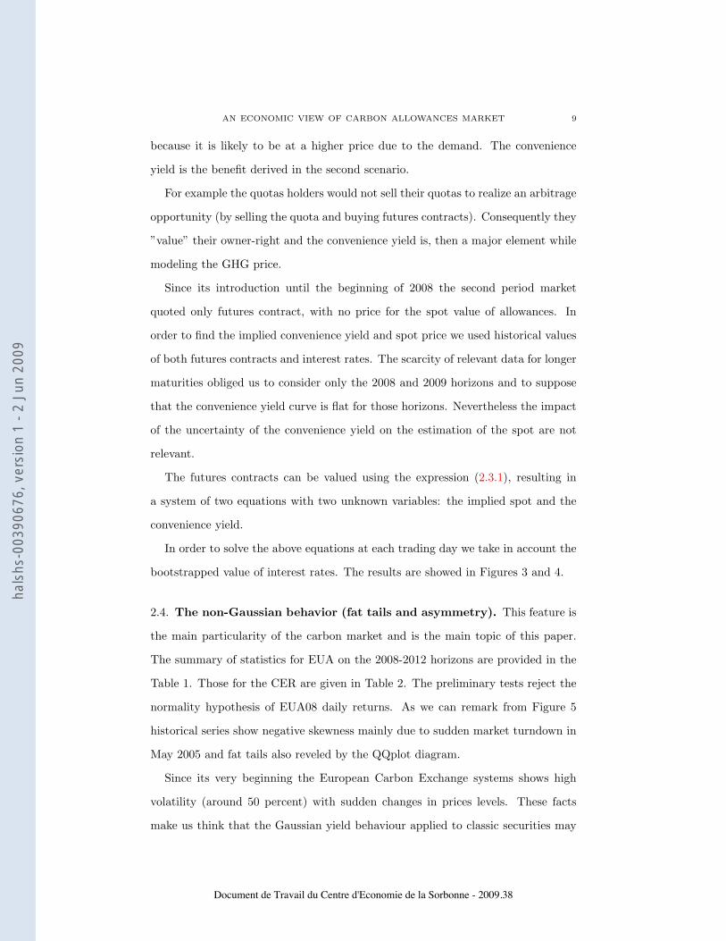
Since its introduction until the beginning of 2008 the second period market
quoted only futures contract, with no price for the spot value of allowances. In
order to find the implied convenience yield and spot price we used historical values
of both futures contracts and interest rates. The scarcity of relevant data for longer
maturities obliged us to consider only the 2008 and 2009 horizons and to suppose
that the convenience yield curve is flat for those horizons. Nevertheless the impact
of the uncertainty of the convenience yield on the estimation of the spot are not
relevant.
The futures contracts can be valued using the expression (2.3.1), resulting in
a system of two equations with two unknown variables: the implied spot and the
convenience yield.
In order to solve the above equations at each trading day we take in account the
bootstrapped value of interest rates. The results are showed in Figures 3 and 4.
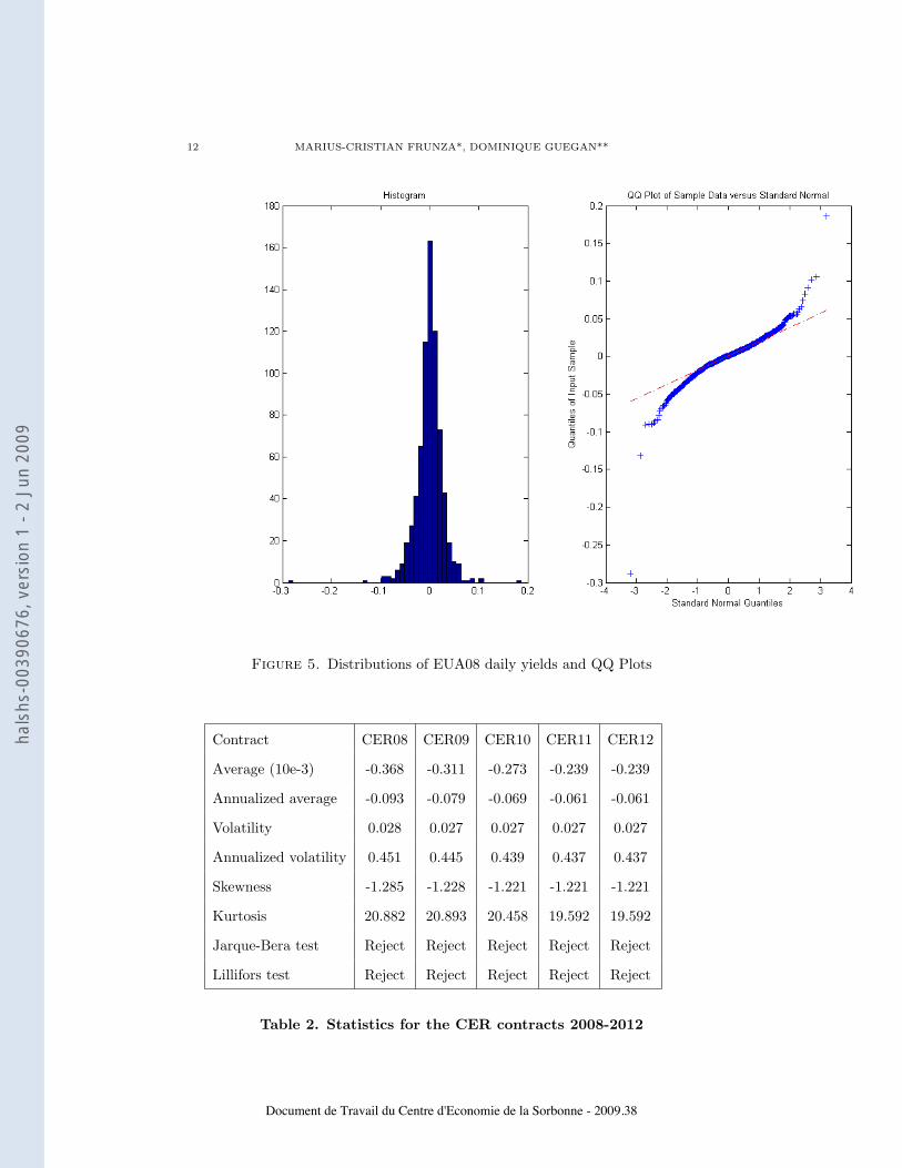
2.4. The non-Gaussian behavior (fat tails and asymmetry). This feature is
the main particularity of the carbon market and is the main topic of this paper.
The summary of statistics for EUA on the 2008-2012 horizons are provided in the
Table 1. Those for the CER are given in Table 2. The preliminary tests reject the
normality hypothesis of EUA08 daily returns. As we can remark from Figure 5
historical series show negative skewness mainly due to sudden market turndown in
May 2005 and fat tails also reveled by the QQplot diagram.
Since its very beginning the European Carbon Exchange systems shows high
volatility (around 50 percent) with sudden changes in prices levels. These facts
make us think that the Gaussian yield behaviour applied to classic securities may
Document de Travail du Centre d'Economie de la Sorbonne - 2009.38
hals
hs-0
0390
676,
ver
sion
1 -
2 Ju
n 20
09

10 MARIUS-CRISTIAN FRUNZA*, DOMINIQUE GUEGAN**
Figure 3. First period and second period CO2 spot prices be-tween 2005 and 2009
not be an adequate model. Under these circumstances in this paper we shall explore
two types of solutions:
• modelling the mean reversion and jumps in prices diffusions. These models
were previously employed for describing commodities prices;
• using the generalized hyperbolic distributions (GH). This family includes
and generalizes the familiar Gaussian and Student t distributions, and the
so-called skewed t distributions, among many others. The NIG distribution,
that has two semi-heavy tails, models skewness rather well, but only in cases
where the tails are not too heavy. On the other hand, the skew Student
t-distributions presented in the literature have two polynomial tails. Hence,
they fit heavy-tailed data well, but they do not handle substantial skewness.
Document de Travail du Centre d'Economie de la Sorbonne - 2009.38
hals
hs-0
0390
676,
ver
sion
1 -
2 Ju
n 20
09
AN ECONOMIC VIEW OF CARBON ALLOWANCES MARKET 11
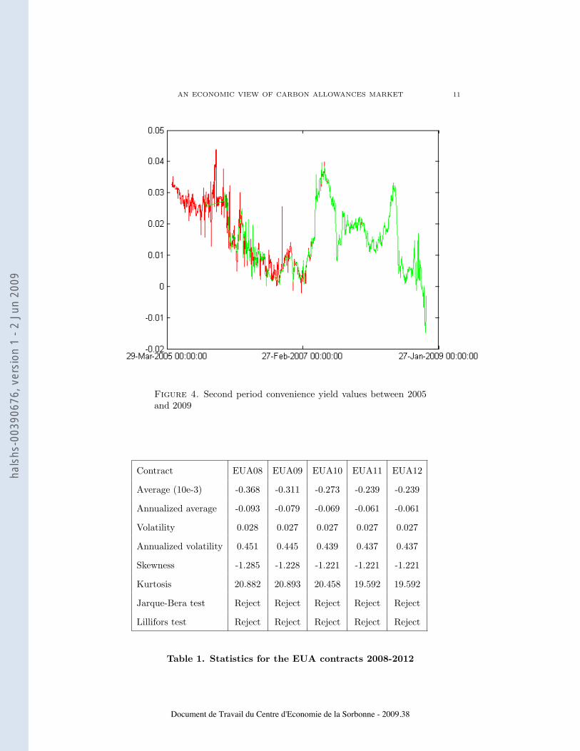
Figure 4. Second period convenience yield values between 2005and 2009
Contract EUA08 EUA09 EUA10 EUA11 EUA12
Average (10e-3) -0.368 -0.311 -0.273 -0.239 -0.239
Annualized average -0.093 -0.079 -0.069 -0.061 -0.061
Volatility 0.028 0.027 0.027 0.027 0.027
Annualized volatility 0.451 0.445 0.439 0.437 0.437
Skewness -1.285 -1.228 -1.221 -1.221 -1.221
Kurtosis 20.882 20.893 20.458 19.592 19.592
Jarque-Bera test Reject Reject Reject Reject Reject
Lillifors test Reject Reject Reject Reject Reject
Table 1. Statistics for the EUA contracts 2008-2012
Document de Travail du Centre d'Economie de la Sorbonne - 2009.38
hals
hs-0
0390
676,
ver
sion
1 -
2 Ju
n 20
09
12 MARIUS-CRISTIAN FRUNZA*, DOMINIQUE GUEGAN**
Figure 5. Distributions of EUA08 daily yields and QQ Plots
Contract CER08 CER09 CER10 CER11 CER12
Average (10e-3) -0.368 -0.311 -0.273 -0.239 -0.239
Annualized average -0.093 -0.079 -0.069 -0.061 -0.061
Volatility 0.028 0.027 0.027 0.027 0.027
Annualized volatility 0.451 0.445 0.439 0.437 0.437
Skewness -1.285 -1.228 -1.221 -1.221 -1.221
Kurtosis 20.882 20.893 20.458 19.592 19.592
Jarque-Bera test Reject Reject Reject Reject Reject
Lillifors test Reject Reject Reject Reject Reject
Table 2. Statistics for the CER contracts 2008-2012
Document de Travail du Centre d'Economie de la Sorbonne - 2009.38
hals
hs-0
0390
676,
ver
sion
1 -
2 Ju
n 20
09

AN ECONOMIC VIEW OF CARBON ALLOWANCES MARKET 13
3. Model calibration and analysis
The aim of the work developed in this section is not to find the ”true” model that
would explain the behavior of the carbon market but to propose a benchmark of
different models usually used to describe the financial assets. Based on the historical
time series we calibrate some models from the classical Brownian diffusion to more
sophisticated models based on generalized hyperbolic distributions. We use the
maximum likelihood as the main criteria to discriminate the fitness of the different
models.
3.1. Classic commodities models. In this subsection we search for a model
based on Gaussian yield distribution that could fit to CO2 prices behavior. We test
different hypothesis like mean reversion and jumps in order to find the factors that
could explain the information contained by the historical time series.
3.1.1. Brownian diffusion. A Geometric Brownian Motion (GBM) or Generalized
Wiener Process (GWP) is a continuous-time stochastic process in which the log-
arithm of the randomly varying quantity follows a Brownian motion. This model
quarantines that prices levels are always positive. In this model proportional
changes in the asset prices, denoted by S, are assumed to have constant instan-
taneous drift µ, and volatility σ. The mathematical description of this property is
given by the following stochastic differential equation:
(3.1.1)dS
S= µ · dt+ σ · dB.
Here dS represents the increment in the asset price process during a small interval
of time dt, and dB is the underlying uncertainly driving the model and represents
an increment in a Wiener process during dt. Under the transformation x = ln(S)
and using Ito’s lemma we obtain the following process for the natural logarithm of
the spot prices:
Document de Travail du Centre d'Economie de la Sorbonne - 2009.38
hals
hs-0
0390
676,
ver
sion
1 -
2 Ju
n 20
09
14 MARIUS-CRISTIAN FRUNZA*, DOMINIQUE GUEGAN**
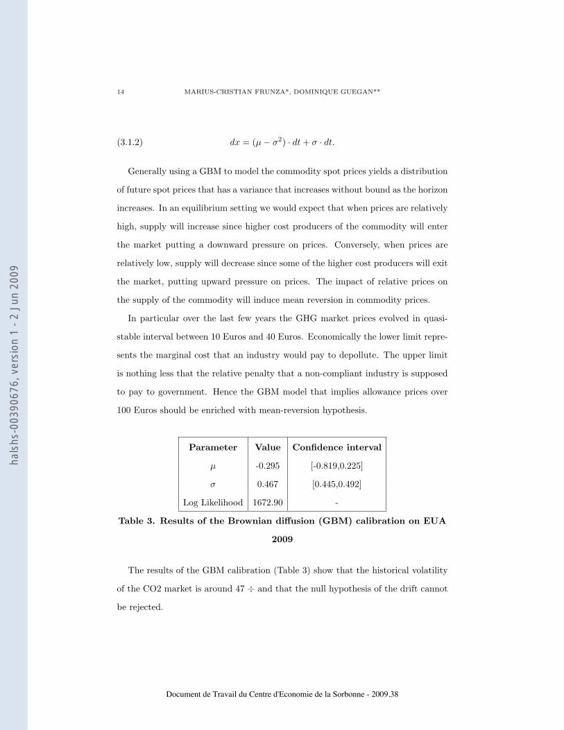
(3.1.2) dx = (µ− σ2) · dt+ σ · dt.
Generally using a GBM to model the commodity spot prices yields a distribution
of future spot prices that has a variance that increases without bound as the horizon
increases. In an equilibrium setting we would expect that when prices are relatively
high, supply will increase since higher cost producers of the commodity will enter
the market putting a downward pressure on prices. Conversely, when prices are
relatively low, supply will decrease since some of the higher cost producers will exit
the market, putting upward pressure on prices. The impact of relative prices on
the supply of the commodity will induce mean reversion in commodity prices.
In particular over the last few years the GHG market prices evolved in quasi-
stable interval between 10 Euros and 40 Euros. Economically the lower limit repre-
sents the marginal cost that an industry would pay to depollute. The upper limit
is nothing less that the relative penalty that a non-compliant industry is supposed
to pay to government. Hence the GBM model that implies allowance prices over
100 Euros should be enriched with mean-reversion hypothesis.
Parameter Value Confidence interval
µ -0.295 [-0.819,0.225]
σ 0.467 [0.445,0.492]
Log Likelihood 1672.90 -
Table 3. Results of the Brownian diffusion (GBM) calibration on EUA
2009
The results of the GBM calibration (Table 3) show that the historical volatility
of the CO2 market is around 47 ÷ and that the null hypothesis of the drift cannot
be rejected.
Document de Travail du Centre d'Economie de la Sorbonne - 2009.38
hals
hs-0
0390
676,
ver
sion
1 -
2 Ju
n 20
09

AN ECONOMIC VIEW OF CARBON ALLOWANCES MARKET 15
3.1.2. Mean reverse Brownian diffusion. The mean-reverting stochastic behavior
(GBMMR) of commodity spot prices can be well understood by looking at the one
factor model developed by Schwartz [9] and developed for energy prices by Knittel
[12] given by the following equation:
(3.1.3)dS
S= α · (ln(S)−m) · dt+ σ · dB.
In this model the spot price mean reverts to the long-term level S = exp(µ) at a
speed given by the mean reversion rate, α, σ > 0. The meaning of mean reversion
can be understood by looking at the first term of the equation (3.1.3). If the spot
price S is above the long-term level S then the drift of the spot price will be nega-
tive and the price will tend to revert back towards the long-term level. Similarly,
if the spot price is below the long-term level then the drift will be positive and the
price will tend to move back towards the long-term level as the random change in
the spot price may be of the opposite sign and greater in magnitude than the drift
component.
Defining x = lnS and applying Ito’s Lemma in equation (3.1.3), the natural
logarithm of the spot price can be characterized by an Ornstein-Uhlenbeck (OU)
stochastic process:
(3.1.4) dx = (m− x) · dt+ ς · dB,
where m = µ -σ2/2α, ς > 0. The speed of mean reversion, α>0, measures the
degree of mean reversion to the long term mean log price m. The dynamics of the
OU process under the equivalent martingale measure can be written as:
(3.1.5) dx = (m∗ − x) · dt+ ς · dB∗.
Document de Travail du Centre d'Economie de la Sorbonne - 2009.38
hals
hs-0
0390
676,
ver
sion
1 -
2 Ju
n 20
09
16 MARIUS-CRISTIAN FRUNZA*, DOMINIQUE GUEGAN**
where m* = m - λ and λ is the market price of risk. The market price of risk can
be calculated by taking into account futures term structure of the commodity. For
further considerations, market price of risk will be assumed zero. By integrating
equation (3.1.5) we get an expression for the logarithm of future spot prices:
(3.1.6) x(t) = m∗ · (1− e−α(t−t0) + x(t0)e−α(t−t0)) + σe−α(t) ·∫e−α(u)dB∗(u),
where t0 represents the initial moment of the diffusion. In a discrete version the
above equation becomes approximatively as follows:
(3.1.7) xt = c+ β · xt−1 + εt,
where c = m∗(1− e−α), β = e−α, and εt = σ ·∫eα(u−t)dB∗(u).
The error term (εt)t is a Gaussian white noise with variance σε2 equal to σ2(1−
e−2α)/2α. In other words the conditional distribution of xt | xt−1 is given by the
following expression:
(3.1.8) xt|xt−1 ∼ N(c+ β · xt−1, σ2ε ),
and N denotes the Gaussian law.
Document de Travail du Centre d'Economie de la Sorbonne - 2009.38
hals
hs-0
0390
676,
ver
sion
1 -
2 Ju
n 20
09
AN ECONOMIC VIEW OF CARBON ALLOWANCES MARKET 17
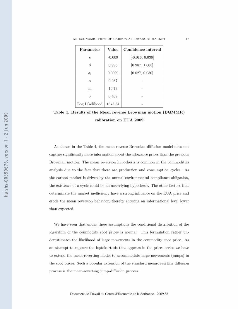
Parameter Value Confidence interval
c -0.009 [-0.016, 0.036]
β 0.996 [0.987, 1.005]
σt 0.0029 [0.027, 0.030]
α 0.937 -
m 16.73 -
σ 0.468 -
Log Likelihood 1673.84 -
Table 4. Results of the Mean reverse Brownian motion (BGMMR)
calibration on EUA 2009
As shown in the Table 4, the mean reverse Brownian diffusion model does not
capture significantly more information about the allowance prices than the previous
Brownian motion. The mean reversion hypothesis is common in the commodities
analysis due to the fact that there are production and consumption cycles. As
the carbon market is driven by the annual environmental compliance obligation,
the existence of a cycle could be an underlying hypothesis. The other factors that
determinate the market inefficiency have a strong influence on the EUA price and
erode the mean reversion behavior, thereby showing an informational level lower
than expected.
We have seen that under these assumptions the conditional distribution of the
logarithm of the commodity spot prices is normal. This formulation rather un-
derestimates the likelihood of large movements in the commodity spot price. As
an attempt to capture the leptokurtosis that appears in the prices series we have
to extend the mean-reverting model to accommodate large movements (jumps) in
the spot prices. Such a popular extension of the standard mean-reverting diffusion
process is the mean-reverting jump-diffusion process.
Document de Travail du Centre d'Economie de la Sorbonne - 2009.38
hals
hs-0
0390
676,
ver
sion
1 -
2 Ju
n 20
09

18 MARIUS-CRISTIAN FRUNZA*, DOMINIQUE GUEGAN**
3.1.3. Jump diffusion - Gaussian Mixture. Before exploring the mean-reverting
jump-diffusion process we will make a turnaround to the switching regime mod-
els, like an overture to the jumps models. A special case of the regime switching
models is the Gaussian mixture - Gaussian movement with jumps (GBMJ) distribu-
tions [10]. Let the state (regime) that an unobserved process is, at time t, be noted
as st, where there are m possible regimes (st = 1, 2,... , m). When the unobserved
process is at the state j, i.e. st=j, the observed sample xt is presumed to have been
drawn from a N(µj ;σ2j) distribution. Hence, the density of xt conditional on the
state variable st taking on the value j is
(3.1.9) f(xt/st = j; θ) =1√
2πσj· e−
(xt−µj)2
2σj2
,
for j = 1, 2,...,m. Here θ is a vector of parameters that includes µ1,µ2 ... , µm and
σ12,σ2
2 ... , σm2. The unobserved regime st is presumed to have been generated
by some probability distribution, for which the unconditional probability that st
takes on the value j is πj defined as P(st = j;θ)=πj for j = 1, 2,... m.
The unconditional density of xt can be found by summing over all possible values
that the state variable can take on:
(3.1.10) f(xt; θ) =m∑j=1
P (xt, st = j; θ) =m∑j=1
πj√2πσj
· e−
(xt−µj)2
2σj2
.
For example for a Mixture of two Gaussian distributions the unconditional den-
sity is :
(3.1.11) f(xt; θ) =π1√2πσ1
· e−(xt−µ1)2
2σ12 +π2√2πσ2
· e−(xt−µ2)2
2σ22 .
Since the regime st is unobserved, the expression by equation (3.1.11) is the
relevant density describing the actually observed data (xt). If the state variable st
is distributed across different times t, then the log likelihood for the observed data
can be calculated from equation (3.1.11) as
Document de Travail du Centre d'Economie de la Sorbonne - 2009.38
hals
hs-0
0390
676,
ver
sion
1 -
2 Ju
n 20
09
AN ECONOMIC VIEW OF CARBON ALLOWANCES MARKET 19
(3.1.12) L(θ) =m∑t=1
logf(xt; θ).
The maximum likelihood estimate of θ is obtained by maximizing the expression
(3.1.12) subject to constrains that π1 + π2 + ... + πm = 1 and πj ≥ 0 for j = 1,
2,...,m. One way this can be achieved using numerical procedures or using the
Expectation-Maximization algorithm developed by Dempster [7].
If jumps in prices correspond to the arrival of ”abnormal” information, the num-
ber of such information arrivals ought not to be very large. For practical considera-
tions, if t corresponds to one trading day, no more than one ”abnormal” information
arrival is to be expected on average. Furthermore, if returns were computed for
finer time intervals, the Bernoulli model would converge to the Poisson model.
(3.1.13)dS
S= µ · dt+ σ · dB + κ · dQ.
At each time period if we do not have an arrival of abnormal information (event
with probability (1-λ)) the next logprice is drawn by a conditional normal dis-
tribution with mean µ and variance σ2. If we do have an arrival of ”abnormal”
information, a jump occurs and the log-price is drawn from a conditional normal
distribution with mean µ + µκ and variance σ2 + σ2κ. Hence a Bernoulli jump-
diffusion process can be written as a Gaussian mixture:
(3.1.14) xt ∼ (1− λ) ·N(µ, σ2) + λ ·N(µκ, σ2κ),
where µκ is average size of a jump and σ2κ is the variance of the jumps.
Document de Travail du Centre d'Economie de la Sorbonne - 2009.38
hals
hs-0
0390
676,
ver
sion
1 -
2 Ju
n 20
09
20 MARIUS-CRISTIAN FRUNZA*, DOMINIQUE GUEGAN**
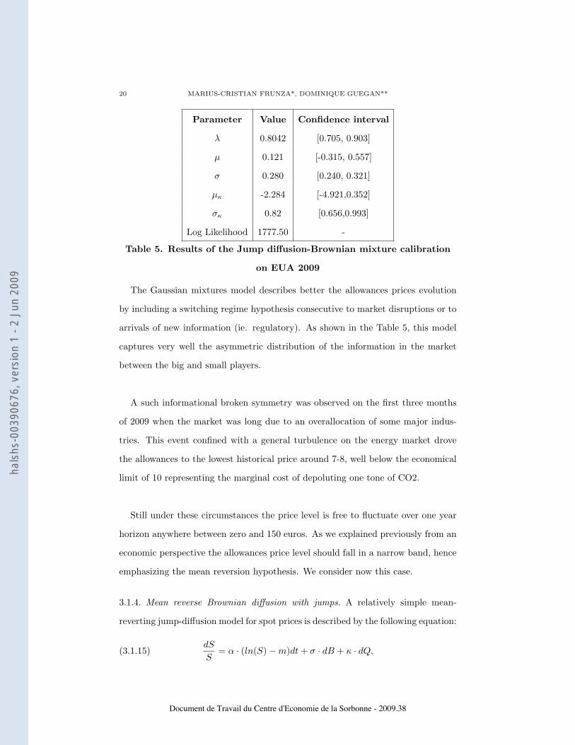
Parameter Value Confidence interval
λ 0.8042 [0.705, 0.903]
µ 0.121 [-0.315, 0.557]
σ 0.280 [0.240, 0.321]
µκ -2.284 [-4.921,0.352]
σκ 0.82 [0.656,0.993]
Log Likelihood 1777.50 -
Table 5. Results of the Jump diffusion-Brownian mixture calibration
on EUA 2009
The Gaussian mixtures model describes better the allowances prices evolution
by including a switching regime hypothesis consecutive to market disruptions or to
arrivals of new information (ie. regulatory). As shown in the Table 5, this model
captures very well the asymmetric distribution of the information in the market
between the big and small players.
A such informational broken symmetry was observed on the first three months
of 2009 when the market was long due to an overallocation of some major indus-
tries. This event confined with a general turbulence on the energy market drove
the allowances to the lowest historical price around 7-8, well below the economical
limit of 10 representing the marginal cost of depoluting one tone of CO2.
Still under these circumstances the price level is free to fluctuate over one year
horizon anywhere between zero and 150 euros. As we explained previously from an
economic perspective the allowances price level should fall in a narrow band, hence
emphasizing the mean reversion hypothesis. We consider now this case.
3.1.4. Mean reverse Brownian diffusion with jumps. A relatively simple mean-
reverting jump-diffusion model for spot prices is described by the following equation:
(3.1.15)dS
S= α · (ln(S)−m)dt+ σ · dB + κ · dQ,
Document de Travail du Centre d'Economie de la Sorbonne - 2009.38
hals
hs-0
0390
676,
ver
sion
1 -
2 Ju
n 20
09
AN ECONOMIC VIEW OF CARBON ALLOWANCES MARKET 21
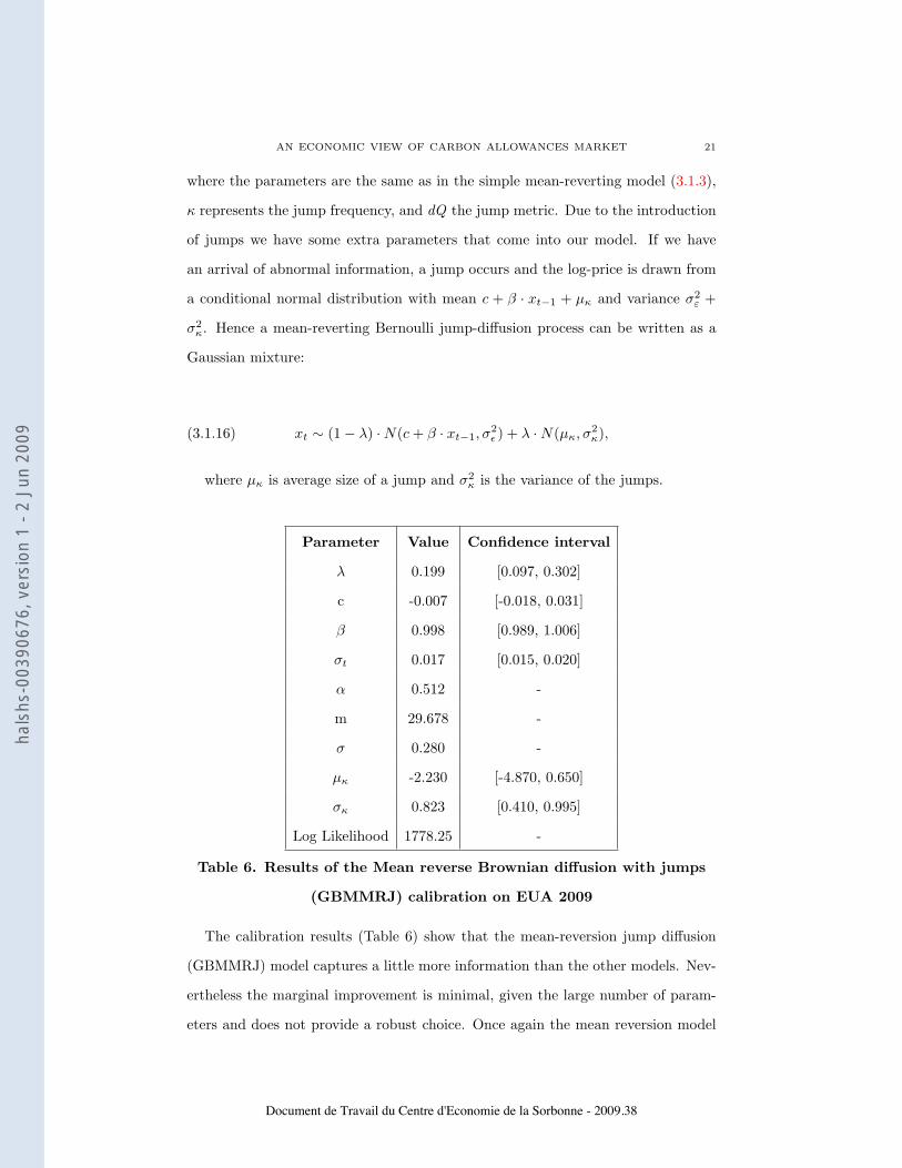
where the parameters are the same as in the simple mean-reverting model (3.1.3),
κ represents the jump frequency, and dQ the jump metric. Due to the introduction
of jumps we have some extra parameters that come into our model. If we have
an arrival of abnormal information, a jump occurs and the log-price is drawn from
a conditional normal distribution with mean c + β · xt−1 + µκ and variance σ2ε +
σ2κ. Hence a mean-reverting Bernoulli jump-diffusion process can be written as a
Gaussian mixture:
(3.1.16) xt ∼ (1− λ) ·N(c+ β · xt−1, σ2ε ) + λ ·N(µκ, σ2
κ),
where µκ is average size of a jump and σ2κ is the variance of the jumps.
Parameter Value Confidence interval
λ 0.199 [0.097, 0.302]
c -0.007 [-0.018, 0.031]
β 0.998 [0.989, 1.006]
σt 0.017 [0.015, 0.020]
α 0.512 -
m 29.678 -
σ 0.280 -
µκ -2.230 [-4.870, 0.650]
σκ 0.823 [0.410, 0.995]
Log Likelihood 1778.25 -
Table 6. Results of the Mean reverse Brownian diffusion with jumps
(GBMMRJ) calibration on EUA 2009
The calibration results (Table 6) show that the mean-reversion jump diffusion
(GBMMRJ) model captures a little more information than the other models. Nev-
ertheless the marginal improvement is minimal, given the large number of param-
eters and does not provide a robust choice. Once again the mean reversion model
Document de Travail du Centre d'Economie de la Sorbonne - 2009.38
hals
hs-0
0390
676,
ver
sion
1 -
2 Ju
n 20
09

22 MARIUS-CRISTIAN FRUNZA*, DOMINIQUE GUEGAN**
does not capture the suitable information. As a heavy tendency of the classic mod-
els calibration we underline the necessity of considering the jumps as an accurate
approximation of markets regime variations.
3.2. Generalized Hyperbolic models. Mandelbrot was the first that challenged
the idea that the Gaussian behavior of financial yields in the early 50’s. His sug-
gestion that the normal distribution is to ”gentle” regarding the extreme events
was fully proved by the past financial downturns as well as the actual crisis. More
by challenging the normality of the yields we touch indirectly to the validity of
the EMH. As the carbon market is characterized by a lack of transparency and
by a quasi-regulated status it is obvious that the completeness of the information
contained in the market price is relative. Even if the classic commodities models
seem to give sufficient results, from the conceptual perspective it is necessary to
challenge the normality of the carbon assets yields and to search for other classes
of distributions that give more priority to extreme events.
As some recent research of Eberlein and Prause [8], Brandorff-Nielsen [3] showed
the distributions of many financial quantities are well-known to have heavy tails,
exhibit skewness, and have other non-Gaussian characteristics. The empirical dis-
tribution of daily returns from financial market variables such as exchange rates,
equity prices, and interest rates, is often skewed, having one heavy, and one semi-
heavy, or more Gaussian-like tail.
In this section we will make a quick review of the generalized hyperbolic functions
and focus on the Normal Inverse Gaussian, one of the more used. Then we will
compare the fitness of the NIG with that of the other members of this family and
with the classic models. We will also add the mean reversion hypothesis into a
discrete form.
As quoted in a lot of works in the literature [17], the generic form of a generalized
hyperbolic model is given by :
Document de Travail du Centre d'Economie de la Sorbonne - 2009.38
hals
hs-0
0390
676,
ver
sion
1 -
2 Ju
n 20
09
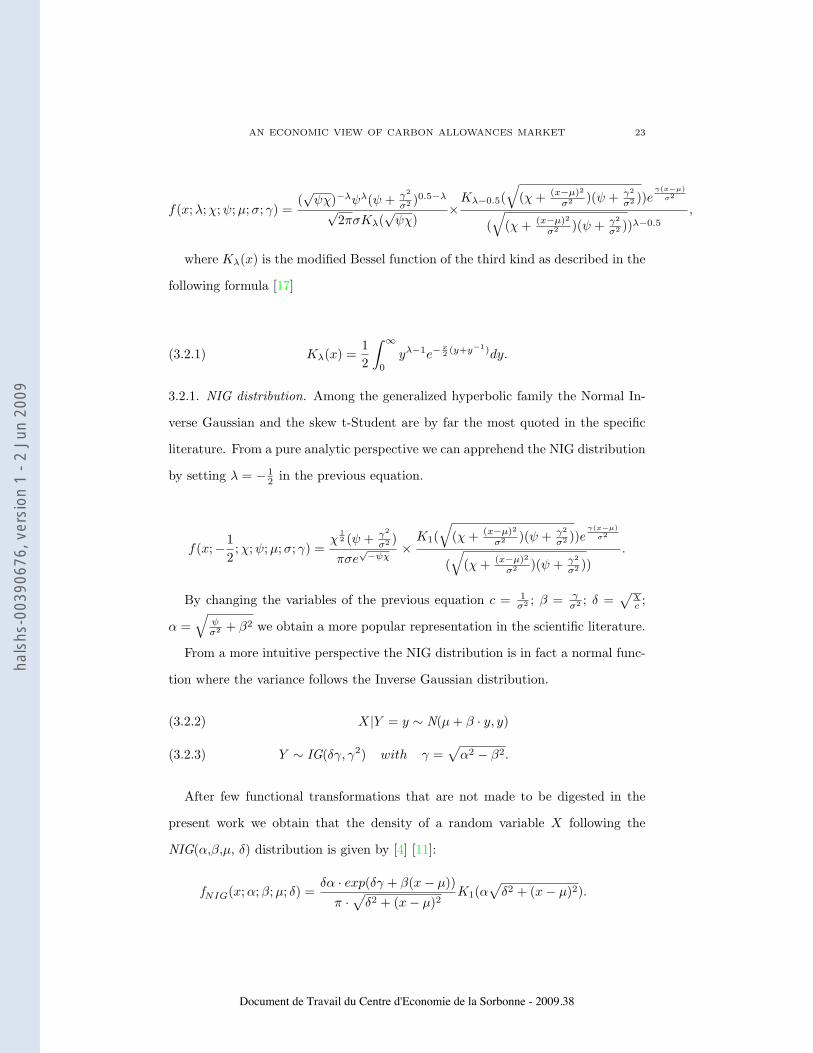
AN ECONOMIC VIEW OF CARBON ALLOWANCES MARKET 23
f(x;λ;χ;ψ;µ;σ; γ) =(√ψχ)−λψλ(ψ + γ2
σ2 )0.5−λ√
2πσKλ(√ψχ)
×Kλ−0.5(
√(χ+ (x−µ)2
σ2 )(ψ + γ2
σ2 ))eγ(x−µ)
σ2
(√
(χ+ (x−µ)2
σ2 )(ψ + γ2
σ2 ))λ−0.5
,
where Kλ(x) is the modified Bessel function of the third kind as described in the
following formula [17]
(3.2.1) Kλ(x) =12
∫ ∞
0
yλ−1e−x2 (y+y−1)dy.
3.2.1. NIG distribution. Among the generalized hyperbolic family the Normal In-
verse Gaussian and the skew t-Student are by far the most quoted in the specific
literature. From a pure analytic perspective we can apprehend the NIG distribution
by setting λ = − 12 in the previous equation.
f(x;−12;χ;ψ;µ;σ; γ) =
χ12 (ψ + γ2
σ2 )πσe
√−ψχ
×K1(
√(χ+ (x−µ)2
σ2 )(ψ + γ2
σ2 ))eγ(x−µ)
σ2
(√
(χ+ (x−µ)2
σ2 )(ψ + γ2
σ2 )).
By changing the variables of the previous equation c = 1σ2 ; β = γ
σ2 ; δ =√
χc ;
α =√
ψσ2 + β2 we obtain a more popular representation in the scientific literature.
From a more intuitive perspective the NIG distribution is in fact a normal func-
tion where the variance follows the Inverse Gaussian distribution.
X|Y = y ∼ N(µ+ β · y, y)(3.2.2)
Y ∼ IG(δγ, γ2) with γ =√α2 − β2.(3.2.3)
After few functional transformations that are not made to be digested in the
present work we obtain that the density of a random variable X following the
NIG(α,β,µ, δ) distribution is given by [4] [11]:
fNIG(x;α;β;µ; δ) =δα · exp(δγ + β(x− µ))π ·
√δ2 + (x− µ)2
K1(α√δ2 + (x− µ)2).
Document de Travail du Centre d'Economie de la Sorbonne - 2009.38
hals
hs-0
0390
676,
ver
sion
1 -
2 Ju
n 20
09
24 MARIUS-CRISTIAN FRUNZA*, DOMINIQUE GUEGAN**
Hence it is obvious that the Normal Inverse Gaussian distribution is a mixture of
normal and inverse Gaussian distributions.
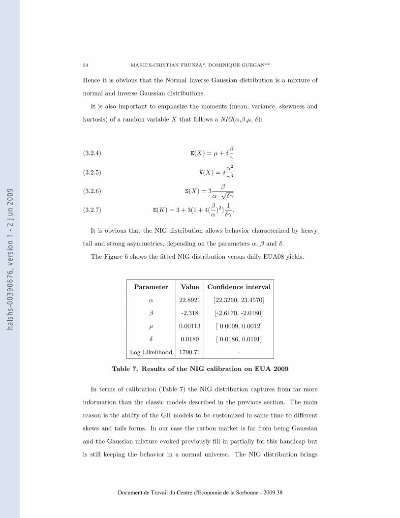
It is also important to emphasize the moments (mean, variance, skewness and
kurtosis) of a random variable X that follows a NIG(α,β,µ, δ):
E(X) = µ+ δβ
γ(3.2.4)
V(X) = δα2
γ3(3.2.5)
S(X) = 3β
α ·√δγ
(3.2.6)
E(K) = 3 + 3(1 + 4(β
α)2)
1δγ.(3.2.7)
It is obvious that the NIG distribution allows behavior characterized by heavy
tail and strong asymmetries, depending on the parameters α, β and δ.
The Figure 6 shows the fitted NIG distribution versus daily EUA08 yields.
Parameter Value Confidence interval
α 22.8921 [22.3260, 23.4570]
β -2.318 [-2.6170, -2.0180]
µ 0.00113 [ 0.0009, 0.0012]
δ 0.0189 [ 0.0186, 0.0191]
Log Likelihood 1790.71 -
Table 7. Results of the NIG calibration on EUA 2009
In terms of calibration (Table 7) the NIG distribution captures from far more
information than the classic models described in the previous section. The main
reason is the ability of the GH models to be customized in same time to different
skews and tails forms. In our case the carbon market is far from being Gaussian
and the Gaussian mixture evoked previously fill in partially for this handicap but
is still keeping the behavior in a normal universe. The NIG distribution brings
Document de Travail du Centre d'Economie de la Sorbonne - 2009.38
hals
hs-0
0390
676,
ver
sion
1 -
2 Ju
n 20
09

AN ECONOMIC VIEW OF CARBON ALLOWANCES MARKET 25
Figure 6. NIG Distribution adapted on EUA08: on the left yieldshistogram and the fitted NIG; on the right QQ plot.
another dimension with more parameters that are less intuitive than the Brownian
process, but that are more suitable to asymmetric distributions with fat tails.
3.2.2. Other GH distributions. Even if the NIG and the Skew-t Student distribu-
tions are the most reputed amongst the generalized hyperbolic family, a righteous
approach would be to scan for the distribution that captures the highest level of
information offered by the times series. By changing λ from -0.5 to other values we
could search for the distribution providing the best fit. This topic will constitute
the focus of a future work.
3.2.3. NIG - Gaussian mixture. As we already saw in the previous section the
Gaussian mixture hypothesis captures a lot of information concerning carbon prices
behavior. Beside the historical series the economical facts show as that the carbon
prices fluctuates, this conducts us to intricate the heavy tail asymmetric behavior
with the classic Gaussian hypothesis, and we consider the following model:
Document de Travail du Centre d'Economie de la Sorbonne - 2009.38
hals
hs-0
0390
676,
ver
sion
1 -
2 Ju
n 20
09
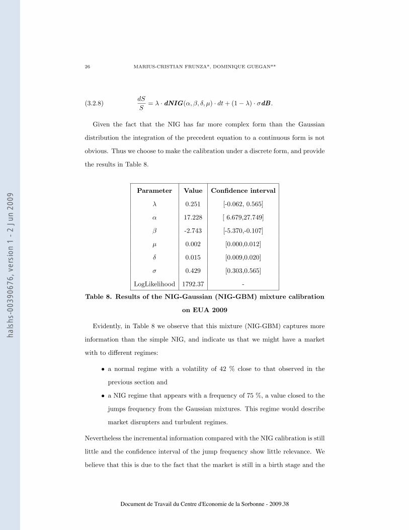
26 MARIUS-CRISTIAN FRUNZA*, DOMINIQUE GUEGAN**
(3.2.8)dS
S= λ · dNIG(α, β, δ, µ) · dt+ (1− λ) · σdB .
Given the fact that the NIG has far more complex form than the Gaussian
distribution the integration of the precedent equation to a continuous form is not
obvious. Thus we choose to make the calibration under a discrete form, and provide
the results in Table 8.
Parameter Value Confidence interval
λ 0.251 [-0.062, 0.565]
α 17.228 [ 6.679,27.749]
β -2.743 [-5.370,-0.107]
µ 0.002 [0.000,0.012]
δ 0.015 [0.009,0.020]
σ 0.429 [0.303,0.565]
LogLikelihood 1792.37 -
Table 8. Results of the NIG-Gaussian (NIG-GBM) mixture calibration
on EUA 2009
Evidently, in Table 8 we observe that this mixture (NIG-GBM) captures more
information than the simple NIG, and indicate us that we might have a market
with to different regimes:
• a normal regime with a volatility of 42 % close to that observed in the
previous section and
• a NIG regime that appears with a frequency of 75 %, a value closed to the
jumps frequency from the Gaussian mixtures. This regime would describe
market disrupters and turbulent regimes.
Nevertheless the incremental information compared with the NIG calibration is still
little and the confidence interval of the jump frequency show little relevance. We
believe that this is due to the fact that the market is still in a birth stage and the
Document de Travail du Centre d'Economie de la Sorbonne - 2009.38
hals
hs-0
0390
676,
ver
sion
1 -
2 Ju
n 20
09
AN ECONOMIC VIEW OF CARBON ALLOWANCES MARKET 27
pattern of behavior are not yet very accentuated.
The bottom line of this part is that carbon allowances need both four moments
distributions and broken symmetry regimes in order to capture more of its behavior.
Future developments would include switching regimes with generalized hyperbolic
distributions and autoregressive volatility behavior.
4. Application to risk modeling of a CO2 derivative
At the dawn of the carbon market a wide range of specific financial products
aroused in order to answer to the different needs and to profit from arbitrage op-
portunities. From forward contracts to exotic options and structured products the
financial institutions cover all the spectrum of derivatives mainly by leveraging on
their commodities market experience.
Amongst those products, one of the most popular is the EUA-CER arbitrage
swap, a CO2 structured strategy developed by most of the financial institutions
in the carbon finance. This product allows to generate riskless income, by taking
the price difference between CER and EUA prices. It is important to mention
that under the European Environmental Compliance directives a company can be
compliant if owns the necessary amount of allowances. Nevertheless it is also allowed
to own Kyoto credits (CER) instead of EUA in order to be compliant at a level
between 10 and 20÷ depending on the local regulation.
4.1. The Arbitrage Swap. The difference between prices of the EUA and CER
can vary over time. The carbon arbitrage swap creates profitability from the
immobilized allowances and income from the prices difference between EUA and
CER without any consequences associated with the price fluctuation. The figure 7
presents the flows generated by the product.
The carbon arbitrage swap can be adapted for time horizons between one and
five years 2008-2012, until the end of the second Kyoto period. It is tailored in such
Document de Travail du Centre d'Economie de la Sorbonne - 2009.38
hals
hs-0
0390
676,
ver
sion
1 -
2 Ju
n 20
09

28 MARIUS-CRISTIAN FRUNZA*, DOMINIQUE GUEGAN**
Figure 7. Carbon Arbitrage product
manner that the client is compliant at each regulatory deadline. Hence the client
receives the credits each year before its compliance date.
At the beginning of the transaction the industrial company delivers to the broker
the quotas that are cashed out via a financial institution (credit company) on
the market. In the same time the broker locks by an agreement with the credit
company, the prices for the futures deliveries of the credits. In the following years
the credit company will deliver periodically before the equivalent credits for the
received quotas.
For example let us consider an industrial company with a CER limitation of 10÷
and suppose that the company has 1 million allocated 2008 quotas. The industry
can thus surrender 100,000 CERs per year. Over 5 years therefore it has recourse
to 500,000 CERs. In March 2008 the company transfers 500,000 of the 1 millon
Document de Travail du Centre d'Economie de la Sorbonne - 2009.38
hals
hs-0
0390
676,
ver
sion
1 -
2 Ju
n 20
09
AN ECONOMIC VIEW OF CARBON ALLOWANCES MARKET 29
EUAs which it receives from the Commission into CERs. Since the CER trades
at a lower price than the EUA, the difference in price in the exchange releases a
premium. This difference in price fluctuates today between 4 and 5,5 euros. In our
example, the premium would be fixed for example at 4 euros per ton of CO2 given
up for conversion. The customer will receive 500,000 * 4 = 2 million Euros at the
date of the signature of the contract. The delivery of the EUA between the broker
and the industry can be done immediately.
4.2. Economical capital allocated to an Arbitrage Swap product. It is
obvious that the financial counterparty could be under default any time between
the date of the contract and the effective deliveries dates of the CERs. In this case
the broker must replace the CER, by buying them at the market price. Under a
scenario of a rising trend of CERs, the broker should fill the difference between
the negotiated price at the beginning of the contract and the market price at the
moment of default.
In the new heavy regulated environment each financial establishment should
have enough capital to cover the extreme risk undertaken by its operations. In
our case the broker should have put aside enough economical capital to cover the
consequences of a probable default of the financial counterparty. A classic metric of
the economical capital used by many financial institutions for a structured product
is the value at risk (VaR). The VaR is a very intuitive measure but has some
obvious failures as it shows no subaditivity (the value of the risk measure for two
risks combined will not be greater than for the risks treated separately). Some
remedy proposal are discussed by Artzner[1] that will not be applied in this paper
in order to keep a basic metric and to compare only the adequacy of the underlying
model. Mathematically, VaR is defined as follows, for α given:
(4.2.1) V aRα(X) = −inf(x | P[X ≤ x > α]).
Document de Travail du Centre d'Economie de la Sorbonne - 2009.38
hals
hs-0
0390
676,
ver
sion
1 -
2 Ju
n 20
09

30 MARIUS-CRISTIAN FRUNZA*, DOMINIQUE GUEGAN**
The risk undertaken by the broker is the difference between the negotiated credit
price and the observed price in case of a default of the credit company. Hence in
order to evaluate the Value at Risk of the product three problems arise:
• estimate the default risk over the product time horizon ;
• estimate the spread behavior between the EUA and CER ;
• cumulate the credit and the market risks.
The default risk is estimated via the default probabilities and transition matrices
given by the rating agencies. The behavior of the EUA - CER spread deserves a
more detailed analysis and will not constitute the object of the present paper. We
will model the spread by a fixed discount rate to the EUA prices. We will provide
the analysis in a future work. The imbrication of both credit and market risk
is made via a CreditMetrics-like approach. Otherwise we simulate the exposure
scenarios in case of counterparty default, thereby obtaining the aggregated risk
distribution.
As we mentioned previously the product exposure in case of default is the spread
between the CER price at the default moment and the price at the moment of the
deal on upward market. The following equation is nothing else but the price of an
European call with a strike equivalent to the initial price of the CER.
(4.2.2) Exposure(t) = E(max(0, (SCER(t)− SCER(0)) · e−r·t),
where r is the free risk rate and SCER(t) and SCER(0) are the CER prices at the
moments t and 0;
Our approach to obtain the loss distribution consists in simulating via a Monte
Carlo method a grand number of events with two potential consequences:
• No default observed and no loss occurred
• Default of the financial counterparty and an estimated loss as the average
of the positive spreads between the future CER prices and the initial CER
price,
Document de Travail du Centre d'Economie de la Sorbonne - 2009.38
hals
hs-0
0390
676,
ver
sion
1 -
2 Ju
n 20
09
AN ECONOMIC VIEW OF CARBON ALLOWANCES MARKET 31
then,
(4.2.3) Loss(t) = [Zeros[NS·(1−PD(t))], Exposure(t)[NS·PD(t)]],
where Zeros[NS·(1−PD(t))] is a vector containing zeros with a length of NS · (1 −
PD(t)), Loss(t) is the simulated vector of potential losses, and PD(t) is the default
probability at the moment t.
As we show, at a certain horizon t, the simulated loss vector is the result of the
concatenation of a zero vector for cases of non-default and of the exposure vector
for the default cases. In the environment of investment banking, the VaR measure
is considered for a 10 working days horizon and at a 95% confidence level. This
kind of risk metric is adapted for marketable and liquid securities, but once we
enter in the area of structured products with long horizon and low liquidity, it is
suitable to consider a VaR time horizon close to that of the product.
The classic view of risk universe is under a normal metric and a risk-neutral
probability adapted for the efficient markets. In our case we considered a Monte
Carlo VaR based on non-Gaussian distributions calibrated on the historical times
series. We emphasize, in the next subsection, the main difference between the
various models taken in account.
4.3. Value at Risk: Classic versus GH models. In the following, we compare
the economical capital figures for the carbon arbitrage swap measured via different
models calibrated in the previous sections. We apply the example given in the
previous paragraph with 1 million quotas per year, for each delivery horizon on the
product, thereby providing a Value at Risk figure for each year.
The product risk exposure depends on two factors: the nominal exposure of the
swap and the volatility of the market. It is obvious that the nominal exposure
is diminishing with the passage of time because periodic deliveries are made. On
the other hand the passage of the time amplifies the volatility of the market and
indirectly the product risk exposure. The two factors have different sensibilities
depending on the time horizon and in consequence the maximum marginal exposure
Document de Travail du Centre d'Economie de la Sorbonne - 2009.38
hals
hs-0
0390
676,
ver
sion
1 -
2 Ju
n 20
09

32 MARIUS-CRISTIAN FRUNZA*, DOMINIQUE GUEGAN**
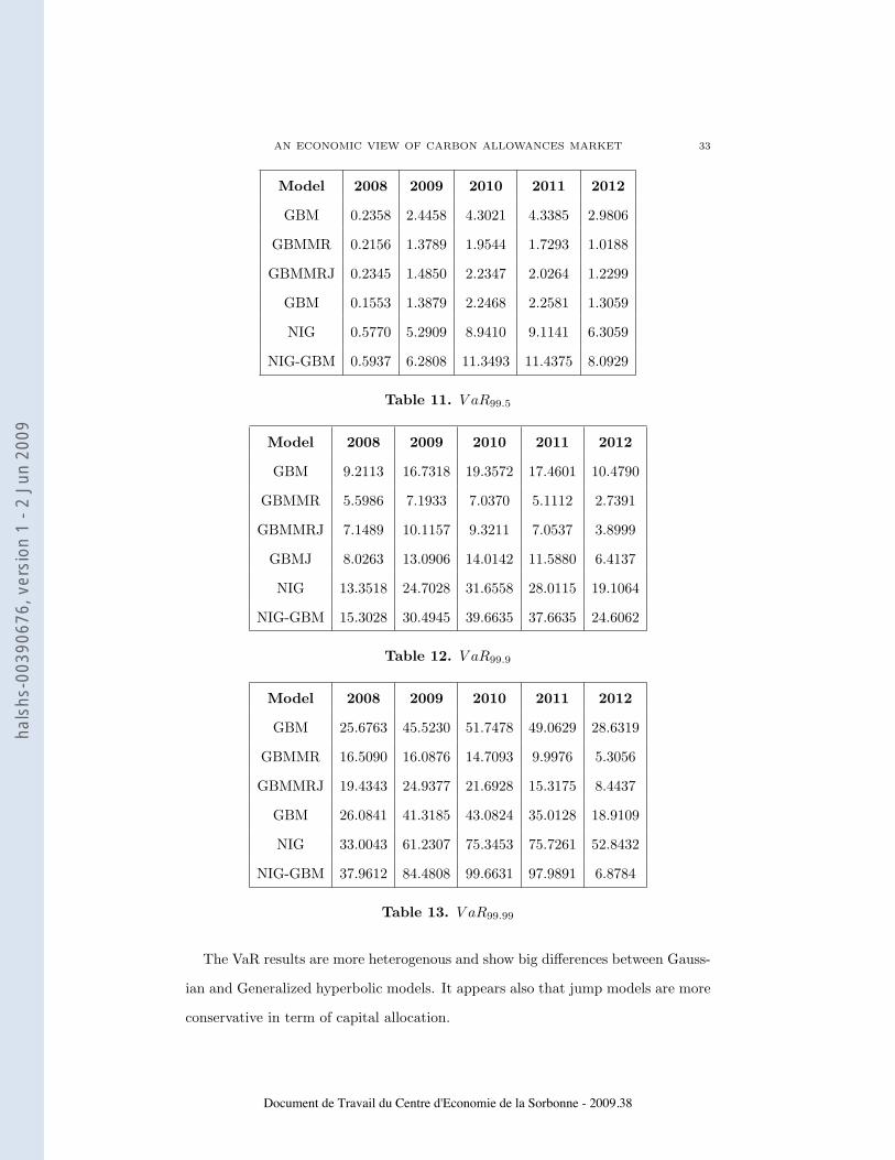
is at the half way horizon time. In table 10 we show the average loss for different
horizons and in tables 11, 12, and 13 the results of Monte Carlo VaR for α values
of 99.5%, 99.9% and 99.99%.
It appears that for a given α the VaR have heterogenous values depending of the
models. The GH and jumps models give the most conservative results due to the
fact that they contain more information about the tail behavior than the classic
models, hence emphasizing the potential extreme events.
For different values of α the variations of the risk measures are also depending
of the chosen model. Hence models with strong kurtosis tend to show bigger varia-
tions for different percentiles that classic models. This depends on the capacity of
the model to enclose significant information that could characterized the extreme
percentiles. In these cases, figures of GH and jump models consume more capital
than Brownian diffusion models.
The horizon plays an essential role for this type of product. As we have already
shown the risk horizon for the arbitrage swap is measured in years and goes far
beyond the classic ”10 days” used by the option desks. For longer horizon the VaR
becomes bigger but the incremental VaR from one year to another has a maximum
value between the second and the third year.
Model 2008 2009 2010 2011 2012
GBM 0.0148 0.0620 0.0820 0.0783 0.051
GBMMR 0.0174 0.0276 0.0315 0.0267 0.0156
GBMMRJ 0.0217 0.0362 0.0394 0.0324 0.0194
GBMJ 0.0242 0.0473 0.0554 0.0484 0.0272
NIG 0.0411 0.0991 0.1482 0.1511 0.1092
NIG-GBM 0.0461 0.1245 0.1921 0.1952 0.1402
Table 10. Average of the loss distributions
It appears that the averages of the lost distributions stay in the same range of
values for all models for a given horizon. Nevertheless the models with fat tails
show a bigger average due to the extreme losses that could appear.
Document de Travail du Centre d'Economie de la Sorbonne - 2009.38
hals
hs-0
0390
676,
ver
sion
1 -
2 Ju
n 20
09
AN ECONOMIC VIEW OF CARBON ALLOWANCES MARKET 33
Model 2008 2009 2010 2011 2012
GBM 0.2358 2.4458 4.3021 4.3385 2.9806
GBMMR 0.2156 1.3789 1.9544 1.7293 1.0188
GBMMRJ 0.2345 1.4850 2.2347 2.0264 1.2299
GBM 0.1553 1.3879 2.2468 2.2581 1.3059
NIG 0.5770 5.2909 8.9410 9.1141 6.3059
NIG-GBM 0.5937 6.2808 11.3493 11.4375 8.0929
Table 11. V aR99.5
Model 2008 2009 2010 2011 2012
GBM 9.2113 16.7318 19.3572 17.4601 10.4790
GBMMR 5.5986 7.1933 7.0370 5.1112 2.7391
GBMMRJ 7.1489 10.1157 9.3211 7.0537 3.8999
GBMJ 8.0263 13.0906 14.0142 11.5880 6.4137
NIG 13.3518 24.7028 31.6558 28.0115 19.1064
NIG-GBM 15.3028 30.4945 39.6635 37.6635 24.6062
Table 12. V aR99.9
Model 2008 2009 2010 2011 2012
GBM 25.6763 45.5230 51.7478 49.0629 28.6319
GBMMR 16.5090 16.0876 14.7093 9.9976 5.3056
GBMMRJ 19.4343 24.9377 21.6928 15.3175 8.4437
GBM 26.0841 41.3185 43.0824 35.0128 18.9109
NIG 33.0043 61.2307 75.3453 75.7261 52.8432
NIG-GBM 37.9612 84.4808 99.6631 97.9891 6.8784
Table 13. V aR99.99
The VaR results are more heterogenous and show big differences between Gauss-
ian and Generalized hyperbolic models. It appears also that jump models are more
conservative in term of capital allocation.
Document de Travail du Centre d'Economie de la Sorbonne - 2009.38
hals
hs-0
0390
676,
ver
sion
1 -
2 Ju
n 20
09
34 MARIUS-CRISTIAN FRUNZA*, DOMINIQUE GUEGAN**
5. Conclusions
Understanding the GHG market goes beyond the classic stochastic apprehension
of the financial assets like commodities and enters in a more subjective area of the
behavioral finance. Thus, the main topic of this paper is to search for an economet-
ric model that could fit the best the historical time series. The discriminant factor
to rank models relevance was the likelihood. The GHG prices show a pronounced
non-Gaussian behavior with fat tails and negative skewness. The NIG distribution
outperforms the classic Brownian models in term of quantity of information. It
appears clearly that jumps are a necessary hypothesis for an accurate modeling of
the CO2 prices.
We applied the results of the model calibration on the risk estimation of a fi-
nancial product specific to the CO2 market, the EUA -CER swap. The economical
capital allocated for carbon transaction are more conservative when we use Gener-
alized hyperbolic models than with classic Brownian models.
Further developments will include the autoregressive models [15],[14] and mem-
ory effects in the model calibration, the econometric study of the EUA - CER spread
and the macro-economical model of the CO2 market taking in account fundamental
factors.
References
1. Eber J. Heath D. Artzner P., Delbaen F., Coherent measures of risk, July 1998.
2. Truck S. Benz E., Modeling the price dynamics of co2 emission allowances, Elsevier Science
(2008).
3. O.E. Brandorff-Nielsen, Processes of normal inverse gaussian type, Finance and Stochastics
2 (1998), 41–68.
4. Liu H. Jan J.F. Chang Y.P., Hung M.C., Testing symmetry of a nig distribution, Communi-
cations in StatisticsSimulation and Computation 34 (2005), 851–862.
5. Markellos N. Daskalakis G., Are the european carbon markets efficient, Review of Futures
Markets 17 (2008), no. 2, 103–128.
6. Markellos R. Daskalakis G., Psychoyios D., Modelling co2 emission alloance prices and deriva-
tives: Evidence from european trading scheme, Journal of Banking and Finance (2009).
Document de Travail du Centre d'Economie de la Sorbonne - 2009.38
hals
hs-0
0390
676,
ver
sion
1 -
2 Ju
n 20
09
AN ECONOMIC VIEW OF CARBON ALLOWANCES MARKET 35
7. Laird N. Rubin D. Dempster, A., Maximum likelihood from incomplete data via the em algo-
rithm, Journal of the Royal Statistiacal Society 39 (1977), 1–38.
8. Prause K. Eberlein E., The generalized hyperbolic model: Fiancial derivatives and risk man-
agement, Bull. London Math. Soc. 10 (1998), 300–325.
9. Schwartz E.S., The stochastic behavior of commodity prices: Implications for valuation and
hedging, The Journal of Finance 52 (1997), no. 3, 923–973.
10. Hamilton J.D., A new approach to the economic analysis of nonstationary time series and
the business cycle, Econometrica 57 (1989), no. 2, 357–384.
11. Werner R. Kalemanova A., Schmid B., The normal inverse gaussian distribution for synthetic
cdo pricing, Risklab Germany, August 2005.
12. Roberts M. Knittel, C., An empirical examination of restructured electricity prices, Energy
Economics 27 (2005), no. 5, 791–817.
13. Taschini L. Paolella M., An econometriv analyisis of emission trading allowances, Research
papers 06-26, Swiww Finance Institute, 2006.
14. Engle R., Garch 101: The use of arch/garch models in applied econometrics, Journal of
Economic Perspectives 15 (2001), no. 4, 157–168.
15. Bollerslev T., Generalized autoregressive conditional heteroskedasticity, Journal of Economet-
rics 31 (1986), 307–327.
16. Michael Wagner Uhrig-Homburg M., Futures price dynamics of co2 emission certificates -an
empirical analysis, Tech. report, University of Karlsruhe, 2007.
17. Hu W., Calibration of multivariate generalized hyperbolic distributions using the em algo-
rithm, with applications in risk management, portfolio optimization and portfolio credit risk
Book, first ed., Florida State Univeristy, Florida, 2005.
Document de Travail du Centre d'Economie de la Sorbonne - 2009.38
hals
hs-0
0390
676,
ver
sion
1 -
2 Ju
n 20
09