1

An experimental verification of the one-dimensional

static Willis-form equations

R.W. Yao‡, H.X. Gao‡, Y.X. Sun, X.D. Yuan, Z.H. Xiang*

AML, Department of Engineering Mechanics, Tsinghua University, Beijing 100084,

China

ABSTRACT

This paper investigates the behavior of a heavy soft spring in steady circular motion.

Since the spring is inhomogeneous due to centrifugal force, one can rigorously prove

that it follows the one-dimensional static Willis-form equations. The theoretical

predictions agree very well with experimental results. It further demonstrates that

these equations can give a clear understanding of the stress-stiffening and

spin-softening effect. These findings reveal that the Willis-form equations can give

very accurate linear approximations of finite deformation problems and are also

helpful to clarify the classical concept of the principle of material frame indifference.

Keywords: Willis equations, Inhomogeneous springs, Material frame indifference,

Stress-stiffening, Spin-softening

1. Introduction

About three decades ago, Professor Willis (1981, 1997) proposed new linear

elastic equations for inhomogeneous media by using the perturbation theory. The

Willis equations include a constitutive equation * Corresponding author. Email address: xiangzhihai@tsinghua.edu.cn. ‡ These authors contributed equally to this paper.

2

eff eff σ C e S u (1a)

and an equation of motion

· eff eff σ f S e ρ u , (1b)

where σ is the stress tensor; u is the displacement vector free of rigid translations; e is

the strain tensor, / 2 e u u ; f is the body force vector; denotes the

ensemble average; the superposed dot denotes the differentiation with respect to time t;

effC , effS , effS and effρ are non-local operators acting on e , u , e and

u respectively. According to Willis (1997), the details of these operators are:

0 : : :eff xC C e C C S CC e C e , (2a)

:eff xC CS M uu , (2b)

:teff S CS e eC , (2c)

0eff t ρ u u M u , (2d)

where 0C and 0 are constant elasticity tensor and density, respectively; C and

are corresponding small perturbations; xS , xM , tS and tM are tensors

related to the Green’s function , , tG x x with the source point x and the field

point x ; and is an operator representing field integration and time-convolution. A

detailed example of is

, , , d

t

t srsM t u t

uM

x x x x x x

, (3)

where denotes the time-convolution.

In contrast to the classical linear elastic equations, the Willis equations are more

complex and abstract. Therefore, not much attention had been paid to them until the

3

upsurge of designing metamaterials with transformation methods (Shamonina and

Solymar, 2007).

In the transformation method, a wave equation in a virtual space is transformed

into a physical space through local mapping functions of independent variables

(coordinates) and dependent variables (field variables). If this equation is

form-invariant after the transformation, one can obtain the effective material

properties by comparing the corresponding terms in the original and transformed

equations. The resultant material in the physical space is called a metamaterial that is

inhomogeneous and can steer the wave front along desired trajectories. Although the

transformation method had achieved great successes in optics (Leonhardt, 2006;

Pendry et al., 2006) and acoustics (Chen and Chan, 2010), it met much difficulty in

elastics, because Milton et al. (2006) found that upon applying the local

transformation on the classical linear elastic equations in frequency domain results in

the corresponding Willis equations in local form. In another word, the classical linear

elastic equations are not form-invariant under the local transformation but the Willis

equations do.

The findings of Milton et al. (2006) aroused much interest in studying the Willis

equations. Most of these studies focused on the dynamic homogenization of

periodically inhomogeneous media (Willis, 2011; Norris et al., 2012; Srivastava and

Nemat-Nasser, 2012; Nassar et al., 2015, 2016; Torrent et al., 2015; Srivastava, 2015),

which involve non-local properties. However, if using transformation methods with

point to point mappings, one can naturally obtain local properties (Milton et al., 2006).

4

For example, Xiang (2014) proved that the form-invariance is an intrinsic character of

wave equations independent of the gauge adopted in the linear local transformation.

He also obtained the Willis equations in time domain by using the deformation

gradient as the transformation gauge for displacements:

: σ C e S u , (4a)

T· :a σ f S e K u ρ u , (4b)

where C is the symmetric elasticity tensor; ρ is the mass density tensor; and af is an

additional external body force in the physical space; T :S e means ijk ijS e .

By noticing the differential property of time convolution

d

dt , (5)

one can easily prove that the operator , as shown in Eq. (3), has the similar

property:

d

dt φ ψ φ ψ φ ψ . (6)

Thus, Eq. (1) can also be written as:

eff eff σ C e D u , (7a)

· eff eff σ f D e u uK , (7b)

where

:eff xC CD M , (8a)

:teff S C CD , (8b)

teff K M , (8c)

0 . (8d)

Eq. (7) is in the same form as that of Eq. (4), which implies that Eq. (4) is also a

5

possible result under the original theoretical framework of Willis (1997).

With the presence of pre-stresses 0σ , Xiang and Yao (2016) further proved that

the S in Eq. (4) is the gradient of 0σ and K u equals to the increment of the

body force due to the change of the small perturbation from the pre-stressed

configuration to the current configuration. They also pointed out that these equations

are still valid for static problems if the inertia is ignored, namely,

0: σ e σC u , (9a)

T0· :a σ f eσ K u , (9b)

where T0 :σ e means 0,ij k kje . Milton et al. (2006) also realized that if the

microstructure in homogenization is sufficiently small, then these non-local effective

operators in Eq. (1) might be approximated to local operators. In this sense, Eq. (9)

can be understood as the limit result when the microstructure approaches to a point

and the non-local effect of inhomogeneous media is represented by the gradient of

pre-stresses.

The requirement of form-invariance in transformation methods is directly related

to the Principle of Material Frame Indifference (PMFI). According to the detailed

historic reviews (Truesdell and Noll, 2004; Frewer, 2009), the classical PMFI is

related to the invariance of constitutive equations under transformations involving

rigid movements and can be stated in two forms:

(a) The Hooke-Poisson-Cauchy form: constitutive equations must be invariant under

a superimposed rigid rotation of the material.

(b) The Zeremba-Jaumann form: constitutive equations must be invariant under an

6

arbitrary change of the observer.

In form (a), the frame of reference is fixed and the state of the system is transformed,

which is called the Active Transformation (AT). In form (b), the frame of reference is

transformed while the state of the system is fixed, which is called the Passive

Transformation (PT) or the coordinate transformation. Mathematically, every PT is

equal to a corresponding AT but the opposite is not true (Frewer, 2009). Under a PT,

the form-invariance can be naturally satisfied for tensor equations. The situation is

more complex under an AT that cannot be converted to a PT, such as the

aforementioned transformation used to design metamaterials. The form-invariance

can be satisfied for active symmetry transformations that are related to certain

conservation laws according to the Noether’s theorems (Olver, 1993; Kienzler and

Herrmann, 2000). Otherwise, new equations will be obtained after a general AT, for

example Eq. (9), and must be verified by experiments before the implementation

(Frewer, 2009). In addition, the frame-independence requires that transformed

equations are independent of all properties of the transformation, which is a more

restrictive requirement than the form-invariance. Since there is no equivalence

principle of non-inertial reference frames, it is not reasonable to impose the

frame-independence on a physical law in non-inertial systems.

Since the Willis equations could have very important potential applications for

inhomogeneous media, such as composites, rocks, etc., it was worthwhile to design a

corresponding verification experiment. However, there is no such experimental

verification so far, because it is very difficult to quantitatively compare experimental

7

measurements with the predictions from the Willis equations in general forms. For

example, it is extremely difficult to accurately construct a three-dimensional or even a

two-dimensional inhomogeneous pre-stress field in an experiment to verify Eq. (9).

To circumvent this difficulty, this paper tries to check the validity of a simplified

version of Eq. (9) in one-dimensional (1D) forms. For this purpose and inspired by the

Hooke-Poisson-Cauchy form of PMFI, an experiment was conducted to investigate

the behavior of a heavy soft spring in steady circular motion. The pretension in this

rotational spring is inhomogeneous and can be accurately defined.

This paper is organized as follows. Section 2 firstly derives the 1D versions of

Eq. (9) through the energy approaches. Then it rigorously proves that these 1D

Willis-form equations can accurately describe the behavior of a rotational heavy

spring, while in this case the traditional Hooke’s law violates the PMFI. The

theoretical predictions can be clearly supported by experimental results presented in

Section 3. Detailed illustrations are also presented in this section to show that

although these Willis-form equations are linear, they can naturally describe finite

deformation problems, such as the spin-softening effect. Based on these findings, the

final conclusions are given in Section 4.

2. Theoretical results

2.1. The 1D static Willis-form equations with displacement coupling terms

The previous section has proved that the Willis-form equations with the

displacement coupling terms are mathematically equivalent to the original Willis

equations with the velocity coupling terms. Therefore, with the presence of

8

pre-stresses and the ignorance of the inertia, one can use Eq. (9) to describe the static

responses of inhomogeneous media. This part aims at giving a physical explanation to

the 1D form of Eq. (9) through energy approaches.

Supposing there is a pre-stressed inhomogeneous bar in the initial configuration

0B . This bar elastically deforms to the configuration 1B subjected to a small

perturbation. During this process, a material point X on this bar moves from position

0x in 0B to position 1x in 1B , with a small displacement 1 0u x x and a small

strain 0d / de u x .

Since the bar is inhomogeneous, the strain energy density W varies in space and

can be represented as ,W W x e according to Kienzler and Herrmann (2000).

Since everything should be expressed in the initial configuration 0B in the linear

elasticity theory, the strain energy density of X in 1B can be represented

approximately by using Taylor expansion as:

0 0

0 0 0

1 0

0, 0,

2 2 22 2

2 2

0, 0, 0,

, ,0

1 1

2 2

e x x e x x

e x x e x x e x x

W WW x e W x u e

x e

W W Wu e eu

x e x e

. (10)

In the initial configuration 0B , 0,0W x , 00,/

e x xW x

and

0

2 2

0,/

e x xW x

are

customarily set to zeros, and 00,/

e x xW e

represents the pre-stress 0 0x .

Therefore, Eq. (10) can be simplified as:

0 0

1 0 0 0 0 20

d1,

2 d

xW x e x e C x e eu

x

, (11)

where, 0

0 0 2 2

0,/

e x xC x W e

represents the tangent stiffness.

According to Eq. (11), the Cauchy stresses of X in 1B can be calculated as

9

1 0 0

1 1 0 0 0 00

, d

d

W x e xx x C x e u

e x

. (12)

Therefore, one can obtain the incremental Cauchy stress of X

0 0

1 1 0 0 0 00

d

d

xx x C x e u

x

, (13)

which is exactly the 1D version of Eq. (9a).

In configuration 0B , the equilibrium equation of X can be written as:

0 0

0 00

d0

d b

xf x

x

, (14)

where 0 0bf x denotes the body force and represents the inhomogeneity of 0 0x .

In configuration 1B , the equilibrium equation of X can be written as:

1 1

1 11

d0

d b

xf x

x

, (15)

where 1 1bf x denotes the body force and represents the inhomogeneity of 1 1x .

Since the perturbation is very small, one can assume the pre-stress does not

change from 0B to 1B . Therefore, the potential density of the body force due to the

pre-stress and an additional body force af can be written as:

0 0

1 0 0 20

d1

2 db a

b

f xV x f x u u f u

x

. (16)

Then, one can construct the Lagrangian function 1 1,L W x e V x and obtains

the incremental equation of motion, which is identical to the Euler-Lagrange equation

(Kienzler and Herrmann, 2000):

0

d0

d

L L

u x e

. (17)

Substituting Eqs. (11) and (16) into Eq. (17), and noticing Eqs. (13) and (14), it

obtains:

10

0 0 0 0 0 0 0

0 00 0 0 0

0 0 0 2 0 0

20 0 0

d d d d

d d d d

d d d

d d d

b ab

a

x x f x xf x u f e

x x x x

x x xf e u

x x x

, (18)

which is in accordance with Eq. (4b) without the inertia.

In the linear elasticity theory, 1 1d / dx in Eq. (15) should be expressed in 0B :

1 01 0

1 1 0 0 0

d dd d d1

d d d d d

x ue

x x x x x

. (19)

Since 1e , it can be directly omitted from Eq. (19) if the effect of geometric

nonlinearity during the change of configurations is ignored. However, if the geometric

nonlinearity is taken into account, one should preserve e in Eq. (19), which results in

an effective body force 0 0 0 0 0d / d d / d d / dx x e x e in Eq. (15) and

consequently an additional potential density of body force 0 0d /dnlV x eu .

Substituting 1 1,nl nlL W x e V x V into Eq. (17), one obtains:

2 0 00

20 0 0

dd d2

d d d

ax

f e ux x x

. (20)

The first right hand side term T0 :σ e in Eq. (9b) is due to geometric

nonlinearity in accordance with 0 0d / dx e in Eq. (18). The second right hand side

term K u equals to 1 0b bf f for this 1D problem. Since 1 /b uf L , one can

easily prove 21 0 0 0 2 0 0d / d d / db b x e x uf f

according to Eqs. (11)

and (16). Therefore, Eq. (20) is exactly the 1D version of Eq. (9b), which will be

illustrated in more detail in Section 2.4.

2.2. The general formulation of a rotational spring

As mentioned in Section 1, the pretension of a steadily rotating heavy soft spring

11

is inhomogeneous and can be accurately defined. Therefore, it is possible to conduct a

corresponding experiment to verify the 1D versions of Eq. (9), i.e., Eqs. (13) and (20).

For this purpose, one can establish general formulations by using the theoretical

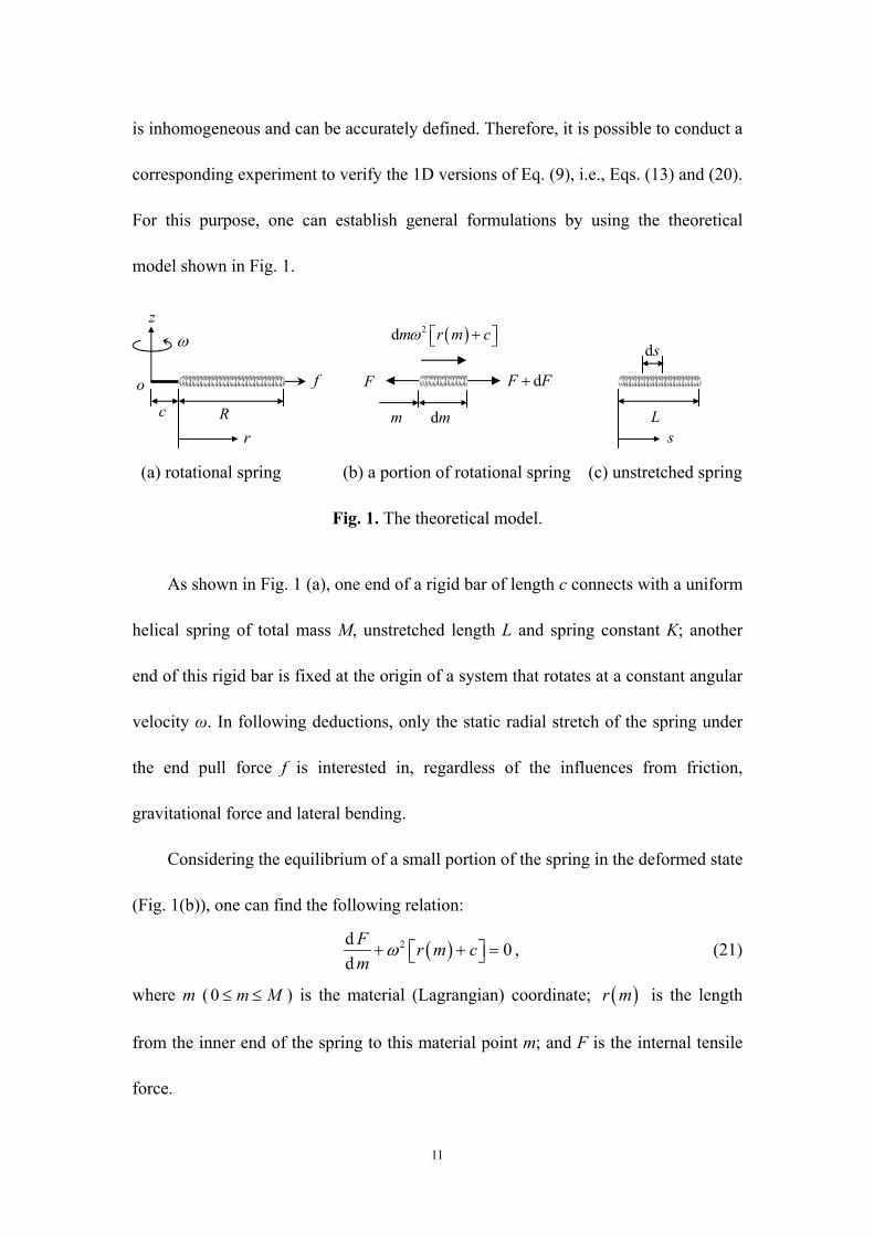
model shown in Fig. 1.

(a) rotational spring (b) a portion of rotational spring (c) unstretched spring

Fig. 1. The theoretical model.

As shown in Fig. 1 (a), one end of a rigid bar of length c connects with a uniform

helical spring of total mass M, unstretched length L and spring constant K; another

end of this rigid bar is fixed at the origin of a system that rotates at a constant angular

velocity ω. In following deductions, only the static radial stretch of the spring under

the end pull force f is interested in, regardless of the influences from friction,

gravitational force and lateral bending.

Considering the equilibrium of a small portion of the spring in the deformed state

(Fig. 1(b)), one can find the following relation:

2d0

d

Fr m c

m , (21)

where m ( 0 m M ) is the material (Lagrangian) coordinate; r m is the length

from the inner end of the spring to this material point m; and F is the internal tensile

force.

Ls

ds

m dm

F dF F

2dm r m c z

R

o f

c

r

12

Denote the unstretched length of dm portion of the spring as ds (Fig. 1(c)), which

satisfies d / d /s L m M , because the mass of the unstretched spring is uniformly

distributed. It is easy to prove that the corresponding spring constant of this uniform

portion is / dKL s . Since this portion deforms from the uniform unstretched state

free of pretension, one can use the Hooke’s Law to obtain:

dd d

d d

L rF m K r s K M L

s m

. (22)

Substituting Eq. (22) into Eq. (21), yields:

2 2

2

d0

d

rr c

m MK

. (23)

Noticing the boundary conditions of 0 0r and F M f , one can easily find

the solution of Eq. (23):

tan sin cos 1cos

f KL q qr m c q m c m

Kq q M M

, (24a)

where

Mq

K . (24b)

Eq. (24) explicitly shows that this rotational spring is inhomogeneous.

Substituting Eq. (24a) into Eq. (22), yields:

tan cos sincos

f KL q qF m cKq q m cKq m KL

q M M

. (25)

One can notice that Eq. (21) is the equation of motion established on the

deformed state, and Eq. (22) is the constitutive equation free of pretensions. Therefore,

Eq. (23) is similar to the Lamé-Navier equation established on the deformed state, so

that Eqs. (24) and (25) are the exact solutions of this finite deformation problem.

13

Assuming 2 1q , Weinstock (1964) used the similar model to explain why the

equation of the period of a spring-mass system 2 /aM K should be corrected by

using a modified end mass * / 3a aM M M , where aM is the real attached end

mass. However, regardless of this assumption, one can exactly obtain the 1D

Willis-form equations from Eqs. (24) and (25) as follows.

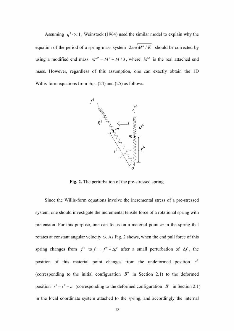
Fig. 2. The perturbation of the pre-stressed spring.

Since the Willis-form equations involve the incremental stress of a pre-stressed

system, one should investigate the incremental tensile force of a rotational spring with

pretension. For this purpose, one can focus on a material point m in the spring that

rotates at constant angular velocity ω. As Fig. 2 shows, when the end pull force of this

spring changes from 0f to 1 0f f f after a small perturbation of f , the

position of this material point changes from the undeformed position 0r

(corresponding to the initial configuration 0B in Section 2.1) to the deformed

position 1 0r r u (corresponding to the deformed configuration 1B in Section 2.1)

in the local coordinate system attached to the spring, and accordingly the internal

14

tensile force at this material point changes from 0F to 1 0F F F . The next two

sections try to check if the relation between F and u and the equation of motion

with respect to F at the undeformed position 0r are in Willis forms.

2.3. The constitutive equation in Willis form

According to Eqs. (24a) and (25), one can obtain the incremental tensile force at

material point m as:

F K u , (26a)

where

cotq

K q m KM

(26b)

denotes the effective spring constant at angular velocity ω.

Eq. (26) is the exact solution of this finite deformation problem, which is defined

at the deformed position 1r . However, 1r is unknown in the linear approximation

model, in which everything should be defined at the undeformed position 0r . For this

purpose, the tensile force of material point m at 0r can be represented as:

1 0

1 1 1 00

d

d

F rF r F r u

r , (27)

where 1 0 1 0 1, ,F r F r m f is the tensile force of an adjacent material point m

at position 0r in 1B . This means the tensile force of m is closely related to the

tensile force of m , which clearly demonstrates the non-local property of

inhomogeneous media.

Since the existing pretension 0 0F r at 0r is independent of the small

perturbation f , 1 0 1, ,F r m f equals to an incremental tensile force superimposed

15

on the pretension:

1 0 1 0 0, , tF r m f F r K u , (28)

where tK represents the tangent spring constant at 0r in 0B , and tK u is the

incremental tensile force due to the change of the configuration induced by the small

perturbation f :

0 0,

t

r r f f

F F mK u f

f m f

, (29)

where /F f f represents the direct increment due to the change of end pull

force f; and / /F m m f f represents the indirect increment due to the

change of material point from m to m at 0r .

According to Eq. (25), at the given material point m,

cos

cos

qm

F Mf q

; (30a)

and at the given configuration, i.e., for the given f,

2

tan sin coscos

F f KL q q qc q m c m K

m Kq q M M M

. (30b)

According to Eq. (24a), at the given spatial position,

2

tan cot coscos

f f KL q q Kc c q m q

m Kq q M M

; (30c)

and for the displacement u of the given material point m,

cos

sin

Kq qf u

qm

M

. (30d)

Substituting Eq. (30) into Eq. (29), yields:

16

0

0

tancos

sin costan tancos

t

f KLc q

Kq q qKK

q qf KL q m mc q mM MKq q M

. (31)

Substituting Eq. (28) into Eq. (27), yields:

0 0 0 0

1 1 0 00 0

d d

d d

t

t t

F r K u F rF F r F r K u u K u u

r r

, (32)

where the gradient of the tensile force in 0B is:

0

0 0

0

d d

d d f f

F r F m

r m r

. (33)

At the given configuration, i.e., for the given f, according to Eq. (24) one can define:

d 1

dtan cos sin

cos

mB f

r f KL q q q qc q m c m

Kq q M M M M

. (34a)

According to Eq. (24), Eq. (30b) can be further simplified as

2Fr c

m

. (34b)

Substituting Eq. (34) into Eq. (33), obtains:

0 0

2 0 00

d

d

F rB f r c

r . (35)

Eq. (32) is the linear relation defined at the undeformed position 0r . However,

one can easily prove that it is a very accurate approximation of the nonlinear solution

of Eq. (26), i.e.,

0 0

0

d

dt

F rK K

r . (36)

Denoting the cross-sectional area of the spring as A, the effective incremental

Cauchy stress as /F A , and the effective pre-stress as 0 0 /F A , Eq. (32)

can be rewritten as:

17

0

0

d

dtK u

uA r

. (37)

In addition, the displacements of the material point m and its adjacent material point

m are 1 0u m r m r m and 1 0u m r m r m , respectively.

Therefore, according to Eqs. (24a) and (34a), one can find the relation:

0

0 0 0

dlim cot

d m m

u m u mu q qe B f m u

r r m r m M M

. (38)

Substituting Eqs. (31), (34a) and (38) into Eq. (37), yields:

00

0

d

dC e u

r

, (39a)

where

00 sin

cos cos

f KL cKq qC

qA q m

M

. (39b)

This is exactly a 1D constitutive equation in Willis form, in accordance with Eq. (13).

Similar to Section 2.1, one can also obtain Eq. (39a) from the energy point of

view, if noticing the strain energy density of material point m equals to the work done

by the pre-stress 0 1r and the deformation stress 0C e :

0 0

0 1 0 2 0 0 0 20

d1 1

2 d 2

rW r e C e r u e C e

r

. (40)

2.4. The equation of motion in Willis form

According to Eq. (35) and noticing 0 0 /F A and 1 1 /F A , one can

obtain the equations of motion of material point m in 0B and 1B :

0 2

0 00

d0

dB f r c

r A

, (41)

18

1 2

1 11

d0

dB f r c

r A

. (42)

In Eq. (42), 1 0 1

1 1 0

d d d

d d d

r

r r r

, 1 0 , 1 0r r u and 1B f can be denoted

as 1 0B f B f B . If f is very small, , u and B are also very small.

Therefore, substituting these relations into Eq. (42) and noticing Eq. (41), one obtains

0 20 0

0 0 0

0 20 0

0 0

d d d1 0

d d d

d d

d d

uB f B r u c

r r r A

e B f u r c Br r A

, (43)

which is exactly the 1D version of Eq. (9b) free of the additional external body force.

And

00

f f

B BB u f

r f

, (44)

where 0/B r u represents the increment due to the change of position and

/B f f represents the increment due to the change of end pull force f.

According to Eq. (41), one can obtain:

0

0 02 0 2 20 0

2 0 00

dd

dd f f

B f r c Bu u B f r c u

A r A rr

. (45)

According to Eqs. (30d) and (34a), and referring to Eqs. (38) and (41), it is easy to

prove:

0

2 00

0

d

df f

r c Be f

r A f

. (46)

Then, adding Eq. (45) with Eq. (46) and noticing Eq. (44), yields

2 0 0 20 0

2 00

d d

ddu e B f u r c B

r Ar

. (47)

Therefore, Eq. (43) can be written as:

19

0 2 0

20 0 0

d d d2

d d de u

r r r

, (48)

which is in accordance with Eq. (20).

Similar to Section 2.1, Eq. (48) can also be obtained from the Euler-Lagrange

equation, if noticing Eq. (40), 20 0 2 0 0 2d / d d / d / 2V r u r u and

0 0d /dnlV r eu .

2.5. Discussions

From Eq. (24a), one can obtain:

2sincot 1 cos 1 cot cot

cos

qf q q KL c q q q K q q K R L

q

, (49)

where R r M is the full length of the stretched spring. This equation has the

different form as the Hooke’s law f K R L , unless 0q . In addition, based on

Eq. (49) one can obtain the incremental relation cotf q q K R . Although it has

the same form as the Hooke’s law f K R , the effective spring constant

cotq q K contains ω, a property of the rotating frame, so that it is not frame

independent (Frewer, 2009). All in all, this demonstrates that the Hooke’s law violates

the PMFI under a rotation transformation if the spring mass can not be ignored.

Eq. (24) reveals that the spring is generally inhomogeneous, so that it naturally

follows the 1D Willis-form equations of (39a) and (48). These equations will

degenerate to the Hooke’s law if the rotation velocity is zero or the spring mass is

ignored, because in these cases 0q , and hence tK K and 0 0d / d 0F r .

In practice, the end pull force f can be conveniently generated by attaching an

end mass aM at the outer end of the spring. In this way,

20

2af M c R d , (50)

where d is the distance between the outer end of the spring and the barycenter of the

attached mass. The f can be generated by either change the attached end mass M

or change the angular velocity ω. Since f is the function of the unknown R, this is a

finite deformation problem, i.e., the F in Eq. (26) is not only related to the known

0r but also related to the unknown u due to F . Usually, it is very difficult to

analytically solve a finite deformation problem. Instead, one has to piecewisely

linearize this nonlinear problem and uses only tangent predictions (e.g., calculate f

by Eq. (50) while using 0R R ) to obtain approximate solutions iteratively, which

are always suffered from the well-known drifting effect. However, for this simple case

of a rotational heavy spring, it does possible to obtain the analytical solutions. The

K in Eq. (26) can be regarded as the exact secant spring constant, which can be

decomposed into the tangent spring constant tK plus the gradient of the tensile force

0 0d / dF r according to Eq. (36). Consequently, Eq. (39a) is the 1D constitutive

equation in Willis form. Experimental results in Section 3.2 will give further

demonstrations of the importance of 0 0d / dF r , which can naturally explain the

spin-softening effect. In addition, the linear equation of motion should be established

on the undeformed state. Following this concept, one can obtain Eq. (48), the 1D

equation of motion in Willis form. It is also a much accurate linear approximation of

the equation of motion for the incremental stress on a pre-stressed medium. All in all,

these Willis-form equations are very accurate linear approximations of the nonlinear

equations for finite deformation problems.

21

Since the governing equations of a heavy spring change from the Hooke’s Law

to the Willis-form equations after a rotation transformation, it is necessary to verify

these new equations with experimental results before the implementation (Frewer,

2009). For this purpose, experiments are conducted in Section 3 to verify Eqs. (26)

and (49), because the Willis-form equations of (39a) and (48) are natural results from

these two equations.

3. Experimental verifications

3.1. The experiment setup

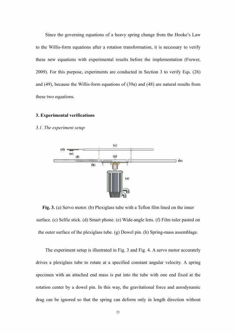
Fig. 3. (a) Servo motor. (b) Plexiglass tube with a Teflon film lined on the inner

surface. (c) Selfie stick. (d) Smart phone. (e) Wide-angle lens. (f) Film ruler pasted on

the outer surface of the plexiglass tube. (g) Dowel pin. (h) Spring-mass assemblage.

The experiment setup is illustrated in Fig. 3 and Fig. 4. A servo motor accurately

drives a plexiglass tube to rotate at a specified constant angular velocity. A spring

specimen with an attached end mass is put into the tube with one end fixed at the

rotation center by a dowel pin. In this way, the gravitational force and aerodynamic

drag can be ignored so that the spring can deform only in length direction without

22

lateral bending. In addition, since the spring-mass assemblage is in a static state

relative to the tube, the Coriolis effect is negligible. To reduce the friction force

between the spring and the inner surface of the tube, the spring diameter (12mm) is

set smaller than the inner diameter (15mm) of the tube to reduce the contact area, and

the inner surface of the tube is lined with a thin Teflon film with a very small friction

coefficient.

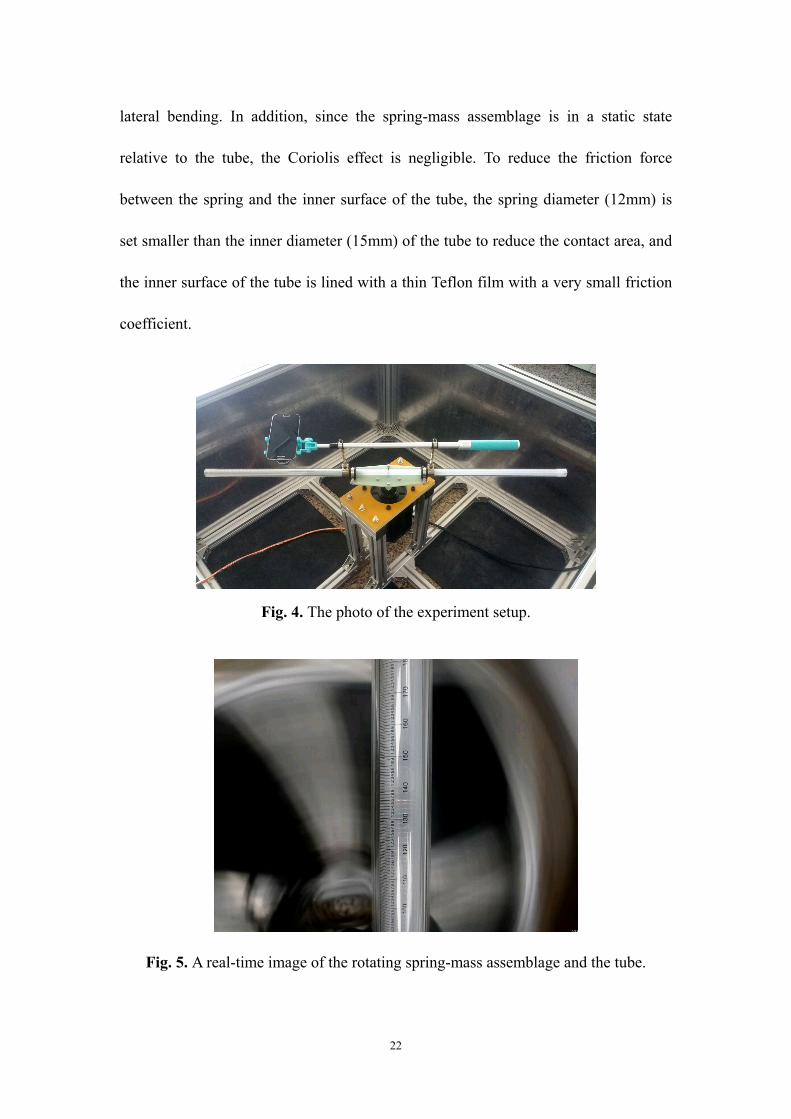
Fig. 4. The photo of the experiment setup.

Fig. 5. A real-time image of the rotating spring-mass assemblage and the tube.

23

The image of the spring-mass assemblage and the tube is recorded in real time by

a smart phone with a wide-angle lens, which is mounted on a selfie stick that rotates

along with the tube. This image is wirelessly transmitted to another smart phone a

distance away from the experiment setup through Wi-Fi. In this way, an observer can

easily measure the spring length through a film ruler pasted on the outer surface of the

tube (Fig. 5).

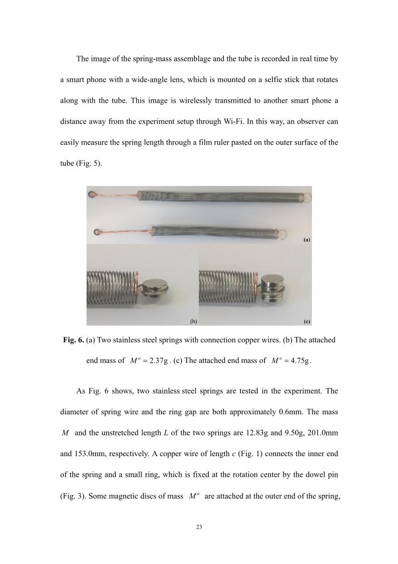
Fig. 6. (a) Two stainless steel springs with connection copper wires. (b) The attached

end mass of 2.37gaM . (c) The attached end mass of 4.75gaM .

As Fig. 6 shows, two stainless steel springs are tested in the experiment. The

diameter of spring wire and the ring gap are both approximately 0.6mm. The mass

M and the unstretched length L of the two springs are 12.83g and 9.50g, 201.0mm

and 153.0mm, respectively. A copper wire of length c (Fig. 1) connects the inner end

of the spring and a small ring, which is fixed at the rotation center by the dowel pin

(Fig. 3). Some magnetic discs of mass aM are attached at the outer end of the spring,

24

which generate the end pull force according to Eq. (50), where d is 8.0mm and 7.0mm,

and c is 64.5mm and 72.0mm for the 201mm-length spring and the 153mm-length

spring, respectively. Two attached end masses of 2.37gaM and 4.75gaM are

used to generate end pull force 0f and 1f mentioned in Section 2, respectively.

The upper half ring of the outer end of the spring is wrapped with a piece of copper

foil, which serves as a highly reflective marker to facilitate reading the scale value

(Fig. 5).

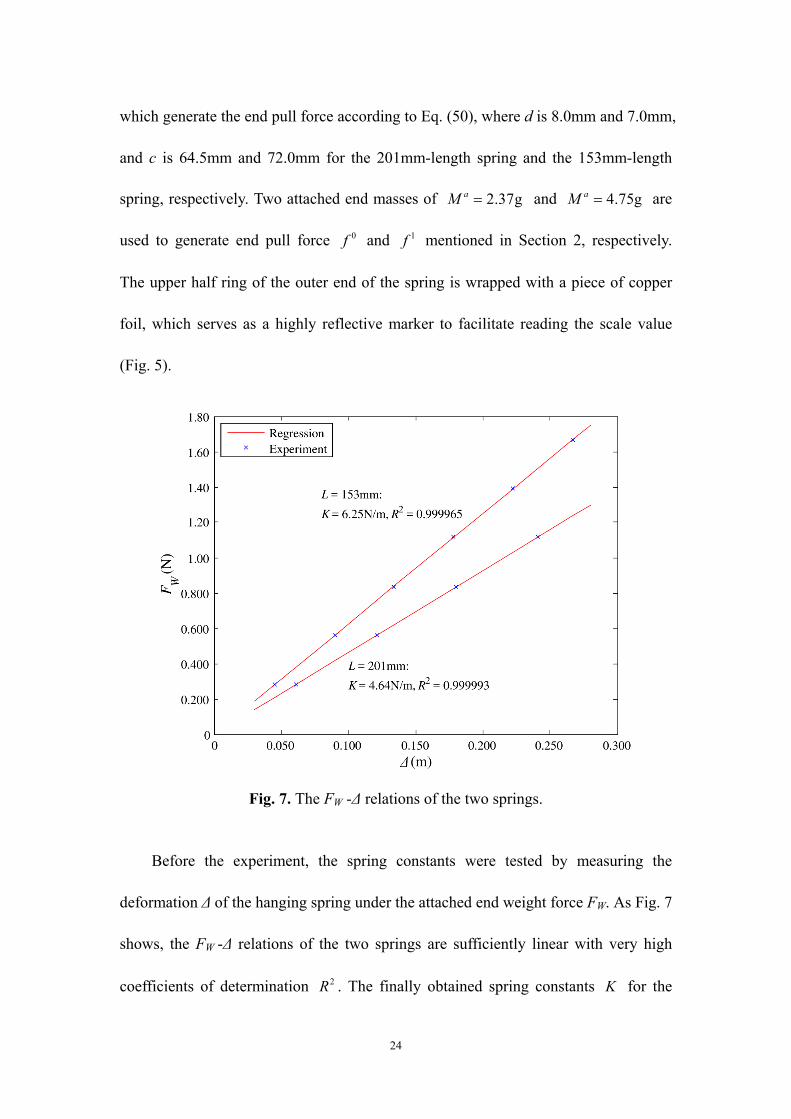
Fig. 7. The FW -Δ relations of the two springs.

Before the experiment, the spring constants were tested by measuring the

deformation Δ of the hanging spring under the attached end weight force FW. As Fig. 7

shows, the FW -Δ relations of the two springs are sufficiently linear with very high

coefficients of determination 2R . The finally obtained spring constants K for the

25

201mm-length spring and the 153mm-length spring are 4.64 N/m and 6.25 N/m,

respectively.

Each spring specimen in Fig. 6 is tested through the following steps:

Step 1: Place the spring-mass assemblage with the attached end mass of 2.37gaM

into the tube and fix it at the rotation center by the dowel pin;

Step 2: Turn on the servo motor and gradually speed it up to a relatively large angular

velocity. Keep the constant angular velocity for a moment and then gradually

slow down and turn off the servo motor. In this way, the spring is in a

naturally unstretched state. Then, one can measure c and L;

Step 3: Run the servo motor at a series of constant angular velocities and record the

corresponding spring length from the real-time image in Fig. 5. The range of

angular velocity is chosen such that the spring is sufficiently stretched within

the length limit of the tube (0.5m in this experiment setup). To ensure the

accuracy of the measurement, one should adjust the smart phone at a proper

position so that the reflective marker locates in the optical non-distorted zone,

which is about 10mm-width in the view center of the camera (Fig. 5). The

resolution of the recorded spring length is estimated to 0.1mm;

Step 4: Repeat Step 1 through Step 3 for the spring-mass assemblage with the attached

end mass of 4.75gaM .

26

3.2. The experimental results

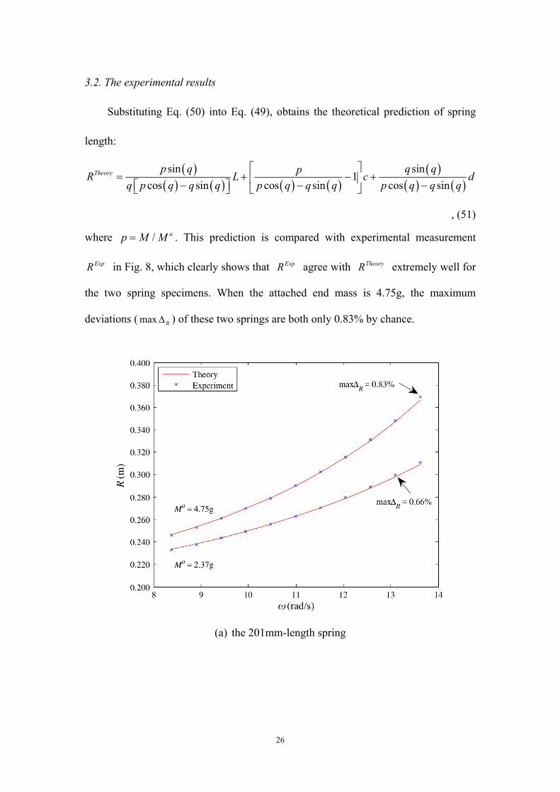
Substituting Eq. (50) into Eq. (49), obtains the theoretical prediction of spring

length:

sin sin1

cos sin cos sin cos sinTheory p q q qp

R L c dq p q q q p q q q p q q q

, (51)

where / ap M M . This prediction is compared with experimental measurement

ExpR in Fig. 8, which clearly shows that ExpR agree with TheoryR extremely well for

the two spring specimens. When the attached end mass is 4.75g, the maximum

deviations ( max R ) of these two springs are both only 0.83% by chance.

(a) the 201mm-length spring

27

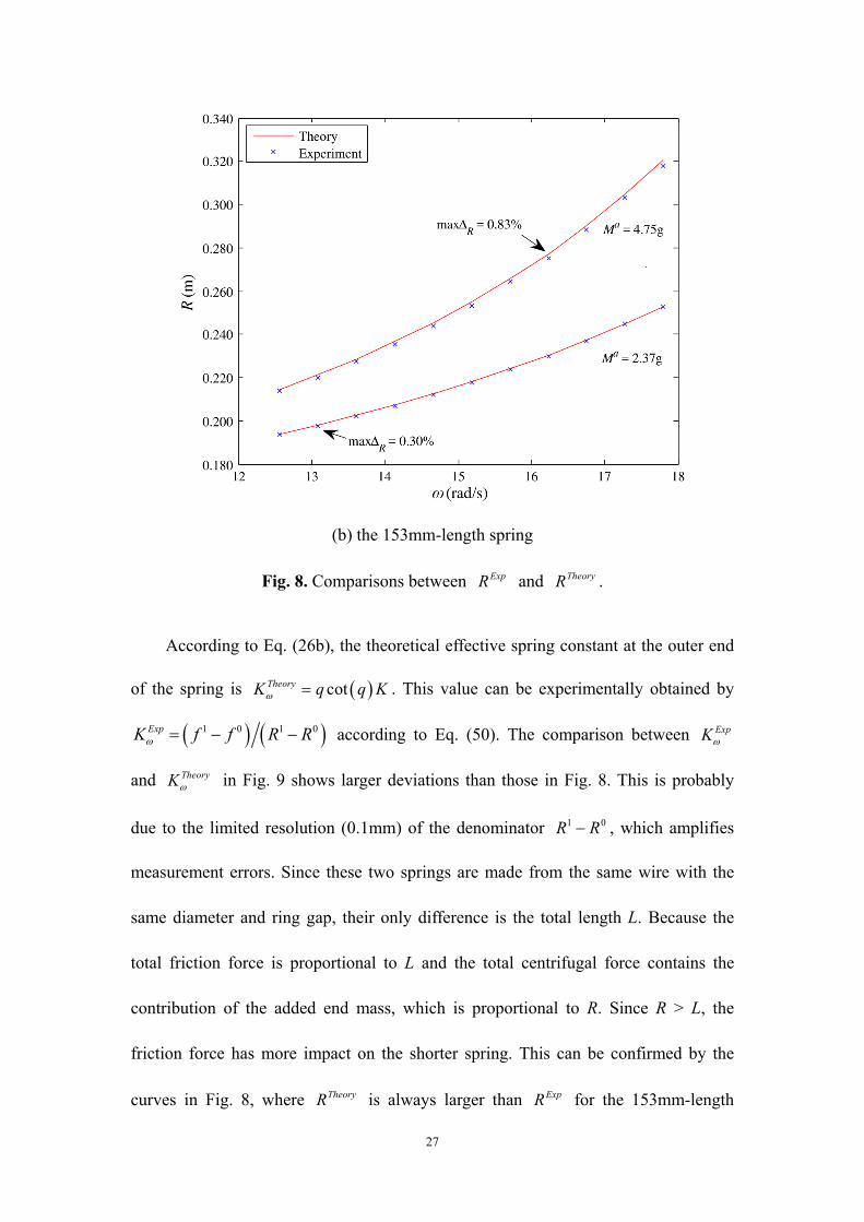
(b) the 153mm-length spring

Fig. 8. Comparisons between ExpR and TheoryR .

According to Eq. (26b), the theoretical effective spring constant at the outer end

of the spring is cotTheoryK q q K . This value can be experimentally obtained by

1 0 1 0ExpK f f R R according to Eq. (50). The comparison between ExpK

and TheoryK in Fig. 9 shows larger deviations than those in Fig. 8. This is probably

due to the limited resolution (0.1mm) of the denominator 1 0R R , which amplifies

measurement errors. Since these two springs are made from the same wire with the

same diameter and ring gap, their only difference is the total length L. Because the

total friction force is proportional to L and the total centrifugal force contains the

contribution of the added end mass, which is proportional to R. Since R > L, the

friction force has more impact on the shorter spring. This can be confirmed by the

curves in Fig. 8, where TheoryR is always larger than ExpR for the 153mm-length

28

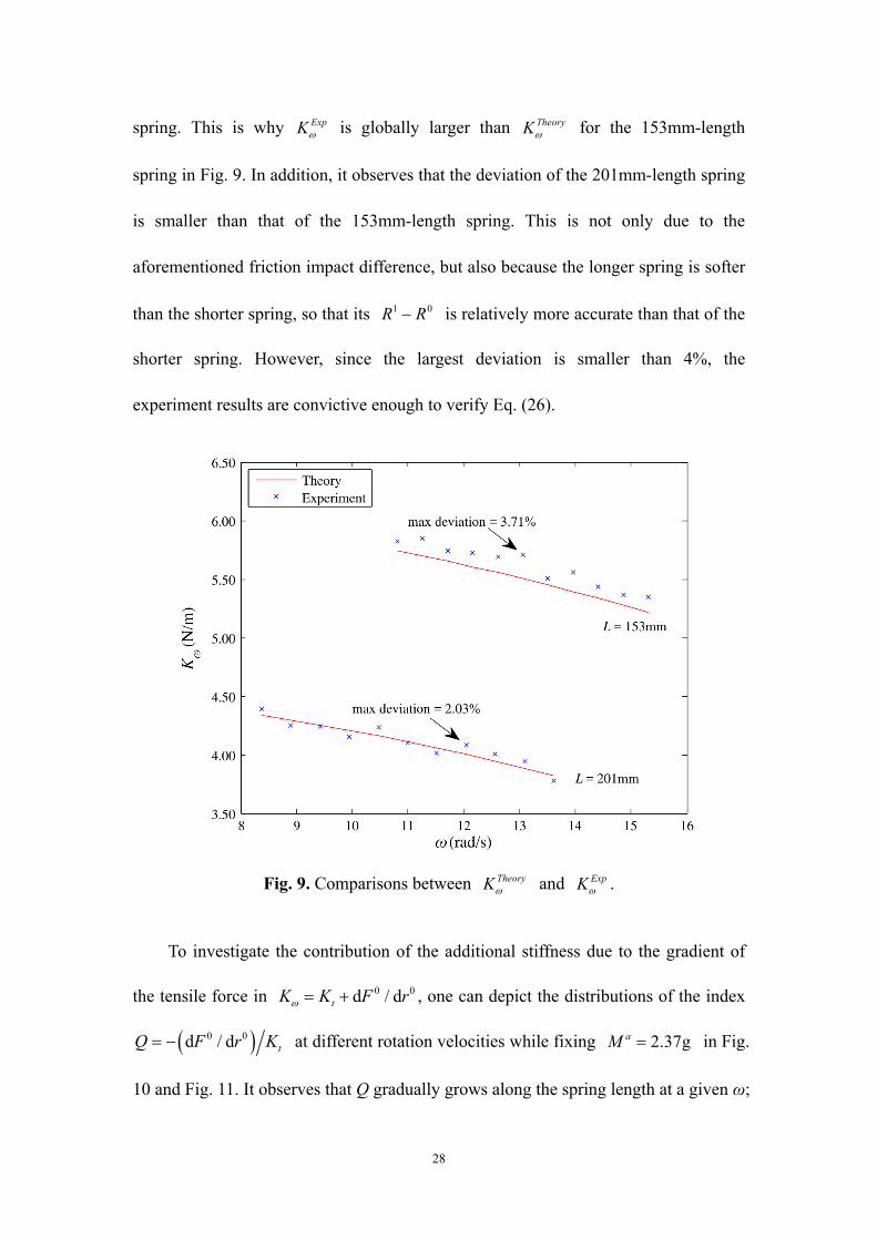
spring. This is why ExpK is globally larger than TheoryK for the 153mm-length

spring in Fig. 9. In addition, it observes that the deviation of the 201mm-length spring

is smaller than that of the 153mm-length spring. This is not only due to the

aforementioned friction impact difference, but also because the longer spring is softer

than the shorter spring, so that its 1 0R R is relatively more accurate than that of the

shorter spring. However, since the largest deviation is smaller than 4%, the

experiment results are convictive enough to verify Eq. (26).

Fig. 9. Comparisons between TheoryK and ExpK .

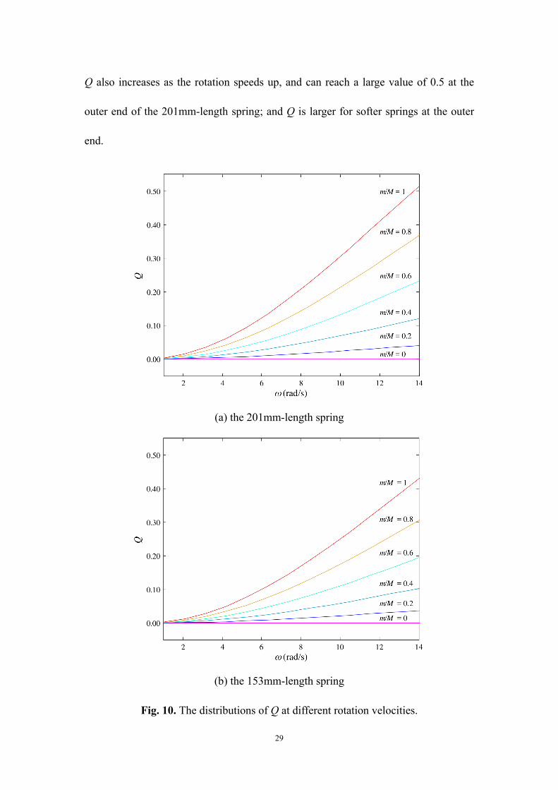
To investigate the contribution of the additional stiffness due to the gradient of

the tensile force in 0 0d / dtK K F r , one can depict the distributions of the index

0 0d / d tQ F r K at different rotation velocities while fixing 2.37gaM in Fig.

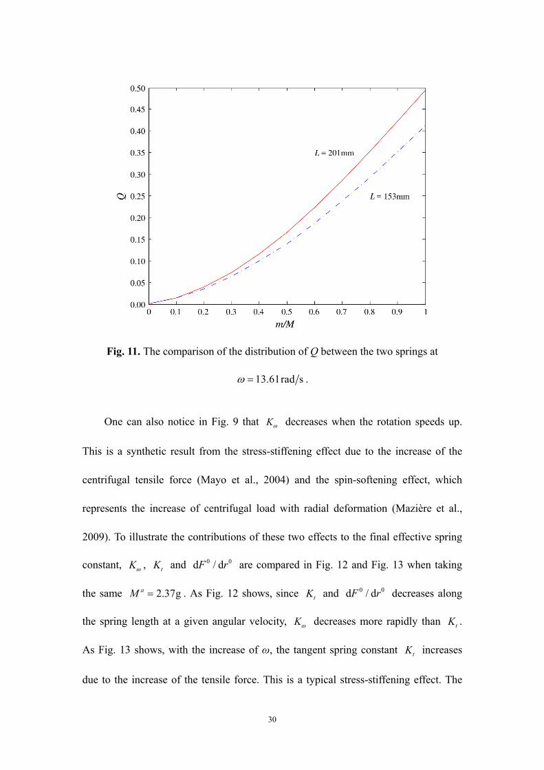
10 and Fig. 11. It observes that Q gradually grows along the spring length at a given ω;

29

Q also increases as the rotation speeds up, and can reach a large value of 0.5 at the

outer end of the 201mm-length spring; and Q is larger for softer springs at the outer

end.

(a) the 201mm-length spring

(b) the 153mm-length spring

Fig. 10. The distributions of Q at different rotation velocities.

30

Fig. 11. The comparison of the distribution of Q between the two springs at

13.61rad s .

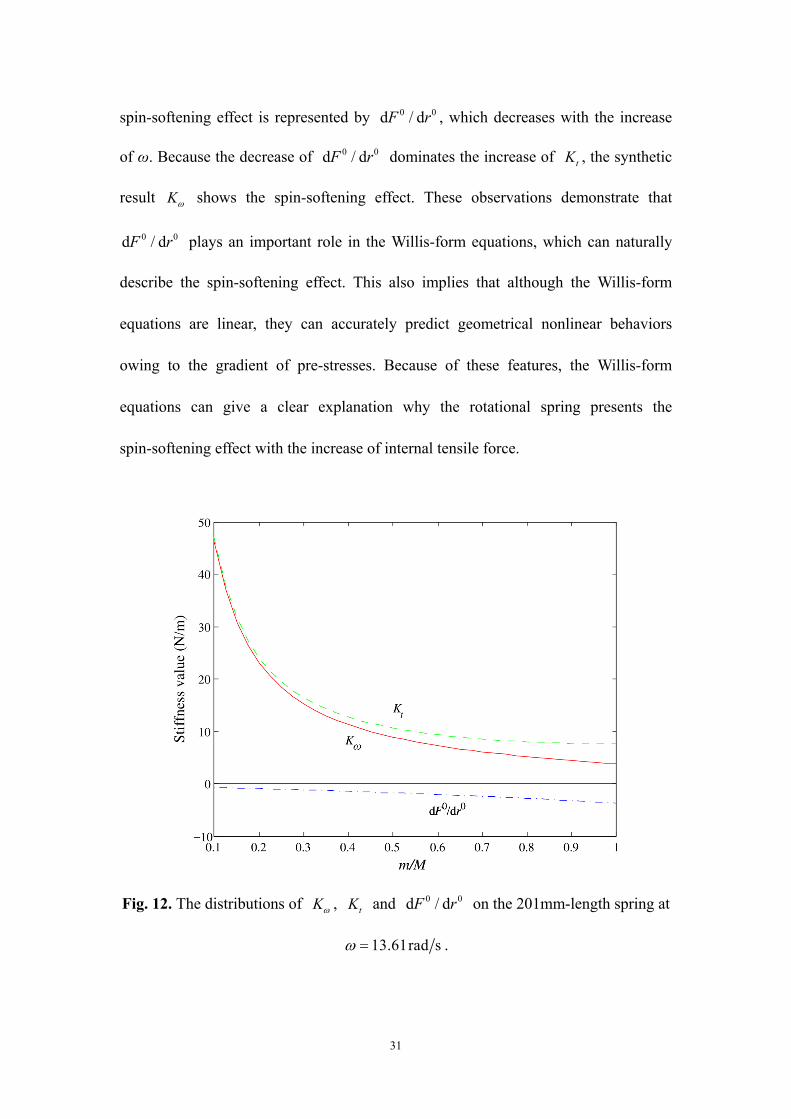
One can also notice in Fig. 9 that K decreases when the rotation speeds up.

This is a synthetic result from the stress-stiffening effect due to the increase of the

centrifugal tensile force (Mayo et al., 2004) and the spin-softening effect, which

represents the increase of centrifugal load with radial deformation (Mazière et al.,

2009). To illustrate the contributions of these two effects to the final effective spring

constant, K , tK and 0 0d / dF r are compared in Fig. 12 and Fig. 13 when taking

the same 2.37gaM . As Fig. 12 shows, since tK and 0 0d / dF r decreases along

the spring length at a given angular velocity, K decreases more rapidly than tK .

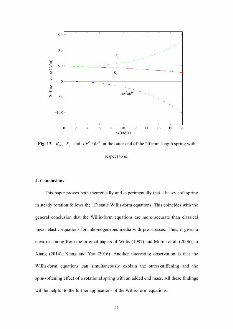
As Fig. 13 shows, with the increase of ω, the tangent spring constant tK increases

due to the increase of the tensile force. This is a typical stress-stiffening effect. The

31

spin-softening effect is represented by 0 0d / dF r , which decreases with the increase

of ω. Because the decrease of 0 0d / dF r dominates the increase of tK , the synthetic

result K shows the spin-softening effect. These observations demonstrate that

0 0d / dF r plays an important role in the Willis-form equations, which can naturally

describe the spin-softening effect. This also implies that although the Willis-form

equations are linear, they can accurately predict geometrical nonlinear behaviors

owing to the gradient of pre-stresses. Because of these features, the Willis-form

equations can give a clear explanation why the rotational spring presents the

spin-softening effect with the increase of internal tensile force.

Fig. 12. The distributions of K , tK and 0 0d / dF r on the 201mm-length spring at

13.61rad s .

32

Fig. 13. K , tK and 0 0d / dF r at the outer end of the 201mm-length spring with

respect to ω.

4. Conclusions

This paper proves both theoretically and experimentally that a heavy soft spring

in steady rotation follows the 1D static Willis-form equations. This coincides with the

general conclusion that the Willis-form equations are more accurate than classical

linear elastic equations for inhomogeneous media with pre-stresses. Thus, it gives a

clear reasoning from the original papers of Willis (1997) and Milton et al. (2006), to

Xiang (2014), Xiang and Yao (2016). Another interesting observation is that the

Willis-form equations can simultaneously explain the stress-stiffening and the

spin-softening effect of a rotational spring with an added end mass. All these findings

will be helpful to the further applications of the Willis-form equations.

33

Acknowledgment

This work was supported by the National Science Foundation of China [grant

numbers 11672144, 11272168].

References

Chen, H., Chan, C.T., 2010. Acoustic cloaking and transformation acoustics. J. Phys.

D: Appl. Phys. 43, 113001.

Frewer, M., 2009. More clarity on the concept of material frame-indifference in

classical continuum mechanics. Acta Mech. 202, 213-246.

Kienzler, R., Herrmann, G., 2000. Mechanics in material space. Springer-Verlag,

Berlin.

Leonhardt, U., 2006. Optical conformal mapping. Science 312, 1777-1780.

Milton, G.W., Briane, M., Willis, J.R., 2006. On cloaking for elasticity and physical

equations with a transformation invariant form. New J. Phys. 8, 248.

Mayo, J.M., García-Vallejo, D., Domínguez, J., 2004. Study of the Geometric

Stiffening Effect: Comparison of Different Formulations. Multibody System

Dynamics 11, 321-341.

Mazière, M., Besson, J., Forest, S., Tanguy, B., Chalons, H., Vogel, F., 2009.

Overspeed burst of elastoviscoplastic rotating disks - Part I: Analytical and numerical

stability analyses. European Journal of Mechanics - A/Solids 28, 36-44.

Nassar, H., He, Q.C., Auffray, N., 2015. Willis elastodynamic homogenization theory

revisited for periodic media. Journal of the Mechanics and Physics of Solids 77,

158-178.

34

Nassar, H., He, Q.C., Auffray, N., 2016. On asymptotic elastodynamic

homogenization approaches for periodic media. Journal of the Mechanics and Physics

of Solids 88, 274-290.

Norris, A.N., Shuvalov, A.L., Kutsenko, A.A., 2012. Analytical formulation of

three-dimensional dynamic homogenization for periodic elastic systems. Proc. R. Soc.

A. 468, 1629-1651.

Olver, P.J., 1993. Applications of Lie groups to differential equations, 2nd Ed. Springer,

New York.

Pendry, J.B., Schurig, D., Smith, D.R., 2006. Controlling electromagnetic fields.

Science 312, 1780-1782.

Torrent, D., Pennec, Y., Djafari-Rouhani, B., 2015. Resonant and non-local properties

of phononic metasolids. Physical Review B 92, 174110.

Shamonina, E., Solymar, L., 2007. Metamaterials: How the subject started.

Metamaterials 1, 12-18.

Srivastava, A., Nemat-Nasser, S., 2012. Overall dynamic properties of

three-dimensional periodic elastic composites. Proc. R. Soc. A. 468, 269-287.

Srivastava, A., 2015. Elastic metamaterials and dynamic homogenization: a review.

International Journal of Smart and Nano Materials 6, 41-60.

Truesdell, C., Noll, W., 2004. The non-linear field theories of mechanics, 3rd Ed.

Springer, Heidelberg, 44-47.

Weinstock, R., 1964. Spring-mass correction in uniform circular motion. American

Journal of Physics 32, 370-376.

35

Willis, J.R., 1981. Variational principles for dynamics problems in inhomogeneous

elastic media. Wave Motion 3, 1-11.

Willis, J.R., 1997. Dynamics of composites continuum micromechanics, in Suquet, P.

(Eds.), Continuum micromechanics: CISM Courses and Lectures No. 377.

Springer-Verlag, Berlin, pp. 265-290.

Willis, J.R., 2011. Effective constitutive relations for waves in composites and

metamaterials. Proc. R. Soc. A. 467, 1865-1879.

Xiang, Z.H., 2014. The form-invariance of wave equations without requiring a priori

relations between field variables. SCIENCE CHINA Physics, Mechanics &

Astronomy 57, 2285-2296.

Xiang, Z.H., Yao, R.W., 2016. Realizing the Willis equations with pre-stresses.

Journal of the Mechanics and Physics of Solids 87, 1-6.