An experimental study of trading volume and divergence of expectations around earnings announcement
33
An experimental study of trading volume and divergence of expectations around earnings announcement DINH Thanh Huong, IRG - University Paris XII Val-de-Marne GAJEWSKI Jean-François, IRG - University Paris XII Val-de-Marne 1 Abstract The objective is to study from an experimental point of view investors’ reaction at the announcement of the annual earnings in terms of trading volume. Annual net income is seen by shareholders as the most important figure, since it is, for individual accounts, the basis of appropriation of profit by the shareholders’ general meeting. In the experiment, it is announced at the end of 8 rounds of exchange. Every two periods, a fraction of the annual income is revealed to all the participants. Thus, they revise periodically their expectations of the annual results. The experiment shows that the divergence of expectations does not lower when the investors have more and more information about the final results. This is the main explanation for transactions in our experimental asset markets. However, too large a divergence prevents the investors from trading. As expected, price changes in absolute value influence trading volume. But this effect is smaller than the impact of heterogeneity of expectations. JEL Classification: C91 – D84 Key-words: trading volume, heterogeneity of expectations, earnings announcement and experimental asset markets. Second version: June 2005 1 IRG (Institut de Recherche en Gestion – Université Paris XII Val-de-Marne – 61 avenue du Général de Gaulle - 94010 Créteil cedex – France (Tél. : 33 1 41 78 47 52 – Fax : 33 1 41 78 47 34)). Email: [email protected] and [email protected] . The experiments have been made at CIRANO (Center for Interuniversity Research and Analysis on Organizations). We are indebted to Claude Montmarquette for his precious help and Julie Héroux for technical assistance in conducting this research. Financial support for this research was provided by IRG and CDC Institute for Economic Research (Caisse des Dépôts et Consignations). We especially thank Isabelle Laudier. Finally, we have benefited from helpful comments on a preliminary version at the ISINI conference in Lille (2003), at the Northern Finance Association meeting (2004).
Transcript of An experimental study of trading volume and divergence of expectations around earnings announcement
An experimental study of trading volume and divergence of expectations around earnings announcement DINH Thanh Huong, IRG - University Paris XII Val-de-Marne GAJEWSKI Jean-François, IRG - University Paris XII Val-de-Marne 1
Abstract
The objective is to study from an experimental point of view investors’ reaction at the announcement of the annual earnings in terms of trading volume. Annual net income is seen by shareholders as the most important figure, since it is, for individual accounts, the basis of appropriation of profit by the shareholders’ general meeting. In the experiment, it is announced at the end of 8 rounds of exchange. Every two periods, a fraction of the annual income is revealed to all the participants. Thus, they revise periodically their expectations of the annual results. The experiment shows that the divergence of expectations does not lower when the investors have more and more information about the final results. This is the main explanation for transactions in our experimental asset markets. However, too large a divergence prevents the investors from trading. As expected, price changes in absolute value influence trading volume. But this effect is smaller than the impact of heterogeneity of expectations. JEL Classification: C91 – D84 Key-words: trading volume, heterogeneity of expectations, earnings announcement and experimental asset markets.
Second version: June 2005
1 IRG (Institut de Recherche en Gestion – Université Paris XII Val-de-Marne – 61 avenue du Général de
Gaulle - 94010 Créteil cedex – France (Tél. : 33 1 41 78 47 52 – Fax : 33 1 41 78 47 34)). Email: [email protected] and [email protected]. The experiments have been made at CIRANO (Center for Interuniversity Research and Analysis on Organizations). We are indebted to Claude Montmarquette for his precious help and Julie Héroux for technical assistance in conducting this research. Financial support for this research was provided by IRG and CDC Institute for Economic Research (Caisse des Dépôts et Consignations). We especially thank Isabelle Laudier. Finally, we have benefited from helpful comments on a preliminary version at the ISINI conference in Lille (2003), at the Northern Finance Association meeting (2004).
Trading volume and divergence of expectations around earnings announcements 2
1. Introduction
Under efficient market hypothesis, stock prices instantaneously incorporate the whole
set of available information. Thus, they reflect the fundamental stock value. Beyond
efficient market theory, the theorem of no trade predicts that if prices immediately
adjust to a change of fundamental value after any information revelation, no trade
should occur. This theorem refers to the risk-neutral rational expectations model without
asymmetric information.
Under these conditions, there are trades only when the investors anticipate a change in
asset value or have no common knowledge or have biased expectations. According to
the first condition, theoretical and empirical studies show that prices cause trades. From
a theoretical point of view, by Kim and Verrecchia (1991) demonstrate that trading
volume around earnings announcements is proportional to absolute price changes.
According to Karpoff’s survey (1987), an increase of absolute prices should be
associated with a rise in trades.
According to the second condition, the lack of common knowledge between traders, due
to asymmetric information or beliefs’ heterogeneity, could explain trades around
earnings announcements (Kandel and Pearson, 1995; Bamber, Barron and Stober,
1999). The divergence of interpretations concerns either the difference in sets of
information owned by the investors at the time of publication or the heterogeneity of
beliefs on the basis of the same set of information. The first situation appears when
there is asymmetric information between traders. In this case, trading volume is an
increasing function of absolute price changes and the precision of investors’ private
signals. In a heterogeneous structure of information, it may be possible to infer
information from trades not revealed by prices. A large change of trading volume could
signal the presence of informed traders on financial markets. Other papers (Kandel and
Pearson, 1995) make the assumption of a homogeneous structure of information. All the
investors receive the same information (for example the annual results). Thus, trading
volume is explained by the dispersion in initial beliefs and the idiosyncratic
interpretations of information. Ziebart’s (1990) paper characterizes this second
component as the mean revision of expectations due to the announcement.
Trading volume and divergence of expectations around earnings announcements 3
Bamber and al. (1997) characterize opinion dispersion, called investors’ disagreement,
by the three following factors: initial beliefs’ dispersion (the variance of expectations
preceding the announcement), the change of this dispersion (the difference between the
dispersion after and before the announcement) and the jumbling of beliefs (the change
of one investor’s beliefs relatively to others’).
However, empirical studies are unable to directly measure the heterogeneity of
investors’ beliefs. They are estimated by the dispersion of financial analysts’ forecasts
around the announcement. This proxy can be put into question as financial analysts
represent a small fraction of the whole set of economic agents (Atiase and Bamber,
1994). Moreover, they have positions different from the other agents. They are often
more informed and more qualified than the individual investors. Finally, their behaviour
strictly depends on their interests and utility functions. This induces specific biases, like
overoptimistic bias.
In this context, the experimental method may be of particular interest for this kind of
research. The effects can be observed directly in a controlled environment and the
variables influencing trading volume can be isolated from other effects, which cannot be
done in traditional empirical works.
The objective is thus to study the path of trading volume around earnings announcement
by using the experimental method. There are three main contributions. First, traders’
heterogeneous expectations are considered instead of being approached by financial
analysts’ forecasts. Second, the experimental methodology isolates the heterogeneity of
expectations from asymmetric information as all the investors own the same set of
information. The net income is published after the revelation of 4 quarterly results every
two periods. The continuous flow of public information makes it possible to study the
path of trades around earnings announcement. Third, this structure of homogeneous
information allows us to analyze further the links between trading volume, stock price
variation and the heterogeneity of expectations. This relation is checked in a deeper way
with different degrees of divergence between analysts’ forecasts. Two structures of
information are built with different standard deviations. The second structure of higher
standard deviation should logically lead to a higher divergence of investors’
expectations. Instead of an increasing linear function, we observe a concave relation
between trading volume and the divergence of expectations.
Trading volume and divergence of expectations around earnings announcements 4
In spite of a common structure of information, the experiment shows that there are
trades between the participants. These trades are explained by stock price changes and
the heterogeneity of expectations. The second element is the main explaining factor of
trades, when the divergence is not too high. Above a given threshold, the divergence
does not lead to any trade. Conversely, the average change of investors’ anticipations
does not influence trades. The present study also puts forward an effect of prices on
trades, which strengthens some prior works concluding that absolute price changes
should entail portfolio reallocation. It also appears that divergent expectations may
emerge even in a world of homogeneous information, a result similar to Gillette et al.
(1999). According to these results, some investors do not seem to believe in a rational
reaction of other agents and submit orders. As a consequence, market uncertainty
depends not only on the process of how to determine the fundamental stock value but
also on agents’ motivations. They warrant liquidity of our experimental asset markets.
For example, an optimistic trader willing to buy may not find any counterpart if no other
trader wants to sell in the same period.
2. Research hypotheses
Obviously, interim figures are actually perceived as an imprecise indicator of the annual
results. The picture becomes more and more detailed as the year’s end approaches.
According to this logic, as the number of periods increase and the publication of the
final results approaches, the earnings expectations should become more and more
homogeneous and converge towards the value of the earnings.
Hypothesis 1: Participants’ estimations of the final results converge towards the
annual results as the number of periods increase. This convergence is all the faster as
interim results are announced.
The heterogeneity of investors’ earnings expectations positively affects trading volume,
when it is not too strong. Beyond a given threshold, the probability of two opposite
orders to be matched lowers. When the expectations differ too much from one investor
to another, the placing orders should be widely different. At the highest, the investors
would take into account other agents’ behaviour, which makes the orders converge in
the same sense and lowers the amount of trades. This suggests that there exists a
Trading volume and divergence of expectations around earnings announcements 5
threshold of divergence under which the heterogeneity positively affects trading
volume. Above it, the impact of divergence on trading volume becomes negative.
Hypothesis 2: the relation between trading volume and divergence of investors’
expectations is concave.
In the present study, several degrees of dispersion are considered as two different
structures of information. The first is built in order to entail less uncertainty than the
other. Participants’ earnings expectations should be logically less heterogeneous in the
first structure than in the second. An increasing and linear relationship between
dispersion and trading volume should be observed in the first structure of information.
Conversely, this type of relationship should be not valid in the case of the second
structure.
Hypothesis 2.1: in the case of the first structure of information (where expectations are
not too divergent), trading volume is an increasing function of the dispersion of
investors’ earnings expectations.
Hypothesis 2.2: In the case of the second structure of information (where expectations
are very divergent), the linear increasing relationship between trading volume and
dispersion is no longer valid.
The annual results contain several components, each of which being announced every
two periods. The investors get more and more information as the experiment continues
and consequently investors’ expectations should become more and more homogeneous.
All things being equal, if hypothesis 2 is checked, as the number of periods increase, the
convergence of expectations lowers investors’ incentive to trade.
Corollary: Trading volume lowers as the experiment approaches to the end.
Copeland’s model (1976), extended by Epps and Epps (1976) and Jennings, Starks and
Fellingham (1981) proves theoretically that volume is positively related to the
Trading volume and divergence of expectations around earnings announcements 6
magnitude of the price change. Under the assumption of sequential arrival of
information, the information leads to shifts in investors’ demands, which causes trading.
This is largely confirmed by empirical studies (Karpoff, 1987 for a survey).
Hypothesis 3: The magnitude of stock price variation has a positive effect on trading
volume.
In addition, stock price deviations from the efficient price can also affect trading volume
as they determine trading gains that the investors may have at the end of the experience.
As a consequence, the magnitude of price errors should lead to more incentive to trade.
Hypothesis 4: The size of previous price errors positively influences positively trading
volume
In the hypothesis above, previous price errors are used instead of contemporaneous
ones, because contemporaneous errors are only calculated at the end of the period.
3. Methodology
This section focuses on our experimental methodology. We first describe the
experimental markets in which the above research hypotheses will be examined. We
then turn our attention to the determination of test parameters.
3.1. The description of experimental markets
Participants and incentive
Overall, the number of participants amounts to 91, divided into 11 markets. Each market
counts 7 to 10 unqualified students2. Using large markets is easier to characterize the
divergence of individual reactions. The participants have no special knowledge in
2 The present experiment only demands the participants to have reasonable scientific knowledge. No
specific knowledge is required, since several experimental studies have shown that a high level of skills is not necessary to make the experiments successful.
Trading volume and divergence of expectations around earnings announcements 7
finance. They are invited to attend an initial formation and receive detailed written
instructions3.
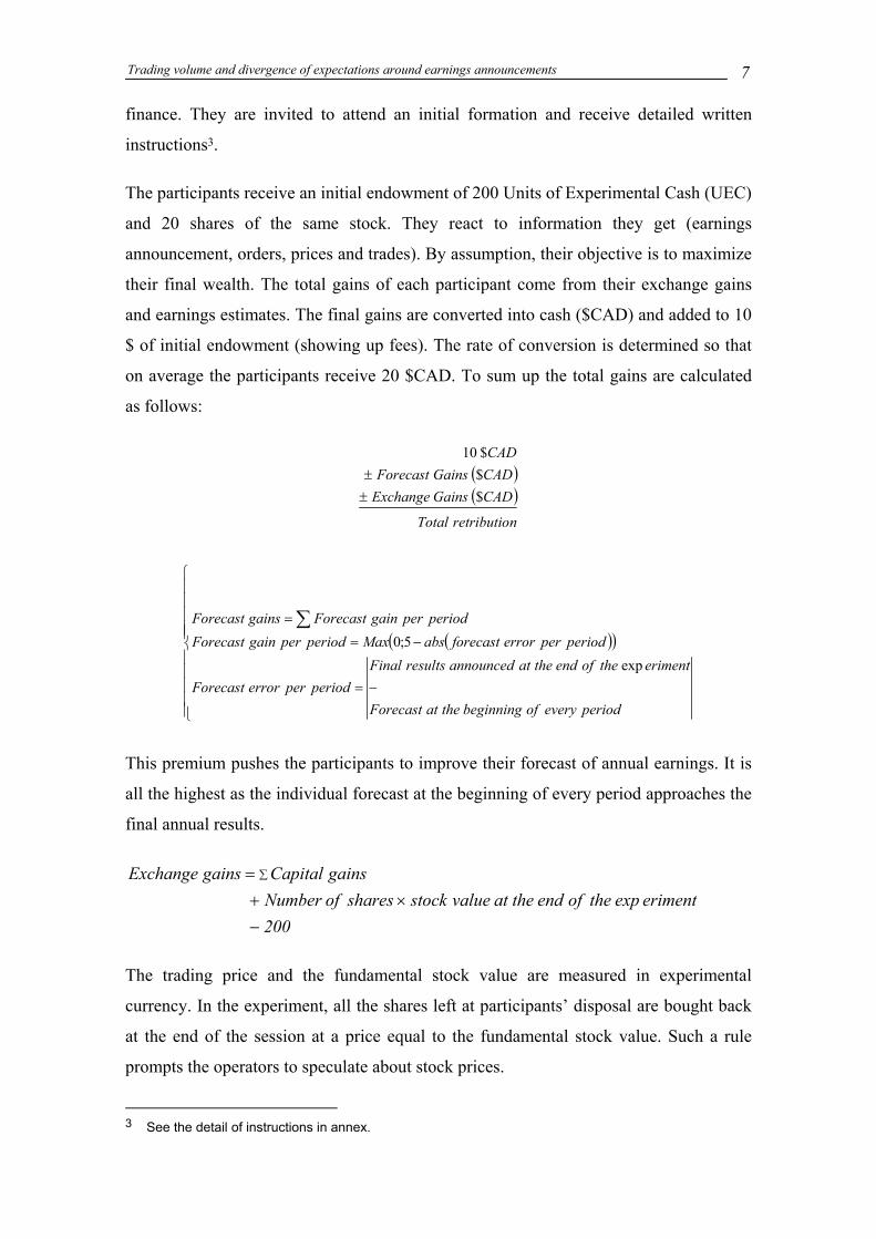
The participants receive an initial endowment of 200 Units of Experimental Cash (UEC)
and 20 shares of the same stock. They react to information they get (earnings
announcement, orders, prices and trades). By assumption, their objective is to maximize
their final wealth. The total gains of each participant come from their exchange gains
and earnings estimates. The final gains are converted into cash ($CAD) and added to 10
$ of initial endowment (showing up fees). The rate of conversion is determined so that
on average the participants receive 20 $CAD. To sum up the total gains are calculated
as follows:
( )( )
nretributioTotal
CADGainsExchangeCADGainsForecastCAD
$$$10
±±
( )( )
−=
−=
= ∑
periodeveryofbeginningtheatForecast
erimenttheofendtheatannouncedresultsFinalperiodpererrorForecast
periodpererrorforecastabsMaxperiodpergainForecastperiodpergainForecastgainsForecast
exp5;0
This premium pushes the participants to improve their forecast of annual earnings. It is
all the highest as the individual forecast at the beginning of every period approaches the
final annual results.
200erimentexptheofendtheatvaluestocksharesofNumber
gainsCapitalgainsExchange
−×+
= ∑
The trading price and the fundamental stock value are measured in experimental
currency. In the experiment, all the shares left at participants’ disposal are bought back
at the end of the session at a price equal to the fundamental stock value. Such a rule
prompts the operators to speculate about stock prices.
3 See the detail of instructions in annex.
Trading volume and divergence of expectations around earnings announcements 8
The structure of information
Conversely to the majority of previous studies, the experience here is built on a
structure of information common to all the investors4 made of a flow of information
leading to the final results. This modeling fits reality as there always exists other
sources of information before the final earnings announcement. They can be preliminary
announcements of results or estimates of the results, or interim publications.
Therefore, the results are announced after revealing 4 components. Every two periods,
one component is randomly chosen. Consequently, the investors have more and more
information as the experiment continues. As the uncertainty of the results lowers, the
investors’ earnings estimates should be more and more precise and homogeneous. If the
linear relation is valid, trading volume should decrease as the experiment approaches
the end.
Two series of information of four components are proposed. They have the same mean
but a different standard-deviation in order to generate different degrees of estimates’
dispersion. This may help to show the predicted concave relation between trading
volume and heterogeneity of expectations which may emerge from great dispersion in
expectations.
Every series of four components is inspired by Gillette and al. (1999) in terms of
determination of the value of the elements. Some differences are related to the definition
of uncertainty and the flow of information. Firstly, in Gillette’s studies, the uncertainty
about the fundamental value is only explained by the random determination of its
components. In the present paper, the uncertainty does not only lie in the determination
of the annual results but also in the relation which links the results to the fundamental
stock value. For needs of simplification, we suppose that the intrinsic value is equal to
the dividend5. The latter is equal to the last results if they are positive and zero
otherwise.
The second difference concerns the number of components and the set of values of each
component. In Gillette and al. (1999), the final value is the sum of five positive
elements whereas the final value here is the sum of four elements. This structure of
4 There is no asymmetric information between the investors during the experiment. 5 This hypothesis does not imply that the investors have the same estimation of the firm cost of capital or
the dividend growth rate.
Trading volume and divergence of expectations around earnings announcements 9
information approaches the real situation in which the quarterly results are announced
before the annual earnings. Moreover, the series may contain negative values.
Introducing negative values is of double interest. First, this means that firms may realize
losses as well as profits. Second, it may help us to measure risk preferences.
Both series of information are described as follows. For the first series, the final results
are made of 4 elements whose value is 0, 2, 4 or 6 with probabilities 1/4, 1/4, 1/4 and
1/4. These four elements are chosen at random and announced at the end of periods 2, 4,
6 and 8. Being the sum of these four elements, the final results belong to the interval [0;
24]. The dividend is distributed at the end of the experiment. For needs of
simplification, the rate of distribution is always equal to 100%. It is stable and
preannounced at the beginning of the experiment. The dividend is thus equal to the
fundamental value. At the beginning of every exchange round, the students are asked to
estimate the value of the results. The structure of information allows a regular estimate
of the results between periods 1 and 2, 3 and 4, 5 and 6, 7 and 8. These intervals are
called estimation periods. At the end of each estimation period, one element of the
series of information is randomly chosen. The mean value of each component is equal
to:
34164
144124
10 =×+×+×+×
Before the first period, the expected mean value of the results is 12 and the expected
fundamental value is thus 12. After drawing one component of the results, the objective
anticipated results become the sum of this value and the estimates of the remaining
elements. The drawing lots are executed by the computer.
For the second series of information, the determination of the annual results is similar to
the first one. However, the fundamental value is determined in a different way because
of one negative value into the set of possible values. As a matter of fact, the 4 elements
of the series may take the values –4, 0, 6, 10 with probabilities ¼, ¼, ¼ and ¼. The
anticipated mean value is thus:
341104
164104
14 =×+×+×+×−
Trading volume and divergence of expectations around earnings announcements 10
The annual results may vary from -16 to 40 with the mean value of 12. The rate of
dividend distribution is 100% if the results are positive and zero otherwise. In this case,
the fundamental value is equal to the dividend if it is positive and 0 otherwise.
The trading mechanism
Here, we use the structure of double-auction markets. This mechanism used in most
stock markets seems to be the most efficient in terms of information (Theissen (2000))
as well as in terms of allocation (Gode and Sunder (1993)). The anomalies detected in
this type of experimental market strictly correspond to the real ones because they do not
heavily depend on market microstructure. They are mainly due to the informational
attributes and the participants’ characteristics like motivations, preferences, rationality
and cognitive ability.
The experiment is completely computed. First of all, the stocks and the cash at students’
disposal are virtually registered into an account. At each round, participants submit buy
or sell limit orders. The orders (characterized by the quantity, the price and the time of
entry) continuously appear on all computer screens. They are registered in a central
computer that allows one to determine the execution price immediately. There is trade
between two investors as soon as there are opposite compatible orders. For a buy (sell)
order to be executed, any investor may submit a sell (buy) order with a price limit
inferior to p (superior to p). When two orders are given the same limit, the priority
depends on time. If not, all the orders which are similar in terms of price, quantity and
time are proportionally executed. Short-selling is prohibited. During a period, the orders
not executed may be modified or eliminated. They are not retained for the following
rounds.
The path of the experiment
11 markets of 7 to 10 students are considered. Every market contains 8 rounds of 6
minutes long, 5 of which are for trades. The results become public at the eighth round
after the announcement of 4 components. At the beginning of the first round, the
participants are invited to estimate the annual results. This estimation stage is over when
everyone has made his or her estimate. Thereafter, the participants submit orders and
Trading volume and divergence of expectations around earnings announcements 11
trade. At the end of the second round, one component of the results is randomly chosen
and made public. The objective expected results is calculated as follows:
43×+elementFirst
The objective anticipated fundamental value is therefore equal to the annual results if
they are positive and zero otherwise.
The other rounds go the same direction. When one component is made public, the
objective expected annual results are equal to the sum of the realized components plus
the objective estimates of the remaining components. The fundamental value is always
determined in the same way: it is equal to the results if they are positive and zero
otherwise. The market is completely transparent. Orders and trades are continuously
shown on the screens.
At the end of the eighth round, the last component is chosen randomly and the final
earnings are announced. This allows the fundamental stock value to be calculated and
thus the errors of investors’ expectations.
3.2. The determination of test parameters
Abnormal trading volume
Within this kind of studies, the abnormal trading volume is traditionally measured by
the difference between the amount of trades during the period under consideration and
the one estimated over the normal period on the basis of a standard model such as the
market model. In our study, the normal period is set up in a quite normal way (it is
completely possible within experimental study framework) in the sense that there are
neither released information nor liquidity needs. Under these circumstances, the market
would be characterized by the absence of trading activities, or in other words, the
abnormal trading volume is equal to zero.
Therefore, the asset exchanges occurring in the period marked by an announcement date
can be considered as the abnormal trading volume, which is thus defined as follows:
stockstotalstockstradedofNumberAV = (1)
Trading volume and divergence of expectations around earnings announcements 12
In addition to this measure which seems to be the pure indicator of trading volume, we
also consider a second proxy. In this case, the trading volume is equal to the ratio of the
total value traded to the market’s anticipated value. Here, the value of each transaction
is equal to the quantity of assets traded time the corresponding price. Concerning the
market anticipated value, it is simply expressed by the total number of stocks in the
market time the anticipated value of associated stocks. The final measure of trading
volume is derived from the second measure by modifying the denominator element.
That is, we use the final value instead of the objectively estimated market value. It
equalizes the fundamental value of stock multiplied by the total number of stocks. Being
different from the intrinsic value which is only calculated one time at the end of the
experience, rational anticipations vary all the periods. Though all three measures
mentioned above are usable, all the principal analysis and interpretations of this study is
based on the first measure whose results would be the most relevant. In reality, the stock
price can be erroneous. Its presence in the empirical tests may bias our results. It is
worth noting that the sole object of the use of two other measures is to compare our
results to those of previous studies.
Measure of the heterogeneity of expectations
The divergence of expectations is the standard deviation of individual expectations. By
contrast, the homogeneity of expectations refers to the mean revision of expectations.
Three measures are proposed in our study. The first one amounts to the percentage
variation in expectations of a period over another specified period. The next two
measures appear like the first one, except the fact that the variation in expectations is
differently normalized. We respectively use the objective anticipated value of annual
earnings and the final annual income instead of the previous anticipations. The errors of
expectations refer to the deviation of expectations from the final income normalized
either by the previous expectations, the anticipated value of earnings or by the annual
earnings.
Measure of stock price variation and price errors
As the mean revision of expectations, the average variation of stock prices is determined
in three ways. It refers to the difference between the current average price and the
Trading volume and divergence of expectations around earnings announcements 13
previous one divided respectively by the previous average price, the objective
expectations of stock intrinsic value or the final fundamental value of stock. The price
error is also calculated on the basis of the fundamental value. It is represented by three
ratios whose numerators are the difference between stock price and intrinsic value. As
regard to the denominators, they are different each other and correspond respectively to
the average price of the previous period, the objective prevision of true stock value or
the later.
4. Results and interpretations
4.1. Statistic descriptive of earnings estimates and trading volume
4.1.1. The path of the earnings estimates
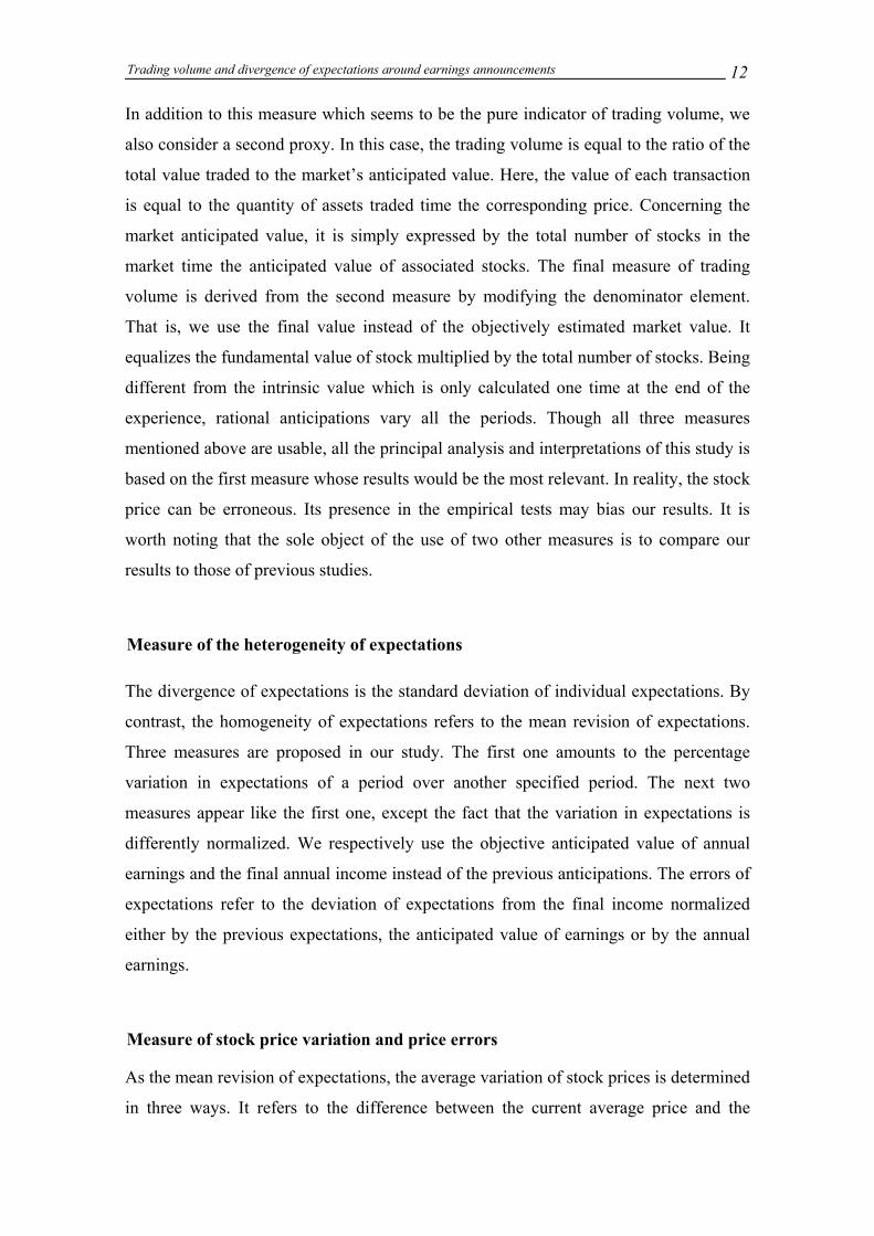
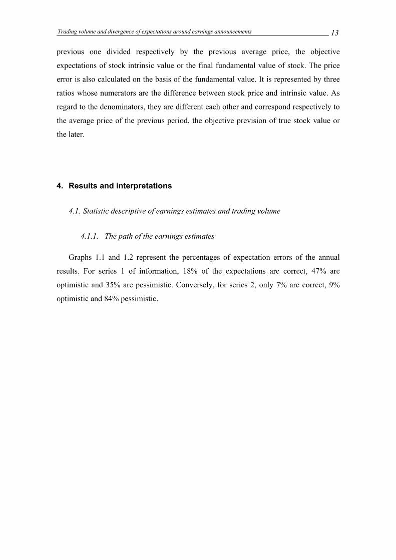
Graphs 1.1 and 1.2 represent the percentages of expectation errors of the annual
results. For series 1 of information, 18% of the expectations are correct, 47% are
optimistic and 35% are pessimistic. Conversely, for series 2, only 7% are correct, 9%
optimistic and 84% pessimistic.
Trading volume and divergence of expectations around earnings announcements 14
G r a p h 1 . 1 : d i s t r i b u t i o n o f e s t i m a t e e r r o r s ( S e r i e s 1 )
0 , 0 0
0 , 0 4
0 , 0 8
0 , 1 2
0 , 1 6
0 , 2 0
-14
-10 -8 -6 -4 -2 0 2 4 6 8 10 14
E x p e c t a t i o n e r r o r
% o
f err
ors
G r a p h 1 . 2 : d i s t r i b u t i o n o f e s t i m a t e e r r o r s ( s e r i e s 2 )
0 , 0 0
0 , 0 4
0 , 0 8
0 , 1 2
0 , 1 6
0 , 2 0
-52
-32
-28
-24
-22
-19
-17
-14
-10 -6 -4 -2 4 6 10
E x p e c t a t i o n e r r o r
% o
f err
ors
Note: these graphs are made of 728 anticipations from the 11 markets. For series 1 (series 2 respectively), 592 (136 respectively) expectations are taken into account. The unexpected errors, calculated by the difference between each estimate and the annual earnings, are represented in X-plots and the percentage of expectation errors are represented in Y-plots.
Trading volume and divergence of expectations around earnings announcements 15
Graphs 1.1 and 1.2 show that, all rounds being equal, the unexpected errors are
numerous and much dispersed. This high standard deviation of unexpected errors puts
forward that the investors do not have homogeneous anticipations, even if the
experiment runs in a structure of common information, i.e., without asymmetric
information.
The divergence of estimates can be explained only by implicit factors different from one
investor to another. Besides the diverse levels of skills and experience that directly
influence the interpretation of information, the risk preferences and cognitive
psychology can be the explanatory factors of this divergence. The dissimilar risk
preferences can play a major role in the experiment because of the uncertainty during
the experiment. This uncertainty participates to the construction of the agents’ utility
function and makes the preferences different from one agent to another. These
preferences are a major determinant of the expectations as the individuals have a great
tendency to merge their hopes with the real situation.
The effect of investors’ risk preferences on their earnings expectations would be better
defined by comparing expectations obtained from series 1 and those obtained from
series 2. Considering series 2 with a negative component of the results, the expectations
are more divergent and pessimistic than those of series 1. In average, the investors are
not mistaken in the case of series 1, because the mean expectation error is -0.03,
significantly different from zero. In the case of series 2, they are rather pessimistic with
a mean expectation error of -11.15. Series 1 exhibits a standard-deviation of 4.7,
whereas series 2 shows a standard-deviation of 10.78. As a matter of fact, the negative
component introduces further uncertainty regarding the final results. In that case, risk
preferences influence more investors’ behavior. In addition to the factor of risk
preference, the psychological and cognitive variables also explain the heterogeneity of
expectations. In fact, the overconfident investors may think that they have skills
superior to others and that others’ expectations are not correct. This leads them to form
expectations different from the market. As a result, the divergence of expectations
increases. The lack of self-confidence can also entail estimate deviations from the
fundamental value. Actually, these no self-confident investors exhibit a tendency to
infer information from others’ expectations, which leads to mistaken expectations.
Trading volume and divergence of expectations around earnings announcements 16
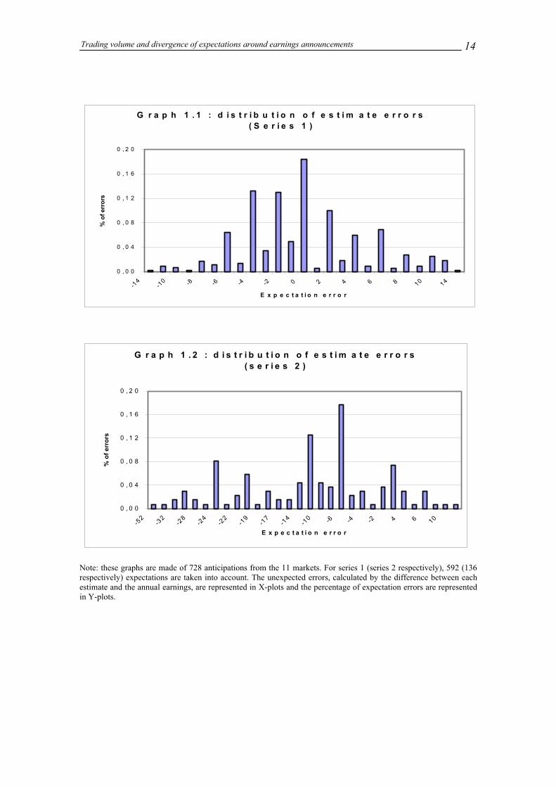
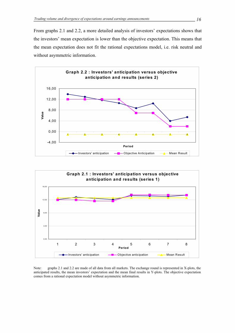
From graphs 2.1 and 2.2, a more detailed analysis of investors’ expectations shows that
the investors’ mean expectation is lower than the objective expectation. This means that
the mean expectation does not fit the rational expectations model, i.e. risk neutral and
without asymmetric information.
Graph 2.2 : Investors' anticipation versus objective anticipation and results (series 2)
-4,00
0,00
4,00
8,00
12,00
16,00
1 2 3 4 5 6 7 8
Period
Valu
e
Investors' anticipation Objective Anticipation Mean Result
Graph 2.1 : Investors' anticipation versus objective anticipation and results (series 1)
0,00
4,00
8,00
12,00
16,00
1 2 3 4 5 6 7 8Period
Valu
e
Investors' antic ipation Objective anticipation Mean Result
Note: graphs 2.1 and 2.2 are made of all data from all markets. The exchange round is represented in X-plots, the anticipated results, the mean investors’ expectation and the mean final results in Y-plots. The objective expectation comes from a rational expectation model without asymmetric information.
Trading volume and divergence of expectations around earnings announcements 17
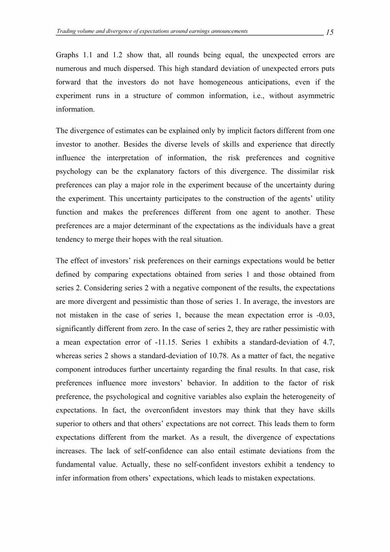
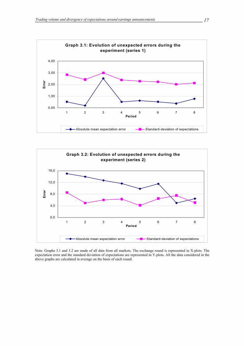
Note: Graphs 3.1 and 3.2 are made of all data from all markets. The exchange round is represented in X-plots. The expectation error and the standard deviation of expectations are represented in Y-plots. All the data considered in the above graphs are calculated in average on the basis of each round.
Graph 3.1: Evolution of unexpected errors during the experiment (series 1)
0,00
1,00
2,00
3,00
4,00
1 2 3 4 5 6 7 8Period
Erro
r
Absolute mean expectation error Standard-deviation of expectations
Graph 3.2: Evolution of unexpected errors during the experiment (series 2)
0,0
4,0
8,0
12,0
16,0
1 2 3 4 5 6 7 8Period
Erro
r
Absolute mean expectation error Standard-deviation of expectations
Trading volume and divergence of expectations around earnings announcements 18
Graphs 3.1 and 3.2 show the evolution of the mean error and the standard deviation of
estimates during all rounds. The evidence proves that expectation errors do not
immediately converge towards 0 and the standard deviation does not significantly
lower. Progressively announcing the results through the revelation of the components
does not make investors expectations more homogeneous. Hypothesis H1 is not valid.
In other words, the earnings expectation approaches its final value of the results, but
with a delay. There are two possible explanations in this case.
First, the operators do not seem to have a rational and objective reaction in relation with
their interpretation of the information. They do not make more and more precise
estimations, which is contrary to their interests, as there are expectation gains at the end
of the experiment. In other words, the operators’ skills in interpreting information are
limited.
Second, some investors are not self-confident in their ability of interpreting information.
Their behaviour consists in minimizing the impact of the others which appear more
sophisticated than them. Such a minimization may be inferred from trades on the
market. It entails systematic and heterogeneous errors when the “sophisticated” agents
react in a divergent and erroneous way. However, the second reason seems less obvious
in the present study, because most participants (more than 80%) only revise their
expectations at the time of an announcement. During the rounds without any
announcement, the estimations are not modified in spite of the information revealed by
trades. From graphs 3.1 and 3.2, the mean and the standard deviation of expectation
errors do not widely vary inside the estimation periods. This phenomenon allows us to
conclude that only the elements randomly chosen can heavily change the formation and
the revision of investors’ expectations.
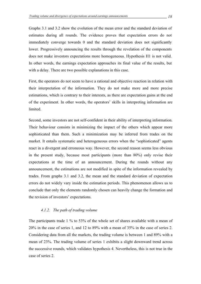
4.1.2. The path of trading volume
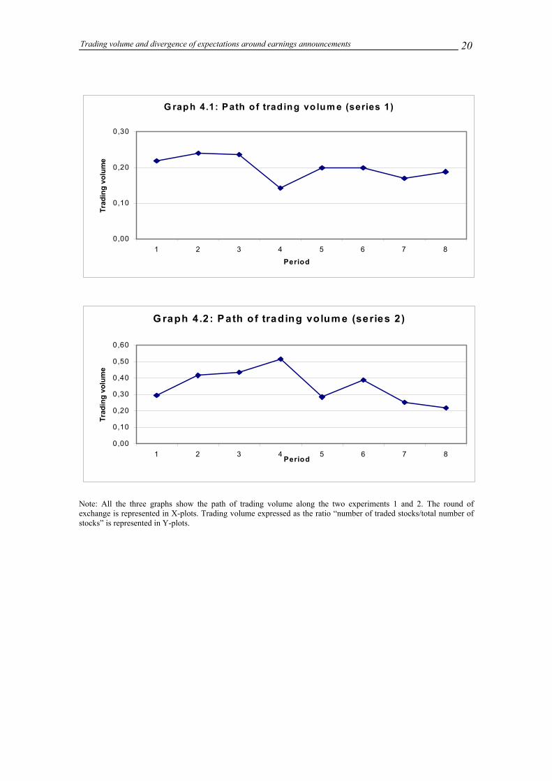
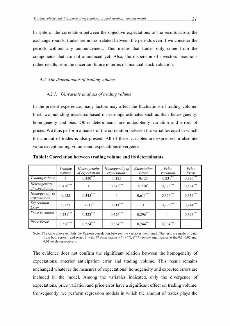
The participants trade 1 % to 53% of the whole set of shares available with a mean of
20% in the case of series 1, and 12 to 89% with a mean of 35% in the case of series 2.
Considering data from all the markets, the trading volume is between 1 and 89% with a
mean of 23%. The trading volume of series 1 exhibits a slight downward trend across
the successive rounds, which validates hypothesis 4. Nevertheless, this is not true in the
case of series 2.
Trading volume and divergence of expectations around earnings announcements 19
G raph 4: Path o f trad ing vo lum e (all data)
0 ,00
0 ,10
0 ,20
0 ,30
1 2 3 4 5 6 7 8Period
Trad
ing
volu
me
Trading volume and divergence of expectations around earnings announcements 20
G raph 4.1: Path o f trad ing volum e (series 1)
0,00
0,10
0,20
0,30
1 2 3 4 5 6 7 8
Period
Trad
ing
volu
me
G raph 4.2: Path of trading volum e (series 2)
0,00
0,10
0,20
0,30
0,40
0,50
0,60
1 2 3 4 5 6 7 8Period
Trad
ing
volu
me
Note: All the three graphs show the path of trading volume along the two experiments 1 and 2. The round of exchange is represented in X-plots. Trading volume expressed as the ratio “number of traded stocks/total number of stocks” is represented in Y-plots.
Trading volume and divergence of expectations around earnings announcements 21
In spite of the correlation between the objective expectations of the results across the
exchange rounds, trades are not correlated between the periods even if we consider the
periods without any announcement. This means that trades only come from the
components that are not announced yet. Also, the dispersion of investors’ reactions
rather results from the uncertain future in terms of financial stock valuation.
4.2. The determinants of trading volume
4.2.1. Univariate analysis of trading volume
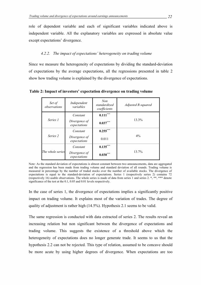
In the present experience, many factors may affect the fluctuations of trading volume.
First, we including measures based on earnings estimates such as their heterogeneity,
homogeneity and bias. Other determinants are undoubtedly variation and errors of
prices. We thus perform a matrix of the correlation between the variables cited in which
the amount of trades is also present. All of these variables are expressed in absolute
value except trading volume and expectations divergence.
Table1: Correlation between trading volume and its determinants
Trading volume
Heterogeneity of expectations
Homogeneity of expectations
Expectation Error
Price variation
Price Error
Trading volume 1 0,420*** 0,125 0,125 0,231** 0,326*** Heterogeneity of expectations 0,420*** 1 0,345*** 0,218* 0,323*** 0,524***
Homogeneity of expectations 0,125 0,345*** 1 0,611*** 0,376*** 0,334***
Expectation Error 0,125 0,218* 0,611*** 1 0,296*** 0,744***
Price variation 0,231*** 0,323*** 0,376*** 0,296*** 1 0,394***
Price Error 0,326*** 0,524*** 0,334*** 0,744*** 0,394*** 1
Note: The table above exhibits the Pearson correlation between the variables mentioned. The tests are made of data from both series 1 and series 2, with 77 observations. (*), (**), (***) denote significance at the 0.1, 0.05 and 0.01 levels respectively.
The evidence does not confirm the significant relation between the homogeneity of
expectations; anterior anticipation error and trading volume. This result remains
unchanged whatever the measures of expectations’ homogeneity and expected errors are
included in the model. Among the variables indicated, only the divergence of
expectations, price variation and price error have a significant effect on trading volume.
Consequently, we perform regression models in which the amount of trades plays the
Trading volume and divergence of expectations around earnings announcements 22
role of dependent variable and each of significant variables indicated above is
independent variable. All the explanatory variables are expressed in absolute value
except expectations’ divergence.
4.2.2. The impact of expectations’ heterogeneity on trading volume
Since we measure the heterogeneity of expectations by dividing the standard-deviation
of expectations by the average expectations, all the regressions presented in table 2
show how trading volume is explained by the divergence of expectations.
Table 2: Impact of investors’ expectation divergence on trading volume
Set of observations
Independent variables
Non standardized coefficients
Adjusted R-squared
Constant 0.111*** Series 1 Divergence of
expectations 0.037*** 13.3%
Constant 0.255*** Series 2 Divergence of
expectations 0.011 4%
Constant 0.135*** The whole series Divergence of
expectations 0.030*** 13.7%
Note: As the standard deviation of expectations is almost constant between two announcements, data are aggregated and the regression has been made from trading volume and standard deviation of all rounds. Trading volume is measured in percentage by the number of traded stocks over the number of available stocks. The divergence of expectations is equal to the standard-deviation of expectations. Series 1 (respectively series 2) contains 72 (respectively 16) usable observations. The whole series is made of data from series 1 and series 2. *, **, *** denote significance of the test at the 0.1, 0.05 and 0.01 levels respectively.
In the case of series 1, the divergence of expectations implies a significantly positive
impact on trading volume. It explains most of the variation of trades. The degree of
quality of adjustment is rather high (14.5%). Hypothesis 2.1 seems to be valid.
The same regression is conducted with data extracted of series 2. The results reveal an
increasing relation but non significant between the divergence of expectations and
trading volume. This suggests the existence of a threshold above which the
heterogeneity of expectations does no longer generate trade. It seems to us that the
hypothesis 2.2 can not be rejected. This type of relation, assumed to be concave should
be more acute by using higher degrees of divergence. When expectations are too
Trading volume and divergence of expectations around earnings announcements 23
dispersed, every investor becomes aware of this divergence due to the transparency of
the double-auction market. In these conditions, the investors become less self-confident
and place fewer orders, which lowers the level of trading volume. Sometimes, the
investors do trade without taking care about theirs expectations on the basis of other
investors’ expectations. In that case, limit orders converge, even if the level of trading is
lower.
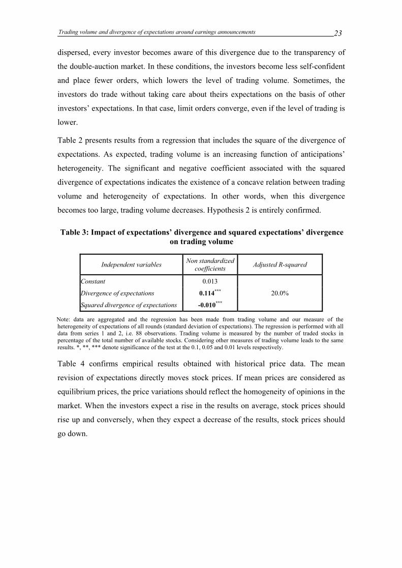
Table 2 presents results from a regression that includes the square of the divergence of
expectations. As expected, trading volume is an increasing function of anticipations’
heterogeneity. The significant and negative coefficient associated with the squared
divergence of expectations indicates the existence of a concave relation between trading
volume and heterogeneity of expectations. In other words, when this divergence
becomes too large, trading volume decreases. Hypothesis 2 is entirely confirmed.
Table 3: Impact of expectations’ divergence and squared expectations’ divergence on trading volume
Independent variables Non standardized coefficients Adjusted R-squared
Constant 0.013
Divergence of expectations 0.114*** 20.0%
Squared divergence of expectations -0.010***
Note: data are aggregated and the regression has been made from trading volume and our measure of the heterogeneity of expectations of all rounds (standard deviation of expectations). The regression is performed with all data from series 1 and 2, i.e. 88 observations. Trading volume is measured by the number of traded stocks in percentage of the total number of available stocks. Considering other measures of trading volume leads to the same results. *, **, *** denote significance of the test at the 0.1, 0.05 and 0.01 levels respectively.
Table 4 confirms empirical results obtained with historical price data. The mean
revision of expectations directly moves stock prices. If mean prices are considered as
equilibrium prices, the price variations should reflect the homogeneity of opinions in the
market. When the investors expect a rise in the results on average, stock prices should
rise up and conversely, when they expect a decrease of the results, stock prices should
go down.
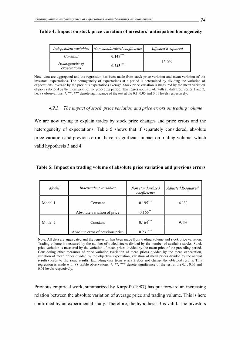
Trading volume and divergence of expectations around earnings announcements 24
Table 4: Impact on stock price variation of investors’ anticipation homogeneity
Independent variables Non standardized coefficients Adjusted R-squared
Constant 0.149***
Homogeneity of expectations 0.243***
13.0%
Note: data are aggregated and the regression has been made from stock price variation and mean variation of the investors' expectations. The homogeneity of expectations at a period is determined by dividing the variation of expectations’ average by the previous expectations average. Stock price variation is measured by the mean variation of prices divided by the mean price of the preceding period. This regression is made with all data from series 1 and 2, i.e. 88 observations. *, **, *** denote significance of the test at the 0.1, 0.05 and 0.01 levels respectively.
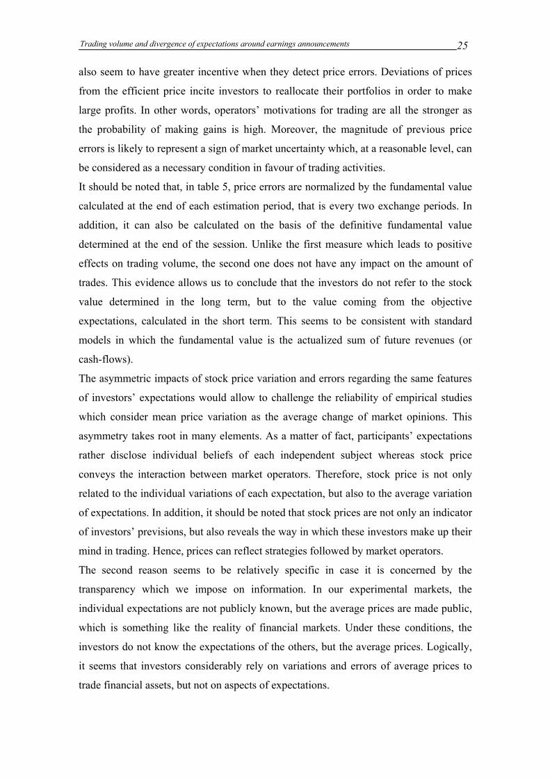
4.2.3. The impact of stock price variation and price errors on trading volume
We are now trying to explain trades by stock price changes and price errors and the
heterogeneity of expectations. Table 5 shows that if separately considered, absolute
price variation and previous errors have a significant impact on trading volume, which
valid hypothesis 3 and 4.
Table 5: Impact on trading volume of absolute price variation and previous errors
Model Independent variables Non standardized coefficients
Adjusted R-squared
Constant 0.195*** Model 1
Absolute variation of price 0.166**
4.1%
Constant 0.164*** Model 2
Absolute error of previous price 0.231***
9.4%
Note: All data are aggregated and the regression has been made from trading volume and stock price variation. Trading volume is measured by the number of traded stocks divided by the number of available stocks. Stock price variation is measured by the variation of mean prices divided by the mean price of the preceding period. Considering other measures of price variation (variation of mean prices divided by the mean expectation, variation of mean prices divided by the objective expectation, variation of mean prices divided by the annual results) leads to the same results. Excluding data from series 2 does not change the obtained results. This regression is made with 88 usable observations. *, **, *** denote significance of the test at the 0.1, 0.05 and 0.01 levels respectively.
Previous empirical work, summarized by Karpoff (1987) has put forward an increasing
relation between the absolute variation of average price and trading volume. This is here
confirmed by an experimental study. Therefore, the hypothesis 3 is valid. The investors
Trading volume and divergence of expectations around earnings announcements 25
also seem to have greater incentive when they detect price errors. Deviations of prices
from the efficient price incite investors to reallocate their portfolios in order to make
large profits. In other words, operators’ motivations for trading are all the stronger as
the probability of making gains is high. Moreover, the magnitude of previous price
errors is likely to represent a sign of market uncertainty which, at a reasonable level, can
be considered as a necessary condition in favour of trading activities.
It should be noted that, in table 5, price errors are normalized by the fundamental value
calculated at the end of each estimation period, that is every two exchange periods. In
addition, it can also be calculated on the basis of the definitive fundamental value
determined at the end of the session. Unlike the first measure which leads to positive
effects on trading volume, the second one does not have any impact on the amount of
trades. This evidence allows us to conclude that the investors do not refer to the stock
value determined in the long term, but to the value coming from the objective
expectations, calculated in the short term. This seems to be consistent with standard
models in which the fundamental value is the actualized sum of future revenues (or
cash-flows).
The asymmetric impacts of stock price variation and errors regarding the same features
of investors’ expectations would allow to challenge the reliability of empirical studies
which consider mean price variation as the average change of market opinions. This
asymmetry takes root in many elements. As a matter of fact, participants’ expectations
rather disclose individual beliefs of each independent subject whereas stock price
conveys the interaction between market operators. Therefore, stock price is not only
related to the individual variations of each expectation, but also to the average variation
of expectations. In addition, it should be noted that stock prices are not only an indicator
of investors’ previsions, but also reveals the way in which these investors make up their
mind in trading. Hence, prices can reflect strategies followed by market operators.
The second reason seems to be relatively specific in case it is concerned by the
transparency which we impose on information. In our experimental markets, the
individual expectations are not publicly known, but the average prices are made public,
which is something like the reality of financial markets. Under these conditions, the
investors do not know the expectations of the others, but the average prices. Logically,
it seems that investors considerably rely on variations and errors of average prices to
trade financial assets, but not on aspects of expectations.
Trading volume and divergence of expectations around earnings announcements 26
We now put the mean variation and errors of prices as well as the divergence of
investors’ expectations in the same regression model where trading volume is the
dependent variable. The aim of this procedure, as previously mentioned, is to justify the
dominance of one variable against the others. However, in such a model, we have to
take care of the interaction between independent variables because the existence of
strong linear dependences may distort the estimation results of model coefficients.
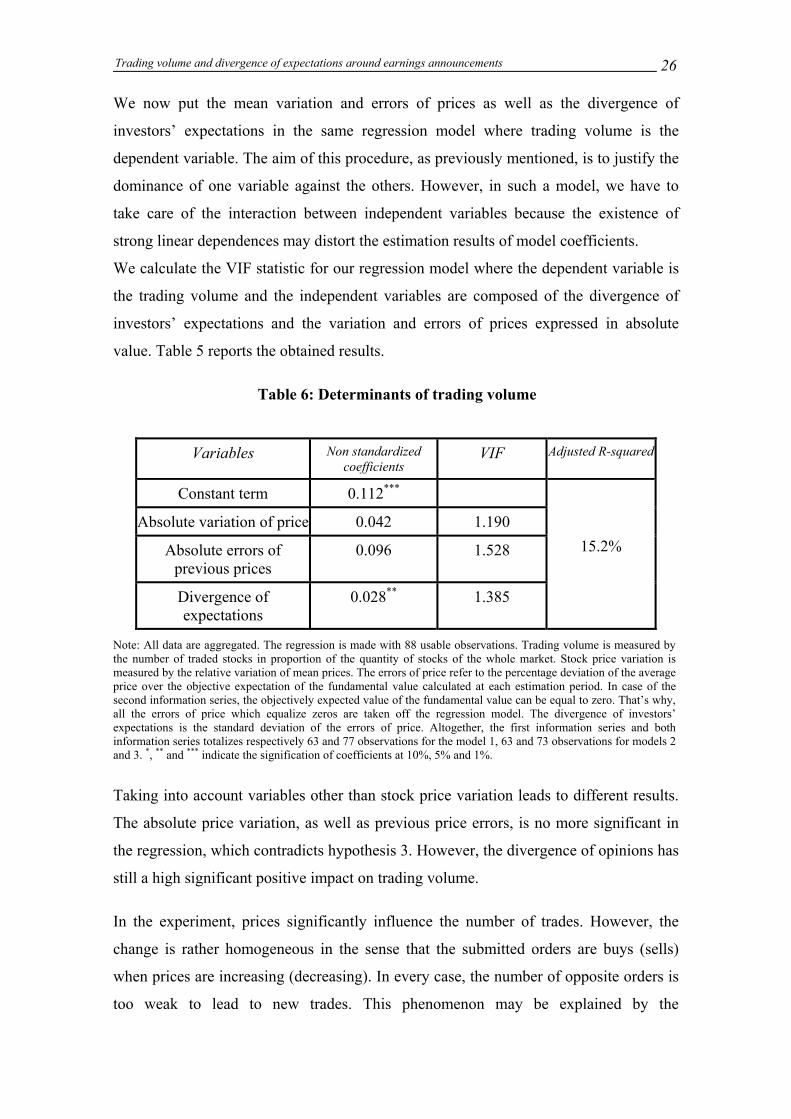
We calculate the VIF statistic for our regression model where the dependent variable is
the trading volume and the independent variables are composed of the divergence of
investors’ expectations and the variation and errors of prices expressed in absolute
value. Table 5 reports the obtained results.
Table 6: Determinants of trading volume
Variables Non standardized
coefficients VIF Adjusted R-squared
Constant term 0.112***
Absolute variation of price 0.042 1.190
Absolute errors of previous prices
0.096 1.528
Divergence of expectations
0.028** 1.385
15.2%
Note: All data are aggregated. The regression is made with 88 usable observations. Trading volume is measured by the number of traded stocks in proportion of the quantity of stocks of the whole market. Stock price variation is measured by the relative variation of mean prices. The errors of price refer to the percentage deviation of the average price over the objective expectation of the fundamental value calculated at each estimation period. In case of the second information series, the objectively expected value of the fundamental value can be equal to zero. That’s why, all the errors of price which equalize zeros are taken off the regression model. The divergence of investors’ expectations is the standard deviation of the errors of price. Altogether, the first information series and both information series totalizes respectively 63 and 77 observations for the model 1, 63 and 73 observations for models 2 and 3. *, ** and *** indicate the signification of coefficients at 10%, 5% and 1%.
Taking into account variables other than stock price variation leads to different results.
The absolute price variation, as well as previous price errors, is no more significant in
the regression, which contradicts hypothesis 3. However, the divergence of opinions has
still a high significant positive impact on trading volume.
In the experiment, prices significantly influence the number of trades. However, the
change is rather homogeneous in the sense that the submitted orders are buys (sells)
when prices are increasing (decreasing). In every case, the number of opposite orders is
too weak to lead to new trades. This phenomenon may be explained by the
Trading volume and divergence of expectations around earnings announcements 27
characteristics of the experimental markets in the sense that there are no traders entering
the market or going out of the market. This should entail that there are no new buying or
selling needs matching the existing orders. This is not the case of real markets. The
existence of new traders may explain why some empirical studies exhibit a relation
between the change in trading volume and the variation of stock prices. Only the
divergence of interpretations on the annual results has an impact on trading volume.
An increasing relation between the trading volume of this experimental market and the
heterogeneity of expectations is put forward when the divergence is not too high. On the
contrary, the divergence does not generate trading volume. A significant link has been
detected between the absolute price variation and trading volume, but this factor is a
lower determinant of trading volume compared to the divergence of opinions.
To sum-up, trading volume is different from 0 in spite of a structure of common
information for all the investors. This means that the theorem of no-trade is violated.
Moreover, this absence of no trading volume is not only due to the change in
fundamental stock value but also to the investors’ different interpretations of public
information. The latter is a major determinant of trading volume.
5. Conclusion
This paper mainly allows the role of divergence of investors’ earnings interpretations in
explaining the path of trades to be analyzed. First, the investors’ expectations remain
heterogeneous until the final diffusion in spite of successive announcements of results
components. Moreover, they do not seem to come from a rational expectations model in
absence of asymmetric information.
The heterogeneity of expectations explains a great part of the variation of trades on the
market unless it becomes too strong. As expected, trading volume is an increasing
function of the heterogeneity of expectations. Moreover, the relation between trading
volume and the divergence of opinions is concave. In other words, when the divergence
of interpretations becomes too large, trading volume decreases. Conversely, the range of
stock price variation has a lower impact on trades. This means that price level is not
leading transactions. Only the heterogeneous expectations may imply orders of opposite
sense and trades.
Trading volume and divergence of expectations around earnings announcements 28
The obtained results justify the importance of the trading volume in studies of market
reaction, especially when the abnormal returns seem insufficient to explain the
anomalies coming from the public information. As a matter of fact, this variable puts
forward the heterogeneous character of market reaction and allows to complete the
homogeneous aspect of price evolution.
From these results here, it may be wondered why the individual expectations differ from
the value that comes from a rational expectations model? Why are trading prices
different from the fundamental stock value? The answer to these questions needs the use
of the experimental method.
6. References
Atiase R.K. and L.S. Bamber, 1994, “Trading Volume Reactions to Annual Accounting
Earnings Announcements”, Journal of Accounting and Economics, 17(3), 309-329.
Bamber L.S., O.E. Barron and T.L.Stober, 1997, “Trading volume and Different
Aspects of Disagreement Coincident with Earnings Announcements”, The Accounting
Review, 72(4), 575-597.
Bamber L.S., O.E. Barron and T.L.Stober,, 1999, “Differential Interpretations and
Trading Volume”, Journal of Financial and Quantitative Analysis, 34(3), 369-386.
Gillette A.B., D.E. Stevens, S.G. Watts and A.W. Williams, 1999, “Price and volume
reaction to public information releases: an experimental approach incorporating traders’
subjective beliefs”, Contemporary Accounting Research, 16(3), 347-379.
Gode D.K. and S. Sunder, 1993, “Allocative efficiency of market with zero-intelligence
traders: market as a partial substitute for individual rationality”, Journal of Political
Economy, 101(1), 119-126.
Kandel E. and N. Pearson, 1995, “Differential Interpretation of Public Signals and
Trade in Speculative Markets”, Journal of Political Economy, 103(4), 831-872.
Trading volume and divergence of expectations around earnings announcements 29
Karpoff J.M., 1987, “The Relation between Price Changes and Trading Volume : A
Survey”, Journal of Financial and Quantitative Analysis, 22(1), 109-126.
Kim O. and R.E. Verrecchia, 1991, “Trading volume and price reactions to public
announcements”, Journal of Accounting Research, 29(2), 302-321.
Theissen E., 2000, “Market structure, informational efficiency and liquidity trading: an
experimental comparison of auction and dealer markets“, Journal of Financial Markets,
3(4), 333-363.
Ziebart D.A., 1990, “The association between consensus of beliefs and trading activity
surrounding earnings announcements”, The Accounting Review, 65(2), 477-488.
7. Annex
Instructions for the experiment
You are welcome to participate to our market which allows you to earn money. Your
gain depends on your decisions and also on others’ decisions. Each participant makes up
his/her decisions individually in front of her computer. It is strictly forbidden to
communicate with the others. It is a case of exclusion from the experiment and the
gains.
You participate to a market in which you can trade stocks in order to win money by
using the information contained in the good value. This is a market of eight rounds of
exchange with an initial endowment of 20 shares and 200 ECU (Experimental Cash
Unit). You can buy stocks to other persons with your cash or sell your stocks. The gain
issued from a sell is the difference between the selling price and the stock value.
Conversely, the gain issued from a buy is the difference between the stock value and the
buying price. The exchange gains are issued from the sum of the gains issued from buys
and sells. Therefore, they strictly depend on what you can sell your stocks above or buy
goods under the stock value.
How to determine the good value?
Trading volume and divergence of expectations around earnings announcements 30
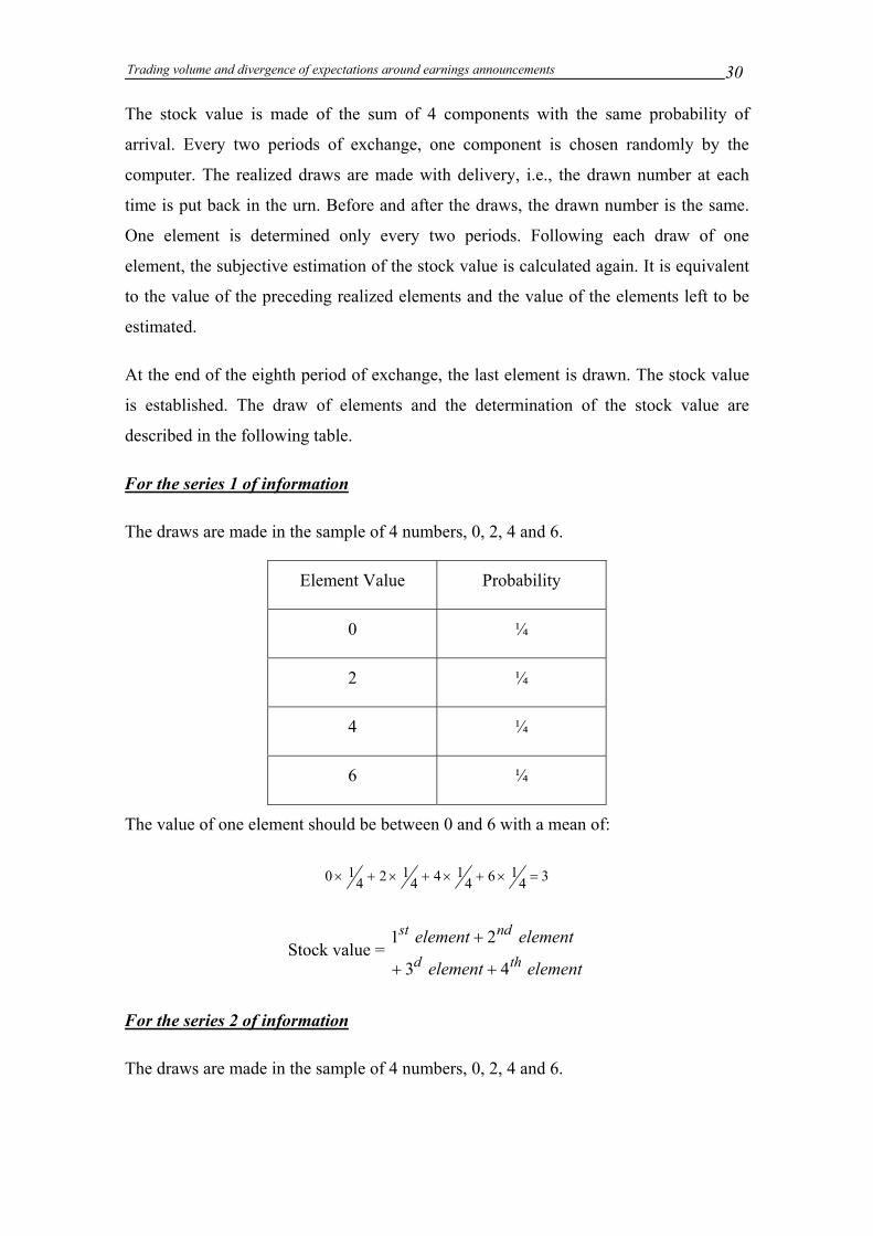
The stock value is made of the sum of 4 components with the same probability of
arrival. Every two periods of exchange, one component is chosen randomly by the
computer. The realized draws are made with delivery, i.e., the drawn number at each
time is put back in the urn. Before and after the draws, the drawn number is the same.
One element is determined only every two periods. Following each draw of one
element, the subjective estimation of the stock value is calculated again. It is equivalent
to the value of the preceding realized elements and the value of the elements left to be
estimated.
At the end of the eighth period of exchange, the last element is drawn. The stock value
is established. The draw of elements and the determination of the stock value are
described in the following table.
For the series 1 of information
The draws are made in the sample of 4 numbers, 0, 2, 4 and 6.
Element Value Probability
0 ¼
2 ¼
4 ¼
6 ¼
The value of one element should be between 0 and 6 with a mean of:
34164
144124
10 =×+×+×+×
Stock value = elementelement
elementelementthd
ndst
43
21
++
+
For the series 2 of information
The draws are made in the sample of 4 numbers, 0, 2, 4 and 6.
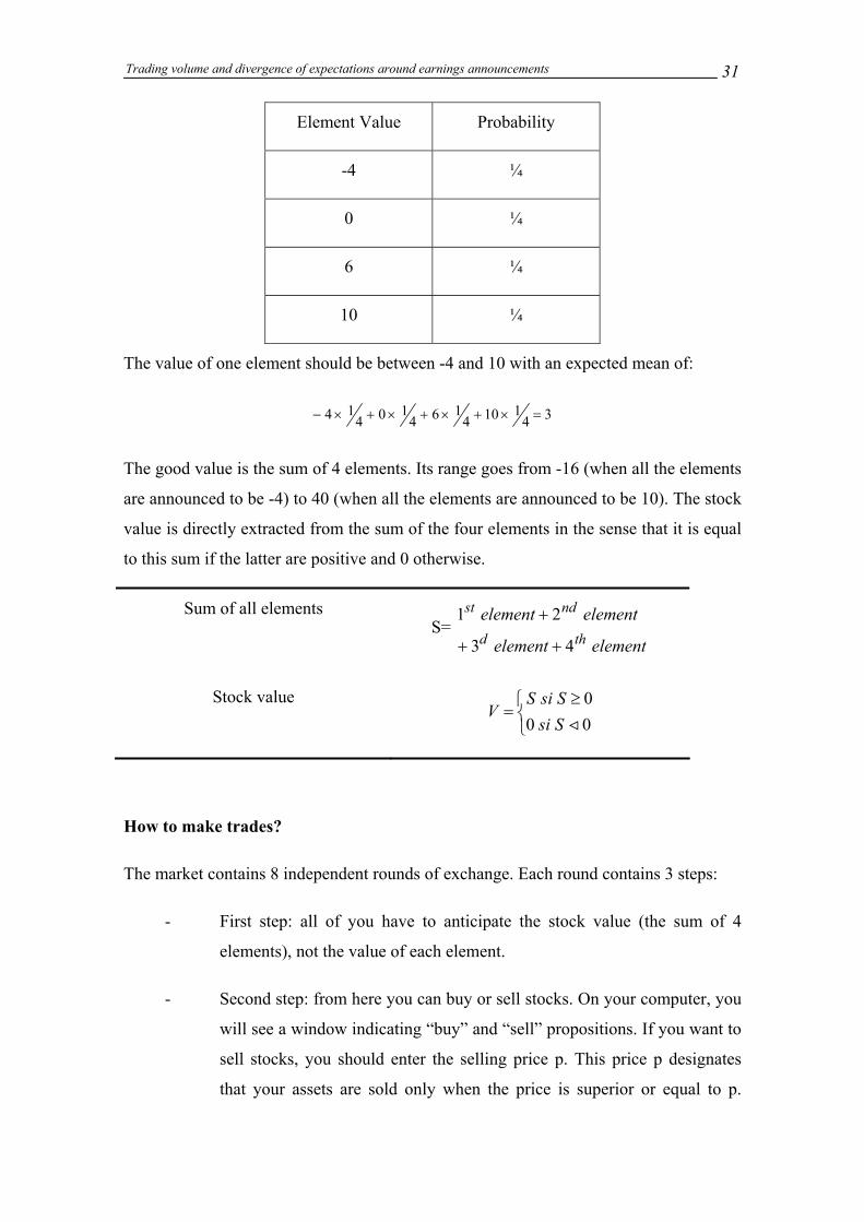
Trading volume and divergence of expectations around earnings announcements 31
Element Value Probability
-4 ¼
0 ¼
6 ¼
10 ¼
The value of one element should be between -4 and 10 with an expected mean of:
341104
164104
14 =×+×+×+×−
The good value is the sum of 4 elements. Its range goes from -16 (when all the elements
are announced to be -4) to 40 (when all the elements are announced to be 10). The stock
value is directly extracted from the sum of the four elements in the sense that it is equal
to this sum if the latter are positive and 0 otherwise.
Sum of all elements S=
elementelement
elementelementthd
ndst
43
21
++
+
Stock value
≥
=000
<SsiSsiS
V
How to make trades?
The market contains 8 independent rounds of exchange. Each round contains 3 steps:
- First step: all of you have to anticipate the stock value (the sum of 4
elements), not the value of each element.
- Second step: from here you can buy or sell stocks. On your computer, you
will see a window indicating “buy” and “sell” propositions. If you want to
sell stocks, you should enter the selling price p. This price p designates
that your assets are sold only when the price is superior or equal to p.
Trading volume and divergence of expectations around earnings announcements 32
Conversely, if you want to buy stocks, you have to enter the buying price
p. This price p designates that your stocks are bought only when the price
is inferior or equal to p. In both cases, the quantity of traded stocks is
automatically equal to 1. As a consequence, if you want to trade X stocks
(X>1), you have to submit X propositions. Your selling proposition
(respectively buying one) is always added to the list of selling
propositions (resp. buying ones) appearing on your screen. It is executed
as soon as there is one proposition which satisfies your price condition.
However, you can also execute directly a sell or a buy by clicking a
proposition on the list and button “OK”. After its execution, the
proposition is withdrawn from the equivalent list. You can make
propositions at every time from the round. The not executed propositions
can be modified or cancelled in the same period. However, the non
executed propositions from one period do not enter the list of trade
propositions of the following periods.
- Third step: this is the phase of announcement of the drawn element. A
random element is announced at the end of periods 2, 4, 6, 8 and
mentioned in box “drawn element”. At the other periods without any
announcement, the message “no element is drawn at this period” appears
in the same box.
How to calculate your gains?
At the end of the eighth period, all your remaining stocks are bought back at a price
equal to the stock value. Your final retribution contains three components. Besides an
initially fixed sum (part 1), you will receive a premium strictly linked to the accuracy of
the expectations of the stock value (part 2) and the gains linked to your trades (part 3).
The cash you win is equal to the sum of parts 1, 2 and 3, as follows:
Your retribution = Part 1 + (Part 2 + Part 3)* conversion rate
The rate of conversion is defined so that each of you earns from 10 to 30 Canadian
dollars, with a mean of 25 $CA.

Trading volume and divergence of expectations around earnings announcements 33
Please read carefully the instructions and ask questions about what you do not
understand. A great understanding will allow you to play our game in a better way.