Adaptive Pseudo Dilation for Gestalt Edge Grouping and Contour Detection
arX
iv:g
r-qc
/960
4027
v1 1
2 A
pr 1
996
An exact solution of the metric-affine gauge theory with dilation,
shear, and spin charges
Yu.N. Obukhov∗, E.J. Vlachynsky†, W. Esser, R. Tresguerres‡ and F.W. Hehl
Institute for Theoretical Physics, University of Cologne
D-50923 Koln, Germany
Abstract
The spacetime of the metric-affine gauge theory of gravity (MAG) encom-
passes nonmetricity Qαβ and torsion Tα as post-Riemannian structures. The
sources of MAG are the conserved currents of energy-momentum and dilation
⊕ shear ⊕ spin. We present an exact static spherically symmetric vacuum
solution of the theory describing the exterior of a lump of matter carrying
mass and dilation ⊕ shear ⊕ spin charges.
PACS no.: 04.50.+h; 04.20.Jb; 03.50.Kk
Typeset using REVTEX
∗Permanent address: Department of Theoretical Physics, Moscow State University, 117234
Moscow, Russia
†Permanent address: Department of Mathematics, University of Newcastle, Newcastle, NSW 2308,
Australia
‡Permanent address: Consejo Superior de Investigaciones Cientificas, Serrano 123, 28006 Madrid,
Spain
1
1. INTRODUCTION
The four-dimensional affine group A(4, R) is the semidirect product of of the translation
group R4 and the linear group GL(4, R). If one gauges the affine group and additionally
allows for a metric g, then one ends up with a gravitational theory, the metric-affine gauge
theory of gravity (‘metric-affine gravity’ MAG), see [1], the spacetime of which encompasses
two different post-Riemannian structures: the nonmetricity one-form Qαβ = Qiαβ dxi and
the torsion two-form T α = 12Tij
αdxi ∧ dxj. Gauge models in which Qαβ and T α both
provide propagating modes, that is, if they are not tied to the material sources, have, in the
Yang-Mills fashion, gauge Lagrangians quadratic in curvature, torsion, and nonmetricity:
VMAG ∼1
2κ
(R + λ + T 2 + TQ + Q2
)+ R2 . (1.1)
Here we denote Einstein’s gravitational constant by κ = ℓ2/(hc) (the Planck length is ℓ),
the cosmological constant by λ, and the curvature two-form by Rαβ = 1
2Rijα
βdxi ∧ dxj.
One way to investigate the potentialities of such models is to look for exact solutions.
Typically one starts with the Schwarzschild or the Kerr solution and tries to find a corre-
sponding generalization appropriate for the spacetime geometry under consideration. As
a first step, one requires the nonmetricity to vanish. Then the connection of spacetime is
metric-compatible and the corresponding gauge model is described by the Poincare gauge
theory (PG) residing in a Riemann-Cartan spacetime. In the framework of the PG (Q = 0),
for a Lagrangian as in (1.1), but without a linear piece R, McCrea et al., see [2], found an
electrically charged Kerr-NUT solution with torsion. Ordinary Newton-Einstein gravity is
provided in such a model by the T 2-pieces, whereas the R2-pieces supply ‘strong gravity’
with a potential increasing as r2, where r is a radial coordinate. In a similar model, but
with an external massless scalar field, Baekler et al. [3] found a torsion kink as an exact
solution. Certainly, a lot still needs to be investigated in the framework of the PG, but the
time seems ripe to turn one’s attention to full-fledged MAG.
The search for exact solutions within MAG has been pioneered by Tresguerres [4,5] and by
Tucker and Wang [6]. With propagating nonmetricity Qαβ two types of charge are expected
2
to arise: One dilation charge related to the trace Qγγ of the nonmetricity — Q := Qγ
γ/4
is called the Weyl covector — and nine types of shear charge related to the remaining
traceless piece րQαβ := Qαβ − Q gαβ of the nonmetricity. Under the local Lorentz group,
the nonmetricity can be decomposed into four irreducible pieces (I)Qαβ, with I = 1, 2, 3, 4.
It splits according to 40 = 16 ⊕ 16 ⊕ 4 ⊕ 4, see [1] p.122. The Weyl covector is linked to
(4)Qαβ = Q gαβ. Therefore we should find 4 + 4 + 1 shear charges and 1 dilation charge.
The simplest solution with nonmetricity should carry a dilation charge (which couples to
the Weyl covector Q) and should be free of shear charges. Then the gauge Lagrangian VMAG
is not needed in its full generality, rather we can restrict ourselves to (R + Q2) /2κ + R2 or,
more exactly [7,8,6], with constants α and β, to
Vdil = −1
2κ
(Rαβ ∧ ηαβ + β Q ∧ ∗Q
)−
α
8Rα
α ∧ ∗Rββ . (1.2)
Here ηαβ := ∗(ϑα ∧ ϑβ), where ϑγ denotes the coframe, and the star is the Hodge opera-
tor. Observe that from the nonmetricity only the Weyl covector Q enters explicitly this
Lagrangian. The last term in (1.2) is proportional to the square of Weyl’s segmental curva-
ture, Rαα = 2d Q. This is a sheer post-Riemannian piece that would vanish identically in
any Riemannian spacetime.
For β = 0, Tresguerres [4] found an exact dilation solution which has a Reissner-
Nordstrom metric, where the electric charge is substituted by the dilation charge, a Weyl
covector ∼ 1/r, and a (constrained) torsion trace proportional to the Weyl covector. Tucker
and Wang [6] confirmed this result independently. Later we will recover this dilation solution
as a specific subcase of our new solution.
The next step would then be to put on a proper shear charge, at least one of the nine
possible ones. From the point of view of the irreducible decomposition of Qαβ , the next
simple thing, beyond (4)Qαβ = Q gαβ, is to pick the vector piece (3)Qαβ , corresponding
to one shear charge. We could now amend the Lagrangian (1.2) with terms of the type
Qαβ ∧ ∗(3)Qαβ , but it is more effective to turn immediately to a more general case.
3
2. GENERAL QUADRATIC MAG-LAGRANGIAN
In a metric-affine space, the curvature has eleven irreducible pieces, see [1], Table 4. If
we recall that the nonmetricity has four and the torsion three irreducible pieces (loc.cit.),
then a general quadratic Lagrangian in MAG reads (signature − + ++):
VMAG =1
2κ
[−a0 Rαβ ∧ ηαβ − 2λ η + T α ∧ ∗
(3∑
I=1
aI(I)Tα
)
+ 2
(4∑
I=2
cI(I)Qαβ
)∧ ϑα ∧ ∗T β + Qαβ ∧ ∗
(4∑
I=1
bI(I)Qαβ
)]
−1
2Rαβ ∧ ∗
(6∑
I=1
wI(I)Wαβ +
5∑
I=1
zI(I)Zαβ
). (2.1)
In the above η := ∗1 is the volume four-form and the constants a0, · · ·a3, b1, · · · b4, c2, c3, c4,
w1, · · ·w6, z1, · · · z5 are dimensionless. In the curvature square term we have introduced
the irreducible pieces of the antisymmetric part Wαβ := R[αβ] and the symmetric part
Zαβ := R(αβ) of the curvature two-form. Again, in Zαβ, we meet a purely post-Riemannian
part. The segmental curvature is (4)Zαβ := Rγγ gαβ/4. In spite of this overabundance of
generality, it was possible [4,5] to find shear type solutions belonging to (2.1), a search
which we will continue in this work.
To begin with, let us recall the three general field equations of MAG, see [1] Eqs.(5.5.3)–
(5.5.5). Because of its redundancy, we omit the zeroth field equation with its gauge momen-
tum Mαβ . The first and the second field equations read
DHα − Eα = Σα , (2.2)
DHαβ − Eα
β = ∆αβ , (2.3)
where Σα and ∆αβ are the canonical energy-momentum and hypermomentum current three-
forms associated with matter. We will consider the vacuum case with Σα = ∆αβ = 0. The
left hand sides of (2.2)–(2.3) involve the gravitational gauge field momenta two-forms Hα
and Hαβ (‘excitations’). We find them, together with Mαβ , by partial differentiation of the
Lagrangian (2.1) (T := eα⌋Tα , eα is the frame):
4
Mαβ := −2∂VMAG
∂Qαβ
= −2
κ
[∗
(4∑
I=1
bI(I)Qαβ
)
+c2 ϑ(α ∧ ∗(1)T β) + c3 ϑ(α ∧ ∗(2)T β) +1
4(c3 − c4) gαβ∗T
], (2.4)
Hα := −∂VMAG
∂T α= −
1
κ∗
[(3∑
I=1
aI(I)Tα
)+
(4∑
I=2
cI(I)Qαβ ∧ ϑβ
)], (2.5)
Hαβ := −
∂VMAG
∂Rαβ
=a0
2κηα
β + Wαβ + Zα
β, (2.6)
where we introduced the abbreviations
Wαβ := ∗
(6∑
I=1
wI(I)Wαβ
), Zαβ := ∗
(5∑
I=1
zI(I)Zαβ
). (2.7)
Finally, the three-forms Eα and Eαβ describe the canonical energy-momentum and hy-
permomentum currents of the gauge fields themselves. One can write them as follows [1]:
Eα = eα⌋VMAG + (eα⌋Tβ) ∧ Hβ + (eα⌋Rβ
γ) ∧ Hβγ +
1
2(eα⌋Qβγ)M
βγ , (2.8)
Eαβ = −ϑα ∧ Hβ − Mα
β. (2.9)
3. A SPHERICALLY SYMMETRIC FIELD CONFIGURATION
We take spherical polar coordinates (t, r, θ, φ) and choose a coframe of Schwarzschild
type
ϑ0 = f d t , ϑ1 =1
fd r , ϑ2 = r d θ , ϑ3 = r sin θ d φ , (3.1)
with an unknown function f(r). The coframe is assumed to be orthonormal, that is, with
the local Minkowski metric oαβ := diag(−1, 1, 1, 1) = oαβ, we have the special spherically
symmetric metric
ds2 = oαβ ϑα ⊗ ϑβ = −f 2 dt2 +dr2
f 2+ r2
(dθ2 + sin2 θ dφ2
). (3.2)
As for the torsion and nonmetricity configurations, we concentrate on the simplest non-
trivial case with shear. According to its irreducible decomposition (see the Appendix B of
5
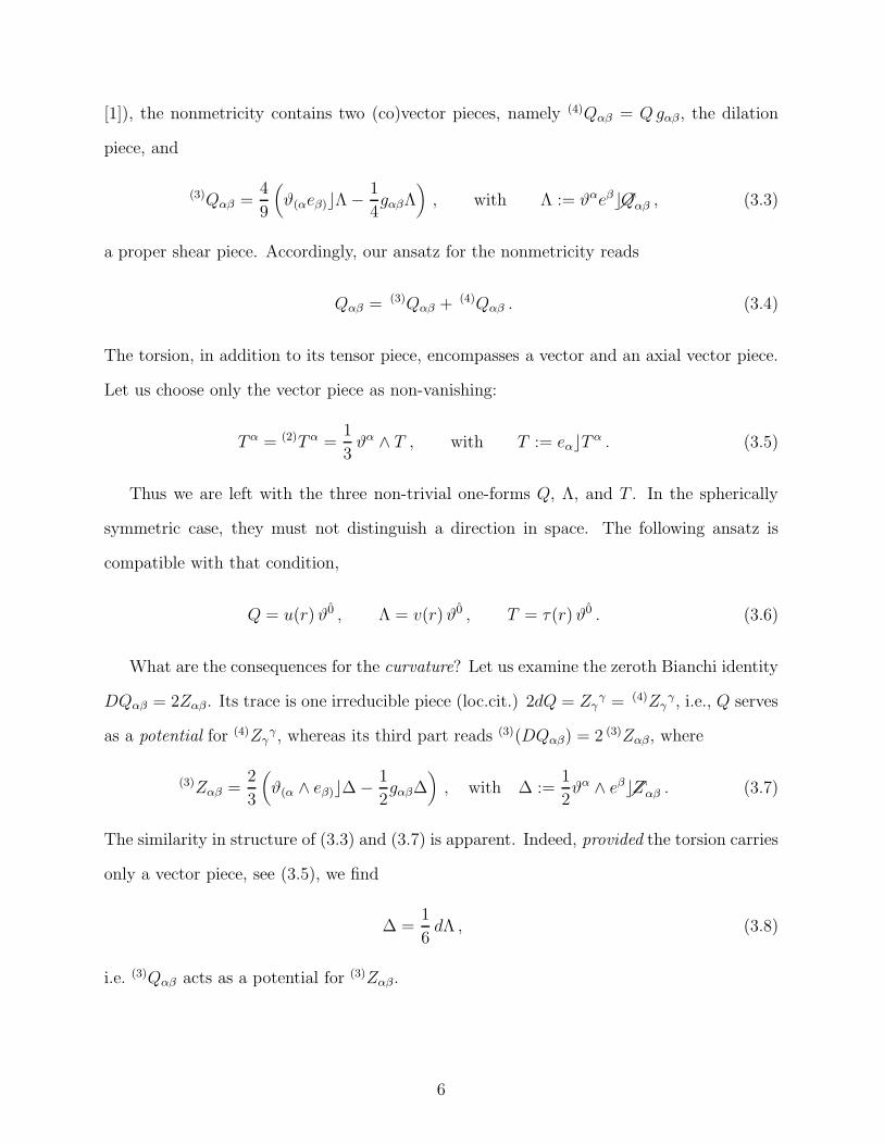
[1]), the nonmetricity contains two (co)vector pieces, namely (4)Qαβ = Q gαβ, the dilation
piece, and
(3)Qαβ =4
9
(ϑ(αeβ)⌋Λ −
1
4gαβΛ
), with Λ := ϑαeβ⌋րQαβ , (3.3)
a proper shear piece. Accordingly, our ansatz for the nonmetricity reads
Qαβ = (3)Qαβ + (4)Qαβ . (3.4)
The torsion, in addition to its tensor piece, encompasses a vector and an axial vector piece.
Let us choose only the vector piece as non-vanishing:
T α = (2)T α =1
3ϑα ∧ T , with T := eα⌋T
α . (3.5)
Thus we are left with the three non-trivial one-forms Q, Λ, and T . In the spherically
symmetric case, they must not distinguish a direction in space. The following ansatz is
compatible with that condition,
Q = u(r) ϑ0 , Λ = v(r) ϑ0 , T = τ(r) ϑ0 . (3.6)
What are the consequences for the curvature? Let us examine the zeroth Bianchi identity
DQαβ = 2Zαβ. Its trace is one irreducible piece (loc.cit.) 2dQ = Zγγ = (4)Zγ
γ, i.e., Q serves
as a potential for (4)Zγγ, whereas its third part reads (3)(DQαβ) = 2 (3)Zαβ, where
(3)Zαβ =2
3
(ϑ(α ∧ eβ)⌋∆ −
1
2gαβ∆
), with ∆ :=
1
2ϑα ∧ eβ⌋րZαβ . (3.7)
The similarity in structure of (3.3) and (3.7) is apparent. Indeed, provided the torsion carries
only a vector piece, see (3.5), we find
∆ =1
6dΛ , (3.8)
i.e. (3)Qαβ acts as a potential for (3)Zαβ.
6
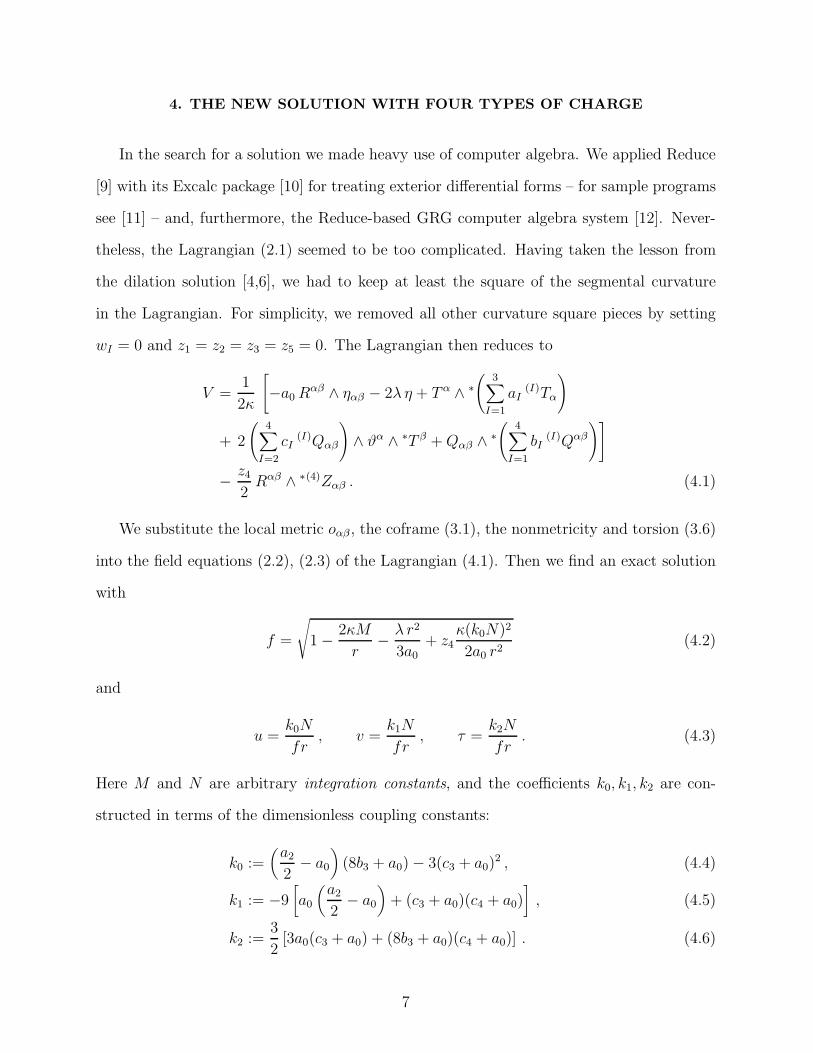
4. THE NEW SOLUTION WITH FOUR TYPES OF CHARGE
In the search for a solution we made heavy use of computer algebra. We applied Reduce
[9] with its Excalc package [10] for treating exterior differential forms – for sample programs
see [11] – and, furthermore, the Reduce-based GRG computer algebra system [12]. Never-
theless, the Lagrangian (2.1) seemed to be too complicated. Having taken the lesson from
the dilation solution [4,6], we had to keep at least the square of the segmental curvature
in the Lagrangian. For simplicity, we removed all other curvature square pieces by setting
wI = 0 and z1 = z2 = z3 = z5 = 0. The Lagrangian then reduces to
V =1
2κ
[−a0 Rαβ ∧ ηαβ − 2λ η + T α ∧ ∗
(3∑
I=1
aI(I)Tα
)
+ 2
(4∑
I=2
cI(I)Qαβ
)∧ ϑα ∧ ∗T β + Qαβ ∧ ∗
(4∑
I=1
bI(I)Qαβ
)]
−z4
2Rαβ ∧ ∗(4)Zαβ . (4.1)
We substitute the local metric oαβ , the coframe (3.1), the nonmetricity and torsion (3.6)
into the field equations (2.2), (2.3) of the Lagrangian (4.1). Then we find an exact solution
with
f =
√
1 −2κM
r−
λ r2
3a0+ z4
κ(k0N)2
2a0 r2(4.2)
and
u =k0N
fr, v =
k1N
fr, τ =
k2N
fr. (4.3)
Here M and N are arbitrary integration constants, and the coefficients k0, k1, k2 are con-
structed in terms of the dimensionless coupling constants:
k0 :=(
a2
2− a0
)(8b3 + a0) − 3(c3 + a0)
2 , (4.4)
k1 := −9[a0
(a2
2− a0
)+ (c3 + a0)(c4 + a0)
], (4.5)
k2 :=3
2[3a0(c3 + a0) + (8b3 + a0)(c4 + a0)] . (4.6)
7
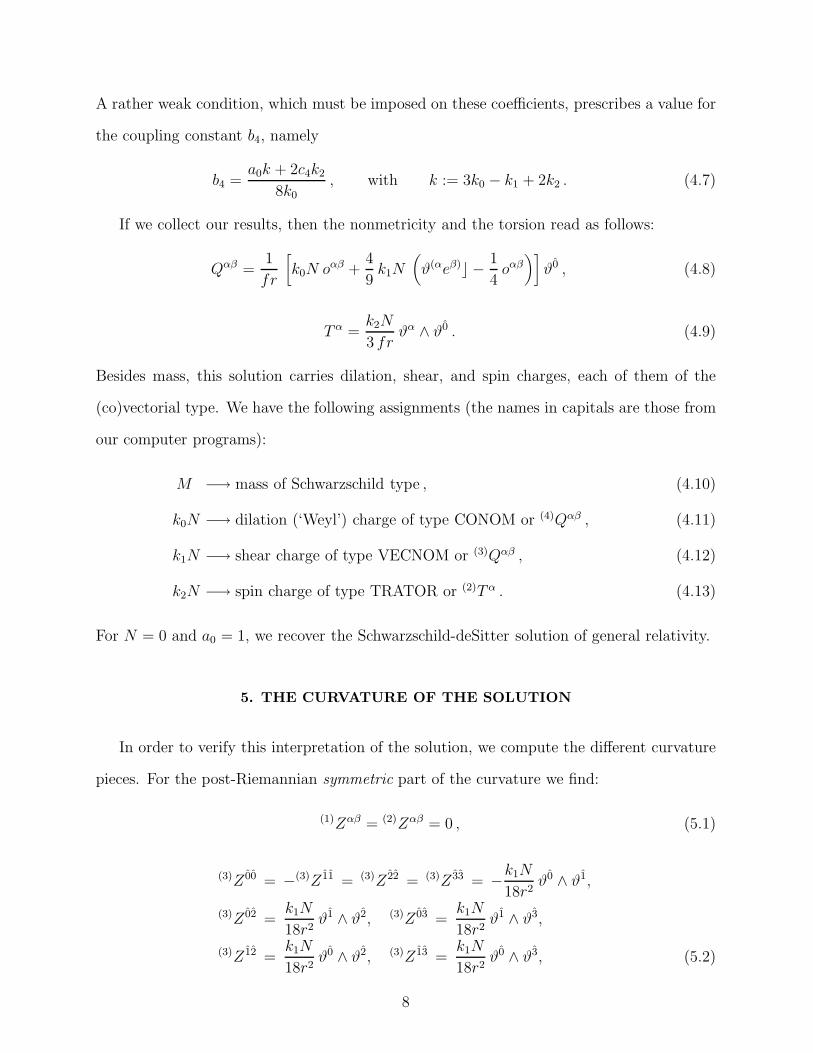
A rather weak condition, which must be imposed on these coefficients, prescribes a value for
the coupling constant b4, namely
b4 =a0k + 2c4k2
8k0, with k := 3k0 − k1 + 2k2 . (4.7)
If we collect our results, then the nonmetricity and the torsion read as follows:
Qαβ =1
fr
[k0N oαβ +
4
9k1N
(ϑ(αeβ)⌋ −
1
4oαβ
)]ϑ0 , (4.8)
T α =k2N
3 frϑα ∧ ϑ0 . (4.9)
Besides mass, this solution carries dilation, shear, and spin charges, each of them of the
(co)vectorial type. We have the following assignments (the names in capitals are those from
our computer programs):
M −→ mass of Schwarzschild type , (4.10)
k0N −→ dilation (‘Weyl’) charge of type CONOM or (4)Qαβ , (4.11)
k1N −→ shear charge of type VECNOM or (3)Qαβ , (4.12)
k2N −→ spin charge of type TRATOR or (2)T α . (4.13)
For N = 0 and a0 = 1, we recover the Schwarzschild-deSitter solution of general relativity.
5. THE CURVATURE OF THE SOLUTION
In order to verify this interpretation of the solution, we compute the different curvature
pieces. For the post-Riemannian symmetric part of the curvature we find:
(1)Zαβ = (2)Zαβ = 0 , (5.1)
(3)Z 00 = −(3)Z 11 = (3)Z 22 = (3)Z 33 = −k1N
18r2ϑ0 ∧ ϑ1,
(3)Z 02 =k1N
18r2ϑ1 ∧ ϑ2, (3)Z 03 =
k1N
18r2ϑ1 ∧ ϑ3,
(3)Z 12 =k1N
18r2ϑ0 ∧ ϑ2, (3)Z 13 =
k1N
18r2ϑ0 ∧ ϑ3, (5.2)
8
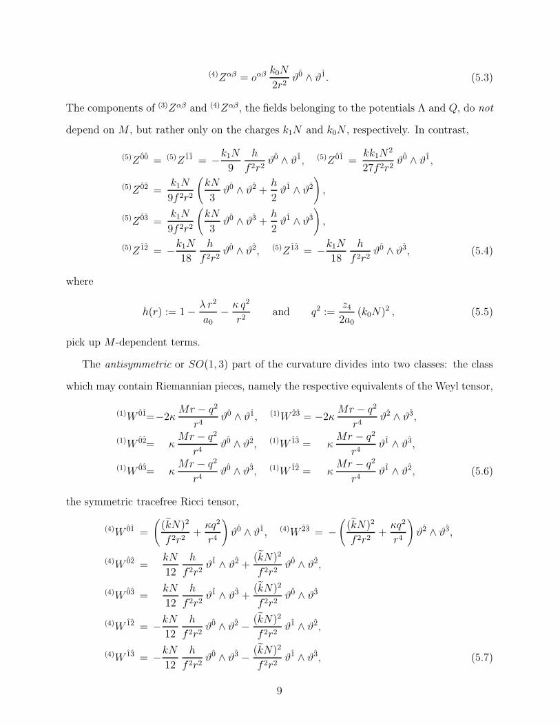
(4)Zαβ = oαβ k0N
2r2ϑ0 ∧ ϑ1. (5.3)
The components of (3)Zαβ and (4)Zαβ, the fields belonging to the potentials Λ and Q, do not
depend on M , but rather only on the charges k1N and k0N , respectively. In contrast,
(5)Z 00 = (5)Z 11 = −k1N
9
h
f 2r2ϑ0 ∧ ϑ1, (5)Z 01 =
kk1N2
27f 2r2ϑ0 ∧ ϑ1,
(5)Z 02 =k1N
9f 2r2
(kN
3ϑ0 ∧ ϑ2 +
h
2ϑ1 ∧ ϑ2
),
(5)Z 03 =k1N
9f 2r2
(kN
3ϑ0 ∧ ϑ3 +
h
2ϑ1 ∧ ϑ3
),
(5)Z 12 = −k1N
18
h
f 2r2ϑ0 ∧ ϑ2, (5)Z 13 = −
k1N
18
h
f 2r2ϑ0 ∧ ϑ3, (5.4)
where
h(r) := 1 −λ r2
a0
−κ q2
r2and q2 :=
z4
2a0
(k0N)2 , (5.5)
pick up M-dependent terms.
The antisymmetric or SO(1, 3) part of the curvature divides into two classes: the class
which may contain Riemannian pieces, namely the respective equivalents of the Weyl tensor,
(1)W 01=−2κMr − q2
r4ϑ0 ∧ ϑ1, (1)W 23 = −2κ
Mr − q2
r4ϑ2 ∧ ϑ3,
(1)W 02= κMr − q2
r4ϑ0 ∧ ϑ2, (1)W 13 = κ
Mr − q2
r4ϑ1 ∧ ϑ3,
(1)W 03= κMr − q2
r4ϑ0 ∧ ϑ3, (1)W 12 = κ
Mr − q2
r4ϑ1 ∧ ϑ2, (5.6)
the symmetric tracefree Ricci tensor,
(4)W 01 =
((kN)2
f 2r2+
κq2
r4
)ϑ0 ∧ ϑ1, (4)W 23 = −
((kN)2
f 2r2+
κq2
r4
)ϑ2 ∧ ϑ3,
(4)W 02 =kN
12
h
f 2r2ϑ1 ∧ ϑ2 +
(kN)2
f 2r2ϑ0 ∧ ϑ2,
(4)W 03 =kN
12
h
f 2r2ϑ1 ∧ ϑ3 +
(kN)2
f 2r2ϑ0 ∧ ϑ3
(4)W 12 = −kN
12
h
f 2r2ϑ0 ∧ ϑ2 −
(kN)2
f 2r2ϑ1 ∧ ϑ2,
(4)W 13 = −kN
12
h
f 2r2ϑ0 ∧ ϑ3 −
(kN)2
f 2r2ϑ1 ∧ ϑ3, (5.7)
9
where k2 := 1648
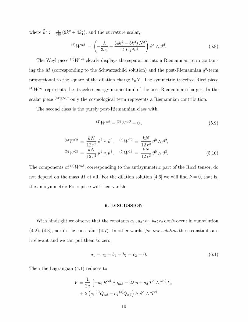
(9k2 + 4k21), and the curvature scalar,
(6)W αβ =
(−
λ
3a0+
(4k21 − 3k2) N2
216 f 2r2
)ϑα ∧ ϑβ. (5.8)
The Weyl piece (1)W αβ clearly displays the separation into a Riemannian term contain-
ing the M (corresponding to the Schwarzschild solution) and the post-Riemannian q2-term
proportional to the square of the dilation charge k0N . The symmetric tracefree Ricci piece
(4)W αβ represents the ‘traceless energy-momentum’ of the post-Riemannian charges. In the
scalar piece (6)W αβ only the cosmological term represents a Riemannian contribution.
The second class is the purely post-Riemannian class with
(2)W αβ = (3)W αβ = 0 , (5.9)
(5)W 02 =kN
12 r2ϑ1 ∧ ϑ2, (5)W 12 =
kN
12 r2ϑ0 ∧ ϑ2,
(5)W 03 =kN
12 r2ϑ1 ∧ ϑ3, (5)W 13 =
kN
12 r2ϑ0 ∧ ϑ3. (5.10)
The components of (5)W αβ, corresponding to the antisymmetric part of the Ricci tensor, do
not depend on the mass M at all. For the dilation solution [4,6] we will find k = 0, that is,
the antisymmetric Ricci piece will then vanish.
6. DISCUSSION
With hindsight we observe that the constants a1 , a3 ; b1 , b2 ; c2 don’t occur in our solution
(4.2), (4.3), nor in the constraint (4.7). In other words, for our solution these constants are
irrelevant and we can put them to zero,
a1 = a3 = b1 = b2 = c2 = 0. (6.1)
Then the Lagrangian (4.1) reduces to
V =1
2κ
[−a0 Rαβ ∧ ηαβ − 2λ η + a2 T α ∧ ∗(2)Tα
+ 2(c3
(3)Qαβ + c4(4)Qαβ
)∧ ϑα ∧ ∗T β
10
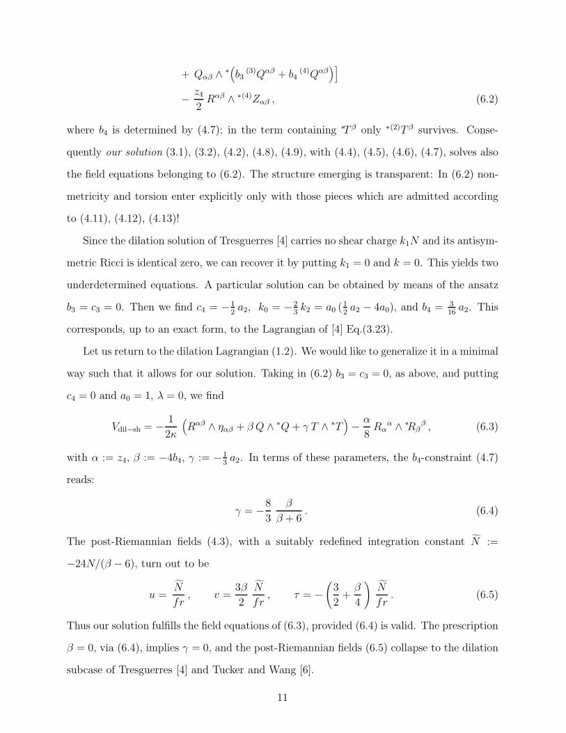
+ Qαβ ∧ ∗(b3
(3)Qαβ + b4(4)Qαβ
)]
−z4
2Rαβ ∧ ∗(4)Zαβ , (6.2)
where b4 is determined by (4.7); in the term containing ∗T β only ∗(2)T β survives. Conse-
quently our solution (3.1), (3.2), (4.2), (4.8), (4.9), with (4.4), (4.5), (4.6), (4.7), solves also
the field equations belonging to (6.2). The structure emerging is transparent: In (6.2) non-
metricity and torsion enter explicitly only with those pieces which are admitted according
to (4.11), (4.12), (4.13)!
Since the dilation solution of Tresguerres [4] carries no shear charge k1N and its antisym-
metric Ricci is identical zero, we can recover it by putting k1 = 0 and k = 0. This yields two
underdetermined equations. A particular solution can be obtained by means of the ansatz
b3 = c3 = 0. Then we find c4 = −12a2, k0 = −2
3k2 = a0 (1
2a2 − 4a0), and b4 = 3
16a2. This
corresponds, up to an exact form, to the Lagrangian of [4] Eq.(3.23).
Let us return to the dilation Lagrangian (1.2). We would like to generalize it in a minimal
way such that it allows for our solution. Taking in (6.2) b3 = c3 = 0, as above, and putting
c4 = 0 and a0 = 1, λ = 0, we find
Vdil−sh = −1
2κ
(Rαβ ∧ ηαβ + β Q ∧ ∗Q + γ T ∧ ∗T
)−
α
8Rα
α ∧ ∗Rββ , (6.3)
with α := z4, β := −4b4, γ := −13a2. In terms of these parameters, the b4-constraint (4.7)
reads:
γ = −8
3
β
β + 6. (6.4)
The post-Riemannian fields (4.3), with a suitably redefined integration constant N :=
−24N/(β − 6), turn out to be
u =N
fr, v =
3β
2
N
fr, τ = −
(3
2+
β
4
)N
fr. (6.5)
Thus our solution fulfills the field equations of (6.3), provided (6.4) is valid. The prescription
β = 0, via (6.4), implies γ = 0, and the post-Riemannian fields (6.5) collapse to the dilation
subcase of Tresguerres [4] and Tucker and Wang [6].
11
If, instead of a Reissner-Nordstrom type ansatz, we started with one using the Kerr-
NUT-Newman solution, then we would be able to find axially symmetric solutions carrying
nonmetricity and torsion. However, we will leave that to a subsequent publication.
Acknowledgments This research was supported by the Deutsche Forschungsgemeinschaft
(Bonn) under project He-528/17-1 and by the Graduate College “Scientific Computing”
(Cologne-St.Augustin).
12
REFERENCES
[1] F.W. Hehl, J.D. McCrea, E.W. Mielke, and Y. Ne’eman, Phys. Rep. 258 (1995) 1.
[2] P. Baekler, M. Gurses, F.W. Hehl, and J.D. McCrea, Phys. Lett. A128 (1988) 245.
[3] P. Baekler, E.W. Mielke, R. Hecht, and F.W. Hehl, Nucl. Phys. B288 (1987) 800.
[4] R. Tresguerres, Z. Phys. C65 (1995) 347.
[5] R. Tresguerres, Phys. Lett. A200 (1995) 405.
[6] R.W. Tucker and C. Wang, Class. Quantum Grav. 12 (1995) 2587.
[7] F.W. Hehl, E.A. Lord, and L.L. Smalley, Gen. Relat. Grav. 13 (1981) 1037.
[8] V.N. Ponomariov and Yu. Obukhov, Gen. Relat. Grav. 14 (1982) 309.
[9] A.C. Hearn, REDUCE User’s Manual. Version 3.6. Rand publication CP78 (Rev. 7/95)
(RAND, Santa Monica, CA 90407-2138, USA, 1995).
[10] E. Schrufer, F.W. Hehl, and J.D. McCrea, Gen. Relat. Grav. 19 (1987) 197.
[11] D. Stauffer, F.W. Hehl, N. Ito, V. Winkelmann, and J.G. Zabolitzky: Computer Simu-
lation and Computer Algebra – Lectures for Beginners. 3rd ed. (Springer, Berlin, 1993).
[12] V.V. Zhytnikov, GRG. Computer Algebra System for Differential Geometry, Gravity
and Field Theory. Version 3.1 (Moscow, 1991) 108 pages.
13
Copyright © 2022 FDOKUMEN