39th Congress of the European Regional Science Association 23-27 August 1999, Dublin

AN ESTIMATION OF DISPOSABLE PERSONAL INCOME OF THE SPANISH MUNICIPALITIES IN 1997

Coro Chasco Yrigoyen

Lawrence R. Klein Institute, Department of Applied Economy Autónoma University of Madrid, 28048 Madrid (Spain)

E-mail addresses:

coro.chasco@uam.es

Abstract Since 1992, Lawrence R. Klein Institute –Autónoma University of Madrid- estimates the disposable income of the Spanish municipalities, recently published in the ‘Anuario Comercial de España’ –Spanish Trade Yearbook- as scaled levels. Municipal personal income has been considered as one of the most important economic indicators, very used in a wide range of studies concerned with regional convergence, welfare analysis, marketing targets, etc. This kind of estimation can be carried out by both direct and indirect methodology. The first proceeding requires a huge information database generally difficult to obtain and not always precise, which main defect is that it cannot reflect the underground economy of Spanish municipalities. That is why direct methodology always has needed the help of indirect proceedings. These last ones find out the statistical relation of the personal disposable income and a group of socio-economic indicators for all the geographic units considered, municipalities, provinces, regions, countries, etc. In this paper, the authors present some of the indirect methods used to estimate the disposable income of Spanish municipalities. Especially the Klein estimation combines some multivariate analysis –panel data, factor and cross-section regression analysis- with a big database of almost 200 socio-economic indicators. The final estimation of the 8.099 municipalities disposable income allows us to acquire a better knowing of Spanish micro-territorial development.

1. INTRODUCTION Since 1992, Lawrence R. Klein Institute –Autónoma University of Madrid- estimates the disposable income of the Spanish municipalities. These data have been published, ranged in levels, in the ‘Atlas Comercial de España 1994’ –Spanish Trade Atlas- and recently in the ‘Anuario Comercial de España 1999’ –Spanish Trade Yearbook- sponsored by ‘la Caixa’ –the Barcelona Pensions and Savings Bank. Local personal income has been considered as one of the most important economic indicators, very used in a wide range of studies concerned with regional convergence, welfare analysis, marketing targets, etc. This kind of estimation can be carried out by both direct and indirect methodology. The first proceeding calculates the disposable income directly, considering a production function and sectorial employment matrices with municipality data. It is a complex method that requires a huge information database generally difficult to obtain and not always precise. Its main defect is that it cannot reflect the underground economy of Spanish municipalities, even when estimating agricultural gross added value (GAV). That is why direct methodology always has needed the help of indirect proceedings. These last ones find out the statistical relation of the personal disposable income and a group of socio-economic indicators for all the geographic units considered, municipalities, provinces, regions, countries, etc. This methodology, usually based in multivariate analysis, has been used by several institutions because of its capacity to detect underground economy without requiring the excessively arduous proceedings of direct method. In this paper, the authors explain some of the indirect methods used to estimate the disposable income of Spanish municipalities (Section 2); especially, Klein estimation combines some multivariate analysis with official data and own estimations (Figure 1). In Section 3, we present the selection process of some socio-economic indicators, from a big database of 130 variables related with the personal disposable income, which will be included in a panel data model. This model allows us to forecast the provincial personal disposable income, published by the INE –Spanish Institute for Statistics- with a two-year outlook. In the third chapter, a cross-section multiple regression allows us to obtain the final estimation of the municipal disposable income, taking account a set of 66 explicative variables, available for the 8.099 Spanish municipalities, and some spatial effects. In both steps, factor analysis is needed to reduce the initial explicative variables to a few uncorrelated factors.

Figure 1: The Klein estimation process of the disposable personal income for the 8.099 Spanish municipalities (1997)

Source: Chasco and Vicéns (1998).

130 socio-economic indicators . Level: provincial (50) . Period: 1986-95 (10)

Factor analysis

PROVINCIAL FORECASTING

(1997)

Provincial disposable personal income estimation, 1997

MUNICIPAL ESTIMATION

(1997)

Exogenous: 7 factors

Endogenous: disposable income

Panel-Data (‘Pool’) estimation . Level: provincial (50) . Period: 1986-95 (10)

66 socio-economic indicators database . Level: provincial (50) and municipal (8.099) . Period: 1997 (1)

Factor analysis

Exogenous: 7 factors

Endogenous: disposable income

Disposable income (INE data) . Level: provincial (50) . Period: 1986-95 (10)

Cross-section regression . Level: provincial (50)

Municipal disposable personal income estimation, 1997

2. SOME METHODOLOGICAL QUESTIONS As it has been indicated, indirect estimations of local disposable income have been used by several institutions because of its capacity to detect underground economy without requiring the excessively arduous procedures of direct method. Though municipal level approximation is always difficult, the increasingly needs of micro-data have boosted such kind of estimations during the last years. Most indirect methodologies are made up of the following scheme:

1. Selection of one/several model/s, normally the multiple regression analysis. 2. Use of the regional/provincia l income data1 as an endogenous variable in the

model. 3. Selection of some exogenous variables related with the disposable income,

available for the municipal level2. That has been the case of the Banesto estimations (1993), which used the BBV provincial data (1997)3, and of another municipal estimations made by regional institutions only for their particular municipalities, Sadei (1994) in Asturias, the Seville Deputation (1995) and the Community of Madrid Institute for Statistics (1998).

It is also necessary to highlight the contributions of some lecturers that have also estimated the municipal income of their respective regions, J. Arcarons (1994) in Catalonia, J. Esteban (1992) in the Valencia Community, C. Fernández (1992) in La Rioja, A. de las Heras (1992, 1998) in Cantabria and L. Herrero (1998) in Castile and Leon. Some of them have introduced more complex estimation methods, such as multivariate factor and cluster analysis or econometric multiequational models. Nevertheless, almost the majority have used a limited set of explicative variables –in the extreme position, the Seville Deputation only include the domestic electric power consumption variable. We must also warn about some bias due to the consideration, as almost the unique variable, of data derived from the personal income tax –IRPF in Spain- as is the case of Arcarons, in Catalonia, and the Madrid Institute for Statistics. Personal income tax still does not consider the underground economy, what is an important handicap in countries like Spain. On the contrary, indirect method takes account better the real income of families through consumption, saving and production indicators.

The main newness contributed by Klein Institute estimation process could be summarised in the following items (Chasco and Vicéns, 1998):

1 The most usual statistic fonts for provincial income are BBV –Bilbao Biscay Bank- and INE estimations. 2 Some years ago, the main font was the ‘Anuario del Mercado Español’ –Spanish Market Yearbook- made in Banesto –Spanish Credit Bank- and recently, it is being broadly used the Spanish Trade Yearbook made in the Klein Institute. 3 Since long ago, BBV estimates the Spanish National and Regional Accounts, by direct methodology, as an alternative to the INE proceedings. Nowadays, the SEC-95 has reduced these criterion differences.

1. Selection of two models, a panel data one -to estimate the provincial disposable income –provided by INE- with a two-year outlook- and a cross-section multiple regression which, from the previous data, obtains the municipal income.

2. Use of macroeconomic provincial income data provided by INE4. 3. Introduction of a great amount of income explicative variables, for both the

provincial level and the municipal one, associated by factor analysis to be incorporated to the models as uncorrelated factors.

The use of a big deal of socio-economic information allows us to get better estimations of such a slippery variable, as well as to overcome some biased values especially in some middle-sized villages or in residential high- level localities with (or without) a special generating economic activity, respectively (Section 4). Therefore, instead of being a generating income indicator –production- Klein disposable income is closer to the estimation of the municipal average of family disposable income.

4 Recently, several institutions are introducing INE data instead of BBV estimations. For example, that is the case of the Madrid Institute for Statistics.

3. EXTRAPOLATION OF THE PROVINCIAL DISPOSABLE PERSONAL INCOME (1997)

Provincial information constitutes the basis of the estimation process of municipal disposable income. As for the moment INE only supplies provincial income data for the period of 1986-95, first it is necessary to carry out a forecast-extrapolation of this variable for the year 1997. In this step, we present the selection process of some socio-economic indicators, from a big database of 130 variables related with the personal disposable income, which will be included in a panel data model. This model allows us to forecast the provincial personal disposable income published by INE, with a two-year outlook. 3.1. Alternative ways for taking advantage of the available information Traditional econometrics offers three ways of using these data: 1. First consists on estimating a cross-section uniequational model for the most recent

period –1995 in our case-, as there are a wide enough number of observations for an only year –50 data corresponding to the Spanish provinces.

2. Second obtains an individual model for each province using temporal data, as there

are 10 year-data –period 1986-95- available for each one. However, this procedure has some risks as a 10-year period produces regressions with insufficient degrees of freedom.

3. In our opinion, the third method is the appropriate for this case, though it is not very

used; it is the panel data –pool- method. This technique uses both temporal and cross-section data to estimate a regression equation allowing a better advantage of the available information –50 spatial data x 10 years.

One of the most important advantages of pool estimation is its capacity of picking up simultaneously both the temporal evolution of the considered variable and its spatial structure or distribution (Vicéns, 1996). 3.2. Selection of disposable income explicative variables for the provincial level and

1986-95 period Panel data model is therefore a regression equation in which the endogenous variable is the provincial personal income and the exogenous data a group of variables related with disposable income, all of them considered for the period of 1986-95. The objective is forecasting the provincial income for 1997.

To do that, it is necessary first doing a selection of a set of per capita explicative variables with available data for 1986-97 period. After examining 130 socio-economic variables, for the provincial level, finally 34 have been selected (Table 1)5. Table 1: Summary of the final 34 per capita explicative variables selected for panel data estimation CONSUMPTION & SAVING Cars (number, registrations), telephone lines, nights in tourist establishments, banks, saving banks, deposits, credits, mortgages, new firms, housing.

TAXES Direct and indirect taxes.

EMPLOYMENT Sectorial occupation rates.

PRODUCTION Sectorial GAV.

3.3. Factor analysis of 34 income explicative variables for the 1986-97 period In order to include as much information as possible in pool model avoiding multicolinearity, it has been necessary to carry out a factor analysis of the 34 previous variables (Vicéns, 1997). This analysis must consider the 50x10 vectors as only series in order to construct unique factors that could be exogenous variables in the pool model. All these variables have been previously deflated by their corresponding price index6 and population. Factor analysis in SPSS normalises the variables to prevent some problems derived of different units of measurement. The analysis produces 7 factors with 81% of cumulative variance and communalities over 0,75 in all cases, except housing variables. In Table 2, we present a summary of the obtained factors with Varimax rotation. Table 2: Factor structure of provincial variables related with disposable income

F1

SERVICE SECTOR ACTIVITY Cars, telephone lines, tertiary GAV, service sector occupation rates, primary sector occupation rates (-), credits, savings banks, deposits, mortgages, nights in tourism establishments.

F5

INDUSTRY ACTIVITY GAV in industry, secondary sector occupation rates.

F2 EMPLOYMENT Sectorial occupation rates.

F6 BUILDING INDUSTRY GAV and occupation rates in building industry, housing.

5 It has been necessary to exclude redundant variables as well as those without homogenous data for all the temporal-spatial range. 6 Sectorial GAV in real terms have been obtained thanks to Hispalink (1998) estimated deflators.

F3 TAXES Direct and indirect.

F7 POWER SECTOR ACTIVITY GAV in power sector.

F4 CONSUMPTION OF DURABLES Cars, housing, credit sales.

3.4. Panel data analysis for the extrapolation of the 1997 provincial disposable

income Once decided the use of panel data, we present its general expression as

itjitjiiit uxyUXY

+β+α=+β+α=

Eq. 1

Y: endogenous variable matrix with cross-sectional (i = 1,2...n) and

temporal (t = 1,2...T) elements, yit. X: k-vector exogenous variables (j = 1,2...k), xjit.

β: k-vector parameters corresponding to the exogenous variables, which can adopt different values for each n cross-sectional unit.

α: constant term or intercept which can adopt different values for each n cross-sectional units.

U: residual term with cross-sectional (i = 1,2...n) and temporal (t, = 1,2...T) elements. uit.

This kind of models can be considered as a set of n piling up cross-sectional equations with T temporal observations each one. In general terms, we must consider at least two kind of panel data modelling, random and fixed effects models.

1. Random effects model treats intercepts as random variables across pool members. It assumes that the term αi is the sum of a common constant, α, and a time- invariant cross-section specific random variable, ε i, that is uncorrelated with the general residual term uij.

( )itijitjiit xy ε+α+β+α= Eq. 2

The parameters αi are now positive/negative increments of a common intercept α. This model is appropriate when there is an average behaviour through the cross-sectional units conditioned to the explicative variables. The individual levels will fluctuate between this average because of non- identified stochastic factors.

2. Fixed effects modelling reveals as the most appropriate for estimating

certain spatial distributed variables such as disposable income. This kind of model considers different intercepts, αi, for each cross-sectional or ‘pool’ unit –in our case, the 50 Spanish provinces- carrying out the estimation in a two-step process:

- OLS estimation of β j parameters ( jb̂ ) in an average deviate model for each pool,

( ) ( )iitjijijitiit UuXxYy −+β−=− Eq. 3

with: T

uU

T

xX

T

yY

T

tit

i

T

tit

i

T

tit

i

∑∑∑=== === 111 ;;

- Estimation of fixed effects, αi, in the expression,

kikiii XbXbY ˆ...ˆˆ 11 −−−=α Eq. 4

Consequently, this method implies that each pool will have an unrestricted intercept. In our case, this seems to be the most adequate method because of historical socio-economic and political differences existent between the Spanish provinces and regions. Therefore, the fixed effects pool model used to estimate 1997 provincial income is (see Table 3),

itititititiit uFFFFDI +β+β+β+β+α= 7621 7621 Eq. 5

with DIit: per capita disposable personal income, i=1,2...50; t=86-95.

αi: different intercepts for each i Spanish province. β j: k-vector parameter corresponding to the exogenous

variables. F1: Factor 1, Service sector activity. F2: Factor 2, Employment. F6: Factor 6, Building industry. F7: Factor 7, Power sector activity.

Finally, we have only considered 4 factors as the other three ones were not valid. In spite of being sure of the convenience of fixed over random effects in estimating provincial income, we have applied an F test proposed by Vicéns, 1996 which compares both models as follows,

dftSST

dftdfrSSTSSR

F−

−=

Eq. 6

with SSR: sum of squared residuals in the restricted model -random effects. SST: sum of squared residuals in the unrestricted model –fixed effects. dfr: degrees of freedom in the restricted model. dft: degrees of freedom in the unrestricted model. If test values exceed theoretical ones, it will be possible to reject the null hypothesis that prefers random over fixed effects model. In our case, as the test value (1,30) is higher

than theoretical one (1,28) we choose fixed effects pool model to estimate provincial disposable income (Eq. 7).

1,30

4460.643682

4464950.643682721495,0

50446 =−

−=

−−

=

gltSCT

gltglrSCTSCR

F

Eq. 7

Table 3: OLS fixed effects pool model estimation

Pooled LS // Dependent Variable is DI? Sample: 1986 1995 Included observations: 10 Total panel observations 500 Variable Coefficient Std. Error t-Statistic Prob. ?F1 0.146891 0.004209 34.90010 0.0000 ?F2 0.044863 0.005459 8.218869 0.0000 ?F6 0.028055 0.003632 7.725317 0.0000 ?F7 0.014021 0.006058 2.314415 0.0210 Fixed Effects ALAV--C 1.104667 ALBAC--C 0.891528 ALIC--C 0.873015 ALMER--C 0.923051 AVIL--C 0.852952 BADA--C 0.869018 BALE--C 0.764311 BARC--C 1.089979 BURG--C 0.974162 CACE--C 0.855388 CADI--C 0.914488 CASTE--C 1.140021 CREAL--C 0.910892 CORDO--C 0.978098 CORU--C 0.976178 CUEN--C 0.988199 GIRO--C 0.926793 GRANA--C 0.874632 GUADA--C 0.879049 GUIPU--C 1.175851 HUEL--C 0.959385 HUES--C 1.080104 JAEN--C 1.011863 LEO--C 0.988649 LLEI--C 1.095671

Fixed Effects RIOJ--C 1.045969 LUGO--C 1.030715 MADR--C 1.103243 MALA--C 0.789657 MURC--C 0.937630 NAVAR--C 1.172068 OURE--C 0.949464 ASTUR--C 1.086650 PALEN--C 1.010545 PALMA--C 0.869931 PONTE--C 0.871203 SALAM--C 0.878310 SCRUZ--C 0.911592 CANTA--C 1.036261 SEGO--C 0.935781 SEVIL--C 0.989137 SORI--C 1.010250 TARRA--C 0.973539 TERU--C 1.174785 TOLED--C 0.893102 VALEN--C 1.055318 VALLAD--C 1.072498 VIZCA--C 1.215822 ZAMOR--C 0.949553 ZARAG--C 1.115720

R-squared 0.964766 Mean dependent var 0.962475 Adjusted R-squared 0.960579 S.D. dependent var 0.191339 S.E. of regression 0.037990 Sum squared resid 0.643682 F-statistic 4070.709 Durbin-Watson stat 1.091218 Prob(F-statistic) 0.000000 This model allows us to obtain the 1997 provincial disposable income (Table 4), which will be used in a spatial multiple regression model as the endogenous variable to estimate municipal disposable income.

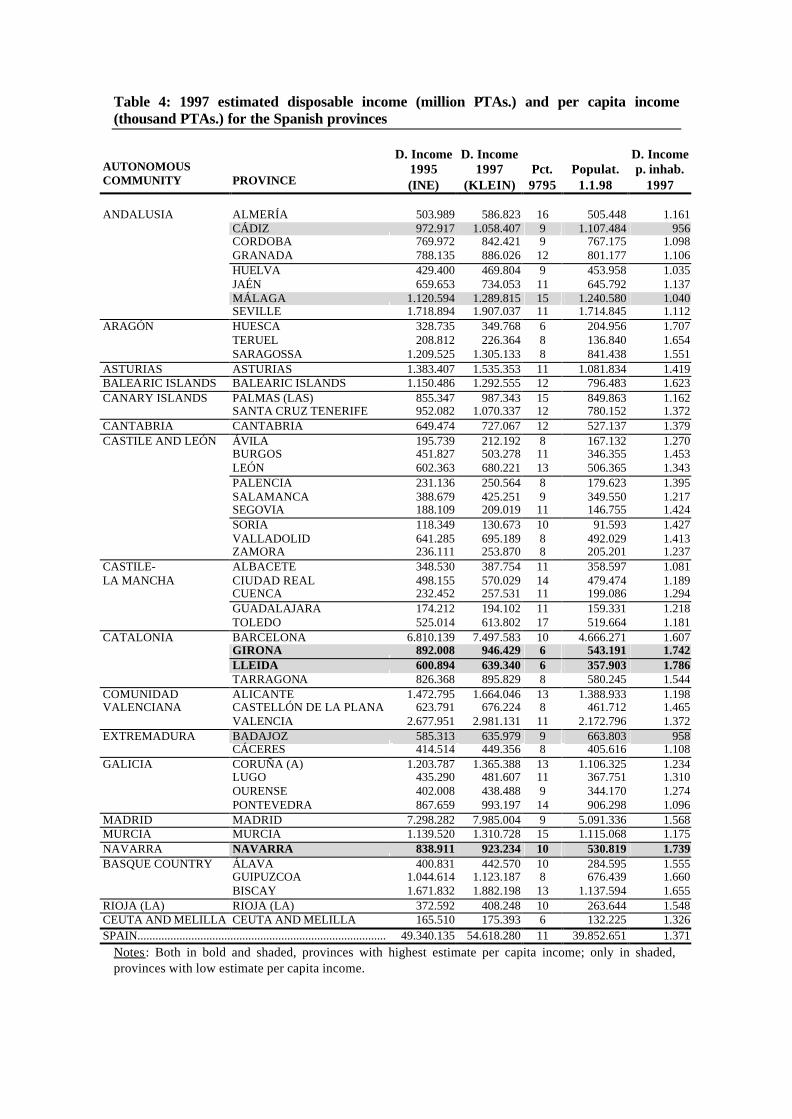
Table 4: 1997 estimated disposable income (million PTAs.) and per capita income (thousand PTAs.) for the Spanish provinces

AUTONOMOUS COMMUNITY

PROVINCE

D. Income 1995 (INE)

D. Income 1997

(KLEIN)

Pct. 9795

Populat.

1.1.98

D. Income p. inhab.

1997 ANDALUSIA

ALMERÍA

503.989

586.823

16

505.448

1.161

CÁDIZ 972.917 1.058.407 9 1.107.484 956 CORDOBA 769.972 842.421 9 767.175 1.098 GRANADA 788.135 886.026 12 801.177 1.106 HUELVA 429.400 469.804 9 453.958 1.035 JAÉN 659.653 734.053 11 645.792 1.137 MÁLAGA 1.120.594 1.289.815 15 1.240.580 1.040 SEVILLE 1.718.894 1.907.037 11 1.714.845 1.112 ARAGÓN HUESCA 328.735 349.768 6 204.956 1.707 TERUEL 208.812 226.364 8 136.840 1.654 SARAGOSSA 1.209.525 1.305.133 8 841.438 1.551 ASTURIAS ASTURIAS 1.383.407 1.535.353 11 1.081.834 1.419 BALEARIC ISLANDS BALEARIC ISLANDS 1.150.486 1.292.555 12 796.483 1.623 CANARY ISLANDS PALMAS (LAS) 855.347 987.343 15 849.863 1.162 SANTA CRUZ TENERIFE 952.082 1.070.337 12 780.152 1.372 CANTABRIA CANTABRIA 649.474 727.067 12 527.137 1.379 CASTILE AND LEÓN ÁVILA 195.739 212.192 8 167.132 1.270 BURGOS 451.827 503.278 11 346.355 1.453 LEÓN 602.363 680.221 13 506.365 1.343 PALENCIA 231.136 250.564 8 179.623 1.395 SALAMANCA 388.679 425.251 9 349.550 1.217 SEGOVIA 188.109 209.019 11 146.755 1.424 SORIA 118.349 130.673 10 91.593 1.427 VALLADOLID 641.285 695.189 8 492.029 1.413 ZAMORA 236.111 253.870 8 205.201 1.237 CASTILE- ALBACETE 348.530 387.754 11 358.597 1.081 LA MANCHA CIUDAD REAL 498.155 570.029 14 479.474 1.189 CUENCA 232.452 257.531 11 199.086 1.294 GUADALAJARA 174.212 194.102 11 159.331 1.218 TOLEDO 525.014 613.802 17 519.664 1.181 CATALONIA BARCELONA 6.810.139 7.497.583 10 4.666.271 1.607 GIRONA 892.008 946.429 6 543.191 1.742 LLEIDA 600.894 639.340 6 357.903 1.786 TARRAGONA 826.368 895.829 8 580.245 1.544 COMUNIDAD ALICANTE 1.472.795 1.664.046 13 1.388.933 1.198 VALENCIANA CASTELLÓN DE LA PLANA 623.791 676.224 8 461.712 1.465 VALENCIA 2.677.951 2.981.131 11 2.172.796 1.372 EXTREMADURA BADAJOZ 585.313 635.979 9 663.803 958 CÁCERES 414.514 449.356 8 405.616 1.108 GALICIA CORUÑA (A) 1.203.787 1.365.388 13 1.106.325 1.234 LUGO 435.290 481.607 11 367.751 1.310 OURENSE 402.008 438.488 9 344.170 1.274 PONTEVEDRA 867.659 993.197 14 906.298 1.096 MADRID MADRID 7.298.282 7.985.004 9 5.091.336 1.568 MURCIA MURCIA 1.139.520 1.310.728 15 1.115.068 1.175 NAVARRA NAVARRA 838.911 923.234 10 530.819 1.739 BASQUE COUNTRY ÁLAVA 400.831 442.570 10 284.595 1.555 GUIPUZCOA 1.044.614 1.123.187 8 676.439 1.660 BISCAY 1.671.832 1.882.198 13 1.137.594 1.655 RIOJA (LA) RIOJA (LA) 372.592 408.248 10 263.644 1.548 CEUTA AND MELILLA CEUTA AND MELILLA 165.510 175.393 6 132.225 1.326 SPAIN................................................................................... 49.340.135 54.618.280 11 39.852.651 1.371

Notes: Both in bold and shaded, provinces with highest estimate per capita income; only in shaded, provinces with low estimate per capita income.

4. ESTIMATION OF THE 1997 MUNICIPAL DISPOSABLE INCOME Once estimated the 1997 provincial disposable income, they will constitute the endogenous variables of a final multiple-regression model with new explicative variables available –in this case- for the municipal level. 4.1. Selection of new explicative variables related with disposable personal income,

also available for the municipal level In this step, a new selection of explicate variables must be carried out as they have also to be available for the municipal level –in Spain there are actually 8.099 municipalities. This kind of micro-data is still difficult to obtain in Spain as official Census data are mainly outdated and only referred to demographic items. That is why Klein Institute has tackled the problem of developing a big updated municipal socio-economic database. In the starting point, there were 66 municipal variables in any way correlated with disposable income, that have been reduced to 20 selected explicative variables (Table 4). These indicators –all rated by population- will be determinant in the municipal estimation because of their big correlation with disposable income. Table 4: Explicative variables available for the municipal level and per capita Cars Building industry establishments Banks Restaurants, bars and cafeterias Savings banks Industry establishments Credit co-operatives Wholesale establishments Vans and lorries Unemployment rate –16-24 year old. Average distance to retailing trade areas Unemployment rate –building industry sector 1992-97 Pct. cars Unemployment rate –industry sector 1991-96 Pct. population Unemployment rate –public sector 1992-97 Pct. domestic telephone lines Unemployment rate –private sector Tourism establishments rooms Domestic telephone lines Notice than in this occasion we have considered domestic telephone lines instead of the total ones –domestic and business ones. Telephone lines variable is still determinant because of its great correlation with disposable income; nevertheless, its influence over provincial income data is not in the same as over municipal ones. In the municipal level, domestic lines are determinant in a 100%, while business ones must only be considered in a 25% -as we have measured business activity influence over disposable income in a quarter of the total. Therefore, the so-called ‘domestic telephone lines’ variable includes no only the 100% of domestic but also business lines in a 25%. This correction helps to avoid certain biased values due to income overestimation in certain little or middle-sized income generating municipalities –because of industry or tourism activity- produced by the total telephone lines variable. This problem can be corrected by the consideration of only the domestic and the 25% of business lines.

4.2. Factor analysis of 20 income explicative variables for the provincial level As it has been showed, in order to include as much information as possible in the final model avoiding multicolinearity, it is advisable to carry out a factor analysis of the 20 selected indicators. In this occasion, we consider a 50x20 matrix data in order to construct unique factors as exogenous variables in the spatial multiple-regression model. The analysis produces 4 factors with 77% of cumulative variance. In Table 5, we present a summary of these factors obtained with Varimax rotation. Table 5: Factor structure of variables related with provincial disposable income also available for the municipal level FAC. 1: SERVICE SECTOR ACTIVITY Provinces with big concentration of all kind of service sector activity, high occupation rates and good infrastructure equipment.

FAC. 2: SECONDARY SECTOR & EMPLOYMENT Provinces with big concentration of secondary sector activity –industry and building- and low unemployment rates.

FAC. 3: POPULATION GROWING & TOURISM Provinces with high rates of immigration during the last 5 years, high number of cars, vans, lorries and predominant tourism and trade activity.

FAC. 4: UNDERDEVELOPEMENT Provinces with traditional economic and infrastructure underdevelopment, high unemployment rates, but quick recent growth in their standards of living.

FAC. 5: INDUSTRIAL DEVELOPMENT Provinces with industrial development but high rates of unemployment. 4.3. Cross-section multiple regression for the 1997 provincial disposable income These 5 factors will be the explicate variables in a multiple regression analysis with estimated provincial disposable income for 1997. The final model (Eq. 8, Table 6) excludes factor 3 –Population growing & tourism- as it was not significant, but includes 3 dummy variables –FORAL, LAST, FIRST- which take account spatial heterogeneity in disposable income distribution (Fig. 2).

iULAST7FIRST6FORAL5F54F43F22F110iDI +β+β+β+β+β+β+β+β=

Eq. 8

with: DIi: 1997 per capita provincial disposable income, i = 1...50. F1...F5: factors, F1 –Service sector activity, F2 –Secondary sector &

employment, F4 –Underdevelopment, F5 –Industrial development. FORAL: Basque Country provinces, with underestimate income.

FIRST: Provinces with significantly higher income than their neighbours – Huesca, Lleida, Madrid, Santa Cruz de Tenerife, Teruel, and Saragossa.

LAST: Provinces with significantly lower income than their neighbours –Alicante, Cáceres, Guadalajara, Murcia, Pontevedra and Toledo.

Figure 2: Spatial distribution of 1997 provincial disposable income per inhabitant

Notes: It is represented the provinces with value 1 en dummy variables –FORAL, L (LAST), F (FIRST). Disposable income distribution over the Spanish provinces produces some geographical irregularities –spatial heterogeneity- not always correctly reflected by the model. Dummy variables takes account these phenomenon. Table 6: Multiple regression results Dependent Variable: DI Method: Least Squares Sample: 1 50 Included observations: 50

Variable Coefficient Std. Error t-Statistic Prob.

C 1.076628 0.009574 112.4566 0.0000F1 0.105510 0.007584 13.91273 0.0000F2 0.062022 0.007817 7.934271 0.0000F4 -0.059475 0.007956 -7.475217 0.0000F5 0.028242 0.007934 3.559518 0.0009

FORAL 0.166096 0.030392 5.465122 0.0000LAST -0.105701 0.021508 -4.914590 0.0000FIRST 0.187301 0.024625 7.606142 0.0000

R-squared 0.928269 Mean dependent var 1.095480Adjusted R-squared 0.916313 S.D. dependent var 0.182062S.E. of regression 0.052668 Akaike info criterion -2.903967Sum squared resid 0.116505 Schwarz criterion -2.598043Log likelihood 80.59917 F-statistic 77.64537Durbin-Watson stat

1.300678 Prob(F-statistic) 0.000000

L

L

L

L

L

F

L

F

F

F

FORAL

F

F

4.4. Estimation of 1997 municipal disposable income As the previous statistical tests are correct, now it is possible to obtain the municipal income data. First, as explicate variables were also available to municipal level it is necessary to estimate factor municipal values using the factor scores to apply over them the estimate regression parameters. The resulting municipal data must be adjusted by 2 corrective coefficient:

1. Ratio of business tax –IAE in Spain- corresponding to liberal professionals over total business tax which detects those high- level localities without a special generating economic activity. Indirect income estimations tend to underestimate disposable income in these towns because of the relatively low values of explicative indicators related with economic activity.

2. The resulting municipal data must be adjusted so that the sum of municipal income values coincides with provincial ones.

In Figure 3, we present the municipal estimations of disposable income. As it can be seen, in Spain per capita disposable income distributes progressively from the south to the northeast, being Extremadura and Andalusia the poorest regions followed by Castille-La Mancha, Murcia and Galicia. In the other side, the highest levels of disposable income can be found in Navarra, the Balearic Islands, the Basque Country, Catalonia and Madrid. Figure 3: 1997 estimated per capita disposable income for the 8.099 Spanish municipalities Spanish South Spanish Northwest

CACERESCACERESCACERESCACERESCACERESCACERESCACERESCACERESCACERESCACERESCACERESCACERESCACERESCACERESCACERESCACERESCACERESCACERESCACERESCACERESCACERESCACERESCACERESCACERESCACERESCACERESCACERESCACERESCACERESCACERESCACERESCACERESCACERESCACERESCACERESCACERESCACERESCACERESCACERESCACERESCACERESCACERESCACERESCACERESCACERESCACERESCACERESCACERESCACERES

VIZCAYAVIZCAYAVIZCAYAVIZCAYAVIZCAYAVIZCAYAVIZCAYAVIZCAYAVIZCAYAVIZCAYAVIZCAYAVIZCAYAVIZCAYAVIZCAYAVIZCAYAVIZCAYAVIZCAYAVIZCAYAVIZCAYAVIZCAYAVIZCAYAVIZCAYAVIZCAYAVIZCAYAVIZCAYAVIZCAYAVIZCAYAVIZCAYAVIZCAYAVIZCAYAVIZCAYAVIZCAYAVIZCAYAVIZCAYAVIZCAYAVIZCAYAVIZCAYAVIZCAYAVIZCAYAVIZCAYAVIZCAYAVIZCAYAVIZCAYAVIZCAYAVIZCAYAVIZCAYAVIZCAYAVIZCAYAVIZCAYA

CANTABRIACANTABRIACANTABRIACANTABRIACANTABRIACANTABRIACANTABRIACANTABRIACANTABRIACANTABRIACANTABRIACANTABRIACANTABRIACANTABRIACANTABRIACANTABRIACANTABRIACANTABRIACANTABRIACANTABRIACANTABRIACANTABRIACANTABRIACANTABRIACANTABRIACANTABRIACANTABRIACANTABRIACANTABRIACANTABRIACANTABRIACANTABRIACANTABRIACANTABRIACANTABRIACANTABRIACANTABRIACANTABRIACANTABRIACANTABRIACANTABRIACANTABRIACANTABRIACANTABRIACANTABRIACANTABRIACANTABRIACANTABRIACANTABRIAA CORUÑAA CORUÑAA CORUÑAA CORUÑAA CORUÑAA CORUÑAA CORUÑAA CORUÑAA CORUÑAA CORUÑAA CORUÑAA CORUÑAA CORUÑAA CORUÑAA CORUÑAA CORUÑAA CORUÑAA CORUÑAA CORUÑAA CORUÑAA CORUÑAA CORUÑAA CORUÑAA CORUÑAA CORUÑAA CORUÑAA CORUÑAA CORUÑAA CORUÑAA CORUÑAA CORUÑAA CORUÑAA CORUÑAA CORUÑAA CORUÑAA CORUÑAA CORUÑAA CORUÑAA CORUÑAA CORUÑAA CORUÑAA CORUÑAA CORUÑAA CORUÑAA CORUÑAA CORUÑAA CORUÑAA CORUÑAA CORUÑA

SEGOVIASEGOVIASEGOVIASEGOVIASEGOVIASEGOVIASEGOVIASEGOVIASEGOVIASEGOVIASEGOVIASEGOVIASEGOVIASEGOVIASEGOVIASEGOVIASEGOVIASEGOVIASEGOVIASEGOVIASEGOVIASEGOVIASEGOVIASEGOVIASEGOVIASEGOVIASEGOVIASEGOVIASEGOVIASEGOVIASEGOVIASEGOVIASEGOVIASEGOVIASEGOVIASEGOVIASEGOVIASEGOVIASEGOVIASEGOVIASEGOVIASEGOVIASEGOVIASEGOVIASEGOVIASEGOVIASEGOVIASEGOVIASEGOVIA

VALLADOLIDVALLADOLIDVALLADOLIDVALLADOLIDVALLADOLIDVALLADOLIDVALLADOLIDVALLADOLIDVALLADOLIDVALLADOLIDVALLADOLIDVALLADOLIDVALLADOLIDVALLADOLIDVALLADOLIDVALLADOLIDVALLADOLIDVALLADOLIDVALLADOLIDVALLADOLIDVALLADOLIDVALLADOLIDVALLADOLIDVALLADOLIDVALLADOLIDVALLADOLIDVALLADOLIDVALLADOLIDVALLADOLIDVALLADOLIDVALLADOLIDVALLADOLIDVALLADOLIDVALLADOLIDVALLADOLIDVALLADOLIDVALLADOLIDVALLADOLIDVALLADOLIDVALLADOLIDVALLADOLIDVALLADOLIDVALLADOLIDVALLADOLIDVALLADOLIDVALLADOLIDVALLADOLIDVALLADOLIDVALLADOLID

MADRIDMADRIDMADRIDMADRIDMADRIDMADRIDMADRIDMADRIDMADRIDMADRIDMADRIDMADRIDMADRIDMADRIDMADRIDMADRIDMADRIDMADRIDMADRIDMADRIDMADRIDMADRIDMADRIDMADRIDMADRIDMADRIDMADRIDMADRIDMADRIDMADRIDMADRIDMADRIDMADRIDMADRIDMADRIDMADRIDMADRIDMADRIDMADRIDMADRIDMADRIDMADRIDMADRIDMADRIDMADRIDMADRIDMADRIDMADRIDMADRID

SALAMANCASALAMANCASALAMANCASALAMANCASALAMANCASALAMANCASALAMANCASALAMANCASALAMANCASALAMANCASALAMANCASALAMANCASALAMANCASALAMANCASALAMANCASALAMANCASALAMANCASALAMANCASALAMANCASALAMANCASALAMANCASALAMANCASALAMANCASALAMANCASALAMANCASALAMANCASALAMANCASALAMANCASALAMANCASALAMANCASALAMANCASALAMANCASALAMANCASALAMANCASALAMANCASALAMANCASALAMANCASALAMANCASALAMANCASALAMANCASALAMANCASALAMANCASALAMANCASALAMANCASALAMANCASALAMANCASALAMANCASALAMANCASALAMANCA

ZAMORAZAMORAZAMORAZAMORAZAMORAZAMORAZAMORAZAMORAZAMORAZAMORAZAMORAZAMORAZAMORAZAMORAZAMORAZAMORAZAMORAZAMORAZAMORAZAMORAZAMORAZAMORAZAMORAZAMORAZAMORAZAMORAZAMORAZAMORAZAMORAZAMORAZAMORAZAMORAZAMORAZAMORAZAMORAZAMORAZAMORAZAMORAZAMORAZAMORAZAMORAZAMORAZAMORAZAMORAZAMORAZAMORAZAMORAZAMORAZAMORAORENSEORENSEORENSEORENSEORENSEORENSEORENSEORENSEORENSEORENSEORENSEORENSEORENSEORENSEORENSEORENSEORENSEORENSEORENSEORENSEORENSEORENSEORENSEORENSEORENSEORENSEORENSEORENSEORENSEORENSEORENSEORENSEORENSEORENSEORENSEORENSEORENSEORENSEORENSEORENSEORENSEORENSEORENSEORENSEORENSEORENSEORENSEORENSEORENSE

PONTEVEDRAPONTEVEDRAPONTEVEDRAPONTEVEDRAPONTEVEDRAPONTEVEDRAPONTEVEDRAPONTEVEDRAPONTEVEDRAPONTEVEDRAPONTEVEDRAPONTEVEDRAPONTEVEDRAPONTEVEDRAPONTEVEDRAPONTEVEDRAPONTEVEDRAPONTEVEDRAPONTEVEDRAPONTEVEDRAPONTEVEDRAPONTEVEDRAPONTEVEDRAPONTEVEDRAPONTEVEDRAPONTEVEDRAPONTEVEDRAPONTEVEDRAPONTEVEDRAPONTEVEDRAPONTEVEDRAPONTEVEDRAPONTEVEDRAPONTEVEDRAPONTEVEDRAPONTEVEDRAPONTEVEDRAPONTEVEDRAPONTEVEDRAPONTEVEDRAPONTEVEDRAPONTEVEDRAPONTEVEDRAPONTEVEDRAPONTEVEDRAPONTEVEDRAPONTEVEDRAPONTEVEDRAPONTEVEDRA

LUGOLUGOLUGOLUGOLUGOLUGOLUGOLUGOLUGOLUGOLUGOLUGOLUGOLUGOLUGOLUGOLUGOLUGOLUGOLUGOLUGOLUGOLUGOLUGOLUGOLUGOLUGOLUGOLUGOLUGOLUGOLUGOLUGOLUGOLUGOLUGOLUGOLUGOLUGOLUGOLUGOLUGOLUGOLUGOLUGOLUGOLUGOLUGOLUGOALAVAALAVAALAVAALAVAALAVAALAVAALAVAALAVAALAVAALAVAALAVAALAVAALAVAALAVAALAVAALAVAALAVAALAVAALAVAALAVAALAVAALAVAALAVAALAVAALAVAALAVAALAVAALAVAALAVAALAVAALAVAALAVAALAVAALAVAALAVAALAVAALAVAALAVAALAVAALAVAALAVAALAVAALAVAALAVAALAVAALAVAALAVAALAVAALAVA

AVILAAVILAAVILAAVILAAVILAAVILAAVILAAVILAAVILAAVILAAVILAAVILAAVILAAVILAAVILAAVILAAVILAAVILAAVILAAVILAAVILAAVILAAVILAAVILAAVILAAVILAAVILAAVILAAVILAAVILAAVILAAVILAAVILAAVILAAVILAAVILAAVILAAVILAAVILAAVILAAVILAAVILAAVILAAVILAAVILAAVILAAVILAAVILAAVILA

BURGOSBURGOSBURGOSBURGOSBURGOSBURGOSBURGOSBURGOSBURGOSBURGOSBURGOSBURGOSBURGOSBURGOSBURGOSBURGOSBURGOSBURGOSBURGOSBURGOSBURGOSBURGOSBURGOSBURGOSBURGOSBURGOSBURGOSBURGOSBURGOSBURGOSBURGOSBURGOSBURGOSBURGOSBURGOSBURGOSBURGOSBURGOSBURGOSBURGOSBURGOSBURGOSBURGOSBURGOSBURGOSBURGOSBURGOSBURGOSBURGOS

CUENCACUENCACUENCACUENCACUENCACUENCACUENCACUENCACUENCACUENCACUENCACUENCACUENCACUENCACUENCACUENCACUENCACUENCACUENCACUENCACUENCACUENCACUENCACUENCACUENCACUENCACUENCACUENCACUENCACUENCACUENCACUENCACUENCACUENCACUENCACUENCACUENCACUENCACUENCACUENCACUENCACUENCACUENCACUENCACUENCACUENCACUENCACUENCACUENCA

GUADALAJARGUADALAJARGUADALAJARGUADALAJARGUADALAJARGUADALAJARGUADALAJARGUADALAJARGUADALAJARGUADALAJARGUADALAJARGUADALAJARGUADALAJARGUADALAJARGUADALAJARGUADALAJARGUADALAJARGUADALAJARGUADALAJARGUADALAJARGUADALAJARGUADALAJARGUADALAJARGUADALAJARGUADALAJARGUADALAJARGUADALAJARGUADALAJARGUADALAJARGUADALAJARGUADALAJARGUADALAJARGUADALAJARGUADALAJARGUADALAJARGUADALAJARGUADALAJARGUADALAJARGUADALAJARGUADALAJARGUADALAJARGUADALAJARGUADALAJARGUADALAJARGUADALAJARGUADALAJARGUADALAJARGUADALAJARGUADALAJAR

LEONLEONLEONLEONLEONLEONLEONLEONLEONLEONLEONLEONLEONLEONLEONLEONLEONLEONLEONLEONLEONLEONLEONLEONLEONLEONLEONLEONLEONLEONLEONLEONLEONLEONLEONLEONLEONLEONLEONLEONLEONLEONLEONLEONLEONLEONLEONLEONLEON

ASTURIASASTURIASASTURIASASTURIASASTURIASASTURIASASTURIASASTURIASASTURIASASTURIASASTURIASASTURIASASTURIASASTURIASASTURIASASTURIASASTURIASASTURIASASTURIASASTURIASASTURIASASTURIASASTURIASASTURIASASTURIASASTURIASASTURIASASTURIASASTURIASASTURIASASTURIASASTURIASASTURIASASTURIASASTURIASASTURIASASTURIASASTURIASASTURIASASTURIASASTURIASASTURIASASTURIASASTURIASASTURIASASTURIASASTURIASASTURIASASTURIAS

SORIASORIASORIASORIASORIASORIASORIASORIASORIASORIASORIASORIASORIASORIASORIASORIASORIASORIASORIASORIASORIASORIASORIASORIASORIASORIASORIASORIASORIASORIASORIASORIASORIASORIASORIASORIASORIASORIASORIASORIASORIASORIASORIASORIASORIASORIASORIASORIASORIA

TOLEDOTOLEDOTOLEDOTOLEDOTOLEDOTOLEDOTOLEDOTOLEDOTOLEDOTOLEDOTOLEDOTOLEDOTOLEDOTOLEDOTOLEDOTOLEDOTOLEDOTOLEDOTOLEDOTOLEDOTOLEDOTOLEDOTOLEDOTOLEDOTOLEDOTOLEDOTOLEDOTOLEDOTOLEDOTOLEDOTOLEDOTOLEDOTOLEDOTOLEDOTOLEDOTOLEDOTOLEDOTOLEDOTOLEDOTOLEDOTOLEDOTOLEDOTOLEDOTOLEDOTOLEDOTOLEDOTOLEDOTOLEDOTOLEDOCeuta

Melilla

CACERESCACERESCACERESCACERESCACERESCACERESCACERESCACERESCACERESCACERESCACERESCACERESCACERESCACERESCACERESCACERESCACERESCACERESCACERESCACERESCACERESCACERESCACERESCACERESCACERESCACERESCACERESCACERESCACERESCACERESCACERESCACERESCACERESCACERESCACERESCACERESCACERESCACERESCACERESCACERESCACERESCACERESCACERESCACERESCACERESCACERESCACERESCACERESCACERES

BADAJOZBADAJOZBADAJOZBADAJOZBADAJOZBADAJOZBADAJOZBADAJOZBADAJOZBADAJOZBADAJOZBADAJOZBADAJOZBADAJOZBADAJOZBADAJOZBADAJOZBADAJOZBADAJOZBADAJOZBADAJOZBADAJOZBADAJOZBADAJOZBADAJOZBADAJOZBADAJOZBADAJOZBADAJOZBADAJOZBADAJOZBADAJOZBADAJOZBADAJOZBADAJOZBADAJOZBADAJOZBADAJOZBADAJOZBADAJOZBADAJOZBADAJOZBADAJOZBADAJOZBADAJOZBADAJOZBADAJOZBADAJOZBADAJOZ

CIUDAD REALCIUDAD REALCIUDAD REALCIUDAD REALCIUDAD REALCIUDAD REALCIUDAD REALCIUDAD REALCIUDAD REALCIUDAD REALCIUDAD REALCIUDAD REALCIUDAD REALCIUDAD REALCIUDAD REALCIUDAD REALCIUDAD REALCIUDAD REALCIUDAD REALCIUDAD REALCIUDAD REALCIUDAD REALCIUDAD REALCIUDAD REALCIUDAD REALCIUDAD REALCIUDAD REALCIUDAD REALCIUDAD REALCIUDAD REALCIUDAD REALCIUDAD REALCIUDAD REALCIUDAD REALCIUDAD REALCIUDAD REALCIUDAD REALCIUDAD REALCIUDAD REALCIUDAD REALCIUDAD REALCIUDAD REALCIUDAD REALCIUDAD REALCIUDAD REALCIUDAD REALCIUDAD REALCIUDAD REALCIUDAD REALALBACETEALBACETEALBACETEALBACETEALBACETEALBACETEALBACETEALBACETEALBACETEALBACETEALBACETEALBACETEALBACETEALBACETEALBACETEALBACETEALBACETEALBACETEALBACETEALBACETEALBACETEALBACETEALBACETEALBACETEALBACETEALBACETEALBACETEALBACETEALBACETEALBACETEALBACETEALBACETEALBACETEALBACETEALBACETEALBACETEALBACETEALBACETEALBACETEALBACETEALBACETEALBACETEALBACETEALBACETEALBACETEALBACETEALBACETEALBACETEALBACETE

GRANADAGRANADAGRANADAGRANADAGRANADAGRANADAGRANADAGRANADAGRANADAGRANADAGRANADAGRANADAGRANADAGRANADAGRANADAGRANADAGRANADAGRANADAGRANADAGRANADAGRANADAGRANADAGRANADAGRANADAGRANADAGRANADAGRANADAGRANADAGRANADAGRANADAGRANADAGRANADAGRANADAGRANADAGRANADAGRANADAGRANADAGRANADAGRANADAGRANADAGRANADAGRANADAGRANADAGRANADAGRANADAGRANADAGRANADAGRANADAGRANADA ALMERIAALMERIAALMERIAALMERIAALMERIAALMERIAALMERIAALMERIAALMERIAALMERIAALMERIAALMERIAALMERIAALMERIAALMERIAALMERIAALMERIAALMERIAALMERIAALMERIAALMERIAALMERIAALMERIAALMERIAALMERIAALMERIAALMERIAALMERIAALMERIAALMERIAALMERIAALMERIAALMERIAALMERIAALMERIAALMERIAALMERIAALMERIAALMERIAALMERIAALMERIAALMERIAALMERIAALMERIAALMERIAALMERIAALMERIAALMERIAALMERIA

CADIZCADIZCADIZCADIZCADIZCADIZCADIZCADIZCADIZCADIZCADIZCADIZCADIZCADIZCADIZCADIZCADIZCADIZCADIZCADIZCADIZCADIZCADIZCADIZCADIZCADIZCADIZCADIZCADIZCADIZCADIZCADIZCADIZCADIZCADIZCADIZCADIZCADIZCADIZCADIZCADIZCADIZCADIZCADIZCADIZCADIZCADIZCADIZCADIZ

CORDOBACORDOBACORDOBACORDOBACORDOBACORDOBACORDOBACORDOBACORDOBACORDOBACORDOBACORDOBACORDOBACORDOBACORDOBACORDOBACORDOBACORDOBACORDOBACORDOBACORDOBACORDOBACORDOBACORDOBACORDOBACORDOBACORDOBACORDOBACORDOBACORDOBACORDOBACORDOBACORDOBACORDOBACORDOBACORDOBACORDOBACORDOBACORDOBACORDOBACORDOBACORDOBACORDOBACORDOBACORDOBACORDOBACORDOBACORDOBACORDOBA

HUELVAHUELVAHUELVAHUELVAHUELVAHUELVAHUELVAHUELVAHUELVAHUELVAHUELVAHUELVAHUELVAHUELVAHUELVAHUELVAHUELVAHUELVAHUELVAHUELVAHUELVAHUELVAHUELVAHUELVAHUELVAHUELVAHUELVAHUELVAHUELVAHUELVAHUELVAHUELVAHUELVAHUELVAHUELVAHUELVAHUELVAHUELVAHUELVAHUELVAHUELVAHUELVAHUELVAHUELVAHUELVAHUELVAHUELVAHUELVAHUELVA

JAENJAENJAENJAENJAENJAENJAENJAENJAENJAENJAENJAENJAENJAENJAENJAENJAENJAENJAENJAENJAENJAENJAENJAENJAENJAENJAENJAENJAENJAENJAENJAENJAENJAENJAENJAENJAENJAENJAENJAENJAENJAENJAENJAENJAENJAENJAENJAENJAEN

MALAGAMALAGAMALAGAMALAGAMALAGAMALAGAMALAGAMALAGAMALAGAMALAGAMALAGAMALAGAMALAGAMALAGAMALAGAMALAGAMALAGAMALAGAMALAGAMALAGAMALAGAMALAGAMALAGAMALAGAMALAGAMALAGAMALAGAMALAGAMALAGAMALAGAMALAGAMALAGAMALAGAMALAGAMALAGAMALAGAMALAGAMALAGAMALAGAMALAGAMALAGAMALAGAMALAGAMALAGAMALAGAMALAGAMALAGAMALAGAMALAGA

MURCIAMURCIAMURCIAMURCIAMURCIAMURCIAMURCIAMURCIAMURCIAMURCIAMURCIAMURCIAMURCIAMURCIAMURCIAMURCIAMURCIAMURCIAMURCIAMURCIAMURCIAMURCIAMURCIAMURCIAMURCIAMURCIAMURCIAMURCIAMURCIAMURCIAMURCIAMURCIAMURCIAMURCIAMURCIAMURCIAMURCIAMURCIAMURCIAMURCIAMURCIAMURCIAMURCIAMURCIAMURCIAMURCIAMURCIAMURCIAMURCIA

SEVILLASEVILLASEVILLASEVILLASEVILLASEVILLASEVILLASEVILLASEVILLASEVILLASEVILLASEVILLASEVILLASEVILLASEVILLASEVILLASEVILLASEVILLASEVILLASEVILLASEVILLASEVILLASEVILLASEVILLASEVILLASEVILLASEVILLASEVILLASEVILLASEVILLASEVILLASEVILLASEVILLASEVILLASEVILLASEVILLASEVILLASEVILLASEVILLASEVILLASEVILLASEVILLASEVILLASEVILLASEVILLASEVILLASEVILLASEVILLASEVILLA

TOLEDOTOLEDOTOLEDOTOLEDOTOLEDOTOLEDOTOLEDOTOLEDOTOLEDOTOLEDOTOLEDOTOLEDOTOLEDOTOLEDOTOLEDOTOLEDOTOLEDOTOLEDOTOLEDOTOLEDOTOLEDOTOLEDOTOLEDOTOLEDOTOLEDOTOLEDOTOLEDOTOLEDOTOLEDOTOLEDOTOLEDOTOLEDOTOLEDOTOLEDOTOLEDOTOLEDOTOLEDOTOLEDOTOLEDOTOLEDOTOLEDOTOLEDOTOLEDOTOLEDOTOLEDOTOLEDOTOLEDOTOLEDOTOLEDO

VALENCIAVALENCIAVALENCIAVALENCIAVALENCIAVALENCIAVALENCIAVALENCIAVALENCIAVALENCIAVALENCIAVALENCIAVALENCIAVALENCIAVALENCIAVALENCIAVALENCIAVALENCIAVALENCIAVALENCIAVALENCIAVALENCIAVALENCIAVALENCIAVALENCIAVALENCIAVALENCIAVALENCIAVALENCIAVALENCIAVALENCIAVALENCIAVALENCIAVALENCIAVALENCIAVALENCIAVALENCIAVALENCIAVALENCIAVALENCIAVALENCIAVALENCIAVALENCIAVALENCIAVALENCIAVALENCIAVALENCIAVALENCIAVALENCIA

Spanish Northeast The Canary Islands

Notes: In red, more than 1.600.000 PTA./inhab. In red, 1.125.000-1.600.000 PTA./inhab. In yellow, less than 1.125.000 PTA./inhab.

LAS PALMASSANTA CRUZDE TENERIFE

GUADALAJARAGUADALAJARAGUADALAJARAGUADALAJARAGUADALAJARAGUADALAJARAGUADALAJARAGUADALAJARAGUADALAJARAGUADALAJARAGUADALAJARAGUADALAJARAGUADALAJARAGUADALAJARAGUADALAJARAGUADALAJARAGUADALAJARAGUADALAJARAGUADALAJARAGUADALAJARAGUADALAJARAGUADALAJARAGUADALAJARAGUADALAJARAGUADALAJARAGUADALAJARAGUADALAJARAGUADALAJARAGUADALAJARAGUADALAJARAGUADALAJARAGUADALAJARAGUADALAJARAGUADALAJARAGUADALAJARAGUADALAJARAGUADALAJARAGUADALAJARAGUADALAJARAGUADALAJARAGUADALAJARAGUADALAJARAGUADALAJARAGUADALAJARAGUADALAJARAGUADALAJARAGUADALAJARAGUADALAJARAGUADALAJARATERUELTERUELTERUELTERUELTERUELTERUELTERUELTERUELTERUELTERUELTERUELTERUELTERUELTERUELTERUELTERUELTERUELTERUELTERUELTERUELTERUELTERUELTERUELTERUELTERUELTERUELTERUELTERUELTERUELTERUELTERUELTERUELTERUELTERUELTERUELTERUELTERUELTERUELTERUELTERUELTERUELTERUELTERUELTERUELTERUELTERUELTERUELTERUELTERUEL

VIZCAYAVIZCAYAVIZCAYAVIZCAYAVIZCAYAVIZCAYAVIZCAYAVIZCAYAVIZCAYAVIZCAYAVIZCAYAVIZCAYAVIZCAYAVIZCAYAVIZCAYAVIZCAYAVIZCAYAVIZCAYAVIZCAYAVIZCAYAVIZCAYAVIZCAYAVIZCAYAVIZCAYAVIZCAYAVIZCAYAVIZCAYAVIZCAYAVIZCAYAVIZCAYAVIZCAYAVIZCAYAVIZCAYAVIZCAYAVIZCAYAVIZCAYAVIZCAYAVIZCAYAVIZCAYAVIZCAYAVIZCAYAVIZCAYAVIZCAYAVIZCAYAVIZCAYAVIZCAYAVIZCAYAVIZCAYAVIZCAYA GUIPUZCOAGUIPUZCOAGUIPUZCOAGUIPUZCOAGUIPUZCOAGUIPUZCOAGUIPUZCOAGUIPUZCOAGUIPUZCOAGUIPUZCOAGUIPUZCOAGUIPUZCOAGUIPUZCOAGUIPUZCOAGUIPUZCOAGUIPUZCOAGUIPUZCOAGUIPUZCOAGUIPUZCOAGUIPUZCOAGUIPUZCOAGUIPUZCOAGUIPUZCOAGUIPUZCOAGUIPUZCOAGUIPUZCOAGUIPUZCOAGUIPUZCOAGUIPUZCOAGUIPUZCOAGUIPUZCOAGUIPUZCOAGUIPUZCOAGUIPUZCOAGUIPUZCOAGUIPUZCOAGUIPUZCOAGUIPUZCOAGUIPUZCOAGUIPUZCOAGUIPUZCOAGUIPUZCOAGUIPUZCOAGUIPUZCOAGUIPUZCOAGUIPUZCOAGUIPUZCOAGUIPUZCOAGUIPUZCOA

ALBACETEALBACETEALBACETEALBACETEALBACETEALBACETEALBACETEALBACETEALBACETEALBACETEALBACETEALBACETEALBACETEALBACETEALBACETEALBACETEALBACETEALBACETEALBACETEALBACETEALBACETEALBACETEALBACETEALBACETEALBACETEALBACETEALBACETEALBACETEALBACETEALBACETEALBACETEALBACETEALBACETEALBACETEALBACETEALBACETEALBACETEALBACETEALBACETEALBACETEALBACETEALBACETEALBACETEALBACETEALBACETEALBACETEALBACETEALBACETEALBACETE

NAVARRANAVARRANAVARRANAVARRANAVARRANAVARRANAVARRANAVARRANAVARRANAVARRANAVARRANAVARRANAVARRANAVARRANAVARRANAVARRANAVARRANAVARRANAVARRANAVARRANAVARRANAVARRANAVARRANAVARRANAVARRANAVARRANAVARRANAVARRANAVARRANAVARRANAVARRANAVARRANAVARRANAVARRANAVARRANAVARRANAVARRANAVARRANAVARRANAVARRANAVARRANAVARRANAVARRANAVARRANAVARRANAVARRANAVARRANAVARRANAVARRA HUESCAHUESCAHUESCAHUESCAHUESCAHUESCAHUESCAHUESCAHUESCAHUESCAHUESCAHUESCAHUESCAHUESCAHUESCAHUESCAHUESCAHUESCAHUESCAHUESCAHUESCAHUESCAHUESCAHUESCAHUESCAHUESCAHUESCAHUESCAHUESCAHUESCAHUESCAHUESCAHUESCAHUESCAHUESCAHUESCAHUESCAHUESCAHUESCAHUESCAHUESCAHUESCAHUESCAHUESCAHUESCAHUESCAHUESCAHUESCAHUESCA

ZARAGOZAZARAGOZAZARAGOZAZARAGOZAZARAGOZAZARAGOZAZARAGOZAZARAGOZAZARAGOZAZARAGOZAZARAGOZAZARAGOZAZARAGOZAZARAGOZAZARAGOZAZARAGOZAZARAGOZAZARAGOZAZARAGOZAZARAGOZAZARAGOZAZARAGOZAZARAGOZAZARAGOZAZARAGOZAZARAGOZAZARAGOZAZARAGOZAZARAGOZAZARAGOZAZARAGOZAZARAGOZAZARAGOZAZARAGOZAZARAGOZAZARAGOZAZARAGOZAZARAGOZAZARAGOZAZARAGOZAZARAGOZAZARAGOZAZARAGOZAZARAGOZAZARAGOZAZARAGOZAZARAGOZAZARAGOZAZARAGOZA

LLEIDALLEIDALLEIDALLEIDALLEIDALLEIDALLEIDALLEIDALLEIDALLEIDALLEIDALLEIDALLEIDALLEIDALLEIDALLEIDALLEIDALLEIDALLEIDALLEIDALLEIDALLEIDALLEIDALLEIDALLEIDALLEIDALLEIDALLEIDALLEIDALLEIDALLEIDALLEIDALLEIDALLEIDALLEIDALLEIDALLEIDALLEIDALLEIDALLEIDALLEIDALLEIDALLEIDALLEIDALLEIDALLEIDALLEIDALLEIDALLEIDAGIRONAGIRONAGIRONAGIRONAGIRONAGIRONAGIRONAGIRONAGIRONAGIRONAGIRONAGIRONAGIRONAGIRONAGIRONAGIRONAGIRONAGIRONAGIRONAGIRONAGIRONAGIRONAGIRONAGIRONAGIRONAGIRONAGIRONAGIRONAGIRONAGIRONAGIRONAGIRONAGIRONAGIRONAGIRONAGIRONAGIRONAGIRONAGIRONAGIRONAGIRONAGIRONAGIRONAGIRONAGIRONAGIRONAGIRONAGIRONAGIRONA

ILLES BALEARSILLES BALEARSILLES BALEARSILLES BALEARSILLES BALEARSILLES BALEARSILLES BALEARSILLES BALEARSILLES BALEARSILLES BALEARSILLES BALEARSILLES BALEARSILLES BALEARSILLES BALEARSILLES BALEARSILLES BALEARSILLES BALEARSILLES BALEARSILLES BALEARSILLES BALEARSILLES BALEARSILLES BALEARSILLES BALEARSILLES BALEARSILLES BALEARSILLES BALEARSILLES BALEARSILLES BALEARSILLES BALEARSILLES BALEARSILLES BALEARSILLES BALEARSILLES BALEARSILLES BALEARSILLES BALEARSILLES BALEARSILLES BALEARSILLES BALEARSILLES BALEARSILLES BALEARSILLES BALEARSILLES BALEARSILLES BALEARSILLES BALEARSILLES BALEARSILLES BALEARSILLES BALEARSILLES BALEARSILLES BALEARS

ALAVAALAVAALAVAALAVAALAVAALAVAALAVAALAVAALAVAALAVAALAVAALAVAALAVAALAVAALAVAALAVAALAVAALAVAALAVAALAVAALAVAALAVAALAVAALAVAALAVAALAVAALAVAALAVAALAVAALAVAALAVAALAVAALAVAALAVAALAVAALAVAALAVAALAVAALAVAALAVAALAVAALAVAALAVAALAVAALAVAALAVAALAVAALAVAALAVA

BARCELONABARCELONABARCELONABARCELONABARCELONABARCELONABARCELONABARCELONABARCELONABARCELONABARCELONABARCELONABARCELONABARCELONABARCELONABARCELONABARCELONABARCELONABARCELONABARCELONABARCELONABARCELONABARCELONABARCELONABARCELONABARCELONABARCELONABARCELONABARCELONABARCELONABARCELONABARCELONABARCELONABARCELONABARCELONABARCELONABARCELONABARCELONABARCELONABARCELONABARCELONABARCELONABARCELONABARCELONABARCELONABARCELONABARCELONABARCELONABARCELONA

CASTELLONCASTELLONCASTELLONCASTELLONCASTELLONCASTELLONCASTELLONCASTELLONCASTELLONCASTELLONCASTELLONCASTELLONCASTELLONCASTELLONCASTELLONCASTELLONCASTELLONCASTELLONCASTELLONCASTELLONCASTELLONCASTELLONCASTELLONCASTELLONCASTELLONCASTELLONCASTELLONCASTELLONCASTELLONCASTELLONCASTELLONCASTELLONCASTELLONCASTELLONCASTELLONCASTELLONCASTELLONCASTELLONCASTELLONCASTELLONCASTELLONCASTELLONCASTELLONCASTELLONCASTELLONCASTELLONCASTELLONCASTELLONCASTELLON

CUENCACUENCACUENCACUENCACUENCACUENCACUENCACUENCACUENCACUENCACUENCACUENCACUENCACUENCACUENCACUENCACUENCACUENCACUENCACUENCACUENCACUENCACUENCACUENCACUENCACUENCACUENCACUENCACUENCACUENCACUENCACUENCACUENCACUENCACUENCACUENCACUENCACUENCACUENCACUENCACUENCACUENCACUENCACUENCACUENCACUENCACUENCACUENCACUENCA

LA RIOJALA RIOJALA RIOJALA RIOJALA RIOJALA RIOJALA RIOJALA RIOJALA RIOJALA RIOJALA RIOJALA RIOJALA RIOJALA RIOJALA RIOJALA RIOJALA RIOJALA RIOJALA RIOJALA RIOJALA RIOJALA RIOJALA RIOJALA RIOJALA RIOJALA RIOJALA RIOJALA RIOJALA RIOJALA RIOJALA RIOJALA RIOJALA RIOJALA RIOJALA RIOJALA RIOJALA RIOJALA RIOJALA RIOJALA RIOJALA RIOJALA RIOJALA RIOJALA RIOJALA RIOJALA RIOJALA RIOJALA RIOJALA RIOJA

SORIASORIASORIASORIASORIASORIASORIASORIASORIASORIASORIASORIASORIASORIASORIASORIASORIASORIASORIASORIASORIASORIASORIASORIASORIASORIASORIASORIASORIASORIASORIASORIASORIASORIASORIASORIASORIASORIASORIASORIASORIASORIASORIASORIASORIASORIASORIASORIASORIA

TARRAGONATARRAGONATARRAGONATARRAGONATARRAGONATARRAGONATARRAGONATARRAGONATARRAGONATARRAGONATARRAGONATARRAGONATARRAGONATARRAGONATARRAGONATARRAGONATARRAGONATARRAGONATARRAGONATARRAGONATARRAGONATARRAGONATARRAGONATARRAGONATARRAGONATARRAGONATARRAGONATARRAGONATARRAGONATARRAGONATARRAGONATARRAGONATARRAGONATARRAGONATARRAGONATARRAGONATARRAGONATARRAGONATARRAGONATARRAGONATARRAGONATARRAGONATARRAGONATARRAGONATARRAGONATARRAGONATARRAGONATARRAGONATARRAGONA

VALENCIAVALENCIAVALENCIAVALENCIAVALENCIAVALENCIAVALENCIAVALENCIAVALENCIAVALENCIAVALENCIAVALENCIAVALENCIAVALENCIAVALENCIAVALENCIAVALENCIAVALENCIAVALENCIAVALENCIAVALENCIAVALENCIAVALENCIAVALENCIAVALENCIAVALENCIAVALENCIAVALENCIAVALENCIAVALENCIAVALENCIAVALENCIAVALENCIAVALENCIAVALENCIAVALENCIAVALENCIAVALENCIAVALENCIAVALENCIAVALENCIAVALENCIAVALENCIAVALENCIAVALENCIAVALENCIAVALENCIAVALENCIAVALENCIA

5. CONCLUSIONS From the point of view of economic analysis, disposable income estimation is always a risk task, especially when it is the 8.099 Spanish municipalities because of the need of huge volumes of information. In these cases, indirect methods become essential in spite of some possible inaccuracies that encourages us to act with caution. Nevertheless, this kind of methodology leads to estimations with great comparative power between municipalities from different regions what is very useful. Klein estimations pretend to overcome some deficiencies of indirect methods –certain biased income values from middle-sized localities with (or without) a special generating economic activity, respectively. Therefore, instead of being a generating income indicator –production- Klein disposable income is closer to the estimation of the municipal average family income. We must also report that INE regional accounts data used by the Klein Institute conditions in a greater extent the obtained results. In effect, our income estimations differ from others made with another statistical fonts –mainly BBV or Funcas. At last, we would point out as future lines of research the introduction of spatial econometrics techniques –spatial autocorrelation and heterogeneity- both in panel data and multiple regression analysis to avoid some estimation problems. It would also be interesting continuing the search of new better municipal variables related with disposable income. That would be the case of domestic electric power consumption -that still is not available for all the Spanish municipalities homogeneously- or socio-demographic variables –mainly instruction level- derived from official Census.

6. REFERENCES Arcarons, J., G. García y M. Parellada (1994), “Estimació de la Renda Familiar Disponible a les Comarques y Municipis de Catalunya 1991”. Generalitat de Catalunya. Aparicio, M.T. et al. (1984), “Una Metodología para la Estimación de la Renta Disponible Municipal”. VII Reunión de Estudios Regionales. Bilbao. Bachero, J.M. (1993), “Evaluación de la Renta Familiar Disponible Municipal”. Doctorate Thesis. Universidad of Valencia. Bachero, J.M. et al. (1997), “Estimación de la Renta Familiar Disponible, Per Cápita, a Nivel Municipal en la Comunidad Valenciana (Año 1995)”. XXIII Reunión de Estudios Regionales. Valencia. Banesto (1993), “Anuario del Mercado Español 1993”. Madrid. BBV (1997), “Renta Nacional de España y su Distribución Provincial 1993. Avance 1994-1995”. Bilbao. Ceprede (1997), “Junta Semestral de Predicción”. Wharton-UAM econometric model, Lawrence R. Klein Institute. Santander, 5 y 6 de junio de 1997. Chasco, C. (1997), “El Anuario Comercial ofrece indicadores estadísticos municipales”. Fuentes Estadísticas, nº 25, Abril 1997, pp. 6. Chasco, C. (1997), “Indicadores Socioeconómicos en el Anuario Comercial de España: el Nivel Económico Municipal”. Actas XXIII Reunión de Estudios Regionales. Valencia. Comrey, A.L. (1988), “Manual de Análisis Factorial”. Ed. Cátedra. Madrid. Cuadrado, J.R., T. Mancha and R. Garrido (1998), “Convergencia regional en España. Hechos, tendencias y perspectivas”. Colección Economía Española, Fundación Argentaria. Diputación de Sevilla (1995), “Ingresos Personales en los Municipios de la Provincia de Sevilla 1986-1994”. Cuadernos de Socioeconomía Sevillana, nº2. Sevilla. Esteban, J. and A. Pedreño (1992), “La Articulación Territorial de la Economía Valenciana”. Estructura Económica de la Comunidad Valenciana. Madrid: Ed. Espasa Calpe; pp. 73-112. Fernández, C. and Y. Sierra (1992), “Estimación de la Renta Familiar Disponible a Nivel Municipal. Una Aplicación a La Rioja. Año 1985”. Actas de la VI Reunión Asepelt España. Granada. Heras de las, A. (1992), “Un Modelo General de Estimación Indirecta de la Renta Familiar Disponible Municipal. Su Aplicación a la Comunidad Autónoma de Cantabria . Tesis Doctoral. Heras de las, A. and C. Murillo (1998), “Información fiscal y estimación indirecta de la renta familiar disponible municipal en España”. I Congreso de Economía Aplicada. Barcelona. Herrero, L.C. (1998), “Perspectivas de Desarrollo Territorial: Renta Municipal y Desarrollo Económico en las Comarcas de Castilla y León”. Junta de Castilla y León, Consejería de Economía y Hacienda.

Hispalink (1998), “Hispadat. Base de Datos”. XVII Jornadas de Hispalink. Lawrence R. Klein Institute. Madrid, junio 1998. Hispalink (1998), “Hispalink. Modelización Regional Integrada”. XVII Jornadas de Hispalink. Madrid, junio 1998, nº 8. INE (1997), “Contabilidad Nacional de España. Base 1986. Serie contable 1990-1996”. Madrid. INE (1997), “Contabilidad Regional de España. Base 1986. Serie contable 1990-1994”. Madrid. Instituto de Estadística de la Comunidad de Madrid (1998), “Indicadores municipales 97”. Consejería de Hacienda de la Comunidad de Madrid. Lawrence R. Klein Institute (1994), “Atlas Comercial de España 1994”. Banco Central-Hispano. Madrid. Lawrence R. Klein Institute (1999), “Anuario Comercial de España 1999”. Servicio de Estudios de “la Caixa”. Barcelona, 1999. Marija, J. (1988), “Spss/PC+ Advanced statistics V2.0. Spss Inc. Chicago. Sadei (1994), “La renta de los municipios asturianos, 1994”. Caja de Asturias. Avilés. Vicéns, J. (1996), “Introducción a la Modelización con Datos de Panel”. Documento 96/3. Instituto Lawrence R. Klein, Autónoma University of Madrid. Vicéns, J. (1997), “Obtención y Análisis de Datos”. Autónoma University of Madrid. Vicéns, J. and Chasco, C. (1998), “Estimación de la renta familiar disponible municipal y regional de 1996”. Papeles de Discusión, nº 2; Servicio de Estudios de “la Caixa”. Barcelona, 1998.