1

An Energy Flow Approach to Fault Propagation Analysis Manzar Abbas and George J. Vachtsevanos

School of Electrical and Computer Engineering Georgia Institute of Technology

Atlanta, GA 30332 404-894-4132

manzar.abbas@gatech.edu

Abstract—A complex system such as an aircraft engine, is composed of several components or subsystems which interact with each other in several ways. These constituent components/subsystems and their interactions make up the whole system. When a fault condition arises in one of the components, not only that component behavior changes but the interaction of that component with the other system constituents may also change. This might result in spreading the effect of that fault to other components in a domino like effect, until the overall system fails. This paper presents a modular methodology to analyze propagation of faults from one subsystem to the other subsystems. The application domain focuses on an aero propulsion system of the turbofan type.

TABLE OF CONTENTS

1. INTRODUCTION.................................................................1 2. RELATED WORK ..............................................................2 3. PROPOSED ARCHITECTURE .............................................3 4. IMPLEMENTATION............................................................5 5. RESULTS AND DISCUSSION ...............................................7 6. CONCLUSIONS ..................................................................8 ACKNOWLEDGEMENT ..........................................................8 REFERENCES ........................................................................8 BIOGRAPHY ..........................................................................9 APPENDIX ...........................................................................11

1. INTRODUCTION

Fault diagnosis and failure prognosis in complex systems are becoming increasingly critical to achieve cost effective operations and to avoid material and life damage. While fault diagnosis involves estimation of the current damage state, failure prognosis aims at predicting the damage evolution and the remaining useful life (RUL) of the system. To fully enable the predictive element of this diagnostics/prognostics module, there has to be a capability to relate the detected incipient fault condition to accurate RUL prediction under given operating conditions. To achieve this capability, the key is the ability to understand the fault-to-failure progression characteristics, not only of the faulty component but of the complete system.

1 978-1-4244-2622-5/09/$25.00 ©2009 IEEE.

2 IEEEAC paper #1670, Version 3, Updated Dec 8, 2008

Complex systems consist of large number of components and each component might fail in a multiple ways. Each failure occurs under the effect of one or many fault modes. When a fault condition arises in one of the components, not only that component’s behavior but the interaction of that component with the other components/subsystems also changes. However, the effect of that change on other components/subsystems may be different in severity. Some of the components/subsystems might be adversely affected while others might not be affected at all. This might give rise to more faults in the same or the other components/subsystems. The subsequent faults may be different from the original fault in terms of not only severity and criticality but also the propagation dynamics. It is possible that the original fault might not be as critical in itself but the faults occurring due to this fault may be detrimental. For example, compressor fouling rate leads to a reduction in gas-turbine blade life [10]. Compressor fouling fault is not critical to the engine in itself but degraded gas-turbine blades may lead to system failure. In many cases, fault in a component results in an overall reduction in system’s performance. Closed loop control attempts to compensate this performance reduction by increasing stresses on some other component in that system, thus causing other faults to evolve.

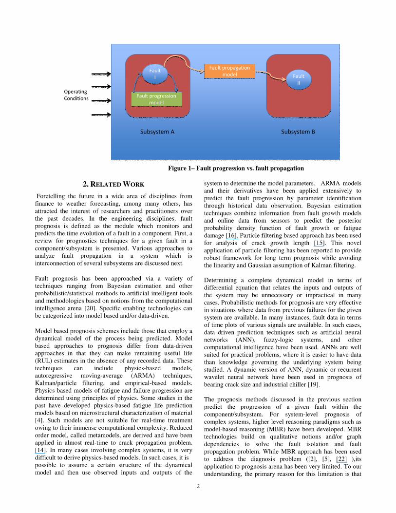
The progression of a fault condition and its effect on other components/subsystems is largely specific to the system. This paper focuses on developing a modular framework which could be applied to a variety of systems. In order to distinguish the fault evolution within a subsystem from spreading of effects of the fault to other subsystems, the former is hereafter referred to as fault progression/evolution and the latter as fault propagation. In Figure 1, a system consisting of two subsystems A and B is shown. An arbitrary fault, say fault I develops in the subsystem A. Fault progression aims at modeling evolution of fault I under given operating conditions/use strategy while fault propagation model estimates effect of fault I on another fault II in subsystem B. This paper aims at developing a methodology to analyze fault propagation only. The methodology is based on a modular structure with interdependent yet separate modules. Statistical design of experiments (DOE) techniques in conjunction with classical thermodynamics principles are used to construct these modules for a commercial turbofan engine.

2

Figure 1– Fault progression vs. fault propagation

2. RELATED WORK

Foretelling the future in a wide area of disciplines from finance to weather forecasting, among many others, has attracted the interest of researchers and practitioners over the past decades. In the engineering disciplines, fault prognosis is defined as the module which monitors and predicts the time evolution of a fault in a component. First, a review for prognostics techniques for a given fault in a component/subsystem is presented. Various approaches to analyze fault propagation in a system which is interconnection of several subsystems are discussed next.

Fault prognosis has been approached via a variety of techniques ranging from Bayesian estimation and other probabilistic/statistical methods to artificial intelligent tools and methodologies based on notions from the computational intelligence arena [20]. Specific enabling technologies can be categorized into model based and/or data-driven.

Model based prognosis schemes include those that employ a dynamical model of the process being predicted. Model based approaches to prognosis differ from data-driven approaches in that they can make remaining useful life (RUL) estimates in the absence of any recorded data. These techniques can include physics-based models, autoregressive moving-average (ARMA) techniques, Kalman/particle filtering, and empirical-based models. Physics-based models of fatigue and failure progression are determined using principles of physics. Some studies in the past have developed physics-based fatigue life prediction models based on microstructural characterization of material [4]. Such models are not suitable for real-time treatment owing to their immense computational complexity. Reduced order model, called metamodels, are derived and have been applied in almost real-time to crack propagation problem. [14]. In many cases involving complex systems, it is very difficult to derive physics-based models. In such cases, it is possible to assume a certain structure of the dynamical model and then use observed inputs and outputs of the

system to determine the model parameters. ARMA models and their derivatives have been applied extensively to predict the fault progression by parameter identification through historical data observation. Bayesian estimation techniques combine information from fault growth models and online data from sensors to predict the posterior probability density function of fault growth or fatigue damage [16]. Particle filtering based approach has been used for analysis of crack growth length [15]. This novel application of particle filtering has been reported to provide robust framework for long term prognosis while avoiding the linearity and Gaussian assumption of Kalman filtering. Determining a complete dynamical model in terms of differential equation that relates the inputs and outputs of the system may be unnecessary or impractical in many cases. Probabilistic methods for prognosis are very effective in situations where data from previous failures for the given system are available. In many instances, fault data in terms of time plots of various signals are available. In such cases, data driven prediction techniques such as artificial neural networks (ANN), fuzzy-logic systems, and other computational intelligence have been used. ANNs are well suited for practical problems, where it is easier to have data than knowledge governing the underlying system being studied. A dynamic version of ANN, dynamic or recurrent wavelet neural network have been used in prognosis of bearing crack size and industrial chiller [19]. The prognosis methods discussed in the previous section predict the progression of a given fault within the component/subsystem. For system-level prognosis of complex systems, higher level reasoning paradigms such as model-based reasoning (MBR) have been developed. MBR technologies build on qualitative notions and/or graph dependencies to solve the fault isolation and fault propagation problem. While MBR approach has been used to address the diagnosis problem ([2], [5], [22] ),its application to prognosis arena has been very limited. To our understanding, the primary reason for this limitation is that

Fault

I

Fault

I

Fault progression

model

Fault progression

model

Subsystem A

Operating

Conditions

Fault

II

Fault

II

Fault propagation

model

Fault propagation

model

Subsystem B

3

MBR approach builds on qualitative reasoning framework which is useful from fault isolation perspective but is of little utility in the field of prognostics. This is the same reason due to which root-cause analysis approaches find limited application in case of fault propagation analysis. Predicting the effect of occurrence of a fault in a component/subsystem on the other subsystems is inherently related to estimating the cause-and-effect relation between variables. Though, the first definition of causality which could be quantified and computationally measured, yet very general was given in 1956 by Wiener [21]. However, the introduction of concept of causality into experimental practice, namely into analysis of time series data, is due to Clive W.J. Granger, the 2003 Nobel Prize winner in economy [9]. Based on this concept, a non-parametric method for measuring causal information transfer between systems was proposed by Schreiber [18]. His transfer entropy concept is an information-theoretic functional of probability distribution functions. The Schreiber’s transfer entropy has found numerous applications in physiology [11], neurophysiology [3], financial data analysis [12] and in chemical plants [1]. The information-theoretic approaches to cause-and-effect estimation suffer from the drawback that they are based on multivariate probability distributions and hence, require a great amount of fault data. Bond graph is an energy-based graphical technique for building mathematical model of energy systems. Bond graphs models serve as knowledge representation of a large amount of structural, functional, and behavioral information and their relationship. This knowledge representation is used to create complex cause-effect reasoning leading to construction of powerful fault detection and isolation (FDI) systems [17]. Though various applications of bond graphs in diagnosis arena have been developed, a very little work has been done in applying this technique to prognostics. This paper aims at developing a methodology which is able to exploit physical relations between system variables to predict fault propagation in a system.

3. PROPOSED ARCHITECTURE

This paper proposes a modular algorithm to analyze fault propagation in a system. The proposed algorithm is based on architecture shown in figure 2. The architecture is populated with three interdependent yet separate models: a fault growth model, a stress model, and a feature model. Fault growth model

A system will fail when the applied load exceeds the strength of the product. The load can be voltage, current, temperature, or other variable. The load may be a onetime load or it may be applied a number of times. In the first case, overload failure will occur and in the second case

fatigue failure will occur. Consider applied load and strength plotted as shown in Figure 3a. The distance between load curve and strength curve is an indication of health of the system. As the system ages or a fault occurs in it, the strength curve moves to the left as depicted in Figure 3b. This movement of strength curve to the left is what is known as fault progression. Increased stresses result in an acceleration of movement of this curve. How various stresses affect progression of a fault: This relation between stress level and given fault condition is expressed by “fault growth model” in our proposed methodology.

Fault growth model determines time evolution of a given fault state x(t) under influence of stress vector u(t) as expressed in equation (1).

x•

(t) = f (t, x(t),u(t)) (1)

where x•

(t) is evolution of the given fault condition and

u(t) is stress vector which affects the fault evolution.

Feature model

Though there can be many state variables in any system, in the context of fault progression and fault evolution only those are of interest which would affect the dynamics of fault growth. For example, system internal temperature (state variable) will result in an increase in thermal stress and subsequently affecting fault progression. However, such state variables may depend on external operating conditions. This category of state variables is termed as feature vector in the subsequent paper and is cornerstone of this methodology. It is represented by y(t) in equation (2) and is modeled by g(.) as a function of external operating conditions z(t) and severity of the fault x(t).

))(),(()( tztxgty = (2)

Stress model

Fault progression is directly influenced by stresses. Typical stresses are high temperature, vibration, rate of change of temperature, humidity, power cycling (turning on/off),voltage variations. The stresses can come from two sources: external operating conditions (e.g. applied load) and system feature vector (e.g. system internal temperature). The relation between pertinent stresses and operating conditions and feature vector is modeled by stress model in the proposed methodology. In equation (3), h(.) represent the relation between stress vector u(t), external operating conditions z(t) and feature vector y(t).

))(),(()( tztyhtu = (3)

4

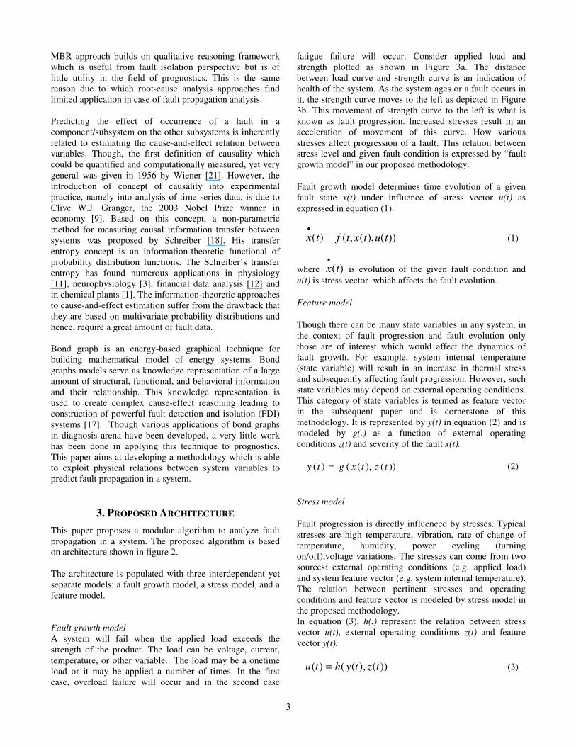
Figure 2– Architecture of the fault propagation algorithm

Fault propagation methodology

In a complex system such as an aircraft engine, there are several subsystems. Though each subsystem is an entity in itself, it is interacting with other subsystems too. Figure 2 represented architecture of fault propagation methodology for a system consisting of three subsystems, i.e., subsystem A, subsystem B and subsystem C. A fault condition exists in subsystem A. This fault condition is estimated as xA(t) by an independent diagnostic module. Two different feature models gA,B and gA,C determines appropriate features yA,B(t) and yA,C(t) which are then used to calculate stresses uB(t) and uC(t) for subsystems B and subsystem C respectively. This is mathematically expressed as

))(),(()( ,, tztxgty BABA = (4)

where xA(t) is given fault condition whose propagation effects we want to determine, z(t) is external operating condition vector and gA,B is feature model which yields feature yA,B(t) .

Stress model for subsystem B is expressed as

))(),(()( ,, tztyhtu BAABB = (5)

where ABh , determines stress vector )(tuB for a given fault

mode of system B. This stress vector subsequently determines evolution of fault xB through a fault growth model fB.

(6)

Thus, equations (4), (5), and (6), models effects of a fault xA from subsystem A to a fault xB in subsystem B. Fault growth model in our algorithm comes from physics of failure mechanism of the subsystem (in above case subsystem B). In most of the cases, this will be a stochastic model. Stress model relates external operating conditions and selected feature to the stresses. Principles of physics for the specific application domain will be involved in construction of the stress model. In the example presented in this paper, stress model is constructed by employing principles of thermodynamics. Feature model on the other hand is constructed by seeding faults in the system under a wide range of operating conditions

))(),(,()( tutxtftx BBBB =

•

Stresses uB(t)

yA,B(t)

Diagnostic ModelDiagnostic Model

Subsystem A

Fault growth model

Stress model

Feature model

x•

(t) = f (t, x(t), u(t))))(),(()( tztyhtu =))(),(()( ,, tztxgty BABA =

Subsystem B

Stresses uC(t)

x•

(t) = f (t, x(t), u(t))))(),(()( tztyhtu =

Subsystem C

yA,C(t)

))(),(()( ,, tztxgty CACA =

Stress model

Operating

Conditions

z(t)

xA(t)

)(tx B

•

)(txC

•

Fault growth model

Feature model

5

4. IMPLEMENTATION

The methodology discussed in the previous section was implemented on a turbofan aero-propulsion system. A recently released C-MAPSS [6] (Commercial Modular Aero Propulsion System Simulation) was used as simulation platform. C-MAPSS is well suited for our application because it

a) is a high fidelity model.

b) allows input variations of health related

parameters.

c) allows recording of large number of output sensor measurements.

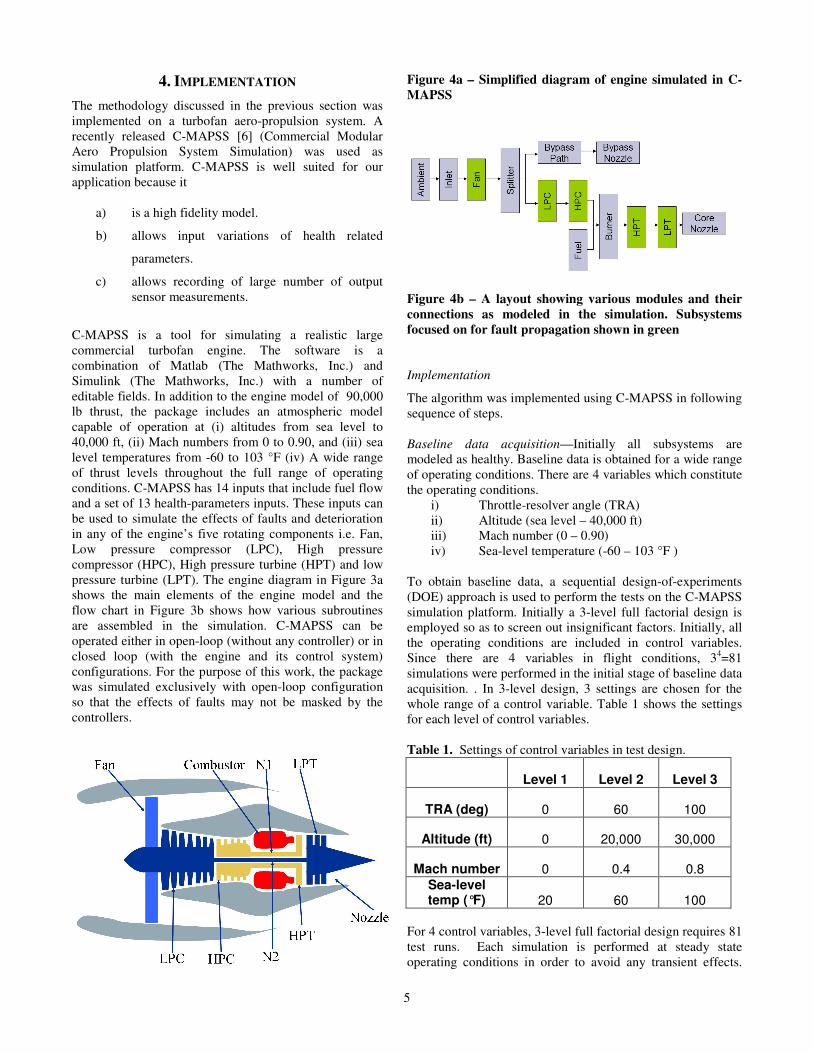
C-MAPSS is a tool for simulating a realistic large commercial turbofan engine. The software is a combination of Matlab (The Mathworks, Inc.) and Simulink (The Mathworks, Inc.) with a number of editable fields. In addition to the engine model of 90,000 lb thrust, the package includes an atmospheric model capable of operation at (i) altitudes from sea level to 40,000 ft, (ii) Mach numbers from 0 to 0.90, and (iii) sea level temperatures from -60 to 103 °F (iv) A wide range of thrust levels throughout the full range of operating conditions. C-MAPSS has 14 inputs that include fuel flow and a set of 13 health-parameters inputs. These inputs can be used to simulate the effects of faults and deterioration in any of the engine’s five rotating components i.e. Fan, Low pressure compressor (LPC), High pressure compressor (HPC), High pressure turbine (HPT) and low pressure turbine (LPT). The engine diagram in Figure 3a shows the main elements of the engine model and the flow chart in Figure 3b shows how various subroutines are assembled in the simulation. C-MAPSS can be operated either in open-loop (without any controller) or in closed loop (with the engine and its control system) configurations. For the purpose of this work, the package was simulated exclusively with open-loop configuration so that the effects of faults may not be masked by the controllers.

Figure 4a – Simplified diagram of engine simulated in C-

MAPSS

Figure 4b – A layout showing various modules and their

connections as modeled in the simulation. Subsystems

focused on for fault propagation shown in green

Implementation

The algorithm was implemented using C-MAPSS in following sequence of steps. Baseline data acquisition—Initially all subsystems are modeled as healthy. Baseline data is obtained for a wide range of operating conditions. There are 4 variables which constitute the operating conditions.

i) Throttle-resolver angle (TRA) ii) Altitude (sea level – 40,000 ft) iii) Mach number (0 – 0.90) iv) Sea-level temperature (-60 – 103 °F )

To obtain baseline data, a sequential design-of-experiments (DOE) approach is used to perform the tests on the C-MAPSS simulation platform. Initially a 3-level full factorial design is employed so as to screen out insignificant factors. Initially, all the operating conditions are included in control variables. Since there are 4 variables in flight conditions, 34=81 simulations were performed in the initial stage of baseline data acquisition. . In 3-level design, 3 settings are chosen for the whole range of a control variable. Table 1 shows the settings for each level of control variables. Table 1. Settings of control variables in test design.

Level 1 Level 2 Level 3

TRA (deg) 0 60 100

Altitude (ft) 0 20,000 30,000

Mach number 0 0.4 0.8 Sea-level temp (°F) 20 60 100

For 4 control variables, 3-level full factorial design requires 81 test runs. Each simulation is performed at steady state operating conditions in order to avoid any transient effects.

6

Data are recorded from 32 virtual sensors installed at various locations in the engine. These sensors monitor temperature, pressure, mass flow rate, torque, physical fan speed, and physical core speed at various locations in the engine. Fault data acquisition— Generally faults and deteriorations in turbine engines are modeled by adjusting independent parameters associated with each component. These parameters tend to shift the engine performance away from nominal. In the C-MAPSS engine model, there are 14 health parameter modifiers (Table 2) which allow the user to simulate faults and deterioration in any of the engine’s five rotating components (fan, LPC, HPC, HPT, and LPT). In this paper, HPC and HPT faults are focused on in order to give a proof of concept of the proposed methodology. These faults may have by definition safety-averse consequences such as loss of throttle control, compressor stalls, aborted takeoffs, in-flight shutdowns, etc. The HPC and HPT damage models are taken from experience based on the Navy SECAD program. Data and testing on the SECAD program validated that these faults can be modeled as changes to the flow and efficiency health parameters of the affected components [7]. Flow and efficiency health parameters of HPC and HPT are modified as representative of faults. HPC efficiency and HPT efficiency are modified by 2%. Efficiency modifier of 2% is regarded as a small fault in the fault model given by Goebel et al. [8]. Faults are seeded in HPC and HPT and system is simulated at the same levels of control variables as in baseline data acquisition phase. The same set of 32 sensors is used to record data at various locations in the system. Data analysis and feature selection— After acquiring baseline data and fault data, next step was to analyze these data so as to select a feature which could be used in the subsequent stages in the algorithm. Referring back to the algorithm architecture shown in Figure 2, feature is output of feature model and input to stress model. Selection criteria for feature vector in this case is somewhat similar to ‘feature selection’ in conventional fault diagnostics in a sense that in both cases the chosen parameter should give a reliable information about the fault level. However, in the case of fault propagation analysis, the feature vector should meet the following criteria (1) Feature vector should reveal fault state of the

faulty subsystem. (2) Feature vector should help in estimation of

stresses on the same or different subsystem. Obviously, there cannot exist any ubiquitous feature meeting these criteria for all of the fault modes of the system. However, we strive to choose a feature which could be applied to a variety of faults. In this paper,

exergy flow is proposed as such a parameter. It represents quantitatively the useful energy, or the ability to do or receive work i.e. the work content of variety of the streams (mass, heat, work) that flow through the system. An attribute of the property exergy is that it makes it possible to compare on a common basis different interactions (inputs, outputs, work, heat). Another benefit is that by accounting for all the exergy streams of the system it is possible to determine the extent to which the system destroys exergy. The destroyed exergy is proportional to the generated entropy, i.e. process irreversibilities in the system. In this work, it is assumed that for some of the fault modes, an increase in exergy destruction in a given subsystem is proportional to thermal stress acting on that subsystem. Validity of this assumption will depend on specific fault mode. Further investigations on this aspect of the assumption are part of the future work. In those cases, where this assumption is not valid, other parameters will be combined to come up with feature vector or an entirely different set of parameters may be used as feature vector. Table 2. C-MAPSS inputs to simulate various faults in any of the five rotating components of the engine.

Index Name

1 Fuel flow

2 Fan efficiency modifier

3 Fan flow modifier

4 Fan pressure-ratio modifier

5 LPC efficiency modifier

6 LPC flow modifier

7 LPC pressure-ratio modifier

8 HPC efficiency modifier

9 HPC flow modifier

10 HPC pressure-ratio modifier

11 HPT efficiency modifier

12 HPT flow modifier

13 LPT efficiency modifier

14 HPT flow modifier In this work, baseline data and fault data were imported into EES (Engineering Equation Solver- a thermodynamic analysis package) to calculate the exergy flow between different subsystems. Time rate of flow exergy for a control volume is calculated as [13]

]2

)()[(2

000 gzV

ssThhmf ++−−−=Ε

••

(7)

7

where f

•

Ε is time rate of flow exergy at the inlet or outlet

under consideration. •

m , h and s represents mass flow

rate, specific enthalpy, and specific entropy respectively

of the flowing stream. 2

2V

and gz accounts for kinetic

energy and potential energy while 0h and 0s denote

specific enthalpy and specific entropy, when the system is at equilibrium with the reference environment which is taken as a typical environmental condition of 1 atm and 25 °C. Stress estimation— As operating conditions change and/or fault condition arises in one of the subsystems, exergy flow between subsystems changes. This change in exergy flow results in a change in amount of the exergy destroyed in all the subsystems. Control volume exergy rate balance equation is expressed as

•••

−Ε−Ε+−−−=Ε

∑∑∑ d

e

fe

i

fiCV

CVj

j j

CV Edt

dVPWQ

T

T

dt

d)()1( 0

0

In the exergy rate balance equation, dt

d CVΕ represents the

time rate of change of the exergy of the control volume.

The term jQ•

represents the time rate of heat transfer at

the location on the boundary where the instantaneous temperature is Tj. The accompanying exergy transfer rate

is given by j

j

QT

T •

− )1( 0 . The term •

CVW represents the

time rate of energy transfer rate by work other than flow work. The accompanying exergy transfer rate is given by

)( 0dt

dVPW CV

CV −

•

, where dt

dVCV is the time rate of

change of volume. The terms fiΕ and feΕ accounts for

the time rate of exergy transfer accompanying mass flow and flow work at inlet i and exit e respectively. The time rates of exergy transfer terms are evaluated using equation

(7). Finally, the term •

dE accounts for the time rate of

exergy destruction due to irreversibilities within the control volume.

At steady-state, dt

d CVΕ=

dt

dVCV =0, so time rate of

exergy destruction can be expressed as

∑∑∑ Ε−Ε+−−=

•••

e

fe

i

fiCVj

j j

d WQT

TE )1( 0 (8)

Equation (8) was used to calculate rate of exergy destruction in all of the engine’s five rotating

components. As discussed previously, it was assumed that for some of the fault modes, exergy destruction in a system might be taken as a measure of thermal stress.

5. RESULTS AND DISCUSSION

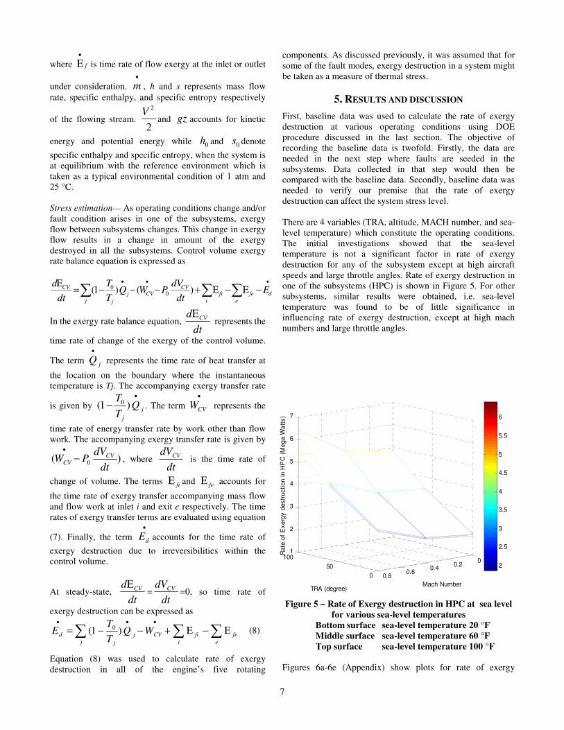
First, baseline data was used to calculate the rate of exergy destruction at various operating conditions using DOE procedure discussed in the last section. The objective of recording the baseline data is twofold. Firstly, the data are needed in the next step where faults are seeded in the subsystems. Data collected in that step would then be compared with the baseline data. Secondly, baseline data was needed to verify our premise that the rate of exergy destruction can affect the system stress level. There are 4 variables (TRA, altitude, MACH number, and sea-level temperature) which constitute the operating conditions. The initial investigations showed that the sea-level temperature is not a significant factor in rate of exergy destruction for any of the subsystem except at high aircraft speeds and large throttle angles. Rate of exergy destruction in one of the subsystems (HPC) is shown in Figure 5. For other subsystems, similar results were obtained, i.e. sea-level temperature was found to be of little significance in influencing rate of exergy destruction, except at high mach numbers and large throttle angles. Figure 5 – Rate of Exergy destruction in HPC at sea level

for various sea-level temperatures Bottom surface sea-level temperature 20 °F

Middle surface sea-level temperature 60 °F

Top surface sea-level temperature 100 °F

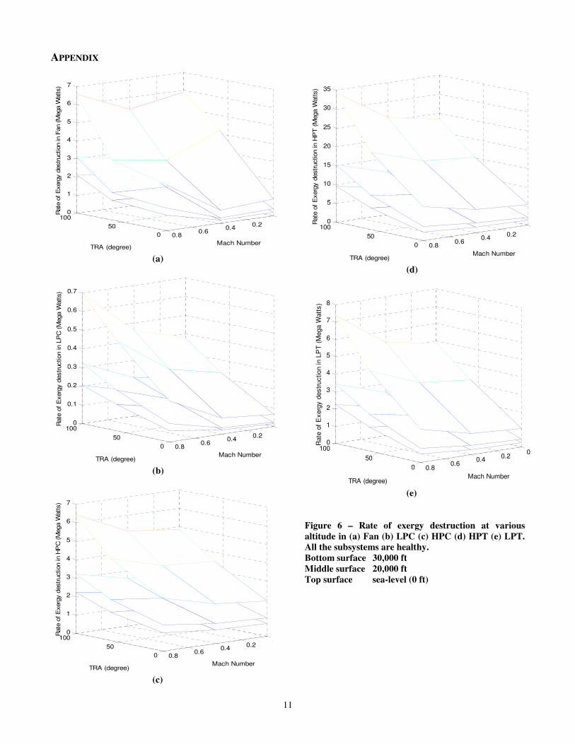
Figures 6a-6e (Appendix) show plots for rate of exergy

0

50

1000

0.20.4

0.60.8

1

2

3

4

5

6

7

Mach NumberTRA (degree)

Rate

of

Exerg

y d

estr

ucti

on in H

PC

(M

ega W

att

s)

2

2.5

3

3.5

4

4.5

5

5.5

6

8

destruction in fan, LPC, HPC, HPT, and LPT respectively, when aircraft operates at various altitudes. These plots show that the altitude is a significant factor in the rate of exergy destruction for all the subsystems. For baseline data (no fault in any subsystem), DOE results can be summarized as :

(1) Aircraft speed (Mach number) is a significant factor in the rate of exergy destruction which increases with an increase in aircraft speed.

(2) Throttle angle (TRA) is a significant factor in the rate of exergy destruction which increases with an increase in the throttle angle.

(3) Altitude is a significant factor in the rate of exergy destruction which decreases with the high altitudes.

(4) Sea-level temperature is relatively insignificant in rate of exergy destruction calculation except at high Mach numbers and large throttle angles.

The results obtained from baseline data conform to the assumption initially stated that the rate of exergy destruction might be an indicative of the system stress level. Intuitively, stress level should increase with high aircraft speed, high throttle power setting, or low altitude. The same is shown by the results obtained from baseline data i.e. the rate of exergy destruction in all components is largest at high aircraft speed, large throttle angle and low altitudes.

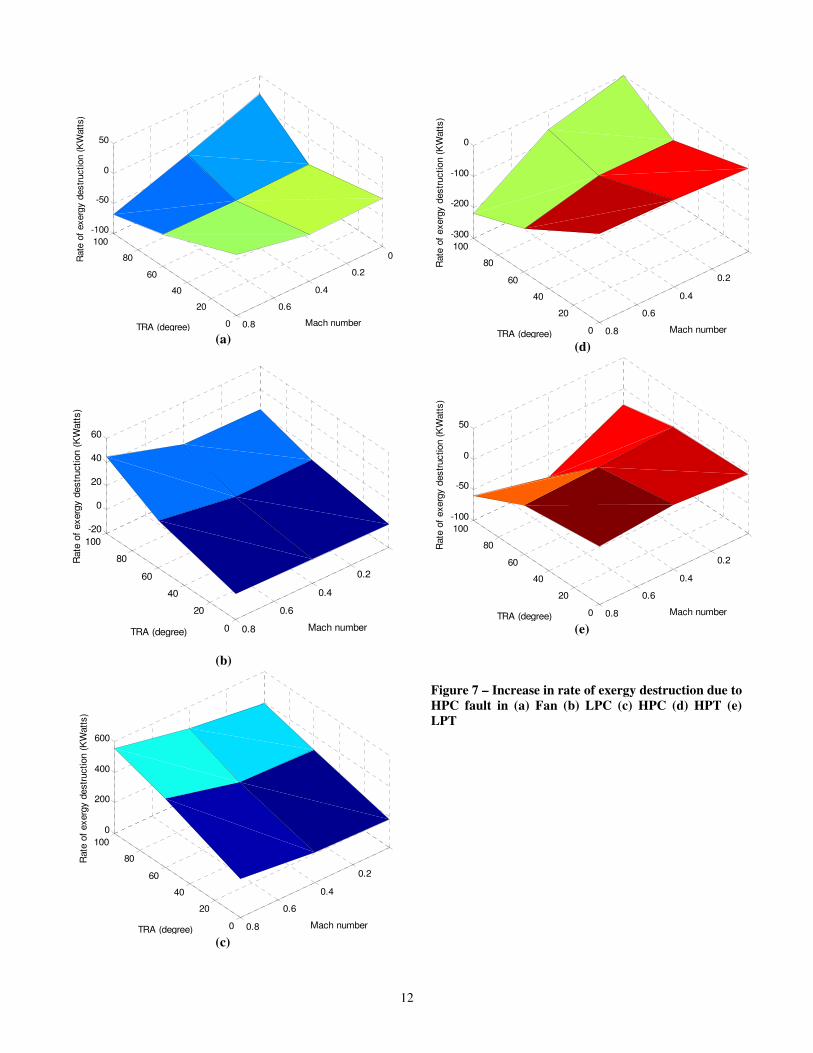
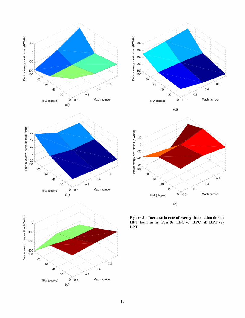
Figures 7a-7e (Appendix) show the increase in the rate of exergy destruction in the five rotating component due to an HPC fault and Figures 8a–8e (Appendix) show the increase in the rate of exergy destruction in the same components due to an HPT fault. It can be observed from these results that the largest increase in the rate of exergy destruction is in the same subsystem in which the fault is present. However, the other healthy subsystems also suffer a change in their rates of exergy destruction. Within these subsystems, the change is in a dissimilar fashion. For some of the subsystems, a fault in HPC causes an increase in their rate of exergy destruction while for others it decreases the rate of exergy destruction. The same is true for HPT fault as well. If the rate of exergy destruction in a subsystem is indicative of stress for a fault mode, it would increase chances of fault occurrence in that subsystem for which the exergy destruction rate has increased. These results qualitatively estimate the direction of fault propagation in the system. For example, the results show that HPC and HPT faults result in an increase in thermal stress on not only HPC and HPT respectively but also cause in a higher level of stress on LPC as well. How this stress actually translates into fault progression in these components, can

be quantified by incorporating fault growth models of the respective subsystems.

6. CONCLUSIONS

We presented a scheme to analyze fault propagation in a complex system. The scheme is based on modular architecture which breaks down fault propagation analysis procedure into separate modules. The scheme was implemented on an aeropropulsion system of turbofan type. A step by step procedure which involves DOE methods and thermodynamic analysis was laid out. Exergy destruction was used as a feature indicating thermal stress on the engine subsystems. Using this feature, flight conditions were translated into stress levels. Effect of occurrence of HPC and HPT faults on health of other subsystems was also qualitatively estimated.

The future work should focus on a specific engine with known material properties. A fault growth model should be built based on these properties. Then, the fault growth model should be integrated with the previously discussed qualitative stress analysis.

ACKNOWLEDGEMENT

The authors would like to thank Jonathan S. Litt in Glenn Research Center, NASA for providing valuable insight into the operation of C-MAPSS.

REFERENCES

[1] Bauer, M.; Cox, J. W.; Caveness, M. H.; Downs, J., Thornhill, N. F.., “Finding the Direction of Disturbance Propagation in a Chemical Process Using Transfer Entropy”, IEEE Trans. On Control Systems Technology, vol 15, Issue 1, Jan 2007.

[2] Buchina, G., and Clark, R. T., “AGETS MBR: An Application of Model-Based Reasoning for Advanced Diagnostics”, 1995 IEEE Aerospace Applications Conference Proceedings, vol. 2, issue 0, part 2, pp 169 – 180, Feb. 1995.

[3] M. Chávez, J. Martinerie, M. Le Van Quyen, Statistical assessment of nonlinear causality: application to epileptic EEG signals, J. Neurosci. Methods 124 (2003) 113–128.

[4] R. Friedman and H. L. Eidenoff, ‘‘A Two-Stage Fatigue Life Prediction Method,’’ Grumman Advanced Development Report, 1990, Bethpage, NY.

[5] Friedrich, G., Stumptner, M. and Wotawa, F., “Model-Based Diagnosis of Hardware Designs,” Artificial Intelligence, vol. 111, nos. 1–2, pp. 3–39, July 1999.

9

[6] D. Frederick, J. DeCastro, and J. Litt, "User’s Guide for the Commercial Modular Aero-Propulsion System Simulation (CMAPSS)," NASA/ARL, Technical Manual TM2007-215026, 2007.

[7] J. J. Gertler, “Survey of model based failure detection and isolation in complex plants,” IEEE Control Systems Magazine, pp. 1-1 1, December 1988.

[8] K. Goebel, H. Qiu, N. Eklund, and W. Yan, "Modeling Propagation of Gas Path Damage," in IEEE Aerospace Conference, Big Sky, MT, 2007.

[9] C.W.J. Granger, Time series analysis, cointegration, and applications. Nobel Lecture, December 8, 2003, in: Les Prix Nobel. The Nobel Prizes 2003, ed. Tore Frängsmyr, [Nobel Foundation], Stockholm, 2004, pp.360–366.

[10] Jordal K., Assadi M., Genrup M., "Variations in Gas-Turbine Blade Life and Cost due to Compressor Fouling - a Thermoeconomic Approach", International Journal of Applied Thremodynamics, March 2002.

[11] T. Katura, N. Tanaka, A. Obata, H. Sato, A. Maki, Quantitative evaluation of interrelations between spontaneous low-frequency oscillations in cerebral hemodynamics and systemic cardiovascular dynamics, Neuroimage 31 (2006) 1592–1600.

[12] R. Marschinski, H. Kantz, Analysing the information flow between financial time series—an improved estimator for transfer entropy, Eur. Phys. J. B 30 (2002) 275–281.

[13] M. J. Moran and H. N. Shapiro, Fundamentals of Engineering Thermodynamics, John Wiley, 2004.

[14] J. C. Newman, ‘‘FASTRAN-II: A Fatigue Crack Growth Structural Analysis Program,’’NASA Technical Memorandum, 1992 Langley Research Center, Hampton, VA.

[15] M. Orchard, B. Wu, and G. Vachtsevanos, ‘‘A Particle Filter Framework for Failure Prognosis,’’ Proceedings of WTC2005, World Tribology Congress III, Washington, DC, 2005.

[16] Przytula, K. W. and Thompson, D., “Construction of Bayesian Networks for Diagnostics”, 2000 IEEE Aerospace Conference Proceedings, vol. 5, pp. 193 - 200, March 2000.

[17] Samantaray A. K., Ghoshal S. K, "Sensitivity bond graph approach to multiple fault isolation through parameter estimation", Proceedings of the I MECH E Part I Journal of Systems & Control Engineering,, March 2002.

[18] T. Schreiber, Measuring information transfer, Phys. Rev. Lett. 85 (2000) 461–464.

[19] F. C. Tsui, M. G. Sun, C. C. Li, and R. J. Sclabassi, ‘‘A Wavelet-Based Neural Network for Prediction of ICP Signal,’’ Proceedings of IEEE Engineering in Medicine and Biology, Vol. 2. Montreal, Canada IEEE 1995, pp. 1045–1046.

[20] Vachtsevanos G., F. L. Lewis, M. J. Roemer, A. Hess, B. Wu, Intelligent Fault Diagnosis and Prognosis for Engineering Systems, John Wiley and Sons, 2006.

[21] N.Wiener, The theory of prediction, in: E.F. Beckenbach (Ed.), Modern Mathematics for Engineers, McGraw-Hill, NewYork, 1956.

[22] Wu B., Saxena A., Khawaja T. S., Patrick R., Vachtsevanos G., and Spari P., “An Approach to Fault Diagnosis of Helicopter Planetary Gears”, IEEE AUTOTESTCON 2004 Proceedings, pp 475 – 481, Sep. 2004.

BIOGRAPHY

Manzar Abbas earned the B.E.

degree from the National University

of Sciences and Technology (NUST),

Pakistan in 1999 and the Masters of

Electrical Engineering from the

Georgia Institute of Technology in

2007. He joined intelligent control

systems laboratory(ICSL) in summer

2005 and is currently a Ph.D.

candidate in Electrical Engineering

at the Georgia Institute of

Technology .In the past, he carried out applied research in the

areas of fault diagnostics and failure prognostics of electrical,

electrochemical, electromechanical and electronics systems.

Currently, he is working on developing a methodology to

analyze fault propagation from one subsystem to the other

subsystems with a specific focus on turbo machinery.

George Vachtsevanos is a Professor

Emeritus of Electrical and Computer

Engineering at the Georgia Institute

of Technology. He was awarded a

B.E.E. degree from the City College

of New York in 1962, a M.E.E. degree

from New York University in 1963

and the Ph.D. degree in Electrical

Engineering from the City University

of New York in 1970. He directs the

Intelligent Control Systems

laboratory at Georgia Tech where faculty and students are

10

conducting research in intelligent control,

neurotechnology and cardiotechnology, fault diagnosis

and prognosis of large-scale dynamical systems and

control technologies for Unmanned Aerial Vehicles. His

work is funded by government agencies and industry. He

has published over 240 technical papers and is a senior

member of IEEE. Dr. Vachtsevanos was awarded the

IEEE Control Systems Magazine Outstanding Paper

Award for the years 2002-2003 (with L. Wills and B.

Heck). He was also awarded the 2002-2003 Georgia

Tech School of Electrical and Computer Engineering

Distinguished Professor Award and the 2003-2004

Georgia Institute of Technology Outstanding

Interdisciplinary Activities Award.

–

11

APPENDIX

0

50

1000

0.20.4

0.60.8

0

1

2

3

4

5

6

7

Mach NumberTRA (degree)

Rate

of E

xerg

y d

estruction in F

an (M

ega W

atts)

(a)

0

50

1000

0.20.4

0.60.8

0

0.1

0.2

0.3

0.4

0.5

0.6

0.7

Mach NumberTRA (degree)

Rate

of

Exerg

y d

estr

uction in L

PC

(M

ega W

att

s)

(b)

0

50

1000

0.20.4

0.60.8

0

1

2

3

4

5

6

7

Mach NumberTRA (degree)

Rate

of E

xerg

y d

estr

uction in H

PC

(M

ega W

att

s)

(c)

0

50

1000

0.20.4

0.60.8

0

5

10

15

20

25

30

35

Mach NumberTRA (degree)

Rate

of

Exerg

y d

estr

uction in H

PT

(M

ega W

att

s)

(d)

0

50

1000

0.20.4

0.60.8

0

1

2

3

4

5

6

7

8

Mach NumberTRA (degree)

Rate

of

Exerg

y d

estr

uction in L

PT

(M

ega W

att

s)

(e)

Figure 6 – Rate of exergy destruction at various

altitude in (a) Fan (b) LPC (c) HPC (d) HPT (e) LPT.

All the subsystems are healthy.

Bottom surface 30,000 ft

Middle surface 20,000 ft

Top surface sea-level (0 ft)

12

0

20

40

60

80

100

0

0.2

0.4

0.6

0.8

-100

-50

0

50

Mach numberTRA (degree)

Rate

of

exerg

y d

estr

uction (

KW

att

s)

(a)

0

20

40

60

80

100

0

0.2

0.4

0.6

0.8

-20

0

20

40

60

Mach numberTRA (degree)

Rate

of

exerg

y d

estr

uction (

KW

att

s)

(b)

0

20

40

60

80

100

0

0.2

0.4

0.6

0.8

0

200

400

600

Mach numberTRA (degree)

Rate

of

exerg

y d

estr

uction (

KW

att

s)

(c)

0

20

40

60

80

100

0

0.2

0.4

0.6

0.8

-300

-200

-100

0

Mach numberTRA (degree)

Rate

of

exerg

y d

estr

uction (

KW

att

s)

(d)

0

20

40

60

80

100

0

0.2

0.4

0.6

0.8

-100

-50

0

50

Mach numberTRA (degree)

Rate

of

exerg

y d

estr

uction (

KW

att

s)

(e)

Figure 7 – Increase in rate of exergy destruction due to

HPC fault in (a) Fan (b) LPC (c) HPC (d) HPT (e)

LPT

13

0

20

40

60

80

100

0

0.2

0.4

0.6

0.8

-100

-50

0

50

Mach numberTRA (degree)

Rate

of

exerg

y d

estr

uction (

KW

att

s)

(a)

0

20

40

60

80

100

0

0.2

0.4

0.6

0.8

-20

0

20

40

60

Mach numberTRA (degree)

Rate

of

exerg

y d

estr

uction (

KW

att

s)

(b)

0

20

40

60

80

100

0

0.2

0.4

0.6

0.8

-300

-200

-100

0

Mach numberTRA (degree)

Rate

of

exerg

y d

estr

uction (

KW

att

s)

(c)

0

20

40

60

80

100

0

0.2

0.4

0.6

0.8

100

200

300

400

500

Mach numberTRA (degree)

Rate

of

exerg

y d

estr

uction (

KW

att

s)

(d)

0

20

40

60

80

100

0

0.2

0.4

0.6

0.8

-60

-40

-20

0

20

Mach numberTRA (degree)

Rate

of

exerg

y d

estr

uction (

KW

att

s)

(e) Figure 8 – Increase in rate of exergy destruction due to

HPT fault in (a) Fan (b) LPC (c) HPC (d) HPT (e)

LPT