1

An Effective AHP based Metaheuristic Approach to Solve

Supplier Selection Problem

Tamal Ghosh1, Tanmoy Chakraborty, Pranab K Dan

Department of Industrial Engineering & Management,

West Bengal University of Technology.

BF 142, Sector 1, Salt Lake City, Kolkata 700064, India.

Email: tamal.31@gmail.com, chakrabortytanmoy.85@gmail.com, danpk.wbut@gmail.com.

Abstract

The supplier selection problem is based on electing the best supplier from a group of pre-

specified candidates, is identified as a Multi Criteria Decision Making (MCDM), is

proportionately significant in terms of qualitative and quantitative attributes. It is a

fundamental issue to achieve a trade-off between such quantifiable and unquantifiable

attributes with an aim to accomplish the best solution to the abovementioned problem. This

article portrays a metaheuristic based optimization model to solve this NP-Complete problem.

Initially the Analytic Hierarchy Process (AHP) is implemented to generate an initial feasible

solution of the problem. Thereafter a Simulated Annealing (SA) algorithm is exploited to

improve the quality of the obtained solution. The Taguchi robust design method is exploited

to solve the critical issues on the subject of the parameter selection of the SA technique. In

order to verify the proposed methodology the numerical results are demonstrated based on

tangible industry data.

Keywords: supplier rating; vendor section; AHP; simulated annealing; metaheuristic;

Taguchi method.

1. Introduction

Over the decades the supplier selection problem has been dragging the attention of the researchers and

practitioners in the vicinity of Supply Chain Management study. Therefore several techniques have

been proposed by the academicians and professionals to solve this Multi Criteria Decision Making

(MCDM) problem. As Dickson (1966) stated that contemporary firms have the alternatives to select a

suitable technique to decipher the complicated job of selecting suppliers. These techniques varies

from the adoption of uncomplicated methods such as the selection of the vendor offering lowermost

tender to the effective complicated methods which exploit the unquantifiable attributes of the supplier

selection problem. Although many empirical studies are already contributed in the proposed area of

research, yet the researchers and practitioners are involved in improving the solution methodologies

due to the involvement of growing complexities of technology innovation. In manufacturing industry

the procurement cost of raw materials from the outside suppliers and the other unquantifiable

attributes such as quality of the materials delivered and the time of delivery are substantially crucial

and nearly 70% to 80% of the total cost involved in the whole product development phase (Weber,

1 Corresponding Author: Email: tamal.31@gmail.com, Phone: +91-33-2334-1014, Fax: +91-33-2334-1031.

2

Current and Benton, 1991). Since the early 1990’s a set of hard to estimate unquantifiable attributes

have turned out to be the key components of the supplier selection problem which further helped in

developing novel and complicated methodologies (Ellram, 1990). Selecting an optimal set of

suppliers on this basis certainly increase the sustainability of the firms in present global competition

(Thompson, 1990). Traditionally the supplier selection problem is based on the purchasing cost,

quality and delivery functionality of the raw materials. Consideration of the above aspects enhances

the complexities of the problem in polynomial time. The selection decision becomes extensively

significant for any person-in-charge of the procurement department due to the several different levels

of success of the rival suppliers under these stated circumstances (Aissaoui, Haouari and Hassini,

2007). The vendor with the lowermost tender might not be the best in delivering the material of

proper quality. In case of the government bodies, the practice of decision-making optimization model

in vendor selection processes would be extremely helpful than the private firms. In the government

framework, there is a legal need to obey the formal rules and procedures that control vendor selection

processes. Therefore such decision models could be immensely supportive in maintaining

transparency and doing fair business (Schooner, 2003). It is evident from the past literature that the

precise and sophisticated methodologies are urgently required to solve the supplier selection problems

(Scott, 1995). For that matter Kanagaraj and Jawahar (2009) have implemented a Simulated

Annealing Algorithm (SAA) tool for supplier selection problems to obtain the optimal or near-optimal

solutions quickly. Saen (2009) introduced a technique based on Data Envelopment Analysis (DEA) to

rank the suppliers in the presence of nondiscretionary factors. An integrated model of Fuzzy-AHP and

decision support system was proposed by Gnanasekaran, Velappan and Manimaran (2010) for

supplier selection to reduce the cost and enhance the product quality with the help of the Reliability-

Based Total Cost of Ownership (RBTCO) model. This integrates purchasing, maintenance and

stoppage costs along with the realistic constraints based on product reliability and weight restraint.

Nonlinear Integer Programming (NLIP) is used to develop the mathematical formulation of the

RBTCO model.

In present article a multiobjective supplier selection problem has been introduced which has

incorporated faulty materials and delay in delivery cost as decisive factors. Thereafter a Simulated

Annealing (SA) based optimization model is implemented to solve this problem. The initial solution

to the SA procedure is generated using Analytic Hierarchy Process (AHP). In order to select the

optimal set of parameters to the SA, Taguchi’s Design of Experiments (DOE) technique is exploited.

The rest of the article is structured in following manner, section 2 presents a brief literature survey of

the proposed area of study, section 3 demonstrates the formulation of the proposed multiobjective

problem model, section 4 elaborates the proposed solution methodology and numerical results are

depicted in section 5 followed by the managerial implications and conclusion of this research.

2. Literature Survey

Li, Fun and Hung (1997) reported that the supplier selection methodologies are practiced to facilitate

the selection process which further have a substantial impact on the selection outcomes. Numerous

supplier selection methods have been established and categorized over the decades. Petroni and

Braglia (2000) proposed linear weighting method using supplier rating based on different attributes

which is a faster and inexpensive method to instigate. Although various drawbacks and limitations are

also indicated in their study. Cost proportion (Timmerman, 1986) and aggregate cost of proprietorship

(Ellram, 1990) based on aggregate cost approaches assemble all the cost components of the supplier

selection process in fiscal units which are very flexible methods. These are exact methods and due to

the complexities and time involvement these methods are moderately expensive to implement.

Mathematical programming approaches primarily exploit the quantifiable factors; these approaches

3

comprise the Principal Component Analysis (PCA) (Petroni and Braglia, 2000) and the Artificial

Neural Network (ANN) (Choy, Lee and Low, 2002). Bello (2003) stated in his research that the PCA

approach is advantageous in terms of its competency in managing various differing aspects. The ANN

approaches are also useful in cost minimization and time reduction.

Multiple Attribute Utility Theory method is practiced for global vendor selection problems, in which

the surroundings are more complex and uncertain (Zhao and Bross, 2004). Chen, Lin and Huang

(2006) demonstrated that the Fuzzy set theory technique controls such situations for supplier

performance evaluation. The approach is helpful to the managers to purchase from the suppliers

according to their own choice. a fuzzy weighted additive and mixed integer linear programming is

developed. The model aggregates weighted membership functions of objectives to construct the

relevant decision functions, in which objectives have different relative importance. Ng (2008)

proposed a weighted linear program for the supplier selection problem. This paper demonstrates a

transformation technique with the mathematical model which can solve the problem without an

optimizer. Amid, Ghodsypour and O’Brien (2009) demonstrated fuzzy multiobjective and additive

model to consider the imprecision of information along with the order quantities to each supplier

using price breaks. The objective functions used are, minimizing the net cost, rejected items and late

deliveries, while satisfying other constraints such as capacity and demand requirement. Authors

further stated weighted max–min model in the similar problem environment (Amid, Ghodsypour and

O’Brien, 2010) with the help of Analytic Hierarchy Process (AHP). The proposed model could be

utilized to find out the appropriate order to each supplier. Saen and Zohrehbandian (2008) proposed

DEA approach with quantity discount policy to select the best supplier. Wu (2009) stated a hybrid

model using data envelopment analysis (DEA), decision trees (DT) and neural networks (NNs) to

evaluate supplier performance. The model comprised of two parts. The first part utilized DEA and

categorizes the suppliers into several clusters thereafter the second part used the performance-related

data of the company to train decision trees and intelligent neuro model, the precised results are

obtained. However Saen (2008) stated an approach based on super-efficiency analysis based on DEA

to rank the suppliers in presence of volume discounts. Author further proposed another DEA based

method to rank the suppliers in the presence of weight limitations and dual-role factors (Saen, 2010).

The Analytical Hierarchical Process (AHP) is the most exploited method in supplier selection

problems, which is a Multi Criteria Decision Making technique. It is implemented to rank the

alternatives when several criteria are believed to be considered and it permits the managers to

formulate complicated problems in the form of a hierarchical relationship (Saaty, 1980). The AHP is

comparatively straightforward method to practice. This technique integrates tangible and intangible

attribute of the problems. A detail survey (Tahriri et al., 2008) of the supplier selection methods

portrays that the AHP is the most frequently employed method in supplier selection. The AHP

hierarchy typically contains three distinct levels, which are objectives, factors, and alternatives. AHP

suggests an way to rank the alternative choices based on the manager’s decisions relating the

significance of the criteria. Due to this fact AHP is preferably appropriate for the abovementioned

problem. The problem hierarchy provides itself to an analysis based on the impact of a given level on

the next higher level (Saaty, 1980). Managerial judgments are stated in terms of the pair-wise

comparisons of entries on a specified level of the hierarchy based on their influences on the next

higher level. Each of the pair-wise comparisons signifies an approximation of the proportion of the

weights of the two criteria being compared. Since AHP exploits a proportionate scale for personal

decisions, the relative weights reflect the relative importance of the norms in attaining the objective of

the hierarchy (Tam and Tummala, 2001). Yahya and Kingsman (1990) used Saaty’s AHP method to

determine primacy in selecting suppliers. The authors employed vendor rating in determining how to

allot business and where inadequate progress work is utilized. Akarte (2001); Handfield, Walton and

4

Sroufe (2002); Yu and Jing (2004); Liu and Hai (2005); Rajkumar, Kannan and Jayabalan (2009) also

utilized AHP technique in their study as an integral part.

Most of the supplier selection literature generally used traditional methods. Traditional techniques are

not efficient when the solution state space is large and various constraints cause the vendor selection

problem more complicated. Very few articles utilized state-of-the-art methods such as metaheuristics.

Recently Arunkumar, Karunamoorthy and Makeshwaraa, (2007); Rezaei and Davoodi (2008); Kubat,

and Yuce, (2006); Ding, Benyoucef and Xie (2003) have proposed Genetic Algorithm based

metaheuristic approach to solve supplier selection problems in multiobjective environment.

This present research introduces an efficient metaheuristic approach based on Simulated Annealing to

solve the supplier selection problem.

3. Problem Formulation

Supplier selection processes are primarily reliant on the specific objectives being solved with the

problem and the relevant constraints related to the objectives. In this article a case of a Leading

construction firm of India has been considered to derive the multiobjective optimization model. This

firm constructs commercial buildings as well as residential units in large scale such as IT/ITeS SEZ,

Shopping malls, hospitality and retail units, logistics and industrial squares etc. Due to the heavy

construction approach, this company requires various raw materials such as steel beams, cement, light

weight bricks, cast iron etc.

The proposed model is articulated considering the constrictions which are managed rationally by this

firm to select suppliers. Each raw material supplied by the supplier would have different constraints

and characteristics such as percentage of faulty materials supplied, percentage delay in delivery and

unit purchasing cost of the materials. Each supplier certainly has its own capacity to supply. The firm

has specific requirements of material in certain period. If raw material j is being supplied by supplier

k, then the initial procurement cost is defined as,

𝑃𝑐 = ∑ ∑ 𝜑𝑗𝑘𝑞𝑗𝑘

𝑁

𝑘=1

𝑀

𝑗=1

(1)

where

φjk is the unit cost of jth material supplied by kth supplier.

qjk is the amount of material type j procured by ith supplier.

The total substandard delivery is defined as,

𝑄𝑑 = ∑ ∑ 𝛿𝑗𝑘𝑞𝑗𝑘

𝑁

𝑘=1

𝑀

𝑗=1

(2)

where

δjk is the percentage of faulty items of jth material supplied by kth supplier.

qjk is the amount of material type j procured by ith supplier.

The total delay in delivery is defined as,

5

𝐷𝑑 = ∑ ∑ 𝜃𝑗𝑘𝑞𝑗𝑘

𝑁

𝑘=1

𝑀

𝑗=1

(3)

where

θjk is the delay percentage in delivery of jth material supplied by kth supplier.

qjk is the amount of material type j, procured by ith supplier.

In this supplier selection problem three objectives are simultaneously considered, (i) to minimize the

total procurement cost, (ii) to minimize the total number of faulty items supplied and (iii) to minimize

the total number of delay days in delivery in procuring various raw materials from various suppliers.

The quality function (2) demonstrates the number of faulty items supplied by the suppliers. The faulty

items are generally detected by the receiving firm while relocating the raw materials to the inventory.

The firm’s strategy is to return back the substandard items to the suppliers and request them to replace

those items within stipulated time which is substantially one week. Therefore in a project under fixed

schedule, supply of substandard material could incur the total cost in terms of one week delay time.

Thus the quality function of equation (2) and total delay in delivery of equation (3) could be

transformed into a non-compliance cost component using,

𝑄𝑐 = (7 + 𝐷𝑑) × 𝐶𝑑 (4)

Hence the proposed multiobjective model aims in minimizing the total cost function f(x),

𝑀𝑖𝑛𝑖𝑚𝑖𝑧𝑒 𝑓(𝑥) = 𝑃𝑐 + 𝑄𝑐 (5)

subject to

𝑞𝑗𝑘 ≤ 𝑋𝑗𝑘 (6)

∑ 𝑞𝑗𝑘

𝑁

𝑘=1

≥ 𝑌𝑗 (7)

where

Xjk is the capacity of supplier k while supplying material j

Yjk is the demand of material j to the firm in certain period

Constraint (6) confirms that each supplier supplies according to its capacity. Constraint (7) confirms

that total raw material procured should harmonize the firm’s demand. This proposed multiobjective

model is validated using simulated annealing (SA) approach by considering these abovementioned

objectives and constraints which further gives the optimal selection results of suppliers. In order to

define the SA approach, a quick solution generation method is believed to be identified and the

generated feasible solution is assumed to be used as the initial solution to the SA algorithm. Therefore

in this research Analytic Hierarchy Process (AHP) is utilized to serve the purpose. The next section

would demonstrate the details of the solution methodologies involved in this approach.

6

4. Research Methodology

To facilitate the present research work authors have visited an eminent construction firm operating in

Kolkata, India. Currently the firm is involved in a big project based on development of an IT/ITeS

Special Economic Zone (SEZ) in sector V, Rajarhat, Newtown in Salt Lake City Kolkata. Authors

have prepared the questionnaires based on the information gathered from the professionals of the

abovementioned firm. On the basis of the experts opinion the AHP analysis has been carried out in

this study.

The proposed optimization methodology is developed using Simulated Annealing (SA) algorithm to

achieve the optimal solutions. The SA algorithm simulates the natural annealing process, where

particles of a solid organize themselves into a thermal equilibrium. An introduction to SA can be

obtained from the book by Aarts and Korst (1990). The general applications concerns combinatorial

optimization problems of the following form where S is a predetermined set of feasible solutions.

minx∈S g(x) (8)

The algorithm exploits a pre-defined neighbourhood structure on ‘S’. A control parameter called

temperature in resemblance to the natural annealing process governs the search behaviour. In each

iteration, a neighbour solution y to the current solution x is figured out. If y has an improved objective

function value than x, the solution y is accepted, that is, the current solution x is swapped by y.

Alternatively if y does not attain a better objective function value than x, the solution y is only

recognized with a specific probability depending on (i) the difference of the objective function values

in x and y, and (ii) the temperature parameter. The pseudocode below exhibits the general SA method.

Pseudocode (SA)

initialize;

repeat

generate a candidate solution;

evaluate the candidate;

determine the current solution;

reduce the temperature;

until termination condition is met;

In this article, factors which affect the decision makers’ strength are analysed. The process follows

these steps,

Using the AHP method, the weight of the factors are obtained from qualitative expressions

and each supplier’s weight is also achieved and final composite criteria weights are

determined by AHP. This further rank the suppliers according to their composite scores.

Therefore according to the ranks the suppliers could be selected.

Simulated Annealing (SA) takes the ranks obtained from previous step and attempts to search

for optimal set of suppliers based on the objectives defined in section 3.

4.1. Initial Solution Generation

In this article AHP is exploited to select initial set of suppliers. This solution is an initial feasible

solution to the SA method based optimization model.

7

4.2. Analytical Hierarchy Process (AHP)

The AHP is a multi-criteria decision technique that exploits hierarchical relationships to represent a

problem. Primacies for substitutes are acquired based on the opinion of the experts (Saaty, 1980). The

method consists of several important steps: outlining the shapeless problem into shape, obtaining the

AHP hierarchical relationships, forming pairwise comparison matrices, approximating the relative

weights, examining the consistency and finally attaining the overall ranking (Lee, Chen and Chang,

2008). AHP can empower managers to represent the interface of several factors in complicated and

shapeless circumstances. The technique is based on the pairwise comparison of decision variables

with respect to the factors or substitutes. A pairwise comparison matrix is obtained of size n×n, where

n is the number of criteria to be compared. The AHP method is adopted in this article is stated as,

Step 1: The hierarchical relationship of the problem is obtained and presented in Figure 1. The

proposed AHP method decomposes the problem into three levels (Saaty, 1980): (i)The first level

demonstrates the main objective: the selection of suppliers, the second level depicts the criteria and

the last level reports the six suppliers to be compared.

Figure 1. Hierarchical relationship of the supplier selection problem

Step 2: Calculation of the pairwise comparison matrix for each level is required. For the pairwise

comparison, a ranking scale is used for the criteria evaluation (Saaty, 1980). The scale is a crisp scale

ranging from 1 to 9, as presented in Table 1. This scale values are assigned to the criteria based on the

experts opinion of the AHP questionnaire sheet prepared by the authors. The pairwise comparison

matrix for all the criteria is presented in Table 2. The last column of table 2 depicts the overall

importance of the criteria over each other.

The AHP procedure is presented as,

Consider [Ax = λmaxx] where

A is the comparison matrix of size n×n, for n criteria.

x is the Eigenvector of size n×1

λmax is the Eigenvalue, λmax > n.

To find the ranking of priorities, namely the Eigen Vector X:

1. Initialization:

1.1. Take the squared power of matrix A, i.e., A2=A×A

1.2. Find the row sums of A2 and normalize this array to find E0.

1.3. Set A:=A2

8

2. Main:

2.1. Take the squared power of matrix A, i.e., A2=A×A

2.2. Find the row sums of A2 and normalize this array to find E1.

2.3. Find D= E1 - E0.

2.4. If the elements of D are close to zero, then X= E1

2.5. else set A:=A2 , set E0:=E1 and go to Step 2.1.

2.6. STOP.

Table 1. Saaty’s 9 point scale

Importance Value Definition Description

1 Equal Strong Two factors are equally Contributing to objective

3 Moderate Strong One factor is marginally superior over other

5 Fairly Strong One factor is strongly superior over other

7 Very Strong One factor is very stongly superior over other

9 Absolute Strong The highest level of superiority of one factor over other

2, 4, 6, 8 Intermediate Values According to the negotiation required

Table 2. Comparison matrix of main attributes

Table 3 to Table 5 present the pairwise comparison matrices of the suppliers with each of the criteria

selected in this research. The last columns of pairwise matrices present the calculated relative weights

of the suppliers over each other.

Table 3. Pairwise comparison matrix of suppliers with respect to cost

S1 S2 S3 S4 S5 S6 Relative Weight

S1 1 3 2 7 6 5 0.40201

S2 1/3 1 1/2 5 4 3 0.18549

S3 1/2 2 1 4 3 2 0.21024

S4 1/7 1/5 1/3 1 1/2 1/4 0.03831

S5 1/6 1/4 1/3 2 1 1/3 0.05611

S6 1/5 1/3 1/2 4 3 1 0.10786

Table 4. Pairwise comparison matrix of suppliers with respect to quality

S1 S2 S3 S4 S5 S6 Relative Weight

S1 1 3 5 1/3 7 8 0.26949

S2 1/3 1 4 1/4 5 7 0.15914

S3 1/5 1/4 1 1/5 3 4 0.07354

S4 3 4 5 1 8 9 0.43202

S5 1/7 1/5 1/3 1/8 1 3 0.04087

S6 1/8 1/7 1/4 1/9 1/3 1 0.02493

Cost Quality Delivery Relative Weight (PV)

Cost 1 1/5 1/9 0.062941

Quality 5 1 1/3 0.265433

Delivery 9 3 1 0.671625

9

Table 5. Pairwise comparison matrix of suppliers with respect to delivery

S1 S2 S3 S4 S5 S6 Relative Weight

S1 1 5 2 1/3 6 7 O.26324

S2 1/5 1 2 1/4 3 4 0.11631

S3 1/2 1/2 1 1/5 3 5 0.10426

S4 3 4 5 1 7 9 0.43627

S5 1/6 1/3 1/3 1/7 1 4 0.05268

S6 1/7 1/4 1/5 1/9 1/4 1 0.02723

The overall rating of each supplier is computed by adding the product of the relative weight of each

criterion and the relative weights of the suppliers considering the corresponding criteria (Table 6).

Table 6 demonstrates that supplier 4 (overall ranking is 1 and composite score is 0.4099) is the best

supplier followed by supplier 1, 2, 3, 5 and 6.

4.3 Computation of consistency index and consistency ratio

AHP procedure requires the computation of consistency ratio to ensure the precision of the obtained

solution. The consistency index (CI) of pairwise comparison matrix is calculated using,

𝐶𝐼 =𝜆𝑚𝑎𝑥 − 𝑛

𝑛 − 1 (9)

and the random consistency index (RI) is computed as,

𝑅𝐼 = 1.98𝑛 − 2

𝑛 (10)

where λmax is the maximum eigenvalue and n is the size of pairwise comparison matrix. Thus the

consistency ratio (CR) is obtained using,

𝐶𝑅 =𝐶𝐼

𝑅𝐼 (11)

CI and CR are computed to understand the consistency of the solution obtained. In general CI and CR

are believed to be < 0.1. Table 7 provides the computed values of the CI and CR for all the pairwise

comparison matrices. All the computed values are < 0.1. Therefore the computed results are

acceptable.

Table 6. Composite score matrix from above four matrices

Cost (PV=0.0629) Quality (PV=0.2654) Delivery (PV=0.6716) Composite Score (Rank)

S1 0.402014 0.26949 0.263243 0.2733 (2)

S2 0.18549 0.159145 0.11631 0.1319 (3)

S3 0.210246 0.0735405 0.104265 0.1026 (4)

S4 0.0383076 0.432023 0.436267 0.4099 (1)

S5 0.0561086 0.0408689 0.0526848 0.0496 (5)

S6 0.107865 0.0249321 0.0272297 0.0315 (6)

Table 7. CI, RI, CR values for all the pairwise comparison matrices

Cost Quality Delivery Between criteria

CI 0.055157 0.0944284 0.095729 0.0145319

RI 1.32 1.32 1.32 0.66

CR 0.0417 0.07153 0.07252 0.022

10

4.4. Fitness function of SA procedure

SA procedure examines the fitness score of each solution generated in the solution neighbourhood.

Fitness calculation is one of the most significant steps of the metaheuristic method because it decides

which solution is to be stored and which one is to be eliminated. The multiobjective function f(x) is

required to compute the fitness score. In order to facilitate the computation, the f(x) is transformed

into F(x) and expressed in equation (12). Two weights weight1 and weight2 are also assigned in the

equation.

It is considered that weight1+weight2=1.

𝐹(𝑥) =𝑡𝑜𝑡𝑎𝑙 𝑐𝑜𝑠𝑡

𝑡𝑜𝑡𝑎𝑙 𝑐𝑜𝑠𝑡 + 𝑞𝑢𝑎𝑙𝑖𝑡𝑦 𝑐𝑜𝑠𝑡× 𝑤𝑒𝑖𝑔ℎ𝑡1 +

𝑡𝑜𝑡𝑎𝑙 𝑐𝑜𝑠𝑡

𝑡𝑜𝑡𝑎𝑙 𝑐𝑜𝑠𝑡 + 𝑑𝑒𝑙𝑎𝑦 𝑐𝑜𝑠𝑡× 𝑤𝑒𝑖𝑔ℎ𝑡2 (12)

where total cost is computed by summing up total procurement cost and non-compliance cost. Since

the firm gives more importance to the delivery issues rather than the quality or cost issues, thus

Weight1 and weight2, are assigned with prefixed values of 0.3 and 0.7 respectively.

The Proposed Simulated Annealing Algorithm

This subsection describes the proposed SA algorithm in depth. The initial input is a solution string

which is generated from AHP technique. Therefore the initial input string S0 which is obtained from

Table 6 using the ranks of the suppliers,

S0 = [2, 3, 4, 1, 5, 6]

The size of the solution string is 6 which is the total number of suppliers to be evaluated. Each bit of

the string represents the rank of the corresponding supplier (string index). Therefore S0 states supplier

1 to 6 retain the ranks 2, 3, 4, 1, 5 and 6 respectively.

Thereafter this multiobjective SA procedure is set to maximize F(x) of equation (12). Some

symbolizations used in the algorithm are introduced as,

Scur current solution

Si neighbourhood solution

Sbest best solution found so far

Tinit initial temperature

Tfinal freezing temperature

T current temperature

α temperature reducing factor

M Markov chain length

iter iteration number

fi current fitness value

fbest best fitness value

The steps of the proposed algorithm can be summarized as follows.

Step 1. Obtain an initial solution S0 by using Analytic Hierarchy Process method

Step 2. Evaluate S0 and Calculate corresponding fitness value F0; F0 = F(S0)

Step 3. Set Fbest= F0, Set Sbest = S0= Scur.

Step 4. Initialize SA Heuristic and its parameters: Tinit, Tfinal, α, M, iter = 0, count=0, count1=0.

Step 5. If count < M, then repeat Steps 5.1 to 5.9.

Step 5.1. Generate a new supplier rank configuration neighbourhood searching by performing

exchange-move (randomly selecting two suppliers and interchanging their ranks).

Step 5.2. Read suppliers rank configuration from above steps and generate corresponding

neighbourhood solution Si.

Step 5.3. If F(Si) > Fbest, then Sbest = Si, Scur = Si, count = count + 1, go to Step 5.

11

Step 5.4. If F(Si) = Fbest, then S = Si, count1= count1 + 1, count = count + 1, go to Step 5.

Step 5.5. Compute δ = F(Si)- F(Scur). Obtain a random variable r in the range of U(0,1).

Step 5.6. If eδ/T > r,

Step 5.7. set Scur = Si,

Step 5.8. count1= 0;

Step 5.9. else count1 = count1 + 1.

Step 5.10. iter = iter + 1.

Step 5.11. until freezing temperature (Tfinal) is reached;

Step 5.12. reduce the temperature using Ti = α×Ti-1 function;

The SA procedure is repetitively employed until a solution is achieved which attains the highest

fitness score. All the parameters and counters are initialized in step 4. A special move, namely

exchange-move, is utilized in the proposed algorithm to guide the solution searching procedure. It is

spotted that exchange-move ordinarily leads to the improved solutions effortlessly and competently

which is practiced as a principle component for finding better neighbourhood solution in step 5.1. The

algorithm also verifies the number of instances when neighbourhood solutions become static. If this

number attains a pre-fixed constant value, the fitness value of current configuration is compared to the

optimal solution obtained thus far to conclude whether to prolong the iterations or stop with the best

solution achieved.

5. Experiments and Verifications

In order to apply the proposed SA algorithm as a solution methodology the effects of changing the

values of the various parameters are studied. Determining the optimal set of parameters are crucial in

this respect. Therefore in this article Taguchi’s robust design method (Taguchi, 1994) is employed to

determine the optimal parameters set.

5.1 Taguchi Method for Parameters Selection

The parameters are Initial temperature (Tinit), temperature reducing factor (α) and Markov chain

length (M) (final temperature (Tfinal) is taken as constant value = -∞) and termed as factors, and each

factor has three discrete levels (Table 8). Hence an L9 orthogonal array is used, and this recommends

that 9 sets of Taguchi experiments are prerequisite and the results are evaluated by using an analysis

of variance (ANOVA) technique. The parameter settings for each experiment are shown in Table 9.

Table 8. Levels of parameters tested

levels Parameters

M α Tinit

1 20 0.75 10

2 30 0.85 20

3 40 0.95 30

Table 10 presents the results of the corresponding ANOVA analysis with Signal-to-Noise ratio

(Larger-the-better). In Table 10, the variance ratios (F ratios) of the factors are determined. A test of

significance at 95% confidence level is employed to spot the significance of these factors. The P

values of the factors Tinit , α, M are investigated and all the values of the parameters are seen to be less

than the critical level with degrees of freedom at (2, 8). This suggests that all the parameters are

significant factors in the proposed approach. The response table (Table 11) depicts the average of

each response characteristic for each level of each of the factors. Table 11 include the ranks based on

Delta (δ) statistic, which compares the relative magnitude of effects. Ranks are assigned based on δ

values. Using the level averages in the response table optimal set of levels of the factors could be

determined which yields the best result.

12

Table 9. The Experimental Settings of the Taguchi Experiments

Experiments Tinit α M responses

1 10 0.75 20 0.962364

2 10 0.85 30 0.923400

3 10 0.95 40 0.945652

4 20 0.75 30 0.956225

5 20 0.85 40 0.945652

6 20 0.95 20 0.932652

7 30 0.75 40 0.947348

8 30 0.85 20 0.962652

9 30 0.95 30 0.959657

Table 10. ANOVA table

Factors

Degrees

of

Freedom

Factor

Sum of

squares

Mean

Square

(Variance) F Ratio P Value

Tinit 2 0.000301 0.000150 0.34 0.744

α 2 0.000222 0.000111 0.25 0.798

M 2 0.000078 0.000039 0.09 0.918

Residual Error 2 0.000875 0.000438

Total 8 0.001475

The ranks indicate that Initial temperature (Tinit) has the greatest influence followed by temperature

reducing factor (α) and Markov chain length (M). Each factor level should be fixed in such a way that

the highest response could be achieved. Table 11 and the main effects plot of Figure 2 show that the

optimal solution is obtained when Tinit, α and M are set to 30, 0.75 and 20 respectively.

Table 11. Response table

5.2 Convergence Analysis

Convergence analysis of the SA procedure is quite simple for the supplier selection problem. The

convergence curve during iterations of the proposed metaheuristic technique is presented in Figure 3.

For the first iteration the fitness score attained a value of 0.9622. Since the SA procedure is designed

to maximize the fitness function with the iteration counts therefore at 4th iteration it attained the value

of 0.9633, an increase of 0.1% which is the final optimal solution. Based on the experimentation

reported in this article, it is observed that the fitness score is increased with the iteration counts till it

reaches the best fitness score at some iteration and thereafter the fitness score continues to remain

constant even if the number of iterations is increased. Therefore the convergence property is

established. For the test problem in hand the proposed approach is executed for 63 iterations and took

1.9281 CPU seconds to attain the best solution which proves its computational efficiency.

Levels Tinit α M

1 0.9438 0.9553 0.9526

2 0.9448 0.9439 0.9464

3 0.9566 0.9460 0.9462

δ 0.0127 0.0114 0.0063

Rank 1 2 3

13

Figure 2. Main effects plot

Figure 3. Convergence curve of SA algorithm

5.3 Computational Results

Data for six vendors are collected from the construction firm for a periodic demand of 600 metric ton

TMT steel bar and depicted in Table 12. The strategy of the procurement department is to distribute

the order among the best three vendors to avoid the biasness. Each supplier has certain capacity to

supply materials as given in table 12. Each supplier supply faulty materials according to the

percentage of defective items calculated and each of them supply according to their own pace and the

percentages of delays in delivery are also provided in the table 12 for each supplier. The firm’s project

schedule is moderately rigid and therefore delay in delivery incurs the overall cost of the project.

Delay cost is calculated by the experts of the firm, which is closely 2.5 Lacs INR per day. The cost

incurs due to substandard supply are generally converted into delay cost as stated by the firm’s

manager and calculated using the first component of equation (4).

The AHP method depicts that supplier 4, 1, 2 are the best three suppliers. The total procurement cost

is obtained for these three vendors are outlined in Table 13. Thereafter the SA procedure is executed

and different result is obtained which states that supplier 3, 1, 4 are the best. The total procurement

cost computed for SA method is found to be less than the AHP result and shown in Table 13.

Although total faulty materials supplied and total delay days are almost identical for both the methods

but the SA method attains closely 0.3% better solution than that of the AHP method. In monetary term

SA recovers 1.25 Lacs INR for the firm. This observation indicates that the SA technique is efficient

and less complex because of its simplicity in simulation. The solution is obtained with negligible

14

computational time (< 2 seconds). Thus the proposed SA method is shown to outperform the AHP

technique.

Table 12. Collected vendor details data from the firm

Vendors max order quantity

(metric ton)

unit cost

(INR)/kg

Percent defective/metric

ton

percent delay

delivery

v1 150 58.75 3.2 2.28

v2 300 62 3.8 2.92

v3 250 61.5 4.5 3.12

v4 200 65 2 1.16

v5 750 64.5 5.7 3.29

v6 450 63.5 6.2 4.5

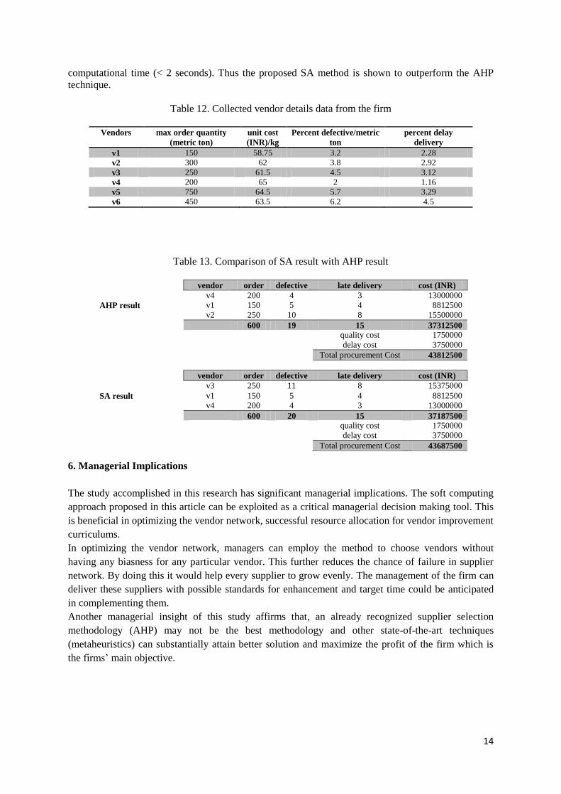
Table 13. Comparison of SA result with AHP result

6. Managerial Implications

The study accomplished in this research has significant managerial implications. The soft computing

approach proposed in this article can be exploited as a critical managerial decision making tool. This

is beneficial in optimizing the vendor network, successful resource allocation for vendor improvement

curriculums.

In optimizing the vendor network, managers can employ the method to choose vendors without

having any biasness for any particular vendor. This further reduces the chance of failure in supplier

network. By doing this it would help every supplier to grow evenly. The management of the firm can

deliver these suppliers with possible standards for enhancement and target time could be anticipated

in complementing them.

Another managerial insight of this study affirms that, an already recognized supplier selection

methodology (AHP) may not be the best methodology and other state-of-the-art techniques

(metaheuristics) can substantially attain better solution and maximize the profit of the firm which is

the firms’ main objective.

vendor order defective late delivery cost (INR)

v4 200 4 3 13000000

AHP result v1 150 5 4 8812500

v2 250 10 8 15500000

600 19 15 37312500

quality cost 1750000

delay cost 3750000

Total procurement Cost 43812500

vendor order defective late delivery cost (INR)

v3 250 11 8 15375000

SA result v1 150 5 4 8812500

v4 200 4 3 13000000

600 20 15 37187500

quality cost 1750000

delay cost 3750000

Total procurement Cost 43687500

15

7. Conclusions

This article portrays a novel SA based metaheuristic algorithm to select the supplier for a particular

Indian firm which is an NP-complete problem in nature. The problem is formulated using

multiobjective mathematical model which reflects the essential optimization criteria of this research.

The initial feasible solution to the proposed SA based technique is obtained using AHP technique in

order to quicken the computation. This work further exploits Taguchi’s robust design approach to

select optimal set of parameters to SA algorithm which is crucial in influencing the performance of

the technique. The uniqueness of this work lies in practicing two different decision making techniques

in solving this MCDM problem model. In past literature such metaheuristic approach to evaluate and

enhance the AHP ranking of vendors has never been carried out. To perform the said analysis authors

have collected industrial data from a national construction firm. Computational results presented in

Section 5 demonstrate that the SA method outperforms the AHP technique performing better than the

AHP method for the supplier selection problem. The proposed SA procedure produces nearly 0.3%

improved solution. This work is an experimental study which considered the main criteria of the

problem such as cost, delivery and delay. However many other intricate sub-criteria could also be

considered to make this work more realistic. Future work can be accomplished by utilizing this

technique in more complex supplier selection problems incorporating more conflicting criteria and

sub-criteria by considering risk factors or suppliers profiles and other related issues and that is the

possible extension of this research.

Acknowledgement

The authors are grateful to the anonymous reviewers for their valuable comments and suggestions in

improving the quality of the paper.

References

Aarts, E., and Korst, J. (1990) Simulated Annealing and the Boltzmann Machine, John Wiley & Sons,

New York, USA.

Aissaoui, N., Haouari, M., and Hassini, E. (2007) ‘Supplier selection and order lot sizing modeling: A

review’, Computers & Operations Research, Vol. 34, No. 12, pp. 3516-3540.

Akarte, M.M. (2001) ‘Web based casting supplier evaluation using analytic hierarchy process’,

Journal of the Operational Research Society, Vol. 52, No. 5, pp. 511-522.

Amid, A. Ghodsypour, S.H., and O’Brien, C. (2009) ‘A weighted additive fuzzy multiobjective model

for the supplier selection problem under price breaks in a supply Chain’, International Journal of

Production Economics, Vol. 121, No. 2, pp. 323-332.

Amid, A. Ghodsypour, S.H., and O’Brien, C. (2010) ‘A weighted max–min model for fuzzy multi-

objective supplier selection in a supply chain’, International Journal of Production Economics,

doi:10.1016/j.ijpe.2010.04.044 (article in press).

Arunkumar, N., Karunamoorthy, L., and Makeshwaraa, N.U. (2007) An optimization technique for

vendor selection with quantity discounts using genetic algorithm’, Journal of Industrial

Engineering International, Vol. 3, No. 4, pp. 1-13.

Bello, M.J.S. (2003) A case study approach to the supplier selection process, M.Sc. thesis, submitted

to University of the Puerto Rico Mayaguez.

Zhao, G., and Bross, M.E. (2004) Supplier selection process in emerging markets - The Case Study of

Volvo Bus Corporation in China, M.Sc. thesis, submitted to Göteborg University, Sweden.

Chen, C.T., Lin, C.T., and Huang, S.F. (2006) ‘A fuzzy approach for supplier evaluation and selection

in supply chain management’, International Journal of Production Economics, Vol. 102, No. 2,

pp. 289–301.

16

Choy, K.L., Lee, W.B., and Lo, V. (2002) ‘An intelligent supplier management tool for benchmarking

suppliers in outsource manufacturing’, Expert Systems with Applications, Vol. 22, No, 3, pp. 213-

224.

Dickson, G.W. (1966) ‘An Analysis of Vendor Selection: Systems and Decisions’, Journal of

Purchasing, Vol. 1, No. 2, pp. 5-17.

Ding, H., Benyoucef, L., and Xie, X. (2003) ‘A simulation-optimization approach using genetic

search for supplier selection’, Proceedings of the 2003 Winter Simulation Conference, pp. 1260-

1267.

Ellram, L.M. (1990) ‘The Supplier Selection Decision in Strategic Partnerships’, Journal of

Purchasing and Materials Management, Vol. 26, No. 4, pp. 8-14.

Gnanasekaran, S., Velappan S., and Manimaran, P. (2010) ‘An integrated model for supplier selection

using fuzzy analytical hierarchy process: a steel plant case study’, International Journal of

Procurement Management, Vol. 3, No. 3, pp. 292-315.

Handfield, R., Walton, S.V., and Sroufe, R. (2002) ‘Applying environmental criteria to supplier

assessment: A study in the application of the Analytical Hierarchy Process’, European Journal of

Operational Research, Vol. 141, No. 1, pp. 70-87.

Kanagaraj, G., and Jawahar, N. (2009) ‘A simulated annealing algorithm for optimal supplier

selection using the reliability-based total cost of ownership model’, International Journal of

Procurement Management, Vol. 2, No. 3, pp. 244-266.

Kubat, C., and Yuce, B. (2006) ‘Supplier Selection with Genetic Algorithm and Fuzzy AHP’,

Proceedings of 5th International Symposium on Intelligent Manufacturing Systems, pp. 1382-

1401.

Lee, A.H.I, Chen, W.C., and Chang, C. J. (2008) ‘A fuzzy AHP and BSC approach for evaluating

performance of IT department in the manufacturing industry in Taiwan’, Expert Systems with

Applications, Vol. 34, No. 1, pp. 96-107.

Li, C.C., Fun, Y.P., and Hung, J.S. (1997) ‘A new measure for supplier performance evaluation’, IIE

Transactions, Vol. 29, No. 9, pp. 753-758.

Liu, F.H.F., and Hai, H.L. (2005) ‘The voting analytic hierarchy process method for selecting

supplier’, International Journal of Production Economics, Vol. 97, No. 3, pp. 308-317.

Ng, W.L. (2008) ‘An efficient and simple model for multiple criteria supplier selection problem’,

European Journal of Operational Research, Vol. 186, No. 3, pp. 1059–1067.

Petroni, A., and Braglia, M. (2000) ‘Vendor selection using principal component analysis’, Journal of

Supply Chain Management, Vol. 36, No. 2, pp. 63-69.

Rajkumar, C.J., Kannan, S.M., Jayabalan, V. (2009) ‘Multicriteria-based customer-focused vendor

selection through the analytic hierarchy process’, International Journal of Procurement

Management, Vol. 2, No. 2, pp. 143-162.

Rezaei, J., and Davoodi, M. (2008) ‘A deterministic, multi-item inventory model with supplier

selection and imperfect quality’, Applied Mathematical Modelling, Vol. 32, No. 10, pp. 2106–

2116.

Saaty, T.L. (1980) The Analytic Hierarchy Process: Planning, Priority Setting, Resource Allocation.

New York: McGraw-Hill.

Saen, R.F. (2008) ‘Using super-efficiency analysis for ranking suppliers in the presence of volume

discount offers’, International Journal of Physical Distribution & Logistics Management, Vol. 38,

No. 8, pp. 637-651.

Saen, R.F., and Zohrehbandian, M. (2008) ‘A data envelopment analysis approach to supplier

selection in volume discount environments’, International Journal of Procurement Management,

Vol. 1, No. 4, pp. 472-488.

Saen, R.F. (2009) ‘Using data envelopment analysis for ranking suppliers in the presence of

nondiscretionary factors’, International Journal of Procurement Management, Vol. 2, No. 3, pp.

229-243.

Saen, R.F. (2010) ‘Restricting weights in supplier selection decisions in the presence of dual-role

factors’, Applied Mathematical Modelling, Vol. 34, No. 10, pp. 2820–2830.

Schooner, S. (2003) ‘Commercial Purchasing: The Chasm between the United State Government’s

Evolving Policy and Practice’, In: Arrowsmith, S., and Trybus, M. (Eds.), Public Procurement:

The Continuing Revolution, (pp. 137-169), Kluwer Law International, The Hague.

17

Scott, S. (1995) ‘Best Value Contracts: Lessons Learned in Paving the Road to Quality’, National

Contract Management Journal, Vol. 26, No. 2, pp. 1-11.

Taguchi, G. (1994) ‘Taguchi on Robust Technology Development: Bringing Quality Engineering

Upstream’, Journal of Electronic Packaging, Vol. 116, No. 2, pp. 161.

Tahriri, F., Osman, M.R., Ali, A., and Yusuff, R.M. (2008) ‘A Review of Supplier Selection Methods

in Manufacturing Industries’, Suranaree Journal of Science and Technology, Vol. 15, No. 3, pp.

201-208.

Tam, M.C.Y, and Tummala, V.M.R. (2001) ‘An application of the AHP in vendor selection of a

telecommunications system’, Omega, Vol. 29, No. 2, pp. 171-182.

Thompson K.N. (1990) ‘Vendor Profile Analysis’, Journal of Purchasing and Materials

Management, Vol. 26, No. 1, pp. 11-18.

Timmerman, M. (1986) ‘An approach to vendor performance evaluation’, Engineering Management

Review, IEEE, Vol. 15, No. 3, pp. 14-20.

Weber C., Current, J.R., and Benton, W.C. (1991) ‘Vendor Selection Criteria and Methods’,

European Journal of Operational Research, Vol. 50, No. 1, pp. 2-18.

Wu, D. (2009) ‘Supplier selection: A hybrid model using DEA, decision tree and neural network’,

Expert Systems with Applications, Vol. 36, No. 5, pp. 9105–9112.

Yahya, S., and Kingsman, B. (1999) ‘Vendor rating for an entrepreneur development programme: a

case study using the analytic hierarchy process method’, Journal of the Operational Research

Society, Vol. 50, No. 5, pp. 916-930.

Yu, X., and Jing. S. (2004) ‘A Decision Model for Supplier Selection Considering Trust’, Chinese

Business Review, Vol. 3, No. 6, pp. 15-20.