An Architecture for Task Execution in Adverse Environments
223
An Architecture for Task Execution in Adverse Environments Filip MILETI ´ C
-
Upload
khangminh22 -
Category
Documents
-
view
4 -
download
0
Transcript of An Architecture for Task Execution in Adverse Environments

An Architecture for Task Execution in
Adverse Environments
Filip MILETIC


An Architecture for Task Execution in
Adverse Environments
Proefschrift
ter verkrijging van de graad van doctoraan de Technische Universiteit Delft,
op gezag van de Rector Magnificus prof. dr. ir. J. T. Fokkema,voorzitter van het College voor Promoties,
in het openbaar te verdedigen op maandag 4 juni 2007 om 12.30 uur,
door Filip MILETIC
Electrical Engineer van de Universiteit van Belgrado, Serviegeboren te Krusevac, Servie.

Dit proefschrift is goedgekeurd door de promotor:
Prof. dr. ir. P. M. Dewilde
Samenstelling promotiecommissie:Rector Magnificus voorzitterProf. dr. ir. P. M. Dewilde Technische Universiteit Delft, promotorProf. dr. M. Prokin Universiteit van BelgradoProf. dr. ir. A. J. van der Veen Technische Universiteit DelftProf. dr. ir. F. C. A. Groen Universiteit van AmsterdamProf. dr. ir. I. G. M. M. Niemegeers Technische Universiteit Delftdr. drs. L. J. M. Rothkrantz Technische Universiteit Delftdr. K. Nieuwenhuis DECISProf. dr. K. G. W. Goossens Technische Universiteit Delft, reservelid
Copyright c© 2007 by Filip Miletic
All rights reserved. No part of the material protected by this copyright noticemay be reproduced or utilized in any form or by any means, electronic ormechanical, including photocopying, recording or by any information storageand retrieval system, without the prior permission of the author.
ISBN: 978-90-9021920-2

To Milan


Contents
1 Introduction 11.1 Outline of This Chapter . . . . . . . . . . . . . . . . . . . . . . . . 21.2 Background . . . . . . . . . . . . . . . . . . . . . . . . . . . . . . . 21.3 Properties . . . . . . . . . . . . . . . . . . . . . . . . . . . . . . . . 81.4 Problem Statement . . . . . . . . . . . . . . . . . . . . . . . . . . . 111.5 Contributions . . . . . . . . . . . . . . . . . . . . . . . . . . . . . . 121.6 Outline of The Thesis . . . . . . . . . . . . . . . . . . . . . . . . . 14
2 Toolkit 172.1 Introduction . . . . . . . . . . . . . . . . . . . . . . . . . . . . . . . 172.2 Description Quality Requirements . . . . . . . . . . . . . . . . . . 182.3 Representation with Object-Z and CPN . . . . . . . . . . . . . . . 192.4 Object-Z Description . . . . . . . . . . . . . . . . . . . . . . . . . . 202.5 The Petri Net (PN) and Coloured Petri Net (CPN) Descriptions . 242.6 CPN Simulation by a Blackboard . . . . . . . . . . . . . . . . . . . 322.7 Blackboard Semantics . . . . . . . . . . . . . . . . . . . . . . . . . 342.8 CPN Simulation with a Blackboard . . . . . . . . . . . . . . . . . . 372.9 Summary . . . . . . . . . . . . . . . . . . . . . . . . . . . . . . . . 48
3 Architecture Overview 493.1 Introduction . . . . . . . . . . . . . . . . . . . . . . . . . . . . . . . 493.2 Resources . . . . . . . . . . . . . . . . . . . . . . . . . . . . . . . . 523.3 Layering . . . . . . . . . . . . . . . . . . . . . . . . . . . . . . . . . 533.4 Componentized Layer Structure . . . . . . . . . . . . . . . . . . . . 553.5 Component Overview . . . . . . . . . . . . . . . . . . . . . . . . . 563.6 Summary . . . . . . . . . . . . . . . . . . . . . . . . . . . . . . . . 61
4 Task Mapping 634.1 Introduction . . . . . . . . . . . . . . . . . . . . . . . . . . . . . . . 634.2 Requirements . . . . . . . . . . . . . . . . . . . . . . . . . . . . . . 644.3 Enabler Mapping (EM) . . . . . . . . . . . . . . . . . . . . . . . . 684.4 Mapping Tasks to Nodes . . . . . . . . . . . . . . . . . . . . . . . . 724.5 Distributed Blackboard . . . . . . . . . . . . . . . . . . . . . . . . 77
vii

viii CONTENTS
4.6 Related Work . . . . . . . . . . . . . . . . . . . . . . . . . . . . . . 804.7 Summary . . . . . . . . . . . . . . . . . . . . . . . . . . . . . . . . 82
5 The Environment and Storage Model 855.1 Introduction . . . . . . . . . . . . . . . . . . . . . . . . . . . . . . . 855.2 Connectivity Function . . . . . . . . . . . . . . . . . . . . . . . . . 905.3 The Storage Model . . . . . . . . . . . . . . . . . . . . . . . . . . . 965.4 System Model . . . . . . . . . . . . . . . . . . . . . . . . . . . . . . 985.5 Summary . . . . . . . . . . . . . . . . . . . . . . . . . . . . . . . . 106
6 Core Based Tree (CBT) 1096.1 Introduction . . . . . . . . . . . . . . . . . . . . . . . . . . . . . . . 1096.2 Problem Description . . . . . . . . . . . . . . . . . . . . . . . . . . 1156.3 Solution Outline . . . . . . . . . . . . . . . . . . . . . . . . . . . . 1186.4 Algorithm Description . . . . . . . . . . . . . . . . . . . . . . . . . 1246.5 Performance . . . . . . . . . . . . . . . . . . . . . . . . . . . . . . . 1386.6 Summary . . . . . . . . . . . . . . . . . . . . . . . . . . . . . . . . 140
7 The Execution Model 1457.1 Introduction . . . . . . . . . . . . . . . . . . . . . . . . . . . . . . . 1457.2 Data Model . . . . . . . . . . . . . . . . . . . . . . . . . . . . . . . 1467.3 Matching . . . . . . . . . . . . . . . . . . . . . . . . . . . . . . . . 1637.4 The Workflow Mechanics . . . . . . . . . . . . . . . . . . . . . . . 1797.5 Summary . . . . . . . . . . . . . . . . . . . . . . . . . . . . . . . . 195
8 Conclusion 1978.1 Introduction . . . . . . . . . . . . . . . . . . . . . . . . . . . . . . . 1978.2 Why Distributed Workflow Execution Now . . . . . . . . . . . . . 1988.3 Future Work . . . . . . . . . . . . . . . . . . . . . . . . . . . . . . 199
Bibliography 201
Acknowledgments 209
Samenvatting 211
About the Author 213

Chapter 1
Introduction
This thesis describes an architecture for distributed computation in mobile envi-ronments. Here, the workflow stands for the operational aspect of a work proce-dure. This notion subsumes the structure of the tasks, who performs them, whattheir operation structure is, how they are synchronized, how information flows tosupport the tasks and how they are tracked. The designed architecture is testedin a proof-of-concept implementation named Distributed Workflow Execution Ar-chitecture for Mobile (DWEAM).
The interest in distributed workflow [90] execution architectures is long stand-ing (some examples thereof are given further in the text). However, there has notyet been an adequate treatment of workflow execution in mobile systems. Thebenefits of such a system would be collected by users who perform a coordinatedtask in a complex environment and must establish own coordination infrastructureto do so. Typical users are the members of emergency rescue teams, i.e. police,fire brigade or medical personnel, when handling an incident, where the cooper-ation between the team members is hindered by mobility and adverse communi-cation conditions. The communication via the Global System for Mobile (GSM)networks, that are used in small scale operations in urban areas cannot offer ap-propriate quality of service in face of escalation or infrastructure damage. Thenow-aged broadcast radio (i.e. walkie-talkie) typically does not support the cou-pling with information systems, as it is intended for the communication betweenhumans. We therefore consider a system architecture that addresses the commu-nication issues, while being infrastructure-independent and supporting both thework procedures for human operators, as well as that of the information systems.
In Europe, the market penetration percentage for GSM devices has long sur-passed 80%, and tending to 100% [6], and the market drive thus created motivatesthe producers to equip their products with ever more computing power. This re-sulted in the advent of Personal Digital Assistants (PDA) and the convergenceof the two technologies in the near future seems imminent. Assuming that inthe near future mobile computing devices with communication facilities would be
1

2 CHAPTER 1. INTRODUCTION
routinely used, we recognize the potential for improving cooperative work thatthese devices offer. We consider this enough motivation to investigate and designa system that takes advantage of such devices. The example use case involvingassistance to emergency services is just one of many possible future uses.
1.1 Outline of This Chapter
This introductory chapter begins the thesis by introducing the background of theproblem in Section 1.2. The Section 1.4 states the research problem. Following abrief discussion of the preliminaries, we formulate the research question, and giveits decomposition to three sub-problems. The suggested solutions to the researchsub-problems are stated thereafter, as well as the improvements to the state ofthe art as given by this thesis. Finally, the Section 1.6 describes in brief the otherchapters in this thesis.
1.2 Background
Distributed computing subsumes the topic of concurrent execution of algorithmson a collection of computing resources (processors, computers, nodes). We will beconsidering distributed computer systems in detail, so abbreviations “computersystem” and “system” will always stand for such distributed systems.
Distributed computing was initially intended for large computation tasks as-sociated with research in natural sciences, mathematics and like areas. Since theadvent of the world-wide Internet, forms of distributed computing have becomeparts of daily lives. Trade, commerce, banking, mailing, along with a line ofother ages old activities, were adorned with the prefix “e-” to reflect their new al-liance with the information technology. The Internet has thus brought distributedcomputing to the desktop. The wide spread use of computers and the global in-terconnection such as the Internet gave a natural motivation to harness the largecollective computing power. Example projects are Distributed Net (brute forcecode breaking, see [2]), Seti@Home (a search for artificial signals coming fromdeep space [74]), and Folding@Home (protein folding [31]). The University ofCalifornia at Berkeley maintains BOINC [13], a framework to support this kindof “bona-fide collective” distributed computing. These examples show how com-puters worldwide can be joined together to perform a large task.
A promising new field for distributed computing is formed with the adventof mobile computers. GSM phones and PDAs have entered the scene during thenineties, likely to be followed by other smart wearable devices. They populatedthe earth in even greater numbers than personal computers, and it is expectedthat the growth would continue in the upcoming years. Apart from their ini-tial applications, these devices are usually fully capable machines, every moreoften able to communicate with like machines in their vicinity. It can be inferredthat these machines, when properly joined together, could perform significant

1.2. BACKGROUND 3
computational tasks for the collective of their owners and offer a range of newapplications. For this vision to become a reality, a host of issues must be resolvedso that effective computation becomes possible.
An informal notion of an effective computation is that which takes on a suit-ably posed question and produces an answer obtained by a sequence of well-definedprimitive steps (i.e. an algorithm) to yield an answer with some predefined qual-ity properties; additionally, presentation qualities may be involved, as specified bythe Human-Computer Interface (HCI) guidelines. The quality properties definethe manner in which the computer system produces an answer: how much timeit takes whether it is of a good enough quality etc. As Gartner [33] reported, in1977 Lamport [48] observed that the system properties can be be put into twodistinct classes: safety properties and liveness properties. The safety propertiesstate that “something bad never happens”, i.e. that under no condition the sys-tem is to enter an unwanted state. The liveness properties state that “eventuallysomething good happens”, i.e. that the system eventually reaches some statewith favorable properties (e.g. a state in which the computational outcome is pre-sented). Effectiveness is therefore restated in terms of both liveness and safety, aswell as subjective measurement of the usefulness of the system, as perceived bythe users. By liveness, an effective system must present the user with an answer(if the result can be computed given the system’s capabilities). By safety, theresult must be correct, supplied within a given time frame, incurring a limitedresource cost, possibly others. By HCI requirements the system must facilitateHCI by timely presentation, detail abstraction and ease of use.
A computer system’s effectiveness fundamentally depends on its architecture.It is thus important to have at hand a categorization of distributed architectures.Being able to classify our system informs us of its possibilities. A choice of the ar-chitecture will determine the set of computational tasks that the computer systemcan and can not perform. Allowing the possibility of faults in the computationfurther segregates the possible from the impossible. According to Lynch ([51],Chapter 1), the distributed algorithms can differ by a number of attributes ulti-mately determined by the architectural choices:
1. The communication method. This concerns distributed algorithms run-ning on a collection of processors that must communicate somehow. Com-mon methods of communication include addressing shared memory, sendingpoint-to-point or broadcast messages and executing remote procedure calls.The ordering of messages can be important too.
2. The timing model. This concerns the manner in which different processorsexecute their separate tasks. At one extreme, the processors run in lock-step, progressing in perfect synchrony. At the other extreme, they can eachrun at various relative speeds and can take arbitrary execution turns. Inbetween the extremes are various partially synchronous systems, in whichthe processors have partial information about timing.

4 CHAPTER 1. INTRODUCTION
3. The failure model. This concerns the way that the hardware may fail toperform its tasks. It can be assumed to be completely reliable, yielding afault-free assumption. Or it may be required to tolerate some fraction offailures.
4. The addressed problems. This concerns the problems that one attempts tosolve by a distributed system. Typical problems of this sort are resourceallocation, concurrency control, deadlock detection, global snapshots, syn-chronization and implementation of various types of objects.
The properties are implied by the adopted use case. The communicationmethod employed in our approach (and the DWEAM system) is localized point-to-point as the nodes are assumed to communicate only with other geographicallyclose nodes. The timing model is virtually synchronous as the nodes run inde-pendently except for few points where message exchange takes place. The failuremodel we consider is communication and node fail-stop, as the nodes and their in-terconnections can fail (and recover) at runtime. Finally the addressed problemsconcern the efficiency of the computation in such an environment.
A World of (Im)possibilities
The effects of system attributes with respect to the classification given by Lynchwere succinctly commented in a paper by Turek and Shasha [43], by analyzing afictitious storyline named “The Parable of La Tryste”. They comment the solutionof the prototypical consensus problem that arises in distributed computing. Theyexplain when consensus problem is solvable, when it is not, and when unsolvable,how the problem can be relaxed so that a solution can be found.
“Bob and Alice have discovered that they have a lot in common. Forexample, they both prefer e-mail to telephone. On a cold winter day,Alice sends Bob electronic mail at 10a.m. saying ‘Let’s meet at noonin front of La Tryste.’ ”
“The e-mail connection between our two protagonists is known to losemessages, but today they are lucky and Alice’s message arrives atBob’s workstation at 10:20a.m. Bob looks at his calendar and sees heis free for lunch. So he sends an acknowledgment.”
“Alice receives the acknowledgment at 10:45a.m. and prepares to goout, when a thought occurs to her: ‘If Bob doesn’t know that I receivedhis acknowledgment, he might think I won’t wait for him. I’d betteracknowledge his acknowledgment.’ ”
“And so it goes. We can show that, ultimately, neither Bob nor Alicewill make it to La Tryste unless at least one of them is willing to riskwaiting in the cold without meeting the other.”

1.2. BACKGROUND 5
The “La Tryste” scenario demonstrates the difficulty of reaching a consensus insystems with asynchronous operation, unbounded message delays, and possiblemessage loss. The problem is that as sending the message can fail, neither Bobnor Alice can know whether their decision is communicated to the other. In fact,under these conditions, Lynch et al. have proved that consensus is impossible [52].
This result brings us to an apparent conflict with what we perceive in daily life.Despite the impossibility of communication, people and computers do manage tocooperate and things do get done. The apparent conflict comes from the waythe problem is analyzed. Given that no errors in communication are allowed,and the fact that no matter how many times the message exchange is repeated,we are never able to rule out the worst case (as all communication eventuallyends in an error), regardless of how improbable it might be. A conclusion followsthat the problem as posed has no solution. Thus the requirement on reliablecommunication must be relaxed for the result to be applicable in the real world.The outline of this approach is given in the following Section.
The Information Theoretic Approach
Now turn to the area of information theory, where a similar problem has long beensolved by Shannon [75] (numerous others followed) who formulated the commu-nication problem and gave a set of initial solutions. A Message chosen from apredetermined fixed alphabet is transferred from an Information Source to a Des-tination (see Figure 1.1). Before sending, the Message is encoded for transmission
SM // T
S //RS // R
M // D
N
OO
Figure 1.1: The communication system setup, as given by Shannon [75]. S: Source.T: Transmitter. R: Receiver, N: Noise, D: Destination. M: Message , S: Signal,RS: Received Signal.
by a Transmitter where it becomes a Signal. The Signal is sent through a com-munication channel, where it is inevitably affected by noise (its effect modeledby a Noise Source). The Receiver obtains a likely distorted Received Signal, anddecodes it so as to obtain a Message which is finally forwarded to the destination.
The difference with the “La Tryste” is that the probabilities of communicationfailure are taken into account. Shannon’s conclusion from here is that providedthe communication channel is used the right way, the communication could be

6 CHAPTER 1. INTRODUCTION
made as reliable as needed. However, the price one pays for this is that in principlemore information needs to be sent over the channel than is minimally required todescribe the message.
Example 1 (Binary Symmetric Channel) Let us temporarily diverge fromthe original “La Tryste” and consider the example of a binary symmetric channel,as given in Figure 1.2. In this example, the communication channel is binary, i.e.
•01−p //
p
???
????
????
?? • 0
•11−p
//p
?? • 1
Figure 1.2: The binary symmetric channel model, with error probability p perchannel use.
two distinct messages can be sent, and only one of the two can be sent at a time.Call these “1” and “0”, or in the case of “La Tryste”, call them “yes, let’s meet”,and “sorry, I’m busy”. When the Information Source can produce more than twodistinct messages, they can be sent by using the binary channel several times, sothat different sequences consisting of zeros and ones denote different messages.The total of ⌈log2 M ⌉ channel uses are needed so that there are at least M dis-tinct binary sequences. This is a familiar scenario frequently occurring in digitalcommunications, including that between computer systems.
Due to noise, each channel use can be distorted, so that a “1” that has beensent becomes a “0” or vice-versa. This happens with some probability p. Thusthe probability is 1 − p that one channel use ends with no errors. This paral-lels the possibility that a “yes” might be flipped to “no” in transit, or other wayaround. Shannon determined that there is a fundamental limit for the rate (inbits per channel use) at which one can transmit information through this (or forthat matter, any other) channel, which he called the capacity. For the binarysymmetric channel it is given by [21]:
C = H (p) = −p log2 p − (1− p) log2(1 − p).
In this expression, H (p) is the entropy of a binary source. Moreover, it wasdetermined that transmitting through such a channel cannot be done at a ratehigher than C . The capacity of a binary channel with respect to the probability pis given in Figure 1.3.
What use is this for Alice and Bob? First one sees that in most of the cases(except at the endpoints of the graph in Figure 1.3 corresponding to p = 0 andp = 1), they cannot expect to transfer a whole message (i.e. “fully” agree whether

1.2. BACKGROUND 7
0 0.1 0.2 0.3 0.4 0.5 0.6 0.7 0.8 0.9 10
0.1
0.2
0.3
0.4
0.5
0.6
0.7
0.8
0.9
1
Probability of error per channel use
Channel
capaci
ty
Capacity of the Binary Symmetric Channel
Figure 1.3: The capacity of the binary symmetric channel in bits per channel use,versus the probability p of error per channel use.
a meeting goes through or not) by just a single channel use. By multiple channeluse they could repeat the agreement over and over and then take a majority vote.But then, their information rate (i.e. say the price they pay for the communicationper unit transferred messages) will increase with the number of repetitions, whichis also not good.
However, if Alice and Bob agree to set not one, but several meetings at once,it would be possible to agree on C ·m independent meetings by exchanging onlym messages (and therefore paying the amount proportional to m for the con-versation), and do this with as small probability of error as desired. In reality,driving the error probability close to zero would also mean having to agree on animpossibly long sequence of meetings at once, but this realistic complication isnot considered important in the model.
Example 2 (Binary Erasure Channel) Consider now a setup that is some-what different and closer to “La Tryste”. The new channel is shown in Figure 1.4.

8 CHAPTER 1. INTRODUCTION
For each sent binary symbol, there is a probability p that it gets lost in the chan-
•01−p //
p
???
????
?? • 0
• ε
•01−p
//
p
?? • 1
Figure 1.4: The binary erasure channel [75].
nel. The loss is denoted at the Receiver by a third symbol ε. Otherwise, with theprobability 1− p the symbol is received unchanged.
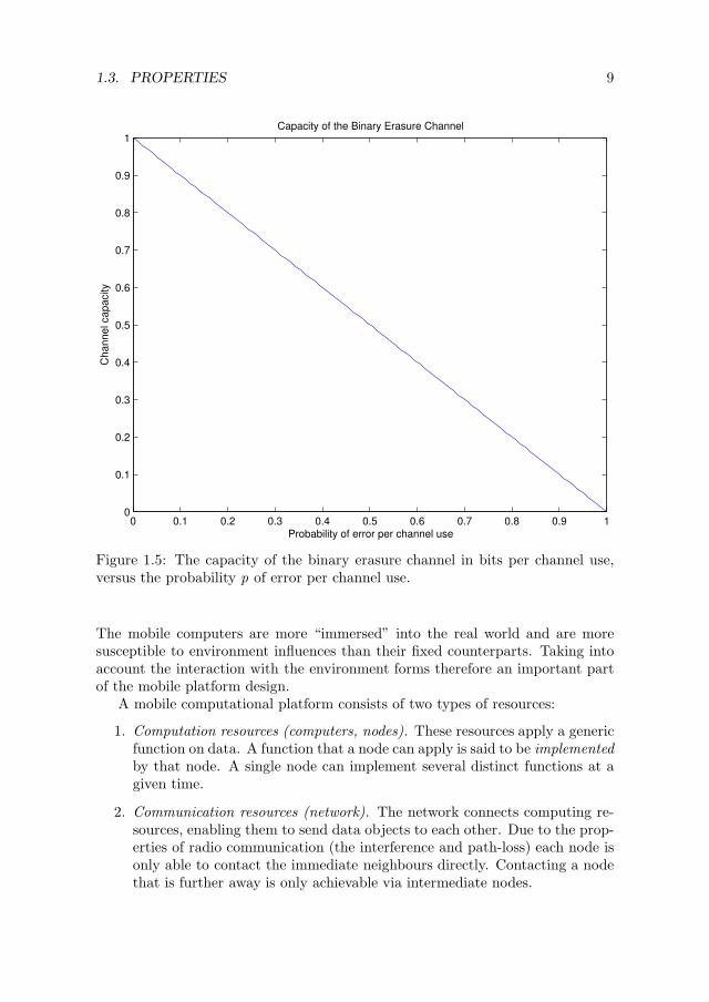
This channel model is better for computer networks than the binary symmetricchannel. The computer networks are commonly packet-switched, with messages ofvarious origins being multiplexed and sent through the same channel, only for thisprocess to be reversed at the other end. The packet-switches operate by stackingall the transmissions pending delivery in an outbound queue, which is emptied aspackets are being sent. As queues have limited capacity, it is possible that a packetarriving at a switch with a full transmit queue will get dropped. Such omissionsare be perceived as erasures at the receiver. In this case, the channel capacity isgiven by a simpler expression:
C = 1− p,
which is at the same time the expected fraction of lossless transmissions.
The contrast of “La Tryste” and the communication examples 1 and 2 showsimportant differences in approach. The impossibility result illustrated in the for-mer employs a pessimistic analysis, whereby only the worst case is considered.On the other hand, the communication example takes into account a more re-alistic scenario and an advanced approach yielding provably better performance,at the cost of an (arbitrarily small) probability of error. One can note the useof the statistical properties of the communication channel to yield the desiredperformance.
The statistical properties of the environment will come back at several pointsin the analyses given in the upcoming chapters.
1.3 Properties
The Resources
Building a computation platform out of mobile devices connected by wirelessnetwork somewhat from the design of conventional (fixed) computer networks.
1.3. PROPERTIES 9
0 0.1 0.2 0.3 0.4 0.5 0.6 0.7 0.8 0.9 10
0.1
0.2
0.3
0.4
0.5
0.6
0.7
0.8
0.9
1Capacity of the Binary Erasure Channel
Probability of error per channel use
Channel capacity
Figure 1.5: The capacity of the binary erasure channel in bits per channel use,versus the probability p of error per channel use.
The mobile computers are more “immersed” into the real world and are moresusceptible to environment influences than their fixed counterparts. Taking intoaccount the interaction with the environment forms therefore an important partof the mobile platform design.
A mobile computational platform consists of two types of resources:
1. Computation resources (computers, nodes). These resources apply a genericfunction on data. A function that a node can apply is said to be implementedby that node. A single node can implement several distinct functions at agiven time.
2. Communication resources (network). The network connects computing re-sources, enabling them to send data objects to each other. Due to the prop-erties of radio communication (the interference and path-loss) each node isonly able to contact the immediate neighbours directly. Contacting a nodethat is further away is only achievable via intermediate nodes.

10 CHAPTER 1. INTRODUCTION
The special properties of the mobile computing platform, constituting thedesign constraints, are:
1. Node volatility. Mobile nodes are power-constrained. Thus they can runout of power and forcibly become unreachable. The nodes can also bedestroyed. This constitutes a involuntary leave. Nodes can also be shutdown, constituting a voluntary leave.
2. Network volatility. Due to path-loss and interference in the radio-based net-work, and the fact that the nodes change position over time, each individuallink between pairs of nodes is subject to variation.
The Tasks
The mobile platform is assembled so that some predefined computational taskcan be performed. Interesting tasks for distributed execution are such that canbe decomposed into loosely coupled subtasks. Thus, the patterns of cooperationbetween nodes are not random. Rather, they follow a specific pattern, as deter-mined by the task dependency. Furthermore, an allocation schema must existwhereby tasks are allocated for execution (i.e. mapped) to nodes.
Thus the task execution is characterized by the following properties:
1. Static structure. This concerns the way the tasks relate to each other, i.e.how they are subordinated what their mutual dependencies are, and whichoperations on the data they perform.
2. Dynamic structure. This concerns the rules by which the tasks are executed,and the management of the data flow between dependent tasks.
3. Mapping to nodes. This concerns allocating tasks to nodes and handlingthe volatility.
These properties taken together constitute a workflow.
The Users
An important design goal for DWEAM is the easy integration of the users inputin the overall system works. The user experience is not treated, as it is consideredan HCI issue out of scope of this thesis. However, providing an uniform interfacefor the coupling of the machine generated and user-supplied result is important.To distinguish between these two classes of system participants we use the termagent, when a machine participant in the system is meant and actor for a humanparticipant in the system. Together they are all named workers.

1.4. PROBLEM STATEMENT 11
1.4 Problem Statement
We consider, in essence, a distributed computing system intended to execute aspecified abstract computing task, under resource volatility. We represent thecomputing task by a workflow. The workers are capable of executing a subset oftasks in a workflow.
1. Execution speed. Multiple tasks are executed in parallel. This can not onlybe faster when compared to sequential processing for well-structured tasks,but can also scale with the number of available workers.
2. Separation of concern. It is possible to map special processes to workerswith special capabilities. A failed agent can be replaced with one havingcomparable capabilities. A task intended for an absent actor can be re-assigned.
3. Mixed initiative system support. It is possible to mix the active participationof the agents and actors in task execution.
Research Question
The thesis is the answer to a single research question: How is computation struc-tured and controlled in this environment?
The research question decomposes into interwoven sub-problems:
1. The Environment Model. An environment model is needed to express theenvironment influence to DWEAM performance.
What is an appropriate model for the environment of this distributed system?What are its properties and what design patterns can be derived from it?
2. The Storage Model. The storage resources accessible to the entire systemvary over time. Thus in addition to conventional data storage mechanisms,special care must be taken to ensure storage availability despite the timevariations.
What does this mechanism look like? What is its performance?
3. The Execution Model. The computational resources offered to the entiresystem vary over time. Thus in addition to conventional execution mech-anisms, special care must be taken to ensure the computational resourceavailability despite time variations.
What does this mechanism look like? What is its performance?

12 CHAPTER 1. INTRODUCTION
1.5 Contributions
The solution components answer in turn each of the three research sub-problems.They form the core contributions of this thesis.
1. The Erasure Graph answers the Environment Model question. It capturesthe properties of the environment the system nodes are embedded in. Theanalysis of the Erasure Graph yields performance bounds for both the Stor-age and Execution model.
2. The Distributed Coding answers the Storage Model question. In view of theErasure Graph model, a technique is devised for resource-efficient and fault-tolerant data distribution. In this technique, we consider the serializationof data into binary streams, and the distribution of parts of these streamsto independent nodes. We give the estimate of the storage capacity for themodel thus obtained.
3. The Event Notification answers the Execution Model question. In view ofthe Erasure Graph model, a technique is devised for dynamic workflow as-sembly, maintenance and execution. The event notification is based on theCore Based Tree (CBT), a tree-like structure that ensures all the requiredconnections can be established. The performance of the CBT is estimatedThe connections are established using content-based addressing whereby forcommunication, the contents of the messages are used to route them to allthe intended recipients. Finally, the execution model is formulated thatguarantees the execution of the CPN implemented by the nodes participat-ing in the event notification structure.
The solution components are being implemented into DWEAM, the proof-of-concept system.
Advances with Respect to the State of the Art
The contributions to the state of the art, made in this thesis, are as follows.
1. The formulation of distributed computation in volatile environments as adistributed execution of a CPN, and its description in terms of the Object-Z language (see Chapter 2). This contribution enabled us to identify thattoken preservation and object delivery were needed to ensure the distributedworkflow execution.
2. The formalism casting the informally described tasks with the foremost aimto enable the formalization of tasks performed by the emergency rescueteams from the context of Chaotic Open-World Multi-Agent Based Intelli-gent Networked Decision Support System (Combined) Systems into the CPNform (see Chapter 4). This contribution enabled us to leave the details of theapplication domain behind and concentrate to distributed CPN execution.

1.5. CONTRIBUTIONS 13
3. The environment and storage models, which enabled the discussion aboutthe token preservation schema (see Chapter 5). We introduced the conceptof erasure graph and computed the capacity
4. The CBT construction algorithm, which builds the basic interconnectionstructure for the solution of the distributed Service Discovery Problem (seeChapter 6).
5. The execution model, stemming from the solution of the distributed ServiceDiscovery Problem (SDP). Within it, the content-based matching algorithmis used to establish the object delivery rules in a wireless network (see Chap-ter 7).
All the contributions have found their way in the implementation of DWEAM.The implementation amounted to somewhat more than 60 thousand lines of codeand documentation, written in Java, Scheme, XML and Javadoc. According tothe sloccount utility [88], the development effort estimate of the implementationaccording to the Basic COCOMO1 model [12] amounted to 7.4 person-years,and would cost about 1 million USD to develop in 1.15 years by an average of6.46 developers2. The author’s contributions to the Combined code base hadbeen excluded from this estimation. This was done as the contributions thereare mixed with those of other developers of the Combined code base. They aretherefore difficult to tell apart, as versions of the same packages were written andupdated by multiple authors.
Publications
The work on DWEAM has produced the following publications:
1. Filip Miletic and Patrick Dewilde. A distributed structure for service de-scription forwarding in mobile multi-agent systems. Intl. Tran. SystemsScience and Applications, 2(3):227–244, 2006
2. Filip Miletic and Patrick Dewilde. Design considerations for an infrastructure-less mobile middleware platform. In Katja Verbeeck, Karl Tuyls, Ann Nowe,Bernard Manderick, and Bart Kuijpers, editors, BNAIC, pages 174–179.Koninklijke Vlaamse Academie van Belgie voor Wetenschappen en Kun-sten, 2005
3. Filip Miletic and Patrick Dewilde. Data storage in unreliable multi-agentnetworks. In Frank Dignum, Virginia Dignum, Sven Koenig, Sarit Kraus,Munindar P. Singh, and Michael Wooldridge, editors, AAMAS, pages 1339–1340. ACM, 2005
1Constructive Cost Model, an estimation method for person-months needed for completinga software project.
2This figure is obtained as the quotient of the effort and the schedule, as obviously thenumber of developers in reality can only be an integer.

14 CHAPTER 1. INTRODUCTION
4. Filip Miletic and Patrick Dewilde. Coding approach to fault tolerance inmulti-agent systems. In IEEE Conference on Knowledge Intensive Multia-gent Systems. IEEE, April 2005
5. Filip Miletic and Patrick Dewilde. Distributed coding in multiagent systems.In IEEE Conference on Systems, Man and Cybernetics. IEEE, October 2004
1.6 Outline of The Thesis
In the thesis body, we first present the toolkit to be used later in the exposition.We then take on in sequence the components of the research sub-problem andtreat them in depth.
Chapter 2
This Chapter contains the thesis preliminaries. First, the DWEAM problem isput into a broader context of mixed-initiative multi-actor, multi-agent systems.It is seen that DWEAM is but a single component of a larger system, calledCombined. The unifying description of Combined is given, and the requirementsfor the integrated Combined system are given. Following this description, we givean overview and commentary of the related work. We describe the toolkit thatis used in the subsequent chapters, which relies on the usage of the Object-Zlanguage, and the process model of the CPNs. We then formalize the task ofDWEAM, and complete the description of the used framework by specifying thedistributed blackboard.
Chapter 3
This Chapter contains the overview of the architecture of DWEAM. In thisChapter, the basic notions used in the remainder of the thesis are introduced andexplained in a nutshell. Here we also present the layered structure of DWEAM.
Chapter 4
This Chapter contains the method used to cast the informal descriptions of inter-related tasks into a CPN. The CPN description is then converted into an imple-mentation using a distributed blackboard.
Chapter 5
This Chapter contains the description of the operating environment and the stor-age model. We investigate the connectivity function for a set of nodes in twodimensions. Having done that, we turn our attention to the storage model, wherewe estimate the performance of the data partitioning to achieve the token preser-vation.

1.6. OUTLINE OF THE THESIS 15
Chapter 6
This Chapter contains the detailed description of the CBT construction algo-rithm. The notions of producers and consumers are introduced, and the SDP isdefined. The CBT is afterwards used to provide a solution to the SDP, by findingthe producers and consumers which are compatible, i.e. those that communicatethrough the delivery of data objects. A detailed analysis of the CBT constructionalgorithm is given, with the CPN descriptions of its phases and the discussionabout its performance.
Chapter 7
This Chapter describes the Dataspace model to which all the data distributedin DWEAM must conform. Thereafter, the matching algorithm is given. In it,the CBT structure from Chapter 6 is used to compute the matching between thecompatible producers and consumers. The proof of the matching algorithm isgiven, followed by the CPN description of the implementation.
Chapter 8
This Chapter lists the contributions of the thesis, explains the outlook of dis-tributed workflow execution in the contemporary context, and gives pointers tofuture work.


Chapter 2
Toolkit
In this Chapter we present the mathematical toolkit used for formal specificationthroughout the thesis. The toolkit contains two inter-related tools. These are:Object-Z, a formal specification and documentation language which is used todescribe system states and transitions; and CPN, a graphical formal languagewhich is used to describe the concurrency which arises in DWEAM.
We dedicate a separate Chapter to the toolkit description in order to lay thefoundation for the used notation, as well as to explain the toolkit’s relations toother equivalent ways of modeling software components. Additionally, we moti-vate the reasons for the choice of the two used tools.
2.1 Introduction
Early in the development cycle we experienced the need for having a formal lan-guage to describe DWEAM. There are several levels at which the descriptionneeds to be available, each of those coupled with the intended use of the particu-lar description, and the intended target audience. The descriptions differ amongthemselves in the form and the level of detail that they encompass, while at alltimes they are required to correspond to each other in those description compo-nents which are shared.
A number of intended uses can be identified for the system descriptions. Theseintended uses are very similar to those found elsewhere in software products.
1. Execution. This use subsumes the descriptions needed for the system to berepresented inside in a way that can be directly executed by a computer.The description is given in the form of binary files, not intended to be readby humans. The executable form encodes full detail about system operation.It is therefore difficult and time consuming to recover other representationforms from this one.
17

18 CHAPTER 2. TOOLKIT
2. Development. This use subsumes the descriptions used to expand the func-tionality of the system. The description is given in the form of source codefiles, which use a high level language to describe program functionality.With some exceptions, these files are written by programmers, but they areintended to be easily compilable into the executable form. These files canbe readable for a human, although the pace at which the description can beunderstood depends greatly on the way the files are organized.
3. Maintenance. This use subsumes the descriptions needed so that the sys-tem can be repaired and upgraded. In order to clarify critical points in thedevelopment description, the maintenance notes are given in form of com-ments to the source code representation. The comments are used to clarifyportions of program code, and in an increasing number of cases, also for theautomatic documentation generation.
4. Design. This use subsumes the descriptions used to invent new functionalityand reason about the properties of the system with the new functionalityincluded. The form of the design can vary in format, level of detail and for-mality, and is the origin from which all the other descriptions are generated.
5. Presentation. This use subsumes the descriptions used to present in a con-densed manner either the system composition, or the results of the systemactivities. The presentation is intended for human audience, and uses text,diagrams and formulas to emphasize the key design, or evaluation points.The level of detail is often adjusted to present only the relevant data for thepresentation context.
Inspecting this list we can conclude that the descriptions pertaining to systemdesign are the first documents that are produced about a system. They are thedocuments from which all other representations are produced, regardless of thelevel of detail employed and the intended use. It is therefore important that thedesign decisions be documented in an unambiguous way, lending themselves bothto understanding and implementation. Formal specifications fulfill this goal well.
2.2 Description Quality Requirements
The formal methods invented for describing software systems vary in the intendedpurpose, the target audience and expressive power. The choice of the right formalrepresentation is constrained by the need of it being able to fulfill the imposedrequirements on the description quality. In the case of the DWEAM design, thedescription quality requirements are identified as follows:
1. Expression economy. The description must have a developed vocabularysupporting programmatic structures that often occur in software systemdesign. This is to prevent having to define these familiar structures to

2.3. REPRESENTATION WITH OBJECT-Z AND CPN 19
complete the specification. For further economy, the description needs toprovide ways to reuse the description components, to ease the descriptionunderstanding and the maintainability.
2. Implementation neutrality. The description must be detached from the im-plementation form of the description. This requirement is in line with theprevious one, as it stipulates that the adopted description may use famil-iar idiomatic constructions regardless of whether they are idiomatic in theimplementation representation.
3. State representation. The description must represent system states in amanageable way. It must allow partial state descriptions.
4. Concurrency representation. The description must allow explicit descriptionof concurrency. The DWEAM is a system that critically depends on con-current execution. This dependence must therefore be explicitly described.
5. Executability. There must be a straightforward way to transform the systemdescription into an executable form. This must either be automatic, ormanual, provided that the right procedure is followed.
6. Openness to analysis. The description must admit formal analyses and proofmethods.
2.3 Representation with Object-Z and CPN
The representation that we adopted for specifying DWEAM in this thesis is acombination of two formal specification languages. The languages are Object-Zand Coloured Petri Net (CPN) were chosen for their merits with respect to thedescription quality requirements given in Section 2.2. According to [14] (Section1.2.1), “Z is a typed language based on set theory and first order predicate logic”,with Object-Z being an extension thereof incorporating language facilities lend-ing themselves to the specification in the object-oriented style. The CPN [69] isa graphical representation language which is especially suitable for the descrip-tion of concurrent execution of distributed algorithms. These two representationscomplement each other well for the description of concurrent systems.
Strictly speaking, in this thesis we use Object-Z as the basis for the formalspecification, while the CPN is used as syntactic sugar to represent concurrency.This approach is due to Z’s (hence also Object-Z’s) lack of methods for explicitconcurrency representation. The concurrency is hence handled by the constructsreadily available within CPN, and the connection between the two representationsis established by specifying the CPN semantics in Object-Z itself.
The account of the combined Object-Z and CPN description with respect tothe representation quality requirements from Section 2.2 is given below.

20 CHAPTER 2. TOOLKIT
1. Familiarity. Both Object-Z and CPN use notation that is well known.Object-Z uses the notation drawing from basic set theory that is commonand well understood. Similarly, the CPN notation uses annotated graphs,another familiar device.
2. Expression economy. Although Object-Z’s set-theoretic notation is basic, italso has a standard toolkit which supports structures more elaborate thanthose of the basic sets. To name a few: relations, functions, sequences andbags. Further, its object orientation allows the descriptions to be reusedefficiently.
3. Implementation neutrality. Object-Z and CPN representations are not cou-pled to a particular implementation language. This is in contrast to model-ing languages such as Unified Modeling Language (UML), in which descrip-tions of program semantics must be given in the implementation language(e.g. Java) as the modeling language itself cannot express it.
4. State representation. In Object-Z, the schema notation can be used tospecify partial sets of system state variables, as well as state transitions.Facilities exist to denote the schema composition.
5. Concurrency Representation. The representation of concurrency is handledby CPN through explicit representation of the control flow by places andtransitions.
6. Executability. The CPN specifications give precise instructions on the con-trol flow of a distributed program, and the Object-Z description suppliesthe description of the data transformation at each of the CPN’s transitions.The full specification can be implemented in a straightforward manner on ablackboard-based computer system using a set of simple compilation rules.
There exist similar and more complete takes on the specification of distributedsystems, as given in [77], for instance, where the concurrency and process con-trol has been handled by extending Z by Communicating Sequential Processes(CSP) [40], the process-oriented language invented by C. A. R. Hoare. As theintegration of the state-oriented and process-oriented languages is an elaboratetopic out of scope of this thesis, we provided the support for concurrency only tothe extent required for the description of DWEAM.
The choice of the Object-Z and CPN combination that we opted for as thelanguage of choice for the formal description of DWEAM is by no means unique.Equivalent and related approaches are numerous as is shown here.
2.4 Object-Z Description
The notation is based on the Z language (see [78]) and its object-oriented extensionObject-Z. Z is a “typed formal specification language based on first order predicate

2.4. OBJECT-Z DESCRIPTION 21
logic and Zermelo-Frankel (ZF) set theory” (from [14]) extended with a usefulmathematical toolkit for expressing frequent constructs in computer science.
The Z notation includes the familiar symbols for predicate logic (=, 6=, true,false, ¬ , ∧, ∨, ⇒, ∀, ∃, etc.) with widely understood meaning. Same goesfor the sets and expressions (∈, 6∈,∪,∩,⊆, etc.). The set of natural numbers iscommonly denoted as N, and the set of whole numbers is Z. Set comprehensionis denoted as: x | P(x ) , and reads as “set of elements x with the propertyP(x )”. Element comprehension is denoted as: µ x • P(x ) and reads as: “Theunique element x that solves the equation x = P(x )”. Substitution is supportedby the Lambda-notation. A function object that increases a given number byone reads: λ x : Z • x + 1. Distinct identifiers are denoted by different strings.Examples of legal identifier names are: a, b, c,A,B , a1, b1, α, β,word ,Car1, . . . .
Every variable in Z has a type, i.e. a set from which it is drawn, and whichmust match when associated with other variables. For a variable a of some typeM , one writes: a : M . An opaque type can be introduced, i.e. such that itsproperties are abstracted at introduction point. This is written [ M ] and allowsthe use of M as a type identifier in subsequent text. We reserve the initial-capitalwords for the type names, e.g. Task .
When a variable is a set itself, its type is the set of sets. For S a type, the setof subsets of S is written as P S .
A relation R between two sets P and Q is a subset of P × Q . This can takean infix form pRq, for (p, q) ∈R, provided R is a relation between the elementsof P and Q . It is defined by an axiomatic schema:
R : P ↔ Q
W
with W a predicate on R. The domain of a relation R: T ↔ U (written: dom R)is the set of elements of T that are related to at least one element in U . Therange of a relation R (written: ran R) is the set of elements of U that are relatedto at least one element of R . The underscores ( )in the above specification areargument placeholders: given R , when pRq is used to claim that p and q are inthe relation R, the types of p and q are implicitly taken to be the types appearingin the type definition of the relation R. Hence the type of p must be P and thetype of q must be Q . The inverse of a relation is denoted as R∼ and it is obtainedby reversing all the tuples from R. A transitive closure of the relation R (i.e.
R ∪ R2 ∪ . . . ) is denoted by R+. For a set A from dom R, A⊳ R is the domainrestriction, i.e. the subset of elements of R whose first components are elements ofA. Similarly for B from ran R, the expression R ⊲B gives the range restriction,with analogous meaning. Domain and range anti-restriction are denoted by −⊳and −⊲ respectively. R (| A |) is the relational image of R with respect to theset A.
A function is a special form of a relation in which each element in the domainhas at most one element associated with it. A function F from a set T to U is

22 CHAPTER 2. TOOLKIT
defined by a modified axiomatic schema:
F : T → U
Partial functions F , where some domT do not have an image in U are given asF : T 7→ U . A pair (t : T , u : U ) from F can be expressed in a more graphicalway as t 7→ u, the maplet notation.
A shorthand is introduced by using the == connective. Thus V == u, vmakes V a shorthand for a two element set u, v. A theorem is denoted as:
Γ ⊢ P
where Γ is the context (or none, if the context is global), and P a property thatis proven. It is read: “in Γ, P is valid.”
The forward composition of two functions F and G is denoted as F o9G.
⊢ ranF = domG ⇒ F o9G = y | ∀ x ∈ domF • y = GFx
A bijection G is denoted as:
G : T → U
The schema notation is used to structure specifications. The example belowgives the schema Book (from [14], Section 3.6) . The opaque types People andCHAR must be defined for completeness, as they are used in the schema.
[People,CHAR]
Bookauthor : Peopletitle : seqCHARreadership : PPeoplerating : People 7→ 0 . . 10
readership = dom rating
A schema can also be written in line, so the following is the same as above:
Book = [ author : People; title : seqCHAR; readership : PPeople;rating : People 7→ 0 . . 10 | readership = dom rating ]
There are two distinct sections of the schema, divided by the horizontal line(read as “where”). The first section of the schema above the “where” definesits components and their types. The second section below the “where” defines

2.4. OBJECT-Z DESCRIPTION 23
invariants that hold for the schema components. The schema type for the aboveschema Book is given as:
〈| author : People; title : seqCHAR; readership : PPeople;rating : People 7→ 0 . . 10 |〉
and its values are bindings of the form:
〈author au1; title ti1; readership re1; rating ra1〉
where au1, ti1, re1 and ra1 are constants of appropriate types.Schemas can be unnamed, in which case they appear without the heading
label. A schema can extend another, by including its name in the description. Asa convention, a schema which is only meant to be included in another (otherwisealso known as the partial schema) has a name that begins with the letter Φ. If theschema does not modify the state of the included one, by a convention the includedschema name is prefixed with Ξ. If a schema changes the state of the included one,the included schema name is prefixed by ∆. For convenience, renaming can beused to change the appearance of a schema. Thus Book [People/Borg] is a schemaBook with all the occurrences of People changed to Borg. Operations on a namedschema Book that change its state denote this by using it in the declaration, witha prefix ∆ (delta). The elements of a schema after the change are primed (“′”).As a convention, when a schema describes a change of state, a question mark(“?”) is appended to the names of variables providing external input. Likewise,an exclamation mark (“!”) is appended to the names of the variables used asoutput.
AddReaders∆Bookreader? : Peoplereader rating? : N
readership′ = readership ∪ reader?rating ′ = rating ∪ reader 7→ reader rating?
Generic constructs allow families of concepts to be captured in a single defini-tion. An example of a generic concept is the function first , from the Z toolkit ([78],page 93), selecting the first element from an ordered pair in which the elementscan have arbitrary types X and Y :
[X ,Y ]first : X ×Y → X
∀ x : X ; y : Y •first(x , y) = x

24 CHAPTER 2. TOOLKIT
Recursive type constructions are made through free types (from [78], page 82).A free type definition:
T ::= c1 | . . . | cm | d1〈〈E1[T ]〉〉 | . . . | dn 〈〈En [T ]〉〉
introduces a new basic type T , and m +n new variables c1, . . . , cm and d1, . . . , dn
declared as if by:
[ T ]
c1, . . . , cm : T
d1 : E1[T ] T
...
dn : En [T ] T
where is x denoting an injective function. The “lambda” notation is usedto represent an unnamed function as a first-class object. Thus (λ a • a + 1) isan “incrementor” function object. A function object can be applied to obtain atransformation as follows:
(λ a • a + 1)10 = a + 1[a/10] = 10 + 1 = 11.
The expression f (x )[x/a] is called the substitution, read as: “in f (x ), substituteall appearances of x by a.”
Sequences of elements of a given type arise often. They are similar to orderedn-tuples in that the order of the elements is important. They differ from then-tuples in that the length of a sequence is not fixed. For a type T , seqT isthe sequence type. A nonempty sequence type is seq1 T . Thus if l , k : seq N,then an example legal l sequence is: l = 〈1, 2, 3, 4〉. Another example is k =〈10, 13, 25, 44, 62〉.
Schema elements can be referred to in Z. If x ∈ Book , then x .author refersto the value of author in x . When the object x is clear from the context, thereference to it may be omitted. Likewise, a function is allowed to return a schemaobject. Thus a partial function definition:
library : N 7→ Book
is legal. It denotes a library indexing function library whose domain is the set ofnatural numbers and whose range is the set of Book schemas. Now it makes senseto talk about library(1).author , library(1).title etc.
2.5 The PN and CPN Descriptions
Petri Nets (PNs) are often represented graphically. In Figure 2.1, a producer-consumer model is given in the PN form as an illustration, following closely [69].

2.5. THE PN AND Coloured Petri Net (CPN) DESCRIPTIONS 25
ready to send
buffer full
ready to receiveready to produce buffer empty
produce
sending
received
consume
receive
Figure 2.1: A PN representation of a producer-consumer system. The squares aretransitions, the ovals are places, and the arrows are arcs. All places have labels,and the places with the labels ready to produce, empty and receive have a tokeneach.
In its graphical representation, a PN model is an oriented bipartite graph, drawnbetween nodes denoted as ovals and rectangles. Ovals are named places, andrectangles are named transitions. The edges of the graph are named arcs. Arcsare only permitted to either connect a place to a transition, or vice-versa. Noplace is connected by an arc to another place, nor is a transition connected toanother transition. On each place, a dot can be drawn. The dot is called a token.Places and transitions can be marked with a label.
The set of all places is denoted as P . The set of all transitions is denotedas T . The set of all arcs is denoted as F and is often called the flow relation.The placement of tokens is called the state, and a PN is usually given in terms ofthe token marking for the initial state. The set of transitions that have the arcspointing to a particular place p of P is denoted as p, and the set of transitionspointed to the arcs emanating from p is denoted as p. The converse rule holds fora transition t from T . The set of places that have arcs pointing to t is denotedas t , and the set of places that are pointed to by arcs emanating from t aredenoted as t. A transition t is enabled if there is a token on all the places fromt . It fires by removing the tokens from t and placing a token on t. Firing asingle transition is called a step. A (possibly infinite) sequence of steps is calledan interleaved run. In general, more than a single transition can be enabled in agiven state, so different interleaved runs can occur.
In Figure 2.1, the producer-consumer system is represented by three circulartoken flows. These are not specially marked on the figure itself, but by designit is known that the token flow on the left side represents the producer. Thetoken flow in the middle represents the buffer, and the token flow on the rightrepresents the consumer. Initially, the only enabled transition is produce, as it is

26 CHAPTER 2. TOOLKIT
the only transition t that has a token on all the places t . After produce fires,a token is placed on send and a token is removed from ready to produce. Now,the only enabled transition is sending, that upon firing removes tokens from sendand empty, and places a token on full.
After this transition has fired, there are now two enabled transitions in theentire net. These transitions are produce and receive, so the next transition to firecan be either of the two. Following the token game according to the rules infor-mally outlined here, one is able to construct an interleaved run of the producer-consumer system. To further explain the mechanics of PNs, a formal frameworkneeds to be introduced. The detailed exposition of the framework is given in thebook of Reisig [69], and here the most important points of that exposition arehighlighted.
Definition 1 (Petri Net) A Petri Net is a triple Σ = (P ,T ,F ), where:
1. P is a set of all places;
2. T is a set of all transitions;
3. F is a set of arcs, or a flow relation for which F ⊆ (P × T ) ∪ (T × P).
This definition of a PN highlights that a PN is a bipartite graph with orientededges, as expected from the producer-consumer example. A particular PN isdenoted as Σ. When needed, the denotation is indexed by an index of a figurethat the referred PN appears on. Thus the net of Figure 2.1 is denoted as: Σ2.1.
It is likewise easy to define x for x ∈ P , or x ∈ T as follows.
Definition 2 (Pre- and post- elements) Let Σ = (P ,T ,F ) be a net as inDefinition 1, and let x ∈ P ∪T. Define the following sets:
1. x = u : ∃(u, x ) ∈ F, and
2. x = v : ∃(x , v) ∈ F.In the light of definition 1 and the flow relation F , for t ∈ T , t ⊆ P , and
t ⊆ P . The converse holds for p ∈ P : p ⊆ T , and p ⊆ T .The state of a PN is defined by the assignment of tokens to places.
Definition 3 (State of a PN) The state of a PN Σ = (P ,T ,F ) is a set a ⊆ P.The function: a : P → 0, 1 gives the number of tokens assigned to each place p.
For p ∈ P , a(p) = 0 means that on the place p there is no token for a givenstate. Conversely, a(p) = 1 means that there is a single token on a place p. A PNΣ can have at most one token at a place p ∈ P in the PN variety from Definition 3.The extensions to this state notation are considered later.
The labeling can be formally defined using the labeling functions as follows.
Definition 4 (Labeling of the PN) The labeling of a PN Σ = (P ,T ,F ) isgiven by:

2.5. THE PN AND CPN DESCRIPTIONS 27
ready to send
buffer full
ready to receiveready to produce buffer empty
A
b
F
d
E
Figure 2.2: A re-labeled net Σ2.1.
1. Function l1 : P → A∗, and
2. Function l2 : T → A∗,
where A∗ is the language over an alphabet A. The entire labeling is given by l1∪l2.
If the state of a PN Σ is given as a, a transition t ∈ T is enabled in a if t ⊆ a.An additional condition is that t 6⊆ a.
Definition 5 Let a be a state of a PN Σ = (P ,T ,F ).
1. A transition t is enabled in a if it holds t ⊆ a, and (t \ t) ∩ a = ∅.
2. Let t ∈ T be enabled in a. The effect of firing the transition t from a,denoted as eff(a, t) is a state: b = eff(a, t) = (a\ t) ∪ t.
3. Let t ∈ T be enabled in a, and let b = eff(a, t) be the effect of firing t in a.The tuple: (a, t , b) is called a step. a step is denoted also as: a →t b.
4. For a set of states a, a1, . . . , ak , and a set of transitions t1, . . . , tk such thatfor each i ∈ 1, . . . , k the transition ti is enabled in ai , the sequence ofsteps a1 →t1 a2 →t2 a3 · · · →tk−1
ak is an interleaved run.
As an example, consider the re-labeled net Σ2.2. In Figure 2.2 it is given withthe initial state s = A,C ,E. As a ∈ s , a is enabled in s . The effect of firinga is q = eff(s , t) = B ,C ,E, and the corresponding step is s →a q.
A state formula for a state s of a given PN Σ, is a predicate P that is true in agiven state s . It is denoted as: s ⊢ P . If a predicate P is true for any state s of Σ,it is called a place invariant and denoted as: Σ ⊢ P . A predicate is expressed interms of the state properties of Σ. In the net Σ2.2, the property of the initial states is: s ⊢ A ∧ C ∧ E , which denotes that in state s , there exist tokens on places

28 CHAPTER 2. TOOLKIT
A, C , and E . An example place invariant for Σ2.2 is that there always is either atoken on A or a token on B . This observation is expressed by the formula:
Σ2.2 ⊢ (A ∧ ¬B) ∨ (¬A ∧ B), (2.1)
but in a shorthand notation this is written as:
Σ2.2 ⊢ A + B = 1, (2.2)
where A and B are shorthands for the values of functions a(A) and a(B) as perdefinition 3. Three place invariants can be extracted from Σ2.2, as follows:
Σ2.2 ⊢A + B = 1
C + D = 1
E + F = 1,
(2.3)
which can be recognized to be, in order, the equations governing the behaviourof the producer, the buffer, and the consumer. This is one of the ways that thefunctionality expressed by the PN can be mapped to physical entities.
Coloured Petri Net (CPN)
The PN model outlined in the previous sections treats only the so-called Elemen-tary System Nets (ES-nets), in which the execution is determined only by the flowof control (i.e. tokens), and not by the data types. An extension to this modelallows tokens that have different types, and allows conditional enabling of thetransitions. This model is called the CPN. Just as in the previous sections, onlythe outline of the model is given here; for complete details the reader is referredagain to [69].
A CPN is obtained from a PN Σ, by introducing an universe that, for eachplace p ∈ PΣ, prescribes the set of allowable values of tokens on p, the universeof Σ.
Definition 6 (Universe) The universe A is a mapping from each place p ∈ PΣ
to a set Ap of allowable values of tokens in p, a domain of Σ.
Now, for p ∈ PΣ, and t ∈ TΣ, each arc f1 = (p, t), f2 = (t , p) ∈ FΣ is adornedwith an inscription m(t , p) or m(p, t). For each action it holds m(p, t) ⊆ Ap , andm(t , p) ⊆ Ap . The definitions of concession (enabledness) of a transition t ∈ TΣ
is defined analogously to definition 5.
Definition 7 Let Σ be a CPN, and let a be its state.
1. A transition t has concession (is enabled) in a state a if, for each p ∈ t itholds m(p, t) ⊆ a(p).
2.5. THE PN AND CPN DESCRIPTIONS 29
produce b
ready to send b
receive b
received b
consume b
produce a
ready to send a received a
ready to receive
consume a
ready to produce buffer empty
sending a
sending b buffer full with b
buffer full with a receive a
aa
aa
aa
bb
bb
bb
b
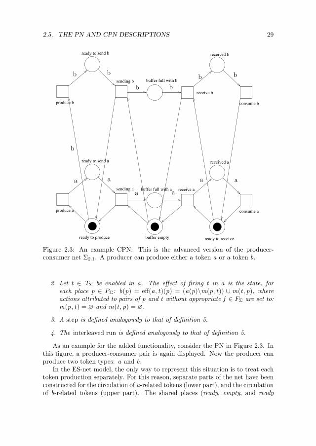
Figure 2.3: An example CPN. This is the advanced version of the producer-consumer net Σ2.1. A producer can produce either a token a or a token b.
2. Let t ∈ TΣ be enabled in a. The effect of firing t in a is the state, foreach place p ∈ PΣ: b(p) = eff(a, t)(p) = (a(p)\m(p, t)) ∪ m(t , p), whereactions attributed to pairs of p and t without appropriate f ∈ FΣ are set to:m(p, t) = ∅ and m(t , p) = ∅.
3. A step is defined analogously to that of definition 5.
4. The interleaved run is defined analogously to that of definition 5.
As an example for the added functionality, consider the PN in Figure 2.3. Inthis figure, a producer-consumer pair is again displayed. Now the producer canproduce two token types: a and b.
In the ES-net model, the only way to represent this situation is to treat eachtoken production separately. For this reason, separate parts of the net have beenconstructed for the circulation of a-related tokens (lower part), and the circulationof b-related tokens (upper part). The shared places (ready, empty, and ready

30 CHAPTER 2. TOOLKIT
ready to send
buffer full
ready to receiveready to produce buffer empty
replacemen
produce
sending
receive
received
consume
xx
xx
xx
x : a, bFigure 2.4: A CPN representation of the PN Σ2.3. The token x inscribed into thearcs can take values from the set a, b.
recv.) now have each a non-deterministic choice of actions to take. The producerdetermines which action is taken at the beginning of the interleaved run. It canbe seen that analogous places exist in the two parts, so that pairs of analogousplaces exist, with one place intended to track the a token, and the other intendedto track the b token. The ES-net models are used in cases where only the tokenflow, and the firing sequence of the transitions is important. The cases in whichalso the meaning of each particular token on a place and not only the presenceor absence of tokens is important for the activation sequence, gives rise to theso-called Coloured Petri Net (CPN).
The CPN are obtained by identifying analogous places (the places that havesimilar functionality to some extent). These analogous places can be joined into asingle place, with separate markings for the tokens residing there. This operationis called folding and can be used to contract the PN model into an equivalent CPN.The ES-net underlying a given CPN model is called an inscribed net. For Σ2.3,the corresponding CPN is shown in Figure 2.4. The folded net shown registersthe flow of the token x that can take values from the set a, b. It thus subsumesΣ2.3. When one refers to a token x at some place A, it is denoted as A.x . If thereexists a sequence of transitions that, given the presence of tokens A.x and B .y(on places A and B , respectively) fire so that token C .z is produced, one writes:
A.x ∧ B .y → C .z
and reads: A.x and B .y causes C .z . Proof techniques for CPN that take intoaccount the state of the coloured net are analogous to that of the PN as givenbefore. Multiple linked causes relations can be expressed in terms of proof graphs,which show both the causal relationship and concurrent executions.

2.5. THE PN AND CPN DESCRIPTIONS 31
76540123p
τ //t
(a)
tτ //76540123
p
(b)
76540123p
oo τ //t
(c)
76540123p
•τ //
t
(d)
Figure 2.5: The access modes. (a) Removal. (b) Addition. (c) Lookup. (d)Inhibition.
Access Modes
Originally the flow relation of the CPN forms a directed graph over the union ofthe places and the transitions. The firing of a transitions t means the removal ofthe corresponding tokens from the incident places t , and the production of thecorresponding tokens to t (see Figure 2.5). These correspond to two differentplace access modes :
1. Removal. The removal access mode at place p ∈ Place for a token τ ∈Dataspace deletes τ from the place p (see Figure 2.5a).
2. Addition. The addition access mode at a place p for a token τ adds τ tothe place p (see Figure 2.5b).
These access modes are denoted by orienting the arrow of each element of theflow relation either away from a place (removal), or towards a place (addition).For practical reasons this semantics of the flow relation is extended to includenew access modes. The new access modes are introduced for practical purposesand it is here noted that they may be simulated by using the basic removal andaddition modes only. However, for brevity, they are used as follows:
1. Lookup. The lookup access mode allows a transition to examine the contentsof its incident place in search for a token of particular type. The lookupaccess mode is denoted by a double-headed arrow between a place and atransition (see Figure 2.5c).
2. Inhibition. The inhibition access mode prevents a transition from havingconcession if the incident place in question contains a token matching agiven template. The inhibition access mode is denoted by a dot-tailed arrowconnecting the incident place and the transition (see Figure 2.5d).
par

32 CHAPTER 2. TOOLKIT
2.6 CPN Simulation by a Blackboard
We turn to the specification of a system given by its CPN description in theZ-with-CPN notation. For this purpose, the CPN description is expanded toinclude a “universal” data type, called Dataspace.
[ Dataspace ]
The Dataspace type is the union of all the elements that can be obtained by usingthe basic types and a finite number of iterated aggregations.
The basic types of the CPN are Place, and Transition. The precise contents ofthe types will be specified later. Here they are parachuted into the specification.
[ Place,Transition ]
Flow == (Place ∪ Transition)↔ (Place ∪Transition)
The PN itself is defined by defining the triple (P : Place,T : Transition,F : Flow).
PNP : P Place; T : PTransition; F : Flow
∀ x , y : Place ∪ Transition •(x , y) ∈ F ⇒ (x ∈ P ∧ y ∈ T )∨ (x ∈ T ∧ y ∈ P)
The set of transitions that have the arcs pointing to a particular place p of Pis denoted as p, and the set of transitions pointed to the arcs emanating fromp is denoted as p. A similar rule holds for a transition t from T . The set ofplaces that have arcs pointing to t is denoted as t , and the set of places that arepointed to by arcs emanating from t are denoted as t. A transition t is enabled ifthere is a token on all the places from t . It fires by removing the tokens from tand placing a token on t. Firing a single transition is called a step. A (possiblyinfinite) sequence of steps is called an interleaved run. In general, more than asingle transition can be enabled in a given state, so different interleaved runs canoccur.
ΞPN ; : PPlace ∪ P Transition
∀ p : Place ∈ P •p = t : Transition | t ∈ T ∧ (p, t) ∈ Fp = t : Transition | t ∈ T ∧ (t , p) ∈ F
∀ t : Transition ∈ T •t = p : Place | p ∈ P ∧ (t , p) ∈ Ft = p : Place | p ∈ P ∧ (p, t) ∈ F

2.6. CPN SIMULATION BY A BLACKBOARD 33
A CPN is obtained from a Σ : PN , by introducing coloring consisting of anuniverse A and an action m. The universe A, for each place p ∈ PΣ, prescribesthe set of allowable values for tokens on p, the domain A(p). On each place, anannotation called a token can be drawn. The placement of tokens is called thestate, and a PN is usually given in terms of the token marking for the initial state.Placeand transitions can be marked with a label.
CPNPNA : Place → P Dataspacem : (Place ∪ Transition)2 → P Dataspace
domA = P∀ x , y : Place ∪ Transition •
(x , y) ∈ domm ⇒ (x ∈ P ∧ y ∈ T ) ∨ (x ∈ T ∧ y ∈ P)
The state of a Σ : PN is a set a(p), for each p ∈ P , such that a(p) belongs toA(p). For p ∈ P , a(p) = ∅ means that on the place p there is no token for agiven state. If the state of a PN Σ is given as a, a transition t ∈ T is enabled ina if t ⊆ a. An additional condition is that t 6⊆ a.
a : Place → PDataspace
∀Σ : CPN • p ∈ P ⇒ a(p) ⊆ A(p)
Now revert to the definition of Place. Each p ∈ Place can contain a subset oftokens from its universe A(p), depending on the CPN marking given by the state.
Placet : PDataspace
t = a(self ) [self is the instance of Place]
The Transition operates on a sequence of objects that pass the guard conditioncorresponding to the concession given to each place of the CPN. This conventionbinds the two specification languages in Z-with-CPN allowing the precise defini-tion of a concession for each of the places. Every t : Transition specifies a functionτ that maps a sequence of acceptable input tokens into a set of the acceptableoutput tokens.
Transitionguard : seqDataspace 7→ true, falseτ : seqDataspace 7→ seq(Dataspace × Place)
dom guard ⊆ m(self , self )
∀(x : seqDataspace, y : seq(Dataspace × Place)) ∈ ran τ •x ⊆ m(self , self ) ∧ guard(x ) = 1 ∧ y ∈ self
34 CHAPTER 2. TOOLKIT
2.7 Blackboard Semantics
The structure handling the modified requirements is the Distributed Blackboard(DB) (see [20]). In this structure, all partial result exchange between the mappedtasks is modeled as communication in terms of data objects, which are fetchedfrom a data space, an (abstract) collection of all constructable data objects. TheDB as implemented by us is based on top of the Cognitive Agent Architecture(COUGAAR) framework, and then extended to handle the issues outlined here.The DB properties are as follows:
1. Structure. The DB is a collection of identical Local Blackboards (LBs), thatcan hold an unbounded-size collection of distinct objects. Each node (PDA)has access to one local LB.
2. Modification. The local LB is modified by either adding new objects to it,or removing or modifying them.
The addition of new objects to the DB readily implements the addition ac-cess mode of the CPN (Figure 2.5b). The removal of an existing objectfrom the DB readily implements the removal access mode of the CPN (Fig-ure 2.5a). The modification of the objects can be implemented twofold. Itis either a removal followed by immediate addition, or it is a lookup (Fig-ure 2.5c), depending on whether the removal mechanism must be triggered,or not, respectively.
3. Production. A node can select a subset of objects in LB for export. Theseobjects are called products and the incident node is called the producer.
4. Consumption. A node can select a subset of the product data space toimport. The incident node is called the consumer.
5. Distribution. Whenever an object o is added to a local LB such that it isa member of the local production data space, the object o is delivered to allconsumers whose consumption data space contains o.
6. Annotation. An object can be annotated by meta-data, which are alwayscommunicated when an object is transferred between nodes. To emphasizesome property P that holds for an object o, we write o 〈P〉. To annotatethe object o with a version label “ver = 2”, one writes: o 〈ver = 2〉.
The Static Structure of the Local Blackboard
A LB consists of an object container, the Blackboard (BB), and a number offunctional units, the Knowledge Sources (KSs). A KS is activated if an appro-priate subset of the data space is contained by the LB. Each activated KS maymodify the contents of the LB. The KS activation is asynchronous, so a monitor

2.7. Blackboard SEMANTICS 35
must synchronize concurrent LB access. A single LB is a container, holding anarbitrary number of objects from a predefined universe:
Blackboard = [ blackboard : PDataspace ]
Each KS is a piece of business logic. A KS contains a functional unit, acceptingobjects as input and producing objects as output:
FunctionalUnit = [ f : seqDataspace 7→ seq1 Dataspace ]
The objects for dom f and ran f are supplied from the LB. dom f ≡ seqDataspacesince a self-activated functional unit need not have input parameters. But ran f isnever empty. The parameters for f are obtained from LB, where they are selectedby applying a predicate:
Predicate = [ execute : Dataspace → true, false ]
The predicate can filter objects from LB to only those interesting for a KS. Threeobject classes are distinguished: the added objects, the removed objects and thechanged objects. The added and removed objects are remembered in a similarschema:
AddOrRemoveItem = [ x : Dataspace | x ∈ Blackboard ]
AddItem == AddOrRemoveItem
RemoveItem == AddOrRemoveItem
whereas the change schema describes the object change on the blackboard, sothat:
ChangeItem == (x : Dataspace, y : Dataspace) |x ∈ Blackboard , y 6∈ Blackboard
All change items are grouped in a change set:
AddSet == x : AddItem RemoveSet == x : RemoveItem ChangeSet == x : ChangeItem
A Subscription collects all the change sets, and uses a Predicate to limit its scopeonly to a subset of LB content for which a Predicate evaluates to true.
Subscription == [ p : Predicate, a : AddSet , r : RemoveSet , c : ChangeSet ]
A KS is completely specified by the accompanying FunctionalUnit, the VoidFunc-tion invoked when a KS is activated, and the set of its Subscriptions.
[ VoidFunction ]

36 CHAPTER 2. TOOLKIT
KnowledgeSourcefu : FunctionalUnitexecute : VoidFunctionsubs : seqSubscription
In some implementations, such as Cougaar [10], a KS is called a Plugin after thename of the software component implementing the KS, so the short alias for aKS is:
Plugin == KnowledgeSource
The LB system is then assembled from the Plugins and the LB.
BlackboardSystem = [ bb : Blackboard ; plugins : PPlugin ]
The Dynamic Structure of the Local Blackboard
Changes to the blackboard are applied in atomic transactions. The objects of theAddSet are added to the LB, with the replacements for the items from the domainof ChangeSet. The objects removed from the LB are those marked to be removed(i.e. members of the RemoveSet and the members of the domain of ChangeSet).
Transaction = [ a : AddSet ; r : RemoveSet ; c : ChangeSet ]
inducing the change in the of the LB contents.
ApplyTransaction∆BlackboardSystemt? : Transactionto remove, to add : P Dataspace
to remove = r? ∪ dom c?to add = a? ∪ ran c?
bb′ = (bb\to remove) ∪ to add
∀ x : Plugin • x ∈ plugins∀ y : Subscription • y ∈ x .subs
local add = x : Dataspace | x ∈ a?; y.predicate(x ) = 1 local remove = x : Dataspace | x ∈ r?; y.predicate(x ) = 1 local change = x : ChangeSet | x ∈ c?;
y.predicate(second(x )) = 1 y.a′ = local add ; y.r ′ = local remove; y.c′ = local change
Each Subscription is updated by updating its change sets. After these havebeen formed, each Plugin is invoked with the appropriate change set by executingthe VoidFunction.

2.8. CPN SIMULATION WITH A BLACKBOARD 37
InvokePlugin∆Plugin
execute
2.8 CPN Simulation with a Blackboard
In this section, the CPN and the BB concepts, described in the Sections 2.6 and 2.7respectively, are brought together to form a fully-fledged toolkit for specifying,describing and implementing distributed systems. The approach presented hereis of course but one of many that can be adopted in distributed systems design.The aims of the described toolkit are as follows:
1. Structuring. The way that a distributed system component is specifiedmust be expressed in an approved normal form which clearly expresses thebusiness logic and the concurrency of the distributed task.
2. Compilation. The structured specification must be convertible into an exe-cutable system description by an automated process and (possibly) an au-tomated compiler.
3. Verification. The structured specification must be amenable to manual orautomatic verification.
The toolkit can be viewed as a way of enforcing an engineering discipline intodistributed systems design. The discipline we give here is naturally not the onlyone you could adopt for building own distributed systems, and is certainly notthe only one that yields a functional system. However, a disciplined approachto engineering the distributed systems yields understandable designs, which canthen be checked against a number of quality-of-service requirements. Such callsfor programming discipline have been many, of which we give here some of themost prominent to our finding:
1. Structured programming [26] is based upon the notion that programs canbe composed of the fragments, which include statements and several well-defined flow-control structures. Each such fragment can have a single entrypoint and a single exit point1.
2. Object-oriented programming is based upon the notion that computer pro-grams are composed of objects that send messages to each other.
3. Design patterns [35] are based upon the notion that certain object instanti-ations and their connection recur in object-oriented program designs. The
1This strict view, due to Dijkstra [26] got an extension which allows the code to havemultiple exit points. Despite this disagreement about the exact formulation of the structuredprogramming approach, the general principle is nowadays almost exclusively used in practice.

38 CHAPTER 2. TOOLKIT
recurrent structures (patterns) are promoted as building blocks for well de-signed programs.
All can be used to structure the system design presentation, at the expense oflimiting the number of alternative ways to express a particular set of programmingactions. The advice given here is comparable in nature to those of structuredprogramming, the object-oriented programming, or the design patterns approach.It is an answer to the question: What have we learned about building reliable andverifiable distributed systems?
For the structured distributed system description, the following componentsare adopted:
1. Concurrent Events. The distributed state and the event concurrency aredescribed using the CPN formalism.
2. State Transitions. The concurrency description is augmented by the statetransitions, described in the Z notation.
3. Target Architecture. The target system architecture is a BB system, withthe BB semantics as given in the Section 2.7.
The conversion from the CPN description is illustrated with a classical “DiningPhilosophers” puzzle, due to Dijkstra[27].
“Five philosophers, numbered from 0 to 4 are living in a housewhere the table is laid for them, each philosopher having its own placein the table. Their only problem—besides those of philosophy—is thatthe dish served is a very difficult kind of spaghetti, that has to beeaten with two forks. There are two forks next to each plate, so thatpresents no difficulty, as a consequence, however, no two neighborsmay be eating simultaneously.”
The conversion is presented from the CPN description of the Dining Philosophersproblem to an implementation that uses the BB as the target architecture. How-ever, no special handling is provided to guarantee any of the classical constraints2.The presented implementation can be extended to incorporate an arbitrary strat-egy that does coordinate the philosophers’ activities and conforms to the classicalconstraints.
Concurrent Events
The first step in the specification is to determine the set of local states, and theallowed transitions between them. This amounts to the determination of the P ,
2The classical constraints [19] are: fairness, symmetry, economy, concurrency and bounded-ness.

2.8. CPN SIMULATION WITH A BLACKBOARD 39
T and F components of the PN scheme. In the Dining Philosophers dataspacethere are only two types:
[ Philosopher ,Fork ]
so that:
Philosopher = pi | i ∈ 0, 1, 2, 3, 4 Fork = fj | j ∈ 0, 1, 2, 3, 4
Therefore, the Dataspace is in this case:
Dataspace == Philosopher ∪ Fork
As the forks are set between the philosophers so that there is a single fork betweeneach pair of the neighbours at the table, one can define the functions giving thefork being laid left of, or right of, each given philosopher.
l , r : Philosopher → Fork
l = p0 7→ f0, p1 7→ f1, p2 7→ f2, p3 7→ f3, p4 7→ f4r = p0 7→ f4, p1 7→ f0, p2 7→ f1, p3 7→ f2, p4 7→ f3
Each philosopher can either be thinking or eating. These states alternatefor each given philosopher, although the interleaving of the states across all thephilosophers can vary. We can make the philosopher states explicit by adoptingplaces Thinking and Eating.
Thinking,Eating : Place
Similarly, a fork can be either available or busy, and the alternation and in-terleaving are similar as in the case of the philosophers. The states of the forksand the philosophers are not independent, however. If a token p ∈ Philosopher isin the state Eating, the forks l(p) and r(p) must not be in Available.
⊢ ∀ p : Philosopher • p ∈ a(Eating)⇒ l(p) 6∈ Available ∧ r(p) 6∈ Available
The converse does not hold, in the sense that the absence of a fork from Availabledoes not uniquely define the philosopher:
⊢ ∀ f : Fork • #l∼(f ) = 2, #r∼(f ) = 2
Therefore a local state representation with three places is in order for fully en-coding both the states of the forks and the philosophers. The additional place forthe forks is Available.
Available : Place

40 CHAPTER 2. TOOLKIT
Each philosopher starts by thinking. He is then taking the forks if availableand starting to eat. After a while, he leaves the forks and re-enters the thinkingstate. Hence two transitions are needed: Take and Leave.
Take,Leave : Transition
When defining the flow relation, it is natural to consider that any Take tran-sition must involve a previously thinking philosopher and his two adjacent forks.Hence the Take must have both the Thinking place and the Available place aspreconditions. The Take places the philosopher to the Eating state.
A converse process happens once a philosopher stops eating. The ensuingtransition is called Leave. Thus it must have the Eating as its precondition. Leavereturns the philosopher and the forks back to their original states (Thinking andAvailable, respectively). The resulting PN is given below.
INITPN
P = Thinking,Eating,AvailableT = Take,LeaveF = 〈Thinking,Take〉, 〈Available,Take〉,〈Take,Eating〉, 〈Eating,Leave〉, 〈Leave,Available〉, 〈Leave,Thinking〉
76540123Thinking
Leave //
//
76540123Available
// Take
oo76540123Eating
OO
Figure 2.6: The PN fragment that is obtained from considering the places andthe transitions only.
The PN given in Figure 2.6 is now coloured to obtain the complete CPNmodel. According to the exposition of Section 2.6, for this one needs to define theuniverse set A and the marking.

2.8. CPN SIMULATION WITH A BLACKBOARD 41
CPN InitΞCPN
A = Thinking 7→ Philosopher ,Available 7→ Fork ,Eating 7→ Philosopher
In the initial state all the forks are available, and all the philosophers arethinking.
a = Thinking 7→ p0, p1, p2, p3, p4,Available 7→ f0, f1, f2, f3, f4,Eating 7→ ∅m = 〈Thinking,Take〉 7→ x : Philosopher,〈Available,Take〉 7→ l(x ), r(x ),〈Take,Eating〉 7→ x : Philosopher,〈Eating,Leave〉 7→ x : Philosopher,〈Leave,Available〉 7→ l(x ), r(x ),〈Leave,Thinking〉 7→ x : Philosopher
We obtain the CPN as shown in Figure 2.7.
_^]\XYZ[p0p1p2
p3p4
Thinking x
Leave
l(x)
r(x)//
x
44
_^]\XYZ[f0f1f2f3f4
Available
l(x)
r(x)//
Take
x
pp76540123Eating
x
PP
Figure 2.7: The obtained CPN and the initial marking.
State Transitions
The transformations described by each transition can only be triggered if a tran-sition has a concession (i.e. is enabled). This occurs for a transition t : Transitionwhen a subset of tokens on t satisfies the guard condition of t (see Figure 2.8).For the guard condition of t , the following triggering condition must hold. The
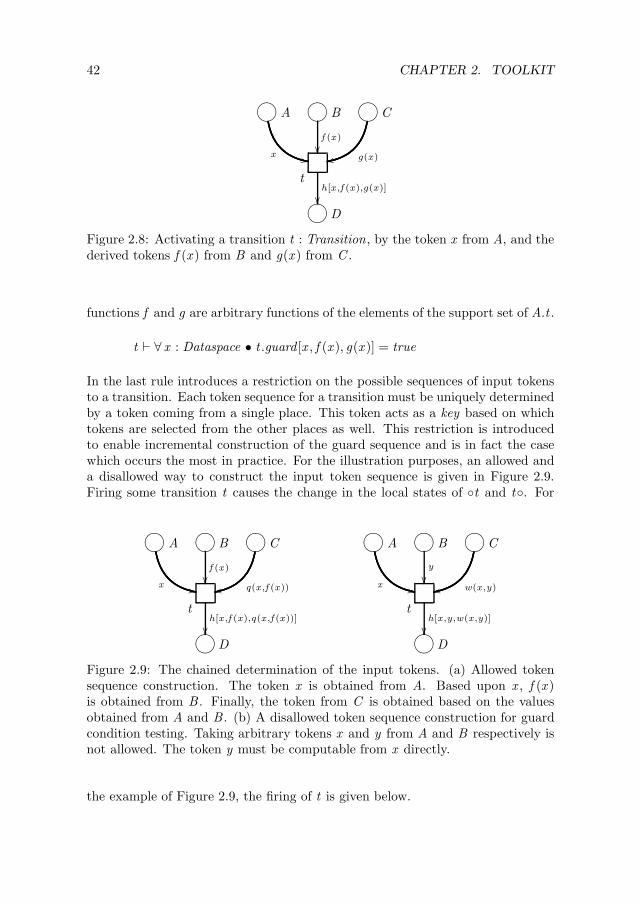
42 CHAPTER 2. TOOLKIT
76540123 A
x ,,
76540123 B
f (x)
76540123 C
g(x)rr
th[x ,f (x),g(x)]
76540123 D
Figure 2.8: Activating a transition t : Transition, by the token x from A, and thederived tokens f (x ) from B and g(x ) from C .
functions f and g are arbitrary functions of the elements of the support set of A.t .
t ⊢ ∀ x : Dataspace • t .guard [x , f (x ), g(x )] = true
In the last rule introduces a restriction on the possible sequences of input tokensto a transition. Each token sequence for a transition must be uniquely determinedby a token coming from a single place. This token acts as a key based on whichtokens are selected from the other places as well. This restriction is introducedto enable incremental construction of the guard sequence and is in fact the casewhich occurs the most in practice. For the illustration purposes, an allowed anda disallowed way to construct the input token sequence is given in Figure 2.9.Firing some transition t causes the change in the local states of t and t. For
76540123 A
x ,,
76540123 B
f (x)
76540123 C
q(x ,f (x))rr
th[x ,f (x),q(x ,f (x))]
76540123 D
76540123 A
x ,,
76540123 B
y
76540123 C
w(x ,y)rr
th[x ,y,w(x ,y)]
76540123 D
Figure 2.9: The chained determination of the input tokens. (a) Allowed tokensequence construction. The token x is obtained from A. Based upon x , f (x )is obtained from B . Finally, the token from C is obtained based on the valuesobtained from A and B . (b) A disallowed token sequence construction for guardcondition testing. Taking arbitrary tokens x and y from A and B respectively isnot allowed. The token y must be computable from x directly.
the example of Figure 2.9, the firing of t is given below.

2.8. CPN SIMULATION WITH A BLACKBOARD 43
Fire t∆A,B ,C ,D
x? : Dataspace
A.t ′ = A.t\x?B .t ′ = B .t\f (x?)C .t ′ = C .t\g(x?)D .t ′ = D .t ∪ h[x?, f (x?), g(x?)]
Returning to Figure 2.7, the definition of the CPN for the dining philosophersproblem is given as follows. For the firing of the Take transition:
Take∆Thinking,Available,Eating
x? : Philosopher
Thinking .t ′ = Thinking .t\x?Available .t ′ = Available .t\l(x?), r(x?)Eating .t ′ = Eating .t ∪ x?
For the firing of the Leave transition:
Leave∆Thinking,Available,Eating
x? : Philosopher
Eating .t ′ = Eating .t\x?Available .t ′ = Available .t\l(x?), r(x?)Thinking .t ′ = Thinking .t ∪ x?
Arbiter Transform for Non-Deterministic Transition Firing
In this section we treat the explicit arbiter insertion for the non-deterministictransition firing. In a CPN specification of a distributed process, the issue ofnon-deterministic choice remains open. The non-deterministic choice arises whenmultiple transitions are competing for the same token (see Figure 2.10). As faras the CPN semantics is concerned, an arbitrary resolution of the conflict yieldsa valid run fragment. This property naturally follows the way the CPNs are de-fined. However it is not immediately useful for the programming as it implies thestrong coupling between t1 and t2 and cannot be performed in a system basedon transactions without external arbitration. Hence in the implementation thearbiter must be explicit. However, the implementations will necessarily differ de-pending on whether the arbitration is fully contained in a single node, or whether

44 CHAPTER 2. TOOLKIT
76540123• p
???
????
?
t1 t2
(a)
76540123p
//t1
(b)
76540123p
//t2
(c)
Figure 2.10: The non-deterministic choice on a colourless PN and the respectiveinterleaved runs. The domain of the only place p is just A(p) = •. (a) TheCPN fragment with non-deterministic choice involved. (b) A run with t1 firing.(c) A run with t2 firing.
it is distributed. In case of the contained arbitration, usually not more than aselection is enough to direct the tokens to at most one of the enabled transitions.In case of distributed arbitration, provisions must be made so that the arbitra-tion remains manageable, and is not dominated by any participating party. Thisconcern is addressed when a distributed arbiter is made in Chapter 6, as a partof the Meet protocol design.
Another example of the non-deterministic decision is the mutual exclusion(mutex ) primitive. In the most basic mutex setting (see the PN Σ2.11 in Fig-ure 2.11), there exist two processes i ∈ 1, 2, each of which alternates between apending state (Pi) and a critical state (Ci), performing the enter (ei) and leaveli . The mutex requirement states that the processes must not simultaneously bein the critical state. The mutex requirement of Σ2.11 translates to:
e1
e2
76540123• P1
22
76540123 C1
rr
76540123 C2
,,
76540123• P2
ll
l1
RR
l2
LL
Figure 2.11: The setup for the mutex problem (Σ2.11).
Σ2.11 ⊢ C1 + C2 ≤ 1
Disregarding the non-determinism, the given mutex problem is solved by intro-ducing a shared place M as shown in Σ2.12. Inserting the place M to the network

2.8. CPN SIMULATION WITH A BLACKBOARD 45
Σ2.11 introduces the invariant:
Σ2.11 ⊢ C1 + C2 + M = 1
from which the required mutex condition is derived:
Σ2.11 ⊢ C1 + C2 + M = 1 ∧ M ≤ 1⇒ C1 + C2 ≤ 1
The way the contention between e1 and e2 is resolved is left unspecified and
e1
e2
76540123• P1
22
76540123 C1
rr
76540123• M
oo //
76540123 C2
,,
76540123• P2
ll
l1
RR BB
l2
LL\\
Figure 2.12: The non-deterministic mutex solution to Σ2.11.
in the PN definition, these ties are broken arbitrarily. Hence no guarantees canbe made upon the properties of the tie resolution. This is a hindrance to theimplementation where it is oft required that the ties are broken according tosome desirable pattern to ensure fairness, for instance. Breaking the ties is left toa device that we here call the arbiter. The arbiter decides which of the possibleruns is brought about and must be represented explicitly. In the case of Σ2.12,the arbiter is supposed to be intrinsic to both e1 and e2, implying that the twotransitions must be coupled. This contradicts the requirement that the transitionse1 and e2 must be the parts of independent processes. Hence a first take on thearbiter is to factor the decision out of the transitions ei (for i = 1 and i = 2) toyield Σ2.13.
Target Architecture
Here the conversion of the Z-with-CPN-based description of a distributed systeminto an executable component is described, such that the description is readilypluggable into an existing distributed system framework. The framework of in-terest in this writing is COUGAAR. In COUGAAR the complete application isdistributed across multiple hosts, where each is capable to execute a number ofrelatively independent entities of control. These entities are called agents in theCOUGAAR glossary and we adopt the naming here too.
A COUGAAR agent consists of a number of hierarchically ordered compo-nents. The components that make up a COUGAAR agent are listed in the speci-fication (called the society file), containing a recipe for the assembly of the agent.

46 CHAPTER 2. TOOLKIT
e1
76540123A1
oo π
a1
oo π
a2
//76540123A2
//e2
76540123• P1
22
76540123 C1
rr
76540123• M
ll 22
76540123 C2
,,
76540123• P2
ll
l1
RR ;;
l2
LLcc
Figure 2.13: Introducing a simple arbiter into Σ2.12. The arbiter is shown bydotted line. The predicate π and its complement π are used to decide whichprocess will be granted to the critical section.
The components are bound together by exporting services, thereby effectivelyrealizing the Inversion of Control (IoC) pattern (see [10] for the schematic viewof the COUGAAR agent components). The most important component for theapplication writer is the plugin. The plugins are able to access the internal agentblackboard and are meant to encompass the agent’s main business logic.
When implementing a given Z-with-CPN description of a distributed system,the designer must decide how to allocate and map the portions of the CPN de-scription to plugins. We feel it reasonable to leave the decision to the applicationauthor, as there is much freedom of choice in this matter. Our finding is that thefunctionality typically given in the form of several loosely coupled CPNs shouldbe implemented so that the tightly coupled parts reside in the same plugin.
As the plugins are the containers of the basic business logic of a COUGAARagent, the plugin structure does not necessarily reflect the logical grouping ofthe functionality as intended by the application author. In order to allow thefunctionality grouping on a sub-plugin level, we implemented the container object.The more detailed look at the main ingredients in the implementation of the CPNfor COUGAAR can be found in the Figure 2.14.
We now examine the implementation in somewhat more detail. The top levelCOUGAAR component is the TransitionContainerPlugin. This component at-taches directly to the COUGAAR infrastructure and, provided that it is correctlyinitialized with sub-components, performs all the housekeeping needed for thecorrect initialization of the CPN transitions.
A place in the CPN description must be represented in the implementationby an instance of a class Place. A transition must be represented in the imple-mentation by an instance of a class Transition. A Transition is connected to thecontainer using the following steps:
1. Activation or connecting the transition to other transitions by using theTrigger objects.

2.8. CPN SIMULATION WITH A BLACKBOARD 47
Transition+Transition():Transition+setTransitionSupport(support:TransitionSupport)+addTrigger(t:Trigger):Transition#execute(arguments:Map)#init()+getTriggerIterator():Iterator#getTransitionSupport():TransitionSupport+getName():String+setName(name:String)+toString():StringTransitionContainer#containerID:UID#transitions:List+TransitionContainer(containerID:UID):TransitionContainer+getTransitions():List+addTransition(t:Transition)+addTransitions(c:Collection)+getUID():UID+setUID(uid:UID)
TransitionContainerPlugin#transitionListSubsMap:Map#subscriptionTriggerMap:Map#triggerSubscriptionMap:Map#transitionList():List#execute()#onExecute()+load()#initTransitions()#initMarking()#setupSubscriptions()#connectSubToTrigger(subscriptions:List,trigger:Trigger,sub:IncrementalSubscription)+addTransitionContainer(tc:TransitionContainer)#addTransition(t:Transition)#Support():class+getBlackboard():BlackboardService+getUIDService():UIDService+getIdentificationService():AgentIdentificationService
Trigger+Trigger(place:Place,guard:Guard,predicate:UnaryPredicate,m:AccessMethod):Trigger+toString():String Guard#processed:Set+Guard(name:String):Guard#getName():String+execute(blackboard:BlackboardService,subscription:IncrementalSubscription,argumentMapList:List):boolean#initProcessed()#addProcessed(o:Object)#isProcessed(o:Object):boolean#getArgMap():Map
TransitionToken#name:String+TransitionToken(name:String):TransitionToken+getContent():Object#setContent(content:Object)+toString():String+getName():String
Figure 2.14: The main classes in the implementation of the Z-with-CPN specifi-cation on a blackboard-based architecture.

48 CHAPTER 2. TOOLKIT
2. Registration or inserting into the TransitionContainer of choice.
The transition activation, and all the subsequent operations are performed on thetransitions and places by symbolic name. Hence, a unique symbolic name must beprovided for all the places and transitions upon their initialization. This approachhas been adopted to allow forward referencing of the places and transitions duringthe CPN construction. The activation is performed by supplying the Transitionwith a number of Trigger objects. A trigger is always bound to some place andrequires the following specifications to be present:
1. Guard which validates an argument list (i.e. the set of tokens) and, ifvalidated, allows the transition to be invoked;
2. Predicate which filters the tokens that come from a particular place; and
3. Access method which specifies what change to the token set will be rele-vant for triggering the transition (the access methods were explained in theSection 2.5). The access method can be one of add, remove, change.
A Guard is executed each time a Trigger detects an access method to a black-board subset which has been registered with the corresponding Transition. Itstask is to build the argument list up. It iterates over the interesting places, insequence, and incrementally builds up a sequence of key-value tuples which willbe submitted to the transition when it fires. As the preconditions of the tran-sition are required to be derived from a common key, it is possible to build upthe argument list by incrementally invoking the registered Guard objects for thegiven Transition. Each Guard object is then forwarded the partial tuple sequenceto which elements are added according to the firing rules. The Guard can theneither expand the tuple, or it can remove it from the argument list.
Hence, the order of the Guard invocation is significant, and the applicationauthor must take care to register the guards in the sequence that retains theintended semantics from the Z-with-CPN description.
2.9 Summary
In this Chapter we equipped ourselves with the toolkit required to represent,specify and finally implement the DWEAM system. The presented toolkit will beused extensively in the following Chapters without further elaboration.

Chapter 3
Architecture Overview
This chapter gives the overview of the DWEAM system. The purpose of theexposition is to present in an integrated fashion the important aspects of theDWEAM system and its components. The components themselves will be detailedin future Chapters.
3.1 Introduction
Mobile computers are distinguished from their timely counterparts in that inmost applications the outcome of the execution is affected by the influence of theenvironment. A mobile computer is carried by a user that makes intermittentprocessing requests. Fulfilling the processing request requires the use of externalresources. The simplest use cases are placing a call from a cellular phone, or usingGeneral Packet Radio System (GPRS) to access an Internet web-site.
With respect to the computing resource mobility and the type of the network-ing interconnection, one can identify the following use cases (see Table 3.1):
1. With respect to the computing resource mobility:
a) Stationary, where the computing nodes generally remain at designatedconfined space, such as the home or office desktop;
b) Mobile, where the computing nodes change position in time.
2. With respect to the type of the communication infrastructure:
a) Fixed, where the computing resources use a structurally fixed commu-nication network; and
b) Ad-hoc, where the communication structures are built and maintainedat runtime.
49

50 CHAPTER 3. ARCHITECTURE OVERVIEW
Table 3.1: The use cases for the networked computing resources, with respect tothe mobility of the computing nodes and the type of the networking infrastructure.
Nodes Networking
Fixed Mobile Fixed Ad-Hoc Example
X X Home or Office Internet: Web Appli-cations, Multi-Agent Platforms, Dis-tributed Computing, Desktop Group-ware
X X Wireless Home or Office Internet: WebApplications, Desktop Groupware
X X Cellular Mobile: Telephone calls,GPRS Internet
X X WiFi (Ad-hoc access mode)
With reference to Table 3.1, it is noted that most of the usage modes are well-covered by existing applications. However, the support for mobile computingresources using ad-hoc infrastructure has so far been incomplete.
The ad-hoc access mode of the WiFi1 protocol allows point-to-point linksbetween wireless nodes to be established. This in effect emulates the mediumaccess policy of the Ethernet. In the Ethernet, arbitrary pairwise connections canbe established.
For wireless networks, the pairwise connectivity is achievable in only a limitednumber of use cases. It stems from the way these networks are constructed. Theexistence of a wireless connection between two nodes depends on the followingfactors:
1. Proximity. The wireless connection is effected through repeated radio trans-missions by the sending end of the connection. The reception of a radiotransmission requires that the signal power at the receiving end can be dis-tinguished from any other interfering signal that is received simultaneously.As the signal power decreases, it becomes more difficult to isolate the wantedsignal from the interference with the increase in the distance of the commu-nicating end points. Thus, the further away from each other the endpointsare, the more difficult it is for the communication to be established. As aconsequence, a given node of a wireless network is likely to be connectedonly to the nodes in the close proximity.
2. Interference. The radio is a shared medium admitting multiple concurrentusers. Thus, a given transmission can coexist with several other unrelatedbut concurrent transmissions. Upon the reception of a given transmission,
1WiFi is the common name for the IEEE 802.11 standard

3.1. INTRODUCTION 51
it must be separated from all the concurrent transmissions which are notof interest. Although the success of the separation schemes varies withthe employed separation approach, the overall tendency is that the morepowerful the signals from the unrelated transmissions are, the more difficultit is to separate the useful signal.
The mobility of the nodes in the wireless network causes the proximity andthe interference to vary. Consequently, it also varies the structure of the wirelessnetwork. The number of achievable links varies with time for the Mobile Ad-hocuse case. The variations in the network structure cause disturbances that bubbleup to the application level. An application that relies on the known networkstructure can cease to operate properly.
For practically all the use cases that include stationary nodes and fixed net-working, the changes in the network structure happen so infrequently that theyare approximated out of the network model. Thus, also a clean separation ofconcern between the networking and the application layers is achieved. As longas this approximation is valid, the performance of the application built on top ofthe fixed networking models is satisfactory.
The wireless networks unfortunately break this assumption. Therefore theapplications intended for the fixed networking do not carry over into the domainof ad-hoc networks with success. This phenomenon is characterized in [89] wherethe first point in the analysis of the open problems in the wireless network realmis:
“Architectures have been primarily driven by a ‘point-to-point’ phi-losophy; we need to better understand a network viewpoint whereinnodes can cooperate intelligently taking advantage of the special prop-erties inherent in wireless communication.”
The following approaches to resolve the issue are in order:
1. Emulation. In this approach, the algorithms of the ad-hoc networking layerare designed so as to emulate the behavior of a fixed networking layer. Theadvantage of this approach is that for as long as the emulation is successful,the system components at the upper layers can remain unmodified. Thedisadvantage is that the emulation may impose severe constraints on theuse-case for the emulated network. A typical example of this is the GSMnetwork. While it is based on radio communication, the only allowed use-case is that where all the users are separated by only a single hop from thebase-station that provides fixed infrastructure access.
2. Re-engineering. In this approach, novel primitives are designed to accommo-date the novel use-case. The advantage of this approach is that it potentiallyopens doors to a range of new applications, which were previously not con-sidered due to the limitations of the respective use-cases. The disadvantage

52 CHAPTER 3. ARCHITECTURE OVERVIEW
is that the new approach may introduce incompatibilities with the existingset of system components and design techniques.
In this work we take the second approach, assuming that the benefits of the newuse-cases outweigh the disadvantages. Bearing in mind that this new approachrequires new system components and design techniques to be formulated, in thischapter we give an integrated account of the designed architecture. The presen-tation is intended to familiarize the reader with the features of the architecture.
3.2 Resources
Two resource types are considered: the computation resources (also: computers,nodes) and the communication resources (also: network).
Computation resources
The computation resources (nodes) considered here are general purpose comput-ers.
Each node can be distinguished from others nodes by an unique message ad-dress.
[ MessageAddress ]
ΦNode
address : MessageAddress
∀n : Node • n 6= this ⇒ n.address 6= address [Unique address]
Communication resources (network)
The communication resources are used to exchange message objects between re-sources. The communication have a limited physical range, which depends onthe position of the nodes in physical space. Each node can communicate directlyonly with a comparatively small number of neighbours. The notion of neighbour-hood here coincides to some extent with the nodes which are physically close toeach other. More accurately, it depends on the properties of the communicationmedium (radio) which depends on mutual distance, but also varies in time.
Although the nodes are equipped with unique message addresses, the addressescan only be used to send message objects between nodes that can communicatedirectly. Hence it is only useful to distinguish between neighbours. This may notbe always possible as the connection environment varies in time.
[ Time ]

3.3. LAYERING 53
We use the symbol now to denote the “present time”. The details of the treatmentof time are given in Section 4.4, on page 72.
now : Time
We assume that the reachability is always symmetric.
direct link : Node ×Node × Time
messages cannot be sent between n : Node and m : Node at now⇒ (n,m,now) 6∈ direct link
∀n : Node,m : Node •(n,m,now) ∈ direct link ⇒ (m,n,now) ∈ direct link
Most of the time we are interested only in the direct reachability at currenttime (now).
direct linknow : Node ↔ Node
direct linknow= (n : Node,m : Node) | (n,m,now) ∈ direct link
3.3 Layering
The system architecture is organized into four basic layers. Each of the layersin its own right consists of a number of components that define its functionality.For a diagram of the component inter-dependencies please refer to the Table 3.2.The layers are arranged from top to bottom. They bridge the gap from the user,and the need that the user wants the system to fulfill, to the technology used tofulfill these needs. Hence the topmost layers are problem domain specific, and thebottom layers are technology specific. Only the adjacent layers interact, as usual.The layer components are almost perfectly neatly stacked, and their relations aresimilar to the relations of the adjacent layers: only the adjacent components caninteract.
1. Application Layer (APL). The APL is the top-level system layer. Here wespecify which computational tasks we require the system to perform.
After the task has been specified, we define a sequence of systematic trans-forms that convert a task specification first into a workflow structure thatshows explicitly the decompositions of a task into subtasks, and the pairwiseprecedence relation between the subtasks.
Then the workflow is cast into an executable schema that is based on theCPN framework which describes the process concurrency, supplementedwith the language based on Z2 [78] to express the transformation of thelocal process state. The executable schema is then mapped to a collectionof computing resources that can execute it.
2Both CPN and Z are explained where appropriate.

54 CHAPTER 3. ARCHITECTURE OVERVIEW
2. Blackboard Logic Layer (BLL). The BLL layer contains the componentsthat resulted from the allocation of the executable schema to the collectionof computing resources.
3. Connectivity Layer (COL). The COL layer contains the components thatenable the DWEAM system to fulfill its main functionality. This layerprovides an infrastructure for the synchronization of distributed computingresources, as well as the token persistence needed for the extended preser-vation of the system soft state.
4. Infrastructure Layer (INL). The INL layer contains the components whichprovide the basic connectivity structure to the DWEAM system.
It starts from the maintenance of the elementary connectivity, in which eachhost has knowledge only of a small number of immediate neighbours. It thenbuilds a minimal communication structure allowing multi-hop connectivitybetween the hosts.
On top of this structure, a matching is performed. The matching providesthe service discovery, which is used to determine the required interconnec-tions between the hosts.
Table 3.2: The layering and component structure of the DWEAM system. Thelayering is presented from the topmost (APL), to the bottommost (INL). Towardsthe top, the layers are problem-domain oriented, and towards the bottom the lay-ers are technology-domain oriented. The layer components are stacked accordingto their orientation within the layers. The ENS and PE components both providea foothold for ENS and both use the SP component.
Layer Components
Application Layer (APL) Static Task Structure (STS)Workflow Structure (WS)Petri Net Mapping (PNM)Host Mapping (HM)
Blackboard Logic Layer (BLL) Logic Component (LOC)Blackboard (BB)
Connectivity Layer (COL) Event Notification System (ENS)Persistency Component (PE)Matching (MAT)
Infrastructure Layer (INL) Specification (SP)Connectivity (CONN)Neighbourhood (NG)
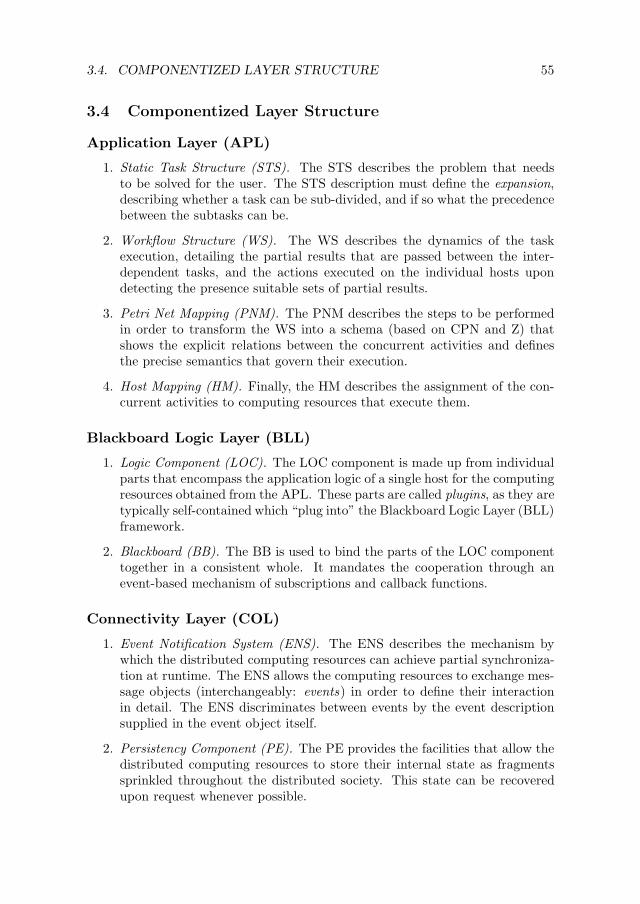
3.4. COMPONENTIZED LAYER STRUCTURE 55
3.4 Componentized Layer Structure
Application Layer (APL)
1. Static Task Structure (STS). The STS describes the problem that needsto be solved for the user. The STS description must define the expansion,describing whether a task can be sub-divided, and if so what the precedencebetween the subtasks can be.
2. Workflow Structure (WS). The WS describes the dynamics of the taskexecution, detailing the partial results that are passed between the inter-dependent tasks, and the actions executed on the individual hosts upondetecting the presence suitable sets of partial results.
3. Petri Net Mapping (PNM). The PNM describes the steps to be performedin order to transform the WS into a schema (based on CPN and Z) thatshows the explicit relations between the concurrent activities and definesthe precise semantics that govern their execution.
4. Host Mapping (HM). Finally, the HM describes the assignment of the con-current activities to computing resources that execute them.
Blackboard Logic Layer (BLL)
1. Logic Component (LOC). The LOC component is made up from individualparts that encompass the application logic of a single host for the computingresources obtained from the APL. These parts are called plugins, as they aretypically self-contained which “plug into” the Blackboard Logic Layer (BLL)framework.
2. Blackboard (BB). The BB is used to bind the parts of the LOC componenttogether in a consistent whole. It mandates the cooperation through anevent-based mechanism of subscriptions and callback functions.
Connectivity Layer (COL)
1. Event Notification System (ENS). The ENS describes the mechanism bywhich the distributed computing resources can achieve partial synchroniza-tion at runtime. The ENS allows the computing resources to exchange mes-sage objects (interchangeably: events) in order to define their interactionin detail. The ENS discriminates between events by the event descriptionsupplied in the event object itself.
2. Persistency Component (PE). The PE provides the facilities that allow thedistributed computing resources to store their internal state as fragmentssprinkled throughout the distributed society. This state can be recoveredupon request whenever possible.

56 CHAPTER 3. ARCHITECTURE OVERVIEW
3. Matching (MAT). The MAT is used to infer the resources which need tocommunicate the partial results of their tasks to each other. In order to dothis, the resources register a specification of the portion of the dataspaceinteresting for a particular resource, and the matching is performed throughdetermining which specifications have nonempty intersections.
Infrastructure Layer (INL)
1. Specification (SP). The MAT component depends on the SP mechanismto operate. The SP provides a language admitting a simple description ofdataspace subsets. By providing suitable set operations on dataspace sub-sets described by the use of SP, the MAT component is able to determinewhich computing resources need to establish a communication infrastruc-ture.
2. Connectivity (CONN). The CONN component assembles the basic NG-based connectivity and builds an elemental communication structure thatguarantees the minimum connectivity between any computing resources forwhich a connection can be found by following a sequence of NG connections.
3. Neighbourhood (NG). The NG component maintains a local list of all thecomputing resources which are directly reachable from some resource inparticular. Resources which do not see each other directly must to use theCONN for cooperation.
3.5 Component Overview
Here we give the specification of the DWEAM architecture components. Thepresentation of the components is bottom-up.
Neighbourhood (NG)
The NG component is installed at each node. The NG component maintains aset of neighbouring nodes as follows.
Φ2Node
ΦNode
neighbours : Time→ P Node
∀ t : Time,n : Node • (this ,n, t) ∈ direct link ⇒ n ∈ neighbours(t)

3.5. COMPONENT OVERVIEW 57
Connectivity (CONN)
The CONN component builds a minimal connectivity structure across all thenodes. The connectivity structure is a collection of mutually synchronized lo-cal states at all the nodes, such that the Connectivity property is satisfied (seeProperty 1 below).
The CONN first component that makes claims about the state of all the nodes.A pair of nodes that are not linked directly can still be reachable, if one can makea sequence of connected direct links between nodes.
reachable : Node ↔ Node
∀m : Node,n : Node • (m,n) ∈reachable⇒ (m,n) ∈direct link+now
The connectivity structure maintains the following invariant property.
Property 1 (Connectivity) Let m and n be nodes. Let m reachable n hold.The connectivity structure must provide that a message object sent from m, andhaving n as the destination, can reach n within finite time from the moment it issent.
In order to simplify the management of the CONN component, we require thatthe connectivity structure also be minimal.
Property 2 (Minimal Connectivity) The connectivity structure must be min-imal. No subset of the connectivity structure satisfies the Connectivity property.
The structure that satisfies Property 2 is called the Core Based Tree (CBT).The CBT is a compound structure distributed over the nodes, and the componentsof the structure are called uplinks.
Uplinkaddress : MessageAddress
The cardinalities of the sets of uplinks and downlinks are upper bounded bythe set of current neighbours. At most one uplink per node may exist.
ΦNodeLinks
uplinks : P Uplink
#uplinks ≤ 1
∀ u : Uplink • ∃n : Node •n ∈ neighbours ∧ u ∈ uplinks ∧ u.address = n.address
The uplink sets are synchronized between the neighbours. If a node has an uplinkwith an address of the neighbour, the corresponding neighbour must not have anuplink pointing the opposite way.

58 CHAPTER 3. ARCHITECTURE OVERVIEW
Property 3 (CBT) The CBT is either a:
1. Minimal weakly-connected directed graph on a set of all nodes and the setof all uplinks; or a minimal weakly-connected directed unicycle3 on a set ofall nodes and the set of all uplinks.
2. If the CBT is a tree, there is an unique node without an uplink, the core.If the CBT is a unicycle, there is no core, the cycle subset of the CBT isstrongly connected.
As mandated by the Property 3 and suggested by its name, the CBT resembleseither an oriented tree, or an oriented unicycle.
When two CBTs come into contact, they must be joined into a single CBT.The Property 3 holds for the resulting CBT. Since it takes time for the join oper-ation to complete, it is allowed that the CBT Property be temporarily violated.The frame in which this is allowed is called the Join transaction. For the jointransaction the following invariant holds.
Property 4 (CBT Join Transaction) For the join transaction for two CBTs:
1. During the transaction, Property 3 is satisfied in both CBTs;
2. After the join, Property 3 is satisfied for the resulting CBT.
Specification (SP)
The SP component defines the data modelthe DWEAM system. The SP consistsof sub-components:
1. Dataspace (DS). The DS is the space spanned by the constructable datatypes.
2. Specification (SP). The SP is a compact representation of the DS subsets.
Dataspace (DS)
The DS is informally described the set of all constructable types. A brief ac-count of the construction is given here, while Chapter 7 contains the detailedexplanation. Atoms are the common machine-dependent types.
Atoms ::= Naturals〈〈Z〉〉 | Reals〈〈R〉〉 | Strings〈〈seqCHAR〉〉
Constructors are used first to compose aggregate objects from the basic ones.The SchemaDefs represents the aggregate schema types and the Compounds are
3A unicycle with a unique closed path (i.e. cycle).

3.5. COMPONENT OVERVIEW 59
combinations of elements defined previously.
[ SchemaDefs ]
Compounds ::= Sets〈〈PCompounds ∪ Atoms〉〉| Sequences〈〈seqCompounds ∪Atoms〉〉| Schemes〈〈SchemaDefs〉〉
Next the schema definitions are given with SchemaDefs .
SchemaDefs ::= SingleSchema〈〈 〈| id : Dataspace |〉[id ]〉〉| MultiSchema〈〈〈| id : Dataspace |〉[id ]× SchemaDefs〉〉
Finally, the above components can be combined, completing the specificationof the Dataspace.
Dataspace ::= Atoms | Compounds | SchemaDefs .
Specification (SP)
The SP is used to represent portions of the DS. The SP summary is used topin down the DS context to which thereafter an operation can be applied. Anumber of operations on SP descriptions are defined, which admit the formationof compound summaries.
The summaries are used in the matching algorithm for finding the compatibleproducers and consumers.
[ Type ]
[ CHAR ]
Name == seq1 CHAR
The point in a DS is determined by specifying coordinates. Following the over-loading concepts from object-oriented languages, we allow multiple coordinateswith the same label. However, in order to distinguish between identically labeledcoordinates, a second attribute, the type is introduced.
[ Type ]
Textual representations of the types are all of the type Name.
Name == seq1 CHAR
A coordinate is then defined by its label and its type.
Coordinate = [name : Name; type : Type ]

60 CHAPTER 3. ARCHITECTURE OVERVIEW
Each Coordinate can take on any value from its support type. If we want toconsider only parts of the entire support set (denoted as X ), a constraint can bespecified.
Constraint [X ] == P X
Specifying a constraint for some coordinate yields a surface. Multiple surfaces onthe components of the same type X taken together, comprise a cube.
Surface == Coordinate × Constraint
Cube == PSurface
CompoundCube == PCube
The cube membership of a Dataspace point is defined through the use of thereflection operators.
∈ : Dataspace ↔ Cube
∈ : Dataspace ↔ CompoundCube
The required set operations are defined on cubes, and cube sets. Their defini-tion overloads the generic operations:
+ == ∪· == ∩· : Cube × Cube → Cube
· : Cube × CubeSet → CubeSet
· : CubeSet × CubeSet → CubeSet
The sharp operators [15] are defined in order to support the set operations oncubes.
[X ,Y ]# : Cube[X ]× Cube[Y ]→ CubeSet
©# : Cube[X ]× Cube[Y ]→ CubeSet
Analogous operations are valid for cube sets too.
©# : CubeSet2 → CubeSet
The availability of sharp operations enables the definition of the final, union op-erator for cube sets.
+ : CubeSet2 → CubeSet
All these operations are subsequently used in the (approximate) matching algo-rithm. At this point we omit the algorithm details, as its presentation containsseveral fine-grained details. The entire algorithm can be found in Chapter 7, onpage 145.

3.6. SUMMARY 61
3.6 Summary
In this Chapter we presented the DWEAM architecture in a nutshell. That is,we described the relevant properties of the used computation and communicationresources. Thereafter we moved on to the exposition of the system layers, andwithin each layer their specific components. All the layer components are thenexposed in brief, as the details of all of them are given in the Chapters that follow.


Chapter 4
Task Mapping
In this chapter, we describe the task mapping for DWEAM. Task mapping isthe name for a process that transforms the application requirements representedby a set of informally specified tasks into a specification that is executable in adistributed, dynamic computing environment. The steps required to perform thetask mapping are collectively referred to as Application Layer (APL).
The APL we describe is designed specifically (but not limited to) the appli-cations in emergency rescue operations, where the merits of the approach can befully appreciated. It can be thought of as an enabler for a crisis managementgroupware. The applications involve teams of individuals that need to act incoordination towards a common goal, and who use portable computers for ex-changing relevant information. While this is commonplace in command centers,the support for on-site communication leaves much to be desired. The presenteddesign offers a tool-chest that addresses this issue.
4.1 Introduction
What follows is a description of the APL design for a particular kind of a dis-tributed computing system. This APL addresses the issues arising when a dis-tributed computing system is deployed in an adverse environment. An adverseenvironment is such that it can have influence the course of the task execution,by shutting down the computational resources and changing the properties of thenetwork that connects the computers together.
A distributed computer system is a collection of connected computing resources.These resources execute coupled tasks and exchange intermediate results througha pre-installed network. Nowadays they come in a variety of packages—rangingfrom mainframe systems, through the familiar desktop computers, to the currentlyunder-represented but ever more penetrating portable devices as PDAs.
DWEAM is designed for the applications in emergency rescue operations. It isassumed throughout this article that a set of computational tasks suitable for this
63

64 CHAPTER 4. TASK MAPPING
purpose has been pre-defined and is executing concurrently as an aid to the maintask allocated to the emergency teams. The helper tasks can, for instance, be usedto report continuously of the progress of the main task, to request assistance orsupplies and report findings. Through the influence of the operating environment,the execution of these tasks can be affected. A task allotted to a single computercan fail if the computer is destroyed or detached from the network so that it isunable to communicate its data to the other computers in the network. This is incontrast to decision support information systems as deployed in command centers,where better guarantees on the reliability of the system and communication canbe assumed.
The task mapping we present prepares the tasks for the execution on a com-puter system that can cope with the influence of the environment and can executethe allotted tasks in a favourable manner (this informal description will formal-ized later in the text). Ideally, one wants to find a computational structure thatensures reliable and efficient computation regardless of the possible intermittentsystem faults. However, the achievability of this ideal goal is coupled to fun-damental impossibility results in distributed computing studies: in distributedcomputer systems that do not execute tasks in lock step, it is impossible to dis-tinguish a failed task from the one that is executing very slowly ([43]). Likewise,in face of communication failures ([51], Theorem 5.1). This result has far reach-ing implications for the system architecture, as it constrains the assistance to theresponse team that it can offer. Consequently, we are forced to relax the idealizedrequirement to meet realistic goals.
4.2 Requirements
The goal of the task mapping is to transform the desired system behaviour (ex-pressed by the set of tasks that we want it to perform) into business logic compo-nents1 executable by the available resources. The tasks of particular interest arethose supplemental to crisis management operations. It is assumed that the crisismanagement task is executed by a number of (personnel) units, that may be cou-pled by some kind of command chain. The structure of the command chain is notrelevant for this exposition. However, the support offered by the described sys-tem must be generic enough to accommodate the existing command and controlmethods.
In the following sections, we derive the distribution structure for the compu-tational tasks, starting from informal descriptions of prototypical tasks in crisismanagement. This is to motivate input from the crisis management researchcommunity to supply other appropriate applications. Thereafter we zoom intocomputational tasks within the crisis management domain and describe the STS.The dynamic task structure follows, and converted to CPN to structure it fully.
1That is, the executable program code which is structured so to be insertable as a componentinto a pre-defined software framework.

4.2. REQUIREMENTS 65
The section on task mapping gives the method to assign tasks to computerswhile preserving the task structure. The section on design constraints explainswhat threats prevent the maintenance of correct task structure, with our solutionand performance trade-offs. The section on distributed blackboard describes thestructure that supports the given requirements. A survey of related work follows,explaining the origins of the ideas we used in our exposition, and thereafter theconclusion is given.
Task Structure
We envision a near-future search-and-rescue operation, in which members of theparticipating emergency service units (police, fire brigade, ambulance, etc.) areequipped with PDA devices (nodes), each capable of short range radio communi-cation. These devices are used to exchange messages: findings, request backup,distribute orders etc. Only the devices within radio range can directly contacteach other. Devices which are connected indirectly, through successive connec-tions, rely on their neighbours to forward the messages. The network of nodesis constructed based on the connections created by a short range radio network:two nodes are connected if they are closer to each other than a pre-determinedrange. This assumption is shared by papers on wireless network properties, suchas [39].
We adopted a number of example operational tasks, to illustrate the type ofwork that is expected of the system to perform.
1. The distribution of orders down the command chain. In this example task,the system must support the distribution of orders. We assume a hierarchi-cal ordering of the available units, whereby the hierarchy is established interms of the command chain. The order is a data item (or: data object),generated at a single unit in the hierarchy, that must be distributed to allthe units that are its offsprings in the hierarchy tree.
2. The convergence of the order results up the command chain. In this exampletask, the system consists of a number of sensors emitting readings aboutthe environment. The convergence is the feedback of these readings to asingle node where the readings can be processed. The assumptions aboutthe hierarchy is the same as that of the previous task.
3. Cooperative map building. In this example task, the system must supportthe cooperative building of a site map. The entire team starts off with anempty, unannotated terrain map. Each team member can annotate the ter-rain map, taking note of newly discovered features. In a rescue operation,the annotations can signify sites where casualties are found, where the ter-rain conditions have changed from their default (due to debris for instance),or where logistic support (supplies) should be delivered. The annotationsmade by each team member are shared with others.

66 CHAPTER 4. TASK MAPPING
Static Task Structure (STS)
The tasks are twofold: the operational tasks are performed by actors (humans),and computational tasks that are performed by agents (computers). For the restof this exposition, only the computational tasks will be specially considered; weassume that a clean cut can be made to separate the task types, and that theyare easily conjoined when the system is deployed.
All the tasks require a coordinated set of actions to be performed by the teammembers. By each action, a part of the task (i.e. a subtask) is executed. Theexecution of an action brings about the subtask, and produces a partial result,which can be shared with the other team members. The coordination is achievedthrough synchronization, whereby different team members agree to execute theiractions in a certain order, and through cooperation, whereby the results of theoutcome of a single action are used to enable a subsequent action. We modelcoordination by messages exchanged by the team members, where each messagecontains a data object. A team member pends the action until an activationmessage is received (e.g. an order arrives to execute an action). When a messageis received, its contents are used in the action contents to execute the subtask.
The overall task is achieved by delegating subtasks to team members, andspecifying the way in which the subtasks interact with each other. For handlinga variety of tasks such as those of the example, we define the STS, with thedescription thereof relegated to a separate subsection.
Task Description
Tasks are described at mixed levels: informal descriptions given in English areused as needed to motivate formalization; formal symbolic descriptions are usedonce the task is described well enough to admit symbolic manipulation. The typeof the tasks is the opaque type Tasks. The computational tasks are applicationdefined. The messages are treated as coming from an abstract Dataspace.
[Tasks ,Dataspace]
Emphasize a single, top level task which contains the overall description of whatservice the system offers. This task is denoted as T where appropriate.
T : Task
Task Properties
1. Decomposition. A given task may be decomposed into a set of subtasks. It isassumed that many useful tasks in crisis management can be decomposed inthis way. Subtasks may be further decomposed until an elementary (atomic)subtask is reached.
TaskExpansionType == Tasks ↔ Tasks

4.2. REQUIREMENTS 67
→ : TaskExpansionType
An atomic subtask transforms objects by applying a transfer function fromTTF .
TasksToDataspaceFunction == Tasks → P(Dataspace → Dataspace)
TTF : TasksToDataspaceFunction
2. Activation. A task is started if a set of activation messages have beenreceived. Additionally, the set of received activation messages must satisfyall the guard conditions, which is a predicate on a set of objects. Uponcompletion, a task produces partial results, i.e. messages that can activateother tasks. The set of activation messages ACT , partial results PARTand guard conditions GUARDS are given by:
TasksToDataspaceSet == Tasks → P Dataspace
GuardType == Tasks → P(P Dataspace → true, false)
ACT , PART : TasksToDataspaceSetGUARDS : GuardType
A task which is not a subtask of any other is the top level task, and itspartial result is, at the same time, the (overall) result of the task execution.The top level task is executed if all of its subtasks have been executed. Anelementary task is executed if it has changed the system state according toits specifications.
3. Precedence. A precedence relation “≺” (read as: precedes) is established fortasks. For two tasks T and U , we denote T ≺U if and only if U is allowedto be executed only after T has been completed.
≺ : Tasks ↔ Tasks
∀(x , y) : Tasks2 • x ≺ y ⇔ x must be completed before y starts.
4. Coupling. Tasks T and U , where T ≺U are also coupled, if the partialresult of T is used as the activation message to U .
TaskRelation == Tasks ↔ Tasks
≺1 : TaskRelation
∀(x , y) : Tasks2 • x ≺1 y ⇔ (x ≺ y) ∧ [6 ∃ z : Tasks • (x ≺ z ) ∧ (z ≺ y)]

68 CHAPTER 4. TASK MAPPING
These coupled tasks are denoted as: T ≺1 U , and for them PARTT ∩ACTU 6= ∅. When the tasks T and U , are coupled, then by definitionthere exists no task V such that T ≺V ≺U . If, for two tasks T and Uneither T ≺U nor U ≺T , the tasks are decoupled, or concurrent. For thecoupled tasks, the activation property holds.
Property 5 (Activation)
⊢ ∀ x : Tasks , y : Tasks • x ≺1 y ⇔ PARTx ∩ACTy 6= ∅
The activation property expresses the coupling relation of T and U throughthe fact that the set of the partial results of T intersect the activation setof U .
The STS consists of the top level task T all the task property elements:
StaticTaskStructureT : PTasks ; → : TaskExpansionType, ≺1 : TaskRelation;TTF : TasksToDataspaceFunction; ACT , PART : TasksToDataspaceSet ;GUARDS : GuardType
STS : StaticTaskStructure
Dynamic Task Structure
The dynamic task structure is described in terms of a Petri Net (PN). The PNsgive a compact way to model and reason about the concurrent task execution. Wefirst present the PN and the derived Coloured Petri Net (CPN) model, and thendefine the EM, expressing the task structure in terms of an equivalent executableCPN.
4.3 Enabler Mapping (EM)
To transform a set of tasks into an executable structure, the EM is used. The EMconverts the STS to an equivalent CPN model, thus turning a static descriptioninto an executable schema.
EM : StaticTaskStructure → CPN
The function is total as any StaticTaskStructure must be convertible to a CPN.We specify EM constructively, in a sequence of steps that builds CPN componentsfrom a STS. For convenience, a renamed schema CPN [T/U ] is produced insteadof CPN as symbols T coincide in StaticTaskStructure and CPN . The renaming

4.3. Enabler Mapping (EM) 69
allows to drop the indices and consider only STS : StaticTaskStructure, andΣ : CPN [T/U ], for which the maplet STS 7→ Σ is within EM .
The maplet is built in a sequence of steps that together construct the compo-nents of the CPN Σ.
1. Retrieve atomic tasks. We need only consider atomic tasks. Non-atomictasks are complete automatically once all the tasks from their decompositionare complete.
atomic : PTasks
2. Define transitions. Make a transition for each atomic task. Additionally,attribute the transfer function to each transition.
trans : Tasks 7→ Transitiontrfun : Transition 7→ P(Dataspace → Dataspace)
dom trans = atomic
3. Define places. Define a place in P for any two coupled tasks from ≺1 .
places : Tasks × Tasks 7→ Place
dom places = ≺1
4. Define the flow. Define two components of the flow relation. First, the pre-condition component, connecting “inbound” Place to Transition. Second,the postcondition component, connecting Transition to “outbound” Place.
prec : (Tasks × Tasks)× Tasks 7→ Flowpostc : Tasks × (Tasks × Tasks) 7→ Flow
dom prec = x : Tasks × Tasks , y : Tasks | x ∈ ≺1 ∧ y ∈ dom xdom postc = x : Tasks , y : Tasks × Tasks | x ∈ ran y ∧ y ∈ ≺1
The flow relation is the union of these two components.
5. Define the universe. The universe is borrowed from the activation propertyfor coupled tasks.
6. Define the inscription. The inscription determines which transitions areenabled. The inscription on an arc connecting a place and a transition is aset of subsets of points in the data space for which all the guard predicatesare valid. The inscription on an arc connecting a transition and a place isa set of subsets of points from the data space.
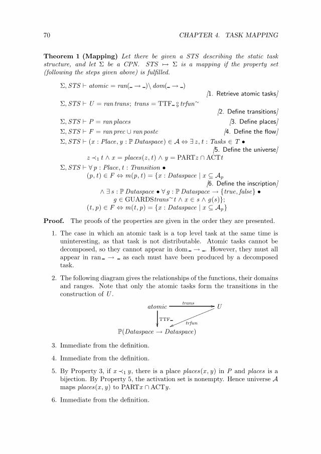
70 CHAPTER 4. TASK MAPPING
Theorem 1 (Mapping) Let there be given a STS describing the static taskstructure, and let Σ be a CPN. STS 7→ Σ is a mapping if the property set(following the steps given above) is fulfilled.
Σ,STS ⊢ atomic = ran( → )\ dom( → )[1. Retrieve atomic tasks]
Σ,STS ⊢ U = ran trans ; trans = TTF o9trfun∼
[2. Define transitions]
Σ,STS ⊢ P = ran places [3. Define places]
Σ,STS ⊢ F = ran prec ∪ ran postc [4. Define the flow]
Σ,STS ⊢ (x : Place, y : P Dataspace) ∈ A ⇔ ∃ z , t : Tasks ∈ T •[5. Define the universe]
z ≺1 t ∧ x = places(z , t) ∧ y = PARTz ∩ACTt
Σ,STS ⊢ ∀ p : Place, t : Transition •(p, t) ∈ F ⇔ m(p, t) = x : Dataspace | x ⊆ Ap
[6. Define the inscription]∧ ∃ s : P Dataspace • ∀ g : P Dataspace → true, false •
g ∈ GUARDStrans∼t ∧ x ∈ s ∧ g(s);(t , p) ∈ F ⇔ m(t , p) = x : Dataspace | x ⊆ Ap
Proof. The proofs of the properties are given in the order they are presented.
1. The case in which an atomic task is a top level task at the same time isuninteresting, as that task is not distributable. Atomic tasks cannot bedecomposed, so they cannot appear in dom → . However, they must allappear in ran → as each must have been produced by a decomposedtask.
2. The following diagram gives the relationships of the functions, their domainsand ranges. Note that only the atomic tasks form the transitions in theconstruction of U .
atomictrans //
TTF
U
trfunvvlllllllllllllll
P(Dataspace → Dataspace)
3. Immediate from the definition.
4. Immediate from the definition.
5. By Property 3, if x ≺1 y, there is a place places(x , y) in P and places is abijection. By Property 5, the activation set is nonempty. Hence universe Amaps places(x , y) to PARTx ∩ACTy.
6. Immediate from the definition.

4.3. Enabler Mapping (EM) 71
The properties 1 to 6 define Σ that corresponds to the given STS. The re-naming is reversed so that the maplet is type-compatible with EM .
Property 6 (Mapping rule) Let there be given an Enabler Mapping (EM), andlet there be given a Static Task Structure (STS), mapping the static task structuresinto the corresponding CPNs. Let Σ[U /T ] be a CPN obtained by applying thesteps from Theorem 1. Then
⊢ (STS 7→ Σ[U /T ]) ∈ EM
That is, STS 7→ Σ[U /T ] is a valid EM component.
Example 3 A form of this mapping can be found in the usual networked appli-cations. A web browser executes the task:
T == “display a web page”
for which
ACTT = Uniform Resource Locator (URL) input by the userand
PARTT = present the web page contents.Further, T decomposes as: → = (T ,T1), (T ,T2), (T ,T3), (T ,T4) , where:
T1 == “request page from the server given an URL”
T2 == “accept request for page”
T3 == “deliver page”
T4 == “accept page delivery”.
In this case T1≺1 T2≺1 T3≺1 T4. The coupling between T1 and T2 is achievedby setting PARTT1 = ACTT2 = o, where o ==URL. Other couplingsare given by PARTT2 = ACTT3 = request o, and PARTT3 = ACTT4 =page for o. The transfer functions are given as: TTF = T1 7→ τ1,T2 7→τ2,T3 7→ τ3,T4 7→ τ4 . The function GUARDS is empty.
Assume that there is a STS : StaticTaskStructrure with properties as givenabove. Now we find the elements of a corresponding Σ : CPN [T/U ]. TheProperties referred to here come from the theorem 1.
Σ,STS ⊢ (Property 1)⇒ atomic = T1,T2,T3,T4 By Property 2, there should be a transition per transfer function. These are givenby:
Σ,STS ⊢(Property 2)⇒
U = ran trans = ran TTF ∼ o9trans =
= t : Transition | ∃ τ ∈ ranTTF • t = TTF ∼ o9trans(τ) =
= t1, t2, t3, t4

72 CHAPTER 4. TASK MAPPING
with:
Σ,STS ⊢ trans = T1 7→ t1,T2 7→ t2,T3 7→ t3,T4 7→ t4
Also:
Σ,STS ⊢ (Property 3)⇒ P = places(T1 ≺1 T2), places(T2 ≺1 T3),places(T3 ≺1 T4) = p1, p2, p3
The flow relation is established using Property 4.
Σ,STS ⊢ (Property 4)⇒prec = ((T1,T2),T1) 7→ f1, ((T2,T3),T2) 7→ f2, ((T3,T4),T4) 7→ f3postc = (T2, (T1,T2)) 7→ f4, (T3, (T2,T3)) 7→ f5, (T4, (T3,T4)) 7→ f6F = fi : Flow | i ∈ 1 . . 6
The universe is determined from the activation message set:
Σ,STS ⊢ (Property 5)⇒ A = p1 7→ o, p2 7→ “request o”,p3 7→ “page for o”
and the inscriptions are analogously:
Σ,STS ⊢ (Property 6)⇒m = (t1, p1) 7→ o, (p1, t2) 7→ o,(t2, p2) 7→ “request o”, (p2, t3) 7→ “request o”,(t3, p3) 7→ “page for o”, (p3, t4) 7→ “page for o”
The resulting CPN is shown in Figure 4.1.
t1
o //76540123p1
o //
t2
requesto //76540123
p2
requesto //
t3
pagefor o //76540123
p3
pagefor o //
t4
Figure 4.1: The resulting Task Mapping, represented by a CPN.
4.4 Mapping Tasks to Nodes
The main purpose of the task distribution structure is the task to resources map-ping. The tasks are mapped via the CPN obtained from the Static Task Structure.Two resource types are considered. First, the computational resources (hereafter:nodes) which are able to execute the computational tasks. Nodes are hereafterdenoted by lower-case Greek letters.
[ Node ]
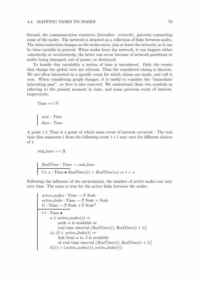
4.4. MAPPING TASKS TO NODES 73
Second, the communication resources (hereafter: network), pairwise connectingsome of the nodes. The network is denoted as a collection of links between nodes.The interconnection changes as the nodes move, join or leave the network, so it canbe time-variable in general. When nodes leave the network, it can happen eithervoluntarily or involuntarily; the latter can occur because of network partitions ornodes being damaged, out of power, or destroyed.
To handle this variability a notion of time is introduced. Only the eventsthat change the global view are relevant. Thus the considered timing is discrete.We are often interested in a specific event for which claims are made, and call itnow . When considering graph changes, it is useful to consider the “immediateinteresting past”, so then is also reserved. We understand these two symbols asreferring to the present moment in time, and some previous event of interest,respectively.
Time == N
now : Time
then : Time
A point t ∈ Time is a point at which some event of interest occurred . The realtime that separates t from the following event t +1 may vary for different choicesof t .
real time == R
RealTime : Time→ real time
∀ t , u : Time • RealTime(t) < RealTime(u)⇒ t < u
Following the influence of the environment, the number of active nodes can varyover time. The same is true for the active links between the nodes.
active nodes : Time→ P Nodeactive links : Time→ P Node ×NodeG : Time→ P Node × PNode2
∀ t : Time •α ∈ active nodes(t)⇒
node α is available atreal time interval (RealTime(t),RealTime(t + 1)]
(α, β) ∈ active links(t)⇒link from α to β is availableat real time interval (RealTime(t),RealTime(t + 1)]
G(t) = (active nodes(t), active links(t))

74 CHAPTER 4. TASK MAPPING
The nodes and links available at t : Time naturally induce a graph that is denotedas Gt . For G(now), and appropriate other denotations, indices can be dropped2.
Gt == G(t)active nodest == active nodes(t)active linkst == active links(t)G == Gnow
active nodes == active nodesnow ; active links == active linksnow
The transition mapping TRANS determines which nodes are allocated towhich transition. Multiple nodes may implement the same transition.
TRANS : Transition → P Node
A transition t : Transition mapped to some α : Node, is written as mappedto tα.Thus, mappedto tα and mappedto tβ are instances of the same transition, mappedrespectively to nodes α, and β.
The following requirements are imposed on the transition mapping for anyΣ : CPN :
1. The transition mapping must preserve the CPN structure. Consider transi-tions t , and u coupled by a place p:
Σ ⊢ p = µ q • q ∈ P ∧ t ∈ q ∧ u ∈ q
Then, a necessary condition for u to be executed is that the tokens fromp are deposited from t to p and then to u. When these transitions aremapped to nodes, such that mappedto tα and mappedto uβ, this means thatcommunication must be ensured between α and β so that the activation ofmappedto uβ is possible.
Σ ⊢ ∃ p ⇒ (TRANSt , TRANSu) ∈ active links
2. The mapping set for each transition must be non-empty. Every transitiont ∈ TΣ must map to at least one node in the set of active nodes.
Σ ⊢ TRANSt ∩ active nodes 6= ∅
Ensuring that these two necessary conditions hold is sufficient for the CPN exe-cution3.
2As a salient side effect to the arbitrary choice of the event corresponding to now , theproperties where items appear with indices dropped must hold for all possible choices of now .
3However, it is not sufficient to also validate the CPN with respect to safety and livenessproperties. Liveness and safety hold only if the CPN has been designed with these propertiesin mind.

4.4. MAPPING TASKS TO NODES 75
Example 4 We pick up Example 3 where we left off. A mapping to two nodesis given: active nodes = γ, δ, with active links = (γ, δ), where γ == clientand δ == server.
TRANS = t1 7→ γ, t2 7→ δ, t3 7→ δ, t4 7→ γ.
It is easy to inspect TRANS to verify that both properties hold.
Design Constraints
Fulfilling the task mapping requirements is complicated by the dynamic nature ofthe network formed by the nodes. As the owners of the PDAs move, the structureof the network changes, thus affecting the first transition mapping requirement.Furthermore, as PDAs are subjects to faults and destruction, the second transitionmapping requirement can be violated for a task T if all nodes in TRANST areaffected.
The loosely-coupled collection of PDAs, as outlined here, matches the asyn-chronous model of a distributed system being “separate components [taking] stepsin an arbitrary order, at arbitrary relative speeds” ([51], page 5). Two importantconstraints apply for such asynchronous systems:
1. Coordination is impossible under communication failures. This is the sim-ilar to the “coordinated attack problem” ([51], Theorem 5.1), establishingthat in a distributed system, with at least two communicating nodes, it isnot possible for the two nodes to agree over a value of a variable4 if com-munication can fail.
2. Slow and stopped nodes are indistinguishable. This observation ([43]) estab-lishes that nodes in an asynchronous system cannot determine if a particularother node has crashed, or is running slowly.
The given constraints affect the adherence to the transition mapping requirements.We call this influence a threat5.
The first constraint is a threat to the first transition mapping requirement.
Example 5 Consider transitions t, and u, and assume that p exists as given inthe first mapping requirement. The activation of some u : Transition depends onthe reception of all data objects from the inscription m(t , p) from t. When theseobjects are miscommunicated, the nodes α = TRANSt and β = TRANSu cannotagree whether the activation condition is fulfilled: α has sent m(t , p) so in α’sview u can be executed. But β has not received m(p, u), so in β’s view, u cannotbe executed.
4This is known as the “Consensus Problem” (see e.g.[30]). In the consensus problem, twoor more computers begin with an initial value of some type, and must eventually output a valueof that same type. The outputs of all the computers must be the same.
5The term “threat” is taken from AI planning domain ([72], Chapter 11), where it denotesan action that prevents the execution of a formulated partial plan.

76 CHAPTER 4. TASK MAPPING
Furthermore, as the nodes in G move, join and leave the network, a transientmapping threat can occur.
Example 6 (Transient mapping threat) Let there be two active nodes:
active nodes = α, β,
with transitions t and u, and a place p as given in the first requirement. Let thetransition mapping be constant TRANS = t 7→ α.
Let active links be variable, as follows. Assume that there are only threeevents: −∞, then, and now. These three events divide the real time into threeparts. Assume active links−∞ = (α, β). At then, the only link is broken so thatactive linksthen = ∅, and subsequently restored: active linksnow = (α, β). Byinspection one finds that the first requirement is violated in the interval (0, 1].
The second constraint is a threat to the second transition mapping require-ment.
Example 7 It follows that a transition t cannot check whether TRANSt = ∅, asa probe message sent to a node in TRANSt may receive a reply with unboundeddelay.
In the light of the design constraints, a system that adheres strictly to thetask mapping requirements is not achievable. We therefore consider a relaxed,probabilistic formulation of the transition mapping requirements, so that theyhold with high probability (whp)6. We adopt two simple structuring principlesthat achieve this.
1. Token Persistence. Instead of limiting the token communication to a certaintime frame, thus giving rise to transient mapping threats, the tokens arepresent indefinitely once generated. In [57] it is shown how this can beachieved whp.
2. Mapping Redundancy. The TRANS must map a transition to multiplenodes in G. The mapping set is shown to be nonempty whp in [29].
The structuring principles remove the threats, but introduce side effects, withper-application significance:
1. Excess Storage. The indefinite lifetime of the persistent tokens is not achiev-able in practical systems where the memory is always bounded. This obviousissue is handled in the standard systems by garbage collection.
6The term whp means that the probability that a requirement holds is a function of a positiveparameter n of the form 1 − 1
nk for some k > 1.

4.5. DISTRIBUTED BLACKBOARD 77
2. Duplication. Due to the mapping redundancy, it is possible that multiple,functionally equivalent tokens are produced at runtime. Given a transi-tion t and the mapping TRANSt = α, β, transitions mappedto tα andmappedto tβ produce equivalent partial results. This issue is handled byvisioning the partial results, so that they can be compared.
3. Redundant token deliveries. As a joint effect of token persistence, and thetemporal variation of active links , multiple deliveries of the same token,originating from the same node can occur. This amounts to the at-least-once message delivery semantics.
4.5 Distributed Blackboard
The Distribution Mechanisms (DMs)
The extension to the Local Blackboard (LB) is the Export Mechanism (EMX)allowing the copies of data space objects to be shared across multiple LBs, andthus be locally accessible to the active nodes.
The EMX is a new take on the familiar ideas of distributed shared memory andtuple spaces (see [3]). The distributed shared memory emulates a unique memoryspace to which several nodes can have concurrent access. Thus the nodes see thepossibly fragmented memory as an unique memory space. In the tuple spacesimplementation, the tuple space is a domain in which objects exist. An objectis instantiated by inserting it into the tuple space. After that it becomes visiblefor all the nodes attached to the said tuple space. Subsequent operations canmodify and delete such an object. The tuple spaces are associated with a notionof authority whereby only the resource that has inserted an object can modify it.
In the EMX, a modified approach is considered. Each node maintains anindependent local view of the data space. This is achieved by the LB and thelocal views can be freely modified according to the LB semantics. Cooperationbegins once a node marks a subset of its local LB Exported View (XV). The XVis what the node is willing to share with the environment.
In line with the structuring principles introduced earlier, several consequencesresult.
1. The implied required storage for all the XVs is unbounded, (in line with theexcess storage effect);
2. Once exported, an object cannot be deleted or modified (in line with theduplication effect);
3. As each node reports on its XV whenever asked, it is possible that it answersto the same inquiring node multiple times (in line with the redundant tokendeliveries effect).

78 CHAPTER 4. TASK MAPPING
Consider all nodes a client to the DB structure. Each client can express aninterest in a subset of the dataspace.
ClientInterest == P Dataspace
Although the client interest is defined as a subset of a possibly large dataspace, itis worth noting that encoding the interest can be much more efficient if only theboundaries of the interest are encoded.
ProducerΞBlackboardSystem
exported : ClientInterest
exported ⊆ blackboardbb
The node becomes a producer for the subset of the data space covered by exported .Any other node is free to ask for a subset of the exported view, making it aconsumer.
Consumerimported : ClientInterest
A node may produce some objects, and consume others (in line of the transi-tion mapping). The node name in this dual role is Client.
Client == Producer ∧ Consumer
The client is free to modify the exports and import interests at will.
ModifyProducer∆Producer
exported? : ClientInterest
exported ′ = exported?
Likewise for the consumer.
ModifyConsumer∆Consumer
imported? : ClientInterest
imported ′ = imported?
In the example we compare the conventional view to that of the DB.

4.5. DISTRIBUTED BLACKBOARD 79
Example 8 (Blackboard Bank Account) Consider a classical example of theconcurrent access7 to a project bank account8. Project participants can use themoney from the account to get equipment for the experiments. Alice (A) and Bob(B) each request 1e. The requests are forwarded to the Bank (X ).
X : N
A,B : Z→ Z
X = 2,X ≥ 0 [Account balance]
A = B = λ x : Z • x − 1 [Requests]
The Bank enforces that the account X is unique at all times and enforces the strictaccess semantics. Hence processing concurrent withdrawal transactions from Xrequires that a valid sequentialization exists. That is, an ordering of sequentialtransaction applications for which commonly understood semantics exist. Pro-vided enough funds are present, the bank applies the two transactions to the bankaccount, so that only the final balance is left. In this case there are two differentways to sequentialize, and these are equivalent from the Bank’s point of view.
(A o9B)X = (B o
9A)X = 0
In the modified case, X = 1, only one of the requests can be fulfilled, as faras the Bank is concerned. This would annoy either Alice, or Bob, but not bothas only one of the requests can be performed while keeping the account balancenon-negative.
Now turn to the Distributed Blackboard (DB) case. Regardless of the stateof the bank account, both requests can be executed on the account object, yield-ing a new state. All objects are simultaneously exported by the EMX of all theparticipants.
Question arises which of the produced objects is the “real” state of the projectaccount after concurrent accesses have been performed. Only all the objects con-sidered at once encode the full state. But, what is “real” depends on the viewpoint.Likely, from Alice’s point of view, AX being the real state is just enough. For whatwe know, the converse holds for Bob. And both would agree that it would be greatfor the original balance X to remain. What prevents these dreams from becomingtrue is the authority of the Bank. The authority is drawn from real finance thatthe Bank controls. A Bank signing some of the objects (denoted as: X) it means:“the Bank claims that this is the ‘real’ state”.
7The concurrent access to a shared variable is considered a classical example and is describedin many books. The blackboard bank account example is invented here, however.
8Such an account can have several researchers who independently and concurrently drawfunds from it.

80 CHAPTER 4. TASK MAPPING
Either9: AX 〈X〉
X 〈X〉
A
::uuuuuuuuu
B
%%JJJJJJJJJ
BX
or: AX
X 〈X〉
A
;;wwwwwwww
B
##GGGGGGGG
BXor: AX
A∼o9(Ao
9B)
&&MMMMMMMMMMM
X 〈ver = 1, X〉
A
88qqqqqqqqqqq
B
&&MMMMMMMMMMM//________ X 〈ver = 2, X〉
BX
B∼o9(Ao
9B)
88qqqqqqqqqqq
This prevents neither Alice nor Bob to still privately hope otherwise: no-oneprevents you to consider yourself rich when you are likely not10. But it does notdo any good to either of them (as the vendors are likely to believe the Bank) andthey might just as well accept the truth. As far as the storage for the objects isconcerned, in this context there is no incentive for anyone to remember the oldaccount state11 X given that the authority has updated.
This illustrates the important difference in the approaches that use DB tothose of the conventional transaction-based systems. On a DB, an object, onceposted is never removed or modified. When it becomes necessary to represent achange to the object on the DB, it is done by producing a similar object witha different annotation and maintaining a relation between objects which denoteshow the new object relates to the old. In the example, a version stamp (ver) andthe bank signature (X) are used. It is a matter of external convention to ensurethat the objects on the DB fulfill the constraints placed on them. The DB clientsare free to choose these conventions and even have several of them concurrentlyin effect.
4.6 Related Work
The motivation for the presented design is the introduction of automated deci-sion support systems for the crisis management domain all the way through the
9The blackboard arrow diagrams show possible blackboard contents at a given time. Thearrows show the production dependence, and the arrow inscription shows the transform thathas been applied to the source object to obtain the destination object.
10The meaning of “being rich” is relative and depends on what one sees as relevant for beingrich. We stay on the pragmatic track and not mandate that meaning. Instead we allow multiplemeanings to exist concurrently, and it is up to each participant to choose the one which isrelevant for the given context.
11The Bank may keep the records for own bookkeeping but these need not be exported.
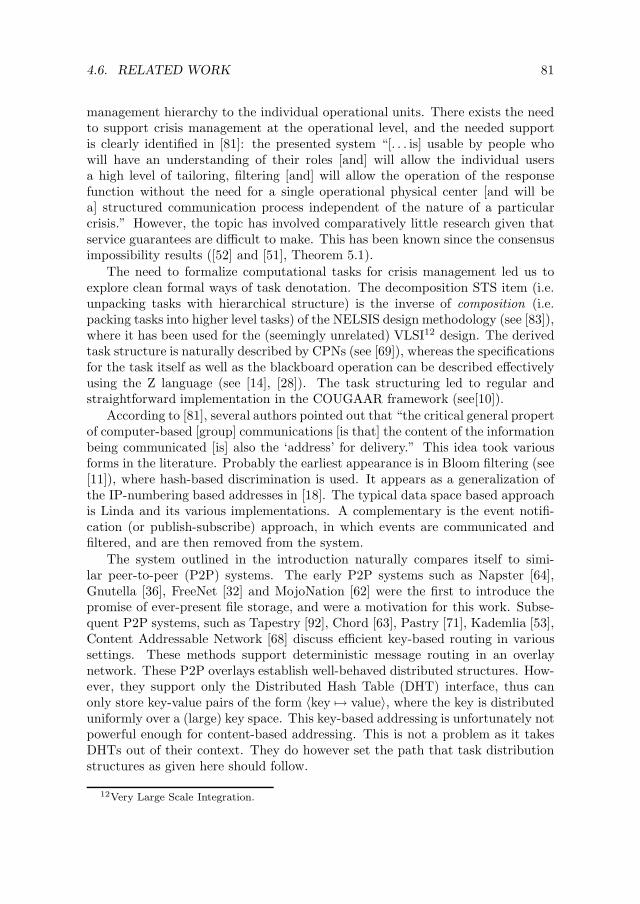
4.6. RELATED WORK 81
management hierarchy to the individual operational units. There exists the needto support crisis management at the operational level, and the needed supportis clearly identified in [81]: the presented system “[. . . is] usable by people whowill have an understanding of their roles [and] will allow the individual usersa high level of tailoring, filtering [and] will allow the operation of the responsefunction without the need for a single operational physical center [and will bea] structured communication process independent of the nature of a particularcrisis.” However, the topic has involved comparatively little research given thatservice guarantees are difficult to make. This has been known since the consensusimpossibility results ([52] and [51], Theorem 5.1).
The need to formalize computational tasks for crisis management led us toexplore clean formal ways of task denotation. The decomposition STS item (i.e.unpacking tasks with hierarchical structure) is the inverse of composition (i.e.packing tasks into higher level tasks) of the NELSIS design methodology (see [83]),where it has been used for the (seemingly unrelated) VLSI12 design. The derivedtask structure is naturally described by CPNs (see [69]), whereas the specificationsfor the task itself as well as the blackboard operation can be described effectivelyusing the Z language (see [14], [28]). The task structuring led to regular andstraightforward implementation in the COUGAAR framework (see[10]).
According to [81], several authors pointed out that “the critical general propertof computer-based [group] communications [is that] the content of the informationbeing communicated [is] also the ‘address’ for delivery.” This idea took variousforms in the literature. Probably the earliest appearance is in Bloom filtering (see[11]), where hash-based discrimination is used. It appears as a generalization ofthe IP-numbering based addresses in [18]. The typical data space based approachis Linda and its various implementations. A complementary is the event notifi-cation (or publish-subscribe) approach, in which events are communicated andfiltered, and are then removed from the system.
The system outlined in the introduction naturally compares itself to simi-lar peer-to-peer (P2P) systems. The early P2P systems such as Napster [64],Gnutella [36], FreeNet [32] and MojoNation [62] were the first to introduce thepromise of ever-present file storage, and were a motivation for this work. Subse-quent P2P systems, such as Tapestry [92], Chord [63], Pastry [71], Kademlia [53],Content Addressable Network [68] discuss efficient key-based routing in varioussettings. These methods support deterministic message routing in an overlaynetwork. These P2P overlays establish well-behaved distributed structures. How-ever, they support only the Distributed Hash Table (DHT) interface, thus canonly store key-value pairs of the form 〈key 7→ value〉, where the key is distributeduniformly over a (large) key space. This key-based addressing is unfortunately notpowerful enough for content-based addressing. This is not a problem as it takesDHTs out of their context. They do however set the path that task distributionstructures as given here should follow.
12Very Large Scale Integration.

82 CHAPTER 4. TASK MAPPING
Practical distributed systems often use indirection of system services to achievethe flexibility of the task mapping. In Section 2.3 of [79], two mechanisms forindirection are mentioned. First, “the agent requesting or providing a servicecommunicates with appropriate yellow pages server”. This line of design yieldssystems that are vulnerable to yellow pages server failures, an unwanted sideeffect. The second approach where “the agent requesting or providing a servicebroadcasts this fact to all appropriate agents”, admits the event notification anddata space approaches. The usefulness of event notification in dynamic networkshas been recognized (in [8]), and tree event distribution structures investigated (in[42]). A tuple-space implementation, albeit with disregard for efficient distributionis Lime (in [3]). We revisited the efficient distribution structures, and efficientactivation in [59] to show a set of approximate matching techniques (employed inan unrelated context in digital logic design in [23]) that simplify the distribution.
4.7 Summary
In this chapter we addressed the task mapping for DWEAM, a process that trans-forms the application requirements for a distributed system into a specificationthat can be implemented and subsequently executed by the DWEAM system.The specification is not a direct part of the DWEAM computer architecture, butdefines the DWEAM development environment. Given its fairly unconventionalnature when compared to mainstream object-oriented systems, it is important togive its detailed description.
We start from the task descriptions that we expect to be useful in emer-gency rescue operations. From there the generic task descriptions are extractedand refined, recognizing the Static Task Structure with task description and taskproperties. We then formalized the task structure. We described, proved anddemonstrated how the formalization fits into the executable CPN model, as aflexible executable structure admitting the task description. Thereafter, we de-scribe the mapping of tasks to nodes, via the CPN.
Then we present the design constraints, an important by-product of the im-mersion of a computer system into the real world. We point out the impossibil-ity results and give examples thereof, leading to probabilistic restatement of theproblem at hand. We then present the Distributed Blackboard used for the taskdistribution, and introduce the DB semantics by which the only allowed operationon the content is the addition. A consequence of such an access semantics is thatthe objects on the DB must be allowed to exist in multiple versions, and thatinsisting on object uniqueness in the traditional sense does not apply. Rather, weconclude that it must be allowed that multiple, possibly even conflicting viewsexist. We compare this approach by example to traditional distributed systems,where an unique fixed semantics is enforced.
A number of issues are deliberately left open in the exposition. We give ashort account of these issues here and explain how they are further dealt with.

4.7. SUMMARY 83
First, we give no argument that the task-level descriptions are adequate tocapture the crisis management tasks in full. Unfortunately, this is due to the factthat we have found the crisis management procedure descriptions to be ratherinformal, subject to positive regulations, and hence so far exclusively intendedfor human use. At the time of this writing, there is no formalized procedure thatcompiles these procedures into the structured task form that APL expects as in-put. The likely reason for the lacking description is that the use of informationsystems in crisis management is at its infancy and is still regarded as somewhatof an art rather than a codified discipline. This means that an adequate repre-sentation can be produced on demand, but that automated representation is stillnot feasible. The automated representation asks for independent research unre-lated to our main topic, and would require prohibitive resources. Thus, insteadof presenting the formalization we do the next best thing. We assume that sucha description can in principle be formulated, and offer a minimal interface fromthat description to the task structure we presented. This design decision allowedus to proceed with the design of the DWEAM system.
Second, the properties of the DM as introduced in Section 4.5 are temporarilyleft open. It is easily seen that the publish semantics that does not allow ob-ject removal must eventually exhaust the available memory at some nodes. Thisimportant issue is resolved in subsequent chapters. We will show that, althoughthe nodes are not able to control the memory they use for the object storageexplicitly, a form of garbage collection will guarantee timely reclaim of the un-used objects. In fact, we will show how the knowledge of the process structure,obtained through the data provided by the clients taking part in the DM helpsthe garbage collection. While the unbounded memory requirement is a valid crit-icism, there exist practical applications that work disregarding the unboundedmemory requirements. Example applications are the garbage collection mecha-nisms for the Java language (which allows the allocated memory to grow withoutbounds), and the version control systems such as CVS or Subversion (where therecords corresponding to versioned resources do not expire event if the resourcesthemselves are removed). The authors of practical applications thus have somefreedom to violate the rules of good conduct, when such violation can be justified.We too have used this freedom judiciously in our design of DWEAM.


Chapter 5
The Environment and StorageModel
The following Chapter describes the environment model assumed throughout thedesign of the DWEAM architecture. The environment model accounts for thenode and network volatility effects. Due to these effects, the availability of com-puting resources (i.e. the nodes and the network) changes over the system lifetime.Knowledge about the environment which is distilled in the appropriate model isused to understand how the adverse influence of the environment causing volatil-ity effects can be prevented. To this effect, in this Chapter, the basic propertiesof the environment model are presented.
5.1 Introduction
The DWEAM system consists of two distinct resource types: the nodes and thenetwork. The nodes abstract a collection of computers (PDAs, laptops and such),typically carried by their users, while the computing facilities are being exploited.This usage pattern is termed mobile user, to signify that the user changes physicallocation while using a service provided by own local computer. It is important tomake a distinction between the mobile and the nomadic user model. In the latter,the user only accesses the network infrastructure from various physical locations,but the mobility while the network is being used is negligible. This other usagescenario corresponds for instance with using the same laptop to access an Internet-based service both from home, and from work. The user carries the laptop fromhome to work and back, and uses it at both sites. However, the laptop is notbeing used in transit.
In the mobile user scenario each node has an attributed physical location. Thislocation may change over time, as the user changes its position. The networkresources at disposal in the mobile user scenario are typically radio-based. Theprevalent use case for the radio-based communication nowadays is that based on
85

86 CHAPTER 5. THE ENVIRONMENT AND STORAGE MODEL
GPRS, for which the existing communication infrastructure is used, such as thatof the mobile phone (e.g. GSM) networks. The GPRS usage scenario assumesthat a fixed communication infrastructure exists, and is terminated by the basestations. Each base station is used as a portal to the infrastructure for the usersthat are geographically close to that base station. Each user communicates onlyvia a base station to any other user on the communication network. This holdseven for users that are at a given time using the same base station for access (andare likely geographically close by).
In the DWEAM architecture, we consider an extended communication sce-nario, that drops the requirement for the existence of base stations, and a fixedcommunication infrastructure. Instead, the users need to cooperate in messagedelivery. Each user originally has a very limited view of the entire network, andcan directly contact only the nodes which are relatively geographically close. Thisis because of the path loss properties of the radio network. The network formedin this way is called a Mobile Ad-Hoc Network (MANET).
The MANET Properties
The MANET is induced by the time-variable graph of nodes and links, Gt . Theset of active nodes (active nodes(t)) at a given event time t depends on thenode availability that is induced by the environment. There typically exists aninterval of event times I == [t1 : Time, t2 : Time) during which a given nodex ∈ Nodes appears in active nodes(t), for some t ∈ I . thus any such node xcomes into existence at t1, and then lives on until it is permanently removed fromactive nodes at t2. Further, the existence of the connection in active links(t)depends in part of the position of the nodes through time. For each node inactive nodes(t), its position in a d -dimensional space is given as a function of realtime.
position : Nodes × real time 7→ Rd
∀(x : Nodes , τ : real time) •(x , τ) ∈ dom position ⇒ ∃ e ∈ Events •
RealTime(e) < τ ∧ x ∈ active nodes(e)
The goal of the MANET building is the establishment of a structure for com-munication between the network members. A lot of research is directed at under-standing the fundamental MANET properties. An account of MANET researchhas been given in [4]:
“Architectures have been primarily driven by a ‘point-to-point’ phi-losophy. We need to better understand a network viewpoint whereinnodes can cooperate intelligently taking advantage of the special prop-erties inherent in wireless communication.”

5.1. INTRODUCTION 87
“Architectures have been primarily centralized. We need to develophighly distributed architectures and algorithms that are still robustand energy-efficient on a system basis.”
[ . . . ]
“Research efforts have been primarily compartmentalized. We needhighly inter-disciplinary research across signal processing, communi-cations, game theory, and networking.”
To enable an integrated treatment of the MANET design issues, its relevantproperties are given in the list below.
1. Point-to-Point Connectivity. This property regards the density of the directconnections between the nodes in the network.
2. Connectedness and Structure. This property regards whether the MANETprovides connectivity so that any pair of nodes can connect either directly,or via multiple hops.
3. Capacity and Throughput. The capacity regards the maximum informationexchange rate that can be achieved in a given MANET under the idealtransmission schedule policy. The throughput regards the information ex-change rate that can be achieved under the adopted (likely suboptimal)transmission schedule policy.
4. Service Discovery. This property concerns the manner by which it is deter-mined which nodes need to communicate with each other, and communica-tion channels are established between them.
We now examine the MANET properties in more detail.
Point-to-Point Connectivity
The radio communication is based on the broadcasting of radio waves, at a certainpower level. With the increase in the physical distance, the power level of thesignal when it is received typically decays inversely proportionally to some powerof the distance. For a given transmission power level ρ, and a geographical distancer between the receiver and the transmitter, the received power level p is:
p =ρ
rα, (5.1)
where α is a path loss exponent. Typically, α = 2, although α can take onother values depending on the propagation model. We are interested in the largescale effect here, so will not elaborate on the possible values of α. The Signal-to-Noise-and-Interference Ratio (SINR) has two principal components: the ambientnoise, whose instantaneous power is assumed constant and denoted as N ; and

88 CHAPTER 5. THE ENVIRONMENT AND STORAGE MODEL
interference comprising of the signal powers of all the transmissions that areactive at a particular time instant. Given T , the set of all interfering nodes, Xt
for t ∈ T their positions, Xs the position of the sender and X the position of thereceiver, the SINR is given by:
SINR =ρ‖Xs −X ‖−α
N + ρ∑
t∈T
‖Xt −X ‖−α. (5.2)
The condition for the successful reception of a sent transmission from some nodes is that the resulting SINR is greater than some threshold β. The exact value ofβ depends on the adopted coding and modulation schemes, but regardless of theactual value of β, the general condition for successful reception of the form:
Esuccess ≡ SINR > β
is valid for many communication scenarios. The probability of an error a transmis-sion, the outage probability is the probability of the event E c
success, a complementof Esuccess from the equation above. It is usually required that for successfulcommunication it be bounded by prescribed level ǫ:
Pr (E csuccess) ≤ ǫ. (5.3)
Connectedness and Structure
Point-to-Point connectivity defines the conditions under which there can exist adirect connection between a sending and a receiving node. With the Point-to-Point as a basic element for connectivity, it is a logical followup to ask what isthen the resulting connection structure in Gt . In particular, it is important toknow under which conditions all nodes in Gt are connected, either by a direct link,or indirectly via a sequence of Point-to-Point links. The issue of connectednesshas been studied extensively in the continuum percolation theory (see Meesterand Roy [54]), from which our model for the connectivity is adopted. Here thepercolation model for the connectivity concerns the structure of position(x , τ) forany node x and a given real time stamp τ .
We model the node positions by a stationary point process (see Meester andRoy, [54], page 9). That is, we assume that each node has a randomly chosenposition in the space R
d . The dimension d can be an arbitrary positive integer.Being application driven, we only consider the case d = 2, yielding a node config-uration on a two-dimensional surface (e.g. plane). To make the notion of a pointprocess more precise, one considers the set R
d , and the σ-algebra of Borel setsin R
d as Bd . Denote by N the set of all counting measures on Bd for which themeasure of a point is at most 1. Equip N with a σ-algebra N generated by thesets of the form:
n ∈ N • n(A) = k

5.1. INTRODUCTION 89
where A ∈ Bd , and k an integer.
A point process X is a measurable mapping from a probability space (Ω,F ,P)into (N ,N ).
The definition of N allows one to count the number of points in a set A ∈ Bd .In words, X (A) represents a random number of points inside A. A point processX is stationary, if its distribution P is invariant under an arbitrary translation.
The point process X is said to be a Poisson process with density ξ > 0 if thefollowing are satisfied:
1. For mutually disjoint sets A1, A2, . . . , Ak the random variables X (A1) . . .X (Ak)are mutually independent.
2. For any bounded set A ∈ Bd , we have for each k ≥ 0:
Pr (X (A) = k) = e−ξ‖A‖ [−ξ‖A‖]kk !
, (5.4)
where ‖A‖ is the measure of the area A. The parameter ξ is the density of thecorresponding Poisson process.
For the node connectivity, the description of a Poisson point process is am-mended. Following Meester and Roy, a Poisson Random Connection Model(RCM) is set up. The RCM describes the connection structure in a d -dimensionalspace induced by a non-homogeneous Poisson process. Again d = 2 is assumed.For Ai ⊆ R
d (d ∈ N ), a random process X is a non-homogeneous Poisson processwith density ξ > 0 if the following properties are satisfied:
1. For mutually disjoint sets A1, A2, . . . , Ak are mutually independent.
2. For any bounded set A ∈ Bd , we have for each k ≥ 0:
Pr (X (A) = k) = e−ξ∫
Rdg(x)dx
[−ξ∫
Rd g(x )dx]k
k !. (5.5)
The function g : Rd → [0, 1] is the intensity function. For our purposes, g is
the distance-based connectivity between the nodes. We assume a static model inwhich the following holds, with r and q vectors in R
d :
• g(r) = g(q) whenever ‖r‖ = ‖q‖,
• g(r) ≤ g(q) whenever ‖r‖ ≥ ‖q‖.
The derivation for g(r) for the MANET is given further in the text.

90 CHAPTER 5. THE ENVIRONMENT AND STORAGE MODEL
Capacity and Throughput
MANETs are formed by mobile computing devices equipped with radio antennasthat are used to communicate. Usually the range for the successful communica-tion is limited, so communication between distant nodes is only possible if nodescooperate by relaying messages to each other. In [39], Kumar and Gupta assumedan optimal routing scheme to discover the throughput capacity of an arbitraryMANET of n devices, with an available radio channel of capacity W bits persecond, in an unit area is of the form Θ(W /
√n log n). Their analysis is based on
the following assumptions:
1. The traffic patterns in the MANET are random. Pairs of devices, one trans-mitter and one receiver, are chosen independently at random and packetsare sent between them.
2. The packet routing is optimal. The packets are delivered along the shortestpath between the transmitter and the receiver.
Under the transmission models given in [39], these two assumptions lead to theachievable throughput of an arbitrary MANET. The achievable throughput asderived in the said paper is, in fact, the raw throughput. It is unreasonable toassume that it reflects the useful throughput too. This is because the analysisis conditioned on the assumed known traffic pattern. The sender and receiverpair groups are assumed pre-determined by an unspecified device that has beenabstracted away of the analysis for simplicity reasons. In real-life applications itis necessary to determine the traffic pattern before any of the wireless connectionscan be used. This is named service discovery.
5.2 Connectivity Function
In this section, we derive the analytical form of g(r), the connectivity functionof the RCM in the MANET case. Consider a receiver placed on a planar sur-face. Assume that its position determines the coordinate origin of an appropriatecoordinate system. To derive g(r) one needs to find the probability that, underthe transmission model of the equation (5.3), a transmission from a transmitterat distance r from the origin is successfully received. The interference is due tothe ambient noise, assumed to be time-invariant and with mean power equal toN , and the signals produced by the transmitters that operate independently butconcurrently to the considered transmitter.
Exact Analysis
For successful transmission, for all the nodes transmitting simultaneously, equa-tion (5.2) must hold. Consider a circle C with the radius R on the planar surface.
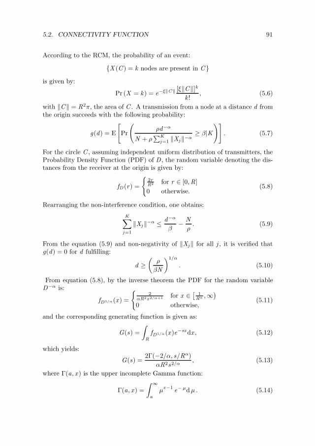
5.2. CONNECTIVITY FUNCTION 91
According to the RCM, the probability of an event:
X (C ) = k nodes are present in C
is given by:
Pr (X = k) = e−ξ‖C‖ [ξ‖C‖]kk !
, (5.6)
with ‖C‖ = R2π, the area of C . A transmission from a node at a distance d fromthe origin succeeds with the following probability:
g(d) = E
[Pr
(ρd−α
N + ρ∑K
j=1 ‖Xj‖−α≥ β|K
)]. (5.7)
For the circle C , assuming independent uniform distribution of transmitters, theProbability Density Function (PDF) of D , the random variable denoting the dis-tances from the receiver at the origin is given by:
fD (r) =
2rR2 for r ∈ [0,R]
0 otherwise.(5.8)
Rearranging the non-interference condition, one obtains:
K∑
j=1
‖Xj ‖−α ≤ d−α
β− N
ρ. (5.9)
From the equation (5.9) and non-negativity of ‖Xj‖ for all j , it is verified thatg(d) = 0 for d fulfilling:
d ≥(
ρ
βN
)1/α
. (5.10)
From equation (5.8), by the inverse theorem the PDF for the random variableD−α is:
fD1/α(x ) =
2
αR2x2/α+1 for x ∈[
1Rα ,∞
)
0 otherwise,(5.11)
and the corresponding generating function is given as:
G(s) =
∫
R
fD1/α(x )e−sxdx , (5.12)
which yields:
G(s) =2Γ(−2/α, s/Rα)
αR2s2/α, (5.13)
where Γ(a, x ) is the upper incomplete Gamma function:
Γ(a, x ) =
∫ ∞
a
µx−1
e−µd µ . (5.14)

92 CHAPTER 5. THE ENVIRONMENT AND STORAGE MODEL
A sum of K random variables as in equation (5.9) has the generating functionGK (s). The corresponding PDF is then given by:
f (x ) =1
2πi
∮
M
GK (s)esxds . (5.15)
The equation (5.15) is, however, unlikely to yield a useful result, as G(s) cannotbe further simplified. We leave the Equation (5.15) at that, and resort to findingan approximate solution to the problem.
Approximate Solution
Resorting to an approximate solution, assume that K is large with high proba-bility. For large K , the equation (5.7) yields itself to Gaussian approximation.However, we will not approximate all the transmitters with a Gaussian distribu-tion. Looking at Equation (5.1), it is seen that the interference from the far-awaynodes must be low, as it decays fast with the distance. Also, the expected num-ber of such nodes is high, as the expectation of Equation (5.4) is proportional tothe size of the considered area. Hence for this area the Gaussian approximationis justified. The transmitters are therefore split into two groups: the near andthe far group (Figure 5.1). The near group consists of the transmitters between
r2Near group
Far group
r1
Figure 5.1: The near-far group approximation for computing the connectivityfunction g(d).
0 and r1. The far group consists of the transmitters between r1 and r2, where0 < r1 ≤ r2 →∞.
The first limit, r1 is the critical radius (also denoted further on as rc), desig-nating an area within which any single interfering transmitter completely prevents

5.2. CONNECTIVITY FUNCTION 93
the message communication with the receiver at the origin. The second limit, r2in principle can be set arbitrarily far away, and further in the text we assumer2 →∞.
Theorem 2 (Critical radius) Consider the planar arrangement of nodes, witha receiver placed at the coordinate origin. Also consider a transmitter, at distanced, with the path loss exponent α > 2. The critical radius rc is given as:
rc =d−α
β− N
ρ(5.16)
Proof. Consider the non-interference model, as given in the Equation (5.2).Assume that there is only one interfering node, i.e. #T = 1 at distance r fromthe receiver. Assume the receiver and the transmitter are at a distance d . Then:
SINR =ρd−α
N + ρr−α . (5.17)
From the receive condition SINR ≥ β, substituting the expression for SINR fromEquation 5.17, and introducing renaming [rc/r ], one obtains the claim.
Considering that the critical radius rc is non-negative, one can again obtain thelimiting condition for d for any connectivity to exist. Observing that rc ≥ 0 andusing Equation 5.16, one obtains the same condition as was given in Equation 5.10.
Function g(d) is in effect the probability of the connection existence given thedistance between the receiver and the transmitter. The following proposition isnaturally derived from this assumption.
Proposition 1 (Disk Connectivity) Let g(d) be the probability of the connec-tion existence. Then the connectivity in the sense of Equation (5.3) is:
Pr (Esuccess) = [g(d) > ǫ] (5.18)
where [·] is the Iverson (indicator) function [37].
From the proposition 1 it is seen that the area (with respect to d) has the shape ofa disk, provided that g(0) > ǫ, as g is monotonic and non-decreasing, as requiredby the model given in the Section 5.1. We will now give an expression for g(d).
For this purpose, we divide the planar area outside of C into concentric,infinitely thin annuli. As in the Section 5.2 it can be seen that trying to accountthe exact contribution of all of the interferers leads to expressions which areimpractical to evaluate (the connectivity expressed through the upper incompleteGamma function), the only resort is to try a suitable approximation.
We attack this problem using the common balls-and-bins approach, as follows.Consider the annuli into which the R
2\C is divided as “bins”, each carrying somenumber of “balls”, each “ball” being an interferer node, which happens to belocated at this particular bin. Let X (r) be the interference contribution for the

94 CHAPTER 5. THE ENVIRONMENT AND STORAGE MODEL
annulus (“bin”) dC at the distance r from the origin, and dr thick, with dr → 0.The probability dPr (n(dC ) = k) that there are k interferers in this area is:
d Pr (n(dC ) = k) =∂
∂r
[e−ξr2π (ξr2π)k
k !
]dr . (5.19)
for k ∈ N0, and the contribution of each bin is then:
dX (r)r−α (5.20)
where dX (r) is a random variable with the distribution given in Equation (5.19).The total interference is then given as:
Y =
∫ ∞
rc
r−αdX (r). (5.21)
While it is still involved to compute the distribution of the cumulative interferenceY exactly, given that it is the sum of independent random variables, the Gaussianapproximation may be invoked. For this, E [Y ] and Var [Y ] must be computed.The variable Z = (Y − E [Y ])/
√Var [Y ] is then the Gaussian-distributed unit
variance, zero mean random variable. An elementary lemma helps to obtain E [Y ]and Var [Y ]:
Lemma 1 For a random variable V =∑
i Vi , of independent random variablesVi , the following holds:
E [V ] =∑
i
E [Vi ]
Var [V ] =∑
i
Var [Vi ] .(5.22)
Using Lemma 1, the moments for Y are obtained.
Proposition 2 Let Y be a random variable, defined as in Equation 5.21. Then,E [Y ] and Var [Y ] are given as:
E [Y ] =2ξπ
α− 2r2−αc
Var [Y ] =4ξ2π2
2α− 3r3−2αc − (E [Y ])2.
(5.23)
where α > 2.
Proof. By Equation 5.21, we have:
E [Y ] =
∫ ∞
rc
2ξrπr−αdr =2ξπ
α− 2r2−αc , (5.24)

5.2. CONNECTIVITY FUNCTION 95
conditioned on α > 2. Similarly, for E[Y 2], one obtains:
E[Y 2]
=
∫ ∞
rc
4ξ2r2π2r−2αdr =4ξ2π2
2α− 3r3−2αc (5.25)
conditioned α > 3/2. Together with the condition of Equation 5.24, it amountsto α > 2.
By central limit theorem:
Proposition 3 The random variable Z = Y−E[Y ]√Var[Y ]
has Gaussian PDF with zero
mean and unit variance, where E [Y ] and Var [Y ] are found in Proposition 2.
The successful reception condition in Equation 5.7 (i.e. the conditional thereof)is rewritten in terms of Z to be:
g(d | n(C ) = 0) = Pr
(Z ≥ d−α/β − ρ/P − E [Y ]√
Var [Y ]
), (5.26)
which is then given in terms of the function Φ(z ) = (2π)−1/2∫ z
−∞ exp(−z 2/2)dz )to be:
g(d | n(C ) = 0) = 1− Φ(d−α/β − ρ/P − E [Y ]√
Var [Y ]), (5.27)
for d constrained in the sense of the Equation (5.10).We have therefore proven the following:
Theorem 3 The connectivity function g(d) is given by:
g(d) =
[1− Φ(
d−α/β − ρ/P − E [Y ]√Var [Y ]
)
]e−ξr2
c π, (5.28)
with all the quantities appearing in Equation 5.28 as defined previously in the text.
Thus, starting from the basic assumption about the distribution of the nodes,stemming from the RCM model, we derived the approximate condition for thefunction g(d), denoting the probability of successful reception (hence: the exis-tence of a connection) between a transmitter and a receiver at a distance d , in thepresence of an unbounded number of interferers, distributed uniformly at randomin R
2.The range function depends on g(d) as: [g(d) > ǫ], where ǫ is a parameter
depending on the techniques used to modulate the transmitted signal. As g(d) ismonotonically non-increasing, the shape of the successful reception area is alwaysa disk. However, independent of the modulation technique, there is a criticalradius rc , for which all transmission necessarily stops. This critical radius is dueto the existence of the “background” noise that slowly but surely drowns thesignal, as the distance between the transmitter and the receiver increases. In this

96 CHAPTER 5. THE ENVIRONMENT AND STORAGE MODEL
Chapter, both the upper bound g(d) and the Gaussian approximate for g(d) arecomputed in terms of the system parameters.
The implication for the connectivity structure is strong. The connectivityg(d) imposes a limit to the number of nodes that can be contacted by any givennode. Moreover, the nodes are within a limited radius. This implies that a datastructure that requires “far reaching” connections can not be implemented withconstant resources per node. This because for a node to reach a distant receiverit must use a number of intermediate nodes proportional to the distance betweenit and the destination, divided by at least the maximum range. A node mustconsider the soft state recorded by all the intermediate nodes, and this cannotever be made to be significantly less than the stretch of the graph.
5.3 The Storage Model
In this section, we turn the attention to the reliability of storing data to nodesin a volatile network. We present an analysis of using the fragmentation of datainto tags, and depositing the tags onto various nodes in a multi-agent network,to achieve resilience against node volatility. We emphasize Multi-Agent Systems(MASs) as example platforms in which there is system-wide interest in preservingdata. Agent programs in a MAS often use an agent platform as middleware [50].The platform controls the messaging and the agent life-cycle. The reliability ofthe agent platform has received little attention in practice, though it is recognizedas a MAS issue [80].
Notable MASs, such as JADE [85] or COUGAAR [10], assume a reliable plat-form. Sometimes the platforms provide persistence to non-volatile media, pro-tecting the agents from transient failures. For both platforms, replication servicesexist; these services have been implemented with simplicity in mind, rather thanefficiency. We use information-theoretic arguments to show how efficient reliabil-ity in a MAS can be derived from cooperation with a slight trade-off for increasedcomplexity. The resulting platform is called Combined [1]; this platform is basedon the COUGAAR agent architecture, with additions that make it suitable fordeployment in chaotic, rapidly changing environments.
Application
The main motivation for looking at increasing the reliability of multi-agent plat-forms is because it is desirable in applications. We will mention two applicationswhich benefit from the Combined approach.
Emergency search-and-rescue operations benefit from timely information de-livery. This deployment setting was also adopted as the prototype application forCombined. We envision a near-future application in which members of emergencyservice units (police, fire brigade, ambulance etc.) are equipped with short rangecommunication devices. Due to the nature of the deployment, it cannot assume

5.3. THE STORAGE MODEL 97
that communication infrastructure exists; the reliability of the communicationdevices can also not be taken for granted. The devices work around these imped-iments by cooperating in message delivery and keeping each other’s observations;the body of the Chapter explains the theory on which this possibility is based.
Large scale distributed scientific applications, such as Seti@Home [74], or Fold-ing@Home [31] succeeded in harnessing worldwide processing power for highly de-manding computational tasks. The focus of their system architectures has shiftedfrom traditional parallel and distributed computing efficiency issues [51] to or-ganizing and managing redundant work done by worldwide computers. Someindication of the system architecture can be found at [13]. The Combined ap-proach might aid this effort by offering a way to preserve computation resultsdespite computers leaving the network.
Related Work
The system outlined in the introduction naturally compares itself to similar peer-to-peer (P2P) systems. The early P2P systems such as Napster [64], Gnutella [36],FreeNet [32] and MojoNation [62] were the first to introduce the promise of ever-present file storage, and were a motivation for this work. Subsequent P2P systems,such as Tapestry [92], Chord [63], Pastry [71], Kademlia [53], Content AddressableNetwork [68] discuss efficient key-based routing in various settings. These meth-ods support deterministic message routing in an overlay network. OceanStore [46]is an architecture for establishing global persistent storage; similarly, the Coop-erative Filesystem (CFS) is an application that uses Chord to make a P2P-basedread only storage system. Unlike Combined, all these systems work with an over-lay on top of an existing Internet Protocol (IP). The underlying IP network layerallows cheap contact between any pair of the participants. The interconnect meshcorresponds to a complete graph. However, Combined is established on a spatialproximity based network mesh, with connections induced by the distance betweennodes. Due to this external constraint, the interconnect mesh is much sparserthan that of the mentioned systems. The contact between far away nodes can becostly. Typically, the transitive closure of the Combined interconnect mesh wouldcorrespond to the IP-based interconnect used by the mentioned P2P systems. An-other important distinctions is that in Combined, cooperation is needed for eventhe simplest operations such as contacting a far away node. In the mentionedP2P systems, this operation is handled by a lower level network protocol. Thelayering simplifies the design, but limits the applicability of the overlay to net-works in which IP is efficient. The ideas of Combined are most thoroughly sharedwith OceanStore. This architecture uses erasure coding to achieve high data reli-ability. The improvement from using erasure coding over replication was clearlyshown in another paper [87] from the co-authors of OceanStore. OceanStore con-siders erasure coding only for deep archival; but also goes to considerable lengthto handle data security. Combined intends to use data archival to provide processpersistence; but it does not consider data security explicitly. This difference is

98 CHAPTER 5. THE ENVIRONMENT AND STORAGE MODEL
easily understood in the light of the Combined prototype application. In such asetting, it is reasonable to assume that cooperative behaviour by far outweighscompetitive or malevolent behaviour.
Result
We present a graph-theoretic model using erasure graph to describe the systeminterconnect and evolution, and partition encoding for allocating data pieces (tags)to different agents in Section 5.4. We then use this model to derive the storagecapacity of the resulting society, and prove that the capacity cannot be largerthan the availability figure of the most reliable agent in the network (Section 5.4).Assuming the availabilities are known, we describe the strategy that an agentcan use to determine which code and data partition to choose to make best useof the available capacity (Section 5.4). We first give a calculation for a generalinterconnection case, and random agent position within the network. We thensimplify the analysis by layering the neighbours in tiers and allowing agents todelegate pieces of work to each other.
5.4 System Model
We now give an overview of the system setup and notation. For detailed def-initions and more flexible models, the reader is referred to [56]. The networkof nodes is constructed based on the interconnections created by a short rangeradio network: two nodes are connected if they are closer to each other than apre-determined range. This is a reasonable assumption, shared by papers closelydealing with wireless network properties, such as [39]. Denote as V the set ofnodes v1, . . . , vm. If a connection between two different nodes vi and vj exists,we insert the pair vi , vj into the set E . The graph G (V ,E ) is interpreted in theusual sense: V is a set of vertices, and E is a set of corresponding edges. Whenwe need to emphasize that V or E belong to a graph G, we write VG and EG ,respectively. The interconnection mesh of G changes as the nodes move, join orleave the network. When nodes leave the network, it can happen either voluntarilyor involuntarily; the latter can occur because of network partitions or nodes beingdamaged, out of power, or destroyed. The involuntary leave is called an erasure.Due to nodes leaving the network, the interconnection graph degrades. If a nodev leaves, it is removed from V , along with the corresponding edges from E . Herewe assume that each node can leave independently with identical probability ε.We call the graph G the erasure graph.
Consider a source node v from V that has during its lifetime produced valuabledata (a tag) that should be preserved in case that v gets erased. Node v can chooseto deposit copies of the tag with its neighbours. Depositing copies is commonlycalled replication. This approach, although effective, uses too much excess storage.Moving tags also spends bandwidth and a smart source node would want tominimize the spending. In [87], an alternative approach was discussed, whereby

5.4. SYSTEM MODEL 99
the node uses an erasure code to transform the tag and deposits only fragments ofthe resulting coded messages to neighbours. Thanks to the coding, only a fractionof the fragments is required for successful decoding. There exist efficient methods(for instance, the iterative decoding method from [70]) to recover original tags.OceanStore and CFS [22] use these methods, but assume that the missing tagswere erased independently, and those that remain are accessible independently. Inthe locally-connected network mesh, these assumptions do not necessarily hold.When trying to deposit a tag, v will have a choice of contracting several neighboursand request them to be tag keepers. Typically, v will want to pre-code the tag assaid before copying to the keepers. v would then make a partition of the entiremessage. The partition is described by a set Π = π1, . . . , πm. Each elementof the partition is in itself a set denoting which bit of the encoded message isallocated to which node. For example, if the message was 5 bits long, and 2 nodeswere available, one possible partition would be: Π = π1, π2, where π1 = 1, 2and π2 = 3, 4, 5. This means that bits 1 and 2 are allocated to the node withindex 1, and bits 3, 4 and 5 are allocated to the node with index 2.
To store the fragments, the source node v chooses the code and the parti-tion. It then contacts the nodes, as defined by the partition, and deposits themessage fragments. This is called a write. To retrieve the stored information, vcontacts all the available keepers and retrieves the fragments. The fragments arethen re-assembled and decoded to produce the original tag. This is called a read.Between the writes and corresponding reads, the keepers may be erased, or maybe unavailable at the time of the read. Although each keeper has a probability εto disappear, its availability also depends on its connection to other nodes. Wewill denote the availability of the node vi from V as wi . The writer will typicallywant to know in advance the availability of the potential keepers to decide whichpartition is the “best”. Due to erasures, the graph G could be partitioned intoconnected components. We denote as QG the set of all maximal connected com-ponents for a given graph G. These maximal connected components are calledchains. Two simple writer decisions are given in the following examples. The de-cisions are named according to the cooperation policy: the Lone Ranger prefersto keep all the message to itself; the Cloner prefers to make multiple identicalcopies of the message.
Example 9 (The Lone Ranger) The source decides to keep the entire messageon a single node. The probability that the message is readable is: Pr (readable) =Pr (keeper alive) · Pr (path to keeper exists) ≤ Pr (keeper alive) = ε.
While the total storage is minimized, any transition that erases this singlekeeper destroys the tag.
Example 10 (The Cloner) The source node decides to duplicate the tag withk keepers. This ensures that if at least one keeper is present, the entire tag can beretrieved. However, the case in which such storage space investment is justifiedis very improbable. The probability that all but one keeper are absent is: k(1 −ε)εk−1 ≤ kεk−1, and tends exponentially fast to zero with k.

100 CHAPTER 5. THE ENVIRONMENT AND STORAGE MODEL
While the data cannot be protected better, the frequency of the catastrophicevent is too low for the storage spending to be justified.
The Capacity of the Erasure Graph
Let there be given a connected graph G. For the given graph G, a writer wouldlike to know the storage capacity that G can offer. This section provides tools todo just that. Let us denote as X the message that a writer needs to distributeacross the network formed by nodes V . For convenience, we consider that Xis a string of n binary digits (bits). As in practice all data objects used in acomputer system can be represented in this way1, we only need to consider thebinary strings further in the text.
Each bit of the message X should be stored to some node in G. As the nodesin G are volatile, it is to be expected that not all the bits from X can be recoveredonce they are handed out to nodes in G. From that perspective, G behaves as alossy erasure channel: the writer stores data expressed as bit-strings into it andthe reader retrieves a damaged bit string, with some bits irreversibly lost due tothe volatility of the nodes that stored them. The reader will be able to retrieveonly some fragments of the original message (call the fragments Y ), due to thedegradation of the network. We will consider each bit of X as a channel use
The mutual information2 on X and Y is given as: I (X ,Y ) = H (X ) −H (X |Y ), where H (X ) and H (X |Y ) are, in order, the entropy of a randomvariable X and the conditional entropy of a random variable X given Y [21].
Since when X is known, then any Y is known, it holds that: I (X ,Y ) =H (Y ) − H (Y |X ) = H (Y ), i.e., knowing X gives all the information over Y .The writer has some freedom to choose the partition Π, if it knows the availabilities(written as: wi) for the nodes vi from V .
This way, H (X |Y ) becomes a function of Π. Knowing all wi , writer can choosethe Π that maximizes H (X |Y ). The capacity of G is then C = maxΠ I (X ,Y ).We now express C in terms of wi in Theorem 4, and find C explicitly in Theorem 5.
Theorem 4 (The Capacity of G given Π) Let G be an erasure graph. Thecapacity of the channel defined on the graph G, under a given partition encodingΠ and assuming uniform connection probability, is obtained by solving a linearprogram:
C = maxΠ
∑
1≤i≤#V
wi#πi ;∑
1≤i≤#V
#πi = n, (5.29)
1Encoding objects for transfer into binary strings explicitly is common practice. Facilitiesto achieve this are present in many programming languages, and libraries where the feature isnot provided by the language.
2The meaning of mutual information in this case is simply the number of bits shared by Xand Y . Likewise, the entropy H (X ) is the number of bits in X , and the conditional entropyH (X |Y ) is the number of bits that are left unknown in X if we know all the bits of Y .

5.4. SYSTEM MODEL 101
where coefficients wi for 1 ≤ i ≤ #V depend on the connectivity of the graph G:
wi =
#V−1∑
e=0
εe(1− ε)#V−e
#V − e·
∑
Ep∈Pe
∑
H∈QEpG
#VH [vi ∈ VH ] .(5.30)
In Equation (5.30), Ep is the erasure pattern, a function mapping each vertex ofG into the set 0, 1 and associated with a particular transition. It maps v ∈ Vto 1 if v is erased by the transition, or to 0 if v is not erased by the transition.Ep can be applied to QG , to obtain a new connected components set: each vertexthat Ep maps to 1 is removed from G along with corresponding edges. QEpG arethe connected components that G is split into, after applying the erasure patternEp . Pe is the set of all erasure patterns on G, having exactly e erasures. Aconsequence of Theorem 4 is the maximum capacity obtainable for a given graphG.
Proof. The probability of e erasures on a single transition is given by:
Pr (e erasures) =
(#V
e
)εe(1− ε)#V−e .
Generate the set of all possible erasure patterns for a given e and name it Pe .Every Ep ∈ Pe induces a set of connected components QEpG , and each of thesets is composed by connected graphs GEi ∈ QEpG . The mutual informationI (X ,Y ) is the mean of the number of bits retrieved from all the possible erasurepatterns. The set of all possible erasure patterns P is given by the union ofall individual erasure patterns: P =
⋃0≤e≤#V Pe . The average number of bits
retrievable from the channel depends on the particular transition, and ultimatelyof the erasure pattern within. Considering e known and looking at a particularerasure pattern Ep , the average number of bits is obtained by averaging over allpossible connection points, since by assumption of the theorem, a reader can bewith uniform probability connected to either of the remaining nodes of G.
I(X ,Y |QEpG
)=
∑G∈QEpG
#VGI (X ,VG)∑
G∈QEpG#VG
. (5.31)
From here it is easy to obtain that:
I (X ,Y ) = E[I(X ,Y |QEpG
)](5.32)
will yield the expression for mutual information for X and Y . These expres-sions depend upon elements of Π. The expression in Equation (5.32) includesmulti-dimensional sums, which ultimately depend on the (beforehand unknown)

102 CHAPTER 5. THE ENVIRONMENT AND STORAGE MODEL
connectivity of graph G. Let e remain fixed, and let us focus on Equation (5.31).For a given v ∈ V , define 〈v〉 to be the index of v . Substituting I (X ,VG) by:
∑
v∈VG
#π〈v〉,
it is seen that #π〈v〉 enters the sum on a number of occasions.It is possible to determine how many times and with what weight coefficient
does #π〈v〉 appear in the appropriate equation, and the answer depends on e andon the size and number of the connected components that v can belong to. Letthe connected components be named chains, for convenience. The shortest chainthat v can be part of has size 1, when v is its only element. The longest chainhas size #V , when no degradation takes place. If v belongs to a chain of size l ,when e errors are present, its contribution to expression (5.32) depends on theposition of v in the string.
There are different ways in which v can be a member of a chain of size l .Expanding the expectation in Equation (5.32), one obtains
I (X ,Y ) =E[I(X ,Y |QEpG
)]
=∑
Ep∈P
∑G∈QEpG
#VGI (X ,VG)∑
G∈QEpG#VG
Pr(QEpG
),
(5.33)
and averaging the number of bits retrieved from each element of P will giveI (X ,Y ). Since the degradation model is i.i.d., the probability of each Ep ∈ Pe
is equal to εe(1 − ε)#V−e . By introducing an indicator function it is possible torestate I (X ,VG) as:
I (X ,VG) =∑
v∈VG
I (X , v)
=
#V∑
i=1
I (X , vi) [vi ∈ VG ]
=
#V∑
i=1
#πi [vi ∈ VG ] , (5.34)
permitting the separation of the sum in Equation (5.31) as:
I (X ,Y ) =∑
Ep∈P
Pr(QEpG
)∑
G∈QEpG#VG
·
·∑
G∈QEpG
#VG
#V∑
i=1
#πi [vi ∈ VG ] .
(5.35)

5.4. SYSTEM MODEL 103
Substituting P , Equation (5.35) becomes:
I (X ,Y ) =∑
Ep∈⋃
0≤e≤#VPe
εe(1− ε)#V−e
∑G∈QEpG
#VG
·
·∑
G∈QEpG
#VG
#V∑
i=1
#πi [vi ∈ VG ] .
(5.36)
When Ep is an element of Pe , then the following expression holds:
∑
G∈QEpG
#VG = #V − e, (5.37)
which is easily seen to be true, as∑
G∈QEpG#VG is the total number of nodes
present in the connected component QEpG .By changing the order of summation in Equation (5.33) such that the first sum
goes over all πi , and noting that for e = #V the sum component is equal to zero,one is able to find: I (X ,Y ) =
∑#V
i=1 wi#πi , where wi is given by Equation (5.30).
Theorem 5 (The Capacity of G) Let the channel be defined on the graph G,and let all availabilities wi be known for all nodes vi from V . Let:
w∗ = max 1≤i≤#V wi .
Then: C = nw∗.
This is to say that, regardless of the choice of the partition Π, it is not possible toobtain the rate (ratio C/n) greater than the maximal availability of all the nodesin G.Proof. Let wi and πi be permuted, without loss of generality, so that w∗ =w1 ≥ w2 ≥ · · · ≥ w#V .
C = maxΠ
∑
1≤i≤#V
wi#πi ≤ w1
∑
1≤i≤#V
#πi = w1n, (5.38)
since for each i , wi#πi ≤ w1#π1.
The Choice of the Partition
We have seen how the node availabilities affect the storage capacity achievable bya given graph G. We will now describe the strategy the writer uses to find the“best” partition. In [56], the subset of acceptable partitions is captured by thenotion of distortion in the following definition.

104 CHAPTER 5. THE ENVIRONMENT AND STORAGE MODEL
Definition 8 (Distortion) Consider some erasure graph G. Let QG be the setof connected components of G, and let the partition Π be known for distributinga message X over nodes in V of G. The distortion of some QG (written as:d(QG)) equals to the expected tally of irretrievable message bits of X , over allpossible erasure patterns.
Thus, the distortion tells us for the connected components QG of some graphG, how many bits are expected to be be lost, when the graph undergoes anarbitrary erasure pattern.
Proposition 4 (Distortion Properties) Consider the distortion as given inthe Definition 8. Consider some transition between the components QG andQEpG . Denote as Dc be the set of all possible connected component configu-rations obtainable by applying an erasure pattern Ep to QG, and let V (QEpG)be the set of all vertices thereof.
1. Let R = (1− εT )n −∑i∈V (QEpG) #πi . Then the distortion. Then:
d(QG) =∑
QEpG∈Dc
Pr (Ep) · R · [R > 0] . (5.39)
2. Let πi be the partitions for nodes vi . d(QG) is a non-negative piecewiselinear function of #πi .
Proof. The property 1 is immediate. For property 2, note that every termof Equation 5.39 is non-negative. All #πi are non-negative. Setting all πi to beempty sets (corresponding to maximum distortion), the maximum of d(QG) isgiven by:
d(QG) = (1− εT )∑
QEpG∈Dc
Pr (Ep) · [(1− εT )n > 0] = (1− εT )n. (5.40)
By re-expressing d(QG) in terms of #πi , we get:
d(QG) = a0,C −∑
i
ai,C#πi , (5.41)
where a0,C = (1 − εT )n, and ai,C 6= 0 in general.
Given a maximum distortion dmax and the area
v(dmax) = QEpG | d(QEpG) ≤ dmax,the best configuration Q∗
G is given by
Q∗G = arg minQ∈v(dmax) f (Q), (5.42)
where f is a disambiguation function that helps in the choice of the unique solu-tion. The parameter εT is the decoding threshold [70] of the employed decoder,the fraction of n that can be erased, without entailing decoding error. f is a goalfunction picked according to design criteria:

5.4. SYSTEM MODEL 105
1. Given a threshold εT , decoding must succeed if erasure fraction is less;
2. Given two partitions from v(dmax), the encoder chooses a “more distributed”one;
3. The encoder must handle a variable number of hosts (#V ), and variablemessage lengths n.
The requirement 1 is implicitly satisfied by choosing a threshold-εT code.Further requirements can be satisfied in different ways. We choose the partitionΠ such that the sum-squared of all fragment lengths (ni = #πi) is minimal. Thechoice amounts to using:
f (C) =
(∑
i
(#πi )2
)1/2
, (5.43)
effectively choosing as the configuration to be at the the point closest to theall-zero configuration, i.e. the one where all bits on all nodes were lost.
This choice is akin to mean-square energy minimization in multi-channel signaldetection: we assume that each fragment length contributes independently tothe entire tag. The expected number of retrieved bits must be equal to (1−εT )n.This expression is precisely equal to the sum of ni weighed by wi for each node.Finally, the fragments should form a partition of the message, thus the sum of ni
must be equal to n. For the same reason, for all i , the condition ni ≥ 0 must hold.The distortion corresponds to the distance (in the number of lost bits) between
v0
v1 v2
v3
Figure 5.2: Subdividing V into subsets headed by nearest neighbours. v0 is thewriter. It delegates 3 fragments of a single tag to its nearest neighbours, v1, v2,and v3. v0 also delivers ζ1 and ζ2 to each of the neighbours so that they would beable to further sub-divide their fragment.
the complete message X and any received message Y . An example contour plotof d(QG) for a two-node configuration (labeled as 1 and 2) distortion is given inthe Figure 5.3.
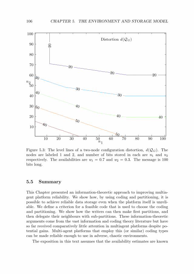
106 CHAPTER 5. THE ENVIRONMENT AND STORAGE MODEL
10
10
2020
20
20
20
20
30
30
30
30
30
4040
40
4040
40
50
50
50
50
50
60
60
60
70
70
80
80
90
90
100
100
n
n1
2
Distortion d(QG)
Figure 5.3: The level lines of a two-node configuration distortion, d(QG). Thenodes are labeled 1 and 2, and number of bits stored in each are n1 and n2
respectively. The availabilities are w1 = 0.7 and w2 = 0.3. The message is 100bits long.
5.5 Summary
This Chapter presented an information-theoretic approach to improving multia-gent platform reliability. We show how, by using coding and partitioning, it ispossible to achieve reliable data storage even when the platform itself is unreli-able. We define a criterion for a feasible code that is used to choose the codingand partitioning. We show how the writers can then make first partitions, andthen delegate their neighbours with sub-partitions. These information-theoreticarguments come from the vast information and coding theory literature but haveso far received comparatively little attention in multiagent platforms despite po-tential gains. Multi-agent platforms that employ this (or similar) coding typescan be made reliable enough to use in adverse, chaotic environments.
The exposition in this text assumes that the availability estimates are known

5.5. SUMMARY 107
for all the nodes. In practice the estimates may be costly to obtain. It may beacceptable that a lower bound on the availability estimates is substituted. Thesecan be obtained at comparatively little cost, by sub-dividing the nodes basedupon the proximity to the writer, and then considering only a subset of possi-ble ways that a node can be accessible to the writer. Apart from yielding theavailability estimates, the sub-division can give rise to a distributed control algo-rithm, whereby once determined, the partition is allowed to dynamically changeto compensate for changes in the network connectivity. This algorithm and itsproperties are recommended for further work.


Chapter 6
Core Based Tree (CBT)
6.1 Introduction
A method for a fully distributed solution to the SDP for a MASs under localizedradio-based communication is described here. Informally, the SDP is the taskof finding, between a set of producers and consumers of services those whichare compatible, i.e. have an overlapping set of product (for the producers) andconsumption (for the consumers) summaries.
The MASs considered here are established by connecting computational re-sources with a commercial, off-the-shelf wireless network. It is assumed for sim-plicity that each such resource (hereafter a node) hosts only a single softwaremodule (an agent), that computes a partial result1 of a computational task. Thepartial result can be communicated to agents at other nodes. The agents mustexchange the partial results in order to complete the entire task. The networkused to connect the nodes is established by radio-based network devices (e.g. con-forming to IEEE 802.11). Due to the interference and the path loss2 of radionetworks, any given node is only able to communicate with the few nodes thatare geographically close to it. The only way to contact the nodes which are notreachable directly is by hopping through a sequence of intermediate nodes, whereeach adjacent pair of nodes are directly reachable. Each path taken between apair of such nodes is called a hop. For a given node in the network, the number ofthe close by nodes (neighbours) is typically far less than the number of all nodesreachable through multiple hops. If the nodes can change their positions overtime, a mobile network is obtained. Such a network is usually called a MANET.
1A partial result is an object constituting a part of a distributed computation. A distributedcomputation is an interleaving of the productions of partial results by nodes and the appropriatedelivery of the partial results between nodes.
2The property of radio signals that their intensity decreases with the distance to the source.As the signal intensity decreases, the Signal-to-Noise Ratio (SNR) worsens, thus making suc-cessful signal detection more difficult with the increase in the distance from the source. Theresult is that radio-based connections exibit strong locality.
109

110 CHAPTER 6. Core Based Tree (CBT)
The MANETs have little initial structure. Typically, the only information anode has from the MANET itself is the set of its neighbours. It is assumed herethat a node in the MANET maintains a current view of the neighbour set by somesensing method. Knowing the neighbours is of course not enough to guaranteethe meaningful communication of partial results between agents. This is because:
1. The agents that need to communicate can be at a distance greater than onenetwork hop so they cannot directly confer. This is due to the MANETproperties and the decaying power of the radio transmission with distance.
2. The agents that need to communicate must determine which partial re-sults should be communicated to which agent, knowing only the summaries,i.e. rough descriptions of the partial results that are being communicatedthrough the network. This is because the network addresses, which en-code the node’s position within a network, have a short life-span due to thechanges in the MANET connectivity.
The latter issue, called the Service Discovery Problem (SDP), is in the focusof this Chapter. Further in the Chapter the special properties of the SDP in theMANET environment are described.
Service Discovery
Service discovery is the name for a collection of techniques by which it is deter-mined at runtime which nodes of a distributed system need to communicate. Theservice discovery precedes any actual data exchange. There usually exist sets ofnodes that produce data objects (producers) and another node that consumesthe same data object (consumers). The goal of service discovery is to convertthe specification of the data object (i.e. a service description) provided by theconsumer into a handle (i.e. identifier) by which the producer of the data can becontacted. Service discovery is one of the resolution mechanisms in routine usedin the Transport Control Protocol (TCP)-based networks. The Domain NameService (DNS) is an example of such a mechanism.
Example 11 (DNS) The DNS, i.e. the naming service used on the Internet isa rudimentary service discovery mechanism. It converts the information need, inform of an URL of an object into an Internet Protocol (IP) address that can beused to contact the object provider.
Every time before a consumer accesses an URL (such as: www.google.com), itmust address a DNS instance with an inquiry for an IP address. In this particularcase (see Figure 6.1), a set of equivalent IPs is returned, with auxiliary data someconsumers may find useful. After having obtained the IP number, the consumercan use it to address the producer directly by its network address.
Thus, before actual communication occurs, an additional round of inquiriesmust take place, in which a consumer determines which producer can tend to its

6.1. INTRODUCTION 111
; <<>> DiG 9.3.1 <<>> www.google.com
;; global options: printcmd
;; Got answer:
;; ->>HEADER<<- opcode: QUERY, status: NOERROR, id: 30373
;; flags: qr rd ra; QUERY: 1, ANSWER: 4, AUTHORITY: 6, ADDITIONAL: 6
;; QUESTION SECTION:
;www.google.com. IN A
;; ANSWER SECTION:
www.google.com. 620 IN CNAME www.l.google.com.
www.l.google.com. 156 IN A 66.102.9.99
www.l.google.com. 156 IN A 66.102.9.104
www.l.google.com. 156 IN A 66.102.9.147
;; AUTHORITY SECTION:
l.google.com. 63598 IN NS g.l.google.com.
l.google.com. 63598 IN NS a.l.google.com.
l.google.com. 63598 IN NS b.l.google.com.
l.google.com. 63598 IN NS c.l.google.com.
l.google.com. 63598 IN NS d.l.google.com.
l.google.com. 63598 IN NS e.l.google.com.
;; ADDITIONAL SECTION:
a.l.google.com. 63875 IN A 216.239.53.9
b.l.google.com. 63875 IN A 64.233.179.9
c.l.google.com. 63875 IN A 64.233.161.9
d.l.google.com. 63875 IN A 64.233.183.9
e.l.google.com. 63875 IN A 66.102.11.9
g.l.google.com. 63875 IN A 64.233.167.9
;; Query time: 5 msec
;; SERVER: 130.161.180.1#53(130.161.180.1)
;; WHEN: Thu Feb 2 15:58:32 2006
;; MSG SIZE rcvd: 292
Figure 6.1: The standard response of a DNS server, when queried for a servernamed www.google.com.

112 CHAPTER 6. Core Based Tree (CBT)
information need. The service that generalizes service discovery is named YellowPage Service (YPS). The YPS translates service descriptions (infomation needs)into Unique Identifiers (UIDs) of the receivers that offer the service matching thisneed.
We describe in brief two typical methods for building the YPSs, the CentralizedYPS and Broadcast YPS. We then describe in brief an improved schema that wecall the Minimally Distributed YPS, which relies on the environment model asbuilt in this text.
Centralized YPS
A fixed subset of nodes is chosen to keep and update the service descriptions. Thecentralized YPS is the solution with the simplest structure of all. As the YPSdelivers UIDs, representing the network-layer address of the receiver, stale UIDoften means that by the time YPS is finished resolving, it is impossible to refer tothe receiver as its position in the network is changed. This problem is pronouncedin MANETs, where nodes can move about freely. Even when YPS is possible, itis still required for each client to have a network address of the YPS to be ableto ask it for service.
Thus, introducing an indirection via YPS solves the information need basedmatching, but does not solve the tight coupling for the YPSs themselves. More-over, the YPS node becomes a single point of failure. The outage of the YPSserver means that its data must be rebuilt again elsewhere.
Broadcast YPS
Each node advertises its services to a subset of nodes that are closest with respectto some distance measure (such as network distance). A network-wide policy onfurther dissemination of service advertisements is adopted, by which is determinedhow the service descriptions are propagated.
The simplest distribution policy is that where all the service descriptions arepropagated to all the nodes in the network. While this policy removes the singlepoint of failure, it introduces the problem of the communication overhead andhousekeeping of all the service descriptions across the entire network.
Minimally Distributed YPS
The minimally distributed YPS uses the smallest possible number of links for theservice advertisements. This requires that a spanning tree structure is constructedand maintained throughout the network lifetime. For this purpose, the construc-tion and maintenance of a spanning-tree strucure named CBT is presented.

6.1. INTRODUCTION 113
Use Cases
The MANET scenario arises often, in practice and in the scientific studies alike.Diverse examples are given, that either use MANET or a network with similarproperties for the communication. In these examples no fixed communicationinfrastructure is assumed to exist.
Sensor Networks. The sensor networks are formed by small measurementdevices. These devices are equipped with sensors that measure various physicalquantities (e.g. temperature, pressure, humidity), and a radio transceiver that cancommunicate and receive the measurements. The devices are “liberally sprinkled”in a target area. The MANET is used for communication between the nodes. TheSDP in sensor network is trivial, and consists of forwarding the data from all thesensors to a single collection point.
Systems-on-Chip (SoC). The SoC are complex integrated circuits that com-bine a possibly large number of diverse circuits on a single silicon die. In sucha system, it has been determined that simple bus-type connections yield perfor-mance bottlenecks and the networking approach is suggested. There is consid-erable interest in the research community for building a local interconnect forSoCs. The interconnect has MANET locality properties, although the physicaldata transfer uses metal layers rather than radio. The SDP for SoC consists offinding data paths.
Rescue Operations. The use of information technology in rescue operationshas received increased interest in recent years. The participants in the near fu-ture rescue operations may be equipped with portable computers (e.g. PDAs)that will be used for critical data exchange, and to coordinate action. Such de-vices will expand the role of radio stations (e.g. walkie-talkie) from exchangingvoice messages to full integration with the supporting information systems. It isreasonable to expect that such PDAs will be able to exchange data through radiolinks between themselves. These devices need not rely on the existing communi-cation infrastructure. Rather, the devices need to be able to set up a MANETand cooperate in message delivery. The SDP for rescue operations consists offinding clusters of PDAs that need to communicate.
Contribution
The core contribution of this Chapter is in the new use of the structure knownas the Core Based Tree (CBT) for providing the dynamic service discovery struc-ture. Further, the detailed account of the CBT construction and maintenancealgorithms, in the relaxed requirements context (i.e. allowing the appearance ofunicycles) is novel to the best of our knowledge. Finally, using the Z and CPNframeworks to describe particular aspects of the algorithms (Z for describing thestate changes, and CPN for handling concurrency) is novel to a limited extent.Since the state evolution of systems and concurrentcy handling is a recurringtopic in the analysis of algorithms, there exist equivalent formalisms, which have

114 CHAPTER 6. Core Based Tree (CBT)
been used in various contexts: for instance, CSP in [40], CPN in [69], and CSPand Object-Z in [76].
The choice for CPN and Z stems from the straightforward way the presentedalgorithms are implemented in the used development platform, the COUGAARframework [10].
Related Work
Papers describing related work can be roughly divided into three classes:
1. Papers that discuss service discovery in MANETs;
2. Papers about event notification (i.e. delivery of “event” objects to interestedparties in a distributed setup); and
3. Papers about CBT in the context of Internet multicasting.
As reported in [65], the service discovery in MANET is organized as beingeither service coordinator based where designated nodes collect the service sum-maries (e.g. Jini [55], or virtual backbone approach of Kozat and Tassiulas [45]);or distributed query based, where service discovery requests are flooded throughthe MANET with respect to some flooding scope parameter (e.g. the electrostaticfield based approach of [49], or efficient flooding of [67]); or hybrid (e.g. [73]),combining the former two approaches.
Our approach to SDP differs sharply from those given above as it avoids servicecoordinators as well as query flooding, reasons following.
First, the existence of service coordinators does not really solve the SDP forMANET, since the real issue is finding an efficient way to distribute the servicedescriptions, rather than the coordinator election. Even when coordinators arepresent, the problem of connecting them remains and is of the same type as theoriginal SDP, although fewer nodes participate.
Second, query flooding as a way to compensate for not knowing the targetposition has scalability problems. However, it is the only way out as in MANETit is not known where the service queries need to go. Instead of flooding, a minimalstructure is maintained that guarantees the participation of all the MANET nodes,and define a policy for forwarding the service descriptions over it. To achieve this,it is required that nodes in the CBT provide the descriptions of both the offered,and the required services.
The event notification has been extensively studied in the context of publish-subscribe middleware. Examples thereof are Gryphon [38] and Siena [17]. Con-trary to our approach, these event notification systems are intended for use in afixed network and hence do not need to construct a structure for service descrip-tion propagation. However, they contain useful ideas which served as startingpoints in our work. These are the notions of service summaries and approximateservice matching, introduced in [17], and analyzed independently in [91]. Applica-tions of the efficient summaries under reconfiguration of the distribution structure
6.2. PROBLEM DESCRIPTION 115
(analogous to topology changes in a MANET that is studied) was treated in [66]which are also considered feasible for MANETs.
The CBT structure is described in [9]. In that paper it is used as a wayof space-efficient internet multicasting. Instead of building a multicast tree foreach multicast session, the seminal CBT paper proposes using a single tree for allthe sessions, thus simplifying the build up of the multicast infrastructure, at theexpense of some extra incurred traffic.
The CBT idea is used in the modified context (i.e. MANETs) to make adistributed structure akin to a spanning tree, that is then used to guaranteesuccessful service discovery. Making and maintaining the CBT turns out to besimple enough to be performed efficiently in a MANET. It represents a distributedspanning tree construction with the requirements somewhat relaxed compared tothe original spanning tree problem formulation (Gallager et al. [34]).
6.2 Problem Description
Preliminaries
The basic type considered is called Node. It represents any system node. It isintroduced as an opaque type as its internal structure does not play a role in thespecification.
[ Node ]
The resource and network setup are described in terms of a family of graphsΓ, each member consisting of nodes and the connections:
Γ : R→ P Node × (Node ↔ Node)
Each member of the family Γ is a graph represented by a pair (V : PNode,E :Node ↔ Node). Each element of V stands for a node and (with a tolerable abuseof notation) the co-located agent. E is a symmetric binary relation on V , andrepresents the nodes that can directly communicate between each other (hencethe connections are always bi-directional). The family members of Γ are indexedby time. For a real t , Γ(t) is the graph corresponding to the available nodes andconnections at time t . Hence, Γ describes the temporal evolution of the network.Note that only a part of Γ can be retrieved at a given time t . This part consistsof all Γ(t ′) such that t ′ ≤ t . It is assumed that each node can detect other nodesthat it can directly communicate to. Call this the neighbours set.
N : Node → (R→ P Node)
Given a node v : Node, and some time point t : R, then Nv (t) is the set ofneighbours of v at time t . An obvious connection exists between N and Γ, suchthat n : Node is only allowed to be a neighbour of v at time t if for Γ(t) = (V ,E )it holds that (n, v) ∈ E .

116 CHAPTER 6. Core Based Tree (CBT)
Each agent specifies the type of partial results that it accepts from otheragents. Likewise it specifies the type of partial results that it produces for theother agents. The partial results considered here are drawn from a set of allconstructible types, the dataspace:
[ Dataspace ]
Hence all partial results are of the form x ∈ Dataspace. A node gives adescription of all the partial results through predicates. Two predicate classes areused per agent. One detailing the acceptable elements of the dataspace, the otherdetailing the producible elements of the dataspace.
φc , φp : Node 7→ P Dataspace
Call the former the consumer summary, and call the latter the producer sum-mary. For an agent v they are denoted as φc
v and φpv respectively. For simplicity
it is assumed that they do not change. The element sets of the intersection andunion of two summaries φ1 and φ2, denoted as φ1 · φ2, and φ1 + φ2 respectivelydefine the sets:
φ1 · φ2 = φ1 ∩ φ2
φ1 + φ2 = φ1 ∪ φ2
A producer summary φpv of a node v and a consumer summary φc
w of a nodew are compatible if φv · φw is a nonempty set.
Problem Formulation
Now the SDP can be defined:
Definition 9 (Service Discovery Problem) Let t ∈ R be a point in time. Letthere be given a set of nodes and a family Γ as described. Let the families φp andφc be given. For each pair of nodes v and w such that φp
v and φcw are compatible,
find a path in Γ(t) connecting v and w. Also notify v that w has been found, andvice-versa.
By Definition 9, the SDP is a task continuously solved during the MANETruntime. The solution of the SDP allows any agent v to query whether thereexists an agent w with a compatible service description. Once it is found, v canaddress w to render the advertised service. In a MAS an agent typically needsthe rendition of the service rather than the contact with a particular agent byname, hence the need for this lookup by service.
Relevance
Lookup by service is typically [85, 10] realized in MAS as some form of a database,centralized for simplicity. This is a drawback in the MANET settings as reported

6.3. SOLUTION OUTLINE 117
in [49]: “Service discovery in [MANET] is challenging because of the absenceof any central intelligence in the network. Traditional solutions as used in theInternet are hence not well suited for [MANET].”
The SDP is an important component in the functioning of any MAS platform.It is a link between the distributed application running on a MAS, where agentsconnect based on the compatibility of their service summaries, and the networklayer which is typically able to communicate messages between nodes identifiedby name. In a MAS that relies on a fixed node and network infrastructure, SDPcan be solved to an acceptable level by database lookups [10]. In MANETs wherethe fixed node and network infrastructure assumption must be removed, the wayto solve SDP becomes less obvious, although still crucial for the MAS operation.This importance of having an efficient solution to SDP for the MAS deployedon MANETs, without central coordination, is the main motivation for the workdescribed in this Chapter, and it is viewed as an enabler for a wide range ofMANET-based distributed applications.
The SDP as given in the Definition 9 is a compact formulation of a problemthat arises frequently in MASs. A typical MAS consists of agents that bothexport services to the community and require services from other agents to work.In this context, a service consists of delivering some objects from Dataspace fromthe producer agent to the consumer agent. A consumer agent x that requires aservice s can contract any produced agent y which can provide s . The consumerx does not care about which y is allocated to service s , as long as the service isrendered. It is said that x performs a lookup by service. The need for the lookupby service implies that a mapping must exist between service descriptions and theagents that offer this service. By analogy with telephone directories, such mappingis called the YPS (and is itself offered as a service). One approach of making theYPS is providing a registry that contains all the services and has an up to datemapping to the agents that implement them. The simplest form of the YPSregistry uses a centralized database to store the service descriptions. For a largeMAS a centralized database is a performance bottleneck and implementationsconsider distributed YPS that ameliorate the issue. Depending on the way thedistribution is performed, the YPS servers may require some network traffic tosynchronize their local registries. It is also required that the registry locations areknown in advance. The database approach has a weakness when the underlyingnetwork is a dynamic MANET. In a dynamic environment it is not obvious wherethe YPS is to be hosted. The YPS locations are also out of reach for externalconfiguration.
6.3 Solution Outline
The solution is proposed of the SDP by using a fully distributed data structurebased on the Core Based Tree (CBT), and a detailed account is given how thestructure is made and maintained. Before the solution analysis, its informal out-

118 CHAPTER 6. Core Based Tree (CBT)
line is given to explain what is achieved in the detailed algorithm description.The approach is in view of several requirements and assumptions as follows. Re-quirements for the data structure:
1. Scalability. Must operate efficiently with respect to the number of nodes;
2. Simplicity. Must be able to include new nodes in the structure by consid-ering locally available information only; and
3. Repairability: Must be easily repairable in face of changes in network con-nectivity.
Assumptions:
1. Slowly changing environment. The CBT maintenance never terminates inthe classical sense, constantly adapting as the connectivity changes, with theCBT property only partially fulfilled during adaptation. Frequent changesincrease the probability that the CBT algorithm needs to adapt the CBT.Hence dynamics must be limited for the CBT properties to be fulfilled; and
2. Infrequent change in service summaries. Hence the change due to servicedescription forwarding is localized only to parts of the CBT. This facilitatesthe CBT repair.
The CBT is used to provide a minimal communication structure offering fullconnectivity. The CBT is built implicitly: the nodes that form the CBT keep onlya small amount of soft state that is used for local decision making. The CBT doesnot need to be stored entirely at any one node. The minimality stems from thescalability requirement, as the resulting structure must be easy to bookkeep, andrequire low bandwidth to manage. A tree-like structure follows naturally fromthese requirements.
The CBT is considered only as a structure for solving the SDP. The method isunsuitable for communicating the content as the traffic volume over the structureis not balanced. Thus using the CBT is proposed to solve the SDP, thereafterusing any routing method appropriate for ad-hoc networks for content communi-cation.
Core Based Tree (CBT)
For the rest of the exposition, Γ is assumed to be a family of connected graphs.Otherwise, assuming that for some t the Γ(t) is disconnected, the given solutioncan be simply applied to all the connected components in turn. The solution isthen valid within these components only.
The CBT is a weakly-connected3 directed spanning tree over the set of nodes Vthat induce the graph Γ(t) = (V ,E ) for some t (see the Figure 6.2 for illustration;
3A graph is weakly-connected if it is directed and there exists a pair of nodes u and v forwhich an oriented path exists either from u to v or v to u but not both.
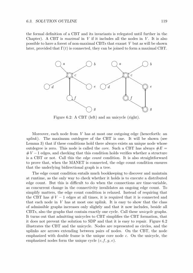
6.3. SOLUTION OUTLINE 119
the formal definition of a CBT and its invariants is relegated until further in theChapter). A CBT is maximal in V if it includes all the nodes in V . It is alsopossible to have a forest of non-maximal CBTs that exaust V but as will be shownlater, provided that Γ(t) is connected, they can be joined to form a maximal CBT.
76540123 a
??
????
76540123 b
xxrrrrrrrrr
76540123'&%$ !"# c
76540123 d
77oooooooooo 76540123 e
ffLLLLLLLLL
76540123 f
OO
76540123 g
ffLLLLLLLLL
76540123 a
??
????
76540123 b
xxrrrrrrrrr
76540123'&%$ !"# c
76540123 d
77oooooooooo 76540123'&%$ !"# e
ffLLLLLLLLL
76540123'&%$ !"# f
&&LLLLLLLLL
76540123'&%$ !"# g
OO
Figure 6.2: A CBT (left) and an unicycle (right).
Moreover, each node from V has at most one outgoing edge (henceforth: anuplink). The maximum outdegree of the CBT is one. It will be shown (seeLemma 3) that if these conditions hold there always exists an unique node whoseoutdegree is zero. This node is called the core. Such a CBT has always #E =#V −1 edges, and checking that this condition holds verifies whether a structureis a CBT or not. Call this the edge count condition. It is also straightforwardto prove that, when the MANET is connected, the edge count condition ensuresthat the underlying bidirectional graph is a tree.
The edge count condition entails much bookkeeping to discover and maintainat runtime, as the only way to check whether it holds is to execute a distributededge count. But this is difficult to do when the connections are time-variable,as concurrent change in the connectivity invalidates an ongoing edge count. Tosimplify matters, the edge count condition is relaxed. Instead of requiring thatthe CBT has #V − 1 edges at all times, it is required that it is connected andthat each node in V has at most one uplink. It is easy to show that the classof admissible graphs increases only slightly and that it now includes, beside allCBTs, also the graphs that contain exactly one cycle. Call these unicycle graphs.It turns out that admitting unicycles to CBT simplifies the CBT formation, thatit does not prevent the solution to SDP and that it is easy to repair. Figure 6.2illustrates the CBT and the unicycle. Nodes are represented as circles, and theuplinks are arrows extending between pairs of nodes. On the CBT, the nodeemphasized with double frame is the unique core node c. On the unicycle, theemphasized nodes form the unique cycle (c, f , g, e).

120 CHAPTER 6. Core Based Tree (CBT)
CBT Construction and Maintenance
There are two main classes of events at runtime, where the CBT structure needsto be adjusted.
1. On initialization. Initially, the nodes of V are partitioned into V non-maximal CBTs, with only a single node each. A sequence of join operationsis performed on the non-maximal CBTs until a maximal CBT is obtained.
2. On change. Whenever the connectivity of Γ(t) changes and as a consequencethe CBT conditions are violated, the resulting structure must be repaired.This happens when the connectivity structure in Γ(t ′) changes with respectto Γ(t) for some t ′ > t .
The CBT instantiation boils down to adopting an uplink for all the nodes inV , such that the CBT obtained at the end is maximal. This process exibits goodstructure, in the sense that the maximal CBT can be obtained by repeatedlyjoining smaller CBT. Hence our approach is to find and join in a distributedmanner pairs of non-maximal CBTs. The join operation thus needs to performthe following:
1. Find two CBTs (say G and H ) such that there exist edges in Γ(t) that startat a vertex of G and end at a vertex of H (or vice-versa).
2. Denote the set of such edges as EGH . From EGH adopt exactly one edge(say eGH ) to connect G and H .
3. Adjust the edges in the union of G and H with eGH added, and the positionof the core nodes such that the obtained graph is a CBT again.
The join is divided into four distinct phases. Each phase represents a transac-tion that partially adjusts the CBT. As usual, the operations within a transactionare applied atomically to the CBT when a transaction is committed. Conversely,the operations within a transaction are not applied at all if the transaction isaborted. Within the bounds of a single transaction, the participating nodes areallowed to temporarily break the CBT invariants where appropriate. However,upon transaction commit, the resulting structure must fulfill the CBT invariants.The join unfolds in several phases. In Figure 6.3, the phases are named Meet,Vote, Switch and Yield and are described below. The dotted line on each il-lustration represents the CBT boundary. At Meet (top), two nodes belonging todifferent CBTs come into contact and exchange identity information. At Vote thesame two nodes conduct a vote to determine which of the two CBT cores mustyield its function. If the core of the yielding CBT is away from the node, a seriesof Switches are applied until the core node appears at the join. At Yield, the corenode yields its function by adopting an uplink that leads to another component.
1. Meet. This phase is initiated between every pair of nodes that come tocontact. It is used to set the communication up, and determine which node

6.3. SOLUTION OUTLINE 121
is the leader for the join. The meet phase is used to prevent crosstalk(cf. [69], page 45), i.e. a situation in which both nodes either accept, orrefuse to be the leader ad infinitum.
2. Vote. In this phase, the nodes take a vote to determine which of the coresof the two CBT has to yield. It is also used to determine whether a join isfeasible. If yes, the control is passed on to the next phase. If no (such aswhen the nodes belong to the same CBT), the join is cancelled.
3. Switch. The node that executes a yield must be the core node. In case that,after a vote, the yielding node is not also the core, a sequence of Switchoperations is initiated. The goal of each switch is to move the core nodefrom its position to a node. A sequence of such switches is used to movethe core of the yielding component to the join site.
4. Yield. Now that the core node is at the join site, it is enough that it adoptsan uplink towards the far end of the join site. This implicitly removes therole of the core from that node. It can be shown that the resulting graphis a CBT, as required.
Cycle Removal
Several concurrent join transactions may unfold at any given time. As a conse-quence, parallel joins can occur. In Figure 6.4, the cores of the two componentshave each decided to yield (left). The yield directions are given by the dottedarrows. As a result, the obtained structure after the join (right) is an unicycleinstead of a CBT. While parallel joins do affect the CBT structure (in fact, theydestroy it), the resulting graph still provides full connectivity (hence supportingthe solution to SDP), and is easily repaired, by removing a single extra link. Forefficiency reasons the link removal is relegated to the point where the presenceof a core node in a component is essential, i.e. to immediately before the Switchphase. This means that a graph remains an unicycle until it is required to joinwith another.
For the cycle detection to work, it is enough that the cycle is detected atany single node which forms a part of the unique cycle. How this is done willbecome obvious in the detailed discussion of the cycle removal. Once a node(say v) obtains a proof that a cycle exists it can take action to remove the cycle.For instance it may remove the cycle by dropping its current uplink. The nodethus becomes the new core and may resume the usual operations. However, thisapproach has problems when concurrency comes into play. Multiple nodes maydiscover that they are a part of the cycle. If all of them are allowed to assumethe role of the core, the graph would become unnecessarily fragmented, as morelinks would be removed than the minimum of one. This is not the best possibilityalthough it is not catastrophic, as each of the fragments would itself form a CBT.

122 CHAPTER 6. Core Based Tree (CBT)
//76540123'&%$ !"# 76540123oo o/ o/ o/ Meet 76540123 ///o/o/o 76540123'&%$ !"# ooOO OO OO OO
//76540123'&%$ !"# 76540123oo o/ o/ o/ ks Vote +376540123 ///o/o/o 76540123'&%$ !"# ooOO OO OO OO
//76540123'&%$ !"# 76540123oo o/ o/ o/ ksSwitch +376540123'&%$ !"# 76540123oo o/ o/ o/ ooOO OO OO OO
//76540123'&%$ !"# 76540123oo o/ o/ o/ 76540123
Yieldoo 76540123oo o/ o/ o/ oo
OO OO OO OO
Figure 6.3: The phases of the Join operation.
76540123'&%$ !"#
76540123oo
76540123 //76540123'&%$ !"#
OO76540123
76540123oo
76540123 //76540123
OO
Figure 6.4: A parallel join.
An improved approach is to run a leader election algorithm in a ring. Leaderelection in a ring has a known solution ([51], page 475 gives several solutions). Itis known from v that the ring (i.e. the cycle) is implicitly available by following asequence of uplinks from the node that detected it. The node v can then initiatea leader election algorithm which is known to terminate eventually either with asuccess (whereby the elected leader removes its uplink and becomes the core), orwith a failure (whereby the leader election is prevented by the cycle destruction;

6.4. ALGORITHM DESCRIPTION 123
but the cycle destruction is precisely what is wanted in the first place, so thisoutcome also wins).
SDP Strategy Computation
In this section it is assumed that at any given t , the CBT has been constructedon top of Γ(t). Hence, for each node, the uplink is known if it exists.
upl : Node × R 7→ Node
coreof : Node × R 7→ Node
∀ t : R ∃1 v : Node • (v , t) 6∈ dom(upl)
∀ t : R • u = coreof (n, t)⇒ ∃n : N • u ∈ upl( , t)n ∧ u 6∈ dom upl( , t)
Conversely, for a given node the set of downlinks is also defined. That is theset of the nodes that have it as an uplink.
dnl : Node × R 7→ PNode
∀ t : R, v : Node,W : P Node •(v , t) 7→W ∈ upl ⇒ ∀w ∈W • dnl(w , t) = v
For simplicity the changes in the CBT due to changes in Γ(t) are not con-sidered. Thus the time indices in upl and dnl are dropped for some fixed timepoint t . Assume that the nodes have the families φp and φc well defined. As ashorthand φx will be used, where x ∈ p, c ranges over both summary types. Asthe CBT is hierarchical it is possible to aggregate the summaries as follows. Thesummary distribution unfolds in two interleaved phases. The first phase is theconvergence, consisting of messages which get sent towards the CBT core. Thesecond phase is the divergence, consisting of messages flowing from the core tothe leaf nodes.
In the convergence phase, the leaf nodes forward the two summaries to thecorresponding uplink. The non-leaf nodes collect summaries from their downlinksand make an aggregate with their own respective summaries by first computingan union and thereafter simplifying the resulting summaries where appropriate.The result of these operations are forwarded on to the CBT core.
In the divergence phase, a node examines the received summaries for compat-ibility. Compatible summaries have a non-empty intersection. Consider a node vfor which two different nodes are downlinks as follows: w , u ∈ dnl(v),w 6= u. Ifφpwφc
u 6= ∅, then v produces φpwφc
u and forward each to w and u. Similar matchingoccurs for v and w to handle the case when v and w are compatible.
6.4 Algorithm Description
In this section, the CBT formation and the summary matching algorithms aredescribed in detail.
124 CHAPTER 6. Core Based Tree (CBT)
Preliminaries
Here it is assumed that the graph G = (V ,E ) is a member of the family Γ, i.e.there exists some t : R such that G = Γ(t). The label T is used when it is impor-tant that the graph has a special property (i.e. be a tree, or CBT, or unicycle).The standard terms for graphs are used throughout (see for instance [25]). Firstit is specified what is meant by CBT and Unicycle. Thereafter a connection isgiven between the two, also permitting the maintenance of a relatively weak set ofinvariants for the CBT construction, provided that it is known how to remedy anyunwanted side effects when the CBT degenerates into an unicycle. The followingProposition specifies the invariants of a CBT.
Proposition 5 (Core Based Tree Invariant) Let there be given a digraph4
T = (U ,H ), with U the set of nodes, and H the set of edges on U . T is aCore Based Tree (CBT) if the following hold in T:
1. The underlying5 graph is a tree.
2. Any node u ∈ U has at most one uplink in T.
Definition 10 (Unicycle) A unicycle is a weakly-connected digraph that hasexactly one cycle.
Lemma 2 (Directed Acyclic Graph (DAG) Endpoints) Any DAG has atleast one source node and at least one sink node.
Proof. Without loss of generality, consider only the sink nodes. Let the numberof nodes in the DAG be n and suppose the contrary, that no node is a sink. Thenfor each node, there is at least one outgoing edge. Follow an outgoing edge to anew node. Repeat the procedure n + 1-times to obtain a path of length n + 1.As there are n nodes, by Dirichlet principle there is a node that has been visitedtwice. Thus a loop exists, and the graph is not a DAG, a contradiction. Use thesame argument to prove at least one source node exists.
Lemma 3 A connected CBT has an unique core node.
Proof. Let the CBT consist of n nodes. The core node of an CBT must be asink. By Lemma 2, an CBT has at least one sink. As the CBT is connected, thereexist n − 1 uplinks. Map each uplink to the node it emanates from. Neither ofthese n−1 nodes is a sink as it has an emanating uplink. Then the only remainingnode must be a sink and is therefore the unique core.
Proposition 6 (Similarity between CBT and Unicycle) Let T = (U ,H )be a weakly-connected digraph. Let for each u ∈ U be #upl(u) ≤ 1. Then U iseither a CBT or a unicycle.
4A directed graph. In a digraph the edges have a beginning and an ending node.5For a directed graph, the underlying graph is its undirected version, i.e. the same graph
with the edge directions dropped.

6.4. ALGORITHM DESCRIPTION 125
From the Proposition 6 it is seen that the properties of T that the CBTalgorithm must take care of are:
1. Ensure T is weakly-connected;
2. Ensure that for each u ∈ U , #upl(u) ≤ 1; and
3. Ensure that there exists at least one u ∈ U that can locally decide whetherT is a CBT or a unicycle.
The Meet Protocol
The meet protocol is first executed when node neighbourhood changes. Before anymessage exchange can occur between a pair of new neighbours, the conversationinitiator must be established. This prevents the occurrence of a synchronizationproblem known as crosstalk, whereby both nodes either take the initiative orboth nodes wait for the other to start. In Figure 6.5, the PN that realizes theMeet with crosstalk detection is shown6. The place and transition abbreviationsare as follows: U : Undetermined (The state of the agent is undetermined: itis not yet known whether the node must assume the role of the Client or theServer); sr : Send Request; PA: Pending Answer; RR: Received Request; arc:Accept Role Client; rc: Role Conflict; CR: Conflicted roles mean that there is a(temporary) conflict between roles of A and B); vc: vote for client – this agenthas decided to become a client; vs : vote for server – this agent has decided tobecome a server; PAC : Peer Accepted Client – this agent has been notified thatits peer has accepted to become a client. Thus becoming the server is safe. apc:Acknowledge Peer as Client – acknowledge that the peer agent assumed the roleof a Client in the interaction; RC : Role Client – the agent has accepted the roleof a client; RS : Role Server – the agent has accepted the role of a server.
As the Figure 6.5 shows the interaction of two agents, the places and transi-tions in this diagram and onwards are annotated with a lower index A or B , toemphasize the agent to which they belong. The indices will be dropped in thelater CPN figures if the distinction is not relevant or is handled in another way7.Further, throughout the diagrams, the same labels are used for one and the sameplace. Hence, the given CPN fragments can be attached together to form thecomplete CPN by overlapping all the places bearing identical names.
Theorem 6 (Crosstalk Detection) Let Agents A and B execute the Meet pro-tocol as given in the network Σ6.5 in Figure 6.5. The following holds:
Σ6.5 ⊢ UA UB → (RCA ¬ RSA ¬ RCB RSB) ∨ (¬ RCA RSA RCB ¬ RSB). (6.1)
6Refer to Chapter 2 for the details of the CPN notation.7This distinction can also be handled by means of folding.

126 CHAPTER 6. Core Based Tree (CBT)
76540123• UA
76540123• UB
**
****
****
****
****
****
****
****
srA
++WWWWWWWWWWWWWWWWWWWWWWWWWWWWWWWWWWWWWWWW srB
ssgggggggggggggggggggggggggggggggggggggggg
76540123PAA
44
4444
4444
4444
4444
4444
4444
4444
4444
76540123RRA
•
__????????????
wwoooooooooooooooooooo
76540123RRB
•
??
??
????
????
??
''OOOOOOOOOOOOOOOOOOOO 76540123PAB
arcA
**
****
****
****
****
****
****
****
++WWWWWWWWWWWWWWWWWWWWWWWWWWWWWWWWWWWWWWWW rcA
rcB
arcB
ssgggggggggggggggggggggggggggggggggggggggg
76540123CRA
??
????
????
??
76540123PACA
76540123PACB
76540123CRB
vcA
vsA
apcA
apcB
??
????
????
??vsB
vcB
76540123RCA76540123RSA
76540123RSB76540123RCB
Figure 6.5: The Petri Net diagram of the Meet protocol between two agents, Aand B .
Proof. The protocol unfolds until a decision about the role assignment has beenreached. We first inspect the proof graph of finite length, given in Figure 6.6.The proof graph shows the causes relations that hold between the states of theCPN from the Figure 6.6. As the given CPN is symmetrical with respect to thepermutation of agents A and B , we need to consider only one of the possible twofirst transitions. That is, in the Figure, only the firing of the transition srB isconsidered, as the case in which srA occurs gives the same proof graph, but withthe agent names A and B interchanged.
Knowing this, the following reasoning leads to the proof of Equation (6.1).The derivation steps use the basic CPN triggering rules, which follow immediatelyfrom Σ6.5. The symmetry of Σ6.5 is used throughout.

6.4. ALGORITHM DESCRIPTION 127
UA UB // UA RRA PAB w
))TTTTTTTTTTTTT // RRB PAB RRA PAA
// CRA CRB _
t
''OOOOOOOOOO
RCA PACB PAB v
))SSSSSSSSSSSS RCA CRB _
CRA RCB _
RCA RSB RSA RCB
Figure 6.6: The crosstalk detection proof graph in the Meet protocol, for thenetwork Σ6.5.
First note that due to the CPN activation rules and the sequence of transitionsleading from UA to RCA and RSA, the following holds:
Σ6.5 ⊢ UA + PAA + CRA + RCA + RSA = 1⇒ RCA + RSA ≤ 1. (6.2)
The right-hand side of the rule states the mutual exclusion of the client and serverstates of A. By symmetry, the analogous claim holds for the B -part of Σ6.5:
Σ6.5 ⊢ RCB + RSB ≤ 1. (6.3)
Consider now the state in which Σ6.5 ⊢ RCA holds. There are two ways this mighthave happened, either via arcA, or via vcA. Therefore the following holds:
Σ6.5 ⊢ RCA ⇒ (PACB + RSB = 1) ∨ (UB + PAB + CRB + RSB = 1).
The second part of the right hand side due to the assumed consensus betweenvcA and vsB , which is externally ensured through voting. Assuming progress onall transitions, eventually either PACB = 0, or UB + PAB + CRB = 0, yielding inboth cases:
Σ6.5 ⊢ RCA ⇒ RSB = 1⇔ 0 ≤ RCA ≤ RSB ≤ 1. (6.4)
Substituting from here RCA instead of RSB into Equation (6.3), we obtain:
Σ6.5 ⊢ RCA + RCB ≤ 1, (6.5)
proving mutual exclusion of the decisions in which both agents decide to be clients.Further, from adding Equation (6.2) and Equation (6.3), and taking into accountEquation (6.5), one obtains
Σ6.5 ⊢ RCA + RCB + RSA + RSB ≤ 1 + RSA + RSB ≤ 2, (6.6)
from where we get:
Σ6.5 ⊢ RSA + RSB ≤ 1, (6.7)

128 CHAPTER 6. Core Based Tree (CBT)
representing the mutex condition for the server decision for both agents. Finallywe have:
Σ6.5 ⊢ RSA+RSB ≤ 1 ∧ RCA + RCB ≤ 1
⇒(RCA ¬ RSA ¬ RCB RSB) ∨ (¬ RCA RSA RCB ¬ RSB),(6.8)
thus proving the claim of Theorem 6.
The Vote Protocol
The Vote protocol determines for a pair of nodes which one will be required toyield. The node that loses the vote is required to notify the core of its correspond-ing component that it must be disbanded i.e. that it must yield its functions toanother (Figure 6.7). The vote requires both nodes in the pair to agree on a value
76540123• RS
76540123• RC
//
76540123C
//
76540123 A
76540123 B
76540123 D
??
????
??
q q
q
q
76540123YRA76540123YRB
Figure 6.7: The Vote protocol.
of some predicate, shown as q in the Σ6.7. As the outcome of a vote, only one ofthe nodes may start the yield request. Hence, only one of the two yield requests(shown in Figure 6.7 as YRA and YRB) may be activated.
Theorem 7 (Vote) Let there be given a PN as in Σ6.7. Then the followingholds:
Σ6.7 ⊢ YRA + YRB ≤ 1.
Proof. From Σ6.7, the following hold:
Σ6.7 ⊢ q ⇒ YRB = 0 ∧ RS + A + YRA = 1
Σ6.7 ⊢ q ⇒ YRA = 0 ∧ RC + D + YRB = 1,

6.4. ALGORITHM DESCRIPTION 129
since q = true implies that the transition leading to YRB never executes, and thatthe transition sequence leading to YRA must occur eventually (and vice-versa, forq = false). Hence, first:
Σ6.7 ⊢ q ⇒ YRB = 0 ∧ RS + A + YRA = 1[ RS ≤ 1 ∧ A ≤ 1 ]
Σ6.7 ⊢ q ⇒ YRB = 0 ∧ YRA ≤ 1
Σ6.7 ⊢ q ⇒ YRA + YRB ≤ 1.
Thereafter, similarly:
Σ6.7 ⊢ q ⇒ YRA = 0 ∧ RS + C + D + YRB = 1
[RC ≤ 1 ∧ C ≤ 1 ∧ D ≤ 1]Σ6.7 ⊢ q ⇒ YRB = 0 ∧ YRA ≤ 1
Σ6.7 ⊢ q ⇒ YRA + YRB ≤ 1.
Finally, collecting the two conclusions:
Σ6.7 ⊢ q ⇒ YRA + YRB ≤ 1
Σ6.7 ⊢ q ⇒ YRA + YRB ≤ 1
[(ϕ⇒ µ ∧ ϕ⇒ µ)⇒ µ]Σ6.7 ⊢ YRA + YRB ≤ 1.
Also note that Σ6.7 ⊢ YRA+YRB = 1 → RC = 0 ∧ RS = 0 assumes progress,i.e. it is assumed the said transition eventually occurs.
The Switch Protocol
In this section, claims are made about the environment in which the nodes (andthe co-located agents) operate, as well as the internal soft states of the nodes. Toachieve this, all the nodes must be considered at once. This is achieved by folding(see [69]) all the local CPNs into one diagram, rather than considering the localCPNs, as follows. If for some node n its internal place Q has a token t (denotedas Q .t at n), that token can be folded to a pair (n, t) so that Q .(n, t) can bewritten to denote the same fact. The discussion of folding is left at that for thepurpose of this Chapter as more details can be obtained from [69].
In the switch protocol, two nodes that did not have connection to each other,nor it is immediately possible to figure out whether they belong to the samecomponent, need to agree which node adopts a new uplink to the other one. Thisis called a yield. Only a core can yield, as only to the core can a new uplinkbe added. If a yield is requested from a non-core node, then the function of thecore must first be moved to it, before the yield becomes possible. The motionis realized in a sequence of switches (see Figure 6.3 for a reminder). The switchprotocol is divided for simplicity into two parts, called the top and the bottom half(see Figure 6.8 and Figure 6.9 respectively). The top half is used to propagate
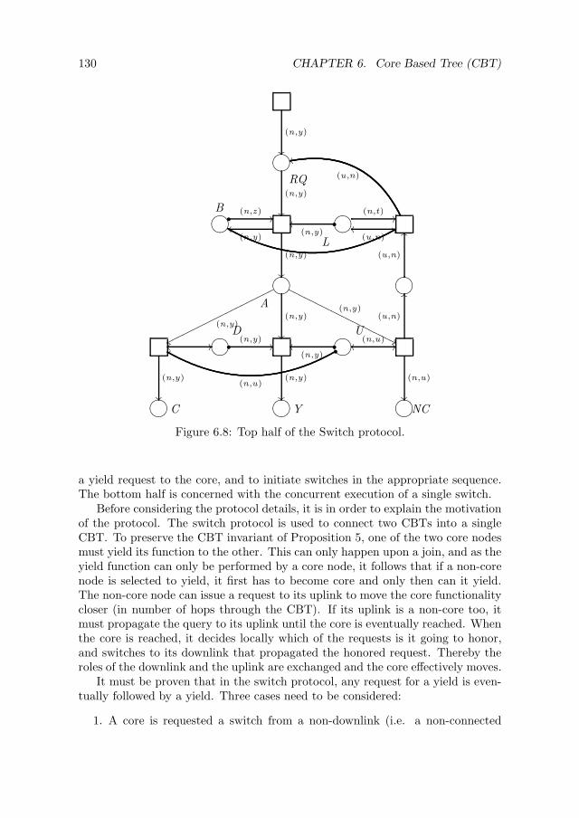
130 CHAPTER 6. Core Based Tree (CBT)
(n,y)
76540123RQ
(n,y)
76540123B
•(n,z)
//
88
(n,y)
(n,y)oo
76540123L
•(n,y)
oo
(n,t)//
(u,n)
rr
(u,n)oo
76540123A
(n,y)
wwoooooooooooooooooooo
(n,y)
(n,y)
''OOOOOOOOOOOOOOOOOOOO 76540123
(u,n)
OO
(n,y)
oo //76540123D
•(n,y)
//
(n,y)
76540123U
•(n,y)
oo oo(n,u)
//•
(n,u)
ff
(n,u)
(u,n)
OO
76540123 C 76540123 Y 76540123NC
Figure 6.8: Top half of the Switch protocol.
a yield request to the core, and to initiate switches in the appropriate sequence.The bottom half is concerned with the concurrent execution of a single switch.
Before considering the protocol details, it is in order to explain the motivationof the protocol. The switch protocol is used to connect two CBTs into a singleCBT. To preserve the CBT invariant of Proposition 5, one of the two core nodesmust yield its function to the other. This can only happen upon a join, and as theyield function can only be performed by a core node, it follows that if a non-corenode is selected to yield, it first has to become core and only then can it yield.The non-core node can issue a request to its uplink to move the core functionalitycloser (in number of hops through the CBT). If its uplink is a non-core too, itmust propagate the query to its uplink until the core is eventually reached. Whenthe core is reached, it decides locally which of the requests is it going to honor,and switches to its downlink that propagated the honored request. Thereby theroles of the downlink and the uplink are exchanged and the core effectively moves.
It must be proven that in the switch protocol, any request for a yield is even-tually followed by a yield. Three cases need to be considered:
1. A core is requested a switch from a non-downlink (i.e. a non-connected
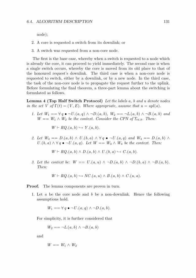
6.4. ALGORITHM DESCRIPTION 131
node);
2. A core is requested a switch from its downlink; or
3. A switch was requested from a non-core node.
The first is the base case, whereby when a switch is requested to a node whichis already the core, it can proceed to yield immediately. The second case is whena single switch occurs, whereby the core is moved from its old place to that ofthe honoured request’s downlink. The third case is when a non-core node isrequested to switch, either by a downlink, or by a new node. In the third case,the task of the non-core node is to propagate the request further to the uplink.Before formulating the final theorem, a three-part lemma about the switching isformulated as follows.
Lemma 4 (Top Half Switch Protocol) Let the labels a, b and u denote nodesin the set V of Γ(t) = (V ,E ). Where appropriate, assume that u = upl(a).
1. Let W1 == ∀ q • ¬U .(a, q) ∧ ¬D .(a, b), W2 == ¬L.(a, b) ∧ ¬B .(a, b) andW == W1 ∧W2 be the context. Consider the CPN of Σ6.8. Then:
W ⊢ RQ .(a, b) → Y .(a, b).
2. Let W3 == D .(a, b) ∧ U .(b, a) ∧ ∀ q • ¬U .(a, q) and W4 == D .(a, b) ∧U .(b, a) ∧ ∀ q • ¬U .(a, q). Let W == W3 ∧W4 be the context. Then:
W ⊢ RQ .(a, b) ∧ D .(a, b) ∧ U .(b, a) → C .(a, b).
3. Let the context be: W == U .(a, u) ∧ ¬D .(a, b) ∧ ¬D .(b, a) ∧ ¬B .(a, b).Then:
W ⊢ RQ .(a, b) → NC .(a, u) ∧ B .(a, b) ∧ C .(u, a).
Proof. The lemma components are proven in turn.
1. Let a be the core node and b be a non-downlink. Hence the followingassumptions hold.
W1 == ∀ q • ¬U .(a, q) ∧ ¬D .(a, b).
For simplicity, it is further considered that
W2 == ¬L.(a, b) ∧ ¬B .(a, b)
and
W == W1 ∧W2

132 CHAPTER 6. Core Based Tree (CBT)
as the assumption. Considering Σ6.8, it is proven:
W ⊢ RQ .(a, b)
RQ .(a, b) ∧W → A.(a, b) ∧W
[¬D .(a, b) ∧ A.(a, b) ∧ ¬U .(a, b)]RQ .(a, b) ∧W → Y .(a, b) ∧W
W ⊢ RQ .(a, b) → Y .(a, b).
2. Consider the case where b is the downlink of a, and a is the core. Thenassume:
W3 == D .(a, b) ∧ U .(b, a) ∧ ∀ q • ¬U .(a, q).
Again for simplicity:
W4 == ∀ q • ¬B .(a, q) ∧ ¬L.(a, q),
so that now the context is:
W == W3 ∧W4.
This yields:
W ⊢ RQ .(a, b) → A.(a, b)
W ⊢ RQ .(a, b) → C .(a, b)
W ⊢ RQ .(a, b) ∧ D .(a, b) ∧ U .(b, a) → C .(a, b),
as required.
3. Consider the case where a and b are not connected, i.e. there is no (a, b) ∈ E ,and a has an uplink u. The context is now:
W == U .(a, u) ∧ ¬D .(a, b) ∧ ¬D .(b, a) ∧ ¬B .(a, b).
Then:
W ⊢ RQ .(a, b) → A.(a, b) ∧ B .(a, b)
[U .(a, u)]W ⊢ RQ .(a, b) → NC .(a, u) ∧W .(u, a) ∧ B .(a, b)
W ⊢ RQ .(a, b) → NC .(a, u) ∧ L.(u, a) ∧ RQ .(u, a) ∧ B .(a, b)
W ⊢ RQ .(a, b) → NC .(a, u) ∧ RQ .(u, a) ∧ B .(a, b).

6.4. ALGORITHM DESCRIPTION 133
Thus, it is seen that a request from a non-downlink b to the node a leaves thenode a busy with processing the request from b (token B .(a, b)), and places it inthe waiting queue for the switch for u (token NC .(a, u)). Applying Item 2 it isobtained:
W ⊢ RQ .(a, b) → NC .(a, u) ∧ RQ .(u, a) ∧ B .(a, b)[ Item 2 ]
W ⊢ RQ .(a, b) → NC .(a, u) ∧ B .(a, b) ∧ C .(u, a),
which is the condition for the entry to the bottom half of the switch protocol.
Lemma 5 (Bottom Half Switch Protocol) Let the labels a, b and u denotenodes in the set V of Γ(t) = (V ,E ). Where appropriate, it is assumed thatu = upl(a). Then:
NC .(a, u) ∧ C .(u, a) ∧ B .(a, b) ∧ D .(u, a) ∧ U .(a, u) →D .(a, u) ∧ U .(u, a).
Proof.
NC .(a, u) ∧ C .(u, a) ∧ B .(a, b) ∧ D .(u, a) ∧ U .(a, u) →M .(T, u, a) ∧ N . 〈rq, u, a, (p, T)〉∧ NC .(a, u) ∧ C .(u, a) ∧ B .(a, b) ∧ B .(u, a) ∧ D .(u, a) ∧ U .(a, u)
NC .(a, u) ∧ C .(u, a) ∧ B .(a, b) ∧ D .(u, a) ∧ U .(a, u) →M .(T, u, a) ∧ [(x ∧ O . 〈rf, a, u, T〉) ∨ (x ∧ P . 〈ac, a, u, T〉 ∧ Q .(T, a, u))]∧ B .(a, b) ∧ B .(u, a) ∧ D .(u, a) ∧ U .(a, u).
The latter inference can be split depending on the value of the predicate x .The only interesting case is when x is false (denoted by x ), when nodes proceedwith the switch. Within the context where x holds, it can be derived:
x ⊢ NC .(a, u) ∧ C .(u, a) ∧ B .(a, b) ∧ D .(u, a) ∧ U .(a, u) →S .(T, u, a) ∧ R. 〈rq, u,n, c, T〉∧ Q .(T, a, u) ∧ B .(a, b) ∧ B .(u, a) ∧ D .(u, a) ∧ U .(a, u)
x ⊢ NC .(a, u) ∧ C .(u, a) ∧ B .(a, b) ∧ D .(u, a) ∧ U .(a, u) →D .(a, u) ∧ U .(u, a).
Considering that the predicate x is external (i.e. unrelated to the decisionprocess), consider only the context x is considered. Considering only that context(i.e. assuming that the switch is not externally invalidated) yields the claim.
Equipped with Lemmata 4 and 5 the main switch theorem can be stated.
Theorem 8 (Switch Theorem) Let a and b be nodes of V , in Γ(t) = (V ,E )such that (a, b) 6∈ E. Let u = upl(a). Then the following holds:
RQ .(a, b) → Y .(a, b) ∧ B .(a, b).

134 CHAPTER 6. Core Based Tree (CBT)
Theorem 8 notes that in any CBT, and any two nodes a and b that do notobviously belong to the same CBT, a request for a join is eventually followed byactivating the yield protocol.
Proof. By induction. The base case is Item 1 of Lemma 4. Adopting aninductive hypothesis from Lemma 4 (items 2 and 3) and Lemma 5, it is seen thatthis happens when u is also the core.
Now consider (with W as in item 3 of Lemma 4):
W ⊢ RQ .(a, b) → RQ .(a, b) ∧ NC .(a.u) ∧ RQ .(u, a) ∧ B .(a, b)
W ⊢ RQ .(a, b) → RQ .(a, b) ∧ NC .(a, u) ∧ C .(u, a) ∧ B .(a, b)[ L. 5 ]
RQ .(a, b) ∧W → RQ .(a, b) ∧ D .(a, u) ∧ U .(u, a) ∧ B .(a, b)[ L., 4it . 1 ]
RQ .(a, b) ∧W → Y .(a, b) ∧ D .(a, u) ∧ U .(u, a) ∧ B .(a, b)
W ⊢ RQ .(a, b) → Y .(a, b) ∧ B .(a, b)
which was to be shown. The remainder of the join is handled by the Yield pro-tocol.
The Yield Protocol
The role of the Yield protocol is to attach two CBTs together.
Theorem 9 (Yield Protocol) Let Γ(t) = (V ,E ) be a connectivity graph at t.Consider the protocol given in Σ6.10, and two nodes a, b ∈ V . Then the followingholds.
R.(b, a) ∧ B .(b, a) ∧ CID .(a, Ca) ∧ CID .(b, Cb) ∧ Y .(b, a)→ (Ca = Cb) ∨ [(Ca 6= Cb) ∧ U .(b, a) ∧ D .(a, b) ∧ CID .(b, Ca)].
Proof. Throughout the proof assume that in Σ6.10 the theorem:
Q .y → A.(y, C) ∧ CID .(coreof (y), C)
holds, i.e. that the node y in question can obtain the component identifier from thecore of its component. This is justified later by Theorem 10. Adopt a shorthand:
W == R.(b, a) ∧ B .(b, a) ∧ CID .(a, Ca ) ∧ CID .(b, Cb) ∧ Y .(b, a).
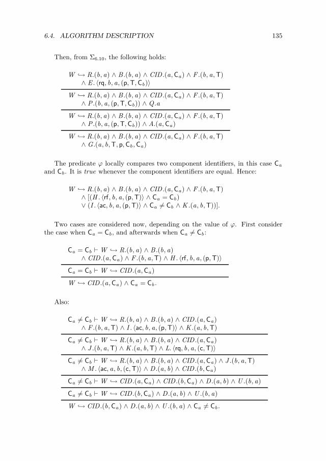
6.4. ALGORITHM DESCRIPTION 135
Then, from Σ6.10, the following holds:
W → R.(b, a) ∧ B .(b, a) ∧ CID .(a, Ca) ∧ F .(b, a, T)∧ E . 〈rq, b, a, (p, T, Cb)〉
W → R.(b, a) ∧ B .(b, a) ∧ CID .(a, Ca) ∧ F .(b, a, T)∧ P .(b, a, (p, T, Cb)) ∧ Q .a
W → R.(b, a) ∧ B .(b, a) ∧ CID .(a, Ca) ∧ F .(b, a, T)∧ P .(b, a, (p, T, Cb)) ∧ A.(a, Ca)
W → R.(b, a) ∧ B .(b, a) ∧ CID .(a, Ca) ∧ F .(b, a, T)∧ G.(a, b, T, p, Cb , Ca)
The predicate ϕ locally compares two component identifiers, in this case Ca
and Cb . It is true whenever the component identifiers are equal. Hence:
W → R.(b, a) ∧ B .(b, a) ∧ CID .(a, Ca) ∧ F .(b, a, T)∧ [(H . 〈rf, b, a, (p, T)〉 ∧ Ca = Cb)∨ (I . 〈ac, b, a, (p, T)〉 ∧ Ca 6= Cb ∧ K .(a, b, T))].
Two cases are considered now, depending on the value of ϕ. First considerthe case when Ca = Cb , and afterwards when Ca 6= Cb :
Ca = Cb ⊢W → R.(b, a) ∧ B .(b, a)∧ CID .(a, Ca ) ∧ F .(b, a, T) ∧ H . 〈rf, b, a, (p, T)〉
Ca = Cb ⊢W → CID .(a, Ca)
W → CID .(a, Ca ) ∧ Ca = Cb .
Also:
Ca 6= Cb ⊢W → R.(b, a) ∧ B .(b, a) ∧ CID .(a, Ca)∧ F .(b, a, T) ∧ I . 〈ac, b, a, (p, T)〉 ∧ K .(a, b, T)
Ca 6= Cb ⊢W → R.(b, a) ∧ B .(b, a) ∧ CID .(a, Ca)∧ J .(b, a, T) ∧ K .(a, b, T) ∧ L. 〈rq, b, a, (c, T)〉
Ca 6= Cb ⊢W → R.(b, a) ∧ B .(b, a) ∧ CID .(a, Ca) ∧ J .(b, a, T)∧ M . 〈ac, a, b, (c, T)〉 ∧ D .(a, b) ∧ CID .(b, Ca)
Ca 6= Cb ⊢W → CID .(a, Ca) ∧ CID .(b, Ca) ∧ D .(a, b) ∧ U .(b, a)
Ca 6= Cb ⊢W → CID .(b, Ca) ∧ D .(a, b) ∧ U .(b, a)
W → CID .(b, Ca) ∧ D .(a, b) ∧ U .(b, a) ∧ Ca 6= Cb .

136 CHAPTER 6. Core Based Tree (CBT)
Joining the above two inferences, the claim of the theorem is obtained.
W → CID .(b, Ca) ∧ D .(a, b)∧ U .(b, a) ∧ Ca 6= Cb
W → CID .(a, Ca ) ∧ Ca = Cb
W → (Ca = Cb) ∨ [(Ca 6= Cb) ∧ U .(b, a)∧ D .(a, b) ∧ CID .(b, Ca)]
Obtaining Component Identifier
Obtaining the component identifiers is used to determine whether two joiningnodes should commit the join transaction. It serves two purposes. First, checks forthe attempts of joins within the same component. Second, it implicitly removesthe cycle in the case of unicycle underlying graph. The Figure 6.11 shows thecomponent identifier algorithm. In Figure 6.10, this protocol component hasbeen compactly represented by the sequence (Q , cq,A) .
Theorem 10 (Component Identifier) Let Γ(t) = (V ,E ) be a connectivitygraph at t. Let T = (V ,U ) be a CBT. Let n and u be arbitrary elementsfrom V , such that upl(n) = u. Then the following holds:
T ⊢ Q .n → A.(n, C) ∧ (CID .(coreof (n), C) ∨ (n 6∈ dom upl ∧ CID .(n, C))).
Theorem 10 says that a component identifier query on the place Q at node ncauses the answer on A with the component identifier C. Then C is either that ofthe core node corresponding to n, or is own identifier if n is the core.Proof. By induction. It is required to establish that the following hold. Afterproving each step, all are assembled into the final proof.
1. Base case. For the base case assume n is the unique core node, i.e. n 6∈dom upl . Then:
T ,n 6∈ dom upl ⊢ Q .n → A.(coreof (n), C) ∧ CID .(n, C).
2. Inductive Hypothesis. The query in the uplink causes an answer in theuplink.
T ⊢ PQ .(u,P , r) → AQ .(u,P , C) ∧ CID .(coreof (u), C).
3. Inductive Step. The inductive step consists of three sub-parts: the upwardpropagation, the downward propagation and finally the answer.
T ,n ∈ dom upl ⊢ Q .n → PQ .(u,P ∪ n, r) ∧ PQ .(n,Q ∪ n, q)
T ,n ∈ dom upl ⊢ AQ .(u,P ∪ n, C) ∧ PQ .(n,Q , q) → AQ .(n,Q , C)
T ,n ∈ dom upl ⊢ AQ .(n,P ∪ n, C) → A.(n, C).

6.4. ALGORITHM DESCRIPTION 137
Each of the above items is proven in turn. For the base case assume CID .(u, C).From Σ6.11, it is immediate that:
Q .n → R.(n,n) →a︷ ︸︸ ︷
PQ(n, n, r) → AQ .(n, n, C) → A.(n, C)
[CID .(n, C)]Q .n → A.(n, C) ∧ CID .(n, C).
Also:
T ,n 6∈ domupl ⊢ Q .n → A.(n, C) → AQ .(n, n, C) → A.(n, C).
For the inductive hypothesis, note first that the element a from the abovederivation establishes a case in which the inductive hypothesis holds. Thus, thehypothesis is valid.
For the upward propagation the following derivation holds:
Q .n → PQ .(n,P ∪ n, r)
[u = upl(n)⇒ U .(n, u)]Q .n → PQ .(n,P ∪ n, r) ∧ U .(n, u)
PQ .(n,P , r) ∧ PQ .(u,Q , q)∧ U .(n, u)⇒ PQ .(u,Q ∪ n, q)
[PQ .(u,Q , q)]Q .n → PQ .(n,P ∪ n, r)
[u = upl(n)⇒ U .(n, u)]Q .n → PQ .(n,P ∪ n, r)∧ PQ .(u,Q ∪ n,min(q, r))∧ U .(n, u)
[p ∧ q ⇒ q, t := min(q, r)]Q .n → PQ .(n,P ∪ n, r) ∧ PQ .(u,Q ∪ n, t).
For the answer:
T ,n ∈ domupl ⊢ AQ .(n,P ∪ n, C) → A.(n, C)
proceed by induction on #P :
1. Base case. If #P = 0, from Σ6.11 the following is available immediately:
AQ .(n, n, C)
[AQ .(n, n, C′′) → A.(n, C′′)]AQ .(n, n, C) → A.(n, C)
2. Inductive Hypothesis. Assume that for all #P = k − 1 the theorem holds.

138 CHAPTER 6. Core Based Tree (CBT)
3. Inductive Step.
AQ .(n,P ∪ n, C)[ upw. prop. ]
AQ .(n,P ∪ n, C) → ∃ y • AQ .(n,R ∪ y,n, C)∧ PQ .(y,S , t)
[ by trans. d ]AQ .(n,P ∪ n, C) → AQ .(n,R ∪ n, C) ∧ AQ .(y,Q , C)
[ p ∧ q ⇒ p ]AQ .(n,P ∪ n, C) → AQ .(n,R ∪ n, C)
[ ind. hyp. ]AQ .(n,P ∪ n, C) → A.(n, C).
The proof components can now be assembled.
Q .n → PQ(u,P ∪ n, r) ∧ PQ .(n,Q ∪ n, q)
Q .n → AQ .(u,P ∪ n, C) ∧ CID .(coreof (u), C) ∧ PQ .(n,Q ∪ n, q)
Q .n → AQ .(n,Q ∪ n, C) ∧ CID .(coreof (u), C)
Q .n → A.(n, C) ∧ CID .(coreof (u), C)
Q .n → A.(n, C) ∧ CID .(coreof (n), C).
From the base case and the inductive proof, as required:
T ⊢ Q .n → A.(n, C) ∧ CID .(coreof (n), C) ∧ n ∈ domupl
T ⊢ Q .n → A.(n, C) ∧ CID .(coreof (n), C) ∧ n 6∈ domupl
T ⊢ Q .n → A.(n, C) ∧ (CID .(n, C) ∨ (n 6∈ dom upl ∧ CID .(n, C))).
6.5 Performance
Two figures of merit are of interest for the performance of the CBT constructionand maintenance algorithm. They are the stretch (the maximum path lengthbetween the nodes) of the constructed graph and the message complexity of theused protocol. The message complexity is expressed in terms of the number ofthe expected number of core switches needed to make a CBT with n nodes, as thenumber of messages per each core switch is constant. The stretch of a CBT is up-per bounded by O(nc), and the message complexity by O(n), where c = log2 3−1.In the analysis some simplifying assumptions are made. First, it is assumed thatat some point in time, the maximal CBT is constructed. In deployment, the CBTconstruction never finishes as long as there are changes in the network. Instead,it continuously repairs the CBT so that only a maximal one remains, providedthat this is allowed by the network dynamics. Second, the concurrent requests tojoin two components, coming from different pairs of nodes, as well as the cycle

6.5. PERFORMANCE 139
breaking are all neglected. This is because the number of concurrent requestsdoes not change the order of the number of switches required, although it doesalter the constant. Furthermore, the number of concurrent requests depends onthe number of nodes in different components that come into contact, a parameteroutside of the scope of this analysis.
The following lemma is needed to prove complexity claims so it is stated first,before the claims and proofs themselves.
Lemma 6 Let f and g be functions of a positive integer k, defined as:
1. f (k) = 1/2 + 3/2 f (⌈k/2⌉), with f (1) = 0;
2. g(k) = ⌈k/2⌉c + 2g(⌈k/2⌉), with g(1) = 0.
Then, f (k) = O(kc) and g(k) = O(k), where c = log2 3− 1.
Proof. For both items, consider only k = 2p for some integer p (otherwisereplace k by 2⌈log2 k⌉ and proceed).
For Item 1, expand f recursively to obtain:
f (k) = 1/2
p−1∑
l=0
(3/2)l = (3/2)log2 n − 1 = O(nc).
For Item 2, expand g recursively to obtain:
g(k) =
p−1∑
l=0
2l · 2(p−l−1)c = 2c(p−1) · [2(1−c)p − 1]/(21−c − 1) = O(2p) = O(k).
The expected stretch of a graph constructed by the CBT algorithm is nowcomputed. Let T be a CBT constructed by our CBT algorithm, and let #Tbe the number of vertices in T . The CBT T was constructed by concurrentapplications of the CBT construction and maintenance algorithm, and T itselfwas obtained by joining together two non-maximal CBTs, say U and W , byadopting an uplink between two nodes x ′ ∈ U and y ′ ∈ W . For x and y twonodes in T , denote as hT (x , y) the hop count of the only path between x and yin T .
Theorem 11 The expected stretch of the CBT T, with #T nodes is O(#T c).
Proof. The mean hop count lT in T is lT = #T−2 ·∑x ,y∈T hT (x , y). Also letL#T = E [lT ] for a CBT T with #T nodes.
Separating over hopcounts in U and W :
lT = #T−2
∑
x ,y∈U
hU (x , y) +∑
x ,y∈W
hW (x , y)
+ 2
∑
x∈U ,y∈W
hU (x , x ′) + 1 + hW (y, y ′)
. (6.9)

140 CHAPTER 6. Core Based Tree (CBT)
Taking the expectation of the hop count (over all the possible graphs T , andalso all components U and W ), and by linearity of expectation:
L#T = #T−2(#U 2L#U + #W 2L#W + 2#U #W
+ 2#U #WL#W + 2#U #WL#U ). (6.10)
As #T = #U + #W , and #U , #W > 0, #U #W /#T 2 ≤ 1/4, hencerewriting Eq. (6.10):
L#T ≤ 1/2 +#UL#U + #WL#W
#T+
1
4(L#U + L#W )
≤ 1/2 + 3/2 max(L#U ,L#W ), (6.11)
where Eq. (6.11) holds over any partition of T to U and W . Hence it must alsohold for max (L#U ,L#W ) = L⌈#T/2⌉. Applying Item 1 of Lemma 6 to the righthand side of Eq. (6.11) for #U = ⌈#T/2⌉ finishes the proof.
Theorem 12 The expected number of core switches needed to construct a CBTT with #T nodes is O(#T ).
Proof. Let M#T be the expected number of switches to construct a CBT T byconnecting the smaller CBTs U and W . Total expected number of switches equalsthe expected number of switches used to connect U and W plus the expectednumber of switches to construct both U and W . Thus the recursive expressionholds:
M#T = 1/2(L#U + L#W ) + M#U + M#W , (6.12)
where the first component is due to the uniform random choice of the componentwhose core executes the yield. As M#T is nondecreasing, assume #U = ⌈#T/2⌉to get:
M#T ≤ L⌈#T/2⌉ + 2M⌈#T/2⌉ = O(#T ). (6.13)
The last equality, due to Item 2 of Lemma 6, completes the proof.
6.6 Summary
In this Chapter, we presented a distributed data structure used for service de-scription forwarding, useful in distributed systems operating in the MANET en-vironment. One must bear in mind that the CBT has been designed for MANETs,where each node has a relatively small number of neighbours and where it is typ-ically difficult or not profitable to keep extensive records of the nodes far away inthe network. This use case is hence different from the peer-to-peer networks whichuse the Internet. In peer-to-peer networks all pairs of neighbours can communi-cate and the problem is to find and use only the efficient number of connections.In MANET however, each node has only a few connections and the problem is to

6.6. SUMMARY 141
inform the further nodes well by forwarding the right amount of soft state. TheCBT is designed to achieve this.
We described the CBT structure, then gave detailed formal account how itis constructed and maintained at runtime and discussed its complexity. We pre-sented the algorithm that uses the CBT structure to propagate the service de-scriptions. We addressed the concern of service description distribution strategy,with a distributed structure which is flat, requiring no dedicated nodes to oper-ate, and requiring no preconfiguration. This is in contrast to service distributionschemes which use a backbone (as discussed in Section 6.1), where role divisionsamong nodes are implicit for the backbone nodes. Instead, each node in theCBT takes an equivalent role in the distribution, and due to the core mobility,is equally likely to become the core node. We do not consider the existence ofthe core node the departure from the flat distribution structure. This is becausethe core performs no special functions, except that it is the node to which all theuplinks point to.
The important property of the core’s existence is that it guarantees that allcompatible producer and consumer summaries are found. An interesting propertyof the obtained CBT structure is that its stretch is sub-linear with respect to thenumber of nodes involved in the structure. This means that the distance betweennodes in the CBT grows slowly with the size of the CBT itself, thus enablingfast operation of the CBT and the appropriate matching algorithms. It is alsoimportant to note the good scalability of the CBT in terms of the required numberof core motions. This because each core motion includes the transfer of the servicedescriptions, which needs to be kept at a minimum. There are some drawbacksto the CBT scheme which need consideration when the cost and benefits of CBTdeployment are estimated. First and foremost, the CBT requires an addressingscheme which is different to what is usually used on the Internet. However, thisis necessary as the internet type addresses do not work in a MANET. Second, itrequires knowledge of, and manipulation with the service descriptions, restrictingthe applicability of the CBT to use cases where service descriptions can be castinto the appropriate dataspace form. While this is a concern in the general case,for well defined tasks (e.g. those described by CPNs themselves) the servicedescriptions are known well enough.

142 CHAPTER 6. Core Based Tree (CBT)
(u,n)
(n,u)
76540123 C
(u,n)
76540123NC
(n,u)
(n,u)
**
****
****
****
****
****
(T,u,n)
〈rq,u,n,(p,T)〉
''PPPPPPPPPPPPPPP
76540123 M
(T,u,n)
(T,u,n)
76540123N
@@@
@@@@
@
''PPPPPPPPPPPPPPP
x
〈rf,n,u,T〉wwnnnnnnnnnnnnnnn x
〈ac,n,u,T〉wwnnnnnnnnnnnnnnn
(T,n,u,f (n))
76540123O
〈rf,u,n,T〉wwnnnnnnnnnnnnnnn
76540123P
〈ac,u,n,T〉wwnnnnnnnnnnnnnnn
(T,u,n)
〈rq,u,n,(c,T)〉
''PPPPPPPPPPPPPPP 76540123 Q
76540123 S
76540123 R
@@
@@@@
@@
〈ac,u,n,T〉wwnnnnnnnnnnnnnnn
(u,n)
76540123
~~~~~~
~~~~
(u,n)
76540123 B
(u,n)>>~~~~~~~~
(u,n)
OO
76540123 U
(u,n)
>>~~~~~~~~~~~~~~~~~~~~~~~~~~~~~~ 76540123 D
(u,n)
``@@@@@@@@
Figure 6.9: Bottom half of the Switch protocol.

6.6. SUMMARY 143
76540123 Y(n,y)
76540123CID
(n,C′)//〈rq,n,y,(p,T,C′)〉
//
(n,y,T)
76540123E
//
(y,n,(p,T,C′))
y
??
????
??
76540123 P
76540123 Q
y
cq
(y,C)
76540123 A
(y,n,T,p,C,C′)76540123 F
76540123 G
??
????
??
ϕ
〈rf,y,n,(p,T)〉
wwoooooooooooooo ϕ
ϕ ≡ C = C′
〈ac,y,n,(p,T)〉wwoooooooooooooo
(y,n,T)
ww
76540123 H
wwoooooooooooooo76540123 I
wwoooooooooooooo
(n,y,T)
〈rq,n,y,(c,T)〉
''OOOOOOOOOOOOOO 76540123 K
76540123 J
76540123L
//
〈ac,y,n,(c,T)〉wwoooooooooooooo
(y,n)
(y,C′)//76540123 CID
(y,C)oo
76540123 M
(n,y)
??
????
??
76540123 R
(n,y)
OO
(n,y)
?? 76540123 B
(n,y)
SS''''''''''''''''''''''''''''
OO
76540123 U 76540123 D
Figure 6.10: The Yield protocol.

144 CHAPTER 6. Core Based Tree (CBT)
76540123 Q
n
(n,n)
76540123 R
(n,n)
(n,n)
??
????
????
????
??
(n,n,n)
??
????
????
????
??
(n,P∪n,min P∪n)
(u,Q∪n,min P∪Q∪n)//
OO
(n,u)
76540123 PQ•
(n,P ,q)
__????????????????
(n,P ,q)
??
(n,P ,q),(u,Q,r)oo
(n,P ,q)
(y,Q,r):y∈P
//
////
////
////
////
////
////
/
76540123U
•(n,u)
//
(n,P ,C)
76540123CID
(n,C)
??
C
??
????
????
????
??76540123AQ
(n,P ,(n,C))//
(n,n,C′′)
(n,∅,C)
??
????
????
????
??d
(n,P\y,C),(y,Q,C)oo
(n,C′′)
(n,C′′)
__????????????????''
C
ggOOOOOOOOOOOOOOOOOOOOOOOOOOO
76540123 A
Figure 6.11: The Yield protocol component query.

Chapter 7
The Execution Model
In this Chapter, we lay out the model for executing distributed programs withinthe Distributed Workflow Execution Architecture for Mobile (DWEAM) con-text. The programs are described by workflows represented with CPNs. In theDWEAM context, the execution of distributed programs reduces to ensuring thatthe progress property holds in face of the node and network volatility. Providedthat the progress property holds, additional safety requirements must be fulfilledso that the semantics of the program execution is equivalent to that given by itsworkflow description, under arbitrary workflow element instantiation.
The workflow elements, i.e. the places and transitions are instantiated onmultiple nodes. There is no restriction on the instatiation cardinality for theworkflow elements. Any token on a given place can be instantiated multiple timesat disparate nodes. Transitions can be similarly instantiated on multiple nodes.
7.1 Introduction
The foundation of DWEAM’s execution model is in the distinction between thedescription of a program (hence: a workflow) and its instantiation (hence: theallocation of procedures to computing elements and the location of objects rep-resenting tokens). This separation may appear a self-evident fact that buys usnothing when we want to understand distributed systems. However, the distinc-tion is in fact important. It is disregarded more often than not, and this becomesobvious if we take a look at the contemporary distributed programs and how themissing distinction hinders the distributed applications.
Looking at the client-server model for communication, which is ubiquitousin todays Internet, we can observe that the above statement is indeed true. Aprime example is given by the common scenario where a user is requesting a webpage from a remote server, through the web browser client. We can consider thecontents of a web page as being some sort of a remote object. The fact that theweb page is usually delivered in a markup language such as Hypertext Markup
145

146 CHAPTER 7. THE EXECUTION MODEL
Language (HTML) is not relevant as it has to do only about the representationof the object offered in response to a query. The representation itself can evenbe the left to the client’s preference. Regardless, the method used to locate theobject is standardized. It is through the URL addressing scheme, which uniquelyidentifies every object accessible from the Internet.
Example 12 Any user of the Internet can request the object whose content isgiven by the URL http:// cobalt.et. tudelft.nl/ ~filip/index.html . Inresponse to the request, the user is delivered the contents of the author’s homepage.
An inherent part of the URL is the Fully Qualified Domain Name (FQDN)of the computer cobalt.et.tudelft.nl, the computer at whose disks the homepage physically resides. If for some reason cobalt is inaccessible, so is the homepage, along with any other objects cobalt hosts. We can conclude that theexistence of the home page object depends on the instantiation at the particularhost, as far as the rest of the Internet is concerned.
If the data objects were decoupled from their instantiations, such an outagewould never have to occur. Unfortunately, since the host-object coupling wasdisregarded in Example 12, the practice dictates we are forced to worry aboutthe well-being of a particular machine, so that the object remains accessible. Ide-ally, the object exists in a data space which is detached from the embodimentand the user’s query for the object should retrieve it regardless of the state theembodiments of the object assume. In thinking about computer programs, weshould worry about the data and the procedures, and not about the machineitself. This point was well conveyed by H. Abelson et al. [7], who teach this dis-tinction in the course MIT CS 6.001, “Structure and Interpretation of ComputerPrograms”. They state that computer science is a misnomer as it is neither ascience (for computer science is about procedural knowledge while science dealswith understanding nature through observation) nor it is about computers (inthe same sense as geometry is about declarative knowledge1 and not about rulersand compasses). It follows that in a distributed system, we should ideally notcare where the actual objects we operate on are located. This is not always easyto achieve, as distributed program components can sometimes follow conflictingexecution paths that contend for data. The practical goal of DWEAM is to ob-tain a distributed environment for program execution that takes the decouplingbetween programs and computers as far as reality permits.
7.2 Data Model
The goal of DWEAM is to provide a workflow execution engine that is inde-pendent of the node network location. That includes processing that does not
1The declarative knowledge is the knowledge about what is true. As opposed to the proce-dural, or how-to knowledge, which talks about the actions needed to bring some result about.

7.2. DATA MODEL 147
fundamentally depend on where the tokens are effectively stored. DWEAM canbe thought of as a workflow processing machine designed to operate over widearea networks of Internet scale without regard of the physical node placement.For such a machine we need to look into two mecnahisms:
1. Location-independent data object storage; and
2. Location-independent data object processing.
These mechanisms must be conceived in a way that fully and correctly im-plements the workflow specification given by the system designer. The location-independent mechanisms are in contrast to today’s practice on the Internet, wherelocation-dependent mechanisms such as the URL are almost exclusively used.
A Case for Location-Independent Mechanisms
A significant complication that surfaces in distributed systems is that apart fromsolving computational problems, the distribution management becomes an issue.In the absence of automated mechanisms to handle the distribution issues, thisconcern comprises a significant portion of the program code. It is then natural toreduce this complexity by factoring the distribution management out of the maincode body and promote it into a separate distribution-handling system compo-nent. This step is as important as it is complicated, because it seems difficultto do this factorization so that the connection between the distribution mecha-nism and the application is broken completely. This observation relates to themodel uniformity problem as given by Homburg et al. in [41]. Talking aboutthe communication primitives that make basic distribution possible, they observethat “[Remote Procedure Call (RPC) and other remote call mechanisms] do notprovide solutions to problems that are common to all wide-area systems, suchas replication, data migration and concurrency control. The effect is that eachapplication has to invent an ad-hoc solution.”
At this point it becomes apparent that the factorization cannot work uncondi-tionally, without introducing assumptions about the method used for the programdistribution. One way to handle the distribution issues is location-independentaddressing. It allows one to address a particular resource, typically a data object,through an uniquely assigned handle. The unique handle is typically sampledfrom a large discrete space.
Workflow Design
In the Chapter 2 we presented a toolkit that is used to specify the tasks to beperformed. As far as the workflow designer is concerned, the distributed executionof the worflow is further left entirely to the workflow management.
Specifically, the task of the workflow management is to instantiate enough“worker” nodes to execute the workflow, and to manage the coordination between

148 CHAPTER 7. THE EXECUTION MODEL
the workers so that the result of the instantiated workflow execution correspondsto that intended by the workflow specification. For a fully distributed system,and especially such that aspires to not rely on pre-existing infrastructure, thecontrol of the task distribution must be distributed itself. It cannot be assumedthat the control process is a centralized entity which is somehow exempt from thevolatility of the entire platform. The control itself is implemented in the samevolatile platform as is the instantiated workflow.
We will now review the requisites for content-based addressing which is theonly addressing mode in DWEAM.
Content-based addressing is a way to refer to a data object by specifying aset of conditions that its contents must fulfill. As objects keep internal state, theconditions have to do with the internal object state. The object’s access control(embodied in the access modifiers) can be used to control which parts of the objectstate are accessible for content-based addressing.
Content-based object selection is common practice in various forms. One formis database querying whereby database tables are searched for records with con-tents fulfilling some particular constraint. Various languages exist for specifyingthe data semantic models. Van der Wolf [84] used one of the available such lan-guages, called Object Type Oriented Data (OTO-D) [5] for the data modeling.
Example 13 (Content Based Query in OTO-D) Selecting a design compo-nent, from [84], page 77:
GET ToolRun ITS Used Opts, Designer, Start Date WHERE ToolITS ToolName = ’Dracula’ AND Start Date ≥ 921027
In the Example 13, in effect a content-based address is formed from the query,and expressed in a semantic database specification language called OTO-D2. Theaddress consists of the composition of two operations: the selection, wherebyonly the objects fulfilling a particular conditions are considered, and projectionwhereby only the relevant fields are selected from all the available ones in themulti-field objects. In the example, the address considers the objects of classToolRun, projecting them to their three attributes, Used Opts , Designer , andStart Date, but only such that the Tool attribute equals to a character string“Dracula” (where Dracula is the name of a toolchain component), and the startdate greater than “921027”.
One must note that the filed matching in the given examples is purely onthe syntactic level. The semantics of the object is defined externally by the datamodel designer. It is the designer who specifies that the string “ToolName” mustcontain the sequence of character corresponding to a particular executable filename, of a program used to manipulate the object. To peruse the object in a
2The OTO-D would in the modern times probably be replaced by some Extensible MarkupLanguage (XML)-based suite of a document type definition and a XML parser, or by a graphicallanguage such as the UML.

7.2. DATA MODEL 149
consistent way across computer systems, the semantics of the object must beknown on a system-wide level. It is to say that a convention, or a standard isavailable, which sets the meaning of all the used objects. While it is true that dueto the object-oriented approach parts of the object semantics can be captured inthe class methods, using the methods the right way is still an external task, thusensuring that the object (and hence its internal state) fits meaningfully into thebroader system context. System-wide standardization of object semantics seemsso far to be the only practical way to achieve such universal semantics adoption.While work is ongoing to make similar semantic models mappable to one another,the absence of widely acclaimed solutions for this problem in today’s Internet-at-large, and the prevalence of single-standard solutions, e.g. those by the WorldWide Web Consortium (W3C), indicate that standardisation is at least a near,to midterm, way to go. On the other hand, strict standardization and fixing theobject semantics is likely too restrictive for a distributed system. Mandating afixed set of contexts in which a particular object can be referenced goes againstthe idea of a heterogeneous system, where supposedly different and non-foreseenobject uses may (and should) appear.
Further, allowing external-context dependent object manipulation restricts theuse of class methods. Given the context dependence they can only be expectedto change or export the objects context-invariant properties. Hence, we can allowthe objects only to be able to export their internal state (such methods are knownas getters), or import internal state (setters, analogously). By this convention weeffectively dropped all class methods, except for the getters and setters themselves.No expressive power is lost however in comparison to designs that freely uses classmethods for object-specific tasks. This is because such a task could encode onlya single object semantics, which we already argued is not the appropriate wayto handle objects in a distributed system. The decision would not be justifiedin the case where the object semantics was fixed on a system-wide level. In thecase of system-wide agreement, the object manipulation code could be embeddedwithin the object itself in line with the usual Object Oriented (OO) practices,hence eliminating the need for context-sensitive handling. This gives rise to anobject models in which methods to manipulate objects exist separately from theobject state, and resembles the object models used in languages such as Schemeor Lisp.
The getter and setter object methods give a way to examine object state andform queries. The approach used to examine the components of the object state(e.g. what variables are there) is called reflection, and is elaborated on in thefollowing section.
Reflection
In this section we will examine the techniques that are used to inspect the contentsof the objects used to transfer messages between the nodes in DWEAM. Thesetechniques are collectively known as reflection and as such appear for instance

150 CHAPTER 7. THE EXECUTION MODEL
in the mainstream programming languages such as Java and Python. The Javaprogramming language provides a facility named Reflect that provides reflectionservices. Python makes a dictionary available for each object created, containingthe detail account of the object internals.
Reflection allows a program routine to inspect the contents of an object byrequesting the values stored within the fields of the object, or to obtain the in-formation about the methods that the object class supports as well as their dec-laration. This allows a program to reflect on its own structure, hence the facilityname. The accessible fields are defined in the appropriate object’s class defini-tion, and are also accessible to the program at runtime. The access methodsexist that allow the program to inspect object contents. This account is validfor dynamically typed languages like Java. It also means that, whenever a newclass is created, the reflection capabilities become available by default throughthe reflection mechanism. For statically typed languages like C++, a similar ef-fect is not achievable with the help of the runtime library alone. Special supportfrom toolkits is needed that does not form a part of the C++ standard library.However, there are programmatic ways by which these features can be emulatedwhere appropriate. It is of course convenient if the language itself provides sucha facility. For this reason we confine our exposition to the environments thatsupport reflection natively, with an understanding that extending the reflectionto other environments can imply some extra considerations.
From here onwards we also assume reflection is available throughout the nodesthat participate in the DWEAM system. Reflection provides us with an importantoperator on data objects. It is used to obtain the fields which some object consistsof. In terms of Object-Z, reflection maps an object into a schema by whichthe class of that object is defined. Once obtained, the bindings from the classdefinition can be extracted, allowing the object’s contents to be inspected.
Example 14 (Reflection) Consider a schema defining a class to contain a tem-perature reading for some particular place:
Temperatureid : N
place : seqCHAR
value : R
unit : seqCHAR
and a variable of that class.
t : Temperature
The type of the schema Temperature is 〈| id : N; place : seqCHAR; value :R; unit : seqCHAR |〉 ([78], page 26). The elements of the schema Temperature

7.2. DATA MODEL 151
are bindings of the form: 〈id 1, place ”kitchen”, value 27, unit ”C”〉,hence the following assignment is valid:
t = 〈id 1, place ”kitchen”, value 27, unit ”C”〉
At the same time, the contents of the binding can be reflected as a sequence ofkey-value pairs as follows:
〈name “id”, type “N”〉,〈name “place”, type “seqCHAR”〉,〈name “value”, type “R”〉,〈name “unit”, type “seqCHAR”〉
Dataspace
In the previous chapters, the notion of Dataspace was introduced as an opaquetype. Operations on this opaque type were introduced too. At this point wewill unpack this opaque type and expose its internal structure. We equip it withconcrete content to represent in detail what it means. This is because we will beneeding operations and predicates talking about parts of the Dataspace. Infor-mally, the Dataspace is a supertype that admits all the instances of all variableshaving all possible constructible types. This is of course not a definition in thestrict sense because it gives no clue how “all possible” values of “all possible types”can be obtained. It does not give a clue whether a type with these properties atall exists. We will therefore give a constructive way to build the Dataspace fromthe suitably chosen primitive types and set of chosen constructors that combinethese types into more complex constructs. Such an approach allows us to buildthe Dataspace inductively.
The first step in constructing is the establishment of the basic types. Here,the basic types are considered within the context of the computer system forwhich the Dataspace is implemented. We adopt somewhat platform-dependentbut yet common types for this purpose. The argument in favor of the choice isthat all practical computer platforms have such basic types in one form or other.These types draw their properties from the adopted machine architecture. Forour purpose the exact choice of the basic types is not essential. But we followthe common practice and adopt the integers (Z), the reals (R, represented by afloating point approximation) and the strings (seqCHAR).
Atoms ::= Naturals〈〈Z〉〉 | Reals〈〈R〉〉 | Strings〈〈seqCHAR〉〉
We further define constructors used first to compose aggregate objects fromthe basic ones. The constructors can be used to aggregate the newly obtainedobjects into more complex aggregates. Constructors we consider are sets (i.e. set

152 CHAPTER 7. THE EXECUTION MODEL
types), sequences and new schemes.
[ SchemaDefs ]
Compounds ::= Sets〈〈PCompounds ∪ Atoms〉〉| Sequences〈〈seqCompounds ∪Atoms〉〉| Schemes〈〈SchemaDefs〉〉
The SchemaDefs represents the aggregate schema types. These are eitherschemas with a single element, or schemas obtained by attaching a single schemaelement to a previously existing schema. The single schema has a generic typeidentifier id , which can be specified at construction time, corresponding to thefree choice for the component name. As the only manner to do so we have, forsimplicity, chosen aggregation, i.e.. packing an arbitratry number of state vari-ables into a single schema. Every schema with n > 1 elements can be recursivelydecomposed into a schema containing n − 1 elements and a schema containingprecisely a single element. We don’t consider empty schemas specially.
SchemaDefs ::= SingleSchema〈〈 〈| id : Dataspace |〉[id ]〉〉| MultiSchema〈〈〈| id : Dataspace |〉[id ]× SchemaDefs〉〉
Finally, the Dataspace is obtained from the three above components, complet-ing the specification of the Dataspace.
Dataspace ::= Atoms | Compounds | SchemaDefs .
Cubes and Cube Sets
An important functionality based on Dataspace is the ability to focus on a partic-ular subset. For this we consider the selection operator. It alows us to specify asubset of the Dataspace for which we have a particular interest in, as it providesthe ground upon which the matching algorithm is built later in the text.
By analogy with physical space, each valid binding (i.e. variable instance)for the type Dataspace we call a point. A point of the Dataspace is uniquelydetermined by a binding that assigns an unique value to each component in thecorresponding type schema.
Example 15 (Compound Schema) With reference to the Temperature schemaof Example 14, we can define another schema that contains it.
Readingt : Temperature
humidity : R
This schema is constructed from a single basic type, aggregated with a componentof a previously defined compound type.

7.2. DATA MODEL 153
A point in the Dataspace is then determined by a binding that assigns a uniquevalue to both the components of the schema. The bindings can also be nested, asis used in this case:
〈t 〈id 1, place ”kitchen”, value 27, unit ”C”〉, humidity 0.6〉.
For the data distribution we need to address larger subsets of the Dataspacethan the individual points. These subsets are then used as objects for commonoperations, such as the service discovery. The subsets are obtained by the selectionand projection operations which constrain the values that can be taken on by theindividual Dataspace schema components. For this purpose we consider eachschema component to be a coordinate. A coordinate is a reflection of a schemacomponent available in the code. We introduce the reflection type specifier Type.This type specifier contains the necessary data to uniquely identify the type itrefers to. It is for instance enough that it contains a string representation of thetype name.
[ Type ]
On the other hand, a coordinate is determined by both the variable type andthe name used to identify the respective schema component. Such a designation isneeded because multiple schema components can be of the same type. Therefore,type alone does not suffice to identify the component, whereas the pair of nameand type does.
Name == seq1 CHAR
Hence, a coordinate is given as:
Coordinatename : Name
type : Type
At this point it is necessary to introduce the typeof and reflect pseudo-operators. These pseudo-operators are difficult to express in the Z notation, asit does not support self-referencing. Hence we use the name pseudo-operators,so as to emphasize the divergence from the rules of Z. The two operators willtherefore be introduced through an example, and an informal explanation of theiroperation. This oddity is not problematic in practice however, for as long asthe reflection is in the vocabulary of the used implementation language. As suchlanguages routinely exist (Java being one of them) we consider this an acceptabledeviation from the Z formalism.
Example 16 (Applying reflection) typeof is a pseudo-operator which, fora given instance variable of a particular type, returns as a result the actual type

154 CHAPTER 7. THE EXECUTION MODEL
from which t takes its value. reflect is a pseudo-operator which, given a typereturns a set of bindings to Coordinate objects, with textual representations of thegiven schema elements.
Consider the schema Temperature as given in the Example 14, and the variablet defined to have this type. Then:
typeof t = Temperature
reflect (typeof t) =〈name “id”, type “N”〉,〈name “place”, type “seqCHAR”〉,〈name “value”, type “R”〉,〈name “unit”, type “seqCHAR”〉
Each Coordinate can take on any value from its support type. If we want toconsider only parts of the entire support set (denoted as X ), a constraint can bespecified. The constraint is generic with respect to the support set. Conceptually,for a support set X , a constraint on it is a subset of X .
Constraint [X ] == P X
Encoding the constraint for a generic set X requires the description of all theelements that form the constraint. However, for sets that have a known internalstructure, encoding the constraint can be more efficient and be significantly ac-celerated. For totally ordered sets, for instance, specifying a continuous intervalamounts to the naming of the bounds, which can be encoded to yield a descrip-tion of constant size, provided that the description of each single element fromthe set is constant size itself. As this is often the case in computer systems, wherepractically all elementary data types are either of constant size (e.g. integersand floating point numbers), the constant size encoding assumption is reason-able. Partially ordered sets exibit a similar structure, with the addition that thedescription size depends on the ordering relation. In such cases, multiple elementsmay have to be counted as comprising the bounds.
Example 17 (Constraints) Integer and floating-point intervals, as representedin finite precision in a computer’s memory, can be encoded in constant space byspecifying the upper and lower bounds only with respect to the ordering relation≤ , in interval notation as: [3, 4], or [2.71, 3.14].
String intervals (seqCHAR) can be encoded in a similar way, with the re-spect of the lexicographic ordering. In interval notation, an example thereof is[“aardvaark”, “zebra”].
Specifying a constraint for some coordinate yields a surface. Multiple surfaceson the components of the same type X taken together, comprise a cube. The cubeis a part of the Dataspace where some coordinates are constrained to intervals.These are the basic Dataspace subsets that can be operated on. Set operations on
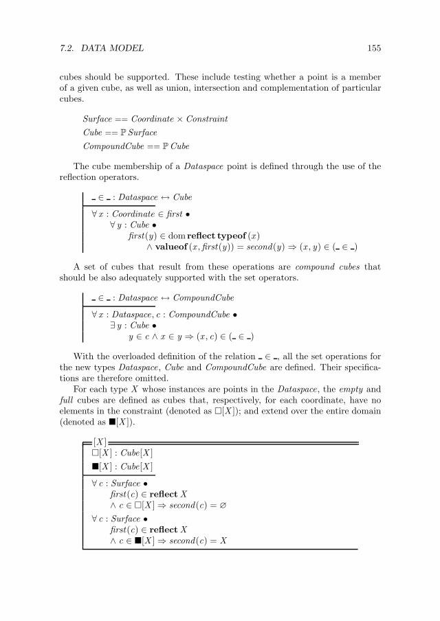
7.2. DATA MODEL 155
cubes should be supported. These include testing whether a point is a memberof a given cube, as well as union, intersection and complementation of particularcubes.
Surface == Coordinate × Constraint
Cube == PSurface
CompoundCube == PCube
The cube membership of a Dataspace point is defined through the use of thereflection operators.
∈ : Dataspace ↔ Cube
∀ x : Coordinate ∈ first •∀ y : Cube •
first(y) ∈ dom reflect typeof (x )∧ valueof (x ,first(y)) = second(y)⇒ (x , y) ∈ ( ∈ )
A set of cubes that result from these operations are compound cubes thatshould be also adequately supported with the set operators.
∈ : Dataspace ↔ CompoundCube
∀ x : Dataspace, c : CompoundCube •∃ y : Cube •
y ∈ c ∧ x ∈ y ⇒ (x , c) ∈ ( ∈ )
With the overloaded definition of the relation ∈ , all the set operations forthe new types Dataspace, Cube and CompoundCube are defined. Their specifica-tions are therefore omitted.
For each type X whose instances are points in the Dataspace, the empty andfull cubes are defined as cubes that, respectively, for each coordinate, have noelements in the constraint (denoted as [X ]); and extend over the entire domain(denoted as [X ]).
[X ][X ] : Cube[X ]
[X ] : Cube[X ]
∀ c : Surface •first(c) ∈ reflect X∧ c ∈ [X ]⇒ second(c) = ∅
∀ c : Surface •first(c) ∈ reflect X∧ c ∈ [X ]⇒ second(c) = X
156 CHAPTER 7. THE EXECUTION MODEL
Following the usual Z conventions, the generic type argument (X in the abovegeneric schema) can be omitted if the type X can be inferred from the context inwhich it is used.
Example 18 (Type Inference) Let a variable t be defined as:
t : Temperature
where Temperature is the type introduced in the Example 14. Then, the expression:
t ∈
is equivalent to:
t ∈ [Temperature]
because typeof (t) ≡ Temperature from the above definition.
Finally, for convenience, to denote the set union (usually ∪ ) and set inter-section operators (usually ∩ ), we use + and · as they make for clearernotation, especially where the operator symbol can be dropped, as is the case inthe expression a · b = ab.
+ == ∪· == ∩
Operations on the Cubes and Cube Sets
Conceptually, once the element containment relation ( ∈ ) is overloaded for theDataspace and the cubes, all the usual set operations are well defined. However,this does not take into account how practical these operations are from a compu-tational point of view. Namely, depending on the order in which the operationsare performed, the size of the compound cubes describing a particular set candiffer, in terms of the number of elements that the respective set has. This trans-lates directly into a varying amount of space used to represent the compound cubein the program runtime environment. Further, more complex descriptions makefor more processing time spent for obtaining a result of a typical set operation.It therefore seems evident that smaller size descriptions are preferred over largerones as compact descriptions save both the processing time and space.
Intersection
When specifying a method to compute the set operations on cubes and cube sets,it is convenient to express these in terms of cubes that themselves do not overlap.Non overlapping cubes allow for the simpler manipulation when determining thesize of the compound cube sets. In other situations, one may opt for the simplest

7.2. DATA MODEL 157
description of the cubes to reduce the required memory footprint3. The simplestway to achieve this is with the intersection of individual Cube objects. Theintersection is defined as a binary operator, taking two arguments, both of thetype Cube.
Let these be x ∈ Cube and y ∈ Cube. The cube intersection computation canbe factored into intersection computation along each of the coordinates. Onlythe coordinates with constraints that are shared between x and y are intersected.The intersection of the two is placed into the resulting cube. The coordinateswhich are not shared are copied from the respective schemas that contain it, intothe resulting schema. Non-shared coordinate constraints (i.e. a coordinate whichis constrained in one cube only and not in the other) are copied into the resultingcube. This is because the coordinates that are not mentioned in the constraintare assumed unconstrained, and the unconstrained coordinate is the identity forthe intersection operator.
· : Cube × Cube → Cube
∀ x , y, z : Cube •(let onlyx == c : Coordinate | c ∈ dom x ∧ c 6∈ dom y;
onlyy == c : Coordinate | c 6∈ dom x ∧ c ∈ dom y;common == c : Coordinate | c ∈ dom x ∧ c ∈ dom y •
z = (onlyx ⊳ x ) ∪ (onlyy ⊳ y)∪(k , c) : Surface | k ∈ common ∧ c = x (k) · y(k))⇔ ((x , y), z ) ∈ ( · )
The intersection of a cube c and a cube set cs is naturally defined by the setcontaining the intersection of c with all the cubes in cs .
· : Cube × CubeSet → CubeSet
∀ c : Cube, cs , r : CubeSet •r = q : Cube | ∃ s : Cube • s ∈ r ∧ q = s · c⇔ (c, cs) 7→ r ∈ ( · )
Finally, two cube sets are intersected by computing element-wise intersections.These are easily expressible in terms of the previously overloaded operators.
· : CubeSet × CubeSet → CubeSet
∀ x , y, z : CubeSet •z = ∪
i∈xx · y ⇔ (x , y) 7→ z ∈ ( · )
3A situation is analogous to that between the uncompressed data stream, which is easy toprocess but potentially takes up a lot of storage, and the compressed data stream, which takeslittle storage but cannot be readily operated on.

158 CHAPTER 7. THE EXECUTION MODEL
Union
Union computation is slightly more involved than the intersection computation,as each union operation yields a cube set. Moreover, extra care needs to be takenthat the resulting cube set is disjoint. A union of two cubes x and y, containsthree sets, namely x\y, x · y and y\x . The intersection can be computed usingthe definitions given before, whereas computing \ deserves extra care.
Efficient difference computation has been constructed following the definitionof the sharp operator described by de Micheli (Section 7.3 in [23]) and inventedby Brayton et al [15], and further in Watanabe et al [86]. De Micheli explains thedifference computation in terms of the sharp operator for positional cube notationand strictly binary coordinates. We extend this definition to general types, i.e.types that can be constructed as subtypes of the Dataspace, and that can bereflected into a set of surfaces. We first present the sharp operators as given byde Micheli, and then extend them to handle generalized types.
The cubes of de Micheli are represented in the positional cube notation. Thisis a binary encoding of the constraint, whereby an k -element set is encoded by abinary string literal of length k . A “1” at the position i of the k -element stringdenotes that the element i is included in the constraint. Conversely, a “0” meansthat the element number i is excluded from the constraint.
Example 19 (Positional cube notation) Let the elements of the support setbe 0, 1, and 2. The constraint, expressed in the positional cube notation willtherefore be a 3-digit binary string literal. The string 001 encodes a constraintfor which only the element 2 is included. The string 110 encodes a constraint forwhich elements 0 and 1 are included.
Cubes are encoded as collections of positional cube denoted constraints. Asthe number of coordinates in the de Micheli case is fixed, any cube can be encodedby fixing the order in which the positional cube denoted literals appear, and fixingthe order in which the support set encodings appear.
Example 20 (Cube encoding) Let there be defined three coordinates, respec-tivelly with the three support sets in the order as follows: 0, 1, 2, a, b, c, d andα, β.
A valid encoding of a cube with elements from the set 0, 1, 2× a, b, c, d ×α, β: is:
011 1101 11,
denoting a cube formed by:
1, 2 × a, b, d × α, β.
In the positional cube encoding, each coordinate can be complemented easily,by making a bitwise complement of the corresponding positional cube encoding.

7.2. DATA MODEL 159
For the positional cube encoding 1101 in the Example 20, the complement in thepositional cube notation is 0010. There are two ways to obtain the differencebetween two cubes. The first is by using the sharp operator. Applying the sharpoperator to two cubes a and b, described by their coordinates: a1 a2 . . . an , andb1 b2 . . . bn is given as:
a # b =
a1 · b′1 a2 . . . an
a1 a1 · b′2 . . . an
. . . . . . . . . . . .a1 . . . an · b′n
(7.1)
where the dot-operator ( · ) denotes a bitwise and between the corresponding co-ordinate bit-strings, and the prime operator ( ′) denotes bitwise complementationof the corresponding coordinates. The result of the operation is a set of cubes,with non-empty intersection. A slightly modified sharp operator, the disjointsharp yields the result in terms of the cubes with empty pairwise intersection:
a©# b =
a1 · b′1 a2 . . . an
a1 · b1 a1 · b′2 . . . an
. . . . . . . . . . . .a1 · b1 a2 · b2 . . . an · b′n
(7.2)
All the cubes in a©# b are disjoint as all the cube pairs have at least one field withan empty intersection. The field i (i.e. ai · b′i) has an empty intersection with thefield i of all the other cubes j > i (which is ai · bi).
Example 21 (Sharp operators, [23] page 292) Let us consider the 2D spacedenoted by: U = 11 11. Consider the cube ab with a = 01 01. Let us compute thecomplement of ab by subtracting it from the U with the sharp operation:
11 11 #01 01 =
10 1111 11
(7.3)
The expression forms the complement a′ + b′. (The operator + is used in theunion sense). Using the disjoint sharp operator:
11 11©#01 01 =
10 1101 10
(7.4)
and the result is now a′ + a · b′ which is a disjoint cover.
The operators we use here are derived directly from the # and ©# opera-tors as shown in the Example 21. There exist differences in how the operators areapplied in the case of Dataspace cubes, when compared to the positional cubes.Two issues to overcome to define the sharp operations on the Dataspace are:
1. The ordering of the coordinates is not predetermined; and

160 CHAPTER 7. THE EXECUTION MODEL
2. The universal full cube [Dataspace] is not well-defined, hence expressionslike a′ where a ∈ Cube, and ′ is the complementation operator, is also notwell-defined.
Both issues can be dealt with efficiently, by modifying the usual sense in whichthe set operations are performed on the points in Dataspace, and provided thatthe resulting properties of the operations are sufficient.
As the coordinate ordering on the types from Dataspace is not predetermined,stemming from no imposed ordering to Z schema components, the positional no-tation is not adequate. Hence the coordinate names must be featured explicitlywhen displaying the cubes and operations. The lexicographical coordinate or-dering is introduced artificially (by the function lex to be defined) so that thesharping-off schema becomes applicable. We do not go into the tradeoff of thecoordinate ordering choice, however.
lex : P Coordinate → seqCoordinate
∀ x : PCoordinate; y : seqCoordinate •ran y = x ∧ dom y = 1..#x ⇔ x 7→ y ∈ lex
As the universal full cube [Dataspace] is not well defined, the complemen-tation of a cube is only valid within the type that the cube describes. Thus, acomplement c′ of a cube c representing a subset of the type Cube[Temperature](schema Temperature is defined in the Example 14) is also a subset of
Cube[Temperature],
such that:
〈c, c′〉partitions[Temperature].
Hence the complement also has no intersection with any [X ] when
X 6= Temperature.
This is in contrast to the case of Example 21, where a complement of a given cubeis with respect to some universal cube U . Here, the complement of a cube is onlydefined with respect to the type the cube has been constructed for.
The definitions of the sharp and disjoint-sharp operators in our context isgiven by the following generic schema:

7.2. DATA MODEL 161
[X ,Y ]# : Cube[X ]× Cube[Y ]→ CubeSet
©# : Cube[X ]× Cube[Y ]→ CubeSet
X 6= Y •∀ x : Cube[X ]; y : Cube[Y ] •
# = (x , y) 7→ x©# = (x , y) 7→ x
X = Y •∀ x , y : Cube[X ]; z : Cube[X ] •∀m ∈ [X ]⊕ y •z = [X ]⊕ (x ⊕ (first(m), x (first(m)) · (X \y(first(m)))))⇔ (x , y) 7→ z ∈ #
(letc == lex(reflect X );xc == [X ]⊕ x ;yc == [X ]⊕ y •∀ k ∈ dom c •
(x , y) 7→ ran〈xc(c(1)) · yc(c(1)), . . . ,xc(c(k)) · yc(c(k))′, xc(c(k + 1), . . . ,x (c(#c))〉 ∈ ©# )
With the sharp ( # ) and disjoint sharp ( ©# ) operators defined, the thesharp operation for cube sets can be built, ultimately admitting the union com-putation for cube sets as well.
©# : CubeSet2 → CubeSet
∀ c1 = q11 , q1
2 , . . . q1#c1 : CubeSet ;
c2 = q21 , q2
2 , . . . q2#c2 : CubeSet ;
r : CubeSet •r = q1
1 ©# q21
∪(q11 ©# q2
2 )©#(q11 ©# q2
1 )∪(q1
1 ©# q23 )©#(q1
1 ©# q22 )©#(q1
1 ©# q21 )
...∪(q1
1 ©# q2#c2
)©#[(q11 ©# q2
#c2−1)©# . . .©#(q11 ©# q2
1 )]
∪(q12 ©# q2
1 )©#[∪(q11 ©# q2
#c2)©#(q1
1 ©# q2#c2−1)©# . . .©#(q1
1 ©# q21 )]
...⇔ (c1, c2) 7→ r ∈ ©#
Finally the union computation for the cube sets is concisely defined throughthe use of the disjoint sharp ( ©# ) operator and the cube set intersection operator.

162 CHAPTER 7. THE EXECUTION MODEL
+ : CubeSet2 → CubeSet
∀ x , y, z : CubeSet •z = x©# y + x · y + y©# x ⇔ (x , y) 7→ z ∈ +
As now the operational definition of the union and intersection operators areavailable, we can investigate how these are used for content-based addressing andobject delivery.
Predicates and Summaries
In content-based addressing, the addresses used for the object delivery are speci-fied in forms of predicates that select a point subset of the Dataspace of interestto the communication participants. Typically, the predicates can be encodedcompactly, so that the resulting description is easy to store and manipulate. Forcompact description though, this requires some knowledge of the structure of thealphabet (i.e. objects used) involved in the communication.
In every communication there are two roles: that of a sender and that ofa receiver. In the communication based on the transfer of objects between thesender and the receiver, it is customary to call the sender a producer (as it pro-duces the communicated objects) and the receiver a consumer (as it consumesthe communicated objects). Further, a communication session can have multipleparticipants fulfilling either of the roles. In contrast to the address based com-munication that is the dominant way for message transport in electronic mail, forexample, where one-to-one communication mode is still dominant, the content-based communication has in principle unlimited number of slots for either role.This is of course conditioned on the ability of the producers and the consumersto locate each other in the network.
A simple example of content-based addressing is reflected in two of the old-est Internet-based services. These are the Internet Relay Chat (IRC) and theUsenet services. Interestingly enough, these services with inherrent many-to-many communication ability have lost in popularity with the wide acceptanceof the Internet, despite their potential, in favor of centralized services such asthe World-Wide Web (WWW) and Instant Messaging (IM). The content basedaddressing present in these services are:
1. Data space partitioning. In this method of group communication, the topicsets partition the entire data space. This method is employed by IRC.
2. Data space partitioning with hierarchical refinement. In this method, thetopic sets partition the entire data space, but can themselves be subdividedand partitioned, thus creating a hierarchical topic ordering. This method isemployed by Usenet.
In both IRC and Usenet, the producers and the consumers gather aroundcommon topics (reflected in the notions of IRC channels, and Usenet conferences).

7.3. MATCHING 163
All the participants can equivocally be both the producers and the consumers.In the case of IRC, the topics are funneled in a flat channel-based topic registry.In the case of the Usenet, the topics are organized in a hierarchical fashion. Aparticipant can therefore narrow down to the topic of own interest, by making aseries of subtopic filters that refine the interest until the participant decides thegranularity is appropriate.
Here we investigate a natural extension to the topic filtering methods. Ratherthan imposing a data space partitioning like IRC or hierarchical selection ruleslike Usenet, we require that the participants can choose an arbitrary Dataspacesubset. This is achieved through the use of summaries. The summaries allow acompact description of the Dataspace of interest for the conversation participants.Conceptually the summaries are no more than CubeSets and can be processed assuch.
Summary == CubeSet .
The reason we introduce this new concept atop the existing cube sets, is thatthere are two classes of summaries needed, one for each of the two roles in thecommunication. We therefore distinguish the producer and the consumer sum-maries. The summaries are essential for the service discovery (refer to Chapter 6). The producer and the consumer summaries that have a non-empty intersectionare considered compatible. That is, objects originating at the respective producermust be delivered to the respective consumer. The process that solves the servicediscovery problem is called matching.
7.3 Matching
Matching is a process used to solve the Service Discovery Problem (SDP) (Chap-ter 6). Informally, it consists of looking at the descriptions of the products sup-plied by the producers, the products demanded by the consumers, and findingwhether such descriptions have commonalities. By using matching on all thenodes in the system, and giving guarantees that any producer-consumer pair iscatered to, allows one to verify the solution of the SDP. Matching usually involvesthree parties. These are the aforementioned producers and consumers (henceforththe clients), and an intermediate broker. The broker is a process that posessesenough information to discern whether particular producers and consumers arecompatible. The broker process adds the necessary loose coupling between com-patible clients. The broker can be implemented as a forwarding service (i.e. mul-tiple nodes may delegate the broker role although the producers and consumersare unaware of this). Matching consists of two sub-processes:
1. Match guarantee. A client must locate an appropriate broker to forwardthe summaries to. The broker must guarantee that a complementing client4
4A producer is complementing for a consumer, and vice-versa.

164 CHAPTER 7. THE EXECUTION MODEL
will be found if it exists. We further postulate that the broker must find allthe complementing clients.
2. Match notification. When the match is found, the matching clients must benotified that the match has been made.
Various strategies exist for handling the matching. There does not seem tobe a universal strategy that works well in all the circumstances. There are de-pendencies upon the number of clients requesting assistance from the broker, thenetwork-wise distribution of the nodes, as well as the connectivity in the networkitself. We identify three classes of strategies, as follows.
1. Centralization. In this strategy, there is a single (physical) broker entity towhich all the producers and the consumers connect.
The upside of centralization is the simplicity. There is a single point ofcontact for all the clients, and there is a single place where all the relevantdata is stored, and is available for any pre-processing.
The downside of centralization is that the broker is forcibly becoming abottleneck. Any dip in the quality of service rendered by the broker reflectsimmediately on the system operation. The broker outage means that allmatching service is inaccessible.
2. Forwarding. In this strategy, there are multiple independent but cooperatingbrokers. Every broker accepts clients, and tries to match the clients locally.On success, the clients are notified. On failure, the clients are forwarded toanother broker that may be eligible to help further. The client must thanre-iterate the request with another broker.
The upside of forwarding is its distributed nature. Provided that a clientcan obtain a reasonably current broker list, it becomes increasingly difficultfor the outage to occur, as opposed to the centralization strategy.
The downside of forwarding is that it requires clients to be able to connectto any broker when needed. This condition may be difficult to fulfill if thenetwork does not exibit full connectivity (e.g. when it is proximity-based asis the case in the MANETs), and the broker can forward the client to anypart of the network in principle. Further downside is that the distributionrequires up-to-date forwarding rules fulfilling the match guarantee.
3. Delegation. This is a more elaborate forwarding strategy. Multiple indepen-dent and cooperating brokers exist as in the forwarding strategy. The brokeraccepts the client, tries to match it, and the client is notified if the matchsucceeds. If the match fails, the broker accepts itself to be a client’s dele-gate, and re-issues the client’s query itself, while the client is still pendingthe broker’s reply.
The upside of this approach is the independence of the full network connec-tivity, provided that the up-to-date forwarding rules are maintained.

7.3. MATCHING 165
The downside of the approach is that the forwarding rules are involved, andbecause of the limited connectivity, the number of brokers tends to be large.Ideally, some brokering functionality is present in every node with the accessto the network.
In the wireless network scenario that we consider (see Chapter 5), the dele-gation is a viable strategy, given the limitations on the direct connectivity rangeimposed by the nature of the medium. Hence a forwarding match strategy mustbe formulated that governs the broker operation when delegating the match re-quests. In the next section we propose a strategy built upon the CBT distributedforwarding structure [60], described in detail in the Chapter 6. The CBT-basedstrategy we consider rests on the assumption that a CBT is established betweenthe nodes, and that it is being actively maintained as the connectivity betweenthe nodes changes.
Forwarding Strategy
The forwarding strategy we consider for the brokers is based on the distributedCBT structure. Conformant to the notation given in Chapter 6, we use φp
a andφca to denote producer and consumer summaries for some node a, respectively.
To simplify the notation of Algorithm 1, we use the familiar vector and matrixnotation to represent in compact form the operations on a sequence of summaries.Thus Φp and Φc, both of dimension k × 1 for some integer k , are vectors intowhich mutltiple producer, and consumer summaries are stacked, respectively. Thematching matrix, obtained as the vectorized intersection Φp · ΦcT of dimensionk × k , has a summary intersection in each its entry.
Further, the summary operator S appearing in the Algorithm 1 warrants ex-planation. It takes some summary φ as a parameter, and produces another sum-mary Sφ which contains at least the points that are elements of φ. Hence, thesummary operator may simply return φ, but as will be seen such a situation is notas interesting as the one where S makes approximate summaries, which hopefullyhave a simpler description than the original one.
The Dataspace in this and the sections to follow is an m-dimensional space,where all the coordinates are integers, for simplicity. The support set for theintegers is denoted as M . Hence in this case, we are considering the set Mm ⊆Dataspace, as the upper bound.
Algorithm
Consider an arbitrary CBT. Assume as usual that the dynamics of the CBTchange is slow, once formed.
Consider now some node n in the CBT. Denote its uplink node as u, andthe set of downlink nodes v1, . . . , vk such that n is an uplink for vi , for every1 ≤ i ≤ k . The matching algorithm for the node n is given in the algorithm 1.

166 CHAPTER 7. THE EXECUTION MODEL
Require: Node n. Uplink node u. A set of k downlink nodes vi : 1 ≤ i ≤ k.A vector of product summaries Φp =
[φp
0 φp1 · · · φp
k
]T. A vector of consume
summaries Φc =[φc
0 φc1 · · · φc
k
]T. S, the summarizing operator.
Ensure: An up-to-date matching matrix M = Φp · ΦcT .if any component of Φp or Φc changed then
Recompute M.Compute φp ← SΦp and φc ← SΦc
Send φp and φc to uSend Sφp
i · φcj to i for all j
Send Sφpj · φc
i to i for all jelse if received φp from u then
Compute Sφci · φp and send to i
Compute Sφpi · φc and send to i
else Initialization stepM = [∅]k
end if
Algorithm 1: Matching.
The algorithm collects the summaries from all downlinks. These summariesare indexed with numbers 1 to k , with summary i pertaining to the downlink1 ≤ i ≤ k . The producer and the consumer summaries are kept apart in thevectors Φp and Φc . Node n adds own summaries, φc
0 and φp0 to Φp and Φc
respectively and computes the matching matrix M. An aggregate summary ismade for the uplink by applying the summary operator S. The uplink u alsoperforms matching and delivers the match to n. If n is the core node, no uplinku exists and the corresponding actions are omitted.
Summaries
A producer p forms its summary φpp and propagates it to its uplink, i.e. the node at
which its only outgoing link points to. Likewise a consumer c forms its summaryφcc and propagates to its uplink. Uplinks are obliged to forward these summaries
further, until the core node of the CBT is reached. In CBT, a unique path existsbetween any producer and consumer pair. Hence it is guaranteed that at least atcore node, φp
p and φcc will be present at the same time in the steady state. The
path to the core on which the summaries are propagated is called the thread5.As the core may be located at any node, the expected length of a thread equalsexpected path length of a tree (E [L]). As the path between the producer (p)and the consumer (c) consists of at most two threads, its mean length is 2 E [L].Without further considerations, the nodes closer to the core are more burdened
5Thread is formally defined on page 171.

7.3. MATCHING 167
with summaries than edge nodes, since they must remember summaries publishedby all nodes in their sub-tree.
This number can be reduced if it is observed that overlapping summaries canbe aggregated, i.e. reduced to a summary that covers given summaries [17].
A summary φ1 covers a summary φ2 if it holds φ1 ⊇ φ2. For a summarysequence φ1, . . . φk , an exact summary is formed as φ =
⋃k φk . It can be seen that
φ covers the given sequence. However, for exact matching, the computing cost forthe matching can be prohibitive and it may become the bottleneck in the matchingprocess. A matching heuristic performs approximate matching [91]. It trades offthe computational complexity of exact matching for additional communicationload for handling false positive traffic. Let there be given a summary φ1 ⊂ Mm .A cover φ2 of φ1 is complete if for every point x ∈ Mm , x ∈ φ1 ⇒ x ∈ φ2. Acover is correct if there exists no point x ∈ Mm such that x ∈ φ2 and x 6∈ φ1.Approximate summaries are complete, but incorrect.
Supercube Approximation
As a simplest approximation, consider the supercube approximation. For the givensummaries, the supercube is the smallest cube covering all the summaries. Let ksummaries be given as 〈φ1, . . . φk 〉 and let lki and uki be the lower and the upperbound of the coordinate 1 ≤ i ≤ m respectively. Define the summary operator Sto yield a supercube. I.e. such an operator S takes a sequence of summaries andproduces a new summary as: φ = S(φ1, . . . , φk ) = [mink l1k ,max k u1k ] × · · · ×[mink lmk ,max k umk ].
A trade-off between false positive matches and description complexity exists.Supercubing introduces #(φ−⋃k φk ) points that cause false positive matches. Italso simplifies the description of the k summaries to only one. Thus communicat-ing the description of the summary induces k -fold less traffic per link, and k -foldless processing time at nodes in the respective thread. Consider a node n of theCBT, as in Algorithm 1, and either producer or consumer summary type withoutloss of generality. To reduce the description that covers φ0 up to and includingφk , n can consider the supercube approximation. A partition of the summary setscan be constructed, and each element of the partition approximated by a super-cube. Choice of the partition depends on the amount of false positive traffic thatis allowable. The false positive traffic amount for the node n can be expressed interms of the probability distribution function over the elements of Dataspace.
In particular, let us consider the object traffic at n. Let us assume that therelative frequency for the arrival of each object from Dataspace to n is known.Denote this frequency as f :
f : Dataspace → 0..1∫Dataspace
f (x )dx = 1

168 CHAPTER 7. THE EXECUTION MODEL
The objects that get delivered to n are the members of the aggregate summaryproduced by n from the exact summaries φ0 to φk for some k , whereas only the ex-act
⋃k φk are actually needed. Thus all extra delivered objects are false positives.
Assuming that all the false positive objects are equal size (as they are in our ex-ample), the fraction of false positives is given by: ω =
∫x∈S(φ0,...,φk)\
⋃k
φkf (x )dx .
The node n can only estimate f , using the traffic received up to some time instant.As soon as a supercube approximation gives too high a fraction ω, n splits theset of summaries from the offending supercube in two and constructs a supercubefor each, thus creating a new approximation.
Summary Operations
In this section we analyze the summary operator S in more detail. We haveseen that the matching is possible when S is complete. It can also be read-ily checked that the sizes of the messages exchanged by the nodes in Algo-rithm 1 depend on the efficiency with which the producer and consumer sum-maries are represented. An incorrect, but complete operator S may incur falsepositives in the matching algorithm, so to eliminate false positives, a correctsummary operator is needed. The problem arises with the size of the efficientand exact description of many summaries. Any complete summary operator isacceptable as long as the number of false positives is acceptable. For exam-ple, adopting a summary operator where (∀A ⊆ Mm) S(A) = Mm yields aflooding communication strategy, at the expense of large false positive traffic.
A
Mm
Figure 7.1: The hierarchical approx-imation of a set A (shaded circle).
Here we suggest the hierarchical sum-mary operator represented in Figure 7.1.In the Figure, a set A (represented by ashaded circle) is approximated by disjointsubsets of Mm (solid rectangles), whichform A = SA. The approximation is gov-erned by a parameter ε, specifying the ceil-ing fraction of generated false positive traf-fic (i.e. the fraction of total transferredpoints of Mm as S is only complete). Ap-proximation starts with a trivial summaryoperator (e.g. supercube). If the approx-imation yields more than fraction of ε offalse positive traffic, the operator is refinedby partitioning the range (dashed lines). The process is repeated recursivelly foreach member of the partition until a sufficiently detailed approximation is found.
Let us now compute the condition for the approximation refinement allow-ing us to find an adequate approximation to an arbitrary set of objects fromDataspace, at node n from the previous section. We already specified that for

7.3. MATCHING 169
simplicity Dataspace ≡ Mm . Consider now a sequence of random variables〈X1,X2, . . . ,Xl〉 for some integer l , representing the object sequence received atnode n. The PDF for each of these variables is equal to fX ≡ f , as before. Nowthe false positive traffic fraction ω is given as:
ω = Pr((X ∈ A,X 6∈ A) ∨ (X 6∈ A,X ∈ A)
)= Pr
(X 6∈ A,X ∈ A
)≤ ε, (7.5)
due to the completeness of S. Expressing Pr(X 6∈ A,X ∈ A
)in terms of the
distribution density fX :
∫
x∈Mm
([x ∈ A]− [x ∈ A]
)fX (x )dx ≤ ε, (7.6)
where [·] denotes an indicator6. Now partition Mm to k approximately equal setsM1, . . .Mk and rewrite Equation (7.6) in terms of the new sets:
∫
x∈Mm
([x ∈ A]− [x ∈ A]
)fX (x )dx =
∑
µ∈Mi :1≤i≤k
Pr (µ)
∫
x∈µ
([x ∈ A]− [x ∈ A]
)fX |µ(x | µ)dx ≤ ε,
(7.7)
where Pr (µ) = # µ /#(Mm) = 1/k , and fX |µ the conditional probability of Xwith respect to the set µ. Finally:
1
k
∑
µ∈Mi :1≤i≤k
∫
x∈µ
([x ∈ µ ·A]− [x ∈ µ ·A]
)fX |µ(x | µ)dx =
=1
k
∑
µ∈Mi :1≤i≤k
[µ ·A 6= ∅]
∫
x∈µ
([x ∈ µ ·A]− [x ∈ µ ·A]
)fX |µ(x | µ)dx ≤ ε,(7.8)
Each of the Mi can be further partitioned as given here, in order to obtain amore precise hierarchical description of A. The hierarchical description of A henceconsists of all the sets Mi and their subdivisions that have a nonempty intersectionwith A (hence also with A). The size of the description is proportional with thenumber of sets in the subdivision (with the proportionality constant the size ofan individual set description in the implementing code). Subtracting left-handsides of Equations (7.6) and (7.8) we see that the two approximations differ by:
1
k
∑
µ∈Mi :1≤i≤k
[µ ·A = ∅]
∫
x∈µ
([x ∈ µ ·A]− [x ∈ µ ·A]
)fX |µ(x | µ)dx (7.9)
6Indicator [P ], where P is some predicate has a value of 1 if the predicate is true and 0otherwise (from [37]).

170 CHAPTER 7. THE EXECUTION MODEL
which is due to the subsets Mi that have an empty intersection with A but havebeen counted in the coarser approximation of Equation (7.6) and left out in therefined one (7.8).
We implemented the straightforward hierarchical summary operator as de-scribed here and in Section 7.3. The set operations operate on integer-only cubes,and the operations have been implemented as an extension of binary value onlymethods described in [23]. The outcome of the summary operator is shown in
0.001
0.01
0.1
1
10
100
1000
10000
0.1 0.2 0.3 0.4 0.5 0.6 0.7 0.8 0.9 1
Rela
tive a
ppro
xim
ation s
et siz
e
False positive traffic
Relative approximation size versus the false positive traffic (Testing dataset)
dim1dim2dim3dim4
0.001
0.01
0.1
1
10
100
1000
10000
0 0.1 0.2 0.3 0.4 0.5 0.6 0.7 0.8 0.9 1
Rela
tive a
ppro
xim
ation s
et siz
e
False positive traffic
Relative approximation size versus the false positive traffic (Random dataset)
dim1dim2dim3dim4
Figure 7.2: The approximation results for a range of common data cube dimen-sions ranging from 1 to 4.
Figure 7.2. The graphs show the relative sizes (up to a constant) of the cubesfrom two different data sets. The first plot is a testing data set, with intersectionsbetween cubes with dimensions from 1 to 4. The second plot shows randomlygenerated data sets with intersection dimensions from 1 to 4. Plots show themaximum allowed false positive traffic on the x-axis. The y-axis shows the size ofthe resulting data set. The unit used is the size of the runtime memory image of asingle data cube7. Plots show a decrease in the description size with the decrease
7As per its current Java implementation. We did not optimize the size of the single data

7.3. MATCHING 171
in the summary precision.
Matching Algorithm
We now consider a matching implementation that takes the properties of the CBTinto account. The basic operation is simple and follows the lines of Algorithm 1to implement a characteristic up-down message passing, common for a wide rangeof algorithms executed on a tree.
Assume that a CBT has been constructed from the graph G. Let b be somenode from V . Let dn(b) be the set of downlinks of b and up(b) the uplink of b, or⊥ if none. For x ∈ p, c (p standing for producer, and c for consumer) introducethe respective summaries. Thus, φx
n is a x -summary of node n. Also, φxn is a
x -summary of the subtree rooted in node n (also denote as x the complementarysummary, i.e. for p, p = c and vice versa). µx
n is a match summary of node n.µ
x
n is a match summary of the subtree rooted in the node n. a → b denotes amessage sent from node a to node b. We formalize the matching requirement asfollows.
Definition 11 (Matching) Let a and b be nodes from G. Let the producersummary of a be given as φa
p , and the consumer summary of b be φbc . A matching
is found for a and b if there exists a node in G which determines that there existsa set X ⊆ φa
pφbc .
Further, the set M , such that X ⊆ M , must be delivered to both a and b.The matching condition determines which producers and consumers need to beconnected together.
Definition 12 (Thread) Let a be a node and there be given a set of iteratedapplications upk (a), for k ≥ 0:
T (a) = a, up(a), up2(a), . . . (7.10)
T (a) is a thread of a.
Lemma 7 The thread of any node a consists of the nodes on the path from a tothe core.
Proof. Let #T (a) be the path length from a to the core node. If #T (a) = 0, theclaim is true by definition. Assume the claim holds for #T (a) = k − 1. Considera for which #T (a) = k . The path from a to the core node leads through upa,so T (a) = a ∪ T [up(a)]. In T (a), a is by definition on the path of the core.Likewise, T [up(a)] are all on the path to the core.
For any node b from a given CBT, the core node is a member of T (a). Thereforefor any two nodes a and b from the CBT, there exists at least one common nodein T (a) and T (b).
cube, although this is possible if needed.

172 CHAPTER 7. THE EXECUTION MODEL
Lemma 8 (Thread intersection) Any two threads have at least one commonnode.
Lemma 8 is a prerequisite for deriving the Matching condition, as it showsthat there exists a node at which matching can be performed. It must be ensuredthat the matching occurs for compatible nodes.
Proposition 7 (The CBT Matching) Let S be a complete summary operator,and let u = up(b). Then the messages:
b → u : φxb
= S[φxb +
∑k∈dn(b) φx
k] (7.11)
∀ k ∈ dn(b) b → k : µx
k = S[φxk· (φx
b + µx
b +∑
l∈dn(b)\k φxl )] (7.12)
guarantee that matching is satisfied for all pairs of compatible producers and con-sumers.
Proof. The operator S is complete. Hence given any set X ⊆ Mm , it must bethat X ⊆ SX . Consider two nodes a and b (a 6= b) with compatible summariesφpa and φc
b . By Lemma 8, there exists a node c such that c ∈ T (a) ∪ T (b). Twocases can be distinguished. First arises when c 6= a and c 6= b. Second ariseswhen c = a or c = b. These cases are similar, so we work the first one out andpick the second one up when appropriate.
Case c 6= a and c 6= b. There is a node ka so that ka ∈ T (a) and up(ka ) = c.Similarly kb exists for b with analogous properties. We prove by induction thatfor any node n ∈ T (a), and any x ∈ p, c it holds that φx
a ⊆ φxn . For n = a,
from Equation (7.11) it holds that:
φxa ⊆ φx
n +∑
k∈dn(n)
φxk⊆ S[φx
n +∑
k∈dn(n)
φxk] = φx
n . (7.13)
hence the base case holds. Assume now that for any sequence of up to l nodesin(a, up(a), . . . , upl−1(a)
)where l < #T a it holds that φx
a ⊆ φxupl−1(a). Using
Equation (7.11), the fact that upl−1(a) ∈ dn[upl (a)], the completeness of S andthe inductive hypothesis:
φxa ⊆ φx
upl−1(a) ⊆φxupl (a) +
∑
k∈dn[upl (a)]
φxk
⊆S[φxupl (a) +
∑
k∈dn[upl (a)]
φxk]
⊆φx
upl (a).
(7.14)
completing the proof that φxa ⊆ φx
n for any n ∈ T (a).Now turn to Equation (7.12). As φp
a and φcb are compatible, a nonempty set
X = φpa ·φc
b exists. We show that X is propagated to both a and b. Consider the

7.3. MATCHING 173
nodes c and ka . Rewriting Equation (7.12) for ka , we get:
X ⊆φp
ka· φc
kb
⊆φp
ka·
∑
l∈dn(c)\ka
φcl
⊆φp
ka· (φc
c + µpc +
∑
l∈dn(c)\ka
φcl )
⊆S[φp
ka· (φc
c + µpc +
∑
l∈dn(c)\ka
φcl )] = µ
p
ka,
(7.15)
and a similar line of reasoning shows that X ⊆ µc
kb. Hence both ka and kb are
notified about a match containing at least X .
It remains to show that both a and b are notified with X . The proof is alsoby induction, the base case thereof already given by Equation 7.15. Let l be suchthat ka = upl (a), and let k ′
a = upl−1(a). By inductive hypothesis, X ⊆ µp
ka.
X ⊆φpk ′a· µp
ka
⊆φp
k ′a
· (φck ′a
+ µp
ka+
∑
l∈dn(c)\ka
φcl )
⊆S[φp
ka· (φc
c + µp
c +∑
l∈dn(c)\ka
φcl )] = µ
p
k ′a
.
(7.16)
Analogous reasoning leads to X ⊆ µpb and we conclude that the matching condi-
tion as per Definition 11 is fulfilled.
Case c = a or c = b. With respect to the former case, either ka or kb (but notboth) do not exist. Without loss of generality, assume c = a. The induction forthe summary φc
b still holds. Match X ⊆ φpa · φc
b is found at a since X ⊆ φckb· φp
a ,
and a is automatically notified of the match by Equation (7.10). To prove that bis notified too, one uses the slightly modified induction given by Equations (7.15)and (7.16). The base case, instead of Equation (7.15), is now:
X ⊆φckb· φp
c
⊆φckb· (φp
c + µca +
∑
l∈dn(a) kb
φpl )
⊆S[φckb· (φp
c + µc
a +∑
l∈dn(a) kb
φpl )] = µ
c
kb,
(7.17)
and the rest of the inductive argument remains the same as before. Also here weconclude that the matching condition is fulfilled, and the proposition holds.

174 CHAPTER 7. THE EXECUTION MODEL
Bloom Filtering for Strings
In this section we refine the matching algorithm for the summaries that explicitlyhave to do with character strings (that is, seqCHARs). In the Section 7.2 theconstraints were presented conceptually as subsets of the support set for a givencoordinate. In general this description is not compact, as for a coordinate withthe support set of k elements, there are 2k possible constraints to encode. Somesupport sets have special structure that can be used to maintain a compact de-scription even if the size of the support set is unlimited. This is precisely the casefor strings, whose support set is infinitely large, and consists of the union of thesets of all character sequences with lengths 0, 1, 2 and so on.
Bloom filters [11] are a device to approximate set membership. A Bloomfilter is a randomized bit array (it uses randomized hash functions) and has somepossibility of yielding a false positive, that is it may posit that an element is in aset, where it is not [61]. The Bloom filter can also be designed to allow for somefixed fraction of false positives. The filter is most efficient if a positive implieslengthy processing, and the “positive” set is only a small fraction of the universalset. Even with false positives, the resulting set for which the lengthy operation isperformed is small.
Bloom Filter Properties
Let there be given a length-m bit sequence B , called the Bloom filter.
B : seq0, 1#B = m
Assume that there are n elements of some set S in total to represent by the bitarray. Initially all the bits in the array are set to 0. A family of k hash functionsis adopted:
[S ]h1, . . . , hk : S → 0..m − 1
It is assumed that the hash functions are independent and produce a randomdistribution of the domain over the range 0..m − 1. The bloom filter is producedfrom the n elements of the set S by computing in turn the values hi(x ) | i ∈ 1..kfor each x ∈ S and setting the bit hi(x ) of the array B to 1. Testing whethersome element q belongs to S amounts to computing T = hi(q) | i ∈ 1..k andchecking that 0 6∈ B(| T |).
The false positive probability is computed considering all the bits in B asindependent. The probability that some bit j in the array is left at 0 after all then elements of S are cached in B is equal to the probability that all the n · k bitsettings set some bit other than j . As there are m bits in total, the probability of
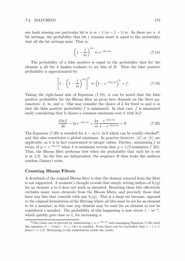
7.3. MATCHING 175
one hash missing one particular bit is is m − 1/m = 1 − 1/m. As there are n · kbit settings, the probability that bit j remains unset is equal to the probabilitythat all the bit settings miss. That is:
(1− 1
m
)kn
≈ e−kn/m . (7.18)
The probability of a false positive is equal to the probability that for theelement q all the k hashes evaluate to set bits of B . Thus the false positiveprobability is approximated by:
[1−
(1− 1
m
)kn]k
≈(1− e−kn/m
)k
= f . (7.19)
Taking the right-hand side of Equation (7.19), it can be noted that the falsepositive probability for the Bloom filter as given here depends on the three pa-rameters: k , m, and n. One may consider the choice of k for fixed m and n sothat the false positive probability f is minimized. In that case, f is minimizedeasily considering that it shares a common minimum over k with ln f :
d ln f
dk= ln e−kn/m +
kn
m
e−kn/m
1− e−kn/m= 0. (7.20)
The Equation (7.20) is satisfied for k = m/n · ln 2 which can be readily checked8,and this also constitutes a global minimum. In practice however, ⌈k⌉ or ⌊k⌋ areapplicable, as k is in fact constrained to integer values. Further, minimizing f interms of p = e−kn/m when k is minimum reveals that p = 1/2 minimizes f [61].Thus, the Bloom filter performs best when the probability that each bit is setis at 1/2. As the bits are independent, the sequence B then looks like uniformrandom (binary) noise.
Counting Bloom Filters
A drawback of the original Bloom filter is that the element removal from the filteris not supported. A moment’s thought reveals that simply setting indices of hi(q)for an element q to 0 does not work as intended. Resetting these bits effectivelyexcludes many more elements from the Bloom filters, and precisely those thathave any bits that coincide with any hi(q). This is a large set because, opposedto the original formulation of the filtering where all bits must be set for an elementto be a member, in this case any element may be reset for an element to not beconsidered a member. The probability of this happening is now about 1 −m−n ,which quickly gets close to 1, for increasing n.
8This claim can be derived by substituting t = e−kn/m and massaging Equation (7.20) untilthe equation (1 − t) ln(1 − t) = t ln t is reached. From there can be concluded that 1 − t = t ,hence t = 1/2. Returning to the substitution yields the result.

176 CHAPTER 7. THE EXECUTION MODEL
To support element removal from the filter, a counting modification is intro-duced to the original filter definition. It replaces each bit of the original filterwith a counter. Adding an element q to a filter increments each counter in theindex hi(q) | 1 ≤ i ≤ k. Removing an element q from a filter decrements eachcounter in the respective index set. Additionally, for space considerations, and forpractical purposes, all counters have a limited range, from 0 to some maximumw . For this reason, the increment and decrement operations are saturating. Thusincrementing w yields w instead of w + 1. Likewise decrementing 0 yields a 0instead of −1. The saturation does not introduce errors in the filter operation.It rather only prevents subsequent removal operations to restore the filter setexactly.
Applying Bloom Filters in the Matching Algorithm
To apply the (counting) Bloom filter for the matching algorithm, one needs tooverload the union and intersection operators for the Bloom filter type. We in-troduce a derivative of a Constraint , which is a counting Bloom filter. The newlydefined Constraint and the related operations given below can be readily pluggedinto the previously defined matching algorithms.
BloomConstraintb : seq 0..m − 1
h1, . . . , hk : seqCHAR → 0..m − 1
#b = k
Testing for membership is achieved by testing for the absence of the element0 in the relational image of the element hash functions.
[X ]∈ : X ↔ BloomConstraint
X 6= seqCHAR •( ∈ ) = ∅
X = seqCHAR •∀ x : X ; y : BloomConstraint •
0 6∈ y.b(| y.hi(x ) | 1 ≤ i ≤ k |)⇔ (x , y) ∈ ( ∈ )
Further, computing union and intersection amounts to maximizing, or mini-mizing the value of the respective counter. The intersections with other types areall empty, while unions are undefined.

7.3. MATCHING 177
+ : BloomConstraint2 → BloomConstraint
· : BloomConstraint2 → BloomConstraint
∀ x , y, z : BloomConstraint •z .b = 〈max (x .b(1), y.b(1)), . . . ,max (x .b(k), y.b(k))〉⇔ (x , y) 7→ z ∈ ( + )
z .b = 〈min(x .b(1), y.b(1)), . . . ,min(x .b(k), y.b(k))〉⇔ (x , y) 7→ z ∈ ( · )
Matching Implementation
In this section we present the implementation of the matching algorithm describedin Section 7.3. The implementation is presented in the form of an appropriateCPN performing steps described in the algorithm description. The CPN revealsthe flow of control for the implementation. The synchronization between theplaces and transitions functions according to the execution rules for the CPN.The account of these rules was given in detail in Chapter 2.
The CPN implementing the matching is shown in the Figure 7.3. It is astraightforward rewrite of the matching algorithm into the CPN form. The Figureshows the places through which the specification and match tokens go within asingle agent. Using the folding technique the same CPN is used to specify thestates of all the nodes in the network. Places U ∗, D∗ and L∗ denote the setof uplinks, downlinks and total links, respectively. The contents of these placesdepends on the environment. The uplink places contain the uplink for every node.The downlink places contain the downlinks for every node. We assume that theexternal mechanism exists that maintains the current view of U ∗ and D∗. Thisfunction is performed by the CBT package (see Chapter 6). Additionally, theassertion L∗ = D∗ ∪ U ∗ holds, as uplinks and downlinks are also links9.
At the top of the CPN of Figure 7.3, one notes three “phantom” transitions:(recvm), (recvs ) and (local). These are the interfaces to the mechanisms thatobtain the remote matches, remote specifications and the local specifications, re-spectively. The remote matches correspond to match messages (see Equation 7.12)obtained from the uplinks k for the node n. The remote specifications correspondto the specifications obtained from downlinks (see Equation 7.11). Finally, thelocal specifications are those published at the local node n, signifying the mes-sages the node n is interested in. The same algorithm operates on both theproducer and the consumer summaries. This is denoted by an upper index x(where x ∈ p, c) of the respective specifications and matches. Hence the givenalgorithm can be understood as two superimposed CPNs, one for x = p, and theother for x = c. These algorithms are not completely independent however, as in
9That is, the implementing classes for downlinks and uplinks are derived from a commonbase class Link.

178 CHAPTER 7. THE EXECUTION MODEL
(recvm)OO
(n,k ,µxk )
(recvs)OO
(n,k ,φx
k)
(local)
OO
(n,φxn)
76540123RM__
(n,k ,µxk )
??
????
????
????
????
?(l,µx
l)
**TTTTTTTTTTTTTTTTTTTTTTTTTTTTTTTTTTTTTTTTTTTTTT 76540123RSOO
(n,d,φx
d)
__
(n,φx
d)
??
????
????
????
????
?
(n,l,µx
l)
''OOOOOOOOOOOOOOOOOOOOOOOOOOOOOOOO 76540123LS??(n,φxn )
OO
(n,φxn)
76540123 L∗
•
(n,l)
CMOO
(n,d,µx
d)
CSOO
(n,φxn)
DEL
76540123U ∗__
(n,u)
??
????
????
????
????
?ww
(n,u)
77oooooooooooooooooooooooooooooooo 76540123 MOO
(n,d,µn
d)
(n,k ,µx
k)
77oooooooooooooooooooooooooooooooo 76540123 SOO
(n,φx
k)
76540123D∗
(n,d)
__???????????????????''
(n,d)
ggOOOOOOOOOOOOOOOOOOOOOOOOOOOOOOOO
76540123SS
•(n,k ,µx
k)
//PM
(n,d,µx
d)
(n,k ,µx
k)
oo PS
(n,u,φxn)
(n,u,φxn)
// //''
(n,u)
ggOOOOOOOOOOOOOOOOOOOOOOOOOOOOOOOO 76540123SM
•oo
76540123RSM
(n,d,µx
d)
76540123RSS
(n,u,φxn)
(sendm) (sends)
Figure 7.3: The CPN showing the matching algorithm.

7.4. THE WORKFLOW MECHANICS 179
the Equation 7.12, the complementing summaries, x and x appear. Still, the twoCPNs are similar enough so as to be folded to a single net, given in Figure 7.3.
The remote and local summaries are collected in the places: Remote Match(RM), Remote Summary (RS), and Local Summary (LS). For each node n re-spectively, these places hold:
1. The matches received from another node k ;
2. The summaries received from another node k ; and
3. The local summary generated at the node n.
The transitions Compute Match (CM) and Compute Summary (CS) respectivelycompute the Equation 7.12 and Equation 7.11. The transition Delete (DEL)removes the stale matches and links when due to the environment influence a link(i.e. a token on Link (L∗)) is lost.
The transitions CM and CS produce the computed Match (M) and Summary(S) tokens which regularly get updated as the specifications on RM, RS and LSchange. Package Match (PM) and Package Summary (PS) package and shipout the readies summaries to Ready Match (RSM) and Ready Summary (RSS).These last tokes are picked up by (sendm) and (sends) and are being transferredto the respective destinations. The destinations are shown in the CPN as d andu respectively. Sent Summary (SS) and Sent Match (SM) maintain a tally of thesummaries already sent and will prevent the sending of new summaries for as longas no changes to the summary occurred since it has been last sent.
The details of the token transfer between (sendx ) and the corresponding(recvx ) are omitted in the presentation of the algorithm. This is because thedialog mechanics has already been described before (e.g. Chapter 6). We there-fore need only to mention a simplified model of the token transfer. The senttriples at (sendx ) for x ∈ m, s always have the form t = (s , d , c), where s isthe source node identifier, d is the destination node identifier and c representsthe content of the transferred summary. At destination (i.e. (recvx )) the sametriples are received as t ′ = (d , s , c). As can be seen, first(t) and first(rest(t)). aretransposed in the received copy t ′ of t .
7.4 The Workflow Mechanics
In the previous sections, we described the data model used for the workflowexecution (Section 7.2), and then we described the mechanism used for matching(Section 7.3). In this section we bring these elements together, describing howthe workflows are maintained by using them and how multiple function instancescoexist when they are physically located at different nodes.
The principal task of the workflow mechanics is to explain the way the datas-pace and subspace selection can be used for flow control in a distributed workflowexecution system. In the Chapter 4 it was shown how inter-related tasks can be

180 CHAPTER 7. THE EXECUTION MODEL
cast into a workflow form by defining guard conditions which determine the neces-sary and sufficient conditions for a task to be activated. It was also demonstratedhow such a specification is cast in terms of a CPN. From there we concluded thata coordinated task set can be expressed in terms of an appropriately annotatedCPN. On the other hand, in the previous Sections it is shown how nodes can usethe constraints to select only the parts of the Dataspace for which they explicitlyexpress an interest in. The underlying thread in this Section is the provision ofa mechanism that can implement a CPN in terms of the operations available onthe Dataspace elements.
Versioning
A part of this task is the assignment of each CPN transition to a node that exe-cutes the corresponding program code, and using the suitable producer-consumersummaries to filter out from the Dataspace the appearance of only the appropri-ate tokens that activate the transitions. Hence, for any CPN an appropriate setof producer-consumer summaries need to be found, selecting only the elementsappropriate for a transition.
The network and node volatility is the main issue. Not only can the nodeoutage prevent a workflow component to be executed (if not handled properly), itcan also cause the system to lose track of the operations that were unfolding. Thenodes in the system must be able to transport the tokens from one to the other,and also make a tally which tokens have been transported already. Hence forall tokens, additional bookkeeping is needed to achieve this. Unfortunately, thisis not achievable through flagging the delivered objects locally. This is becausesuch a marking does not confirm that an object has in fact been delivered andprocessed. Also, as multiple nodes may perform equivalent functions, it is possiblethat due to aliasing, multiple equivalent objects are produced by different nodes.There is no need to deliver multiple such objects (rather only one or two, forinstance). Hence flagging the objects as delivered would produce a system statewhere there exist equivalent objects, of which one is flagged and the rest are not,although all object instances should be considered delivered.
Flagging is not enough to ascertain that some object is delivered. This is be-cause the “deliveredness” of an object can be determined only if the joint statesof both the producers and consumers are considered. Flagging an object as deliv-ered amounts to estimating the state of the consumer as being “object has beenreceived”, and the estimate can of course be wrong. On the other hand, the sum-maries used to determine the compatible interests can remain unchanged whennodes join or leave the CBT. This is because the summaries at a node are alwaysobtained by computing a superset of the summaries forwarded by the neighbours.In both cases, counters are required to denote the situations in which a changeto the object has occurred, without actual change on the object itself (i.e. a new,identical, object instance has become available), or that a summary has changedits composition, without changing the Dataspace subset it refers to.

7.4. THE WORKFLOW MECHANICS 181
The said issues are handled by introducing a version annotation for both theobjects and the summaries themselves. The object and the summary annotationsare somewhat different one from the other. The difference stems from the factthat a summary is unique per CBT, whereas an object can appear accross thenodes in multiple equivalent instances.
Versiontag : R
Object Versioning
For the object versioning, the version tag must fulfill two requirements:
1. Version distinction. Different versions of an object must be such that,clearly, the object history can be derived from the versioning number.
That is, by comparing the version tags of two equivalent objects which arenot the same version, it is possible to determine which one of them is an“earlier” and which one is a “later” version.
2. Object distinction. Different object instances with the same versions needto be distinct from one another, but still be selectable based on the tagidentifier of the associated Version instance.
That is, by comparing the version tags of two equivalent objects with thesame version number, it is possible to establish an ordering based on theversion tag alone.
Adopting a real-numbered version tag handles these two issues. The totalordering with respect to the relation ≤ is established on the set R, hence theversion numbers can be readily compared. As ≤ is also defined on the positiveintegers (the set N), we observe that for the fulfillment of the requirement 1, usingN for this purpose would be just enough.
However, in that case, all the instances of an object with a particular ver-sion tag would become indistinguishable. This would mean that a request for aversioned object would yield potentially many hits, whereas only a single objectwould suffice. For this reason, the following rule is adopted:
Proposition 8 (Object versioning) Let there be given an object o annotatedwith a version v ∈ Version.
1. Version distinction Each object has a Version annotation containing a tag:tag ∈ R. The version of an object o〈v = 〈tag x 〉〉 is therefore given as⌊v .tag⌋.
2. Object distinction Each object instance version is increased by the fraction10
v .tag an unique pseudo-random number from the interval 0..1.
10We use the notation from [37] which introduces the “decimal fraction” operator x bydefining x = x − ⌊x⌋.

182 CHAPTER 7. THE EXECUTION MODEL
Example 22 (Object versioning) Let there be given some object o ∈ Dataspace,with version number 2, and let α and β be the nodes at which the object instancesreside.
The instances are referred to as o ⋄ α and o ⋄ β. When the object o is storedat two nodes α and β, it is assigned a version number 2 increased by a pseudo-random value in the interval 0..1. Hence the object instances would be referred toas:
o ⋄ α〈v = 〈tag 2.1362〉〉and:
o ⋄ β〈v = 〈tag 2.7213〉〉respectively.
The randomized versioning ensures that the ordering between object instancesis preserved, and that the objects remain distinguishable within the same versionnumber. It is therefore possible for the consumers to specify a base version ofsome wanted object o, and to also tune which version range they are interestedin. A consumer interested in a version t of o can start by requesting o with aversion tag that satisfies the predicate ( ≤ 2.1).
If, after some predefined time interval, the consumer does not receive such anobject, it can modify its summary to look for version tags that are the membersof the set defined by the unary predicate ≤ 2.2, and so on, until a suitable objectis found. The consumer can hereby gauge the stream of the delivered objects sothat the network is never overwhelmed with the delivered object copies. Also,eventually the object with version tag 2 will be delivered to it, if it exists.
Proposition 9 (Copying rule) Whenever an object o〈v〉, with v ∈ Version.is copied as a result of any operation (e.g. forwarding), the version annotationv .tag ′ of the copy is set to:
v .tag ′ = ⌊v .tag + 1⌋+ rnd ,
where rnd is a pseudo-random number from the interval 0..1.
In this way, the object instances with an integer version tag ⌊x⌋ get assigneda version number x which is between ⌊x⌋ and ⌊x⌋ + 1. It is straightforward todetermine the object instance version tag distribution in this interval.
Typically, a node requesting an object will try to obtain the most recentversion thereof, and as few redundant copies as possible. Ideally, only one objectinstance will be received. A node can therefore tune its selection policy so thatwith high probability only a single object instance is delivered, and as recent aversion as possible. To achieve this, it is an advisable strategy for a node to tuneits constraint policy so that on average, a single object is delivered to it. Thenode selects the value ⌊x⌋ as the version number. The next step is to choose xthat yields one object as a result.

7.4. THE WORKFLOW MECHANICS 183
Proposition 10 (Versioning rule) Let ⌊x⌋ be the version number of an objecta node has an interest in. Assume that the number of pending objects between⌊x⌋ and ⌊x⌋+ 1 is known to be n. Then the choice of x such that the versionconstraint x = ⌊x⌋+ x yields a single object with the highest probability:
x = 1− e−1/n . (7.21)
Proof. Assume that n object instances are posted in the interval between ⌊x⌋and ⌊x⌋+ 1. For brevity introduce shorthand q == x. Let X (q) be a randomvariable denoting the number of the n objects with the version tag falling between⌊x⌋ and ⌊x⌋+ q.
Then the probability that only a single object falls into this interval is:
Pr (X (q) = 1) = nq(1− q)n−1. (7.22)
The behaviour of Pr (X (q) = 1) on the set [0, 1]× [1, 100] is shown in Figure 7.4.This probability reaches the extremal value at the same point as log Pr (X (q) = 1).
0 0.1 0.2 0.3 0.4 0.5 0.6 0.7 0.8 0.9 1
0 10 20 30 40 50 60 70 80 90 100 0 0.1
0.2 0.3
0.4 0.5
0.6 0.7
0.8 0.9
1
0 0.1 0.2 0.3 0.4 0.5 0.6 0.7 0.8 0.9
1
n*(1-q)(n-1)*q
Figure 7.4: Behaviour of the probability Pr (X (q) = 1) .
d
dnlog Pr (X (q) = 1) =
1
n+ log(1− q) = 0, (7.23)

184 CHAPTER 7. THE EXECUTION MODEL
from where it is concluded that:
q = 1− exp(−1/n)
maximizes the probability that X (q) = 1, which then amounts to:
Pr (X (q) = 1)|q=1−e−1/n = ne−1/n(1 − e−1/n).
Hence, for selecting with highest probability an interval that contains a singleobject, nodes should estimate the number of candidate objects n, and then setthe fraction x to the value given in the Equation 7.21.
As n is typically unknown, we must settle for an estimate for n. The estimatecan be derived as follows, from the past observations of the same version rangefor one particular object instance.
Proposition 11 (Estimating instances) Assume that for r various values ofx being q1 up to qr , the following samples are obtained: n1, n2 up to nr . Thenthe estimate for the total number of objects within the range 0..1 is:
n =1
r
∑
1≤i≤r
ni
qi. (7.24)
Proof. The probability for the realization of the event (n1, . . . ,nr ), where thesamplings of ni are independent for all i is:
Pr (n1, . . . ,nr ) =r∏
i=1
(n
ni
)qni
i (1 − qi)n−ni . (7.25)
The likelihood function is obtained as: L(n1, . . . ,nr ) = log Pr (n1, . . . ,nr ). Differ-entiating L with respect to n:
dL(n1, . . . ,nr )
dn=
d
dn
∑
1≤i≤r
log
(n
ni
)+ ni log qi + (n − ni) log(1− qi) = 0. (7.26)
The log-binomial log(nni
)is expanded, taking into account that
(ab
)= a!
b!(a−b)! for
a ≥ 0, b ≥ 0 and a − b ≥ 0, to yield:
L(n1, . . . ,nr ) =∑
1≤i≤r
∑
1≤j≤n
log j −∑
1≤j≤ni
log j −∑
1≤j≤n−ni
log j
+ ni log qi + (n − ni) log(1− qi).
(7.27)
The sum-logs on the right-hand side of Equation (7.27) are approximated by theStirling formula:
∑
1≤k≤x
log k ≈∫ x
1
log kdk = x log x − x , (7.28)

7.4. THE WORKFLOW MECHANICS 185
to yield the approximation:
L(n1, . . . ,nr ) ≈∑
1≤i≤r
n log n − ni log ni − (n − ni) log(n − ni)
+ ni log qi + (n − ni) log(1− qi).
(7.29)
Differentiating the approximate expression for L from Equation (7.29), oneobtains the condition:
dL(n1, . . . ,nr )
dn= r log n −
∑
1≤i≤r
log(1 − qi) + log(n − ni)
= 0 (7.30)
that reduces to: ∏
1≤i≤r
(1− qi) =∏
1≤i≤r
(1− ni
n
). (7.31)
The Equation (7.31) is satisfied for:
n =ni
qi, for all 1 ≤ i ≤ r . (7.32)
Adding all the expressions n = ni/qi from Equation 7.32 up yields:
rn =∑
1≤i≤r
ni
qi, (7.33)
leading to Equation (7.24).
From Proposition 11 we see how a node can estimate the number of objectinstances, given past observations. Thus obtained estimate for n can then besubstituted into the Equation (7.24) to yield the size of the selection x.
This versioning alone is not enough for the correct selection of the desiredobjects from the neighbouring nodes. As with objects, the summary versionsplay an important role, and we therefore treat their versioning in the followingSection.
Summary Versioning
As with the objects, the summaries delivered between nodes must be versioned.The versions on summaries are required to propagate the changes to the producerand the consumer sets as well as the changes of the summaries themselves.
As an illustration, consider the society given in the Figure 7.5 showing theinteraction between three nodes named α, β and γ. The nodes are represented bycircles, and the summaries reported to uplinks are represented by the annotatedsummaries φ. Figure 7.5 shows a simple scenario in which a new node joins analready existing CBT structure for which a summary φ has already propagated

186 CHAPTER 7. THE EXECUTION MODEL
76540123φ 〈v = 〈tag 1〉〉
α
76540123
??
φ 〈v = 〈tag 1〉〉β 76540123
__??
??
γ
76540123φ 〈v = 〈tag 2〉〉
α
76540123φ 〈v = 〈tag 1〉〉
??β 76540123
__????????
φ 〈v = 〈tag 2〉〉γ
Figure 7.5: The need for summary versioning.
through (left). Incidentally, the node γ contributes a new summary which denotesthe same Dataspace subset as those of the nodes α and β.
Since the summary of γ is also equal to φ, without additional provisions, αwould not need to modify its aggregated summary. But, although not changingthe summary is economic in terms of the bandwidth saved for not transferringan unchanged summary, it also entails that γ will not be delivered any objectspresent on α which have already been delivered for the summary version 1 of φduring the time γ was not included as a consumer.
To do this, however, the node γ must specify a version tag that is higher thanthat present in the uplink. It is not always necessary that γ requests all the objectsfor its particular summary. This depends on whether γ is introduced to take upthe upcoming workload (from the time it joins onwards), or it is introduced totake over the objects posted before it joined the network.
When computing the summaries (according to Proposition 7) in the CBTstructure, the node11 b annotates the resulting summary with a version tag thatis the maximum of all the version tags of the constituting summaries.
Proposition 12 (Versioning summaries) Let b be some node in the CBT.Let dn(b) be the set of its downlinks. Let b compute the summary to be forwardedto u = up(b) according to the Equation (7.11). Additionally, let each summaryφxk
for all k ∈ dn(b), as well as φxb be annotated with the corresponding version
tag. Let these annotations be φxb .v and φx
k.v for all k ∈ dn(b), respectively.
Then the annotation for φxb
is obtained as:
φxb.v =
⟨tag max
[φxb .v .tag,max k∈dn(b) φx
k.v .tag
]⟩(7.34)
From the Equation (7.34) we see that each node b forwards a maximum versiontag of the subordinate summaries along with the summarized tag. This taggingensures that any change in the number of downlinks along a thread12 gets even-tually propagated up a thread, as long as the version tag associated to the changeis the maximum along a thread.
11Refer to Proposition 7 on page 172 for details about the notation.12I.e. those connected by the uplink and downlink relations.

7.4. THE WORKFLOW MECHANICS 187
A similar rule is valid for the match computation. Here the version tag of thecomputed match is again the maximum of the version tags of all the summariesused to compute it.
Proposition 13 (Versioning matches) Let b be some node in the CBT. Letdn(b) be the set of its downlinks. Let b compute the summary to be forwardedto k ∈ dn(b) according to the Equation (7.12). Additionally, let each summaryφxk
for all k ∈ dn(b), as well as the summaries φxb and φx
kbe annotated with
the corresponding version tags. Let these annotations be φxb .v and φx
k.v for all
k ∈ dn(b), respectively.Then the annotation for µ
xk is obtained as:
µx
k .v = 〈tag max [φxk.v .tag, φx
b .v .tag,
µxb .v .tag,max l∈dn(b)\k φx
l.v .tag]〉 (7.35)
The node b of the CBT can therefore specify a version tag through annotatingits client summary, and can observe the effect of putting an annotation into thesummary by testing the version tag on the respective match. Depending on theintended role of the node, the node may want to impose the maximum versiontag for its thread. This happens if the node should collect the objects that hadbeen exported by other nodes in the CBT prior to its activation in the CBT. Ifthe node is included only to continue the work from a certain point onwards, itneed only set its version tag to be equal to that of the current match.
Hence, the strategy for a node that establishes a new connection with an uplinkin its CBT is to select a version tag for the summary higher than the previous onefor the respective match. And the strategy for a node that reinstantes an existingconnection is to set a version tag higher than that of the current match.
With the object and the summary versioning in place, the bookkeeping ofthe object delivery is simple. Per object, a last delivered version tag is kept. Itdenotes the last match version for which an object copy was delivered.
LastDelivered == Version
The delivery is directed by the following simple rule.
Proposition 14 (Delivery rule) Consider an object o〈l = 〈tag l∗〉〉 and amatch µ〈v = 〈tag v∗〉〉. Then the LastDelivered tag of o is updated, and the oforwarded to the owner of µ by:
∆LastDeliveredv∗? : R
tag < v∗? •deliver o for µ.tag ′ = v∗?

188 CHAPTER 7. THE EXECUTION MODEL
As the matches consist of disjoint cubes, there will be at most a single cubeC within the match µ for which o ∈ C . Hence object is delivered only once for asingle node, per each version change that ensures that l∗ < v∗.
Waiting on Multiple Tokens
In Chapter 2 the triggering mechanism for transitions was described. The trig-gering mechanism takes care that each CPN transition (implemented by a nodein the CBT) gets activated if and only if the preconditions for this are fulfilled.The triggering mechanism must also take care that the tokens fulfilling the pre-condition for some transition are processed only once, provided that no versionchanges on these objects have taken place.
In line with the requirement to handle the node volatility13, multiple instanti-ations of the same transition must be supported. By multiple instantiations of asingle transition, we mean multiple nodes which implement functionally identicaltransitions. Supporting multiple instantiations translates into the bookkeepingrequired to direct all the available tokens only to a specified set of receivers. Tounderstand this properly, we take a look at the components that any workflowconsists of, shown in the Figure 7.6.
Depending on the number of the input and output places we distinguish thefollowing CPN basic building blocks:
1. Contract is the building block consisting of a transition t , where #(t) >1, and #(t) ≤ 1 (when #(t) = 0, then t is also a sink). Upon eachactivation, the contract transition reduces the total number of active tokens(as the number of input places is smaller than the number of output places).According to the activation rules from Chapter 2, the token types b and cmust depend on only one of the other tokens (say a). Hence: b = b(a), andc = c(a).
2. Expand is the building block consisting of a transition t , where #(t) ≤ 1,and #(t) > 1 (when #(t) = 0, then t is also a source). Upon eachactivation, expand increases the number of active tokens.
3. Reduce is the building block that consists of a transition t , which producesand consumes tokens from the same place. Such a transition can occurtypically for cumulative operations, arising from say summation.
4. Map is the building block for which #(t) = #(t) = 1. This block con-sumes a single token from the only place in t , and delivers it to the onlyplace in t.
Note that the blocks for which simultaneously #(t) > 1, and #(t) > 1 canbe described by a serial concatenation of an expand block with one contract block,
13See page 10 on node volatility.

7.4. THE WORKFLOW MECHANICS 189
76540123 A
a,,
76540123 B
b
76540123 C
crr
td
76540123 D
(a)
76540123 A
a
tb
c
d
76540123 B 76540123 C 76540123 D
(b)
76540123 A
a
t
b
OO
(c)
76540123 A
a
tb
76540123 B
(d)
Figure 7.6: The basic CPN building blocks. (a) Contract. (b) Expand. (c) Re-duce. (d) Map.
by making the unique post-place of the latter the unique pre-place of the former(see Figure 7.7). The access modes14 are syntactic sugar so there is also no needto show them here explicitly.
When the CPN is implemented, each transition is allocated to some node.To prevent problems relating to volatility, as well as to enhance throughput, thesystem designer would want to allocate multiple instances of the same transitionin different nodes. This gives rise to the need to synchronize the instantiations,so that the activation semantics of the CPN can be honored. For this, somedistributed queuing method for each transition needs to be applied.
Various strategies exist for this [44]. The first option is centralized queueregulation through an unique process, the queue manager. While simple, thisqueuing solution has two important drawbacks:
1. With the increase in the number of queues to manage, the manager ends upwith a high workload. It ultimately becomes a bottleneck.
2. Under network and node volatility, the queue manager also becomes a singlepoint of failure, whose absence prevents the CPN execution.
14The access modes were shown in Chapter 2, on page 31.

190 CHAPTER 7. THE EXECUTION MODEL
76540123 A
a,,
76540123 B
b
76540123 C
crr
td
76540123 D
d
te
f
g
76540123 B 76540123 C 76540123 D
Figure 7.7: Attaching an expand to a contract building block.
The second option is having each producer multicast the state of the tokens itcontains to all the consumers. Again, the simplicity of the scheme is outweighedby the two principal drawbacks:
1. This approach entails a lot of messages for synchronization.
2. Care must be taken that each token offered by a producer is consumed onlyonce in a given context.
A separate issue arises with the contract basic building blocks. A contractbuilding block (call it k) waits on multiple tokens originating from disparatenodes. At the same time, the block k can have multiple instantiations residingon different machines. Upon the delivery of the tokens in the set k it must beensured that all tokens relevant for k are not only delivered to an instance of k ,but also that all tokens of the places from k are delivered to the same instanceof k .
The ideal approach for the synchronization of multiple producer-consumer in-stances forwards the tokens (i.e. the products) so that all the consumer instancesare busy processing the tokens and that some goal function is optimized. Typicalgoal functions are balancing the load on the consumers, maximizing the cumula-tive token throughput, or minimizing the time for processing a single token.
We do not go into the ways the execution is optimized. Here we only treat themechanism with correct token delivery as the only functional requirement. Onthe non-functional side though, the following requirements are important:
1. The avoidance of centralized setups (e.g. the queue manager approach givenabove). This requirement stems from the network volatility assumption. Ina volatile network, it is not possible to employ an effective queue manager,

7.4. THE WORKFLOW MECHANICS 191
since it is as susceptible to volatility as any other process. It thereforeremains a bottleneck for the entire system, regardless of the existence of themultiple instances of the consumers.
2. Proactive handling of the node volatility. This requirement specifies anapproach to handling node volatility before it occurs.
While it is considered an overkill in computer systems with assumed infre-quent fault, it is quite a natural assumption in the communication systems,for instance. As we identified node volatility to be ever-present in DWEAM,proactive handling of node volatility is justified.
Mutual Adjustment Strategy
From the above requirements, the coordination strategy of mutual adjustment [82]between the nodes implementing transition instances is imminent. The mutualadjustment is a coordination strategy used in distributed systems, whereby thesystem components cooperate in managing their own workload, without an ex-ternal supervisor entity. The mutual adjustment strategy employed here is basedon the problem space partitioning concept. This strategy is used given that, dueto the task decomposition into a workflow and the representation by CPN transi-tions, the transition instances apply identical procedures to the tokens in the inputplace. As opposed to the queue manager approach, where the queue manager ex-plicitly decides which worker takes a work item, we adopt an implicit approach,in which no queue manager exists, and the task assignment is randomized.
We introduce a simple mutual adjustment schema based on the assignment ofunique identifiers to points of the Dataspace, and partitioning the identifier spaceamong all the interested transition instances. Trading off top performance forcoordinator-less operation, we obtain a strategy that guarantees eventual progressof the involved tokens, if the processing is feasible (i.e. at least one appropriatetransition and the network connection exist). For this purpose an additionalcoordinate is needed in the Dataspace. We call this coordinate the DSUID . It isused as a mutual adjustment key.
[ DSUID ]
The DSUID is an unique identifier type, from which elements can be drawnrandomly. Further assume for simplicity that each transition of the CPN to beexecuted has been allocated a distinct numeric DSUID too (presumably by thesystem designer).
A straightforward way to implement DSUID is to represent its elements bya sequence of l digits taken in some base b. In practice, b = 2 is usually used(corresponding to using the identifiers encoded in binary), with l an implementa-tion parameter, chosen so that bl is large enough to contain all the objects in the

192 CHAPTER 7. THE EXECUTION MODEL
Dataspace15. An element e ∈ DSUID is sampled from DSUID by generating uni-formly at random each of the l sequence elements. As a result, set of the tokensfrom Dataspace will have DSUID coordinates that also uniformly at random fillthe DSUID space.
To partition the DSUID set and allocate each partition element to some in-stantiation i of a transition t , distinction must be made between instances t ⋄ i foreach i . For this, each node hosting an instance t ⋄ i should choose own identifier,from which the transition identifier can be recovered, and the identity of t ⋄ ican be maintained. Both goals can be achieved with a single identifier, as longas the upper bound on the number of functions and the number of implementinginstances is known.
One can employ a simple idea coming from the coding for telecommunicationsto achieve this goal. The transition instance identifier is built from two compo-nents. The first is fixed, and corresponds to the transition identifier. One canlook at this as a “codeword”. To this codeword, an unique, randomly generatedidentifier is superimposed, by bitwise addition, considering both identifiers as bi-nary numbers. The randomly generated identifier corresponds to random “noise”which is superimposed to a codeword when it is transferred through a communi-cation channel. Well known coding schemes exist (Reed-Solomon, BCH, Turbo,Low Density Parity Check Codes, to name a few) by which the original codewordcan be recovered efficiently from the “noisy” codeword.
In a similar manner, here the effect of noise is simulated, with the goal toobtain unique identifiers, distinct with high probability, but which cluster aroundthe transition codeword, in the sense of some distance measure. A simple measuresuch as Hamming distance16 suffices. From the unique identifiers, the transitioncodeword can be recovered by standard decoding methods. Contrary to the com-munication case where the noise is a feature of the communication medium, theadded noise in our case is under direct control. Care must be taken to make thenoise of low enough power so to not disturb the decoding by introducing spuriouserrors. The random identifiers can be generated completely independently by theimplementing nodes.
Once the instance identifiers are assigned, a simple mutual adjustment strategycan be employed: a produced object is delivered to all different transitions thatconsume it, and within the transition, to the transition instances with DSUIDsclosest to the DSUID of the object itself. The system designer may decide toinstruct the system to deliver the object to c > 1 closest transition instances, thusensuring that the outage of any one single instance does not affect the subsequentavailability of the computation outcome. We arrive at a delivery proximity rule.
15This is easily achieved in practice, as for instance if b = 2 and l = 400, then bl ≈ 2.5 ·10120,generously topping the number of hydrogen atoms in our galaxy.
16Hamming distance between two binary numbers x and y is equal to the number of bitpositions in x and y that have different value.

7.4. THE WORKFLOW MECHANICS 193
Proposition 15 (Delivery Proximity Rule) Objects representing the tokensin the CPN are annotated with a randomly assigned DSUID, as described. In-stances that implement transitions are assigned a randomly generated DSUID asdescribed. The token objects, when produced, are delivered to the c of the trans-action instances which have the c closest DSUIDs to that of the token object.
Multiple Input Tokens
For transitions that expect tokens from at most a single place (such as the mapand expand from Figure 7.6b,d), the mutual adjustment strategy as describedby the previous section can be considered enough to ensure that a transition iseventually delivered the tokens needed for firing.
With multiple tokens, as is the case of the reduce (Figure 7.6a), the mutualadjustment entails a complication: the input tokens, which can originate at un-related nodes, must be delivered to the same transition instance. It means thatthe unrelated tokens must bear the same DSUID , so that the view on the closesttransition instance is the same for all the tokens, and that token DSUIDs must bedelivered to all of them. A possibility for brokering the DSUIDs in such a way isto assign them upstream (in terms of the defining CPN) in a transition commonto all the tokens. The brokering example is given in Figure 7.8.
Such an arrangement implies that, for determining the transition instanceat the minimum-distance from a given object, the instance DSUIDs must beknown. The DSUID information can be readily attached to the producer andconsumer summaries. Each node delivers adds own DSUID to the summary,together with all DSUIDs received from the downlinks. As the only nodes usingthe DSUID data are those at which the transition instances reside, they arethe only ones at which the transition instance DSUIDs need to be kept. Callthe facility in which the transition instance DSUIDs are stored a DSUID table.These tables contain the data about the transition instance DSUIDs and is kept insynchrony with the DSUID labels delivered through the summaries and matches.Unrelated DSUID table instances are not guaranteed to be synchronized, forperformance reasons. Synchronizing the DSUID tables would entail the need fordistributed transactions. Omitting the synchronization leads to a system state inwhich different nodes may hold conflicting DSUID tables.
It can therefore occur that, for some contracting transition t there exist dif-ferent transition instances, at nodes α and β, t ⋄α and t ⋄β respectively, to whichthe related tokens from distinct places from t get delivered, although they shouldhave been delivered to a single instance of t . These tokens trigger the guard oftheir respective transition17 but as they are not present simultaneously at thesame node, the transition t would never get executed. We therefore have twoopposing forces in the token delivery: the delivery proximity rule, stating that for
17See Chapter 2 for the description of the guard in the blackboard-based CPN implementa-tion.

194 CHAPTER 7. THE EXECUTION MODEL
76540123
DSUID generated
ww
76540123
OOO
76540123
OOO
76540123
OOO
76540123
..
76540123
76540123
DSUID used
99
%%
76540123
Figure 7.8: Brokering. The example shows an expand transition that generatesDSUIDs for three separate token streams. The streams are joined by two contracttransitions further down the CPN.
execution a token must be delivered to some of the transition instances closestto it, and the DSUID table asynchrony, which prevents the related tokens to bealways delivered to the same transition instance.
It necessarily means that the tokens will be misdelivered at runtime. The mis-deliveries are to occur when the nodes join or leave the network, as these eventschange the set of the mentioned c minimum-distance nodes. Provided that thenetwork shows eventual stability in terms of the available nodes, the misdeliverycan be handled by requiring the secondary forwarding of the misdelivered ob-jects. The criterion for misdelivery is based on comparing the actual DSUID ofa token on the local blackboard18. This requires an addition to the token andsummary/match reception algorithms, for additional inspection of each token forthe contract transition instances. In a nutshell, each change to the producer/-consumer matches (propagating the consumer DSUIDs) triggers a local tokeninspection on the local blackboard of the affected node. If, for some object o theupdated match contains an DSUID which is closer to o than the local transition,
18The blackboard implementation of the token processing mechanism for CPN is given inChapter 2 on page 34.

7.5. SUMMARY 195
the object is re-forwarded to the owner of the respective DSUID .
7.5 Summary
In this Chapter we supplied to the DWEAM model the final ingredient whichmakes the execution of distributed workflows possible: the model for executingdistributed programs within the Distributed Workflow Execution Architecture forMobile (DWEAM) context.
We started off by introducing the location-independent mechanisms for objectdelivery. We argued that such mechanisms are preferable for dynamic networksin comparison to the delivery methods based on network-level addressing. Thegeneral objection to network-level addressing is that it bears no resemblance tothe actual traffic patterns required in a distributed system, as the addresses reflectthe network structure, whereas in fact it is the data distribution structure thatneeds to be reflected. Adopting content-based addressing alleviates this issue, ascontent-based addressing describes the desired objects in terms of the featuresthat remain fairly constant during the system runtime, the data semantics. Thecontent-based addressing approach, while common in database systems, seems tobe fairly uncommon for the use in data delivery across system boundaries.
Curiously enough, content-based addressing is fairly common within the bo-undaries of a single system, even if the system itself consists of multiple computersjoined together. To observe this claim as true one can look at database applica-tions, where the objects of interest are routinely chosen based on the values ofvarious fields. The field values are drawn from the tables, in case of a relationaldatabase, or objects, in case of an object-oriented database.
Unfortunately, the paradigm shift from content-based to network-based ad-dresses comes at a price. Without the explicit notions of a sender and a receivera whole flurry of activity needs to be performed for the service discovery andthe matching. Hereby the notions of sender and receiver are replaced by thenotions of producer and consumer. The change naturally reflects the shift fromnetwork-based to content-based addressing.
Although the content-based addressing schemes at first seem to be an unnec-essary complication of an otherwise hygienic approach to distributed communi-cation, it turns out that flexible, extensible, and scalable distributed applicationsdo in fact require content-based addressing. However, the frameworks we wereconfronted with during the work on DWEAM (COUGAAR and Java Agent De-velopment Environment (JADE), which we consider to be typical representativesof the mainstream, general purpose, multi-agent platforms). This is painfully re-alized to be true when implementing a distributed application and starting fromthe “near end” with simple use cases that disregard distributed problems, andrealizing, halfway into the implementation, the scope of change needed in orderto bring into play the full scope for transparency, failover, distribution etc. Atthe basis of all of this functionality is one or the other content-based addressing

196 CHAPTER 7. THE EXECUTION MODEL
scheme. Unfortunately, one is then left with the conlclusion that no standardgeneric scheme is available for content-based communication, and that it is thetask of the application builder to invent an ad-hoc solution. For DWEAM we pro-vided a generic approach to content-based data distribution, in hope to reinforcethe view in support of the content-based approach.
For the location independent data distribution to work, a notion of a commonlyunderstood Dataspace was necessary, and it had to be equipped with the operatorsfor manipulating the data contained within. At this point a serious tradeoff hadto be considered. The Dataspace had to, in essence, be a set encompassing all theknown, but also all the yet unknown (but constructible) types that may arise indistributed systems. This requirement meant in effect that commonly recognizedsemantics of the regions of the Dataspace must exist. It also means that theslightly incompatible Dataspace regions can apear due to faulty or incrementalDataspace design, and that nothing but design discipline can help prevent theambiguities arising from there. Unfortunately there seems little one can do toprevent (ab)using the Dataspace concept to make incorrect programs, in line ofBrooks’ observation that: “there is no silver bullet [which irrevocably solves non-incidental programming issues]” [16] . Once the Dataspace and the operationshave been defined, we could specify the method used for matching the producersand consumers, relying on the availability of the CBT (see Chapter 6). Thematching method relied on the fact that the CBT is a tree, and hence on theexistence of a core node, to guarantee that matches between compatible nodeswould eventually be found. A generic method for matching was given, as well asa specific method which involved the use of Bloom filtering to represent sets ofcharacter sequences, that can be used for tagging messages and efficient recoveryof the appropriate content objects.
Finally the issues involved in the workflow mechanics were described, namelythose arising from the fact that the bookkeeping must be held at the level of objectgroups or classes, rather than at the level of individual objects. We introduced theversioning method allowing for multiple object instances to reside in the system,as a consequence of multiple transition instances that produce them. This re-quired the versioning of not only the objects, but also the summaries themselves.The final issue was the synchronized token delivery for contract transitions. Thiswas resolved by introducing an unique identifier scheme for the contract tran-sitions, and the distance scheme, whereby tokens are only delivered to closestnodes in the identifier space. Further, dependent tokens were assigned the sameidentifier, which is assigned early in the execution of the respective CPN. It wasthereby ensured that the related tokens would ultimately be delivered to the sametransition instance. The temporarily mismatched view on the available transitioninstances is solved by allowing nodes to forward misdelivered objects closer totheir intended destinations.

Chapter 8
Conclusion
In this thesis, we looked in detail into the design of Distributed Workflow Execu-tion Architecture for Mobile (DWEAM). In this final Chapter, we will summarizethe results from the thesis, outline the possibilities for further work, as well ascomment about the practical experience gained and possible further developments.
8.1 Introduction
To understand the design decisions made in the development of DWEAM oneneeds to understand the context within which it was developed. DWEAM wasmade under the aegis of the project Combined Systems. The project Combined
Systems was set up to investigate the possibilities of introducing informationsystems in various phases of crisis management. One of the concerns within Com-
bined Systems was the deployment of information systems in the field alongsideemergency workers.
This concern presented a clear challenge: the requirement was to deploy adistributed system (consisting of PDAs devices carried by the workers) into ahostile environment, and entrust it with carrying out a computational task using aset of volatile computation devices (PDAs) and a volatile wireless interconnection.Such a requirement suggested that the operating environment for DWEAM playsa crucial role in the runtime, affecting both the computational nodes, and theconnections between them. This is far from the clean-room environment in whichthe conventional distributed systems are running, where errors are infrequentand the interconnections do not change with time. Here, the structure of theinterconnection as well as the availability of the nodes are not known in advance,and there is little initial structure to rely on.
To organize a meaningful computation in such a chaotic environment weneeded to develop a set of unique techniques. These techniques are the thesiscontributions that we mention in the next Section.
197

198 CHAPTER 8. CONCLUSION
8.2 Why Distributed Workflow Execution Now
The work on DWEAM has for the most part been an endeavour on the path seldomtaken in the world of distributed computing. From the literature surveys, it is seenthat most of the research interest in distributed computing has been in tightlycoupled distributed systems in which the computational resources are scarce. Bytight coupling we are encompassing a set of implied operating conditions of thedistributed systems, such as: the geographical co-location of the computers, thescarcity of the resources, the reliability and high bandwidth of the network etc.
There seemed to have been comparatively little interest in distributed comput-ing with a large number of diverse, unreliable and unreliably connected devices.We argue, with reasonable confidence, that the reason for this is that the re-search in distributed computing has been motivated by fashionable applications.The applications of distributed computing have predominantly been either in theworld of scientific computation, the business world etc. In these scenarios, whatwas required to get the job done was a computational powerhouse, with all itscomputational power concetrated at one physical site.
As the Internet became ever more popular among casual users, this computa-tional powerhouse scenario surprisingly remained unchanged. In effect, little hasfundamentally changed in the way we use the computer systems now, to what weused to do say a decade or two ago. Although, admittedly, the number of sites weare able to reach today from our workstations has grown immensely. Today, asbefore, we mostly use our computers as terminals to access some computationalpowerhouse for our own purpose. We use them for shopping, for searching, for filetransfer. We are able to use them at a great physical distance, but the nature ofthe work being performed has remained centralized. In fact, only a few truly dis-tributed applications are widely deployed today. These are almost exclusively filesharing applications, built on Bit Torrent and similar distributed transfer proto-cols. Further, scientific applications such as Boinc [13] appeared in recent years1,but their data flow model is elementary: a chunk of work is received from a centralserver, processed and returned; the main application logic remained centralized.
During the work on DWEAM, we emphasized the completely decentralizedsolutions enabling the distributed execution of arbitrary workflows, not just thefixed ones as is the case with Boinc. The interest in implementing arbitraryworkflows seems to have been proven justified, as Google Inc. wrote the firstarticles about MapReduce [24, 47] while the work on this thesis was still unfolding.MapReduce was produced from the massively parallel code used to power Google’ssearch engine. Interestingly, MapReduce did not exist explicitly in the early yearsof Google’s development. It has apparently been factored out of the existing codeinstead, as the generic method for easy parallelization. While of course thereis little known how it is used, from what little information one can glean from
1Mid 2000’s as of this writing.

8.3. FUTURE WORK 199
MapReduce, there definitely exists a commercially lucrative future for distributedworkflow execution. Google’s success indicates this clearly, to our understanding.
8.3 Future Work
The work on DWEAM and distributed workflow execution motivates an interest-ing path for both research and applications. The algorithms for service discoveryand work distribution methods may prove useful for non-volatile environments aswell.
For fixed networks, the DWEAM-like implementations of service discovery,using proximity-based methods instead of content-based matching are being de-veloped as a sequel to DWEAM since the end of the Combined project. In theproximity-based service discovery, the notion of Dataspace (see Chapter 7) stillexists, in form similar to that from DWEAM. However, in the proximity-basedapproach, the Dataspace is set up as a metric space (with a metric tailor-madeto fit the application), and queries into the Dataspace are performed by specify-ing ball-like Dataspace subsets by defining a point and a radius. Such a metricDataspace is easily managed through a Distributed Hash Table (DHT) facility,for which a variety of algorithms are known (e.g. Chord [63], Tapestry [92]). Theproximity-based queries substitute the fairly complicated content-based matching.
At the time of this writing, the metric Dataspace extension of the DWEAMmechanisms is in the specification phase. The aim is to make a system specifi-cation which, in a manner similar to that of MapReduce, enables one to executedistributed tasks by manipulating objects accessible through handles placed inthe Dataspace.
In the sense of Brooks [16], this approach does not represent a silver bulletthat single-handedly solves all the problems of distributed computing. Throughthe experience gained by working on DWEAM we are fairly convinced that sucha device is not likely to exist. Rather unfortunately, the design of distributedsystems seems to always have to be tweaked toward a specific application. As aconsequence, this Dataspace approach seems to be tweaked towards the applica-tions which are naturally expressed in form of workflows. We expect that amongthose that can be set up in the form of a workflow, numerous useful applicationscan be found.
* * *

200 CHAPTER 8. CONCLUSION
The Eight Fallacies of Distributed Computing (by PeterDeutsch)
Essentially everyone, when they first build a distributed application, makes thefollowing eight assumptions. All prove to be false in the long run and all causebig trouble and painful learning experiences.
1. The network is reliable
2. Latency is zero
3. Bandwidth is infinite
4. The network is secure
5. Topology doesn’t change
6. There is one administrator
7. Transport cost is zero
8. The network is homogeneous

Bibliography
[1] Combined web page. Online reference. http://combined.decis.nl.
[2] Distributed.Net Web Site. http://www.distributed.net.
[3] Linda in a mobile environment (LIME). Online reference.http://lime.sourceforge.net/.
[4] Wireless foundations. http://www.eecs.berkeley.edu/wireless/.
[5] Semantic Data Modeling. Prentice Hall, Englewood Cliffs, 1992.
[6] Europe’s mobile market penetration is set to breach 100% in 2006or early 2007. In Business Wire. Gale Group, November 2005.http://www.researchandmarkets.com/reports/c28137.
[7] Harold Abelson, Gerald Jay Sussman, and Julie Sussman. Structure andinterpretation of computer programs. MIT Press, Cambridge, MA, USA,1985.
[8] Marco Avvenuti, Alessio Vecchio, and Giovanni Turi. A cross-layer approachfor publish/subscribe in mobile ad hoc networks. In Thomas Magedanz,Ahmed Karmouch, Samuel Pierre, and Iakovos S. Venieris, editors, MATA,volume 3744 of Lecture Notes in Computer Science, pages 203–214. Springer,2005.
[9] Tony Ballardie, Paul Francis, and Jon Crowcroft. Core Based trees (CBT). InSIGCOMM ’93: Conference proceedings on Communications architectures,protocols and applications, pages 85–95. ACM Press, 1993.
[10] BBN Technologies. The Cougaar Architecture Guide, 2004.
[11] Burton H. Bloom. Space/time trade-offs in hash coding with allowable errors.Commun. ACM, 13(7):422–426, 1970.
[12] Barry W. Boehm, Ellis Horowitz, Ray Madachy, Donald Reifer, Bradford K.Clark, Bert Steece, Winsor A. Brown, Sunita Chulani, and Chris Abts. Soft-ware Cost Estimation with Cocomo II (with CD-ROM). Prentice Hall PTR,New Jersey, January 2000.
201

202 BIBLIOGRAPHY
[13] BOINC: Berkeley open infrastructure for network computing. Online refer-ence. http://boinc.berkeley.edu/.
[14] J. P. Bowen. Formal Specification and Documentation Using Z: A Case StudyApproach. International Thomson Computer Press, 1996.
[15] R. K. Brayton and F. Somenzi. An exact minimizer for boolean relations. InIEEE International Conference on Computer-Aided Design, pages 316–319.IEEE, November 1989.
[16] Frederick P. Brooks. The Mythical Man-Month: Essays on Software En-gineering, 20th Anniversary Edition. Addison-Wesley Professional, August1995.
[17] Antonio Carzaniga, David S. Rosenblum, and Alexander L. Wolf. Designand evaluation of a wide-area event notification service. ACM Transactionson Computer Systems, 19(3):332–383, 2001.
[18] Antonio Carzaniga and Alexander L. Wolf. Content-based networking: Anew communication infrastructure. In NSF Workshop on an Infrastructurefor Mobile and Wireless Systems, number 2538 in Lecture Notes in ComputerScience, pages 59–68, Scottsdale, Arizona, October 2001. Springer-Verlag.
[19] K. Mani Chandy and Jayadev Misra. The drinking philosopher’s problem.ACM Trans. Program. Lang. Syst., 6(4):632–646, 1984.
[20] Daniel Corkill. Blackboard Systems. AI Expert, 6(9), January 1991.
[21] Thomas M. Cover and Joy A. Thomas. Elements of Information Theory.Wiley Series in Telecommunications. John Wiley & Sons, New York, NY,USA, 1991.
[22] Frank Dabek, M. Frans Kaashoek, David Karger, Robert Morris, and IonStoica. Wide-area cooperative storage with CFS. In Proceedings of the 18thACM Symposium on Operating Systems Principles (SOSP ’01), ChateauLake Louise, Banff, Canada, October 2001.
[23] G. de Micheli. Synthesis and Optimization of Digital Circuits. McGraw Hill,1994.
[24] Jeffrey Dean and Sanjay Ghemawat. Mapreduce: Simplifed data processingon large clusters. Operating Systems Design and Implementation, pages 137–149, 2004.
[25] Reinhard Diestel. Graph Theory. Springer-Verlag New York, 2000.
[26] Edsger W. Dijkstra. Notes on Structured Programming. circulated privately,April 1970.
203
[27] Edsger W. Dijkstra. Hierarchical ordering of sequential processes. Acta Inf.,1:115–138, 1971.
[28] Filip Miletic. About Blackboards and Petri Nets. Technical Report TR-BBPN-05, Delft University of Technology, Circuits and Systems Group,Mekelweg 4, 2628CD Delft, The Netherlands, August 2005.
[29] Filip Miletic and Patrick Dewilde. Data Storage in Unreliable Multi-agentnetworks. In Proceedings AAMAS, July 2005. Utrecht.
[30] Michael J. Fischer. The consensus problem in unreliable distributed systems(a brief survey). In Fundamentals of Computation Theory, pages 127–140,1983.
[31] Folding at home. Online reference. http://folding.stanford.edu.
[32] Freenet. Online reference. http://freenet.sf.net/.
[33] Felix Gaertner. Revisiting Liveness Properties in the Context of Secure Sys-tems. Technical report, 2002.
[34] R. G. Gallager, P. A. Humblet, and P. M. Spira. A distributed algorithm forminimum-weight spanning trees. ACM Trans. Program. Lang. Syst., 5(1):66–77, 1983.
[35] E. Gamma, R. Helm, R. Johnson, and J. Vlissides. Design Patterns: Ele-ments of Reusable Object-Oriented Software. Addison-Wesley, 1995.
[36] Gnutella. Online reference. http://gnutella.wego.com/.
[37] Ronald L. Graham, Donald E. Knuth, and Oren Patashnik. Concrete Math-ematics; Second Edition. Addison-Wesley, 1997. GRA r 94:1 1.Ex.
[38] Gryphon event notification. Online reference.http://www.research.ibm.com/gryphon.
[39] P. Gupta and P. Kumar. Capacity of wireless networks. Technical report,University of Illinois, Urbana-Champaign, 1999.
[40] Charles Anthony Richard Hoare. Communicating sequential processes. Com-mun. ACM, 26(1):100–106, 1983.
[41] P. Homburg, M. van Steen, and A. S. Tanenbaum. An architecture for awide area distributed system. In Seventh ACM SIGOPS European Workshop,pages 75–82, Connemara, Ireland, 1996.
[42] Yongqiang Huang and Hector Garcia-Molina. Publish/subscribe tree con-struction in wireless ad-hoc networks. In MDM ’03: Proceedings of the4th International Conference on Mobile Data Management, pages 122–140.Springer-Verlag, 2003.

204 BIBLIOGRAPHY
[43] John Turek and Dennis Shasha. The Many Faces of Consensus in DistributedSystems. Computer, 25(6):8–17, 1992.
[44] T. Johnson. Designing a distributed queue. In SPDP ’95: Proceedings ofthe 7th IEEE Symposium on Parallel and Distributeed Processing, page 304,Washington, DC, USA, 1995. IEEE Computer Society.
[45] U. C. Kozat and L. Tassiulas. Service discovery in mobile ad hoc networks:an overall perspective on architectural choices and network layer supportissues. Ad Hoc Networks, 2(1):23–44, January 2004.
[46] John Kubiatowicz, David Bindel, Yan Chen, Patrick Eaton, Dennis Geels,Ramakrishna Gummadi, Sean Rhea, Hakim Weatherspoon, Westly Weimer,Christopher Wells, and Ben Zhao. Oceanstore: An architecture for global-scale persistent storage. In Proceedings of ACM ASPLOS. ACM, November2000.
[47] Ralf Lammel. Google’s MapReduce Programming Model – Revisited. Draft;Online since 2 January, 2006; 26 pages, 22 January 2006.
[48] Leslie Lamport. Proving the correctness of multiprocess programs. IEEETrans. Software Eng., 3(2):125–143, 1977.
[49] Vincent Lenders, Martin May, and Bernhard Plattner. Service discovery inmobile ad hoc networks: A field theoretic approach. In WOWMOM ’05: Pro-ceedings of the Sixth IEEE International Symposium on a World of WirelessMobile and Multimedia Networks (WoWMoM’05), pages 120–130, Washing-ton, DC, USA, 2005. IEEE Computer Society.
[50] Michael Luck, Peter McBurney, and Chris Preist. Agent Technology: En-abling Next Generation Computing. The Agentlink Community, 2002.
[51] Nancy A. Lynch. Distributed Algorithms. Morgan Kaufmann, 1996. LYN n96:1 P-Ex.
[52] Nancy A. Lynch. Distributed Algorithms. Morgan Kaufmann, 1996. LYN n96:1 P-Ex, Theorem 3.1, pp. 27.
[53] P. Maymounkov and D. Mazieres. Kademlia: A peer-to-peer informationsystem based on the xor metric, 2002.
[54] R. Meester and R. Roy. Continuum Percolation. Number 119 in CambridgeTracts in Mathematics. Cambridge University Press, 1996.
[55] Sun Microsystems. Jini network technology. http://www.jini.org.
[56] Filip Miletic and Patrick Dewilde. Distributed coding in multiagent systems.In IEEE Conference on Systems, Man and Cybernetics. IEEE, October 2004.

205
[57] Filip Miletic and Patrick Dewilde. Coding approach to fault tolerance inmulti-agent systems. In IEEE Conference on Knowledge Intensive MultiagentSystems. IEEE, April 2005.
[58] Filip Miletic and Patrick Dewilde. Data storage in unreliable multi-agentnetworks. In Frank Dignum, Virginia Dignum, Sven Koenig, Sarit Kraus,Munindar P. Singh, and Michael Wooldridge, editors, AAMAS, pages 1339–1340. ACM, 2005.
[59] Filip Miletic and Patrick Dewilde. Design considerations for aninfrastructure-less mobile middleware platform. In Katja Verbeeck, KarlTuyls, Ann Nowe, Bernard Manderick, and Bart Kuijpers, editors, BNAIC,pages 174–179. Koninklijke Vlaamse Academie van Belgie voor Wetenschap-pen en Kunsten, 2005.
[60] Filip Miletic and Patrick Dewilde. A distributed structure for service descrip-tion forwarding in mobile multi-agent systems. Intl. Tran. Systems Scienceand Applications, 2(3):227–244, 2006.
[61] M. Mitzenmacher. Compressed bloom filters. In Proc. of the 20th An-nual ACM Symposium on Principles of Distributed Computing, IEEE/ACMTrans. on Networking, pages 144–150, 2001.
[62] Mojonation. Online reference. http://www.mojonation.net/.
[63] Robert Morris, David Karger, Frans Kaashoek, and Hari Balakrishnan.Chord: A scalable peer-to-peer lookup service for internet applications. InACM SIGCOMM 2001, San Diego, USA, September 2001.
[64] Napster. Online reference. http://www.napster.com/.
[65] Paal Engelstad and Yan Zheng. Evaluation of Service Discovery Architec-tures for Mobile Ad Hoc Networks. In WONS, pages 2–15. IEEE ComputerSociety, 2005.
[66] G. Picco, G. Cugola, and A. Murphy. Efficient content-based event dispatch-ing in the presence of topological reconfigurations. In Proc. of the 23 Int.Conf. on Distributed Computing Systems (ICDCS 2003), 2003.
[67] Amir Qayyum, Laurent Viennot, and Anis Laouiti. Multipoint relaying: Anefficient technique for flooding in mobile wireless networks. Technical ReportResearch Report RR-3898, INRIA, February 2000.
[68] Sylvia Ratnasamy, Paul Francis, Mark Handley, Richard Karp, and ScottShenker. A scalable content addressable network. Technical Report TR-00-010, University of California at Berkeley, Berkeley, CA, 2000.
[69] Wolfgang Reisig. Elements of Distributed Algorithms. Springer, 1998.

206 BIBLIOGRAPHY
[70] T. Richardson and R. Urbanke. Modern coding theory, June 2003.
[71] Antony Rowstron and Peter Druschel. Pastry: Scalable, decentralized objectlocation, and routing for large-scale peer-to-peer systems. Lecture Notes inComputer Science, 2218:329–351, 2001.
[72] S. Russel and P. Norvig. Artificial Intelligence: A Modern Approach. PrenticeHall, 1996.
[73] Francoise Sailhan and Valerie Issarny. Scalable service discovery for manet.In PERCOM ’05: Proceedings of the Third IEEE International Conferenceon Pervasive Computing and Communications, pages 235–244, Washington,DC, USA, 2005. IEEE Computer Society.
[74] Seti at home. Online reference. http://setiathome.ssl.berkeley.edu/.
[75] Claude E. Shannon. A mathematical theory of communication. Bell Sys-tems Technical Journal, 27(3):379–423, July 1948. Continued 27(4):623-656,October 1948.
[76] G. Smith. An Object-Oriented Approach to Formal Specification. PhD thesis,St. Lucia 4072, Australia, 1992.
[77] Graeme Smith. A semantic integration of object-Z and CSP for the specifica-tion of concurrent systems. In John Fitzgerald, Cliff B. Jones, and Peter Lu-cas, editors, FME’97: Industrial Applications and Strengthened Foundationsof Formal Methods (Proc. 4th Intl. Symposium of Formal Methods Europe,Graz, Austria, September 1997), volume 1313, pages 62–81. Springer-Verlag,1997.
[78] J. M. Spivey. The Z Notation: A Reference Manual. Prentice Hall Interna-tional Series in Computer Science, 2nd edition, 1992.
[79] V. S. Subrahmanian, Piero Bonatti, Jurgen Dix, Thomas Eiter, Sarit Kraus,Fatma Ozcan, and Robert Ross. Heterogeneous Agent Systems. MITPress/AAAI Press, Cambridge, MA, USA, 2000.
[80] V. S. Subrahmanian, Piero Bonatti, Jurgen Dix, Thomas Eiter, Sarit Kraus,Fatma Ozcan, and Robert Ross. Heterogeneous Agent Systems, chapter 1,page 21. MIT Press/AAAI Press, Cambridge, MA, USA, 2000.
[81] M. Turoff, M. Chumer, B. van de Walle, and X. Yao. The design of adynamic emergency response management information system. Journal ofInformation Technology Theory and Applications, 5:4:1–36, 2004.
[82] Chris J. van Aart, Bob Wielinga, and Guus Schreiber. Organizational build-ing blocks for design of distributed intelligent system. Int. J. Hum.-Comput.Stud., 61(5):567–599, 2004.

207
[83] A. J. van der Hoeven, A. A. de Lange, E. F. Deprettere, and P. M. Dewilde.A new model for the high level description and simulation of vlsi networks.In DAC ’89: Proceedings of the 26th ACM/IEEE conference on Design au-tomation, pages 738–741, New York, NY, USA, 1989. ACM Press.
[84] Pieter van der Wolf. Architecture of an Open and Efficient CAD Framework.PhD thesis, TU Delft, June 1993.
[85] G. Vitaglione, F. Quarta, and E. Cortese. Scalability and performance ofjade message transport system, 2002.
[86] Y. Watanabe and R. K. Brayton. Heuristic minimization of multiple-valuedrelations. IEEE Trans. Computer-Aided Design of Integrated Circuits andSystems, 12(10):1458–1472, October 1993.
[87] H. Weatherspoon and J. Kubiatowicz. Erasure coding vs. replication: Aquantitative comparison.
[88] David A. Wheeler. SLOCCount user’s guide. Online reference,http://www.dwheeler.com/sloccount/sloccount.html, August 2004. version2.26.
[89] Berkeley wireless foundations. Online reference.http://www.eecs.berkeley.edu/wireless/vision.html.
[90] Workflow. online reference. http://en.wikipedia.org/Workflow.
[91] Yi-Min Wang, Lili Liu, Chad Verbowski, Dimitris Achlioptas, Gautam Das,and Paul Larson. Summary-based Routing for Content-based Event Dis-tribution Networks. ACM SIGCOMM Computer Communications Review,34(5):59–74, October 2004.
[92] Ben Y. Zhao, Ling Huang, Jeremy Stribling, Sean C. Rhea, Anthony D.Joseph, and John D. Kubiatowicz. Tapestry: A resilient global-scale overlayfor service deployment. IEEE Journal on Selected Areas in Communications,22(1):41–53, January 2004.

Acknowledgments
This thesis is an outcome of my Ph. D. research done at the Circuits and Systems(CAS) group of Delft University of Technology. The research was conducted fromJanuary 2003 until January 2007. During that time, numerous people influencedconstructively on its making. I am taking the opportunity to thank them here.
First and foremost, my gratitude goes to prof. dr. ir. Patrick Dewilde. Inlate 2002, he gave me the opportunity to become the first in the CAS group onthe Intelligent Systems research track. His expert guidance has been invaluablethroughout the research ever since.
Further thanks go to all the members of the CAS group. They created just theright hue of a relaxed and productive work environment that I had the privilege ofenjoying in the past years. They welcomed me, helped on numerous occasions withissues simple and complex alike, asked pointed questions, engaged into discussions,and in short did everything to make the time spent at CAS worth the while. Ihope they would continue in the same spirit in the upcoming years.
No thank-you note would be complete without the mention of my fellow re-searchers at DECIS Lab in Delft. Thanks to dr. Kees Nieuwenhuis, withoutwhom DECIS would not be the same. Also to Paul Burghardt, the project leaderof Combined and an expert cat-herder who balanced the adventurous spirit of theresearchers with the necessity of producing practical, usable results. The quicktip o’ the hat does no justice to you, but is second best to writing a book in itselfon all the ways that you have influenced me, guys and gals: Aletta, Bernard,Bogdan, Chris, Els, Geert, Gregor, Guido, Hakan (“the Hackman”), Jan (×2),Jan Maarten, Jeroen, Josine, Joost, Kees, Lauwrens, Leo, Leon, Martijn, Mar-tien, Marielle, Marinus, Niek, Patrick (×2), Renee, Rianne, Peter, Ronald, Siska,Stijn, Thomas, and Wim.
Thanks to Kientz-sensei and the members of Aikido Stichting Delft (ASD) forthe best break from the “all work, no play” routine.
Special thanks go to Milan, Tanja, Ognjen and Masa for all their support, forbeing the family away from home. Also Marc, who has taken on so many rolesin my life it becomes difficult to explain them all. He has been a friend, adviser,supporter, handyman, language tutor, drink buddy, fellow adventurer, critic andmore. As if that were not enough, I also had him proof-read and translate thethesis propositions. The Djapic-Litavski family gave extensive advice on the ins
209

210 ACKNOWLEDGMENTS
and outs, ups and downs, lefts and rights, backs and forths of expat life, alwayswith a freshly brewed cup of latest news, never forgetting to invite me to theirtrips around Dutch countryside.
Thank you, friends and family worldwide, for being there in need: Aleksa,Ana, Bezanija, Boba, Bondza, Boris, Coa Pop, Darko, Djenka, Dusica, Edin,Fica, Habi, Jasmina, Joe, Jomu, Jovana, Klinceza, Laza, Leka, Maja, Marina,Marko, Mighty, Milan, Milos, Nada, Natasa, Pedja, Sava, Silva, Sloba, Sofija,Vlada, Zmaj, and Zeljko.
Most of all, thanks to my parents, Slavica and Dragisa. And to Marija, forher continued support throughout the years when I needed it the most.
Filip MileticApril 2007Arcen

Samenvatting
Een architectuur voor executie van taken onder ongunstigeomstandigheden
(An Architecture for Task Execution in Adverse Environments)
Filip Miletic
Dit proefschrift beschrijft een architectuur voor gedistribueerd rekenen in mo-biele omgevingen. Het begrip workflow staat voor het operationele aspect vaneen werk procedure. Het begrip omvat de structuur van de taken, wie ze uitvoert,wat hun operationele wijze is, hoe zij gesynchronizeerd worden, hoe de informatievloeit om de taken te ondersteunen en hoe zij worden bijgehouden in het systeem.De ontworpen architectuur is getest in een prototype implementatie genaamd’Distributed Workflow Execution Architecture for Mobile (DWEAM)’.
Interesse in architecturen voor gedistribueerde executie van ’workflows’ bestaatsinds lang. Er is echter nog nooit een adequate behandeling van ’workflow’ ex-ecutie gegeven voor mobiele systemen. Een mobiel ’workflow’ systeem kan vangroot belang zijn voor gebruikers die een gecoordineerde opdracht moeten uitvo-eren in een complexe omgeving en zelf moeten instaan voor het tot stand komenvan de coordinatie. Typische gebruikers zijn leden van een ploeg die optreedt bijde bestrijding van een ramp, bijvoorbeeld een ploeg brandweerlui, politieagen-ten of medisch personeel, waarbij de samenwerking tussen de leden gehinderdwordt door mobiliteit en een slechte communicatieomgeving. Communicatie meteen GSM netwerk, dikwijls gebruikt in een stadsomgeving, levert dikwijls nietde gewenste ’Quality of Service’, als de beschikbaarheid ervan al niet verstoordwordt door de zich uitbreidende ramp, schade of overbelasting van de infrastruc-tuur. Ouderwetse, toegespitste systemen zoals Walkie-Talkie omgevingen zijnontworpen voor communicatie tussen mensen alleen en bieden geen verbindingmet een informatieverstrekkende achtergrond. Om deze redenen hebben wij onzeinspanningen toegespitst op een systeemarchitectuur die tegelijk communicatieen onafhankelijkheid van de infrastructuur nastreeft, en in staat is om zowel dewerkprocedures voor menselijke agenten als de informatievoorziening te onders-teunen.
In dit proefschrift beginnen we met het DWEAM probleem in de brederecontext van systemen met meerdere initiatieven, actoren en agenten te plaatsen.
211

212 SAMENVATTING
Daaruit blijkt dat DWEAM slechts een componente is van een breder systeemdat de naam Chaotic Open-World Multi-Agent Based Intelligent Networked De-cision Support System (Combined) gekregen heeft. We geven een gestroomlijndebeschrijving van Combined en de eisen gesteld aan het gecombineerde systeem.Volgend op die beschrijving geven we een overzicht van, en commentaar op gere-lateerd werk uit de literatuur. We beschrijven de ’toolkit’ dat we zullen gebruikenin de overige hoofdstukken, met name de ’Object-Z taal’ en de ’Coloured PetriNets’ (Coloured Petri Net (CPN)). We sluiten dit eerste hoofdstuk af met eenformele beschrijving van de taken die DWEAM moet vervullen en de beschrijvingvan het gedistribueerde ’blackboard’ dat als achtergrondskader gebruikt wordt.
We vervolgen met een beschrijving van de methode die we gebruiken om deinformele, onderling verbonden taakbeschrijvingen om te zetten in een CPN. Hetsysteem vertaalt vervolgens de CPN beschrijving in een implementatie die gebruikmaakt van het gedistribueerde ’blackboard’.
In een volgend hoofdstuk geven we de beschrijving van de operationele omgev-ing en het geheugen model. We onderzoeken de connectiviteit van een verzamelingknooppunten in twee dimensies. Vervolgens komt dan de geheugen opslag aan deorde, we schatten de ’performance’ van de data partitionering en hoe preserveringvan de ’tokens’ kan gewaarborgd worden.
Wat de data distributie betreft, komen de noties ’producent’ en ’gebruiker’aan de orde. We definieren de Service Discovery Problem (SDP). Daarna wordtde CBT gebruikt om een oplossing te geven voor de SDP, door producenten engebruikers te vinden die compatiebel zijn, namelijk die data met elkaar willen ofmoeten uitwisselen. We geven een gedetailleerde analyse van het algoritme datde CBT opbouwt, en gebruiken daarbij de CPN beschrijving van de diverse fasenvan de operatie. Ook de ’performance’ komt hierbij aan de orde.
Al de data in het DWEAM systeem moet voldoen aan het Dataspace model.Dit laat toe een ’Matching Algorithm’ te construeren. De CBT structuur dievoorheen is opgebouwd wordt gebruikt om de ’matching’ tussen compatiebeleproducenten en gebruikers te realizeren. We geven een bewijs voor het ’matchingalgorithm’ en een CPN beschrijving van zijn implementatie.
We sluiten de thesis af met een lijst contributies, beschouwingen over hetperspectief van gedistribueerde ’workflow’ systemen in een hedendaagse contexten ideeen voor verder werk in deze context.

About the Author
Filip Miletic was born on November 22, 1978 in Krusevac, Serbia. In 1997, hegraduated from the secondary school “Gimnazija” (“Gymnasium”) in Krusevac.The same year, he entered the School of Electrical Engineering, at the Universityof Belgrade, in Serbia. During the studies, he was on an internship at the Circuitsand Systems Group of Delft University of Technology, from October 2001 untilApril 2002. There he developed components for the Leon SPARC soft-processor.He then returned to Belgrade to finish his studies.
In 2002, he obtained the title Graduate Electrical Engineer from the Universityof Belgrade, also on the topic of soft-processor development. In 2003, he startedhis Ph. D. studies at the Circuits and Systems Group in the context of intelligentsystems design. He participated in the project Combined, investigating multi-agent approaches for building crisis-management information systems. StartingJanuary 2007, he works at Oce Technologies B. V. in Venlo, Netherlands as ahardware engineer.
213

Propositions accompanying the thesisAn Architecture for Task Execution in Adverse Environments
by Filip Miletic
1. Content-based addressing is preferable for dynamic networks in comparison to the usualend-to-end addressing as used on the Internet today. The end-to-end addressing bears noresemblance to the traffic patterns, as the addresses reflect the network structure, and areinvalidated due to changes in the network. [This thesis]
2. When Internet was first created, it was designed to allow an arbitrary pair of users tocommunicate via connected computers. Further progress of the Internet must rely ondecentralized groupware.
3. Internet-wide groupware must balance its merits with the ease of use. Internet Relay Chat(IRC) and Usenet, services with inherent many-to-many communication, lost in popularitydespite their potential in favor of centralized services such as the World-Wide Web (WWW)and Instant Messaging (IM), for not striking a good balance.
4. The service guarantees of the Internet protocols (TCP and UDP) are oft misunderstood inthe computer engineering community. UDP is considered “unreliable,” and TCP “reliable,”following the original TCP/IP glossary. But this is wrong, for “reliable communication”is an oxymoron. Still, assuming TCP reliable even makes it into software designs, yieldingprograms that lock up when their TCP connections fail.
5. If the best invention in the world is the sliced bread, then the toaster must be the secondbest. That is, all good ideas need the right environment to bake in.
6. The C compilers are notorious for being unhelpful with program diagnostics. In your dailyuse of the C compiler, two error messages appear much more frequently than any other.They are: “Parse error” and “Segmentation fault.” These two translate into less technicallanguage as: “There is an error somewhere in your code,” and “I told you so.”
7. One’s command of a foreign language correlates well with one’s ability to amuse anotherin that language.
8. Proving impossibility theorems is the best job for a computer scientist. Do it right, andyou do not have to write even a single line of code, because you have already proved thatwriting them leads nowhere.
9. It is easier to move a networking problem around (for example, by moving the problem toa different part of the overall network architecture) than it is to solve it. Corollary: Itis always possible to add another level of indirection. [Truth #6, from “RFC1925: TheTwelve Networking Truths”] Added Corollary: Network reliability issues set behind thehorizon.
10. For workflow execution in dynamic networks, the traditional sender and receiver should bereplaced by the notions of producer and consumer. Otherwise, the cost of service discoverybecomes too high. [This thesis]
These propositions are considered opposable and defendable and as such have been approved bythe supervisor, prof. dr. ir. Patrick M. Dewilde.

Stellingen behorend bij het proefschriftAn Architecture for Task Execution in Adverse Environments
door Filip Miletic
1. Op inhoud gebaseerde adressering heeft de voorkeur voor dynamische netwerken boven deend-to-end adressering zoals die tegenwoordig op Internet gebruikt wordt. De end-to-endadressering, lijkt niet op de verkeerspatronen, omdat de adressen de netwerk structuurweergeven en worden ongeldig gemaakt door veranderingen in het netwerk. [Dit proef-schrift]
2. Toen Internet net bestond, was het ontworpen om twee gebruikers te laten communice-ren via onder elkaar verbonden computers. Verdere ontwikkeling van het Internet moetvertrouwen op decentraal groupware.
3. Groupware voor Internet moet een balans vinden tussen zijn verdienste en gebruikersge-mak. Internet Relay Chat en Usenet, diensten met inherente many-to-many communicatie,verloren populariteit ondanks hun mogelijkheden ten gunste van gecentraliseerde dienstenals het World-Wide-Web en Instant Messaging, omdat ze de goede balans niet vonden.
4. De gegarandeerde diensten van Internet protocollen (TCP en UDP) worden vaak niet goedbegrepen binnen de computer ontwikkel gemeenschap. UDP wordt als “onbetrouwbaar”beschouwd en TCP als “betrouwbaar”, volgens de originele TCP/IP glossarium. Maardit is verkeerd omdat onbetrouwbare communicatie een oxymoron is. Maar aangenomendat TCP betrouwbaar is komt het zelfs in software designs voor, waardoor programma’svastlopen als de TCP verbinding wordt verbroken.
5. Als de beste uitvinding ter wereld gesneden brood is, dan is de broodrooster de op een nabeste. Alle goede ideen hebben de juiste omgeving nodig om te roosteren.
6. C-compilers zijn berucht om hun slechte hulp bij programma diagnose. In het dagelijksgebruik van de C-compiler komen twee foutmeldingen veel vaker voor dan andere. Datzijn: “Parse error” en “Segmentation fault”. In minder technische termen betekenen dezemeldingen: “Er zit ergens een fout in je code” en “Ik heb het toch gezegd?”
7. Iemands beheersing van een vreemde taal correleert goed met iemands vermogen om eenander te amuseren in die taal.
8. Het bewijzen van onmogelijkheids theorema’s is de beste baan voor een computer weten-schapper. Als je het goed doet hoef je nooit een regel code te schrijven, omdat je al bewezenhebt dat het schrijven nergens leidt.
9. Het is makkelijker om een netwerk probleem door te schuiven (bijvoorbeeld door het pro-bleem te verplaatsen naar een ander deel van de totale netwerk architectuur) dan om het opte lossen. Gevolg: Het is altijd mogelijk om een extra laag van indirectheid toe te voegen.Netwerk betrouwbaarheid kwesties over de horizon worden vooruitgeschoven.
10. Bij werkwijze uitvoering in dynamische netwerken, zouden de begrippen van verzenderen ontvanger vervangen moeten worden door de begrippen van leverancier en gebruiker.Anders worden de kosten van de service discovery te hoog. [Dit proefschrift]
Deze stellingen worden opponeerbaar en verdedigbaar geacht en zijn als zodanig goedgekeurddoor de promotor, prof. dr. ir. Patrick M. Dewilde.