
An Application of Chaos Theory to the Evolving Telecommunications/Information System
33
An Application of Chaos Theory to the Evolving Telecommunications/Information System Neal Stolleman* Telcordia Technologies, RRC4A745, 444 Hoes Lane, Piscataway NJ 08854, USA Abstract. This paper reviews and applies some of the concepts of chaos theory to the evolution of the telecommunications/information system. Concepts are drawn from models of population growth and the diffusion of epidemics. These concepts are modified and applied to the growth of information communities of interest and realized market shares of competing network/service providers. Regulatory constraints such as the allocation of access costs and restrictions on entry into new markets are shown to have potentially destabilizing effects on market structure, and negative consequences on long run network operating efficiency. 1. Introduction In 1991 theoretical Physicist David Rouelle wrote: "Legislators and government officials are thus faced with the possibility that their decisions, intended to produce a better equilibrium will, in fact, lead to wild and unpredictable fluctuations, with possibly quite disastrous results. The complexity of today's economics encourages such chaotic behavior, and our theoretical understanding in this domain remains very limited." [24] Ruell's observation, made in the context of Chaos Theory, has a direct bearing on the current transformation taking place in the telecommunications- information industry in general, and on interconnection in particular. There are two related reasons for this connection. First, the recent Telecommunications Law of 1996 will release a significant amount of pent up energy, fueled by irresistible economic incentives. It is almost trite to say that industry and market structure will be altered in fundamental ways. Secondly, the continued injection of new wireless and broadband technologies, along with the increasing availability of Internet access and the evolution of information communities of interest will raise the turbulence level in the industry in the same way that turning up a flame causes water to reach the boiling point faster. Increasing pressures for interconnection will stem from technological, geographical and virtual information community forces. In 1984 the MFJ established the parameters of an industry structure within the United States which was based, in part, on Contestability Theory. It was designed to foster competition where cost functions did not imply natural monopoly characteristics (or, more precisely, by modifying cost functions via equal access interconnection requirements to eliminate such characteristics). The system was also designed to protect rate payers in the one sector where natural monopoly was thought to persist, the local loop. Lower prices, increased competition, new services and technology were objectives of the 1984 construct. It is difficult to argue, however, that a least cost and optimally evolving industry structure was attained. Consider, for example: a) the combined capacity of the major interexchange carriers serving the
-
Upload
independent -
Category
Documents
-
view
0 -
download
0
Transcript of An Application of Chaos Theory to the Evolving Telecommunications/Information System
An Application of Chaos Theoryto the Evolving
Telecommunications/InformationSystem
Neal Stolleman*Telcordia Technologies, RRC4A745, 444 Hoes Lane, Piscataway NJ 08854, USA
Abstract. This paper reviews and applies some of the concepts of chaos theory to the evolution ofthe telecommunications/information system. Concepts are drawn from models of population growthand the diffusion of epidemics. These concepts are modified and applied to the growth ofinformation communities of interest and realized market shares of competing network/serviceproviders. Regulatory constraints such as the allocation of access costs and restrictions on entry intonew markets are shown to have potentially destabilizing effects on market structure, and negativeconsequences on long run network operating efficiency.
1. Introduction
In 1991 theoretical Physicist David Rouelle wrote: "Legislators and governmentofficials are thus faced with the possibility that their decisions, intended to produce abetter equilibrium will, in fact, lead to wild and unpredictable fluctuations, withpossibly quite disastrous results. The complexity of today's economics encouragessuch chaotic behavior, and our theoretical understanding in this domain remains verylimited." [24] Ruell's observation, made in the context of Chaos Theory, has a directbearing on the current transformation taking place in the telecommunications-information industry in general, and on interconnection in particular. There are tworelated reasons for this connection. First, the recent Telecommunications Law of1996 will release a significant amount of pent up energy, fueled by irresistibleeconomic incentives. It is almost trite to say that industry and market structure willbe altered in fundamental ways. Secondly, the continued injection of new wirelessand broadband technologies, along with the increasing availability of Internet accessand the evolution of information communities of interest will raise the turbulence levelin the industry in the same way that turning up a flame causes water to reach theboiling point faster. Increasing pressures for interconnection will stem fromtechnological, geographical and virtual information community forces. In 1984 the MFJ established the parameters of an industry structure within theUnited States which was based, in part, on Contestability Theory. It was designed tofoster competition where cost functions did not imply natural monopolycharacteristics (or, more precisely, by modifying cost functions via equal accessinterconnection requirements to eliminate such characteristics). The system was alsodesigned to protect rate payers in the one sector where natural monopoly was thoughtto persist, the local loop. Lower prices, increased competition, new services andtechnology were objectives of the 1984 construct. It is difficult to argue, however,that a least cost and optimally evolving industry structure was attained. Consider, forexample: a) the combined capacity of the major interexchange carriers serving the
long distance market segment, relative to realized demand, b) the combined capacityof exchange carriers providing exchange access and telecommunications, and whowant to enter the long distance and information service segments, c) the capacity ofother information and enhanced service providers, d) the patchwork of embedded andforward looking technologies that exists on the verge of the industry's transformation,e) the adjustment costs, in terms of hardware and software that will be incurred as aresult of (d). It is imperative to avoid making implementation decisions today that will create asimilarly unsustainable set of arrangements ten or so years from now, requiring yetanother costly adjustment. The resource and economic welfare implications ofembarking on such an inefficient trajectory are too high. Had different regulatory,legislative and judicial policies been implemented in 1984, the current discretetransformation may have been made somewhat smoother. Today, policy decisionsmade to implement 1996 legislative goals will determine: a) how rocky the ride will betowards a stable equilibrium, b) whether a stable equilibrium will in fact be attainableand c) if attained, the characteristics of the equilibrium. This paper will draw upon some results from Chaos Theory to illustrate and suggestthe complexity of the dynamics we can expect to observe in the coming period.Section 2 will provide a brief, qualitative review of some of the key aspects of ChaosTheory relevant for this analysis. Section 3 will describe specific analytical modelstructures. In Section 4 these models will be modified and applied to a stylizedtelecommunications economic system containing geographic, technological and virtualinformation community dimensions. The efficiency with which this system evolveswill depend, in part, on the nature of interconnection arrangements, market entrypolicies and how those arrangements and policies are modified. The influence ofregulatory constraints on the dynamics of this system will be analyzed qualitativelyand through numerical simulations based on hypothetical data. Section 5 willsummarize key findings and recommendations.
2. Elements of Chaos Theory
Chaos theory seeks to explain physical, biological, and, more recently, economicbehavior that seems to be random but is not. [2] [4] [5] [6] [7] [8] [9] [12] [14] [15][17] [19] [22] [26] Of course, observed behavior usually includes both systematic andtruly stochastic components. But in certain cases, even if the purely stochasticinfluences are removed from observation, the resulting time series might still show anapparently random pattern - despite the fact that a relatively simple and systematicstructure generates the observations. The term "Deterministic Chaos" is sometimesapplied to this phenomenon because it is in fact the present state of nature thatcompletely determines the future state - it just doesn't look that way. [3] ChaosTheory examines the properties of underlying, dynamic systems that produce thesekinds of observations. One of the fundamental properties of a deterministic chaotic system is "sensitivedependence on initial conditions". [16] Imagine two trajectories starting fromessentially the same initial conditions, where the differences are infinitesimally small;for a period of time the two trajectories might even coincide. Suppose there are nopurely stochastic influences present - the system is completely deterministic.Nevertheless, at some point the two trajectories will diverge exponentially [3] [16]

and ultimately will be unrecognizable as ever having emanated from similar startingpoints. Policy makers observe the course of events after a system is in motion. Policyrecommendations are formulated based, in part, on the expected evolution of thesystem. If the system is characterized by deterministic chaos, it is not possible tomake an accurate prediction unless the policy makers know precisely what the initialconditions were. The smallest error in measuring initial conditions can lead to wildlyinaccurate predictions in systems characterized by deterministic chaos, and thereforeinappropriate policy recommendations. A second, closely related property is non-linear feedback between the current andpast states of the system [16] [17]. For example, the larger a herd of zebra in year"t", the larger will be the herd in "t+1", due to reproduction. However, a large herd at"t" may result in lower food supply, or a larger predator population in "t+1". [18]These forces will work to reduce the population. Overtime, these countervailingforces may cause the population of the herd to oscillate. The oscillation a) may settleinto a stable equilibrium, b) may continue in a regular and cyclical pattern, or c) mayappear to fluctuate in a more or less random, but bounded manner. Nonlinearfeedback is the mechanism that enables sensitive dependence on initial conditions toexert its influence. The term "bifurcation" is frequently used in Chaos Theory. [3] [16] [25] It refers tothe fact that changing a policy or environmental control variable can cause the longrun dynamic pattern to shift. In the zebra example above (a), (b) and (c) werepresented as three possible mutually exclusive long run outcomes. Changing anenvironmental control variable can cause the long run tendency of the system actuallyto migrate from (a) to (b) or from (b) to (c). The long run, centralized tendency ofthe system's evolution as represented graphically in phase space is referred to as an"attractor". Phase space depicts different physical or economic states in an attributecoordinate system (as opposed to a time coordinate system, or shifted time coordinatesystem [1] [10] [21] ). Essentially, an attractor is a contour map of the basins andridges in phase space that exert gravitational and/or repulsive forces on the system'sorbit. [5] [16] [25] Bifurcation changes the shape of the contour map - the orbitstarts getting pulled, pushed and split in different directions simultaneously as thepolicy control variable is changed. An observer watching the system's evolutionthrough time might see patterns that looked unsystematic. However, when viewed inphase space, the observer would see the changes in the attractor's contour map. A"Strange Attractor" is also a Fractal, an infinite nesting of scale invariant, self-similarstructures that arises when the policy control variable of the system reaches certaincritical values. [2] [3] [11]
3. Analytical Models of Chaotic Behavior:
3.1 Discrete Model of Population Growth
The Zebra example mentioned above is one illustration of the kind of populationdynamics that has been modeled with functional forms embodying sensitivedependence on initial conditions and non-linear feedback. Perhaps the best known

functional form in this family is the logistic map [3] [16] [18] [21] [25]:
(i) xt = Axt-1 (1-xt-1)xt = biological population at time period tA = real, constant parameter
The constant A is interpreted as an inherent growth coefficient, indicating how thepopulation would grow over time if there were no environmental constraints such asfood supply or a predator population. Obviously, populations cannot grow withoutlimit, and the term in parenthesis is meant to capture the restraining influence ofenvironmental factors. When the population is small, the restraining part of theequation has little influence on the growth pattern. When the population gets above50% of the critical value (normalized to 1) the restraining influence is very strong andthe population falls in the next time period. If the decline is large enough, thepopulation will fall below the 50% threshold, engendering positive growth in thesubsequent time period. Early in the history of chaos theory the logistic map was sometimes dismissed asbeing simplistic and trivial to solve, namely:
(ii) long run steady state x* = (A-1) / A
However, hidden in this apparently simple functional form is a very rich andcomplex structure that illustrates the main characteristics of deterministic chaos. Forexample, the following table illustrates the sequence of numbers obtained under twoscenarios a) the initial value of x at t=0 is equal to 0.40000 and A = 4, and b) theinitial value of x at t=0 is equal to 0.40001 and A = 4: (this example is from [21] )
Observation number Scenario A Scenario B0 0.40000 0.400011 0.96000 0.960012 0.15360 0.15357. . .15 0.13561 0.00180
Therefore, very slight changes in initial conditions can produce significant changesin the trajectory of the biological population, or, as will be discussed below, marketshares among competing firms. A second example of the interesting properties of the logistic map is that if thecoefficient A were equal to 2, then, even if initial conditions were significantlydifferent, say 0.35000 and 0.40000, the two sequences would converge: (this exampleis from [21] )
Observation number Scenario A1 Scenario B10 0.35000 0.400001 0.45000 0.480002 0.49595 0.499203 0.49997 0.500004 0.50000 0.50000

Depending on the choice of initial value for x and the coefficient A, a number ofpatterns can be generated, including:a) convergence to a unique fixed point in steady state equilibriumb) a cycle of period 2, in which x continually oscillates between the same two valuesc) a bifurcation in which each of the two fixed points in (b) split apart into two additional fixed points; thus x oscillates between four distinct points, a cycle of period fourd) cycles of higher order such as period eight, sixteen and as far up as period 2048 and beyond While these results may seem quite mechanical and dependent only on arbitraryvalues chosen for the coefficient A, there is something fundamental taking place. Forexample, the amount by which coefficient A must be increased to induce perioddoubling in successive cycles itself converges to a geometric sequence when thecycles are of a very high order [16] [25]. And this sequence is exactly the same forall sufficiently smooth functions f(x) that have a parabolic shape, not just the logisticmap [16] [21] [25]. This geometric property is characterized by the Feigenbaumnumber, 4.66920166..., named after the physicist who discovered it. The Feigenbaumnumber has the same elevated position in mathematics as does π. [21]. Perioddoubling has been observed in the dripping of water from a tap, the beating of thehuman heart and other natural phenomena including, possibly, one of the moons ofJupiter and other orbiting bodies within the solar system. [13] [20] [21] [27]. How do these results connect to the topic at hand? Clearly, economic variables gothrough periods of adjustment as long run steady state solutions are attained, orapproximated. The adjustment process is generally modeled as asymptotic, or at leastsmooth and continuous [4] [5]. The logisitc map seems well suited to model thecomplex dynamics than can be expected as the telecommunications/informationindustry is transformed by increased competition, a wider array of services andapplications, and changes in consumer preferences. Asymptotic adjustment in realizedmarket shares seem inadequate in this context. Therefore, the logistic map will bemodified and adapted to model the evolution of realized market shares amongcompeting firms in the stylized telecommunications/information system describedbelow.
3.2 Discrete Model of Epidemics
A second analytical model in chaos theory is based on a variation of the logisticmap, the discrete model of epidemics. [17] [23] [25] This model is used to structurethe diffusion of an epidemic through a population. Properties of the model determinewhether the diffusion is complete, reaches a steady state equilibrium at a relativelylow level, oscillates in some way or collapses to zero. There are several assumptions associated with the particular model that will be usedand adapted to the telecommunications model below:a) Each individual has the same number of contacts with other individuals in a givenperiod of time, and has the same probability of getting infected from any otherindividualb) The total population remains constantc) The period during which a sick person is contagious is one unit of timed) After becoming infected for one unit of time, an individual again becomes acandidate for infection, i.e. there is no permanent immunity
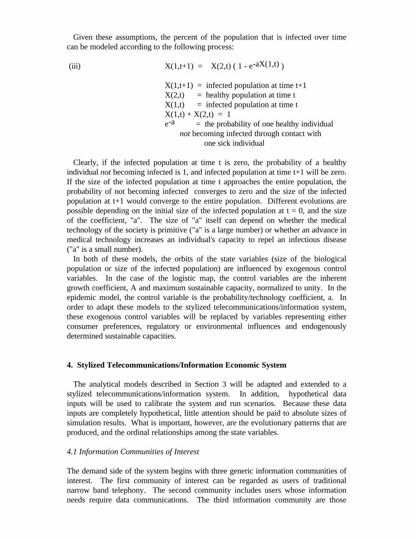
Given these assumptions, the percent of the population that is infected over timecan be modeled according to the following process:
(iii) X(1,t+1) = X(2,t) ( 1 - e-aX(1,t) )
X(1,t+1) = infected population at time t+1X(2,t) = healthy population at time tX(1,t) = infected population at time tX(1,t) + X(2,t) = 1e-a = the probability of one healthy individual not becoming infected through contact with
one sick individual
Clearly, if the infected population at time t is zero, the probability of a healthyindividual not becoming infected is 1, and infected population at time t+1 will be zero.If the size of the infected population at time t approaches the entire population, theprobability of not becoming infected converges to zero and the size of the infectedpopulation at t+1 would converge to the entire population. Different evolutions arepossible depending on the initial size of the infected population at t = 0, and the sizeof the coefficient, "a". The size of "a" itself can depend on whether the medicaltechnology of the society is primitive ("a" is a large number) or whether an advance inmedical technology increases an individual's capacity to repel an infectious disease("a" is a small number). In both of these models, the orbits of the state variables (size of the biologicalpopulation or size of the infected population) are influenced by exogenous controlvariables. In the case of the logistic map, the control variables are the inherentgrowth coefficient, A and maximum sustainable capacity, normalized to unity. In theepidemic model, the control variable is the probability/technology coefficient, a. Inorder to adapt these models to the stylized telecommunications/information system,these exogenous control variables will be replaced by variables representing eitherconsumer preferences, regulatory or environmental influences and endogenouslydetermined sustainable capacities.
4. Stylized Telecommunications/Information Economic System
The analytical models described in Section 3 will be adapted and extended to astylized telecommunications/information system. In addition, hypothetical datainputs will be used to calibrate the system and run scenarios. Because these datainputs are completely hypothetical, little attention should be paid to absolute sizes ofsimulation results. What is important, however, are the evolutionary patterns that areproduced, and the ordinal relationships among the state variables.
4.1 Information Communities of Interest
The demand side of the system begins with three generic information communities ofinterest. The first community of interest can be regarded as users of traditionalnarrow band telephony. The second community includes users whose informationneeds require data communications. The third information community are those
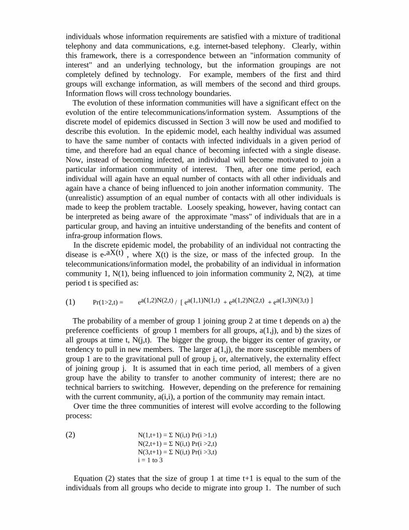
individuals whose information requirements are satisfied with a mixture of traditionaltelephony and data communications, e.g. internet-based telephony. Clearly, withinthis framework, there is a correspondence between an "information community ofinterest" and an underlying technology, but the information groupings are notcompletely defined by technology. For example, members of the first and thirdgroups will exchange information, as will members of the second and third groups.Information flows will cross technology boundaries. The evolution of these information communities will have a significant effect on theevolution of the entire telecommunications/information system. Assumptions of thediscrete model of epidemics discussed in Section 3 will now be used and modified todescribe this evolution. In the epidemic model, each healthy individual was assumedto have the same number of contacts with infected individuals in a given period oftime, and therefore had an equal chance of becoming infected with a single disease.Now, instead of becoming infected, an individual will become motivated to join aparticular information community of interest. Then, after one time period, eachindividual will again have an equal number of contacts with all other individuals andagain have a chance of being influenced to join another information community. The(unrealistic) assumption of an equal number of contacts with all other individuals ismade to keep the problem tractable. Loosely speaking, however, having contact canbe interpreted as being aware of the approximate "mass" of individuals that are in aparticular group, and having an intuitive understanding of the benefits and content ofinfra-group information flows. In the discrete epidemic model, the probability of an individual not contracting thedisease is e-aX(t) , where X(t) is the size, or mass of the infected group. In thetelecommunications/information model, the probability of an individual in informationcommunity 1, N(1), being influenced to join information community 2, N(2), at timeperiod t is specified as:
(1) Pr(1>2,t) = ea(1,2)N(2,t) / [ ea(1,1)N(1,t) + ea(1,2)N(2,t) + ea(1,3)N(3,t) ]
The probability of a member of group 1 joining group 2 at time t depends on a) thepreference coefficients of group 1 members for all groups, a(1,j), and b) the sizes ofall groups at time t, N(j,t). The bigger the group, the bigger its center of gravity, ortendency to pull in new members. The larger a(1,j), the more susceptible members ofgroup 1 are to the gravitational pull of group j, or, alternatively, the externality effectof joining group j. It is assumed that in each time period, all members of a givengroup have the ability to transfer to another community of interest; there are notechnical barriers to switching. However, depending on the preference for remainingwith the current community, a(i,i), a portion of the community may remain intact. Over time the three communities of interest will evolve according to the followingprocess:
(2) N(1,t+1) = Σ N(i,t) Pr(i >1,t)N(2,t+1) = Σ N(i,t) Pr(i >2,t)N(3,t+1) = Σ N(i,t) Pr(i >3,t)i = 1 to 3
Equation (2) states that the size of group 1 at time t+1 is equal to the sum of theindividuals from all groups who decide to migrate into group 1. The number of such
individuals is equal to the sizes of the respective communities in the previous timeperiod multiplied by the proportion of each group inclined towards community 1. The following hypothetical numbers were used to calibrate the model:
Table 1Population Preference Coefficients a(i,j)
for Communities of Interest
InformationCommunity
1 2 3
1 (initial size=74) 0 0.100 0.1202 (initial size=15) 0.100 0.037 0.0353 (initial size=10) 0.120 0.035 0.073
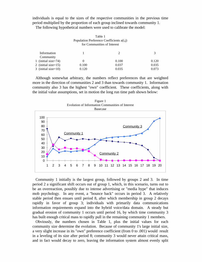
Although somewhat arbitrary, the numbers reflect preferences that are weightedmore in the direction of communities 2 and 3 than towards community 1. Informationcommunity also 3 has the highest "own" coefficient. These coefficients, along withthe initial value assumptions, set in motion the long run time path shown below:
Figure 1Evolution of Information Communities of Interest
Basecase
0102030405060708090
100
1 2 3 4 5 6 7 8 9 10 11 12 13 14 15 16 17 18 19 20
Community 1
Community 2
Community 3
Community 1 initially is the largest group, followed by groups 2 and 3. In timeperiod 2 a significant shift occurs out of group 1, which, in this scenario, turns out tobe an overreaction, possibly due to intense advertising or "media hype" that inducesmob psychology. In any event, a "bounce back" occurs in period 3. A relativelystable period then ensues until period 8, after which membership in group 2 decaysrapidly in favor of group 3; individuals with primarily data communicationsinformation requirements expand into the hybrid voice/data domain. A steady butgradual erosion of community 1 occurs until period 16, by which time community 3has built enough critical mass to rapidly pull in the remaining community 1 members. Obviously, the numbers chosen in Table 1, plus the initial values for eachcommunity size determine the evolution. Because of community 1's large initial size,a very slight increase in its "own" preference coefficient (from 0 to .001) would resultin a leveling of its size after period 8; community 3 would never attain critical mass,and in fact would decay to zero, leaving the information system almost evenly split
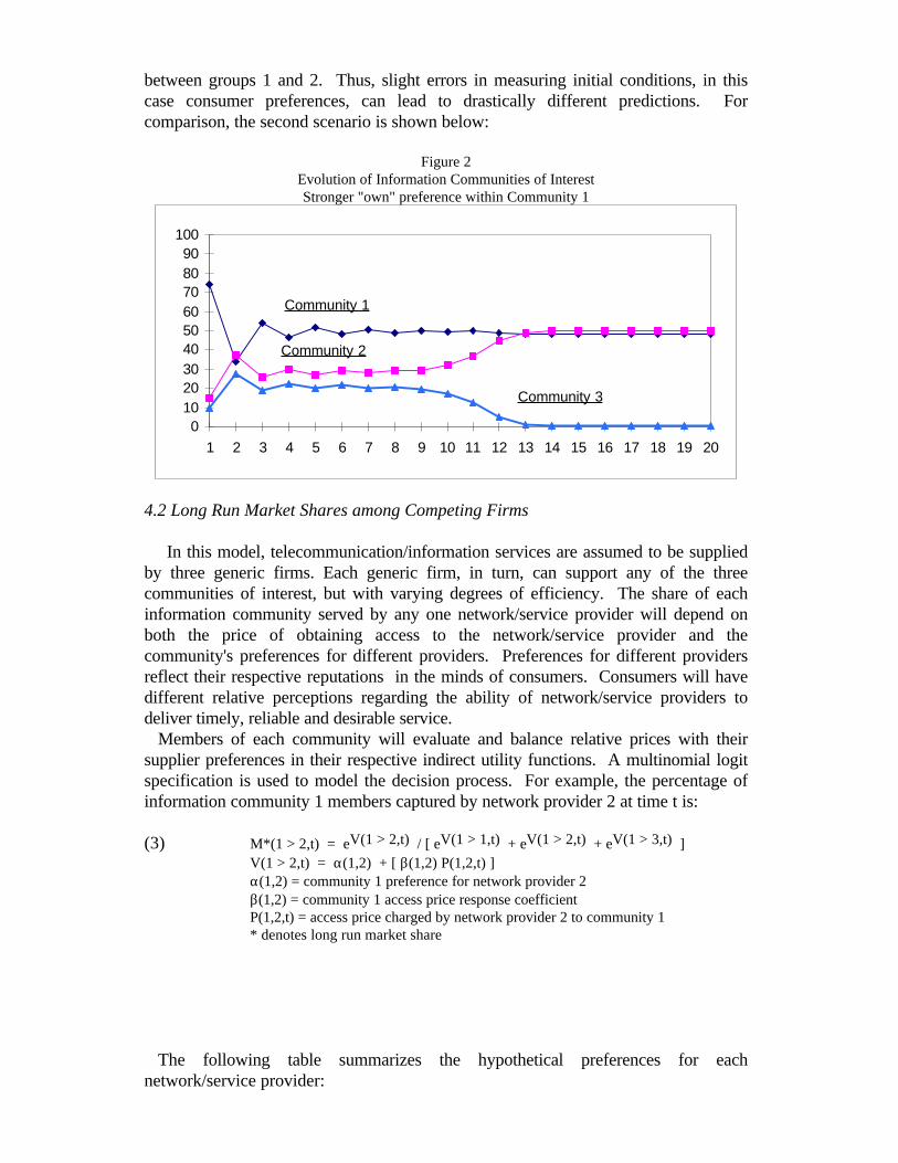
between groups 1 and 2. Thus, slight errors in measuring initial conditions, in thiscase consumer preferences, can lead to drastically different predictions. Forcomparison, the second scenario is shown below:
Figure 2Evolution of Information Communities of InterestStronger "own" preference within Community 1
0102030405060708090
100
1 2 3 4 5 6 7 8 9 10 11 12 13 14 15 16 17 18 19 20
Community 1
Community 2
Community 3
4.2 Long Run Market Shares among Competing Firms
In this model, telecommunication/information services are assumed to be suppliedby three generic firms. Each generic firm, in turn, can support any of the threecommunities of interest, but with varying degrees of efficiency. The share of eachinformation community served by any one network/service provider will depend onboth the price of obtaining access to the network/service provider and thecommunity's preferences for different providers. Preferences for different providersreflect their respective reputations in the minds of consumers. Consumers will havedifferent relative perceptions regarding the ability of network/service providers todeliver timely, reliable and desirable service. Members of each community will evaluate and balance relative prices with theirsupplier preferences in their respective indirect utility functions. A multinomial logitspecification is used to model the decision process. For example, the percentage ofinformation community 1 members captured by network provider 2 at time t is:
(3) M*(1 > 2,t) = eV(1 > 2,t) / [ eV(1 > 1,t) + eV(1 > 2,t) + eV(1 > 3,t) ]V(1 > 2,t) = α(1,2) + [ β(1,2) P(1,2,t) ]α(1,2) = community 1 preference for network provider 2β(1,2) = community 1 access price response coefficientP(1,2,t) = access price charged by network provider 2 to community 1* denotes long run market share
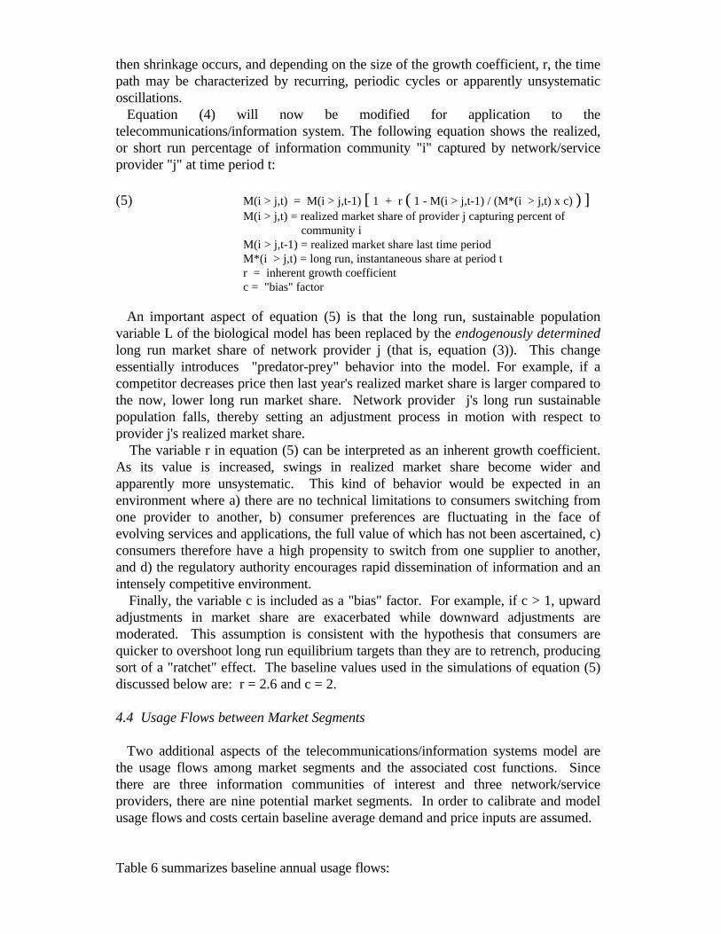
The following table summarizes the hypothetical preferences for eachnetwork/service provider:
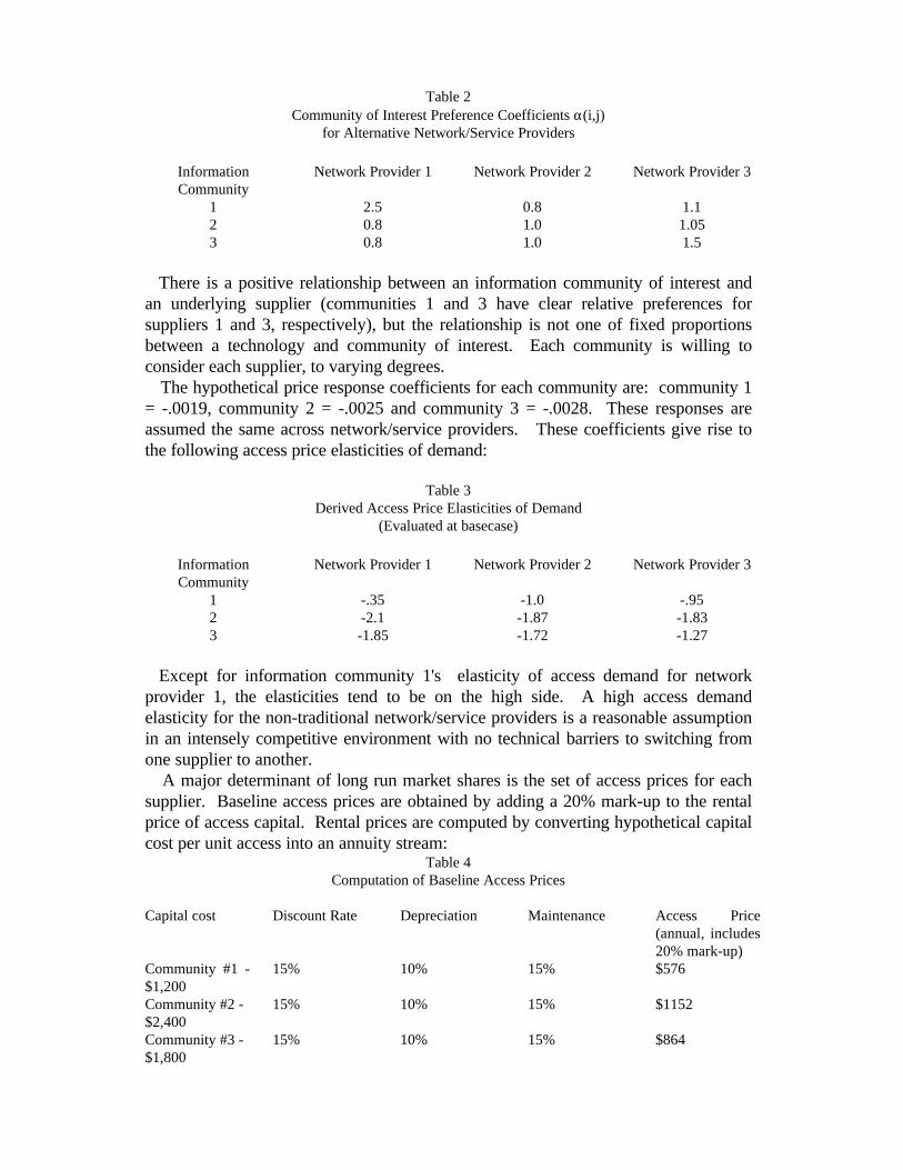
Table 2Community of Interest Preference Coefficients α(i,j)
for Alternative Network/Service Providers
InformationCommunity
Network Provider 1 Network Provider 2 Network Provider 3
1 2.5 0.8 1.12 0.8 1.0 1.053 0.8 1.0 1.5
There is a positive relationship between an information community of interest andan underlying supplier (communities 1 and 3 have clear relative preferences forsuppliers 1 and 3, respectively), but the relationship is not one of fixed proportionsbetween a technology and community of interest. Each community is willing toconsider each supplier, to varying degrees. The hypothetical price response coefficients for each community are: community 1= -.0019, community 2 = -.0025 and community 3 = -.0028. These responses areassumed the same across network/service providers. These coefficients give rise tothe following access price elasticities of demand:
Table 3Derived Access Price Elasticities of Demand
(Evaluated at basecase)
InformationCommunity
Network Provider 1 Network Provider 2 Network Provider 3
1 -.35 -1.0 -.952 -2.1 -1.87 -1.833 -1.85 -1.72 -1.27
Except for information community 1's elasticity of access demand for networkprovider 1, the elasticities tend to be on the high side. A high access demandelasticity for the non-traditional network/service providers is a reasonable assumptionin an intensely competitive environment with no technical barriers to switching fromone supplier to another. A major determinant of long run market shares is the set of access prices for eachsupplier. Baseline access prices are obtained by adding a 20% mark-up to the rentalprice of access capital. Rental prices are computed by converting hypothetical capitalcost per unit access into an annuity stream:
Table 4Computation of Baseline Access Prices
Capital cost Discount Rate Depreciation Maintenance Access Price(annual, includes20% mark-up)
Community #1 -$1,200
15% 10% 15% $576
Community #2 -$2,400
15% 10% 15% $1152
Community #3 -$1,800
15% 10% 15% $864

The capital cost figures assume economies of scope in the provision of access forinformation community 3, relative to separate provisioning of service for communities1 and 2. Finally, long run market shares are obtained by inserting the baseline access pricesinto the indirect utility functions described above:
Table 5Derived Long Run Market Shares
(Evaluated at Baseline)
InformationCommunity
Network Provider 1 Network Provider 2 Network Provider 3
1 70% 12.8% 17.3%2 28.5% 34.8% 36.6%3 23.6% 28.8% 47.5%
4.3 Short Run Market Shares among Competing Firms
The market shares shown in Table 5 are long run shares. Long run shares will notbe attained instantly. An adjustment period will occur during which new informationthat affects decision making will diffuse through the system. Once the informationreaches consumers it may take an additional amount of time for consumers to react tothe new data. If the initial reaction is too strong, consumers may retrench, and thisprocess may repeat itself a number of times. The initial reaction might be too strongif consumers are made to feel that they must choose quickly, or risk being left behindthe "new information age". Traditional types of adjustment mechanisms used ineconomics usually give rise to a) trajectories that reach the long run steady stateasymptotically (Koyck lag), or b) inverted "U"-shaped response curves that aresmooth and continuous (Polynomial Distributed Lag). [ ] The experience in the longdistance market, however, suggests that long run equilibrium market shares may becharacterized by a permanent amount of churn as consumers move from one providerto the other. In the long distance market this activity has been primarily driven byprice. Going forward, however, the telecommunications/information system will betransformed in unprecedented ways; existing firms and new entrants will carry bothtraditional and new services and applications. The nature of these services andapplications will be modified and consumer's preferences will adapt and adjust tochanging regimes. In this context, it is reasonable to assume that as consumers striveto reach a long run equilibrium target that itself is evolving, the observed transitionpath towards long run market shares will be anything but smooth and asymptotic. One variation of the logistic map discussed in Section 3 that has been used inmodeling biological populations is:
(4) dP/dt = rP[ 1 - (P/L) ]dP/dt = rate of change in population at time tP = population level at time tr = inherent growth coefficientL = maximum sustainable population
In this formulation, the population grows as long as it remains below its maximumsustainable level, L. Maximum sustainable level would be determined by food supply,for example, or the existence of a predator population If actual population exceeds L,
then shrinkage occurs, and depending on the size of the growth coefficient, r, the timepath may be characterized by recurring, periodic cycles or apparently unsystematicoscillations. Equation (4) will now be modified for application to thetelecommunications/information system. The following equation shows the realized,or short run percentage of information community "i" captured by network/serviceprovider "j" at time period t:
(5) M(i > j,t) = M(i > j,t-1) [ 1 + r ( 1 - M(i > j,t-1) / (M*(i > j,t) x c) ) ]M(i > j,t) = realized market share of provider j capturing percent of
community iM(i > j,t-1) = realized market share last time periodM*(i > j,t) = long run, instantaneous share at period tr = inherent growth coefficientc = "bias" factor
An important aspect of equation (5) is that the long run, sustainable populationvariable L of the biological model has been replaced by the endogenously determinedlong run market share of network provider j (that is, equation (3)). This changeessentially introduces "predator-prey" behavior into the model. For example, if acompetitor decreases price then last year's realized market share is larger compared tothe now, lower long run market share. Network provider j's long run sustainablepopulation falls, thereby setting an adjustment process in motion with respect toprovider j's realized market share. The variable r in equation (5) can be interpreted as an inherent growth coefficient.As its value is increased, swings in realized market share become wider andapparently more unsystematic. This kind of behavior would be expected in anenvironment where a) there are no technical limitations to consumers switching fromone provider to another, b) consumer preferences are fluctuating in the face ofevolving services and applications, the full value of which has not been ascertained, c)consumers therefore have a high propensity to switch from one supplier to another,and d) the regulatory authority encourages rapid dissemination of information and anintensely competitive environment. Finally, the variable c is included as a "bias" factor. For example, if c > 1, upwardadjustments in market share are exacerbated while downward adjustments aremoderated. This assumption is consistent with the hypothesis that consumers arequicker to overshoot long run equilibrium targets than they are to retrench, producingsort of a "ratchet" effect. The baseline values used in the simulations of equation (5)discussed below are: r = 2.6 and c = 2.
4.4 Usage Flows between Market Segments
Two additional aspects of the telecommunications/information systems model arethe usage flows among market segments and the associated cost functions. Sincethere are three information communities of interest and three network/serviceproviders, there are nine potential market segments. In order to calibrate and modelusage flows and costs certain baseline average demand and price inputs are assumed.
Table 6 summarizes baseline annual usage flows:

Table 6Baseline Average Annual Usage Flows
(Market segments = a,b,c,d,e,f,g,h,i)Usage flows
usage originating from segment X to Y at unit priceOriginating segment = average flow per unit in terminating segment
segments Information community # 1 a b c d e f g h ia Network provider # 1 100 100 100 0 0 0 60 60 60b Network provider # 2 100 100 100 0 0 0 60 60 60c Network provider # 3 100 100 100 0 0 0 60 60 60
Information community # 2d Network provider # 1 0 0 0 70 70 70 50 50 50e Network provider # 2 0 0 0 70 70 70 50 50 50f Network provider # 3 0 0 0 70 70 70 50 50 50
Information community # 3g Network provider # 1 30 30 30 50 50 50 200 200 200h Network provider # 2 30 30 30 50 50 50 200 200 200i Network provider # 3 30 30 30 50 50 50 200 200 200
Members of each information community are assumed to originate usage tomembers of their own community, regardless of which network/service provider thereceiving members utilize. Members of community 1 and 2, however, do notcommunicate directly, whereas both of these groups do communicate with membersof community 3. The figures in Table 6 represent average usage transmitted perindividual in one market segment to each individual in the terminating marketsegment. Therefore, the total amount of usage originating in segment "a" andterminating in segment "b", for example, is equal to the product of the number ofindividuals in each segment, multiplied by the appropriate usage amount in Table 6. Associated with the baseline average usage flows is a set of assumed priceelasticities of demand:
Table 7Baseline Price Elasticity of Demand(Market segments = a,b,c,d,e,f,g,h,i)
Originating segment = Elasticity assumptions at initial, unit pricesegments Information community # 1 a b c d e f g h i
a Network provider # 1 -0.20 -0.20 -0.20 -0.50 -0.50 -0.50 -0.80 -0.80 -0.80b Network provider # 2 -0.20 -0.20 -0.20 -0.50 -0.50 -0.50 -0.80 -0.80 -0.80c Network provider # 3 -0.20 -0.20 -0.20 -0.50 -0.50 -0.50 -0.80 -0.80 -0.80
Information community # 2d Network provider # 1 -0.50 -0.50 -0.50 -0.20 -0.20 -0.20 -0.80 -0.80 -0.80e Network provider # 2 -0.50 -0.50 -0.50 -0.20 -0.20 -0.20 -0.80 -0.80 -0.80f Network provider # 3 -0.50 -0.50 -0.50 -0.20 -0.20 -0.20 -0.80 -0.80 -0.80
Information community # 3g Network provider # 1 -0.80 -0.80 -0.80 -0.80 -0.80 -0.80 -0.20 -0.20 -0.20h Network provider # 2 -0.80 -0.80 -0.80 -0.80 -0.80 -0.80 -0.20 -0.20 -0.20i Network provider # 3 -0.80 -0.80 -0.80 -0.80 -0.80 -0.80 -0.20 -0.20 -0.20
All of the initial elasticities are set less than unity. The elasticities tend to be largeron usage flows between communities 1 and 3 and between communities 2 and 3.Infra-community price elasticities have the lowest values.
Finally, a set of baseline usage prices is assumed:
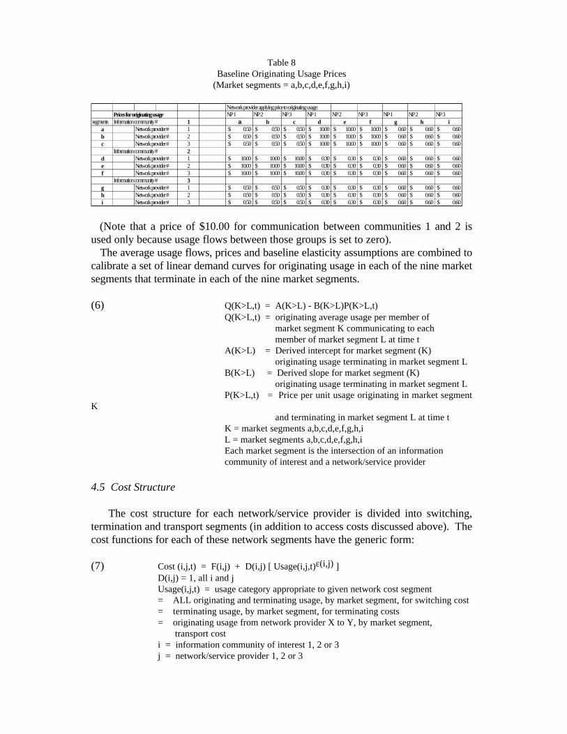
Table 8Baseline Originating Usage Prices
(Market segments = a,b,c,d,e,f,g,h,i)
Network provider applying price to originating usage:Prices for originating usage NP 1 NP 2 NP 3 NP 1 NP 2 NP 3 NP 1 NP 2 NP 3
segments Information community # 1 a b c d e f g h ia Network provider # 1 0.50$ 0.50$ 0.50$ 10.00$ 10.00$ 10.00$ 0.60$ 0.60$ 0.60$ b Network provider # 2 0.50$ 0.50$ 0.50$ 10.00$ 10.00$ 10.00$ 0.60$ 0.60$ 0.60$ c Network provider # 3 0.50$ 0.50$ 0.50$ 10.00$ 10.00$ 10.00$ 0.60$ 0.60$ 0.60$
Information community # 2d Network provider # 1 10.00$ 10.00$ 10.00$ 0.30$ 0.30$ 0.30$ 0.60$ 0.60$ 0.60$ e Network provider # 2 10.00$ 10.00$ 10.00$ 0.30$ 0.30$ 0.30$ 0.60$ 0.60$ 0.60$ f Network provider # 3 10.00$ 10.00$ 10.00$ 0.30$ 0.30$ 0.30$ 0.60$ 0.60$ 0.60$
Information community # 3g Network provider # 1 0.50$ 0.50$ 0.50$ 0.30$ 0.30$ 0.30$ 0.60$ 0.60$ 0.60$ h Network provider # 2 0.50$ 0.50$ 0.50$ 0.30$ 0.30$ 0.30$ 0.60$ 0.60$ 0.60$ i Network provider # 3 0.50$ 0.50$ 0.50$ 0.30$ 0.30$ 0.30$ 0.60$ 0.60$ 0.60$
(Note that a price of $10.00 for communication between communities 1 and 2 isused only because usage flows between those groups is set to zero). The average usage flows, prices and baseline elasticity assumptions are combined tocalibrate a set of linear demand curves for originating usage in each of the nine marketsegments that terminate in each of the nine market segments.
(6) Q(K>L,t) = A(K>L) - B(K>L)P(K>L,t)Q(K>L,t) = originating average usage per member of
market segment K communicating to each member of market segment L at time t
A(K>L) = Derived intercept for market segment (K) originating usage terminating in market segment L
B(K>L) = Derived slope for market segment (K) originating usage terminating in market segment L
P(K>L,t) = Price per unit usage originating in market segmentK
and terminating in market segment L at time tK = market segments a,b,c,d,e,f,g,h,iL = market segments a,b,c,d,e,f,g,h,iEach market segment is the intersection of an informationcommunity of interest and a network/service provider
4.5 Cost Structure
The cost structure for each network/service provider is divided into switching,termination and transport segments (in addition to access costs discussed above). Thecost functions for each of these network segments have the generic form:
(7) Cost (i,j,t) = F(i,j) + D(i,j) [ Usage(i,j,t)ε(i,j) ]D(i,j) = 1, all i and jUsage(i,j,t) = usage category appropriate to given network cost segment= ALL originating and terminating usage, by market segment, for switching cost= terminating usage, by market segment, for terminating costs= originating usage from network provider X to Y, by market segment, transport costi = information community of interest 1, 2 or 3j = network/service provider 1, 2 or 3

The functional form, in (7) was chosen because it highlights the significant fixed costcomponent in network cost functions, and it also allows usage-related economies ofscale to be reflected through the term Usage(i,j,t)ε(i,j). If ε(i,j) is 0 there are noeconomies of scale (all costs are fixed). If ε(i,j) is less than 1 there are globaleconomies of scale (average cost per unit usage always declines), and if ε(i,j) exceeds1 average usage cost curves are "U"-shaped. Although all network/service providersare assumed to have the same cost structure as in (7), the magnitudes of thecoefficients differ, reflecting differences in comparative advantage in handlingdifferent types of traffic. These differences are summarized in the following table:
Table 9Cost Function Parameters
Network Network/service Market Intercept ExponentSegment provider segment F(i,j) E(i,j)Switching Network Provider 1 Info community 1 5000 0.950
Info community 2 10000 1.001Info community 3 15000 0.950
Network Provider 2 Info community 1 10000 0.788Info community 2 20000 0.848Info community 3 25000 0.813
Network Provider 3 Info community 1 15800 0.479Info community 2 31200 0.599Info community 3 39502 0.524
Terminating Network Provider 1 Info community 1 1950 0.659Info community 2 3900 0.850Info community 3 5850 0.900
Network Provider 2 Info community 1 4063 0.807Info community 2 8126 0.924Info community 3 6095 0.795
Network Provider 3 Info community 1 6420 0.453Info community 2 12839 0.538Info community 3 9629 0.464
Transport Network Provider 1 Info community 1 5000 0.775(from 1 to 2) Info community 2 10000 0.900
Info community 3 8000 0.950Network Provider1 Info community 1 7000 0.771(from 1 to 3) Info community 2 12000 0.861
Info community 3 10000 0.850Network Provider 2 Info community 1 5000 0.735(from 2 to 1) Info community 2 10000 0.840
Info community 3 8000 0.731Network Provider 2 Info community 1 7000 0.771(from 2 to 3) Info community 2 12000 0.861
Info community 3 10000 0.753Network Provider 3 Info community 1 8295 0.495(from 3 to 1) Info community 2 14220 0.574
Info community 3 11850 0.496Network Provider 3 Info community 1 8295 0.495(from 3 to 2) Info community 2 14220 0.574
Info community 3 11850 0.496
A basic characteristic of these input assumptions is that network provider 3 tends tohave higher fixed cost components than providers 1 and 2, and, in addition, a lower

variable cost component as reflected in its exponent values. Network provider 1tends to be more efficient in handling the usage generated by information community1 than does network provider 2, evaluated at basecase volumes. In general, the fixedcost components associated with information community 3 usage is less than the sumof the fixed components for communities 1 and 2. This characteristic applies to allnetwork providers, reflecting economies of scope in the provision of community 3usage.
4.6 Usage Pricing Rule and Inter-firm payments
The baseline usage pricing rule followed by all providers is assumed to be traditionalprofit maximization, where the previous period marginal cost of usage is used todetermine current period price. The (lagged) marginal cost used by a networkprovider to compute prices for its originating usage consists of switching, transportand terminating marginal cost components. Further, the originating network provideris assumed to reimburse the receiving network provider for all terminating costsassociated with the usage flowing from the former to the latter.
4.7 Regulatory Policy Initiatives
The model allows four types of regulatory policy initiatives to be introduced. First, network provider 1 may be constrained to allocate a portion of its terminationcosts for information community 1 traffic to its termination costs for informationcommunity 2 and community 3 traffic. A regulator might promote this kind ofinitiative to make it easier for new entrants to terminate traditional, community 1 typetraffic into the incumbent's local market. At the same time, this policy would make itmore expensive for newer services applications to terminate in the incumbent's localmarket. A second initiative is the allocation of a portion of provider 1's access costs to itsterminating cost functions for community 2 and community 3 usage. The regulatorymotivation here is to decrease local access prices and the effect, again, is to raise thecost of terminating new forms of information in the incumbent's market. On the otherhand, as competition intensifies for all forms of customers, artificially lowering accessprices gives the incumbent an artificial and inefficient access price advantage. Third, the regulator can delay the incumbent's entry in the provision of new forms oftelecommunications and information services, i.e., community 2 and community 3usage. The motivation of the regulator presumably is to give other firms time to buildcritical mass to sustainable levels, and to prevent the incumbent from using its accessrevenue to cross subside entry into newer markets. The fourth type of policy control considered is forcing the incumbent's usage pricesto either a) equal marginal costs, or to b) maximize revenue instead of profit. Eitherway, price restrictions will force the incumbent into sub-optimal financialperformance. The effects of these regulatory initiatives will be evaluated in terms of operatingnetwork efficiency and realized market shares. Operating network efficiency is definedas the ratio of non-access costs divided by aggregate usage.
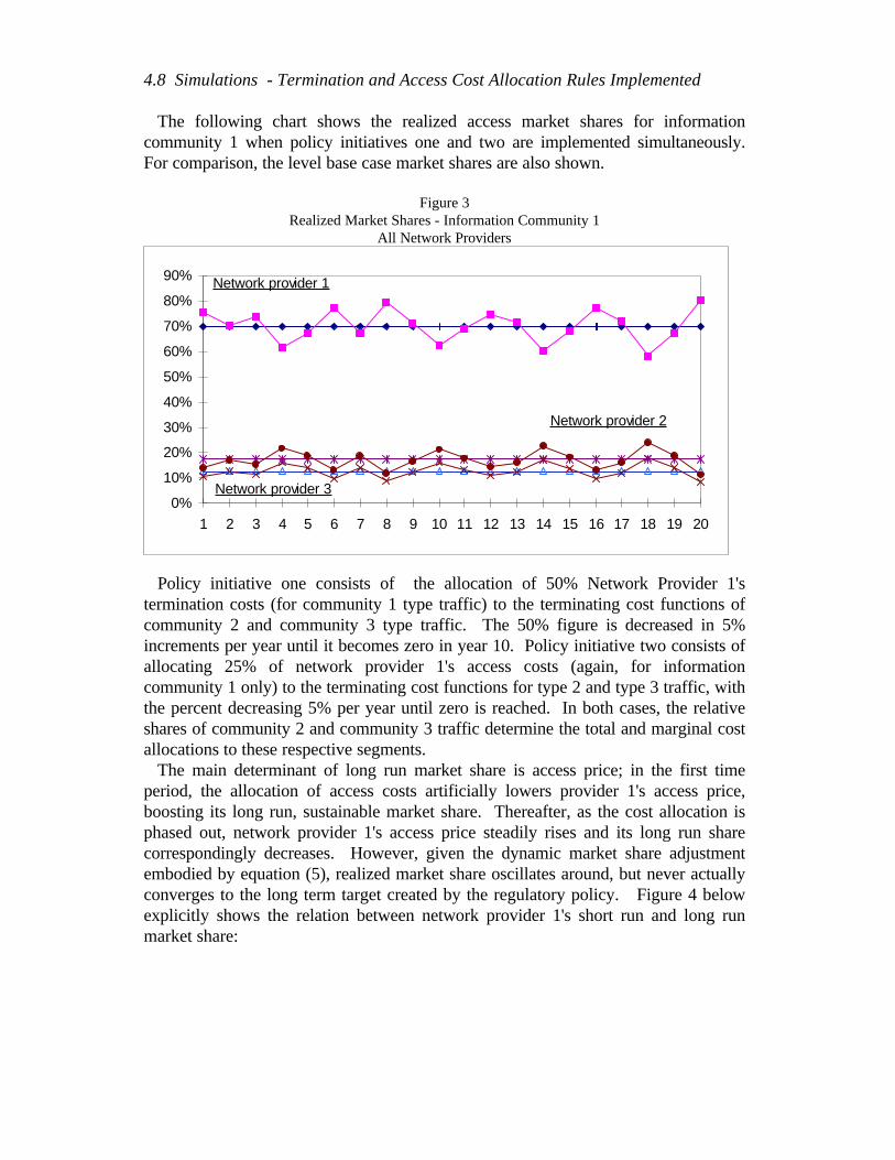
4.8 Simulations - Termination and Access Cost Allocation Rules Implemented
The following chart shows the realized access market shares for informationcommunity 1 when policy initiatives one and two are implemented simultaneously.For comparison, the level base case market shares are also shown.
Figure 3Realized Market Shares - Information Community 1
All Network Providers
0%
10%
20%
30%
40%
50%
60%
70%
80%
90%
1 2 3 4 5 6 7 8 9 10 11 12 13 14 15 16 17 18 19 20
Network provider 2
Network provider 3
Network provider 1
Policy initiative one consists of the allocation of 50% Network Provider 1'stermination costs (for community 1 type traffic) to the terminating cost functions ofcommunity 2 and community 3 type traffic. The 50% figure is decreased in 5%increments per year until it becomes zero in year 10. Policy initiative two consists ofallocating 25% of network provider 1's access costs (again, for informationcommunity 1 only) to the terminating cost functions for type 2 and type 3 traffic, withthe percent decreasing 5% per year until zero is reached. In both cases, the relativeshares of community 2 and community 3 traffic determine the total and marginal costallocations to these respective segments. The main determinant of long run market share is access price; in the first timeperiod, the allocation of access costs artificially lowers provider 1's access price,boosting its long run, sustainable market share. Thereafter, as the cost allocation isphased out, network provider 1's access price steadily rises and its long run sharecorrespondingly decreases. However, given the dynamic market share adjustmentembodied by equation (5), realized market share oscillates around, but never actuallyconverges to the long term target created by the regulatory policy. Figure 4 belowexplicitly shows the relation between network provider 1's short run and long runmarket share:
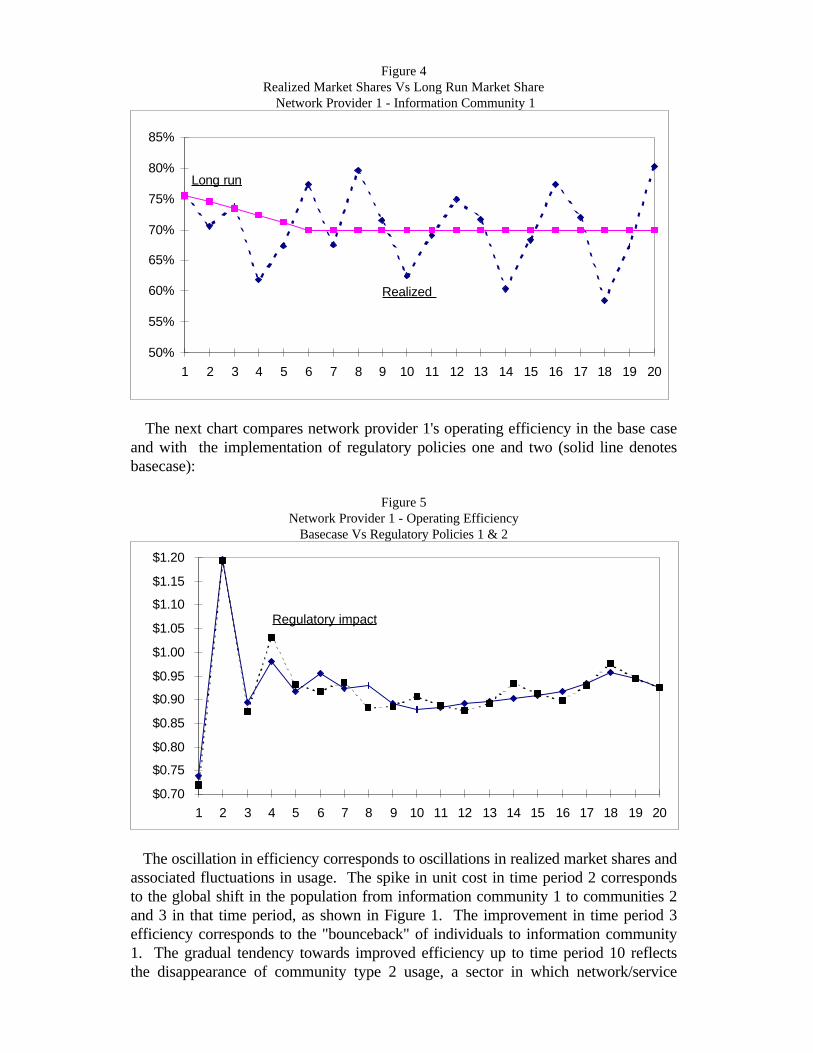
Figure 4Realized Market Shares Vs Long Run Market Share
Network Provider 1 - Information Community 1
50%
55%
60%
65%
70%
75%
80%
85%
1 2 3 4 5 6 7 8 9 10 11 12 13 14 15 16 17 18 19 20
Realized
Long run
The next chart compares network provider 1's operating efficiency in the base caseand with the implementation of regulatory policies one and two (solid line denotesbasecase):
Figure 5Network Provider 1 - Operating Efficiency
Basecase Vs Regulatory Policies 1 & 2
$0.70
$0.75
$0.80
$0.85
$0.90
$0.95
$1.00
$1.05
$1.10
$1.15
$1.20
1 2 3 4 5 6 7 8 9 10 11 12 13 14 15 16 17 18 19 20
Regulatory impact
The oscillation in efficiency corresponds to oscillations in realized market shares andassociated fluctuations in usage. The spike in unit cost in time period 2 correspondsto the global shift in the population from information community 1 to communities 2and 3 in that time period, as shown in Figure 1. The improvement in time period 3efficiency corresponds to the "bounceback" of individuals to information community1. The gradual tendency towards improved efficiency up to time period 10 reflectsthe disappearance of community type 2 usage, a sector in which network/service
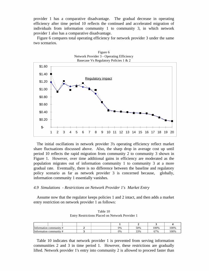
provider 1 has a comparative disadvantage. The gradual decrease in operatingefficiency after time period 10 reflects the continued and accelerated migration ofindividuals from information community 1 to community 3, in which networkprovider 1 also has a comparative disadvantage. Figure 6 compares total operating efficiency for network provider 3 under the sametwo scenarios.
Figure 6Network Provider 3 - Operating Efficiency
Basecase Vs Regulatory Policies 1 & 2
$-
$0.20
$0.40
$0.60
$0.80
$1.00
$1.20
$1.40
$1.60
1 2 3 4 5 6 7 8 9 10 11 12 13 14 15 16 17 18 19 20
Regulatory impact
The initial oscillations in network provider 3's operating efficiency reflect marketshare fluctuations discussed above. Also, the sharp drop in average cost up untilperiod 10 reflects the rapid migration from community 2 to community 3 shown inFigure 1. However, over time additional gains in efficiency are moderated as thepopulation migrates out of information community 1 to community 3 at a moregradual rate. Eventually, there is no difference between the baseline and regulatorypolicy scenario as far as network provider 3 is concerned because, globally,information community 1 essentially vanishes.
4.9 Simulations - Restrictions on Network Provider 1's Market Entry
Assume now that the regulator keeps policies 1 and 2 intact, and then adds a marketentry restriction on network provider 1 as follows:
Table 10Entry Restrictions Placed on Network Provider 1
1 2 3 4Information community # 2 0% 50% 100% 100%Information community # 3 0% 33% 67% 100%
Table 10 indicates that network provider 1 is prevented from serving informationcommunities 2 and 3 in time period 1. However, these restrictions are graduallylifted. Network provider 1's entry into community 2 is allowed to proceed faster than
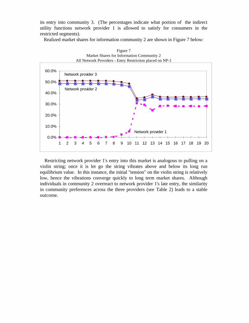
its entry into community 3. (The percentages indicate what portion of the indirectutility functions network provider 1 is allowed to satisfy for consumers in therestricted segments). Realized market shares for information community 2 are shown in Figure 7 below:
Figure 7Market Shares for Information Community 2
All Network Providers - Entry Restriction placed on NP-1
0.0%
10.0%
20.0%
30.0%
40.0%
50.0%
60.0%
1 2 3 4 5 6 7 8 9 10 11 12 13 14 15 16 17 18 19 20
Network provider 3
Network provider 1
Network provider 2
Restricting network provider 1's entry into this market is analogous to pulling on aviolin string; once it is let go the string vibrates above and below its long runequilibrium value. In this instance, the initial "tension" on the violin string is relativelylow, hence the vibrations converge quickly to long term market shares. Althoughindividuals in community 2 overreact to network provider 1's late entry, the similarityin community preferences across the three providers (see Table 2) leads to a stableoutcome.
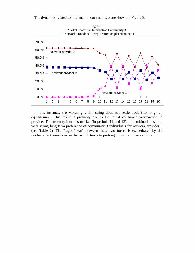
The dynamics related to information community 3 are shown in Figure 8:
Figure 8Market Shares for Information Community 3
All Network Providers - Entry Restriction placed on NP-1
0.0%
10.0%
20.0%
30.0%
40.0%
50.0%
60.0%
70.0%
1 2 3 4 5 6 7 8 9 10 11 12 13 14 15 16 17 18 19 20
Network provider 3
Network provider 2
Network provider 1
In this instance, the vibrating violin string does not settle back into long runequilibrium. This result is probably due to the initial consumer overreaction toprovider 1's late entry into this market (in periods 11 and 12), in combination with avery strong long term preference of community 3 individuals for network provider 3(see Table 2). The "tug of war" between these two forces is exacerbated by theratchet effect mentioned earlier which tends to prolong consumer overreactions.
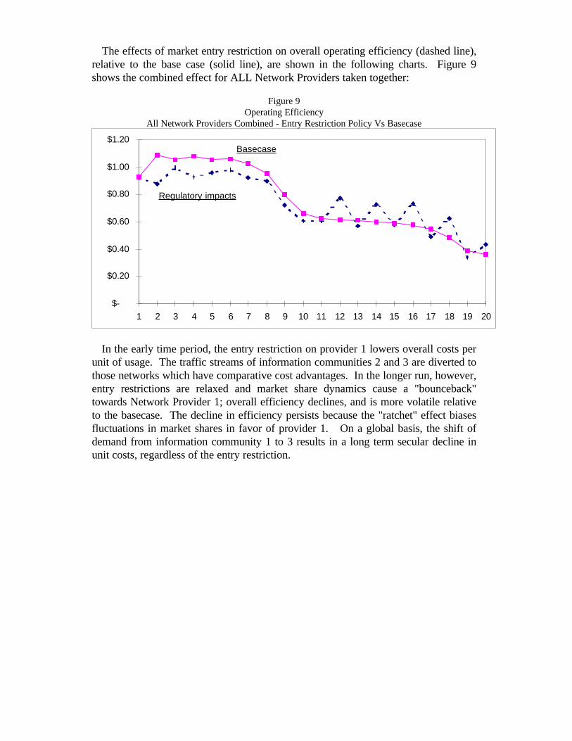
The effects of market entry restriction on overall operating efficiency (dashed line),relative to the base case (solid line), are shown in the following charts. Figure 9shows the combined effect for ALL Network Providers taken together:
Figure 9Operating Efficiency
All Network Providers Combined - Entry Restriction Policy Vs Basecase
$-
$0.20
$0.40
$0.60
$0.80
$1.00
$1.20
1 2 3 4 5 6 7 8 9 10 11 12 13 14 15 16 17 18 19 20
Regulatory impacts
Basecase
In the early time period, the entry restriction on provider 1 lowers overall costs perunit of usage. The traffic streams of information communities 2 and 3 are diverted tothose networks which have comparative cost advantages. In the longer run, however,entry restrictions are relaxed and market share dynamics cause a "bounceback"towards Network Provider 1; overall efficiency declines, and is more volatile relativeto the basecase. The decline in efficiency persists because the "ratchet" effect biasesfluctuations in market shares in favor of provider 1. On a global basis, the shift ofdemand from information community 1 to 3 results in a long term secular decline inunit costs, regardless of the entry restriction.
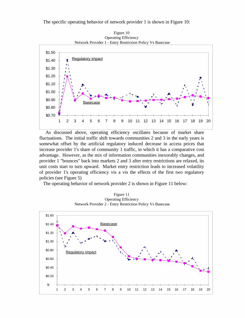
The specific operating behavior of network provider 1 is shown in Figure 10:
Figure 10Operating Efficiency
Network Provider 1 - Entry Restriction Policy Vs Basecase
$0.70
$0.80
$0.90
$1.00
$1.10
$1.20
$1.30
$1.40
$1.50
1 2 3 4 5 6 7 8 9 10 11 12 13 14 15 16 17 18 19 20
Basecase
Regulatory impact
As discussed above, operating efficiency oscillates because of market sharefluctuations. The initial traffic shift towards communities 2 and 3 in the early years issomewhat offset by the artificial regulatory induced decrease in access prices thatincrease provider 1's share of community 1 traffic, in which it has a comparative costadvantage. However, as the mix of information communities inexorably changes, andprovider 1 "bounces" back into markets 2 and 3 after entry restrictions are relaxed, itsunit costs start to turn upward. Market entry restriction leads to increased volatilityof provider 1's operating efficiency vis a vis the effects of the first two regulatorypolicies (see Figure 5) The operating behavior of network provider 2 is shown in Figure 11 below:
Figure 11Operating Efficiency
Network Provider 2 - Entry Restriction Policy Vs Basecase
$-
$0.20
$0.40
$0.60
$0.80
$1.00
$1.20
$1.40
$1.60
1 2 3 4 5 6 7 8 9 10 11 12 13 14 15 16 17 18 19 20
Regulatory impact
Basecase
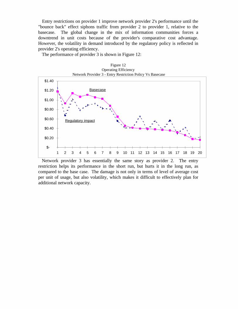
Entry restrictions on provider 1 improve network provider 2's performance until the"bounce back" effect siphons traffic from provider 2 to provider 1, relative to thebasecase. The global change in the mix of information communities forces adowntrend in unit costs because of the provider's comparative cost advantage.However, the volatility in demand introduced by the regulatory policy is reflected inprovider 2's operating efficiency. The performance of provider 3 is shown in Figure 12:
Figure 12Operating Efficiency
Network Provider 3 - Entry Restriction Policy Vs Basecase
$-
$0.20
$0.40
$0.60
$0.80
$1.00
$1.20
$1.40
1 2 3 4 5 6 7 8 9 10 11 12 13 14 15 16 17 18 19 20
Basecase
Regulatory impact
Network provider 3 has essentially the same story as provider 2. The entryrestriction helps its performance in the short run, but hurts it in the long run, ascompared to the base case. The damage is not only in terms of level of average costper unit of usage, but also volatility, which makes it difficult to effectively plan foradditional network capacity.
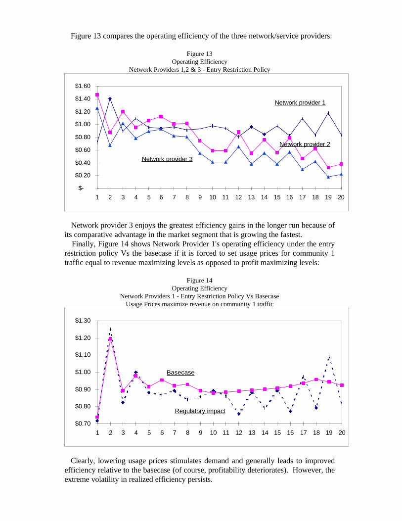
Figure 13 compares the operating efficiency of the three network/service providers:
Figure 13Operating Efficiency
Network Providers 1,2 & 3 - Entry Restriction Policy
$-
$0.20
$0.40
$0.60
$0.80
$1.00
$1.20
$1.40
$1.60
1 2 3 4 5 6 7 8 9 10 11 12 13 14 15 16 17 18 19 20
Network provider 2
Network provider 1
Network provider 3
Network provider 3 enjoys the greatest efficiency gains in the longer run because ofits comparative advantage in the market segment that is growing the fastest. Finally, Figure 14 shows Network Provider 1's operating efficiency under the entryrestriction policy Vs the basecase if it is forced to set usage prices for community 1traffic equal to revenue maximizing levels as opposed to profit maximizing levels:
Figure 14Operating Efficiency
Network Providers 1 - Entry Restriction Policy Vs BasecaseUsage Prices maximize revenue on community 1 traffic
$0.70
$0.80
$0.90
$1.00
$1.10
$1.20
$1.30
1 2 3 4 5 6 7 8 9 10 11 12 13 14 15 16 17 18 19 20
Basecase
Regulatory impact
Clearly, lowering usage prices stimulates demand and generally leads to improvedefficiency relative to the basecase (of course, profitability deteriorates). However, theextreme volatility in realized efficiency persists.
4.10 Simulations - Initial Conditions, Non-Linear Feedback and AlternativeOutcomes to Policy Initiatives
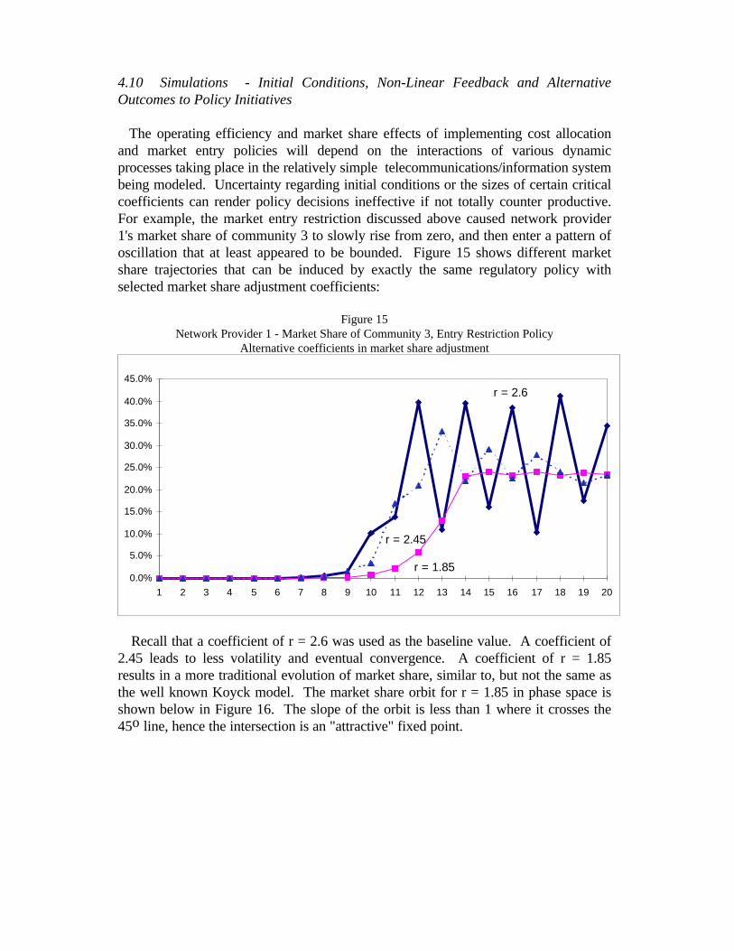
The operating efficiency and market share effects of implementing cost allocationand market entry policies will depend on the interactions of various dynamicprocesses taking place in the relatively simple telecommunications/information systembeing modeled. Uncertainty regarding initial conditions or the sizes of certain criticalcoefficients can render policy decisions ineffective if not totally counter productive.For example, the market entry restriction discussed above caused network provider1's market share of community 3 to slowly rise from zero, and then enter a pattern ofoscillation that at least appeared to be bounded. Figure 15 shows different marketshare trajectories that can be induced by exactly the same regulatory policy withselected market share adjustment coefficients:
Figure 15Network Provider 1 - Market Share of Community 3, Entry Restriction Policy
Alternative coefficients in market share adjustment
0.0%
5.0%
10.0%
15.0%
20.0%
25.0%
30.0%
35.0%
40.0%
45.0%
1 2 3 4 5 6 7 8 9 10 11 12 13 14 15 16 17 18 19 20
r = 2.45
r = 1.85
r = 2.6
Recall that a coefficient of r = 2.6 was used as the baseline value. A coefficient of2.45 leads to less volatility and eventual convergence. A coefficient of r = 1.85results in a more traditional evolution of market share, similar to, but not the same asthe well known Koyck model. The market share orbit for r = 1.85 in phase space isshown below in Figure 16. The slope of the orbit is less than 1 where it crosses the45o line, hence the intersection is an "attractive" fixed point.
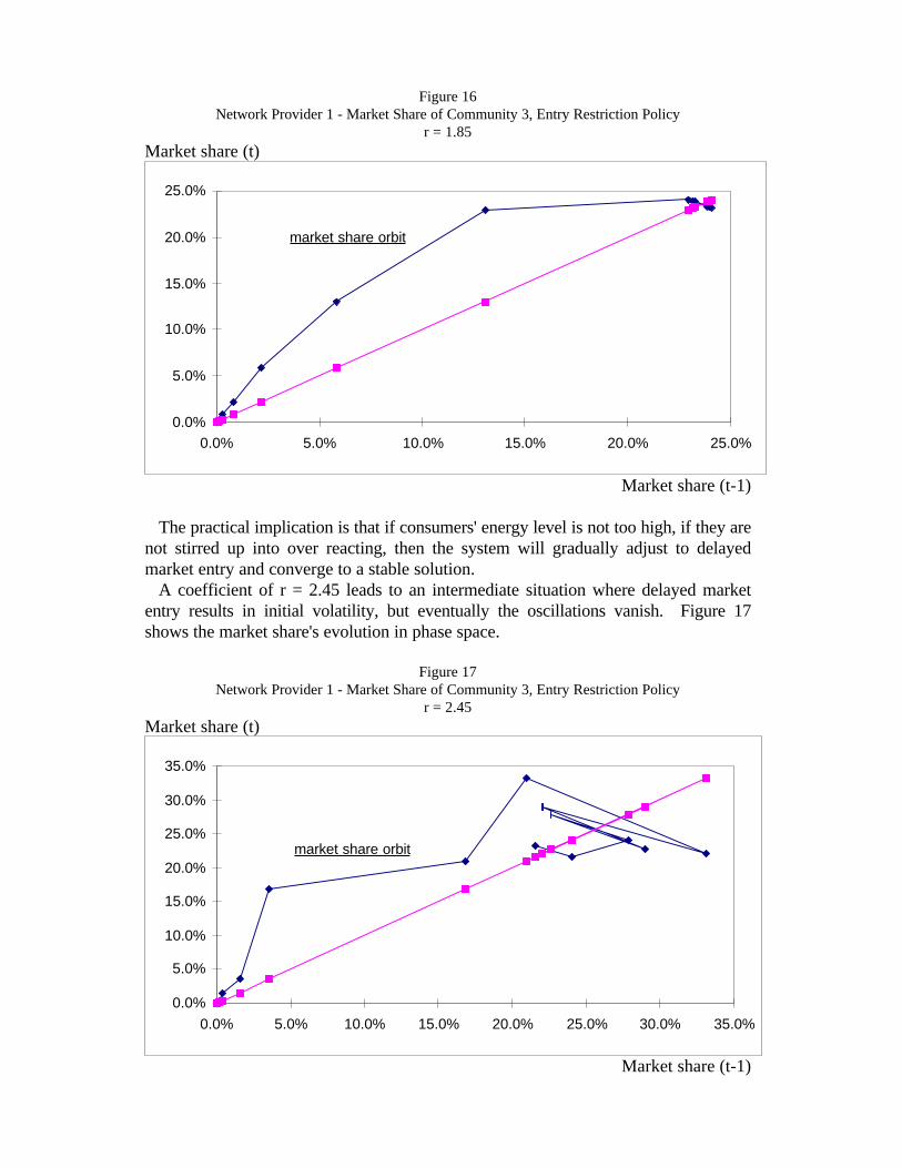
Figure 16Network Provider 1 - Market Share of Community 3, Entry Restriction Policy
r = 1.85Market share (t)
0.0%
5.0%
10.0%
15.0%
20.0%
25.0%
0.0% 5.0% 10.0% 15.0% 20.0% 25.0%
market share orbit
Market share (t-1)
The practical implication is that if consumers' energy level is not too high, if they arenot stirred up into over reacting, then the system will gradually adjust to delayedmarket entry and converge to a stable solution. A coefficient of r = 2.45 leads to an intermediate situation where delayed marketentry results in initial volatility, but eventually the oscillations vanish. Figure 17shows the market share's evolution in phase space.
Figure 17Network Provider 1 - Market Share of Community 3, Entry Restriction Policy
r = 2.45Market share (t)
0.0%
5.0%
10.0%
15.0%
20.0%
25.0%
30.0%
35.0%
0.0% 5.0% 10.0% 15.0% 20.0% 25.0% 30.0% 35.0%
market share orbit
Market share (t-1)
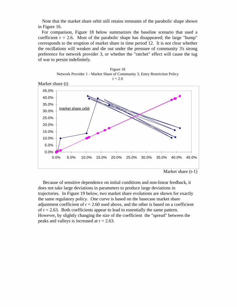
Note that the market share orbit still retains remnants of the parabolic shape shownin Figure 16. For comparison, Figure 18 below summarizes the baseline scenario that used acoefficient r = 2.6. Most of the parabolic shape has disappeared; the large "hump"corresponds to the eruption of market share in time period 12. It is not clear whetherthe oscillations will weaken and die out under the pressure of community 3's strongpreference for network provider 3, or whether the "ratchet" effect will cause the tugof war to persist indefinitely.
Figure 18Network Provider 1 - Market Share of Community 3, Entry Restriction Policy
r = 2.6Market share (t)
0.0%
5.0%
10.0%
15.0%
20.0%
25.0%
30.0%
35.0%
40.0%
45.0%
0.0% 5.0% 10.0% 15.0% 20.0% 25.0% 30.0% 35.0% 40.0% 45.0%
market share orbit
Market share (t-1)
Because of sensitive dependence on initial conditions and non-linear feedback, itdoes not take large deviations in parameters to produce large deviations intrajectories. In Figure 19 below, two market share evolutions are shown for exactlythe same regulatory policy. One curve is based on the basecase market shareadjustment coefficient of r = 2.60 used above, and the other is based on a coefficientof r = 2.63. Both coefficients appear to lead to essentially the same pattern.However, by slightly changing the size of the coefficient the "spread" between thepeaks and valleys is increased at r = 2.63.
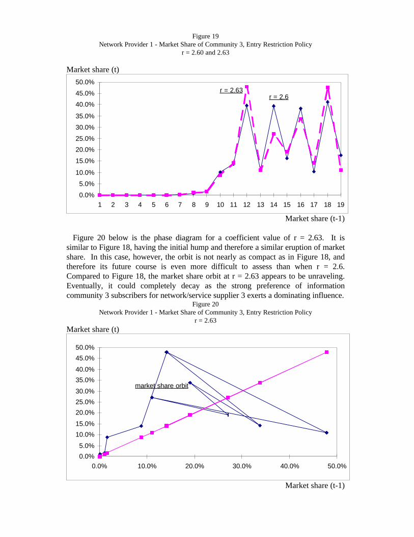
Figure 19Network Provider 1 - Market Share of Community 3, Entry Restriction Policy
r = 2.60 and 2.63
Market share (t)
0.0%
5.0%
10.0%
15.0%
20.0%
25.0%
30.0%
35.0%
40.0%
45.0%
50.0%
1 2 3 4 5 6 7 8 9 10 11 12 13 14 15 16 17 18 19
r = 2.6r = 2.63
Market share (t-1)
Figure 20 below is the phase diagram for a coefficient value of r = 2.63. It issimilar to Figure 18, having the initial hump and therefore a similar eruption of marketshare. In this case, however, the orbit is not nearly as compact as in Figure 18, andtherefore its future course is even more difficult to assess than when r = 2.6.Compared to Figure 18, the market share orbit at r = 2.63 appears to be unraveling.Eventually, it could completely decay as the strong preference of informationcommunity 3 subscribers for network/service supplier 3 exerts a dominating influence.
Figure 20Network Provider 1 - Market Share of Community 3, Entry Restriction Policy
r = 2.63Market share (t)
0.0%
5.0%
10.0%
15.0%
20.0%
25.0%
30.0%
35.0%
40.0%
45.0%
50.0%
0.0% 10.0% 20.0% 30.0% 40.0% 50.0%
market share orbit
Market share (t-1)
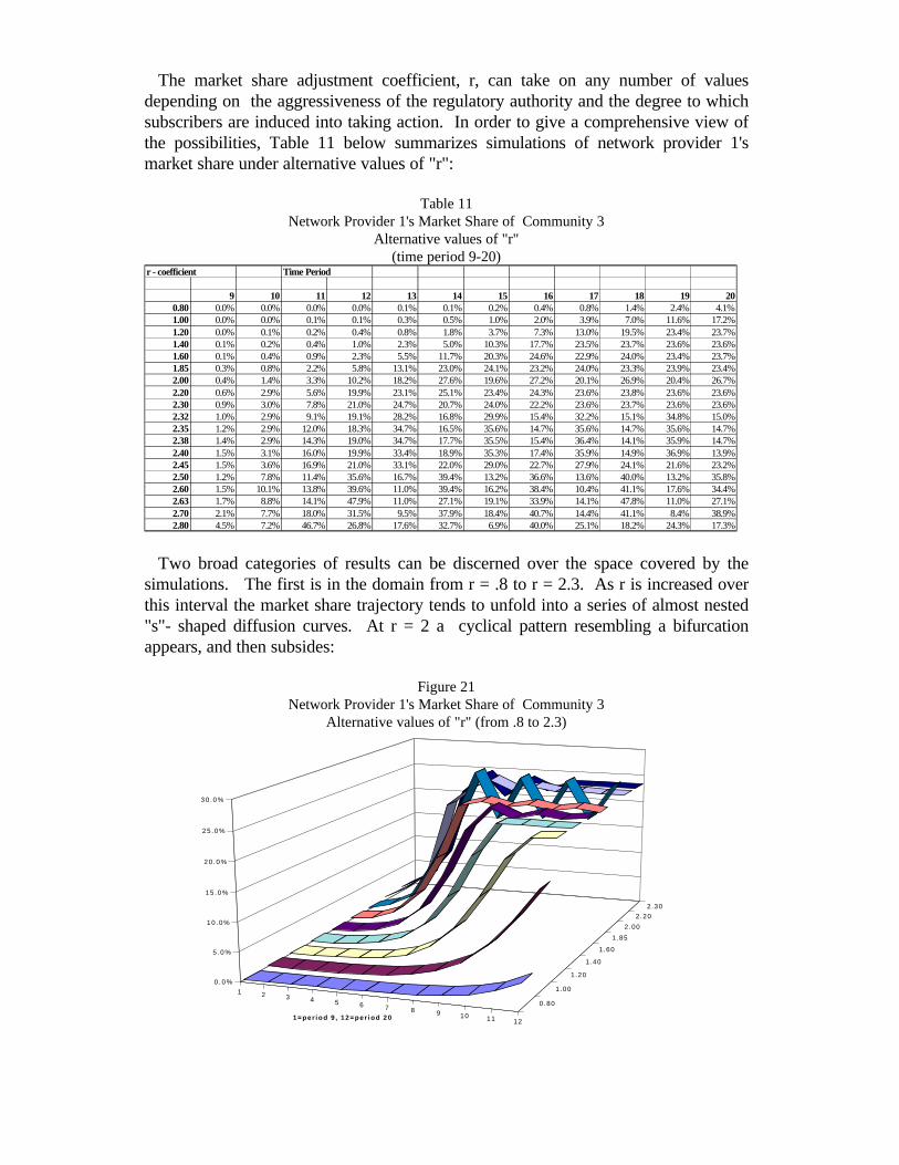
The market share adjustment coefficient, r, can take on any number of valuesdepending on the aggressiveness of the regulatory authority and the degree to whichsubscribers are induced into taking action. In order to give a comprehensive view ofthe possibilities, Table 11 below summarizes simulations of network provider 1'smarket share under alternative values of "r":
Table 11Network Provider 1's Market Share of Community 3
Alternative values of "r"(time period 9-20)
r - coefficient Time Period
9 10 11 12 13 14 15 16 17 18 19 200.80 0.0% 0.0% 0.0% 0.0% 0.1% 0.1% 0.2% 0.4% 0.8% 1.4% 2.4% 4.1%1.00 0.0% 0.0% 0.1% 0.1% 0.3% 0.5% 1.0% 2.0% 3.9% 7.0% 11.6% 17.2%1.20 0.0% 0.1% 0.2% 0.4% 0.8% 1.8% 3.7% 7.3% 13.0% 19.5% 23.4% 23.7%1.40 0.1% 0.2% 0.4% 1.0% 2.3% 5.0% 10.3% 17.7% 23.5% 23.7% 23.6% 23.6%1.60 0.1% 0.4% 0.9% 2.3% 5.5% 11.7% 20.3% 24.6% 22.9% 24.0% 23.4% 23.7%1.85 0.3% 0.8% 2.2% 5.8% 13.1% 23.0% 24.1% 23.2% 24.0% 23.3% 23.9% 23.4%2.00 0.4% 1.4% 3.3% 10.2% 18.2% 27.6% 19.6% 27.2% 20.1% 26.9% 20.4% 26.7%2.20 0.6% 2.9% 5.6% 19.9% 23.1% 25.1% 23.4% 24.3% 23.6% 23.8% 23.6% 23.6%2.30 0.9% 3.0% 7.8% 21.0% 24.7% 20.7% 24.0% 22.2% 23.6% 23.7% 23.6% 23.6%2.32 1.0% 2.9% 9.1% 19.1% 28.2% 16.8% 29.9% 15.4% 32.2% 15.1% 34.8% 15.0%2.35 1.2% 2.9% 12.0% 18.3% 34.7% 16.5% 35.6% 14.7% 35.6% 14.7% 35.6% 14.7%2.38 1.4% 2.9% 14.3% 19.0% 34.7% 17.7% 35.5% 15.4% 36.4% 14.1% 35.9% 14.7%2.40 1.5% 3.1% 16.0% 19.9% 33.4% 18.9% 35.3% 17.4% 35.9% 14.9% 36.9% 13.9%2.45 1.5% 3.6% 16.9% 21.0% 33.1% 22.0% 29.0% 22.7% 27.9% 24.1% 21.6% 23.2%2.50 1.2% 7.8% 11.4% 35.6% 16.7% 39.4% 13.2% 36.6% 13.6% 40.0% 13.2% 35.8%2.60 1.5% 10.1% 13.8% 39.6% 11.0% 39.4% 16.2% 38.4% 10.4% 41.1% 17.6% 34.4%2.63 1.7% 8.8% 14.1% 47.9% 11.0% 27.1% 19.1% 33.9% 14.1% 47.8% 11.0% 27.1%2.70 2.1% 7.7% 18.0% 31.5% 9.5% 37.9% 18.4% 40.7% 14.4% 41.1% 8.4% 38.9%2.80 4.5% 7.2% 46.7% 26.8% 17.6% 32.7% 6.9% 40.0% 25.1% 18.2% 24.3% 17.3%
Two broad categories of results can be discerned over the space covered by thesimulations. The first is in the domain from r = .8 to r = 2.3. As r is increased overthis interval the market share trajectory tends to unfold into a series of almost nested"s"- shaped diffusion curves. At r = 2 a cyclical pattern resembling a bifurcationappears, and then subsides:
Figure 21Network Provider 1's Market Share of Community 3
Alternative values of "r" (from .8 to 2.3)
1 2 3 4 5 6 7 8 9 10 11 12
0.80
1.00
1.20
1.40
1.60
1.85
2.00
2.20
2.30
0 . 0 %
5 . 0 %
10 .0%
15 .0%
20 .0%
25 .0%
30 .0%
1=per iod 9 , 12=per iod 20
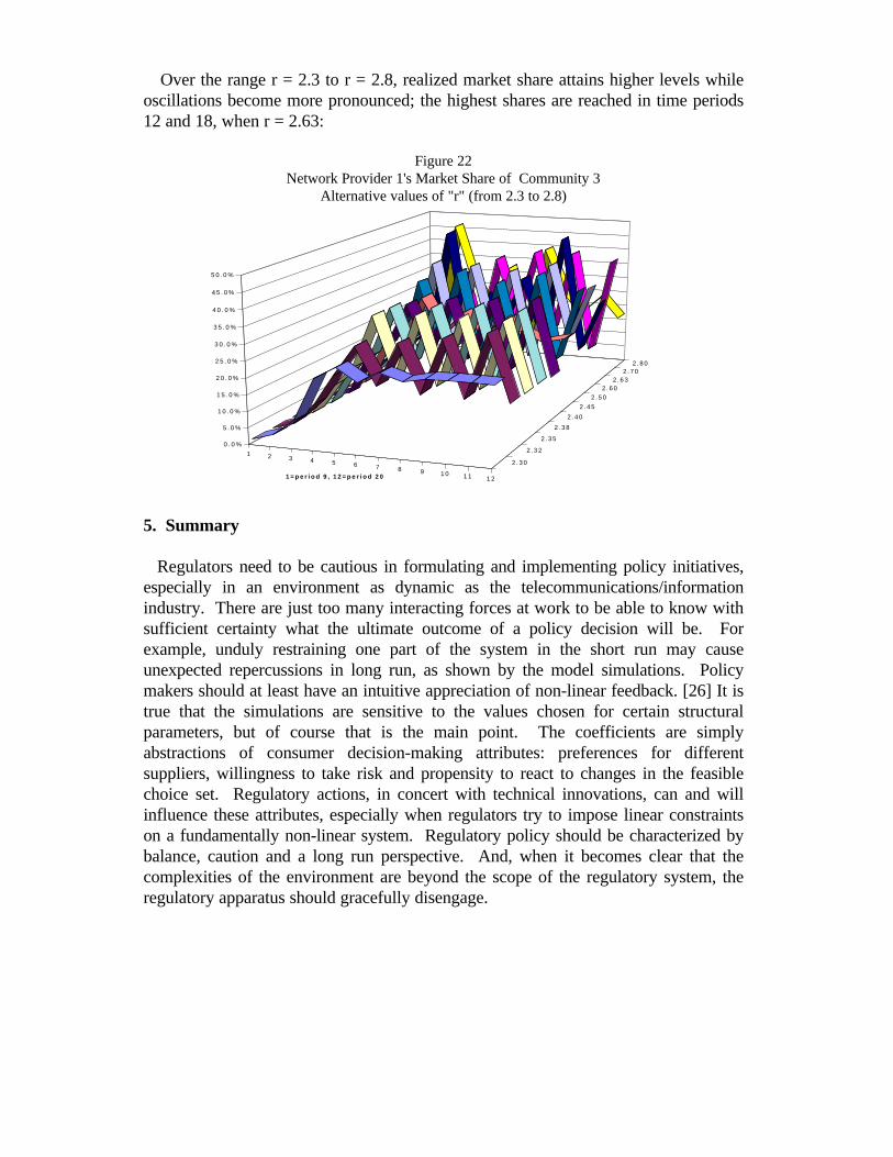
Over the range r = 2.3 to r = 2.8, realized market share attains higher levels whileoscillations become more pronounced; the highest shares are reached in time periods12 and 18, when r = 2.63:
Figure 22Network Provider 1's Market Share of Community 3
Alternative values of "r" (from 2.3 to 2.8)
1 2 3 4 5 6 7 8 9 1 0 1 1 1 2
2 . 3 0
2 . 3 2
2 . 3 5
2 . 3 8
2 . 4 0
2 . 4 5
2 . 5 02 . 6 0
2 . 6 32 . 7 0
2 . 8 0
0 . 0 %
5 . 0 %
1 0 . 0 %
1 5 . 0 %
2 0 . 0 %
2 5 . 0 %
3 0 . 0 %
3 5 . 0 %
4 0 . 0 %
4 5 . 0 %
5 0 . 0 %
1 = p e r i o d 9 , 1 2 = p e r i o d 2 0
5. Summary
Regulators need to be cautious in formulating and implementing policy initiatives,especially in an environment as dynamic as the telecommunications/informationindustry. There are just too many interacting forces at work to be able to know withsufficient certainty what the ultimate outcome of a policy decision will be. Forexample, unduly restraining one part of the system in the short run may causeunexpected repercussions in long run, as shown by the model simulations. Policymakers should at least have an intuitive appreciation of non-linear feedback. [26] It istrue that the simulations are sensitive to the values chosen for certain structuralparameters, but of course that is the main point. The coefficients are simplyabstractions of consumer decision-making attributes: preferences for differentsuppliers, willingness to take risk and propensity to react to changes in the feasiblechoice set. Regulatory actions, in concert with technical innovations, can and willinfluence these attributes, especially when regulators try to impose linear constraintson a fundamentally non-linear system. Regulatory policy should be characterized bybalance, caution and a long run perspective. And, when it becomes clear that thecomplexities of the environment are beyond the scope of the regulatory system, theregulatory apparatus should gracefully disengage.

References
[1] A. Aczel, Fermat's Last Theorem, ISBN: 1 56858 077 0. Four Walls Eight Windows, New York, 1996
[2] M. Asmussen, Regular and Chaotic Cycling in Models from Population and Ecological Genetics. In M. Barnsley and S. Demko (eds). Chaotic Dynamics and Fractals, ISBN: 0 12 079060 2. Academic Press, Inc., New York, 1986
[3] G. Baker and J. Gollub, Chaotic Dynamics, an Introduction, ISBN: 0 521 38897 X. Cambridge University Press, Cambridge, 1990
[4] W. Baumol and E. Wolff, Feedback Between R&D and Productivity Growth: A Chaos Model. In J. Benhabib (ed). Cycles and Chaos in Economic Equilibrium, ISBN: 0 691 00392 0. Princeton University Press, New Jersey, 1992
[5] W. Barnett and P. Chen, An Econometric Application of Mathematical Chaos. In W. Barnett, E. Berndt and H. White (eds). Dynamic Econometric Modeling, ISBN: 0 521 33395 4. Cambridge University Press, Cambridge, 1988
[6] H. Berk, Nonlinear Dynamics of a Driven Mode near Marginal Stability, Physical ReviewLetters Vol 76 Issue 8 (1996) 1256-1259
[7] M. Boldrin and R. Deneckere, Sources of Complex Dynamics in Two-Sector Growth Models. In J. Benhabib (ed). Cycles and Chaos in Economic Equilibrium, ISBN: 0 691 00392 0. Princeton University Press, New Jersey, 1992
[8] M. Boldrin and M. Woodford, Equilibrium Models Displaying Endogenous Fluctuations and Chaos: A Survey. In J. Benhabib (ed). Cycles and Chaos in Economic Equilibrium, ISBN: 0 691 00392 0. Princeton University Press, New Jersey, 1992
[9] P. Drazin, Nonlinear Systems, ISBN: 0 521 40668 4. Cambridge University Press, Cambridge, 1992
[10] A. Einstein, Relativity, The Special and the General Theory, ISBN: 0 517 88441 0. Random House, Inc., New York, 1961
[11] K. Falconer, Fractal Geometry, ISBN: 0 471 92287 0. John Wiley & Sons, New York, 1990
[12] A. Gill, An Equipment Replacement Problem with Dynamic Production Planning and Capacity Considerations, International Journal of Systems Science Vol 27 Issue 10 (1996) 985-988
[13] L. Glass, A. Goldberger, M. Courtemanche and A. Shirer, Nonlinear Dynamics, Chaos and Complex Cardiac Arrhythmias. In M. Berry, I. Percival and N. Weiss (eds). Proceedings of a Royal Society Discussion Meeting, February 4 and 5, 1987, ISBN: 0 521 35455 2. The Royal Society, London, 1987
[14] J Grandmont, Periodic and Aperiodic Behavior in Discrete One-Dimensional Dynamical Systems. In J. Benhabib (ed). Cycles and Chaos in Economic Equilibrium, ISBN: 0 691 003920. Princeton University Press, New Jersey, 1992
[15] H. Haken, Synergetics, ISBN 3 540 08866 0 2. Springer-Verlag, Berlin, 1978
[16] E. Lorenz, The Essence of Chaos, ISBN: 0 295 97514 8. University of Washington Press, Seattle, 1993

[17] R. May, Chaos and the Dynamics of Biological Populations. In M. Berry, I. Percival and N. Weiss (eds). Proceedings of a Royal Society Discussion Meeting, February 4 and 5, 1987, ISBN: 0 521 35455 2. The Royal Society, London, 1987
[18] J. MacQueen, Biological Modeling: Population Dynamics. In C. Bondi (ed). New Applications of Mathematics, Penguin Books, London, 1991
[19] K. Mainzer, Thinking in Complexity, ISBN: 3 540 60637 8. Springer-Verlag, Berlin, 1994
[20] H. Niwa, Mathematical Model for the Size Distribution of Fish Schools, Computers and Mathematics with Applications Vol 32 Issue 11 (1996 ) 79-88
[21] F. Vivaldi, An Experiment in Mathematics. In N. Hall (ed). Exploring Chaos, ISBN: 0 393 31226 7. W. W. Norton, New York, 1991
[22] A. Robson, A Biological Basis for Expected and Non-expected Utility, Journal of Economic Theory Vol 68 Issue 2 (1996) 397-425
[23] D. Ruelle, Diagnosis of Dynamical Systems with Fluctuating Parameters. In M. Berry, I. Percival and N. Weiss (eds). Proceedings of a Royal Society Discussion Meeting, February 4 and 5, 1987, ISBN: 0 521 35455 2. The Royal Society, London, 1987
[24] D. Ruelle, Chance and Chaos, ISBN: 0 691 08574 9. Princeton University Press, 1991
[25] J. Smital, Functions and Functional Equations, ISBN: 0 85274 418 8. IOP Publishing, Ltd., Temple Beck, 1988
[26] N. Stolleman, Some Policy Issues Regarding Interoperability and the National Information Infrastructure, presentation at Interoperability and the Economics of the InformationInfrastructure, Freedom Forum Media Studies Center, sponsored by Science, Technology and Public Policy Program, John F. Kennedy School of Government, Harvard University, 1995
[27] J. Wisdom, Chaotic Behavior in the Solar System. In M. Berry, I. Percival and N. Weiss (eds). Proceedings of a Royal Society Discussion Meeting, February 4 and 5, 1987, ISBN: 0 521 35455 2. The Royal Society, London, 1987
* The views expressed in this paper are those of the author, and do not necessarily reflect the viewsof Telcordia Technologies, nor any of its past, present or future owners and clients.