an analytical framework for the preparation and animation
98
AN ANALYTICAL FRAMEWORK FOR THE PREPARATION AND ANIMATION OF A VIRTUAL MANNEQUIN FOR THE PURPOSE OF MANNEQUIN-CLOTHING INTERACTION MODELING by Matthew Kent Rasmussen A thesis submitted in partial fulfillment of the requirements for the Master of Science degree in Civil and Environmental Engineering in the Graduate College of The University of Iowa December 2008 Thesis Supervisor: Professor Colby C. Swan
-
Upload
khangminh22 -
Category
Documents
-
view
2 -
download
0
Transcript of an analytical framework for the preparation and animation
AN ANALYTICAL FRAMEWORK FOR THE PREPARATION AND ANIMATION
OF A VIRTUAL MANNEQUIN FOR THE PURPOSE OF MANNEQUIN-CLOTHING
INTERACTION MODELING
by
Matthew Kent Rasmussen
A thesis submitted in partial fulfillment of the requirements
for the Master of Science degree in Civil and
Environmental Engineering in the Graduate College of The
University of Iowa
December 2008
Thesis Supervisor: Professor Colby C. Swan

Graduate College
The University of Iowa
Iowa City, Iowa
CERTIFICATE OF APPROVAL
________________________
MASTER’S THESIS
_________________
This is to certify that the Master’s thesis of
Matthew Kent Rasmussen
has been approved by the Examining Committee for the
thesis requirement for the Master of Science degree in Civil
and Environmental Engineering at the December 2008
graduation.
Thesis Committee: _____________________________
Colby C. Swan, Thesis Supervisor
_____________________________
Asghar M. Bhatti
_____________________________
Salam Rahmatalla

ii
To my family and friends for their continued support and encouragement

iii
ACKNOWLEDGEMENTS
Special thanks to Yujiang Xiang for the use and modification of his Denavit-
Hartenberg kinematics software which facilitated conversion of predicted motion joint
angle histories to the control point format used to animate mannequins in this thesis, and
to Timothy Marler and the many others at VSR who were immensely helpful to me in
completing this research.

iv
TABLE OF CONTENTS
LIST OF TABLES........................................................................................................ LIST OF FIGURES...................................................................................................... LIST OF BOXES.......................................................................................................... CHAPTERS
1. INTRODUCTION................................................................................ 1.1 Motivation..................................................................................... 1.2 Objectives and Organization.........................................................
2. LITERATURE REVIEW..................................................................... 3. BODY SCAN PREPARATION...........................................................
3.1 Body Scan Composition................................................................ 3.2 Body Scan Reconstruction............................................................ 3.3 Body Scan Segmentation.............................................................. 3.4 Spherical and Ellipsoidal Joint Segments.....................................
4. VIRTUAL MANNEQUIN ANIMATION...........................................
4.1 Orientating the Mannequin Segments........................................... 4.2 Mannequin Animation with Motion Capture Data....................... 4.3 Mannequin Animation with Joint Angle Histories....................... 4.4 Data Formatting............................................................................
5. CONCLUSION....................................................................................
5.1 Summary....................................................................................... 5.2 Current and Future Work..............................................................
APPENDIX A. 3D DH KINEMATICS NUMERICAL EXAMPLE......................... APPENDIX B. SAMPLE BODY SEGMENT FILE..................................................
APPENDIX C. BODY SEGMENT EDGE CENTROID RESOLVER...................... REFERENCES.............................................................................................................
v
vi
ix
1
12
4
11
11142431
38
38444863
67
6768
72
75
77
86

v
LIST OF TABLES
Tables
A-1 A-2 A-3
A table of link parameters and joint degrees of freedom contributing to the ultimate location of the right wrist at a given point in time........................................................................... The first eight transformation matrix components for each degree of freedom from Table A-1..................................................... The last eight transformation matrix components for each degree of freedom from Table A-1.....................................................
72
73
74

vi
LIST OF FIGURES
Figures
2-1 2-2 2-3 2-4 3-1 3-2 3-3 3-4 3-5 3-6 3-7 3-8 3-9 3-10 3-11 3-12 3-13 3-14 3-15
Human avatar comprised of metaballs................................................ Stick figure animation process............................................................ Ray casting example........................................................................... Mannequin animation snapshots......................................................... The neutral posture with standard axis definition............................... Mesh coarsening comparison.............................................................. The complete right shoulder being used to reconstruct the incomplete scan of the left shoulder................................................... Intersection of sagittal plane with body scan at the incomplete shoulder boundary............................................................................... Formation of the new shoulder boundary........................................... Completed shoulder boundary extrapolation...................................... Mesh reshaping with relocation of existing nodes to coincide with the shoulder boundary nodes...................................................... Shoulder reshaping with addition of new polygons............................ Shoulder reshaping with final set of polygon additions...................... Completed reconstruction of the shoulder.......................................... Graphical explanation of SSI nodes.................................................... Mannequin arm mesh gap................................................................... Reconstructed right arm of the mannequin......................................... Diagram of body segments................................................................. Diagram of body segment edges.........................................................
6
7
8
9
12
14
17
18
18
19
20
21
21
22
23
23
24
25
26

vii
3-16 3-17 3-18 3-19 3-20 3-21 3-22 3-23 4-1 4-2 4-3 4-4 4-5 4-6 4-7 4-8 4-9 5-1 5-2 5-3
Example of an arc-shaped gap............................................................ Front (right) and rear (left) view of the pelvis segment...................... Ray casting automated segmentation result........................................ Circular mesh segment cross-section.................................................. Ellipsoidal mesh segment cross-section.............................................. Frontal view of the pelvis body segment with noted dimensions used for sizing the animation patches................................................. Unpatched (left) and patched (right) animation comparison.............. Diagram of the degrees of freedom used for mannequin animation............................................................................................. Body scan mesh alignment diagram................................................... Hip alignment discrepancy.................................................................. Image of the final mesh alignment step.............................................. Body segment control point diagram.................................................. Mannequin animated with motion capture data.................................. Two-dimensional representation of a kinematic chain....................... A visual definition of DH kinematic parameters and variables in three dimensions................................................................................. An image of SANTOS™ with the DH skeleton overlaid................... Mannequins animated with joint angle data....................................... Perspective view of the mannequin during a clothing interaction simulation............................................................................................ Rear view of the mannequin during a clothing interaction simulation............................................................................................ A second perspective view of the mannequin during a clothing interaction simulation..........................................................................
27
29
31
33
33
34
35
36
40
42
43
45
48
49
55
58
62
69
70
70

viii
5-4
A visual depiction of the closed-loop optimization system for motion prediction................................................................................ 71

ix
LIST OF BOXES
Boxes
4-1
Sample animation control file.............................................................
63
1
CHAPTER 1
INTRODUCTION
1.1 Motivation
The possibility of using computational methods in the research and development
process for textiles and functional clothing has increased with the availability of desktop
computing power. It has been shown experimentally that tight, stiff, bulky clothing can
impede motion or alter strategies for the accomplishment of physical tasks [19]. With
obvious difficulties in measuring clothing resistance forces on a human body undergoing
prescribed motions, the ability to realistically model the mechanics of clothing-body
interactions virtually using computational methods could prove extremely beneficial to
the development of new, less restrictive clothing systems. For example, many of the
current materials used for body armor are known to be very stiff and the resulting
clothing systems restrictive, thus potentially impeding the motion of the wearer. The
ability to realistically model the mechanics of clothing-body interactions is a potentially
significant tool for designing protective clothing systems that are less restrictive.
Any computational framework developed to address the issues noted above will
require a structured procedure involving at least five major steps: (1) the development of
a virtual mannequin, or virtual representation of a human’s body surface; (2) animation of
the virtual mannequin to represent evolution of the body surface during performance of
active tasks; (3) a robust algorithm to detect contact and sliding between the virtual
mannequin and a mathematical clothing model; (4) an algorithm to resolve the contact
forces between the clothing and the mannequin; (5) a realistic model to predict the

2
clothing fabric’s mechanical and dynamic behavior. Significant work has been done
elsewhere for steps (3) through (5) (e.g. [6, 11-13, 19, 21]), and so this thesis will focus
on the first two steps.
1.2 Objectives and Organization
Many works that involve modeling of the human body utilize 3D objects such as
spheres and ellipsoids (e.g. [11-13]), whose bounding surfaces are implicitly defined by a
scalar function of the form ����� = 0, to represent the body. While these make
animation of the body and collision detection simple, they may not accurately represent
the shape of the human body. A more realistic virtual mannequin or avatar will capture
the shape of the individual body parts more accurately, and thus permit truer analysis of
the body-clothing interactions. In this thesis, avatars are developed from 3D laser scans
of human subjects in fixed postures. The resulting body surface meshes are first
decomposed into representative segments in accordance with major sections of the
human body in a process called segmentation, and then manually edited to conform to a
prescribed initial posture. This procedure and its development are presented in Chapter
3.
Next, the rigid body segments are made to translate and rotate in time in
accordance with the performance of active tasks being carried out by a human subject.
Two methods for animating virtual mannequins are presented in this thesis, namely via
joint angle time histories, utilizing the Denavit-Hartenberg (DH) kinematics convention
[2, 25] that has been adopted by the Virtual Soldier Research (VSR) group at The
University of Iowa (the source of the joint angle time histories used in this research) for

3
predicting dynamic motions of skeletal human models [1, 3, 9, 15, 26], and via motion
capture data from a number of key locations on the human subject. The framework
presented in this thesis constructs a dynamic body surface model that moves with the
skeletal human model. This allows for interfacing between clothing modeling and digital
human modeling frameworks. The ability to animate the virtual mannequin with motion
capture data was added because it is presently easier to capture complicated motions
associated with highly dynamic and strenuous physical tasks using motion capture
systems than it is to generate such motions using predictive dynamics algorithms. Both
methods of animation are presented in detail in Chapter 4.
With these major steps complete, a contact model can then be employed to
simulate clothing-mannequin interaction for a prescribed motion and human body scan.
Because the goal of this thesis is strictly to develop a framework for preparing virtual
mannequins for clothing interaction simulations with prescribed motion, no contact
model or clothing behavior model (e.g. finite element or particle methods) is presented in
this work. All clothed mannequin simulations presented use the framework originally
developed by Man, et al. in [11-13] for both contact and clothing behavior modeling, but
are extended for the more realistic avatars developed in this thesis so as to demonstrate
the effective use of the methodologies presented herein.
4
CHAPTER 2
LITERATURE REVIEW
Since the goal of this framework is to develop a standard methodology for
preparing a 3D human body mesh for animation and clothing interaction simulations, no
review of works involving clothing models will be discussed, and the reader is referred
instead to [6] and [11-13]. The clothing behavior and contact algorithm used to model
clothing interaction with the animations developed for this thesis were adopted from [11].
One of the driving factors behind development of body scanners has been the
desire to obtain in an automated fashion more accurate and consistent measurements of
body dimensions for clothing fitting than what tailors and the layman could obtain. As
computer modeling of apparel became more feasible through the availability of faster
computing technology in the 1990s and 2000s, interest in obtaining complete 3D human
body scans also increased. These 3D scans often employ triangulation-based methods to
resolve the surface contours of the subject [22].
Among the works that used body scans to obtain body measurements, Li and
Jones [10] developed an algorithm that was able to take a “lateral slice” (perpendicular to
the direction of the subject’s height) and determine the chest circumference. Their
algorithm first detected the arm outlines before removing the arms and patching the arm
gaps with a curve-fitting function. Pargas, et al. [18] took a similar approach with lateral
slices of the body scan, but their work also proposed methods for determining other
measurements such as arm length and waist circumference.

5
Jones, et al. [7] developed a technique in which a vertical plane of light is
projected by an array of vertically aligned cameras onto a rotating human model through
its axis of rotation. The scattered and reflected light detected by the cameras was used to
compute 3D surface coordinates. Referred to as the Loughborough Anthropometric
Shadow Scanner, this method was advertised as obtaining accuracies of 1.6mm in the
radial direction (as measured from the axis of rotation out to the body surface) and 1mm
vertically.
In 2000, Siebert and Marshall [22] employed light speckle texture projection
photogrammetry, also known as stereo photogrammetry, to obtain human body images.
Originally developed at the Turing Institute, stereo photogrammetry operates by
extrapolating the difference between two images of a surface as seen by adjacent cameras
into a “depth map.” Along with relatively fast data capture, Siebert and Marshall claimed
accuracies of 0.5mm and 2.0mm for the face and body surfaces of the human model,
respectively.
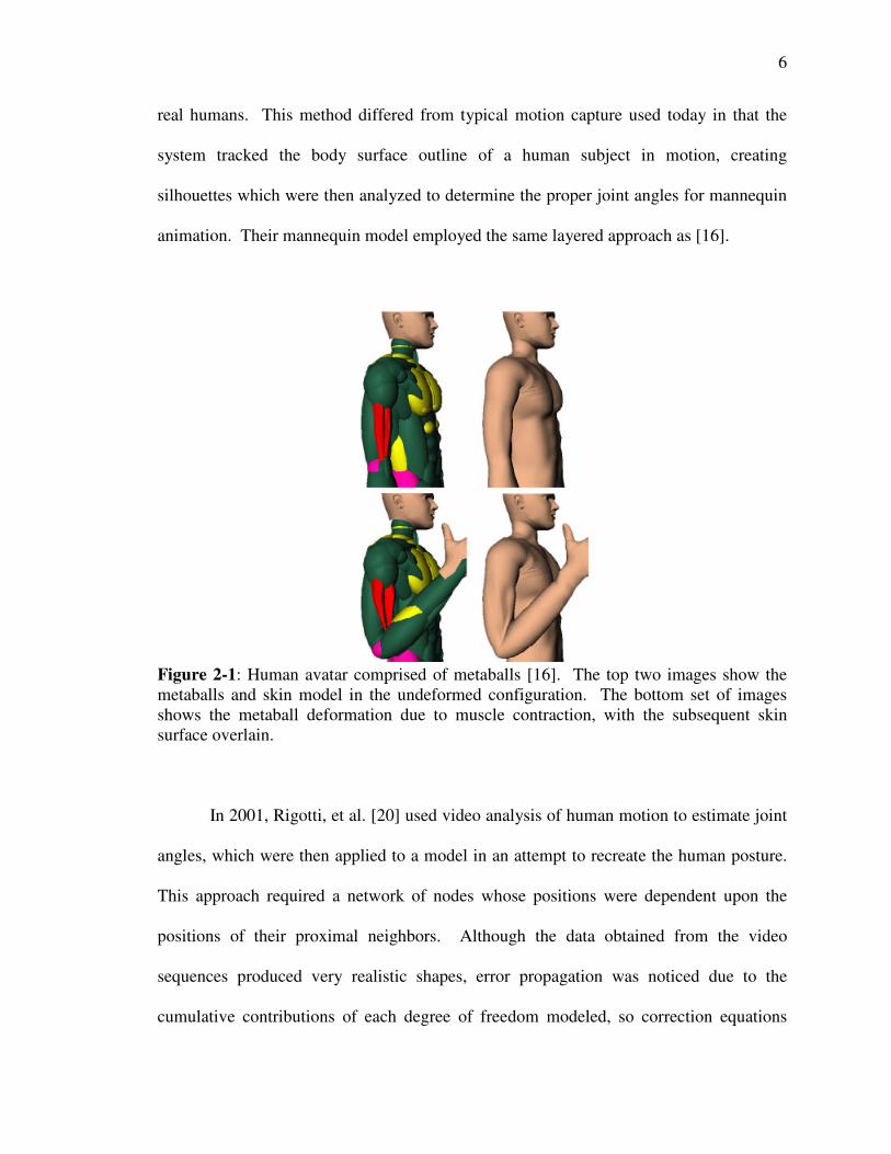
Others have avoided the need for 3D scans altogether by artificially creating their
virtual humans. For example, Nedel and Thalmann [16] developed an entire mannequin
by modeling the bones, muscles, and fatty tissue with ellipsoids and “metaballs,” over
which the skin would then be generated using a cubic B-spline. They employed a muscle
model that deformed in accordance with bone movement, which then resulted in a
deformed skin surface (see Fig. 2-1).
Research in mannequin animation is also a recent venture, coinciding with the
ability of computers to perform the necessary calculations reasonably quickly. For
example, Fua, et al. [4] animated mannequins through the analysis of video sequences of
6
real humans. This method differed from typical motion capture used today in that the
system tracked the body surface outline of a human subject in motion, creating
silhouettes which were then analyzed to determine the proper joint angles for mannequin
animation. Their mannequin model employed the same layered approach as [16].
Figure 2-1: Human avatar comprised of metaballs [16]. The top two images show the
metaballs and skin model in the undeformed configuration. The bottom set of images
shows the metaball deformation due to muscle contraction, with the subsequent skin
surface overlain.
In 2001, Rigotti, et al. [20] used video analysis of human motion to estimate joint
angles, which were then applied to a model in an attempt to recreate the human posture.
This approach required a network of nodes whose positions were dependent upon the
positions of their proximal neighbors. Although the data obtained from the video
sequences produced very realistic shapes, error propagation was noticed due to the
cumulative contributions of each degree of freedom modeled, so correction equations
7
were developed to mitigate the error. Only the spine and a single arm were modeled in
this work.
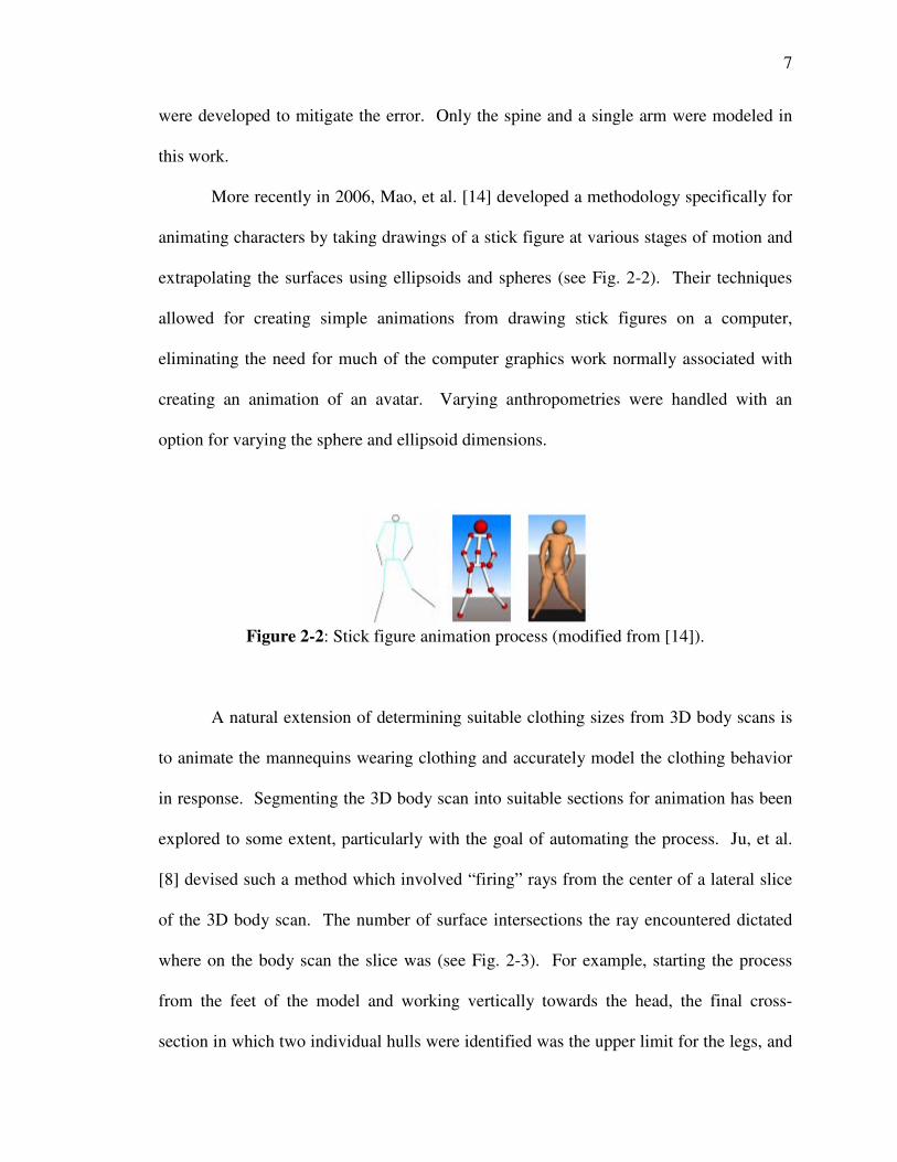
More recently in 2006, Mao, et al. [14] developed a methodology specifically for
animating characters by taking drawings of a stick figure at various stages of motion and
extrapolating the surfaces using ellipsoids and spheres (see Fig. 2-2). Their techniques
allowed for creating simple animations from drawing stick figures on a computer,
eliminating the need for much of the computer graphics work normally associated with
creating an animation of an avatar. Varying anthropometries were handled with an
option for varying the sphere and ellipsoid dimensions.
Figure 2-2: Stick figure animation process (modified from [14]).
A natural extension of determining suitable clothing sizes from 3D body scans is
to animate the mannequins wearing clothing and accurately model the clothing behavior
in response. Segmenting the 3D body scan into suitable sections for animation has been
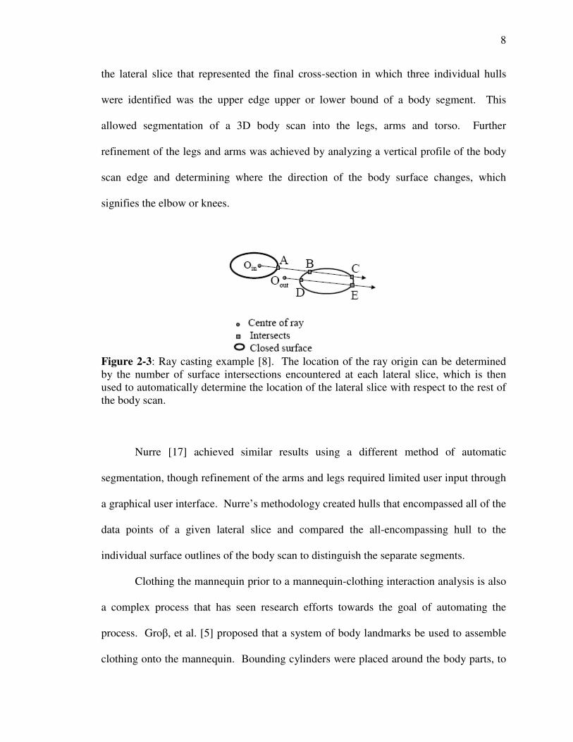
explored to some extent, particularly with the goal of automating the process. Ju, et al.
[8] devised such a method which involved “firing” rays from the center of a lateral slice
of the 3D body scan. The number of surface intersections the ray encountered dictated
where on the body scan the slice was (see Fig. 2-3). For example, starting the process
from the feet of the model and working vertically towards the head, the final cross-
section in which two individual hulls were identified was the upper limit for the legs, and
8
the lateral slice that represented the final cross-section in which three individual hulls
were identified was the upper edge upper or lower bound of a body segment. This
allowed segmentation of a 3D body scan into the legs, arms and torso. Further
refinement of the legs and arms was achieved by analyzing a vertical profile of the body
scan edge and determining where the direction of the body surface changes, which
signifies the elbow or knees.
Figure 2-3: Ray casting example [8]. The location of the ray origin can be determined
by the number of surface intersections encountered at each lateral slice, which is then
used to automatically determine the location of the lateral slice with respect to the rest of
the body scan.
Nurre [17] achieved similar results using a different method of automatic
segmentation, though refinement of the arms and legs required limited user input through
a graphical user interface. Nurre’s methodology created hulls that encompassed all of the
data points of a given lateral slice and compared the all-encompassing hull to the
individual surface outlines of the body scan to distinguish the separate segments.
Clothing the mannequin prior to a mannequin-clothing interaction analysis is also
a complex process that has seen research efforts towards the goal of automating the
process. Groβ, et al. [5] proposed that a system of body landmarks be used to assemble
clothing onto the mannequin. Bounding cylinders were placed around the body parts, to

9
which the garment pieces would be fit and virtually sewn together as necessary.
Garments were placed into one of four categories, each using specific sets of landmarks
to properly place the garment onto the mannequin.
Despite significant advances in clothing modeling in terms of both realism of the
mannequin and the clothing behavior, very little work has been reported on the resistance
that clothing forces onto the wearer. Man, et al. [13] successfully modeled the resistance
a pair of pants exerts on a mannequin when walking and stepping over an obstacle, with
the mannequin represented by ellipsoids and animated via motion capture data (see Fig.
2-4). The clothing was modeled as an elastic medium comprised of shell finite elements
undergoing frictional contact with the ellipsoidal body segments. The clothing contact
forces on the ellipsoids were resolved into mannequin joint torques.
Figure 2-4: Mannequin animation snapshots [13]. The lower body was modeled solely
using ellipsoids and animated with motion capture data.
Seo, et al. [21] looked at the pressure exerted by tight-fitting clothing onto
various-sized mannequins derived from body scans, with the clothing modeled as a mass-
spring system. The model was validated by comparing the results of a simulation to real

10
measurements of the pressure exerted by cloth onto a cylinder. It is noted that the work
of Seo, et al. [21] did not involve an animated mannequin and the work of Man, et al.
[11] modeled the mannequin with simple ellipsoids and not a realistic human body scan.
A variety of research has been reviewed and presented here, offering different
methods of accomplishing the same goals being explored in this thesis, as well as
investigation of research areas that could benefit from the work presented in this thesis.
This review serves as a good departure point and helps to explain why the methods used
herein were chosen by the author, and how these methods relate to others used in the past.

11
CHAPTER 3
BODY SCAN PREPARATION
3.1 Body Scan Composition
The body scans used herein were obtained via laser scan devices at the Cornell
University College of Human Ecology operated by Prof. Susan Ashdown. An initial scan
was obtained in July of 2006 on “Bob” and a later scan was obtained in November of
2007 on “Lisa.” Between the two scans, the laboratory upgraded its scanner to the NX16
model produced by TC-Squared of Cary, NC. The NX16 is capable of scanning a human
subject complete in 8 seconds, with accuracies within 1mm for a single point and 3mm
circumferentially, and resolving up to 1 million points [24].
For ease of implementing the procedures outlined in this thesis, it is important that
the body scan be obtained such that the following three defining body features each be
aligned with a global coordinate system axis: the scan subject frontal direction, the lateral
direction (defined by a segment between the two shoulders), and the vertical direction
(the direction of the subject height). Although the specific axis that corresponds to each
of these three major body axes is not important, the same three axes must be aligned with
the global coordinate system in some manner in order to implement the procedures
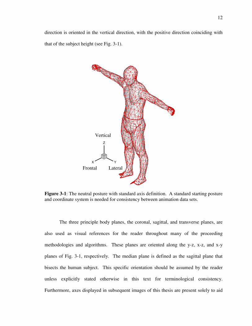
outlined henceforth. In this thesis, the x-axis is chosen arbitrarily to coincide with the
frontal direction, with the positive direction coinciding with the viewing direction of the
subject, the y-axis is chosen as aligned with the lateral direction, with the positive
direction defined from the right shoulder to the left shoulder of the subject, and the z-
12
direction is oriented in the vertical direction, with the positive direction coinciding with
that of the subject height (see Fig. 3-1).
Figure 3-1: The neutral posture with standard axis definition. A standard starting posture
and coordinate system is needed for consistency between animation data sets.
The three principle body planes, the coronal, sagittal, and transverse planes, are
also used as visual references for the reader throughout many of the proceeding
methodologies and algorithms. These planes are oriented along the y-z, x-z, and x-y
planes of Fig. 3-1, respectively. The median plane is defined as the sagittal plane that
bisects the human subject. This specific orientation should be assumed by the reader
unless explicitly stated otherwise in this text for terminological consistency.
Furthermore, axes displayed in subsequent images of this thesis are present solely to aid
Lateral
Vertical
Frontal
13
the reader in gaining a 3D perspective of the image and are therefore unlabeled. Finally,
the location of the origin of the global coordinate axes is arbitrary, though for
convenience it is suggested that it be placed such that all model coordinates are non-
negative.
The scanning software provided by TC-Squared is capable of providing the body
scan data in multiple formats. Due to the author’s familiarity with the AutoCAD
software, the files were obtained in the Drawing Interchange Format (DXF), allowing for
easy manipulation of the body scans for the purposes of this research. The body scan
data itself is given as nodal coordinates and 3D faces in the form of triangular polygons,
though AutoCAD defines 3D faces in terms of 4 nodal coordinates, meaning that the 3rd
and 4th
coordinates of each 3D face are identical in this case. Subsequently, software
written for this thesis is capable of handling 3-noded and 4-noded polygons.
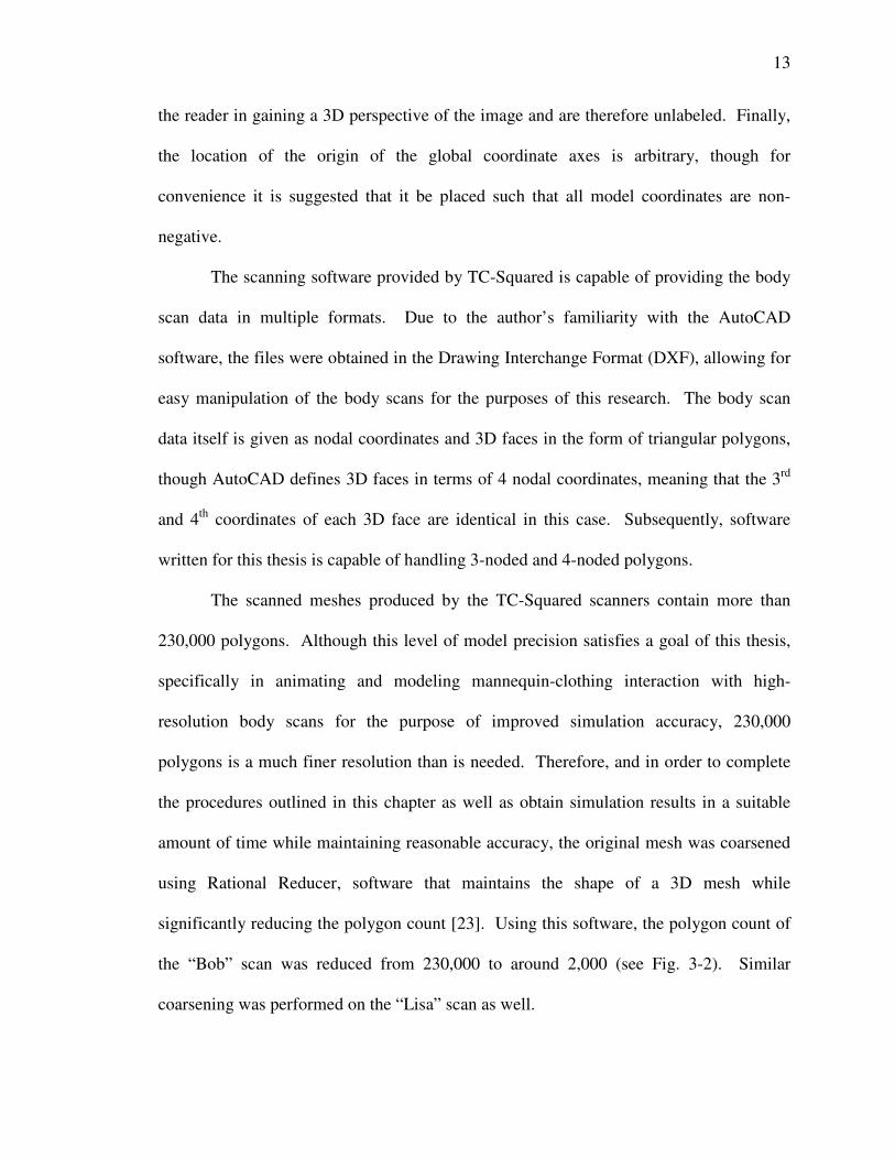
The scanned meshes produced by the TC-Squared scanners contain more than
230,000 polygons. Although this level of model precision satisfies a goal of this thesis,
specifically in animating and modeling mannequin-clothing interaction with high-
resolution body scans for the purpose of improved simulation accuracy, 230,000
polygons is a much finer resolution than is needed. Therefore, and in order to complete
the procedures outlined in this chapter as well as obtain simulation results in a suitable
amount of time while maintaining reasonable accuracy, the original mesh was coarsened
using Rational Reducer, software that maintains the shape of a 3D mesh while
significantly reducing the polygon count [23]. Using this software, the polygon count of
the “Bob” scan was reduced from 230,000 to around 2,000 (see Fig. 3-2). Similar
coarsening was performed on the “Lisa” scan as well.
14
Figure 3-2: Mesh coarsening comparison. The mesh on the left has over 230,000
polygons, whereas the mesh on the right has only 2,000 while still maintaining a visually
similar surface geometry.
3.2 Body Scan Reconstruction
Although the laser body scanning system is a fast and accurate way to obtain body
scans, it presently limited by its ability to scan surfaces that are parallel or near-parallel
with the scanning laser. This leads to gaps in the mesh at surface locations such as the
tops of shoulders, feet, and head of the subject. Such holes in the mesh are increasingly
more tedious to fix the finer the mesh resolution as more polygons would be needed to
patch the gaps. No automatic patching algorithms were used in this research for
simplicity and because of the inherent problems in them that will be discussed later in
this chapter, and manual patching was not performed until the mesh was coarsened (recall
Fig. 3-2), significantly reducing the number of polygons that needed to be manipulated to

15
repair and segment the mannequin mesh. Indeed, after mesh coarsening, the majority of
gaps in the body scan mesh were easily replaced with only a few polygons.
In addition to the difficulties in scanning lateral surfaces, the dimensions of space
that can be scanned are limited to about the size of a telephone booth. If the subject were
to be scanned with the arms fully outstretched (in the neutral posture), part of the arms
would protrude from the scanning volume. This forces the scanning subject to keep the
arms angled downwards (recall Fig. 3-2), and therefore requires that the mesh be
manipulated to fully extend the arms laterally to achieve the neutral posture. In the
future, having a standard posture that applies to both scan subjects and animation data set
would ensure compatibility between the two and expedite the alignment process
presented in Chapter 4.
Typically, the only portion of the body that needs to be realigned to fit the neutral
position is the arms, and this can easily be achieved by locating the approximate joint
center of each shoulder and rotating the respective arms about this point until they are
pointed directly outward in the lateral direction; naturally, this rotation would occur
within the coronal plane. Locating the joint center of the shoulders with high precision is
not necessary as the area around the shoulders will need to be repaired regardless due to
the aforementioned unscannable surfaces and because the mesh polygons near the
shoulder will no longer be plum.
For a number of reasons, scanners have difficulty capturing the body surface
geometry around the shoulders. Two such reasons for this difficulty are that the top of
the shoulders are nearly level with the scan direction, as previously mentioned. Another
is that the arms themselves obstruct the line of sight of the scanner to the armpit region.

16
These difficulties in scanning the shoulder and armpit region of the human body
necessitate patching and repair of the body scan. In repairing and patching the body scan
in this region, the gross symmetry that exists in the human subject should be preserved.
To accomplish this goal, a systematic procedure was developed to restore the symmetry
of a mannequin at the shoulders, based upon the global coordinate system alignment
suggested at the beginning of this chapter.
The shoulder with the most complete mesh (the one with the smallest portion of
mesh missing) is subjectively chosen to become the “prototype” and will be used to
reconstruct the opposing shoulder via cloning and mirroring. It is not necessary that the
more complete shoulder be selected as the prototype, but doing so will shorten the length
of time required to finish the proceeding patching and repair methodology. Fig. 3-3
shows the completed shoulder (the right shoulder, in this case) being used to reconstruct
the opposite shoulder in the following example. When the shoulder is complete on one
side, it will be delimited by a set of nodes forming a boundary between one body segment
(the torso) and the next (an arm) in the shape of a roughly circular opening, referred to in
this section as the shoulder boundary. The nodes defining the shoulder boundary will be
referred to as shoulder boundary nodes. When the individual sections of the body
produced by segmentation are formally introduced as body segments later in this chapter,
these boundaries will be referred to as body segment edges.
The shoulder boundary delimitation for the prototype shoulder will lie in a sagittal
plane a certain distance away from the medial plane of the body scan mesh. When
reconstructing the mesh of the opposing shoulder, the new shoulder boundary will be a
mirror image of the prototype’s shoulder boundary and will lie in a sagittal plane the

17
same distance removed from the medial plane as the prototype. To begin the symmetry
reconstruction, rays are extended laterally from each of the prototype shoulder’s
boundary nodes toward the boundary sagittal plane of the opposing shoulder. If the
mannequin is scanned with the global axes as shown in Fig. 3-1, these rays will be along
the global y-axis, or in the lateral direction. The intersection of these rays with the
sagittal plane at the shoulder-arm transition of the incomplete shoulder (see Fig. 3-4)
forms the basis of the new shoulder cross-section (see Fig. 3-5). In this case incomplete
shoulder had a wider boundary (opening at the upper arm) than that of the complete
shoulder. The new shoulder boundary, shown in Fig. 3-5, is created by connecting the
shoulder boundary nodes by a sequence of line segments in the sagittal plane.
Figure 3-3: The complete right shoulder being used to reconstruct the incomplete scan of
the left shoulder. The shoulder boundary shown lies in a sagittal plane and its mirror
image will lie in a similar plane. Rays are extended laterally from each shoulder node
through the sagittal plane of the opposing shoulder. The prototype shoulder edge and the
edge nodes, from which the shoulder projections are drawn, are highlighted. The
shoulder projections are depicted by the parallel lines, which lie in coronal planes.
18
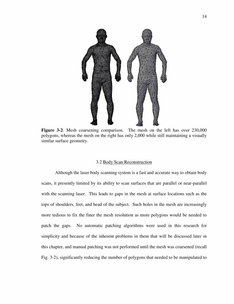
Figure 3-4: Intersection of sagittal plane with body scan at the incomplete shoulder
boundary. The sagittal plane pictured is located at the incomplete shoulder boundary,
where the new shoulder boundary is to be formed based upon projections from the
prototype shoulder.
Figure 3-5: Formation of the new shoulder boundary. The prototype shoulder node
extensions are again depicted as the parallel lines, with a portion of the new shoulder
boundary represented by the dashed line. The first three nodes that will comprise the new
shoulder opening are highlighted with square symbols.
19
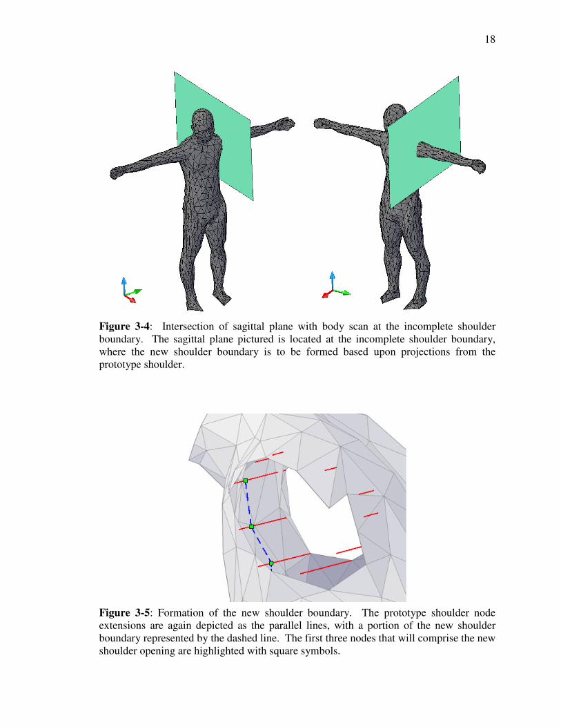
Because the new shoulder boundary lies within a sagittal plane, the comprising
line segments, which will later become polygon edges of the new shoulder, are
perpendicular to the lateral direction. Thus, creation of the new shoulder boundary that
defines the upper arm opening only requires knowing the intersection points between a
sagittal plane at the new shoulder and the lateral rays extended from the shoulder
boundary nodes of the prototype shoulder. Ideally, the location of the sagittal plane in
which the reconstructed shoulder boundary will reside should be the same distance from
the medial plane of the body scan as that of the prototype shoulder. In actuality, this can
be estimated by the user to achieve gross symmetry. Once the boundary of the to-be-
reconstructed shoulder has been completed, as shown in Fig. 3-6, the next step is to
reshape the torso portion of the mesh to conform to it.
Figure 3-6: Completed shoulder boundary extrapolation. The completed boundary is
represented by the dashed line. The vertices of the new shoulder boundary are
highlighted by square symbols, and the shoulder node extensions are depicted by solid,
parallel lines. The new shoulder boundary occurs at the intersection between the
shoulder node extensions and the mirrored sagittal plane (recall Fig. 3-4).
20
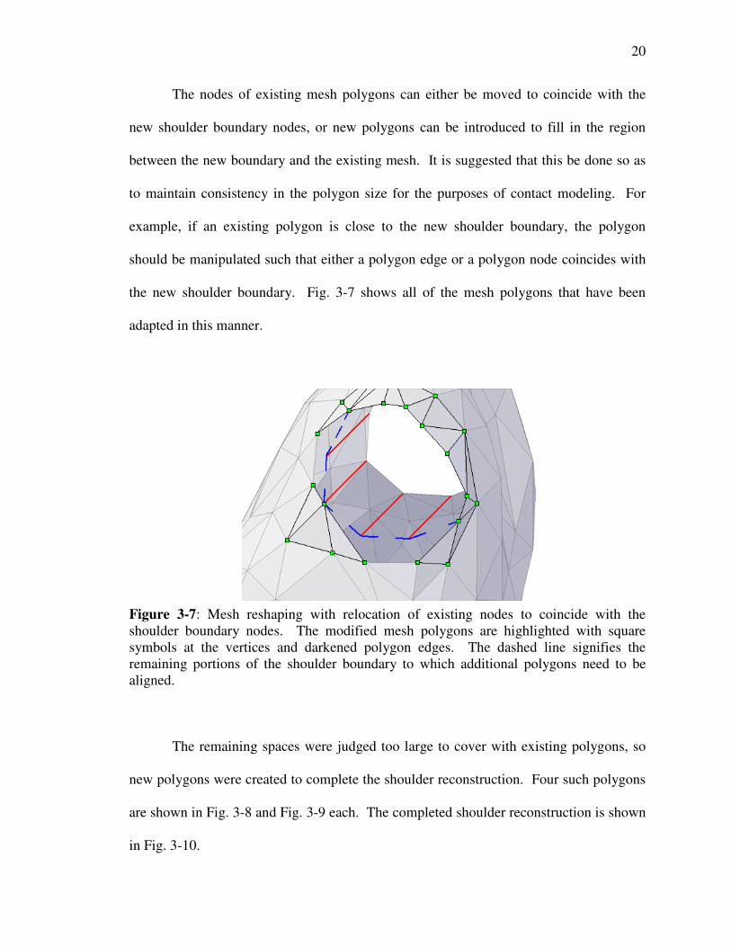
The nodes of existing mesh polygons can either be moved to coincide with the
new shoulder boundary nodes, or new polygons can be introduced to fill in the region
between the new boundary and the existing mesh. It is suggested that this be done so as
to maintain consistency in the polygon size for the purposes of contact modeling. For
example, if an existing polygon is close to the new shoulder boundary, the polygon
should be manipulated such that either a polygon edge or a polygon node coincides with
the new shoulder boundary. Fig. 3-7 shows all of the mesh polygons that have been
adapted in this manner.
Figure 3-7: Mesh reshaping with relocation of existing nodes to coincide with the
shoulder boundary nodes. The modified mesh polygons are highlighted with square
symbols at the vertices and darkened polygon edges. The dashed line signifies the
remaining portions of the shoulder boundary to which additional polygons need to be
aligned.
The remaining spaces were judged too large to cover with existing polygons, so
new polygons were created to complete the shoulder reconstruction. Four such polygons
are shown in Fig. 3-8 and Fig. 3-9 each. The completed shoulder reconstruction is shown
in Fig. 3-10.

21
Figure 3-8: Shoulder reshaping with addition of new polygons. The node projections are
depicted by the solid, parallel lines, and the added polygons are highlighted with square
symbols at the vertices and darkened polygon edges. The dashed line represent the
portion of the new shoulder boundary yet to be completed.
Figure 3-9: Shoulder reshaping with the final set of polygon additions. The node
projections are depicted by the solid, parallel lines and the added polygons are
highlighted with square symbols at the vertices and darkened polygon edges. The
polygons highlighted comprise the final part of the new shoulder boundary, completing
the reconstruction procedure.

22
Figure 3-10: Completed reconstruction of the shoulder. The shoulder boundary nodes
are highlighted with square symbols at the vertices and a darkened border over the
boundary. This boundary coincides with the intersection of the sagittal plane and the
body scan mesh depicted in Fig. 3-4.
With gross shoulder symmetry obtained through reconstruction, the meshes of
both upper arms should be repaired. The same procedure used in reshaping the shoulder
mesh around the shoulder boundary should be used here in reshaping the upper arm
mesh. This again requires a decision on whether to create new polygons or to move the
nodes of existing polygons to conform to the upper arm boundaries. This procedure is
sufficient for the upper surface of the arms as the gap is typically small. The gap in the
armpit region, however, is comparatively large and thus requires a new procedure for
repair.
The underarm portions of the mesh can be extrapolated to completeness in much
the same way that the shoulder was reconstructed to provide symmetry via node
projections. First, one must identify nodes on both the upper arm boundary and shoulder
boundary that define body scan mesh contour changes
surface shape-identifying (SSI)
boundary node to be an SSI node is that it not be collinear with its two adjacent nodes
(see Fig. 3-11). The nodes on the boundary of the incomplete portion of the upper arm
mesh are then connected to suitable SSI nodes of the
segments that will serve as the contour edges for the new underarm shape (see Fig. 3
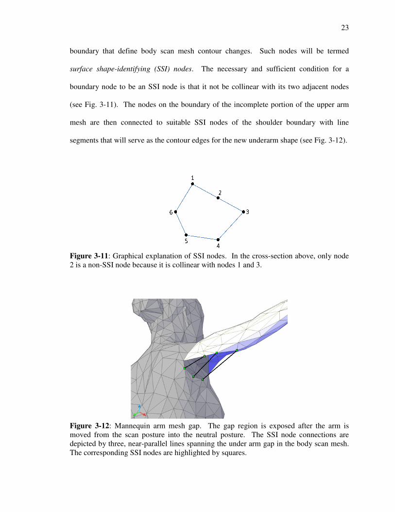
Figure 3-11: Graphical explanation of SSI nodes. In the
2 is a non-SSI node because it is collinear
Figure 3-12: Mannequin arm mesh gap. Th
moved from the scan posture
depicted by three, near-parallel lines spanning the under arm gap
The corresponding SSI nodes are highlighted by squares.
fine body scan mesh contour changes. Such nodes will be termed
identifying (SSI) nodes. The necessary and sufficient condition for a
boundary node to be an SSI node is that it not be collinear with its two adjacent nodes
The nodes on the boundary of the incomplete portion of the upper arm
mesh are then connected to suitable SSI nodes of the shoulder boundary with line
segments that will serve as the contour edges for the new underarm shape (see Fig. 3
: Graphical explanation of SSI nodes. In the cross-section above, only node
SSI node because it is collinear with nodes 1 and 3.
: Mannequin arm mesh gap. The gap region is exposed after the arm is
posture into the neutral posture. The SSI node connections are
parallel lines spanning the under arm gap in the body scan mesh.
The corresponding SSI nodes are highlighted by squares.
23
Such nodes will be termed
sufficient condition for a
boundary node to be an SSI node is that it not be collinear with its two adjacent nodes
The nodes on the boundary of the incomplete portion of the upper arm
shoulder boundary with line
segments that will serve as the contour edges for the new underarm shape (see Fig. 3-12).
section above, only node
region is exposed after the arm is
ture. The SSI node connections are
in the body scan mesh.
24
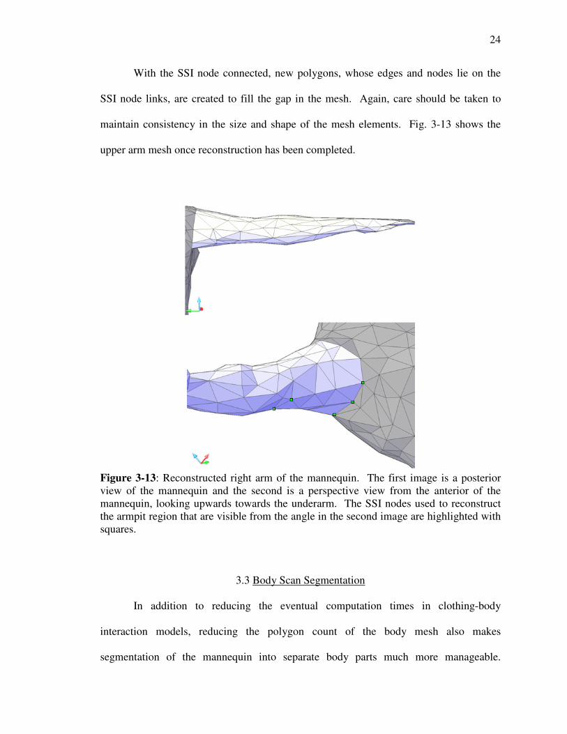
With the SSI node connected, new polygons, whose edges and nodes lie on the
SSI node links, are created to fill the gap in the mesh. Again, care should be taken to
maintain consistency in the size and shape of the mesh elements. Fig. 3-13 shows the
upper arm mesh once reconstruction has been completed.
Figure 3-13: Reconstructed right arm of the mannequin. The first image is a posterior
view of the mannequin and the second is a perspective view from the anterior of the
mannequin, looking upwards towards the underarm. The SSI nodes used to reconstruct
the armpit region that are visible from the angle in the second image are highlighted with
squares.
3.3 Body Scan Segmentation
In addition to reducing the eventual computation times in clothing-body
interaction models, reducing the polygon count of the body mesh also makes
segmentation of the mannequin into separate body parts much more manageable.

25
Segmentation, as alluded to earlier, is the process by which a body scan is separated into
specific, well-defined entities (see Fig. 3-14 for a diagram of the body segment names
and locations used in this research). Each of these segments spans major joints of the
body and will eventually be animated with a set of 3 data points each, termed control
points, to produce a fully-animated mannequin. Each body segment is bounded by one or
more body segment edges, located at the mannequin-equivalent locations of human body
joints, and are closed curves analogous to the shoulder boundaries and the upper arm
boundaries discussed in the previous section (see Fig. 3-15 for body segment edge names
and locations used in this research).
Figure 3-14: Diagram of body segments. All body segments are animated independently
except for the hands, feet, and head, which are animated in tandem with their adjacent
body segments. The hands are animated with their respective adjacent lower arm
segments, the feet with their respective adjacent lower leg segments, and the head with
the torso segment.
Right Upper Arm Left Upper Arm
Head
Torso
Left Hand
Right Hand
Right Foot Left Foot
Right Lower Leg
Right Upper Leg
Left Lower Arm Right Lower Arm
Left Lower Leg
Left Upper Leg
Pelvis
26
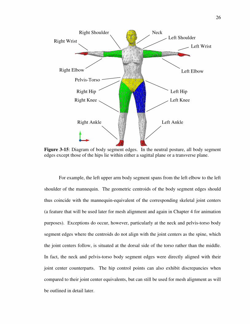
Figure 3-15: Diagram of body segment edges. In the neutral posture, all body segment
edges except those of the hips lie within either a sagittal plane or a transverse plane.
For example, the left upper arm body segment spans from the left elbow to the left
shoulder of the mannequin. The geometric centroids of the body segment edges should
thus coincide with the mannequin-equivalent of the corresponding skeletal joint centers
(a feature that will be used later for mesh alignment and again in Chapter 4 for animation
purposes). Exceptions do occur, however, particularly at the neck and pelvis-torso body
segment edges where the centroids do not align with the joint centers as the spine, which
the joint centers follow, is situated at the dorsal side of the torso rather than the middle.
In fact, the neck and pelvis-torso body segment edges were directly aligned with their
joint center counterparts. The hip control points can also exhibit discrepancies when
compared to their joint center equivalents, but can still be used for mesh alignment as will
be outlined in detail later.
Left Ankle Right Ankle
Left Knee Right Knee
Right Hip Left Hip
Right Wrist
Right Shoulder
Right Elbow Left Elbow
Left Shoulder
Left Wrist
Neck
Pelvis-Torso

For the purposes of animation,
animated body segments: the torso (includes the
(includes the hands), the two upper arms, the pelvis, the two upper legs, and the two
lower legs (includes the feet).
animation algorithm used herein crates gaps that can
get caught between segments during simulation
such as skinning, a generic term for any process through which gaps in the mesh are
covered by the creation and manipulation of polygons over and near the animation
created gaps, will create unnecessary complexity in the model and potential problems
with contact modeling algorithms,
overlaps was developed.
formation of easily-patchable,
patching techniques. For example, when the
relative rotations about the
shape of an arc (see Fig. 3
geometries such as spheres and ellipsoids.
Figure 3-16: Example of an arc
about the joint centroid with respect to
For the purposes of animation, the mannequin is composed of ten
body segments: the torso (includes the neck and head), the two lower arms
ds), the two upper arms, the pelvis, the two upper legs, and the two
lower legs (includes the feet). The rigid body motion assumption utilized in the
animation algorithm used herein crates gaps that cannot be ignored as t
segments during simulation. Employing time-consuming solutions
, a generic term for any process through which gaps in the mesh are
covered by the creation and manipulation of polygons over and near the animation
will create unnecessary complexity in the model and potential problems
with contact modeling algorithms, so a simple method of patching these gaps and
overlaps was developed. The choice of segmentation presented herein
tchable, arc-shaped gaps, thereby avoiding use of more complex
. For example, when the upper and lower arm segments undergo
relative rotations about the elbow body segment edge, a gap will be created
3-16). Such arc-shaped gaps will allow for patching with simple
geometries such as spheres and ellipsoids.
: Example of an arc-shaped gap. This gap is created as one segment rotates
about the joint centroid with respect to an adjacent segment.
27
ten independently-
head), the two lower arms
ds), the two upper arms, the pelvis, the two upper legs, and the two
The rigid body motion assumption utilized in the
the clothing may
consuming solutions
, a generic term for any process through which gaps in the mesh are
covered by the creation and manipulation of polygons over and near the animation-
will create unnecessary complexity in the model and potential problems
so a simple method of patching these gaps and
presented herein promotes the
, thereby avoiding use of more complex
segments undergo
created having the
will allow for patching with simple
as one segment rotates
28
Because the mannequin model assumes rigid body motion, the mesh surface does
not adjust to conform to new shapes brought about during animation, thereby forming the
previously-mentioned gaps in the mesh surface during animation. The desire to create
arc-shaped gaps during the animation is used as a guideline in determining the
configuration of the body segment edges. Investigation revealed that the body segment
edge configuration presented in Figures 3-14 and 3-15 is a good solution for creating the
desired gap curves during animation. To this end, with the mannequin in the neutral
posture, the elbow, wrist, and shoulder body segment edges are aligned with the sagittal
plane, and the neck, torso-pelvis joint, knee, and ankle body segment edges are aligned
laterally.
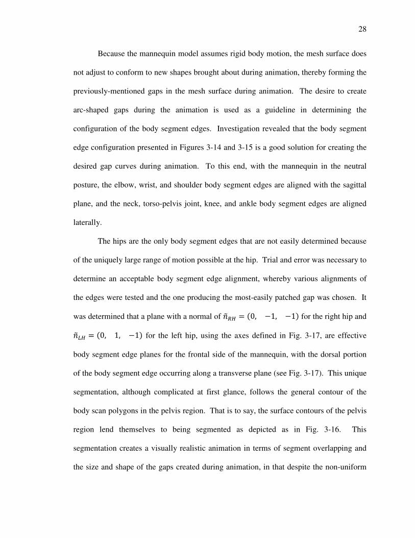
The hips are the only body segment edges that are not easily determined because
of the uniquely large range of motion possible at the hip. Trial and error was necessary to
determine an acceptable body segment edge alignment, whereby various alignments of
the edges were tested and the one producing the most-easily patched gap was chosen. It
was determined that a plane with a normal of �� = �0, −1, −1� for the right hip and
��� = �0, 1, −1� for the left hip, using the axes defined in Fig. 3-17, are effective
body segment edge planes for the frontal side of the mannequin, with the dorsal portion
of the body segment edge occurring along a transverse plane (see Fig. 3-17). This unique
segmentation, although complicated at first glance, follows the general contour of the
body scan polygons in the pelvis region. That is to say, the surface contours of the pelvis
region lend themselves to being segmented as depicted as in Fig. 3-16. This
segmentation creates a visually realistic animation in terms of segment overlapping and
the size and shape of the gaps created during animation, in that despite the non-uniform
29
body segment edge the two hip body segment edges can be patched with a single
ellipsoid at each hip.
Figure 3-17: Front (right) and rear (left) view of the pelvis segment. The pelvis body
segment is the middle segment in both views. Animations of the two models made using
this segmentation yielded visually accurate results in both the legs, pelvis, and buttocks.
The division of the body scan mesh into the aforementioned segments is
performed by creating planes of the necessary orientation through the desired body
segment edge locations of the body scan mesh, exactly as was done with the shoulder
symmetry reconstruction outlined earlier (recall Fig. 3-4). The mesh polygons that
intersect with the planes are then either divided to create polygon edges conforming to
the new body segment edge or, if the polygon nodes of the neighboring body segment
edges are close enough to the plane to warrant it, the nodes are moved to lie concurrent
with the planes designating the body segment edges. Similar judgment as was used
during the shoulder reshaping procedure regarding whether a new polygon is needed or
current ones can be modified during shoulder reshaping was used for this procedure.
Y
�� ���
X
Z

30
AutoCAD was again the 3D modeling software chosen by the author to complete the
segmentation procedure.
A key advantage of the segmentation methodology presented in this thesis is that
it avoids the commonly used solution of skinning. Skinning techniques are often
automated in that little to no user input is required, particularly when compared to the
methodologies presented in this thesis for accomplishing the same tasks; however,
utilization of skinning to patch animation gaps in the mesh is avoided as it can create
complications during contact modeling because the number of polygons, nodes, and their
respective alignments and ordering can change between time steps in the animation due
to the manipulation of the mesh inherent with skinning. In addition, the skinning process
adds computation time as new surface geometries must be updated at each time step. In
the case of the contact algorithm of [11], a morphing surface geometry can lead to
problems during mannequin-clothing interaction models whereby the mannequin mesh
polygon nearest a clothing surface node may change too quickly for the contact algorithm
to compensate.
Furthermore, although a few algorithms have been presented to automatically
segment virtual mannequins, each presents its own flaws if extended for use in this
research, particularly in creating the need for skinning rather than the simple approach
presented later in this chapter, whereby spheres and ellipsoids are used to patch animation
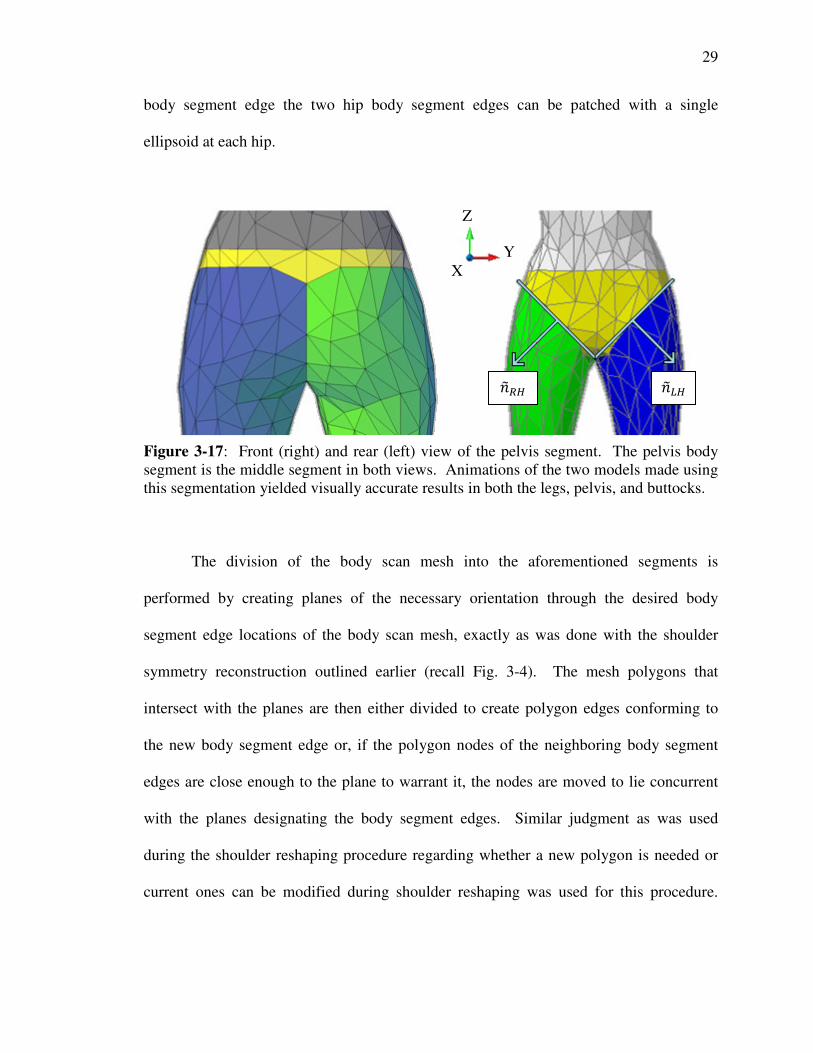
gaps. An example of such a potentially-problematic automatic segmentation algorithm is
the work in [8] presented earlier and depicted in Fig. 3-18, as it creates an undesirable
situation at the shoulders and pelvis, where the automated segmentation occurs laterally.
For small arm and leg movements (relative to their initial positions) this is acceptable as
31
little overlapping of segments occurs and the gaps formed are very small and therefore do
not require advanced patching techniques such as skinning. However, when the
appendages undergo a wider range of motion, this can cause the segments to intersect
with each other or create unnatural or large gaps between segments that would require
skinning or some other mesh-adjusting algorithm due to the oddity of the gaps or
overlaps created.
Figure 3-18: Ray casting automated segmentation result [8]. The horizontal transitions
between the torso, arms, and legs make it difficult to animate the mannequin without
experiencing significant overlap or gaps that are difficult to patch without more complex
methods.
3.4 Spherical and Ellipsoidal Joint Segments
As previously mentioned, a simple-yet-effective solution is needed to prevent the
clothing from getting caught between segments during analysis, while maintaining as
much of a visual realism in the animation as possible. In other words, the solution needs
to have the patching elements present at all time, but only to appear or become operative
when gaps are formed due to relative movement of the body segments. The method
32
chosen for fulfilling these goals is to use ellipsoids and spheres that are animated in
tandem with the body segments they are meant to patch.
Spheres are placed at joints with circular-shaped cross-sections (e.g. the elbow
and knee body segment edges), and ellipsoids placed at the joints with ellipsoidal-shaped
cross-sections (e.g. the pelvis-torso and hip body segment edges). The placement of both
the ellipsoids and spheres were found to work well when located at the body segment
edge centroids. The radius of the spheres were be taken as the average distance between
opposing nodes in the circular cross-section (see Fig. 3-19), and the ellipsoid dimensions
were determined by taking the maximum and minimum distances between opposing
nodes in the cross-section (see Fig. 3-20). The third ellipsoid dimension is generally
chosen to be the size of the aforementioned minimum distance, creating a circular cross-
section to the ellipsoid, though a wider range of values will also work effectively and will
be presented shortly. The necessary patch dimensions mentioned above can be easily
obtained from a 3D modeling program, such as AutoCAD, as was done in this research.
Although placement of each of these spheres and ellipsoids at the segment joint
centroids is generally a good solution, it does not work well for the hips. That is, the
centroid of the hip body segment edges provide a good approximation of the vertical and
frontal coordinates for placement of the ellipsoid patch, but the patches may need to be
situated closer towards the medial plane so as to minimize extrusion of the ellipsoids
outside of the mannequin mesh. The hip ellipsoid patches have a circular cross-section in
the transverse plane; however, the vertical dimension of the hip body segment edge is
significantly larger than the other two dimensions, thus requiring an ellipsoid to be used
as a patch at the hips to adequately cover any gaps formed during animation, namely at
the mannequin posterior. In other words, the major axis of these ellipsoidal patches will
be positioned vertically, with the other two dimensions of the e
thereby creating the circular cross
ellipsoid patch at pelvis
ellipsoid oriented laterally.
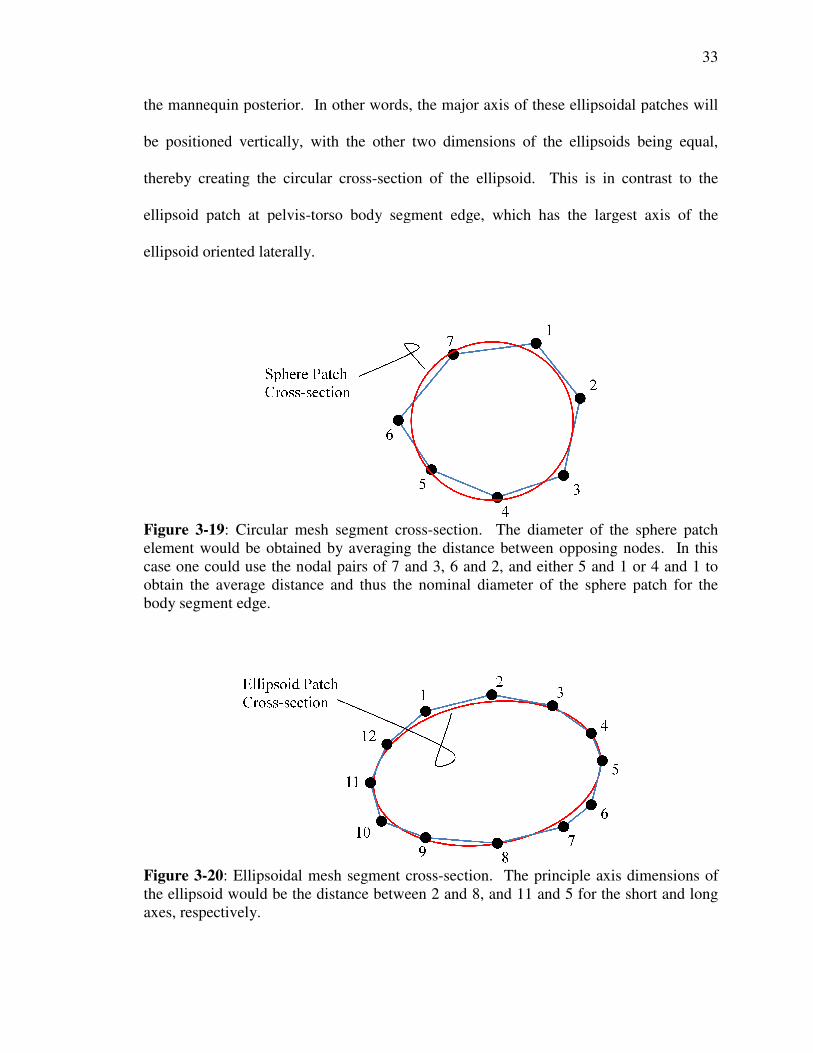
Figure 3-19: Circular mesh segment cross
element would be obtained by averaging the distance between opposing nodes. In this
case one could use the nodal pairs of 7 and 3, 6 and 2, and either 5 and 1 or 4 and 1 to
obtain the average distance and thus the nominal diameter of the sphere patch for the
body segment edge.
Figure 3-20: Ellipsoidal mesh segment cross
the ellipsoid would be the distance between 2 and 8, and 11 and 5 for the short
axes, respectively.
the mannequin posterior. In other words, the major axis of these ellipsoidal patches will
be positioned vertically, with the other two dimensions of the ellipsoids being equal,
thereby creating the circular cross-section of the ellipsoid. This is in contrast to the
ellipsoid patch at pelvis-torso body segment edge, which has the largest axis of the
ellipsoid oriented laterally.
mesh segment cross-section. The diameter of the sphere patch
element would be obtained by averaging the distance between opposing nodes. In this
nodal pairs of 7 and 3, 6 and 2, and either 5 and 1 or 4 and 1 to
istance and thus the nominal diameter of the sphere patch for the
: Ellipsoidal mesh segment cross-section. The principle axis dimensions of
the ellipsoid would be the distance between 2 and 8, and 11 and 5 for the short
33
the mannequin posterior. In other words, the major axis of these ellipsoidal patches will
llipsoids being equal,
section of the ellipsoid. This is in contrast to the
torso body segment edge, which has the largest axis of the
section. The diameter of the sphere patch
element would be obtained by averaging the distance between opposing nodes. In this
nodal pairs of 7 and 3, 6 and 2, and either 5 and 1 or 4 and 1 to
istance and thus the nominal diameter of the sphere patch for the
section. The principle axis dimensions of
the ellipsoid would be the distance between 2 and 8, and 11 and 5 for the short and long

The pelvis-torso patch
body segment edge (see Fig. 3
ellipsoid patch was found to work well at any value
dimension of the ellipsoid within the transverse plane (using 100% would create a
circular cross-section along a sagittal plane intersecting the ellipsoid)
animation patches, the lateral
span of the hip body segment edges, as
of the ellipsoid patches can be effectively approximated as
vertical span of the pelvis body
Figure 3-21: Frontal view of the pelvis body segment with noted dimensions used for
sizing the animation patches. The dimensions shown are used to gauge the ellipsoid
dimensions of the hips and pelvis
As mentioned previously, the lateral and frontal dimensions of the hip animation
patches are equal. This is because of the inherent circular cross
region of the human body.
and without the sphere and ellipsoid patches.
the shoulders, knees, and hips
torso patches are dimensioned to match the outline of the pelvis
body segment edge (see Fig. 3-21). In addition, the vertical dimension of the pelvis
ellipsoid patch was found to work well at any value between 50-100% of the minor axis
dimension of the ellipsoid within the transverse plane (using 100% would create a
along a sagittal plane intersecting the ellipsoid)
lateral dimension can be effectively approximated as the lateral
span of the hip body segment edges, as viewed from the front, and the vertical dimension
of the ellipsoid patches can be effectively approximated as between 150
pelvis body segment in frontal view (see Fig. 3-21).
: Frontal view of the pelvis body segment with noted dimensions used for
sizing the animation patches. The dimensions shown are used to gauge the ellipsoid
dimensions of the hips and pelvis-torso body segment edge patches.
As mentioned previously, the lateral and frontal dimensions of the hip animation
patches are equal. This is because of the inherent circular cross-section to the thigh
region of the human body. Fig. 3-22 shows a snapshot of a mannequin in
and without the sphere and ellipsoid patches. Significant animation gaps can be seen at
the shoulders, knees, and hips in the unpatched snapshot.
34
are dimensioned to match the outline of the pelvis-torso
he vertical dimension of the pelvis-torso
100% of the minor axis
dimension of the ellipsoid within the transverse plane (using 100% would create a
along a sagittal plane intersecting the ellipsoid). For the hip
ectively approximated as the lateral
and the vertical dimension
between 150-200% of the
: Frontal view of the pelvis body segment with noted dimensions used for
sizing the animation patches. The dimensions shown are used to gauge the ellipsoid
As mentioned previously, the lateral and frontal dimensions of the hip animation
section to the thigh
shows a snapshot of a mannequin in animation, with
Significant animation gaps can be seen at
35
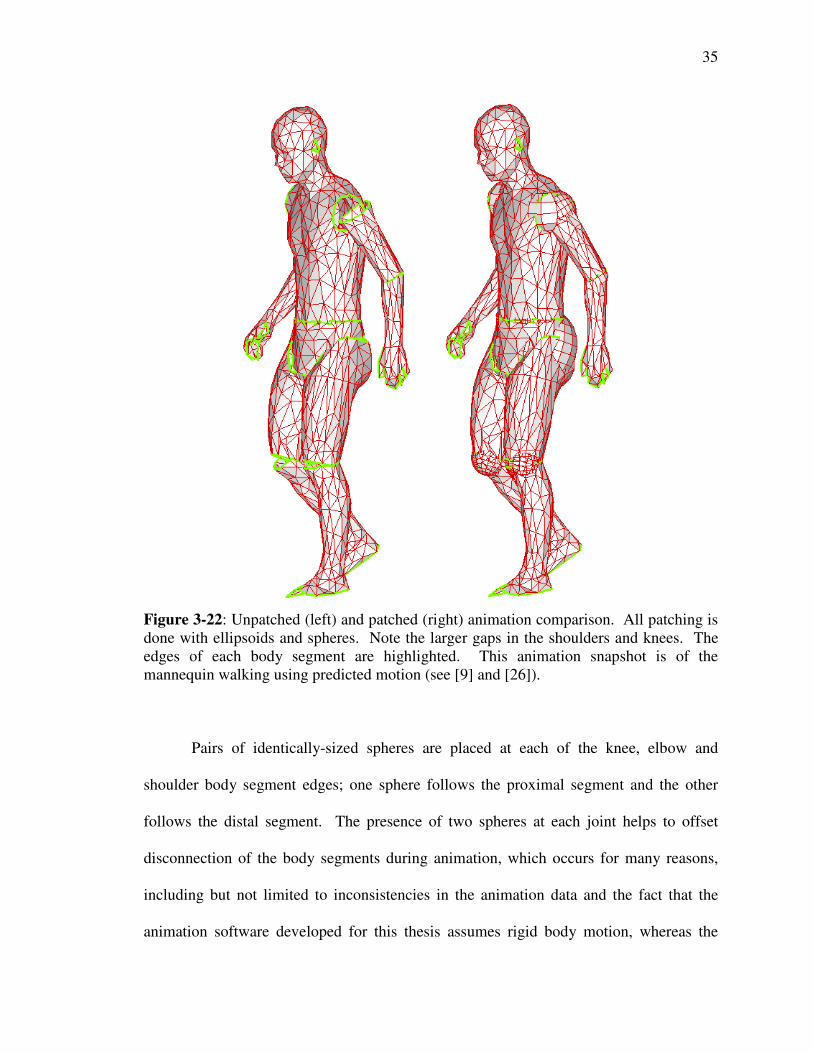
Figure 3-22: Unpatched (left) and patched (right) animation comparison. All patching is
done with ellipsoids and spheres. Note the larger gaps in the shoulders and knees. The
edges of each body segment are highlighted. This animation snapshot is of the
mannequin walking using predicted motion (see [9] and [26]).
Pairs of identically-sized spheres are placed at each of the knee, elbow and
shoulder body segment edges; one sphere follows the proximal segment and the other
follows the distal segment. The presence of two spheres at each joint helps to offset
disconnection of the body segments during animation, which occurs for many reasons,
including but not limited to inconsistencies in the animation data and the fact that the
animation software developed for this thesis assumes rigid body motion, whereas the

human body is more dynamic
motion capture source because of the method by which the data is obtained. Cameras
track reflective balls at strategic locations on the subject during animation. If these
markers are attached to a suit worn by the subject, b
the suit may slip along the skin of the subject and thus
at fixed distances from each other throughout the animation
of the degrees of freedom employed in the mannequin animations for this thesis.
Figure 3-23: Diagram of the degrees of freedom used for mannequin animation. Each
axis of rotation indicated in the diagram represents a degree of freedom
convention implied. Only twenty
group for their DH-driven model
animate a mannequin herein
re dynamic. Animation data inconsistencies typically occur with a
motion capture source because of the method by which the data is obtained. Cameras
track reflective balls at strategic locations on the subject during animation. If these
ched to a suit worn by the subject, because the skin stretches across joints
the suit may slip along the skin of the subject and thus these reflective balls
at fixed distances from each other throughout the animation. Fig. 3-23 shows a diagra
of the degrees of freedom employed in the mannequin animations for this thesis.
: Diagram of the degrees of freedom used for mannequin animation. Each
axis of rotation indicated in the diagram represents a degree of freedom
. Only twenty-one of the 109 degrees of freedom utilized by the VSR
driven model at the time of writing this thesis are employed to
herein.
36
Animation data inconsistencies typically occur with a
motion capture source because of the method by which the data is obtained. Cameras
track reflective balls at strategic locations on the subject during animation. If these
ecause the skin stretches across joints
these reflective balls may not stay
23 shows a diagram
of the degrees of freedom employed in the mannequin animations for this thesis.
: Diagram of the degrees of freedom used for mannequin animation. Each
axis of rotation indicated in the diagram represents a degree of freedom, with no sign
degrees of freedom utilized by the VSR
are employed to

37
Once the body scan mesh is complete, without any sections of mesh missing, the
mannequin properly segmented, and the mannequin patched with simple geometric
shapes, each of the body segment edge centroids of the mannequin can be located so that
the body scan segments can be moved in tandem with animation. This procedure is
discussed in detail in the next chapter along with the data alignment procedure and
algorithms developed to allow the mannequin to be animated via multiple data sources –
namely predictive dynamics data, developed at the University of Iowa by the Virtual
Soldier Research group and based upon a DH kinematics-driven skeletal model, and
motion capture data.
38
CHAPTER 4
VIRTUAL MANNEQUIN ANIMATION
4.1 Orientating the Mannequin Segments
Any animation of a mannequin requires alignment to the data set to be used to
animate the mannequin due to differences in coordinate systems and minute differences
in posture. This task is accomplished via matching the body segment edge centroids to
their respective joint centers, which are represented in the animation data. This is done
so that the data points can animate the mesh even for complex motions involving
significant translations and rotations of body segments. As mentioned earlier, the human
body joint centers are meant to coincide with the centroids of the body segment edges.
Thus, alignment of the mannequin body segments to the initial configuration of motion
control points requires locating the centroids of each of the body segment edges shown in
Fig. 3-15.
If segmentation is completed as outline in the preceding chapters, the body
segment edge centroids occur at the human body joints centers (recall Fig. 3-14 and 3-
15), which are by default also the location of the DH model joints. The body segment
link lengths can then be determined by calculating the distance between proximal and
distal body segment edge centroids.
Software has been written to automate the procedure (see Appendix C). The
software scans the nodal connectivity of the supplied body segment meshes to first
determine which nodes in the mesh are located on the body segment edges. The software
then determines the connectivity of these edge nodes so that the centroid of the edge, �̃,

39
(4.1)
and then determines their connectivity so that the centroid of the edge can be determined
based upon the weighted average of the polygon edges comprising the body segment
edges (see Eq. 4.1).
�̃ = ∑ ���∑ �
In Eq. 4.1, �̃ is the centroid of the body segment edge in terms of global coordinates, L is
the scalar length of an edge line segment (a line segment between two edge nodes), and
�� is the midpoint of an edge segment, also in terms of global coordinates.
Those polygon edges that lie along the body segment edges are easily sorted from
the other polygon edges because of their use only once in the entire body segment mesh.
Once these unique polygon edges are segregated from the non-unique polygon edges (i.e.
polygon edges belonging to multiple polygons in the mesh), the software organizes them
in order of connectivity by first arbitrarily picking a unique polygon edge segment from
which to start and building upon it until a closed curve is realized, which represents a
complete body segment edge. This process is continued until the list of unique polygon
edges is exhausted.
With all of the body segment edge centroid locations determined, the alignment of
these centroids with the joint centers in the initial posture can be initiated (see Fig. 4-1 for
a simplified alignment diagram). The first step in the alignment process is to position the
shoulder centroids with their corresponding shoulder initial conditions. This step should
be performed with the entire body scan mesh translated to ensure that the body segment
orientations with respect to one another remain unchanged.
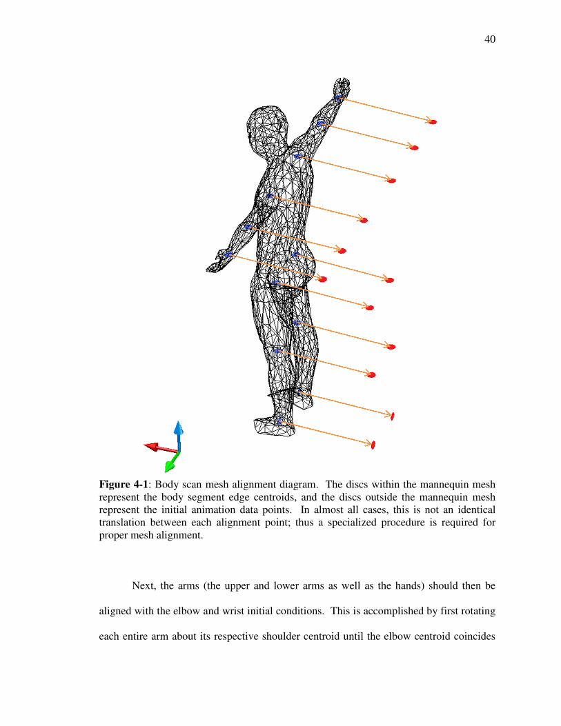
Figure 4-1: Body scan mesh
represent the body segment edge centroids, and the discs outs
represent the initial animation data points. In almost all cases, this is not an identical
translation between each alignment point; thus a specialized procedure is required for
proper mesh alignment.
Next, the arms (the upper an
aligned with the elbow and wrist initial conditions. This is accomplished by first rotating
each entire arm about its respective shoulder centroid until the elbow centroid coincides
ody scan mesh alignment diagram. The discs within the mannequin mesh
represent the body segment edge centroids, and the discs outside the mannequin mesh
represent the initial animation data points. In almost all cases, this is not an identical
translation between each alignment point; thus a specialized procedure is required for
Next, the arms (the upper and lower arms as well as the hands) should then be
aligned with the elbow and wrist initial conditions. This is accomplished by first rotating
each entire arm about its respective shoulder centroid until the elbow centroid coincides
40
The discs within the mannequin mesh
ide the mannequin mesh
represent the initial animation data points. In almost all cases, this is not an identical
translation between each alignment point; thus a specialized procedure is required for
d lower arms as well as the hands) should then be
aligned with the elbow and wrist initial conditions. This is accomplished by first rotating
each entire arm about its respective shoulder centroid until the elbow centroid coincides
41
with the initial elbow data point. The lower arm and hand are then rotated about the
elbow centroids until the wrist centroids coincide with the initial wrist data points. This
is very similar to the step used to place the mannequin mesh into the neutral posture prior
to shoulder reconstruction, but on a finer scale. Because the body scan was obtained such
that the global axes are aligned with major body features as discussed in Chapter 3 and in
a posture consistent with the neutral posture, the body segments do not need to be rotated
about an internal axis. That is to say, the orientation of each body segment with respect
to the mannequin mesh as a whole is correct in the form contained in the body scan; only
the body segment edges need to be relocated to match the data. Hence, any portion of the
mannequin that is facing the frontal direction, for example, will still be facing the frontal
direction of the mannequin post-alignment. This is true for all body segments.
In addition, note that the mannequin as a whole may be reoriented to match the
animation data axes definitions, but a body segment will not change direction with
respect to another body segment except for slight changes due to slight discrepancies
between the body scan posture and the neutral posture.
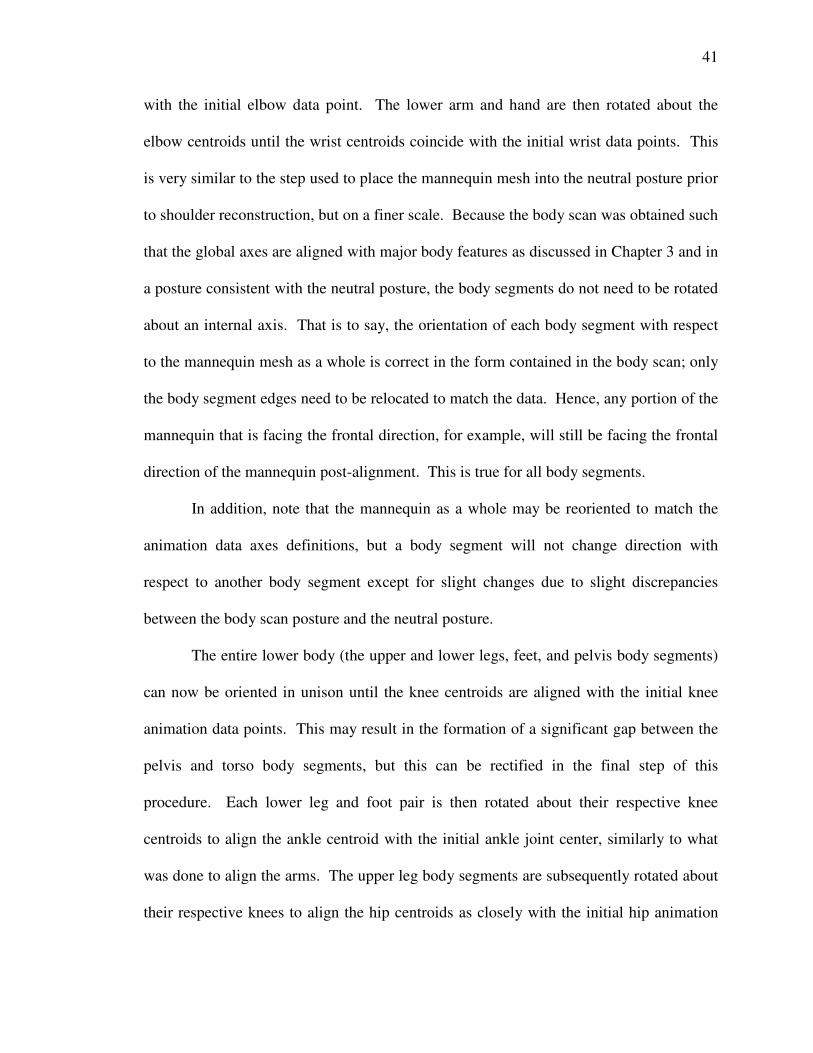
The entire lower body (the upper and lower legs, feet, and pelvis body segments)
can now be oriented in unison until the knee centroids are aligned with the initial knee
animation data points. This may result in the formation of a significant gap between the
pelvis and torso body segments, but this can be rectified in the final step of this
procedure. Each lower leg and foot pair is then rotated about their respective knee
centroids to align the ankle centroid with the initial ankle joint center, similarly to what
was done to align the arms. The upper leg body segments are subsequently rotated about
their respective knees to align the hip centroids as closely with the initial hip animation
42
data points. Because of the unique segmentation at the hips, the hip centroids may not
correspond directly with the complementary initial conditions of the hips from the
animation data (see Fig. 4-2).
Figure 4-2: Hip alignment discrepancy. The image on the left is of a perspective view
showing the vertical difference, and the image on the right is viewed from the top of the
mannequin showing that the points are nearly coplanar after alignment is completed. The
body segment edge centroids are depicted by the set of darker rings and segments, and
the data from the first time step is depicted by white rings and segments.
The vertical coordinate of the centroids and the initial conditions at the hip should
be relatively close (though not exact), as should the frontal coordinates, whereas the
lateral coordinates of the centroids will be closer to the median plane than their initial
condition counterparts. When properly aligned, the hip centroids will be as close as
possible to lying within the same coronal plane as the hip initial conditions. As is the
case with the images captured in Fig. 4-2, discrepancies between the motion capture data
and the body scan mean that perfect alignment may not be possible.

The final step is to rotate the torso and head, in tandem, about a line segment
between the two shoulder
edges meet as closely as possible (see Fig. 4
the pelvis-torso and neck body segment edges will not correspond with their initial
condition counterparts. With this final step complete, the mannequin is ready to be
animated with the data to which it was aligned.
Figure 4-3: Image of the final mesh alignment step. The axis of rotation is depicted by
the solid line connecting (and extending beyond) t
The neck and pelvis-torso body segment edge centroids are the only centroids not aligned
with their initial condition counterparts.
Although not necessary
manipulated to match for visual continuity of the mannequin mesh
unless the animation data
are always identical, the procedure described above must be performed for each new da
The final step is to rotate the torso and head, in tandem, about a line segment
shoulder edge centroids until the shared torso and pelvis
edges meet as closely as possible (see Fig. 4-3). It is noted again that the centroids for
torso and neck body segment edges will not correspond with their initial
ts. With this final step complete, the mannequin is ready to be
animated with the data to which it was aligned.
: Image of the final mesh alignment step. The axis of rotation is depicted by
the solid line connecting (and extending beyond) the two shoulder body segment edges.
torso body segment edge centroids are the only centroids not aligned
with their initial condition counterparts.
Although not necessary, the mesh polygons at adjacent body segments can be
for visual continuity of the mannequin mesh. It is
unless the animation data control points can be obtained such that the initial conditions
are always identical, the procedure described above must be performed for each new da
43
The final step is to rotate the torso and head, in tandem, about a line segment
torso and pelvis body segment
3). It is noted again that the centroids for
torso and neck body segment edges will not correspond with their initial
ts. With this final step complete, the mannequin is ready to be
: Image of the final mesh alignment step. The axis of rotation is depicted by
he two shoulder body segment edges.
torso body segment edge centroids are the only centroids not aligned
the mesh polygons at adjacent body segments can be
is also noted that
control points can be obtained such that the initial conditions
are always identical, the procedure described above must be performed for each new data

44
set. The need for a standard initial posture is most pressing when the data for animation
the mannequin is obtained through motion capture. When animating the mannequin with
predicted joint angle time histories, the actual location of the joint centers will depend
upon the mannequin anthropometry, which can be obtained from the body segment
meshes.
4.2 Mannequin Animation with Motion Capture Data
A major goal of this thesis is to develop a methodology for animating the
mannequin with motion capture data from various sources. To do this efficiently, the
methodology developed relies on local coordinate systems to update the special location
and orientation of a given body segment mesh at a given instant in time from only the
simultaneous position vectors of three animation data points, or control points.
Incidentally, motion capture data should be collected so that there are a minimum of three
non-collinear control points for each body segment.
The three control points are utilized at each time step to determine the local
coordinate system position and orientation within a global coordinate reference
framework. Two of the control points are located on either end of the body segment at
the body segment edge centroids, with the third control point between the first two, but
offset, to capture rotation (see Fig. 4-4). The body segment edge centroids represent
easy-to-obtain locations that also correspond roughly with human body joint centers,
making them ideal choices with which to develop the body segment local coordinate
system.

Figure 4-4: Body segment control point diagram. Given the location of 3 points on each
body segment, and assuming rigid body motion, the location and orientation of each body
segment local coordinate system
segment edge locations in global coordinates can be calculated.
With shared body segment edge
at the elbow can be used to animate both the upper and lower
independent body segments,
This is no more than would be required to animate the same number of body segments
were they modeled by spheres and ellipsoids
The animation procedur
segment mesh node in terms of its
accomplished by first obtaining
����, ���, ���� for each body segment
longitudinal axis defines the position vector of the local coordinate system origin
calculated utilizing Equations 4.2 and 4.3.
longitudinal vector ���� −
: Body segment control point diagram. Given the location of 3 points on each
body segment, and assuming rigid body motion, the location and orientation of each body
local coordinate system can be determined. From this information, the body
segment edge locations in global coordinates can be calculated.
body segment edges yielding only one control point (
at the elbow can be used to animate both the upper and lower arms), and a total of 10
independent body segments, at most 24 points are needed to animate the mannequin.
This is no more than would be required to animate the same number of body segments
were they modeled by spheres and ellipsoids!
The animation procedure first requires establishing the coordinates of each body
terms of its own segment-specific local coordinate system
first obtaining the three initial condition control point
each body segment. The projection of the third control point onto the
longitudinal axis defines the position vector of the local coordinate system origin
calculated utilizing Equations 4.2 and 4.3. The first basis vector �̃� is parallel to the
� � − ���� and is calculated employing Eq. 4.4.
45
: Body segment control point diagram. Given the location of 3 points on each
body segment, and assuming rigid body motion, the location and orientation of each body
From this information, the body
one control point (e.g. the centroid
s), and a total of 10
24 points are needed to animate the mannequin.
This is no more than would be required to animate the same number of body segments
establishing the coordinates of each body
local coordinate system. This is
initial condition control point position vectors
The projection of the third control point onto the
longitudinal axis defines the position vector of the local coordinate system origin ���,
is parallel to the
and is calculated employing Eq. 4.4. By Eq. 4.5, the
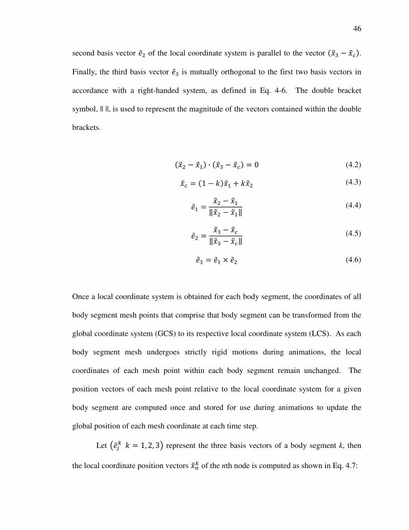
46
second basis vector �̃� of the local coordinate system is parallel to the vector ���� − ����.
Finally, the third basis vector �̃� is mutually orthogonal to the first two basis vectors in
accordance with a right-handed system, as defined in Eq. 4-6. The double bracket
symbol, || ||, is used to represent the magnitude of the vectors contained within the double
brackets.
���� − ���� ∙ ���� − ���� = 0 ��� = �1 − ����� + ���� �̃� = ��� − ������� − ����
�̃� = ��� − ������� − ����
�̃� = �̃� × �̃�
Once a local coordinate system is obtained for each body segment, the coordinates of all
body segment mesh points that comprise that body segment can be transformed from the
global coordinate system (GCS) to its respective local coordinate system (LCS). As each
body segment mesh undergoes strictly rigid motions during animations, the local
coordinates of each mesh point within each body segment remain unchanged. The
position vectors of each mesh point relative to the local coordinate system for a given
body segment are computed once and stored for use during animations to update the
global position of each mesh coordinate at each time step.
Let �̃!" � = 1, 2, 3% represent the three basis vectors of a body segment k, then
the local coordinate position vectors ��&" of the nth node is computed as shown in Eq. 4.7:
(4.2)
(4.3)
(4.4)
(4.6)
(4.5)

47
��&" = '(" ∙ )(&" − ���"% ∈ +1, 2, ⋯ , -".
where )(&" is the position vector of the nth node of the kth segment in a global coordinate
system, ���" is the position vector of the kth segment’s local coordinate system origin
within the global coordinate system, and '(" is a 3x3 orthogonal transformation matrix in
which the basis vectors �̃!" � = 1, 2, 3% are arranged such that �̃�" encompasses the first
row, �̃�" the second, and �̃�" the third. The location of each body segment mesh point in
terms of its local coordinates is used to compute the updated location of the same point in
the global coordinate system. That is, at a given time t of an animation assume that we
are given the global coordinates of the three control points for the kth body segment
����", ���" , ���"�. The instantaneous local basis vectors �̃!" � = 1, 2, 3% and the
instantaneous LCS origin ���" of the local basis relative to the global origin can be
computed directly using Equations 4.2 through 4.6. Then, the global coordinates of each
node that comprises the kth body segment is computed by inverting Eq. 4.7 into the form
shown in Eq. 4.8, through which the instantaneous global position vector of the nth node
of the kth body segment is computed.
)(&" = ���" + '("%/ ∙ ��&" ∈ +1, 2, ⋯ , -".
With a body scan mesh prepared as discussed in Chapter 3 and properly aligned
with a set of animation data as presented earlier in this chapter, the mannequin can be
made to perform any task that can be taken motion capture data (see Fig. 4-5).
(4.8)
(4.7)

48
Figure 4-5: Mannequin animated with motion capture data. The subject is seen at
various points throughout a “stretching” routine.
4.3 Mannequin Animation with Joint Angle Histories
The Virtual Soldier Research group at the University of Iowa uses DH (Denavit-
Hartenberg) kinematics to model the human body skeleton, which is represented visually
with an avatar named Santos™. Utilizing DH kinematics allows for any given posture to
be determined by a set of variables for each degree of freedom, attached via rigid
connections, called links, forming a kinematic chain.
The overall effect of a group of linked joints – the kinematic chain - is the
propagation of motion from the summation of the individual effects of each degree of
freedom. This is analogous to multi-segmented machinery, such as a robotic arm, where
the summation of each of the individual joint motions results in the final location of the

end of the robotic arm. (The end location of a kinematic chain is henceforth referred to
as the end effecter.) A simple example of a two
in Fig. 4-6.
Figure 4-6: Two-dimensional representation of a kinematic chain. The motion of each
link in the chain contributes to the final location of the end effecter, and each
contribution to the final location can be represented mathematically by a series of
transformation matrices.
In Configuration A of Fig. 4
defined in the image. If the origin is located at
global coordinates is then
Configuration B shows the kinematic chain after a separate rigid body rotation is applied
to each joint. The variables
freedom. A positive rotation is
end of the robotic arm. (The end location of a kinematic chain is henceforth referred to
.) A simple example of a two-dimensional kinematic chain is provided
dimensional representation of a kinematic chain. The motion of each
link in the chain contributes to the final location of the end effecter, and each
contribution to the final location can be represented mathematically by a series of
In Configuration A of Fig. 4-6, the three links are perfectly flat along the x
defined in the image. If the origin is located at (0, 0), the location of the end effecter
then ��� + �� + ��, 0�, where L1, L2, and L3 are the link lengths
Configuration B shows the kinematic chain after a separate rigid body rotation is applied
to each joint. The variables q1, q2, and q3 are the joint angles applied to each degree of
A positive rotation is defined as counter-clockwise.
49
end of the robotic arm. (The end location of a kinematic chain is henceforth referred to
dimensional kinematic chain is provided
dimensional representation of a kinematic chain. The motion of each
link in the chain contributes to the final location of the end effecter, and each link
contribution to the final location can be represented mathematically by a series of
6, the three links are perfectly flat along the x-axis
the location of the end effecter in
are the link lengths.
Configuration B shows the kinematic chain after a separate rigid body rotation is applied
are the joint angles applied to each degree of

50
The individual effect of each of the links on the end effecter location is apparent
by examination of Configuration B. Indeed, the location of the end effecter can be
determined through the cumulative effects of all links in the kinematic chain. To
accomplish this, a structured system is required for determining the local coordinate
system of each joint so that the end effecter location can be transformed through each
reference frame until it is expressed in terms of the global coordinate system. To this
end, the local coordinate system x-axis for joint i is defined in the direction of joint i to
joint i+1, and the z-axis (the axis of rotation) is defined using a right-handed coordinate
system; in Fig. 4-6 and the proceeding two-dimensional examples, a positive rotation is
defined as counter-clockwise, thus the local coordinate z-axis for each joint is pointing
out of the page. The y-axis is defined as the cross-product of the z- and x-axes. By
convention, the local coordinate system origin is placed at the distal end of the link, so
the local coordinate system origin for joint 0 is located at joint 1 on link 0, and so on.
Moreover, link i and joint i have the same local coordinate system.
With these conventions in place, it can be shown that a transformation matrix for
each degree of freedom (joint) can be developed to convert a point (end effecter) from
one reference frame to the next. The transformation matrix for such a two-dimensional
link is written as follows [15]:
012� 1 = 3cos 71 − sin 71 :1 cos 71sin 71 cos 71 :1 sin 710 0 1 ;
in which qi is the joint angle and ai is the link length for the current reference frame, i. In
Eq. 4.9, the joint angle value is expressed relative to the local coordinate x-axis of the
(4.9)
51
proximal joint. For example, the joint angle for joint 2 (q3) is expressed relative to the
local coordinate system x-axis of joint 1. The sub- and superscripts of 012� 1 signify that
the transformation matrix converts the coordinates from the current reference frame (i) to
that of the proximal reference frame (i-1). Using Fig. 4-6 to demonstrate by converting
the location of joint 1 into global coordinates, Eq. 4.9 is rewritten as shown in Eq. 10.
0< � = 3cos 7� − sin 7� �� cos 7�sin 7� cos 7� �� sin 7�0 0 1 ;
In Eq. 4.10, 0< � denotes that the transformation matrix converts a point from the
reference frame at joint 1 to the base reference frame at joint 0. Notice that only one
transformation matrix is required as the end effecter, joint 1, is only converted through
one reference frame. Joint 1 expressed in terms of the reference frame for link 0 is
simply (0, 0) since the local coordinate system origin is located at the distal end of the
link. Were the point to be converted located at the midpoint of link 0, the local
coordinates would be (−��/2, 0). For use with Eq. 4.10, the local coordinate system
position vector of the point to be transformed is represented in an augmented form, with
the third term in the vector is always equal to identity for a two-dimensional link:
��& = >�&?&1 @
in which ��& is the augmented local coordinate position vector of a point on link n, �& is
the local x-coordinate of the end effecter, and ?& is the local y-coordinate. With the
(4.10)
(4.11)
52
augmented local position vector of �0, 0, 1� for joint 1 in terms of the joint 0 local
coordinate system, the product of Eq. 4.10 and the augmented position vector of joint 1
will yield the global position vector for joint 1:
3cos 7� − sin 7� �� cos 7�sin 7� cos 7� �� sin 7�0 0 1 ; 3001; = 3�� cos 7��� sin 7�1 ;
This result can be quickly verified through inspection of Fig. 4-6. In the preceding
example, joint 1 was treated as the end effecter for link 0. It is important to recognize
that the end effecter need not be at the end of the entire kinematic chain defined in a DH
model. Rather, the end effecter can be placed anywhere in a kinematic chain where a
point’s location is sought. This fact means that any control point sought need only be
placed at the equivalent location of the DH model – the position at which all of the
degrees of freedom in the DH model that contribute to that control point’s ultimate
location will have an effect.
To determine the location of the end effecter shown in Fig. 4-6 using the
conventions set up for use with Eq. 4.10, a cumulative transformation matrix representing
the change in reference frame along the kinematic chain, from link 2 to the global
reference frame, is needed. The process by which the cumulative product of a series of
transformation matrices is determined is written mathematically in Eq. 4.13, while the
location of the end effecter with respect to the new reference frame is represented by Eq.
4.14 [15]. In the following equations, the position vector ���7�� is the animation control
point in global coordinates after the chain effect of all of the predecessor links
contributing to the end effecter’s ultimate location has been determined. ��&, a 3x1 matrix
(4.12)
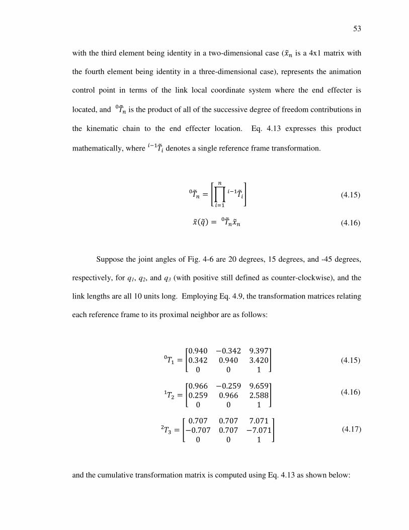
53
(4.15)
(4.16)
(4.17)
(4.15)
(4.16)
with the third element being identity in a two-dimensional case (��& is a 4x1 matrix with
the fourth element being identity in a three-dimensional case), represents the animation
control point in terms of the link local coordinate system where the end effecter is
located, and 0(&< is the product of all of the successive degree of freedom contributions in
the kinematic chain to the end effecter location. Eq. 4.13 expresses this product
mathematically, where 0(112� denotes a single reference frame transformation.
0(&< = 3A 0(112�&1B� ;
���7�� = 0(&< ��&
Suppose the joint angles of Fig. 4-6 are 20 degrees, 15 degrees, and -45 degrees,
respectively, for q1, q2, and q3 (with positive still defined as counter-clockwise), and the
link lengths are all 10 units long. Employing Eq. 4.9, the transformation matrices relating
each reference frame to its proximal neighbor are as follows:
0< � = 30.940 −0.342 9.3970.342 0.940 3.4200 0 1 ;
0� � = 30.966 −0.259 9.6590.259 0.966 2.5880 0 1 ;
0� � = 3 0.707 0.707 7.071−0.707 0.707 −7.0710 0 1 ;
and the cumulative transformation matrix is computed using Eq. 4.13 as shown below:

54
(4.18)
(4.19)
0< � 0� � 0� � = 0< � = 3 0.985 0.174 27.437−0.174 0.985 7.4190 0 1 ;
The end effecter is located at �0, 0� in the local coordinate system of joint 2, so the
position of the end effecter in terms of the global coordinate system in Fig. 4-6 is
calculated using Eq. 4.14.
���7�� = 3 0.985 0.174 27.437−0.174 0.985 7.4190 0 1 ; 3001; = 327.4377.4191 ;
in which �27.437, 7.419� is the global position vector of the end effecter. Noting that
the joint angles of 20, 15, and -45 degrees are equivalent to angles of 20, 35, and -10
degrees expressed with respect to the global coordinate system, the result in Eq. 4.19 can
be easily verified.
In three dimensions, the initial placement of each link with respect to its neighbor
is defined by four parameters (see Fig. 4-7). The parameters in Fig. 4-7 can then be
described as follows: J1 is the angle between the x-axis of joint i-1 and that of joint i,
about the axis of rotation (the z-axis) of joint i-1, K1 is the angle between the z-axis of
joint i-1 and joint i, ai is the distance from the z-axis of joint i-1 to the z-axis of joint i,
and di is the distance between the x-axes of joints i-1 and i. The joint angle variable qi
has the same definition as J1 in Fig. 4-7 because a revolute joint is depicted. Both di and
ai represent a link length as is defined in this thesis, a term used to describe the three-
dimensional distance between two successive degrees of freedom along a given global
axis. In practice, J1, K1, di, and ai are referred to the joint angle, link twist, link offset,
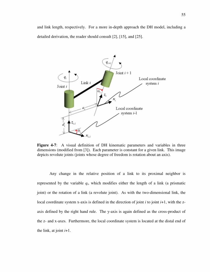
55
and link length, respectively. For a more in-depth approach the DH model, including a
detailed derivation, the reader should consult [2], [15], and [25].
Figure 4-7: A visual definition of DH kinematic parameters and variables in three
dimensions (modified from [3]). Each parameter is constant for a given link. This image
depicts revolute joints (joints whose degree of freedom is rotation about an axis).
Any change in the relative position of a link to its proximal neighbor is
represented by the variable qi, which modifies either the length of a link (a prismatic
joint) or the rotation of a link (a revolute joint). As with the two-dimensional link, the
local coordinate system x-axis is defined in the direction of joint i to joint i+1, with the z-
axis defined by the right hand rule. The y-axis is again defined as the cross-product of
the z- and x-axes. Furthermore, the local coordinate system is located at the distal end of
the link, at joint i+1.

56
Each of the parameter values is determined based upon the orientation of the local
coordinate system axes at each degree of freedom. Thus, the neutral posture is chosen
with the mannequin standing fully upright and with the arms extended fully outwards as
this represents an angle of magnitude π/2 or 180 degrees between the majority of links in
the mannequin. Knowing the orientation of each LCS in the avatar model, the two
angular parameters can be determined. The link lengths values are simply derived from
the mannequin anthropometry (i.e. the lengths of bones, etc.).
Because each degree of freedom is represented by a single DH kinematic joint, a
relationship is developed whereby the link lengths correspond to the physical lengths of
the bones in the human body that the link and degree of freedom model. This also means
that when the joints modeled are capable of more than one degree of freedom of motion,
the link lengths between the two degrees of freedom at the joint is zero. In addition to
being used as the approximate DH joint locations, the body segment edge centroids are
used to determine these link lengths; though because the mannequin used in this thesis
uses significantly fewer degrees of freedom than the DH model from which the animation
control points were obtained, approximations were used to obtain many of the link
lengths needed in the DH model from the body segment edge centroids. This process
will be described in detail later in this chapter.
The joint angle, qi, is the only unknown at each time step and is defined about the
z-axis of the proximal joint (this is the same convention as is used to define J1) for
revolute joints (joints that rotate about a single axis), and coincides with the link length di
for prismatic joints (joints that extend along an axis). Transcribing these variables into

57
(4.20)
the transformation matrix, 012� 1, relating the position of the current joint with respect to
the coordinate system of the previous joint yields Eq. 4.20 [15].
012� 1 = L cos J1 − cos K1 sin J1 sin J1 cos K1 cos J1 sin K1 sin J1 :1 cos J1 − sin K1 cos J1 :1 sin J1 0 sin K1 0 0 cos K1 M10 1 N
It is interesting to note that Eq. 4.9 can be derived from Eq. 4.20: in the two-dimensional
case, both angle variables are zero, as is the value of di. This creates all zeros in the third
row and third column of Eq. 4.20, which when removed yield Eq. 4.9!
A DH kinematics-driven skeletal model consists of several smaller kinematic
chains (see Fig. 4-8). The pelvis is considered the base from which the kinematic chains
emanate; however, to represent the motion of the model as a whole with respect to the
global inertial frame, six degrees of freedom are modeled as a kinematic chain from the
global coordinate origin to the pelvis (three of these are revolute joints representing the
rotation of the DH model about the three global axes, while the other three degrees of
freedom are the only prismatic joints incorporated in the DH model and represent the
motion in terms of the global axes). From the pelvis, three parent chains – the spine, the
right leg, and the left leg – describe the motion of the torso and legs, respectively. In
addition, to represent the head and arms, three child kinematic chains also emanate from
the end of the spine kinematic chain – one for each arm and another for the neck and
head. In addition, because the local coordinate system origin for each degree of freedom
is located at the distal end of the link from the previous joint, the first degree of freedom
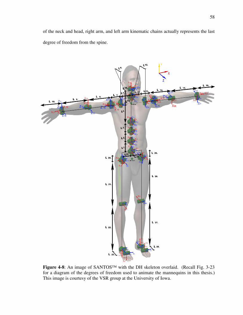
58
of the neck and head, right arm, and left arm kinematic chains actually represents the last
degree of freedom from the spine.
Figure 4-8: An image of SANTOS™ with the DH skeleton overlaid. (Recall Fig. 3-23
for a diagram of the degrees of freedom used to animate the mannequins in this thesis.)
This image is courtesy of the VSR group at the University of Iowa.
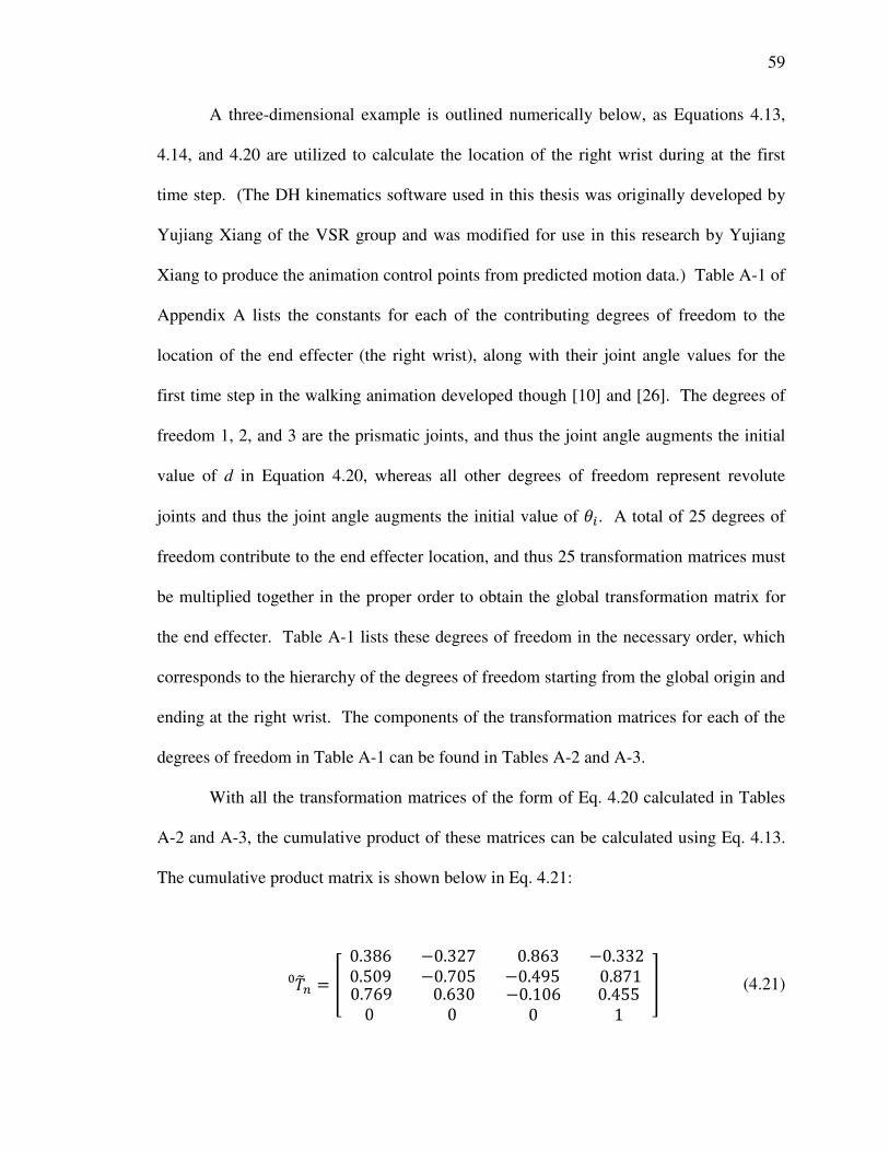
59
(4.21)
A three-dimensional example is outlined numerically below, as Equations 4.13,
4.14, and 4.20 are utilized to calculate the location of the right wrist during at the first
time step. (The DH kinematics software used in this thesis was originally developed by
Yujiang Xiang of the VSR group and was modified for use in this research by Yujiang
Xiang to produce the animation control points from predicted motion data.) Table A-1 of
Appendix A lists the constants for each of the contributing degrees of freedom to the
location of the end effecter (the right wrist), along with their joint angle values for the
first time step in the walking animation developed though [10] and [26]. The degrees of
freedom 1, 2, and 3 are the prismatic joints, and thus the joint angle augments the initial
value of d in Equation 4.20, whereas all other degrees of freedom represent revolute
joints and thus the joint angle augments the initial value of J1. A total of 25 degrees of
freedom contribute to the end effecter location, and thus 25 transformation matrices must
be multiplied together in the proper order to obtain the global transformation matrix for
the end effecter. Table A-1 lists these degrees of freedom in the necessary order, which
corresponds to the hierarchy of the degrees of freedom starting from the global origin and
ending at the right wrist. The components of the transformation matrices for each of the
degrees of freedom in Table A-1 can be found in Tables A-2 and A-3.
With all the transformation matrices of the form of Eq. 4.20 calculated in Tables
A-2 and A-3, the cumulative product of these matrices can be calculated using Eq. 4.13.
The cumulative product matrix is shown below in Eq. 4.21:
0(&< = O 0.386 −0.327 0.509 −0.705 0.863 −0.332 −0.495 0.871 0.769 0.630 0 0 −0.106 0.4550 1 P

60
(4.22)
As the end effecter is positioned, it is located at the distal end of the forearm link.
Thus, the position vector in terms of the forearm link local coordinate system, expressed
in the three-dimensional form of Eq. 4.11, is ��& = �0 0 0 1�. Eq. 4.14 is used to
determine the location of the end effecter in global coordinates:
���7�� = O 0.386 −0.327 0.509 −0.705 0.863 −0.332 −0.495 0.871 0.769 0.630 0 0 −0.106 0.4550 1 P O 0 001 P = O−0.332 0.8710.4551 P
where the global position vector of the end effecter (the right wrist) is
�−0.332, 0.871, 0.455�. These control point location calculations are done at each
time step for all 24 control points, creating the data needed to animate the mannequin
from the predicted motion in terms of the DH model. It is noted that the DH model
employed for these calculations uses a different set of global axes definitions than is
generally used in this thesis. More specifically, the DH model defines the global x-axis
as the lateral direction, the global-y axis as the vertical direction, and the global z-axis as
the frontal direction.
Utilizing predicted motion data to animate a mannequin is more convenient than
using motion capture data because each of these constants, sans the link lengths, is
mannequin model-independent, meaning they are the same for any given DH model as
long as the degrees of freedom represented by each DH model are identical. This allows
for a given predicted motion to be used to animate any mannequin as long as the link
lengths for the mannequin are known – and as mentioned earlier, with the body segment
edges known, determining the link lengths for the mannequin is trivial.

61
With the mannequin is oriented similar to Fig. 3-1, the distances between
successive body segment edge centroids will only be along a single global axis, and thus
will only correspond to either ai or di of Eq. 4.13 (depending upon how the LCS axes are
oriented as discussed earlier) except in the case of the clavicle, as it is the only link that
traverses through two dimensions in the neutral posture; however, the clavicle link
lengths are still trivial to determine. The frontal distance traversed by the clavicle is
simply the frontal distance between the shoulder and neck body segment edge centroids,
with the lateral distance between these body segment edge centroids equating to the
lateral distance traversed by the clavicle. This procedure is straight-forward for each
body segment modeled except for the torso. The torso body segment is a single link in
the mannequin model but encompasses five different joints in the DH model (four in the
torso and one in the neck). Simple ratios were applied to circumvent this issue whereby
the link lengths for the DH model were extrapolated from the single link length of the
torso. First, the link length between the clavicle and the neck was determined by taking
the vertical distance between the shoulder and neck body segment edges, and the
remaining distance was split into the four remaining joints according to their relative
dimensions in the DH model. That is to say, taking the cumulative length of the four DH
model torso links as 1 meter for simplicity, and assuming arbitrarily that the first three
links are each 15% of the cumulative length, then the corresponding link lengths of a
mannequin would be 15% of the mannequin torso vertical dimension, with the fourth link
length encompassing the remaining 55% of the torso vertical dimension. This
approximation works well to circumvent the lack of detailed information of a subject
scan when attempting to animate the subject mannequin, but its effects on any subsequent
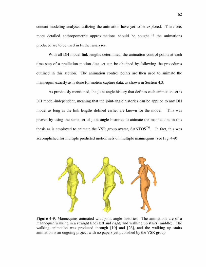
62
contact modeling analyses utilizing the animation have yet to be explored. Therefore,
more detailed anthropometric approximations should be sought if the animations
produced are to be used in further analyses.
With all DH model link lengths determined, the animation control points at each
time step of a prediction motion data set can be obtained by following the procedures
outlined in this section. The animation control points are then used to animate the
mannequin exactly as is done for motion capture data, as shown in Section 4.3.
As previously mentioned, the joint angle history that defines each animation set is
DH model-independent, meaning that the joint-angle histories can be applied to any DH
model as long as the link lengths defined earlier are known for the model. This was
proven by using the same set of joint angle histories to animate the mannequins in this
thesis as is employed to animate the VSR group avatar, SANTOSTM
. In fact, this was
accomplished for multiple predicted motion sets on multiple mannequins (see Fig. 4-9)!
Figure 4-9: Mannequins animated with joint angle histories. The animations are of a
mannequin walking in a straight line (left and right) and walking up stairs (middle). The
walking animation was produced through [10] and [26], and the walking up stairs
animation is an ongoing project with no papers yet published by the VSR group.

63
4.4 Data Formatting
The animation software written for this thesis, in order to be truly data source-
independent, required a generic data formatting system. To that end, three data file types
are used: a master file, the control file, which contains animation summary information as
well as global translation and rotations to be applied to each body segment data file; body
segment data files, which store body segment mesh connectivity information and
segment-specific translations and rotations to be performed prior to animation; and the
animation data file, wherein all of the animation time steps are contained. All of the data
contained in the files are in terms of global coordinates, and will only be converted to
body segment-specific local coordinate systems by the animation software as needed to
update the mesh at each time step.
More specifically, the control file is needed to inform the software of the number
of segments to be animated, the number of control points to be used to animate the files,
the number of animation steps in the animation data file, the sequence by which the
animation data file is read, and any translation or rotation scheme that is to be applied to
all body segment animation files (see Box 4-1).
Box 4-1: Sample animation control file.
In the sample control file provided in Box 4-1, there are 31 body segment files to
animate using 24 animation control points and an animation data file that contains 202
31 24 202 1
1.0 0.0 0.0
0.0 1.0 0.0
0.0 0.0 1.0
0.0 0.0 0.0

64
time steps, through which the software is to proceed in steps of 1, as read in the first line
of the file. The latter number is useful for analyzing large sets of data in a reasonable
timeframe. For example, the motion capture data utilized in this thesis was obtained at
very small time steps (many per second), but only a fraction of the time steps are needed
to create a visually appealing mannequin animation. A value of 10 would mean that only
every tenth time step from the animation data file will be used to animate the mannequin.
The next three lines in the control file correspond to the nine components in a 3x3
transformation matrix, and the last line contains the x-, y-, and z-direction translation
values, to apply to each body segment prior to animation.
Any information that is segment-specific is placed within the body segment data
file to which it applies. Body segment-specific data includes the three control points
needed to animate the body segment, the initial body segment mesh nodal coordinates
and connectivity data, and miscellaneous information about body segment mesh pre-
processing such as rotating the mesh to fit a new axis definition or scale (see Appendix B
for an example file). Naturally, this means that there will be at least as many body
segment data files as there are independently-animated body segments. Any animation
patches can be placed in the same file as the body segment it is meant to patch; however,
it is suggested that each patch be placed in a separate control file so as to allow the
patches to be easily updated without the need to recreate the entire body segment mesh
configuration and connectivity data. Thirty-one separate body segment data files are
used in this thesis; 15 for the body segments, 12 for spherical patches, and 4 for
ellipsoidal patches.
65
In Appendix B, the first line is a description of what the body segment represents
and is ignored by the software by default. The second line informs the animation
software that this body segment data file contains 42 nodes and is to be animated using
control points 7, 23, and 9 from the animation data file. The next three lines represent the
3x3 transformation matrix to be applied specifically to this body segment data file, and
the subsequent line contains the translation to be applied. The particular file in Appendix
B is patch segment, so the translation matrix is given as the centroid of joint it is to patch.
This is because the software written to generate the spherical and ellipsoidal patch
meshes uses the origin as the centroid for simplicity. The next set of lines is devoted to
the nodal coordinates, with each node on its own line (42 in this case). The first number
in each line is the node number designation within the body segment data file, followed
by the x-, y-, and z-coordinates of the node. A single line of information proceeds the
nodal coordinate data, containing miscellaneous information about the body segment data
file. All of the information in this line is ultimately ignored by the software except for
the third component, which represents the number of elements encompassing this body
segment (40 elements in this case). The other components of this line are used by other
software for the purposes of contact modeling, which is out of the scope of this thesis and
is therefore not discussed. The final set of lines is devoted to the connectivity data. The
first constituent in each line is the element number, followed by the material type
(another piece of information only used by the contact modeling software), and the four
nodes that make up the element in order of connectivity. These node numbers
correspond directly with the nodes listed previously in the file. The animation software

66
was written to be compatible with both 3- and 4-sided elements, so 3-sided elements are
handled by giving them identical third and fourth nodes.
As mentioned earlier, a number of body segments are further divided into separate
files to create the body segment edges necessary to obtain the joint center equivalents,
from which the link lengths can be computed. These include the hands, feet, and head.
Although these portions of the mannequin are segmented, they are animated in tandem
with their adjacent body segments to limit the animation complexity.
The animation data file is simply a listing of the coordinates of each control point
at each time step, with each time step contained on a single line and the control points
listed in succession with their respective x-, y-, and z-coordinates. Following the
previous example presented in Box 4-1, the 24 control points would require that each line
have 72 entries (3 for each control point), listed as follows: control point 1 x-coordinate,
control point 1 y-coordinate, control point 1 z-coordinate, control point 2 x-coordinate,
control point 2 y-coordinate, control point 2 z-coordinate, and so on.
With the data structure just presented, the reader will have all of the information
necessary to create a realistic animation of a segmented body scan mesh from multiple
data sources, of which motion capture data and predicted motion based on a DH
kinematics-driven model were explored. As a goal of this thesis is to develop an
effective methodology for a variety of purposes, one of which was clothing contact
modeling, the next chapter will discuss the results of the use of the procedures and
methodologies presented herein as well as provide a summary to the reader.
67
CHAPTER 5
CONCLUSION
5.1 Summary
In this thesis, a framework for efficiently and effectively preparing a visually-
accurate body scan for animation was presented. It was shown that a laser scan body
mesh, once coarsened, can be segmented for the purposes of animation. An effective
segmentation pattern developed for this research was laid out with a step-by-step
procedure, allowing any body scan to be utilized as a mannequin. In addition, an
effective algorithm was presented for repairing and reconstructing portions of the body
scan mesh that were either missed by the laser scan or were created when manipulating
the mannequin into the neutral posture. A robust approach was also presented to patch
animation gaps that develop due to the use of rigid body motion assumptions in the
animation algorithm and motion capture inaccuracies, and an outline was presented for
automating the process of centroid location for the purpose of sizing the animation gap
patch geometries and determining the link lengths for use with DH-driven motion
prediction.
An efficient mannequin animation algorithm was also presented that allows for
virtually any animation data source to be used to animate the mannequin. Furthermore, a
mathematical framework was laid out for converting DH kinematics data into the
simplified format presented herein for animation of the mannequin, which opens up the
possibility for a single animation set of joint angle histories to be applied to an infinite
number of mannequins for animation. This procedure was verified with a numerical
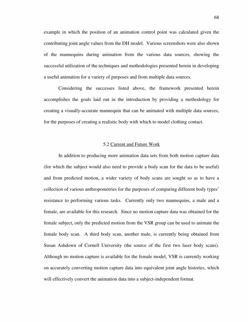
68
example in which the position of an animation control point was calculated given the
contributing joint angle values from the DH model. Various screenshots were also shown
of the mannequins during animation from the various data sources, showing the
successful utilization of the techniques and methodologies presented herein in developing
a useful animation for a variety of purposes and from multiple data sources.
Considering the successes listed above, the framework presented herein
accomplishes the goals laid out in the introduction by providing a methodology for
creating a visually-accurate mannequin that can be animated with multiple data sources,
for the purposes of creating a realistic body with which to model clothing contact.
5.2 Current and Future Work
In addition to producing more animation data sets from both motion capture data
(for which the subject would also need to provide a body scan for the data to be useful)
and from predicted motion, a wider variety of body scans are sought so as to have a
collection of various anthropometries for the purposes of comparing different body types’
resistance to performing various tasks. Currently only two mannequins, a male and a
female, are available for this research. Since no motion capture data was obtained for the
female subject, only the predicted motion from the VSR group can be used to animate the
female body scan. A third body scan, another male, is currently being obtained from
Susan Ashdown of Cornell University (the source of the first two laser body scans).
Although no motion capture is available for the female model, VSR is currently working
on accurately converting motion capture data into equivalent joint angle histories, which
will effectively convert the animation data into a subject-independent format.

69
With the animated mannequins and procedures outlined above, the follow-up to
this research is to utilize the contact algorithm of [11] and [13] to perform a complete
mannequin-clothing interaction simulation. Preliminary work has been completed in this
area; the stretching animation presented in Fig. 4-5 has been successfully used in an
animation modeling the interaction of “baggy” clothing with a mannequin (see Figures 5-
1 through 5-3). A database of animations and clothing contact-modeling analyses can be
found online at http://www.engineering.uiowa.edu/~swan/clothing/clothing.html. In
Figures 5-1 through 5-3, the mannequin is beginning to twist the upper body counter-
clockwise with respect to the first person view of the mannequin. The inertial response
of the clothing can clearly be seen in Fig. 5-1 where the clothing is pressed against the
front of the right arm and the back of the left arm, which are the leading surfaces of the
counter-clockwise twisting motion. Very little motion is occurring in the legs during this
portion of the animation, and comparison Figures 5-1 and 5-3 reveals that there is no
noticeable difference in the pants mesh, attesting to this fact.
Figure 5-1: Perspective view of the mannequin during a clothing interaction simulation.
This image was captured at 1.341 seconds into the stretching animation from Fig. 4-5.
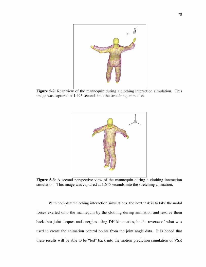
70
Figure 5-2: Rear view of the mannequin during a clothing interaction simulation. This
image was captured at 1.493 seconds into the stretching animation.
Figure 5-3: A second perspective view of the mannequin during a clothing interaction
simulation. This image was captured at 1.645 seconds into the stretching animation.
With completed clothing interaction simulations, the next task is to take the nodal
forces exerted onto the mannequin by the clothing during animation and resolve them
back into joint torques and energies using DH kinematics, but in reverse of what was
used to create the animation control points from the joint angle data. It is hoped that
these results will be able to be “fed” back into the motion prediction simulation of VSR

71
as input, causing the optimization process to change the predicted motion, in effect
creating a closed-loop system of predicted motion optimization (see Fig. 5-4).
Figure 5-4: A visual depiction of the closed-loop optimization system for motion
prediction.
Although the first completed clothing interaction simulations are just recently
being completed with the animations provided through this research, the results already
look promising. Indeed, the framework presented in this thesis for body scan preparation
and animation has allowed for an unprecedented level of accuracy in clothing simulations
and will provide a robust platform in support of future research for many years to come.
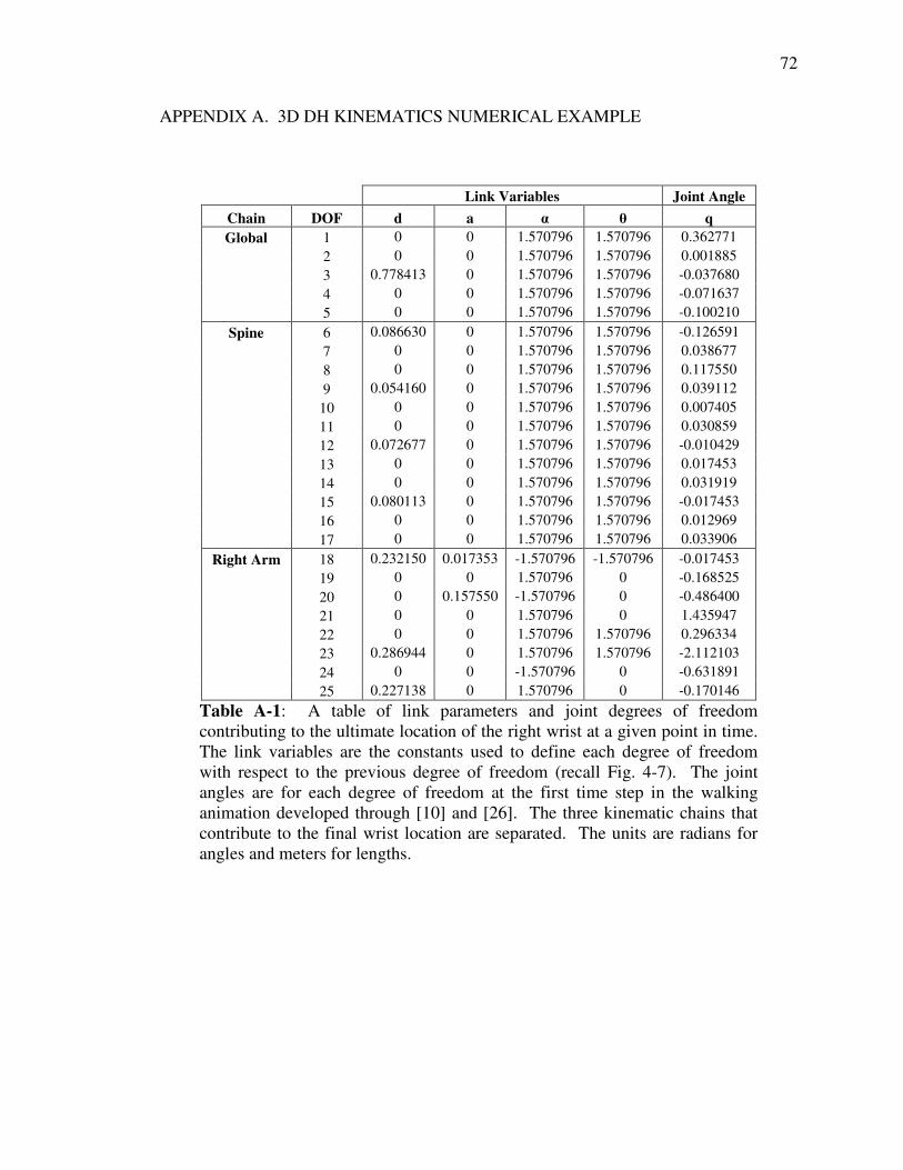
72
APPENDIX A. 3D DH KINEMATICS NUMERICAL EXAMPLE
Link Variables Joint Angle
Chain DOF d a α θ q
Global 1 0 0 1.570796 1.570796 0.362771
2 0 0 1.570796 1.570796 0.001885
3 0.778413 0 1.570796 1.570796 -0.037680
4 0 0 1.570796 1.570796 -0.071637
5 0 0 1.570796 1.570796 -0.100210
Spine 6 0.086630 0 1.570796 1.570796 -0.126591
7 0 0 1.570796 1.570796 0.038677
8 0 0 1.570796 1.570796 0.117550
9 0.054160 0 1.570796 1.570796 0.039112
10 0 0 1.570796 1.570796 0.007405
11 0 0 1.570796 1.570796 0.030859
12 0.072677 0 1.570796 1.570796 -0.010429
13 0 0 1.570796 1.570796 0.017453
14 0 0 1.570796 1.570796 0.031919
15 0.080113 0 1.570796 1.570796 -0.017453
16 0 0 1.570796 1.570796 0.012969
17 0 0 1.570796 1.570796 0.033906
Right Arm 18 0.232150 0.017353 -1.570796 -1.570796 -0.017453
19 0 0 1.570796 0 -0.168525
20 0 0.157550 -1.570796 0 -0.486400
21 0 0 1.570796 0 1.435947
22 0 0 1.570796 1.570796 0.296334
23 0.286944 0 1.570796 1.570796 -2.112103
24 0 0 -1.570796 0 -0.631891
25 0.227138 0 1.570796 0 -0.170146
Table A-1: A table of link parameters and joint degrees of freedom
contributing to the ultimate location of the right wrist at a given point in time.
The link variables are the constants used to define each degree of freedom
with respect to the previous degree of freedom (recall Fig. 4-7). The joint
angles are for each degree of freedom at the first time step in the walking
animation developed through [10] and [26]. The three kinematic chains that
contribute to the final wrist location are separated. The units are radians for
angles and meters for lengths.

73
Link Transformation Matrix Components
Chain DOF [1,1] [1,2] [1,3] [1,4] [2,1] [2,2] [2,3] [2,4]
Global 1 0.000 0.000 1.000 0.000 1.000 0.000 0.000 0.000
2 0.000 0.000 1.000 0.000 1.000 0.000 0.000 0.000
3 0.000 0.000 1.000 0.000 1.000 0.000 0.000 0.000
4 0.072 0.000 0.997 0.000 0.997 0.000 -0.072 0.000
5 0.100 0.000 0.995 0.000 0.995 0.000 -0.100 0.000
Spine 6 0.126 0.000 0.992 0.000 0.992 0.000 -0.126 0.000
7 -0.039 0.000 0.999 0.000 0.999 0.000 0.039 0.000
8 -0.117 0.000 0.993 0.000 0.993 0.000 0.117 0.000
9 -0.039 0.000 0.999 0.000 0.999 0.000 0.039 0.000
10 -0.007 0.000 1.000 0.000 1.000 0.000 0.007 0.000
11 -0.031 0.000 1.000 0.000 1.000 0.000 0.031 0.000
12 0.010 0.000 1.000 0.000 1.000 0.000 -0.010 0.000
13 -0.017 0.000 1.000 0.000 1.000 0.000 0.017 0.000
14 -0.032 0.000 0.999 0.000 0.999 0.000 0.032 0.000
15 0.017 0.000 1.000 0.000 1.000 0.000 -0.017 0.000
16 -0.013 0.000 1.000 0.000 1.000 0.000 0.013 0.000
17 -0.034 0.000 0.999 0.000 0.999 0.000 0.034 0.000
Right Arm 18 -0.017 0.000 1.000 0.000 -1.000 0.000 -0.017 -0.017
19 0.986 0.000 -0.168 0.000 -0.168 0.000 -0.986 0.000
20 0.884 0.000 0.467 0.139 -0.467 0.000 0.884 -0.074
21 0.134 0.000 0.991 0.000 0.991 0.000 -0.134 0.000
22 -0.292 0.000 0.956 0.000 0.956 0.000 0.292 0.000
23 0.857 0.000 -0.515 0.000 -0.515 0.000 -0.857 0.000
24 0.807 0.000 0.591 0.000 -0.591 0.000 0.807 0.000
25 0.986 0.000 -0.169 0.000 -0.169 0.000 -0.986 0.000
Table A-2: The first eight transformation matrix components for each degree of
freedom from Table A-1.
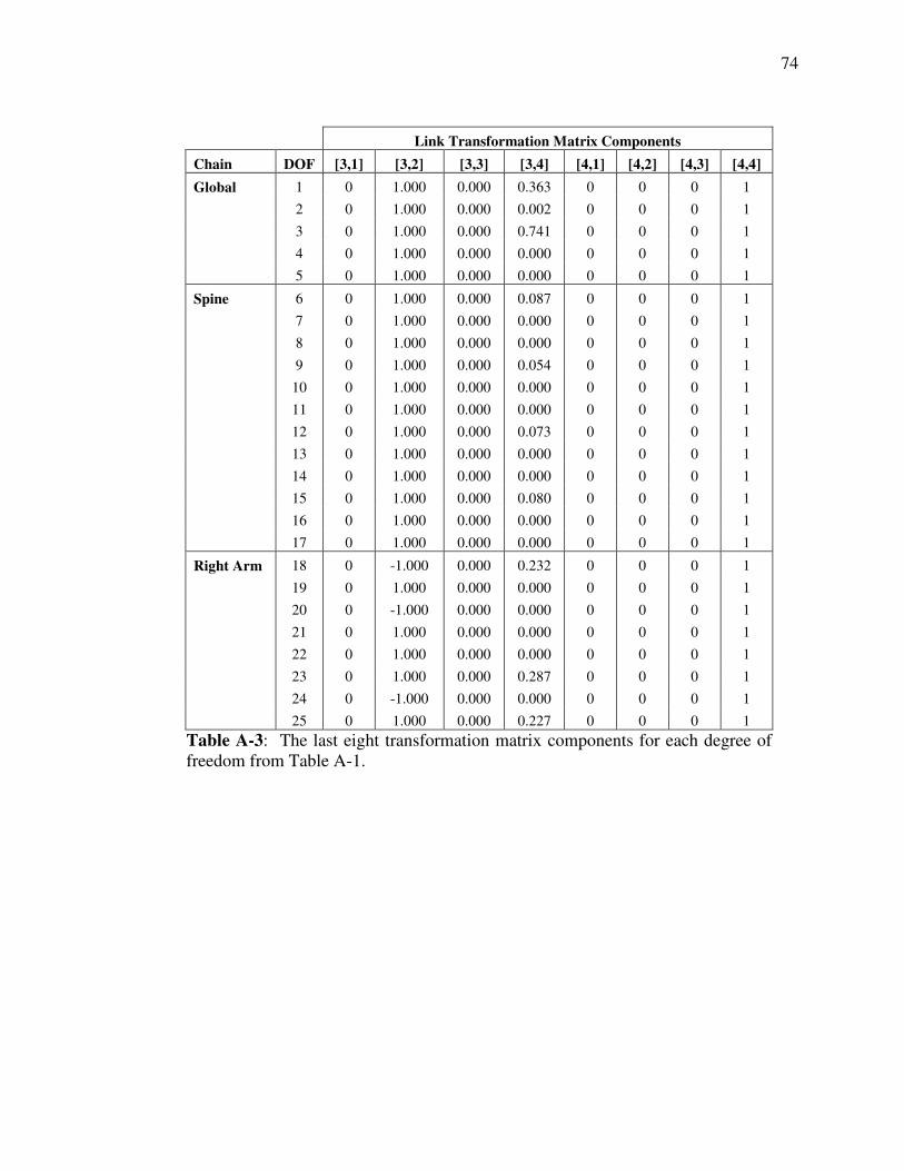
74
Link Transformation Matrix Components
Chain DOF [3,1] [3,2] [3,3] [3,4] [4,1] [4,2] [4,3] [4,4]
Global 1 0 1.000 0.000 0.363 0 0 0 1
2 0 1.000 0.000 0.002 0 0 0 1
3 0 1.000 0.000 0.741 0 0 0 1
4 0 1.000 0.000 0.000 0 0 0 1
5 0 1.000 0.000 0.000 0 0 0 1
Spine 6 0 1.000 0.000 0.087 0 0 0 1
7 0 1.000 0.000 0.000 0 0 0 1
8 0 1.000 0.000 0.000 0 0 0 1
9 0 1.000 0.000 0.054 0 0 0 1
10 0 1.000 0.000 0.000 0 0 0 1
11 0 1.000 0.000 0.000 0 0 0 1
12 0 1.000 0.000 0.073 0 0 0 1
13 0 1.000 0.000 0.000 0 0 0 1
14 0 1.000 0.000 0.000 0 0 0 1
15 0 1.000 0.000 0.080 0 0 0 1
16 0 1.000 0.000 0.000 0 0 0 1
17 0 1.000 0.000 0.000 0 0 0 1
Right Arm 18 0 -1.000 0.000 0.232 0 0 0 1
19 0 1.000 0.000 0.000 0 0 0 1
20 0 -1.000 0.000 0.000 0 0 0 1
21 0 1.000 0.000 0.000 0 0 0 1
22 0 1.000 0.000 0.000 0 0 0 1
23 0 1.000 0.000 0.287 0 0 0 1
24 0 -1.000 0.000 0.000 0 0 0 1
25 0 1.000 0.000 0.227 0 0 0 1
Table A-3: The last eight transformation matrix components for each degree of
freedom from Table A-1.
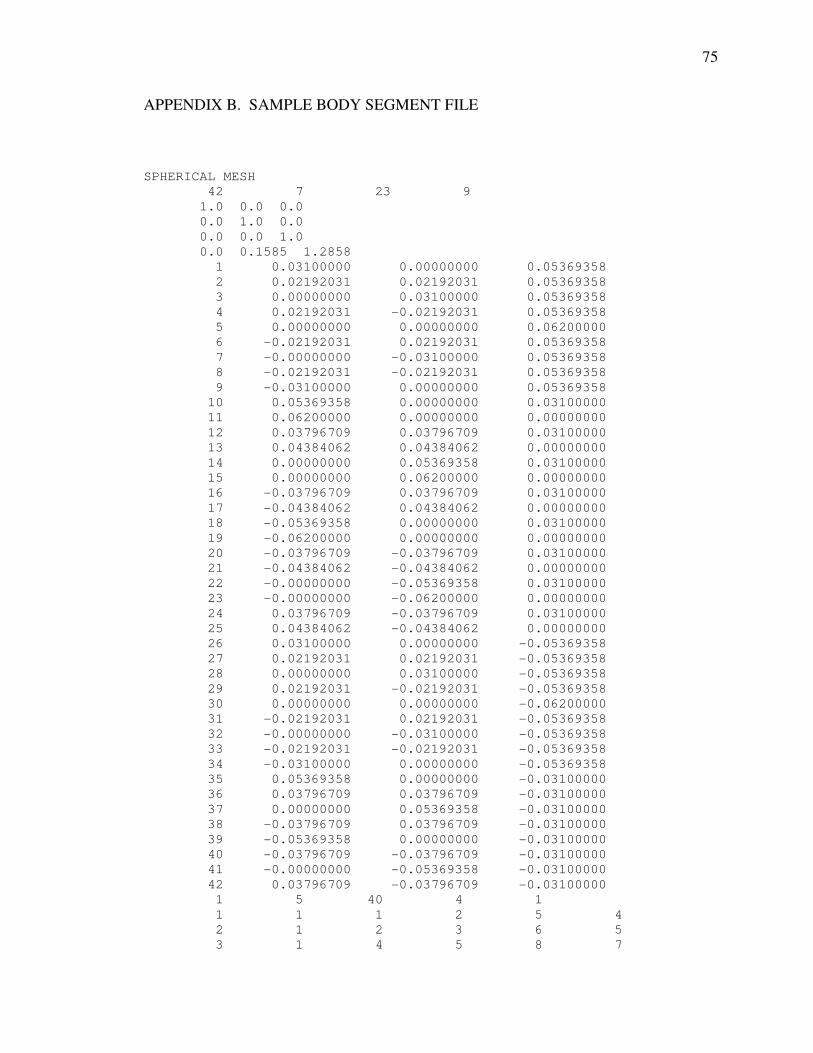
75
APPENDIX B. SAMPLE BODY SEGMENT FILE
SPHERICAL MESH
42 7 23 9
1.0 0.0 0.0
0.0 1.0 0.0
0.0 0.0 1.0
0.0 0.1585 1.2858
1 0.03100000 0.00000000 0.05369358
2 0.02192031 0.02192031 0.05369358
3 0.00000000 0.03100000 0.05369358
4 0.02192031 -0.02192031 0.05369358
5 0.00000000 0.00000000 0.06200000
6 -0.02192031 0.02192031 0.05369358
7 -0.00000000 -0.03100000 0.05369358
8 -0.02192031 -0.02192031 0.05369358
9 -0.03100000 0.00000000 0.05369358
10 0.05369358 0.00000000 0.03100000
11 0.06200000 0.00000000 0.00000000
12 0.03796709 0.03796709 0.03100000
13 0.04384062 0.04384062 0.00000000
14 0.00000000 0.05369358 0.03100000
15 0.00000000 0.06200000 0.00000000
16 -0.03796709 0.03796709 0.03100000
17 -0.04384062 0.04384062 0.00000000
18 -0.05369358 0.00000000 0.03100000
19 -0.06200000 0.00000000 0.00000000
20 -0.03796709 -0.03796709 0.03100000
21 -0.04384062 -0.04384062 0.00000000
22 -0.00000000 -0.05369358 0.03100000
23 -0.00000000 -0.06200000 0.00000000
24 0.03796709 -0.03796709 0.03100000
25 0.04384062 -0.04384062 0.00000000
26 0.03100000 0.00000000 -0.05369358
27 0.02192031 0.02192031 -0.05369358
28 0.00000000 0.03100000 -0.05369358
29 0.02192031 -0.02192031 -0.05369358
30 0.00000000 0.00000000 -0.06200000
31 -0.02192031 0.02192031 -0.05369358
32 -0.00000000 -0.03100000 -0.05369358
33 -0.02192031 -0.02192031 -0.05369358
34 -0.03100000 0.00000000 -0.05369358
35 0.05369358 0.00000000 -0.03100000
36 0.03796709 0.03796709 -0.03100000
37 0.00000000 0.05369358 -0.03100000
38 -0.03796709 0.03796709 -0.03100000
39 -0.05369358 0.00000000 -0.03100000
40 -0.03796709 -0.03796709 -0.03100000
41 -0.00000000 -0.05369358 -0.03100000
42 0.03796709 -0.03796709 -0.03100000
1 5 40 4 1
1 1 1 2 5 4
2 1 2 3 6 5
3 1 4 5 8 7
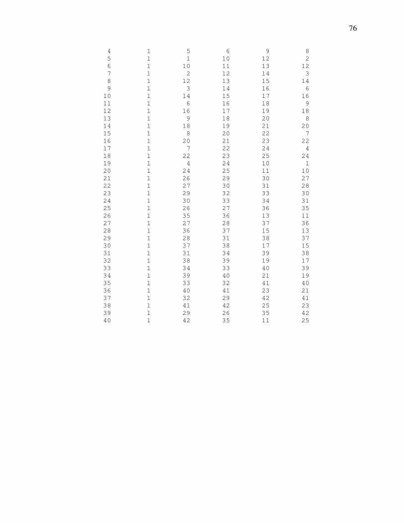
76
4 1 5 6 9 8
5 1 1 10 12 2
6 1 10 11 13 12
7 1 2 12 14 3
8 1 12 13 15 14
9 1 3 14 16 6
10 1 14 15 17 16
11 1 6 16 18 9
12 1 16 17 19 18
13 1 9 18 20 8
14 1 18 19 21 20
15 1 8 20 22 7
16 1 20 21 23 22
17 1 7 22 24 4
18 1 22 23 25 24
19 1 4 24 10 1
20 1 24 25 11 10
21 1 26 29 30 27
22 1 27 30 31 28
23 1 29 32 33 30
24 1 30 33 34 31
25 1 26 27 36 35
26 1 35 36 13 11
27 1 27 28 37 36
28 1 36 37 15 13
29 1 28 31 38 37
30 1 37 38 17 15
31 1 31 34 39 38
32 1 38 39 19 17
33 1 34 33 40 39
34 1 39 40 21 19
35 1 33 32 41 40
36 1 40 41 23 21
37 1 32 29 42 41
38 1 41 42 25 23
39 1 29 26 35 42
40 1 42 35 11 25

77
APPENDIX C. BODY SEGMENT EDGE CENTROID RESOLVER
// This program determines the edges and edge centroids of a supplied mesh
// Outputs edge nodes in order of connectivity, followed by the edge centroid
// Written in the “c” programming language
//
// Compile as follows: cc filename.c -lm -o filename
//
// Requires body segment file (renamed as data.txt) for reading
// The data.txt file is to be formatted as shown in Appendix B
#include <stdio.h>
#include <math.h>
#define maxElem 500
#define maxPolySize 4
#define TLENGTH 80
// declare file pointers
FILE *fpin;
// declare functions
void scan_connectivity_data();
void test_segment(int i);
void sort_edge_segment();
void start_new_edge();
void print_data();
int rtitle( FILE *fp, char *title );
// declare global variables
int segments[maxElem*maxPolySize][2]; // array of all segments
int edgeSegments[maxElem*maxPolySize][2]; // array of all edge segments
int edgeNodes[maxElem*maxPolySize]; // array of sorted edge nodes
int k, m; // place holders for beginning and end of edge node sequence
int numNodes, numElem; // total number of nodes and elements, respectively
int numSeg = 0, numEdgeSeg = 0; // number of total segments and total edge segments
int nodeAdded = 0; // boolean variable representing if a node was added during loop;
// 0 = false, 1 = true
int totalNodesAdded = 2; // total number of nodes added
double nodalCoords[maxElem*maxPolySize][3]; // array of nodal coordinate data
char title[80]; // file header/title array

78
int main()
{
int junk; // discarded variable
int i, loopIter = 0; // local counter variables
double junk2; // discarded variable
// open file for reading
if( (fpin = fopen("data.txt", "r")) == NULL )
{
printf("\n\n The file could not be opened!\n\n");
return 0;
}
// scan passed file title
rtitle(fpin, title);
// scan for number of nodes
fscanf(fpin, "%d%d%d%d%d", &numNodes, &junk, &junk, &junk, &junk);
// scan and discard segment-specific rotation and translation information
fscanf(fpin, "%lf%lf%lf%lf%lf%lf%lf%lf%lf%lf%lf%lf", &junk2, &junk2, &junk2,
&junk2, &junk2, &junk2, &junk2, &junk2, &junk2, &junk2, &junk2, &junk2);
// scan nodal coordinate data
for( i=0; i<numNodes; i++ )
{
fscanf(fpin, "%d%lf%lf%lf", &junk, &nodalCoords[i][0], &nodalCoords[i][1],
&nodalCoords[i][2]);
}
// scan for number of elements
fscanf(fpin, "%d%d%d%d%d", &junk, &junk, &numElem, &junk, &junk);
// scan connectivity data
for( i=0; i<numElem; i++ )
{
// run function to scan connectivity data and store as segments
scan_connectivity_data();
}
// tell user how many total segments were found
printf("\nTotal number of segments scanned (including duplicates): %d\n", numSeg);
fclose(fpin); // close file

79
// determine which segments are edge segments
for( i=0; i<numSeg; i++ )
{
// run function to test segment for uniqueness
test_segment(i);
}
// tell user how many total edge segments were found
printf("Total number of edge segments found: %d\n\n", numEdgeSeg);
// initialize first edge
edgeNodes[0] = edgeSegments[0][0];
edgeNodes[1] = edgeSegments[0][1];
edgeSegments[0][0] = edgeSegments[0][1] = -1;
m = 0;
k = 1;
// sort rest of edge nodes
while( totalNodesAdded <= numEdgeSeg )
{
loopIter++;
nodeAdded = 0; // reset variable for current loop
// run function to sort the current edge segment
sort_edge_segment();
// start new edge if loop has run twice without adding a node
if( ((loopIter > 1) && (nodeAdded == 0)) || (totalNodesAdded > numEdgeSeg) )
{
loopIter = 0;
// run function to begin new edge sequence
start_new_edge();
}
} // end of while loop
// run function to output sorted edge nodes and centroids to user
print_data();
return 0;
} // end of main function
// This function scans the data file and stores the segments therein
void scan_connectivity_data()
{

80
int junk; // discarded variable
int seg1, seg2, seg3, seg4; // intermediate variables
int temp[4]; // temporary variable
fscanf(fpin, "%d%d%d%d%d%d", &junk, &junk, &temp[0], &temp[1], &temp[2],
&temp[3]);
if( temp[2] == temp[3] ) // if the element has 3 sides
{
numSeg += 3;
seg1 = numSeg - 3;
seg2 = numSeg - 2;
seg3 = numSeg - 1;
segments[seg3][1] = segments[seg1][0] = temp[0];
segments[seg1][1] = segments[seg2][0] = temp[1];
segments[seg2][1] = segments[seg3][0] = temp[2];
}
Else // if the element has 4 sides
{
numSeg += 4;
seg1 = numSeg - 4;
seg2 = numSeg - 3;
seg3 = numSeg - 2;
seg4 = numSeg - 1;
segments[seg4][1] = segments[seg1][0] = temp[0];
segments[seg1][1] = segments[seg2][0] = temp[1];
segments[seg2][1] = segments[seg3][0] = temp[2];
segments[seg3][1] = segments[seg4][0] = temp[3];
}
} // end of scan_connectivity_data function
// this function determines if the segment in question is unique
void test_segment(int i)
{
int j = 0, segMatchCntr = 0; // local counter variables
while( j<numSeg )
{
// test uniqueness
if( ((segments[i][0] == segments[j][0]) && (segments[i][1] == segments[j][1]))
|| ((segments[i][0] == segments[j][1]) && (segments[i][1] == segments[j][0])) )
{
segMatchCntr++;
}

81
// stop search for match if segment is not unique
if( segMatchCntr>1 )
{
j = numSeg;
}
j++;
} // end of while loop
// store the edge segments for sorting later
if( segMatchCntr<2 )
{
edgeSegments[numEdgeSeg][0] = segments[i][0];
edgeSegments[numEdgeSeg][1] = segments[i][1];
numEdgeSeg++;
}
} // end of test_segment function
// This function sorts the unique segments in order of connectivity
void sort_edge_segment()
{
int j, l; // local counter variables
for( j=0; j<numEdgeSeg; j++ )
{
if( edgeSegments[j][0] != -1 ) // make sure segment has not already been sorted
{
// sort segment
if( edgeNodes[k] == edgeSegments[j][0] )
{
k++;
edgeNodes[k] = edgeSegments[j][1];
edgeSegments[j][0] = edgeSegments[j][1] = -1;
nodeAdded = 1;
totalNodesAdded++;
}
else if( edgeNodes[k] == edgeSegments[j][1] )
{
k++;
edgeNodes[k] = edgeSegments[j][0];
edgeSegments[j][0] = edgeSegments[j][1] = -1;
nodeAdded = 1;
totalNodesAdded++;
}
else if( edgeNodes[m] == edgeSegments[j][0] )
{

82
k++;
// make room for new first node
for( l=k; l>m; l-- )
{
edgeNodes[l] = edgeNodes[l-1];
}
edgeNodes[m] = edgeSegments[j][1];
edgeSegments[j][0] = edgeSegments[j][1] = -1;
nodeAdded = 1;
totalNodesAdded++;
}
else if( edgeNodes[m] == edgeSegments[j][1] )
{
k++;
// make room for new first node
for( l=k; l>m; l-- )
{
edgeNodes[l] = edgeNodes[l-1];
}
edgeNodes[m] = edgeSegments[j][0];
edgeSegments[j][0] = edgeSegments[j][1] = -1;
nodeAdded = 1;
totalNodesAdded++;
}
}
} // end of for loop
} // end of sort_edge_segment function
// This function begins a new edge if the previous edge is complete
void start_new_edge()
{
int i = 0; // local counter variable
// Make sure ending and beginning edge nodes are not the same
if( edgeNodes[k] == edgeNodes[m] )
{
k--;
}
edgeNodes[k+1] = -1; // marker for beginning of new edge
k += 3; // reset ending node for new edge sequence
m = k - 1; // reset starting node for new edge sequence
totalNodesAdded += 2;

83
// reset new edge segment starting and ending nodes
while( i < numEdgeSeg )
{
// make sure new edge starting and ending nodes aren't already sorted
if( edgeSegments[i][0] != -1)
{
edgeNodes[m] = edgeSegments[i][0];
edgeNodes[k] = edgeSegments[i][1];
edgeSegments[i][0] = edgeSegments[i][1] = -1;
i = numEdgeSeg;
}
i++;
}
} // end of start_new_edge function
// This function prints the sorted edges to the user
void print_data()
{
int i; // local counter variable
int j = 0; // place holder for first node of current edge in edgeNodes
int node1, node2; // place holder for nodes of current segment in nocalCoords
double xd, yd, zd; // intermediate variables
double xm = 0, ym = 0, zm = 0; // running total of length-weighted midpoints
double ds; // current segment’s segment length
double dsTotal = 0; // running total of segment lengths
double xbar, ybar, zbar; // edge centroid coordinates
for( i=0; i<k-1; i++ )
{
printf("%d ", edgeNodes[i]);
node1 = edgeNodes[i] - 1;
node2 = edgeNodes[i+1] - 1; // set node2 to be the node succeeding node1
if( edgeNodes[i+1] == -1 )
{
node2 = edgeNodes[j] - 1; // reset node2 to be first node in edge if node1 is same
// as last node
}
xd = (nodalCoords[node1][0] - nodalCoords[node2][0]);
yd = (nodalCoords[node1][1] - nodalCoords[node2][1]);
zd = (nodalCoords[node1][2] - nodalCoords[node2][2]);
ds = sqrt(xd*xd + yd*yd + zd*zd);
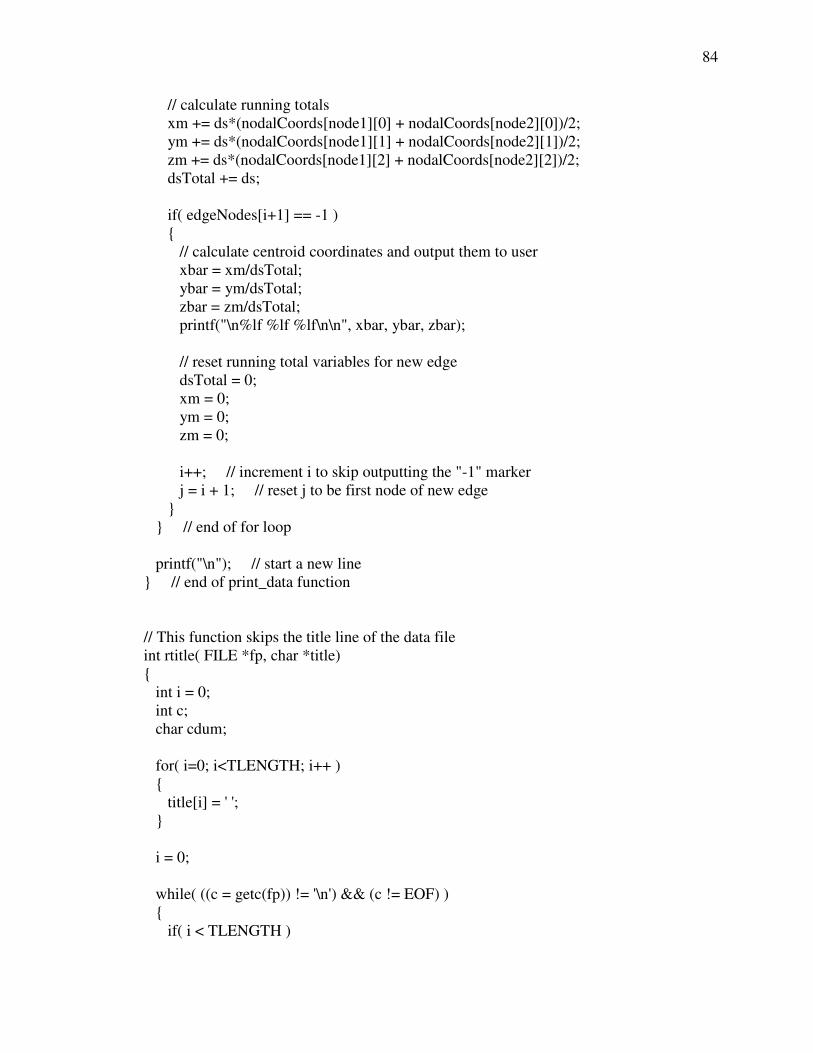
84
// calculate running totals
xm += ds*(nodalCoords[node1][0] + nodalCoords[node2][0])/2;
ym += ds*(nodalCoords[node1][1] + nodalCoords[node2][1])/2;
zm += ds*(nodalCoords[node1][2] + nodalCoords[node2][2])/2;
dsTotal += ds;
if( edgeNodes[i+1] == -1 )
{
// calculate centroid coordinates and output them to user
xbar = xm/dsTotal;
ybar = ym/dsTotal;
zbar = zm/dsTotal;
printf("\n%lf %lf %lf\n\n", xbar, ybar, zbar);
// reset running total variables for new edge
dsTotal = 0;
xm = 0;
ym = 0;
zm = 0;
i++; // increment i to skip outputting the "-1" marker
j = i + 1; // reset j to be first node of new edge
}
} // end of for loop
printf("\n"); // start a new line
} // end of print_data function
// This function skips the title line of the data file
int rtitle( FILE *fp, char *title)
{
int i = 0;
int c;
char cdum;
for( i=0; i<TLENGTH; i++ )
{
title[i] = ' ';
}
i = 0;
while( ((c = getc(fp)) != '\n') && (c != EOF) )
{
if( i < TLENGTH )

85
title[i] = c;
i++;
}
title[TLENGTH-1] = '\0';
return i;
} // end of rtitle function

86
REFERENCES
1. Abdel-Malek, Karim, Jingzhou Yang, Timothy Marler, Steven Beck, Anith
Mathai, Xianlian Zhou, Amos Patrick, Jasbir Arora. "Towards a New Generation
of Virtual Humans." International Journal of Human Factors Modelling and
Simulation, 2006: 2-39.
2. Denavit, J., and R. S. Hartenberg. "A Kinematic Notation for Lower-Pair
Mechanisms Based on Matrices." Journal of Applied Mechanics, 1955: 215-221.
3. Farrell, Kimberly, Timothy Marler, and Karim Abdel-Malek. "Modeling Dual-
Arm Coordination for Posture: An Optimization-Based Approach." Digital
Human Modeling for Design and Engineering Symposium. Iowa City: SAE
International, 2005. 2005-01-2686.
4. Fua, Pascal, Armin Gruen, Ralf Plaenkers, Nicola D'Apuzzo, and Daniel
Thalmann. "Human Body Modeling and Motion Analysis from Video
Sequences." International Archives of Photogrammetry and Remote Sensing.
Hakodate, Japan, 1998. 866-873.
5. Groβ, Clemens, Arnulph Fuhrmann, and Volker Luckas. "Automatic Pre-
Positioning of Virtual Clothing." Proceedings of the 19th spring conference on
Computer graphics. New York, NY: ACM, 2003. 99-108.
6. House, Donald H., and David E. Breen. Cloth Modeling and Animation. Natick,
MA: AK Peters, Ltd., 2000.
7. Jones, Peter R. M., Peng Li, Katherine Brooke-Wavell, and Gordon M. West.
"Format for human body modelling from 3-D body scanning." International
Journal of Clothing Science and Technology, 1995: 7-16.
8. Ju, Xiangyang, Naoufel Werghi, and J. Paul Siebert. "Automatic Segmentation of
3D Human Body Scans." IASTED International Conference on Computer
Graphics and Imaging 2000 (CGIM 2000). Las Vegas, NV, 2000. 239-244.
9. Kim, H., Q. Wang, S.F. Rahmatalla, C.C. Swan, J.S. Arora, K. Abdel-Malek, J.G.
Assouline. "Dynamic Motion Planning of 3D Human Locomotion Using
Gradient-Based Optimization." Journal of Biomechanical Engineering, 2008,
Vol. 130 / 031002-1.
10. Li, Peng, and Peter R. M. Jones. "Automatic Editing and Curve-fitting of 3-D
Surface Scan Data of the Human Body." Proceedings of the International
Conference on Recent Advances in 3-D Digital Imaging and Modeling. Ottawa,
Ontario, Canada: IEEE, 1997. 296-301.

87
11. Man, Xiaolin. A Mathematical and Computational Multiscale Clothing Modeling
Framework. PhD Thesis, Iowa City, IA: The University of Iowa, 2006.
12. Man, Xiaolin, and Colby C. Swan. "A mathematical modeling framework for
analysis of functional clothing." Journal of Engineered Fibers and Fabrics, 2007,
Vol. 2, Issue No. 3.
13. Man, Xiaolin, Colby C. Swan, and Salam Rahmatalla. "A clothing modeling
framework for uniform and armor system design." Modeling and Simulation for
Military Applications. SPIE, 2006. Paper No. 6228-10.
14. Mao, Chen, Sheng Feng Qin, and David K. Wright. "Sketching-out Virtual
Humans: From 2D Storyboarding to Immediate 3D Character Animation."
Proceedings of the 2006 ACM SIGCHI international conference on Advances in
computer entertainment technology. New York, NY: ACM, 2006. Article No. 76.
15. Marler, R. Timothy. A Study of Multi-Objective Optimization Methods for
Engineering Applications. PhD Thesis, Iowa City, IA: The University of Iowa,
2005.
16. Nedel, Luciana Porcher, and Daniel Thalmann. "Modeling and Deformation of
the Human Body Using an Anatomically-Based Approach." Computer Animation
98 Proceedings. Philadelphia, PA: IEEE, 1998. 34-40.
17. Nurre, Joseph H. "Locating Landmarks on Human Body Scan Data."
International Conference on Recent Advances in 3-D Ditial Imaging and
Modeling, 1997. Ottawa, Ontario, Canada: IEEE, 1997. 289-295.
18. Pargas, Roy P., Nancy J. Staples, and J. Steve Davis. "Automatic Measurement
Extraction for Apparel from a Three-dimensional Body Scan." Optics and Lasers
in Engineering, 1997: 157-172.
19. Rahmatalla, Salam, H. Kim, M. Shanahan, and Colby C. Swan. "Effect of
restrictive clothing on balance and gait using motion capture and dynamic
analysis." SAE 2005 Transactions Journal of Passenger Cars-Electronic and
Electrical Systems, 2006: Paper No. 2005-01-2688.
20. Rigotti, Camilla, Pietro Cerveri, Giuseppe Andreoni, Antonio Pedotti, and
Giancarlo Ferrigno. "Modeling and Driving a Reduced Human Mannequin
through Motion Captured Data: A Neural Network Approach." IEEE
Transactions on Systems, Man and Cybernetics - Part A, 2001: 187-193.

88
21. Seo, Hyewon, See-Jo Kim, Frederic Cordier, and Kyunghi Hong. "Validating a
Cloth Simulator for Measuring Tight-fit Clothing Pressure." Proceedings of the
2007 ACM symposium on Solid and physical modeling. New York, NY: ACM,
2007. 431-437.
22. Siebert, J. Paul, and Stephen J. Marshall. "Human body 3D imaging by speckle
texture projection photogrammetry." Sensor Review, 2000: 218-226.
23. Systems in Motion. Rational Reducer.
http://taylortrade.com/sim/rationalreducer.htm (accessed February 27, 2008).
24. TC Squared. TC2 - 3D Body Scanner Specifications.
http://www.tc2.com/products/body_scanner.html (accessed February 3, 2008).
25. Uicker, Jr., J. J., J. Denavit, and R. S. Hartenberg. "An Iterative Method for the
Displacement Analysis of Spatial Mechanisms." Journal of Applied Mechanics,
1964: 309-314.
26. Xiang, Y., H.J. Chung, A. Mathai, S. Rahmatalla, J. Kim, T. Marler, T., S. Beck,
J. Yang, J.S. Arora, K. Abdel-Malek, John Obusek. "Optimization-based
Dynamic Human Walking Prediction." 2007 Digital Human Modeling
Conference. Seattle: SAE International, 2007. 2007-1-2489.