
an analysis of the socio- economic benefit from day- ahead ...
116
I Analysis report Cables to Germany and the UK – an analysis of the socio- economic benefit from day- ahead trading General background to and basis for 2013 licence application
-
Upload
khangminh22 -
Category
Documents
-
view
2 -
download
0
Transcript of an analysis of the socio- economic benefit from day- ahead ...

I
Analysis report
Cables to Germany and the UK – an analysis of the socio-economic benefit from day-ahead trading General background to and basis for 2013 licence application

II
DISCLAIMER
15 May 2013 Statnett SF submitted an application for a licence under Section 4-2 of the Norwegian Energy Act to the Ministry of Petroleum and Energy for facilitation of international power trading for two projects. One of the applications relates to power trading with Germany, while the other deals with power trading with the UK.
We present the analyses of the socioeconomic benefit from day-ahead trading in a separate report attached to the application. The title of the report is «Cables to Germany and Great Britain – analysis of socioeconomic benefit from day-ahead trading».
The purpose of this English translation of the analysis report is to provide Statnett partners and the relevant authorities in Germany and the United Kingdom insight into the basis for the Norwegian interconnector license application. Since this version of the report may contain inaccurate translations, we want to emphasize that it is the Norwegian version of the report which is the official version.
Oslo, 28 June 2013

III

IV
INTRODUCTION
Statnett plans to build new cable power links with Germany and the UK before the end of 2020. In this report, we give our updated analysis of the socio-economic benefit to be had from use of the cables in the spot market. The analysis represents part of the basis to Statnett’s BP2 decision for the cable projects and the two applications for foreign licences.
In the report we present estimates of the anticipated Norwegian benefit in spot market trading and a sample space for this benefit. We discuss central drivers, areas of uncertainty, fundamental relationships and the cables’ impact on Norwegian electricity prices.
The planned projects involve considerable investments. For that reason we have for a number of years worked systematically on creating the analytical foundations on which to base our estimates of the benefit in spot market trading. What we present here is the outcome of an extensive series of partial analyses, where full use is made of our entire accumulated knowledge base. The work on the analysis will continue until the final investment decision is taken (BP3).
The report is authored by Eirik Bøhnsdalen, Anders Kringstad (project leader) and Lasse Christiansen from the Market Analysis unit of Nettdriftsdivisjonen (Power Transmission System Operation Division). Other major contributors to work on the analysis have been Amund Ljønes (project leader up until 1 December 2012), as well as Gavin Bell, Michel Martin and Erlend Torgnes from the analysis company Pöyry Norge, which has supported the analysis throughout the entire period. In our work on the capacity markets we have worked closely with Kristin Munthe and Halvor Bakke in the Market Design department of the Commercial Division. The responsible line manager is Bente Haaland, department manager for Power Systems Analysis.
Oslo, Norway, May 2013

V
SUMMARY
Statnett plans to build two new 1400 MW cables to Germany (2018) and the UK (2020), respectively. In this report we give our updated analysis of the socio-economic benefit to be had from use of the cables in the spot market. The analysis represents part of the background to and basis for Statnett’s application for foreign licences for the cable projects.
The future electricity prices we present in the report are not intended as some kind of forecast of future electricity prices, but result from the assumptions on which we base our expected scenario. There is considerable uncertainty about future price trends and we have therefore undertaken a large number of sensitivity analyses to check the robustness of cable benefit.
Anticipated annual benefit for Norway is EUR 120 to 160 million per cable
The cables to Germany and the UK provide the systems on both sides with greater flexibility, thereby giving us better utilisation of the combined power plant portfolio. This results in a considerable socio-economic gain for both Norway and our trading partners.
Thermal generation in Germany and the UK provides the Norwegian-Swedish power generation system with assistance in handling hydrological fluctuations, by producing more when it is dry and less when it is wet.
Regulatable hydropower in Norway and Sweden delivers short-term flexibility to the markets in Germany and the UK by relocating production in time.
Our estimate of the expected Norwegian benefit is EUR 120 to 160 million per annum per cable if the total transmission capacity is used in the spot trading market. The total Nordic benefit is greater, as Sweden in particular will stand to gain a lot from the Norwegian cables. From a Nordic perspective this reinforces the socio-economics of the projects.
The cables mean we obtain a somewhat lower difference in price hour for hour between Norway and Germany/the UK. At the same time, our analyses indicate that there will still be congestion and big price differences most of the time, even with a 1400 MW increase in trading capacity to each country. Both differences in price and more equal prices contribute to the socio-economic gain, in the form of congestion revenues and increased producer and consumer surplus, respectively.
Year 2020 2030
Country Germany UK Germany UK
Congestion revenue from cable 83 102 79 86
Other congestion revenues -21 -22 -20 -20
Increase in total Norwegian producer and consumer surplus 85 69 78 57
Total Benefit 147 149 137 123
Table 1: Our estimates for anticipated benefit in 2020 and 2030, using full cable capacity in the spot market. Figures in EUR millions.
As anticipated, we see a decreasing marginal benefit from increased transmission capacity out of the Nordic region. This has two important implications for our estimates:
We get a reduction in the congestion revenues for existing interconnectors. This pushes down the estimates for annual Norwegian benefit by almost EUR 20 million per cable.
The benefit of the cable to the UK will be reduced somewhat as it will be the second to be built, as cable number 2.

VI
This last point means that the congestion revenues we indicate for the Germany cable are higher than they will actually be if we build both of them. Once we build a cable to the UK, the congestion revenue on the cable to Germany is reduced, but to derive the marginal benefit of cable number 2, this reduction has been incorporated in the balance sheet for the cable to the UK, under the item “other congestion revenues”.
Different system characteristics result in a big gain from trading
The characteristics of the hydropower-dominated generating portfolio in Norway and Sweden are today fundamentally different from those of the thermal generating portfolio we find in Germany and the UK. We expect that there will continue to be major differences throughout the lifetime of the cables. This results in significant price differences hour for hour and is therefore the main reason why the cables deliver such considerable socio-economic gain.
In Norway and Sweden around 60-70% of current combined electricity generation is from hydropower, and of this almost 60% is regulated production. Regulated hydropower can alter production to match needs almost free of charge. The ability to store water over time also allows a lot of production to be relocated to periods when prices are higher. This results in considerably less short-term variation in price in the Nordic countries
1
than in Germany and the UK, where the high costs of regulating output from thermal power plants results in high price volatility. Between now and 2030-2050 we expect large parts of fossil-fuel generation to be replaced by unregulated solar and wind power. We do however expect that thermal power plants will continue to play an important role in price formation. Combined with a larger proportion of prices tending to zero as a result of more renewables, this will result in short-term price volatility in these countries far above that of Norway in the future as well. Different regulation costs are therefore an important driver behind the cables’ anticipated congestion revenues.
The large proportion of hydropower in the Norwegian-Swedish system has advantages, but also major challenges. First of all, a large part of the hydropower is unregulated, with the largest part of production being in the summer season when consumption is at its lowest. Secondly, the water inflow can fluctuate significantly from year to year. In Norway alone the annual inflow to existing hydropower plants can vary by around 60 TWh. To this must be added the effect of temperature fluctuations, which show a positive correlation with the fluctuations in inflow. Overall these challenges result in a big need for exchange capacity with neighbouring countries having the appropriate thermal production characteristics.
Looking to the future, the challenges in managing hydrological fluctuations will increase, especially in terms of successfully offloading overproduction by selling it. The three central drivers behind this are:
Greater surplus on the power balance in Norway and the Nordic countries
Expansion of more unregulated production
Fewer coal power plants in Denmark and Finland
We expect the surplus on the Nordic power balance to increase to 25-35 TWh in 2020-2030. Combined with more unregulated production when consumption is low, this means there is a big need for export in the summer season, and in particular in years where inflows are high. This increases the socio-economic benefit of the cables. We obtain greater congestion revenues, the net export is better paid and there is less risk of unutilisable water going to waste.
The cables help strengthen security of supply, even though an increasing power surplus initially reduces the role of the cables in ensuring energy accessibility in Norway and the Nordic countries. With a 2800 MW increase in exchange capacity, Norway can, if needed, import more over the shorter term and at a lower price than without the cables. Such a need may arise if we again encounter a period where there are problems with Swedish nuclear power production, combined with low inflows and winter temperatures.
1 By the Nordic countries we mean here mainly Norway, Sweden and Finland. Denmark has a pricing pattern
which is closer to that of the European continent.

VII
The cables impact on Norwegian prices and result in distribution effects between producers and consumers
The cables to Germany and the UK affect the prices in Norway and the Nordic countries in various ways. We have more stable prices throughout the year, but also more short-term price volatility. Since we expect a greater Nordic power surplus and more unregulated production, in isolation the cables will also result in a higher level of prices in Norway (averaged over the year). With the specific assumptions we have used in our base estimate, our simulations indicate that the average price in Norway will rise by just under EUR 5/MWh
2
(NOK 0.04/kWh) in 2020 and EUR 4/MWh (just over NOK 0.03/kWh) in 2030, in total for both cables. Nevertheless, it is not clear how big this effect will actually be and how long it will be maintained. If we get a lower Nordic surplus than we have assumed and greater transmission capacity to other systems, the prices will increase less. If, on the other hand, there is a trend in the opposite direction, the increase will be greater. In addition, the market may adjust to what is, in relative terms, a low price level if the cables are not built, by increased industrial consumption for example. If this happens, we get higher prices without the cables as well, and the cables’ real impact on the price level will be reduced. The exact extent of this kind of market adjustment remains uncertain, but if we get increased consumption of 5-6 TWh, our simulations indicate that the difference in price level with and without cables will be reduced to around EUR 3.1/MWh (NOK 0.025/kWh) in our main scenario for 2020.
Changed prices on the Norwegian side result in a big gain in the form of increased producer and consumer surplus. At the same time, this results in a redistribution between producers and consumers. Which of the two groups achieves a net gain is closely linked with how the prices are affected. Generally, in years and periods of surplus, where the price is initially low, the producers gain from there being cables. In years of deficit, when the price would otherwise be high, it is the consumers who stand most to gain from the cables being there. To the extent that future market trends can currently be identified, the cables are most likely to result in a redistribution from consumers to producers in the period up until 2020 and 2030. Nevertheless, the extent of this redistribution is not clear, as it depends on future trends in the power balance, the growth in exchange capacity between the Nordic countries and other systems, and the size of potential market adjustments if we do not build the cables. In addition to this, there will probably be variations as to which group achieves the net gain throughout the cables’ lifetime, due both to changes in market conditions and as a result of hydrological fluctuations.
It is important that we see the changes in price level and the distribution effects between producers and consumers in a wider context. First of all, changes in gas, carbon and CO2 prices have a big impact on Norwegian average prices, whether or not we build cables to Germany and the UK. Secondly, the price increase we obtain as a result of the cables should be seen in the context of the expansion in production from renewable sources. In combination with more nuclear power in Finland, this will initially drive down Nordic price levels. This reduces the redistribution from consumers to producers if we view renewables and cables together. Also, irrespective of the other market trends in the Nordic region, it may well result in consumers enjoying a net gain overall. Thirdly, the biggest increase in prices will clearly be in the wettest years. The increase in price we get with the cables is therefore not due to even price growth alone, but is also a consequence of more even prices over the year and between wet and dry years.
A multitude of areas of uncertainty results in a big sample space
Many of the most important drivers for the benefit from the cables are closely linked to the future development of the UK, German and Norwegian power generation systems, as well as those in Europe generally. Several of these are characterised by a significant degree of uncertainty in certain aspects, and overall this results in uncertainty in the estimates of anticipated benefit. Our analyses indicate that the following factors have the greatest importance:
The size of the Nordic power surplus throughout the year and in the summer season, and how long this will last
The price levels for thermal fuels and CO2 quotas
2 The exchange rate is NOK 8 per euro.

VIII
The number of cables from Norway and Sweden, and the effect of more flexible trading between Russia and Finland
The degree of flexibility of consumption in the UK, Germany and the other countries on the continent
The future capacity margin in Germany and the UK
System and market-related effects of an ever-increasing proportion of renewables in the generating portfolio of our trading partners
Further development of the power generation systems in Norway, the Nordic countries and Europe after 2030
In order to outline a possible sample space capable of enduring over much of the cables’ lifetime, we have in the light of this compiled a low and a high scenario for the cable benefit in both 2020 and 2030. In this we have consciously made adjustment for various factors which affect the benefit in either a downward or upward direction. This results in a sample space of an annual gain of EUR 70-90 million, between the low scenario and the high scenario, per 1400 MW cable.
We believe this provides a realistic picture of the uncertainty, but would emphasise that other compilations of assumptions are possible which would result in a bigger sample space. It is also important to note that the high and low scenarios are only an approximation of anticipated benefit in the event the market develops differently. Just as for the base estimates, any fluctuations in weather and fuel prices will again result in major deviations.
In our view our model simulations provide a representative picture of the situation up until 2030-2035. At the same time, weaknesses in the model and the data basis represent an area of uncertainty in our estimates. We have allowed for some of this by correcting the model results manually in those cases where we have the data available to do this.
The benefit is robust in spite of the uncertainty
We judge the benefit to be in the main stable and robust, in spite of the many areas of uncertainty. This is due to a number of things, including the fact that the cables open up trade in both directions, either in the form of more or less continuous flow one way or with frequent changes in the direction of flow. This flexibility means that the cables contribute to increased resource utilisation, and, as a result, high socio-economic gain, over a wide range of possible scenarios for future development.
Many of the most important drivers behind the benefit feature relatively low levels of uncertainty. So, for instance, already today we are encountering significant challenges in having to manage hydrological fluctuations, and hydropower has unquestionably great potential for relocating production in time and thereby delivering more short-term flexibility. On the European side, short-term price volatility may be either greater or smaller than at present, but it will still be bigger than in Norway or the Nordic countries.
In terms of future market developments, a lot does of course remain uncertain, but the main traits are nevertheless clear. Europe is on the way to re-adjusting her power generation system by incorporating a considerably larger proportion of production from renewable sources and lower GHG emissions. Norway and Sweden obtain more unregulated production via the certificate market, and it is likely that the Nordic countries as a whole will have a bigger power surplus. The question is more how big this surplus will be and how long it will last. This limits the uncertainty as regards cable benefit, particularly for the first ten years of the cables’ lifetime.
The great increase in combined producer and consumer surplus also has a stabilising effect on the benefit to Norway. This spreads the risk and means that several factors have to pull in the same direction if there is to be a big effect on the overall benefit. In addition, the increase in producer and consumer surplus, the congestion revenues and the losses on existing interconnectors are closely interconnected via the cables’ effect on Norwegian electricity prices. In periods where the effects on prices are small, practically the entire gain will be in the form of congestion revenue. The combined producer and consumer surplus and the congestion revenues on other interconnectors will remain more or less unchanged. When, on the other hand, we have periods where there are big price effects, congestion revenues will be lower and we lose a lot on existing

IX
interconnectors. This will however be offset by a big increase in the producer and consumer surplus. These interrelated factors contribute to making the Norwegian benefit more stable.
We assume that the CO2 market will be used as a policy instrument for reducing GHG emissions up until 2030-2050. Currently however prices are very low, and it is possible the CO2 market will play a smaller role in the future, in favour of increased use of other policy instruments. All things being equal, lower CO2 prices result in reduced electricity prices throughout Europe as a whole, and in isolation this exerts downward pressure on the anticipated gain from trading. At the same time, it is more likely that we will see greater and more lasting differences between the short-term marginal costs for coal and gas power generation. This contributes to increased price volatility in both Germany and the UK and drives up congestion revenues. Our analyses would therefore indicate that we only get a moderate drop of 10-20% in the total gain from trading if we assume the CO2 price to be zero and compare the result with our base estimates.
Our high and low scenarios indicate that we have a big sample space for cable benefit. It is however true that if we apply a combination of assumptions which result in either a very low or very high benefit, this is often indicative of market-related imbalances. And the greater the imbalances, the more likely it is that other market-based adjustments will occur which contribute to restoring the balance. Examples of such adjustments might be:
More flexibility in consumption in response to a development where we end up with greater price volatility in Germany and the UK.
Less new transmission capacity from Sweden to Poland and Germany in response to a lower power surplus in the Nordic countries and less price volatility on the continent.
These types of adjustment reduce the theoretical sample space for the benefit and also make the extreme cases less probable than our more balanced base estimate.


XI
CONTENTS
DISCLAIMER ..................................................................................................................................... II INTRODUCTION ................................................................................................................................ IV
SUMMARY....................................................................................................................................... V
CONTENTS....................................................................................................................................... XI
PART I CENTRAL DRIVERS BEHIND THE BENEFIT .......................................................................... 1 1 INCREASED TRADING CAPACITY RESULTS IN BETTER RESOURCE UTILISATION .......................................... 2
2 CABLES RESULT IN A SOCIO-ECONOMIC GAIN ................................................................................. 4
3 GAIN FROM TRADING DEPENDS ON FUTURE POWER GENERATION SYSTEMS ........................................ 12
4 MANY FACTORS AFFECT THE BENEFIT, BUT ONLY A FEW ARE REALLY IMPORTANT ................................. 22
PART II BASE ESTIMATES AND CENTRAL FEATURES OF THE BENEFIT ................................. 29
5 METHODS FOR CALCULATING BENEFIT ESTIMATES ......................................................................... 30
6 BASE ESTIMATES FOR EXPECTED BENEFIT IN SPOT TRADING .............................................................. 35
7 BIG VARIATIONS IN BENEFIT AND EXCHANGE PATTERN OVER THE YEAR ............................................... 38
8 EFFECTS ON PRICE ON THE NORWEGIAN SIDE LINK THE VARIOUS PARTS OF THE BENEFIT TOGETHER ......... 42
9 CONTINUED BIG PRICE DIFFERENCES RESULT IN HIGH CONGESTION REVENUES ..................................... 44
10 PRODUCER AND CONSUMER SURPLUS ACCOUNT FOR A LARGE PART OF THE TOTAL BENEFIT ................... 48
11 THE BENEFIT DIMINISHES WITH MORE CABLES .............................................................................. 55
12 FLUCTUATIONS IN WEATHER AND FUEL PRICES INCREASE THE EXPECTED BENEFIT AND RESULT IN A BIG
ANNUAL VARIATION .......................................................................................................................... 58
PART III PRICE AND DISTRIBUTION EFFECTS................................................................................... 62
13 THE CABLES ARE ONE OF SEVERAL FACTORS WHICH AFFECT ELECTRICITY PRICES IN NORWAY ................... 63
14 THE DIRECT PRICE EFFECTS ARE A HIGHER PRICE LEVEL, GREATER STABILITY OVER THE YEAR AND AN INCREASE
IN 24-HOUR VARIATION .................................................................................................................... 65
15 LONG-TERM MARKET ADJUSTMENTS CAN REDUCE THE PRICE EFFECTS ................................................ 70
16 PRODUCERS EARN MORE ON AVERAGE, AND CONSUMERS GET BETTER SECURITY OF SUPPLY ................... 72
PART IV UNCERTAINTY AND SAMPLE SPACE .................................................................................... 76
17 METHODS FOR DEALING WITH UNCERTAINTY ............................................................................... 77
18 SCENARIO UNCERTAINTY .......................................................................................................... 80
19 WEAKNESSES IN MODEL, METHOD AND DATA BASIS RESULT IN UNCERTAINTY ...................................... 89
20 CALCULATED SAMPLE SPACE FOR THE NORWEGIAN BENEFIT ............................................................ 92
21 ROBUST BENEFIT IN SPITE OF THE UNCERTAINTY ........................................................................... 101


Page 1 of 104
Part I CENTRAL DRIVERS BEHIND THE BENEFIT
By building cables to Germany and the UK we obtain better utilisation of the combined power plant portfolio on each side of the cables. This is a fundamental reason why the cables deliver a socio-economic gain. How big a benefit we get depends on the characteristics of the systems we link together.
However, the entire European power generation system is in the middle of a massive readjustment process. The socio-economic benefit of the cables to Germany and the UK is therefore a function of systems with characteristics different from those we have had historically. Our analysis is therefore directed both at providing an overview of the future development of the power generation system in north-west Europe up to 2030-2050 and at outlining how this will affect the socio-economic benefit.
In this first part we first take a look at the fundamental relationships that underpin the socio-economic benefit. We then provide a brief outline of our main assumptions about the development of the entire power generation system in north-west Europe up until 2030.

Page 2 of 104
1 INCREASED TRADING CAPACITY RESULTS IN BETTER RESOURCE UTILISATION
By building cables to Germany and the UK we obtain better utilisation of the combined power plant portfolio on each side of the cables. This is a fundamental reason why the cables result in socio-economic gain. At a higher level, the increased resource utilisation is due to two main mechanisms:
Regulatable hydropower in Norway and Sweden uses its ability to relocate production in time and thereby delivers short-term flexibility to the markets in Germany and the UK.
Thermal generation in Germany and the UK provide the Norwegian-Swedish system with assistance in handling hydrological fluctuations, by producing more when it is dry and less when it is wet.
The cables therefore mean the systems on both sides have greater flexibility and lower operating costs. Since the flow can go both ways, either almost continually so or with frequent changes in direction of flow, the cables will help achieve increased resource utilisation over a wide range of possible scenarios for future development.
1.1 Norway gets help in managing her surplus and hydrological fluctuations
In Norway almost all electricity generation is based on hydropower. The Norwegian system is therefore dependent on trading with our neighbours if we are to be able to manage hydrological fluctuations. In Norway alone the inflow can vary by around 60 TWh between dry and wet years. To this must be added the effect of temperature fluctuations, which show high correlation with the fluctuations in inflow. This means that years and periods of low inflow often occur at the same time as relatively high consumption due to low temperatures, and vice-versa.
Norway currently has interconnectors to Sweden, Finland, Denmark and the Netherlands, and these play a crucial role in ensuring supply is secure in dry years, and avoiding unutilisable water going to waste in wet years. Looking to the future, the challenges in managing hydrological fluctuations will increase, especially in terms of successfully offloading overproduction by selling it. The three central drivers behind this are:
Greater surplus on the power balance in Norway and the Nordic countries
Expansion of more unregulated production
Fewer coal power plants in Denmark and Finland
The first two points increase the export need, particularly in the summer season, and, without increased outward exchange capacity from the Nordic system, it will be difficult to avoid unutilisable water going to waste in wet years. The coal power plants in Denmark and Finland have traditionally helped contain the hydrological fluctuations in Norway and Sweden by producing a lot in dry years and not so much in wet years. We anticipate that many of these will be decommissioned over the course of the next 10-20 years, thereby increasing the pressure further on the current outward interconnectors from the Nordic countries. To this should be added climate changes which will likely result in higher production in existing hydropower plants and lower consumption within the general supply.
With the cables to Germany and the UK we get a significant increase in outward exchange capacity from the Nordic system. This will make it easier to manage hydrological fluctuations in both Norway and Sweden.
1.2 Regulatable hydropower reduces production costs in Germany and the UK
Regulated hydropower can alter production to match needs almost free of charge. Large reservoirs mean also that water can be stored for production at a later time when prices are higher. In combination with the big market share
3, these characteristics result in relatively similar prices both over 24-hour periods and between
the seasons in Norway, Sweden and Finland. On the continent, the situation is different, with significantly
3The combined proportion of hydropower in Norway and Sweden is 60-70%. Of this, around 60% is regulated,
with the possibility of storing water in reservoirs.

Page 3 of 104
greater short-term price variations driven by high start-up and shutdown costs at the thermal power plants and fluctuations in the fuel prices.
With the new cables, regulated hydropower in Norway and Sweden will increase its production when the prices are highest in Germany and the UK, and we get full export. By the same token, they will reduce production when prices are low at our trading partners, and in this situation we then either import electricity or have lower export. Currently this adheres to a clear day/night pattern where we have high hydropower production and export during the day and the reverse at night. Over the longer term, the producers will also have greater opportunities for relocating production from periods where there is a lot of wind and solar power generation to periods where the situation is reversed. Either way, the principle is the same. We get increased utilisation of the hydropower plants’ ability to relocate production over time.
The interaction with regulated hydropower in Norway and Sweden helps reduce production costs in Germany and the UK. This is due to a number of factors, including the fact that fewer thermal power plants have to start up and shut down to cover fluctuations in demand and electricity generation from renewable sources. Full export from Norway means that less thermal power plants have to start up to cover peaks in consumption, whereas full import allows shutdowns of short duration to be avoided during low-load periods
4. The overall
result is lower operating costs.
1.3 The cables result in greater flexibility on the road to a decarbonised power generation system
The European power generation system is in the middle of major readjustment where thermal fossil-fuel production is being replaced by renewable production technologies. We will shortly return to this in more detail, but would here just mention that the cables also help make this process more efficient.
A central aim of restructuring the European power generation system is to achieve a dramatic reduction in GHG emissions from the power sector, as well as to help other sectors achieve reductions via electrification. To ensure this proceeds at a quick enough pace, production from renewable sources is, for instance, subsidised, and in Norway and Sweden the certificate scheme will result in a 26 TWh increase in production by 2020. Much of this can gradually be used for electrification within the oil, transport communications and heating sectors. The challenge arises when this does not take place as quickly as growth in production. In that situation we get a surplus, and this is where the cables play a big role in achieving sales of the power we exchange, until such time as domestic consumption perhaps picks up.
Moreover, in Germany and the UK the cables will make it easier to effect the transition to systems which are based to a much greater degree than today on production from renewable sources. These are bound to be big systems and a cable to Norway will therefore be of crucial importance. In the meantime the new interconnectors bring more flexibility in managing a relatively rapid restructuring process involving a significant probability of various forms of imbalance before it runs its course.
4 By low-load here we mean consumption minus production from renewable sources

Page 4 of 104
2 CABLES RESULT IN A SOCIO-ECONOMIC GAIN
2.1 The electricity market converts increased resource utilisation into socio-economic gain
New cables to Germany and the UK result in better resource utilisation. The gain derives first and foremost from better utilisation of the combined generating plant on both sided of the cables.
Figure 1 illustrates how this happens in principle. The production costs saved in the area with the highest price opened up by trading are considerably lower than the increased costs in the area with the lowest price. The difference between savings on costs in A and increased costs in B are the gain from trading. Which system out of the Norwegian hydropower-dominated system and the thermal generating systems in the UK and Germany has the lowest costs will vary over time. The typical pattern at the moment is that costs are lower in Norway during the day, with the reverse being the case at night. In future this will be more dependent on the weather. In periods where there is a lot of wind in winter, wind power may replace more expensive hydropower, which can be exported back at a later point and reduce start-up and shutdown costs in thermal plants.
There will always be a gain from increasing the capacity between two areas with different prices. The greater the difference in price the greater the gains from trading, as the prices in a properly functioning electricity market represent the costs of the resources needed to cover consumption.
The potential for more trading also results in more equal prices at each end of the cable. Figure 1 demonstrates the fundamental relationships underlying this equalisation. In the area with the highest price we get a price reduction due to production in units with the highest marginal costs being replaced by increased production from the area with the low price. More production in the low price area will however often push up the prices there, as increasing production is generally associated with a gradual increase in costs. This means prices will become more equal, while the benefit of increased transmission capacity diminishes. How quickly this happens depends on how steep the two curves are and how big the transmission capacity is.
Figure 1: Here we show how trading provides potential for replacing expensive production in area A by cheaper production from area B. FA and FB are the production volumes in each of the two areas prior to
trading. FA minus import and FB plus export indicates the production distribution with trading. As we see, area B covers more of the total production with trading, and there is a decrease in overall production costs.
The gain in real economic terms is realised via the electricity market. Provided there is free and efficient competition, the market keeps overall production costs to a minimum within all the limitations resulting from the transmission system and generating plant. This results in automatic utilisation of the new possibilities for reducing costs we get via the cables to Germany and the UK. This relationship is also the main reason we can use market models to calculate the overall benefit.

Page 5 of 104
2.2 Both price differences and more equal prices result in gain
In specific terms, the socio-economic gain becomes evident via:
Congestion revenues
Producer surplus
Consumer surplus
Congestion revenue, which is the difference in price multiplied by transmitted volume, accrues to the cable owners. This can be seen in that the cable owners buy electricity cheaply on the market at a low price and sell it at a profit on the market at a high price. Since there is a change in the prices due to the cables, the congestion revenues for all other interconnectors will also be affected. These changes are a part of the socio-economic balance sheet, in addition to the points above.
The producer surplus in one hour is the price the producers get, minus the production costs. The consumer surplus reflects the difference between the electricity price and the willingness to pay. With the cables, the difference in price between Norway and Germany/the UK will be smaller, as Figure 1 illustrates. This results in a socio-economic gain in that the overall producer and consumer surplus will be greater. From a Norwegian perspective a somewhat simplified explanation for this might run as follows. In hours where we import, we will be able to buy electricity cheaper from the continent than we can produce it ourselves. In hours when we export, we can sell the electricity at a higher price than we would otherwise have done. The former results in increased consumer surplus over and above what the producers lose. The latter results in increased producer surplus over and above what the consumers lose.
To calculate the increase in the overall producer and consumer surplus, we take the difference between model simulations with and without incorporation of the cables. This is a complicated calculation, as it depends on the price changes in all hours and where exactly in the system the production response occurs, which itself depends on a number of factors, including congestion in the grid. Both of our two market models
5 have
separate modules which calculate the socio-economic surplus on an hour-for-hour market equilibrium basis. When we take the difference between overall surplus before and after, we get the net gain. The figures we refer to in the report are annual net gain as an average of simulations over 47 historical inflow years. An inflow year consists of 2,912 observations
6.
The producer and consumer surplus is closely linked with the exact price effects which occur at a given time in the various systems as a result of trading. It should be pointed out that this may vary hour for hour over the year and between years. There are three main ways in which prices change in Norway:
We get more of a price difference over a 24-hour period as regulation resources become scarce in Norway
We get less of a price difference between the seasons
The average price level may change
Provided the balance between annual production and consumption is tolerable, we normally get equalisation of the effects on price in the long run, so that the effect on the average level will be moderate. More export during the day offsets more import at night and dry and wet periods even each other out. If, on the other hand, the Nordic countries experience major imbalances between consumption and production in a normal situation, the cables will also affect the average price level.
5 The EMPS model and BID (Better Investment Decisions).
6 In the EMPS model three hours are compressed into one hour, with the result that there are 56 price periods
in one week.

Page 6 of 104
2.3 The benefit tends to decrease with increased capacity and affects different locations at different times
In Figure 1 we see that the costs saved due to more trading decrease in proportion to increases in transmission capacity. This indicates that the benefit of trading tends to diminish. Figure 2 illustrates what happens when capacity increases to the point where there is no longer a difference in price over one hour. The projects currently being planned result in big incremental increases in capacity, so, although the linear curves are a simplification, they do illustrate what happens when capacity increases.
Figure 2 shows the diminishing benefit of more transmission capacity. When there is still a difference in price over one hour, the gain from trading is realised in the form of congestion revenue and market profit. In those hours when the cables result in absolutely equal prices, all profit accrues to the market actors in the form of
increased producer and consumer surplus.
The benefit declines gradually at the same time as more and more profit accrues to the market actors. Once capacity becomes so high that the prices are equal for an hour, all of the gain from trading has been realised. This also means that all of the profit accrues to the market actors. As far as trading between the Nordic countries and Europe is concerned, for many hours we will be in a situation where the figure to the left is the one that counts. There are nevertheless periods where we can see that the cables have a relatively big impact on prices. We will return to this later in the report.

Page 7 of 104
Figure 3: As the impact of cables on prices increases, the result is a more rapid decline in benefit from transmission capacity, as well as more benefit coming in the form of profits for market actors rather than
congestion revenue.
How big the impacts on price will be depends on the gradient of the red curve above. If the impacts on price are small for an hour, the benefit only diminishes slightly and most of it will be in the form of increased congestion revenue. In Figure 3, this is illustrated on the left. It also means that the gains from trading are split more or less equally between Norway and her trading partner provided the ownership share is 50/50. Nevertheless, it will be the case that even where there is a marginal impact on price, producer surplus in Norway may grow slightly. The reason for this is that we already currently have a degree of price structure. Increased exchange capacity means that regulated hydropower can move more production from low price periods to high price periods. This volume effect means that producer surplus may grow without this being at the expense of the consumer, even where the effects on prices are limited.
However, impacts on prices increase the proportion of the benefit which accrues to the market actors, resulting in more rapidly diminishing benefit from trading. This is highlighted by the fact that the area in the figure on the right is considerably smaller than that in the figure on the left. The fact that more of the benefit accrues to the market actors also means that distribution effects occur internally in Norway and between Norway and her trading partners.
In Norway, impacts on price result in both socio-economic gain and distribution effects between producers and consumers. We should also point out that the distribution effects between producers and consumers is very much greater than the gains. “Profit and loss” for the two groups will however largely be mutually offset, so the gain for Norway will derive from foreign trade. Over time it will be the power balance over the year which will be most telling in respect of the distribution between producers and consumers. A surplus during a normal year results in redistribution from consumers to producers, whereas a deficit has the opposite effect.
2.4 Congestion revenues are driven by volatility on the continent and a varying level in Norway
As already explained above, congestion revenues are a direct consequence of the fact that we link up with markets that have a different price. In general, there are two drivers underpinning this difference in price:
Whereas regulatable hydropower results in a relatively flat price structure over a 24-hour period in the Nordic countries, Germany and the UK have big short-term price volatility as a result of differences in short-term marginal costs, high start-up and shutdown costs in thermal power plants and varying demand.
At certain periods, varying hydrology results in significant differences in price level between the Nordic countries and the continent.

Page 8 of 104
Figure 4 Prices in a representative week for the entire 2009-2012 period, winter 2011 and summer 2012.
In normal hydrological situations it is the degree of price volatility among our trading partners which is the main generator of congestion revenues on the cables. This is illustrated in the figure on the left with historical prices from the whole of the 2009-20012 period. The average price in this period was only EUR 5/MWh higher in Germany.
On the other hand, in periods where there are hydrological imbalances where the price level in the Nordic countries differs significantly from the continent, differences in price level are the main source of increased congestion revenue with more cables. In these cases, the price level on the continent is also of great significance for the congestion revenues. This applies to dry periods in winter where there is a big need for import, as illustrated by the prices for winter 2010/2011, and to wet years or wet periods during the summer season, illustrated by the prices for summer 2012.

Page 9 of 104
2.5 Producer/consumer gain is greatest in periods of hydrological imbalance
The effects on producer and consumer surplus are greatest in periods where cables have a big impact on prices in Norway. This typically occurs in situations where hydrological conditions are critical to the price. In such situations, the flow on the interconnectors to our neighbours is usually continuous, in the form of either imported or exported power. In such cases quite small increases in transmission capacity can have a big impact on price levels:
In wet periods when there are high unregulated inflows, more trading capacity can mean that hydropower plants with a regulation capability will determine prices as opposed to unregulated production doing so. In addition, better capacity can raise water values in regulated hydropower. Both of these items will lead to an increase in prices in Norway.
In cold, dry winters where there is high consumption, a high import level and high prices in Norway, more import capacity will allow Norway to keep her position in balance at a lower cost. This will push down price levels in Norway.
The greater the imbalance, the more cable capacity is needed to trade out of the differences in pricing.
The other factor which determines the impact of hydrology in Norway is the price structure on the thermal side. In situations where Norway depends on continuous import, Norwegian prices may rise to such an extent that they are higher than the peak prices on the continent, irrespective of how high these may be. In winter 2010/2011, for instance, these peak prices were relatively low, so that Norwegian price levels in Norway only had to rise to just over EUR 60/MWh to result in full import. On the other hand, German/European prices at night determine how much Norwegian prices have to fall to result in full export during periods of big inflow
7.
Later on we will see that much of the hydropower production in Norway/the Nordic countries in summer is forced production which cannot be moved between different seasons. With a growing power surplus, driven, among other things, by still greater unregulated summer production, the situation on the right in Figure 4 will become even more dominant in terms of cable benefit than it has been historically.
2.6 The producer/consumer surplus effect is big in periods when we approximate to continental price patterns
We also see considerable effects on producer/consumer surplus in periods where the cables have a big impact on prices directly, without this being driven by hydrological conditions in the Nordic countries. This usually occurs as a result of power shortages in Norway both in terms of covering all her consumption and of exporting to her neighbours. We currently see this happening when consumption in Norway is around 21,000-22,000 MW. Having more cables will mean we more rapidly reach a level of consumption where we get a price pattern which is more like that of our trading partners.
Export will always be reduced first to the area which has the most similar price, typically Sweden8. If this proves
insufficient, the Norwegian price will increase until we have reduced our export to whichever of our other trading partners has the lowest price. This process continues until we are under the output ceiling in Norway. The number of cables on which export has to be reduced is determined by the distribution between congestion revenue and producer/consumer surplus. If export has to be cut even to the country with the highest price, all benefit comes in the form of producer/consumer surplus.
The greatest producer/consumer gain will however occur if a power shortage occurs in the sense of there not being enough output
9 in the Norwegian/Nordic system to cover our own consumption. This will result in very
7 Here we should also mention that there can be big fluctuations over shorter periods. In winter 2011, price
levels were on average EUR 18/MWh higher in Norway than in Germany, whereas in winter 2012 they were EUR 10/MWh lower. 8 That is, of course, provided we are not importing any power.
9 The sum of available production capacity and import capacity.

Page 10 of 104
high prices, determined by the price for various actors having to cut their consumption. In such cases increased exchange capacity can significantly reduce the prices, thereby resulting in very big gains for consumers.
In periods where there is very low consumption, we can also import the prices directly from the continent. These till typically be low. This will however occur more infrequently, as in these situations we tend to have forced export. In such cases the price on the continent will be relevant to determining the export price.
2.7 Cables to Germany and the UK would have brought high levels of benefit over the last 10 years.
The historical differences in price with Germany and the UK during the last 10 years are a good indicator of how profitable cables would have been in socio-economic terms. These differences indicate that the gains from having more trading capacity would have been considerable. They also show the considerable revenues achieved from electricity trading between Norway and the Netherlands since NorNed came on line in May 2008. Statnett’s share (50 per cent) of congestion revenue since the cable came on line in May 2008 until the end of 2012 has been around EUR 185 million. We also know that the socio-economic gains have been considerably greater than just the congestion revenue for Norway, as the cable has been of great value to market actors in Norway. This is however difficult to quantify. An estimate based on model simulations points to the additional socio-economic gain from the cable
10 having been at least EUR 90 million. In winter
2010/2011, moreover, import from the Netherlands, nearly 2 TWh, was important to avoid running out of water/rationing.
The differences in price are due to periods where there is a lot of price volatility as well as periods where there are big differences in price levels. The latter are driven primarily by hydrological imbalances (see Figure 4). When these coincide with high fuel prices, as they did in 2008, this can result in a very high Norwegian benefit. The significant revenue from NorNed over this period is also due to a reduction in capacity from Southern Norway to Denmark and Sweden, resulting in a lot of confined power.
Figure 5: The Norwegian share of estimated congestion revenue for a 1400 MW cable based on price differences between Norway and Germany and Norway and the UK during the period 2002-2012. Figures are
at the currency rate current at the time in question.
Figure 5 shows the Norwegian share of estimated congestion revenue for a 1400 MW cable to either Germany or the UK based on historical price differences. We have adjusted income down by 20 per cent per annum to allow for loss on the cables and a general estimate of price effects on the Norwegian side. On average, over the entire period this results in congestion revenue of EUR 78 and 92 million per annum for Germany and the UK, respectively.
10Increased producer/consumer gain minus decrease on existing interconnectors

Page 11 of 104
Considering that we have corrected congestion revenues downwards by so much to allow for impact on prices on the Norwegian side, this means that the cables in the same period will result in a significant gain in the form of producer and consumer surplus. The total Norwegian benefit will therefore be more than our estimate for historical congestion revenue.

Page 12 of 104
3 GAIN FROM TRADING DEPENDS ON FUTURE POWER GENERATION SYSTEMS
How big the socio-economic gain we get via spot trading on the cables to Germany and the UK depends on the characteristics of the systems we link together. However, the entire European power generation system is in the middle of a massive readjustment process. This affects the potential for profitable trading and means that we cannot base our analysis on historical and current power generation systems alone. The objectives of our analysis here are therefore twofold:
To provide an overview of the main traits in the development of the power generation system in north-west Europe towards 2030-2050.
To gain an insight into how this affects the socio-economic benefit.
In this chapter we provide a brief outline of our main assumptions about the development of the entire power generation system in north-west Europe up until 2030. We have chosen to base our analysis on a central scenario and various sensitivity analyses using the latter as starting point. This scenario represents what we believe is the most likely path future development will take until 2030-2050. Using this scenario as a framework we have assembled a central dataset for 2020 and 2030, respectively. These datasets are a detailed specification of our assumptions about more general traits of development and provide a consistent and balanced starting point for our analyses of the benefit deriving from the cables.
3.1 Big changes in the European power generation system between now and 2030-2050
The European power generation system is in the middle of a long drawn-out process of extensive readjustment to becoming a system which will produce considerably lower GHG emissions. The EU’s objective to achieve an overall reduction in GHG emissions of 20 and 80 per cent by 2020 and 2050, respectively, involves more or less total decarbonisation of the power sector. By 2030, the power sector must have already reduced its emissions by 50 to 60 per cent if the target for 2050 is to be achieved. For the systems in the UK and on the continent, which up until now have largely been based on fossil-fuel thermal production, this will mean a radical change.
Fossil-fuel electricity generation, first coal and then gas, must be replaced by emission-free technologies.
The power sector must contribute to cuts in other sectors, by electrifying transport communications and heating, for instance.
The power grid requirement is growing, both in terms of being able to transport the renewable electricity for consumption and being able to handle the big fluctuations in production from renewable sources.
Although there is a good deal of uncertainty and many different views as to the rate of this change and how it can actually be achieved in terms of its specifics, we are of the opinion that it is likely European countries will go further in implementing big cuts in emissions than the rest of the world. We take this view for a number of reasons, including the following:
Europe has already made a good start. Specific emissions targets have been set for 2020, both the EU and national agencies have established the necessary policy instruments to achieve these targets, and many countries are well down the road to increasing the proportion of renewables in their generating portfolio.
The EU and the governments of the individual states repeatedly confirm their intention to continue with this policy. Thanks to big reforms such as Energiewende and EMR
11, Germany and the UK,
respectively, are converting their policy objectives into specific, binding measures. Here a great deal of discussion is still ongoing about both the targets and the policy instruments used to achieve them, and
11 Electricity Market Reform

Page 13 of 104
there are several opposing forces of no small influence which would like to see things develop in a different direction. At a general level, however, there is little which indicates that there will be any significant change in policy.
The energy policy in European countries uses a number of arguments to support a vision of a carbon-neutral society. Perhaps the most important of these is the need to reduce dependency on energy imports from countries outside the EU. Re-structuring in Germany is in addition driven by the decision to phase out nuclear power.
Both Germany and the UK are at the forefront of this development. As stated above, the UK has set about implementing a major reform of the electricity market (the Electricity Market Reform), where the central objective is to ensure a cut in emissions within the power sector in accordance with the EU’s climate targets for 2050. The reform has been largely designed to ensure the necessary investments in emission-free production and thermal back-up capacity, and consists of four parts.
A price floor for CO2 emissions, as an addition to the EU’s quota market.
An upper limit for GHG emissions from new power plants, over and above the requirements enshrined in the EU LCPD and IED Directives. The limit has been set so low that it will not be possible to build new coal power plants.
A subsidy scheme for renewables and nuclear power, adapted to the individual technology.
A capacity market to ensure the necessary investments are made in thermal back-up capacity.
Overall, EMR creates long-term stability for investors, thereby rendering it possible to achieve the emission cuts targets at the same time as ensuring security of supply.
Germany has for several years been a country which leads the field in cutting GHG emissions within the power sector. The country has robust support schemes for renewables and within just a few years has developed large quantities of wind and solar power. At the end of 2012, total installed power was round 60,000 MW, with roughly equal distribution between the two technologies. This amounted to a renewables proportion of just over 20% of total electricity generation in 2012, and Germany is therefore well on course to exceed the requirements for the proportion of renewables set out in the EU’s 20-20-20 targets. Similarly, after the nuclear accident in Fukushima, Germany also passed a resolution to phase out nuclear power by 2022, further increasing the need for production from renewable sources. Given that the much of the production from renewable sources is in the north, there is also a radical increase in transmission need. Germany has therefore recently adopted an extensive plan to enhance the power grid by 2022, the same year as the last reactor will be decommissioned. The entire package with decommissioning of nuclear power, the transition to renewables and associated grid expansion is referred to by the term “Energiewende”. The targets and strategies for “Energiewende” are soundly based on a broad political consensus.
When it comes to the Nordic power generation system, the EU’s energy and climate policy provides strong guidelines for its development, with decarbonisation and increased integration as the dominant development trends up to 2030. This is reinforced both by existing expansion plans and by national policy objectives. Nevertheless, we will not witness such a big upheaval in the Nordic system, as the proportion of emission-free production is already so high at the outset. On the other hand, we will have more unregulated production, even less thermal production and a larger total power surplus.
3.2 Policy objectives, expansion plans and our own analyses provide a starting point for our specific assumptions
Our assumptions relating to the future development of the power generation systems in north-west Europe are based largely on the European states implementing the major part of their climate and energy policy, as we have outlined in the previous section. To be specific, we are assuming that the countries in north-west Europe will be in a position in 2030 where they can meet the EU’s emissions targets for 2050. This involves a reduction in emissions of around 60% from their 1990 level.

Page 14 of 104
In addition, we use specific policy objectives and expansion plans as a basis for advancing a few steps beyond today’s system. Some examples of this are:
Known expansion plans: Database of all existing power plants in Europe, including those due for definite expansion and decommissioning (Pöyry)
National Renewable Action Plans (2020)12
and EU roadmap 2050
Laws and directives associated with emissions and approvals for new power plants (LCPD, IED, EMR)
One challenge in using known expansion plans as a basis is that many of them are mutually dependent. So, for instance, we cannot simply add up all plans for new power plants, as this would result in unrealistically high over-capacity in the market. In the process of fleshing out and analysing future development we therefore employ some basic assumptions as references:
Most countries control their energy policy along the lines of becoming “self-sufficient” in terms of electrical power
13.
The electricity market is efficient and the actors on it behave rationally in economic terms.
Various agency bodies impose requirements on security of supply and ensure these are met.
The cuts in emissions will be made with the aid of a fairly well balanced and cost-effective use of a number of policy instruments: phasing out of coal, regulation, CO2 price, construction of new renewable generating plants and more transmission capacity.
As far as possible, we will attempt to justify all our choices on the basis of our own analyses, external reports or other data sources. To make sure our detailed assumptions are internally consistent, we will use model simulations to check out relationships and discover any conflicts. Typical aspects which we will check are the extent to which there is sufficient production to cover demand, whether new power plants will be sufficiently profitable and that simulated emissions meet our assumptions about emissions cuts.
3.3 Renewables and, to some extent, nuclear power replace coal and gas on the continent and in the UK
Figure 6 provides an overview of the development in the capacity mix in our dataset up until 2030. At a general level we assume that the proportion of production capacity from renewable sources will grow at the expense of fossil thermal capacity, in particular coal-fired power.
12 National plans for how the individual member state is to meet the requirements set in the EU’s 20-20-20
targets 13
This applies to both output and energy production over the year, but will only have an impact on persistent major imbalances.

Page 15 of 104
Figure 6 Development in the capacity mix in the UK, Germany and combined for our modelled area outside of the Nordic countries
There is currently a relatively big difference in the capacity mix between Germany and the UK. Germany has a more diversified capacity mix, where renewables and emission-free production represent a much bigger proportion overall. In terms of fossil fuel they also have a lot of lignite (brown coal). On the other hand, the UK has a lot more gas power based on CCGT, more coal power and a lower proportion of renewables.
Keeping the Nordic countries out of it for the moment, we assume that combined production capacity from renewable sources for the entire area we have modelled
14 will grow from 160 GW in 2012 to 300 GW in 2020
and 440 GW in 2030. In Germany we have distributed the growth between wind and solar power. In 2030 this will give total installed power from renewable sources of 130 GW, i.e. more than 50 per cent of the country’s production capacity. The UK is investing more in wind power, and we are assuming that by 2030 they will have a capacity in renewables of 55 GW, equivalent to 40 per cent of their total installed power.
Coal power is the production technology which will see the biggest reduction, and by 2030 most of it will have been phased out, both in Germany and the UK. In addition we expect that Germany will phase out lignite by 2030, although there is currently no clear decision on that. As regards gas power, some growth is expected to meet shortfalls in the varying production from renewable power plants. Germany and the UK will have 20 and 40 GW, respectively, in CCGT in 2030.
The changes give both countries more of a similar capacity mix as 2030 approaches, but there are still many differences. Among other things, we are assuming there will be more nuclear power in the UK after 2020, as opposed to Germany, which will be phasing it out entirely by 2022.
3.4 Moderate growth in consumption by 2020, more by 2030
In our dataset for 2020 we have used the NREAP figures15
for growth in consumption on the continent. The NREAP figures cover a number of things, including 2020 targets for energy efficiencies. In Germany this results in a decline in consumption of 30 TWh from 2012, and in the UK a decrease of 10 TWh, whereas in the rest of the modelled area, there is an increase of around 100 TWh. Overall the consumption outside the Nordic region is more or less at the same level as in 2012. This also reflects uncertainty as to how Europe will develop in economic terms.
Figure 7: Consumption in 2012, 2020 and 2030 in our base scenario
Figure 8: Consumption trends from 2020 to 2030 by category
Over the long term there are three features of future development which are most important for consumption:
14The UK, France, Belgium, the Netherlands, Germany, Switzerland, Austria, Czech Republic, Poland and the
Baltic States 15
National Renewable Energy Plans

Page 16 of 104
Energy efficiencies
Electricity may increase its share of energy end-consumption. Currently this stands at approximately 20 per cent.
Economic growth and the ability of industry to compete
From 2020 to 2030 we are assuming growth of just above 10 per cent in total consumption, in spite of energy efficiencies. There is great potential for energy efficiencies, but it is uncertain how much of the potential will be realised. We are assuming the efficiencies will reduce consumption by approximately 5 per cent from 2020 to 2030.
Overall this will increase power consumption by around 8 per cent from 2020 as a result of economic growth. The estimates for economic growth have been obtained from the World Bank, whereas the growth in power consumption this generates has been derived from consumption elasticities provided by Eurostat. The calculations have been performed per consumption sector in the economy.
The heating sector in Europe is dominated by thermal heating and has great potential for conversion to electricity. In all, we have assumed that electrification of heating and the transport communication sector will mean that consumption increases by approximately 10 per cent between 2020 and 2030. This is based among other things on studies undertaken by the British government’s Department of Energy and Climate Change (DECC).
If we look at the whole period from 2012 to 2030, we have a growth in consumption in the area of Europe we have modelled outside of the Nordic countries of around 15 per cent. By way of comparison, the growth in consumption in the EU from 1990 to 2010 was around 30 per cent.
3.5 Capacity mechanisms are probably necessary to retain the power balance
Wind and solar power vary a great deal, and in some periods they can result in very low production in large areas. At the same time it is a central objective of national agencies that they ensure adequate supply of power, including when the weather is overcast or there is no wind. To achieve this, good solutions are needed which can create a balance between supply and demand in these periods as well.
There are in principle four possible solutions to this challenge:
Make consumption more flexible
Develop solutions for efficient storage of electrical energy16
Construct more power transmission systems to other countries and regions
Ensure there is sufficient thermal production capacity in reserve.
In practice it is probably difficult to manage without having a significant amount of the latter. Both the large volume of renewables and the fact that wind power in particular can have relatively long periods where there is low production in big geographical areas make it unlikely that increased flexibility of consumption and an expanded power transmission system can alone meet the need. New technologies for storage may gradually make some contribution, but there will still be a need for a considerable number of thermal power plants in reserve.
The challenge, however, for the thermal power plants is that large quantities of wind and solar power exert downward pressure on their profitability. They get fewer hours of use, but their fixed costs remain. To achieve adequate profitability, they must therefore continually improve their revenue for the hours they actually are running. With the percentage of renewables we are assuming in 2020 and 2030, our model simulations indicate that the thermal power plants must achieve prices well above the short-term marginal costs during the hours in which they operate. This is difficult to see happening in a free spot market when there also has to be a good capacity margin in these periods.
16 This may be in the form of batteries, compressed air, pumping of water up into reservoirs located higher up
the system, or production of hydrogen.

Page 17 of 104
It is therefore unlikely that today’s spot and balance market can adequately finance back-up capacity on its own. The authorities in a number of the larger European countries see this, not least those in the UK and Germany. As it stands at the moment, the most likely scenario is that there will initially be different schemes in each individual country. The UK plans to introduce a capacity market via EMR from around 2016. For the moment Germany has a satisfactory margin and not least greater trading capacity with other countries, but here too they are implementing measures in the form of strategic reserves. In the slightly longer term, this scheme may mutate to a capacity market, but for the moment no decision has been take about that.
We are assuming that the authorities in both Germany and the UK will require an adequate capacity margin. In the UK, we are assuming that the authorities will establish a capacity market before 2020 (cf. EMR), which will remain throughout the entire analysis period. In Germany, we are assuming that the scheme for strategic reserves will be continued and that the authorities will subsequently set up a capacity market. In addition, we are assuming that different forms of gas power will be the central element in the back-up capacity.
3.6 We are assuming increasing marginal costs for thermal power plants
At a general level, our view about future development is pretty much in accordance with what is stated in the IEA’s New Policies Scenario. We have therefore opted to use the fuel prices for coal and gas as well as the oil prices that scenario contains (see Table 2
17).
When it comes to the CO2 prices, our prices differ slightly from the IEA scenarios. We have set out the CO2 price on the basis of what has to happen to achieve the emissions targets we have defined as necessary if the power sector is to be on track for 2050 in 2020 and 2030, but seen in these cases in relation to the capacity mix we are assuming.
Via the British “Electricity Market Reform”, a CO2 tax will be introduced, known as “Carbon Price Support” (CPS). This measure is the only measure in EMR which has already been adopted in legislation and will become law as early as 2013. The level of the tax will be determined for one year at a time, but the DECC
18 has also
presented a projection of the future CO2 cost up until 2030. The CO2 tax will operate in addition to the EU’s quota system, so that the total CO2 cost will be the sum of the two levies. In our dataset this results in a British CO2 price which is EUR 6 above the EU’s quota price in both 2020 and 2030.
There is a lot of uncertainty linked to the future CO2 price and the role of the quota market in reducing emissions from the power sector. We will return to this in Chapter 18. It is also not clear how big the surcharge in the UK will actually be up to 2030. For these reasons we have conducted sensitivity analyses to see how lower quota price and a reduced surcharge in the UK will impact on the benefit of our cable projects. This is presented in more detail in Chapters 18 and 20.
17 In the table, we have stated the coal, gas and CO2 prices in €/MWh first of all. This must not be confused with
marginal cost in the power plants – it is rather the purchase price of the fuel. 18
Department of Energy and Climate Change

Page 18 of 104
Year 2012 2020 2030
Oil €/MWh ($/barrel) 45 (95) 56 (121) 56 (121)
Gas €/MWh ($/MBtu) 25 (9.7) 27 (10.4) 30 (11.7)
Coal €/MWh ($/tonne) 10 (90) 12 (108) 12 (108)
CO2 €/tonne 5 22 45
Table 2 Fuel and CO2 prices for 2012, 2020 and 2030 (IEA, Statnett)
Figure 9: The marginal cost for gas and coal power in Germany in our scenarios for 2020 and 2030
Figure 9 shows our assumptions about future marginal costs for typical coal and gas power plants. We have a growth in costs for all technologies up until 2030, mainly due to an increase in CO2 prices. Our assumptions also give us relatively equal marginal costs for gas and coal over the year. We have however incorporated seasonal variation in the gas price, with the highest prices in winter, which is based on historical trends and the storage cost of gas.
3.7 More renewables and a greater power surplus in the Nordic countries
Up until 2020 it will in practice be the EU’s Renewable Energy Directive which determines how the Nordic production mix evolves. The EU targets will compel them to install 35-40 TWh of new production from renewable sources. In addition, the nuclear power plant under construction in Finland will significantly contribute to meeting these targets with annual production of 13 TWh
19. As a result of this, some thermal
production will be forced out of the market, either by fewer hours of use for the power plants or by the latter being decommissioned.
In the period from 2020 to 2030 we think it less likely that the EU will compel the Nordic countries to install a definite amount of production from renewable sources, as is now being done for 2020 via the Renewable Energy Directive. It is therefore possible that growth in this will plateau out after 2020. The EU’s target of full decarbonisation by 2050 does however require that the remaining fossil fuel production be phased out and that new consumption be met by emission-free electricity generation. This results in a need for continued growth in production from renewable sources in the period between 2020 and 2030, even if the EU only partially achieves its ambitious emissions targets for 2050.
More energy efficiencies and the growing gulf between economic growth and energy consumption mean that existing consumption will gradually plateau out and go down. At the same time, there are several factors which strongly indicate that we will be seeing a lot of new consumption up to 2030. Some of this will arrive through electrification of other sectors such as the oil, transport communications and heating sector. Increasing production surplus between now and 2020 will also make the establishment of new industrial consumption in the Nordic region an attractive proposition. A relevant example of this is the setting up of large server farms. Over the next 10-20 years we see it as likely that we will have growth in overall power consumption, both in Norway and the Nordic countries. How big this growth will be is however uncertain.
Between now and 2020 and 2030, we expect that some of the growth in production from renewable sources and Finnish nuclear power will be made up for by growth in consumption and a reduction in fossil-fuel thermal
19 1600 MW of installed power

Page 19 of 104
production. Overall this gives a Nordic power surplus of 25-35 TWh in 2020 and 2030. In Norway we are anticipating a surplus of between 5 and 15 TWh in a normal year.
Figure 10 Production and demand in the Nordic countries in 2012, 2020 and 2030
Nuclear power produces approximately 80-90 TWh each year in the Nordic power generation system. A third of this comes from Finland, while the remaining two thirds of the production is in Sweden. Although there is a degree of uncertainty linked to what will happen when today’s power plants reach the end of their expected lifetimes, we have made the basic assumption that the level of production will largely be maintained via upgrades and reinvestments. More cables and a big power surplus in the Nordic countries may however mean that some reactors will be decommissioned, and we have therefore analysed the impact of this as a sensitivity.
3.8 The Nordic countries will be integrated to a significantly greater extent with the rest of Europe
The Nordic power generation system will see greater integration with the continent during the course of the next 10-15 years. A number of inter-country power links are under construction/at the planning stage, and, with our two cables to Germany and the UK, the total transmission capacity will grow by an estimated 5,000-6,000 MW over this period.
Figure 11 Our assumptions about outward transmission capacity from the Nordic countries between now and 2030
Apart from the cables from Norway, we are assuming the following increases in capacity
0
2000
4000
6000
8000
10000
12000
20
12
20
20
20
30
20
12
20
20
20
30
20
12
20
20
20
30
20
12
20
20
20
30
20
12
20
20
20
30
Norden Norge Sverige Danmark Finland
MW
Storbritannia
Baltikum
Polen
Tyskland
Nederland

Page 20 of 104
Up until 2020: 1,000 MW between Denmark and Germany, 700 MW from Sweden to Lithuania and 650 MW from Finland to Estonia
From 2020 to 2030: 700 MW from Denmark to the Netherlands and 1,200 MW from Sweden to Germany and Poland together
In addition we are assuming that by 2020 there will be market-based trading in both directions on the interconnector between Russia and Finland. Initially the plan is to open up the interconnector for 350 MW of export, but we expect to see this grow as 2030 approaches.
More interconnectors may be added to the ones we have listed, particularly up to 2030. It is however likely that we will then gradually reach a point where further expansion will also require investments in greater output and pumping power in the hydropower system.
3.9 Other important assumptions
No significant upgrade of the existing hydropower system
An important assumption we make in our analysis is that there will be no major output upgrades or new pumped storage units in the existing hydropower system. There are a lot of plans on the table for this type of upgrade. And with greater cable capacity and more unregulated production we get more short-term price volatility in Norway, something which will increase revenue from investments of this type. On the other hand, we see many projects being postponed and it is not clear how many can take place, given our assumptions about future cable capacity and unregulatable production.
Grid expansion results in fewer hours with internal congestion in 2020 and 2030
With the power grid enhancements currently being planned and under construction in Norway, Sweden and Finland, our analyses show that we will have significantly fewer hours with congestion internally in this area. This means that the price will more often be the same throughout Norway and throughout the Nordic countries in 2020 and 2030 than is the case today. Figure 12 illustrates this, and we can see that the proportion of time with the same price in the Nordic countries increases from below 20% today to almost 70% of the time in 2030.
Figure 12 – More hours with equal prices in Norway and the Nordic countries in 2020 and 2030
In our calculation of the cable benefit we are assuming that the power grid will be enhanced on the basis of existing plans and that we will have internal congestion only to a limited extent, particularly in southern Norway. This is an important assumption as internal congestion diminishes the benefit from the cables.
Negative prices become a thing of the past
The current support schemes for wind power in Germany and the UK have been designed to allow negative prices in very windy periods. In hours where our trading partners experience negative prices, the congestion
0 %
10 %
20 %
30 %
40 %
50 %
60 %
70 %
80 %
90 %
100 %
2012 2020 2030
Lik pris i Sør-Norge
Lik pris i Nord-Norge
Lik pris i Norge
Lik pris i Norge ogSverige
Lik pris i Norge, Sverigeog Finland

Page 21 of 104
revenues from the cables will be particularly high, as we will then be paid for importing power. We are however assuming that there will be changes to the current support schemes so that the negative price phenomenon will disappear over the course of the period to 2020 and 2030. A continuation of the current system therefore represents a possible upside in relation to our base estimates for congestion revenues on the cables.
The loss on the cable installations themselves will be part of the market equilibrium
We are assuming that the transmission losses will be included in the trading solution. This means that the difference in price must be greater than the costs for losses on an hour-for-hour basis to allow trading and flow over the individual interconnector.

Page 22 of 104
4 MANY FACTORS AFFECT THE BENEFIT, BUT ONLY A FEW ARE REALLY IMPORTANT
At a general level, the socio-economic benefit is primarily driven by differences in short-term price volatility and average price level between Norway and Germany/the UK. A closer look at this, however, indicates that the benefit will be affected by a wide range of factors. Here we give a short summary of the most important, in the light of the future development outlined in the previous chapter and summarising all of our analysis. A more extensive discussion of the fundamental relationships underlying each individual factor will be provided later on in the report.
4.1 Future price volatility in Germany and the UK
Generally we may say that anything which increases price volatility at the other end of the cables will contribute positively to the benefit, and this will primarily be in terms of the congestion revenues. Central drivers for price volatility are the production and capacity mix, fuel prices, capacity margin and flexibility of consumption.
Figure 13: Simulated prices in Germany and the UK, respectively, in our base dataset for 2020 and 2030, shown here as the price structure averaged over the week.
Production composition
An ever-increasing proportion of production from renewable sources towards 2030 will have an effect on price formation in both countries. When we look at price volatility, we see the biggest effect in periods where combined production from renewable sources is enough to completely push coal and gas power out of the market. In such a case, prices may drop to zero or the level of marginal costs for nuclear power. However it does look as though gas and coal power will continue to determine prices for the vast majority of the time, including in 2030. This means that although more renewables contribute to greater benefit from the cables, the effect is relatively moderate over this time perspective. Given continued growth in production from renewable sources after 2030, we may on the other hand find that, for a significantly greater proportion of the time, prices will be very low, provided that increased flexibility of consumption does not cancel this out.
Solar and wind power have different characteristics and the distribution between these technologies therefore also plays a role in price volatility. This is mainly of relevance for Germany which is opting in a big way for solar power. For completely natural reasons, most solar power is produced during the daytime during the summer season. Up until now this has resulted in considerably lower price volatility at this time of the year, since it diminishes the need to start up thermal power plants during the day. If there continues to be an increase in solar power, this trend may however be reversed. We may then get a situation where more frequent start-up of thermal power plants is needed in order to make up for the absence of solar power production in the evening and at night.
Wind power has entirely the reverse seasonal profile, with the biggest production being in winter and no clear day/night pattern. Unlike solar power, which produces most when consumption is highest, production from

Page 23 of 104
wind is also at a high level in periods where there is low consumption. Taken together, this means that wind power contributes to increased volatility, mainly via very low night-time prices in very windy periods during the winter season.
Up until 2030 we anticipate that thermal power plants will continue to determine prices during the vast majority of the time in both countries. The development of thermal production capacity is therefore of major importance for price volatility. In particular, two factors are of interest:
The degree of homogeneity of the power plant portfolio
The evolution in start-up/shutdown costs
If the thermal power plant portfolio consists of almost similar identical power plants, we get a flatter supply curve, and therefore lower price volatility, than if there are big differences in technology, fuel type and efficiency levels. Today the UK is more dependent on gas power than Germany, which rarely needs to use her gas power plants. The fact that we will have fewer coal power plants and more gas power of similar type in both Germany and the UK will therefore have different effects on volatility in the two countries. In Germany it contributes to increased volatility, as the country has to operate more gas power plants to meet consumption, whereas in the UK it is not as important. Gradually, as a lot of coal is phased out and the countries become more dependent on gas power by 2030, this may result in a flatter supply curve and, in isolation, less volatility. This also contributes to greater similarity of prices in the two countries.
We anticipate that start-up and shutdown costs in thermal power plants will continue to be a central driver for price volatility in Germany and the UK, as is the case today. Both start-up and shutdown of these power plants involves an additional cost, and this exerts upward pressure on the price under peak load and downward pressure when there is low load. Between now and 2030 we may see some increase in these costs because thermal power plants will have to regulate their production to a greater degree in order to cover natural variations in wind and solar power. How much significance this will have, however, is uncertain, and we will discuss this in more detail in Chapter 17.
Level of fuel prices and differences in short-term marginal costs for thermal power plants
Fuel price levels for thermal power plants affect volatility in a number of ways. Generally we see greater volatility when the price levels increase:
1. Higher fuel prices result in higher start-up/shutdown costs and therefore more volatility. 2. There will be a bigger difference between the hours the marginal costs in thermal power plants set the
price and the hours power plants with low marginal costs, such as renewables or nuclear power plants, or start-up/shutdown of thermal power plants, set the price.
3. We get bigger differences in marginal costs for power plants with different efficiency levels.
The last point increases volatility, in that the supply curve gets steeper. In situations where there are greater differences in terms of the coal and gas prices, this will reinforce their effect. As explained in the previous chapter, we are assuming that the CO2 price contributes to evening out the underlying differences in the price for coal and gas, so that the marginal costs become fairly similar. This means that the quota market affects price volatility in two different ways. Higher marginal costs for thermal power plants result in higher volatility, whereas the fact that the CO2 price evens out differences between the marginal costs for coal and gas power plants contributes to lower volatility. Gradually, as more and more coal is phased out of the power generation system, this latter effect will also be less important.
The CO2 price will not however be as successful in evening out price differences between the two fuels which are of a more short-term nature. We therefore expect this type of fluctuation to continue to contribute to price volatility in both countries, as has been the case historically. In the calculation of the cables’ gain from trading, we have allowed for this by giving a weighting to the results of an analysis of the relationship between trading benefit and historical fluctuation in the gas and coal price over the last ten years.

Page 24 of 104
Capacity mechanisms, capacity margin, consumption flexibility and energy storage
Capacity margin is generally an important factor for price volatility in all power generation systems. With a lower capacity margin, the most expensive power plants in the system have to be brought into use more frequently in order to meet the demand, but generally only for a short period. Both aspects result in increased volatility in the form of price spikes. In situations with a tight capacity margin there is also a greater likelihood of producers being able to exercise power over the market in one form of another, which also results in greater price spikes than would otherwise be the case. However, it is difficult to be exact as to how important this is, as it is difficult to distinguish instances of market power from more fundamental aspects.
The authorities in Germany and the UK use capacity mechanisms to ensure greater capacity margins than would be the case had the spot and balance market determined them alone. These schemes thereby curb the price spikes in periods of low production from renewable sources and high consumption.
Consumption flexibility can contribute to reducing demand in peak hours and increasing it in hours where the supply from renewable sources exceeds consumption. Here there are a number of potential sources for increased flexibility. The most important ones are:
Smart charging of electric vehicles
Relocation of consumption (AMS)
Interaction with the heating sector: electric boilers and flexible CHP
All these items contribute to lower volatility and will be able to counteract the impact of high availability of renewable energy. Although there is great potential, it is not clear how much of it will actually be realised. It is nevertheless likely that increased price volatility will stimulate greater flexibility in consumption.
Eventually the contribution made by flexibility of consumption may be more complex. For instance, more flexibility may lead to the authorities setting rather lower capacity margins than they might otherwise have done. The most important long-term effect may however be that the electricity market in Europe will function better. Currently prices have to be extremely high to achieve a reduction in consumption. But flexible consumption, on the other hand, may lead to prices being high in periods where there are shortages without the extreme price spikes we have historically experienced. This means that prices can potentially play more of their natural role in balancing the market and generate investments to a greater degree than would be case if there were no flexibility on the consumption side.
4.2 The ability of the hydropower system to redeploy production
The hydropower system in Norway and Sweden delivers flexibility in a number of different formats, from dry year backup to 24-hour regulation and short-term reserves in the hour of operation. In terms of the benefit from the cables, the ability to deliver relatively short-term flexibility in the spot market is the most important. This is achieved by the fact that the pumped storage plants in Norway and Sweden can redeploy electricity generation at almost no cost to periods when the price is highest. As a result, Norway enjoys significantly lower short-term price volatility than is the case in the UK and on the continent. The hydropower system’s ability to relocate production is therefore a very essential driver behind the cable benefit, particularly when it comes to the congestion revenues.
Our analyses indicate that there will continue to be considerable potential for redeploying production in the Norwegian-Swedish hydropower system. During the course of the next 10-15 years, however, the combination of more unregulated production from renewable sources in the Nordic countries, the phasing out of thermal production and increased cable capacity
20 will make this flexibility a scarce commodity. We can see this for
instance in our model simulations when we increase outward cable capacity from the Nordic countries. We get
20 This does not just apply to cables running from Norway. Increased outward capacity from the Nordic system
from Sweden and Finland has roughly the same effect on the production pattern in hydropower as cables running from Norway. Cables from Denmark also affect it, but to a lesser degree, as there is often congestion in the Norway/Sweden direction.

Page 25 of 104
gradually increasing short-term price volatility on the Norwegian side, which indicates that the current hydropower system is not able to smooth out all variations in price
21.
The potential for redeploying production in an individual pumped storage plant is limited by a number of factors. The most important of these are reservoir storage capacity, generator capacity, environmental flow release, inflow over the year and interconnection with other power plants in the same water system. The limitations have a reciprocal effect involving complex interaction and impact differently at different times of the year, depending on consumption and the hydrological situation. During our work on the analysis we identified the following main types of limitation:
More frequent output restrictions in winter
Greater variation between the water values in each individual reservoir
More hours involving almost a full break in regulated production in summer
Output restrictions in winter relate to the fact that there will not be enough installed power to cover both peak load and full export. This is something we can also experience on cold winter days in the current system. With increased cable capacity there will be more hours when the hydropower system is on full production and therefore unable to assist further in meeting peak demand. This typically results in short-term price spikes approximating to the price on the continent.
There are big differences in storage capacity and time of use between each individual pumped storage plant in the Norwegian-Swedish hydropower system. With increased cable capacity this results in periods where there are big differences between the water values in the various reservoirs. Big, well regulated reservoirs can store water longer and therefore achieve higher water levels, whereas there is downward pressure on water values in those reservoirs with lower storage capacity and long times of use. This results in a steeper supply curve from hydropower and a concomitant increase in price volatility in Norway and the Nordic countries.
In periods where there is a lot of unregulated production and low consumption, even today we are already experiencing almost total stoppages in regulated hydropower. This mainly applies during the night in the summer. Our model simulations indicate that this trend will become more acute by 2020 and 2030. Given that total regulated production during the year is fixed, increased production in periods of export must result in a corresponding reduction in periods of import. In the end we reach a point where the vast majority of regulated production comes to a standstill. In such periods the current hydropower system is not able to offer more flexibility in the form of short-term redeployment. The price may then fall to levels determined by import or unregulated production.
Increased short-term price volatility in Norway reduces congestion revenues, but also results in a greater producer and consumer surplus.
4.3 Fluctuations in inflow, temperature-dependent consumption and wind power production
Although natural fluctuations in the weather do result in big year-to-year variations in the benefit, they tend on average to increase congestion revenues as well as producer/consumer surplus. Here, variations in inflow are without doubt the most important factor, as in Norway alone inflow can vary by around 60 TWh between dry and wet years. Fluctuations in temperature are also important, as there is a high correlation between temperature and inflow and because a lot of consumption in Norway and Sweden is temperature-dependent. Overall, this enhances the benefit from the cables on the basis of the following principles:
Cheaper import when it is dry and cold, adding to consumer surplus
Better paid export when it is wet and warm, adding to producer surplus
21 Simplifications in our two market models, BID and the EMPS model, mean that our simulations only partly
reproduce the effect of more unregulated production and higher cable capacity on short-term price volatility in Norway/the Nordic countries. This is described in more detail in Chapter 19.

Page 26 of 104
Higher congestion revenues when it is wet and warm as well as when it is dry and cold
Given that we expect a greater power surplus between now and 2020 and 2030, the last two points evidently have the greatest impact on our base estimates. If, on the other hand, we get a trend towards a lower surplus, the importance of being able to import at a lower price in extremely dry and cold years increases.
In this context, the ongoing changes in the Norwegian and Nordic climate are a significant factor. Together with the Norwegian Meteorological Institute, Statnett has undertaken a study of the ways in which climate changes will affect the future Norwegian energy and power balance.
22 The study arrives at the conclusion that we are
likely to see more rain and that inflow in a normal year will increase by approximately 5 TWh by 2030. Increases in temperature will also result in less snow and more inflow in winter, and therefore less inflow in spring and summer The difference between a dry year and a wet year will be greater, as there will be even more precipitation in wet years. Overall, all these changes will increase the socio-economic gain from our cable projects.
As regards other weather-based factors, the most important on the continent and in the UK is wind power. Periods where there is a lot of wind increase short-term price volatility, thereby adding to congestion revenues. Wind power production in these countries does not however affect producer and consumer surplus to any important degree.
4.4 Nordic power surplus and price level on the continent and in the UK
Greater power surplus and more unregulated production in Norway and the Nordic countries have a positive impact on the cable benefit. Whereas the first of these results in a greater need to export over the year, the consequence of more unregulated production is a greater need to export in the summer period. Both aspects contribute to increases in both congestion revenues and the producer/consumer surplus beyond levels we would have had in a situation involving somewhat lower surplus.
Initially where we are in a situation with a greater power surplus, the cables themselves will not help to increase export. If we do not expand our transmission capacity, the surplus will instead be exported on the existing interconnectors. This will result in periods of constant export in the summer season, which will mean that we also have to export in those hours where prices are at their lowest in the recipient countries. With the cables to Germany and the UK, however, export can be relocated to hours where prices are higher. This results in a socio-economic gain, as we will have exported our surplus at a better price. In addition, there is a gain to be had from reducing the amount of unutilisable water going to waste in periods where there are big inflows and a lot unregulated production. This does however result in a certain increase in the relative price level in Norway
23.
A greater power surplus and more unregulated production also result in increased congestion revenues, although, in isolation, the increase in the Norwegian price level would tend to exert downward pressure on these. The reason for this is that, particularly in extremely wet years, we will continue to have a Norwegian price level which is significantly below the levels in Germany and the UK.
The power surplus also contributes to price levels at the other end of the cables having a greater significance in terms of cable benefit, as these determine what we are paid for export. On our assumptions, thermal power plants will continue to determine prices most of the time right up until 2030, even though their share of total production will decrease. The price levels for thermal fuels and CO2 quotas are therefore a central driver behind the benefit of future cables, in addition to their impact on price volatility. Though they are situation-
22 The study is documented in the report “Klimaendringers påvirkning på norsk energi- og effektbalanse, 2012”
(The impact of climate changes on the Norwegian energy and power balance, 2012)
23The impact of the cables on the price level in Norway should be seen in the context of the expansion in
production from renewable sources. We will discuss this in more detail in Part III.

Page 27 of 104
dependent, it is primarily the congestion revenues that can reach very high levels when high fuel prices coincide with a big surplus and low prices in Norway.
4.5 The number of cables from Norway and Sweden and more interaction with the heating market
More outward transmission capacity from the Nordic system reduces the benefit of both cables for two reasons:
The gain achieved from draining off surplus power will be distributed across more interconnectors
Short-term price volatility on the Norwegian/Nordic side increases and we get lower congestion revenues
New cable power links from Sweden and Finland to the Baltic and the continent therefore have a big impact on the benefit of Statnett’s projects. The same applies to the anticipated transition to price-based trading between Finland and Russia. Historically this has involved a fixed 1400 MW import to Finland
24. If some of this
capacity can now initially be used for export, this will have a noticeable effect on the prices in the Nordic countries, particularly in periods of heavy inflow. Once full development is complete, the impact will be still greater. Future price trends in Russia are a further area of uncertainty in this regard. We will discuss this in more detail in Chapter 18.
Increased use of electric boilers in the heating market and more flexible production in Danish and Finnish CHP plants also contribute to reducing the gain derived from draining off surplus power via the cables. As regards the former, it is unclear by how much it will increase, and when such an increase will actually take place. The CHP plants in Denmark and Finland for their part already exhibit a degree of flexibility and regulate some of their production by electricity prices. The question is whether these will increase their ability to reduce electricity generation over longer periods and so be able to get away from a power surplus in wet years.
4.6 Unexpected events and market shocks
Historically, periods of high profitability on transmission power links have often been linked with unexpected events on the power grid and generating plant. Examples of “market shocks” of this type might be outage of outward transmission capacity from Norway/the Nordic countries or of nuclear power in Sweden in winter, high fuel prices or lack of production capacity on the continent. If several events which exert pressure on the gain from trading in the same direction coincide at the same time, this can be very considerable. The best historical example is from the summer of 2008. At that time, the combination of high fuel and CO2 prices, low transmission capacity and high inflow led to very low prices in southern Norway. This resulted in big profits on NorNed. Another example is from the summer of 2008 when high temperatures in the Rhine resulted in cooling water problems in a number of power plants in Germany and high prices. The theoretical congestion revenue for the Germany cable would then have been around EUR 30 million over a period of two weeks.
Currently the outward transmission capacity from southern Norway and the Nordic countries is relatively small compared to production and consumption. To this must be added big variations in hydrology. This means the system often becomes unbalanced
25. The most common case is when there is a lot of unregulated production
in summer at the same time as reduced transmission capacity. However, the interconnectors currently under construction, plus the two cables here under consideration, will make the system considerably more robust with the result that market-related imbalances will have to be greater than they are today to result in a corresponding impact on prices.
24 Historically, this has resulted in annual import to Finland of 10-12 TWh. In 2012, however, with low prices in
the Nordic countries, it was less profitable to sell power from Russia to Finland. The import therefore dropped to only 4 TWh. 25
By unbalanced here we mean that market-related imbalances have a relatively big impact on prices.

Page 28 of 104
On the continent and in the UK, the cables are less effective in attenuating market shocks. This is related to the large proportion of hydropower in the Nordic system, but also the size of the markets. Nevertheless, the additional capacity may help cut out some price spikes. This case also results in a big gain, but this will favour consumers on the continent more.

Page 29 of 104
Part II BASE ESTIMATES AND CENTRAL
FEATURES OF THE BENEFIT
In this part we provide a brief but specific presentation of the expected spot trading benefit, the methods we have used in our calculations and some central relationships on which the estimates are based. We will return to areas of uncertainty and sample space in Part III.

Page 30 of 104
5 METHODS FOR CALCULATING BENEFIT ESTIMATES
At this point we review the main features of our methods for calculating and analysing the cable benefit. More details are provided in the appendices. We describe our methods for dealing with uncertainty and sample space in Chapter 17.
5.1 Both the model simulations and our own assessments are important elements
The fundamental relationships underlying the socio-economic benefit are closely interwoven, and we are therefore entirely dependent on good modelling tools in our analysis. Using the models, we simulate market trends over an entire year, on the basis of our assumptions relating to production, consumption and transmission capacity. To derive the effect of varying inflow, temperature, wind and sun may have, we simulate sequentially over several historical weather years each time. We calculate the benefit itself by taking the difference between the total socio-economic benefit with cable and the benefit without cable.
As we explained in the previous chapter, in practice the whole European electricity market will play some role in affecting the benefit. We have therefore worked hard on developing a model set-up which will reproduce both the Nordic and the continental spot market in a generally satisfactory manner. For this we use our two main models for market simulations, BID and the EMPS model.
Figure 14: Modelled areas in BID Figure 15: Modelled areas in the EMPS model (pink). Price sequences from BID represent the markets in
northern Europe (blue).
BID has a detailed and realistic description of the characteristics relating to thermal power plants, as well as a relatively good description of the hydropower system in the Nordic countries. In addition, the model has hourly resolution, resulting in good reproduction of, for instance, production from wind and solar power, plus 24-hour variations in the thermal markets. Our dataset for BID contains a modelling of the fundamentals of the entire electricity market north of Italy, Spain and Hungary, i.e. all of the blue area in Figure 14.
Our variant of the EMPS model26
covers mainly just the Nordic region, shown in pink on the map on the right. The main strength of the model is in its detailed modelling of the Nordic hydropower system, which is
26 The EMPS model is the market model in Samlast. The reason we are not using Samlast in this analysis is down
to the calculation time it involves, as well as for the simple reason that in this context we do not require detailed modelling of the Nordic power grid.

Page 31 of 104
important for deriving the benefit associated with the cables. A major reason that we are now able to use the EMPS model for this type of analysis is that we have achieved much better time resolution than before. We now simulate with 56 time periods per week, with the result that we can use price sequences from corresponding datasets in BID to represent the UK and the continent.
Although our model simulations furnish us with a unique insight into the fundamental relationships underlying the benefit associated with the cables, it is important we and the reader be clear that our models and assumptions will always result in a simplified picture of the actual system. We therefore place considerable weight on evaluating the simulation results against historical observations from the market and operation, studies from other environments, known model weaknesses and fundamental physical and market-based relationships. The estimates and their associated analysis will not therefore be a direct result of the model simulations. Rather they are based on an overall assessment which incorporates all these elements.
5.2 The estimates are mainly based on model simulations for 2020 and 2030
The future development of the power generation systems in north-west Europe will be a continuous process. The starting point are the systems as we see them today, and all future changes simply build on this, incrementally and gradually, as the years pass by. Based on this, ideally we ought to have calculated the benefit on a year-on-year basis in sequence throughout the entire lifetime of the cables, and for a wide range of possible development scenarios. To derive the consequences of random data relating to inflow, temperature, wind and sun, it would also have been necessary to simulate all years in each individual development scenario for a large number of historical weather years. On top of that, all this would have had to be done twice for each cable, once with and once without the cable in question, so that we might calculate changes in congestion revenues on other interconnectors and the producer/consumer surplus. However, it is clearly a challenge to manage such a method of proceeding in practice, for the following reasons:
The analysis and calculation processes become extremely extensive.
We do not currently have a modelling tool where we can simulate over a sufficient number of years with gradual changes in the underlying system description.
Obtaining an overview of the results and understanding them properly becomes more of a challenge.
Given that we are unable to calculate the benefit as described above, we use a more simplified approximation. We take as our starting point two future years, i.e. 2020 and 2030, and construct our analysis around them. By investing a lot of effort in making the data description for these two years as complete, consistent and realistic as possible, we obtain what is in our view a representative picture of the benefit over the first part of the cables’ lifetime. We have also undertaken a large number of sensitivity analyses, which has helped increase our understanding of the underlying relationships associated with the benefit, detect areas of uncertainty and derive a sample space (this is described in more detail in Chapter 17).
5.3 The estimates represent an approximation to the expected benefit
For entirely natural reasons we have not been able to produce an unbiased estimate. For this there are too many variables and a lot of uncertainty for which we do not have a statistical basis. Nevertheless, the aim has been to produce as close an approximation as possible. Overall we can say that the estimates represent our expectations of the average benefit. This is based on a number of factors:
The assumptions and dataset for 2020 and 2030 have been designed to describe as far as possible what we believe is the most likely way things will turn out.
We simulate over several weather years and take the average. This means we include the statistical uncertainty of wind, inflow and temperature.
Sensitivities and factors which are not captured in the model are given a weighting in the base estimate.
The last point is crucial and can be divided into two categories. First of all, we correct the results for known model weaknesses and factors we have not modelled well enough. The second category of adjustments relates

Page 32 of 104
to providing a better representation of important areas of uncertainty in the base estimates, to ensure the latter will better represent the actual expected benefit. We have done this by incorporating a weighting of the results from a selection of central sensitivities, where we have simulated using slightly different assumptions relating to, e.g., production capacity from renewable sources, Nordic power surplus and nuclear power in the UK. In this way we can say that the base estimates do not just represent one simulation for 2020 and 2030, respectively, but rather an average of several.
5.4 We keep generating portfolio and demand unchanged both with and without cables in the base scenario
When it comes to calculating the benefit, the congestion revenues for the cables in question appear as a direct simulation result, where these are incorporated in the model. To obtain changes in other congestion revenues and the overall producer/consumer surplus, on the other hand, we have to take the difference between the simulation results with and without the inclusion of the cable in question. The combination of the cables’ large transmission capacity and an increasing Nordic power surplus also mean that the decision whether to build the cables can have an impact on long-term market developments. A central methodological question would then be whether we should keep the generating portfolio and demand unchanged when we simulate with and without the inclusion of the cables.
The decision whether to build the cables can have an impact on long-term market developments
The fact that we are most likely to have greater Nordic power surplus and a greater degree of unregulated production increases the relevance of the issue of long-term adjustments. This combination results in periods of high net export and exerts downward pressure on the average electricity price in Norway, compared with the price level at our trading partners. Once the cables to Germany and the UK are in place, however, the same surplus can be exported at better prices, and the direct effect of the cables will therefore be that we get a higher price level in Norway. This different in price level with and without the inclusion of the cables increases the likelihood of long-term market adjustments. And in our case, it applies mainly to the reference case where the cables are not included.
Not clear how big the adjustments will be
If the cables are not built, the reduced price level may trigger adjustments in the form of increased growth in consumption within industry, less production growth or more cables from Sweden, for instance.
How big the potential adjustments will be is however dependent on a range of factors. A central element is the extent to which the cables in isolation will affect the price level in Norway/the Nordic countries. On our assumptions about future market developments, our model simulations result in an increase in price level of around EUR 5/MWh in 2020 and approximately EUR 4/kWh in 2030, in total for both cables
27. Adjustments
which increase the price level to the same level in the reference, i.e. a future without the cables, then results in a theoretical maximum for the total market response at a Nordic level. If we assume that the entire adjustment comes in the form of industrial consumption, this will be 10-12 TWh over and above what we have incorporated in our base dataset for 2020 and 2030.
There are however many factors which point to a significantly lower response in practice. The electricity price is just one of many factors which have an impact, and there is likely to be a good deal of tolerance in where exactly the tipping point would be. In other words, there would have to be some pretty big changes in price to have an effect on production, consumption or the number of new cables from Sweden.
By 2020 most of the Nordic growth in production will in actual fact have been determined. The EU’s requirements for an increased proportion of renewables before 2020 are set in stone, and it will be difficult to use a potential decision not to build cables as an argument for less ambitious expansion. In addition, the
27 We will look at the impact of the cables on Norwegian prices in greater detail in Part III

Page 33 of 104
Finnish nuclear power plant will very likely be up and running, just as will all other projects which are under construction. This is why any theoretical shelving of Statnett’s cable projects will probably have little effect on the growth in production between now and 2020. After 2020, however, it would be reasonable to assume this may act as a brake on further investments.
In terms of long-term adjustments on the consumption side, much of these are also driven by factors other than the electricity price. Examples of sectors where minor changes in the electricity price are of little consequence are general supply and the electrification of the oil sector. More likely we would see a response in industrial consumption, even though here too the electricity price is just one of several factors which affect potential investments. Nevertheless, it is far from certain whether new industrial consumption will actually be able to benefit from the price discount resulting from the cables not being there. Firstly, it is possible that the producers will price in more cables in their long-term contracts, irrespective of our decision, for the simple reason that the cables are so profitable in socio-economic terms. In addition, increased consumption will help to increase the price level in the spot market in the same way as the cables. The incentives for investment thereby become progressively fewer as consumption increases. Overall this would indicate that it is not realistic to expect a full market response via consumption alone.
Assuming adequate grid enhancements in the Norwegian-Swedish central grid, cables from Sweden have more or less the same impact on the Norwegian electricity price as cables from Norway, both in terms of price level and in terms of price volatility. If all of the long-term market response were to be in the form of two new cables from Sweden, each of 1400 MW, Norwegian electricity prices would approach those of Germany and the UK, with or without the cables. However, we view it as entirely unrealistic that 2800 MW of extra capacity would be provided from Sweden, in addition to the capacity growth we are assuming from the outset
28, just because
we do not go ahead with our projects. A bit more capacity may be indeed forthcoming if we do not go ahead, but, even so, this will not arrive until after 2020.
In summary we can say that there is a real possibility of a degree of adjustment if our projects are shelved, but that this is very far from being certain. A difference in the Norwegian and Nordic price level of EUR 4-5/MWh is big enough to potentially be significant, but at the same time it is not sufficiently dramatic for us to establish that there will be major changes without the cables. We may get slightly more industrial consumption and lower growth in production after 2020, but even so, this will only result in a minor reduction in the Nordic surplus. Here we also need to be clear about the fact that the Norwegian cables are not the only projects in the planning pipeline. As stated in Chapter 3.8, we expect more cables from both Sweden and Finland in addition to SK4, plus transition to flexible trading on the existing interconnector between Russia and Finland. This mitigates the pressure on prices in the Nordic countries in wet years and is an important reason why we do not get greater differences in the price level with and without the cables to Germany and the UK.
Market adjustments mainly impact on the redistribution between producers and consumers
Our analyses indicate that any market adjustments will impact first and foremost on the distribution effects between producers and consumers in Norway. The effect on the overall Norwegian benefit will be considerably less, but it will tend to be negative.
We keep generating portfolio and demand unchanged in the base scenario, but shows the consequences of long-term adjustments
In our calculations of base estimates and sample space we have opted to use the difference between a scenario with cable and one without cable, without modifying any other assumptions. One of the reasons for this is the considerable uncertainty about potential adjustments and that this will impact first and foremost on the distribution effects between producers and consumers. The method also results in a clearer analysis and is easier to achieve in pure calculation terms. Nevertheless, it is clear that this involves a simplification, and the estimates must therefore be seen in this light.
28At the outset we assumed an increase in cable capacity from Sweden to the continent of just under 2,000
MW between now and 2030.

Page 34 of 104
To fill out the picture, however, we have analysed how various levels of long-term adjustments in consumption will affect the distribution between producers and consumers on the Norwegian side, as well as the overall Norwegian benefit. Here we have used a simplified method where we incorporate increased industrial consumption in the reference, but keep this new consumption off the socio-economic balance sheet. Ideally, we ought to have calculated the benefit of the new consumption, but this cannot be done in practice as it requires in-depth detailed knowledge of what will happen and the profitability of this.
5.5 We are assuming that the Germany cable will come first
We see a diminishing benefit from increased transmission capacity. The decision to build the cable to Germany first is therefore important in determining how the overall benefit is distributed over the two projects. To obtain the marginal benefit of building the UK cable as cable number 2, we therefore assume the following differences:
Germany cable: Benefit in the event of 1400 MW to Germany and zero to the UK, minus benefit in the event of zero in capacity for both countries
England cable: Benefit in the event of 1400 MW to both countries, minus benefit in the event of 1400 MW to Germany only
Although we are assuming that we will build the cable to Germany first, we have also calculated the benefit of constructing the route to the UK first.

Page 35 of 104
6 BASE ESTIMATES FOR EXPECTED BENEFIT IN SPOT TRADING
6.1 The anticipated benefit for Norway is between EUR 120 and 160 million per annum
Our base estimates for the anticipated total Nordic socio-economic benefit in spot trading are EUR 120 to 160 million per annum per cable.
An important point to note is that the total Nordic benefit is a good deal higher than the amount we present here. So, for instance, Sweden stands to make big gains from the Norwegian cables, and we will come back to this in Chapter 10.4. From a Nordic perspective this reinforces the socio-economics of the projects.
Figure 16: Norway’s share of congestion revenues and total socio-economic benefit from each 1400 MW cable.
Year 2020 2030
Country Germany UK Germany UK
Congestion revenue from cable 83 102 79 86
Other congestion revenues -21 -22 -20 -20
Increase in congestion revenues for Statnett 62 80 59 66
Producer/consumer gain 85 69 78 57
Socio-economic increment
(Producer/consumer gain + other congestion revenues)
64 57 58 37
Total Benefit 145 149 137 123
Table 3: Overview of the various components in the socio-economic balance sheet. The figures are in EUR millions. The total benefit is either congestion revenue on cable + Socio-economic increment or increase in
congestion revenue for Statnett + producer/consumer surplus
Table 3 provides an overview of the distribution between congestion revenues on the cable itself, the change in producer and consumer surplus, and the effect on other cables. Norway’s share of the congestion revenues is between EUR 80 and EUR 105 a year, while the total change in producer and consumer surplus is slightly lower. If we combine these figures, however, we obtain a total benefit which is greater than the amount we show in Figure 16. The reason is that the new cables result in lower congestion revenue on the ones we inherit from before. This is shown in the table as “other congestion revenues”. As we can see, the new cables have a

Page 36 of 104
significant influence on the revenues from existing inter-country power links, with a reduction of around EUR 20 million per year per cable. In Figure 16, we have subtracted this from the producer and consumer surplus, and obtained the total we call “socio-economic increment”.
Since we calculate the benefit of the cables in a given sequence, it is important to understand that the congestion revenues we indicate here for the Germany cable are higher than the amount they would actually be if we built both of them. Once we build a cable to the UK, the congestion revenue on the cable to Germany is reduced, but to obtain the marginal benefit, this reduction is incorporated in the balance sheet for the cable to the UK, under the item “other congestion revenues”.
As we have explained in the previous section, these estimates are an approximation to the anticipated benefit. Nevertheless, for a number of reasons, several factors have not been incorporated in the base estimates:
Restrictions in the Western Corridor if the expansion is not ready before the cables are commissioned
Loss in the domestic power grid
Grid factors and touchdown point in Germany
Although these items are not part of the base estimates, we have calculated the effect of all of them, and they have been incorporated into the socio-economic compilation.
6.2 Anticipated benefit is slightly lower in 2030 than in 2020
We anticipate that both cables will bring a slightly lower benefit in 2030 than in 2020. This is in spite of the fact that for 2030 we are assuming higher fuel prices for thermal power plants and a significantly higher proportion of production from renewable sources in both Germany and the UK, which in isolation would result in increased benefit. The most important reasons for slightly lower benefit in 2020 than in 2030 are listed below. Overall, the following changes result in slightly reduced benefit by 2030:
More cables from Sweden, a combined total of 1200 MW
The surplus in Norway drops by 5 TWh, whereas the surplus in total in the Nordic countries remains more or less unchanged
Less risk of greater surplus in the Nordic countries than in 2020
Greater flexibility of consumption on the continent
Greater homogeneity in the thermal generating portfolio on the continent
Smaller differences in the marginal costs between coal and gas power plants
More transmission capacity internally on the continent
The cable to the UK involves a greater reduction by 2030 than does the cable to Germany. This is because the capacity mix in the two countries increases in similarity, and there is more transmission capacity between the UK and the continent in 2030. In addition, the CO2 component in EMR affects the price level to a slightly lesser extent, as there will be considerably less coal power in the UK in 2030, at the same time as the power plants increasing in efficiency. This means that there will be a decrease in the differences in price level and short-term price volatility between the British and German electricity price. However, we should mention that in both 2020 and 2030, the benefit for the UK is higher on the basis of our assumptions if we compare the benefit of both cables as first cable (see Chapter 11.4).
6.3 Long-term adjustments result in a slightly reduced benefit
As stated in Chapter 5.4, the fact that we have not taken into account possible market adjustments in the long-term in calculating the benefit represents a simplification. Although these impact first and foremost on the distribution effects
29 between producers and consumers, they also are of significance for the benefit.
29This will be discussed in Chapter 16

Page 37 of 104
In order to test how an alternative development scenario might affect the benefit, we have kept it simple and assumed the response to our not building cables will be more industrial consumption. In reality, this kind of adjustment would occur as a more complex combination of a number of things, including slightly less small-scale hydropower generation, fewer energy efficiencies, cables from Sweden and industrial growth. However, the effect will be more or less the same.
We have looked at the effect of incorporating 5 TWh of industrial consumption in the reference case, i.e. around half of the theoretical maximum, cf. the discussion in Chapter 5.4.
Table 4 compares the various components of the socio-economic gain for both cable power links, with and without long-term adjustments.
Base
5.5 TWh alternative
Congestion revenue from cables 185 185
Other congestion revenues -43 -37
Total increase in congestion revenues for Statnett 142 148
Producer/consumer surplus 154 137
Socio-economic increment (producer/consumer surplus + other congestion revenues)
111 100
Total Benefit 296 285
Table 4: Overview of changes in the various components of the socio-economic balance sheet in 2020, jointly for both cables. The figures are in millions of euros. In the column on the left we have the figures from the base estimates. On the right, a consumption response of 5.5 TWh has been incorporated in the reference
case.
The congestion revenue from the cable power links is naturally the same in both cases. On the other hand, we can see that the decrease in other congestion revenues is less in the reference case with industrial growth. The reason is that more industry also reduces the congestion revenues on our existing interconnectors because the price level in Norway/the Nordic countries will be more equal to the level in north-west Europe generally. What does however make the total benefit fall by around 5 per cent is the decrease in producer/consumer gain of just above 15 per cent. The reason for this reduction is the smaller difference in price level with and without the cables. Nevertheless, the producer/consumer gain still represents over 40 per cent of the total benefit.

Page 38 of 104
7 BIG VARIATIONS IN BENEFIT AND EXCHANGE PATTERN OVER THE YEAR
7.1 A lot of unregulated production gives the greatest benefit in summer and autumn
On the basis of our assumptions about future production and consumption, we get a clear pattern as to how the various components of the benefit are distributed between the seasons. In winter and spring, practically the entire gain will be in the form of congestion revenues, whereas the producer/consumer gain is marginal. In summer and autumn, on the other hand, there is big producer/consumer gain, at the same time as relatively high congestion revenues. Overall therefore, almost 70 per cent of the total spot trading benefit comes from these two periods.
Figure 17: Seasonal distribution in 2020 of the average benefit for 47 simulated inflow years.
There are in the main two fundamental factors which contribute to the seasonal pattern. The first is that price volatility is clearly greatest on the European side in winter, and this results in big congestion revenues in this period. The second factor is the need to drain off power from the Norwegian/Nordic market from the spring thaw (weeks 16-20) to the end of the filling season (weeks 40-45). This results in a high gain in the form of producer/consumer surplus and significant congestion revenues, even though price volatility at the other end of the cables is relatively low.
7.2 Power flow in both directions, but net export in summer and autumn
The future surplus on the power balance in Norway and the Nordic countries results in corresponding net export to the surrounding systems. Part of this net export will go via the new cables to Germany and the UK, as the curves in Figure 18 show. Averaging over all simulated inflow years, net export to Germany and the UK in 2020 is 4.7 and 7.6 TWh, respectively. The corresponding figures for 2030 are 4.1 TWh and 6.1 TWh.
The curves also indicate that summer is the period where net export is at its highest. During this period, generally speaking full export alternates with no flow, depending on the drainage need. In autumn and winter, trade is more balanced with more hours of import. However, here too there is still net export, particularly to the UK where the price level is somewhat higher than in Germany.

Page 39 of 104
Figure 18: Duration curves for flow on the cables in 2020 distributed over the whole year, winter and summer
Both cables have periods where the flow stops, and, according to our dataset for 2020, this happens with Germany no less than 30 per cent of the time. There are several reasons why we have stoppages in cable flow to Germany more often, a couple being that the Nordic countries are already closely linked in to the German market through Denmark and Sweden, and that the price level is higher in the UK. It is particularly at night-time and during summer weekends that we get equal prices and therefore little exchange.
Given that we are in a situation with a greater power surplus, the cables per se have little effect on the overall net export from Norway and the Nordic countries (cf. Chapter 4.4). The net export we get to Germany and the UK is offset by a corresponding reduction on existing interconnectors, so that we have approximately equal net export from Norway and the Nordic countries. The difference is that we export at a higher price.
Figure 19 Average exchange per week for all interconnectors from Norway over 47 inflow years with and without cables in 2020
Figure 19 shows the average net exchange over the year for all interconnectors from Norway in 2020, with and without the cables to Germany and the UK. The curves indicate that total exchange as well as the profile over the year will be around the same with and without the cables. The seasonal variation is dominated by the need to drain off large quantities of unregulated production from weeks 18-45, and this production can only be moved between the seasons to a very limited degree. Overall, the cables result in approximately 1 TWh more export between weeks 20 and 40, which equates to less export/more import in the winter.

Page 40 of 104
Figure 20: Simulated total consumption and unregulated production including nuclear power for the Nordic countries in 2020, average of 47
inflow years.
Figure 21: Simulated hydropower production in Norway in 2020, distributed over regulated and unregulated
production. Average for 47 inflow years.
The curves above further illustrate the rationale behind the big export need from the Nordic countries in the summer season. As we can see from the figure on the left, averaged over 47 historical inflow years, unregulated production and nuclear power cover a large proportion of Nordic consumption in the summer period of 2020. In wet years we may have periods of production surplus at a Nordic level, based only on unregulated production and nuclear power. To this should be added regulated hydropower production, where there are also many power plants which have limited storage capacity and a need to produce in the summer period. Overall this results in a lot of “heavy” production and associated high levels of export.
7.3 Big changes in flow over 24 hours throughout the year
Although the cables have a small effect on the total exchange in and out of Norway over the year, there is a big effect within a 24-hour period. Figure 22 shows the average exchange overall for all interconnectors exiting Norway, on an hour-for-hour basis within the week. The curves show how increased export during the day on weekdays is counteracted by more import at night and at weekends. This pattern applies throughout the entire year, although the effect is at its greatest in winter. In addition, some production is moved from the 24-hour period when high wind power production on the continent results in low prices over the entire 24-hour period.

Page 41 of 104
Figure 22: Total exchange for all interconnectors exiting Norway in 2020, per hour within the week
and on average for all simulated inflow years
Figure 23: Total exchange on the cables to Germany and the UK in 2020, per hour during the week and
on average for all simulated inflow years
Figure 23 shows the average flow pattern over a 24-hour period and one week on the new cables in isolation. As we can see, there is a clear pattern with almost full export during the day, and import or low export at night. Figure and Figure 25 show the flow on the cables for a representative summer and winter week. These illustrate the big seasonal variation. In summer there is on average net export for the entire week on the cables, including at night and at weekends, whereas in winter it is more balanced, with import at night.
Figure 24: Total exchange on the cables to Germany and the UK in 2020, per hour during the week in
summer
Figure 25: Total exchange on the cables to Germany and the UK in 2020, per hour during the week in
winter

Page 42 of 104
8 EFFECTS ON PRICE ON THE NORWEGIAN SIDE LINK THE VARIOUS PARTS OF THE
BENEFIT TOGETHER
The socio-economic benefit in spot trading using the cables can be subdivided into the following three categories:
Congestion revenue on the cable itself
Changes in existing congestion revenues both domestically and to other countries
Gains for market actors in Norway in the form of increased producer and consumer surplus
All three are closely interlinked via the way in which the cables affect prices on the Norwegian side, both in terms of the size of the various gains and the distribution between the three categories. This has been explained in greater detail in Chapter 1, and here we will use an example from our base estimates to illustrate those points.
The size of the economic gain which we obtain from linking two markets is always determined by the difference in price hour-for-hour prior to more transmission capacity being added. The differences in price represent the economic potential for engaging in profitable trading. If we build the cables, however, we get a change in the prices, and in particular on the Norwegian side. This has the following consequences:
The congestion revenue on the cable will be lower than the original price difference would have suggested
Congestion revenues on existing outward transmission power links from the country will be lower
There will be a gain for the market actors in Norway in the form of increased producer and consumer surplus
Exactly how big the price changes will be is a function of the fundamental characteristics of the power generation systems we link together and is therefore closely connected with our assumptions about future trends. The effect on prices will also vary greatly from season to season and year to year due to hydrological conditions.
In periods where the effects on prices are small, practically the entire gain will be in the form of congestion revenue. At the same time, we get negligible changes in the producer/consumer gain and the congestion revenues on other interconnectors. When, on the other hand, we have periods where there is a big impact on prices, congestion revenue on the cable will be lower compared to theoretical revenue for the cable prior to its being built, and we lose a lot of congestion revenue on existing interconnectors, whereas there are greater gains for the market actors. From these two abstract examples it is not clear what results in the greatest total benefit for Norway. An important factor, however, which militates for relatively big effects on price on the Norwegian side resulting in greater benefit for Norway, is that the congestion revenues are split 50/50 with our trading partners, whereas we keep the producer/consumer gain for ourselves.
Theoretical congestion revenue with Germany before we build a cable (Norwegian share)
EUR 115 million
Actual congestion revenue including cost of loss on the cable (Norwegian share) EUR 83 million
Decline in congestion on existing interconnectors to other countries (-) EUR 21 million
Gains for market actors in Norway EUR 85 million
Total benefit of spot trading from a 1400 MW cable EUR 147 million
Change in price difference hour for hour with the UK (-) EUR 2.5/MWh

Page 43 of 104
Table 5: Overview of congestion revenue, producer/consumer surplus and effect on other congestion revenues for the Germany cable
In Table 5 we have outlined how the effects are interrelated in our base estimate for Norwegian benefit from the cable to Germany in 2020. Here the Norwegian share of the theoretical congestion revenue, based on difference in price between the two markets before the cables are built, is EUR 115 million a year. At the same time, our estimate of the total benefit to be had from spot trading is EUR 145 million. This means that the price effects which reduce congestion revenue are beneficial to the total benefit accruing to Norway.
How big the price effects we get on the Norwegian side will be is however important for the potential profitability of further cable expansion. The reason is that the same price impacts in Norway that result in a reduced price difference with Germany also result in a smaller price difference with our other trading partners. In the example above, the cable to Germany reduces the price difference hour for hour with the UK by an average of EUR 2.5/MWh, representing a decrease of around 20 per cent.
The greater the price effect we get from the first cable, the lower the gains from building still more cables. There thus arises a degree of conflict between the consequence that if the first cable has a big impact on prices in Norway it delivers a high degree of benefit and the consequence that it reduces the potential profitability of future cables.

Page 44 of 104
9 CONTINUED BIG PRICE DIFFERENCES RESULT IN HIGH CONGESTION REVENUES
When we expand by 1400 MW to each country we get more equal prices on each side. We are however a long way off from getting equal prices in all hours, so congestion revenue is considerable. The congestion revenues from spot trading are expected to constitute the biggest contribution to trading revenue from the cables, although trading with balance services and payment from capital markets may also make a sizeable contribution.
9.1 The congestion revenues are biggest to the UK
In both 2020 and 2030 we have higher congestion revenue with the UK, even if this is entered as cable number 2. This is due to greater price volatility and a higher price level than in Germany.
Figure 26: The Norwegian share of the congestion revenues from the cables in 2020 and 2030
The predominant picture is that high volatility on the continent/in the UK is the most important driving force behind high congestion revenue in winter, whereas differences in price level are most important in summer. We can see this clearly from the graphs in Figure 27. Germany has slightly lower prices at night due to having more wind power, which in isolation results in higher revenues during these hours. Nevertheless, higher prices during the day mean that the congestion revenues are, overall, highest with the UK. The relatively high peak prices compared with Germany are due to the fact that the country is more dependent on more expensive gas power plants and the distinctive British CO2 price.

Page 45 of 104
Figure 27: Representative weekly price in winter (weeks 49-9) and summer (weeks 23-25), respectively, in southern Norway, Germany and the UK in 2020.
In summer the picture is quite different, as the figure on the right illustrates. The volatility on the continent is significantly reduced, for a number of reasons, including more solar power, less wind power and lower consumption
30. However, the reduction in congestion revenue is less than a reduction in volatility would have
suggested. The reason is that the difference in price level is greater than in winter. Norwegian prices are on average lower than German and British night-time prices due to the fact that the need to drain off a high proportion of unregulated production from hydro and nuclear power is so great. In this case it is easy to see that the high British prices result in higher congestion revenues than with Germany.
9.2 The congestion revenues are slightly lower in 2030 than in 2020
We have a lower estimate for congestion revenue for the two countries in 2030. The main reasons for the general decline from 2020 to 2030 is greater flexibility of consumption on the continent and the fact that the price level in the Nordic countries will be nearer that of the continent. The last point is due to there being more cables from Sweden, among other reasons.
The difference in congestion revenue between the countries is less in 2030, although it is still greatest with the UK. This is mainly due to the countries having a more equal capacity mix, with more gas power in Germany and a greater proportion of renewables in the UK. The latter country also has rather more exchange capacity with the content in 2030. Together with the changes in fuel and CO2 prices, this means that both price volatility and the price level between Germany and the UK will converge as 2030 approaches.
9.3 Much of the congestion revenue can be ascribed to a short period of time
An important point is that the majority of the congestion revenues are generated over a relatively short period of time, although the revenues are on average distributed relatively evenly over the year. This is due not only to the price difference varying over a 24-hour period but also to the fact that it varies from 24-hour period to 24-hour period. The big 24-hour variation is due to that fact that German and British price volatility varies between different periods, and that the price level in the Nordic countries varies depending on season and hydrological conditions. So, for example, there is a very big difference in the congestion revenue in the summer period between wet and dry years in the Nordic countries.
Figure 28: Congestion revenue per day over all simulated years in 2020 for Germany and the UK. The number of simulated days is 17,108.
The duration curve in Figure 28 shows congestion revenue per day over all simulated days in the dataset for 2020. We can see here that the revenue varies from EUR 0 to EUR 1 million per day, and that a large part of the
30 Lower consumption applies first and foremost in the UK Germany has a more even consumption pattern over
the year.

Page 46 of 104
total congestion revenue can be ascribed to a relatively small proportion of the time. When we look at the congestion revenue per day, we can see that 70-80 per cent of the revenue comes in the course of 50 per cent of the days. There is however a big difference in the revenues hour for hour within the 24-hour period as well. If we look at the distribution per hour, we see that as much as 80-90 per cent of the revenue comes in the course of just half of the hours.
There are a number of reasons for the big fluctuations in congestion revenues. Some relate to more permanent seasonal variations in consumption and inflow, but one equally important cause is fluctuations in weather and fuel prices. A third factor is the ability of regulated hydropower to redeploy production. In winter, periods of output restrictions result in higher prices on the Norwegian side and therefore lower congestion revenues. In the summer season, we get more periods involving almost a full break in regulated production and therefore less of a price difference with our trading partners. We have modelled much of this, but there are also aspects which, for various reasons, we have not incorporated. The actual fluctuations in congestion revenue may therefore be still greater.
9.4 More power surplus and unregulated production increases the congestion revenues
The surplus in Norway/the Nordic countries continues to increase into the future. This means that the congestion revenues will be higher than if the situation were more balanced. To illustrate this, using our main scenario for 2020 as a starting point, we have adjusted it so that both Norway and the Nordic countries are in balance. The rest of Europe remains unchanged. It is also important to realise that to go from a situation with a big surplus in 2020 to one in balance is an extreme assumption. We have not subjected this scenario to full analysis, but it still gives a good indication of how the big surplus affects the socio-economics of the cables.
Figure 29 compares the congestion revenues in the two cases, and we see that the revenues decrease when we do not have a surplus. This is due mainly to the fact that the Nordic/Norwegian price level is considerably closer to the level of our trading partners in the summer season. Where we have neither surplus nor deficit on the power balance to begin with, there would have to be pretty extreme hydrological conditions to reach a situation where we continually need either export or import, and therefore have prices which diverge significantly from the average generally in Europe. The decrease is greatest in respect of the UK, as differences in price level are a more important driving force for the congestion revenues here than with Germany.
Another implication of this is of course that the effects will be offset if the surplus were to be greater than we assume. In addition, the effect on the congestion revenues would be more positive compared with a corresponding reduction, as a still bigger surplus would result in greater market imbalance. In such a case there is also an increase in gains from trading.

Page 47 of 104
Figure 29: Comparison of the base estimate for congestion revenue in 2020 with the congestion revenues in the scenario where both Norway and the Nordic countries are in power balance.
We will deal later on with how reduced power surplus also affects the producer/consumer gain and the decrease in other congestion revenues.
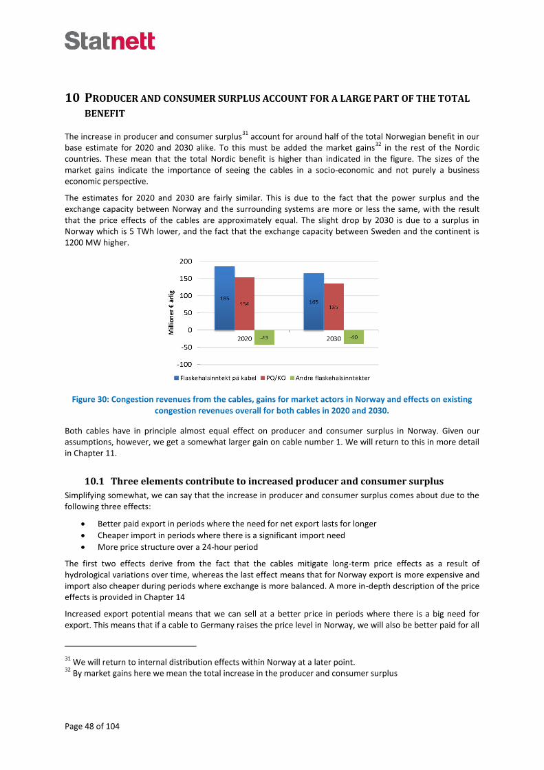
Page 48 of 104
10 PRODUCER AND CONSUMER SURPLUS ACCOUNT FOR A LARGE PART OF THE TOTAL
BENEFIT
The increase in producer and consumer surplus31
account for around half of the total Norwegian benefit in our base estimate for 2020 and 2030 alike. To this must be added the market gains
32 in the rest of the Nordic
countries. These mean that the total Nordic benefit is higher than indicated in the figure. The sizes of the market gains indicate the importance of seeing the cables in a socio-economic and not purely a business economic perspective.
The estimates for 2020 and 2030 are fairly similar. This is due to the fact that the power surplus and the exchange capacity between Norway and the surrounding systems are more or less the same, with the result that the price effects of the cables are approximately equal. The slight drop by 2030 is due to a surplus in Norway which is 5 TWh lower, and the fact that the exchange capacity between Sweden and the continent is 1200 MW higher.
Figure 30: Congestion revenues from the cables, gains for market actors in Norway and effects on existing congestion revenues overall for both cables in 2020 and 2030.
Both cables have in principle almost equal effect on producer and consumer surplus in Norway. Given our assumptions, however, we get a somewhat larger gain on cable number 1. We will return to this in more detail in Chapter 11.
10.1 Three elements contribute to increased producer and consumer surplus
Simplifying somewhat, we can say that the increase in producer and consumer surplus comes about due to the following three effects:
Better paid export in periods where the need for net export lasts for longer
Cheaper import in periods where there is a significant import need
More price structure over a 24-hour period
The first two effects derive from the fact that the cables mitigate long-term price effects as a result of hydrological variations over time, whereas the last effect means that for Norway export is more expensive and import also cheaper during periods where exchange is more balanced. A more in-depth description of the price effects is provided in Chapter 14
Increased export potential means that we can sell at a better price in periods where there is a big need for export. This means that if a cable to Germany raises the price level in Norway, we will also be better paid for all
31 We will return to internal distribution effects within Norway at a later point.
32 By market gains here we mean the total increase in the producer and consumer surplus

Page 49 of 104
the power we sell to our existing trading partners. This gain is particularly linked to periods of high inflows where production from hydropower is at a high level and there is low reservoir storage capacity and unregulated run-of-river power.
On the other hand, increased import potential means that Norway can import a lot more energy in a shorter period than is currently the case. In periods where there is a major energy deficit in the reservoirs, we have a high level of net import from all our trading partners to make up for this. More cables mean that we can trade in this deficit on the power balance at a lower price.
More price structure over the 24-hour period also contributes to the producer/consumer gain. The best way to illustrate this effect is to take as a starting point a period with a balanced net exchange, where the cables do not result in changes to the price level itself. In such situations increased producer and consumer surplus will both contribute to the producer/consumer gain. This is because the hydropower plants utilise their regulating capability by reducing production at night
33, when we can import cheaply, so that they can produce more
during the day. This means that consumers get an additional gain on top of what the producers lose at night when domestic consumption is higher than production, while the situation is the reverse during the day.
10.2 Increasing power surplus and more unregulated production result in greater producer/consumer gain
The three effects explained above mean that we get a big producer/consumer gain irrespective of the assumptions we make about the future power surplus in Norway and the Nordic countries. It is however the case that the gain increases when the imbalances in the power balance in a normal year become greater. Both the Nordic and the Norwegian power balance play a role here. Usually the benefit will increase when these both pull in the same direction. In the base estimates we assumed that the surplus in the Nordic countries will grow from 10 TWh in 2012 to around 30 TWh in 2020 and stabilise at this level. In Norway the surplus will grow from 4 TWh to around 12 TWh in 2020 before dropping back to 7 TWh in 2030. As far as Norway is concerned, there is the additional factor that a lot of the power is unregulated hydropower, whose highest production levels occur when the need to export is already highest in the summer season.
The big gain in the form of increased producer surplus will therefore coincide with the period between weeks 20 and 40, where we get a big proportion of “heavy” production. Of a total of 12 TWh of average export over the year, 80 per cent of this takes place in this period. The graphs in Figure 31 show the prices and total outward exchange from Norway for weeks 23-35, which we define as summer. As we can see, in this period there is on average continuous export from Norway both with and without new cables. On the other hand, cables result in better payment for the export. In addition, we can also see the point relating to movement of export from hours in the night to hours in the day. This results in an additional gain
34.
33 Or in periods with low prices on the continent as a result of a lot of production from renewable sources.
34 Overall, there is slightly more export in these weeks with cables, even if exchange over the years is more or
less unchanged. This is due to the fact that increased export in these summer weeks equates to reduced export in other weeks.

Page 50 of 104
Figure 31: The graph on the left shows the prices in a representative summer week with and without cables in 2020, whereas the graph on the right shows the total outward exchange from Norway in the same period
(weeks 23-25).
In winter, the effect of the cables is slightly different (Figure 32). The cables result in slightly more export during the day from Norway, but power restrictions mean that the effects will be less than during the rest of the year. On the other hand, there is a considerable increase in night-time import. This also results in more price structure over the 24-hour period
Figure 32: The graph on the left shows the prices in a representative winter week with and without cables in 2020, whereas the graph on the right shows the total outward exchange from Norway in the same period
(weeks 49-9).
Overall, the surplus leads to the producer/consumer gain being bigger than the gain we would have had in a more balanced situation. It also means the effect in terms of better paid export will be the dominant one. To illustrate the point about more imbalance increasing producer/consumer gain, but that this would have been big in any case, we will once again compare the case we presented in the previous chapter with the “2020 Balance” case.

Page 51 of 104
Figure 33: Total producer/consumer gain from both cables in the expected 2020 scenario compared to the scenario where both Norway and the Nordic countries are in power balance
Figure 33 compares the total producer/consumer gain from both cables in the balanced dataset with our base estimate. The decrease is around 20 per cent when the balance is reduced by 30 TWh in the Nordic countries and 12 TWh in Norway. Nevertheless, the gain for Norway is still more than EUR 120 million a year. Also, the fact that the cables in this situation contribute increased security of supply has not been fully evaluated.
10.3 Enhanced security of supply
With a Nordic surplus of over 30 TWh, the need for import to the Nordic countries is low even in the driest of years. In addition, the outgoing exchange capacity from the Nordic countries is greater, even without our cables. The gain from cheaper import in dry years is therefore low in our base estimates.
However, there will be greater security of supply. With a 2800 MW increase in exchange capacity, Norway can, if needed, import more in a shorter time and at a lower price than without the cables. We also get a lower probability of no-load operation in the storage reservoirs and rationing in the period just before spring. Such a need may arise if we get a lower surplus and again encounter a period where there are problems with Swedish nuclear power production. As stated, this is not something we have assumed in our main scenario. At the same time, future market trends are unclear and it is not certain that the surplus on the power balance will be maintained. For example, it is not certain what will happen with the Swedish nuclear power plants once their expected lifetime comes to an end around 2030. If we assume that only half of installed power will be reinvested, around 30 TWH of annual production will disappear, i.e. the same as the entire Nordic surplus in our base dataset for 2020 and 2030. Moreover, history has taught us that long-lasting faults can occur on critical transmission power links during dry, cold winters. There is therefore a real possibility that we might also end up in such a situation over the course of the next 20 years.
Figure 34: Prices on average per week over the year in the five driest years in the 2020 balance scenario
with and without cables.
Figure 35: Prices on average per week over the year in the five driest years in the 2020 balance scenario
with outage of 2500 MW of nuclear power, with and without cables.
To illustrate the points relating to cheaper import, we again refer to the scenario where the Nordic countries are in balance. In addition, we have looked at the consequences of having 2500 MW less availability in Nordic nuclear power in the winter period due to an unexpected fault. We provide the results for price in the five driest years in Figure 34 and Figure 35. Without outage of nuclear power, prices go down in the filling season with the cables, due to the increase in import options. The prices after Christmas, on the other hand, remain more or less unchanged. With outage of nuclear power, the effect is, relatively speaking, less in the filling season, but the increased options for import reduce the prices significantly from a nuclear power outage in week 44 and for the rest of the winter and beyond.

Page 52 of 104
The fact that the cables reduce the risk of rationing may be seen as an unpriced gain which should be added to the gain in terms of cheaper import. Our society is entirely dependent on a secure power supply, and a situation involving rationing due to no-load operation in the storage reservoirs will have very serious consequences. Given that there is frequently a considerable risk of rationing in Norway, a lot points to the market not sending the producers price signals which fully reflect society’s willingness to pay to avoid rationing. Both theoretical considerations and empirically based experience indicate that there is a basic disparity between the socio-economic cost of rationing and the “payment” made via the market to avoid it. This suggests that there is additional gain to be had in achieving a lower likelihood of rationing which is not highlighted in our calculations of the socio-economic benefit.
10.4 Sweden benefits significantly from the Norwegian cables
Sweden will benefit significantly from the cables from Norway, as they increase the price level throughout the Nordic countries, so that Sweden too receives better payment for its big net export. We should mention that Sweden does lose a lot of trading revenue on her existing interconnectors. As a result, the Swedish benefit is 25-35 per cent of the total Norwegian benefit. In 2020 the annual Swedish benefit per cable from Norway will be EUR 40-50 million, and in 2030 this increases to EUR 50-60 million. Finland is less affected, but comes off worse, as a higher price level there is not particularly beneficial when they have net import.
Figure 36: Distribution between Norway, Sweden and Finland of the market gains from the two cables in 2020 and 2030
The distribution effects between Norway, Sweden and Finland are determined mainly by the following factors:
1. Congestion both internally in Norway and in the rest of the Nordic countries, particularly between Norway and Sweden
2. The proportion of regulatable hydropower 3. Short-term fluctuations in the power balance due to hydrology and temperature 4. The power balance over time
The degree of internal congestion between the Nordic market areas is one factor which determines now the price effects, and therefore the producer/consumer gain, are distributed to the other Nordic countries. Currently, during most periods the congestion in question is limited, and our other analyses suggest that it will gradually decrease both internally within Norway and between the individual countries, on the basis of the grid development plans currently available
35. This therefore means that, for the market actors in the Nordic
countries, which location/country the cables are built from is fairly unimportant.
Norway has a larger amount of regulatable hydropower than Sweden, and this adds to the Norwegian benefit. In many periods we have day/night exchange with both Sweden and the continent. Norwegian hydropower sells regulating capability to both Sweden and the continent. Currently, with relatively low volatility over a 24-
35 Curves for future price differences internally within Norway are provided in Chapter 3.9

Page 53 of 104
hour period, the market price for this flexibility is relatively low. More price structure over the 24-hour period as a result of the cables means that the price for what we already sell to Sweden (and the other trading partners, Denmark and the Netherlands) will increase.
On the other hand, the power balance will vary over time and be influenced by a number of factors. In our scenarios we have assumed that Norway will have a moderate increase in the power balance compared with today’s, from approximately 5 TWh today to around 10 TWh. Already today Sweden has a surplus of over 10 TWh, which we think will increase to between 20 and 30 TWh. This is very important for the way in which the gains from the cables will be distributed, as Figure 36 illustrates.
Generally it is the case that much of the benefit of the cables will end up in Sweden, because the price level in the Nordic countries will increase. This is very beneficial for Sweden, as they will obtain better payment for their big net export. It is not just the value of the Swedish export to trading partners other than Norway which will rise. Over the year, Norway has a relatively big net import from Sweden, which we export on to Europe. The fact that we have to pay more for this import is a distribution effect which in isolation is beneficial to Sweden and not favourable for Norway.
This also means that the distribution of electricity generation meeting green certificate (“electricity certificate”) requirements between Norway and Sweden affects the distribution of the cable benefit. We made a sensitivity adjustment by moving 4 TWh of wind power from Sweden to Norway in 2020. The result is that around 10 per cent more of the benefit will end up in Norway.
It is also the case that the Norwegian power balance fluctuates a lot more than the Swedish one. This means that the need for export and import between different years can be considerable even if the normal year balance is in reasonable equilibrium. This will also result over time in more of the producer/consumer gain tending to end up in Norway.
10.5 The producer/consumer gain is lower on the continent and in the UK than in the Nordic countries
The way in which the cables affect the prices in the various markets plays a big role in determining the distribution of the market gains between actors in different countries
36. Given that the price effect is clearly
greatest in the Nordic countries, this also means that most of the market gain will accrue to the actors in these countries, a circumstance which is clearly illustrated in Figure 37. Model simulations indicate that approximately 80 per cent of the market gains end up in Norway. In actual fact, the proportion which accrues to Norway and Sweden is slightly higher than the bar graphs below indicate, as Finland ends up slightly in the red.
The big proportion of hydropower in Norway, Sweden and Finland is the main reason why the cables have a greater effect on the price here than in Germany and the UK. In the latter two countries, the price is for the most part set by short-term marginal costs for gas and coal power plants, and a new interconnector to Norway will not have any influence on this which is worth mentioning. Of course, the cables can result in lower price spikes in situations where the grid becomes particularly stretched and there is a low capacity margin. Over time, however, there is reason to believe that the markets will adjust so that the capacity margin remains unaffected by the interconnectors to Norway.
In Norway, Sweden and Finland, for large parts of the time, it is hydropower that sets the price. Nevertheless, water is free, and the water values the producers bid into the spot market are therefore determined by the marginal costs for alternative production internally within the Nordic countries, the risk of flooding and rationing, the potential for exchange with other systems and the price level here. In a situation with a greater degree of unregulated production and a surplus on the power balance, an increase in total exchange capacity of 2800 MW therefore has a clear effect on Nordic prices.
36 The principle here at stake is explained in Chapter 2

Page 54 of 104
Small price effects bring little gain for the market actors on the continent and in the UK. This might appear somewhat strange, given that the overall market here is so large, so one would expect to see a significant volume effect. However, the crucial factor is not the size of consumption and production within a given country, but the net exchange hour for hour with other areas. The rest will just be internal distribution effects between producers and consumers.
Figure 37: Distribution of the market gains between actors in the Nordic countries and the rest of the continent which is modelled in BID, as a result of the cables to Germany and the UK in 2020.
This should not be interpreted to mean that there are no benefit effects for the markets in the UK and on the continent, rather that these are more long-term and/or are not captured in our model simulations. First of all, cables can mean less investments in peak load power plants or make it easier to integrate more wind power. In addition, the cables can help mitigate the highest price spikes experienced by our trading partners in periods where the power balance becomes particularly tight. If a cable can help in cutting something like that, the producer/consumer gain at our trading partners may also be considerable during these periods. This is only captured to a small degree in our model simulations, with the possible consequence that we undervalue the producer/consumer gain in these countries.

Page 55 of 104
11 THE BENEFIT DIMINISHES WITH MORE CABLES
We get diminishing benefit from cables for two reasons: the benefit of smoothing out hydrological imbalances decreases, and we import more price structure over the 24-hour period when transmission capacity increases. Both aspects result in prices which are more similar to those of our European trading partners, so that:
The congestion revenue on our existing interconnectors becomes lower37
Even the congestion revenue and producer/consumer gain from cable number 2 are lower than for cable number 1
Figure 38 shows how the benefit declines with incremental changes in capacity of 1400 MW to the UK. We ran three simulations in the base dataset for 2020 where we incorporated three cables to the UK in succession. Our overall evaluation of these tests indicates that the gain diminishes by 15-20 per cent per cable based on this dataset. However, it should be pointed out that we think that the uncertainty relating to the estimates increases in proportion to increase in capacity. In addition, the exact assumptions we make will affect how rapidly the benefit diminishes. This applies in particular to the power balance in Norway and the Nordic countries.
Figure 38: Diminishing benefit of cables. The figure shows the socio-economic benefit of building three similar cables to the UK based on our 2020 scenario.
11.1 Prices more equal to those in the rest of northern Europe reduce the revenues from existing interconnectors
The red area of the bars in Figure 38, i.e. the producer/consumer gains plus changes to existing congestion, is reduced, mainly as a result of the decline in existing congestion revenues. Gradually, as we get more cables, the effect increases, because the volume on which we lose revenue grows (Figure 39). One of the things we see is that the cable to the UK reduces the revenues on the Germany cable when this comes into service.
37 With Sweden, the case may be different, but the effects in question are still a lot less because the congestion
on the interconnectors is low to begin with.

Page 56 of 104
Figure 39: Decline in existing congestion revenues from the cables in 2020 and 2030 The cable to the UK results in a decline in the congestion revenue to Germany.
The size of the power surplus in Norway and the Nordic countries affects how much we lose on existing interconnectors. More surplus results in higher congestion revenues on existing cables, and therefore also greater decline as a result of new capacity. If, on the other hand, we have a situation where we are in balance, i.e. neither a surplus nor a deficit, the congestion revenues are lower than in our base estimate and the reduction is less as a result of the cables to Germany and the UK. In our alternative dataset for 2020 where there is balance in the Nordic countries, this effect is halved from EUR 45-50 million to EUR 20-25 million per annum, overall for the two cables.
11.2 More equal prices reduce congestion revenue on the cable itself
Greater transmission capacity also results in gradually lower congestion revenues on the cable itself (blue area of the bars in Figure 38). In Table 5 we saw that, in 2020, on average the cable to Germany reduces the price difference to the UK by approximately EUR 2.5/MWh per hour. This reduces the congestion revenues in respect of the UK by approximately EUR 10 million a year.
Most of the reduced price difference is due to the fact that the prices on the Norwegian side become more equal to the prices of our trading partners. At the same time, more cables also result in slightly less price volatility on the thermal side. This makes it somewhat more profitable to build a cable to each country (in our case Germany and the UK) than two to the same country
38. In the longer term, however, adjustments which
are due to the cable, such as less investments in peak load power plants, make the real price effects on the thermal side smaller.
11.3 Favourable distribution effects for Norway result in relatively stable producer/consumer gain
It is generally the case that the marginal producer/consumer gain also decreases as transmission capacity increases. This applies particularly to the first cable we build, as this plays the biggest role in smoothing out price effects in Norway due to hydrology. How much so again depends on the power balance in Norway and the Nordic countries. In our case, the producer/consumer gain is reduced by between EUR 15 and 20 million from the first to the second cable.
However, this effect will be offset by the fact that the price structure over the 24-hour period in which Norway imports will gradually increase as capacity grows. This results in beneficial distribution effects for Norway via the fact that we import more cheaply and sell at a higher price. Thus the marginal decrease in the producer/consumer gain is less.
38 The effect on British prices of a cable from Norway to Germany are minimal.

Page 57 of 104
11.4 Greatest benefit from trading with the UK
In spite of the fact that we incorporate the cable to the UK as number 2, the benefit from this is greatest in 2020 and only marginally lower in 2030. Central factors making trading with the UK more profitable are:
The combination of a big surplus in the Nordic countries and a CO2 price in the UK which is higher than the rest of Europe will result in big differences in the electricity price level
Price volatility is greater in the UK than in Germany. For a given difference in price level, greater volatility on the trading partner’s side results in greater congestion revenue
Figure 40: Total benefit in respect of Germany and the UK in 2020 and 2030 based on both cables being incorporated as the first cable.
Figure 40 compares the benefit from the two cables when we assume that both cables are built as the first cable in 2020 and 2030. It is mainly the congestion revenue which makes a cable to the UK more profitable. We will demonstrate later on that the price effects in Norway of the two cables are of the same order of magnitude. This also means that the effects on the producer/consumer gain and the congestion from other interconnectors will also be more or less equal.
The benefit is reduced if the CO2 component in EMR disappears.
In our base estimates we gave a weighting to different CO2 price scenarios in the UK due to the great uncertainties relating to this additional surcharge, which is planned as part of the major British energy market reform. Here we show results from simulations where the British remove the CO2 component, but otherwise retain unchanged the other aspects making up the reform. The simulations have been performed with a 2020 dataset.
Figure 41: Effects of the CO2 component not being part of the British energy market reform in 2020.
We can see that the total benefit is reduced by EUR 15 million per annum, representing a decrease of 10 per cent. The reduction in congestion revenue is greatest in absolute terms, at EUR 10 million. The reduction in the socio-economic increment is around half of that, but just as great in percentage terms. The reason why the benefit decreases is that electricity prices in the UK are reduced by EUR 3/MWh.

Page 58 of 104
12 FLUCTUATIONS IN WEATHER AND FUEL PRICES INCREASE THE EXPECTED BENEFIT
AND RESULT IN A BIG ANNUAL VARIATION
Natural fluctuations in weather39
and economic cycles, together with unexpected events40
, will result in big annual variations in the cable benefit. Correlations between these factors which affect cable benefit in the same direction reinforce the effects at certain periods, while the opposite can also be the case. This results in a good deal of uncertainty relating to the benefit from year to year, but overall it tends to exert upward pressure on the average benefit we calculate in our estimates.
12.1 Variation in inflow increase congestion revenues and producer/consumer gain
Variation in the inflow on the Norwegian and Nordic side is the factor which, in Norwegian eyes, most definitely is of greatest significance in terms of the benefit to be derived from the cable. This applies to both the level we assume in our estimates and to annual variation. Temperature-dependent consumption reinforces the effects of variations in inflow, as there is a positive correlation between the two. These variations contribute positively to the anticipated benefit.
The fluctuations are important both for the congestion revenues and the producer/consumer gain. The figure below shows how the three components and the total benefit, for both cables, vary over the 47 years we are simulating. The figures are taken from the 2020 estimate. All lines are sorted by magnitude of total benefit.
The big variation is due almost exclusively to hydrology, although the wind on the continent can be a source of considerable “noise”. The future power surplus in Norway and the Nordic countries means that it is mainly wet years which result in benefit higher than the average. Years which are drier than normal result in lower benefit, as the price level in the summer season in those cases is more like the price level generally in northern Europe. It is also the case that, due to the big surplus we have in a normal year, a wet year will increase the benefit more than a dry year reduces it.
Figure 42 The sum of the various components for both cables in 2020 per inflow year. All years are sorted by magnitude of total benefit. Spelling mistake in figure.
The producer/consumer gain is the component which fluctuates greatest, from approximately EUR 600 million a year to around zero. The greatest gain is in wet years when the price effects of the cables are greatest, and net export is high. In years where the cables exert upward pressure on electricity prices, because Norway, Sweden and Finland as a whole have a surplus, the producer/consumer gain can, on the other hand, be very
39 Inflow, temperature, wind and sun.
40 Outage of power plants and transmission power links

Page 59 of 104
low, because the power we import gets more expensive. The median value for producer/consumer gain is around EUR 100 million, whereas the average is over EUR 150 million.
The congestion revenues vary from EUR 100 million to over EUR 300 million. The average is approximately EUR 10 million higher than the median value. The variations tend therefore to push the estimate upwards, but less so compared to the producer/consumer gain. Variations in wind power on the continent are also a source of “noise” and can explain differences in congestion revenue between relatively similar hydrological years.
There is a positive correlation between the congestion revenues and the producer/consumer gain in spite of the fact that in isolation major price impacts result in lower congestion revenue. This is due to the circumstance that although the price impacts are highest in years with most inflow, they are not big enough to prevent the Norwegian price level being significantly lower than that on the continent over large parts of the year. This means that both the congestion revenues and the producer/consumer gain will be big in these years.
There is a negative correlation between the congestion revenues from other cables and the producer/consumer gain, but this component plays a minor role compared to the other two. Overall there is a very significant variation in total benefit, ranging from EUR 150 million up to EUR 800 million a year.
12.2 Wind power on the continent results in big annual variation in the congestion revenues
When it comes to climactic conditions on the British and German side, it is variations in wind power production which have the greatest importance for year-on-year changes in the benefit derived from the cables. This affects the congestion revenues, but producer and consumer surplus in Norway only to a lesser degree.
We have eight different wind years in our simulations. The figure shows the congestion revenue in respect of Germany in the various years compared to what we have defined as a “normal” wind year. The Norwegian share of the congestion revenue varies by around EUR 90 million between the different years for the Germany cable.
Figure 43 Different wind years compared with a normal wind year. Negative congestion revenues occur on the basis of this comparison, but will not occur in real life.
We can see that there is a positive correlation between the congestion revenues and the amount of wind power production on the continent/in the UK. The observation on the extreme right of the figure shows that this is not necessarily the case, but the trend does point in this direction. The reason why high wind power production results in high congestion revenue is that it leads to more zero prices in winter on the German and British side. We have made a careful calculation and arrived at the conclusion that congestion revenue increases by approximately EUR 4 million when wind power production increases by 1 TWh in Germany. We have too few historical wind years in our model to be able to hazard an exact statement as to how strong the relationship is.

Page 60 of 104
Although there is a clear relationship between the amount of wind power within a year and the congestion revenues, any conjecture as to how much the variations raise the average compared with a “normal” wind year is more problematic. In our simulations, the average for the eight years is approximately EUR 3 million more than a normal year. Whatever the case, more wind years result in a more unbiased and robust estimate.
12.3 Solar power is more predictable than wind power
German solar power has a period of use of only around 900 hours in the year. On the other hand, this is concentrated in hours of the day where consumption is highest and the need for power greatest. The contribution can also vary greatly over large parts of the year. Production grows rapidly from the start of March, before dropping off in October and beyond. Variation within different 24-hour periods in this overall period can be considerable. There is therefore a negative seasonal correlation with wind power, most of which is produced in the winter months.
Figure 44: Production over 24-hour period for a summer day on the left and a winter day on the right. Solar power covers a lot of the consumption in summer.
We only have historical data for one year’s solar power production in our model. This makes it difficult to say anything specific about the annual variation in benefit as a result of different sun years. New sun series are under preparation, and preliminary results indicated that solar power production has a lot less variation in production from year to year than wind power. This means that the annual variation in benefit will also be low, although the variation between 24-hour periods may be considerable over shorter periods.
12.4 Economic cycles and fuel prices
Fluctuation in economic cycles affect the electricity demand and the prices of coal, gas and CO2. This may therefore have considerable importance for cable benefit.
We are basing our assumptions about the coal and gas prices on the IEA’s New Policies Scenario. In addition, we have an annual seasonal profile for gas designed to represent storage costs. The prices represent a state of equilibrium, but history shows that the prices can deviate from this at certain periods. We have therefore provided a weighting for short-term variations in fuel and CO2 prices in the base estimate based on sensitivity analyses and historical price variation. This relates to changes in the actual price level and the relative state of marginal costs in coal and gas power plants. The changes we have made are conservative with the result that we do not cover the entire sample space. Overall these variations lift the estimate by around 3-8 per cent.
Fluctuations in demand for electricity can have a somewhat different effect in the Nordic countries and in Europe. On the continent the impact on the electricity price is mainly due to changes in capacity margins in peak hours. Lower power consumption, which results in lower peak prices and congestion revenue, can however be offset to some extent by more zero prices in off-peak electricity. Nevertheless, it is very difficult to quantify such effects, and we have opted not to provide a weighting for this in the base estimate itself. Instead, the effects are included in the estimates which are intended to cover the sample space.

Page 61 of 104
In the Nordic countries, economic downturns will result in lower power consumption and therefore greater surplus, as production is not particularly price-sensitive in the shorter term. This means that it is maintained even if consumption decreases. In isolation, this will push cable benefit upwards. Reduced consumption in the Nordic countries therefore has the opposite effect on the benefit from cables.
Overall we think that the benefit will be greatest in typical economic recoveries where fuel and CO2 prices are relatively high and there is a big demand for electricity. In downturns, the benefit will decline, but this can be to some extent offset by the fact that the power surplus in the Nordic countries increases.

Page 62 of 104
Part III PRICE AND DISTRIBUTION EFFECTS
The cables to Germany and the UK affect the prices in Norway and the Nordic countries in various ways. We have more stable prices throughout the year, but also more short-term price volatility. Since we expect a greater power surplus and more unregulated production, taken in isolation, the cables will also result in a higher price level in Norway. Long-term market adjustments may however mitigate this effect somewhat.
Price effects on the Norwegian side mean that a large part of the benefit will be in the form of increased producer and consumer surplus. At the same time, this results in distribution effects between producers and consumers.
In this part, we first take a look at how the cables impact on prices on the Norwegian side, before examining the distribution effects between producers and consumers. This should not be interpreted as a set of exact prognoses either for future price trends in Norway or for distribution effects between producers and consumers.

Page 63 of 104
13 THE CABLES ARE ONE OF SEVERAL FACTORS WHICH AFFECT ELECTRICITY PRICES IN
NORWAY
Already today, the average electricity price in Norway is closely linked with the European level. The prices for coal, gas and CO2 are therefore important drivers behind Norwegian prices and will probably continue so for the next 20-30 years, irrespective of whether we build cables to Germany and the UK. Other central factors for the future evolution of the Norwegian average price is the combined power balance in Norway, Sweden and Finland, and the total outward exchange capacity from the Nordic region.
Figure 45: Simulated average prices in southern Norway over 47 inflow years for 2012 and the base scenarios for 2020 and 2030 (with both cables included).
The level of fuel and CO2 prices determines the short-term operating costs of thermal power plants and is the single factor which has the greatest bearing on the future price level
41 in Norway and the Nordic countries.
Given our base assumptions about future fuel and CO2 prices (shown in Figure 9, Chapter 3.6), we get a gradual increase in electricity prices throughout Europe between now and 2030. This applies in Norway as well, as Figure 46 shows. Increasing prices for CO2, from EUR 7/tonne in 2012 to EUR 22 and EUR 45/tonne in 2020 and 2030, respectively, are of particular importance. Taken in isolation and using the 2012 dataset as a basis, the price effect of this is an increase of EUR 12/MWh by 2020 and EUR 27/MWh by 2030.
There is a great deal of uncertainty as to future CO2 prices and the role of the quota market as a climate policy instrument (discussed in more detail in Chapter 18). The quota prices may therefore be both higher and lower than the levels we have assumed in our base dataset for 2020 and 2030. However, this does not alter the main point in this context: that the marginal costs for thermal power plants are crucial to the Norwegian price level, in spite of the fact that Norway has almost no thermal power plants.
After fuel prices, it is the ratio of the surplus on the Nordic power balance to the total transmission capacity between the Nordic countries and the surrounding systems which is the most important factor for the Norwegian price level. The greater the surplus and the lower the transmission capacity, the lower the price level in Norway and the Nordic countries relative to that in Europe. We should here point out that the Norwegian power balance per se is of secondary importance, except for the manner in which it affects the total Nordic balance.
The phasing in of 45 TWh of new renewables and nuclear power between now and 2020 will result in strong downward pressure on prices in Norway, Sweden and Finland. In isolation, growth of this type results in very low prices relative to the rest of north-west Europe, with prices tending to zero during many periods. However, we are of the opinion that growth in consumption and the phasing out of fossil fuel production in Finland and Denmark will manage to contain some of the growth in production, so that the Nordic countries will have a surplus of around 30 TWh in a normal year around 2020. Moreover, with the cable power link currently under construction
42, plus the transition to flexible trading between Finland and Russia, the downward pressure on
41 By price level we mean the average price over the year. When we refer to a simulated future price level, this
is, in addition, an average over 47 historical inflow years. 42
Estlink 2, Norbalt, SK4 and more capacity between Denmark and Germany.

Page 64 of 104
prices will be a lot less than had we incorporated 45 TWh of new production and otherwise kept everything else the same. Simulating with our base assumptions, we therefore obtain a reduction in price between now and 2020 which is moderate in comparison to today’s levels, provided we hive off the combined effect of increased surplus and greater transmission capacity beyond what we get with the cables to Germany and the UK. If, on the other hand, the surplus were to be higher than our assumptions indicate, then prices will soon become considerably lower.

Page 65 of 104
14 THE DIRECT PRICE EFFECTS ARE A HIGHER PRICE LEVEL, GREATER STABILITY OVER
THE YEAR AND AN INCREASE IN 24-HOUR VARIATION
By direct price effects we mean changes in Norwegian and Nordic prices as a result of the cables compared with a situation where there are no cables but otherwise identical generating portfolio, demand and exchange capacity. As we explained in Chapter 5.4, these are the same price effects which result in the various elements in the socio-economic balance sheet in our base estimates.
14.1 The price level increases, but is still lower than in Germany and the UK
The cables to Germany and the UK will result in a higher price level in Norway and the Nordic countries. With the specific assumptions we have used in our base estimates, our simulations indicate that the average price in Norway will rise by EUR 4.9/MWh (NOK 0.039/kWh) in 2020 and EUR 4/MWh (NOK 0.032/kWh) in 2030. This is the effect in isolation of both cables combined. It is far from certain, however, just how big this effect will actually be. If we get a lower Nordic surplus than we have assumed and greater transmission capacity to other systems, the prices will increase less. If, on the other hand, there is a trend in the opposite direction, the increase will be greater. In addition, the market can adjust to what is in relative terms a low price level if the cables were not to be built. This will reduce the cables’ real effect on the price level, and is discussed in Chapter 15.
A surplus on the power balance and more unregulated production, both in Norway and the Nordic countries overall, is the main reason we get a higher price level with the cables. From the outset, this exerts downward pressure on the Nordic price level. The growth resulting from the cables will therefore be from a relatively low level and should accordingly be seen in this light.
A point that we will return to in the next sections is that it is mainly wet years which push up the average. The increase in price we get with the cables is therefore not due to even price growth alone, but is also a consequence of more even prices over the year and between wet and dry years.
Another important point is that the price effect in Norway for a cable to the UK is almost the same as with Germany, even though the price level is higher in the UK. This is due mainly to the fact that Norway does not import the prices of the trading partner directly. The price change is a reflection of how the cables effect the net exchange between all countries with which we trade. The effect is more or less the same, even if the price level in the two countries is different in our base scenarios. On the other hand, if the power balance margins in the Nordic countries become tighter, the conclusion we draw here will change accordingly. The price level in the country to which we build a cable will then have a greater effect on the price level in the Nordic countries.
The fact that the two cables have more or less the same effect on the price level is also due to the interconnector with the UK being number 2. If this interconnector had gone to Germany as well, the price effect and the gain from trading would both have been slightly lower than for the other cable.
In spite of the fact that we get slightly higher average prices with the cables, these will still be below the average prices at our trading partners. In our base dataset for 2020, the price in Norway, where both cables are included, is on average approximately EUR 5.6 and EUR 14/MWh below the level for Germany and the UK, respectively.
14.2 Prices become more stable over the year – the effect is greatest in summer
The price effects in the Nordic system will vary over the year and from year to year depending on hydrological conditions. Our simulations indicate that the effect is greatest in summer and least in autumn, as Figure 49 shows. The fact that the prices increase slightly more in summer is due to the export need being at its greatest in this period, with a lot of unregulated production which has to be found a way out of the system. More small-scale hydropower generation adds to this further. The water values, however, serve to spread the effect over the year as a whole. The result is that prices will also be higher in winter, even though net exchange in this period is almost unchanged.

Page 66 of 104
Figure 46: Average prices per week over 47 inflow years in Norway with and without cables in 2020.
Figure 47: Duration curve for all hourly prices over 47 simulated inflow years
43
Figure 47 illustrates the point that prices rise most in periods where the price is lowest at the outset. The curve with the cables is flatter than the one without them because the price differences between different hydrological periods become smaller. In these periods, the cables result in export being relocated to hours where we get a better price from our trading partners, resulting in higher prices on the Norwegian side. A reduced risk of water wastage in the wettest periods also helps raise the price level, as this has an impact on water values for regulated hydropower.
Figure 48: Simulated average prices per week in southern Norway for 10 typical normal years, with and without cables
In typical normal years we see that prices increase reasonably evenly over the year, apart from in autumn, when the prices change less (Figure 48). On average, prices in these years increase by around EUR 3.8/MWh towards an average of approximately EUR 5/MWh over all simulated inflow alternatives.
14.3 Prices become more stable from year to year, even if inflow varies
The effects of the cables in different hydrological years naturally reflects the big surplus in a normal situation. From the graph in Figure 49, which shows the average price per inflow year, we can see that prices increase in all years apart from the very driest, but that the effect is clearly greatest in those years where the price is lowest. The fact the prices increase marginally even in the driest years is due to the big power surplus. Unexpected events may however alter this. If problems were to occur in Swedish nuclear power in a dry year (an occurrence we have observed in recent years), the cables might also result in lower prices, even with a big power surplus in a normal year.
43 A total of 138,684 prices

Page 67 of 104
Figure 49: Duration curve for the average price per year over 47 inflow years, in 2020
Figure 50: Average price per week over the year in the 5 driest and 5 wettest years that we simulate, in
2020
The graph in Figure 50 shows the average prices per week over the year in the five wettest and driest years with and without cables. In the driest years, the effect of the cables on prices is small. The reason that they increase slightly in winter is that there is not enough production capacity to cover both consumption and full export. This means that we often import the price of one of our trading partners during the day.
In the wettest years, prices rise throughout the entire year, but obviously rise most in the summer months when a large proportion of unregulated production has to be drained off.
14.4 When there is a low power surplus, the cables have less of an effect on the average price level
To illustrate the fact that the price effects depend on the power balance, we have constructed a dataset based on 2020 but where both Norway and the Nordic countries are in balance, whereas the prices on the continent remain unchanged. In comparison to our base dataset, here we have incorporated more industrial consumption in Norway and reduced nuclear power production in Sweden.
The figures below illustrate the price effects of the cables in this sensitivity. The figure on the left shows the average price per year in sequence for all 47 simulated years, whereas the figure on the right shows the years sorted by magnitude. As we can see, we now get periods where the cables increase and reduce the prices. At the same time, the effect on average prices is slight in most years. The main reason for the cables still resulting in a somewhat higher price level over 47 inflow years is that the price effects in wet and dry periods are asymmetrical. There is a very clear tendency for prices to fall in wet years by more than they rise in dry years.
However, cables have the consequence that the electricity market finds itself less exposed to unforeseen events, such as outage of the remaining nuclear power units. In reality, really big price impacts often occur when we have a dry year combined with such events. There is therefore reason to believe that the simulation results underestimate the real price effect of cables, as our models do not capture events of this type. This is of course more relevant in a scenario where there is power balance rather than a big surplus.
When such situations occur, the cables also entail a security of supply aspect, and the full value of this will not be captured by the prices. This contributes to the fact that the model underestimates the value of dry year backup.

Page 68 of 104
Figure 51: Average prices per simulated inflow year, shown in sequence from 1962 to 2008, in the
hypothetical scenario where Norway and the Nordic countries are in power balance in 2020.
Figure 52: The same price as those in the figure on the left, but sorted here on the basis of high to low
average annual price.
With tighter margins to the power balance, the effects on price level of a cable to Germany and the UK will be different. The cable to Germany will increase the average level in Norway by approximately EUR 0.75/MWh, whereas the cable to the UK will increase the level by approximately EUR 1.5/MWh. This is due to the fact that the price level at the trading partner will have a greater impact on Norway if the power balance margins in the Nordic countries are tighter.
14.5 The cables result in greater 24-hour variation in prices
The large proportion of regulated hydropower results in significantly lower price volatility in Norway, Sweden and Finland than is the case in the UK and on the continent. As we explained in Chapter 4.2, however, the current hydropower system is not able to achieve even distribution of all price variations, and that is why we already today have periods of variation in prices, typically between day and night.
Although there is still a lot of potential for redeploying production from regulated hydropower, there are many restrictions on how much of the production can be relocated. With more cables we will encounter these restrictions more of the time, and we get:
More frequent output restrictions in winter
Greater variation between the water values in each individual reservoir
More hours involving almost a full break in regulated production in summer
Gradually this results in more short-term price volatility on the Norwegian side, as Figure 53 shows. Here we have taken the difference between the price hour for hour and the average price for the 24-hour period in question. Then we have taken the average of this again, so that we again end up with a value per 24-hour period. Finally we have calculated the average of this value over longer periods, such as spring, summer, autumn and winter. Overall, this gives an indication of short-term price volatility in the form of average 24-hour variation.
The black line shows the historical average over the year based on the prices in southern Norway for the last 10 years, whereas the blue bars show the simulated average per season with and without cables in 2020.

Page 69 of 104
Figure 53: Price volatility over 24 hours in Norway per season with and without cables in 2020. The black line shows the average price volatility over 24 hours for the entire year, based on prices from 2002 to 2012.
First we see that volatility has historically been somewhat higher than the value in our simulations for 2020 without cables. The main reason for this is that the model has a simplified water value calculation so that the supply curve in the model is flatter than the real curve
44. In addition the model also underestimates how often
output restrictions will occur and the effect of exogenous shocks.
One of the reasons we get increased price variation as a result of the new cables is simply that the supply curve is currently not completely flat. This means that, in periods of export by day and import by night, with the cables there will be a greater difference in the water values which determine prices
45. This effect will only be
reproduced to some extent in our model simulations as we have here a flatter supply curve than the one we use as our starting point. We also believe that we get greater differences in the water values between reservoirs with different characteristics if we have more cables, so that the supply curve becomes steeper. Simplifications in modelling hydropower mean, however, that this effect tends not to be captured in our model simulations.
Although our model simulations underestimate these two effects, we can see in Figure 53 that volatility over a 24-hour period increases with cables and becomes higher than we have observed historically during the last 20 years. Volatility increases in all seasons, but most of all in winter and autumn.
In winter it is mainly power shortages which result in price structure over a 24-hour period. This occurs when output in Norway/the Nordic countries is not sufficient to both satisfy high domestic consumption and ensure export to all countries with a thermal price structure. The cables will increase the number of cases with this type of power shortage and therefore result in more hours where we see the Norwegian price at the level of the peak price of our trading partners. There is also a strong correlation between this effect and the power balance. When we used a Nordic balance with tight margins in our simulation, the time when we “import” continental prices increases considerably due to power shortages in winter.
In the period from the spring thaw until inflow declines in autumn, we get more hours involving almost a full break in regulated production. This can result in situations where the price is set by the water values of the hydropower plants during the day, but falls to levels determined by import or unregulated production at night. Our model results indicate, however, that this effect is moderate, as in most cases there is continuous export in spring and summer. In autumn, on the other hand, we see that this contributes to increased price volatility in Norway.
44 We will return to this in Chapter 19.2
45 The demand curve shifts 2800 MW to the right in hours of full export, whereas in hours of full import the
supply curve shifts 2800 MW to the right.

Page 70 of 104
15 LONG-TERM MARKET ADJUSTMENTS CAN REDUCE THE PRICE EFFECTS
In the previous chapter we saw that the cables in isolation result in a somewhat higher price level in Norway/the Nordic countries, and that this is mainly due to our assumptions about a greater power surplus and more unregulated production in Norway and the Nordic countries. If the cables are not built, however, as we discussed in Chapter 5.4, it is possible that the market will adjust to the price level, which, relatively speaking, will be low. This can happen in that we either get more new cable power links from Sweden to the continent, or we on the Norwegian side get increased growth in consumption and lower growth in production. If this happens, we get a higher price level without the cables as well, and the real difference in the Norwegian price level with and without the two cables is thereby reduced.
We see it as a distinct possibility that we would get some kind of adjustment if our projects were to be shelved, but the response will probably not be big enough to result in the same price level with and without the cables. For this reason, we have opted to analyse the effect of long-term market adjustments by incorporating an increase of just under 6 TWh (620 MW) in industrial consumption in our reference case simulation for 2020. This is half the net export we get on the two cables. We have located the consumption in Norway, but the effects would be similar if the consumption were located in Sweden or Finland. On the other hand, the effects would have been slightly different had we chosen a different type of consumption with a different consumption profile.
The graph in Figure 54 shows the average price per week over the year, where the price on average is EUR 3/MWh (NOK 0.024/kWh) higher with cables than with more industrial consumption. This is due mainly to higher prices in summer, as cables contribute more to draining off the surplus than does industrial growth. From around week 35 to the end of the year, the prices are more or less the same. After Christmas, on the other hand, the prices become slightly higher with cables due to more capacity charge elements. That is to say, there is not enough production capacity on the Norwegian/Nordic side to satisfy consumption and provide full export at the same time. In such a case, the price rises for a short time to the continental price level to ensure less export. The reason we have more capacity charges with the cables is that these, on export, increase demand by 2800 MW, whereas industrial consumption only results in an increase just above 600 MW
46.
Figure 54: Average prices over 47 inflow years per week in 2020 for three alternatives: With cables,
without cables, and without cables but with 6 TWh of industrial growth.
Figure 55 Duration curve over hourly prices for all simulated inflow years.
To illustrate more clearly the effects in wet and dry years/periods, Figure 56 shows the average price per week in the five driest and wettest years in our inflow series. Overall the prices are similar in the five driest years, whereas they are around EUR 7.5/MWh higher in the wettest, in 2020. In dry years the prices are somewhat
46 Equates to 5.5 TWh of flat industrial consumption

Page 71 of 104
lower in the filling season. This is due to the fact that Norway, with a higher transmission capacity, can import more cheaply, and that there is less need for major savings. On the other hand, prices increase in winter due to more capacity charges from import.
Figure 56: The average price per week over the year in the five driest and wettest years with cables or industrial growth, respectively.
In the five wettest years, we see that, to a somewhat greater degree, the cables prevent very low prices in periods with a lot of unregulated production. Again, this is due to consumption raising demand by approximately 620 MW, whereas for a lot of the time two cables result in five times as much output capacity.
The fact that short-term price volatility will differ with and without cables can also result in adjustments, but these will take a slightly different form. Greater price volatility increases profitability for investments in more output or pumps in the hydropower system. This can to some extent mitigate import of more price structure over a 24-hour period.

Page 72 of 104
16 PRODUCERS EARN MORE ON AVERAGE, AND CONSUMERS GET BETTER SECURITY OF
SUPPLY
The increase in the overall producer and consumer surplus also involves redistribution between the two groups. Which way the distribution goes is closely linked to the price effects we discussed in Chapters 14 and 15, and the large volume of annual production and consumption in Norway means that even small changes in price level result in noticeable distribution effects when we look at the country as a whole.
As far as future market trends can currently be identified, the cables are most likely to result in redistribution from consumers to producers in the period up until 2030. Nevertheless, the extent of this redistribution is not clear, as it depends on future trends in the power balance, the growth in exchange capacity between the Nordic countries and other systems, and the size of potential market adjustments if we do not build the cables. Who enjoys a net gain will probably vary throughout the cables’ long lifetime, due both to changes in market conditions and as a result of hydrological fluctuations.
16.1 The distribution effects should be seen in a wider context
It makes sense to see the distribution effects we obtain as a result of the cables in the context of the expansion in production from renewable sources. In several of the preceding chapters we have discussed how expansion of production from renewable sources, in combination with more nuclear power in Finland, exerts downward pressure on prices, to the advantage of consumers. Certainly, the construction of other cable power links, reduced thermal production, growth in consumption and flexible trading with Russia will, along with other factors, mitigate the drop in price (cf. the discussion in Chapter 13), but it is not clear by how much. It is therefore likely that, as a consequence of the expansion in Norway of electricity generation meeting green certificate (“electricity certificate”) requirements, consumers will stand to gain in the form of lower average prices before we build cables to Germany and the UK.
47 Looking at production from renewable sources and
cables as a whole, this reduces the redistribution from consumers to producers. Also, irrespective of the other market trends in the Nordic region, it may well result in consumers enjoying a net gain overall.
When we discuss distribution effects, it is important to include in that discussion the full value of increased security of supply. Although an increasing power surplus initially reduces the cables’ role in ensuring energy accessibility, there is a consumer gain in the form of reduced likelihood of rationing, a factor which is not assigned its full value in our simulations, cf. the discussion in Chapter 10.3.
The fact that the cables result in higher electricity prices will also lead to a reduction in the certificate price. By how much is difficult to say, but it would be reasonable to expect that the certificate price will on average be reduced more or less in proportion to the increase in electricity price. This means that any actor who has an obligation under the electricity certificate system must pay less for consumption which is related to that obligation. This should also have a bearing on the discussion about distribution effects.
16.2 There will be big direct distribution effects as a result of an increase in price level
Figure 57 shows the direct distribution effects of the cables in 2020 using our base assumptions. Overall, the increase in price level results in a redistribution of around EUR 600 million on average from consumers to producers per year. In our base dataset for 2030, we also have a big surplus on the Nordic power balance. This results in a redistribution of around EUR 550 million from consumers to producers. Nevertheless, as mentioned above, the distribution effects should be seen in the context of the expansion in production from renewable sources and general market trends in the Norwegian system.
47 We leave changes in fuels and CO2 prices out of the comparison for the moment

Page 73 of 104
Given that it is uncertain how big the effect on the price level will be, the impact of the distribution effect of the cables in isolation may be both greater and smaller than we show here. The question also remains open as to how far into the future redistribution along these lines will continue. A point we intend to return to in the next sections is that the distribution effects will change if there is less surplus, more cable power links and/or long-term market adjustments.
The duration curve in the figure on the right shows the distribution effects for each simulated year sorted by size of increase in producer surplus. As we can see, the distribution effects are of course greatest in wet years when there is the biggest increase in electricity price.
Figure 57: Direct distribution effects between producers and consumers internally in Norway in our base dataset for 2020. The figure on the right shows the effects for all of the 47 simulated inflow years in 2020
sorted by extent of Producer gain.
Redistribution from consumers to producers is not just driven by greater power surplus and a greater amount of unregulated production. More 24-hour variation in the prices also results in distribution effects in favour of producers, although consumers profit by lower net prices.
16.3 Tighter power balance margins result in smaller distribution effects
In the alternative scenario we presented earlier, in which both Norway and the Nordic countries are in power balance, the direct distribution effects will be smaller. Redistribution from consumers to producers is reduced on average per year from more than EUR 600 million to below EUR 300 million. However, the fact that there are distribution effects in favour of producers is due to the asymmetrical price effects in wet and dry years/periods and the high price level in the UK relative to the rest of our trading partners. In addition, we get increased price structure in Norway in the same way as we did in the base dataset – something that producers profit from.
When Norway and the Nordic countries are in power balance, the risk of energy shortages in dry years increases. The cables then play a greater role, by improving security of supply via dry year backup. This value is not fully captured in our model simulations.

Page 74 of 104
Figure 58: Distribution effects between producers and consumers internally in Norway in 2030 in a hypothetical scenario where both Norway and the Nordic countries are in power balance. The figure on the
right shows the effects for all of the 47 simulated inflow years.
With the cables, the power generation system is less exposed to critical evens in dry years, such as outage of nuclear power units. If such an event occurs, consumers will profit more in a dry year than the model simulations directly indicate, and the value of dry year backup increases. Figure 59 shows a case where we have assumed outage of 2500 MW of Swedish nuclear power in a scenario where the Nordic countries are in power balance in a normal year. For the purposes of comparison, in winter 2009/2010 production was on average 3500 MW lower than normal in this period.
Figure 59: Distribution effects between producers and consumers internally in Norway in 2030 in a hypothetical scenario where both Norway and the Nordic countries are in power balance and there is a 2500
MW outage in nuclear power. The figure on the right shows the effects for all of the 47 simulated inflow years.
Here too there is on average a slight transfer from consumers to producers. We can however see that in the driest years there is a substantial gain for consumers, with total savings of up to EUR 1,000-2,000 million a year. It is important to emphasise that this is not due to extreme prices in the very driest periods where areas run short of water, but a generally lower price level (see Figure 35).
In addition to this, consumers gain, in that the cables reduce the likelihood of rationing, as discussed in Chapter 10.3. This is an unpriced gain which is additional to the gain in terms of cheaper import.
16.4 In the event of a power deficit, there is a net gain for consumers
The new cable power links have an economic lifetime of 40 years, so they will be in service up until 2060. Over such a long time perspective, the power balance in Norway and the Nordic countries can fluctuate considerably. Even if there appears to be little risk of developing a greater power deficit over the next 10-20 years, this may well happen over the course of the cables’ economic lifetime. For example, given the power plants’ lifetimes, all existing nuclear power in the Nordic countries is due to be phased out between 2025 and 2040. Though we do not believe it to be the case, it is possible that some of the reactors will not be replaced.
Here we have illustrated the potential distribution effects where there is a 12 TWh deficit on the Nordic power balance, with half of that being in Norway (-6 TWh). This is based on a number of factors: expansion of production from renewable sources will come to an end in Norway after 2020; some of the nuclear power in Sweden will be decommissioned at end of lifetime; there may be less of a decline in general supply
48 and more
consumption from server farms. We have also removed the additional CO2 component in EMR in the UK.
48 In our base dataset we have a decline in general supply in Norway and Sweden due to energy efficiencies

Page 75 of 104
Figure 60: Distribution effects between producers and consumers internally in Norway in 2030 in a hypothetical scenario where both Norway and the Nordic countries are in deficit on the power balance. The
figure on the right shows the effects for all of the 47 simulated inflow years.
In this case, both consumers and producers profit on average from the cables. The gain in question is of the order of approximately EUR 90 million for the producers and around half that for consumers. If the deficit were to be even greater, redistribution from producers to consumers would increase significantly.
16.5 Long-term adjustments result in smaller distribution effects
In Chapter 15, we showed how long-term market adjustments can reduce the difference in price level with and without the cables. To illustrate how this affects the distribution between producers and consumers, we again take as starting point our reference case where consumption response is just under 6 TWh. Due to smaller price effects, the distribution effects from consumers to producers will also be reduced by approximately 40 per cent compared to a case without consumption response. The actual gain which the producers enjoy over and above what the consumers lose is reduced by about 15 per cent. Much of the redistribution, and the gain, occurs in the 10 wettest years. In most years redistribution is small.
Figure 61: Distribution effects of cables if we compare the scenario with cables to an alternative development scenario where more industry is established
Given that the establishment of power-intensive industry drives the price level up, this also results in big distribution effects. In the case we have looked at here, with industrial establishment consuming 620 MW on an even basis, this costs existing Norwegian consumption around EUR 250 million per year.

Page 76 of 104
Part IV UNCERTAINTY AND SAMPLE SPACE
There are several forms of uncertainty associated with the benefit of the cables. Here we look at what we consider the most central aspects in each category, before going on to discuss the implications these have for the sample space. Finally, from an overall perspective we discuss the robustness of estimates and sample space in the light of all of our work on the analysis.

Page 77 of 104
17 METHODS FOR DEALING WITH UNCERTAINTY
Building cables to Germany and the UK will mean some big investments. It is therefore important that we have a good idea of the uncertainty involved in estimating the benefit. A central part of our work on the analysis has therefore been about achieving an understanding of the most important areas of uncertainty and how these affect the benefit. Here we give a brief outline of our work on this.
17.1 We see several types of uncertainty
At a general level, we can analyse the uncertainty relating to future cable benefit into the following three categories:
Scenario uncertainty
Weaknesses in model, method and data basis
Annual variation in benefit due to fluctuations in weather, fuel prices and similar factors
All three contribute to the overall uncertainty of our estimates of future gain from trading in different ways. For the decision whether to build the cables or not, we do however think that scenario uncertainty is the most important. In our work on the analysis, we have focused therefore mainly on this category.
Although we have spent a lot of time analysing uncertainty, it is important to point out that there are likely still to be areas of uncertainty which we have not as yet identified or fully understood. Nor perhaps is it possible to achieve such full understanding, but we can indicate various factor which might be of potential significance.
17.2 Two-stage identification of scenario uncertainty
Scenario uncertainty is the sum of all uncertain aspects pertaining to the future development of the power generation systems which also are of significance for cable benefit. We have therefore approached this in two stages:
Identifying areas of uncertainty in the future development of the power generation system in all of north-west Europe
Analysing how those factors which are uncertain affect cable benefit
It is only once we combine these that we get an idea of scenario uncertainty. The fact that one or other factor relating to future development is uncertain does not necessarily entail there is also a central area of uncertainty inherent to the cable benefit. In many cases the converse is actually the case, either because the uncertainty relates to factors which affect the gains from trading to a lesser extent, or because the sample space for the factor in question is too small to be able to affect the prices to any significant degree. Conversely, features of development we regard as relatively certain can however contribute significantly to scenario uncertainty if the benefit is sufficiently sensitive to changes in that particular factor.
A widely used handle to obtain a representative sample space for the benefit of transmission system investments is to create different scenarios for development scenarios. In our case, it might for example be pertinent to set up scenarios for different ways of achieving the climate targets and different rates of change in the transition to a decarbonised power generation system.
We have however chosen a different approach, based on a central scenario and various sensitivity analyses using that as the starting point. As we explained in Chapter 3, our central scenario represents what we believe is the most likely development scenario up until 2030-2050. Using this scenario as a framework we have assembled a central dataset for 2020 and 2030, respectively. These datasets are a detailed specification of our assumptions about more general traits of development and provide a consistent and balanced starting point for our analyses of the benefit deriving from the cables.
In terms of identifying areas of uncertainty relating to the future development of the power generation systems, most of the evidence emerged from the work we put into establishing our central scenario and the

Page 78 of 104
associated datasets. To obtain greater insight into how various factors, both certain and uncertain, affect the benefit, we have also performed a large number of sensitivity analyses. Typically, these involve us making incremental changes to a small number of factors, and then simulating and analysing their consequences for prices, flow and the various benefit components. We have also analysed the consequences of changes in several factors together. Examples of this are:
More generation from renewable sources, less new construction of gas power plants and fewer cases of decommissioning of existing coal power plants in the UK and on the continent
Greater and smaller surplus on the power balance in the Nordic countries
Less ambitious emissions targets for 2030
These are not fully adequate scenarios having the same degree of consistency and quality that our base scenario has, but they can be seen as advanced sensitivities of a kind, from which we obtain a reasonably good indication of the effect of changing multiple factors.
To obtain a representative sample space for benefit deriving from Norwegian spot trading, using all of the preceding underlying analysis, we have combined variants of the base datasets for 2020 and 2030 which result in both a higher and a lower benefit than the one we obtain with our base assumptions. We have then made adjustments to the assumptions which we knew involved a significant degree of uncertainty as well as having a big effect on the cable benefit.
There are several reasons why we have opted for this approach, the main one being to create four alternative scenarios, for instance.
Our more targeted method means we can be more certain that we really do generate a representative sample space for the benefit deriving from the cables.
Elements which are important for the benefit and which are included in one scenario but not in another could equally well have been the other way round. There are after all many consistent scenarios.
We think the main direction of future development of the power generation systems is relatively clear and determined by strong political and policy guidelines.
The first point relates to the fact that there is not necessary any relationship between various development scenarios for the power generation systems in Europe, on the one hand, and the cable benefit, on the other. It is entirely feasible to create relatively different scenarios for future development but at the same time obtain more or less the same cable benefit. This might be because the factors which differentiate the scenarios do not have such great significance for the cable benefit, or that we simultaneously adjust factors which exert upward and downward pressure relative to the base estimates, so that the overall effect is equalised. Nevertheless it is also possible that the scenarios result in big differences in benefit. Our point is that if we do not intervene and analyse how each factor influences cable benefit and use this to actively compile a set of assumptions which pull in the same direction, things can soon degenerate into it being simply a matter of chance how well we capture the real sample space using just a few alternative scenarios.
Overall we think that our method has allowed us to achieve a good understanding of scenario uncertainty, even though we base our analysis on one main scenario. Nevertheless, there is little doubt that more time and resources would have resulted in a still better understanding of the topic.
17.3 Quantifying the consequences of weaknesses in model, method and data basis is a big challenge
Weaknesses in model, method and data basis constitute a very evident uncertainty factor for our estimates. However, it is extremely difficult to quantity what this might imply for cable benefit. In areas where we have clear documentation to the effect that, for instance, the model simulations clearly under or overestimate the benefit, we have subsequently corrected the estimates. Nevertheless, there are several areas for which we quite simply do not know the uncertainty involved or what this may mean for the profitability of the cables. In

Page 79 of 104
such cases, it is difficult to properly quantify their potential contribution to the total sample space, with the result that all we can do is make a qualitative assessment.
Our main way of dealing with this issue is simply to implement various enhancements and thereby reduce the uncertainty.

Page 80 of 104
18 SCENARIO UNCERTAINTY
As we have explained at length in Chapter 4, Many of the most important drivers for the benefit from the cables are closely linked to the future development of the UK, German and Norwegian power generation systems, as well as those in Europe generally. Several of these are characterised by a degree of uncertainty, resulting overall in what we might term “scenario uncertainty” relating to the benefit. Our analyses indicate that the following factors have the greatest importance:
The size of the Norwegian/Nordic power surplus throughout the year and in the summer season
The number of cables from Norway and Sweden, and the effect of more flexible trading between Russia and Finland
The price level for thermal fuels and CO2 quotas
The degree of flexibility of consumption in the UK, Germany and the other countries on the continent
The future capacity margin in Germany and the UK
System and market-related effect of the sheer quantity of generation from renewable sources which we will have in 2030
Further development of the power generation systems in Norway, the Nordic countries and Europe after 2030
Since we do not have complete knowledge of the uncertainty relating to an individual factor, it is difficult to estimate which of the points mentioned has the greatest importance, so the order given above is not an indication of any priority. On the other hand, we have carried out a large number of sensitivity analyses where we have performed simulations using assumptions about future development which differ from the ones in our base dataset. This has helped us to identify important areas of uncertainty so as to get a good idea of possible consequences for cable benefit.
18.1 Power surplus throughout the year and in the summer season in Norway and the Nordic countries
It is extremely probable that total production in the Nordic countries will increase more than consumption by 2020, resulting in a significant surplus on the power balance. Nor is there any doubt that we will get more unregulated production in the system, and this increases the surplus in the summer period. Where there is uncertainty, this may be attributed mainly to the exact size of the total surplus on the power balance. Here there are several factors which are very uncertain which have the potential to pull in either direction. It is therefore entirely possible that the surplus at a Nordic level may end up 10 TWH above or below the figure we have assumed for 2020. By far the most likely outcome on current trends is that the surplus may be greater than we have assumed.
We have analysed how the Norwegian power balance affects the benefit by incorporating different levels of power surplus in the simulation, while keeping the Swedish and Finnish balance unchanged. This is based on our base dataset for 2020 where have a surplus in Norway of around 12 TWh. Figure 62 summarises the changes in the benefit components.
One of the main outcomes is that the total congestion revenues49
change relatively little when we change the power balance. This is due to the fact that there is a positive correlation between changes in congestion revenues from existing interconnectors and changes in the power balance. This means that when the power balance increases, not only do revenues from the cables we build increase, but also the amount we lose on existing interconnectors. This means that the effects of the total benefit are mainly down to the producer/consumer gain. This varies from minus 20 per cent when the power balance is reduced by 8 TWh to an increase of almost 40 per cent when the power balance grows by 8 TWh.
49 That is, the congestion revenues we get on the two new cables minus what we lose on the existing ones.

Page 81 of 104
Overall, when the surplus on the power balance increases, the benefit increases by more than the amount by which it is reduced when the balance is in less good shape. This is related to the fact that Norway in isolation has a surplus to begin with and that Sweden and Finland, taken together, also have a big surplus. When the power balance is improved by 8 TWh, there is an increase of around 20 per cent in the benefit, whereas a drop of 8 TWh reduces the benefit by around 10 per cent. This is because we are assuming that unregulated hydropower which produces mainly in the summer period is set for expansion. The value of this production increases when we get more exchange capacity.
Figure 62: Percentage changes in total congestion revenues, producer/consumer gain and total benefit compared with base 2020 when we change the Norwegian power balance by increments of 4 TWh. The
figures are the sum of both cables.
The proportion of the Nordic power surplus which is located in Norway affects the internal distribution of the benefit between Norway, Sweden and Finland. The greater Norway’s share of the Nordic surplus, the greater the Norwegian benefit. In this context, the distribution between Norway and Sweden of electricity generation meeting green certificate (“electricity certificate”) requirements becomes relevant. Our analyses indicate that if we increase the Norwegian share from 13 to 17 TWh, but accordingly keep the Nordic surplus constant, the total Norwegian benefit from both cables increases by around 10%.
Finally, it is important to note that the trend of increasing surplus in both Norway and the Nordic countries may be reversed in the course of the cables’ lifetime. If the surplus on the power balance decreases, the cables will have a more important role to play in terms of dry year backup. The benefit from the cables is therefore not dependent on there being a big power surplus.
18.2 Future growth in outward transmission capacity from Norway and the Nordic countries
In Chapter 11, we showed how benefit declines as capacity out of Norway and the Nordic market increases. Additional outward transmission capacity from Norway and the Nordic countries, on top of the amount we are assuming for 2020 and 2030, is therefore an area of uncertainty which undoubtedly may well bring down both congestion revenues and what we stand to gain via increased producer and consumer surplus. Nevertheless it is uncertain how many new interconnectors will actually be built, how big the capacity on a given interconnector will be and when these projects – if they take place – will be completed.
Over the next 10 years it is reasonably certain that there will be significantly more capacity than we assume in our base dataset for 2020, due to the long lead time of new cable projects. With the cost/benefit ratio we are now seeing, we do not however believe there will be any large-scale expansion by 2030 except for the growth in capacity we have assumed. It is possible that there may be a little more outward capacity from Sweden and one more cable from Norway. In such a case, however, the likelihood that we will have investments in more output and possibly pumping capacity in the hydropower system increases, and this will mitigate the negative effect of the cables we are planning to build now.

Page 82 of 104
The much heralded transition to more flexible trading between Finland and Russia affects the benefit of our cable projects in a similar manner to more cables exiting the Nordic region. Up until now it has only been possible to import into Finland using this interconnector. Historically import has remained unchanged at around 10 TWh a year. Lower electricity prices in the Nordic countries last year, combined with an increase in the price level in Russia, and the introduction of a capacity market which has further increased prices at peak load, have however changed this. In 2012 import stood at just 4.3 TWh. Now they are also working on making some capacity available for export as from 2014. If the full capacity of 1400 MW is made available for flexible trading, this will reduce the value of the cables from Norway. The reason is that the gain to be had in draining off the surplus in wet years will be smaller, as the flow between Finland and Russia will change from import to export.
Nevertheless, there is a considerable degree of uncertainty associated with future trading between Finland and Russia and how this will affect the profit from the cables to Germany and the UK. First of all, it is uncertain whether the entire installation will be open for trading in both directions. Secondly, there is a further area of uncertainty as to how the future price level in Russia will develop relative to the level in the Nordic countries and on the continent. What we can be sure of is that the Russian price level will still be lower than on the continent due to cheaper gas and the absence of CO2 prices. What is uncertain is exactly how much lower it will be. Low Russian prices result in less export from Finland to Russia in wet years. This exerts downward pressure on Nordic prices and results in increased gain from trading from our cables to Germany and the UK. If on the other hand we get higher Russian price, this will mean that the Nordic power surplus can be exported at a higher price, thereby reducing the gain from trading we obtain from our projects.
In our base estimate we have assumed that the full interconnector will already be open for flexible trading from 2020. This is probably a somewhat optimistic assumption, but, whatever the case, this will be a cheap interconnector to build in a situation where there is a lot to gain from increasing outward capacity from the Nordic system. In addition our simplified modelling of Russia generates a relatively high Russian price level. Overall this probably represents an upside in terms of the benefit of the cables to Germany and the UK.
18.3 The price level for thermal fuels and CO2 quotas
The future price level of thermal fuels is dependent on many factors which are highly uncertain. It is therefore extremely likely that we will see prices evolve between now and 2030 along rather different lines from those in the IEA’s prognoses. It is difficult to say exactly how big the sample space actually is, but, in the light of trends over the last 10 years, there is reason to believe that prices can quickly become 10 and 20 per cent higher or lower than we have assumed. Future fuel prices therefore involve a risk of lower cable benefit but also a potential upside.

Page 83 of 104
Figure 63: Percentage changes in total congestion revenues, producer/consumer gain and total benefit compared with base 2020 when we change the Norwegian power balance by 8 TWh and the fuel prices. To show the sample space, we have increased fuel prices by 20 per cent in the case of a more positive power
balance and reduced them by 20 per cent on a lower power balance. To be able to show the effects of higher fuel prices, we have also included the results where we only change the power balance by 8 TWh.
We have therefore attempted to indicate a possible sample space by adjusting fuel and CO2 prices up and down by 20 per cent. For the purposes of indicating the sample space, all we have done is test 20 per cent higher fuel prices in the case where the power balance is 8 TWh higher, and 20 per cent lower ones in the case where the balance is 8 TWh lower. The combination of low fuel prices and low power balance results in a reduction in benefit of around 18 per cent, compared with around 12 per cent if only the power balance decreases. The combination of high fuel prices and high power balance results in around 30-35 per cent higher benefit, compared to around 20 per cent if only the power balance is increased.
This shows that the change in overall benefit is asymmetric between increasing and reducing both fuel prices and power surplus. However, in our estimation, the likelihood of our getting higher or lower fuel prices and power surplus than we have assumed in our base dataset is roughly the same in each case. When we take on board the fact that both of these factors are extremely uncertain, this means the expected benefit will be greater than the level we get with our base dataset. For this reason, in our base estimates we have given a weighting to a package of sensitivity analyses similar to those we have indicated here. This pushes up the estimate for the total gain from trading by 4-5%.
18.4 CO2 pricing as a policy instrument to reduce emissions
We assume that the CO2 market will be used as an important policy instrument for reducing GHG emissions in the period up until 2030. Currently however prices are very low, and there is a real possibility the entire market will play a less prominent role, in favour of increased use of other instruments, such as subsidies for renewables and stricter GHG emission requirements for thermal power plants.
Given that there is a lot of uncertainty relating to future CO2 prices, the effect on the cable benefit in 2030 entirely devoid of CO2 price has been analysed, without making any changes in production and demand. This reduces the benefit in respect of Germany by approximately 10 per cent and in respect of the UK by just under 20 per cent. The main reason why the reduction is greatest in respect of the UK is that we have also removed the additional CO2 surcharge in EMR. If we look at the various benefit components, the biggest decline is in the congestion revenues themselves. The sum of the changes in the producer/consumer gain and the congestion revenues on existing interconnectors is a lot less. A big part of the reduced benefit coincides with the wettest years. This is down to the difference in price level being significantly less, with the result that congestion revenues in particular are heavily reduced.
The reason that the reduction in overall benefit is not greater is that we also get greater differences between the short-term marginal costs for carbon and gas power generation. As we explained in Chapter 3.6, in our base dataset we have set the CO2 price so that the marginal costs for coal and gas will be approximately the same on average. When we remove the CO2 price, the difference becomes greater and we get a steeper supply curve
50,
which results in increased price volatility in Germany as well as the UK. This exerts upward pressure on the congestion revenues and contains the reduction in the overall gain from trading. Gradually, however, as more and more coal is phased out of the generating portfolio, the effect of the steeper supply curve will diminish if the CO2 price is low.
50 This assumes that the marginal costs in coal power plants are lower than in gas power plants without CO2
costs, an assumption we make in all our scenarios.

Page 84 of 104
18.5 Consumption flexibility in the UK and on the continent
Increased flexibility of consumption in the UK and on the continent reduces short-term price volatility in these countries and therefore poses a threat for congestion revenues. Producer/consumer gain, on the other hand, is less sensitive to changes in price volatility at our trading partners.
Throughout Europe, the overall potential for flexible consumption is considerable, but it is uncertain how much of it will be realised. What we can however say is that the higher the price volatility, the greater the economic incentives to increase flexibility of consumption. If we get a trend where ever more renewables result in more hours with prices tending to zero, increased interaction with the heating sector, for instance, will be more profitable and more likely.
The development of effective solutions for storing electrical energy can be at least as important as flexibility of consumption. This development may be in the form of batteries, compressed air, production facilities for hydrogen or pumping power. A lot of this is at the developmental stage, but in a situation where price volatility increases, it can become profitable.
In our base dataset for 2020 and 2030, price volatility in Germany and the UK only grew slightly compared to today, assuming the same level of consumption flexibility. We do not therefore see really big gains from increased flexibility on the consumption side, and have therefore incorporated a moderate increase, mainly by 2030. However, it cannot be assumed that this only relates to prices and profitability for the individual electricity customer. More flexibility can also act as a cost-effective tool for parts of system operation, and with new technology this may occur without the help of an initially high level of price volatility in the spot market.
The three types of flexibility we have looked at explicitly are:
Smart charging of electric vehicles
Interaction with the heating sector (electric boilers)
Load shifting (Smart Grid)
It is very difficult to predict the effect of this. It depends both on how much potential there actually is and on model engineering challenges in implementing this in the models. The development of this type of technology is also related to the capacity margin, for instance, which also affects price volatility.
18.6 The effect of a much greater proportion of renewables in Germany and the UK
If the proportion of production from renewable sources becomes as big as we envisage in 2030, there will be greater uncertainty surrounding a number of factors which are relevant to price volatility in Germany and the UK. Two examples of this are:
The capacity margin
Start-up and shutdown costs for thermal power plants
The capacity margin has traditionally played a big role in determining price volatility in thermal generating systems. The tighter the margin, the greater the price spikes where there is not much production from renewable sources, increase in consumption and a possible unexpected outage of major production units. With the introduction of capacity mechanisms the capacity margin will be better than had the market determined capacity on its own, and we get fewer and smaller price spikes. It is however uncertain how strict in practice the requirements governing the margin will be in the various countries. Given that the cost of building power plants which may never be used is considerable, it is possible that the authorities will gradually modify the requirements and set greater store by flexibility of consumption. It is also difficult to estimate the capacity margin several years in advance. This can result in periods with a low capacity margin even with a capacity market which functions well.
Gradually, as the proportion of renewables grows, thermal power plants will increasingly become back-up power plants which are there to meet demand when production from renewable sources is low. This will presumably result in an increase in start-up and shutdown costs in that there will be a more frequent need to

Page 85 of 104
start up a power plant which has been shut down for a long time. Moreover, operating above the optimum production level may become more of an option in order to deal with the peaks, and this also contributes to increasing prices in periods where there is increased consumption and low levels of production from renewable sources. In our base estimates we are assuming that both of these items result in price spikes which are somewhat higher than any we might be able to explain on the basis of conventional marginal costs. The exact extent of the price spikes we may get is however not clear, and, as we will return to later in the chapter, our models do not currently adequately reproduce these interrelationships. Further uncertainty relates to the technological development of new thermal power plants. Technological enhancements can make it cheaper to control the power plants and thereby reduce price volatility.
18.7 Solar power and German summer prices
Over the last five years the volume of installed solar power in Germany has increased by nearly 35,000 MW. This has had a big effect on the traditional peak prices between 10:00 and 16:00 during the day in the period from April to October. We have observed that the prices in this period can be lower than the night-time prices. What happens in the future with prices in the summer period will be of great importance for the benefit of the cables, due to the large volume of unregulated production which is exported from the Nordic countries.
In our dataset the price for the summer period is to a large extent maintained. Clearly the main reason for this is that the level will still largely be set by the prices for coal, gas and CO2. Although the amount of solar power is increasing, it is far from sufficient to outweigh the effect on prices of increasing marginal costs. The reason is that even though solar power is increasing, a large amount will be needed for power plants with very low costs to set the price frequently during the day when consumption is at its highest. The normal situation is that thermal power plants have to be started up.
When we use our base dataset for 2012 in the simulation, we see however that we do not get as big a drop in prices during the morning as has historically been the case. This may indicate that we are not reproducing the full effect of solar power in our model simulations. In addition, we are incorporating a slightly low assumption about growth in installed solar power, particularly in the light of developments over recent years. Overall, this may mean that German summer prices are at too high a level in our base dataset, and if this is so, this will involve a downside in comparison to our base estimates. Nevertheless, in our opinion, the big gain in the summer period linked to increased potential for draining off unregulated power is robust enough to withstand slightly greater impact of low prices in that period.
18.8 Long-term market trends
Market trends after 2030 are unclear, and different ways in which things might develop can have both an upward and downward influence on cable benefit. This is where the analysis proper stops and we can therefore only outline the uncertainty which characterises this period.
Although we are assuming that the European countries will implement most of their climate and energy policies, it is far from certain whether they will go all the way to decarbonisation of the power sector by 2040-50, as enshrined currently in the long-term targets. The costs of making the final emissions cuts are probably high and, unless the rest of the world follows suit with a more ambitious climate policy, it is extremely possible that the development will come to a halt in Europe. In such a case, our benefit estimates for 2030 provide a relatively good idea of future development after that.
If, on the other hand, we assume that the European countries do actually implement the entire restructuring programme, it is uncertain how the final emissions cuts might be made. If still more renewables turn out to be the main course of action, this will pull in the direction of greater price volatility at our trading partners. This may happen via the following mechanisms:
Renewables and nuclear power cover the totality of consumption and result in very low prices for a greater part of the time

Page 86 of 104
The costs of ensuring an adequate capacity margin increase and may result in the authorities permitting a lower margin. In isolation this can result in more and greater peaks in periods with low levels of production from renewable sources.
Given development along these lines, it is likely that we will get an increase in the overall gain from trading after 2030. At the same time, the effect of more renewables may be reduced by greater flexibility on the consumption side and in the thermal power plants, as we have illustrated in Figure 64. And if the European countries are to achieve the 2050 targets, this is in reality a precondition of that happening. It is therefore far from certain that cable benefit increases with continued strong growth in renewables after 2030.
Figure 64: Illustration of how, seen in isolation, more wind in the UK increases the proportion of low prices and how increased flexibility of consumption can partially offset this effect.
An alternative way in which things might develop is to invest more in nuclear power and energy efficiencies. What impact this would have on cable benefit is unclear, but our provisional analyses indicate that this too can influence it in both a positive and negative direction.
The future development of the power surplus in Norway and the Nordic countries is one of the factors relevant to the extent to which our estimates for 2030 are representative of the final part of the cables’ lifetime. There is of course a great deal of uncertainty in this respect, but on the basis of the resource base in the region it is difficult to envisage a situation that might involve major deficit. If, on the other hand, we were to get a situation with much lower surplus, it should be noted that this would not necessarily result in a big reduction in cable benefit.
Other possible factors that might affect the benefit in this time perspective are changes in the market design and the development of new technology, on both the production and the consumption side. In terms of the latter a great deal of research is currently being carried out into different forms of storage. There is the possibility of a technological breakthrough which would allow greater adjustment of consumption to match production. This might result in lower price volatility on the continent and in the UK, even if the proportion of renewables continued to grow.
Although there is a good deal of uncertainty as to how the market will develop over the last part of the cables’ lifetime, it is difficult to envisage the gain from trading completely disappearing. The power generation system in Norway and the Nordic countries will continue to differ fundamentally from the systems in Germany and the UK. We will therefore most likely see a significant gain from trading throughout the entire economic lifetime of the cables.
18.9 Long-term market adjustments with and without the cables
The cables to Germany and the UK result in big growth in transmission capacity, and the decision whether to build or not to build may therefore affect investments in production, consumption and other inter-country power links. In Chapter 5.4, we discussed how potential shelving of the projects might result in incentives to increase consumption, more interconnectors from Sweden and, in the longer term, fewer investments in increased production capacity in the Nordic region. In Chapter 16.5, we showed in our reference case how a market response along these lines reduces the cables’ effect on average prices in Norway. At the same time

Page 87 of 104
this might result in a lower gain from trading, cf. 6.3. Given that the extent of the market response is uncertain, this adds slightly to the overall uncertainty associated with our estimates.
Conversely, the cables make it more profitable to invest in more output in the hydropower system, for instance. More output will help reduce price volatility in Norway, and this will push the congestion revenues up slightly. A further aspect involving a good deal of uncertainty is the future development of the existing hydropower system, and we have therefore chosen to incorporate a degree of growth in installed power in addition to the growth deriving from small-scale hydropower generation (cf. Chapter 3.9). The result is a slight upside to the cable benefit in relation to our base estimates.
In our estimation, long-term market adjustments involve a relatively minor area of uncertainty compared to our base estimates.
18.10 Short-term restrictions in transmission system capacity
Delays in extending the Western Corridor may reduce the benefit of the Germany cable
To be able to use the cables to their full capacity, extensive upgrades to the Norwegian power transmission system are needed. This applies in particular to what we call the Western Corridor, i.e. the section between Feda and Sauda, and here there is a risk that the necessary upgrade measures will not be ready in time. This may result in the cables having to operate at reduced transmission capacity for a brief period, and this will apply mainly to transmission to Germany.
How delays in the Western Corridor development will affect the capacity on the cables, and therefore the gain from trading, naturally depends on how extensive these delays might be. In general we may say that the risk is greatest for those measures which come late on in the project, and one of these is the Sauda-Hylen-Lyse upgrade. If this section is not ready before the Germany cable is commissioned, export capacity will have to be reduced in summer. Our simulations show that this will reduce the total gain from trading derived from the Germany cable by around EUR 9 million/year. The consequences for the cable to the UK are considerably less.
There may also be capacity restrictions until the Solhom substation is upgraded to 420 kV or Lyse-Stølaheia is built. If none of these projects is ready before the Germany cable is commissioned, our calculations indicate there will be a reduction in benefit of around EUR 1 million/year.
Probability of congestion in the German transmission system in the first years
As part of her “Energiewende”, Germany has undertaken to implement large-scale expansion of her main transmission system between now and 2022
51 (NEP). Since the cable to Germany is due to be commissioned
before all the scheduled enhancement measures have been completed, we have commissioned Aachen University to analyse the consequences of potential congestion for the Germany cable. Their conclusion is that there will be congestion in the German transmission system up until the planned upgrades are completed and that this will affect the utilisation of the cable to Norway. They also say that there will not be any congestion of significance. The extent of the congestion in the first years of operation and how much this has a positive or negative effect on the benefit depend on:
How much still remains of the projects after the Germany cable has been commissioned and if there are delays
Whether the internal congestion in Germany is managed by special regulation/counter-trading or price areas
In our base estimate we assume that transmission system expansion progresses as planned and on schedule and that the congestion revenues will be managed using special regulation. This brings down the congestion
51 The year the last German nuclear power plant is decommissioned

Page 88 of 104
revenues by an estimated 5-10% in 2018. 52
By 2022 we expect a gradual reduction in losses. If, on the other hand, there were to be greater delays, this would result in greater restrictions, but then the likelihood of price areas being created in Germany would also increase. The Aachen analysis indicates that price areas will result in increased congestion revenues as a result of lower prices in north Germany.
In the UK, Statnett has obtained a guarantee from the authorities that there will be sufficient internal grid capacity and we are therefore assuming there will be no congestion which might affect the gain from trading on the cable to the UK.
52 This has not been incorporated in the estimates we present in this report, but is included in the socio-
economic analysis.

Page 89 of 104
19 WEAKNESSES IN MODEL, METHOD AND DATA BASIS RESULT IN UNCERTAINTY
Even in the hypothetical situation where we had total insight into the future development of the power generation systems, there would still be a degree of uncertainty relating to the cable benefit. This is due to, among other things, weakness in model, method and data basis.
19.1 Practical considerations mean that we have to use simplified methods
Our analyses of the benefit are initially based on just two representative years, 2020 and 2030. Seen in the light of the fact that the cables have an economic lifetime of 40 years, this represents a simplification which adds to the uncertainty of our estimates. Ideally, we ought to have calculated the benefit for every year in sequence. But as we explained in Chapter 5, this would have resulted in an almost insuperable amount of work and, on top of that, is not technically possible with the modelling tools currently at our disposal. With the many sensitivities we have implemented, we do however believe that this simplified method does not per se involve any significant uncertainty, particularly in the period up to 2030.
A further source of uncertainty in our method is that we ourselves compile assumptions relating to the generating portfolio, transmission capacity, consumption and fuel prices and make sure this is internally consistent. We have put quite considerable effort into this, but assessing the extent to which various investments are profitable or not in a system as big as the one we are simulating remains a challenge. Grossly inconsistent assumptions can potentially have a big impact on the benefit. More minor imbalances, on the other hand, are less important and are also more likely than there being perfect market balance at all times. This latter point is particularly relevant in the light of the ongoing restructuring process aimed at a more climate-friendly power generation system.
Irrespective or how much we develop our models and assumptions, our calculations will still result in a simplified picture of the actual system. We therefore place considerable weight on evaluating the simulation results against historical observations from the market, studies from other environments, known model weaknesses and fundamental physical and market-related relationships. We have also fine-tuned the estimates manually to allow for the most obvious weaknesses. The estimates are therefore not just based directly on the model simulations, but also our best judgement and experience. On the one hand, this is a strength of the analysis, but it is also a source of some uncertainty.
19.2 The model and data basis have been carefully prepared, but still contain weaknesses
Generally we are of the view that our model simulations provide a representative picture of the market conditions in 2020 and 2030. We have enhanced our modelling system and produced a dataset which reproduces as far as possible the consequences of our main assumptions. This has increased our confidence that our model simulations better reflect the real benefit of the cable.
Nevertheless, it is a challenging task to create fundamental models which can completely reproduce all relevant market conditions in the whole of north-west Europe. We still have several known weaknesses in the data basis which add to the uncertainty of our estimates. The most important ones involve the modelling of the following:
Statistical variation in wind and solar power
Price volatility and price level in the Russian market
The limitations in the ability of the hydropower system to redeploy production, and the price effects of this
The characteristics of thermal power plants, both on the continent and in the Nordic countries
Flexibility of consumption as a result of Smart Grid
Unexpected events in the generating plant and transmission system

Page 90 of 104
Changes in climate
Wind and solar power vary with the weather and it is therefore important to have sufficient historical data from which to derive as representative a picture as possible of how these types of production affect prices. This applies in particular in the UK and on the continent where wind power affects prices more than in Norway and the Nordic countries
53. In our BID model we use eight historical wind years and historical data from one year of
solar power production54
. We believe this provides a relatively good representation, but the fact that we do not have historical data for more years is a very definite area of uncertainty. We have therefore initiated developmental work aimed at incorporating 50 years of consistent historical weather data for both types of production, but this was not ready in time for this analysis.
The transition to flexible trading between Russia and Finland means that we also have to have a representation of the Russian market in our models. In this analysis the modelling we used has been greatly simplified. This reproduces the most important features of the interconnector in question, but does involve an area of uncertainty in terms of the benefit of our cable projects, cf. the discussion in Chapter 18.2.
The ability of the hydropower system to redeploy production from regulated pumped storage plants is a critical driver of cable benefit. As we explained in Chapter 4.2, the potential for redeploying production in an individual pumped storage plant is limited by a number of factors. This is one of the reasons why the cables result in greater short-term price volatility in Norway. BID and the EMPS model only manage to capture certain aspects of this effect, however. The main reason for this is the simplified water value calculation used in the two models, which means that we are unable to derive the water value for each individual reservoir. Basic optimisation theory and calculations using deterministic models lead us to believe that the cables will result in greater differences in the water values in each individual reservoir and therefore a steeper supply curve in Norway. This results in more rapidly diminishing benefit of more cables and is therefore an area of uncertainty in our estimates
55. We have adjusted our estimates downwards somewhat to allow for this, as it tends to bias
the estimate in an upward direction. We also know that the effect is greater the more cables we have. This in turn means that the model results are more relevant for the first new cables than were we to significantly increase outward cable capacity from Norway/Sweden.
Our data description of thermal power plants is based mainly on Pöyry’s database of European power plants and its modelling of these in the BID model. This is a model used by several market actors, including Pöyry, and backtesting
56 indicates that this reproduces the main features of thermal power plants in a satisfactory
manner. Our model simulations however result in both fewer and lower price spikes than have been the historical average over the last ten years. This is probably related to a number of factors:
We do not obtain all sides of the actual bidding from thermal power plants in our simulations.
In the market, various price spikes tend to occur as a result of unexpected outage of production units or external market shocks. This type of randomness is not represented in our models.
In reality the capacity margin will fluctuate in tandem with other factors such as economic cycles and major changes in the generating portfolio. In our modelling, this is a fixed magnitude in each country for 2020 and 2030.
To compensate for the fact that this type of fundamental factor can result in price volatility over and above the volatility we derive from short-term marginal costs in the BID model, we need a dedicated function in that
53 Due both to the fact there are greater volumes of sun and wind power in these countries and the fact that
they do not have regulatable hydropower to mitigate the price effect of this, as is the case in Norway and Sweden. 54
Prepared by Pöyry 55
Together with Sintef and several major hydropower producers, Statnett has taken the initiative of commissioning a major research project aimed at creating a stochastic optimisation model which will give individual water values. The project will last from 2013 to 2016. 56
Backtesting is a type of analysis where model simulations are compared with prices, trading and production distribution that have been observed historically.

Page 91 of 104
model which raises prices in the hours when the capacity margin is tight. We have fine-tuned this factor so that we achieve better approximation to historically observed price volatility. This raises the average price level in our simulations for Germany by EUR 3/MWh. This is however extremely uncertain, and we have therefore reduced this factor in our low scenario.
Unexpected events in the Nordic countries are something we only incorporate to a small degree in our simulations. We have therefore adjusted the benefit estimate upwards by 5 per cent for the first cable to Germany and 3 per cent for the second to the UK. The reason for adjusting up on the first one is that the effect of events diminishes as transmission capacity increases. An adjustment of 3-5 per cent is therefore a conservative estimate. This is particularly true in the light of our simulations where there is 100% availability of all other transmission capacity out of Norway/the Nordic countries. Virtually all events, both unexpected and planned, which reduce capacity on other interconnectors will increase the benefit of the two cables we are looking at here. Other types of unexpected events can affect the benefit in both directions depending on the situation. One example relates to nuclear power. In cold winter periods, outage of nuclear power will probably increase the benefit of cables, whereas outage in periods during the summer where there is already a lot of export will have the converse effect.
As far as CHP plants in Denmark and Finland are concerned, there is a weakness in our model set-up in that these are incorporated as relatively inflexible baseload power plants. This probably results in unrealistically high electricity generation in periods with low prices. In our view, the power plants in Denmark are less important for our estimates, as there is often congestion with Denmark. Finland, on the other hand, is normally part of a common price area with Norway and Sweden, with the exception of the very wettest years. The fact that these power plants still produce in periods where electricity prices are low therefore tends to overestimate the benefit. Nevertheless, we have probably made trading between Finland and Russia too flexible, which exerts pressure in the opposite direction, so that some of this cancels each other out (cf. the discussion in Chapter 18.2).
In our 2012 base dataset we have corrected the power balance upwards based on historical changes in climate. This increases the normal year balance by 7 TWh distributed over 4 TWh more inflow and 3 TWh less consumption. As far as changes in climate are concerned, we have not included these in our base dataset for 2020 and 2030. We are basing our assumptions on historical variations in inflow and temperature, but, as explained in Chapter 4.3, we anticipate that changes in climate will result in greater variation in both inflow and temperature. Because there is a negative correlation between consumption and inflow, this increases the value of the cables. In a situation where the surplus on the normal year balance is already big, more surplus in wet years is a significant contributing factor. Overall this represents an upside in benefit in comparison with the base estimates.

Page 92 of 104
20 CALCULATED SAMPLE SPACE FOR THE NORWEGIAN BENEFIT
To obtain a full understanding of the implications the various areas of uncertainty have for the overall gain from trading, we have compiled a low and a high scenario for both 2020 and 2030. Here we have modified selected assumptions in the base datasets which both involved a significant degree of uncertainty and which we knew to have a major impact on the gains from trading. The idea was to modify several assumptions in parallel which would alter the benefit in a positive or negative direction. Nevertheless, we have been cautious in terms of how far we modify each factor and how much we adjust at once. The aim has not been to illustrate the extremes, but rather to outline a possible sample space which could continue over much of the cables’ lifetime.
Figure 65 Base estimate and sample space illustrated with a low and a high scenario for 2020 and 2030
As the figure above shows, on our assumptions we get a difference in annual gain between high and low scenario of EUR 70 to 90 million per 1400 MW cable. We think this results in a relatively realistic picture of the uncertainty. It should however be pointed out that other combinations of assumptions can be compiled which result in a larger sample space.
A further point is that the high and low scenarios are only an approximation of anticipated benefit in the event the market develops differently. Fluctuations in the weather, fuel prices and consumption may result in major deviations from this, just as was the case for the base estimates.
20.1 Low scenario: Lower power surplus in the Nordic countries – less consumption and renewables in Europe
The economic recession continues to 2020
The thinking behind our low scenario for 2020 is that the recession will continue in Europe. This results here in lower consumption and less expansion in production from renewable sources. We have however opted to keep the Nordic system unchanged from the base dataset. We think it unlikely that the surplus in the Nordic countries will be lower if the recession continues, as a lot of growth in production has already been approved, whereas there is a positive correlation between growth in consumption and economic growth in Europe. In specific terms, we have adjusted the following factors (all figures are based on our assumptions in the 2020 and 2030 base):
Consumption has been adjusted downwards by 5 per cent (except for in the Nordic countries).

Page 93 of 104
Expansion of new production from renewable sources has been reduced by 20 per cent (except for in the Nordic countries).
The gas and CO2 price has been adjusted downwards by EUR 7/MWh and EUR 7/tonne, respectively. This equates to a reduction in marginal costs for a typical gas power plant of EUR 15/MWh. Equally important for the benefit is that we thereby get more equal marginal costs in coal and gas power.
Better capacity margin (except for in the Nordic countries).
More cost-efficient reduction in GHG emissions towards 2030
When we get to 2030, we think it will be unrealistic to assume that we will still be in a recession. We still have lower consumption and less renewables than in the base, but this is now a consequence of more energy efficiencies. This is a more cost-effective alternative for reducing the emissions and therefore not entirely inconceivable as a possible development. On the Nordic side we have also reduced the Nordic power surplus.
Consumption and electricity generation from renewable sources on the continent have been reduced by 12 and 20 per cent, respectively. This corresponds to a reduction of 200 TWh in consumption and 140 TWh in production from renewable sources.
The surplus in the Nordic countries has been reduced by removing from the equation 11 TWh of Swedish nuclear power production and 3 TWh of small-scale hydropower generation in Norway. This results in a Nordic surplus of 15-20 TWh.
The capacity margin in all countries outside of the Nordic countries has been adjusted up.
The surcharge in the CO2 price in the UK has been removed so that CO2 prices are now equal throughout Europe.
The fuel prices are otherwise the same as in the 2030 base.
Sweden is not building more cables after NorBalt due to lower price volatility on the continent and lower surplus in Sweden/the Nordic countries.
It is mainly the congestion revenues which are down in the low scenario
The distribution of congestion revenue and the “Socio-economic increment” in Figure 65 show that it is mainly the congestion revenues on the actual cables which pull down the benefit in our low scenario. There are mainly two reasons for this:
1. Many of the factors we have adjusted for contribute to lower price volatility on the continent. This reduces the congestion revenues but has little effect on producer/consumer gain.
2. Hydrological fluctuations and a large proportion of unregulated hydropower mean that the producer/consumer gain is kept at a high level, even though we get a lower Nordic surplus and a reduced price level at our trading partners.
Moreover, there is a negative correlation between the second component of the “Socio-economic increment” (effects on existing cables) and the producer/consumer gain. This means that when the producer/consumer gain is lower, as is the case in 2030 where we have reduced the surplus on the power balance in both Norway and the other Nordic countries, there is also less of a reduction in the congestion revenues on existing cables. This causes the total gain, apart from the congestion revenues, to vary to a lesser extent between high and low scenarios.
Price volatility is reduced in Germany and the UK
Most of the adjustments for 2020 and 2030 pull in the direction of lower volatility in Germany and the UK. In the figure below we see how we get a flatter price structure during the week in both countries compared with the base. Here it should be pointed out that these curves are an average of a very large number of observations
57 and do not therefore really provide an adequate picture of price volatility. For instance, they
show little indication of how often very low prices occur on the continent in hours where there is a lot of
57 One representative week (168 hours) is derived from 218,400 observations (simulated hours)

Page 94 of 104
production from renewable sources. However, they do provide an indication of what the payment for Norwegian flexibility will be.
Unless we envisage a technological revolution in energy storage and/or large amounts of consumption flexibility, there is a limit to how low price volatility in Europe can become, even on the introduction of capacity markets. In addition, the incentives to develop more flexibility are low when volatility is low, as price volatility is the payment for precisely that. We therefore have somewhat less flexibility of consumption in our low scenario for 2030 than in the base.
Figure 66: Simulation of prices for average week in 2020 in Germany
Figure 67: Simulation of prices for average week in 2030 in Germany
Figure 68: Simulation of prices for average week in 2020 in the UK
Figure 69: Simulation of prices for average week in 2030 in the UK
Reduced price difference over the cables in the low scenario
The price difference hour for hour prior to our building the cables is a good indicator of the expected gains from trading. Here the short-term price volatility in Germany and the UK is one of two central factors. The other is the relative price level in comparison to that of our trading partners. We intend here to provide an overview of the things that affect the price difference hour for hour at a general level in the different scenarios and then provide a brief comparison with historical price differences.

Page 95 of 104
In Figure 70, the average price difference58
hour for hour between Norway and Germany/the UK is represented by the size of the bubbles. Differences in price level
59 and short-term price volatility
60 during a 24-hour period,
which to a large extent determines how big the price differences will be, are measured on the two axes. Given the way in which we have calculated these two factors, this alone cannot explain the entire price difference, but we believe it will still give a good idea of the main factors. The figure for Germany is based on prices before we build the Germany cable, whereas the figures for the UK are based on prices after the Germany cable has been built.
Figure 70: Simulated price difference before the cables are added, as a function of the difference in price level (y axis), represented here by the annual average price, and price volatility on the continent and in the UK (x axis). The figure on the left shows Germany and the one on the right the UK. The size of the bubbles and the figures in the box indicate the average price difference hour for hour
61 over all simulated inflow
years. As reference, we have two bubbles which show historical figures from the period 2002-2012 and 2009-2012.
For Germany we can see the following main features:
The price differences are around EUR 18/MWh in the base datasets62
for 2020 and 2030. In 2020 there are greater differences in price level, whereas in 2030 there is slightly greater short-term volatility in Germany. Taken together, the potential gain from trading will be around the same.
For the purposes of comparison, observed price differences have been EUR 13/MWh (2009-2012) and EUR 16/MWh (2002-2012). In the 2020 base we have higher price differences than has historically been the case due to a combination of slightly greater differences in level and higher volatility. In 2030 higher volatility is the main reason.
58 To find this, we take the absolute value of the price difference hour for hour between Norway and
Germany/the UK and then the average of these values. 59
To find the difference in price level we first worked out the annual average price in Norway and Germany/the UK. Then we worked out the difference per year (absolute value) and finally took the average of this. Differences can therefore be down to periods where there is a lower price in Norway as well as in Germany/the UK. 60
Price volatility is measured the same way as in Chapter 14.5. When we later talk about volatility on the continent, this is the type of volatility we have in mind. 61
In the figure, the two smallest blue and green bubbles refer to the low scenario, the medium-sized ones to the base, and the largest to the high scenario. In some cases the bubbles for the scenarios are under the bubbles which refer to historical values. 62
We use the terms “scenario” and “dataset” interchangeably in the text.

Page 96 of 104
In the low scenarios, the price differences are more or less as they have been on average in recent years (2009-2012) both in 2020 and 2030, being EUR 12/MWh and EUR 13/MWh, respectively. In 2020 there is a greater difference in price level than in 2030 due to the power surplus being just as big as in the base, whereas the volatility is quite a bit lower.
If we look at the whole of the historical period 2002-2012, the price differences have been slightly higher than we have in our low scenarios.
Historically the differences in level have been driven by the fact that Norway and Germany have alternated in having the lower price from year to year. In our scenarios, Norway more evidently has the lower prices.
The figure on the right shows the corresponding figures for the UK. Here we see the following features:
The differences in level and short-term volatility are greater than with Germany. This applies for all scenarios.
The big price differences in the 2020 base are driven by a higher price level and price volatility in the UK. By 2030 both aspects are reduced relative to Germany, so that the gain from trading with the countries becomes more equal
As with Germany, the difference in price level is highest in 2020. This is also due to the fact that the effect of the CO2 component in EMR is highest in 2020
Compared with historical price differences from 2009-2012, the price differences in the base scenarios are higher. This is due to a number of factors, including the fact that the model simulations result in higher volatility in the UK than has historically been the case.
In the low scenario, the price difference is EUR 14/MWh in both 2020 and 2030. In 2020 the difference in level is more important than in 2030 where volatility on the British side is slightly higher
In the low scenario the price differences are lower than they have been historically, particularly if we compare them with the whole of the 2002-2012 period (EUR 14/MWh as opposed to EUR 19/MWh).
It should also be borne in mind that when we are looking at the UK we have included the Germany cable which affects the prices in Norway. Knowing, for instance, that this reduces the price differences with the UK in 2020 by on average EUR 2.5/MWh, we accordingly expect that price differences in future even in the low scenario will be up near the level we have observed historically over the last four years.
20.2 High scenario: Increased Norwegian power surplus and increased fuel prices
In our high scenario we have no consistent major historical data which differentiate this from the base scenario. We have adjusted for a selection of factors which bring the benefit up and which conceivably might occur together within the framework of our main picture relating to future development. The most important changes are greater Nordic power surplus, higher fuel prices and more volatility on the continent and in the UK.
In specific terms, we have increased the Nordic power surplus to around 35 TWh in both 2020 and 2030. Of the 8-10 TWh additional surplus, approximately 3-5 TWh will be in Norway. This results in a total surplus in Norway of around 15 TWh in 2020 and 12 TWh in 2030.
The marginal costs in 2020 have increased by 20% in all coal and gas power plants. The CO2 surcharge in EMR in the UK has increased from EUR 6/tonne to EUR 8/tonne. Otherwise 2020 is the same as the 2020 base when it comes to capacity make-up and consumption on the continent
In 2030 we have removed the flexibility of consumption on the continent which we have included in the base. Together with a tighter capacity margin, this results in higher price spikes and fewer zero prices. Both the coal and gas prices have increased by 20 per cent, whereas the CO2 prices are unchanged. The CO2 surcharge in the UK is the same as in the base.
Higher congestion revenues and greater producer/consumer gain both drive up the benefit
In 2020 the distribution is reasonably even between growth in congestion revenue and “Socio-economic increment”. More price volatility in Germany and the UK, plus a greater power surplus in the Nordic countries

Page 97 of 104
result in greater congestion revenues. The combination of greater power surplus and higher fuel prices increase the producer/consumer gain. The reason why what we term the socio-economic increment does not increase further is that we also get greater losses on existing interconnectors.
Once we get to 2030, the effect on the producer/consumer gain is somewhat weaker due to less surplus in Norway and more cables from Sweden. On the other hand, the price structure on the continent is significantly higher, a circumstance which contributes to high congestion revenues.
It is worth noting that the benefit in this scenario is so very high that there will probably be more cables out of the Nordic countries than we have assumed will be the case. This will exert downward pressure on the gains from trading, and it could therefore be argued that the level is not sustainable over the longer term. However, building cables is consuming in both time and resources. Gains from trading at this level may therefore be maintained over longer periods. In addition, various market shocks can make the benefit very high over shorter periods so that the average will also be very high. With the big changes which we expect/do not expect to occur both in the European and Nordic power generation system in the next 10-30 years, there is also increased potential for market-related imbalances, and therefore a high level of gain from trading.
Greater price volatility in Germany and the UK
The figures below show a representative week for all our scenarios in 2020 and 2030. In 2020 we see that there is a big difference in price level between the three scenarios, and this is due to different assumptions about fuel prices. In 2030 the price level is around the same in the low scenario and the base scenario because the fuel prices are the same. In the high scenario they have increased by 20 per cent.
Figure 71: Representative week in Germany in 2020 for all 3 scenarios
Figure 72: Representative week in Germany in 2030 for all 3 scenarios

Page 98 of 104
Figure 73: Representative week in the UK in 2020 for all 3 scenarios
Figure 74: Representative week in the UK in 2030 for all 3 scenarios
We see that price volatility in the high scenario increases mainly as a result of higher peak prices. This is particularly evident in 2030, where the night-time prices are around the same in all three scenarios, but the peak prices are considerably higher in the high scenario. Here we should point out that our high scenario does not represent any definitive conclusion as to what might drive a development leading to benefit which is greater than that which results from our base estimates. So, for instance, a development involving more renewables and a more relaxed capacity margin might well result in more or less the same gain, but with lower price spikes and more hours where prices tend to zero.
Greater price difference over the cables in the high scenario
The diagrams in Figure 75 and Figure 76 show the same items as Figure 70, but with the high scenarios63
included. In respect of both Germany and the UK we can see that the price differences in the high scenario are significantly greater than has historically been the case and as well as greater than they are in the base. To get an idea of how big the price differences are, it is worth mentioning that the average price difference in 2008 was EUR 30/MWh in respect of Germany and EUR 47/MWh in respect of the UK. This resulted from a number of chance circumstances which occurred together, all contributing to a big price difference
64.
Figure 75: Price differences between Norway and Germany in all scenarios as a function of difference in
level and volatility
Figure 76: Price differences between Norway and the UK in all scenarios as a function of difference in
level and volatility
The increase in price volatility in 2020 from the base to the high scenario is exclusively due to higher marginal costs. In 2030, the high scenario also brings less flexibility of consumption and a tighter capacity margin, so that volatility is higher compared to the 2030 base. The differences in price level are greater due to fact that the power surplus in the Nordic countries has increased and that we have incorporated an increase in fuel prices. The fact that the price differences are greater in respect of the UK than with Germany is due to a number of factors, including the fact that we have kept the CO2 component in EMR. In 2020 this has also increased from EUR 6/tonne to EUR 8/tonne.
Finally, an important point to note is that the differences in level historically are not simply due to hydrological imbalances in the Nordic countries, but also result from the fact that for long periods a large amount of outward transmission capacity from southern Norway and the Nordic countries has been unavailable. This has contributed to the price level in southern Norway diverging significantly from the continent. In our simulations
63 The biggest blue and green bubbles represent the high scenarios.
64 Fuel and CO2 prices were at a record high at a time when southern Norway had large quantities of confined
power available. The latter was due to a combination of high inflows and reduced capacity to both Sweden and Denmark.

Page 99 of 104
there is 100 per cent availability on all transmission power links in addition to the fact that the capacity itself has increased. This means that in our scenarios market-related imbalances have to be a lot bigger in order to obtain differences in price level which are as big as those we have observed historically.
20.3 Big variations in the drivers from season to season
Earlier we described how the benefit of the cables in the base scenario depends to a large extent on which season it is (see Chapter 7). The same applies for our alternative scenarios. Here we illustrate this in greater detail by showing the bubble charts split between summer (weeks 48-49) and winter (weeks 23-35).
Figure 77 and Figure 78 show how the big differences in fundamental conditions have different effects from season to season in respect of Germany. The first observation is that the price differences are greatest in winter, a circumstance which is due to the high volatility in prices in Germany.
65 This also true of historical price
differences. We also see that in 2020 price volatility in the low scenario in winter is somewhat lower than it has been historically, and somewhat higher in 2030. The differences in level for all scenarios are more or less what they have been historically or else smaller.
In summer we see that, in our low scenarios, volatility in Germany is less than has historically been the case, whereas in the base and high scenarios it is around the same level it has been historically. This is due to a number of reasons, including the fact that more solar power results in less volatility on the continent in this period. In all scenarios apart from the low one, the difference in price level, on the other hand, is significantly greater than it has been historically.
Figure 77: Price differences between Norway and Germany in winter in all scenarios as a function of
difference in level and volatility
Figure 78: Price differences between Norway and Germany in summer in all scenarios as a function of
difference in level and volatility
65 The benefit is however greatest in summer, as the big net export from Norway, combined with greater price
effects, results in a high producer/consumer gain in this period.

Page 100 of 104
Figure 79: Price differences between Norway and the UK in winter in all scenarios as a function of
difference in level and volatility
Figure 80: Price differences between Norway and the UK in summer in all scenarios as a function of
difference in level and volatility
Figure 79 and Figure 80 show corresponding figures for the UK. It is mainly the difference in level which is greater than that with Germany, even though volatility is also generally slightly higher. The reason for the big difference in level is mainly the CO2 component in EMR. This has the greatest impact in 2020. In 2020 there is the additional factor that we have a seasonal profile for gas prices, with higher prices in winter. The UK, which is more dependent on gas than Germany, will be more affected by this, with the result that this also contributes to greater differences in price level in winter.

Page 101 of 104
21 ROBUST BENEFIT IN SPITE OF THE UNCERTAINTY
The level of future gain to be had from building cables to Germany and the UK is uncertain, and the potential sample space is therefore considerable. At the same time, however, our analyses indicate that the benefit is reasonably stable and robust. Here we briefly outline some central arguments which support this.
21.1 The cables result in a high level of benefit in a wide range of possible scenarios for future development
The cables open up trade in both directions, either in the form of more or less continuous flow one way or with frequent changes in the direction of flow. This flexibility means that the cables contribute to increased resource utilisation, and, as a result, high socio-economic gain, in a wide range of possible scenarios for future development.
To see this, we should start with the situation we have today. The price differences hour for hour between Norway and the UK, respectively, are considerable, and Norway and Sweden have a lot of regulated hydropower with extensive unused potential to relocate production. The cables would therefore generate very considerable congestion revenues if they were ready to use now
66. The current system also has a large
proportion of unregulated production in the summer period, and hydrological fluctuations have resulted in more periods with extremely low summer prices over recent years. On the basis of today’s system, we would therefore get a big gain from the cables in the form of increased producer and consumer surplus.
In our base estimates for 2020 and 2030 we get an additional gain from a big surplus and a lot of unregulated production. This does however mean that future benefit is dependent on this being the actual situation for the lifetime of the cables. Were we, for instance, to get a situation where we were in deficit, this would also result in very high gain, but in that case it would be increasingly due to cheaper imports in dry years. And if we get more balanced development, our simulation results indicate that we will still get significant gains from trading.
A main feature of the many sensitivity analyses we have performed is that the gain from trading is robust and results from a variety of contributing factors. If the market develops differently to the course we have assumed it will take, this may result in both greater and smaller gain than that of our base estimates. Nevertheless, it is difficult to envisage an enduring situation where we either have a considerably higher or lower gain than that outlined in our sample space. Our overall assessment therefore is that the sample space we have outlined means that we cover a large number of alternative development scenarios for the European power generation system.
21.2 Future market development is uncertain, but the main traits are clear
In spite of the fact that there is a good deal of uncertainty relating to the future development of the power generation systems in north-west Europe, the main traits are relatively clear.
Europe is on the way to re-adjusting her power generation system by incorporating a considerably larger proportion of production from renewable sources and lower GHG emissions. Germany and the UK have a head start and have adopted specific policy objectives and measures.
There will be an adequate capacity margin in the UK and on the continent, as a result of pressure from either national agencies or the EU.
The Nordic countries will have a greater power surplus, and there will be more unregulated production in Norway and Sweden due to the certificate market.
There will be more transmission capacity out of the Nordic region from Sweden, Finland and Denmark, and trading between Finland and Russia will become flexible.
66 In Chapter 2.7, we estimated that annual congestion revenue would have been EUR 80-90 million on average
per cable for the last ten years.

Page 102 of 104
These limit the uncertainty attached to the scenarios in our estimates.
21.3 More short-term price volatility in Norway probably has a moderate effect on the cable benefit
There is little doubt that the cables to Germany and the UK contribute to increased short-term price volatility in Norway. This brings down the congestion revenues and contributes to diminishing marginal benefit of new transmission capacity. Model simplifications mean that we cannot fully reproduce these interrelationships in our simulations, and, as stated in Chapter 19.2, this is an important area of uncertainty in our estimates. Overall, however, we think that the effect of increased short-term price volatility in Norway on the total Norwegian benefit will be moderate for the two cables in question here. We take this view for the following reasons:
There is still considerable potential for redeploying production from regulated hydropower, a plus factor which mitigates the increased effect of German and British price structure.
We get a greater producer and consumer surplus when there is an increase in short-term price volatility, and this we keep for ourselves.
Overall this will likely make up for much of the reduction in Norway’s share of the congestion revenues. However, this does mean that in our estimates we tend to overestimate the congestion revenues and underestimate the change in producer and consumer surplus.
21.4 More cables than the number we have assumed are not likely to pose a great threat
More outward interconnectors from the Nordic region than the number we have assumed will bring down the benefit of the cables to Germany and the UK. In our view, however, this constitutes a significant area of uncertainty in our estimates.
First of all, it will take time to decide on and plan new interconnectors, and with the exception of North Connect, we are not aware of any specific plans in addition to those we have already assumed for our estimates. Sweden has recently published its long-term plan containing a potential proposal for a new interconnector to Germany. However, this is not scheduled to be ready before around 2025 and will probably equate to the same increase in capacity we have already assumed in our estimate for 2030. Given a normal development time of a minimum of 10 years, it is therefore highly unlikely that there will be any completely new projects before 2025 at the earliest – seven years after the cable to Germany is scheduled to come into operation.
If there are more cables, we can also count on the fact these will have a positive socio-economic cost/benefit ratio, as this is a requirement of gaining a licence. If this is the case, we will probably be in a situation where the gain from the cables to Germany and the UK will also be on the high side. An exception to this may be where the investment costs are significantly lower or if cables are built by hydropower producers. The latter may see a positive gain to be had in building cables, even where there is a weak socio-economic cost/benefit ratio, as the increase in value of their own hydropower production will in many cases be significant. We are however confident that the licensing authorities will put the brakes on any new projects which have negative socio-economic profitability.
Another important point is that more interconnectors will probably require investments in more output and pumps in the hydropower system. In such a case, this will contain the diminishing benefit and thereby shield the gain from the first cables.
21.5 Stable price volatility in Germany and the UK, even with more renewables
Future price volatility in Germany and the UK will continue to be significantly higher than in Norway. As the duration curves in Figure 81 show, the state of prices in our simulations for 2020 and 2030 is very similar to the

Page 103 of 104
current situation if we disregard the difference in price level. This is in spite of drastic growth in the proportion of production from renewable sources in the same period.
The reason that we do not see greater changes in price volatility is that thermal power plants still determine the prices most of the time, even in 2030. This means that marginal costs and start-up/shutdown costs for thermal power plants are still the most important price driver on the continent. Start-up/shutdown costs may even have still greater importance because unregulatable production means that thermal power plants must be started up and shut down more frequently to smooth out these variations. More renewables do of course result in slightly greater volatility, but we can see from the curves that there is relatively little increase in the proportion of hours with very low electricity prices. In 2030, the prices are lower than EUR 20/MWh for less than 10 per cent of the time, in Germany as well as in the UK.
Figure 81: Duration curves for simulated price for Germany and the UK in 2012, 2020 and 2030
We have performed a wide range of sensitivity analyses where, among other things, we have changed the quantity of production from renewable sources in both Germany and the UK. What we have found is that we have to increase the proportion of renewables by a relatively large degree to achieve significant changes in price volatility. This was first of all because big volumes are needed if renewables and nuclear power alone are to cover consumption. Secondly, increased transmission capacity internally and to other countries
67 also
contributes to the proportion of hours with prices tending to zero being relatively low.
The introduction of capacity mechanisms is another important reason why the growth in production from renewable sources does not lead to big changes in price volatility. This ensures a better capacity margin than if thermal power plants were to obtain all their revenue from the spot and balance markets alone. With a better capacity margin we get fewer and lower price spikes in periods of high consumption and low levels of production from renewable sources.
Continued growth in renewables after 2030 may result in increased volatility, but in that case greater flexibility of consumption will also be more likely. This contributes also to making volatility, and therefore the benefit from our cables, more stable over time.
21.6 Various factors offset one another, resulting in more stable benefit
The many factors which affect the benefit can and will offset one another in many cases. Overall, this has a stabilising effect on the total Norwegian benefit.
There is some negative correlation between congestion revenue and producer/consumer surplus
Producer and consumer surplus, the congestion revenues and the losses on existing interconnectors are closely interconnected via the cables’ effect on Norwegian electricity prices. In periods where the effects on prices are small, practically the entire gain will be in the form of congestion revenue. The combined producer and consumer surplus and the congestion revenues on other interconnectors will remain more or less unchanged.
67 On our assumptions, the overall transmission capacity out of Germany is 26,000 MW in 2030

Page 104 of 104
When, on the other hand, we have periods where there are big price effects, congestion revenues will be lower and we lose a lot on existing interconnectors. This will however be offset by a big increase in the producer and consumer surplus. These interrelated factors contribute to making the Norwegian benefit more stable.
The big increase in combined producer and consumer surplus also means that the risk is distributed across a greater number of different factors. As a result, more factors have to pull in the same positive or negative direction to have a big effect on overall Norwegian benefit.
Long-term market adjustments reduce the sample space
It is possible to compile assumptions which result in higher as well as lower benefit than we have outlined in our more conservative sample space in Chapter 20. It is however true that if we apply a combination of assumptions which give either a very low or very high benefit, this is often indicative of market-related imbalances. And the greater the imbalances, the more likely it is that other market-based adjustments will occur which contribute to restoring the balance. Examples of such adjustments might be:
More flexibility of consumption in the event of continued growth in the proportion of renewables in Germany and the UK, over and above what we have assumed in 2030. This mitigates the increase in price volatility associated with more renewables.
Less new transmission capacity from Sweden to Poland and Germany if by 2020 we find ourselves in our scenario for low benefit.
This type of adjustment helps reduce the theoretical sample space and thus makes our estimates of the benefit more robust.
Less likely that several uncorrelated factors will influence the benefit in the same direction
One final point within this category of arguments is that many of the drivers behind the benefit are independent of one another. There is therefore less likelihood that several factors might pull in the same direction. There is for instance little connection between future fuel prices for thermal power plants and the size of the Nordic power surplus. If both factors happen to either go up or come down at the same time, this can have a big effect on the overall gain from trading. Because these are independent factors, it is however less likely that this will happen in parallel than that one will exert upward and the other downward pressure or remain unchanged. The fact that different factors which are not correlated can influence the benefit in an upward and downward direction contributes therefore to the stability of our estimates.