AN ALTERNATIVE TO BRANCH PREDICTION: PRE-COMPUTED

BRANCHES

Lucian N. VINTAN*, Marius SBERA**, Ioan Z. MIHU*, Adrian FLOREA*

"Lucian Blaga" University of Sibiu, Computer Science Department, Sibiu, ROMANIA ** "S.C. Consultens lnformationstechnik S.R.L. " Sibiu, ROMANIA

E-mail: lucian, vintan(~,maiL ulbsibiu, ro

Abstract: Through this paper we developed an alternative approach to the present - day two level dynamic branch

prediction structures. Instead of predicting branches based on history information, we propose to pre - calculate the branch

outcome. A pre - calculated branch prediction (PCB) determines the outcome of a branch as soon as all of the branch's

operands are known. The instruction that produced the last branch's operand will trigger a supplementary branch condition

estimation and, after this operation, it correspondingly computes the branch outcome. This outcome is cached into a

prediction table. The new proposed PCB algorithm clearly outperforms all the classical branch prediction schemes,

simulations on SPEC and Stanford HSA benchmarks, proving to be very efficient. Also, our investigations related to

architectural complexity and timing costs are quite optimistic, involving an original alternative to the present-day in branch prediction approach.

Keywords: Multiple Instruction Issue, Pipelining, Dynamic Branch Prediction, Speculative Execution, Execution Driven Simulation, Performance and Complexity Evaluations

I. Introduction

Excellent branch handling techniques are essential for current and future advanced microprocessors. These modem processors are characterized by the fact that many instructions are in different stages in the pipeline. Instruction issue also works best with a large instruction window, leading to even more instructions that are "in flight" in the pipeline. However, approximately every seventh instruction in an instruction stream is a branch instruction which potentially interrupts the instruction flow through the pipeline [4,5,6,7]. As the pipeline depths and the issue rates increase, the amount of speculative work that must be thrown away in the event of a branch misprediction also increases. Thus, tomorrow's processors will require even more accurate dynamic branch prediction to deliver their potential performance [3,14,15,16,17].

Dynamic branch prediction forecast the outcome of branch instructions at run-time. This forecast, or prediction, may change for each occurrence of the branch even the dynamic context is the same. Dynamic branch predictors are composed of a single level, such as a

classical Branch Target Cache (BTC), or even two levels, such as the Two-Level Adaptive Branch Predictors [8,9,10].

A BTC predicts (Taken/Not Taken and the corresponding Target Address) on the overall past behavior of the branch. In contrast, a Two-Level Adaptive predictor bases its prediction on either global history information or local history information. The first level history records the outcomes of the most recently executed branches (correlation information) and the second level history keeps track of the more likely direction of a branch when a particular pattern is encountered in the first level history. Global schemes exploit correlation between the outcome of the current branch and neighboring branches that were executed leading to the branch. Local schemes exploit the outcome of the current branch and its past behavior. Recently there has been interest in hybrid branch predictors where the fundamental idea is to combine different dynamic predictor schemes having different advantages, in a run-time adaptive manner [ 13].

- - 2 0 - -

2. T h e P r e - C o m p u t e d B r a n c h A l g o r i t h m

We suggest through this paper an alternative approach to the present - day dynamic branch prediction schemes. Instead of predicting based on history information, we propose to pre - calculate the branch outcome. A pre - calculated branch (PCB) determines the outcome of a branch as soon as all of the branch operands are known. This occurs when the last operand of the branch's instruction is produced at execution. The instruction that produced the last operand will trigger supplementary branch condition estimation and, after this operation, it correspondingly will compute the branch outcome (Taken/Not Taken). Similarly to branch history prediction schemes, branch information is cached into a "prediction" table (PT), as it will be further presented. Through this method, excepted the first one, every instance of a branch can be computed and therefore correctly "predicted", before their issue.

In our PCB study we used MIPS-I microprocessor's Instruction Set Architecture (ISA) since a branch instruction has addressing modes with two register operands and no immediate operands. Considering for example the following MIPS - I code sequence:

ADD R9, R5, R7;//R9<-(R5) + (R7)

BNE R9, R8, offset;//if (R9!=R8) PC<-(PC) + offset

The first instruction (ADD) modifies the R9 content and therefore it directly influences the branch condition. That means that the ADD instruction will correspondingly modify R9 content in the branch prediction structures. After this operation the branch prediction structure estimates the condition and, at the moment when the branch instruction itself is encountered, its behavior will be perfectly known. Figure 1 depicts our new proposed branch prediction scheme. It uses two tables: the PT table and an extension of the register file called RU (Register Unit). As the reader can see further, PC doesn't indexes the RU table. It is used for some associative searches in PT table and also, in some certain cases, it will be updated into the LDPC field. We mention that the letters associated with the arrows in figures 1, 2 and 3 (a, b, c, d and e) represents sequential operations.

Each entry in the PT table consists of: a TAG field (the branch's PC high order bits) PC1 and PC2 - which are pointers to the last branch's operands producers (the PCs of the instructions that produced the branch's operands values) OPC - the branch's opcode nOP1 and nOP2 - the register names of the branch operands PRED - the branch outcome (Taken or Not-Taken) and a LRU field (Least Recently Used) RU table maintains the register file meanings but

additionally, each entry, has two new fields named LDPC and respectively RC.

21

The "value" field contains the register data value LDPC - represents the most recent instruction label (PC) that wrote in that register. The RC field - is a reference counter that is incremented by one by each instruction writing in the attached register and linked by every branch instruction stored m PT table (therefore the instruction's label is necessary to be found in PC I or PC2 field). The RC field is decremented by one when the corresponding branch instruction is evicted from the PT table. Therefore, if the RC field attached to a certain register is '0' it involves that in the PT table there isn't any branch having that register as a source operand. In the newly proposed PCB algorithm, the PC of every

non-branch instruction, that modifies at least one register, is recorded into the LDPC field belonging to its destination register. The first issue of a particular branch in the program is predicted with a default value (Not Taken ). After branch's execution, if the outcome was taken, an entry in the PT table is inserted and the LRU field is correspondingly updated. The newly added PT entry fields are filled with the updated information from the branch itself(PC into TAG, OPC, nOP1, nOP2) and data from the RU table (LDPC into PC1 or PC2). Every time after a non- branch instruction - having the corresponding RC field greater than 0 - is executed, the PT table is searched upon its PC, in order to find a hit with the PC 1 or PC2 fields (if RC=0, obviously it isn't any reason for searching the PT table). When a hit occurs, the branch stored in that PT line is executed and the corresponding result (taken/not -taken) is stored into the PRED bit. Next time when the program reaches again the same branch, the outcome of the branch is founded in the PT table, as it was previously calculated, and thus its dire ction it is surely known before branch's execution. In this way the processor knows for sure which of the program's path should be further processed. The only miss-predictions that may arise are coming from the initial learning (so named compulsory or cold miss- predictions) or from the fact that PT table has a limited size and therefore capacity miss-predictions may also occur.

However, the designer must be very careful about the pipeline timing. There are needed at least one and up to three cycles, depending on the pipeline length and structure, between the instructions that alter the registers and the corresponding branch instructions. This is because the branch may follow the instruction that produces its operands too closely in the program flow and thus the former instruction cannot finish its execution properly. The branch instruction cannot start its execution right away because it would trigger a Read after Write (RAW) hazard and it cannot be used the result from the prediction structure because it hasn't been yet calculated. So, we should postpone the branch processing few cycles, allow the previous instruction to finish and, after this, trigger the supplementary comparison. The minimum number of cycles that should separate the instruction that alter the registers from the corresponding branch instruction, analogously with the Branch Delay Slot term, we named PIDS (Producer Instruction Delay Slot). In order to fill this

PIDS we propose some program scheduling techniques, that will fill this PIDS when necessary, with control independent instructions (statically or dynamically). This was proven as being a feasible exciting solution, but we'll not focused on it during this work. Anyway, the PCB structure will therefore only help in those cases where the comparison process can be successfully moved several instruction slots ahead of the branch, without increasing the length of the schedule. The proposed PCB technique is then used if the comparison is far enough ahead, else conventional prediction might be us ed. Some previous valuable work about filling the PIDS with control independent instructions with very optimistic results and details could be found in [18].

We illustrate the working of this scheme using the example shown in Figure 2 and Figure 3. The Fig ure 2.A shows the sequential actions took after the execution of the instruction from "p l" address. The LDPC field corresponding to the destination register (R1 here) is filled with the instruction's PC (p) (the number that follows the PC label says that is the first encounter of that instruction; next time it will be 2 and so on). Because the RC field of the same register is '0' it means we have completed our actions related to instruction "p". Similar actions are followed for the instruction having the PC noted "c". After decoding the "b" branch, the PT table is searched for a hit on TAG, PC1, PC2 fields (in the "b" set). Due to a miss (this being the first instance of "b" branch) a default prediction is used. If after the "p" instruction's execution, its outcome is taken and a new line in the PT table is added; also the LRU field is correspondingly updated.

This time when the "p" instruction is issued again (Figure 3.A) the RC field attached to R1 register is greater then zero and the PT table is fully searched for a hit on PC1 or PC2 field. A hit is obtained and it triggers a supplementary branch execution (after obtaining the operands values from RU) and the result (taken/not taken) is correspondingly updated into the PRED field. Similarly actions are presented in Figure 3.B for the second issue of the "c" instruction. When the branch itself, about we are talking, is issued (Figure 3.C) the PT is searched into the "b" set. This time a hit occurs and the behavior of the branch "b" is extracted from the PRED field (Taken/Not Taken). This outcome is 100% accurate, because it has been correctly calculated in the previous described steps. For a more in depth understanding of the proposed PCB algorithm, we have provided a pseudo-code description in Appendix A.

3. Complexity Costs Evaluations

The global performance of a branch prediction scheme can be investigated from, at least, two points of view: prediction accuracy (local performance) and respectively architectural complexity (costs). The costs themselves can be split in two parts: the table's sizes and the time spent to access therlL In order to evaluate the time corresponding to

one branch prediction process (e.g. tables searches, supplementary branch's condition execution, etc.), we defined the next time quotas:

TDM -- time needed for one direct mapped table access (RU) TEA -- time needed for one frilly-associative table access (PT) TSA - - time needed for one set-associative table access (PT) TEX - time spent for one supplementary branch execution

Also we have considered:

NB -- the number of branch instructions NNB - - the number of non - branch instructions NNB = kN*NB, where kN is a statistical constant based on some program profiling = 7 NNBL -- the number of non - branch instructions "linked" (through the RC field) with a branch instruction NNBL=kL*NB, where kL is a statistical constant based on some program profiling = 5 NNBEX - - the number of non - branch instructions followed by a "supplementary branch execution" NNBEX =kex*NB, where k~x is a statistical constant = 1,3 (about 30% branches)

Now, the time spent in the branch evaluation process for one branch is formed by:

A) Search time spent by a non - branch instruction NNa*TDM -- needed to check the RC field from RU Every non - branch instruction that write s into a register triggers a search into the PT table for a hit with PC1 or PC2. To reduce these flail table searches we have used instead this direct mapped table access to check the RC field (if this instruction is "linked") and proceed to the flail table search only when the RC is not 0.

B) Search time and execution time needed by a "linked" non - branch instruction NNBL*TvA(tn PT)+NNBEx*(TDM0n RU) + TEX), "linked" instructions search the PT table. When a hit arises, the operands values are taken from the RU table and an execution follows (TEx)

C) Search time needed by a branch instruction NB*(TDM(in Ru)+TsA(in PT)), when a branch is encountered a search in the PT table is performed to extract the corresponding prediction computed before

The overall time needed for one branch prediction is: T= NNB*TDM + NNBL*TFA+NNBEx*(TDM + TEX) + NB*(TDM+TsA) T p T = NB*(kN* TDM + kL*TFA+kEx*(TDM + TEX) + TDM+TsA) (1.1)

The time costs presented above we think that it should be necessary to be compared with a classic BTB having the

22

same number of rows and a fully associative organization. For the BTB considered, the time needed to predict a branch is reduced to search the BTB at every branch instruction. So, the overall time in this case is TBTB = NB*TFA (1.2)

Considering common sense values for constants involved as: kN=7, kL=5 , kex=l,3 and TEA = 4 * TDM, TSA = 1,2 * TDM, the (1.1) and (1.2) equations become:

TpT = NB* TDM * 30,5 +NB* TEX * 1,3 TBTB = NB* TDM * 4

(1.1') (1.2')

At the first sight the time cost difference needed for one branch may seem overwhelming, but we think that other internal processes can hide some of the times from TpT. So, the times wrote with italic font in the T PT expression NB*(kN* TDM + kL*TFA+kEx) may over lap with the next instruction processing or data reuse process and the TOT expression becomes now:

TpT = NB*(kEx*(ToM + TEX) + TDM+TsA)

Using this new expression we have obtained:

Tvr =NB* TDM * 3,5 +NB* TEX * 1,3 TBTB = NB* TDM * 4

(1.1") (1.2")

Now the two expressions, in our opinion, are relatively comparable as processor time spent.

As we have stated above, the actions expressed by the times wrote with italic fonts in the T PT expression may overlap with some other actions corresponding to the same non-branch instruction. While the instruction is executed (or even reused !) the RU table may be checked for the RC field and on a hit the PT table searched for PC 1 or PC2 fields. All these operations can be done in parall el because these actions do not depend on each other, thus they are hidden into the real processor time consumed. The part from the TpT expression that cannot yet be hidden is that which express the times involved in the supplementary branch execution: accessing the RU table for branch's operand values and the branch execution. It 's quite obvious that we cannot offset these actions above the end of the current instruction's execution, when the instruction's result is produced. In place of trying to overlap these last actions with actions over the current instruction we could overlap them with the next instruction execution if they do not totally depend on each other. For this purpose we defined an average overlap probability (OP) which points out the overlapping degree with the next instruction's execution. After this (1.1") and (1.2") expressions becomes:

TpT = NB* TDM * 3,5 +(1-OP)*NB* TEX * 1,3 (1.1 '") TBTB = NB* TOM * 4 (1.2 '")

23

The improvement brought by this scheme must be paid some way in costs. As we felt, if timing costs can be partially reduced by hiding them, the physical costs can not. Considering a register file RU with 32 registers and a PT table with M (M = 2 j) entries, the total size, in bits, is:

Dpx=M.[(32-j)/*TAG*/ + 2.32/*PC1 and PC2*/ + 5/*OPC*/ + 2.5/*nOP1 and nOP2*/ + 1/*PRED*/ + 2/*LRU*/] + 32.(32/*LDPC*/+ 2/*RC*/) = = M.(114-j)+1088

For a corresponding BTB having the features discussed above:

DBTB = M.[(32-j)/*TAG*/ + 2/*prediction bits*/ + j/*LRU*/] = M'34

Considering tables (PT and BTB) with 1024 entries, we have obtained:

DpT = 1024-(114-10)+1088=107584=105KBits and DBTB = 1024"34=34K_Bits

4. P e r f o r m a n c e Evaluat ions through Simulat ion

The result for this second part of the paper were gather using a complex simulator built by the authors, on the kernel of the SimpleScalar simulation tool-set [1], an execution-driven simulator based upon the MIPS-I processor's ISA. The benchmarks used falls into two categories: the Stanford HSA (Hatfield Superscalar Architecture) benchmarks as described in [4, 11, 16], recompiled to run on SimpleScalar architecture and the SPEC '95 benchmark programs [10] having as inputs, the files listed in Table 1. The benchmarks were run for maximum 500 millions instructions or to complet ion if they were shorter.

We performed several experiments to evaluate the newly proposed scheme. For this we have used table sizes of 128, 256, 512, 1024, 2048 entries having an associativity degree of 4. The results obtained on our PCB scheme were then compared with a BTB prediction scheme having an equivalent number of entries and two kinds of associativity degree: full associative and respectively 4-way set associative. For PCB we performed two experiments in order to evaluate the two ways of adding new entries in the PT table. First way is to add an entry in the PT table only if the branch was taken. The adopted strategy is to don't fill the table with branches that have a not-taken behavior (ANT=0). This solution reduces capacity misses, but we will have supplementary misses when the branch will be taken (end loop misses). The other way (ANT=l) is to add taken and not taken branches preventing the end loop misses. Of course, this will have a big impact on capacity misses when using small size tables.

Inserting entries in the PT table only when this is really necessary performs better on smaller tables because it reduces the capacity misses. In contrast, considering larger table sizes, where the capacity misses are not so frequent, adding every entry in PT reduce the end loop misses. The next experiment was to compare the newly proposed scheme (PCB) with similar classical dynamic prediction schemes. Figure 6 shows the amount of accuracy brought by the PCB scheme over two BTB schemes. The amount of "prediction" accuracy brought by the PCB scheme compared with a corresponding set associative BTB scheme using SPEC '95 benchmarks, is about 11%. As depicted in Figure 6, even with a full -associative BTB the PCB scheme performs better. The difference of accuracy between the PCB scheme and BTB schemes are even greater when using the Stanford benchmarks, about 18%, because these programs are more difficult to predict than SPEC benchmarks.

5. Conclus ions and Further W o r k

The new proposed PCB algorithm clearly outpe dorms all the branch prediction schemes because it pre -computes the branch outcome before the branch will be really processed. From the pure "prediction" accuracy point of view this algorithm seems to be almost perfect. Similarly to branch history prediction schemes, branch information is cached into a "prediction" table (it doesn't really predict; more precisely, this table stores the branches behavior). Through this method, excepted the first one, every instance of a branch can be computed and therefore correctly anticipated, before its issue. The improvement in prediction accuracy brought by this scheme must be paid some way in timing and costs. Unfortunately, ffthe PCB's timing can be partially reduced by hiding it through some overlapping processes, the structural costs can not be reduced so easy. So, a PCB prediction scheme is about 105 KBits complex comparing with a full associative BTB scheme having only 34 KBits complexity at the same number of PT entries (1024 in this case).

As a further work we intend to measure the average PIDS (in cycles) based on SPEC '2000 benchmarks, and, as a consequence, trying to develop a software scheduler in order to fill - where it will be necessary - with some branch condition independent instructions these PIDS. Also we'll try to analyze in more depth other overlapping possibilities in order to reduce the PCB timing and also investigate the integration of the PCB scheme in some very powerful processor models, having some advanced architectural skills like value prediction and dynamic instruction reuse concepts.

A c k n o w l e d g m e n t s

Our gratitude to Dr. Gordon B. Steven and Dr. Colin Egan from the University of Hertfordshire, England, for providing HSA Stanford benchmarks and for their useful friendship and support relate d to our Computer Architecture research during many years.

APPENDIX A

We are using the following notations and abbreviations in this annex: PC - current instruction address PC.nOP1 - register name for the first operand corresponding to the current inst ruction PC.nOP2 - register name for the second operand corresponding to the current instruction PC.OPCODE - instruction opcode corresponding to the current instruction dimSet - the number of entries in a set dimPT - the total number of PT entries P C m - 1 . . 0 - Least Significant m Bits of the PC PT (Prediction Table) - set-associative organization after TAG and fully-associative after PC 1 and PC2 To implement the PCB algorithm we have used the following helper ftmctions:

FOUND(j) - tests if a previous search in the PT table finished with success or not FIND PT ENTRY - it searches the PT table, in the PC's corresponding set, for a hit on the PC and PC 1 and PC2 fields. When a hit occurs it returns the index of that entry in the PT table otherwise -1. ADD PT ENTRY - records a new entry in the PT table. The entry to be filled is selected using the FREE PT ENTRY fimction. If we had R0 as operand we will perform no decrementing because for the R0 register is useless to consider a RC field (there is no instruction to ha ve R0 register as destination). Now we can update the entry with the new data (TAG, PC1, PC2, nOP1, nOP2, OPC). Finally we have to link this entry with the corresponding operands by incrementing the RC field of those registers. FREE PT ENTRY - Its aim is to find a suitable entry in the PT table to be, first, evicted and then in that position to add a new entry. SCH and UPD PT TABLE - searches the entire PT table for a hit in the PC 1 or PC2 fields. When a hit occurs the data stored into that entry (OPC, nOP1, nOP2) is used to execute a supplementary conditional operation. The result is then stored back in the PRED field of the same entry.

START: O. FETCHINSTR 1.DECODEINSTR 2. IF isBRANCH(PC) THEN //this is a branch 3. IF FOUND(FIND PT ENTRY(PC)) THEN

- - 2 4 w

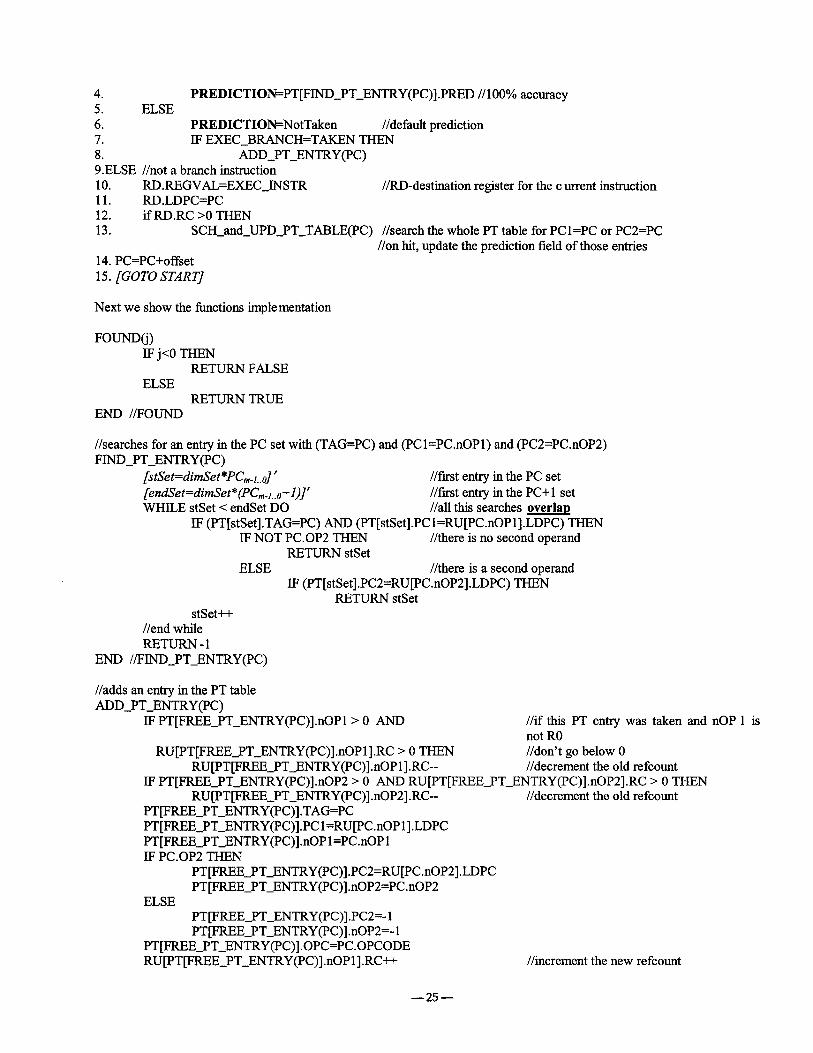
4. PREDICTION=PT[FIND PT ENTRY(PC)].PRED//100% accuracy 5. ELSE 6. PREDICTION=NotTaken //default prediction 7. IF EXEC BRANCH=TAKEN THEN 8. ADD PT ENTRY(PC) 9.ELSE //not a branch instruction 10. RD.REGVAL=EXEC_INSTR //RD-destination register for the current instruction 11. RD.LDPC=PC 12. ifRD.RC >0 THEN 13. SCH_and_UPD PT TABLE(PC) //search the whole PT table for PC i=PC or PC2=PC

//on hit, update the prediction field of those entries 14. PC=PC+offset 15. [GOTO START]

Next we show the functions implementation

FOUND(j) IF j<O THEN

RETURN FALSE ELSE

RETURN TRUE END //FOUND

//searches for an entry in the PC set with (TAG=PC) and (PCI=PC.nOP1) and (PC2=PC.nOP2) FIND PT ENTRY(PC)

[stSet=dimSet*PCm.L.d" //first entry in the PC set [endSet=dimSet*(PCm.L.o+l)] ' //first entry in the PC+I set WHILE stSet < endSet DO //all this searches overlap

IF (PT[stSet].TAG=PC) AND (PT[stSet].PCI=RU[PC.nOP1].LDPC) THEN IF NOT PC.OP2 THEN //there is no second operand

RETURN stSet ELSE //there is a second operand

IF (PT[stSet].PC2=RU[PC.nOP2].LDPC) THEN RETURN stSet

stSet++ //end while RETURN - 1

END //FIND PT ENTRY(PC)

//adds an entry in the PT table ADD PT ENTRY(PC)

IF PT[FREE PT ENTRY(PC)].nOP1 > 0 AND

RU[PT[FREE PT ENTRY(PC)].nOP1].RC > 0 THEN RU[PT[FREE PT ENTRY(PC)].nOP1].RC--

//if this PT entry was taken and nOP 1 is not R0 //don't go below 0 //decrement the old refcount

IF PT[FREE PT ENTRY(PC)].nOP2 > 0 AND RU[PT[FREE PT ENTRY(PC)].nOP2].RC > 0 THEN RU[PT[FREE_PT_ENTRY(PC)].nOP2].RC- //decrement the old refcount

PT[FREE PT ENTRY(PC)].TAG=PC PT[FREE_PT_ENTRY(PC)].PC 1 =RU[PC .nOP 1 ].LDPC PT[FREE PT ENTRY(PC)].nOPI=PC.nOP1 IF PC.OP2 THEN

PT [FREE_PT_ENTRY(PC)] .PC2=RU[PC.nOP2] .LDPC PT[FREE PT ENTRY(PC)].nOP2=PC.nOP2

ELSE PT[FREE PT ENTRY(PC)].PC2=-I PT[FREE PT ENTRY(PC)].nOP2=-I

PT[FREE PT ENTRY(PC)] .OPC=PC.OPCODE RU[PT[FREE PT ENTRY(PC)].nOP1].RC++ //increment the new refcount

25

IF PC.OP2 THEN RU[PT[FREE PT ENTRY(PC)].nOP2].RC++

END //ADD PT ENTRY //increment the new refcount

//full PT table search for PC in PC 1 or PC2 fields SCH and UPD PT TABLE(PC)

9=0] //this long time searches may overlap with EXEC_INSTR or data reuse process WHILE j<dimPT DO

IF (PT[j].PC I=PC) OR (PT[j].PC2=PC) THEN PT[j].PRED=EXEC(PT[j].OPC, RU[PTD].nOP 1 ].REGVAL,

RU[PTD ].nOP2].REGVAL) j++

END //SCH andI.JPD PT TABLE

References

[1] The SimpleScalar Tool Set. Technical Report CS-TR- 96-1308, University of Wisconsin-Madison, July, 1996 (www.cs.wisc.edu/,~rnscalar/simplescalar.html)

[2] Vintan L. - Towards a High Performance Neural Branch Predictor, Proceedings of The International Joint Conference on Neural Networks - IJCNN '99 (CD-ROM, ISBN 0-7803-5532-6), Washington DC, USA, 10-16 July, 1999

[3] B. Calder, D. Grunwald, D. Lindsay - Corpus-Based Static Branch Prediction, ACM Sigplan Notices, vol. 30, No. 6, pages 79-91, June, 1995, ISBN 0-89791-697-2

[4] L. Vintan - Instruction Level Parallel Processors, Romanian Academy Publishing House, Bucharest, 2000 (264 pp., in Romanian), ISBN 973 -27-0734-8

[5] G. Steven, C. Egan, L. Vintan - Dynamic Branch Prediction using Neural Networks, Proceedings of International Eurornicro Conference DSD '2001,Warsaw, Poland, September, 2001

[6] G. Steven, C. Egan, W. Shim, L. Vintan - Applying Caching to Two-Level Adaptive Branch Prediction, Proceedings of International Euromicro Conference DSD '2001, Warsaw, Poland, September, 2001

[7] C. Egan, G. Steven, L. Vintan - Quantgfying the Benefits of Multiple Prediction Stages in Cached Two Level Adaptive Branch Predictors, Proceedings of International Conference SBAC-PAD, Brasil, Braslia, September, 2001

[8] S. Sechrest, C. Lee, Mudge T. - The Role of Adaptivity in Two-level Adaptive Branch Prediction, 28 th ACM / IEEE International Symposium on Microarchitecture, November 1995.

[9] T. Yeh, Y.N. Part - Two-Level Adaptive Branch Prediction, 24 t~ ACM / IEEE International Symposium on Microarchitecture, November 1991.

[10] T. Yeh, Y.N. Part - Alternative Implementation of Two-Level Adaptive Branch Prediction, 19 th Annual International Symposium on Computer Science, May 1995.

[11] G. Steven et al. - A Superscalar Architecture to Exploit Instruction Level Parallelism, Microprocessors and Microsystems, No 7, 1997.

[12] SPEC The SPEC benchmark programs (www.spec.orN

[13] W.F. Wong - Source Level Static Branch Prediction, The Computer Journal, vol. 42, No.2, 1999

[14] J. Stark, M. Evers, Y. Patt - Variable Length Path Branch Prediction, ASPLOS VIII 10/98, CA, USA, 1998

[15] M. Evers, S. Patel, R. Chappell, Y. Patt - A n Analysis of Correlation and Predictability: What Makes Two Level Branch Prediction Work, ISCA, Barcelona, June 1998

[16] L. Vintan, C. Egan - Extending Correlation in Branch Prediction Schemes, Proceedings of 25 th Euromicro International Conference, Milano, Italy, 8 -10 September, IEEE Computer Society Press, ISBN 0-7695- 0321-7, 1999

[17] L. Vintan - Towards a Powerful Dynamic Branch Predictor, Romanian Journal of Information Science and Technology (ROMJIST), vol.3, nr.3, pg.287-301, ISSN: 1453-8245, Romanian Academy, Bucharest, 2000

[18] Collins R. -Exploiting Parallelism in a Superscalar Architecture, PhD Thesis, University of Hertfordshire, U.K., 1996

26

[19] Steven G., Egan C., Anguera R., Vintan L. - Dynamic Branch Prediction using Neural Networks, Proceedings of International Eurornicro Conference DSD

'2001, ISBN 0-7695-1239-9, Warsaw, September, 2001 (pg. 178-185)

Poland,

Table 1. Benchmark

Benchmarks App1u Apsi Ccl Compress95

SPEC '95 benchmarks Input Inst. Count executed

applu.in 500000000 apsi.in 500000000 lstmt.i 500000000 bigtest.in 500000000

Fpppp Hydro Ijpeg Li M~rid Perl Su2cor Swim

natoms.in 500000000 hydro2d.in 500000000

500000000 vigo.ppm *Asp m d.in scrabbl.pl su2cor.in swim.in

500000000 500000000 500000000 500000000 500000000

Tomcatv tomcatv.in 500000000 Turb3d

Wave5

turb3d.in 500000000

wave5.in 500000000

'ograms and inputs Stanford lISA benehmarks

Benchmarks Inst. Count executed fbubble

Ir~ut Null 875174

fmatrix Null 824443 fperm Null 581099 fpuzzle Null 25271829 fqueens Null 365205 Fsort Null 198305 Ftower Null 459788 Ftree Null 267642

:PC il

:B:

PC:(

Figure I. The new proposed prediction scheme. A) when a non-branch instruction is encountered," B) when a branch instruction is encountered

27

A:. . . . '~aiue;. ~ : u ~ c:..

:i:p! i:9~ ::r~:!r2:i ~ I' :J ":: : ;: . , 0

: :1 • * : : d o n ~ h i n g ::.

B i! :0:' :o . ~15 0

:::el :,.a.~tl :::r3:.f3frT:..:~ ~e~. ]

do nothtng

Figure 2. Example o f the first instance of a particular branch; .4), B) actions took when issuing non-branch instructions; C) actions took before b l branch execution

:::ip:~:::r~i ~, :mi;2;~::,

a :!b:Zan:d : r 3 i i g ; t T : ~

,yo o .i

!",0: i , i 1

:vaitie :i::~DI~C i:RC,! ,,TAGPC1PC2DPCnQPInO~2PREDLRIJ:. R 0 ~0 ,: 0 I t

J e 1

:;i~2i~:::i~ne ,:~3~

Figure 3. Example o f the second instance of a particular branch; A), B) actions took when issuing non-branch instructions; C) actions took before b2 branch execution

m 2 8 m

1

0,98

0,96

0,94

0,92

64 128 256 512 1024 2048

¢ PCBANT=0]

-.D.-- PCB ANT=I I

Figure 4. PCB' s average "prediction" accuracy obtained on Stanford benchmarks

1

0,93

0,~

0,83

0,It

0,73

0,7

IO PCB ANT=0 I El PCB ANT=I I

I

32x4 64x4 128x4 256x4 512x4

Figure 5. PCB' s average 'prediction" accuracy obtained on SPEC "95 benchmarks

1

0,95,

0,9,

0,85,

0,8,

0,75

0,7,

I I I CB ANT=0 O BTB set-assoc Q BTB full-assoc

32x4 64x4 128x4 256x4 512x4

Figure 6. Average "prediction" accuracies obtained on SPEC '95 benchmarks

29