
An alternative method for inducing a membership function of a category
28
An Alternative Method for Inducing a Membership Function of a Category Hiroshi Narazaki Electronics Research Laboratory Kobe Steel, Ltd., Kobe, Japan Anca L. Ralescu Laboratory for International Fuzzy Engineering Research, Naka-ku, Yokohama, Japan ABSTRACT We propose an alternative learning method for category classification knowledge. Our method induces a membership function for a category from positive and negative examples. It can learn "topological knowledge" such as typicality of an example. Our method consists of two stages: example space configuration of a coordinate system in the first stage, induction of membership function that induces a membership function based on the distance in the newly configured example space in the second. Further, we investigate search strategiessuitable for deriving the symbolic expression of a category by geometric analysis of the example space. KEYWORDS: Concept learning, machine learning, induction, classification knowledge, membership function, knowledge acquisition I. INTRODUCTION An important body of work exists now on the problem of concept learning where the purpose is the acquisition of classification knowledge. Address correspondence to Anca L. Ralescu, Laboratoryfor International Fuzzy Engineering Research, SibarHegnerBldg. 3F, 89-1, Yamashita-cho,Naka-ku, 231, Japan. Received March 1, 1992; accepted June 1, 1993. This work was done when H. Narazaki was a research associate at LIFE chair of Fuzzy Theory, Department of Systems Science, Tokyo Institute of Technology, Japan. A. L. Ralescu is on leave from Computer Science Department, University of Cincinnati, OH. Research partially supported by NSF Grant INT91-08632. International Journal of Approximate Reasoning 1994; 11:1-27 © 1994 Elsevier Science Inc. 655 Avenue of the Americas, New York, NY 10010 0888-613X/94/$7.00 1
Transcript of An alternative method for inducing a membership function of a category
An Alternative Method for Inducing a Membership Function of a Category
Hiroshi Narazaki Electronics Research Laboratory
Kobe Steel, Ltd., Kobe, Japan
Anca L. Ralescu Laboratory for International Fuzzy Engineering Research,
Naka-ku, Yokohama, Japan
A B S T R A C T
We propose an alternative learning method for category classification knowledge. Our method induces a membership function for a category from positive and negative examples. It can learn "topological knowledge" such as typicality of an example. Our method consists of two stages: example space configuration of a coordinate system in the first stage, induction of membership function that induces a membership function based on the distance in the newly configured example space in the second. Further, we investigate search strategies suitable for deriving the symbolic expression of a category by geometric analysis of the example space.
K E Y W O R D S : Concept learning, machine learning, induction, classification knowledge, membership function, knowledge acquisition
I. INTRODUCTION
A n i m p o r t a n t body of work exists now on the p rob lem of concept
learning where the purpose is the acquisi t ion o f classification knowledge.
Address correspondence to Anca L. Ralescu, Laboratory for International Fuzzy Engineering Research, Sibar Hegner Bldg. 3F, 89-1, Yamashita-cho, Naka-ku, 231, Japan.
Received March 1, 1992; accepted June 1, 1993. This work was done when H. Narazaki was a research associate at LIFE chair of Fuzzy
Theory, Department of Systems Science, Tokyo Institute of Technology, Japan. A. L. Ralescu is on leave from Computer Science Department, University of Cincinnati, OH. Research partially supported by NSF Grant INT91-08632.
International Journal of Approximate Reasoning 1994; 11:1-27 © 1994 Elsevier Science Inc. 655 Avenue of the Americas, New York, NY 10010 0888-613X/94/$7.00 1
2 Hiroshi Narazaki and Anca L. Ralescu
One of the most successful methods is the ID3 family, originating from Quinlan [1-3]. Based on an information theoretical approach, these meth- ods generate a decision tree to classify an example to a category. Among other works are Michalski's inductive logic [4] and Mitchel's version space method [5], to name only a few.
The primary concern for the above methods is to generate a "readable" symbolic expression for a category that can also be used as a classification rule. The efforts are focused on a search for the simplest logical expression consistent with the observed examples. In general, the quality and effi- ciency of the learning mechanism are constrained by the form of knowl- edge representation, the vocabulary available for category description, and by the search strategy. These are assumed to be given prior to the learning task. Such background knowledge is generally called the "bias" of the learning mechanism [6].
Another approach is a quantitative approach that is based on techniques such as discriminant functions, statistical analysis, and neural networks [7-13]. The classification knowledge is represented by a discriminant function, and the learning is a problem to estimate the optimum parame- ter values of a given mathematical formula for a discriminant function. The advantage of this approach is that it can effectively cope with issues concerning topological aspects of the category based on geometric notions. In other words, we can answer questions such as "How sure is the classification?", "What is the most typical example?" and "Is a misclassi- fled example exceptional or on the fuzzy zone of the category?". The bias in this approach is represented by a mathematical formula chosen for a discriminant function and optimization strategies.
Comparing the two approaches, it seems reasonable to adopt a way that combines them. The topological aspect is not only practically useful but also necessary when considering the vagueness of the category definition. As originally claimed by Wittgenstein, the concept can only be formed as a "family of resemblances" and the "ideal language" for its sufficient and necessary definition is not likely to exist [14]. Thus similarity, typicality, or conceptual distance between categories becomes necessary to deal with the inexact or partial match of an example to a category. However, we still definitely need a symbolic interface because the learning process is in- evitably interactive and we need some explanatory mechanism based on symbols or language.
Along this line, efforts for integrating the two approaches have been made. In [15], a method to incorporate the frequency-based typicality measure into the symbolic representation based on Sowa's conceptual graphs was proposed.
In this study we put forward an alternative method for the same type of problem. First we show the outline of our problem and method by using a simple example extracted from [3] and discuss the features of our method.
Alternative Method for Inducing a Membership Function 3
As usual, an example is given as a set of attribute-value pairs like
e = {(Ai, aiy);i = 1,2 . . . . , n , j = 1,2 . . . . ,li}
where A i is an attribute and aij is one of its possible values. We suppose that we have a finite number of n attributes and l i values for each attribute A i. Further we assume that we are given enough attributes to distinguish among categories.
Our method consists of two stages: example space configuration and induction of membership function as explained in the following paragraphs.
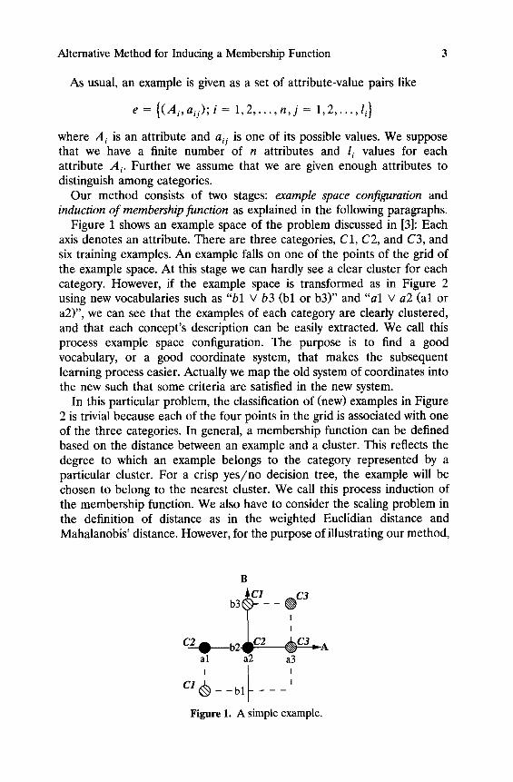
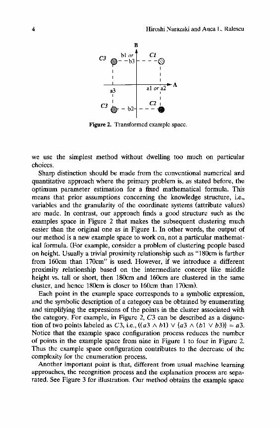
Figure 1 shows an example space of the problem discussed in [3]: Each axis denotes an attribute. There are three categories, C1, C2, and C3, and six training examples. An example falls on one of the points of the grid of the example space. At this stage we can hardly see a clear cluster for each category. However, if the example space is transformed as in Figure 2 using new vocabularies such as "bl v b3 (bl or b3)" and "a l v a2 (al or a2)", we can see that the examples of each category are clearly clustered, and that each concept's description can be easily extracted. We call this process example space configuration. The purpose is to find a good vocabulary, or a good coordinate system, that makes the subsequent learning process easier. Actually we map the old system of coordinates into the new such that some criteria are satisfied in the new system.
In this particular problem, the classification of (new) examples in Figure 2 is trivial because each of the four points in the grid is associated with one of the three categories. In general, a membership function can be defined based on the distance between an example and a cluster. This reflects the degree to which an example belongs to the category represented by a particular cluster. For a crisp yes /no decision tree, the example will be chosen to belong to the nearest cluster. We call this process induction of the membership function. We also have to consider the scaling problem in the definition of distance as in the weighted Euclidian distance and Mahalanobis' distance. However, for the purpose of illustrating our method,
B
b3 'C cq -b2 c3_ - A
a l a2 a3
C1 - - b l _ _ _ I
F i g u r e 1. A s i m p l e e x a m p l e .
4 Hiroshi Narazaki and Anca L. Ralescu
bl o r C3 ~ _ -b3
I I
I
a3 I
I
C3 ~ _ _ b2-
C1
I
I
I - "A al or a2
I
I C2
Figure 2. Transformed example space.
we use the simplest method without dwelling too much on particular choices.
Sharp distinction should be made from the conventional numerical and quantitative approach where the primary problem is, as stated before, the optimum parameter estimation for a fixed mathematical formula. This means that prior assumptions concerning the knowledge structure, i.e., variables and the granularity of the coordinate systems (attribute values) are made. In contrast, our approach finds a good structure such as the examples space in Figure 2 that makes the subsequent clustering much easier than the original one as in Figure 1. In other words, the output of our method is a new example space to work on, not a particular mathemat- ical formula. (For example, consider a problem of clustering people based on height. Usually a trivial proximity relationship such as "180cm is farther from 160cm than 170cm" is used. However, if we introduce a different proximity relationship based on the intermediate concept like middle height vs. tall or short, then 180cm and 160cm are clustered in the same cluster, and hence 180cm is closer to 160cm than 170cm).
Each point in the example space corresponds to a symbolic expression, and the symbolic description of a category can be obtained by enumerating and simplifying the expressions of the points in the cluster associated with the category. For example, in Figure 2, C3 can be described as a disjunc- tion of two points labeled as C3, i.e., ((a3 /~ bl) v {a3 /x (bl v b3)} = a3. Notice that the example space configuration process reduces the number of points in the example space from nine in Figure 1 to four in Figure 2. Thus the example space configuration contributes to the decrease of the complexity for the enumeration process.
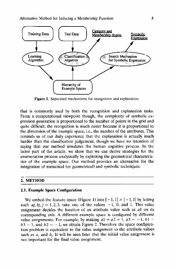
Another important point is that, different from usual machine learning approaches, the recognition process and the explanation process are sepa- rated. See Figure 3 for illustration. Our method obtains the example space
Alternative Method for Inducing a Membership Function 5
Q Training Data 1
(
Test Data 1
Hierarchy of Example Spaces
Membershin dem, ee Symbolic Exmession
)
y Figure 3. Separated mechanisms for recognition and explanation.
that is commonly used by both the recognition and explanation tasks. From a computational viewpoint though, the complexity of symbolic ex- pression generation is proportional to the number of points in the grid and quite difficult; the recognition is much easier because it is proportional to the dimension of the example space, i.e., the number of the attributes. This reminds us of our daily experience that the explanation is actually much harder than the classification judgement, though we have no intention of saying that our method simulates the human cognitive process. In the latter part of the article, we show that we can derive strategies for the enumeration process analytically by exploiting the geometrical characteris- tics of the example space. Our method provides an alternative for the integration of numerical (or geometrical) and symbolic techniques.
2. METHOD
2.1. Example Space Configuration
We embed the feature space (Figure 1) into [ - 1, 1] × [ - 1, 1] by letting each aj, bj, j = 1, 2, 3, take one of the values -1 , 0, and 1. This value assignment decides the location of an attribute value such as al on its corresponding axis. A different example space is configured by different value assignments. For example, by making al = a2 = 1, a3 = -1 , bl = b3 = 1, and b2 = -1 , we obtain Figure 2. Therefore the space configura- tion problem is equivalent to the value assignment to the attribute values such as aj and bj. It will be seen later that the initial value assignment is not important for the final value assignment.
6 Hiroshi Narazaki and Anca L. Ralescu
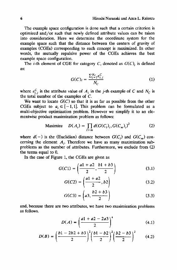
The example space configuration is done such that a certain criterion is optimized and/or such that newly defined attribute values can be taken into consideration. Here we determine the coordinate system for the example space such that the distance between the centers of gravity of examples (CGEs) corresponding to each concept is maximized. In other words, the mutually repulsive power of the CGEs achieves the best example space configuration.
The i-th element of CGE for category C, denoted as G(C) i is defined a s ;
vi-, N c _C G(C)i "~= lei' j (1)
Nc
where e c. is the attribute value of A i in the j-th example of C and N c is t,J the total number of the examples of C.
We want to locate G(C) so that it is as far as possible from the other CGEs subject to a i ~ [ -1 ,1] . This problem can be formulated as a multi-objective optimization problem. However we simplify it to an ele- mentwise product maximization problem as follows:
Maximize O ( A i ) = 1-I d(G(Ct)~, a ( C m ) i )2 (2) l>m
where d ( - ) is the (Euclidian) distance between G(C I) and G(C m) con- cerning the element Ai. Therefore we have as many maximization sub- problems as the number of attributes. Furthermore, we exclude from (2) the terms equal to 0.
In the case of Figure 1, the CGEs are given as
(al +a2 bl +b3) G(C1) = 2 ' 2 (3.1)
( a l + a 2 ) O(C2) = 2 , b2 (3.2)
( b 2 + b 3 ) G(C3) = a3, ~ (3.3)
and, because there are two attributes, we have two maximization problems as follows.
( aa + a2 - 2a3 ) 4 D(A) = 2 (4.1)
Alternative Method for Inducing a Membership Function 7
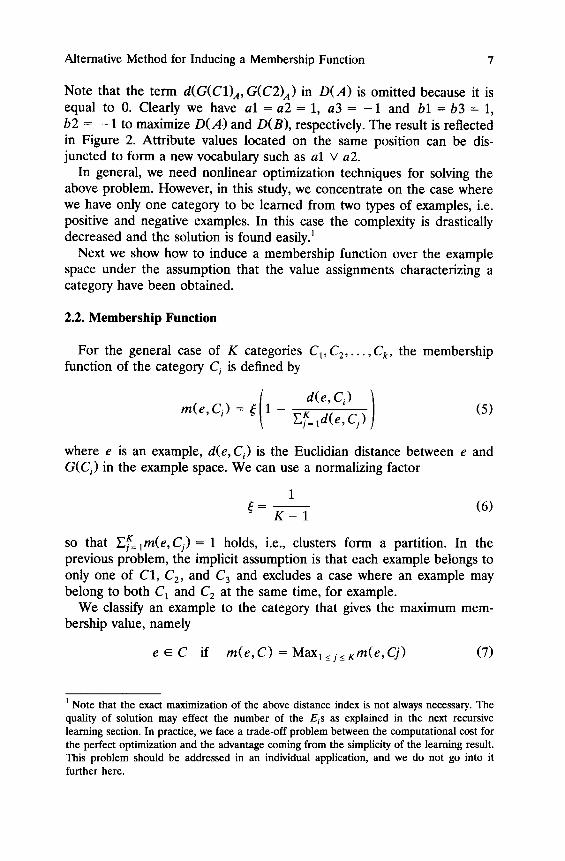
Note that the term d(G(C1)A, G(C2) A) in D(A) is omitted because it is equal to 0. Clearly we have a l = a2 = 1, a3 = - 1 and bl = b3 = 1, b2 = - 1 to maximize D(A) and D(B), respectively. The result is reflected in Figure 2. Attribute values located on the same position can be dis- juncted to form a new vocabulary such as a l v a2.
In general, we need nonlinear optimization techniques for solving the above problem. However, in this study, we concentrate on the case where we have only one category to be learned from two types of examples, i.e. positive and negative examples. In this case the complexity is drastically decreased and the solution is found easily)
Next we show how to induce a membership function over the example space under the assumption that the value assignments characterizing a category have been obtained.
2.2. Membership Function
For the general case of K categories C1, C 2 . . . . . C k, the membership function of the category C i is defined by
m(e,Ci) = so(1 d(e, Ci) )
E~= td(e, Cj) (5)
where e is an example, d(e, Ci) is the Euclidian distance between e and G(C i) in the example space. We can use a normalizing factor
= - - (6) K - 1
so that E~=xm(e,C)= 1 holds, i.e., clusters form a partition. In the previous problem, the implicit assumption is that each example belongs to only one of C1, C2, and C 3 and excludes a case where an example may belong to both C 1 and C 2 at the same time, for example.
We classify an example to the category that gives the maximum mem- bership value, namely
e ~ C if m(e,C) =MaxlzjzKm(e,C j) (7)
1 Note that the exact maximization of the above distance index is not always necessary. The quality of solution may effect the number of the Eis as explained in the next recursive learning section. In practice, we face a trade-off problem between the computational cost for the perfect optimization and the advantage coming from the simplicity of the learning result. This problem should be addressed in an individual application, and we do not go into it further here.
8 Hiroshi Narazaki and Anca L. Ralescu
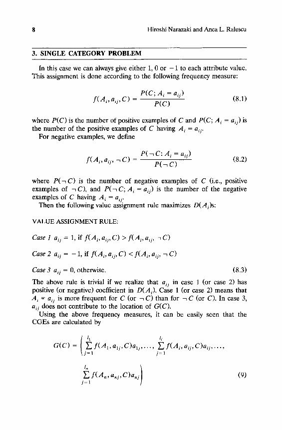
3. SINGLE CATEGORY PROBLEM
In this case we can always give either 1, 0 or - 1 to each attribute value. This assignment is done according to the following frequency measure:
P ( C ; A i = air) (8.1) f ( h i, aij, C) = P ( C )
where P ( C ) is the number of positive examples of C and P(C; A i the number of the positive examples of C having A i = air.
For negative examples, we define
= air) is
P(--nC: A i = aij) f ( A i , a i j , -~C) = P ( ~ C ) (8.2)
where P ( ~ C) is the number of negative examples of C (i.e., positive examples of --1C), and P(-~ C; A i = aij) is the number of the negative examples of C having A i = air.
Then the following value assignment rule maximizes D(Ai)s:
VALUE ASSIGNMENT RULE:
Case 1 air = 1, if f ( A i , aij , C) > f ( A i, air, --7 C)
Case 2 air = - 1, if f ( A i, aij , C) < f ( A i , air, --1 C)
Case 3 air = 0, otherwise. (8.3)
The above rule is trivial if we realize that air in case 1 (or case 2) has positive (or negative) coefficient in D(Ai ) . Case 1 (or case 2) means that A i = aij is more frequent for C (or -1 C) than for -1 C (or C). In case 3, air does not contribute to the location of G(C).
Using the above frequency measures, it can be easily seen that the CGEs are calculated by
1~=1 li G ( C ) = f ( A l , a l j , C ) a l j . . . . , E f (A i ,a i j ,C)a i j . . . . .
j= j = l
,n ) ~_, f ( A n , anj, C)anj
j = l (9)
Alternative Method for Inducing a Membership Function 9
where aij ~ { - 1, 0, 1} as determined by the above value assignment rule. The membership function is also simplified because we have only {C i} = {C, ~ C} and ~ becomes 1.
We demonstrate the above method using an example from [1].
3.1. "Saturday Morning" Category
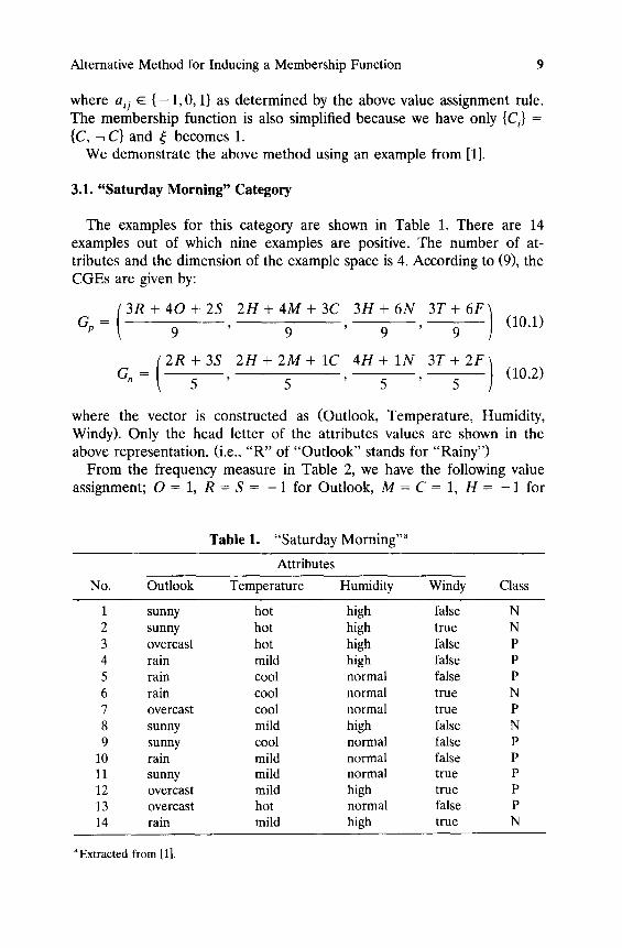
The examples for this category are shown in Table 1. There are 14 examples out of which nine examples are positive. The number of at- tributes and the dimension of the example space is 4. According to (9), the CGEs are given by:
3 R + 4 0 + 2 S 2 H + 4 M + 3 C 3 H + 6 N 3 T + 6 F Gp = 9 ' 9 ' 9 ' 9 ) (10.1)
2 R + 3 S 2 H + 2 M + 1C 4 H + 1N 3 T + 2 F G. = 5 ' 5 ' 5 ' 5 ) (10.2)
where the vector is constructed as (Outlook, Temperature , Humidity, Windy). Only the head letter of the attributes values are shown in the above representation. (i.e., " R " of "Out look" stands for "Rainy")
From the frequency measure in Table 2, we have the following value assignment; O = 1, R = S = - 1 for Outlook, M = C = 1, H = - 1 for
Table 1. "Saturday Morning ''a
Attributes
No. Outlook Temperature Humidity Windy Class
1 sunny hot high false N 2 sunny hot high true N 3 overcast hot high false P 4 rain mild high false P 5 rain cool normal false P 6 rain cool normal true N 7 overcast cool normal true P 8 sunny mild high false N 9 sunny cool normal false P
10 rain mild normal false P 11 sunny mild normal true P 12 overcast mild high true P 13 overcast hot normal false P 14 rain mild high true N
aExtracted from [1].
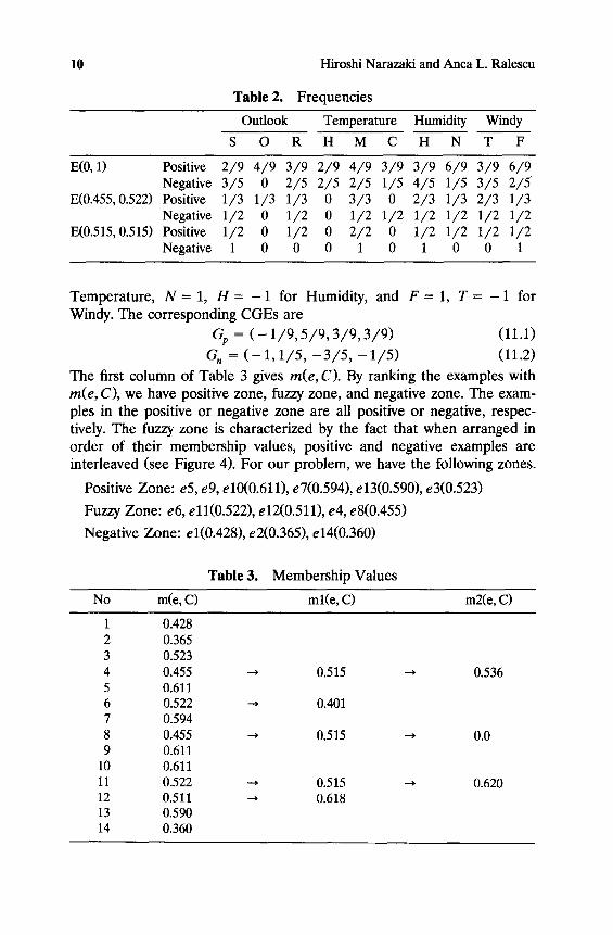
10 Hiroshi Narazaki and Anca L. Ralescu
Table 2. Frequencies
Outlook Temperature Humidity Windy
S O R H M C H N T F
E(0,1) Positive 2/9 4/9 3/9 2/9 4/9 3/9 3/9 6/9 3/9 6/9 Negative 3/5 0 2/5 2/5 2/5 1/5 4/5 1/5 3/5 2/5
E(0.455,0.522) Positive 1/3 1/3 1/3 0 3/3 0 2/3 1/3 2/3 1/3 Negative 1/2 0 1/2 0 1/2 1/2 1/2 1/2 1/2 1/2
E(0.515,0.515) Positive 1/2 0 1/2 0 2/2 0 1/2 1/2 1/2 1/2 Negative 1 0 0 0 1 0 1 0 0 1
Temperature, N = 1, H = - 1 for Humidity, and F = 1, T = - 1 for Windy. The corresponding CGEs are
Gp = ( - 1/9, 5 /9 , 3/9, 3 /9) (11.1)
G, = ( - 1, 1/5, - 3 / 5 , - 1/5) (11.2)
The first column of Table 3 gives re(e, C). By ranking the examples with m(e, C), we have positive zone, fuzzy zone, and negative zone. The exam- ples in the positive or negative zone are all positive or negative, respec- tively. The fuzzy zone is characterized by the fact that when arranged in order of their membership values, positive and negative examples are interleaved (see Figure 4). For our problem, we have the following zones.
Positive Zone: e5, e9, el0(0.611), e7(0.594), e13(0.590), e3(0.523)
Fuzzy Zone: e6, e11(0.522), e12(0.511), e4, e8(0.455)
Negative Zone: e1(0.428), e2(0.365), e14(0.360)
Table 3. Membership Values
No m(e, C) ml(e, C) m2(e, C)
1 0.428 2 0.365 3 0.523 4 0.455 5 0.611 6 0.522 7 0.594 8 0.455 9 0.611
10 0.611 11 0.522 12 0.511 13 0.590 14 0.360
0.515
--* 0.401
0.515 ---,
0.515 0.618
0.536
0.0
0.620
Alternative Method for Inducing a Membership Function 11
C a s e I
Negative Examples
0
Negative Zone
I I
I ~ I
I Fuzzy i Z o n e I
PoMaveZone
Membership Degree
Positive Examples
Case 2
o I
I V a c u u m Negative II~ I Examples Negative Zone Zone
Membership ~t+ 1 Degree
I Positive I Positive Zone Examples I
(Nofuzzy zone)
Case 3
Membership 0 ~'~ ~ 1 Degree
I I ~ Positive Zone I Positive
I Examples Negative I -.- Examples I Negative Zone v I
I (Exceptional Examples)
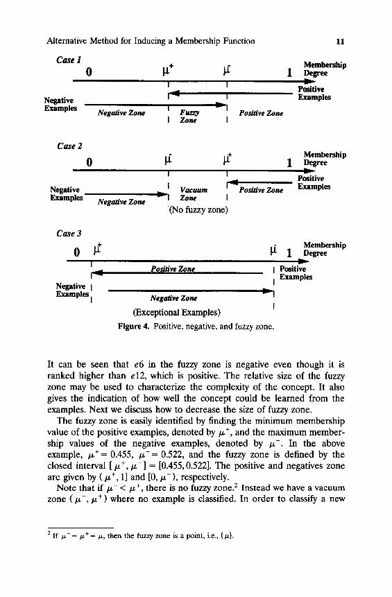
Figure 4. Positive, negative, and fuzzy zone.
It can be seen that e6 in the fuzzy zone is negative even though it is ranked higher than el2, which is positive. The relative size of the fuzzy zone may be used to characterize the complexity of the concept. It also gives the indication of how well the concept could be learned from the examples. Next we discuss how to decrease the size of fuzzy zone.
The fuzzy zone is easily identified by finding the minimum membership value of the positive examples, denoted by/z +, and the maximum member- ship values of the negative examples, denoted by p~-. In the above example, /~+= 0.455, /x-= 0.522, and the fuzzy zone is defined by the closed interval [/z +, /z-] = [0.455, 0.522]. The positive and negatives zone are given by (/z +, 1] and [0, ~ - ) , respectively.
Note that i f / z - < /z +, there is no fuzzy zone. 2 Instead we have a vacuum zone ( /~- , /z +) where no example is classified. In order to classify a new
2 If IX- = Ix+ = Ix, then the fuzzy zone is a point, i.e., {Ix}.
12 Hiroshi Narazaki and Anca L. Ralescu
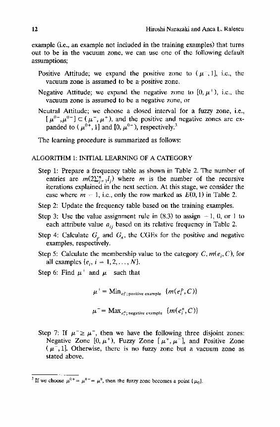
example (i.e., an example not included in the training examples) that turns out to be in the vacuum zone, we can use one of the following default assumptions;
Positive Attitude; we expand the positive zone to ( /z- , 1], i.e., the vacuum zone is assumed to be a positive zone.
Negative Attitude; we expand the negative zone to [0,/z+), i.e., the vacuum zone is assumed to be a negative zone, or
Neutral Attitude; we choose a closed interval for a fuzzy zone, i.e., [ /x°- ,~ °+] c (/z-,/~+), and the positive and negative zones are ex- panded to (/z °+, 1] and [0,/x °- ), respectively. 3
The learning procedure is summarized as follows:
ALGORITHM 1: INITIAL LEARNING OF A CATEGORY
Step 1: Prepare a frequency table as shown in Table 2. The number of entries are m(2]ET=l/j) where m is the number of the recursive iterations explained in the next section. At this stage, we consider the case where m = 1, i.e., only the row marked as E(0, 1) in Table 2.
Step 2: Update the frequency table based on the training examples.
Step 3: Use the value assignment rule in (8.3) to assign - 1 , 0, or 1 to each attribute value aij based on its relative frequency in Table 2.
Step 4: Calculate Gp and Gn, the CGEs for the positive and negative examples, respectively.
Step 5: Calculate the membership value to the category C, m(e i, C), for all examples {e i, i = 1, 2 . . . . . N}.
Step 6: Find /z + and /~ such that
I.L += {m( eiP, C)} Min ef; positive example
/z- = Maxe,; negative example { m(en, C)}
Step 7: If /z > / x +, then we have the following three disjoint zones: Negative Zone [0,/~+), Fuzzy Zone [/z +,/z-], and Positive Zone ( /z- , 1]. Otherwise, there is no fuzzy zone but a vacuum zone as stated above.
3 If we choose /x °+= /z °-= /z °, then the fuzzy zone becomes a point {/-to}.
Alternative Method for Inducing a Membership Function 13
REMARK: Algorithm 1 does not include any heuristic search in looking for the CGEs. The computational complexity is proportional to the num- ber of examples, i.e., O(N) where N is the number of training data.
For classification of a new example e, if m(e, C) is in the positive (or negative) zone, it is recognized as Positive (or Negative). If it is in the fuzzy zone, we cannot determine its category. To reduce this fuzziness, we apply the recursive learning procedure explained below.
4. IMPROVEMENT OF PRECISION
4.1. Recursive Learning and Classification
We denote the set of examples in the fuzzy zone as
E(tz+,tz ) = {e;tz+ <_ rn(e,C) </z-} (12)
We iterate the learning process by narrowing down the training examples to those in the fuzzy zone until the fuzzy zone becomes a null set. We call this procedure recursive learning. The recursive learning gives the follow- ing collections of training examples:
E(0, 1) ___ E(/z? , /z~ ) _~ ... _ E(/z~ + , / ~ ) 2 "'" (13)
where E(0, 1) contains all examples and E(/z~-, ~{ ) is a set of fuzzy zone examples in E(0, 1). We abbreviate E(/z 7,/z 7) as E i and we denote E(0, 1) as E 0. Each E i is associated with its own coordinate system, CGEs and the membership function mi(e, C). By ranking the examples according mi(e~C), we can find the fuzzy zone, El+l, of E i.
Our concern is whether the above recursive procedure terminates. For this discussion, we introduce the notion of exceptional examples.
Let's define e/L and e/U of E i such that
mi(e L, C) = Mint, E E, mi(ej, C)
mi(eU, C) = Max~E E, mi(ej ,C)
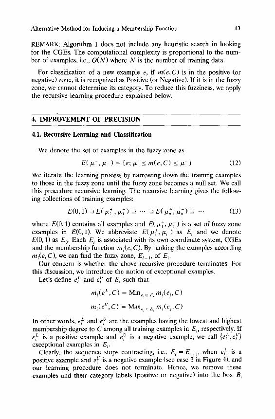
In other words, e~ and e~ are the examples having the lowest and highest membership degree to C among all training examples in E,, respectively. If ep is a positive example and e~ is a negative example, we call {e~, e~} exceptional examples in E~.
Clearly, the sequence stops contracting, i.e., E, = E~÷ 1, when e~ is a positive example and e~ is a negative example (see case 3 in Figure 4), and our learning procedure does not terminate. Hence, we remove these examples and their category labels (positive or negative) into the box B~
14 Hiroshi Narazaki and Anca L. Ralescu
for exceptional examples corresponding to E i. This ensures that after a finite number of steps, K, { E i} is strongly contracted, i.e., E i ~ Ei+ 1 and EK = &4 Notice that /z- </~+ holds and a vacuum zone exists in E r.
In summary, our learning procedure is described below.
ALGORITHM 2: Recursive Learning
Initial Values: i ~ 0; ?examples ~ E 0 (i.e., All training examples) Begin
If ?examples is empty, then exit. Else Execute the following steps:
Begin 1. Fill the frequency table and assign - 1 , 0, or 1 to attribute
values. 2. Identify negative zone, fuzzy zone, and positive zone based
on the CGEs in E i. 3. Extract examples in the fuzzy zone. 4. If the fuzzy zone examples coincide with ?examples, then
remove exceptional examples into Bi with their category labels.
5. Call Learn with ?examples ~ (Fuzzy zone examples) and i ~ i + l .
End End
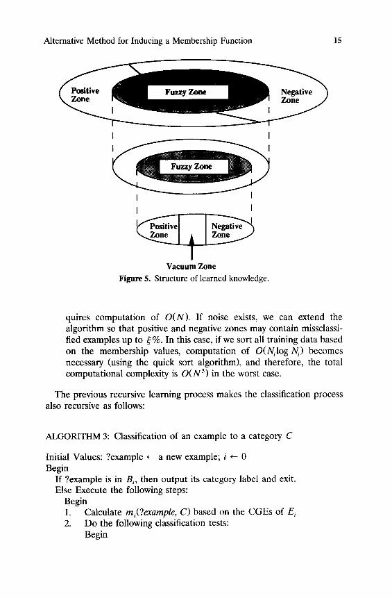
At each level E~, as illustrated in Figure 5, our learned knowledge consists of
1. CGEs for the positive and negative examples in E~, 2. /x ÷ and /z- that define the positive, negative, and fuzzy zones, and 3. exceptional examples, if any.
REMARKS:
1. Let N/, i = 1, 2 , . . . , K, be the number of training examples in Ei.(N = Y'.~:= 1N/). As stated above, the computational complexity for learn- ing E~ is O(N/). Thus, in the worst case, the total computational complexity is O(N2). (Consider the case where only exceptional examples exist. In this case K = [N + 1/2] and N,. = N - 2(i - 1)).
2. In the previous examples, we have to find minimum and maximum membership values of the positive and negative examples. This re-
4 We need not remove both eL and e/v in B i. Removing only one of them can still achieve the strong contraction of E i. Further, notice that the existence of exceptional examples means that there are no positive and negative zones, i.e., all the other examples are in the fuzzy zone.
Alternative Method for Inducing a Membership Function 15
I I
I i
I I
V a c u u m Z o n e
Figure 5. Structure of learned knowledge.
quires computation of O(N). If noise exists, we can extend the algorithm so that positive and negative zones may contain missclassi- fled examples up to ~: %. In this case, if we sort all training data based on the membership values, computation of O(Nilog N/) becomes necessary (using the quick sort algorithm), and therefore, the total computational complexity is O(N 3) in the worst case.
The previous recursive learning process makes the classification process also recursive as follows:
ALGORITHM 3: Classification of an example to a category C
Initial Values: ?example ~ a new example; i ~ 0 Begin
If ?example is in B i, then output its category label and exit. Else Execute the following steps:
Begin 1. Calculate mi(?example, C) based on the CGEs of E i 2. Do the following classification tests:
Begin
16 Hiroshi Narazaki and Anca L. Ralescu
End End
End
If ?example belongs to the positive zone, then output Positive and exit. Else If ?example belongs to the negative zone, then output Negative and exit. Else ?example belongs to the fuzzy zone, and call Classify with ?example and i ~- i + 1
First we have to look into B i to check whether the example to be classified is the same as those stored in B i. If not, the membership degree is calculated based on the CGEs of Ei. If the example is found to be in the fuzzy zone, we must move into the lower world Ei+ 1, and iterate the similar procedure. If it is in the positive or negative zone, then we can output the category label and exit.
REMARKS:
The computational complexity required for the classification is O(K) (O(N) in the worst case).
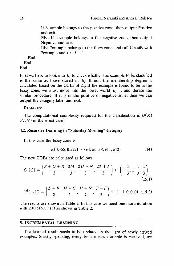
4.2. Recursive Learning in "Saturday Morning" Category
In this case the fuzzy zone is
E(0.455,0.522) = {e4, e6, e8, e l l , el2}
The new CGEs are calculated as follows.
(14)
{s+o+R 2H+N m ( 1 1 11) G I ( C ) = 3 ' 3 ' 3 ' 3 -3 ' " 3 " ' - 3
(15.1)
GI(-~C) (S+R M+C H+N T+F) . . . . . ,-- ( - 1 , 0 , 0 , 0 ) (15.2)
2 ' 2 ' 2 ' 2
The results are shown in Table 2. In this case we need one more iteration with E(0.515, 0.515) as shown in Table 2.
5. INCREMENTAL LEARNING
The learned result needs to be updated in the light of newly arrived examples. Strictly speaking, every time a new example is received, we
Alternative Method for Inducing a Membership Function 17
should update the frequency table in Table 3, and the locations of the CGEs. This also leads to the update of membership values of the examples and possibly the update of positive, negative, and fuzzy zones. In general, a relearning is necessary using the example set with the new examples added. Here we present a conservative update strategy that triggers the update only when a misclassification occurs and makes use of the fuzzy zone introduced earlier. (This can be interpreted as a case of reinforce- ment learning [16]).
A correct classification means a match of the predicted classification and the actual outcome of the new data. The new data just makes explicit the information already contained in the example space. In contrast, a misclas- sification means the mismatch and the enlargement of fuzzy zone.
Suppose that an example g is wrongly classified as negative in E i where the fuzzy zone is originally given by [ IX~+, IX7 ]. The misclassification of g means that g is in the negative zone of Ei, i.e., Ixg = mi(g, C) < IX+. After finding that g is actually positive, we should update Ix+ as Ix+= Ixg. This results in the expansion of the fuzzy zone to [ Ixg, IX-], and Ei+ i must be expanded by adding the examples in the enlarged area of the fuzzy zone, i.e., the examples in [IX g, IX+). We have to regenerate all {Ej} that are lower than Ei, i.e., {Ej; j > i + 1}. This defines a partial relearning strategy triggered by a misclassified example. The same discussions apply when g is a negative example that is wrongly classified as positive in E~.
If there is no fuzzy zone, we may be able to deal with the misclassifica- tion by changing the default assumptions for the vacuum zone, or by creating a fuzzy zone. Note that a vacuum zone exists only in E K. (Otherwise, the recursive learning continues using the examples in the fuzzy zone). In the latter case, we create EK+ 1 if mK(g,C) < IX . This defines a new fuzzy zone [mK(g, C), Ix ]. In the first case, we change the default assumption: For example, if the current default negative zone is [0, f ) (in case of a positive attitude, f = ix+), and the misclassification of g occurs such that ix < mK(g,C) < f, then we just decrease ix+ and f as ix+= mK(g, C) and f < mK(g, C), respectively.
6. CLASSIFICATION OF EXAMPLES WITH MISSING ATrRIBUTE VALUE
In practice, it often happens that some attribute values are missing either in the training or in the test examples. For the classification of an incomplete example, two approaches are usually taken: default value estimation and exhaustive check of all possible values followed by a decision making process concerning the classification. The former means a default completion of missing attribute values and it gives a point value. In
18 Hiroshi Narazaki and Anca L. Ralescu
contrast, the latter gives the interval value depending on how the comple- tion of missing attribute values are done. Notice that, in a crisp case, the interval is always vacuous, i.e., positive or negative.
If we want a thorough evaluation, the latter seems more desirable, but requires more computational cost. To avoid this, the following approxi- mate interval estimation can be used.
First we define the maximum and minimum examples: The maximum (or the minimum) example completes the missing attribute values with those corresponding 1 (or - 1 ) in E 0. For example, in case of an incomplete example "Outlook is overcast," we have two maximum examples, (O, M, N, F) and (O, C, N, F). Similarly, the minimum example is given by (O, H, H, T). The interval of the membership degree is estimated in E 0 by using these maximum and minimum examples.
We say that the estimation is correct when the maximum and minimum membership values estimated as above coincide with those obtained by exhaustively checking all possible completions. Consider the case where the maximum example is in the positive zone and the minimum example is in the negative zone of E 0. In this case, the estimation is correct. In contrast, when the minimum example is in the fuzzy zone, the estimation in E 0 may be incorrect, and we have to look into Ej, j > 0, for the thorough evaluation.
For instance, in E0, the maximum of "Outlook is overcast" is in the positive zone. However, its minimum example is in the fuzzy zone with the membership degree 0.561. The real minimum membership value is 0.506 of (O, C, H, T) in the negative zone of El. 5
7. ENUMERATING EXPRESSIONS
We consider now the task of obtaining a symbolic expression for the concept learned: The symbolic expression can be obtained by disjuncting the expressions associated with the points in the positive zone. The final example space has at most 3 n points, a decrease from the original I-IV= lli points. Here we discuss pruning strategies for a more efficient search by exploiting the geometrical characteristics of the example space.
5 This example shows that the result of our learning mechanism is different from Quinlan's result where all examples with overcast outlook are classified as positive. If we use a classification rule: "If mi(e, C) > 0.5, the e is positive," then we obtain the same result. ID3's result comes from the fact that all training examples that have overcast outlook are positive. However, in (O, C, H, T), the values for humidity and windy are more frequent in the negative examples. In other words, our method decreases the membership degree by taking into consideration the values of the other attributes.
Alternative Method for Inducing a Membership Function
x Vx gP
V G - V x
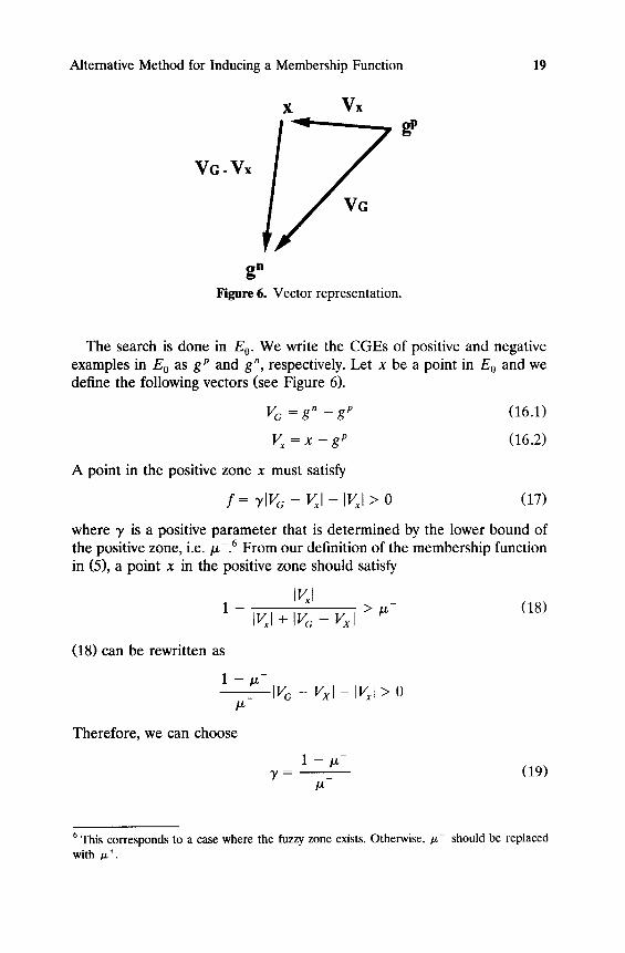
gn Figure 6. Vector representation.
19
The search is done in E 0. We write the CGEs of positive and negative examples in E 0 as gP and gn, respectively. Let x be a point in E 0 and we define the following vectors (see Figure 6).
VG = g n _ g p (16.1)
V x = x - g P (16.2)
A point in the positive zone x must satisfy
f = 3"IV c - V x [ - IV~[ > 0 (17)
where 3' is a positive parameter that is determined by the lower bound of the positive zone, i.e./z-.6 From our definition of the membership function in (5), a point x in the positive zone should satisfy
IVxl 1 - > / z - ( 1 8 )
IVxl + Iv~ - v x I
(18) can be rewritten as
1 - g -
/x-
Therefore, we can choose
- - I V G -- VxI - IVxt > 0
3" (19)
6 This corresponds to a case where the fuzzy zone exists. Otherwise, /~ should be replaced with ~+.
20 Hiroshi Narazaki and Anca L. Ralescu
Similarly, for a point x in the negative zone, the value of f in (17) must be negative with 3' determined as 3' = (1 - ~÷)/ / . t +. In the subsequent discussions, we use 3'1 for the positive zone, and 3'2 for the negative zone.
Given Vc, our problem is to efficiently find V x which satisfies (17).
7.1. Pruning the Search Direction
Consider the following inequality equivalent to (17).
h ( 3 " ) = 3,2IVG - Vxl 2 -IVxl 2 > 0 (20)
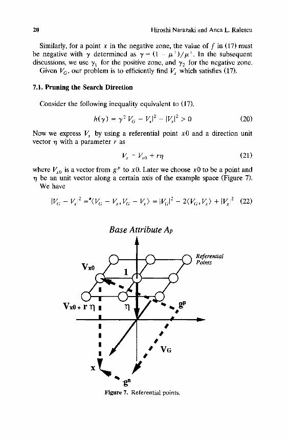
Now we express V~ by using a referential point x0 and a direction unit vector 77 with a parameter r as
V~ = Vx0 + rr/ (21)
where Vx0 is a vector from gP to x0. Later we choose x0 to be a point and "q be an unit vector along a certain axis of the example space (Figure 7).
We have
I V G - V~I 2 = ° ( V a - V~, V a - V x ) = [VGI 2 -- 2 ( V G , V~) + IVxl 2 (22)
Base Attribute At,
Referent ia l Points
Vxo+ r n , n ..ff
! I
i S
,g. Figure 7. Referential points.
Alternative Method for Inducing a Membership Function 21
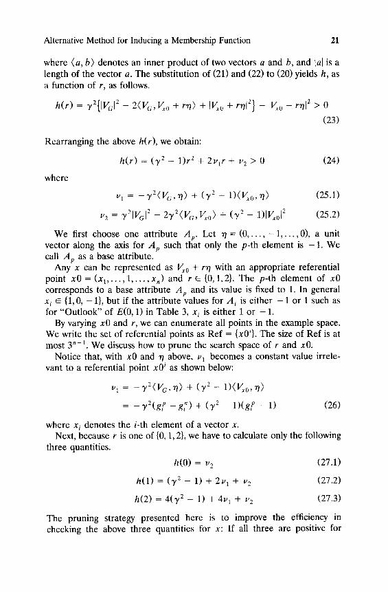
where ( a , b ) denotes an inner p roduc t of two vectors a and b, and lal is a length of the vec tor a. The subst i tut ion of (21) and (22) to (20) yields h, as a funct ion of r, as follows.
h(r) = y2{[VGI2 - 2 ( V G, V.o + rrl) + tV~o + rrlJ 2} - [Vxo + rr/[ 2 > 0
(23)
Rear rang ing the above h(r), we obtain:
h(r) = ( , y 2 _ 1)r 2 + 2ulr + u2 > 0
where
P2
(24)
Pl = - - ' y 2 ( V G , TI) q- ( ] / 2 _ 1 ) ( V x o , g l ) ( 2 5 . 1 )
= ~,21vcl 2 _ 2,y2(VG, Vxo) q._ ( , y 2 _ 1)[V~o[2 ( 2 5 . 2 )
W e first choose one at t r ibute Ap. Let r / = (0 . . . . . - 1 . . . . . 0), a unit vector along the axis for A v such that only the p - th e lement is - 1 . We call Ap as a base at tr ibute.
Any x can be r ep resen ted as Vx0 + r'q with an appropr ia t e referent ia l point x0 = (x 1 . . . . . 1 . . . . . x , ) and r ~ {0, 1,2}. The p - th e l emen t of x0 cor responds to a base a t t r ibute Ap and its value is fixed to 1. In general x i ~ {1, 0, - 1}, but if the a t t r ibute values for A i is e i ther - 1 or 1 such as for " O u t l o o k " of E(0, 1) in Table 3, xi is e i ther 1 or - 1.
By varying x0 and r, we can e n u m e r a t e all points in the example space. We write the set of referent ia l points as R e f = {x0i}. The size of R e f is at most 3 n- 1. W e discuss how to prune the search space of r and x0.
Notice that, with x0 and ~ above, v 1 becomes a constant value irrele- vant to a referent ia l point x0 i as shown below:
1~ l = _ _ , ~ 2 ( V G , n ) + ( ~ 2 __ 1)(V~o,~ )
= - T 2 ( g f - g ~ ) + (3, 2 - 1)(gi p - 1) (26)
where x i denotes the i-th e lement of a vector x. Next, because r is one of {0, 1, 2}, we have to calculate only the following
three quantit ies.
h(0) = v 2 (27.1)
h(1) = (72 _ 1) + 2v 1 + v 2 (27.2)
h(2) = 4 ( ' y 2 - 1 ) + 4 v 1 + v 2 (27.3)
The pruning strategy p resen ted here is to improve the efficiency in checking the above three quanti t ies for x: I f all three are positive for
22 Hiroshi Narazaki and Anca L. Ralescu
]/ = "Yl, then x is in the positive zone. In contrast, if they are all negative for 3' = 3'2, then x is in the negative zone.
Since
h(1) - h(0) = 3, 2 - 1 + 2v 1 (28.1)
h(2) - h ( l ) = 3 ( T 2 - 1) + 2v 1 (28.2)
h(2) - h(0) = 4(y 2 - 1) + 4v 1 (28.3)
it follows that the order of h(0), h(1) and h(2) is predetermined, indepen- dent of the referential point xO i ~ Ref. For example, suppose that for given 3' and Vl, h(1) - h(0) < 0, h(2) - h(1) < 0. Then h(0) > h(1) > h(2), and if h(0) < 0 at a certain referential point, then we find that h(1), h(2) < 0 at that referential point without actually calculating them.
Therefore the following pruning strategy can be used: 1. For given y and v 1, determine the order of h(0), h(2), and h(3) from
(28.1), (28.2) and (28.3). Let the ordered values of h(0), h(1), and h(2) be h(o ) > h(1 ) >_ h(2).
2. At this stage, only the order is determined, but the values of h(o ), ho), and h(2 ) are not yet known. For each referential point xO i ~ Ref, we calculate those values as follows: Step 1: Calculate h(2 ). If h(2 ) > 0, then h(0 ), h(1 ) > 0. Step 2: Calculate h(0 ). If h(0 ) < 0, then h(1), h(2 ) < 0. Step 3: Calculate h(1 ). A t this stage, we know all the three quantities,
h(0), h(1), and h(2).
Steps 1 and 2 can be performed in reverse order. A heuristic strategy can be used to choose this order: If [Ix0 i -gP l l < 11 x0i - g " ] [ , then start with step 1, else start with step 2.
7.2. Pruning of Referential Points
Next we discuss the pruning strategy for Ref. Let x01 and x0 2 be two referential points in Ref. For simplicity, we define that the inequality of vectors is judged by elementwise comparisons, i.e., 7
xO' <_ xO 2 xO] <_ xO] vj( p)
If x01 < (or >)x02, we say that x01 is smaller (or larger) than X0 2. We establish our pruning strategy for referential points based on v2: From (27.1)-(27.3), if v 2 is monotone nondecreasing, then so is h(r ) for any r ~ {0, 1,2}. In other words, if h ( r ) > O, Vr ~ {0, 1, 2}, at a referential
7 We need not consider the base attribute.
Alternative Method for Inducing a Membership Function 23
point x01, then, for any referential point X0 2 >__ X01, we have also h(r) > 0, Vr ~ {0, 1, 2}.
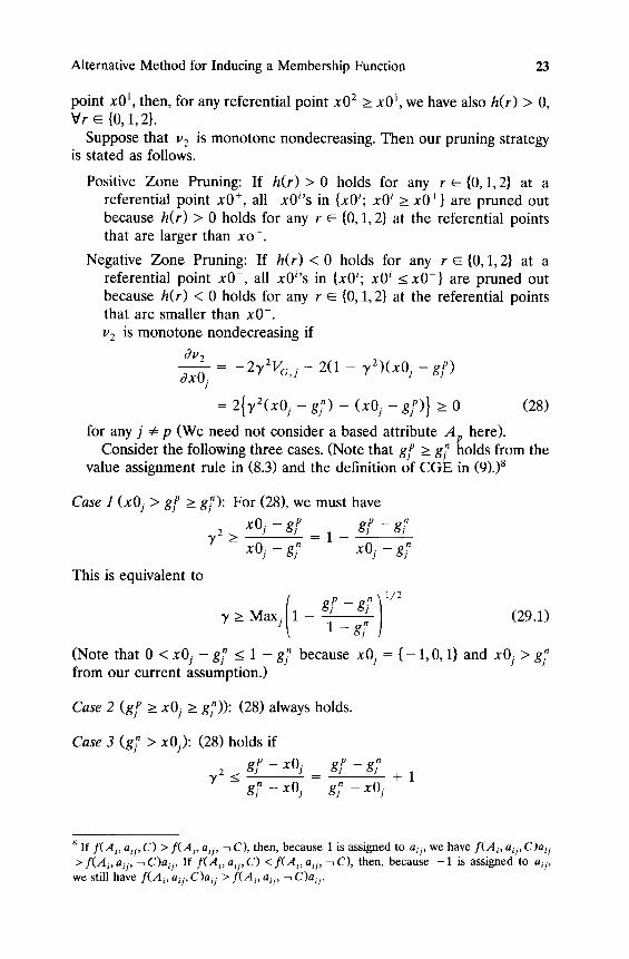
Suppose that P2 is monotone nondecreasing. Then our pruning strategy is stated as follows.
Positive Zone Pruning: If h( r )> 0 holds for any r ~ {0, 1,2} at a referential point x0 +, all xOi's in {x0i; x0 i > x0 ÷} are pruned out because h(r) > 0 holds for any r ~ {0, 1, 2} at the referential points that are larger than xo +.
Negative Zone Pruning: If h ( r ) < 0 holds for any r ~ {0, 1,2} at a referential point x0- , all x0i's in {x0i; x0 i < x0 } are pruned out because h(r) < 0 holds for any r ~ {0, 1, 2} at the referential points that are smaller than x0- . v 2 is monotone nondecreasing if
Ov 2 - 2TzVG.j -- 2(1 -- 3'2)(x0j --gP)
OxOj
= 2{3"2(xOj - -g ; ) -- (xOj --uP)} > 0 (28)
for any j 4= p (We need not consider a based attribute Ap here). Consider the following three cases. (Note that g f > g ; holds from the
value assignment rule in (8.3) and the definition of CGE in (9).) 8
Case 1 (xO~ > g f > g~): For (28), we must have x0j - gP gP - g ;
3'2 > 1 - g ; xOj - g ;
This is equivalent to n ) 1/2
3' > Maxj 1 gP - g) - 1 - g ~
(Note that 0 < xOj - g7 < 1 - g~ because xOj from our current assumption.)
(29.1)
= { -1 , 0, 1} and xOj > g7
Case 2 (gP > xOj > g;)): (28) always holds.
Case 3 (g7 > x0/): (28) holds if
gf -x0j 3"2<
g; - x O j g f - g ? g7 - xOj
+ 1
8 If f ( A i , aij , C) > f ( a i , aij, ~ C), then, because 1 is assigned to aij, we have f ( A i , aij , C)ai j > f ( A i , aij , ~ C)ai j . If f ( a i , aij , C) < f ( A i , aij, ~ C), then, because - 1 is assigned to aij, we still have f ( a i , aij , C)ai j > f ( A i , aij, -1 C)aij .
24 Hiroshi Narazaki and Anca L. Ralescu
This is equivalent to
y < M i n j 1 + ~ + ] - (29.2)
(Again, note that - 1 - g7 < x0j - g7 < 0, and thus 1 + g ; > g ; - x0j > 0).
In summary, we have the following lemma.
LEMMA (CONDITION FOR MONOTONICITY OF ~'2) Assume that we choose Ap as a base attribute. Forgiven gP, gn, and y, if
Maxj ,p 1 l - - g 7 _< y < M i n j . p 1 + g f - g ; 1/2 g; (30)
holds, then v 2 is monotone nondecreasing.
We choose Ap such that (30) holds.
7.3. Summary
Our pruning strategies are summarized as follows. We denote a set of expressions of the positive examples by S.
Ordering h(r): First choose a base attribute and determine the order of h(r)'s. Here we assume h(0) > h(1) > h(2).
Positive Zone Pruning: Calculate h(r)'s based on Yl, the value of y for the positive zone. If h (2 )> 0 (i.e., all are positive), then all the referential points in {x0i; x 0 i > x01} are in the positive zone and pruned out from Ref.
Negative Zone Pruning: Calculate h(r)'s based on 3'2, the value of 3' for the negative zone. If h ( 0 ) < 0 (i.e., all are negative), then all the referential points in {x0~; x0 ~ < x01} are in the negative zone and pruned out from Ref.
Fuzzy Zone Search: Points are not in the fuzzy zone or negative zone. For these points we generate the corresponding expressions and the classification test is done for them.
A good heuristic for referential point search is to start from the point nearest to gP by increasing the number of l 's step by step. For example, we scan all referential points having only one element with the value "1," and we move to the referential points having two l's. If we find a point where all h(r)'s are positive, we can prune all referential points larger than
Alternative Method for Inducing a Membership Function 25
that. Similar search can be applied to the negative zone, by increasing the number of - 1 step by step.
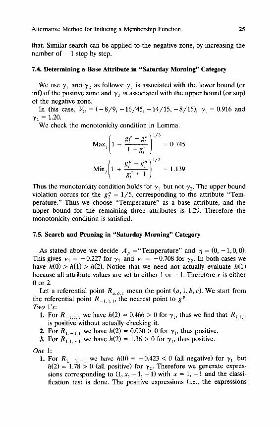
7.4. Determining a Base Attribute in "Saturday Morning" Category
We use Yl and 72 as follows: 71 is associated with the lower bound (or inf) of the positive zone and Y2 is associated with the upper bound (or sup) of the negative zone.
In this case, V c = ( - 8 / 9 , - 16/45, - 14/15, - 8 / 1 5 ) , )'1 = 0.916 and Y2 = 1.20.
We check the monotonicity condition in Lemma.
Maxj (1
Mini (1 + m
g f -- g7 ]1/2 0.745
1 - g ; J n ) 1/2 g f - gj
g? + i = 1.139
Thus the monotonicity condition holds for 71 but not 72. The upper bound violation occurs for the g~' = 1/5, corresponding to the attribute "Tem- perature." Thus we choose "Tempera ture" as a base attribute, and the upper bound for the remaining three attributes is 1.29. Therefore the monotonicity condition is satisfied.
7.5. Search and Pruning in "Saturday Morning" Category
As stated above we decide Ap ="Tempera tu re" and "q = (0, - 1 , 0, 0). This gives ~'1 = -0 .227 for 7~ and v 1 = -0 .708 for T2. In both cases we have h(0) > h(1) > h(2). Notice that we need not actually evaluate h(1) because all attribute values are set to either 1 or - 1. Therefore r is either 0 o r 2 .
Let a referential point Ra, b, c mean the point (a, 1, b, c). We start from the referential point R_1,1,1, the nearest point to gP. Two l 's:
1. For R1,1,1 we have h(2) = 0.466 > 0 for Yl, thus we find that RLL 1 is positive without actually checking it.
2. For R1,_ 1,1 we have h(2) = 0.030 > 0 for 71, thus positive. 3. For R1,1,- 1 we have h(2) = 1.36 > 0 for 71, thus positive.
One 1: 1. For R1. 1,- 1 we have h(0) = -0 .423 < 0 (all negative) for Yl but
h(2) = 1.78 > 0 (all positive) for ~/2. Therefore we generate expres- sions corresponding to (1, x, - 1, - 1) with x = 1, - 1 and the classi- fication test is done. The positive expressions (i.e., the expressions
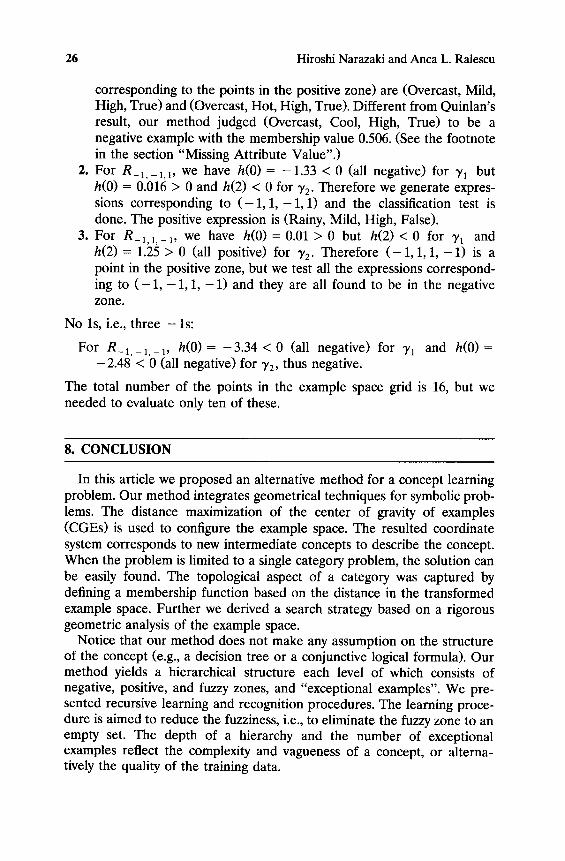
26 Hiroshi Narazaki and Anca L. Ralescu
corresponding to the points in the positive zone) are (Overcast, Mild, High, True) and (Overcast, Hot, High, True). Different from Quinlan's result, our method judged (Overcast, Cool, High, True) to be a negative example with the membership value 0.506. (See the footnote in the section "Missing Attribute Value".)
2. For R_I._ 1,1, we have h(0) = -1.33 < 0 (all negative) for 3'1 but h(0) = 0.016 > 0 and h(2) < 0 for 3'2. Therefore we generate expres- sions corresponding to ( - 1 , 1 , - 1, 1) and the classification test is done. The positive expression is (Rainy, Mild, High, False).
3. For R_1,1,_1, we have h ( 0 ) = 0 . 0 1 > 0 but h ( 2 ) < 0 for 3'x and h(2) = 1.25 > 0 (all positive) for 3'2. Therefore ( - 1 , 1, 1 , - 1) is a point in the positive zone, but we test all the expressions correspond- ing to ( - 1, - 1 , 1, - 1 ) and they are all found to be in the negative zone.
No ls, i.e., three - l s :
For R1,_1._1, h (0)= -3.34 < 0 (all negative) for 3'1 and h(0)= - 2 . 48 < 0 (all negative) for 3'2, thus negative.
The total number of the points in the example space grid is 16, but we needed to evaluate only ten of these.
8. CONCLUSION
In this article we proposed an altemative method for a concept learning problem. Our method integrates geometrical techniques for symbolic prob- lems. The distance maximization of the center of gravity of examples (CGEs) is used to configure the example space. The resulted coordinate system corresponds to new intermediate concepts to describe the concept. When the problem is limited to a single category problem, the solution can be easily found. The topological aspect of a category was captured by defining a membership function based on the distance in the transformed example space. Further we derived a search strategy based on a rigorous geometric analysis of the example space.
Notice that our method does not make any assumption on the structure of the concept (e.g., a decision tree or a conjunctive logical formula). Our method yields a hierarchical structure each level of which consists of negative, positive, and fuzzy zones, and "exceptional examples". We pre- sented recursive learning and recognition procedures. The learning proce- dure is aimed to reduce the fuzziness, i.e., to eliminate the fuzzy zone to an empty set. The depth of a hierarchy and the number of exceptional examples reflect the complexity and vagueness of a concept, or alterna- tively the quality of the training data.
Alternative Method for Inducing a Membership Function 27
Further we pointed out that our learning algorithm for the single category problem does not include any heuristic search, and the computa- tional cost is proportional to the number of examples multiplied by the depth of the hierarchy. However, the search for the symbolic description of the learned knowledge still requires computation of exponential order. This suggests that in application we can have a simpler method for the classification task than the traditional inductive learning based on the heuristic search. To improve the explanatory capability of the learning system, the problem of approximate symbolic description search as a trade-off between the search time and the precision of the generated symbolic expression is our future work.
References
1. Quinlan, J. R., Learning efficient classification procedures and their applica- tion to chess and games, in Machine Learning: An Artificial Intelligence Ap- proach, (Michaslski, Carbonell, and Mitchell, Eds.), Morgan Kaufmann, CA, 1983.
2. Quinlan, J. R., Induction of decision trees, Machine Learning 1, 81-106, 1986.
3. Cheng, J., Fayaad, U. M., Irani, K. B., Quian, Z., Improved decision trees: A generalized version of ID3, Proc. of 5th Int. Conf. on Machine Learning Ann Arbor, MI, 100-106, 1988.
4. Michalski, R. S., A theory and methodology of inductive learning, in Machine Learning: An Artificial Intelligence Approach (Michaslski, Carbonell, and Mitchell, Eds.), Morgan Kaufmann, CA, 1983.
5. Mitchel, T. M., Generalization as search, Artificial Intelligence 18, 203-226, 1982.
6. Mitchell, T. M., The need for biases in learning generalizations, Technical Report No. CBM-TR-117, Rutgers University, Department of Computer Sci- ence, New Brunswick, NJ, 1980.
7. Miyamoto, S., Fuzzy Sets in Information Retrieval and Cluster Analysis, Kluwer Academic Publishers, 1990.
8. Snedecor, G. W., and Cochran, W. G., Statistical Methods, 6th edition, Iowa State University Press, Iowa, 1967.
9. Nillson, N., Learning Machines, McGraw-Hill, New York, 1965.
10. Minsky, M. L., and Papert, S., Perceptrons: An Introduction to Computational Geometry, MIT Press, Cambridge, MA, 1969.
1l. Ullman, J. R., Pattern Recognition Techniques, Butterworth &Co., London, 1973.
28 Hiroshi Narazaki and Anca L. Ralescu
12. Rumelhart, D. E., McClelland, J. L., and the PDP Research Group (Eds.), Parallel Distributed Processing (Vol. 1, Vol. 2) MIT Press, Cambridge, MA, 1986.
13. Weiss, S. M., and Kapouleas, I., An empirical comparison of pattern recogni- tion, neural nets, and machine learning classification methods, Proc. of the 11th IJCAI 781-787, Detroit, 1989.
14. Way, E. C., Conceptual graphs, family resemblances and open texture, Proc. of the 4th Annual Workshop on Conceptual Graphs Detroit, 1989.
15. Ralescu, A. L., and Baldwin, J. F., Concept learning from examples and counter examples, Int. J. Man-Machine Syst. 30(3), 1989.
16. Berenji, H. R., and Khedkar, P., Learning and tuning fuzzy logic controllers through reinforcements, IEEE Trans. on NN 3(3), 1992.