An AI Method to Score Charisma from Human Faces

Xiaohang Feng

PhD Student, Tepper School University, Carnegie Mellon University

4765 Forbes Ave, Pittsburgh, PA 15213

+1 (412) 214-2446, xiaohanf@andrew.cmu.edu

Shunyuan Zhang Assistant Professor, Harvard Business School, Harvard University

Soldiers Field, Boston, MA 02163

+1 (617) 495-4903, szhang@hbs.edu

Xiao Liu Associate Professor, Stern School of Business, New York University

44 West 4th Street, New York, NY 10012

+1 (212) 998-0406, xl23@stern.nyu.edu

Kannan Srinivasan H.J. Heinz II Professor, Tepper School University, Carnegie Mellon University

4765 Forbes Ave, Pittsburgh, PA 15213

+1 (412) 268-8840, kannans@cmu.edu

An AI Method to Score Charisma from Human Faces

Abstract

Charismatic individuals such as business leaders, politicians, and celebrities have extraordinary

abilities to attract and influence others. Predicting charisma is important in the domains of

business, politics, media, and entertainment. Can we use human faces to predict charisma? If so,

which facial features have the most impact on charisma? We develop a three-step empirical

framework that leverages computer vision techniques to predict charisma from face images. In

the prediction step, we optimize a ResNet-50 deep learning model on a large dataset of 6,000

celebrity images and 6,000 non-celebrity images and achieve 95.92% accuracy. In the

interpretation step, we draw on psychology, economics, and behavioral marketing literature to

select 11 interpretable facial features (e.g., width-to-height ratio). We calculate the direction and

strength of the feature’s correlation with charisma. We find that the facial width-to-height ratio,

babyfaceness, and thin jaw contribute negatively to charisma while sexual dimorphism, dark skin

color, and large eyes contribute positively. In the mechanism step, we compare the interpretation

results with extant theoretical relationships between facial features and charisma, with

personality traits as mediators. Contradicting theoretical predictions, we discover a negative

correlation between averageness and charisma. We demonstrate the generalizability of our results

to media/entertainment and business domains.

Keywords: Charisma Classification, Facial Features, Personality Traits, Deep Learning, XAI.

INTRODUCTION

Charisma refers to an inner quality that distinguishes an individual from ordinary people and can

elicit devotion from others.1 It is one of the most prominent individual characteristics in business,

politics, and media and is a crucial quality indicator, especially among leaders (Conger et al.

2000; Dvir et al. 2002; Kanter 2012). Charismatic individuals include heroic generals, political

revolutionaries, C-suite executives, and influential celebrities—their excellence at capturing

attention and social networking enables success in diverse contexts (Antonakis et al. 2016;

Friedman et al. 1980; King 2015). Therefore, predicting charisma is of great importance for

decision making in the domains of business, politics, media, and entertainment. For example, an

accurate prediction of charisma could help talent agency companies analyze who to invest, aid

human resources executives to judge whether an interviewee is well-suited for a managerial

position, and forecast election results.

Charisma is a broad concept and can be explained by combinations of traits such as success,

popularity, and attractiveness, but it differs from each individual trait. For instance, success can

be measured by income or company hierarchy, which leads to individual identity and satisfaction

(Goffman 1961; Arthur et al. 2005), but success differs from charisma, which emphasizes

interpersonal influence. Popularity overlaps with charisma in terms of social acceptance and the

quality of being well-liked (Eder 1985), but charisma, unlike popularity, includes the ability to

elicit trust and respect from others. Attractiveness involves external, short-term physical charm

(Swami and Furnham 2008), while charisma extends to a multi-faceted, long-term influence on

the perceiver’s mind and emotions (Chase 2016).

1 The widely accepted definition treats charisma as a personality trait that differentiates someone from ordinary people; a charismatic person is perceived to have exceptional powers and qualities that elicit devotion from others (Weber 1947; Joosse 2014).

Charisma is a comprehensive quality that can be judged from both (inner) personality traits

and (outer) physical appearance. Extant research, however, focuses disproportionately on how

charisma relates to various personality traits (e.g., warmth, dominance). By contrast, the present

research evaluates how charisma relates to facial features. Faces are important visual stimuli that

convey rich social information such as underlying emotions, personality traits, and leadership

abilities. Facial features have been shown to influence critical outcomes including organizational

performance (Rule and Ambady 2008; Wong et al. 2011), election results (Tanner and Maeng

2012; Todorov et al. 2005), networking (Li and Xie 2020), relationship formation (Todorov and

Porter 2014), and marketing efficiency (Ordenes et al. 2018). Facial features influence observers’

perceptions of individual characteristics that are key to outcomes in many contexts. For example,

facial expressions can affect interpersonal perceptions of warmth and competence, which

influence consumer choices (Zhang et al. 2020).

Given ample evidence that a person’s face contains morphological and social cues that

inform perceptions of personality, we hypothesize that facial features can predict charisma—a

topic that is not yet studied. We ask three questions: 1) Can we develop a high-performing,

generalizable, and scalable model that extracts facial attributes from a photo and quantifies the

person’s charisma? 2) Which facial attributes contribute the most to charisma? 3) Can our model,

implemented on large-scale empirical data, add clarity to existing theories about the relationships

between facial attributes and charisma, with personality traits as mediators?

We answer these questions in a three-step research framework. In the prediction step, we

constructed a unique dataset of 722,418 celebrity images and 158,611 non-celebrity images. We

randomly selected 12,000 images for training and 10,000 for testing. We used the “celebrity”

label as a proxy for charisma because previous research suggests that “celebrity icons” possess a

charismatic power that transcends time and space (Alexander 2010; Marshall 1997; Rojek 2001;

Berenson and Giloi 2010; Friedman et al. 1988; Friedman et al. 1980). We employed deep

learning techniques to build a model that discriminates between celebrity and non-celebrity

faces; the model’s output is the probability that the inputted face was a celebrity. We refer to this

probability as the charisma score. We fine-tuned our model architecture with pre-processing

techniques to avoid overfitting and to minimize systematic differences (e.g., illumination, face

rotation/alignment) among photos taken under various conditions (Kazemi and Sullivan 2014;

Zhang et al. 2007).

In the interpretation step, we measured the direction and ranked the strength of the

correlation between charisma and each of the 11 facial features that we identified as relevant in

the literature on charisma. To establish the direction of each correlation for each facial feature,

we constructed (through selection or manipulation) two groups of images that varied

dramatically on the focal feature. Then, we tested the variation in the charisma score between the

two contrasting groups. We also connected the 11 facial features with the 50 nodes in the

customized dense layer of the deep learning model by using the contrasting groups of images to

identify the most active nodes for each facial feature. We ranked the contributions of the facial

features based on the weighted contributions of the nodes with the SHapley Additive

exPlanations (SHAP) algorithm (Lundberg and Lee 2017), an advanced Explainable Artificial

Intelligence (XAI) method. To achieve computational efficiency on our large set of face images,

we built a new tree model on top of the 50-node dense layer in the deep learning model

(Lundberg et al. 2020), and we obtained the mean SHAP value for each node across the 10,000

images. We derived a charisma formula that quantifies the contribution of each facial feature

based on the SHAP values and connections between facial features and nodes. We also examined

individual heterogeneity in the contribution and ranking of the facial features.

In the mechanism step, we drew upon theories from psychology, consumer behavior, and

economics to identify six personality traits2 (e.g., trustworthiness, aggressiveness) that mediate

the connection between the 11 facial features and charisma (Gray et al. 2014; Keating 2002

2011). Most facial features affect multiple personality traits, creating theoretically composite

effects on charisma (i.e., charisma should be increased by the feature’s effect on one trait but

decreased by the feature’s effect on another trait). We compared the theoretical and empirical

correlations between facial features and charisma to test previous theories and to clarify the

direction of the effects for features with theoretical trade-offs among multiple personality traits.

Finally, we tested whether our model generalizes to two other contexts: media/entertainment

and business. For the media/entertainment context, we collected selfie posts from Instagram

influencers to test the correlation between the charisma score and the number of followers,

controlling for the effects of post popularity, facial beauty, text features, and basic demographic

information. We also compared the charisma scores of Instagram influencers with average

Instagram users. For the business context, we used profile images crawled from LinkedIn to

compare the mean charisma scores of C-suite executives with those of average employees. For

both datasets, we used SHAP values to examine individual heterogeneity in the contributions of

each facial feature to the individual’s charisma.

We report four main results. First, we successfully constructed a deep learning model that

predicts charisma from face images, achieving 95.92% accuracy on a hold-out test set. Second, at

2 A “personality trait” is an internal characteristic (Cattell 1950). We don’t count physical attractiveness as one, though it may mediate the relationships between facial features and charisma (Berscheid and Walster 1978; Griffin and Langlois 2006).

the population level, we reveal that charisma correlates negatively with the facial width-to-height

ratio, babyfaceness, thin jaw, etc.; charisma correlates positively with sexual dimorphism, dark

skin color, large eyes, etc. At the population level, the five features that correlate most strongly

with charisma are, in descending order, the facial width-to-height ratio, sexual dimorphism,

averageness, high cheekbones, and skin color. There is also individual heterogeneity in the

contribution of each facial feature to charisma. Third, while most empirical results align with the

theoretical predictions, we discovered a negative correlation between charisma and averageness

that contradicts the results from our survey of the literature. We also clarified the outcomes of

several theoretical trade-offs among personality traits that mediate the relationship between the

facial features and charisma. Finally, the charisma score showed high validity in analyses of two

alternative datasets (influencers vs. average users on Instagram; C-suite executives vs. average

employees on LinkedIn).

We offer two main theoretical contributions. First, to the best of our knowledge, this

research is the first to directly predict charisma from extracted facial features. Second, we

comprehensively consolidate prior knowledge on the relationship between charisma and the 11

facial features. Although various facial attributes and personality traits have been studied in

marketing and economics (e.g., warmth: Livingston and Pearce 2009; trustworthiness: Hoegg

and Lewis 2011), most studies have small samples and use human judgment to rate the

personality traits. We make a methodological contribution by developing a classification model

that can predict a person’s charisma based on their face image, handle a large volume of data,

and characterize the relationship between facial features and charisma.3

3 Our nonparametric deep learning model is more robust than parametric regression models because it can achieve much higher accuracy without restricting the function form of the relationship between the facial attributes and charisma.

Finally, our work provides significant managerial implications for marketing, media,

entertainment, politics, and business. The charisma score may be a useful tool for screening

human photos that are intended to sway an audience (e.g., in advertisements). Moreover, our

work highlights heterogeneity in the contribution of facial features to charisma. A talent agency

company could apply our model to optimize the charisma (e.g., through make-up and/or

hairstyle) of each individual. Our findings have similar applications for investing in social media

influencers to promote a firm’s products and anticipating the suitability of a candidate for an

executive position.

LITERATURE REVIEW

Our paper is related to two strands of literature: the relationship between facial features and

charisma-related personality traits, and facial feature analytics in marketing.

Relationship Between Facial Features And Charisma-Related Personality Traits

Charisma encompasses a leader’s moral conviction, need for power, and ability to transfer an

idealized vision to followers. It can be explained through a combination of personality traits

including (i) a sense of power/dominance, (ii) trustworthiness, (iii) competence, (iv)

aggressiveness, (v) warmth, and (vi) generosity, as well as (vii) physical attractiveness (House

and Howell 1992; House et al. 1991). Specifically, charisma is positively associated with

dominance, which elicits avoidance behavior (Keating 2002); warmth, which leads to approach

behaviors among followers (Keating 2011); generosity, which is regarded as an important virtue

for good leadership and social recognition (Winterich, Mittal, and Aquino 2013; Beck 2012); and

competence, which elicits positive emotions among followers (Avolio and Bass 1988; Bass

1985; Gray et al. 2014; Yukl 1999). By contrast, aggressiveness decreases charisma by reducing

one’s ability to arouse positive emotions in other people (Buss and Perry 1992; Costa et al.

1988). In addition, the existing literature has diverging conclusions on the impact of physical

attractiveness on charisma; for example, Riggio (1987) argues that the effect is small, while

others believe that attractiveness influences first impressions and correlates with positive

qualities (Berscheid and Walster 1978; Griffin and Langlois 2006)

Previous studies have shown that the six charisma-related personality traits can be inferred

from one’s facial features. From an exhaustive review of the literature in psychology, economics,

and behavioral marketing, we identified 11 facial features that are relevant to charisma. We

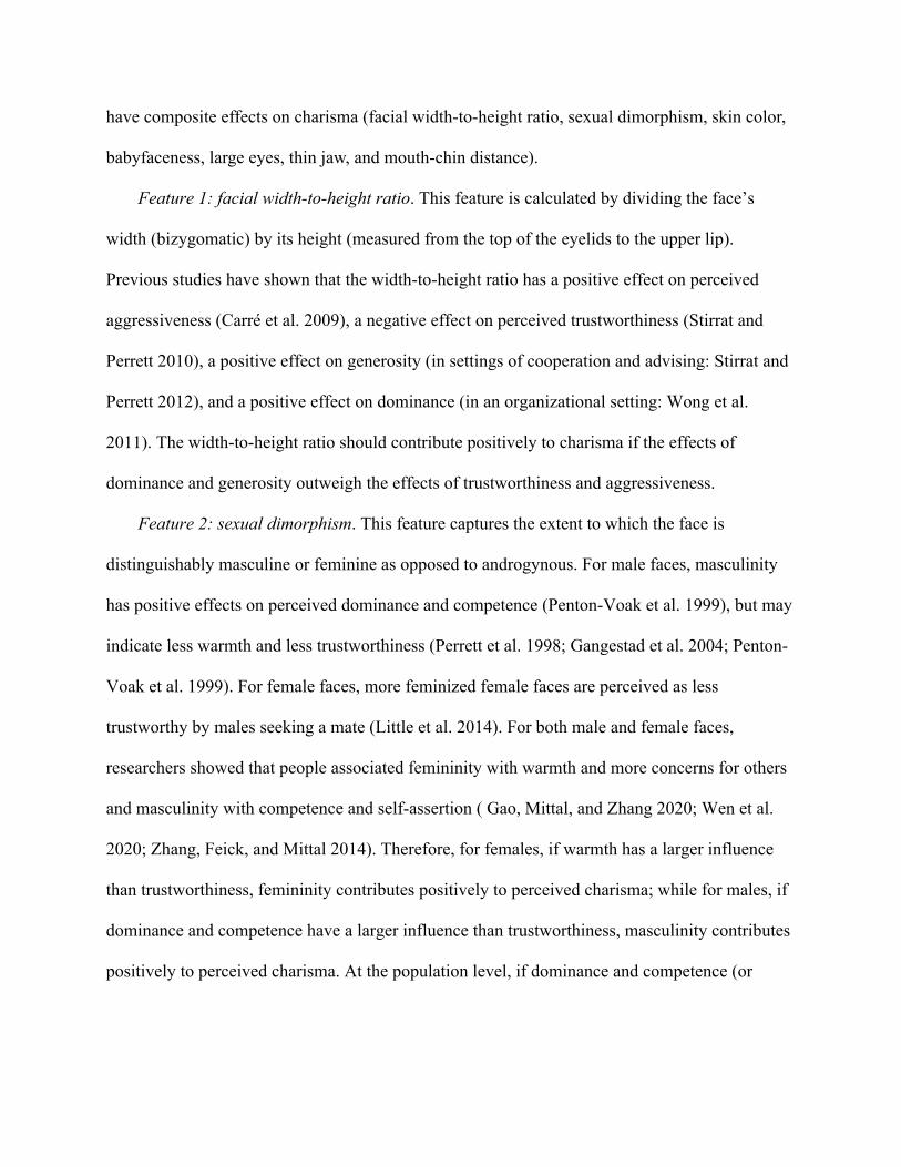
depict the theoretical relationship between charisma and the 11 facial features, with the six

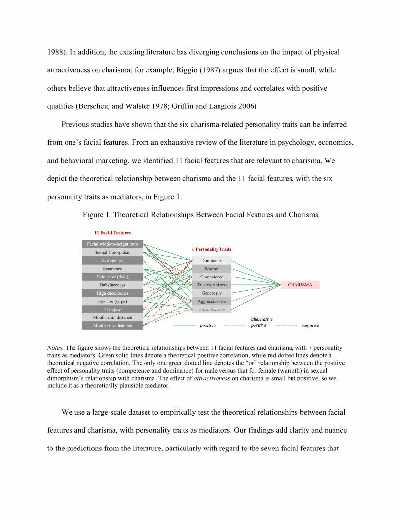
personality traits as mediators, in Figure 1.

Figure 1. Theoretical Relationships Between Facial Features and Charisma

Notes. The figure shows the theoretical relationships between 11 facial features and charisma, with 7 personality traits as mediators. Green solid lines denote a theoretical positive correlation, while red dotted lines denote a theoretical negative correlation. The only one green dotted line denotes the “or” relationship between the positive effect of personality traits (competence and dominance) for male versus that for female (warmth) in sexual dimorphism’s relationship with charisma. The effect of attractiveness on charisma is small but positive, so we include it as a theoretically plausible mediator.

We use a large-scale dataset to empirically test the theoretical relationships between facial

features and charisma, with personality traits as mediators. Our findings add clarity and nuance

to the predictions from the literature, particularly with regard to the seven facial features that

have composite effects on charisma (facial width-to-height ratio, sexual dimorphism, skin color,

babyfaceness, large eyes, thin jaw, and mouth-chin distance).

Feature 1: facial width-to-height ratio. This feature is calculated by dividing the face’s

width (bizygomatic) by its height (measured from the top of the eyelids to the upper lip).

Previous studies have shown that the width-to-height ratio has a positive effect on perceived

aggressiveness (Carré et al. 2009), a negative effect on perceived trustworthiness (Stirrat and

Perrett 2010), a positive effect on generosity (in settings of cooperation and advising: Stirrat and

Perrett 2012), and a positive effect on dominance (in an organizational setting: Wong et al.

2011). The width-to-height ratio should contribute positively to charisma if the effects of

dominance and generosity outweigh the effects of trustworthiness and aggressiveness.

Feature 2: sexual dimorphism. This feature captures the extent to which the face is

distinguishably masculine or feminine as opposed to androgynous. For male faces, masculinity

has positive effects on perceived dominance and competence (Penton-Voak et al. 1999), but may

indicate less warmth and less trustworthiness (Perrett et al. 1998; Gangestad et al. 2004; Penton-

Voak et al. 1999). For female faces, more feminized female faces are perceived as less

trustworthy by males seeking a mate (Little et al. 2014). For both male and female faces,

researchers showed that people associated femininity with warmth and more concerns for others

and masculinity with competence and self-assertion ( Gao, Mittal, and Zhang 2020; Wen et al.

2020; Zhang, Feick, and Mittal 2014). Therefore, for females, if warmth has a larger influence

than trustworthiness, femininity contributes positively to perceived charisma; while for males, if

dominance and competence have a larger influence than trustworthiness, masculinity contributes

positively to perceived charisma. At the population level, if dominance and competence (or

warmth) have (has) a larger influence than trustworthiness, sexual dimorphism (i.e., masculinity

or femininity) contributes positively to perceived charisma.

Feature 3: averageness. Averageness is the extent to which the face’s features align with the

average features of all people of the same gender, race, and approximately the same age.

Averaged faces are perceived as more attractive (Rhodes and Tremewan 1996), likely because

evolutionary pressures favor characteristics close to the mean of the population (Langlois and

Roggman 1990). Given that physical attractiveness has a positive correlation with charisma, we

anticipated a positive effect of averageness on charisma.

Feature 4: symmetry. Facial symmetry is the visual similarity (in shape and color) between

the left and right sides of the face. Symmetry has positive effects on perceived attractiveness

(Alley and Cunningham 1991; Gangestad et al. 2004; Rhodes et al. 1999), competence (in social

networking: Pound et al. 2007; Fink et al. 2005; Fink et al. 2006), and conscientiousness and

trustworthiness (Noor and Evans 2003). Attractiveness, competence, and trustworthiness all

contribute positively to charisma, so we anticipated that facial symmetry also has a positive

correlation with charisma.

Feature 5: color. Color is the skin tone of the face. Darker skin color is perceived as more

dominant and high status, especially for athletes and entertainers (Wade 1996; Wade and Bielitz

2005), but may be perceived as more aggressive as well (Eberhardt et al. 2006, Livingston and

Pearce 2009). Darker skin color should contribute positively to charisma if its effect on

dominance outweighs its effect on aggressiveness.

Feature 6: babyfaceness. Babyfaceness is the extent to which the face’s features resemble a

typical baby’s rather than a typical adult’s. The defining characteristics are large eyes, a small

nose, a high forehead, and a small chin. Babyfaceness has positive correlations with perceived

honesty and warmth (Gorn et al. 2008) and negative correlations with perceived power,

dominance, and aggressiveness (Livingston and Pearce 2009; Zebrowitz and Montepare 2005).

Babyfaceness should have a positive correlation with charisma if its effects on warmth,

trustworthiness, and aggressiveness outweigh its effect on dominance.

Feature 7: thin jaw. Jaw width is calculated as the distance between the two edges of a jaw.

A broader jaw has positive correlations with dominance and strength (Cunningham et al. 1990;

Keating et al. 1981) as well as aggressiveness (Tˇrebický et al. 2013). A thin jaw correlate

negatively with charisma if its effect on dominance outweighs its effect on aggressiveness.

Feature 8: large eyes. Eye size means the relative size of an eye against the whole face.

Large eyes are perceived as more attractive (specifically, the perception that one is “charming”;

Alley and Cunningham 1991). They also heighten perceptions of warmth, trust, and

submissiveness (the opposite of perceived dominance; Keating 1985; Montepare and Zebrowitz

1998; Zebrowitz 1997). Thus, if the total positive mediating effect of warmth, trust, and

attractiveness outweigh the negative mediating effect of dominance, we can conjecture that

(large) eye size correlates positively with charisma.

Feature 9: high cheekbones. The cheekbones, particularly the malar bones, support facial

structure; a person has “high cheekbones” if their malar bones are located closer to the eyes. In

males, high cheekbones have positive effects on perceived competence and dominance (in social

networking: Cunningham et al. 1990). Females with low cheekbones are perceived as less

competent (in reproductivity and social networking: Cunningham 1986). Thus, high cheekbones

are positively related to competence, so we predicted a positive correlation with charisma.

Feature 10: mouth-nose distance. This is the vertical distance between the nose tip and the

upper lip. Researchers have found that attractive faces usually have a shorter mouth-nose

distance (Perrett et al. 1994) and that a longer mouth-nose distance may predict sarcasm (Tay

2014), which is a passive, verbal form of aggressiveness (Pickering et al. 2018; Szymaniak and

Kałowski 2020). Also, people with a short mouth-nose distance are perceived as more focused

and flawless, so they likely are perceived as more competent (Stevens 2011; Dunn 2018). The

effects of the mouth-nose distance on these three traits (attractiveness, aggressiveness, and

competence) suggest a negative effect on charisma.

Feature 11: mouth-chin distance. This is the vertical distance between the bottom edge of

the lower lip and the base of the chin. Although a shorter mouth-chin distance looks more

attractive, a longer distance predicts higher competence in financial affairs (Alley and

Cunningham 1991; Manomara Online 2018; Perrett et al. 1994). Also, Sinko et al. (2018)

showed that people with a shorter mouth-chin distance are perceived as less dominant and more

submissive. If the effects of the mouth-chin distance on competence and dominance outweigh the

effect on attractiveness, then the mouth-chin distance should correlate positively with charisma.

Facial Feature Analytics In Marketing

We also contribute to a nascent yet emerging stream of work that uses machine learning to detect

facial expressions and cues from face photos (Netzer et al. 2019; Peng et al. 2020). Machine

learning methods can use real-life photos to accurately measure facial cues that reflect

personality traits, while lab studies require high-quality images taken under strictly controlled

conditions (Kachur et al. 2020; Wang and Kosinski 2018). Moreover, machine learning methods

are scalable to large datasets in real-time decision contexts (Choudhury et al. 2019). This

research extends the literature by building a deep learning charisma classification model and

examining the relationships between charisma and 11 theoretically relevant facial features.

METHODS AND DATA

We used a large set of face images collected from benchmark datasets in face recognition, and

we trained a deep learning model to predict the probability that the person in the image is a

celebrity, which we call the charisma score. Then, we measured the direction and strength of the

correlation between each facial feature and charisma using model interpretation techniques.

Finally, we compared the empirical results with the theoretical relationships between the facial

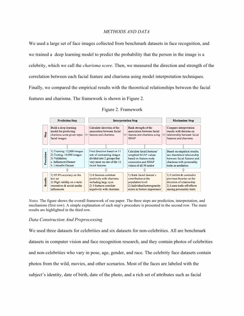
features and charisma. The framework is shown in Figure 2.

Figure 2. Framework

Notes. The figure shows the overall framework of our paper. The three steps are prediction, interpretation, and mechanism (first row). A simple explanation of each step’s procedure is presented in the second row. The main results are highlighted in the third row. Data Construction And Preprocessing

We used three datasets for celebrities and six datasets for non-celebrities. All are benchmark

datasets in computer vision and face recognition research, and they contain photos of celebrities

and non-celebrities who vary in pose, age, gender, and race. The celebrity face datasets contain

photos from the wild, movies, and other scenarios. Most of the faces are labeled with the

subject’s identity, date of birth, date of the photo, and a rich set of attributes such as facial

landmark locations, attractiveness, lip size, nose size, and hair color (Liu et al. 2015). The non-

celebrity face datasets contain photos from social media, a lab (Ma et al. 2015), and the internet.

Some face photos are labeled with attributes including facial expression, emotion, head pose,

hair color, facial landmarks, and accessories (Wang and Tang 2009).

In total, we had 22,000 images to divide between the training and testing sets. Of the

subjects in the 11,000 celebrity photos, 29.43% were female; 0.02% were below age 20, 82.28%

were age 20–40, and 17.63% were age 40–60; 9.14% were Asian, 7.27% were Black, 1.16%

were Indian, 9.36% were Latino/Hispanic, 8.01% were Middle Eastern, and 65.06% were White.

Of the subjects in the 11,000 non-celebrity photos, 28.62% were female; 0.33% were below age

20, 93.56% were age 20–40, and 6.11% were age 40–60; 17.74% were Asian, 5.98% were

Black, 1.32% were Indian, 11.55% were Latino/Hispanic, 7.09% were Middle Eastern, and

56.33% were White.4 In Web Appendix A, we provide detailed descriptions and statistics for

each of the nine datasets.

Data preprocessing. We preprocessed the images to address variations in size,

face/background ratio, direction, and illumination. First, we aligned and straightened the faces

(Kazemi and Sullivan 2014; Kovenko 2019) to reduce noise from variation in position and

direction.5 We cropped each face to standardize the face/background ratio and then resized the

images to 224X224X3 pixels, the required input size for the pre-trained ResNet-50 model.

Following previous literature, we normalized illumination (Zhang et al. 2007) to address

systematic differences between datasets (otherwise, the model might learn to differentiate

celebrity faces from non-celebrity faces based on the brightness of the image). We also rescaled

4 The age, gender, and race of each face image was detected using the Deepface framework based on VGG-Face in python (Serengil and Ozpinar 2020). 5 For preprocessing, we followed Kovenko (2019).

the pixels from 0 to 1 and augmented the data by flipping and tilting the images in the training

set (Jung et al. 2017) to mitigate the overfitting problem and enhance the model’s robustness.

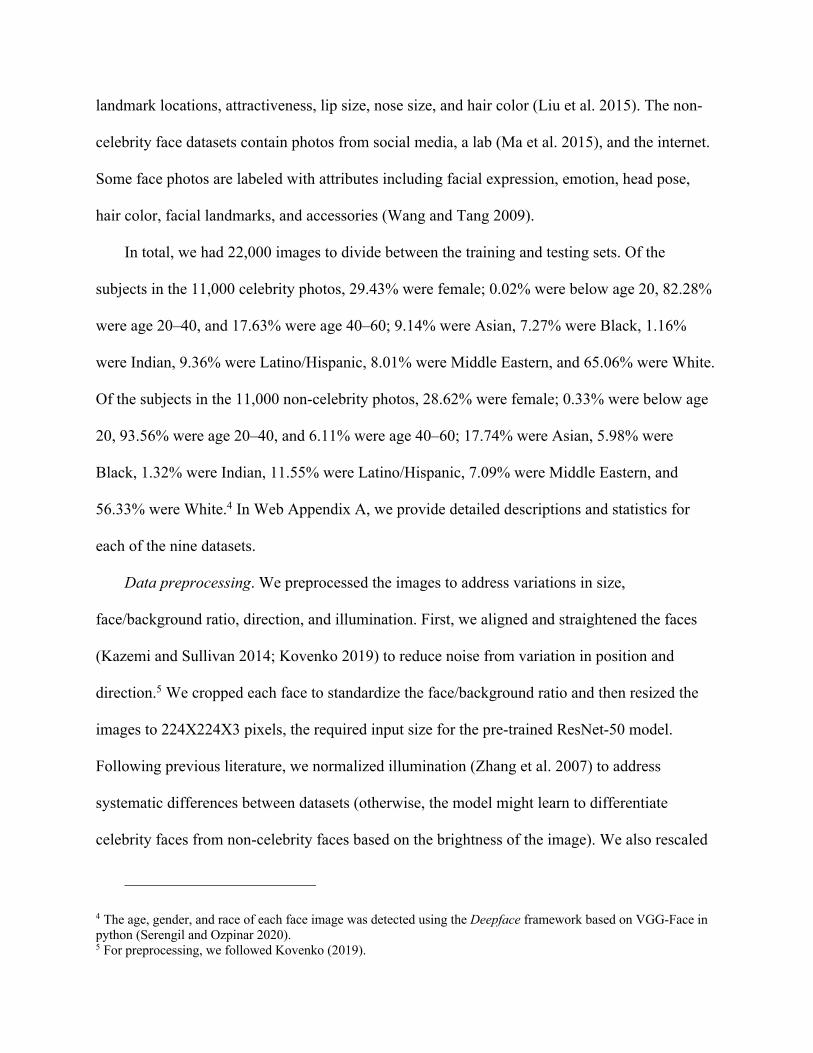
Figure 3 illustrates the preprocessing steps.

Figure 3. Face Image Preprocessing Steps

Notes. In preprocessing, we 1) detected the human face, nose, and eyes in the image, 2) rotated the image around the nose to straighten the face, 3) cropped the face from the image, 4) resized the image to 224×224×3 pixels, and 5) normalized illumination. Details of each preprocessing step and more examples are in Appendix B. Prediction Step

We used a supervised deep learning model that takes an image as input and outputs the

probability that the image is of a celebrity (i.e., our charisma score). For the backbone structure,

we employed ResNet-50 (He et al. 2016), a widely adopted computer vision deep learning

architecture that was pretrained on more than a million images from the ImageNet database. We

chose ResNet-50 for several advantageous features, including fast optimization and easy

accuracy gain with greatly increased depth. Since the backbone ResNet-50 was pretrained on a

task different from ours, we added a customized dense layer with 50 nodes and a sigmoid layer

for binary classification (celebrity or non-celebrity) on top of the ResNet-50 layer. The model

structure is shown in Figure 4, and Web Appendix B describes the model architecture and layers

in detail.

In addition to the pre-processing steps described in Section 3.1.1, we took several steps to

improve the model’s performance. First, we tested different variants of the ResNet-50 model and

selected the one with the highest out-of-sample prediction accuracy and a stable optimization

curve (lower variation in convergence). Second, we experimented with five optimizers: AdaGrad

(Dean et al. 2012), SGD (Bottou 1998), AdaDelta (Zeiler 2012), Adam (Kingma and Ba 2015),

and RMSprop. We achieved the highest accuracy and most stable optimization with the AdaGrad

optimizer (combined with preprocessing). Please see the Web Appendix B for details.

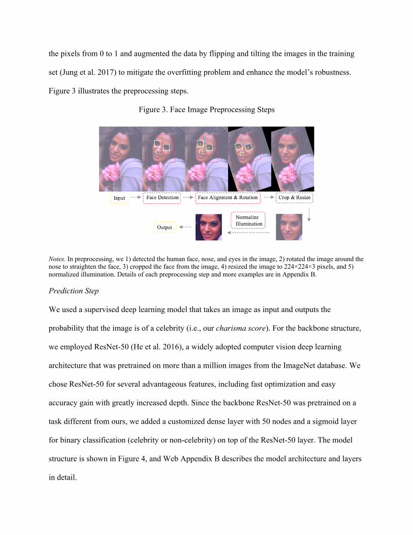
Figure 4. Architecture of the Classification Model Based on ResNet-50

Notes. The figure shows the structure of our classification model. The input was an image of 224×224×3 pixels. The backbone structure was ResNet-50; the colors denote the layer types (see Web Appendix B for details). We added a customized dense layer with 50 nodes before the final output, which was the probability that the subject in the image was a celebrity (i.e., our charisma score). The 3D Backbone (ResNet-50) was plotted using the model visualization python package -visualkeras. Interpretation Step

We interpreted the black-box deep learning model created in the prediction step by linking the 11

facial features discussed in Section 2.1 with the deep learning model. We produced two results:

the direction of the correlation between each facial feature and charisma and the contribution

ranking of the facial features to charisma.

Direction of the correlation between each facial feature and charisma. To test the

hypotheses in Section 2.1, we created a contrasting dataset for each facial feature. That is, we

selected and/or manipulated images to create two groups of images, labeled group 1 and group 2,

that varied dramatically in the focal feature, and we calculated the average charisma score of the

two groups of images using our deep learning model. For instance, for the facial width-to-height

ratio, we stretched the face in the image horizontally to create wider faces (group 1) and

vertically to create longer faces (group 2); the two groups had approximately the same facial

features except for the width-to-height ratio. A higher average charisma score in group 1 (group

2) would indicate that at the population level, wider (narrower) faces are associated with higher

(lower) charisma, implying a positive correlation between the width-to-height ratio and

charisma. We repeated this approach for all 11 facial features. The selection/manipulation

processes and examples of contrasting images are provided in Web Appendix C, Table W2.

Ranking the contributions of the facial features to charisma. The interpretation of black box

deep learning models is a recent frontier in the computer science and machine learning

communities. We elicited the relative importance of the facial features by ranking the 50 nodes

(described in Section 3.2) and then calculating the weighted contribution of each facial feature

based on the feature-node connections. In this way, we empirically established the relations

between the theoretical facial features and the nodes that captured their contributions. As long as

we knew the contribution of each node to the charisma score, we could deduce the contributions

of the facial features and explain why any given face is considered charismatic or not.

We zoomed into the 50-D layer of the deep learning model and the activation values of the

50 nodes mainly because the 50-D layer is where the features go into the final classification.

Therefore, these 50 nodes captured important variations in the facial features that finally

determined the charisma score. The activation value of a node represented how much the node

was activated by capturing certain features and could be viewed as a ranking of the node. If a

node captured a feature that was important in differentiating celebrity faces from non-celebrity

faces, the node was often activated. Using the set of images that had a large and obvious

variation on each given feature constructed as inputs (see Web Appendix C for details), we

calculated the activation value of each node on the 50-D layer. For instance, for the width-to-

height ratio feature, we compared wider faces (group 1) with longer faces (group 2) using the

Wasserstein distance.6 The node with the largest distance was then regarded as the node that

captured the width-to-height ratio feature. The above process was repeated for all theoretical

facial features stated in the literature review.

We applied XAI methods to calculate the contribution of each node to the charisma score.

We applied SHAP, a state-of-the-art XAI method (Lundberg and Lee 2017). SHAP is based on

cooperative game theory, which assumes that a finite set of players form the grand coalition, and

a characteristic function describes all possible payoffs that can be gained by forming different

coalitions. SHAP explains the output of any machine learning model and connects the optimal

credit allocation with local explanations using classic Shapley values (Shapley 1953) from game

theory and related extensions. Although several XAI methods exist, SHAP is the only one that

satisfies local accuracy, consistency, and missingness (see Web Appendix D for a discussion).

We assumed that the input node value from the second-to-last layer to the final sigmoid

layer was the set of players, and the final output (the probability that the inputted face was a

celebrity) was the payoff. We built a new XGBoost tree model (Chen and Guestrin 2016) and

implemented the Tree SHAP algorithm. We chose Tree SHAP over Deep SHAP because the

former is much faster in computation, computes the exact Shapley values instead of

6 The Wasserstein distance is a distance function defined between probability distributions. The detailed and accurate definition can be found in Petitjean (2002) and Arjovsky et al. (2017).

approximated values, and better visualizes the contribution of each input feature (Lundberg et al.

2020). For details, see Web Appendix D.

The input features of our tree model were the 50 node values from the second-to-last dense

layer, and the output values were the classification outcomes (celebrity versus non-celebrity). To

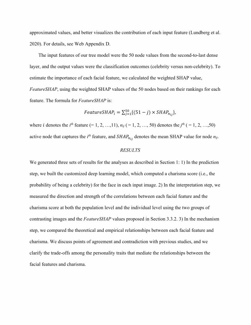
estimate the importance of each facial feature, we calculated the weighted SHAP value,

FeatureSHAP, using the weighted SHAP values of the 50 nodes based on their rankings for each

feature. The formula for FeatureSHAP is:

!"#$%&"'()*! = ∑ {(51 − 2) × '()*"!"}#$%&' ,

where 6 denotes the ith feature (= 1, 2, …,11), nij ( = 1, 2, …, 50) denotes the jth ( = 1, 2, …,50)

active node that captures the ith feature, and '()*"!" denotes the mean SHAP value for node nij.

RESULTS

We generated three sets of results for the analyses as described in Section 1: 1) In the prediction

step, we built the customized deep learning model, which computed a charisma score (i.e., the

probability of being a celebrity) for the face in each input image. 2) In the interpretation step, we

measured the direction and strength of the correlations between each facial feature and the

charisma score at both the population level and the individual level using the two groups of

contrasting images and the FeatureSHAP values proposed in Section 3.3.2. 3) In the mechanism

step, we compared the theoretical and empirical relationships between each facial feature and

charisma. We discuss points of agreement and contradiction with previous studies, and we

clarify the trade-offs among the personality traits that mediate the relationships between the

facial features and charisma.

Prediction Step

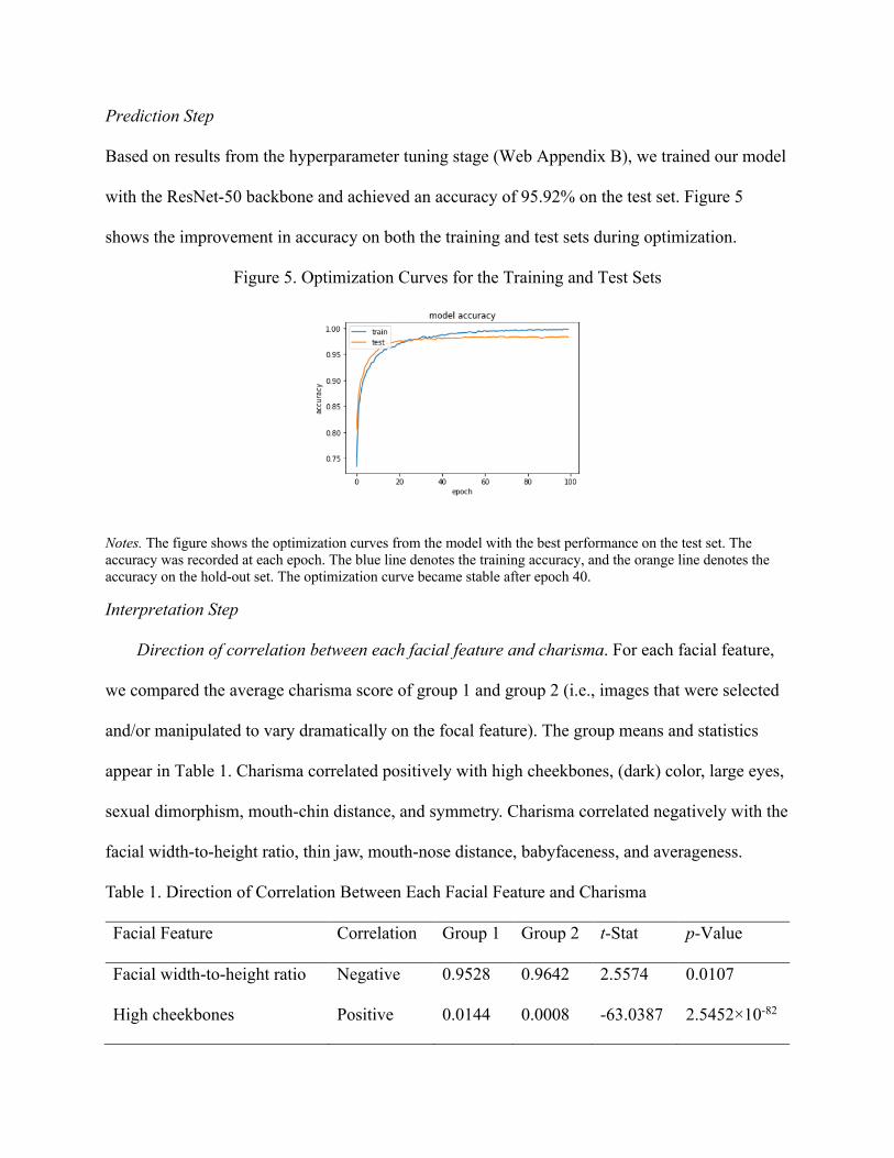
Based on results from the hyperparameter tuning stage (Web Appendix B), we trained our model

with the ResNet-50 backbone and achieved an accuracy of 95.92% on the test set. Figure 5

shows the improvement in accuracy on both the training and test sets during optimization.

Figure 5. Optimization Curves for the Training and Test Sets

Notes. The figure shows the optimization curves from the model with the best performance on the test set. The accuracy was recorded at each epoch. The blue line denotes the training accuracy, and the orange line denotes the accuracy on the hold-out set. The optimization curve became stable after epoch 40.

Interpretation Step

Direction of correlation between each facial feature and charisma. For each facial feature,

we compared the average charisma score of group 1 and group 2 (i.e., images that were selected

and/or manipulated to vary dramatically on the focal feature). The group means and statistics

appear in Table 1. Charisma correlated positively with high cheekbones, (dark) color, large eyes,

sexual dimorphism, mouth-chin distance, and symmetry. Charisma correlated negatively with the

facial width-to-height ratio, thin jaw, mouth-nose distance, babyfaceness, and averageness.

Table 1. Direction of Correlation Between Each Facial Feature and Charisma

Facial Feature Correlation Group 1 Group 2 t-Stat p-Value

Facial width-to-height ratio Negative 0.9528 0.9642 2.5574 0.0107

High cheekbones Positive 0.0144 0.0008 -63.0387 2.5452×10-82

(Dark) Color Positive 0.0057 0.0007 -36.8030 1.4554×10-59

Thin jaw Negative 0.0016 0.0085 1.5442 0.1257

Mouth-nose distance Negative 0.0019 0.0021 0.2403 0.8106

Large eyes Positive 0.0053 0.0031 -2.3870 0.0189

Sex dimorphism Positive 0.6331 0.2983 -19.1865 7.2912×10-62

Mouth-chin distance Positive 0.0024 0.0015 -1.5784 0.1176

Babyfaceness Negative 0.0013 0.0046 1.7880 0.0768

Symmetry Positive 0.0067 0.0013 -14.5719 2.2536×10-26

Averageness Negative 0.8972 0.9062 0.9594 0.3378

Notes. The table shows the direction of each facial feature’s correlation with charisma. The Group 1 and Group 2 columns provide the mean charisma score for the sets of selected/manipulated images explained in Table 1. The t-Stat column compares the charisma score distributions between Group 1 and Group 2 with a two-tailed test of the population mean with unknown variance. The p-Value column denotes the p-value for the corresponding t-statistics.

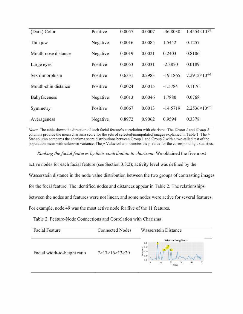
Ranking the facial features by their contribution to charisma. We obtained the five most

active nodes for each facial feature (see Section 3.3.2); activity level was defined by the

Wasserstein distance in the node value distribution between the two groups of contrasting images

for the focal feature. The identified nodes and distances appear in Table 2. The relationships

between the nodes and features were not linear, and some nodes were active for several features.

For example, node 49 was the most active node for five of the 11 features.

Table 2. Feature-Node Connections and Correlation with Charisma

Facial Feature Connected Nodes Wasserstein Distance

Facial width-to-height ratio 7>17>16>13>20

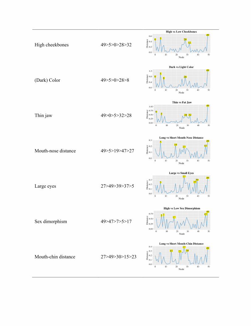
High cheekbones 49>5>0>28>32

(Dark) Color 49>5>0>28>8

Thin jaw 49>0>5>32>28

Mouth-nose distance 49>5>19>47>27

Large eyes 27>49>39>37>5

Sex dimorphism 49>47>7>5>17

Mouth-chin distance 27>49>30>15>23

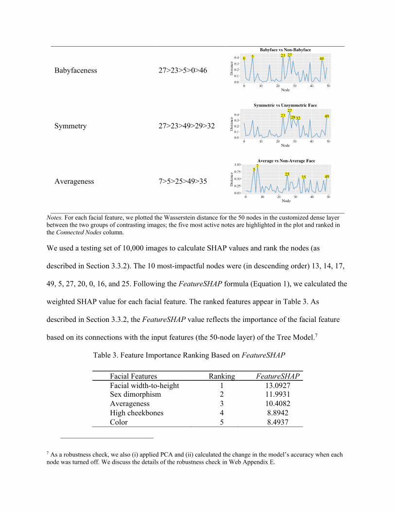
Babyfaceness 27>23>5>0>46

Symmetry 27>23>49>29>32

Averageness 7>5>25>49>35

Notes. For each facial feature, we plotted the Wasserstein distance for the 50 nodes in the customized dense layer between the two groups of contrasting images; the five most active notes are highlighted in the plot and ranked in the Connected Nodes column. We used a testing set of 10,000 images to calculate SHAP values and rank the nodes (as

described in Section 3.3.2). The 10 most-impactful nodes were (in descending order) 13, 14, 17,

49, 5, 27, 20, 0, 16, and 25. Following the FeatureSHAP formula (Equation 1), we calculated the

weighted SHAP value for each facial feature. The ranked features appear in Table 3. As

described in Section 3.3.2, the FeatureSHAP value reflects the importance of the facial feature

based on its connections with the input features (the 50-node layer) of the Tree Model.7

Table 3. Feature Importance Ranking Based on FeatureSHAP

Facial Features Ranking FeatureSHAP Facial width-to-height

ratio

1 13.0927 Sex dimorphism 2 11.9931 Averageness 3 10.4082 High cheekbones 4 8.8942 Color 5 8.4937

7 As a robustness check, we also (i) applied PCA and (ii) calculated the change in the model’s accuracy when each node was turned off. We discuss the details of the robustness check in Web Appendix E.

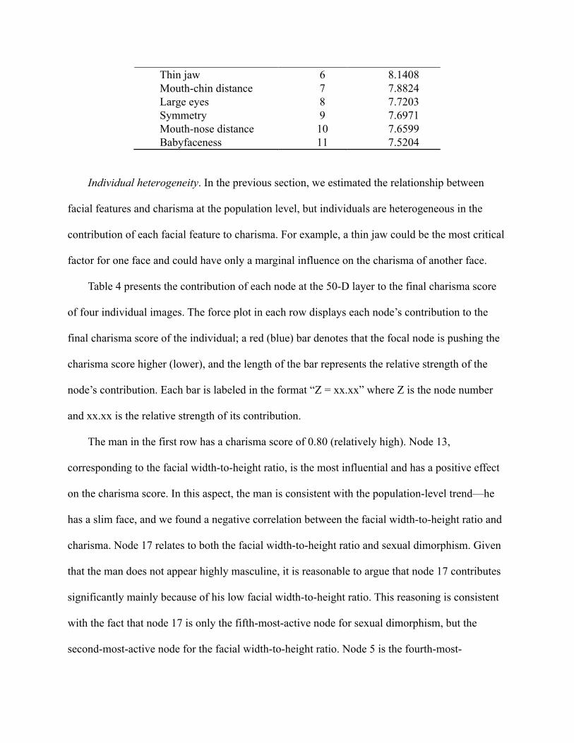
Thin jaw 6 8.1408 Mouth-chin distance 7 7.8824 Large eyes 8 7.7203 Symmetry 9 7.6971 Mouth-nose distance 10 7.6599 Babyfaceness 11 7.5204

Individual heterogeneity. In the previous section, we estimated the relationship between

facial features and charisma at the population level, but individuals are heterogeneous in the

contribution of each facial feature to charisma. For example, a thin jaw could be the most critical

factor for one face and could have only a marginal influence on the charisma of another face.

Table 4 presents the contribution of each node at the 50-D layer to the final charisma score

of four individual images. The force plot in each row displays each node’s contribution to the

final charisma score of the individual; a red (blue) bar denotes that the focal node is pushing the

charisma score higher (lower), and the length of the bar represents the relative strength of the

node’s contribution. Each bar is labeled in the format “Z = xx.xx” where Z is the node number

and xx.xx is the relative strength of its contribution.

The man in the first row has a charisma score of 0.80 (relatively high). Node 13,

corresponding to the facial width-to-height ratio, is the most influential and has a positive effect

on the charisma score. In this aspect, the man is consistent with the population-level trend—he

has a slim face, and we found a negative correlation between the facial width-to-height ratio and

charisma. Node 17 relates to both the facial width-to-height ratio and sexual dimorphism. Given

that the man does not appear highly masculine, it is reasonable to argue that node 17 contributes

significantly mainly because of his low facial width-to-height ratio. This reasoning is consistent

with the fact that node 17 is only the fifth-most-active node for sexual dimorphism, but the

second-most-active node for the facial width-to-height ratio. Node 5 is the fourth-most-

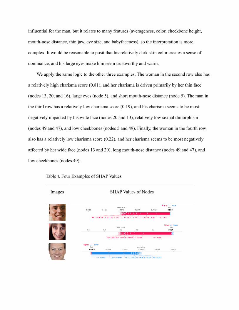
influential for the man, but it relates to many features (averageness, color, cheekbone height,

mouth-nose distance, thin jaw, eye size, and babyfaceness), so the interpretation is more

complex. It would be reasonable to posit that his relatively dark skin color creates a sense of

dominance, and his large eyes make him seem trustworthy and warm.

We apply the same logic to the other three examples. The woman in the second row also has

a relatively high charisma score (0.81), and her charisma is driven primarily by her thin face

(nodes 13, 20, and 16), large eyes (node 5), and short mouth-nose distance (node 5). The man in

the third row has a relatively low charisma score (0.19), and his charisma seems to be most

negatively impacted by his wide face (nodes 20 and 13), relatively low sexual dimorphism

(nodes 49 and 47), and low cheekbones (nodes 5 and 49). Finally, the woman in the fourth row

also has a relatively low charisma score (0.22), and her charisma seems to be most negatively

affected by her wide face (nodes 13 and 20), long mouth-nose distance (nodes 49 and 47), and

low cheekbones (nodes 49).

Table 4. Four Examples of SHAP Values

Images SHAP Values of Nodes

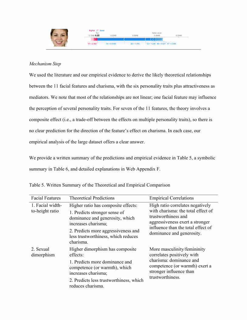
Mechanism Step

We used the literature and our empirical evidence to derive the likely theoretical relationships

between the 11 facial features and charisma, with the six personality traits plus attractiveness as

mediators. We note that most of the relationships are not linear; one facial feature may influence

the perception of several personality traits. For seven of the 11 features, the theory involves a

composite effect (i.e., a trade-off between the effects on multiple personality traits), so there is

no clear prediction for the direction of the feature’s effect on charisma. In each case, our

empirical analysis of the large dataset offers a clear answer.

We provide a written summary of the predictions and empirical evidence in Table 5, a symbolic

summary in Table 6, and detailed explanations in Web Appendix F.

Table 5. Written Summary of the Theoretical and Empirical Comparison

Facial Features Theoretical Predictions Empirical Correlations 1. Facial width-to-height ratio

Higher ratio has composite effects: 1. Predicts stronger sense of dominance and generosity, which increases charisma; 2. Predicts more aggressiveness and less trustworthiness, which reduces charisma.

High ratio correlates negatively with charisma: the total effect of trustworthiness and aggressiveness exert a stronger influence than the total effect of dominance and generosity.

2. Sexual dimorphism

Higher dimorphism has composite effects: 1. Predicts more dominance and competence (or warmth), which increases charisma; 2. Predicts less trustworthiness, which reduces charisma.

More masculinity/femininity correlates positively with charisma: dominance and competence (or warmth) exert a stronger influence than trustworthiness.

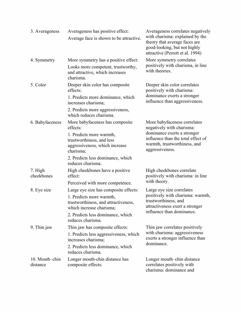
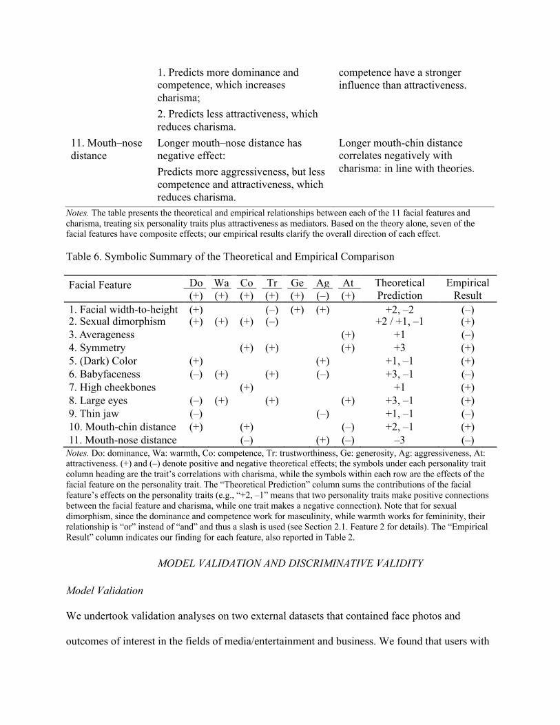
3. Averageness Averageness has positive effect: Average face is shown to be attractive.

Averageness correlates negatively with charisma: explained by the theory that average faces are good-looking, but not highly attractive (Perrett et al. 1994)

4. Symmetry More symmetry has a positive effect: Looks more competent, trustworthy, and attractive, which increases charisma.

More symmetry correlates positively with charisma, in line with theories.

5. Color Deeper skin color has composite effects: 1. Predicts more dominance, which increases charisma; 2. Predicts more aggressiveness, which reduces charisma.

Deeper skin color correlates positively with charisma: dominance exerts a stronger influence than aggressiveness.

6. Babyfaceness More babyfaceness has composite effects: 1. Predicts more warmth, trustworthiness, and less aggressiveness, which increase charisma; 2. Predicts less dominance, which reduces charisma.

More babyfaceness correlates negatively with charisma: dominance exerts a stronger influence than the total effect of warmth, trustworthiness, and aggressiveness.

7. High cheekbones

High cheekbones have a positive effect: Perceived with more competence.

High cheekbones correlate positively with charisma: in line with theory.

8. Eye size Large eye size has composite effects: 1. Predicts more warmth, trustworthiness, and attractiveness, which increase charisma; 2. Predicts less dominance, which reduces charisma.

Large eye size correlates positively with charisma: warmth, trustworthiness, and attractiveness exert a stronger influence than dominance.

9. Thin jaw Thin jaw has composite effects: 1. Predicts less aggressiveness, which increases charisma; 2. Predicts less dominance, which reduces charisma.

Thin jaw correlates positively with charisma: aggressiveness exerts a stronger influence than dominance.

10. Mouth–chin distance

Longer mouth-chin distance has composite effects:

Longer mouth–chin distance correlates positively with charisma: dominance and

1. Predicts more dominance and competence, which increases charisma; 2. Predicts less attractiveness, which reduces charisma.

competence have a stronger influence than attractiveness.

11. Mouth–nose distance

Longer mouth–nose distance has negative effect: Predicts more aggressiveness, but less competence and attractiveness, which reduces charisma.

Longer mouth-chin distance correlates negatively with charisma: in line with theories.

Notes. The table presents the theoretical and empirical relationships between each of the 11 facial features and charisma, treating six personality traits plus attractiveness as mediators. Based on the theory alone, seven of the facial features have composite effects; our empirical results clarify the overall direction of each effect.

Table 6. Symbolic Summary of the Theoretical and Empirical Comparison

Facial Feature Do

(+)

Wa

(+)

Co

(+)

Tr

(+)

Ge

(+)

Ag

(-)

At

(0)

Theoretical Prediction

Empirical Result (+) (+) (+) (+) (+) (–) (+)

1. Facial width-to-height Ratio

(+) (–) (+) (+) +2, –2 (–) 2. Sexual dimorphism (+) (+) (+) (–) +2 / +1, –1 (+) 3. Averageness (+) +1 (–) 4. Symmetry (+) (+) (+) +3 (+) 5. (Dark) Color (+) (+) +1, –1 (+) 6. Babyfaceness (–) (+) (+) (–) +3, –1 (–) 7. High cheekbones (+) +1 (+) 8. Large eyes (–) (+) (+) (+) +3, –1 (+) 9. Thin jaw (–) (–) +1, –1 (–) 10. Mouth-chin distance (+) (+) (–) +2, –1 (+) 11. Mouth-nose distance (–) (+) (–) –3 (–)

Notes. Do: dominance, Wa: warmth, Co: competence, Tr: trustworthiness, Ge: generosity, Ag: aggressiveness, At: attractiveness. (+) and (–) denote positive and negative theoretical effects; the symbols under each personality trait column heading are the trait’s correlations with charisma, while the symbols within each row are the effects of the facial feature on the personality trait. The “Theoretical Prediction” column sums the contributions of the facial feature’s effects on the personality traits (e.g., “+2, –1” means that two personality traits make positive connections between the facial feature and charisma, while one trait makes a negative connection). Note that for sexual dimorphism, since the dominance and competence work for masculinity, while warmth works for femininity, their relationship is “or” instead of “and” and thus a slash is used (see Section 2.1. Feature 2 for details). The “Empirical Result” column indicates our finding for each feature, also reported in Table 2.

MODEL VALIDATION AND DISCRIMINATIVE VALIDITY

Model Validation

We undertook validation analyses on two external datasets that contained face photos and

outcomes of interest in the fields of media/entertainment and business. We found that users with

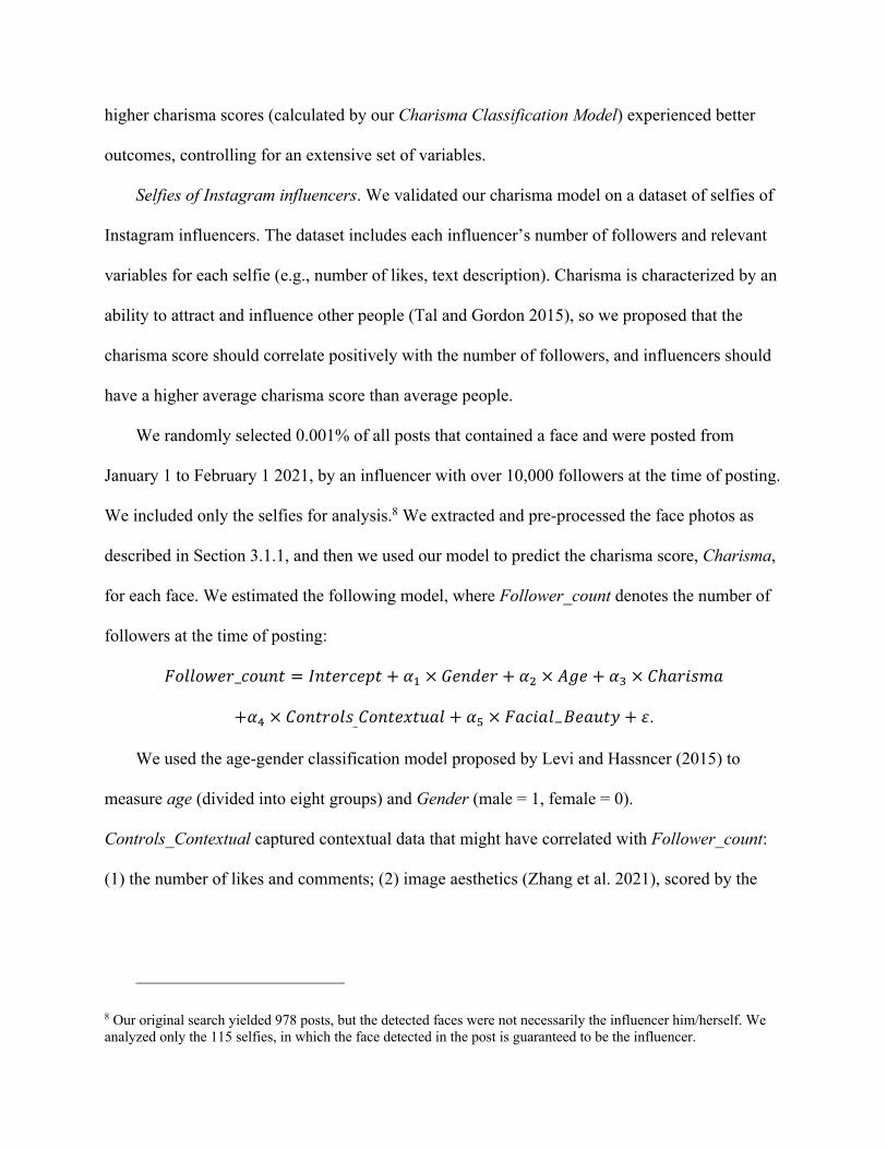
higher charisma scores (calculated by our Charisma Classification Model) experienced better

outcomes, controlling for an extensive set of variables.

Selfies of Instagram influencers. We validated our charisma model on a dataset of selfies of

Instagram influencers. The dataset includes each influencer’s number of followers and relevant

variables for each selfie (e.g., number of likes, text description). Charisma is characterized by an

ability to attract and influence other people (Tal and Gordon 2015), so we proposed that the

charisma score should correlate positively with the number of followers, and influencers should

have a higher average charisma score than average people.

We randomly selected 0.001% of all posts that contained a face and were posted from

January 1 to February 1 2021, by an influencer with over 10,000 followers at the time of posting.

We included only the selfies for analysis.8 We extracted and pre-processed the face photos as

described in Section 3.1.1, and then we used our model to predict the charisma score, Charisma,

for each face. We estimated the following model, where Follower_count denotes the number of

followers at the time of posting:

!78879"&_;7%<$ = =<$"&;">$ + @' × A"<B"& + @( × )C" + @) × Dℎ#&6FG#

+@* × D7<$&78F_D7<$"H$%#8 + @# × !#;6#8,I"#%$J + K.

We used the age-gender classification model proposed by Levi and Hassncer (2015) to

measure age (divided into eight groups) and Gender (male = 1, female = 0).

Controls_Contextual captured contextual data that might have correlated with Follower_count:

(1) the number of likes and comments; (2) image aesthetics (Zhang et al. 2021), scored by the

8 Our original search yielded 978 posts, but the detected faces were not necessarily the influencer him/herself. We analyzed only the 115 selfies, in which the face detected in the post is guaranteed to be the influencer.

Neural Image Assessment framework proposed by Talebi and Milanfar (2018);9 (3) the text

description’s length, readability (Flesch 1948), and richness (Chotlos 1944); and (4) the text’s

sentiment, predicted using the VADER Sentiment Intensity Analyzer (Hutto and Gilbert 2014).

We included !#;6#8_I"#%$J, measured by the state-of-the-art ResNet-50 framework trained on

the SCUT-FBP5500 dataset (Liang et al. 2018), to tease out the impact of attractiveness from the

impact of charisma on the number of followers. The estimations results are in Web Appendix G.

In the estimation results of the full regression model and the models after feature selection

through Step AIC (Hock 1976), the charisma score had a positive and significant coefficient

across model specifications. Critically, influencers with higher charisma scores consistently had

more followers than influencers with lower charisma scores, even when including Facial Beauty

and Controls_Contextual. It is worth noting that physical attractiveness seemed to play only a

minor role in the number of followers: the estimated coefficient of Facial Beauty was

insignificant, the estimated coefficient of the charisma score essentially did not change with the

inclusion of Facial Beauty, and the multiple R2 barely changed when we excluded

Facial_Beauty from the model.

However, our results may be affected by selection bias—people who choose to become

influencers generally are more charismatic than the average population. To verify, we randomly

selected and analyzed another 115 selfies from one of the non-celebrity datasets, the Selfie

Dataset (not contained within the training set) and calculated the average charisma score. These

115 randomly-selected individuals had an average charisma score of only 0.2038, while the 115

influencers averaged 0.7304, confirming the selection bias.

9 The model has state-of-the-art performance at predicting the distribution of human opinions on image quality, trained on the AVA (Murray et al. 2012), TID2013 (Ponomarenko et al. 2013), and LIVE (Ghadiyaram and Bovik 2016) datasets.

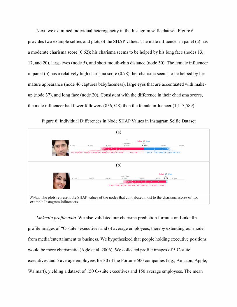
Next, we examined individual heterogeneity in the Instagram selfie dataset. Figure 6

provides two example selfies and plots of the SHAP values. The male influencer in panel (a) has

a moderate charisma score (0.62); his charisma seems to be helped by his long face (nodes 13,

17, and 20), large eyes (node 5), and short mouth-chin distance (node 30). The female influencer

in panel (b) has a relatively high charisma score (0.78); her charisma seems to be helped by her

mature appearance (node 46 captures babyfaceness), large eyes that are accentuated with make-

up (node 37), and long face (node 20). Consistent with the difference in their charisma scores,

the male influencer had fewer followers (856,548) than the female influencer (1,113,589).

Figure 6. Individual Differences in Node SHAP Values in Instagram Selfie Dataset

(a)

(b)

Notes. The plots represent the SHAP values of the nodes that contributed most to the charisma scores of two example Instagram influencers.

LinkedIn profile data. We also validated our charisma prediction formula on LinkedIn

profile images of “C-suite” executives and of average employees, thereby extending our model

from media/entertainment to business. We hypothesized that people holding executive positions

would be more charismatic (Agle et al. 2006). We collected profile images of 5 C-suite

executives and 5 average employees for 30 of the Fortune 500 companies (e.g., Amazon, Apple,

Walmart), yielding a dataset of 150 C-suite executives and 150 average employees. The mean

charisma score of the C-suite executives (0.8453) was significantly higher than the mean

charisma score of the average employees (0.1971, p-value = 1.0994×10-53 in lower-tail test of

population mean), demonstrating that our model translates well to the business context.

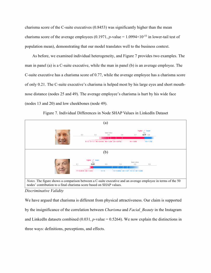
As before, we examined individual heterogeneity, and Figure 7 provides two examples. The

man in panel (a) is a C-suite executive, while the man in panel (b) is an average employee. The

C-suite executive has a charisma score of 0.77, while the average employee has a charisma score

of only 0.21. The C-suite executive’s charisma is helped most by his large eyes and short mouth-

nose distance (nodes 25 and 49). The average employee’s charisma is hurt by his wide face

(nodes 13 and 20) and low cheekbones (node 49).

Figure 7. Individual Differences in Node SHAP Values in LinkedIn Dataset

(a)

(b)

Notes. The figure shows a comparison between a C-suite executive and an average employee in terms of the 50 nodes’ contribution to a final charisma score based on SHAP values.

Discriminative Validity

We have argued that charisma is different from physical attractiveness. Our claim is supported

by the insignificance of the correlation between Charisma and Facial_Beauty in the Instagram

and LinkedIn datasets combined (0.031, p-value = 0.5264). We now explain the distinctions in

three ways: definitions, perceptions, and effects.

First, the definitions of charisma and attractiveness emphasize different qualities. Weber’s

definition of charisma focuses on the perception that the person is endowed with exceptional

powers and qualities that elicit devotion from others (Weber 1947). Meanwhile, attractiveness

centers around physical appearance, including facial features and body proportions (Dion,

Berscheid, and Walster 1972). Thus, while charisma stresses internal qualities such as power and

leadership, attractiveness is defined by one’s external appearance.

Second, people develop perceptions of charisma and attractiveness in different ways.

Attractiveness is perceived through a person’s static appearance, while charisma is perceived

through both physical appearance and dynamic nonverbal cues that convey emotions (Ekman,

Friesen, and Ellsworth 1972). Charisma may be best understood as a combination of the desire

and ability to communicate emotions and inspire others, so socioemotional interactions are at

least as important as physical appearance (Friedman 1980).

Third, charisma and attractiveness have different effects on the depth and duration of

perception. People tend to describe attractive friends as simply good-looking, while charismatic

friends receive a variety of descriptions—they are colorful, entertaining, popular, and the center

of social interactions (Friedman 1988). In other words, while attractiveness gives rise to

unidimensional impressions, charisma creates a multi-faceted character in perceivers’ minds,

influencing their emotions and attracting their attention from deep inside. Also, while people

initially may come together because of physical appearance (Swami and Furnham 2008),

charisma is more important for creating long-lasting relationships (Chase 2016).

Mitigation of Racial Bias in Marketing

One valid concern about the application of our charisma scoring model is the potential for racial

bias. To test for the presence of bias, we estimated the charisma scores of 150 Black people and

150 white people selected randomly from the CFD. Indeed, the average charisma score of the

white people was 66.2181% higher than that of the Black people (p-value = 0.0654). We propose

gray-scale images as a potential solution. When we re-estimated the charisma scores of the same

300 people using gray-scale images, the advantage of white people became insignificant

(39.6195%; p-value = 0.1023).

GENERAL DISCUSSION AND CONCLUSIONS

Our research represents the first empirical attempt to characterize the relationships between

charisma and facial features. We built a deep learning model that predicts someone’s charisma

score based on a photo of their face. The model achieved high accuracy on the hold-out test

sample and was validated in the contexts of media/entertainment (using selfies of Instagram

influencers and average individuals) and business (using LinkedIn profile pictures of C-suite

executives and average employees). Our use of facial analytics on a large dataset enabled us to

interpret the direction and strength of the correlation between each of the 11 facial features and

charisma and to derive a charisma formula (Equation 1) that uses SHAP to rank the features by

the size of their contribution to charisma.

Theoretically, our research is among the first to comprehensively consolidate prior theories

on the correlations between facial features and charisma with personality traits as mediators. We

empirically verified that the correlations are complicated and nonlinear. The outcomes of the

trade-offs between personality traits depend on the situation. Past literature has suggested

diverging (or contradictory) relations between charisma and facial features. Our results support

some of these relations (e.g., charisma is hurt by a higher facial width-to-height ratio and thinner

jaw) and contradict others (e.g., the correlation between averageness and charisma is

theoretically positive but empirically negative). While previous research on facial feature

analysis has used regressions and experiments or built multidimensional face space, our study

creatively and methodologically developed a nonparametric deep learning model with high

accuracy that can be scaled to large and unstructured data.

Two of our core metrics—the Charisma Score and FeatureSHAP—are easily scaled and

may be useful for both companies and individuals. The Charisma Score could aid decision-

making regarding the investment in individuals or images when charisma is key to success. In

advertising, human photos need to look highly charismatic to influence consumers’ purchase

intentions (Xiao and Ding 2014), so content engineering companies could benefit from using

charisma scores to find the optimal images. A company that wishes to cooperate with social

media influencers might benefit from using the charisma score as a selection criterion, as the

ability to emotionally influence the audience and followers is critical (Friedman et al. 1980;

Keating 2002). The charisma score might also be useful for individuals who are seeking

guidance on whether they are well suited for a career as an actor, influencer, politician,

executive, or another role that requires the ability to exert an emotional influence on one’s

audience. When choosing leaders for other managerial positions, the recruiters can refer to our

algorithm to recruit the candidates with the highest charisma scores as one of the metrics if

there’s limited time for interview.

Meanwhile, FeatureSHAP could be used to hone an individual’s appearance in real time.

For example, perhaps a start-up founder is recording a pitch video to persuade prospective

investors.10 The founder could record a test clip, run our model on a series of images from the

test clip, and identify the contribution of each facial feature to the charisma score. Then, the

10 Startups that are applying for accelerator programs are required to submit a self-introductory pitch video. The accelerators make funding decisions based on the pitch video along with other materials. See Hu and Ma (2020) for more details.

founder could optimize their charisma by manipulating certain facial features (e.g., cosmetics

and camera angles can manipulate one’s perceived jaw width, skin color, and cheekbone height).

For talent agency companies, FeatureSHAP values could similarly inform adjustments to a

celebrity’s make-up, hair style, or other flexible elements of appearance (Sarwer et al. 1998).

Based on FeatureSHAP, candidates in political elections can also make themselves appear to be

more charismatic for public speaking engagements via the adjustment of makeup and hairstyle.

This study has a few limitations that suggest areas for future research. First, a few of the facial

features had a surprising empirical relationship with charisma. The most notable example is

averageness, which theoretically should increase attractiveness and thereby is likely to increase

charisma—but we found a negative correlation. This suggests that other relationships between

facial features and perceived personality traits are worth exploring. Second, several facial

features have theoretical correlations with more than one personality trait and subsequently exert

composite effects (i.e., with both positive and negative components) on charisma. Although our

empirical results clarified the overall effect (e.g., the negative influence of babyfaceness due to

reduced dominance outweighs the positive influence due to increased warmth and

trustworthiness), the exact nature of the trade-offs between the personality traits remains unclear.

Future research investigating trade-off mechanisms may deepen our understanding of the

Charisma Score and FeatureSHAP metrics. Third, charisma may not apply equally to all

contexts. For instance, when recruiting candidates for engineering or technological positions,

charisma is relatively unimportant as people in such positions typically work alone or in small

teams and do not interface with the public on behalf of the company, so they have little need to

influence other people.

REFERENCES

Agle, Bradley R, Nandu J Nagarajan, Jeffrey A Sonnenfeld, and Dhinu Srinivasan (2006), “Does

CEO Charisma Matter? An Empirical Analysis of the Relationships among Organizational

Performance, Environmental Uncertainty, and Top Management Team Perceptions of CEO

Charisma,” The Academy of Management Journal, 49 (1), 161–74.

Alexander, Jeffrey C (2010), “The Celebrity-Icon,” Cultural Sociology, 4 (3), 323–36.

Alexander, Todorov, Mandisodza Anesu N, Goren Amir, and Hall Crystal C (2005), “Inferences

of Competence from Faces Predict Election Outcomes,” Science, 308 (5728), 1623–26.

Alley, Thomas R and Michael R Cunningham (1991), “Averaged Faces Are Attractive, but Very

Attractive Faces Are Not Average,” Psychological Science, 2 (2), 123–25.

Antonakis, John, Nicolas Bastardoz, Philippe Jacquart, and Boas Shamir (2016), “Charisma: An

Ill-Defined and Ill-Measured Gift,” Annual Review of Organizational Psychology and

Organizational Behavior, 3 (1), 293–319.

Arjovsky, Martin, Soumith Chintala, and Léon Bottou (2017), “Wasserstein Generative

Adversarial Networks,” in Proceedings of the 34th International Conference on Machine

Learning, Proceedings of Machine Learning Research, D. Precup and Y. W. Teh, eds.,

PMLR, 214–23.

Arthur, Michael B, Svetlana N Khapova, and Celeste P M Wilderom (2005), “Career success in

a boundaryless career world.,” Journal of Organizational Behavior, 26 (2), 177–202.

Avolio, Bruce J and Bernard M Bass (1988), “Transformational leadership, charisma, and

beyond.,” in Emerging leadership vistas., International leadership symposia series.,

Lexington, MA, England: Lexington Books/D. C. Heath and Com, 29–49.

Bass, Bernard M. (1985), Leadership and Performance beyond Expectations, Free Press.

Beck, Ulrich (2012), “Redefining the Sociological Project: The Cosmopolitan Challenge,”

Sociology, 46 (1), 7–12.

Berenson, Edward and Eva Giloi (2010), Celebrity, Fame, and Power in Nineteenth-Century

Europe, (E. BERENSON and E. V. A. GILOI, eds.), Berghahn Books.

Berscheid, Ellen and Elaine Hatfield (1978), Interpersonal attraction, Reading, Mass. : Addison-

Wesley Pub. Co., ©1978.

Bottou, Léon (1998), “Online Learning and Stochastic Approximations.”

Buss, Arnold H. and Mark Perry (1992), “The Aggression Questionnaire,” Journal of

Personality and Social Psychology, 63 (3), 452–59.

Carré, Justin M, Cheryl M McCormick, and Catherine J Mondloch (2009), “Facial Structure Is a

Reliable Cue of Aggressive Behavior,” Psychological Science, 20 (10), 1194–98.

Cattell, Raymond B (1950), Personality: A systematic theoretical and factual study, 1st ed.,

Personality: A systematic theoretical and factual study, 1st ed., New York, NY, US:

McGraw-Hill.

Chase, Alexander (2016), Unleash Your Charisma to Improve Your Social Skills and Create

Long Lasting Relationships with Everyone You Meet, CreateSpace Independent Publishing

Platform.

Chen, Tianqi and Carlos Guestrin (2016), “XGBoost: A Scalable Tree Boosting System,” in

Proceedings of the 22nd ACM SIGKDD International Conference on Knowledge Discovery

and Data Mining, KDD ’16, New York, NY, USA: Association for Computing Machinery,

785–94.

Chotlos, John W (1944), “IV. A statistical and comparative analysis of individual written

language samples.,” Psychological Monographs, 56 (2), 75–111.

Choudhury, Prithwiraj, Dan Wang, Natalie A Carlson, and Tarun Khanna (2019), “Machine

learning approaches to facial and text analysis: Discovering CEO oral communication

styles,” Strategic Management Journal, 40 (11), 1705–32.

Conger, Jay A, Rabindra N Kanungo, and Sanjay T Menon (2000), “Charismatic Leadership and

Follower Effects,” Journal of Organizational Behavior, 21 (7), 747–67.

Costa, Paul, R R McCrae, and T M Dembroski (1989), “Agreeableness versus antagonism:

Explication of a potential risk factor for CHD,” In Search of Coronary-prone Behavior:

Beyond Type A, 41–63.

Cunningham, M (1986), “Measuring the physical in physical attractiveness: quasi-experiments

on the sociobiology of female facial beauty,” Journal of Personality and Social Psychology,

50, 925–35.

Cunningham, M, A Barbee, and C L Pike (1990), “What do women want? Facialmetric

assessment of multiple motives in the perception of male facial physical attractiveness.,”

Journal of personality and social psychology, 59 1, 61–72.

Dean, Jeffrey, Greg Corrado, Rajat Monga, Kai Chen, Matthieu Devin, Mark Mao, Marc aurelio

Ranzato, Andrew Senior, Paul Tucker, Ke Yang, Quoc Le, and Andrew Ng (2012), “Large

Scale Distributed Deep Networks,” in Advances in Neural Information Processing Systems,

F. Pereira, C. J. C. Burges, L. Bottou, and K. Q. Weinberger, eds., Curran Associates, Inc.

Dion, Karen, Ellen Berscheid, and Elaine Walster (1972), “What is beautiful is good.,” Journal

of Personality and Social Psychology, 24 (3).

Dunn, Billie Schwab (2018), “What does your face say about you? Expert reveals the personality

traits of four celebrities based on their looks - and the secrets to ‘reading’ the people in your

life,” DailyMail.com.

Dvir, Taly, Dov Eden, Bruce J Avolio, and Boas Shamir (2002), “Impact of Transformational

Leadership on Follower Development and Performance: A Field Experiment,” The Academy

of Management Journal, 45 (4), 735–44.

Eberhardt, Jennifer L, Paul G Davies, Valerie J Purdie-Vaughns, and Sheri Lynn Johnson (2006),

“Looking Deathworthy: Perceived Stereotypicality of Black Defendants Predicts Capital-

Sentencing Outcomes,” Psychological Science, 17 (5), 383–86.

Eder, Donna (1985), “The Cycle of Popularity: Interpersonal Relations Among Female

Adolescents,” Sociology of Education, 58 (3), 154–65.

EKMAN, PAUL, WALLACE v FRIESEN, and PHOEBE ELLSWORTH (1972), “CHAPTER

XVII - Are Components of Facial Behavior Related to Observers’ Judgments of Emotion?,”

in Emotion in the Human Face, P. EKMAN, W. v FRIESEN, and P. ELLSWORTH, eds.,

Pergamon, 121–33.

Fink, Bernhard, Nick Neave, John T. Manning, and Karl Grammer (2005), “Facial symmetry and

the ‘big-five’ personality factors,” Personality and Individual Differences, 39 (3), 523–29.

Fink, Bernhard, Nick Neave, John T. Manning, and Karl Grammer (2006), “Facial symmetry and

judgements of attractiveness, health and personality,” Personality and Individual

Differences, 41 (3), 491–99.

FLESCH, R (1948), “A new readability yardstick.,” The Journal of applied psychology, 32 (3).

Friedman, H, L Prince, R Riggio, and M Dimatteo (1980), “Understanding and Assessing

Nonverbal Expressiveness: The Affective Communication Test.,” Journal of Personality

and Social Psychology, 39, 333–51.

Friedman, Howard S, Ronald E Riggio, and Daniel F Casella (1988), “Nonverbal Skill, Personal

Charisma, and Initial Attraction,” Personality and Social Psychology Bulletin, 14 (1), 203–

11.

Gangestad, S, J Simpson, A J Cousins, C Garver-Apgar, and P Christensen (2004), “Women’s

Preferences for Male Behavioral Displays Change Across the Menstrual Cycle,”

Psychological Science, 15, 203–7.

Gao, Huachao, Vikas Mittal, and Yinlong Zhang (2020), “The Differential Effect of Local–

Global Identity Among Males and Females: The Case of Price Sensitivity,” Journal of

Marketing Research, 57 (1), 173–91.

Ghadiyaram, D and A C Bovik (2016), “Massive Online Crowdsourced Study of Subjective and

Objective Picture Quality,” IEEE Transactions on Image Processing, 25 (1), 372–87.

Goffman, Erving (1959), “The Moral Career of the Mental Patient,” Psychiatry, 22 (2), 123–42.

Gorn, Gerald J, Yuwei Jiang, and Gita Venkataramani Johar (2008), “Babyfaces, Trait

Inferences, and Company Evaluations in a Public Relations Crisis,” Journal of Consumer

Research, 35 (1), 36–49.

Gray, Kurt, Adrian F Ward, and M Norton (2014), “Paying it forward: generalized reciprocity

and the limits of generosity.,” Journal of experimental psychology. General, 143 1, 247–54.

Griffin, Angela M and Judith H Langlois (2006), “Stereotype Directionality and Attractiveness

Stereotyping: Is Beauty Good or is Ugly Bad?,” Social cognition, 24 (2), 187–206.

Hartmann, Jochen, Mark Heitmann, Christina Schamp, and Oded Netzer (2021), “The Power of

Brand Selfies,” SSRN Electronic Journal.

He, K, X Zhang, S Ren, and J Sun (2016), “Deep Residual Learning for Image Recognition,” in

2016 IEEE Conference on Computer Vision and Pattern Recognition (CVPR), 770–78.

Hocking, R R (1976), “A Biometrics Invited Paper. The Analysis and Selection of Variables in

Linear Regression,” Biometrics, 32 (1), 1–49.

HOEGG, JOANDREA and MICHAEL v LEWIS (2011), “The Impact of Candidate Appearance

and Advertising Strategies on Election Results,” Journal of Marketing Research, 48 (5),

895–909.

House, Robert J. and Jane M. Howell (1992), “Personality and charismatic leadership,” The

Leadership Quarterly, 3 (2), 81–108.

House, Robert J, William D Spangler, and James Woycke (1991), “Personality and Charisma in

the U.S. Presidency: A Psychological Theory of Leader Effectiveness,” Administrative

Science Quarterly, 36 (3), 364–96.

Hu, Allen and Song Ma (2021), “Persuading Investors: A Video-Based Study,” Cambridge, MA.

Hutto, C and Eric Gilbert (2014), “VADER: A Parsimonious Rule-Based Model for Sentiment

Analysis of Social Media Text,” Proceedings of the International AAAI Conference on Web

and Social Media, 8 (1), 216–25.

“Infer the character of person from facial features” (2018), Onmanorama.

Joosse, Paul (2014), “Becoming a God: Max Weber and the social construction of charisma,”

Journal of Classical Sociology, 14 (3), 266–83.

Jung, Jaemin, Haeyeop Song, Youngju Kim, Hyunsuk Im, and Sewook Oh (2017), “Intrusion of

Software Robots into Journalism,” Comput. Hum. Behav., 71 (C), 291–98.

Kachur, Alexander, Evgeny Osin, Denis Davydov, Konstantin Shutilov, and Alexey

Novokshonov (2020), “Assessing the Big Five personality traits using real-life static facial

images,” Scientific Reports, 10 (1), 8487.

Kanter, Rosabeth Moss (2012), “Why You Need Charisma,” Harvard Business Review.

Kazemi, Vahid and Josephine Sullivan (2014), “One millisecond face alignment with an

ensemble of regression trees,” in 2014 IEEE Conference on Computer Vision and Pattern

Recognition, 1867–74.

Keating, C (1985), “Gender and the physiognomy of dominance and attractiveness.,” Social

Psychology Quarterly, 48, 61–70.

Keating, Caroline (2011), “Channelling Charisma through Face and Body Status Cues.”

Keating, Caroline F (2002), “Charismatic faces: Social status cues put face appeal in context.,” in

Facial attractiveness: Evolutionary, cognitive, and social perspectives., Advances in visual

cognition, vol. 1., Westport, CT, US: Ablex Publishing, 153–92.

Keating, Caroline F., Allan Mazur, and Marshall H. Segall (1981), “A cross-cultural exploration

of physiognomic traits of dominance and happiness,” Ethology and Sociobiology, 2 (1), 41–

48.

King, Patrick (2015), Everyday Charisma: Techniques for Mass Appeal, Charm, and Becoming a

Social Powerhouse, Createspace Independent Publishing Platform.

Kingma, Diederik P and Jimmy Ba (2015), “Adam: A Method for Stochastic Optimization,”

CoRR, abs/1412.6980.

Kovenko, Volodymyr (2019), “How to precisely align face in Python with OpenCv and Dlib,”

Medium.

Langlois, Judith H and Lori A Roggman (1990), “Attractive Faces Are Only Average,”

Psychological Science, 1 (2), 115–21.

Levi, G and T Hassncer (2015), “Age and gender classification using convolutional neural

networks,” in 2015 IEEE Conference on Computer Vision and Pattern Recognition

Workshops (CVPRW), 34–42.

Li, Yiyi and Ying Xie (2019), “Is a Picture Worth a Thousand Words? An Empirical Study of

Image Content and Social Media Engagement,” Journal of Marketing Research, 57 (1), 1–

19.

Liang, Lingyu, Luojun Lin, Lianwen Jin, Duorui Xie, and M Li (2018), “SCUT-FBP5500: A

Diverse Benchmark Dataset for Multi-Paradigm Facial Beauty Prediction,” 2018 24th

International Conference on Pattern Recognition (ICPR), 1598–1603.

Little, A C, B Jones, D Feinberg, and D Perrett (2014), “Men’s strategic preferences for

femininity in female faces.,” British journal of psychology, 105 3, 364–81.

Liu, Ziwei, Ping Luo, Xiaogang Wang, and Xiaoou Tang (2015), “Deep Learning Face

Attributes in the Wild,” 2015 IEEE International Conference on Computer Vision (ICCV),

3730–38.

Livingston, Robert W and Nicholas A Pearce (2009), “The Teddy-Bear Effect: Does Having a

Baby Face Benefit Black Chief Executive Officers?,” Psychological Science, 20 (10), 1229–

36.

Lundberg, Scott M, Gabriel Erion, Hugh Chen, Alex DeGrave, Jordan M Prutkin, Bala Nair,

Ronit Katz, Jonathan Himmelfarb, Nisha Bansal, and Su-In Lee (2020), “From local

explanations to global understanding with explainable AI for trees,” Nature Machine

Intelligence, 2 (1), 56–67.

Lundberg, Scott M and Su-In Lee (2017), “A Unified Approach to Interpreting Model

Predictions,” in Proceedings of the 31st International Conference on Neural Information

Processing Systems, NIPS’17, Red Hook, NY, USA: Curran Associates Inc., 4768–77.

Ma, Debbie S, Joshua Correll, and B Wittenbrink (2015), “The Chicago face database: A free

stimulus set of faces and norming data,” Behavior Research Methods, 47, 1122–35.

Marshall, P David (1997), Fame in Contemporary Culture, University of Minnesota Press.

Montepare, Joann M. and Leslie A. Zebrowitz (1998), “Person Perception Comes of Age: The

Salience and Significance of Age in Social Judgments,” Advances in Experimental Social

Psychology, 30 (C), 93–161.

Murray, N, L Marchesotti, and F Perronnin (2012), “AVA: A large-scale database for aesthetic

visual analysis,” in 2012 IEEE Conference on Computer Vision and Pattern Recognition,

2408–15.

Noor, Fahim and David C. Evans (2003), “The effect of facial symmetry on perceptions of

personality and attractiveness,” Journal of Research in Personality, 37 (4), 339–47.

Peng, Lin, Siew Teoh, Yakun Wang, and Jiawen Yan (2020), “Face Value: Trait Inference,

Performance Characteristics, and Market Outcomes for Financial Analysts,” SSRN

Electronic Journal.

Penton-Voak, I S, D I Perrett, D L Castles, T Kobayashi, D M Burt, L K Murray, and R

Minamisawa (1999), “Menstrual cycle alters face preference,” Nature, 399 (6738), 741–42.

Perrett, D I, K J Lee, I Penton-Voak, D Rowland, S Yoshikawa, D M Burt, S P Henzi, D L

Castles, and S Akamatsu (1998), “Effects of sexual dimorphism on facial attractiveness,”

Nature, 394 (6696), 884–87.

Perrett, D I, K A May, and S Yoshikawa (1994), “Facial shape and judgements of female

attractiveness,” Nature, 368 (6468), 239–42.

Petitjean, Michel (2002), “Chiral mixtures,” Journal of Mathematical Physics, 43 (8), 4147–57.

Pickering, Bethany, Dominic Thompson, and Ruth Filik (2018), “Examining the emotional

impact of sarcasm using a virtual environment,” Metaphor and Symbol, 33 (3), 185–97.

Ponomarenko, Nikolay, Oleg Ieremeiev, Vladimir Lukin, Karen Egiazarian, Lina Jin, Jaakko

Astola, Benoit Vozel, Kacem Chehdi, Marco Carli, Federica Battisti, and C.-C. Jay Kuo

(2013), “Color image database TID2013: Peculiarities and preliminary results,” in European

Workshop on Visual Information Processing (EUVIP), 106–11.

Pound, Nicholas, Ian S. Penton-Voak, and William M. Brown (2007), “Facial symmetry is

positively associated with self-reported extraversion,” Personality and Individual

Differences, 43 (6), 1572–82.

Rhodes, Gillian, Alex Sumich, and Graham Byatt (1999), “Are Average Facial Configurations

Attractive Only Because of Their Symmetry?,” Psychological Science, 10 (1), 52–58.

Rhodes, Gillian and Tanya Tremewan (1996), “Averageness, Exaggeration, and Facial

Attractiveness,” Psychological Science, 7 (2), 105–10.

Riggio, Ronald (1987), The Charisma Quotient.

Rojek, Chris (2001), Celebrity, London: Reaktion Books.

Rule, Nicholas O and Nalini Ambady (2008), “The Face of Success: Inferences From Chief

Executive Officers’ Appearance Predict Company Profits,” Psychological Science, 19 (2),

109–11.

Sarwer, David B., Thomas A. Wadden, Michael J. Pertschuk, and Linton A. Whitaker (1998),

“THE PSYCHOLOGY OF COSMETIC SURGERY: A REVIEW AND

RECONCEPTUALIZATION,” Clinical Psychology Review, 18 (1), 1–22.

Serengil, Sefik Ilkin and Alper Ozpinar (2020), “LightFace: A Hybrid Deep Face Recognition

Framework,” in 2020 Innovations in Intelligent Systems and Applications Conference

(ASYU), 1–5.

Shapley, Lloyd S (1952), A Value for N-Person Games, Santa Monica, CA: RAND Corporation.

Sinko, Klaus, Reinhold Jagsch, Claudio Drog, Wilhelm Mosgoeller, Arno Wutzl, Gabriele

Millesi, and Clemens Klug (2018), “Facial esthetics and the assignment of personality traits

before and after orthognathic surgery rated on video clips,” PLOS ONE, 13 (2), e0191718-.

Stevens, Alan (2011), The Face - How to get your ideal career to match your personality (The

Art Of Reading People).

Stirrat, M and D I Perrett (2010), “Valid Facial Cues to Cooperation and Trust: Male Facial

Width and Trustworthiness,” Psychological Science, 21 (3), 349–54.

Stirrat, M and D I Perrett (2012), “Face Structure Predicts Cooperation: Men With Wider Faces

Are More Generous to Their In-Group When Out-Group Competition Is Salient,”

Psychological Science, 23 (7), 718–22.

Swami, Viren and Adrian Furnham (2008), The psychology of physical attraction., The

psychology of physical attraction., New York, NY, US: Routledge/Taylor & Francis

Group.

Szymaniak, Kinga and Piotr Kałowski (2020), “Trait anger and sarcasm use,” Personality and

Individual Differences, 154, 109662.

Tal, Diana and Avishag Gordon (2015), “Charisma Research, Knowledge Growth and

Disciplinary Shifts: a Holistic View,” Society, 52 (4), 351–59.

Talebi, Hossein and P Milanfar (2018), “NIMA: Neural Image Assessment,” IEEE Transactions

on Image Processing, 27, 3998–4011.

Tanner, Robin J and Ahreum Maeng (2012), “A Tiger and a President: Imperceptible Celebrity

Facial Cues Influence Trust and Preference,” Journal of Consumer Research, 39 (4), 769–

83.

Tay, Liz (2014), “7 Things Your Face Says About You,” Business Insider Australia.

Todorov, Alexander and Jenny M Porter (2014), “Misleading First Impressions: Different for

Different Facial Images of the Same Person,” Psychological Science, 25 (7), 1404–17.

Třebický, Vít, Jan Havlíček, S Craig Roberts, Anthony C Little, and Karel Kleisner (2013),

“Perceived Aggressiveness Predicts Fighting Performance in Mixed-Martial-Arts Fighters,”

Psychological Science, 24 (9), 1664–72.

Villarroel Ordenes, Francisco, Dhruv Grewal, Stephan Ludwig, Ko de Ruyter, Dominik Mahr,

and Martin Wetzels (2019), “Cutting through Content Clutter: How Speech and Image Acts

Drive Consumer Sharing of Social Media Brand Messages,” Journal of Consumer Research,

45 (5), 988–1012.

Wade, T Joel (1996), “The Relationships Between Skin Color and Self-Perceived Global,

Physical, and Sexual Attractiveness, and Self-Esteem for African Americans,” Journal of

Black Psychology, 22 (3), 358–73.

Wade, T Joel and Sara Bielitz (2005), “The Differential Effect of Skin Color on Attractiveness,

Personality Evaluations, and Perceived Life Success of African Americans,” Journal of

Black Psychology, 31 (3), 215–36.

Wang, Xiaogang and Xiaoou Tang (2009), “Face Photo-Sketch Synthesis and Recognition,”

IEEE Transactions on Pattern Analysis and Machine Intelligence, 31 (11), 1955–67.

Wang, Yilun and Michal Kosinski (2018), “Deep neural networks are more accurate than

humans at detecting sexual orientation from facial images.,” Journal of Personality and

Social Psychology, 114 (2).

Weber, Max, Alexander Morell Henderson, and Talcott Parsons (1947), The theory of social and

economic organization, 1st Amer. ed., The theory of social and economic organization, 1st

Amer. ed., New York, NY, US: Oxford University Press.

Wen, Fangfang, Bin Zuo, Shuhan Ma, Yian Xu, John D Coley, and Yang Wang (2020), “Do We

See Masculine Faces as Competent and Feminine Faces as Warm? Effects of Sexual

Dimorphism on Facial Perception,” Evolutionary Psychology, 18 (4), 1474704920980642.

Winterich, Karen Page, Vikas Mittal, and Karl Aquino (2013), “When Does Recognition

Increase Charitable Behavior? Toward a Moral Identity-Based Model,” Journal of

Marketing, 77 (3), 121–34.

Wong, Elaine M, Margaret E Ormiston, and Michael P Haselhuhn (2011), “A Face Only an

Investor Could Love: CEOs’ Facial Structure Predicts Their Firms’ Financial Performance,”

Psychological Science, 22 (12), 1478–83.

Xiao, Li and Min Ding (2014), “Just the Faces: Exploring the Effects of Facial Features in Print

Advertising,” Marketing Science, 33 (3), 338–52.

Yukl, Gary (1999), “An evaluation of conceptual weaknesses in transformational and

charismatic leadership theories,” The Leadership Quarterly, 10 (2), 285–305.

Zebrowitz, Leslie A (1997), Reading faces: Window to the soul?, Reading faces: Window to the

soul?, New directions in social psychology., Boulder, CO, US: Westview Press.

Zebrowitz, Leslie A. and Joann M. Montepare (2005), “Appearance DOES Matter,” Science, 308

(5728), 1565–66.

Zeiler, Matthew (2012), “ADADELTA: An adaptive learning rate method,” 1212.

Zhang, Baochang, Shiguang Shan, Xilin Chen, and Wen Gao (2007), “Histogram of Gabor Phase

Patterns (HGPP): A Novel Object Representation Approach for Face Recognition,” IEEE

Transactions on Image Processing, 16 (1), 57–68.

Zhang, Shunyuan, Dokyun Lee, Param Vir Singh, and K Srinivasan (2017), “How Much Is an

Image Worth? Airbnb Property Demand Estimation Leveraging Large Scale Image

Analytics.”

Zhang, Shunyuan, Nitin Mehta, Param Vir Singh, and Kannan Srinivasan (2019), “Do Lower-

Quality Images Lead to Greater Demand on Airbnb?”

Zhang, Yinlong, Lawrence Feick, and Vikas Mittal (2014), “How Males and Females Differ in

Their Likelihood of Transmitting Negative Word of Mouth,” Journal of Consumer

Research, 40 (6), 1097–1108.

Web Appendix to An AI Method to Score Charisma from Human Faces

DISCLOSURE STATEMENT

These materials have been supplied by the authors to aid in the understanding of their paper. The

AMA is sharing these materials at the request of the authors.

Table of Contents

WEB APPENDIX A: DATA DESCRIPTION ........................................................................ 3

WEB APPENDIX B. TECHNICAL NOTES ON THE DEEP LEARNING MODEL FOR

CHARISMA CLASSIFICATION .................................................................................................. 6

WEB APPENDIX C. SELECTION/MANIPULATION OF TWO GROUPS OF

CONTRASTING IMAGES .......................................................................................................... 17

WEB APPENDIX D. TECHNICAL NOTES ON MODEL INTERPRETATION WITH

SHAP ............................................................................................................................................ 20

WEB APPENDIX E. ROBUSTNESS ANALYSES: ALTERNATIVE METHODS FOR

RANKING NODE IMPORTANCE ............................................................................................. 23

WEB APPENDIX F. THEORETICAL AND EMPIRICAL CORRELATION BETWEEN

FACIAL FEATURES AND CHARISMA ................................................................................... 25

WEB APPENDIX G: REGRESSION RESULTS ON THE INSTAGRAM DATASET FOR

MODEL VALIDATION .............................................................................................................. 28

REFERENCES ...................................................................................................................... 30

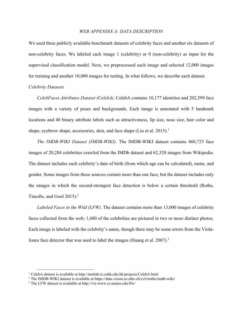
WEB APPENDIX A: DATA DESCRIPTION

We used three publicly available benchmark datasets of celebrity faces and another six datasets of

non-celebrity faces. We labeled each image 1 (celebrity) or 0 (non-celebrity) as input for the

supervised classification model. Next, we preprocessed each image and selected 12,000 images

for training and another 10,000 images for testing. In what follows, we describe each dataset.

Celebrity Datasets

CelebFaces Attributes Dataset (CelebA). CelebA contains 10,177 identities and 202,599 face

images with a variety of poses and backgrounds. Each image is annotated with 5 landmark

locations and 40 binary attribute labels such as attractiveness, lip size, nose size, hair color and

shape, eyebrow shape, accessories, skin, and face shape (Liu et al. 2015).1

The IMDB-WIKI Dataset (IMDB-WIKI). The IMDB-WIKI dataset contains 460,723 face

images of 20,284 celebrities crawled from the IMDb dataset and 62,328 images from Wikipedia.

The dataset includes each celebrity’s date of birth (from which age can be calculated), name, and

gender. Some images from these sources contain more than one face, but the dataset includes only

the images in which the second-strongest face detection is below a certain threshold (Rothe,

Timofte, and Gool 2015).2

Labeled Faces in the Wild (LFW). The dataset contains more than 13,000 images of celebrity

faces collected from the web; 1,680 of the celebrities are pictured in two or more distinct photos.

Each image is labeled with the celebrity’s name, though there may be some errors from the Viola-

Jones face detector that was used to label the images (Huang et al. 2007).3

1 CelebA dataset is available at http://mmlab.ie.cuhk.edu.hk/projects/CelebA.html 2 The IMDB-WIKI dataset is available at https://data.vision.ee.ethz.ch/cvl/rrothe/imdb-wiki/ 3 The LFW dataset is available at http://vis-www.cs.umass.edu/lfw/

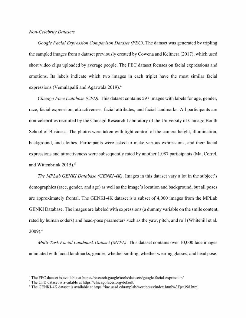
Non-Celebrity Datasets

Google Facial Expression Comparison Dataset (FEC). The dataset was generated by tripling

the sampled images from a dataset previously created by Cowena and Keltnera (2017), which used

short video clips uploaded by average people. The FEC dataset focuses on facial expressions and

emotions. Its labels indicate which two images in each triplet have the most similar facial

expressions (Vemulapalli and Agarwala 2019).4

Chicago Face Database (CFD). This dataset contains 597 images with labels for age, gender,

race, facial expression, attractiveness, facial attributes, and facial landmarks. All participants are

non-celebrities recruited by the Chicago Research Laboratory of the University of Chicago Booth

School of Business. The photos were taken with tight control of the camera height, illumination,

background, and clothes. Participants were asked to make various expressions, and their facial

expressions and attractiveness were subsequently rated by another 1,087 participants (Ma, Correl,

and Wittenbrink 2015).5

The MPLab GENKI Database (GENKI-4K). Images in this dataset vary a lot in the subject’s

demographics (race, gender, and age) as well as the image’s location and background, but all poses

are approximately frontal. The GENKI-4K dataset is a subset of 4,000 images from the MPLab

GENKI Database. The images are labeled with expressions (a dummy variable on the smile content,

rated by human coders) and head-pose parameters such as the yaw, pitch, and roll (Whitehill et al.

2009).6

Multi-Task Facial Landmark Dataset (MTFL). This dataset contains over 10,000 face images

annotated with facial landmarks, gender, whether smiling, whether wearing glasses, and head pose.

4 The FEC dataset is available at https://research.google/tools/datasets/google-facial-expression/ 5 The CFD dataset is available at https://chicagofaces.org/default/ 6 The GENKI-4K dataset is available at https://inc.ucsd.edu/mplab/wordpress/index.html%3Fp=398.html

The dataset was constructed to test the task-constrained deep model proposed by Zhang et al.

(2014), and it contains images from other datasets including Annotated Facial Landmarks in the

Wild (AFLW; Kostinger et al. 2011) and CUHK Face Alignment Database (Wang and Tang 2009).

The images in AFLW are real-world photos of ordinary people; the people vary in ethnicity, age,

gender, clothing, hairstyle, and so on. The images in the CUHK Database feature students at

CUHK (all non-celebrities). MTFL also contains images from LFW, but we removed them so that

our MTFL images feature only non-celebrities. Images are labeled with gender, whether smiling,

whether wearing glasses, head pose, and facial landmarks.7

Selfie Dataset (Selfie). This dataset contains 46,836 selfie images annotated with gender, age,

race, face shape, facial expressions, hair color, hair shape, accessories, and lighting conditions.

Moreover, each image is assigned a popularity score, which indicates attractiveness. The dataset

was constructed by downloading images from selfeed.com, which has real-time updates of

Instagram selfies featuring ordinary people (Kalayeh et al. 2015).8

Flickr-Faces-HQ Dataset (FFHQ). This dataset contains 210,000 images crawled from the

Flickr website. The people in the images vary in age, ethnicity, and background. Workers on

Amazon Mechanical Turk removed images that did not feature faces. There aren’t rich labels for

this dataset (Karras, Samuli, Aila 2019).9

7 The MTFL dataset is available at http://mmlab.ie.cuhk.edu.hk/projects/TCDCN.html 8 The Selfie dataset is available at https://www.crcv.ucf.edu/data/Selfie/ 9 FFHQ data available at https://github.com/NVlabs/ffhq-dataset

WEB APPENDIX B. TECHNICAL NOTES ON THE DEEP LEARNING MODEL FOR

CHARISMA CLASSIFICATION

Backbone Model: ResNet-50

Model structure of the Convolutional Neural Network (CNN). The advantage of a CNN over

a fully connected feedforward neural network lies in the smaller number of free parameters; a CNN

avoids the vanishing gradient and exploding gradient problems that can occur during

backpropagation in traditional neural networks. This advantage is especially crucial for image

classification because each pixel is a variable, so a large set of images represents a prohibitively

large input (Ciregan et al. 2012; Cireşan et al. 2011).

A CNN consists of input and output layers with multiple hidden convolutional layers. The

activation function is followed by convolutions like pooling layers, fully connected layers, and

normalization layers. The input of a CNN is a tensor with shape (number of images) × (image

height) × (image width) × (input channels). After passing through a convolutional layer, the

image is abstracted to a feature map with shape (number of images) × (feature map height) ×

(feature map width) × (feature map channels). Finally, the output is a probability for the category,

typically calculated by a Softmax or Sigmoid function (Gibbs and MacKay 2000).

Convolutional layer. The convolution operation is designed to extract the high-level features

from the input image. The crux of a convolutional layer is the kernel that carries out the

convolution operations by moving to the right with a certain stride value until it parses the whole

matrix. This process is repeated for all channels (images contain three channels: RGB), so the

number of input channels must equal the number of feature map channels.

Pooling Layer. The pooling layer is designed to lessen the computational pressure by reducing

dimensionality and extracting useful features that are unvaried in direction and position while

preserving the effectiveness of the training model. Max Pooling returns the maximum value from

the portion of the image covered by the kernel, while Average Pooling returns the average of all

the values from the portion of the image covered by the kernel.

Fully Connected Layer. As implied by its name, the fully connected layer connects every

neuron in one layer to every neuron in the next layer, which is similar to the mechanism in the

multi-layer perceptron network. Usually, the flattened matrix goes through fully connected layers

and then the final Sigmoid or Softmax layer to classify the images.

ResNet-50: a CNN variant. The Residual Network (ResNet) is proposed to solve the

degradation problem, which is commonly exposed when deep network starts converging. The

ResNet is mainly based on the residual network, where the staked nonlinear layers fit residual

mapping instead of the desired underlying mapping. To be more specific, suppose that the original

mapping is ℋ($), we now consider the residual mapping defined as ℱ($):= ℋ($) − $, which

recast the original mapping into ℱ($) + $. The hypothetical foundation is that pushing the residual

to zero is easier than fitting an identity mapping. Then, the authors apply the short cut connections

which skip layers to achieve the formulation of ℱ($) + $ by feedforward neural networks. One

special thing is that the shortcut connections utilized in this framework do not increase

computational complexity (He et al. 2015; He et al. 2016).

The baseline architecture follows that of VGG nets, in which most convolutional layers have

3 × 3 filters (Simonyan and Zisserman 2015). The architecture requires the output feature map

size to match the number of filters. The time complexity is maintained by doubling the number of

filters if the feature map is halved. Next, down-sampling is conducted with a stride value of 2. The

pooling layer uses global average pooling followed by a fully connected layer and a Softmax layer

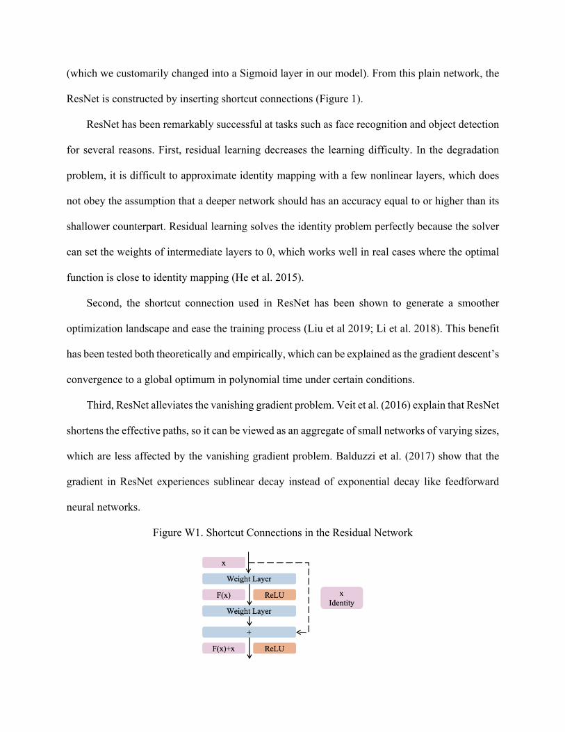
(which we customarily changed into a Sigmoid layer in our model). From this plain network, the

ResNet is constructed by inserting shortcut connections (Figure 1).

ResNet has been remarkably successful at tasks such as face recognition and object detection

for several reasons. First, residual learning decreases the learning difficulty. In the degradation

problem, it is difficult to approximate identity mapping with a few nonlinear layers, which does

not obey the assumption that a deeper network should has an accuracy equal to or higher than its

shallower counterpart. Residual learning solves the identity problem perfectly because the solver

can set the weights of intermediate layers to 0, which works well in real cases where the optimal

function is close to identity mapping (He et al. 2015).

Second, the shortcut connection used in ResNet has been shown to generate a smoother

optimization landscape and ease the training process (Liu et al 2019; Li et al. 2018). This benefit

has been tested both theoretically and empirically, which can be explained as the gradient descent’s

convergence to a global optimum in polynomial time under certain conditions.

Third, ResNet alleviates the vanishing gradient problem. Veit et al. (2016) explain that ResNet

shortens the effective paths, so it can be viewed as an aggregate of small networks of varying sizes,

which are less affected by the vanishing gradient problem. Balduzzi et al. (2017) show that the

gradient in ResNet experiences sublinear decay instead of exponential decay like feedforward

neural networks.

Figure W1. Shortcut Connections in the Residual Network

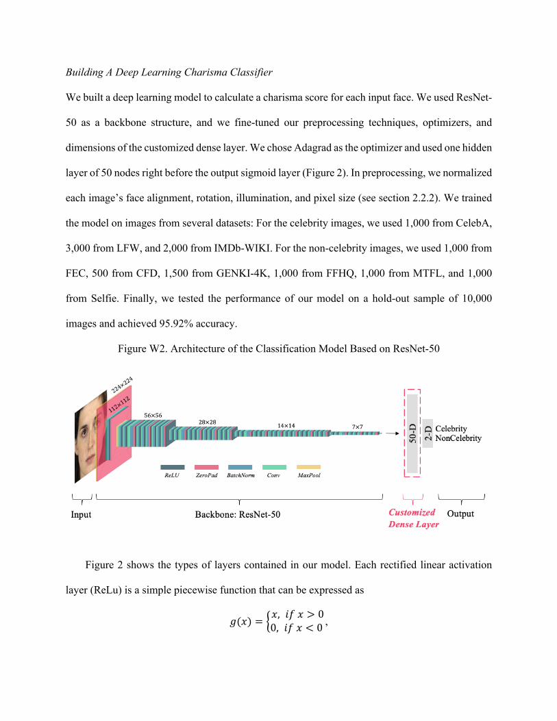
Building A Deep Learning Charisma Classifier

We built a deep learning model to calculate a charisma score for each input face. We used ResNet-

50 as a backbone structure, and we fine-tuned our preprocessing techniques, optimizers, and

dimensions of the customized dense layer. We chose Adagrad as the optimizer and used one hidden

layer of 50 nodes right before the output sigmoid layer (Figure 2). In preprocessing, we normalized

each image’s face alignment, rotation, illumination, and pixel size (see section 2.2.2). We trained

the model on images from several datasets: For the celebrity images, we used 1,000 from CelebA,

3,000 from LFW, and 2,000 from IMDb-WIKI. For the non-celebrity images, we used 1,000 from

FEC, 500 from CFD, 1,500 from GENKI-4K, 1,000 from FFHQ, 1,000 from MTFL, and 1,000

from Selfie. Finally, we tested the performance of our model on a hold-out sample of 10,000

images and achieved 95.92% accuracy.

Figure W2. Architecture of the Classification Model Based on ResNet-50

Figure 2 shows the types of layers contained in our model. Each rectified linear activation

layer (ReLu) is a simple piecewise function that can be expressed as

,($) = -$, /0$ > 00, /0$ < 0,

and is widely used for its computational simplicity and representational sparsity (Glorot, Bordes,

and Bengio 2011). The zero padding layers simply add zeros to the end of a time-domain signal to

increase its length. Batch normalization layers rescale and recenter the input to increase the speed

and stability of the neural network (Sergey and Christian 2015). For explanations of the

convolutional and pooling layers, see Section 2.1.1.

Comparison with other models. Based on previous research, ResNet outperforms AlexNet

(Krizhevsky et al. 2012) and VGG net (Simonyan and Zisserman 2015), thus we only consider

comparing it with SE-ResNet-50 model (Hu et al. 2018), which is built by adding a new unit,

Squeeze-and-Excitation (SE) block, on top of ResNet-50. The SE block is designed to create better

representations, which is realized by allowing for feature recalibration. Such mechanism not only

focuses on informative features, but also suppressed less useful ones, according to global

information. When both ResNet-50 and SE-ResNet-50 are tested on the ImageNet validation set,

SE-ResNet-50 reports slightly lower error, which approaches the deep network ResNet-101.

However, this is achieved by sacrificing the runtime. Besides, this is only the result on a single

dataset, and the same performance may not be happening on different datasets. Thus, to select the

optimal backbone structure, we carefully tested these two models on our dataset. After trying these

two model structures on the same training set using different optimizers, we found that ResNet-50

has better performance. Hence, we decided to adopt it (Table 1).

Preprocessing Techniques. Following the previous literature, we implemented techniques

including face alignment and rotation (Kovenko 2019; Kazemi and Sullivan 2014), illumination

normalization (Zhang et al. 2007; Khayat et al. 2008), rescaling the pixels between 0 and 1, as well

as data augmentation by flipping and tilting the images in the training set (Krizhevsky et al. 2012).

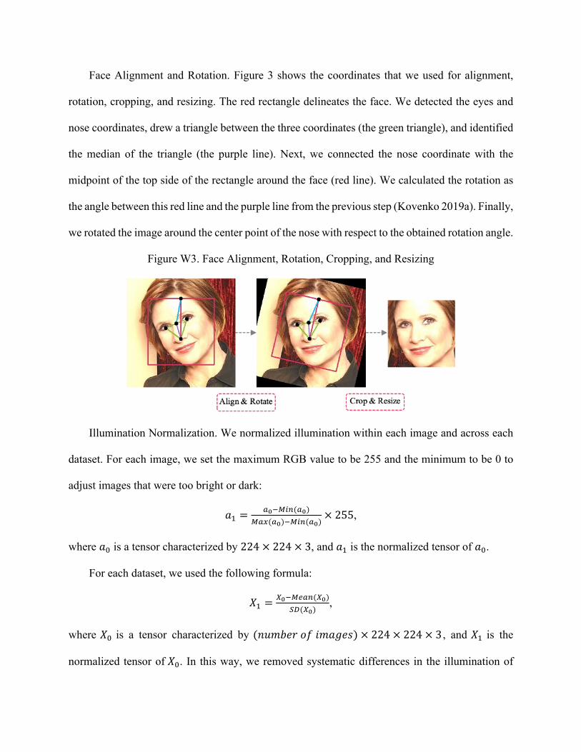
Face Alignment and Rotation. Figure 3 shows the coordinates that we used for alignment,

rotation, cropping, and resizing. The red rectangle delineates the face. We detected the eyes and

nose coordinates, drew a triangle between the three coordinates (the green triangle), and identified

the median of the triangle (the purple line). Next, we connected the nose coordinate with the

midpoint of the top side of the rectangle around the face (red line). We calculated the rotation as

the angle between this red line and the purple line from the previous step (Kovenko 2019a). Finally,

we rotated the image around the center point of the nose with respect to the obtained rotation angle.

Figure W3. Face Alignment, Rotation, Cropping, and Resizing

Illumination Normalization. We normalized illumination within each image and across each

dataset. For each image, we set the maximum RGB value to be 255 and the minimum to be 0 to

adjust images that were too bright or dark:

5! ="!#$%&("!)

$")("!)#$%&("!)× 255,

where 5* is a tensor characterized by 224 × 224 × 3, and 5! is the normalized tensor of 5*.

For each dataset, we used the following formula:

9! =+!#$,"&(+!)

-.(+!),

where 9* is a tensor characterized by (:;<=>?@0/<5,>A) × 224 × 224 × 3 , and 9! is the

normalized tensor of 9*. In this way, we removed systematic differences in the illumination of

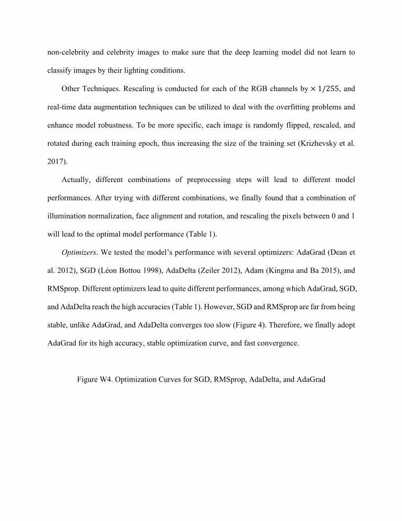
non-celebrity and celebrity images to make sure that the deep learning model did not learn to

classify images by their lighting conditions.

Other Techniques. Rescaling is conducted for each of the RGB channels by × 1/255, and

real-time data augmentation techniques can be utilized to deal with the overfitting problems and

enhance model robustness. To be more specific, each image is randomly flipped, rescaled, and

rotated during each training epoch, thus increasing the size of the training set (Krizhevsky et al.

2017).

Actually, different combinations of preprocessing steps will lead to different model

performances. After trying with different combinations, we finally found that a combination of

illumination normalization, face alignment and rotation, and rescaling the pixels between 0 and 1

will lead to the optimal model performance (Table 1).

Optimizers. We tested the model’s performance with several optimizers: AdaGrad (Dean et

al. 2012), SGD (Léon Bottou 1998), AdaDelta (Zeiler 2012), Adam (Kingma and Ba 2015), and

RMSprop. Different optimizers lead to quite different performances, among which AdaGrad, SGD,

and AdaDelta reach the high accuracies (Table 1). However, SGD and RMSprop are far from being

stable, unlike AdaGrad, and AdaDelta converges too slow (Figure 4). Therefore, we finally adopt

AdaGrad for its high accuracy, stable optimization curve, and fast convergence.

Figure W4. Optimization Curves for SGD, RMSprop, AdaDelta, and AdaGrad

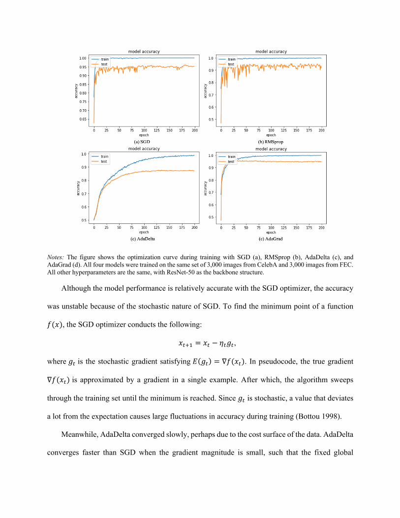
Notes: The figure shows the optimization curve during training with SGD (a), RMSprop (b), AdaDelta (c), and

AdaGrad (d). All four models were trained on the same set of 3,000 images from CelebA and 3,000 images from FEC.

All other hyperparameters are the same, with ResNet-50 as the backbone structure.

Although the model performance is relatively accurate with the SGD optimizer, the accuracy

was unstable because of the stochastic nature of SGD. To find the minimum point of a function

0($), the SGD optimizer conducts the following:

$/0! = $/ − D/,/,

where ,/ is the stochastic gradient satisfying E(,/) = ∇0($/). In pseudocode, the true gradient

∇0($/) is approximated by a gradient in a single example. After which, the algorithm sweeps

through the training set until the minimum is reached. Since ,/ is stochastic, a value that deviates

a lot from the expectation causes large fluctuations in accuracy during training (Bottou 1998).

Meanwhile, AdaDelta converged slowly, perhaps due to the cost surface of the data. AdaDelta

converges faster than SGD when the gradient magnitude is small, such that the fixed global

learning rate shared by all dimensions cannot speed up progress (Zeiler 2012). When the gradient

magnitude is large, however, SGD may converge faster since it can make a big jump at one step.

Customized dense layer, batch, epoch, and training set. Since the original ResNet-50 model

does not fit our classification task, we modified the backbone architecture by adding additional

dense layers and replacing the Softmax layer with a Sigmoid layer for classifying the images into

two categories (celebrity and non-celebrity). We regarded the number of additional dense layers

and the number of neurons within each dense layer as hyperparameters, and tested several

combinations: (i) 512 neurons at layer 1 + 20 neurons at layer 2, (ii) 20 neurons at layer 1 + 512

neurons at layer 2, (iii) 1024 neurons at layer 1 + 20 neurons at layer 2, (iv) one layer with 1000

neurons, (v) one layer with 50 neurons, and (vi) one layer with 20 neurons. We tested each

combination on a set of 6,000 images from CelebA and 6,000 from FEC, and the results are in

Table 1. We chose option (v) for its combination of relatively high accuracy and small size, which

makes it easier to interpret and build connections with the 11 facial features.

For the batch number, we tested 32 and 10. We found that the model performed better with

10 (Table 1). For the number of epochs, we tested 100 and 200. We chose 200 to ensure full

optimization.

Finally, to enhance model robustness across different datasets, we constructed the training and

testing sets from all 9 datasets described in section 1.1. For the celebrity images, we randomly

selected 1,000 from CelebA, 3,000 from LFW, and 2,000 from IMDb-WIKI. For the non-celebrity

images, we randomly selected 1,000 from FEC, 500 from CFD, 1,500 from GENKI-4K, 1,000

from FFHQ, 1,000 from MTFL, and 1,000 from Selfie. Some images contained multiple faces, but

we used only the first face detected, giving us a total of 12,000 faces for training.

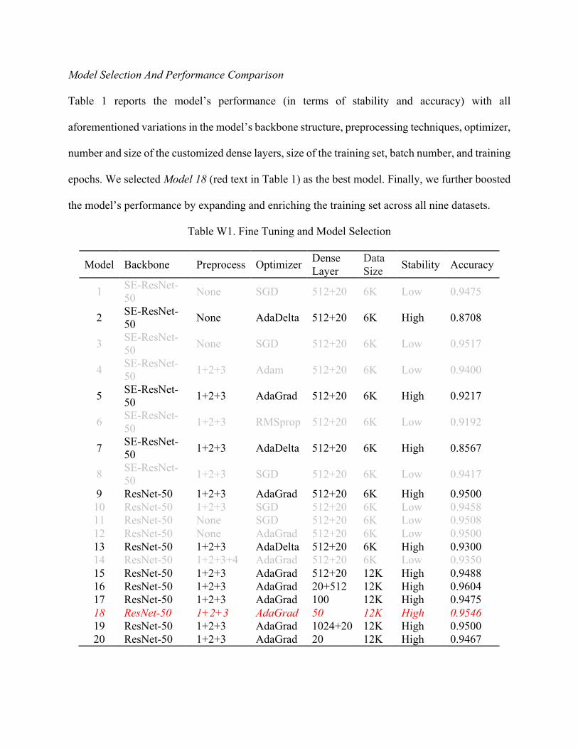
Model Selection And Performance Comparison

Table 1 reports the model’s performance (in terms of stability and accuracy) with all

aforementioned variations in the model’s backbone structure, preprocessing techniques, optimizer,

number and size of the customized dense layers, size of the training set, batch number, and training

epochs. We selected Model 18 (red text in Table 1) as the best model. Finally, we further boosted

the model’s performance by expanding and enriching the training set across all nine datasets.

Table W1. Fine Tuning and Model Selection

Model Backbone Preprocess Optimizer Dense Layer

Data Size Stability Accuracy

1 SE-ResNet-50 None SGD 512+20 6K Low 0.9475

2 SE-ResNet-50 None AdaDelta 512+20 6K High 0.8708

3 SE-ResNet-50 None SGD 512+20 6K Low 0.9517

4 SE-ResNet-50 1+2+3 Adam 512+20 6K Low 0.9400

5 SE-ResNet-50 1+2+3 AdaGrad 512+20 6K High 0.9217

6 SE-ResNet-50 1+2+3 RMSprop 512+20 6K Low 0.9192

7 SE-ResNet-50 1+2+3 AdaDelta 512+20 6K High 0.8567

8 SE-ResNet-50 1+2+3 SGD 512+20 6K Low 0.9417

9 ResNet-50 1+2+3 AdaGrad 512+20 6K High 0.9500 10 ResNet-50 1+2+3 SGD 512+20 6K Low 0.9458 11 ResNet-50 None SGD 512+20 6K Low 0.9508 12 ResNet-50 None AdaGrad 512+20 6K Low 0.9500 13 ResNet-50 1+2+3 AdaDelta 512+20 6K High 0.9300 14 ResNet-50 1+2+3+4 AdaGrad 512+20 6K Low 0.9350 15 ResNet-50 1+2+3 AdaGrad 512+20 12K High 0.9488 16 ResNet-50 1+2+3 AdaGrad 20+512 12K High 0.9604 17 ResNet-50 1+2+3 AdaGrad 100 12K High 0.9475 18 ResNet-50 1+2+3 AdaGrad 50 12K High 0.9546 19 ResNet-50 1+2+3 AdaGrad 1024+20 12K High 0.9500 20 ResNet-50 1+2+3 AdaGrad 20 12K High 0.9467

Notes: The table shows all the models we trained to find the optimal hyperparameters. We had two choices for the

Backbone: ResNet-50 and SE-ResNet-50. In the Preprocessing column, 1 = face alignment and rotation, 2 =

illumination normalization, 3 = rescaling RGB, and 4 = data augmentation. We tested five Optimizers: SGD, AdaDelta,

Adam, AdaGrad, and RMSprop. In the Dense Layer column, the number(s) indicate the neurons in the one or two

dense layers. Data Size is the number of images in the training dataset; regardless of size, half came from CelebA, and

the other half came from FEC. Stability is a binary variable denoting whether the optimization curve during training

was stable (High) or unstable (Low); we considered only the models with high stability, so models with low stability

are printed in gray text. Accuracy is the testing accuracy on the hold-out set.

Overfitting can decrease a model’s performance on the test set and reduce the model’s

generalizability, so we adopted two strategies to avoid overfitting. First, we used batch

normalization, which works well as a method of regularization; dropout has little effect on

overfitting in some batch-normalized networks (Ioffe and Szegedy 2015). If we have < values of

a specific activation $ in the minibatch G = {$!,…, $1},then batch normalization is performed as

follows:

J% = 5 )"#2√4#05 + =,

where K and L6 are the mean and variance of G = {$!,…, $1}, respectively.

Second, we used early stopping, meaning that we ended training before the model became

overfitted. This is one of the oldest and most widely used forms of regularization. We conducted

real-time monitoring with Tensorboard, which tracks the training and testing accuracy at each

epoch during the training process.10 We stopped the training when we observed that the accuracy

curve for the hold-out set began to decline (Bishop 2006).

10 The specific introduction can be viewed at https://www.tensorflow.org/tensorboard.

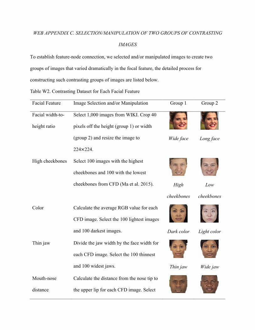
WEB APPENDIX C. SELECTION/MANIPULATION OF TWO GROUPS OF CONTRASTING

IMAGES

To establish feature-node connection, we selected and/or manipulated images to create two

groups of images that varied dramatically in the focal feature, the detailed process for

constructing such contrasting groups of images are listed below.

Table W2. Contrasting Dataset for Each Facial Feature

Facial Feature Image Selection and/or Manipulation Group 1 Group 2

Facial width-to-

height ratio

Select 1,000 images from WIKI. Crop 40

pixels off the height (group 1) or width

(group 2) and resize the image to

224×224.

Wide face

Long face

High cheekbones Select 100 images with the highest

cheekbones and 100 with the lowest

cheekbones from CFD (Ma et al. 2015).

High

cheekbones

Low

cheekbones

Color Calculate the average RGB value for each

CFD image. Select the 100 lightest images

and 100 darkest images.

Dark color

Light color

Thin jaw Divide the jaw width by the face width for

each CFD image. Select the 100 thinnest

and 100 widest jaws.

Thin jaw

Wide jaw

Mouth-nose

distance

Calculate the distance from the nose tip to

the upper lip for each CFD image. Select

the 100 longest and 100 shortest mouth-

nose distances.

Long Short

Large eyes Divide the eye height by the face length for

each CFD image. Select the 100 largest

and 100 smallest eyes.

Large eyes

Small eyes

Sex dimorphism Detect the gender score for each WIKI

image. Select 500 images with a gender

score higher than 0.9 or lower than 0.1,

and 500 images with a gender score

between 0.3 and 0.7.

High

Low

Mouth-chin

distance

Calculate the distance from the bottom

edge of the lower lip to the base of the chin

for each CFD image. Select the 100

longest and 100 shortest mouth-chin

distances.

Long

Short

Babyfaceness Select 100 images with the highest

babyfaceness score and 100 images with

the lowest score from CFD.

High

babyfaceness

Low

babyfaceness

Symmetry Calculate the Euclidean distance between

the right half and left half of the face for

each CFD image. Select the 100 longest

High

symmetry

Low

symmetry

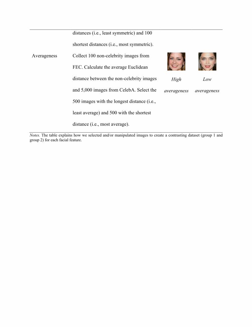
distances (i.e., least symmetric) and 100

shortest distances (i.e., most symmetric).

Averageness Collect 100 non-celebrity images from

FEC. Calculate the average Euclidean

distance between the non-celebrity images

and 5,000 images from CelebA. Select the

500 images with the longest distance (i.e.,

least average) and 500 with the shortest

distance (i.e., most average).

High

averageness

Low

averageness

Notes. The table explains how we selected and/or manipulated images to create a contrasting dataset (group 1 and

group 2) for each facial feature.

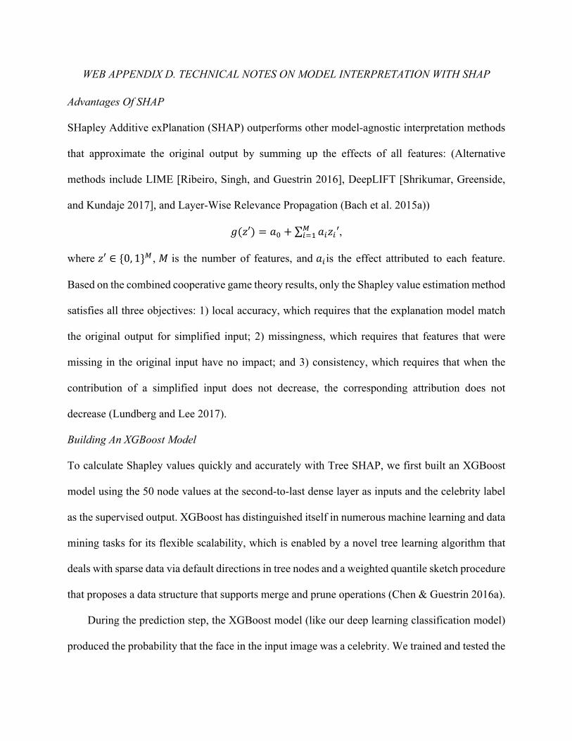
WEB APPENDIX D. TECHNICAL NOTES ON MODEL INTERPRETATION WITH SHAP

Advantages Of SHAP

SHapley Additive exPlanation (SHAP) outperforms other model-agnostic interpretation methods

that approximate the original output by summing up the effects of all features: (Alternative

methods include LIME [Ribeiro, Singh, and Guestrin 2016], DeepLIFT [Shrikumar, Greenside,

and Kundaje 2017], and Layer-Wise Relevance Propagation (Bach et al. 2015a))

,(M′) = 5* + ∑ 5%M%′$%7! ,

where M′ ∈ {0, 1}$ , Q is the number of features, and 5% is the effect attributed to each feature.

Based on the combined cooperative game theory results, only the Shapley value estimation method

satisfies all three objectives: 1) local accuracy, which requires that the explanation model match

the original output for simplified input; 2) missingness, which requires that features that were

missing in the original input have no impact; and 3) consistency, which requires that when the

contribution of a simplified input does not decrease, the corresponding attribution does not

decrease (Lundberg and Lee 2017).

Building An XGBoost Model

To calculate Shapley values quickly and accurately with Tree SHAP, we first built an XGBoost

model using the 50 node values at the second-to-last dense layer as inputs and the celebrity label

as the supervised output. XGBoost has distinguished itself in numerous machine learning and data

mining tasks for its flexible scalability, which is enabled by a novel tree learning algorithm that

deals with sparse data via default directions in tree nodes and a weighted quantile sketch procedure

that proposes a data structure that supports merge and prune operations (Chen & Guestrin 2016a).

During the prediction step, the XGBoost model (like our deep learning classification model)

produced the probability that the face in the input image was a celebrity. We trained and tested the

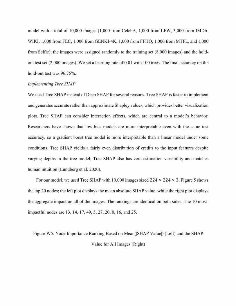
model with a total of 10,000 images (1,000 from CelebA, 1,000 from LFW, 3,000 from IMDb-

WIKI, 1,000 from FEC, 1,000 from GENKI-4K, 1,000 from FFHQ, 1,000 from MTFL, and 1,000

from Selfie); the images were assigned randomly to the training set (8,000 images) and the hold-

out test set (2,000 images). We set a learning rate of 0.01 with 100 trees. The final accuracy on the

hold-out test was 96.75%.

Implementing Tree SHAP

We used Tree SHAP instead of Deep SHAP for several reasons. Tree SHAP is faster to implement

and generates accurate rather than approximate Shapley values, which provides better visualization

plots. Tree SHAP can consider interaction effects, which are central to a model’s behavior.

Researchers have shown that low-bias models are more interpretable even with the same test

accuracy, so a gradient boost tree model is more interpretable than a linear model under some

conditions. Tree SHAP yields a fairly even distribution of credits to the input features despite

varying depths in the tree model; Tree SHAP also has zero estimation variability and matches

human intuition (Lundberg et al. 2020).

For our model, we used Tree SHAP with 10,000 images sized 224 × 224 × 3. Figure 5 shows

the top 20 nodes; the left plot displays the mean absolute SHAP value, while the right plot displays

the aggregate impact on all of the images. The rankings are identical on both sides. The 10 most-

impactful nodes are 13, 14, 17, 49, 5, 27, 20, 0, 16, and 25.

Figure W5. Node Importance Ranking Based on Mean(|SHAP Value|) (Left) and the SHAP

Value for All Images (Right)

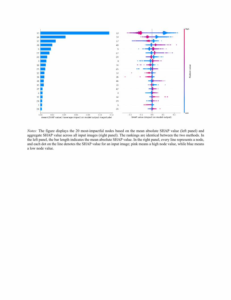
Notes: The figure displays the 20 most-impactful nodes based on the mean absolute SHAP value (left panel) and

aggregate SHAP value across all input images (right panel). The rankings are identical between the two methods. In

the left panel, the bar length indicates the mean absolute SHAP value. In the right panel, every line represents a node,

and each dot on the line denotes the SHAP value for an input image; pink means a high node value, while blue means

a low node value.

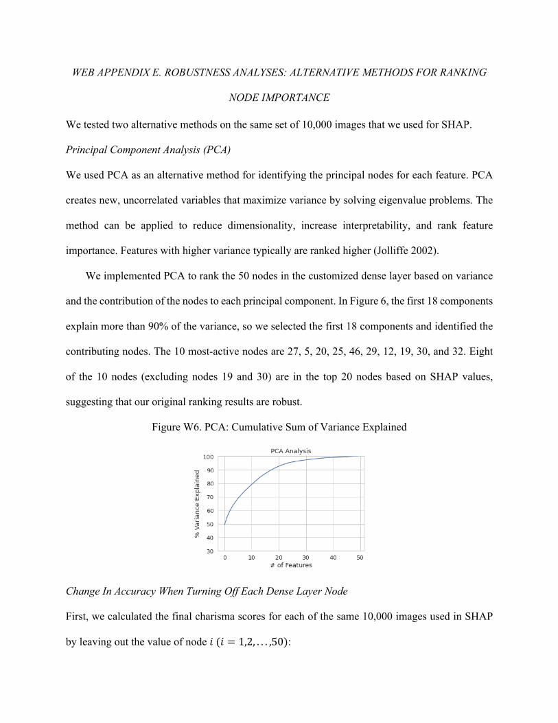
WEB APPENDIX E. ROBUSTNESS ANALYSES: ALTERNATIVE METHODS FOR RANKING

NODE IMPORTANCE

We tested two alternative methods on the same set of 10,000 images that we used for SHAP.

Principal Component Analysis (PCA)

We used PCA as an alternative method for identifying the principal nodes for each feature. PCA

creates new, uncorrelated variables that maximize variance by solving eigenvalue problems. The

method can be applied to reduce dimensionality, increase interpretability, and rank feature

importance. Features with higher variance typically are ranked higher (Jolliffe 2002).

We implemented PCA to rank the 50 nodes in the customized dense layer based on variance

and the contribution of the nodes to each principal component. In Figure 6, the first 18 components

explain more than 90% of the variance, so we selected the first 18 components and identified the

contributing nodes. The 10 most-active nodes are 27, 5, 20, 25, 46, 29, 12, 19, 30, and 32. Eight

of the 10 nodes (excluding nodes 19 and 30) are in the top 20 nodes based on SHAP values,

suggesting that our original ranking results are robust.

Figure W6. PCA: Cumulative Sum of Variance Explained

Change In Accuracy When Turning Off Each Dense Layer Node

First, we calculated the final charisma scores for each of the same 10,000 images used in SHAP

by leaving out the value of node /(/ = 1,2, . . . ,50):

S;?:T@U:_WX@?>% = 0(9¬% , Y) =,)9(∑ )$<$%!

$&',$)" 0=)!0,)9(∑ )$<$%!

$&',$)" 0=),

where 9¬% is a (Z − 1) × 1 vector with elements ($!, $6, . . . , $>) leaving out $% ; Y is a (Z +

1) × 1 vector describing the weight of each node, with Z = 50; X is the bias parameter. Then, we

judged whether this image is correctly classified by comparing its label with this

S;?:T@U:_WX@?>%, and calculated the total classification accuracy across all 10,000 images. The

same procedure was repeated for all 50 nodes, and the accuracy differences before and after turning

down each of 50 nodes are in Figure 7. We found that most active nodes using this method overlap

with the most active nodes based on SHAP ranking, including Node 20, 13, 16, 17, 5, 49, 0, 46,

29, and 15, verifying the reliability of ranking based on SHAP values.

Figure W7. Change in Accuracy When Turning Off Each Node

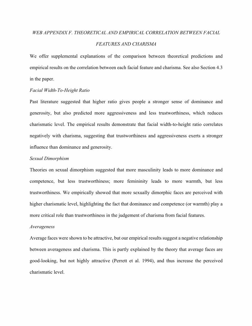
WEB APPENDIX F. THEORETICAL AND EMPIRICAL CORRELATION BETWEEN FACIAL

FEATURES AND CHARISMA

We offer supplemental explanations of the comparison between theoretical predictions and

empirical results on the correlation between each facial feature and charisma. See also Section 4.3

in the paper.

Facial Width-To-Height Ratio

Past literature suggested that higher ratio gives people a stronger sense of dominance and

generosity, but also predicted more aggressiveness and less trustworthiness, which reduces

charismatic level. The empirical results demonstrate that facial width-to-height ratio correlates

negatively with charisma, suggesting that trustworthiness and aggressiveness exerts a stronger

influence than dominance and generosity.

Sexual Dimorphism

Theories on sexual dimorphism suggested that more masculinity leads to more dominance and

competence, but less trustworthiness; more femininity leads to more warmth, but less

trustworthiness. We empirically showed that more sexually dimorphic faces are perceived with

higher charismatic level, highlighting the fact that dominance and competence (or warmth) play a

more critical role than trustworthiness in the judgement of charisma from facial features.

Averageness

Average faces were shown to be attractive, but our empirical results suggest a negative relationship

between averageness and charisma. This is partly explained by the theory that average faces are

good-looking, but not highly attractive (Perrett et al. 1994), and thus increase the perceived

charismatic level.

Symmetry

Past studies proved that symmetric faces look more competent, trustworthy, and attractive, leading

to more charisma, which is in line with our empirical results.

Color

Deeper skin color was perceived with more aggressiveness and dominance. We found that faces

with darker (vs lighter) facial color is associated with a higher (vs lower) charisma level. The

interpretation is that the perceived charisma correlates more with dominance than with

aggressiveness.

Babyfaceness

Babyfaceness was perceived with warmth and trustworthiness, but less dominance and

aggressiveness. Our empirical results suggest that babyfaceness correlates negatively with

charisma. This is a little out of expectation, since three personality traits have positive effect and

only one trait has a negative effect. The explanation might be that the effect of dominance is

stronger than the total influence of warmth, trustworthiness, and aggressiveness.

High Cheekbones

Researchers have shown that people with high cheekbones are perceived with more competence,

leading to more charisma, and our result verifies this hypothesis.

Eye Size

Prior research suggested that large eye size corelates positively to warmth, trustworthiness, and

attractiveness, but reduces dominance. Our empirical result shows that eye size correlates

positively to charismatic level, which may be explained by the fact that three traits affected by

large eyes contribute positively, while only one trait contributes negatively to charisma.

Thin Jaw

A thin jaw was theoretically associated with less dominance and aggressiveness. We empirically

resolved the tension between these features by showing that thin jaw correlates positively with

charisma, indicating that aggressiveness outweighs dominance in contributing to the perceived

charisma.

Mouth-Chin Distance

Past studies have shown that longer mouth-chin distance brings more perceived dominance and

competence, but less physical attractiveness, while the empirical results show that it contributes

positively to charisma. This denotes that the effect of dominance and competence is larger than

that of attractiveness.

Mouth-Nose Distance

Scholars argued that long mouth-nose distance leads to more aggressiveness, but less competence

and physical attractiveness. Therefore, we hypothesized that this feature relates negatively with

charisma. Our result confirms such conjecture.

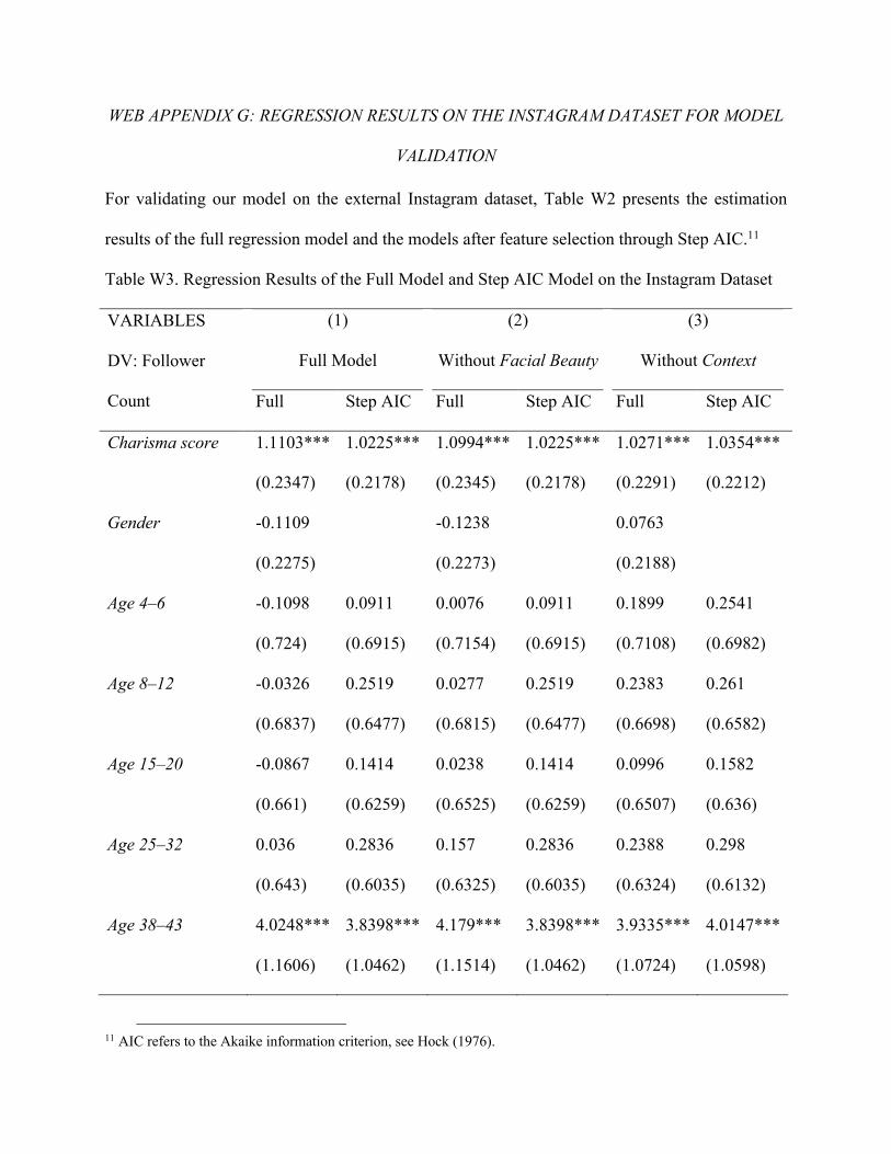
WEB APPENDIX G: REGRESSION RESULTS ON THE INSTAGRAM DATASET FOR MODEL

VALIDATION

For validating our model on the external Instagram dataset, Table W2 presents the estimation

results of the full regression model and the models after feature selection through Step AIC.11

Table W3. Regression Results of the Full Model and Step AIC Model on the Instagram Dataset

VARIABLES

DV: Follower

Count

(1)

Full Model

(2)

Without Facial Beauty

(3)

Without Context

Full Step AIC Full Step AIC Full Step AIC

Charisma score 1.1103*** 1.0225*** 1.0994*** 1.0225*** 1.0271*** 1.0354***

(0.2347) (0.2178) (0.2345) (0.2178) (0.2291) (0.2212)

Gender -0.1109 -0.1238 0.0763

(0.2275) (0.2273) (0.2188)

Age 4–6 -0.1098 0.0911 0.0076 0.0911 0.1899 0.2541

(0.724) (0.6915) (0.7154) (0.6915) (0.7108) (0.6982)

Age 8–12 -0.0326 0.2519 0.0277 0.2519 0.2383 0.261

(0.6837) (0.6477) (0.6815) (0.6477) (0.6698) (0.6582)

Age 15–20 -0.0867 0.1414 0.0238 0.1414 0.0996 0.1582

(0.661) (0.6259) (0.6525) (0.6259) (0.6507) (0.636)

Age 25–32 0.036 0.2836 0.157 0.2836 0.2388 0.298

(0.643) (0.6035) (0.6325) (0.6035) (0.6324) (0.6132)

Age 38–43 4.0248*** 3.8398*** 4.179*** 3.8398*** 3.9335*** 4.0147***

(1.1606) (1.0462) (1.1514) (1.0462) (1.0724) (1.0598)

11 AIC refers to the Akaike information criterion, see Hock (1976).

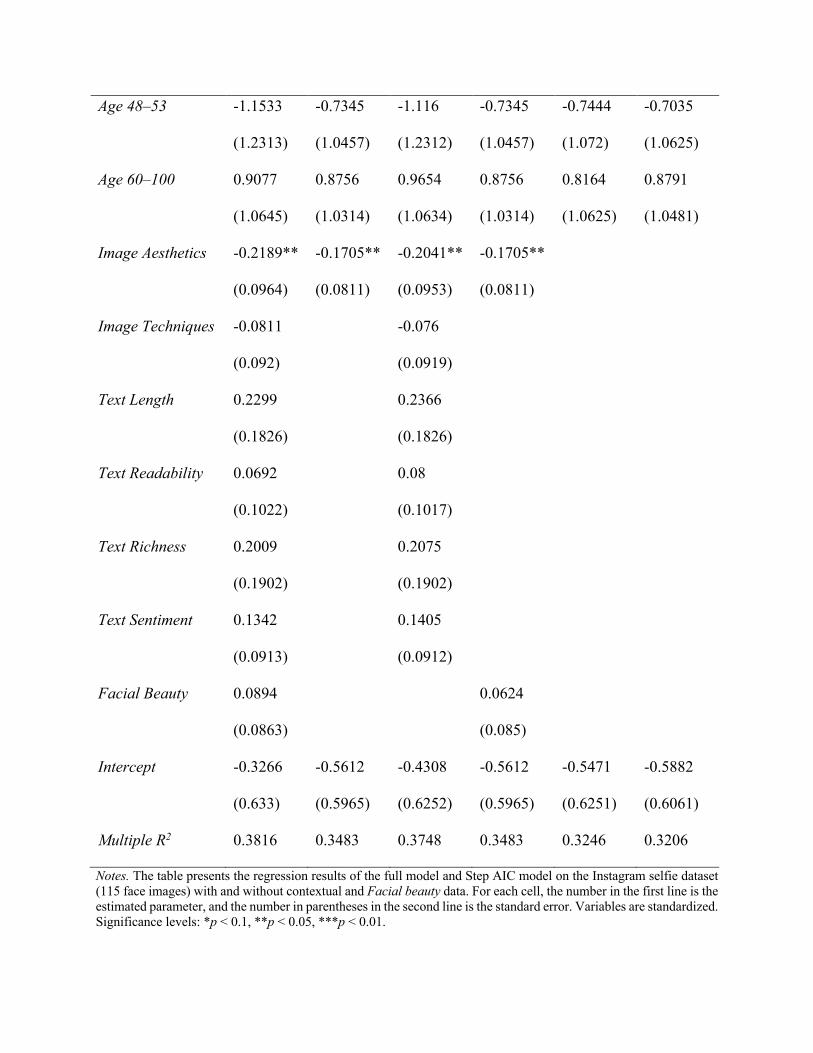
Age 48–53 -1.1533 -0.7345 -1.116 -0.7345 -0.7444 -0.7035

(1.2313) (1.0457) (1.2312) (1.0457) (1.072) (1.0625)

Age 60–100 0.9077 0.8756 0.9654 0.8756 0.8164 0.8791

(1.0645) (1.0314) (1.0634) (1.0314) (1.0625) (1.0481)

Image Aesthetics -0.2189** -0.1705** -0.2041** -0.1705**

(0.0964) (0.0811) (0.0953) (0.0811)

Image Techniques -0.0811 -0.076

(0.092) (0.0919)

Text Length 0.2299 0.2366

(0.1826) (0.1826)

Text Readability 0.0692 0.08

(0.1022) (0.1017)

Text Richness 0.2009 0.2075

(0.1902) (0.1902)

Text Sentiment 0.1342 0.1405

(0.0913) (0.0912)

Facial Beauty 0.0894 0.0624

(0.0863) (0.085)

Intercept -0.3266 -0.5612 -0.4308 -0.5612 -0.5471 -0.5882

(0.633) (0.5965) (0.6252) (0.5965) (0.6251) (0.6061)

Multiple R2 0.3816 0.3483 0.3748 0.3483 0.3246 0.3206

Notes. The table presents the regression results of the full model and Step AIC model on the Instagram selfie dataset

(115 face images) with and without contextual and Facial beauty data. For each cell, the number in the first line is the

estimated parameter, and the number in parentheses in the second line is the standard error. Variables are standardized.

Significance levels: *p < 0.1, **p < 0.05, ***p < 0.01.

REFERENCES

Bach, Sebastian, Alexander Binder, Grégoire Montavon, Frederick Klauschen, Klaus-Robert

Müller, and Wojciech Samek (2015), “On Pixel-Wise Explanations for Non-Linear Classifier

Decisions by Layer-Wise Relevance Propagation,” PLOS ONE, 10 (7), e0130140-.

Balduzzi, D, Marcus Frean, Lennox Leary, J P Lewis, Kurt Wan-Duo Ma, and Brian McWilliams

(2017), “The Shattered Gradients Problem: If resnets are the answer, then what is the

question?,” ArXiv, abs/1702.08591.

Bishop, Christopher M. (2006), Pattern Recognition and Machine Learning, New York: Springer-

Verlag New York.

Bottou, L (1999), “On-line learning and stochastic approximations.”

Chen, Tianqi and Carlos Guestrin (2016), “XGBoost: A Scalable Tree Boosting System,” in

Proceedings of the 22nd ACM SIGKDD International Conference on Knowledge Discovery

and Data Mining, KDD ’16, New York, NY, USA: Association for Computing Machinery,

785–94.

Ciregan, D, U Meier, and J Schmidhuber (2012), “Multi-column deep neural networks for image

classification,” in 2012 IEEE Conference on Computer Vision and Pattern Recognition,

3642–49.

Cireşan, Dan C, Ueli Meier, Jonathan Masci, Luca M Gambardella, and Jürgen Schmidhuber

(2011), “Flexible, High Performance Convolutional Neural Networks for Image

Classification,” in Proceedings of the Twenty-Second International Joint Conference on

Artificial Intelligence - Volume Volume Two, IJCAI’11, AAAI Press, 1237–42.

Cowen, Alan S and Dacher Keltner (2017), “Self-report captures 27 distinct categories of emotion

bridged by continuous gradients.,” Proceedings of the National Academy of Sciences of the

United States of America, 114 (38), E7900–7909.

Dean, Jeffrey, Greg Corrado, Rajat Monga, Kai Chen, Matthieu Devin, Mark Mao, Marc aurelio

Ranzato, Andrew Senior, Paul Tucker, Ke Yang, Quoc Le, and Andrew Ng (2012), “Large

Scale Distributed Deep Networks,” in Advances in Neural Information Processing Systems,

F. Pereira, C. J. C. Burges, L. Bottou, and K. Q. Weinberger, eds., Curran Associates, Inc.

Gibbs, M N and D J C Mackay (2000), “Variational Gaussian process classifiers,” IEEE

Transactions on Neural Networks, 11 (6), 1458–64.

Glorot, Xavier, Antoine Bordes, and Yoshua Bengio (2011), “Deep Sparse Rectifier Neural

Networks,” in AISTATS.

He, K, X Zhang, S Ren, and J Sun (2016), “Deep Residual Learning for Image Recognition,” in

2016 IEEE Conference on Computer Vision and Pattern Recognition (CVPR), 770–78.

He, Kaiming, Xiangyu Zhang, Shaoqing Ren, and Jian Sun (2016), Identity Mappings in Deep

Residual Networks.

Hu, Jie, Li Shen, and Gang Sun (2018), “Squeeze-and-Excitation Networks,” in 2018 IEEE/CVF

Conference on Computer Vision and Pattern Recognition, 7132–41.

Huang, Gary, Marwan Mattar, Tamara Berg, and Eric Learned-Miller (2008), “Labeled Faces in

the Wild: A Database forStudying Face Recognition in Unconstrained Environments,” Tech.

rep.

Ioffe, Sergey and Christian Szegedy (2015), “Batch Normalization: Accelerating Deep Network

Training by Reducing Internal Covariate Shift,” in Proceedings of the 32nd International

Conference on International Conference on Machine Learning - Volume 37, ICML’15,

JMLR.org, 448–56.

Jolliffe, I. T. (2002), Principal Component Analysis, New York: Springer-Verlag.

Kalayeh, Mahdi M, Misrak Seifu, Wesna LaLanne, and Mubarak Shah (2015), “How to Take a

Good Selfie?,” in Proceedings of the 23rd ACM International Conference on Multimedia,

MM ’15, New York, NY, USA: Association for Computing Machinery, 923–26.

Karras, Tero, Samuli Laine, and Timo Aila (2019), “A Style-Based Generator Architecture for

Generative Adversarial Networks,” in 2019 IEEE/CVF Conference on Computer Vision and

Pattern Recognition (CVPR), 4396–4405.

Kazemi, Vahid and Josephine Sullivan (2014), “One millisecond face alignment with an ensemble

of regression trees,” in 2014 IEEE Conference on Computer Vision and Pattern Recognition,

1867–74.

Khayat, Omid, Hamid Reza Shahdoosti, and Ahmad Jaberi Motlagh (2008), “An Overview on

Model-Based Approaches in Face Recognition,” in Proceedings of the 7th WSEAS

International Conference on Artificial Intelligence, Knowledge Engineering and Data Bases,

AIKED’08, Stevens Point, Wisconsin, USA: World Scientific and Engineering Academy and

Society (WSEAS), 109–15.

Kingma, Diederik P and Jimmy Ba (2015), “Adam: A Method for Stochastic Optimization,” CoRR,

abs/1412.6980.

Köstinger, Martin, Paul Wohlhart, Peter M Roth, and Horst Bischof (2011), “Annotated Facial

Landmarks in the Wild: A large-scale, real-world database for facial landmark localization,”

in 2011 IEEE International Conference on Computer Vision Workshops (ICCV Workshops),

2144–51.

Kovenko, Volodymyr (2019), “How to precisely align face in Python with OpenCv and Dlib,”

Medium.

Krizhevsky, Alex, Ilya Sutskever, and Geoffrey E Hinton (2017), “ImageNet Classification with

Deep Convolutional Neural Networks,” Commun. ACM, 60 (6), 84–90.

Li, Hao, Zheng Xu, G Taylor, and T Goldstein (2018), “Visualizing the Loss Landscape of Neural

Nets,” in NeurIPS.

Liu, Tianyi, Minshuo Chen, Mo Zhou, S Du, Enlu Zhou, and T Zhao (2019), “Towards

Understanding the Importance of Shortcut Connections in Residual Networks,” in NeurIPS.

Liu, Ziwei, Ping Luo, Xiaogang Wang, and Xiaoou Tang (2015), “Deep Learning Face Attributes

in the Wild,” 2015 IEEE International Conference on Computer Vision (ICCV), 3730–38.

Lundberg, Scott M, Gabriel Erion, Hugh Chen, Alex DeGrave, Jordan M Prutkin, Bala Nair, Ronit

Katz, Jonathan Himmelfarb, Nisha Bansal, and Su-In Lee (2020), “From local explanations

to global understanding with explainable AI for trees,” Nature Machine Intelligence, 2 (1),

56–67.

Lundberg, Scott M and Su-In Lee (2017), “A Unified Approach to Interpreting Model Predictions,”

in Proceedings of the 31st International Conference on Neural Information Processing

Systems, NIPS’17, Red Hook, NY, USA: Curran Associates Inc., 4768–77.

Ma, Debbie S, Joshua Correll, and B Wittenbrink (2015), “The Chicago face database: A free

stimulus set of faces and norming data,” Behavior Research Methods, 47, 1122–35.

Ribeiro, Marco, Sameer Singh, and Carlos Guestrin (2016), “Why Should I Trust You?”:

Explaining the Predictions of Any Classifier.

Rothe, Rasmus, Radu Timofte, and Luc van Gool (2015), “DEX: Deep EXpectation of Apparent

Age from a Single Image,” in 2015 IEEE International Conference on Computer Vision

Workshop (ICCVW), 252–57.

Shrikumar, Avanti, Peyton Greenside, and Anshul Kundaje (2017), “Learning Important Features

through Propagating Activation Differences,” in Proceedings of the 34th International

Conference on Machine Learning - Volume 70, ICML’17, JMLR.org, 3145–53.

Simonyan, K and Andrew Zisserman (2015), “Very Deep Convolutional Networks for Large-Scale

Image Recognition,” CoRR, abs/1409.1556.

Veit, Andreas, Michael Wilber, and Serge Belongie (2016), “Residual Networks Behave like

Ensembles of Relatively Shallow Networks,” in Proceedings of the 30th International

Conference on Neural Information Processing Systems, NIPS’16, Red Hook, NY, USA:

Curran Associates Inc., 550–58.

Vemulapalli, Raviteja and Aseem Agarwala (2019), A Compact Embedding for Facial Expression

Similarity.

Wang, Xiaogang and Xiaoou Tang (2009), “Face Photo-Sketch Synthesis and Recognition,” IEEE

Transactions on Pattern Analysis and Machine Intelligence, 31 (11), 1955–67.

Whitehill, Jacob, Marian Bartlett, and Javier Movellan (2008), “Automatic facial expression

recognition for intelligent tutoring systems,” in 2008 IEEE Computer Society Conference on

Computer Vision and Pattern Recognition Workshops, 1–6.

Zeiler, Matthew (2012), “ADADELTA: An adaptive learning rate method,” 1212.

Zhang, Baochang, Shiguang Shan, Xilin Chen, and Wen Gao (2007), “Histogram of Gabor Phase

Patterns (HGPP): A Novel Object Representation Approach for Face Recognition,” IEEE

Transactions on Image Processing, 16 (1), 57–68.