An Acoustic Analysis of Vowel Pronunciation in Swedish ...
256
University of Groningen An Acoustic Analysis of Vowel Pronunciation in Swedish Dialects Leinonen, Therese IMPORTANT NOTE: You are advised to consult the publisher's version (publisher's PDF) if you wish to cite from it. Please check the document version below. Document Version Publisher's PDF, also known as Version of record Publication date: 2010 Link to publication in University of Groningen/UMCG research database Citation for published version (APA): Leinonen, T. (2010). An Acoustic Analysis of Vowel Pronunciation in Swedish Dialects. s.n. Copyright Other than for strictly personal use, it is not permitted to download or to forward/distribute the text or part of it without the consent of the author(s) and/or copyright holder(s), unless the work is under an open content license (like Creative Commons). The publication may also be distributed here under the terms of Article 25fa of the Dutch Copyright Act, indicated by the “Taverne” license. More information can be found on the University of Groningen website: https://www.rug.nl/library/open-access/self-archiving-pure/taverne- amendment. Take-down policy If you believe that this document breaches copyright please contact us providing details, and we will remove access to the work immediately and investigate your claim. Downloaded from the University of Groningen/UMCG research database (Pure): http://www.rug.nl/research/portal. For technical reasons the number of authors shown on this cover page is limited to 10 maximum. Download date: 25-08-2022
-
Upload
khangminh22 -
Category
Documents
-
view
2 -
download
0
Transcript of An Acoustic Analysis of Vowel Pronunciation in Swedish ...

University of Groningen
An Acoustic Analysis of Vowel Pronunciation in Swedish DialectsLeinonen, Therese
IMPORTANT NOTE: You are advised to consult the publisher's version (publisher's PDF) if you wish to cite fromit. Please check the document version below.
Document VersionPublisher's PDF, also known as Version of record
Publication date:2010
Link to publication in University of Groningen/UMCG research database
Citation for published version (APA):Leinonen, T. (2010). An Acoustic Analysis of Vowel Pronunciation in Swedish Dialects. s.n.
CopyrightOther than for strictly personal use, it is not permitted to download or to forward/distribute the text or part of it without the consent of theauthor(s) and/or copyright holder(s), unless the work is under an open content license (like Creative Commons).
The publication may also be distributed here under the terms of Article 25fa of the Dutch Copyright Act, indicated by the “Taverne” license.More information can be found on the University of Groningen website: https://www.rug.nl/library/open-access/self-archiving-pure/taverne-amendment.
Take-down policyIf you believe that this document breaches copyright please contact us providing details, and we will remove access to the work immediatelyand investigate your claim.
Downloaded from the University of Groningen/UMCG research database (Pure): http://www.rug.nl/research/portal. For technical reasons thenumber of authors shown on this cover page is limited to 10 maximum.
Download date: 25-08-2022
An Acoustic Analysis of Vowel
Pronunciation in Swedish Dialects
Therese Leinonen

The work in this thesis has been carried out under the auspices of the NetherlandsNational Graduate School of Linguistics (LOT�Landelijke Onderzoekschool Taal-wetenschap) and the Center for Language and Cognition Groningen (CLCG) of theFaculty of Arts of the University of Groningen.
The work was carried out within the project Determinants of Dialectal Variation�nanced by the Netherlands Organisation for Scienti�c Research�NWO
Groningen Dissertations in Linguistics 83ISSN 0928-0030
ISBN 978-90-367-4450-8c© Therese Leinonen 2010
Cover design: Peter SandbergDocument prepared with LATEX2ε and typeset in pdfTEX
Rijksuniversiteit Groningen
An Acoustic Analysis of Vowel
Pronunciation in Swedish Dialects
Proefschrift
ter verkrijging van het doctoraat in deLetteren
aan de Rijksuniversiteit Groningenop gezag van de
Rector Magni�cus, dr. F. Zwarts,in het openbaar te verdedigen op
donderdag 1 juli 2010om 13.15 uur
door
Therese Nanette Leinonen
geboren op 30 augustus 1976te Vanda, Finland

Promotores: Prof.dr.ir. J. NerbonneProf.dr. V. J. van Heuven
Copromotor: Dr. C. Gooskens
Beoordelingscommissie: Prof.dr. A. ErikssonProf.dr. S. KürschnerProf.dr.ir. L. C. W. PolsProf.dr. M. Thelander

Acknowledgments
Writing this thesis would not have been possible without the help and supportfrom many other people. First of all I would like to thank my three supervisors,John Nerbonne, Vincent van Heuven, and Charlotte Gooskens. My two promotors,John and Vincent, represent two di�erent scienti�c �elds, both of which have beenextremely important for this thesis. John established the dialectometric researchgroup in Groningen, and without all the previous work that has been done withinthis group in Groningen and without the software that has been developed, writingthis thesis would have been impossible. I am also very happy to have had Vincentas my second promotor to support me with the phonetic part of this work. Since theUniversity of Groningen does not have a department of phonetics, it has been veryimportant for me to be able to discuss the phonetic analyses with Vincent (LeidenUniversity).
The support of my co-promotor and daily supervisor, Charlotte, has been invalu-able. Charlotte has read and commented on numerous drafts of all my papers andthe manuscript of the thesis throughout my period as a PhD student. Whenever Ineeded help she could always �nd the time to talk with me. And in di�cult timeswhen I felt that my work was heading into a dead end, a short talk with Char-lotte was always enough to �ll me with new ideas and positive thinking. WithoutCharlotte's guidance and here genuinely positive character the road to �nishing thisthesis would have been much harder to walk.
I am thankful that Anders Eriksson, Sebastian Kürschner, Louis Pols and MatsThelander agreed to be part of the reading committee. Their comments have im-proved the quality of this thesis considerably. I would also like to thank three an-onymous reviewers of my paper in the International Journal of Humanities and ArtsComputing for early on getting valuable comments on work related to my thesis.
I am grateful to have been a member of a research project �nanced by NWOduring my period as a PhD student and to bene�t from a Ubbo Emmius scholarshipfrom the University in Groningen. For �nancial support for printing this thesis I amthankful to the Swedish Cultural Foundation in Finland.
The most important persons for this thesis are the more than 1,000 dialect speak-ers who have participated in the recordings and patiently answered all the questionsfrom the �eldworkers. I have had full and free access to all these dialect data in theSweDia database. I am very grateful to the whole SweDia project, all the dialect
vi
speakers, the �eldworkers, and the people who have segmented and transcribed thedata. I especially want to thank Anders Eriksson for providing me with the data,Eva Sundberg and Margareta Södergård for sharing their experiences from the �eld-work with me, Jonas Lindh for helping me with conversions and Praat scripting,and Anna Ericsson and Cecilia Yttergren for segmenting the last parts of the datafor me during a few hectic summer months in 2009.
When I �rst arrived in Groningen I was very lucky to get to share the o�cewith one cartographer and one dialectometrist. What could have been a betterenvironment for starting the work on a dissertation on dialect geography? JackyBenavides andWilbert Heeringa, thank you for introducing me both to the universityand to your �elds of expertise! Jacky provided me with the geographic coordinatesthat I have used for making all the maps in this book. After all the work with gettingthe coordinates in the right format we could conclude that if Finland is The Land ofthe Thousand Lakes, the Swedish-language parts of Finland surely are The Land ofthe Thousand Islands. I am thankful to Wilbert for introducing me to his work andshowing me how to use the dialectometric software developed in Groningen. I alsoremember all the discussions about statistics that the three of us had in our o�ce.
I am happy to have been able to share my experiences from the work on thisthesis with the dialectometric research group in Groningen. All the discussions andthe support during our meetings have been invaluable, and I would like to thankthe varying members of the group over the years: Charlotte Gooskens, WilbertHeeringa, Sebastian Kürschner, Jens Moberg, John Nerbonne, Jelena Proki¢ andMartijn Wieling. I would especially like to thank Jelena for our numerous discus-sions about clustering, MDS, factor analysis, mapping etc., and for running the Gapanalyses of my data. I would also like to thank Peter Kleiweg who is the program-mer of the L04 software and has made it freely available. Peter helped me withinitial conversions of my data and has been very helpful with promptly making newadditions to the software that I needed for my work.
When I came to Groningen I did not have much knowledge about computationallinguistics. Without all the skills that I have learned from my colleagues I couldnot have �nished this thesis. I would like to thank Lonneke van der Plas and GeertKloosterman for teaching me basic Unix and text manipulation, Tim Van de Cruysand Begoña Villada for teaching corpus linguistics and programming in Perl, JensMoberg for helping me with learning to write in LaTeX, Erik Tjong Kim Sang forgiving a course in statistics in R, and Maartje Schreuder who introduced me tothe Praat software for phonetics. I would also like to thank all the colleagues inthe computational linguistics department for the warm and welcoming internationalsphere.
I would like to thank my student mentor Simone Steenbeek for introducing me tolife in Groningen. For acquiring the Dutch language and learning about the Dutchculture I would like to thank especially Margaret van der Kamp at the LanguageCenter of the University of Groningen, Wendy Prins, and all the members of Gruno'sTNT postharmonie.

vii
After my �rst year in Groningen I got an o�ce in the Scandinavian department.I have enjoyed to be able to discuss the more language-speci�c questions of myresearch with the colleagues in the Scandinavian department, and I would like tothank especially my roommates Sebastian Kürschner, Anja Schüppert, and NannaHaug Hilton.
Contacts outside Groningen have also been very important in the work on thisthesis. Vincent encouraged me to contact Irene Jacobi at the University of Amster-dam to hear about the acoustic method she was using in her work on variation inDutch vowel pronunciation. I am very thankful to Irene for sharing her experienceswith the method and for patiently answering all my questions about Bark �lteringand PCA.
I would like to thank the department of phonetics at the LMU Munich (Ludwig-Maximilians-Universität München) for a short but very intensive visit in July 2008.I was glad about the warm welcome and about the great interest in the work that isbeing done in Groningen. I would like to thank in particular Jonathan Harringtonfor discussing phonetic analysis of vowels with me and for suggesting that I could tryto apply PCA separately on data from male and female speakers. I would also liketo thank Lasse Bombien, Tina John and Michel Sche�ers for support with the EMUSpeech Database System and for a module which enabled me to do the formantanalysis of my data in EMU.
Since we share the same research topic, Swedish vowels, I am very glad to havemet Lena Wenner at a number of conferences and been able to talk to her aboutmy results. She once asked me if it was possible for me to make a mapping of thepronunciation of the Swedish short ö based on my data, which made me come upwith the idea of the maps that are now included in Appendix C of this thesis.
There are many people back home in Finland that I would like to mention. Twopersons are very much responsible for the fact that I applied for a PhD position inGroningen: Leila Mattfolk and Jan-Ola Östman. Leila was the one who saw theadvertisement for a position in a project called Determinants of Dialectal Variationand encouraged me to apply for it because she thought it would �t my researchinterests very well (which it did!). I would like to thank Jan-Ola for talking aboutthe application and my initial research plan with me.
I am glad for the basic research skills that I acquired during my studies at theUniversity of Helsinki and at the Swedish School of Economics and Business Admin-istration in Helsinki. I would like to thank the supervisors of my master's thesis,Marika Tandefelt and Ann-Marie Ivars. I would also like to thank all my formercolleagues at the dictionary of Swedish dialects in Finland (Ordbok över Finlandssvenska folkmål) at the Research Institute for the Languages of Finland: SusanneBergström, Caroline Sandström, Peter Slotte and Carola Åkerlund. Working withthe dictionary was a real pleasure and very instructive for me and has given mevaluable insights in dialectology. Since I have not conducted any �eldwork to gatherdata for this thesis myself, I am happy to have got a little bit of experience of dia-lectological �eldwork from another dialect project: Spara det �nlandssvenska talet.

viii
Having a regional standard variety of Swedish as my �rst language, I am veryhappy about the time I have spent with Ingela Wikman and her family and friendsin Kronoby. The knowledge of a well-preserved rural Swedish dialect that I acquiredthere has made me a better dialectologist.
In Groningen I did not always have access to all of the Swedish dialectologicalliterature. For checking and sending papers to me that I, sometimes very urgently,needed I would like to thank Helga Hilmisdóttir, Lisa Södergård, Lena Wenner, andCarola Åkerlund.
I am deeply thankful to all those who have read and commented on all of or partsof the manuscript of this thesis. My supervisors and the reading committee havealready been mentioned. Others who have read and given useful comments are KarinBeijering, Dicky Gilbers, Nanna Haug Hilton, Julia Klitsch, Jelena Proki¢, AnjaSchüppert, Marika Tandefelt, Lena Wenner, and Martijn Wieling. A special thanksto Nanna for proofreading the whole thesis. All errors and problems remaining inthe text are of course the full responsibility of the author.
I am very happy to have Karin Beijering and Diana Dimitrova at my side duringthe defense of my dissertation. Thank you for being my paranimfs and for supportingme on the big day!
Last but not least I would like to thank all my friends and my family for theirsupport. Tinni, mamma, pappa, tack för att ni har funnits där för mig också om detibland har känts som att jag är hemskt långt borta! Danke auch an meine deutscheFamilie für das warme Willkommen und dass ich als Teil der Familie aufgenommenbin.
Liebes Julchen, danke für deine Liebe!
Berlin, May 15th 2010

Contents
1 Introduction 1
1.1 General motivation . . . . . . . . . . . . . . . . . . . . . . . . . . . . 11.2 Terminology . . . . . . . . . . . . . . . . . . . . . . . . . . . . . . . . 21.3 Overview of the thesis . . . . . . . . . . . . . . . . . . . . . . . . . . 3
2 Background 5
2.1 Swedish dialects and standard language . . . . . . . . . . . . . . . . 52.1.1 Standard Swedish . . . . . . . . . . . . . . . . . . . . . . . . 62.1.2 From dialect diversity to leveled dialects . . . . . . . . . . . . 7
2.2 Swedish dialect geography . . . . . . . . . . . . . . . . . . . . . . . . 102.2.1 Classi�cation of Swedish rural dialects . . . . . . . . . . . . . 122.2.2 Regional varieties of Standard Swedish . . . . . . . . . . . . . 152.2.3 Typologies based on speci�c features . . . . . . . . . . . . . . 15
2.3 Swedish vowels . . . . . . . . . . . . . . . . . . . . . . . . . . . . . . 162.3.1 The Standard Swedish vowel system . . . . . . . . . . . . . . 162.3.2 Regional variation in vowel pronunciation . . . . . . . . . . . 19
2.3.2.1 South Swedish diphthongization . . . . . . . . . . . 192.3.2.2 East Central Swedish diphthongization . . . . . . . 192.3.2.3 Gotlandic diphthongization . . . . . . . . . . . . . . 202.3.2.4 Semi-vowel/fricative ending in long close vowels . . 202.3.2.5 Damped i and y . . . . . . . . . . . . . . . . . . . . 202.3.2.6 Long and short e and ä . . . . . . . . . . . . . . . . 212.3.2.7 Long and short u and ö . . . . . . . . . . . . . . . . 212.3.2.8 The open allophones of ä and ö before r . . . . . . 222.3.2.9 Long and short a . . . . . . . . . . . . . . . . . . . 22
2.3.3 Vowel systems of the Swedish dialects . . . . . . . . . . . . . 222.4 Acoustic analysis of vowels . . . . . . . . . . . . . . . . . . . . . . . . 23
2.4.1 Measuring formants . . . . . . . . . . . . . . . . . . . . . . . 242.4.2 Whole-spectrum methods . . . . . . . . . . . . . . . . . . . . 262.4.3 Speaker-dependent variation in vowels . . . . . . . . . . . . . 292.4.4 Speaker normalization . . . . . . . . . . . . . . . . . . . . . . 29
2.4.4.1 Formant-based normalization procedures . . . . . . 312.4.4.2 Normalization in whole-spectrum approaches . . . . 32
ix

x CONTENTS
2.4.4.3 Evaluations of normalization procedures . . . . . . . 332.5 Dialect geography and dialectometry . . . . . . . . . . . . . . . . . . 34
3 Aims and research questions 41
4 Data 45
4.1 The SweDia Corpus . . . . . . . . . . . . . . . . . . . . . . . . . . . 454.2 Vowel data . . . . . . . . . . . . . . . . . . . . . . . . . . . . . . . . 47
4.2.1 Selected vowels . . . . . . . . . . . . . . . . . . . . . . . . . . 484.2.2 Missing vowels . . . . . . . . . . . . . . . . . . . . . . . . . . 49
4.3 Speakers . . . . . . . . . . . . . . . . . . . . . . . . . . . . . . . . . . 50
5 Acoustic measures of vowel quality 55
5.1 Principal component analysis of Bark-�ltered vowel spectra . . . . . 565.1.1 Bark �ltering . . . . . . . . . . . . . . . . . . . . . . . . . . . 565.1.2 Principal component analysis . . . . . . . . . . . . . . . . . . 575.1.3 Computing loadings based on point vowels . . . . . . . . . . 575.1.4 Rotating the solution . . . . . . . . . . . . . . . . . . . . . . 625.1.5 The result of separate PCAs of men and women . . . . . . . 675.1.6 E�ect of noise . . . . . . . . . . . . . . . . . . . . . . . . . . . 705.1.7 Summary of the acoustic analysis . . . . . . . . . . . . . . . . 70
5.2 Principal components versus formants . . . . . . . . . . . . . . . . . 715.2.1 Correlation with formants . . . . . . . . . . . . . . . . . . . . 735.2.2 Multivariate analysis . . . . . . . . . . . . . . . . . . . . . . . 785.2.3 Interpreting principal components . . . . . . . . . . . . . . . 80
6 Analysis on the variable level 85
6.1 Variation per vowel . . . . . . . . . . . . . . . . . . . . . . . . . . . . 866.1.1 dis . . . . . . . . . . . . . . . . . . . . . . . . . . . . . . . . . 886.1.2 disk . . . . . . . . . . . . . . . . . . . . . . . . . . . . . . . . 896.1.3 typ . . . . . . . . . . . . . . . . . . . . . . . . . . . . . . . . . 906.1.4 �ytta . . . . . . . . . . . . . . . . . . . . . . . . . . . . . . . 906.1.5 leta . . . . . . . . . . . . . . . . . . . . . . . . . . . . . . . . 916.1.6 lett . . . . . . . . . . . . . . . . . . . . . . . . . . . . . . . . . 926.1.7 lus . . . . . . . . . . . . . . . . . . . . . . . . . . . . . . . . . 926.1.8 nät . . . . . . . . . . . . . . . . . . . . . . . . . . . . . . . . . 936.1.9 lär . . . . . . . . . . . . . . . . . . . . . . . . . . . . . . . . . 946.1.10 särk . . . . . . . . . . . . . . . . . . . . . . . . . . . . . . . . 966.1.11 söt . . . . . . . . . . . . . . . . . . . . . . . . . . . . . . . . . 966.1.12 lös . . . . . . . . . . . . . . . . . . . . . . . . . . . . . . . . . 976.1.13 dör . . . . . . . . . . . . . . . . . . . . . . . . . . . . . . . . . 986.1.14 dörr . . . . . . . . . . . . . . . . . . . . . . . . . . . . . . . . 996.1.15 lat . . . . . . . . . . . . . . . . . . . . . . . . . . . . . . . . . 1006.1.16 lass . . . . . . . . . . . . . . . . . . . . . . . . . . . . . . . . 1006.1.17 lås/låt . . . . . . . . . . . . . . . . . . . . . . . . . . . . . . . 100

CONTENTS xi
6.1.18 lott . . . . . . . . . . . . . . . . . . . . . . . . . . . . . . . . . 1016.1.19 sot . . . . . . . . . . . . . . . . . . . . . . . . . . . . . . . . . 101
6.2 Vowel comparison . . . . . . . . . . . . . . . . . . . . . . . . . . . . . 1026.2.1 Geographic variation . . . . . . . . . . . . . . . . . . . . . . . 1026.2.2 Degree of change . . . . . . . . . . . . . . . . . . . . . . . . . 104
6.3 Co-occurring vowel features . . . . . . . . . . . . . . . . . . . . . . . 1066.3.1 Factor analysis . . . . . . . . . . . . . . . . . . . . . . . . . . 1066.3.2 Factor 1 . . . . . . . . . . . . . . . . . . . . . . . . . . . . . . 1116.3.3 Factor 2 . . . . . . . . . . . . . . . . . . . . . . . . . . . . . . 1136.3.4 Factor 3 . . . . . . . . . . . . . . . . . . . . . . . . . . . . . . 1166.3.5 Factor 4 . . . . . . . . . . . . . . . . . . . . . . . . . . . . . . 1176.3.6 Factor 5 . . . . . . . . . . . . . . . . . . . . . . . . . . . . . . 1196.3.7 Factor 6 . . . . . . . . . . . . . . . . . . . . . . . . . . . . . . 1206.3.8 Factor 7 . . . . . . . . . . . . . . . . . . . . . . . . . . . . . . 1216.3.9 Factor 8 . . . . . . . . . . . . . . . . . . . . . . . . . . . . . . 1226.3.10 Factor 9 . . . . . . . . . . . . . . . . . . . . . . . . . . . . . . 1236.3.11 Factor 10 . . . . . . . . . . . . . . . . . . . . . . . . . . . . . 124
6.4 Summary . . . . . . . . . . . . . . . . . . . . . . . . . . . . . . . . . 125
7 Aggregate analysis 129
7.1 Multidimensional scaling . . . . . . . . . . . . . . . . . . . . . . . . . 1307.2 Dialect continuum . . . . . . . . . . . . . . . . . . . . . . . . . . . . 131
7.2.1 Geographic variation . . . . . . . . . . . . . . . . . . . . . . . 1327.2.2 Analysis based on age . . . . . . . . . . . . . . . . . . . . . . 1367.2.3 Interpreting MDS dimensions . . . . . . . . . . . . . . . . . . 1437.2.4 Analysis according to age and gender . . . . . . . . . . . . . 144
7.3 Conclusions of the aggregate analysis . . . . . . . . . . . . . . . . . . 145
8 Discussion 151
8.1 Acoustic analysis . . . . . . . . . . . . . . . . . . . . . . . . . . . . . 1518.2 Dialectological results . . . . . . . . . . . . . . . . . . . . . . . . . . 153
8.2.1 Dialect areas . . . . . . . . . . . . . . . . . . . . . . . . . . . 1548.2.2 Change and leveling . . . . . . . . . . . . . . . . . . . . . . . 157
8.2.2.1 Diachronic view . . . . . . . . . . . . . . . . . . . . 1598.2.2.2 Restructuring of the phoneme system . . . . . . . . 161
8.3 Analysis of variables vs. aggregate analysis . . . . . . . . . . . . . . 167
9 Summary and conclusions 171
Bibliography 185
Nederlandse samenvatting 187
Sammanfattning på svenska 193
xii CONTENTS
A Speakers 201
B Cartographic methods 207
B.1 Three-dimensional maps . . . . . . . . . . . . . . . . . . . . . . . . . 208B.2 Two-dimensional maps . . . . . . . . . . . . . . . . . . . . . . . . . . 209
B.2.1 Displaying two dimensions of MDS . . . . . . . . . . . . . . . 209B.2.2 Displaying acoustic PCs . . . . . . . . . . . . . . . . . . . . . 209
B.3 One-dimensional maps . . . . . . . . . . . . . . . . . . . . . . . . . . 210
C Vowel maps 213
GRODIL 233
List of Figures
2.1 The historical provinces of Sweden and Swedish-speaking parts ofFinland . . . . . . . . . . . . . . . . . . . . . . . . . . . . . . . . . . 11
2.2 Swedish dialect areas . . . . . . . . . . . . . . . . . . . . . . . . . . . 142.3 Vowel spectrograms of [i], [æ], [a] and [u] . . . . . . . . . . . . . . . 252.4 Vowel quadrilateral with formant a�liation . . . . . . . . . . . . . . 252.5 The vowel spaces of three speakers of the same dialect (Malung) . . 30
4.1 The 98 sites where the dialect data were recorded . . . . . . . . . . . 514.2 Histograms of the birth years of the speakers . . . . . . . . . . . . . 52
5.1 Average levels of the point vowels . . . . . . . . . . . . . . . . . . . . 605.2 Average levels of the point vowels, shifted scales . . . . . . . . . . . . 615.3 Loadings of the two �rst PCs . . . . . . . . . . . . . . . . . . . . . . 635.4 Loadings of the two �rst PCs, varimax rotation . . . . . . . . . . . . 635.5 Loadings on the frequency scale . . . . . . . . . . . . . . . . . . . . . 645.6 Loadings on the frequency scale, varimax rotation . . . . . . . . . . 655.7 Loadings on the shifted frequency scale, varimax rotation . . . . . . 655.8 Scores of the point vowels in the PC2/PC1 plane,varimax rotation . 665.9 Scores of the point vowels in the PC2/PC1 plane . . . . . . . . . . . 675.10 Scores of the point vowels in the PC2/PC1 plane, separate vs. joint
analyses for men and women, separate ellipses . . . . . . . . . . . . . 685.11 Scores of the point vowels in the PC2/PC1 plane, separate vs. joint
analyses for men and women . . . . . . . . . . . . . . . . . . . . . . 685.12 Work �ow of the acoustic analysis . . . . . . . . . . . . . . . . . . . 725.13 Scatter plots of PCs versus formants . . . . . . . . . . . . . . . . . . 775.14 Loadings of the PCA and the mean intensities of each of the point
vowels, male data . . . . . . . . . . . . . . . . . . . . . . . . . . . . . 81
6.1 The 19 vowels in the PC2/PC1 plane . . . . . . . . . . . . . . . . . . 876.2 Scree plot of the factor analysis . . . . . . . . . . . . . . . . . . . . . 1086.3 Scores of the �rst factor . . . . . . . . . . . . . . . . . . . . . . . . . 1126.4 Scores of the second factor . . . . . . . . . . . . . . . . . . . . . . . . 1146.5 Box plots of the diphthongization values of vowels with high loadings
on the second factor . . . . . . . . . . . . . . . . . . . . . . . . . . . 115
xiii

xiv LIST OF FIGURES
6.6 South Swedish diphthongization, dynamic traces . . . . . . . . . . . 1156.7 Scores of the third factor . . . . . . . . . . . . . . . . . . . . . . . . . 1176.8 Scores of the fourth factor . . . . . . . . . . . . . . . . . . . . . . . . 1186.9 Scores of the �fth factor . . . . . . . . . . . . . . . . . . . . . . . . . 1196.10 Scores of the sixth factor . . . . . . . . . . . . . . . . . . . . . . . . . 1206.11 Scores of the seventh factor . . . . . . . . . . . . . . . . . . . . . . . 1226.12 Scores of the eighth factor . . . . . . . . . . . . . . . . . . . . . . . . 1236.13 Scores of the ninth factor . . . . . . . . . . . . . . . . . . . . . . . . 1246.14 Scores of the tenth factor . . . . . . . . . . . . . . . . . . . . . . . . 125
7.1 MDS plot: geographic . . . . . . . . . . . . . . . . . . . . . . . . . . 1327.2 MDS maps: geographic, dimensions separately . . . . . . . . . . . . 1347.3 MDS map: geographic, all three dimensions . . . . . . . . . . . . . . 1357.4 MDS plot: age . . . . . . . . . . . . . . . . . . . . . . . . . . . . . . 1367.5 MDS maps: age, �rst dimension . . . . . . . . . . . . . . . . . . . . . 1377.6 MDS maps: age, second dimension . . . . . . . . . . . . . . . . . . . 1387.7 MDS maps: age, third dimension . . . . . . . . . . . . . . . . . . . . 1397.8 MDS maps: age, three dimensions, age groups equally scaled . . . . 1407.9 Maps displaying the degree of aggregate change per site . . . . . . . 1417.10 MDS maps: age, three dimensions, age groups separately scaled . . . 1427.11 MDS maps: age and gender, �rst dimension . . . . . . . . . . . . . . 1477.12 MDS maps: age and gender, second dimension . . . . . . . . . . . . 1487.13 MDS maps: age and gender, third dimension . . . . . . . . . . . . . 1497.14 MDS maps: age and gender, three dimension . . . . . . . . . . . . . 150
8.1 Euclidean distance between the vowels in nät and lär . . . . . . . . 1628.2 Euclidean distance between the vowels in söt and dör . . . . . . . . 1638.3 The 19 vowels of older and younger speakers in the PC2/PC1 plane 165
B.1 Three-dimensional RGB color spectrum . . . . . . . . . . . . . . . . 211B.2 Two-dimensional color spectrum . . . . . . . . . . . . . . . . . . . . 211B.3 Green�magenta color continuum . . . . . . . . . . . . . . . . . . . . 211
C.1 dis . . . . . . . . . . . . . . . . . . . . . . . . . . . . . . . . . . . . . 214C.2 disk . . . . . . . . . . . . . . . . . . . . . . . . . . . . . . . . . . . . 215C.3 typ . . . . . . . . . . . . . . . . . . . . . . . . . . . . . . . . . . . . . 216C.4 �ytta . . . . . . . . . . . . . . . . . . . . . . . . . . . . . . . . . . . . 217C.5 leta . . . . . . . . . . . . . . . . . . . . . . . . . . . . . . . . . . . . . 218C.6 lett . . . . . . . . . . . . . . . . . . . . . . . . . . . . . . . . . . . . . 219C.7 lus . . . . . . . . . . . . . . . . . . . . . . . . . . . . . . . . . . . . . 220C.8 nät . . . . . . . . . . . . . . . . . . . . . . . . . . . . . . . . . . . . . 221C.9 lär . . . . . . . . . . . . . . . . . . . . . . . . . . . . . . . . . . . . . 222C.10 särk . . . . . . . . . . . . . . . . . . . . . . . . . . . . . . . . . . . . 223C.11 söt . . . . . . . . . . . . . . . . . . . . . . . . . . . . . . . . . . . . . 224C.12 lös . . . . . . . . . . . . . . . . . . . . . . . . . . . . . . . . . . . . . 225

LIST OF FIGURES xv
C.13 dör . . . . . . . . . . . . . . . . . . . . . . . . . . . . . . . . . . . . . 226C.14 dörr . . . . . . . . . . . . . . . . . . . . . . . . . . . . . . . . . . . . 227C.15 lat . . . . . . . . . . . . . . . . . . . . . . . . . . . . . . . . . . . . . 228C.16 lass . . . . . . . . . . . . . . . . . . . . . . . . . . . . . . . . . . . . . 229C.17 lås/låt . . . . . . . . . . . . . . . . . . . . . . . . . . . . . . . . . . . 230C.18 lott . . . . . . . . . . . . . . . . . . . . . . . . . . . . . . . . . . . . . 231C.19 sot . . . . . . . . . . . . . . . . . . . . . . . . . . . . . . . . . . . . . 232


List of Tables
2.1 Standard Swedish vowel phonemes . . . . . . . . . . . . . . . . . . . 172.2 Distinctive features of Swedish vowels . . . . . . . . . . . . . . . . . 192.3 Formant-based speaker normalization procedures . . . . . . . . . . . 31
4.1 The words used for eliciting the vowels that comprise the data set forthe current study . . . . . . . . . . . . . . . . . . . . . . . . . . . . . 48
5.1 Mid-frequencies of the 18 Bark �lters . . . . . . . . . . . . . . . . . 575.2 Sample of point vowels used in the analysis phase of the PCA . . . . 585.3 Sample of data to be reduced by the PCA . . . . . . . . . . . . . . . 585.4 Result of data reduction by PCA to PC1 and PC2 . . . . . . . . . . 625.5 T-tests comparing the means of female and male speakers on each
point vowel and on both PCs . . . . . . . . . . . . . . . . . . . . . . 695.6 Correlations between formants and PCs of Bark-�ltered spectra found
by Jacobi (2009) . . . . . . . . . . . . . . . . . . . . . . . . . . . . . 735.7 Correlations between formants and PCs in the unrotated solutions . 745.8 Correlations between formants and PCs in the varimax solutions with
three components extracted . . . . . . . . . . . . . . . . . . . . . . . 755.9 Correlations between formants and PCs in the varimax solutions with
two components extracted . . . . . . . . . . . . . . . . . . . . . . . . 755.10 Results of the four multivariate analyses of variance . . . . . . . . . 785.11 Mean formant frequencies of Swedish long vowels produced by male
speakers and the loadings of PC1 and PC2 . . . . . . . . . . . . . . 83
6.1 Median acoustic distances between sites per vowel for older and youngerspeakers . . . . . . . . . . . . . . . . . . . . . . . . . . . . . . . . . . 103
6.2 Median acoustic distance between older and younger speakers for eachvowel . . . . . . . . . . . . . . . . . . . . . . . . . . . . . . . . . . . . 105
6.3 Sample of data for the FA . . . . . . . . . . . . . . . . . . . . . . . . 1076.4 Result of data reduction by FA (scores) . . . . . . . . . . . . . . . . 1106.5 Loadings on the �rst factor . . . . . . . . . . . . . . . . . . . . . . . 1116.6 Loadings on the second factor . . . . . . . . . . . . . . . . . . . . . . 1136.7 Loadings on the third factor . . . . . . . . . . . . . . . . . . . . . . . 1166.8 Loadings on the fourth factor . . . . . . . . . . . . . . . . . . . . . . 118
xvii

xviii LIST OF TABLES
6.9 Loadings on the �fth factor . . . . . . . . . . . . . . . . . . . . . . . 1196.10 Loadings on the sixth factor . . . . . . . . . . . . . . . . . . . . . . . 1216.11 Loadings on the seventh factor . . . . . . . . . . . . . . . . . . . . . 1216.12 Loadings on the eighth factor . . . . . . . . . . . . . . . . . . . . . . 122
7.1 Pearson's correlations between factors and MDS dimensions . . . . . 143
8.1 Older Swedish vowel system with ten long vowels. . . . . . . . . . . . 1608.2 The Swedish long vowel system after /œ:/ had merged with /o:/. . . 1608.3 Structural descriptions of the Swedish long vowels . . . . . . . . . . 1608.4 Long vowel system in Eskilstuna (Nordberg, 1975). . . . . . . . . . . 161

Chapter 1
Introduction
1.1 General motivation
In the work on this thesis I have been connected to two larger projects: The De-terminants of Dialectal Variation at the University of Groningen to which I havebeen formally a�liated as a PhD student, and to SweDia�a collaboration betweenthree Swedish universities with the more revealing subtitle Phonetics and phonologyof the Swedish dialects in the year 2000.
An aim for the research group in Groningen has been to develop dialectometrictechniques that can be used to characterize linguistic variation in the aggregate. Thegoal is to be able to make conclusions about what determines linguistic variationby developing quantitative methodology for exploring data which can be used foranalyzing large amounts of dialect data. Techniques for visualizing results in highquality maps have also been developed by the researchers in Groningen. In thisthesis, I have wanted to contribute to this work by using both aggregate analysis forexploring dialectal variation in Swedish vowel pronunciation and detailed analysisof separate variables. The latter method corresponds to what has traditionally beendone by dialectologists. By comparing the two di�erent methodological approachesI have wanted to explore what kind of variation is accounted for in an aggregateanalysis, and, in addition, show how the two methods can support each other andreveal di�erent aspects of dialectal variation. I have also applied mapping techniquesto speci�cally visualize pronunciation of vowels.
For my research I have free access to data from the SweDia database. This dialectdatabase is a joint e�ort by the phonetics departments of the universities in Lund,Stockholm and Umeå. The aim of the SweDia project was to document the dialectalvariation in rural varieties of Swedish around year 2000. The Swedish dialects havegone through massive leveling in the latter half of the 20th century. In this level-ing process especially morphological, syntactical and lexical variation has decreasedprofoundly. Phonetic and prosodic features are assumed to have been preserved toa larger degree. A large number of descriptions of phonetic and phonological con-
1

2 Chapter 1. Introduction
ditions in Swedish dialects as documented in the �rst decades of the 20th centuryexist. But there are not many studies dealing with the phonetics and phonology ofmodern non-standard varieties of Swedish. The SweDia database was compiled inorder to make this kind of research possible.
In the SweDia database not only geographic variation is accounted for but alsosocial. At all of the more than one hundred sites included in the database, recordingswere made with both men and women and with both older and younger speakers.In dialectometry, the perspective has usually been purely geolinguistic. Relationsbetween sites have been analyzed, without accounting for sociolinguistic variationwithin sites. The SweDia data makes it possible to include sociolinguistic dimensionsin dialectometric work and to study the amount of variation also within sites.
General aims of the SweDia project which are also applicable to this thesis wereto investigate what the distribution of dialectal features in the Swedish languagearea are, what the di�erences in dialect use are between di�erent age groups, and ifthere are dialect areas where the leveling has not been as far-reaching as elsewhere.
In the research team in Groningen as well as in the SweDia project a generalgoal has been to study theoretical aspects of language systems. This has beendone by investigating associations between linguistic levels and setting up linguistictypologies. I hope that my work can contribute to these theoretical considerationsas well.
1.2 Terminology
The term �dialect� is used in this thesis to refer to the varieties that were recordedfor the SweDia database. These are modern rural varieties of Swedish, which have avariable degree of dialectality on a scale between traditional rural dialect and regionalstandard language. The use of the term does therefore not in all cases agree withhow the term has traditionally been used by Swedish dialectologist, who usually havereserved the term �dialect� for local varieties which have not been heavily a�ectedby the large-scale convergence towards Standard Swedish of the last decades.
In a number of analyses di�erences between men and women are studied. Theterm �sex� is used when describing properties related to strictly anatomical/phys-iological di�erences between men and women, which are a consequence of womenhaving two X chromosomes and men having a Y chromosome. This is the case whendiscussing di�erences in vowel spectra related to anatomical/physiological di�erencesin the vocal tract. Whenever discussing expressions of human culture and socialinteractions, of which language use is considered to be a part, the term �gender� isused.

1.3. Overview of the thesis 3
1.3 Overview of the thesis
In the next chapter the background for this thesis is given. The Swedish linguisticsituation is described and an overview of variation in Swedish vowel pronunciationbased on previous literature is given. Di�erent approaches to acoustic analysis ofvowels are discussed, and a short introduction to the dialectometric research tradi-tion in relation to traditional dialect geography is given.
In Chapter 3 the aims and research questions for this study are speci�ed, and inChapter 4 the data set is described. A detailed description of the acoustic methodused for assessing vowel quality is given in Chapter 5.
A number of analyses of dialectal variation in Swedish vowel pronunciation arereported in Chapters 6 and 7. Detailed analyses of the di�erent variables and ofco-occurring vowel features are described in Chapter 6. In conjunction with theanalysis of the variables, maps were created that display the variation in each vowelacross sites and across age groups. These maps are found in Appendix C, which canbe seen as a small atlas of Swedish vowel pronunciation. The results of a number ofaggregate analyses are presented in Chapter 7.
In Chapter 8 the results of all analyses are brought together and discussed, andthe most important results are summarized in Chapter 9.
Some of the maps in the thesis might seem small especially for readers who areinterested in a speci�c region and would like to get a clearer view of that speci�c area.I found it more important to display related maps next to each other (for examplemaps of older and younger speakers) than to make full-page �gures of every map.An electronic version of the thesis has been made available via the library of theUniversity of Groningen (<http://dissertations.ub.rug.nl/>). A full-text PDF �lecan be downloaded which allows zooming in on the maps on the computer display.

Chapter 2
Background
In this chapter the linguistic and theoretical background for the thesis is presented.In � 2.1 the status of dialects and regional varieties of Standard Swedish in Swedenand the Swedish-language parts of Finland is described. In � 2.2 di�erent classi�ca-tions of the varieties of Swedish are presented; � 2.2.1 shows how the rural dialectshave been classi�ed, while � 2.2.2 shows the main regional varieties of StandardSwedish. Since the data for the present study comes from the SweDia database,classi�cations made based on some speci�c linguistic features within the SweDiaproject are described in � 2.2.3.
In � 2.3.1 the Swedish vowel system is described. Variation in the pronunci-ation of the Standard Swedish vowel phonemes is described in � 2.3.2, while � 2.3.3shortly covers the main sources of variation in the very diverse vowel systems in thetraditional rural dialects.
As a background for the choice of acoustic methods for this thesis, di�erentmethods for measuring vowel quality acoustically are discussed in � 2.4. Measurmentof formants is described in � 2.4.1, while di�erent whole-spectrum approaches arediscussed in � 2.4.2. The problem of speaker variability in acoustic measurements ofvowels is explained (� 2.4.3) and di�erent solutions for normalizing for the speaker-dependent variation are discussed (� 2.4.4).
In � 2.5 di�erent methods used in dialect geography and dialectometry are presen-ted as a basis for the choice of methods for analyzing dialectal variation in this thesis.
2.1 Swedish dialects and standard language
Swedish is a North Germanic language spoken as a �rst language by around ninemillion speakers. Out of these approximately 8.5�9 million live in Sweden (Bör-jars, 2006) and nearly 300,000 in Finland (Statistics Finland). Swedish is the mainlanguage in Sweden and one of two o�cial languages in Finland. The Swedish pop-ulation in Finland lives mainly along the coasts and comprises 5.4% of the Finnishpopulation (Statistics Finland).
5

6 Chapter 2. Background
The Swedish written language was standardized during the 18th century (Tele-man, 2005). The spoken standard language developed in the capital and was in�u-enced by the court and the speech of higher social classes in Stockholm. By the 20thcentury the spoken and written standard language was well established (Thelander,2009). The regional variation in Standard Swedish today is generally on the pros-odic level, primarily intonation, but there is also variation on the sub-phonemiclevel, especially in vowel pronunciation. Local dialects show variation from Stand-ard Swedish on all linguistic levels and are not always intelligible for speakers ofStandard Swedish.
2.1.1 Standard Swedish
The Swedish standard language is well-codi�ed with a number of relatively recentdictionaries and handbooks1 (Thelander, 2009). The Standard Swedish written lan-guage is uniform and there is a norm which is accepted in the whole language area.For the spoken language, however, a neutral standard variety, which would not begeographically identi�able, hardly exists (Garlén, 2003, 7�8). Rather, there are anumber of regional varieties of Standard Swedish, which di�er from each other whenit comes to prosodic features and the pronunciation of certain phonemes. In thepronunciation dictionary Svenska språknämndes uttalsordbok a rather broad de�n-ition of Standard Swedish pronunciation is given: Standard Swedish pronunciationis de�ned as a pronunciation which can be generally accepted and used in the wholelanguage area (�en uttalsform som kan accepteras och brukas allmänt över hela detsvenska språkområdet�) (Garlén, 2003, 7). The dictionary is not strictly normative,but the aim is to give recommendations which can be applied to most of the vari-eties of Standard Swedish. For many words several pronunciations are given in thedictionary. The aim is not to create a uniform spoken language, but to recommendforms which lead to good intelligibility in all parts of the language area (Garlén,2003, 8).
In comparison to the relatively lax attitudes towards variation in Standard Swedishnowadays, exempli�ed by the de�nition of Standard Swedish in the pronunciationdictionary, the attitudes were much more rigid up until the 1970s. For example,there was a demand for news anchors in television and radio to speak neutral Stand-ard Swedish, that is, a standard variety which did not signal geographic provenance(Thelander, 2009). Because Standard Swedish had developed in the capital, theneutral Standard Swedish was a�liated with the Central Swedish speech traditionaround Lake Mälaren (close to Stockholm and Uppsala). This Central Swedish pro-nunciation is the one that is still used in most schematic descriptions of Swedish.
1For example, Svenska Akademiens ordbok (SAOB, 1893�, historical dictionary), Svensk ord-
bok utgiven av Svenska Akademien (SO, 2009, thesaurus), Svenska Akademiens ordlista (SAOL,2006, spelling dictionary and word-form dictionary), Svenska språknämndens uttalsordbok (Garlén,2003, pronunciation dictionary), Svenskt språkbruk (2003, dictionary of idioms and collocations),Svenska Akademiens grammatik (Teleman, Hellberg, & Andersson, 1999, descriptive grammar),Språkriktighetsboken (2005, handbook of frequently-asked language questions), Svenska skrivreg-
ler (2008, writing rules), Handbok i svenska som andraspråk (2008, handbook of Swedish as asecond language).

2.1. Swedish dialects and standard language 7
Since the 1970s the attitudes have become more tolerant and nowadays it is notuncommon to hear news anchors with marked local features in their pronunciationor a foreign accent (Thelander, 2009). According to Svensson (2005), one reason forthe increased linguistic variation in the public domain is the increase in the lengthof compulsory education. Until the 1960s, most of the Swedes followed only sixyears of elementary school. Today, almost everyone follows at least eleven or twelveyears of schooling, including non-compulsory upper secondary school. With thehigher education level, a growing number of people participate in public debate andthereby the linguistic variation in public language has increased and the standardnorm has weakened. Thelander (2009) argues that discussions about correct normshave become super�uous, because a majority of the Swedes feel secure in their useof the (regional) standard language.
The Swedish spoken in Finland follows the same standard norms as Swedishin Sweden (that is, Central Swedish). However, the language-contact situationwith Finnish continuously in�uences the Swedish spoken and written in Finland.Moreover, the fact that a language is used in two di�erent countries with di�er-ent societies and social systems naturally leads to some di�erences. According toThelander (2009), not only the spoken language, but also the written language ofSwedish speaking Finns can be recognized relatively easily by Swedes. In additionto Finnish, the regional standard variety of Swedish spoken in Finland has also beenin�uenced by the Finland-Swedish dialects and some other languages (for example,Russian, German). Finland-Swedish also employs some features that are consideredarchaic in Sweden. Swedish-speaking Finns who live in areas dominated by Finnishare usually bilingual, and under the right circumstances individuals develop a bal-anced bilingualism with high pro�ciency in both Swedish and Finnish (Tandefelt,1996). However, the extent to which Swedish-speaking Finns have the opportunityto use Swedish in their daily lives has been shown to determine the development ofhigh pro�ciency in Swedish and idiomatic use of the Swedish language (Leinonen &Tandefelt, 2000, 2007).
2.1.2 From dialect diversity to leveled dialects
Most European languages have recently gone through processes of dialect leveling.Auer (2005) has showed that, in spite of super�cial heterogeneity in the dialect-standard constellations found in Europe, the chronological development from localbase dialects to a spoken standard variety with only little variation can be describedsystematically with a few types. Industrialization has played on important role inthis leveling of the base dialects.
Swedish has shown extensive geographical variation from medieval times until the�rst half of the 20th century (Hallberg, 2005). More or less every parish had a dialectof its own, distinct from the neighboring dialects. These rural dialects were charac-terized by dialectal features at all linguistic levels: segmental, phonology, prosody,morphology, lexicon, semantics, syntax. The 20th century changed this linguistic

8 Chapter 2. Background
situation dramatically. The main causes were industrialization, urbanization andmigration, all naturally connected to each other.
Industrialization started in Sweden around 1870. Around 1900 more than half ofthe working population of Sweden was still employed in agriculture, but at the be-ginning of the 21st century agriculture employed less than three percent (Thelander,2005, 1905). The industrialization resulted in rapidly growing industrial communit-ies and lead to a ��ight from the countryside�. In 1850 90% of the Swedish popula-tion still lived in the countryside, in 1980 only 17% (Hallberg, 2005, 1691). Industrygrew until the 1960s. After that, it, too, lost importance and today two thirds of thepopulation are employed in the service sector (Thelander, 2005, 1905). In this soci-etal shift, the rural life style, which had been dominant in earlier days, was almostcompletely replaced by an urban life style (Nordberg, 2005, 1759).
The linguistic result of the societal shift was large-scale homogenization. Inthe cities and industrial communities, the dialects of immigrants mixed and becamesimpli�ed. Examples of simpli�cations of the dialects are a replacement of the gram-matical three gender system by a two gender system and the loss of vowel phonemeswhen diphthongs merge with long vowels. In communities with local dialects verydivergent from the standard language, the immigrants did not always learn the localvariety but spoke Standard Swedish instead, and, hence, di�used features from thestandard language into the local dialect (Nordberg, 2005, 1769). When keepingthe contact with their original social networks, migrants also, to some extent, con-tributed to the di�usion of standard variants in the locality they had moved from(Nordberg, 2005, 1769).
Apart from migrations, the school system also added to the dialect leveling.Especially in areas with divergent rural dialects �the local variety was counteractedat school up until the 1970s at least, even if it was seldom forbidden� (Nordberg,2005, 1767).
One of the most important changes in the linguistic situation in Sweden duringthe past century is that while earlier many people grew up in a code-switchingsituation between dialect and standard language, today code-mixing best describesthe language situation for the majority of the Swedish-speaking (Andersson, 2007,55). Today, the linguistic distance between local varieties and the standard languageis generally so small that the two varieties cannot be seen as separate linguisticsystems, but speakers make use of a gliding scale where the share of dialectal featuresand standard variants vary according to speech situation, speech partner and thedegree of formality.
Swedish spoken language can be categorized as belonging to one of the fourfollowing levels (Thelander, 1994; Hallberg, 2005):
• rural local dialect
• regional, leveled dialect
• regional standard language
• neutral standard language
2.1. Swedish dialects and standard language 9
As mentioned in the previous section a neutral Standard Swedish, which does notsignal geographic provenance, hardly exists. The varieties regional, leveled dialectand regional standard language were results of the language homogenization of thepast century. In this process, the most local, divergent dialectal features were lost,but features representative for a larger region persisted. This regionalization oflocal dialects was shown clearly in a study by Thelander (1979) of the dialect ofBurträsk in Västerbotten. The larger the geographic spread of a dialectal feature inthe surroundings of Burträsk, the more prone the Burträsk subjects were to use thedialect variant instead of the standard variant.
Auer (2005) calls the stage with intermediate varieties between standard languageand local dialects a diaglossic repertoire (in contrast to the diglossic repertoire wherespeakers code-switch between their local dialect and a spoken standard language).Both a diaglossic and a diglossic situation can lead to the loss of local dialects.
Today, at the beginning of the 21st century, the rural local dialects, are disap-pearing in Sweden, and most speakers are found somewhere on the scale betweenregional dialect and regional standard language. Only in some peripheral areas (es-pecially Upper Dalarna, Norrbotten and Gotland) local dialects are still spoken. Inthese areas, the local dialect and Standard Swedish are perceived as two separatelinguistic systems and the speakers are bidialectal. In many of these places, however,speakers of the local dialect are found mainly among older people.
It may seem contradictory that rural dialects are disappearing in times whenthe attitudes towards linguistic variation are relatively liberal (compare � 2.1.1).However, according to Auer this is not uncommon: �In the �nal stage before loss, theattitudes towards the now almost extinct base dialect are usually positive again, andfolkloristic attempts at rescuing the dialect may set in � usually without success�(Auer, 2005, 29). In a study in Överkalix (Norrbotten) in 1988, Källskog (1990)found overall positive attitudes towards the local dialect among junior high schoolstudents. 78% of the dialect-speaking students and 66% of the students who did notspeak the local dialect but only Standard Swedish had positive attitudes towardsthe local dialect. The local dialect was a�liated with belonging to the home district,and being able to talk to one's grandparents was mentioned as something positiveabout the dialect. However, only 36% of all junior high school students (grades7�9) in Överkalix were actually speakers of the local dialect. Of their parents, 70%spoke the dialect, which shows a remarkable decline. It turned out that many ofthe parents had experienced negative attitudes towards the dialect in their youthor had had to abandon the dialect when entering higher education. Many parentshad chosen to speak Standard Swedish to their children in order to avoid problemsat school or to make it easier for the children to get an education and job outsideÖverkalix later on. The attitudes of the previous generation, hence, were decisivefor the declined use of dialect in the younger generation.
In a study of attitudes towards a number of Swedish dialects by Bolfek Radovani(2000), 42% of the subjects answered that dialect can be used in all circumstances,which seems very liberal. However, the study also showed that the subjects in-terpreted the word �dialect� di�erently than linguists would. The varieties that the

10 Chapter 2. Background
subjects considered dialects would be categorized as leveled dialect or regional stand-ard language by Swedish linguists. This �ts in with Auer's typology according towhich the repertoire is restructured when the rural dialects are lost, and the regi-olectal forms are now considered the �most basilectal way of speaking� (Auer, 2005,27).
Even in the far-reaching processes of linguistic homogenization, di�erences betweenrural and urban communities do still exist. In the cities and towns, there is moresocial and linguistic strati�cation than in rural areas. A large number of studies ofSwedish urban and rural communities have shown that higher social groups gener-ally use more standard variants, while local variants are preferred by lower socialgroups.2 In rural environments, less socio-economically de�ned linguistic variationis found, because the population is more homogeneous. In rural settings, the net-works are generally also smaller and more close-knit, which in�uences the linguisticbehavior (Nordberg, 2005, 1761).
The Swedish dialects in Finland have had a stronger position throughout the 20thcentury than the dialects in Sweden (Reuter, 2005, 1655). One of the reasons for thisis that industrialization reached Finland somewhat later than Sweden, starting in the1880s, and was slower in the initial phase. Until the 1960s the majority of the Finnishpopulation still lived in a rural environment (Tandefelt, 1994). Another reasonis that elementary school was not introduced in Finland until the 1920s (Reuter,2005, 1655). In the Swedish language area in Finland, especially in the provinceÖsterbotten, bidialectalism is still common, and the majority of the speakers have alocal dialect as their �rst language. This holds not only for the countryside but alsofor smaller towns (Ivars, 1996).
However, in spite of positive attitudes towards local dialects, regionalization hasalso a�ected the Swedish dialects in Finland to some extent. The regionalizationtendencies are stronger in the southern parts of the Finland-Swedish area (above allclose to Helsinki) than in Österbotten (Ivars, 2003; Sandström, 1996). In the regionclose to the capital in Finland, rural dialects have disappeared not only because ofchange towards Standard Swedish, but also because of language shift to the majoritylanguage Finnish (Tandefelt, 1988, 1994, 1996).
2.2 Swedish dialect geography
Since the 1930s numerous dialect geographic works, including maps, have been pub-lished describing the dialects in the Swedish language area (for an overview seeEdlund, forthcoming). However, no comprehensive dialect atlas covering the wholelanguage area has yet been compiled. The existing atlas works include only smal-ler parts of the language area, while dialect geographic works including the wholeSwedish (or Nordic) dialect area are generally monographs dealing with some spe-ci�c features or words. In the Swedish language area, there is a stronger tradition
2For example, Thelander (1979), Nordberg (1985), Hammermo (1989), Källskog (1990), Ani-ansson (1996), Kotsinas (1994), Sundgren (2002).

2.2. Swedish dialect geography 11
for compiling dialect dictionaries than dialect atlases. A number of dictionaries andword lists covering smaller or larger dialect areas of the Swedish language area ex-ist. Of the dialect dictionary covering the dialects of Sweden�Ordbok över SverigesDialekter (Reinhammar & Nyström, 1991�2000)�unfortunately only three bookletshave been published covering words in the range A�back. At the moment, no morebooklets of the work are being published, but the archive put together for compilingthe dictionary is open for researchers. The dictionary covering the Swedish dialectsin Finland�Ordbok över Finlands svenska folkmål (Ahlbäck & Slotte, 1976�2007)�has reached the word och and is being compiled at the Research Institute for theLanguages of Finland.
Lexical geography in theWörter-und-Sachen tradition has been especially strongin the Swedish language area resulting in several monographs concerning a particularword or semantic �eld. These lexical studies have provided insight into phonologicalhistory and change, etymology and semantic development (Edlund, forthcoming).Numerous dialect geographic studies concerning phonetics and phonology also exist.These have often dealt with sound changes from a historical point of view. Mappingsof morphology, syntax and prosody are less frequent, but a smaller number of studiesdealing with these linguistic levels exist.
Examples of more extensive dialect geographic works concerning speci�c regionsof the Swedish language area are the work in �ve volumes by Götlind & Landtmanson(1940�50) dealing with the dialects of Västergötland, Südschwedischer Sprachatlasby Benson (1965�70) and a dialect atlas of the northern part of Norrland by Hansson(1995).
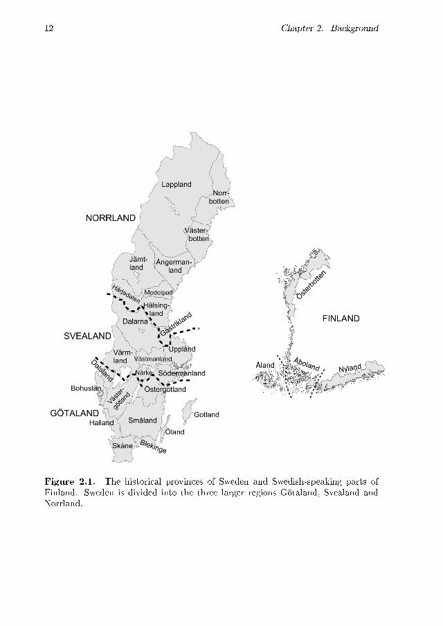
Standard works describing the Swedish dialects are Våra folkmål by Wessén(1969), which was �rst published in 1935, and Svenska dialekter by Pamp (1978).Pamp describes the dialects in each of the historical provinces of Sweden withoutsuggesting any linguistic classi�cation of the dialects, beyond the administrativeprovince borders. Figure 2.1 displays the Swedish provinces. The provinces ofSweden are grouped as belonging to one of the three larger regions Götaland, Svea-land and Norrland. Reference to the province names are used when discussing theresults in the following chapters of this thesis.
Pamp (1978) does not deal with the Swedish dialects in Finland. Descriptions ofthe Finland-Swedish dialects are found in Svenskan i Finland by Ahlbäck (1956) andFrån Pyttis till Nedervetil by Harling-Kranck (1998). Within the Finland-Swedisharea a division according to provinces is usually applied. The provinces with Swedishpopulation in Finland are displayed in Figure 2.1.
Wessén (1969) suggested a linguistic classi�cation of the Swedish dialects into sixgroups. This classi�cation is described more closely in � 2.2.1. Elert (1994) proposeda division of the regional varieties of Standard Swedish that largely resembles theclassi�cation of the traditional rural dialects by Wessén. Elert's classi�cation of theregional varieties of Standard Swedish is described in � 2.2.2.
Recently, data collected in the SweDia project (see � 4.1) have made it possibleto conduct quantitative analyses of modern spoken Swedish. The data was gatheredaround year 2000, and within the project, Swedish dialects have been classi�ed ac-
12 Chapter 2. Background
Figure 2.1. The historical provinces of Sweden and Swedish-speaking parts ofFinland. Sweden is divided into the three larger regions Götaland, Svealand andNorrland.
2.2. Swedish dialect geography 13
cording to some speci�c linguistic features. Since the data for this thesis comprisesvowel data from the SweDia database, an overview of classi�cations made based ondata of other linguistic levels from the same database is given in � 2.2.3. Compar-ing the results of di�erent studies where SweDia data have been used makes sensebecause all the studies involve the same participants recorded at the same pointin time. The studies of variation at di�erent linguistic levels are therefore directlycomparable.
In Swedish dialectology, computational methods have not been very commonlyused (Edlund, forthcoming). In some of the studies described in � 2.2.3, methodsborrowed from the dialectometric research tradition (see � 2.5) have been applied(particularly cluster analysis), and Leinonen (2007) used cluster analysis and multi-dimensional scaling for analyzing vowel pronunciation in Finland-Swedish dialects.However, Swedish dialect geographic works where quantitative methods are usedhave generally focused on some speci�c part of the language system, rather thanaiming at an aggregate analysis, which is what has been the main focus of dialecto-metry. Aggregate dialectometric analyses of the whole Swedish language area do notexist so far. In the dialect atlas of the northern part of Norrland (Hansson, 1995)some summarizing dialectometric maps are included.
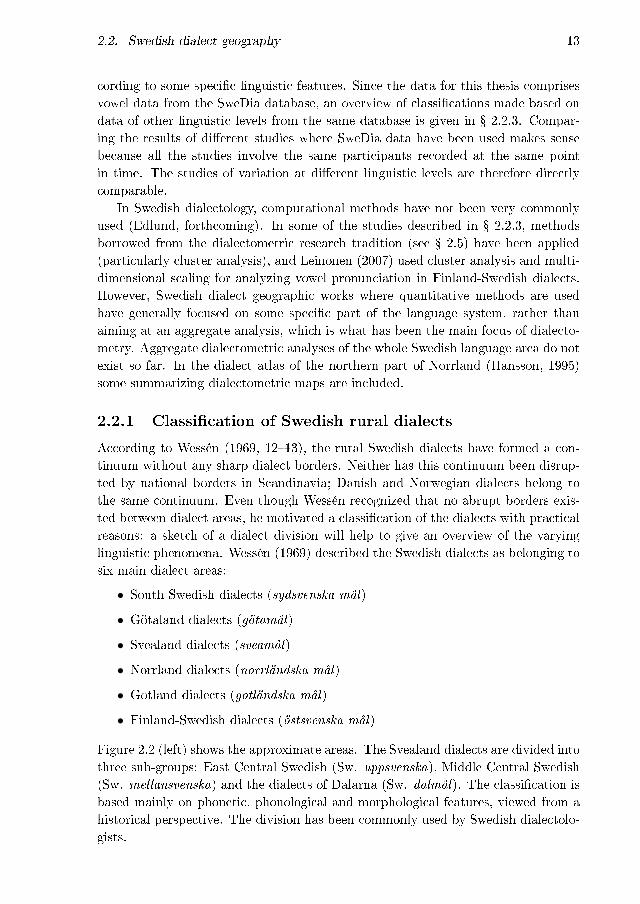
2.2.1 Classi�cation of Swedish rural dialects
According to Wessén (1969, 12�13), the rural Swedish dialects have formed a con-tinuum without any sharp dialect borders. Neither has this continuum been disrup-ted by national borders in Scandinavia; Danish and Norwegian dialects belong tothe same continuum. Even though Wessén recognized that no abrupt borders exis-ted between dialect areas, he motivated a classi�cation of the dialects with practicalreasons: a sketch of a dialect division will help to give an overview of the varyinglinguistic phenomena. Wessén (1969) described the Swedish dialects as belonging tosix main dialect areas:
• South Swedish dialects (sydsvenska mål)
• Götaland dialects (götamål)
• Svealand dialects (sveamål)
• Norrland dialects (norrländska mål)
• Gotland dialects (gotländska mål)
• Finland-Swedish dialects (östsvenska mål)
Figure 2.2 (left) shows the approximate areas. The Svealand dialects are divided intothree sub-groups: East Central Swedish (Sw. uppsvenska), Middle Central Swedish(Sw. mellansvenska) and the dialects of Dalarna (Sw. dalmål). The classi�cation isbased mainly on phonetic, phonological and morphological features, viewed from ahistorical perspective. The division has been commonly used by Swedish dialectolo-gists.

14 Chapter 2. Background
Figure 2.2. The map to the left shows the classi�cation of Swedish rural dialectaccording to Wessén (1969), while the map to the right shows the division of modernspoken Swedish proposed by Elert (1994). The divisions are rather similar.
The South Swedish area includes dialects in the provinces Skåne, Blekinge andsouthern parts of Halland and Småland.
The province Västergötland is the center of the Götaland dialects. Other provincesthat Wessén includes in the Götaland area are Dalsland, northern Småland, north-ern Halland and the south-west of Östergötland. Värmland is also included in theGötaland area, even though it has a special status when it comes to many features.Bohuslän is a transitional area between South Swedish, Götaland and Norwegiandialects. Some Götaland features have spread via Värmland and western parts ofVästmanland to the north.
The center of the Svealand dialects is in Uppland. Uppland together withGästrikland, south Hälsingland, south-east Dalarna, eastern parts of Västmanlandand northern and eastern parts of Södermanland form the East Central Swedish area.Närke and the rest of Södermanland form a transitional area between Svealand andGötaland dialects, and the same is true for Östergötland, north-east Småland andÖland. These dialects are called Middle Central Swedish. The dialects in Dalarna

2.2. Swedish dialect geography 15
are very conservative and divergent and comprise a separate group within the Svea-land dialects.
The Norrland dialects are spoken along the Swedish cost from north Hälsinglandto Norrbotten in the north. Additionally, the dialects in Jämtland can be includedin the Norrland area, even if they share a number of features with Norwegian dia-lects. The dialects in Härjedalen and north-west Dalarna are of a Norwegian type,according to Wessén.
The Swedish dialects in Finland have comprised an East Swedish dialect areatogether with the Swedish dialects in Estonia (spoken along the western coast ofEstonia). However, most of the Swedish population of Estonia �ed to Sweden duringthe Second World War and Estonian-Swedish dialects are almost extinct today. TheFinland-Swedish dialects share many features with the East Central Swedish ones.
The dialects on the island Gotland have preserved many conservative featuresand are very di�erent from mainland-Swedish ones.
2.2.2 Regional varieties of Standard Swedish
The division of the regional varieties of Standard Swedish proposed by Elert (1994)is displayed in Figure 2.2 (right). A comparison of the division of rural Swedishdialects by Wessén (1969) in the same �gure shows many similarities. Elert (1994)proposed three main varieties of Standard Swedish: South Swedish, Central Swedishand Finland-Swedish. Central Swedish was further subdivided resulting in a divisioninto seven groups:
• South Swedish (sydsvenskt talspråk)
• East Central Swedish (östmellansvenskt talspråk)
• West Central Swedish (götiskt-västmellansvenskt talspråk)
• the spoken language of Bergslagen (bergslagstalspråk)
• the spoken standard language of Norrland (norrlandsstandardsvenskt talspråk)
• the spoken language of Gotland (gotlänskt talspråk)
• Finland-Swedish (�nlandssvenskt talspråk)
Elert (1994) based his division mainly on sentence intonation and di�erences in vowelpronunciation. In addition, some varieties are characterized by salient features likethe use of dorsal /r/ in South Swedish or the lack of the word accent distinction inFinland-Swedish. The regional variation in vowel pronunciation in Standard Swedishis discussed in more depth in � 2.3.2.
2.2.3 Typologies based on speci�c features
Based on data from the SweDia database (see � 4.1), Bruce (2004) classi�ed Swedishdialects according to intonational variation. The intonational parameters of themodel were focal accentuation, phrasing, word accentuation and compounding. Seven

16 Chapter 2. Background
distinct dialect regions were identi�ed, largely corresponding to the ones found byElert (1994) (� 2.2.2). Bruce (2004) called the seven intonational types South, West,Central, East, Far East S, Far East N and North. Far East stands for Finland-Swedish dialects, which were divided into two subtypes: Southern (the south coast)and Northern (the west coast).
Schae�er (2005) also used data from the SweDia database. He used cluster ana-lysis for classifying the Swedish dialects based on phonetic variation in quantity.Schae�er found a division into three main types: Southern Swedish (up to Upp-land and Middle Dalarna), Northern Swedish (Norrland and Åland) and Finland-Swedish (mainland Finland-Swedish dialects). The three areas are separated mainlyby consonant length. The Finland-Swedish dialects are characterized by a shorterconsonant than the two other areas in V:C sequences, while the Southern Swedisharea shows a markedly short consonant in VC: sequences. In the Northern areamore preaspiration was found than in the two other areas. The phonetic di�erencesbetween the three types could be connected to the phonological systems of the dia-lects, that is, the presence or absence of VC and V:C: syllables in stressed positions(see � 2.3.3).
Lundberg (2005) used clustering methods for analyzing di�erences in the pronun-ciation of the vowel in the word lat in Swedish dialects analyzed with Mel-frequencycepstral coe�cients (MFCCs, see � 2.4.2). The data of the study comprised oldermale speakers from the SweDia database. The geographic variation in the Swedishvowel a elicited with the word lat was studied and three clusters representing di�er-ent variants of the vowel were found. The study showed that clustering should notbe applied without evaluation. Principal component analysis was used to establishwhich MFCCs were important for identifying the clusters.
2.3 Swedish vowels
The Standard Swedish vowel system is described below in � 2.3.1. As mentionedabove there is no neutral, geographically and socially non-identi�able, StandardSwedish, but a number of regional varieties of Standard Swedish exist. In � 2.3.2the regional di�erences in vowel pronunciation are described.
The vowel systems of Swedish rural dialects di�er from Standard Swedish bothphonetically and phonologically. In � 2.3.3 an overview of some general featuresconcerning a number of Swedish dialects is given.
2.3.1 The Standard Swedish vowel system
Standard Swedish has eighteen vowel phonemes, nine long and nine short ones cor-responding to each other pairwise. Table 2.1 displays these vowels and their Swedishorthographic equivalents. The correspondence between the long and short vowels isnot only an orthographical one, but the correspondence exists in the linguistic com-petence of native speakers and is founded on phonetic similarity as well as morpho-phonological alternations (Linell, 1973, 8).

2.3. Swedish vowels 17
Table 2.1. The Standard Swedishvowel phonemes (Hedelin, 1997).
Swedish Long Shortletter vowel vowel
a /A:/ /a/e /e:/ /efl/i /i:/ /I/o /u:/ /U/u /0:/ /8/y /y:/ /Y/å /o:/ /O/ä /E:/ /Efi/ö /ø:/ /øfl/
The phonemes are displayed with IPA symbols used for Standard Swedish in thepronunciation dictionary Norstedts svenska uttalslexikon (Hedelin, 1997). The pro-nunciation dictionary Svenska språknämndens uttalsordbok (Garlén, 2003) appeareda few years later, but does not use IPA symbols for all vowels, which is the reasonwhy symbols in Norstedts svenska uttalslexikon were chosen to denote the Stand-ard Swedish vowel phonemes and Standard Swedish pronunciation throughout thisthesis.
A few di�erences exist between the two mentioned Swedish pronunciation dic-tionaries. The long a, transcribed [A:] by Hedelin (1997), is transcribed [6:] in themore recent dictionary. Garlén (2003, 31) describes the Swedish long a vowel asa slightly rounded open back vowel. Hence, the actual pronunciation is somethingbetween unrounded [A:] and rounded [6:].
The other vowel for which the two dictionaries have used di�erent IPA symbolsis the short ö. Hedelin (1997) uses [øfl], while Garlén (2003) uses [œ]. Accordingto Garlén (2003) the pronunciation is, thus, more open than according to Hedelin(1997). However, according to both authors the pronunciation of short ö is moreopen than the pronunciation of long ö, which is probably more important than theexact degree of openness of the vowel.
According to Elert (1997) in the Introduction to Norstedts svenska uttalslexikon,the Swedish long o is somewhat more open than the cardinal vowel [u]. Thereforethe phonetic symbol [Ñ:] is used in Norstedts svenska uttalslexikon. The symbol [Ñ]denotes a semi-high back rounded vowel, but was marked as obsolete by IPA in1989 and is not used in the newest version of the International Phonetic Alphabet.Throughout this thesis [u:] is therefore used for the Standard Swedish long o.
The pronunciation of long u in Standard Swedish is actually more fronted thanthe symbol [0:] suggests. According to Elert (1997) a more precise phonetic symbolwould be [0ff:].
In addition to the eighteen phonemes, more open allophones of ä and ö are usedwhen these vowels are followed by /r/ (which is equal to [r] or a retro�ex consonantresulting from the consonant combinations rd, rl, rn, rs and rt):

18 Chapter 2. Background
• /E:/ → [æ:]
• /Efi/ → [æ]
• /ø:/ → [œ:]
• /øfl/ → [œ]
In an acoustic analysis of Swedish long vowels, Eklund & Traunmüller (1997) showedthat only /A:/ and [æ:] are plain monophthongs.3 Especially the mid vowels, /o:/,/ø:/ and /e:/, showed substantial diphthongization. These vowels are pronouncedas opening diphthongs; F1 increases in the course of the vowels, and F2 decreasesin the front vowels, /ø:/ and /e:/, and increases in the back vowel /o:/. The closevowels (/i:/, /y:/, /0:/ and /u:/) showed smaller formant movements than the midvowels. The close vowels �rst become even more close and only at the very end morecentralized. The subjects (six male and six female in the age range 20�58) were fromthe greater Stockholm area.
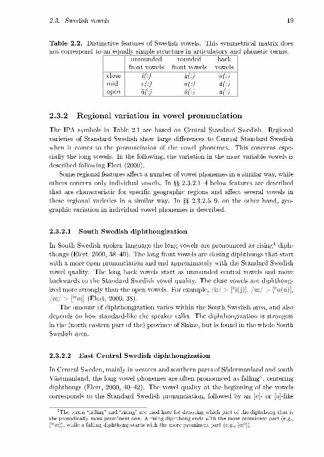
Describing the Swedish vowels with distinctive features has turned out to be com-plicated. A simple matrix, which in addition to the length distinction includes threedegrees of openness, a front�back distinction, and a roundness distinction for frontvowels, can be set up (Table 2.2). The problem is that this simple matrix does notcorrespond to �an equally simple structure of articulatory or acoustic facts� (Fant,1971, 259). Linell (1973) summarizes the problems involved in a phonological de-scription of Swedish vowels and reviews the most common solutions suggested. Thebiggest problem is the phoneme /0:/ and its short counterpart /8/. In articulatoryterms /0:/ is a close or near-close and extremely rounded front vowel, while /8/ isa mid vowel. The articulatory and perceptual distance between the long and shortvariant is hence large. In the di�erent suggested phonological interpretations, theposition of /0:/ and /8/ has varied in both the height dimension and on the front�back scale. Linell (1973) proposes that /0:/ should be treated as a central vowelphonologically. Other researchers treat /0:/ as a front vowel and use three degreesof roundness (unrounded, out-rounded, in-rounded) for distinguishing /0:/ from /i:/and /y:/ (Traunmüller & Öhrström, 2007) or from /e:/ and /ø:/ (Malmberg, 1956).
A problem with the simple solution in Table 2.2 is that it pushes ö into a moreopen position than articulatory and acoustic data suggest, and that u is not groupedwith the other close vowels, with which it shares important features (see, for example,� 2.3.2.4). Other problems with phonological descriptions of the Swedish vowels havebeen how to �t in the pre-/r/ variants of ä and ö, and that the long a is a backvowel but it's shorter counterpart a central vowel. Linell (1973, 12) points out that,interestingly enough, the vowels that present a problem for the phonological descrip-tion of the Standard Swedish vowels are the same that seem to show considerablevariation across Swedish dialects.
3/E:/ was not included, because the subjects were asked to pronounce the Swedish letter names.The name of the letter ä is pronounced [æ:], while all other letters are pronounced as the corres-ponding long vowels in Table 2.1.
2.3. Swedish vowels 19
Table 2.2. Distinctive features of Swedish vowels. This symmetrical matrix doesnot correspond to an equally simple structure in articulatory and phonetic terms.
unrounded rounded backfront vowels front vowels vowels
close i(:) y(:) o(:)mid e(:) u(:) å(:)open ä(:) ö(:) a(:)
2.3.2 Regional variation in vowel pronunciation
The IPA symbols in Table 2.1 are based on Central Standard Swedish. Regionalvarieties of Standard Swedish show large di�erences to Central Standard Swedishwhen it comes to the pronunciation of the vowel phonemes. This concerns espe-cially the long vowels. In the following, the variation in the most variable vowels isdescribed following Elert (2000).
Some regional features a�ect a number of vowel phonemes in a similar way, whileothers concern only individual vowels. In �� 2.3.2.1�4 below features are describedthat are characteristic for speci�c geographic regions and a�ect several vowels inthese regional varieties in a similar way. In �� 2.3.2.5�9, on the other hand, geo-graphic variation in individual vowel phonemes is described.
2.3.2.1 South Swedish diphthongization
In South Swedish spoken language the long vowels are pronounced as rising4 diph-thongs (Elert, 2000, 38�40). The long front vowels are closing diphthongs that startwith a more open pronunciation and end approximately with the Standard Swedishvowel quality. The long back vowels start as unrounded central vowels and movebackwards to the Standard Swedish vowel quality. The close vowels are diphthong-ized more strongly than the open vowels. For example, /i:/ > [ei(j)], /u:/ > [eU(u)],/ø:/ > [œø:] (Elert, 2000, 38).
The amount of diphthongization varies within the South Swedish area, and alsodepends on how standard-like the speaker talks. The diphthongization is strongestin the (north-eastern part of the) province of Skåne, but is found in the whole SouthSwedish area.
2.3.2.2 East Central Swedish diphthongization
In Central Sweden, mainly in western and southern parts of Södermanland and southVästmanland, the long vowel phonemes are often pronounced as falling4, centeringdiphthongs (Elert, 2000, 40�42). The vowel quality at the beginning of the vowelscorresponds to the Standard Swedish pronunciation, followed by an [e]- or [@]-like
4The terms �falling� and �rising� are used here for denoting which part of the diphthong that isthe prosodically most prominent one. A rising diphthong ends with the more prominent part (e.g.,[œø:]), while a falling diphthong starts with the more prominent part (e.g., [ø:@]).

20 Chapter 2. Background
quality. Sometimes laryngalization occurs between these two elements. Examples,/i:/ > [i:(j)@], /u:/ > [u:(B)@], /ø:/ > [ø:@] (Elert, 2000, 40).
This diphthongization has been shown to be prosodically conditioned (Bleckert,1987). It is strongest in stressed long vowels and at the end of sentences. It is arather new feature that was �rst attested in some Central Swedish towns at thebeginning of the 20th century. Strong diphthongization is not commonly acceptedas Standard Swedish (Elert, 2000, 42).
2.3.2.3 Gotlandic diphthongization
The dialects on Gotland are characterized by both archaic diphthongs and secondarydiphthongs (see � 2.3.3). Some of these diphthongs are only part of the rural dialects,but also in standard-like Swedish spoken on Gotland some of the long vowels arediphthongized (Elert, 2000, 42�43). The diphthongization concerns mainly the midvowels, but the pattern is not as clear as in South Swedish and East Central Swedishdiphthongization. Some of the diphthongs are falling, while others are rising; someare closing, while others are centering: /e:/ > [e:I], /E:/ > [eE:], /0:/ > [E0], /ø:/ >[ø:Y], /u:/ > [ou:], /o:/ > [o:E] (/i:/, /y:/ and /a:/ are monophthongs) (Elert, 2000,42).
2.3.2.4 Semi-vowel/fricative ending in long close vowels
The long close vowels are followed by a consonantal segment in large parts of Sweden:/i:/ > [ij], /y:/ > [y4], /0:/ > [0B] and /u:/ > [uB] (Elert, 2000, 43�44). Theconsonantal ending is most prominent in word �nal position or before another vowel.
This feature is common in the spoken language in the Central Swedish area. InSouth Swedish it is less prominent and in Norrland and Finland it hardly exists.
2.3.2.5 Damped i and y
The Swedish �damped� i and y are common in the East Central Swedish area (Elert,2000, 44�45). These variants of the Swedish /i:/ and /y:/ are pronounced with amarkedly low F2, so that they sound more retracted than in Standard Swedish,closer to [1] and [0] (Björsten & Engstrand, 1999). They are also co-articulatedwith a fricative consonant, which gives a characteristic buzzing sound, and, hence,are often transcribed as [iz] and [yz] (which is not entirely appropriate because thebuzzing is present in a larger part of the vowel segment and not only at the end).
The damped pronunciation of i and y has a special distribution. It can be foundin some scattered rural dialects, but also in the spoken language in Stockholm andGöteborg. In the areas where the damped pronunciation is part of the rural dialectspeakers tend to leave out this feature when they want to speak more standard-like,while in the cities, Stockholm and Göteborg, the damped pronunciation is consideredposh (Elert, 2000, 45).

2.3. Swedish vowels 21
2.3.2.6 Long and short e and ä
In large parts of the language area the short vowels /efl/ and /Efi/ are two separatephonemes (Elert, 2000, 46). However, in East Central Swedish and in the varietieson Gotland and in Finland the two phonemes have merged. Johansson (1982, 94)found that /efl/ and /Efi/ were maintained as two separate phonemes by most speakersin a number of towns in Norrland. For young female speakers, however, she founda perceptual merger of these two phonemes. The merger seems to be more commonamong younger speakers than among older speakers today, and might be regardedas unmarked standard pronunciation nowadays.
In a smaller geographic area the corresponding long vowels /e:/ and /E:/ havemerged, too, both being pronounced [e:]. However, it is not a complete merger, butbefore /r/ the two phonemes are kept apart. So there is a distinction between, forexample, lera [le:ra] `clay' and lära [læ:ra] `learn', but not between leka [le:ka] `play'and läka [le:ka] `heal'. The merger has been part of the traditional dialects in thesurroundings of Stockholm and is also found in Finland. Contrary to the mergerof the short e and ä the merger of the corresponding long vowels is not acceptedin Standard Swedish pronunciation and there seems to be a reversal of the mergergoing on (Elert, 2000, 46).
In a study of the language of teenagers in Stockholm, Kotsinas (1994) foundthree variants of /E:/: [e:], [E:] and [æ:]. The pronunciation [e:] was more frequentin the lower social class than in the higher social class, while [æ:] was more frequentin the higher social class. The open pronunciation [æ:] could be interpreted as areaction against �uncultivated� Stockholm-speech.
2.3.2.7 Long and short u and ö
The pronunciation of /ø:/ shows considerable variation (Elert, 2000, 47�48). InEast Central Sweden a more open pronunciation, [œ:], has become popular amongyounger speakers. Kotsinas (1994) found that the open pronunciation was the mostcommon one among Stockholm teenagers in all social groups. According to Elert(2000, 47), the more open pronunciation is common across generations in some partsof Sweden, for example Östergötland, Västergötland and Värmland.
The vowel written with the letter u in Swedish had the pronunciation [u(:)] inthe 12th and 13th centuries when the Latin alphabet was introduced in Scandinavia.After that the vowel has been fronted leading to [0:/0ff:] and [8] in modern Swedish.This process has not had the same speed across the entire language area. Some ruraldialects and regional standard varieties have a more central or back pronunciation ofu than Standard Swedish, for example, Finland-Swedish and varieties in south-westSkåne, Dalarna and north Västmanland (Elert, 2000, 49).
The short vowels /8/ and /øfl/ are merged in the speech of many speakers in EastCentral Sweden (Elert, 2000, 48). Wenner (2010) showed that younger speakers inUppland have a shorter acoustic distance between /8/ and /øfl/ than older speakers,which suggests an ongoing change. The merger is more common when an /r/ ispreceding or following the vowel than in other contexts.

22 Chapter 2. Background
2.3.2.8 The open allophones of ä and ö before r
As mentioned above, the ä and ö vowels have more open allophones that are usedonly before /r/. However, the degree of openness of these allophones varies. Theopen allophones are pronounced most open along the east coast and in Finland(Elert, 2000, 48�49). In the west they are more close and in some places there areno allophones, so that the vowels have the same pronunciation in all positions.
In a study of attitudes towards Swedish dialects by Bolfek Radovani (2000) notonly the pronunciation [e:] of /E:/ in Uppland, but also the extremely open [æ:]before /r/ were seen as stigmatized variants of which the dialect speakers themselveswere highly aware.
2.3.2.9 Long and short a
The long a vowel is a slightly rounded open back vowel in Standard Swedish. Amongsome speakers in Stockholm and Göteborg the vowel is even more rounded and close,almost [O:] (Elert, 2000, 50). In Finland the vowel is generally more fronted andunrounded: [a:].
In a few areas, the short vowel /a/ has a pronunciation closer to [æ]. Elert (2000,51) mentions east Småland and Eskilstuna.
2.3.3 Vowel systems of the Swedish dialects
The rural dialects in the Swedish language area di�er from Standard Swedish atpractically all linguistic levels (segmental, prosody, phonology, morphology, lexicon,semantics, syntax). The vowel systems of the dialects di�er from Standard Swedishnot only in the pronunciation of the vowel phonemes, but also in the number ofphonemes.
The di�erences in the vowel systems of the Swedish dialects in comparison toStandard Swedish are partly due to archaic features and partly due to innovations.Archaic features are, for example, the preservation of the Proto-Nordic diphthongs/ai/, /au/ and /eu/. These diphthongs were monophthongized in large parts of east-ern Scandinavia around 900�1100 and partly merged with original monophthongs.In Standard Swedish these original diphthongs have been replaced by long vowels.The monophthongization spread from the south and never reached some peripheraldialect areas. Dialects on Gotland, in parts of Finland and in parts of Norrland werenever a�ected and have preserved the original diphthongs (Pettersson, 2005).
Another type of diphthongs in the Swedish dialects are the so-called secondarydiphthongs. These have developed from original monophthongs which have beendiphthongized in some dialects. Secondary diphthongs are characteristic for thesouthern provinces of Sweden, but are also found on Gotland and in some Finland-Swedish dialects.
Another archaic feature is the preservation of the Proto-Nordic long a. During the13th and 14th centuries the pronunciation of this phoneme became more close andback resulting in the å [o:] in modern Swedish. This change, too, never reached some

2.4. Acoustic analysis of vowels 23
peripheral areas (for example Gotland), which preserved a more open pronunciation[a:]/[A:].
The Swedish quantity shift, around 1200, a�ected the vowel systems of the dia-lects in di�erent ways. In Proto-Nordic four types of syllables could occur in stressedpositions: VC, V:C, VC: and V:C:. The quantity shift resulted in the loss of VCand V:C: sequences in stressed syllables. In modern Standard Swedish and mostdialects all stressed syllables have either a long vowel followed by a short consonant(V:C) or a short vowel followed by a long consonant or a consonant cluster (VC: orVCC). During the quantity shift, the new system was reached in di�erent ways bydi�erent dialects. In some dialects the vowel in VC sequences was lengthened, whilein other dialects the consonant was lengthened. Also the quality of the short vowelswas a�ected di�erently in di�erent dialects (Pettersson, 2005, 224�227). Some dia-lects were not a�ected at all, or only partly, by the quantity shift (mainly dialectsin Norrland and Finland).
Even though there is a long tradition of dialect research in Sweden and Finland,the phoneme systems of Swedish dialects as spoken nowadays are largely unknown.Structural descriptions of the vowel systems of dialects are rare, and because ofthe large changes that the dialects have gone through since the middle of the 20thcentury older descriptions of the phoneme systems are not necessarily valid anymore.Many dialects have not been the subject of recent studies, and even for dialects thathave recently been studied, describing the phoneme system is not always easy. In aphonological analysis of the Swedish dialects of the province Österbotten in Finland,known for well-preserved rural dialects, Wiik (2002) concluded that especially thelong vowel systems are di�cult to describe. The traditional rural dialects have morelong vowels than short vowels, mainly due to diphthongs among the long vowels.However, because of dialect leveling the long vowel systems are unstable. Thereare, for example, tendencies to monophthongize diphthongs, and in words borrowedfrom Standard Swedish phonemes that have not originally been part of the ruraldialect, are used. The study by Wiik (2002) included the dialects of 30 parishes inÖsterbotten. Only a few of these dialects showed identical long vowel systems. Thenumber of long vowel phonemes varied between ten and sixteen, while the numberof short vowel phonemes was less variable (between seven and nine short vowelphonemes).
2.4 Acoustic analysis of vowels
When studying phonetic di�erences between languages or language varieties we canchoose to work either with phonetically transcribed data or with acoustic analysisof speech samples. A disadvantages of phonetic transcription is that it requires alarge amount of work and still is not a very exact method. Linguistic experience willin�uence the decisions even of highly trained transcribers (Dioubina & P�tzinger,2002), and transcribers do not even always agree with themselves when transcribingthe same utterance multiple times (P�tzinger, 2003).

24 Chapter 2. Background
Numerous e�orts have been made to assess phonetic quality of speech segmentsdirectly from the acoustic signal. The most common way of measuring vowel qualityacoustically are formant measurements, explained in � 2.4.1. Another approach areso-called whole-spectrum methods. Di�erent whole-spectrum methods are discussedin � 2.4.2.
Analyzing vowel quality acoustically is a more objective method than using tran-scriptions, but does not come without its own problems. The acoustic signal in-cludes information that is not linguistically meaningful, but has to do with anatom-ical/physiological di�erences between speakers (� 2.4.3). Transcribers are very goodat ignoring spectral di�erences that are due to speaker-speci�c variation and reportthe actual linguistic di�erences that they perceive. But when working with acousticspeech data, normalizing for the non-linguistic speaker-dependent variation has al-ways been problematic. Di�erent approaches to speaker normalization are discussedin � 2.4.4.
2.4.1 Measuring formants
Since the work of Peterson & Barney (1952) formant measurements have been theclassical way of measuring vowel quality. The two �rst formants (i.e. the lowestresonance frequencies of the vocal tract during pronunciation) are the most distinct-ive acoustic parameters that determine vowel quality. These correspond relativelywell to the articulatory vowel features height and advancement. This can be seen inthe spectrograms in Figure 2.3. The horizontal axis shows time, while the verticalaxis shows frequency. The intensity of the speech signal at di�erent frequencies ata given time is expressed by the darkness of the shading. The formants show upas darker bands in the spectrogram. [i] and [u] which are both close vowels have alow �rst formant (F1, the lowest formant), while the open vowels [æ] and [a] have ahigher F1. The front vowel [i] has a high frequency for F2, while the back vowel [u]has a very low F2. The F2 values for [æ] and [a] are in between these two extremes.
A two-dimensional graph, Figure 2.4, where the two dimensions represent tongueadvancement and height has been used by phoneticians to display the main para-meters of vowel production. Joos (1948) showed that vowels plotted in an acousticplane, where F2 is represented on the horizontal axis and F1 on the vertical axiswith the origin in the upper right corner, leads to a relatively similar con�gurationas the articulatory graph. This parallel between the articulatory and acoustic planesis indicated with the arrows in Figure 2.4. However, the correspondence betweenformants and vowel height and advancement is not perfect. Rosner & Pickering(1994, 46�48) show that altering the three articulatory parameters constriction size,constriction location and mouth opening in vowels does not have any one-to-onecorrespondence with formants, but both the F1 and the F2 values are in�uenced bythe change in any of the articulatory parameters.
The third formant also plays a role in vowel categorization, but this is less wellunderstood than F1 and F2. The importance of F3 seems to vary across languages,and for some languages the �rst two formants are enough for listeners to identify all

2.4. Acoustic analysis of vowels 25
Figure 2.3. Vowel spectrograms of [i], [æ], [a] and [u]. The dashed lines mark theapproximate positions of the formants.
Figure 2.4. Vowel quadrilateral (vowel chart of the International Phonetic As-sociation) with formant a�liation. F1 and F2 (Hz) with values of a typical malevoice.

26 Chapter 2. Background
vowels (for a discussion of this see Adank, 2003, 38�39). However, phoneticians warnagainst using only F1 and F2 in a routine manner since some valuable data presentin third formant might get lost. Fujimura (1967) found that for the identi�cation ofSwedish front rounded vowels F3 seems to be important.
In Figure 2.3 the three �rst formants can be most clearly distinguished in thecase of [æ]. The vowel [i] has a large distance between F1 and F2, while F2 and F3are so close to each other that they are hard to distinguish. In the cases of [a] and[u] F1 and F2 are very close to each other.
Linear predictive coding is the most commonly used computational method forestimating formant frequencies from a speech signal (Rosner & Pickering, 1994, 8�11). A problem with algorithms for automatically determining formant frequencies ina spectrum is that they always give some false measurements. Formants very close toeach other (like F1 and F2 in [u]) sometimes cannot be separated by the algorithms,and on the other hand the algorithms sometimes �nd false formants in the gapbetween formants if two adjacent formants have a large distance (like F1 and F2 in[i]). In a study of Swedish vowels by Eklund & Traunmüller (1997), where formantswere �rst measured automatically and subsequently checked manually, correctionshad to be made for approximately a quarter of the vowel segments. Likewise, Adank,Van Hout, & Smits (2004) report that the automatic formant measurements of 20�25% of the vowels in a Dutch study had to be corrected manually.
Formant measurement has been used for measuring vowel quality in a numberof large-scale studies of regiolects and sociolects. Labov, Ash, & Boberg (2005)described regional varieties of North American English by measuring the �rst twoformants of on average 300 vowel tokens of 439 speakers. Adank, Van Hout, & Van deVelde (2007) investigated regional di�erences in vowel pronunciation in StandardDutch based on measurements of duration and formant frequencies of 15 vowelsof 160 Dutch and Flemish speakers. Clopper & Paolillo (2006) analyzed formantfrequencies and duration of 14 American English vowels as produced by 48 speakersfrom six dialect regions. However, the need for manual correction of the data makesformant measurements a very time-consuming method when working with data setsincluding a large number of speakers.
2.4.2 Whole-spectrum methods
Besides formant-based approaches to measuring vowel quality whole-spectrum meth-ods are also used. These are sometimes preferred since they include more acousticinformation than formant frequencies. Moreover, whole-spectrum methods can gen-erally be more reliably automated than formant analysis, which makes them moresuitable for fast analysis of large amounts of data.
In the 1960s, Dutch researchers introduced principal component analysis (PCA)of band-pass-�ltered5 spectra as a method for identifying vowels acoustically (Plomp,
5Applying an acoustic �lter means that sound energy above and/or below a given frequency in

2.4. Acoustic analysis of vowels 27
Pols, & Van de Geer, 1967). Vowel spectra were band-pass �ltered with 13 -octave
�lters, roughly corresponding to the ear's critical bandwidth. The vowel spectrawere �ltered up to 10,000 Hz, which, after combining the lowest �lters in order toreduce the e�ect of fundamental frequency and for even better correspondence withthe critical bandwidth, resulted in each vowel being described by the sound-pressurelevels in decibels in 18 pass bands. PCA was used to �nd the linear combina-tions of the pass bands in the �lter bank representation that would explain mostof the variance in the data. The two �rst principal components (PCs) turned outto explain most of the variance (68.4%), while extracting up to four PCs signi�c-antly improved the amount of explained variance (84.1%). The PCs were shownto correlate highly with perceptual dimensions used by listeners to identify vowels(Pols, Van der Kamp, & Plomp, 1969). The method was mainly seen to be a use-ful application within automatic speech recognition. An advantage of a �lter bankrepresentation over measuring formants is that using band-pass �ltering and PCA ismuch faster than formant analysis and does not require manual correction. The two�rst PCs correspond well with the two �rst formants. Correlating average formantsvalues of twelve vowels pronounced by 50 male speakers showed very high correlation(r = 0.989 and r = 0.993) with the two �rst PCs after an optimal rotation of thePC plane (Pols, Tromp, & Plomp, 1973). However, correlating formants with thePC values of the individual speakers showed signi�cantly less correspondence. In anautomatic recognition task vowels were identi�ed about equally well using formantsand PCs (Pols et al., 1973).
Van Nierop, Pols, & Plomp (1973) compared the results of a PCA on band-pass�ltered spectra of twelve Dutch vowels by 25 female speakers to the earlier resultsby Klein, Plomp, & Pols (1970) and Pols et al. (1973) based on 50 male speakerspronouncing the same vowels. The eigenvectors of the two �rst components wererather similar for the female and male data, but the peaks in the curves of the femaleanalysis occurred about 1
3 -octave higher than the corresponding curves for the maledata. The extracted components were not identical for the female and male data,but a small rotation of one of the two con�gurations showed that there was almosta complete convergence of the two solutions after rotation.
Jacobi (2009) applied PCA to band-pass �ltered spectra in a study of variationin Dutch diphthongs and long vowels (/Ei/, /Au/, /œy/, /o:/ and /e:/) among 70speakers (35 female and 35 male). Her aim was to �nd out if the sub-phonemicvariation in these vowels could be related to socio-economic status and the age ofthe speakers. Band-pass �ltering was chosen over formant analysis, since it can befully automated without the need for manual correction of errors and yet, throughhigh correlation with formants, o�ers interpretability in terms of articulatory andperceptual attributes. However, applying the method introduced by Plomp et al.(1967) to a variational linguistic study presented some challenges. The experimentsof the Dutch researchers in the 1960s and 1970s were done in controlled environments.
a sound spectrum is �ltered away. The part of the spectrum remaining is called a pass band. Aband-pass �lter can be characterized by its center frequency and bandwidth. See Johnson (2003,14�17).

28 Chapter 2. Background
Jacobi's data, on the other hand, consisted of spontaneous speech from the CorpusGesproken Nederlands (= Corpus of Spoken Dutch) in extremely varying recordingsituations. Plotting the speakers /a/�/i/�/u/ vowel triangles in the PC2/PC1 planeshowed a remarkable variability between speakers in the positioning of the triangles.The di�erences could be traced back to the signal-to-noise ratios in the recordings,which varied from interviews in silent environments to private conversations andbroadcast recordings with music in the background. It turned out that the lowerthe signal-to-noise ratio (that is, the more noise), the smaller the measured vowelspace in the PC plane and the higher the PC values. Vowels produced by menand women were analyzed together in the PCA. Some signi�cant di�erences in thePC values between the sexes were found, but these were small compared to thedi�erences depending on the varying recording situations. In order to normalize forthe di�erences in position and size of the vowel spaces of di�erent speakers, relativePC values were used: the positions of all vowels in the PC plane were related tothe speaker's point vowels /i/ and /a/.6 In order to enhance the interpretabilityof the PCA solution Jacobi used only point vowels to build up the PCA. Whenan equal number of all point vowels are used in the analysis phase of the PCA, allarticulatory-acoustic dimensions are represented equally and all possible di�erencesin vowel quality are accounted for. The results can then be used to represent allother vowels within the vowel space.
For the band-pass �ltering, Jacobi used Bark �lters instead of 13 -octave �lters.
The Bark scale is a psycho-acoustical scale corresponding to the critical bandwidthof human hearing, which means that a representation in Bark �lters should corres-pond to how humans perceive vowel sounds. The Bark scale is roughly linear up to1000 Hz and roughly logarithmic at higher frequencies. Jacobi found high correla-tions between PCs and formants (see � 5.2.1) and concluded: �pc1 and pc2 of a PCAon bark�ltered /a/, /i/, /u/ yielded comparable results to F1Bark and F2Bark, andare thus easily interpretable in terms of articulation� (Jacobi, 2009, 42).
In automatic speech recognition Mel frequency cepstral coe�cients (MFCCs) arewidely used today for identifying speech sounds. Like the Bark scale, the Mel scaleis an auditory scale (a doubling of Mels corresponds to the doubling of perceivedpitch). MFCCs are obtained by applying discrete cosine transformation to Mel-scaled bandpass �lters (Harrington, 2010). In a study exploring cluster analysis asa method for classifying dialects Lundberg (2005) applied MFCCs to vowel datafrom 285 subjects from 95 sites in the Swedish language area (see also � 2.2.3). Areduction of twelve MFCCs to two dimensions by multidimensional scaling showeda con�guration similar to the IPA vowel quadrilateral (Lundberg, 2005, 26).
For the present study PCA on Bark �ltered vowel spectra was chosen for ana-lyzing vowel segments acoustically. The main reason for choosing a whole-spectrummethod instead of measuring formants is that the whole-spectrum methods havebeen shown to be more reliably automatable than formant measurements. Choosinga method which does not need manual correction was important, because the data
6Because /u/ was the most sensitive point vowel to the signal-to-noise ratio only /i/ and /a/were used for calculating the relative positions.

2.4. Acoustic analysis of vowels 29
for the present study includes nearly 1,200 speakers (see Chapter 4). MFCCs couldhave been chosen instead of Bark �lters and PCA, and might yield similar results.
The method and its application to the present data set is described more closelyin Chapter 5. In addition to band-pass �ltering, formant analysis was applied to asmaller subset of the data in order to validate the method and to �nd the optimalPCA con�guration (see � 5.2).
2.4.3 Speaker-dependent variation in vowels
A challenge for all acoustic methods is the speaker-dependent di�erences in speechsounds due to the di�erent size and shape of the vocal tract of speakers. Two vowelsuttered by two di�erent speakers can have very similar formant frequencies whilethey are perceived as belonging to di�erent phonemes by listeners of the languages.And, conversely, two vowels sounding the same to listeners might di�er in formantfrequencies. Generally a smaller vocal tract generates higher formant frequencies.This is why children have higher formant frequencies than adults and women gen-erally higher than men (Peterson & Barney, 1952). But also within age and gendergroups individuals show a lot of variation.
Figure 2.5 shows an example of the inter-speaker variability in formant meas-urements. In the graphs the formant frequencies in Bark of ten Swedish long vow-els produced by three adult speakers, two female (yw_1 and yw_3) and one male(ym_2), are plotted. The speakers all speak the same dialect, the dialect of Malung.The data come from the data set discussed in � 5.2 below. It is evident that thevowel spaces vary both in size and position in the F2/F1 plane (scales are reversedin order to resemble the articulatory vowel quadrilateral). If looking at the absoluteformant frequencies in Bark, the [u:] in sot of speaker yw_1 is closest to the [o:]in lås of ym_3. The [æ:] (lär) of the male speaker (ym_2) is closest to the [œ:](dör) of the two female speakers. However, the relative positions of the vowels in allspeakers' vowel spaces resemble each other a lot.
Inter-speaker di�erences, like the ones present in formant measurements, areusually found also when using whole-spectrum methods for vowel analysis.
The mechanisms behind the speaker normalization that listeners perform arenot fully understood. The problem has been viewed both from a vowel-extrinsic andfrom a vowel-intrinsic perspective. Extrinsic adaptation means that listeners adaptto every speaker's vowel system as a whole, while intrinsic adaptation means thatthe information needed for normalization is included in each segment itself. Intrinsicfactors have been sought in distances between fundamental frequency and higherformants. Fundamental frequency (F0) seems to be an important cue for identifyingvowels in mixed speaker conditions as shown in experiments by Nusbaum & Morin(1992), Eklund & Traunmüller (1997) and Halberstam & Raphael (2004).

30 Chapter 2. Background
Figure 2.5. The vowel spaces of three speakers of the same dialect (Malung). Tendi�erent long vowels are plotted in the F1�F2 plane. The words used for elicitingthe vowels are displayed: dis [i:], dör [œ:], lat [A:], leta [e:], lus [0:], lås [o:], lär [æ:],sot [u:], söt [ø:], typ [y:].

2.4. Acoustic analysis of vowels 31
Table 2.3. Division of formant-based speaker normalization procedures into fourgroups. The division was introduced by Adank (2003).
Formant-intrinsic Formant-extrinsic
Vowel-intrinsicscale transformations Syrdal & Gopal (1986)(e.g. Bark, Mel)
Vowel-extrinsicGerstman (1968) Nordström & Lindblom (1975)Lobanov (1971) Miller (1989)Neary (1977)
2.4.4 Speaker normalization
A wide range of di�erent normalization procedures for vowels have been suggested indi�erent studies. The choice of a normalization procedure depends crucially on theaim of the normalization. For example, in automatic speech recognition systems theaim is to remove all other kinds of variation but the phonemic. For sociolinguisticand dialectological research on the other hand we are interested in also maintainingsub-phonemic variation. The aim of speaker normalization procedures has beendescribed by Disner (1980) as follows: �they should maximally reduce the variancewithin each group of vowels presumed to represent the same target when spoken bydi�erent speakers, while maintaining the separation between such groups of vowelspresumed to represent di�erent targets�.
2.4.4.1 Formant-based normalization procedures
Adank (2003) divided formant-based normalization procedures into formant-intrinsicand formant-extrinsic, as well as vowel-intrinsic and vowel-extrinsic (Table 2.3).Vowel-intrinsic means that the normalization can be done using information presentin a single vowel token, while vowel-extrinsic means that the whole vowel space ofa speaker, or at least the point vowels, are taken into account when performingthe normalization. Formant-intrinsic means that each formant can be normalizedwithout knowledge of higher or lower formants (including F0). Formant-extrinsicmethods use information across formants, for example, relative distances betweenformants (including F0).
A vowel�intrinsic/formant�intrinsic method is basically a transformation of form-ant values according to some scale. The Hertz scale that is used for measuringfrequencies is a linear scale. Bark and Mel are examples of auditory scales, whichcorrespond better to human perception, which is roughly linear up to 1000 Hz androughly logarithmic at higher frequencies. Transforming the measured Hertz valuesto an auditory scale improves the correspondence between acoustic measures andperception.
A vowel-intrinsic/formant-extrinsic procedure was used by Syrdal & Gopal (1986).In this method the data was transformed by measuring the distances in Bark betweenadjacent formants.
Several methods use information across vowel categories for speaker-normaliza-tion (vowel-extrinsic methods). Gerstman (1968) introduced a method for normaliz-

32 Chapter 2. Background
ing on the basis of the highest and lowest F1 and F2 values of each speaker. Lobanov(1971) did a z -transformation of the F1 and F2 values of every speaker. Neary (1977)applied a log transformation to the Hertz frequencies and centered the formant val-ues of every speaker. In Neary's approach the center of every speaker's vowel spaceswas moved to zero, but varying sizes of the vowel spaces of di�erent speakers werenot normalized for. Labov (1994) has used Neary's log mean transformation in hissociolinguistic studies.
A problem with the vowel-extrinsic methods is that they assume that either theaverage values or the extreme values of all speakers are linguistically stable. Theapproaches of Lobanov (1971) and Neary (1977) imply that all speakers use the samephoneme system and that data of all vowel categories are present for all speakers.Otherwise the average values of di�erent speakers would not be comparable. In theprocedure by Gerstman (1968) a reliable transformation is possible only if the vowelphonemes representing the highest and lowest F1 and F2 values are linguisticallystable without sub-phonemic variation.
The vowel-extrinsic/formant-extrinsic normalization procedures use informationacross vowel tokens and across formants. In addition to being vowel-extrinsic/formant-extrinsic the normalization procedure by Nordström & Lindblom (1975) is speaker-extrinsic. In their study Nordström & Lindblom (1975) started by estimating theaverage length of vocal tracts of men and women by calculating average F3 values ofopen vowels within each sex group. Because the length of the vocal tract correlateshighly with formant frequencies, a scale factor based on the ratios between averagemale and female vocal tract lengths (as estimated by F3) could be used for trans-forming the formant frequencies. This procedure does not remove speaker-dependentdi�erences within the two sex groups, but it normalizes for the systematic di�erencesbetween male and female voices.
The normalization procedure of Miller (1989) is based on distances between form-ants, hence, formant-extrinsic. Furthermore a speaker-speci�c anchor point basedon average F0 values is used, which makes it vowel-extrinsic.
2.4.4.2 Normalization in whole-spectrum approaches
A centering of data, corresponding to the procedure of Neary (1977), was used onbandpass-�ltered vowel data by Pols et al. (1973). Jacobi (2009) applied centeringto principal components of bandpass-�ltered data, but decided on using anothermethod for speaker normalization. The point vowels /i/ and /a/ were consideredstable point vowels in the Dutch data in Jacobi's study. Hence, positions relativeto each speaker's /i/ and /a/ were calculated for all vowels, which accounted fordi�erences in the size and position of the vowel spaces of di�erent speakers.
Both the method of Pols et al. (1973) and the one of Jacobi (2009) are vowel-extrinsic and, therefore, depend either on identical phoneme systems or stable pointvowels in the data.

2.4. Acoustic analysis of vowels 33
2.4.4.3 Evaluations of normalization procedures
When comparing di�erent vowel normalization procedures Disner (1980) found thatNeary's log-mean procedure was best at reducing scatter within languages. But acrucial result from her study was that most of the procedures tested performed quitepoorly when comparing vowels from di�erent languages, and some procedures evenreversed the linguistic trends. Procedures like those of Neary (1977) and Lobanov(1971), which use mean values and/or standard deviations of formants for normal-izing, fail in comparing language varieties with di�erent phoneme systems becausethe means and standard deviations of these systems are not comparable. Theseprocedures are good at indicating the relative position of vowels within the phoneticspace of one language, but the relative positions do not represent the positions in auniversal phonetic space.
One of the few procedures that Disner (1980) found to be valid for cross-languagecomparison was the PARAFAC procedure of Harshman (1970), which can be usedfor isolating and then averaging speaker-dependent di�erences. A problem withPARAFAC, however, is that it assumes a priori knowledge of the phoneme cat-egory of each vowel token. Hence, it cannot be used for data sets where manualcategorization is not done prior to the acoustic normalization.
Adank (2003) evaluated a number of speaker normalization procedures, amongothers, the ones in Table 2.3 (p. 31), with the criterion that a successful normal-ization procedure should preserve phonemic variation and sociolinguistic speaker-related variation, but minimize the anatomical/physiological speaker-dependent vari-ation. In within-language comparison, that is, when comparing varieties with thesame phoneme system, the vowel-extrinsic/formant-intrinsic normalization proced-ures perform quite well. Adank (2003) found that Lobanov's (1971) procedure wasmost e�ective in reducing speaker-speci�c variation while maintaining sociolinguisticvariation. The vowel-intrinsic procedures performed poorly in Adank's evaluationand the formant-extrinsic procedures performed worse than the formant-intrinsicones. Adank's results support the results of Disner (1980), and Adank (2003, 183)strongly emphasizes that �it is not advisable to carry out normalization procedureson data sets that are not fully phonologically comparable�.
In studies of formant frequencies that include languages or dialects with di�er-ent phoneme systems or deviating vowel spaces, speaker normalization remains aproblem. A common solution when wanting to compare formant values of di�er-ent varieties is to use raw formant measurements, but to average over a number ofspeakers (for example, Adank et al., 2007). Averaging over a su�cient number ofspeakers will reduce the e�ect of varying sizes of vowel spaces of individual speakers.However, this method can be used only when one can assume that there are nosystematic di�erences in the size and shape of the vocal tracts across the di�erentgroups of speakers. Female and male speakers cannot be directly compared to eachother by using within-group averages, because of the systematically lower formantfrequencies of men than women. Neither was using group averages an option in astudy by Yang (1996) where American English and Korean vowels were compared,

34 Chapter 2. Background
because there was a a considerable di�erence in vocal tract length between AmericanEnglish and Korean speakers. In order to be able to normalize for the di�erencesin vocal tract length between the speaker groups, Yang (1996) estimated the vocaltract length by applying the method of Nordström & Lindblom (1975), originallydeveloped for normalizing for the di�erences between male and female voices (see� 2.4.4.1).
The varieties analyzed in the present study are not fully phonologically com-parable, which makes it impossible to use most of the normalization proceduresmentioned above. Neither can stable point vowels be found in the data, which ex-cludes the possibility to use a normalization procedure comparable to the one usedby Jacobi (2009). Using raw acoustic measurements and averaging over groups ofspeakers is complicated by the small number of speakers per variety. At each site,around twelve speakers were recorded representing both sexes and two generationsof speakers (see � 4.3). The number of male and female speakers is not constantacross all sites and vowels, and considerable variation across the two age groups canbe expected (see � 2.1) making a comparison of the two age groups necessary, whichreduces the number of speakers per variety.
For these reasons, a solution comparable to the one by Nordström & Lindblom(1975) was sought. That is, the aim was not to try to remove all speaker-dependentvariation, which would be virtually impossible, but to normalize for the systematicdi�erences between male and female voices. The systematic di�erences in vowelspectra produced by men and women found by Van Nierop et al. (1973) (see � 2.4.2)was used as a basis for the normalization. The procedure is described in Chapter 5.
2.5 Dialect geography and dialectometry
In dialectology, regional di�erences in language use are studied. Dialect geography,more precisely, maps geographic distributions of dialectal features. The �rst large-scale dialect geographic project was the one by George Wenker in Germany in 1876.Questionnaires were completed by about 45,000 schoolmasters in Germany, andbased on the survey Wenker drew maps by hand, each map representing a dialectalfeature. This project was followed by many dialect atlas projects in Europe andNorth America in the �rst half of the 20th century. The usual way to present thedata in dialect atlases was creating display maps representing one single feature. Insecondary studies based on data from dialect atlases interpretive maps, groupingvariants into the most predominant groups, are also found.
The traditional method of identifying dialect areas has been the isogloss method.The term isogloss was introduced by J. G. A. Bielenstein in 1892 (Chambers &Trudgill, 1998, 89). An isogloss is a line on a map that is drawn between locationswhere speakers use di�erent variants of a feature. When many isoglosses are drawnon the same map some patterns can usually be identi�ed. When many isoglosses co-incide they form an isogloss bundle, which usually indicates a major dialect division.A well known isogloss bundle from Swedish dialectoloy is the one distinguishing

2.5. Dialect geography and dialectometry 35
South Swedish dialects (Andersson, 2007, 42). South from the isogloss bundle adorsal /r/ is used, while apical /r/ is predominantly used in other Swedish varieties.Other isoglosses coinciding closely with the /r/ isogloss are the lack/use of retro�exconsonants and the use of a retro�ex �ap for /rd/.
The problem of identifying dialect areas by means of isoglosses has been formu-lated by Chambers & Trudgill (1998, 96�97) as follows:
�It is undeniable that some isoglosses are of greater signi�cance thanothers, in the sense that some mark distinctions `felt' to be culturallyimportant while others do not, some persist while others are transitory,and the like. It is equally obvious that some bundles are more signi�cantthan others, in the same sense. Yet in the entire history of dialectology,no one has succeeded in devising a satisfactory procedure or a set ofprinciples to determine which isoglosses or which bundles should outranksome others. The lack of theory or even a heuristic that would make thispossible constitutes a notable weakness in dialect geography.�
In the middle of the 20th century dialect geography as an international disciplinedeclined. One of the reasons was that proper methods for analyzing the huge datacollections in the dialect atlases were lacking (Chambers & Trudgill, 1998, 20). Arevitalization started in the 1980s when computational methods o�ered new possib-ilities for analyzing the data. By this time sociolinguistics had also developed a newtheoretical framework for analyzing linguistic variation.
When using isoglosses for dividing language areas into dialect regions, the choiceof which linguistic features to emphasize is subjective and di�erent researchers arelikely to make di�erent choices. As a more objective alternative to the isoglossmethods Séguy (1973) introduced dialectometry (Fr. dialectométrie). Séguy workedwith data from Atlas linguistic de la Gascogne. Instead of only drawing isoglossesbased on single features, Séguy started by calculating dissimilarity scores betweendialects based on all available linguistic features in the atlas. The linguistic distancesbetween adjacent dialects were plotted on maps using thicker or thinner lines indic-ating, respectively, larger or smaller distances. The main dialect borders could beidenti�ed by the thickest lines. At the same time the maps showed that the dialectlandscape is continuous without many abrupt borders.
Goebl (1982, 1984, 2006) adapted Séguy's ideas and started using computationalmethods for calculating linguistic distances between varieties. Goebl extended thedialectometric idea by not only calculating the similarity between geographicallyadjacent dialects, but between all varieties in a data set. The result is a n × n
similarity matrix, where n is equal to the number of dialects in the data set. LikeSéguy's data, Goebl's data originates from dialect atlases (Atlas linguistique de laFrance and Atlante italo-svizzero). The similarity between two dialects is calculatedby counting for how many features in the data set two dialects use the same variantand for how many features they di�er. The percentage of similar variants is thesimilarity measure. In Goebl's method the linguistic similarity is plotted on mapsby choosing one reference site and by a color scheme displaying the similarity with

36 Chapter 2. Background
all other sites (thus using only one vector with n values from the n × n similaritymatrix). With this approach n di�erent maps can be created of a data set withn sites. Each map shows how the linguistic landscape looks from the view of thespeakers of one speci�c dialect. A problem with this approach is that in a data setwith a large number of data sites a large number of maps can be created, whichcomplicates interpretation.
Goebl also introduced cluster analysis as a dialectometric method. In clusteranalysis the distances between all dialects are analyzed and a partitioning is madeof the data so that the most similar dialects will belong to the same group. Withcluster analysis dialect areas can be detected and the distances are not observedfrom one speci�c site, but the perspective is that of an �objective observer�.
Kessler (1995) introduced the Levenshtein distance (also called string edit dis-tance) as a tool for measuring dialect distances. This is a more re�ned measure thanthe binary counts of Séguy and Goebl, since phonetic similarity of segments canbe taken into account (for a detailed description, see Nerbonne & Heeringa, 2010).Gooskens & Heeringa (2004) validated phonetic distances between Norwegian dia-lects measured with the Levenshtein distance with perceptual distances and founda high correlation. Other methods for aligning transcriptions and measuring dia-lect distances have been proposed as well, for example, Pair Hidden Markov Models(Wieling, Leinonen, & Nerbonne, 2007) and an iterative pairwise aligning algorithmused to produce multiple sequence alignments (Proki¢, Wieling, & Nerbonne, 2009).
Heeringa (2004) applied the Levenshtein distance to Dutch and Norwegian dia-lect data. In addition to applying cluster analysis to the n × n distance matriceswith the aggregate linguistic distances between all varieties, Heeringa used multi-dimensional scaling (MDS). MDS is a technique for visualizing pair-wise distancesin a low dimensional space. Based on the pair-wise distances, positions in a low-dimensional space that approximate the original distances can be calculated (seealso � 7.1 below). While Goebl's method for visualizing distances between dialectsallows visualization of distances only from one reference point at a time, the advant-age of MDS is that the relative linguistic distances between all varieties are displayedsimultaneously. MDS has been used in linguistics since Black (1973). The resultsof MDS are usually visualized in two-dimensional Cartesian coordinate systems. Inthe coordinate system the positions of lects re�ect the linguistic distances instead ofshowing geographic distances like a map. Chambers & Trudgill (1998, 147) commenton the use of MDS in dialectology:
�One possible objection to multidimensional scaling is that it eliminatesgeographic distance in favor of statistical distance, so to speak. However,it is the di�erence between the two types of distances that proves to beone of the most telling aspects of the analysis.�
When MDS is applied to linguistic data three dimensions usually explain so muchof the total variance in the data that scaling to more than three dimensions is notconsidered necessary. Wilbert Heeringa and Peter Kleiweg7 found a way to map
7Or, actually, both of them give the credit for coming up with the idea to the other (Nerbonne,

2.5. Dialect geography and dialectometry 37
the results of three-dimensional MDS to geography by using the RGB color model(Nerbonne, forthcoming). The method is explained more closely in Appendix B ofthis thesis. By using the three-dimensional color scheme for coloring maps, a three-dimensional linguistic space is linked to the two-dimensional geographic space. Thisfacilitates the interpretation of results obtained by MDS. The method is used forvisualizing dialect distances throughout Chapter 7 in the present thesis.
In the dialectometric work by Heeringa and Nerbonne (e.g. Heeringa, 2004; Ner-bonne & Siedle, 2005) cluster analysis and MDS have been used side by side. Whilecluster analysis detects dialect areas, the results of MDS show that the dialectalvariation within the areas and at the boundaries is actually continuous and that theborders are not as abrupt as suggested by clustering. These complementary analysesare in line with how traditional scholars have dealt with geographic variation. Atthe same time as researchers agree that linguistic variation is gradual, they havefound it important to group dialects into larger areas and describe which the mostprominent dialectal features are for the distinguished areas.
Recent research has shown that cluster analysis should be applied with cautionto dialect data (Nerbonne, Kleiweg, Heeringa, & Manni, 2008; Proki¢ & Nerbonne,2008). Small di�erences in the input data can lead to substantially di�erent clus-tering results. Because of this, the results of di�erent clustering algorithms shouldbe compared and the results should be carefully evaluated. In data that is trulycontinuous clustering algorithms are unlikely to �nd meaningful clusters.
A di�erent approach to detecting dialect areas was proposed by Hyvönen, Leino,& Salmenkivi (2007) and Leino & Hyvönen (2008). They worked with data very dif-ferent from the data in the previously mentioned studies. The data comprised lexicaldistribution maps from the Dictionary of Finnish Dialects and was binary: either alexical item had been recorded at a municipality or it had not. The data su�eredfrom uneven sampling; some municipalities had been thoroughly sampled, while thedata from other places was sparse. Hence, the absence of a record of a lexical item ata site meant either that it was not used in that dialect or that it just did not happento be recorded. While cluster analysis and MDS did not perform well on the data,di�erent component models (factor analysis, non-negative matrix factorization, as-pect Bernoulli, independent component analysis and principal component analysis)detected distribution patterns corresponding to dialect areas. With these methodsit was also possible to factor out the e�ect of uneven sampling. These methods donot make sharp divisions into dialect areas like cluster analysis, but show core areasand transitional zones. The �ve di�erent component methods compared by Leino& Hyvönen (2008) all presented the data in slightly di�erent ways. A conclusion ofthe study was that factor analysis was the most stable method producing the mosteasily interpretable results.
The dialectometric research tradition which started with Séguy and was contin-ued by, among others, Goebl, Heeringa and Nerbonne, has focused on the aggregateanalysis, that is, the picture that emerges when all available data is considered (Ner-
forthcoming). The method was �rst used by Nerbonne, Heeringa, & Kleiweg (1999).
38 Chapter 2. Background
bonne, 2009). This was a reaction against the isogloss method, which analyzes onlyone variable at a time or a limited number of isoglosses at best. However, a drawbackof the aggregate measures of linguistic similarity/dissimilarity used in dialectometryis that it is hard to trace back the linguistic features characterizing the linguisticareas that have been detected in the aggregate. Moreover, the aggregate distancescan hide varying distributions of dialectal features in the original data.
Sometimes di�erent distribution patterns can reveal more about the causes ofdialectal variation than an aggregate analysis does. For example, in Scandinaviandialectology two centers have traditionally been identi�ed from which novel featureshave spread: a southern and a central one. Features that have spread from thesouth have a di�erent distribution than features that have spread from the center,and the in�uence of these two centers can be traced back to di�erent time periods(Pettersson, 2005). While concentrating on the aggregate analysis, dialectometricmethods are likely to ignore the di�erent underlying distribution patterns below theaggregate level, like the two di�erent innovation centers in Scandinavia. Aggregateanalysis gives a view of the relationships between dialects, but in order to explainthe relationships the di�usion patterns are important.
Some attempts have been made to identify linguistic structure in the aggreg-ate analysis. Proki¢ (2006) applied aggregate dialectometric analysis to Bulgariandialect data and, in addition, extracted the most frequent regular sound correspond-ences between dialects from the same data set. She found that out of the ten mostcommon regular correspondences eight were correspondences between two vowels orinsertions/deletions of vowels, which suggests that the vowels are largely responsiblefor the classi�cation attained by the aggregate analysis. For each of the regularsound correspondences a map could be created showing the geographic distribution.
Nerbonne (2006) applied factor analysis to vowel data from the Linguistic Atlasof the Middle and South Atlantic States, which contains transcribed lexical items.Vowels were identi�ed by the word they were extracted from (for example, the �rstvowel in the word �afternoon�). Factor analysis revealed which vowels could explainmost of the variance and also which vowels had similar distributions. However,manual investigation of the data was needed in order to identify the most importantvariants of the vowels involved.
Factor analysis was also used by Clopper & Paolillo (2006) to analyze formantfrequencies and duration of 14 American English vowels as produced by 48 speakersfrom six dialect regions. The analysis showed regional patterns and co-occurrence ofsome vowel features, but the analysis was complicated by interactions with speaker-sex.
While the essential di�erence between dialectometry and traditional dialect geo-graphy from the start has been the focus on aggregate analysis in dialectometry,the word dialectometry literally means `measuring dialect'. Literally dialectometrycould, thus, include any quantitative/computational analysis of dialects. Methods�rst introduced in dialectometry have also spread to research that does not includean aggregate approach (for example, studies mentioned in � 2.2.3). As large digit-alized speech corpora become available for analysis, the bene�ts from using statist-

2.5. Dialect geography and dialectometry 39
ical, multivariate methods become obvious. These methods can �nd relationships indata sets which are too large and complex for manual analysis. Besides being ableto handle large amounts of data, data-driven methods also make the analysis moreobjective. Often patterns are recognized that were not expected by the researcher(Chambers & Trudgill, 1998, 141). Nonetheless, the analysis is of course only as ob-jective as the input, and the data for statistical analysis should be carefully chosenand interpreted. It should also be noted that the methods used in dialectometry areusually exploratory and not con�rmatory. They can be used to describe data, butnot to test hypotheses.
In the present thesis, factor analysis (FA) and multidimensional scaling (MDS)were applied in order to explore the dialectal variation in Swedish vowel pronunci-ation. Leinonen (2008) showed that, in contrast to cluster analysis and MDS, FAis able to detect di�erent di�usion patterns in dialect data and �nd co-occurringfeatures. In the paper mentioned, vowel quality in Swedish dialects was measuredat the temporal midpoint of each vowel segment and only geographic variation wasanalyzed. As described in � 2.3, diphthongization is an important characteristicfor regional varieties of Swedish. Therefore, the present study extends the analysisof Leinonen (2008) by adding spectral change as a variable in FA. Moreover, notonly geographic variation, but also within-site variation is studied in this thesis. Afurther aim was to compare di�erent levels of aggregation. Prior to applying FAand MDS, the variation in each variable is analyzed separately. FA represents anintermediate step of aggregation, where variables with similar geographic and/orsocial distribution patterns are bundled together, while MDS gives the aggregateview that emerges when all variables are considered simultaneously. The relation-ship between the three di�erent levels of aggregation and the extent to which theanalyses complement each other is explored in this thesis.


Chapter 3
Aims and research questions
The main aim of this thesis was to describe the geographic variation in vowel pro-nunciation across the Swedish language area. As described in �� 2.2 and 2.3 bothrural Swedish dialects and regional varieties of Standard Swedish vary a lot whenit comes to vowel pronunciation, and vowels have been important for characterizingvarieties of Swedish and classifying dialects. Still, no exhaustive acoustic descriptionof variation in Swedish vowel pronunciation exists (Bruce, 2010, 103).
By carrying out an acoustic analysis of vowels from a large number of varietiesof Swedish, I hoped to be able to answer the following questions:
1. How is the variation in Swedish vowel pronunciation distributed geographic-ally?
2. Do di�erent vowel features show co-variation?
The Swedish dialects have undergone big changes during the last century. Generalquestions to answer include questions about the dialect situation around year 2000:
3. How large is the dialectal variation and in which areas are divergent ruraldialects still spoken?
4. Which Swedish dialects are changing? Which are stable?
The data set analyzed in this thesis includes speakers of two generations, whichmade an apparent time study of language change possible. Based on the societaland linguistic changes described in � 2.1.2 the hypothesis was that the distancesbetween dialects would be shorter in the younger generation of speakers than in theolder generation. Relevant questions were:
5. How much change in vowel pronunciation can be observed between older andyounger speakers?
6. Which vowels are changing and in what direction?
41

42 Chapter 3. Aims and research questions
7. Which vowel features are stable?
Gender is a social variable that has been shown to correlate with linguistic variationin many studies (Chambers & Trudgill, 1998, 61). The gender-related variation invowel pronunciation was not studied in as much detail as the variation across agegroups in this thesis, but at an aggregate level an answer was sought to the followingquestion:
8. Is there gender-related variation in Swedish vowel pronunciation?
Principal component analysis of Bark �ltered vowel spectra was chosen as a meas-ure of vowel quality for this thesis, since this approach is more reliably automatablethan formant measurements. A representation in Bark �lters gives a good percep-tual representation of vowels, because the Bark scale corresponds to the criticalbandwidth of human hearing. Acoustic analysis of vowels is not unproblematic, asexplained in � 2.4. The main problem for dialectological and sociolinguistic studiesof vowel pronunciation is how to normalize for speaker variability related to theanatomy/physiology of speakers in order to be able to analyze linguistic di�erences.A large number of normalization procedures have been proposed (see � 2.4.4), butmost of them depend on the varieties being compared sharing some common traitsthat can be used as a basis for the normalization. When no common denominators,like comparable mean values and standard deviations or common point vowels, existnormalization fails.
The Swedish dialects show so much sub-phonemic and phonemic variation invowels that the kind of common denominators mentioned above cannot be found forall dialects. The present study included a relatively small number of speakers pervariety, and in addition the number of men and women was not equal in all speakergroups. Using pure group averages of the acoustic measures for reducing the in�uenceof speaker-dependent variation would have been biased by the systematic di�erencesin the vowel-spaces of men and women. A question related to the acoustic analysisof the vowels was:
9. To what extent can speaker-dependent variation in the acoustic measures bereduced?
Dialectometry has introduced aggregate analysis of dialectal variation as an alternat-ive to detailed analysis of separate variables. Aggregate analysis allows the researcherto �nd out how dialects relate to each other when all available data is consideredsimultaneously, instead of looking at individual features, which is what generallyhas been done in traditional dialectology. Methods commonly used for aggregateanalysis of dialects are cluster analysis and multidimensional scaling. The prob-lem of how to identify linguistic structure in the aggregate has not been completelysolved yet. A methodological aim for this thesis was to analyze the relationshipbetween aggregate analysis and underlying distributions of individual features. Inthe paper Factor Analysis of Vowel Pronunciation in Swedish Dialects (Leinonen,

43
2008) I showed that factor analysis is an e�ective method for identifying linguisticfeatures that show similar geographic distributions, and displaying these distribu-tion patterns on maps. By comparing the results obtained by factor analysis and bymultidimensional scaling in this thesis I wanted to approach the questions:
10. How can analysis on the variable level and aggregate analysis supplement eachother in the study of dialectal variation?
11. Can a comparison of variation on the variable level and aggregate analysisexplain what kind of variation the aggregate analysis accounts for?
As the aggregate analysis shows how varieties relate to each other when all variablesare considered, it can provide a basis for a dialect classi�cation. Questions for theaggregate analysis were:
12. How can the Swedish dialects be classi�ed based on vowel pronunciation?
13. Does a classi�cation of modern varieties of Swedish correspond to traditionaldivisions of Swedish dialects?
The data for this study comes from the SweDia database (see Chapter 4). Within theSweDia project work has been carried out that encompass the same Swedish sites andspeakers as the present study but other linguistic levels (see � 2.2.3). A comparisonwith these studies can give an account of the association between linguistic levels:
14. Does a classi�cation of Swedish dialects based on vowel pronunciation corres-pond to typologies based on other linguistic features?
Answers to questions 1�7 are given in Chapter 6, where variation on the variablelevel is studied. Question number 1 is more speci�cally related to � 6.1 and question2 to � 6.3. Answers to questions 3�7 are found in all sections of Chapter 6.
Chapter 5 describes the acoustic analysis of the vowels. Question number 9 isbeing dealt with more speci�cally in � 5.1.5.
In Chapter 7 aggregate analyses are described and answers are given to questions8, 11 and 12. Also questions 3�5 are partially answered in Chapter 7.
In Chapter 8, question number 10 is approached by comparing the results ofChapters 6 and 7. Questions number 13 and 14 are not subject to any quantitativeanalyses but are discussed in general terms in � 8.2.1.

Chapter 4
Data
In this chapter the data set analyzed in this thesis is described. General informationabout the SweDia database where the data comes from is given in � 4.1. The speci�cdata set and the vowels that were chosen for the analyses are described in � 4.2, andin � 4.3 the speakers are described in more detail.
4.1 The SweDia Corpus
SweDia 2000 (Eriksson, 2004a,b) was a project carried out as a joint e�ort betweenthe Swedish universities of Lund, Stockholm and Umeå. The aim was to document,analyze and describe the dialectal variation in the Swedish language area, with aspecial focus on phonetic and phonological descriptions. The project was �nanced byThe Bank of Sweden Tercentenary Foundation and was carried out between 1998 and2003. Dialect data were recorded at 107 sites in Sweden and the Swedish-languageparts of Finland. At each site recordings were made with approximately twelvespeakers representing two generations. The older speakers were in the approximateage range of 55�75 years and the younger speakers of 20�35 years. An equal numberof male and female speakers were recorded in each age group. Hence, each recordingsite was represented by three older women, three older men, three younger womenand three younger men, with a few exceptions (see � 4.3).
The sites for the recordings were chosen to represent the rural dialects, so thatno speakers from cities or larger towns were included in the database. The motiv-ation for this was that traditional rural dialects tend to disappear in large parts ofthe Swedish language area and needed to be recorded before being completely lost(Eriksson, 2004b, see also � 2.1.2). Moreover, the language varieties in the cities havedeveloped under di�erent premises and have to be studied with di�erent methodsfrom those used for rural dialects. The language varieties in the cities have beenin�uenced by large-scale immigration from the countryside and in the cities there issigni�cantly more social and linguistic strati�cation than in rural areas (Nordberg,
45

46 Chapter 4. Data
2005). The locations for the database were chosen to represent the dialectal situationin the Swedish language area by being balanced geographically and with respect topopulation density. To enable diachronic comparison, locations that had been sub-ject to previous studies were favored when the geographic distribution allowed achoice between nearby locations.
The database consists of two types of data: a) spontaneous speech, and b)a controlled part for which speci�c phonetic and linguistic features were elicited.The spontaneous speech comprises free interviews with dialect speakers or dialogsbetween two dialect speakers. The controlled data focused on three speci�c areasof the dialects: 1) the sound system, 2) intonation and tone accents, and 3) thequantity system.
The recordings were made with a lapel microphone and a portable DAT-recorder.The recordings were done at 48 kHz sample rate and 16-bit amplitude resolution.Before analysis the data were downsampled to 16 kHz/16 bit.
The recordings were made in the speakers' homes or other familiar places in orderto make the participants feel comfortable and to make the use of the local vernacu-lar feel natural. A quiet room without much reverberation was chosen to ensuregood quality recording. Living rooms with many soft surfaces were preferred overkitchens, which contain many hard surfaces that produce reverb. Two interviewerswere generally present at the recording sessions, one of whom carried out the actualinterview and the other one being responsible for the technical equipment. In manycases the interviewers were not speakers of the local vernacular, but spoke a regionaldialect or the regional standard language representing the larger geographical regionof the recording site.
The fact that the interviewers are not speakers of the local vernacular might bea problem when recording dialect data. Especially in the Swedish language situ-ation where most speakers use code-mixing when varying between local, informalspeech and more formal speech it is di�cult to say to what extent the speech ofthe interviewers has in�uenced the speakers. In a study of the local vernacular ofBurträsk in the province of Västerbotten in the north of Sweden, Thelander (1979)recorded subjects in di�erent speech situations and measured the use of dialectalversus standard forms of a number of morphological and morpho-phonological fea-tures. First, the local subjects participated in a free discussion with four locals.After one hour a �stranger� entered the discussion. He or she originated from thenorth of Sweden but not from Burträsk County and was introduced as a member ofthe research sta�. There was no evidence of a complete code-switch, but the use ofstandard variants of the variables increased signi�cantly among the local speakersafter the �stranger� had entered the discussion. However, the increase of standardforms was strongest in sentences following immediately after the �stranger� had beentalking. A number of the speakers who participated in the group discussions werealso interviewed in Thelander's study. In the interview situation the use of stand-ard forms was considerably higher than in the group discussions, and the di�erencebetween the discussion and the interview situation was larger than between groupdiscussion with or without �stranger�. When the speakers were explicitly told that

4.2. Vowel data 47
the purpose was to record the local colloquial language there was less di�erence inspeech style in the di�erent situations.
To avoid in�uencing the speaking style of the participants in the SweDia projectthe interviewers tried to talk as little as possible and to give feedback with facialexpressions and body language rather than using verbal feedback (Aasa et al., 2000).The participants were also told explicitly that the purpose of the interview was torecord the local dialect. For some speakers it was more di�cult than for others tokeep talking the local dialect when the interviewers spoke another variety. Wheneliciting the controlled data, the participants sometimes had to be reminded to givethe local forms (Sw. bondska) instead of using standard variants.
4.2 Vowel data
The vowel data for this thesis come from the controlled part of SweDia databasefocusing on the sound system. The purpose of this part of the database was to makephonetic and phonological analyses of the vowel systems of the dialects possible. Asdescribed in � 2.3.3 the Swedish dialects vary a lot with respect to the vowel systems,and the phoneme systems of many present day dialects are unknown. Therefore, theword list for eliciting vowels was put together so that it would not only cover theStandard Swedish vowel system, but also re�ect some Proto-Nordic features that areknown to be preserved in some dialects.
A list of approximately 30 di�erent words was put together for eliciting the voweldata. The list was, however, not constant across all sites but varied to some extent.For some of the most divergent dialects the word list turned out to be unsuitable,because many of the words in the list were not used in the local vernacular. This wasthe case for the sites Munsala, Orsa and Älvdalen, for which separate word lists werecreated. For the same reason, a few words in the original list had to be replaced forall or some of the speakers at some other sites. In order to keep the phonetic contextof the vowels as stable as possible, words were chosen where the target vowels aresurrounded by coronal consonants. Only words with an /r/ following the vowel werean exception from this rule, since some varieties of Swedish have a dorsal /r/ andnot an apical /r/ like Standard Swedish. Including vowels in pre-/r/ context wasstill important because some of the Swedish vowels have allophonic variants thatoccur only before /r/.
The interviewers had prepared short questions1 that would make the dialectspeakers come up with a certain word. Once a speaker had guessed the right word,the word was repeated 3�5 times in isolation.
The word list data were manually segmented and transcribed within the SweDiaproject and partly in the follow-up project SweDat. The segmentation and transcrip-tion was mainly done by student assistants working within the project. For eachword, only the target phoneme was segmented and transcribed. The transcription is
1For example, �Vad använder �skaren för att fånga �sk?� `What does the �sherman use forcatching �sh?', answer: �nät� `net'.

48 Chapter 4. Data
a rough phonetic transcription. The aim of the SweDia project was to gather dataand provide researchers with the data for experimental and quantitative researchpurposes. The transcriptions were mainly intended to o�er an overview of the dataas well as to serve as a search tool. By not transcribing the data in �ne phonetic detailvariation due to di�erent transcribers was reduced. One example of the roughness ofthe transcriptions is that diphthongs are usually not transcribed, but indicated withthe symbol of the most nearby monophthong and an additional label �dift�. For thepresent thesis, vowel segments were analyzed acoustically. The transcriptions in thedatabase were only used for identifying point vowels (see � 5.1.3).
4.2.1 Selected vowels
For this thesis a selection of the vowels in the SweDia word lists was made. Table 4.1displays the 19 vowels selected: twelve long vowels and seven short vowels. Onlywords that were used for eliciting vowel phonemes at most of the locations in thedatabase were chosen. Moreover, it turned out that some of the words in the originalword lists were problematic for eliciting dialect data. The selected words include allthe Standard Swedish long vowel phonemes and the allophones of /E:/ and /ø:/. Ofthe Swedish short vowel phonemes four are missing: /Efi/, /8,/ /U/ and /øfl/. However,the pre-/r/ allophones of /Efi/ and /øfl/ (that is, [æ] and [œ]) are represented.
For some reason, the /o:/ vowel was elicited with the word låt in the southernparts of the language area (administrated by the university of Lund) and with lås inthe central and northern parts (administrated by the universities of Stockholm andUmeå). Even though, as a rule, only vowels elicited with the same word all over thelanguage area were used for this study, an exception was made for /o:/, so that thecomplete set of Swedish long vowels would be represented.
Standard Swedish /ø:/ is represented by two di�erent words, lös and söt, in theselected data set. The reason for this is that the vowel in lös represents the Proto-Nordic diphthong /au/, while the vowel in söt was originally a monophthong. Somedialects have preserved two di�erent phonemes in these two words.
4.2.2 Missing vowels
The reason that some of the Swedish short vowels are missing in the selected data setis that they had not been consistently elicited at all sites for the database. Sometimesdi�erent words were used at di�erent sites for eliciting the vowels. However, twowords that have the same vowel phoneme in Standard Swedish do not always havethe same phoneme in all dialects. For this reason a decision was made to onlyuse vowels elicited with the same word for comparison across dialects. The onlyexception to this rule was Standard Swedish /o:/, elicited with lås and låt (seeprevious section).
For eliciting the Standard Swedish phoneme /øfl/ the word blött `wet' was used.This turned out to be problematic, because some of the �eldworkers asked for theadjective blött (neuter form) while others asked for the verb form blött (supine),

4.2. Vowel data 49
Table 4.1. The words used for eliciting the vowels that comprise the data set forthe current study.Swedish Standard Proto- word class, Englishword Swedish Nordic form translation
vowel diphthong?
dis /i:/ no noun sing. hazedisk /I/ no noun sing. counter, dishes, disktyp /y:/ no noun sing. type, jerk�ytta /Y/ no verb inf. moveleta /e:/ yes verb inf. seek, look forlett /efl/ yes verb sup. leadlus /0:/ no noun sing. lousenät /E:/ no noun sing. netlär [æ:] no verb pres. teachsärk [æ] no noun sing. nightgownsöt /ø:/ no adj. sing. sweetlös /ø:/ yes adj. sing. loosedör [œ:] yes verb pres. diedörr [œ] no noun sing. doorlat /A:/ no adj. sing. lazylass /a/ no noun sing. loadlås/låt /o:/ no noun sing. lock/tunelott /O/ no noun sing. lott, sharesot /u:/ no noun sing. soot
which are homophones in Standard Swedish. The vowels in the adjective and theverb, however, do not have the same historical origin. The vowel in the adjectiveblött originates from the Proto-Nordic diphthong /au/, while the vowel in the verbform originates form Proto-Nordic /eu/. A number of Swedish dialects have pre-served the Proto-Nordic diphthongs, and thus, also re�exions of /au/ and /eu/, asseparate phonemes. In the database the words are not tagged for word class, butonly the Standard Swedish orthographic form is given in addition to the phonetictranscription of the vowel segment. Comparing the re�exion of /au/ in one dialectwith the re�exion of /eu/ in another dialect would show di�erences that do nothave a linguistic basis. Therefore, blött was not included in the analysis, so that thephoneme /øfl/ is only represented by its allophone [œ] in the word dörr.
For eliciting /8/ the word ludd `�u�, fuzz' was used in the SweDia project. Thiswas an unlucky choice, since this word turned out to be unknown to many of thedialect speakers. In many dialects the words lo and lugg are used instead of ludd.In lugg the vowel phoneme is the same as in ludd, only the consonant context isdi�erent. The word lo, however, has a di�erent phoneme (a long vowel). Therefore,the data concerning /8/ is incomplete in the database. This is a shortcoming, since/8/ is an important dialect marker: in the spoken language around Stockholm andUppsala many speakers show a merger of /8/ and /øfl/, while, for example, in parts

50 Chapter 4. Data
of the Finland-Swedish dialect area /8/ is lacking as a separate phoneme with thepronunciation being identical to /U/.
For the phoneme /Efi/ the word lätt `easy' was used at some sites and läsk `softdrink' at other sites. While lätt originates from Proto-Nordic, läsk is a relativelyrecent formation to the verb läska which is a Low German loanword in Swedish.The ä in the two words does not have the same origin and the two words might havedi�erent phonemes in some dialects. Therefore the vowel was not included in theanalysis.
The phoneme /U/ was not included in the word lists for all of the locations, andcould therefore not be included in this study.
It is regrettable that a few important vowel phonemes have not been consistentlyelicited for the SweDia database. Still, the SweDia data is a unique collection ofsystematically elicited data of modern Swedish dialects from the whole Swedishlanguage area. Even though a few vowel phonemes are missing in the analysis in thepresent thesis, the data should be able to give a good picture of how the Swedishdialects relate to each other with respect to vowel pronunciation. All StandardSwedish long vowel phonemes are included in the data set, and as mentioned in � 2.3the geographic variation is more prominent in Swedish long vowels than in Swedishshort vowels.
4.3 Speakers
The total number of dialect speakers analyzed in this thesis is 1,170, recorded at 98di�erent sites. The sites are displayed in Figure 4.1. In addition, twelve speakersof Standard Swedish were included. These speakers were recorded in the SweDiaproject, too, and had been perceived as good representatives of Standard Swedishpronunciation. The speakers of Standard Swedish grew up in the greater Stockholmarea and were all either professional linguists working at a Swedish university orstudents of a linguistic subject at the time of the recording.
In the SweDia project the aim was to record twelve speakers at each site: threeolder women, three older men, three younger women and three younger men. How-ever, at some sites more than twelve speakers were recorded and at some sites the�eldworkers did not manage to �nd three speakers of each speaker group for a re-cording. Therefore, the number of speakers varies somewhat across sites and acrossspeaker groups. In addition, not all words in Table 4.1 were recorded by all speakersat all sites. A decision was made to include only speakers who had recorded at least13 out of the 19 vowels. The average number of speakers per site is twelve, but thenumber varies between eight and fourteen. The number of speakers per site includedin this thesis is shown in Appendix A.
For the various analyses in this thesis average values per vowel were computedfor groups of speakers. Three di�erent groupings were made:

4.3. Speakers 51
Figure 4.1. The 98 sites in Sweden and Finland where the dialect data wererecorded. The four biggest cities in the area are included as reference points in themap.

52 Chapter 4. Data
• one group per site
• two groups per site: older and younger speakers
• four groups per site: older women, older men, younger women, younger men
When the number of vowels recorded by a group was less than �fteen, the group wasnot included in any analyses. The total number of speakers in each group and thenumber of older and younger speakers and men and women in each group is listedin Appendix A.
Some of the analyses presented in Chapters 6 and 7 work with missing data in thedata matrix, while others do not. Factor analysis (� 6.3) is sensitive to missing data,so only objects with data for all 19 vowels were included. Multidimensional scaling(Chapter 7), on the other hand, is based on average vowel distances, which can becalculated for a smaller number of vowels without biasing the results. Therefore, alarger number of speakers are included in the multidimensional scaling than in thefactor analysis. Groups without the full number of vowels are indicated by footnotesin Appendix A.
The average birth year for the older speakers is 1933 and for the younger speakers1973. When the recordings were made, the average age of the older speakers was66 and the average age of the younger speakers 26. As the histograms in Figure 4.2show, the age range is larger for the older speakers than for the younger speakers.The older speakers were born between 1911 and 1957, while the younger speakerswere born between 1959 and 1982.
By including speakers from two age categories in the SweDia database one pur-pose was to make studies of language change in apparent time possible. The agerange of the younger speakers was deliberately chosen so that the group would notinclude teenagers, but somewhat older speakers. While the language of teenagers caninclude features that are dropped when the speakers get older, speakers in their 20s
men
Birth year
Fre
quen
cy
1910 1930 1950 1970 1990
010
2030
4050
60
old young
women
Birth year
1910 1930 1950 1970 1990
old young
Figure 4.2. Histograms of the birth years of the speakers.
4.3. Speakers 53
or early 30s who still lived in the municipality where they grew up were consideredto be representative for the local dialect (Eriksson, 2004b).
The speakers were all born in the area where they were recorded and had livedthere most of their lives. An additional requirement for the younger speakers wasthat their parents were speakers of the local vernacular. For the older speakers thiswas not a requirement, but the parents of most of the older speakers were at leastfrom the same larger region.


Chapter 5
Acoustic measures of vowel
quality
As described in � 2.4.3 acoustic measures of vowel pronunciation are generally in�u-enced by the anatomy/physiology of the speaker. The largest di�erences related toanatomy/physiology can be found between men and women and children, but alsowithin these three groups speaker dependent variation is found. This is a problemin dialectological and sociolinguistic research, since researchers are mainly interestedin the socially and geographically conditioned variation and would like to disregardvariation related to anatomy.
As mentioned in � 2.4.4 a large number of methods has been developed thatattempt to normalize for the speaker-speci�c variation in formant measurements.However, these normalization procedures are successful only to some extent. Themain �nding is that normalization procedures can and should be applied only to datasets that are fully phonologically comparable, that is, have the same mean value andstandard deviation (Disner, 1980; Adank, 2003). This means that normalizationprocedures can only be used when all speakers have the same phoneme system or atleast share the same stable point vowels.
In some variationist studies the problem of speaker variability is solved by aver-aging over a number of speakers for each variety. This can be done if the groups arelarge enough and if the share of men and women is equal across all groups. If not,anatomical/physiological di�erences will bias the results.
In the Swedish language area there are dialects with very deviant vowel systems(see � 2.3.3). Moreover, all the vowels in the data set for the current thesis were notrecorded by all speakers (see � 4.3). This makes the use of standard normalizationprocedures impossible. Because of the di�ering number of men and women per vari-ety and per vowel, averaging over all speakers per variety would also not normalizefor the variation related to speaker anatomy/physiology.
Principal component analysis (PCA) of band-pass �ltered vowel spectra has beenshown by Jacobi (2009) to be a suitable method for large-scale language variation
55
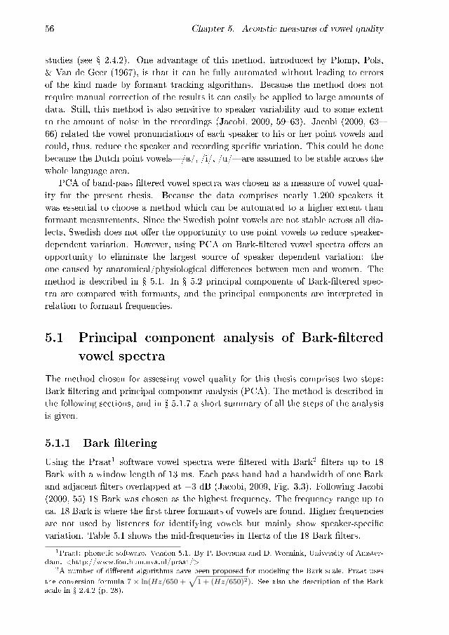
56 Chapter 5. Acoustic measures of vowel quality
studies (see � 2.4.2). One advantage of this method, introduced by Plomp, Pols,& Van de Geer (1967), is that it can be fully automated without leading to errorsof the kind made by formant tracking algorithms. Because the method does notrequire manual correction of the results it can easily be applied to large amounts ofdata. Still, this method is also sensitive to speaker variability and to some extentto the amount of noise in the recordings (Jacobi, 2009, 59�63). Jacobi (2009, 63�66) related the vowel pronunciations of each speaker to his or her point vowels andcould, thus, reduce the speaker and recording speci�c variation. This could be donebecause the Dutch point vowels�/a/, /i/, /u/�are assumed to be stable across thewhole language area.
PCA of band-pass �ltered vowel spectra was chosen as a measure of vowel qual-ity for the present thesis. Because the data comprises nearly 1,200 speakers itwas essential to choose a method which can be automated to a higher extent thanformant measurements. Since the Swedish point vowels are not stable across all dia-lects, Swedish does not o�er the opportunity to use point vowels to reduce speaker-dependent variation. However, using PCA on Bark-�ltered vowel spectra o�ers anopportunity to eliminate the largest source of speaker dependent variation: theone caused by anatomical/physiological di�erences between men and women. Themethod is described in � 5.1. In � 5.2 principal components of Bark-�ltered spec-tra are compared with formants, and the principal components are interpreted inrelation to formant frequencies.
5.1 Principal component analysis of Bark-�ltered
vowel spectra
The method chosen for assessing vowel quality for this thesis comprises two steps:Bark �ltering and principal component analysis (PCA). The method is described inthe following sections, and in � 5.1.7 a short summary of all the steps of the analysisis given.
5.1.1 Bark �ltering
Using the Praat1 software vowel spectra were �ltered with Bark2 �lters up to 18Bark with a window length of 13 ms. Each pass band had a bandwidth of one Barkand adjacent �lters overlapped at −3 dB (Jacobi, 2009, Fig. 3.3). Following Jacobi(2009, 55) 18 Bark was chosen as the highest frequency. The frequency range up toca. 18 Bark is where the �rst three formants of vowels are found. Higher frequenciesare not used by listeners for identifying vowels but mainly show speaker-speci�cvariation. Table 5.1 shows the mid-frequencies in Hertz of the 18 Bark �lters.
1Praat: phonetic software. Version 5.1. By P. Boersma and D. Weenink, University of Amster-dam. <http://www.fon.hum.uva.nl/praat/>
2A number of di�erent algorithms have been proposed for modeling the Bark scale. Praat usesthe conversion formula 7 × ln(Hz/650 +
√1 + (Hz/650)2). See also the description of the Bark
scale in � 2.4.2 (p. 28).
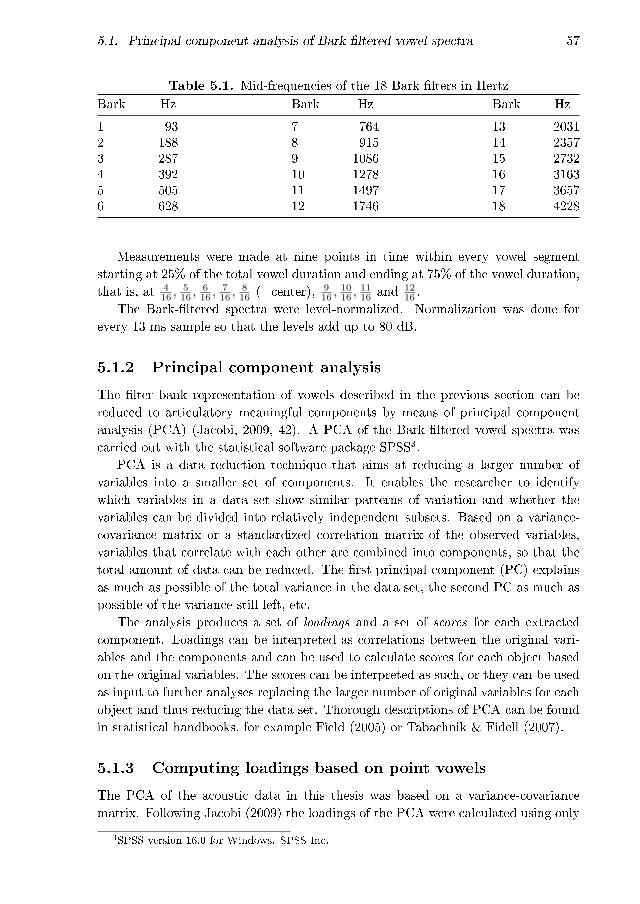
5.1. Principal component analysis of Bark-�ltered vowel spectra 57
Table 5.1. Mid-frequencies of the 18 Bark �lters in HertzBark Hz Bark Hz Bark Hz
1 93 7 764 13 20312 188 8 915 14 23573 287 9 1086 15 27324 392 10 1278 16 31635 505 11 1497 17 36576 628 12 1746 18 4228
Measurements were made at nine points in time within every vowel segmentstarting at 25% of the total vowel duration and ending at 75% of the vowel duration,that is, at 4
16 , 516 , 6
16 , 716 , 8
16 (=center), 916 , 10
16 , 1116 and 12
16 .The Bark-�ltered spectra were level-normalized. Normalization was done for
every 13 ms sample so that the levels add up to 80 dB.
5.1.2 Principal component analysis
The �lter bank representation of vowels described in the previous section can bereduced to articulatory meaningful components by means of principal componentanalysis (PCA) (Jacobi, 2009, 42). A PCA of the Bark-�ltered vowel spectra wascarried out with the statistical software package SPSS3.
PCA is a data reduction technique that aims at reducing a larger number ofvariables into a smaller set of components. It enables the researcher to identifywhich variables in a data set show similar patterns of variation and whether thevariables can be divided into relatively independent subsets. Based on a variance-covariance matrix or a standardized correlation matrix of the observed variables,variables that correlate with each other are combined into components, so that thetotal amount of data can be reduced. The �rst principal component (PC) explainsas much as possible of the total variance in the data set, the second PC as much aspossible of the variance still left, etc.
The analysis produces a set of loadings and a set of scores for each extractedcomponent. Loadings can be interpreted as correlations between the original vari-ables and the components and can be used to calculate scores for each object basedon the original variables. The scores can be interpreted as such, or they can be usedas input to further analyses replacing the larger number of original variables for eachobject and thus reducing the data set. Thorough descriptions of PCA can be foundin statistical handbooks, for example Field (2005) or Tabachnik & Fidell (2007).
5.1.3 Computing loadings based on point vowels
The PCA of the acoustic data in this thesis was based on a variance-covariancematrix. Following Jacobi (2009) the loadings of the PCA were calculated using only
3SPSS version 16.0 for Windows. SPSS Inc.

58 Chapter 5. Acoustic measures of vowel quality
Table 5.2. Sample of the four point vowels (measured at the temporal mid-point) ofa number of speakers used in the analysis phase of the PCA for computing loadings.bf = Bark �lter
objects variables
speaker vowelbf2 bf3 ... bfn(dB) (dB) (dB)
speaker1 a 58.60 61.10 ... 46.37æ 65.57 65.25 ... 64.85i 67.80 72.10 ... 68.49u 63.09 67.44 ... 56.73
speaker2 a 61.71 62.41 ... 41.85æ 71.94 73.89 ... 58.98i 69.23 72.27 ... 56.01u 67.96 70.28 ... 37.85
... ... ... ... ... ...
speakern a 59.97 61.52 ... 52.51æ 54.37 53.34 ... 57.02i 65.15 68.73 ... 59.00u 65.16 66.34 ... 38.82
Table 5.3. Sample of data to be reduced by the PCA. Each of the 19 vowels ofevery speaker is represented by the intensities (in dB) in a number of Bark �lters(bf) measured at nine sampling points within the vowel segments.
objects variables
speaker vowelpointbf2 bf3 ... bfn(dB) (dB) ... (dB)
speaker1 dis1 66.69 71.96 ... 64.31dis2 66.79 71.82 ... 63.48dis... ... ... ... ...dis9 72.62 75.57 ... 68.85disk1 73.24 75.72 ... 64.99disk... ... ... ... ...disk9 72.87 75.17 ... 65.57... ... ... ... ...typ1 67.26 73.04 ... 63.85typ... ... ... ... ...typ9 74.03 75.45 ... 62.56
... ... ... ... ... ...
speakern typ1 72.71 75.28 ... 52.36typ... ... ... ... ...typ9 75.51 75.83 ... 50.67

5.1. Principal component analysis of Bark-�ltered vowel spectra 59
point vowels (that is, vowels with the most extreme values for the two �rst formants).This is done in order to weigh all articulatory dimensions equally and to make surethat the PCA accounts for all possible variation in the vowel space. Table 5.2 showsa sample of the data used as input in this initial phase of the PCA. The point vowelsof the speakers serve as objects in the analysis, and the intensities of the Bark �ltersas variables.
For the Swedish data the vowels transcribed as [i:], [æ:], [A:]/[a:] and [u:] in thedatabase were chosen for computing the loadings in the initial phase of the PCA.Two variants were allowed for /A:/, since the pronunciation in Standard Swedishis [A:], but we did not want to exclude that even more open vowels were added tothe analysis. Standard Swedish [æ:] has a more extreme F1 than Swedish [A:] (seeTable 5.11, p. 83) and was therefore also used as a point vowel.
Some dialects show such strong deviation from Standard Swedish that not allpoint vowels could be found in the set of 19 words. For example, the South Swedishdialects have strongly diphthongized pronunciations of the long close vowels /i:/and /u:/. Because point vowels were not available for all of the speakers, a subsetof speakers was used for calculating the loadings. All point vowels were availablefor 230 women. The number of men with all point vowels was a bit larger, soout of these speakers 230 men were picked randomly, in order to include as manymen as women in the analysis. Using 230 men and 230 women for computing theloadings of the PCA, means that a great number vowel spaces with di�erent speaker-dependent sizes are included. Based on this, scores can be calculated also for thevowels of the speakers that were not included in the initial subset. Only the centralmeasurement point was used for calculating the loadings. For each of the 230 menand 230 women average levels of the Bark �lters of all occurrences of the point vowelswere calculated.4
Figure 5.1 shows the mean intensities per Bark �lter for the point vowels of the230 men and 230 women. In these �gures the characteristic spectra of the pointvowels can be identi�ed. The [i:] vowel has a very low �rst formant resulting in anintensity peak in the lowest frequency area, approximately at Bark �lters 2 and 3.The second formant of [i:] is very high, at approximately 13�15 Bark. The openvowel [æ:] has a high F1 at 6�7 Bark. The spectral peaks resulting from F2 and F3of [æ:] can also be seen clearly at 11�12 respectively 14�15 Bark. F1 and F2 of thevowel [A:]/[a:] are very close to each other giving a broad peak at 5�9 Bark, whilethe �rst two formants of [u:] are very close to each other as well, but at a muchlower frequency (3�7 Bark). The lines of men and women are very similar in thesegraphs but the peaks of the spectra are consistently at a somewhat higher frequencyfor women than men. This can be illustrated by shifting the frequency scale with1 Bark, which is done in Figure 5.2. In these �gures the lines of men and womenfollow each other almost perfectly.
The biggest di�erence between the spectra of men and women in Figure 5.2seems to be that the women in general have less intensity at the highest frequencies,
4Laverage = 10log10[( 1n
)∑n
i=1log−1(Li/10)]

60 Chapter 5. Acoustic measures of vowel quality
Bark filter
dB
0 2 4 6 8 10 12 14 16 18
3040
5060
7080
[i:]
menwomen
Bark filter
dB
0 2 4 6 8 10 12 14 16 18
3040
5060
7080
[u:]
Bark filter
dB
0 2 4 6 8 10 12 14 16 18
3040
5060
7080
[æ:]
Bark filter
dB
0 2 4 6 8 10 12 14 16 18
3040
5060
7080
[a:]
Figure 5.1. Average decibel levels of the point vowels in the band-pass �lteredfrequency regions.
which can be most clearly seen in the case of [i:]. The vocal folds of men and womenproduce a di�erent kind of pulse. The duration of the open portion of a fundamentalperiod is relatively longer in women's voices, and due to the relatively longer pulse bywomen than by men the higher harmonics are weaker in women's speech (Rietveld& Van Heuven, 2009, 341). This leads to a steeper spectral tilt for women thanfor men. Measured with four rather broad frequency bands Sluijter & Van Heuven(1996) found that at 0�500 Hz female voice have 1 dB greater intensity than malevoices, while at 500�4000 Hz the intensity is 2�3 dB weaker in female voices than inmale voices. The greater intensity of men than of women at the highest frequenciesin Figure 5.2 is therefore attested also in previous studies.
Van Nierop, Pols, & Plomp (1973) showed that the systematic di�erences in thespectra of vowels produced by men and women lead to similar results when carryingout separate PCAs for the two groups. The main latent variables related to vowelpronunciation are present in the acoustic data of both men and women, but theinformation is found at a higher frequency in the female data. This fact was usedin the current thesis for normalizing for the systematic di�erences in the acousticdata of men and women related to anatomy/physiology: separate PCAs were carriedout on the male data and the female data. The scores of the two separate PCAscan subsequently be used as comparable measures of vowel quality and can be used

5.1. Principal component analysis of Bark-�ltered vowel spectra 61
Bark filter (men)dB
0 2 4 6 8 10 12 14 16 1830
4050
6070
80
[i:]
menwomen
Bark filter (men)
dB
0 2 4 6 8 10 12 14 16 18
3040
5060
7080
[u:]
Bark filter (women)
dB
1 3 5 7 9 11 13 15 17 19
3040
5060
7080
[æ:]
Bark filter (women)
dB
1 3 5 7 9 11 13 15 17 19
3040
5060
7080
[a:]
Figure 5.2. Average decibel levels of the point vowels in the band-pass �lteredfrequency regions. Scales of men and women shifted with 1 Bark.
in analyses of dialectal variation. Bark �lters 2�17 were used as variables in thePCA of the male data and Bark �lters 3�18 in the female analysis. Using a setof Bark �lters shifted with 1 Bark as variables in the two analyses means that thefrequency area analyzed in the two PCAs contains the same information related tovowel pronunciation. Both analyses comprised 920 objects in the initial phase (4vowels × 230 speakers). In � 5.1.5 the e�ect of analyzing the female and male dataseparately is examined more closely.
Jacobi (2009) carried out one PCA, which included both female and male speak-ers. She combined the two lowest Bark �lters (1 and 2) in order to �prevent strongvariance caused by the speakers' varying fundamental frequency�. The mean funda-mental frequency of Swedish speakers has been shown to be 188 Hz for women and116 Hz for men (Pegoraro-Krook, 1988). Thus, the fundamental frequency is mainlyrepresented in the �rst Bark �lter for men and in the second for women. These Bark�lters are not important for identifying vowels. When analyzing data from men andwomen separately the lowest Bark �lters which represent the fundamental frequencycan be left out.
After computing the loadings of a PCA with a subset of objects, scores can becomputed for the full data set. Also the second phase of the PCA was carried outseparately for men and women. Table 5.3 shows a sample of the full data set used

62 Chapter 5. Acoustic measures of vowel quality
Table 5.4. Result of data reduction byPCA. The original variables (that is, theintensities in a number of Bark �lters)have been reduced to scores on two PCs.The objects of the analysis are the 19vowels of all speakers measured at ninesampling points.
speaker vowelpoint PC1 PC2
speaker1 dis1 -0.99 1.75dis2 -1.20 1.61dis... ... ...dis9 -2.15 1.62disk1 -1.56 1.76disk... ... ...disk9 -1.83 1.58... ... ...typ1 -1.02 1.79typ... ... ...typ9 -1.82 1.70
... ... ... ...
speakern typ1 -102 0.98typ... ... ...typ9 -1.31 0.96
as input in the second phase of the PCA. The objects of the full data set are the 19vowels (see � 4.2.1) of all (male/female) speakers measured at nine sampling points.Based on the loadings from the initial phase of each PCA scores for all vowels ofall male/female speakers were computed. Table 5.4 displays a sample of the scoreswhich are the output of the PCA. In the data set that has been reduced by means ofPCA each object is described by scores on two extracted components (PCs) insteadof by the original variables. These scores are the measures of vowel quality.
5.1.4 Rotating the solution
Because the �rst PC explains as much as possible of the total variance in the data set,most variables will have relatively high loadings on the �rst PC and smaller loadingson the remaining components. This can make interpretation of components di�cult,since the original variables are not necessarily unambiguously connected to only oneof the extracted components. This characteristic can be changed by using rotationtechniques.
The most commonly used rotation technique is varimax, which rotates the axesso that the variables correlate maximally with only one component. Figure 5.3shows the loadings of the two �rst PCs based on the male and female point vowelsin unrotated solutions. The plots show clouds of variables that are not centeredalong any of the axes, but the variables correlate with both the �rst and the secondPC. These are typical cases where rotation could lead to more easily interpretablesolutions.
Figure 5.4 shows the loadings of PCAs of the same data with varimax rotation.Contrary to Figure 5.3, the clouds of variables are now centered along the x- andy-axes and only a few variables correlate highly with both PCs. Interpretation of

5.1. Principal component analysis of Bark-�ltered vowel spectra 63
●●
●
●
●●●
●
●
●
●
●
●●
●●
−1.0 −0.5 0.0 0.5 1.0
−1.
0−
0.5
0.0
0.5
1.0
PC1
PC
2
23
4
56
78
9
10
11
12
13 1415
1617
men
●
●
●
●
● ●
●
●
●
●
●
●●
●
●●
−1.0 −0.5 0.0 0.5 1.0
−1.
0−
0.5
0.0
0.5
1.0
PC1P
C2
3
4
5
6 78
9
10
1112
13
141516
1718
women
Figure 5.3. Loadings on the two �rst PCs (men to the left, women to the right).The numbers indicate the number of the Bark �lters (men 2�17 Bark, women 3�18Bark).
●
●
●
●
●●
●
●
●
●
●● ●
●
●●
−1.0 −0.5 0.0 0.5 1.0
−1.
0−
0.5
0.0
0.5
1.0
PC1
PC
2
23
4
567
8
9
10
111213
1415
1617
men
●
●
●
●
●●
●
●
●
●
●
●●●
●●
−1.0 −0.5 0.0 0.5 1.0
−1.
0−
0.5
0.0
0.5
1.0
PC1
PC
2
34
56
789
10
11
121314 15161718
women
Figure 5.4. Loadings on two PCs extracted with varimax rotation (men to theleft, women to the right). The numbers indicate the number of the Bark �lters (men2�17 Bark, women 3�18 Bark).

64 Chapter 5. Acoustic measures of vowel quality
Bark filter
load
ing
2 4 6 8 10 12 14 16 18
−1.
0−
0.5
0.0
0.5
1.0
men PC1men PC2women PC1women PC2
Figure 5.5. Loadings of the male and female PCAs (2 PCs extracted withoutrotation) plotted against the frequency scale.
the components becomes easier because it is evident which variables correlate witheach of the PCs.5
Varimax also tends to equalize the proportion of variance explained by the com-ponents, by taking variance from the �rst component and distributing it among thelater ones (Tabachnik & Fidell, 2007, 638). Because of this all components will bea�ected by the number of components extracted when using varimax.
One further di�erence between the two pairs of plots in Figures 5.3 and 5.4 is thatthe con�gurations of the male and female analyses are mirrored around the x-axis inthe unrotated solutions in Figure 5.3; the highest band-pass �lters are found in thefourth quadrant in the male solution but in the �rst quadrant in the female solution,while the middle frequencies (Bark �lters 6�10) are in the �rst quadrant in the malesolution and in the fourth in the female solution. After applying varimax rotationthe solutions are much more similar for men and women (Figure 5.4). Van Nieropet al. (1973) found that solutions based on male data and female data are comparableand only need to be rotated in order to overlap each other. Varimax seems to o�era standard solution for rotation so that the con�gurations of male and female datahave the same orientation. Therefore, varimax was chosen as rotation technique forextracting the PCs for this thesis.
The di�erence between non-rotated solutions and solutions using varimax can beseen even more clearly when plotting the loadings along the frequency scale. Fig-ure 5.5 shows the loadings of the two �rst PCs of the male and female data extractedwithout rotation, while Figure 5.6 shows the loadings of the varimax solutions. While
5For an interpretation of the PCs, see � 5.2.3. See also � 5.2.1, where both the unrotated andthe rotated solutions are compared to formant measurements.

5.1. Principal component analysis of Bark-�ltered vowel spectra 65
Bark filter
load
ing
2 4 6 8 10 12 14 16 18
−1.
0−
0.5
0.0
0.5
1.0
men PC1men PC2women PC1women PC2
Figure 5.6. Loadings of the male and female PCAs (2 PCs extracted with varimaxrotation) plotted against the frequency scale.
Bark filter (men)
Bark filter (women)
load
ing
−1.
0−
0.5
0.0
0.5
1.0 2 3 4 5 6 7 8 9 10 11 12 13 14 15 16 17
3 4 5 6 7 8 9 10 11 12 13 14 15 16 17 18
men PC1men PC2women PC1women PC2
Figure 5.7. Loadings of the male and female PCAs (2 PCs extracted with varimaxrotation) plotted against a shifted frequency scale.
66 Chapter 5. Acoustic measures of vowel quality
2 1 0 −1 −2
21
0−
1−
2
PC2
PC
1
men
i
u
æ a
2 1 0 −1 −2
21
0−
1−
2
PC2
PC
1
women
i
u
æ a
Figure 5.8. Scores of the point vowels [i:], [æ:], [A:]/[a:] and [u:] in the PC2/PC1plane with varimax rotation. The plots of the male data (left) and female data(right) are similar to each other and resemble the IPA vowel quadrilateral. Onestandard deviation ellipses.
Figure 5.5 displays quite di�erent curves for men and women, the curves of the com-ponents in Figure 5.6 look very similar for both sexes. In the varimax solutionsthe loadings of men and women only seem to be placed di�erently on the frequencyscale.
In Figure 5.7 the frequency scale has been shifted so that instead of using thesame scale for men and women, the loadings of the male analysis are plotted on ascale ranging from 2 to 17 Bark, while the loadings of the female analysis are plottedon a scale from 3 to 18 Bark (which corresponds to the contiguous Bark �lters usedas variables in the two analyses). This �gure shows that the curves are indeed almostidentical for men and women after applying varimax, which suggests that the sameinformation is extracted in both PCAs. Because of the anatomical/physiologicaldi�erences between men and women this information can be found on average 1 Barkhigher in the female data.
The e�ect of applying varimax can also be visualized by plotting the scoresassigned to the point vowels by the PCA. The scores are the result of the datareduction, and can be used as measures of vowel quality for each segment. The scoreswere estimated with the regression method, which produces scores with a mean of 0and a standard deviation of 1 for each PC (Tabachnik & Fidell, 2007, 650). Figure 5.8shows the scores of the male and female point vowels in the varimax solution.6 Just
6Ellipses are drawn by applying PCA once more, but this time separately for each vowel withthe acoustic PCs as variables. The major and minor axes of the ellipses are the two �rst PCsof the data and the longest axis, hence, shows the direction that explains most of the variance(Harrington, 2010, Ch. 6). Assuming that the data is normally distributed an ellipse with a radiusof 1 standard deviation covers 39.4% of the data points, while an ellipse with a radius of 2 standarddeviations covers 86.5% of the data points. All ellipse plots in this thesis were drawn using the

5.1. Principal component analysis of Bark-�ltered vowel spectra 67
2 1 0 −1 −2
21
0−
1−
2
PC2
PC
1men
i
u
æ
a
2 1 0 −1 −2
21
0−
1−
2
PC2
PC
1
women
i
u
æ
a
Figure 5.9. Scores of the point vowels [i:], [æ:], [A:]/[a:] and [u:] in the PC2/PC1plane without applying any rotation technique. The vowel plots of the male data(left) and female data (right) show a skewed position compared to the plots inFigure 5.8 and are mirrored around the y-axis. One standard deviation ellipses.
as in a formant plot (see, for example, Figure 2.4, p. 25, and Figure 2.5, p. 30), thescores are plotted with the �rst component on the y-axis and the second componenton the x-axis with both scales reversed, which results in con�gurations that resemblethe IPA vowel quadrilateral. Figure 5.9, on the other hand, displays the scores ofthe point vowels of the unrotated PCAs. These plots do not show the familiar vowelquadrilateral with backness along the x-axis and height along the y-axis, but thevowel spaces have a rotated position in the coordinate system. Moreover, the plotsof the male and female point vowels are mirrored around the y-axis.
5.1.5 The result of separate PCAs of men and women
The result of analyzing the vowel pronunciations by men and women separately canbe examined by comparing the vowel scores. The plot to the left in Figure 5.10 showsthe scores of the point vowels after running separate PCAs for men and women withvarimax rotation. The ellipses, which have a radius of one standard deviation, �teach other almost perfectly.6
For comparison the plot to the right in Figure 5.10 shows the vowel scores of aPCA where men and women were included in the same analysis. Bark �lters 2�18were analyzed for all speakers, and the analysis included 1,840 objects (4 vowels ×460 speakers). Because the sexes were analyzed together the anatomical di�erencesbetween men and women led to systematic di�erences in the scores of the PCA.Vowels produced by women were assigned systematically higher scores on PC1 than
eplot() function of the Emu library in the software package R.

68 Chapter 5. Acoustic measures of vowel quality
2 1 0 −1 −2
21
0−
1−
2
PC2
PC
1
men and women analyzed separately
i
u
æ a
2 1 0 −1 −2
21
0−
1−
2
PC2
PC
1
men and women analyzed together
m:iw:i
m:uw:u
m:æw:æ
m:a
w:a
Figure 5.10. Scores of the point vowels [i:], [æ:], [A:]/[a:] and [u:] (2 PCs extractedwith varimax rotation). The plot to the left is based on separate PCAs for men andwomen, while the plot to the right is based on one PCA for speakers of both sexes.Separate one standard deviation ellipses are drawn for men (m) and women (w).The plot to the right fails to normalize vowel quality with respect to sex.
vowels produced by men. Separate analyses for men and women seem to normalizefor the anatomical di�erences.
In order to test to what extent separate PCAs for men and women actuallynormalize for the anatomical di�erences, t-tests were carried out for all four pointvowels. This was done both for the scores of the separate PCAs of men and womenand for the PCA that included both men and women. The t-values and the signi-�cance levels of the t-tests are displayed in Table 5.5. The results show that whencarrying out separate PCAs for men and women there are no signi�cant di�erencesbetween the scores of men and women except for on PC1 of [u:]. When runningonly one PCA where both men and women are included all vowels show signi�cantdi�erences on PC1, and [i:] and [u:] also on PC2. The separate analyses of men andwomen clearly leads to fewer di�erences between the sexes in the vowel scores.
Given that the separate analyses of vowels produced by men and women showless signi�cant di�erences between the sexes than one single analysis, we expect thatalso the total variance caused by speaker-speci�c variation is reduced by the separateanalyses. A visual impression is given by the plots in Figure 5.11, which show twostandard deviation ellipses of the point vowels of the 460 speakers (230 men and 230women) in the separate analyses and in the joined analysis. The size of the ellipsessuggests that a large amount of individual variation is still left after both analyses.However, the variation is reduced to some extent by analyzing men and womenseparately, as can most clearly be seen in the cases of [i:] and [u:]; the ellipses ofthese two vowels show overlap when men and women were analyzed together (rightplot in Figure 5.11) but no overlap when the PCA was carried out separately for the

5.1. Principal component analysis of Bark-�ltered vowel spectra 69
2 1 0 −1 −2
21
0−
1−
2
PC2
PC
1
men and women analyzed separately
i
u
æ a
2 1 0 −1 −2
21
0−
1−
2
PC2
PC
1
men and women analyzed together
i
u
æ a
Figure 5.11. Two standard deviation ellipses of the scores of the point vowels [i:],[æ:], [A:]/[a:] and [u:] (2 components extracted with varimax rotation). In the graphto the left, based on separate PCAs for men and women, the ellipses are smaller andshow less overlap than in the graph to the right based on one PCA for speakers ofboth sexes. Processing male and female voices separately, hence, reduces variability.
Table 5.5. T-tests comparing the means of female and male speakers on each pointvowel and on both PCs (df = 458).
separate PCAs for one PCAs for bothmen and women men and women
vowel value PC1 PC2 PC1 PC2
[i:] t −1.3 −0.4 −10.7 8.3sign. 0.191 0.671 <0.001 <0.001
[æ:] t −1.1 0.5 −9.0 −0.6sign. 0.254 0.608 <0.001 0.545
[A:]/[a:] t 0.1 −0.9 −17.7 −1.0sign. 0.895 0.380 <0.001 0.318
[u:] t 2.1 0.8 −9.7 3.3sign. 0.033 0.435 <0.001 0.001

70 Chapter 5. Acoustic measures of vowel quality
two speaker groups (left plot in Figure 5.11).The analyses above support the choice of carrying out separate PCAs for men
and women when reducing the �lter bank representation of vowels to articulatorymeaningful components. In order to further investigate which sources account forthe variance in the PCs multivariate analyses were carried out. The multivariateanalyses of PCs as well as of formant frequencies are presented in � 5.2.2.
5.1.6 E�ect of noise
Jacobi (2009, 59�63) found that the positioning of the vowel spaces of di�erentspeakers in the PC2/PC1 plane was a�ected by the signal-to-noise ratios in therecordings: the lower the signal-to-noise ratio (that is, the more noise), the smallerthe measured vowel space in the PC plane and the higher the PC scores. Jacobi'sdata comprised recordings in extremely varying situations from interviews in silentenvironments to private conversations and broadcast recordings with music in thebackground.
The present data set is much more homogeneous when it comes to the recordingsituations than Jacobi's data. In the SweDia project attention was payed to allrecordings being made in as similar circumstances as possible. The recordings weregenerally made in the speakers homes, and quiet rooms with as little reverberationas possible were chosen to ensure good recording quality (see � 4.1). Because nodrastically varying signal-to-noise ratios were expected in the present data the e�ectof noise in the dialect recordings was not tested.
The speakers representing Standard Swedish, however, were not recorded in theirhomes, but in a studio. A studio is more silent than any home environment, whichmeans that a higher signal-to-noise ratio could be expected for the speakers of Stand-ard Swedish than for the dialect speakers. The speakers of Standard Swedish werenot included in the initial subset used for calculating the loadings of the PCAs, butonly included in the full data set for which scores were calculated. As mentionedearlier the regression technique, used for calculating the scores in the PCA, producesscores with a mean of 0 and standard deviation of 1 for each PC. To test whether thestandard speakers had systematically lower scores than the dialect speakers, with apresumably lower signal-to-noise ratio, t-tests were carried out. The average scoreson both PCs of the standard speakers' four point vowels ([i:], [æ:], [A:]/[a:] and [u:])were tested against the point vowels of the 460 dialect speakers of the initial subset.For the dialect speakers the mean of both PCs was < 0.001 as expected. For thespeakers of Standard Swedish the mean of PC1 was −0.339 and the mean of PC2−0.273. For both PCs the di�erence between dialect speakers and standard speakerswas signi�cant (PC1: t(1886) = −2.30, p = 0.021; PC2: t(1886) = −1.86, p = 0.063).
As found by Jacobi (2009) a lower signal-to-noise ratio seems to lead to higherPC scores. Since the PCs are not comparable across the two di�erent recordingenvironments, the speakers of Standard Swedish were not included in any of thestatistical analyses in Chapters 6 and 7. The Standard Swedish pronunciation isonly included in the maps of each vowel in Appendix C.

5.2. Principal components versus formants 71
5.1.7 Summary of the acoustic analysis
In Figure 5.12 all the steps of the acoustic analysis of the vowel data are summarized.The acoustic analysis includes two steps which have been described above: 1) Bark�ltering, and 2) data reduction of the Bark-�ltered data with PCA. In a �nal stepbefore analyzing dialectal variation in the vowels group averages of groups of speakersare calculated.
The Bark �ltering was done at nine sampling points in each vowel segment andthe Bark-�ltered spectra were level-normalized to 80 dB. Since all speakers hadrepeated each of the 19 elicited vowels 3�5 times during the interviews, averagedB levels of the Bark �lters were calculated per vowel per sampling point for eachspeaker. After the Bark �ltering and the averaging, each of the 19 vowels of eachspeaker is represented by the average level-normalized intensities in the Bark �ltersat 9 sampling points.
In the data reduction phase the data was split up according to speaker-sex.Separate PCAs were carried out for women and men with Bark �lters 2�17 used asvariables in the male analysis and Bark �lters 3�18 in the female analysis. The PCAincludes computing loadings based on point vowels, and subsequently computingscores for all of the 19 vowels. After the PCA each of the 19 vowels of each speakeris represented by two PCs at the 9 sampling points instead of by the dB levels in thefrequency bands. The PCs of men and women are the output of two separate PCAs,but the scores are comparable because they represent the same latent variables inthe vowel spectra.
As explained in � 4.3 three di�erent groupings of the speakers in the data set areused in the analysis of dialectal variation in this thesis: a) one group per site, b)older and younger speakers per site, and c) older women, older men, younger women,and younger men per site. For the analyses in the following chapters of this thesis,arithmetic group means were calculated for PC1 and PC2 respectively for each ofthe 19 vowels at the nine sampling points. After this averaging the pronunciation ofthe 19 vowels of each speaker group is represented by two PCs at 9 sampling points.
5.2 Principal components versus formants
Since formant measurements have a much longer tradition in variationist linguisticsthan the use of PCs of Bark-�ltered spectra, a comparison of the PCs was madewith formants. This comparison was also used for �nding the optimal number ofPCs to extract.
Formants were measured for a subset of the SweDia data. Three sites werepicked randomly: Ankarsrum, Malung and Skog. Formants were measured for allspeakers from these sites. The data sets from Ankarsrum and Skog were completewith three speakers in each speaker group (older women, older men, younger womenand younger men). From Malung, however, one young man was missing in the dataset, which means that formants were measured for 18 women and 17 men in total.The formants were measured for the vowels in the stressed syllables of the words

72 Chapter 5. Acoustic measures of vowel quality
Bark filtering ofdigital speech samplesat 9 sampling points
in each vowel segment
level normalizationof each sample
to 80 dB
calculation of average dB levelsper sampling point and Bark filter
of the 3–5 repetitions byeach speaker of each vowel
each of the 19 vowels of each speakeris represented by the intensities in a
number of contiguous frequencybands at 9 sampling points
men:PCA with varimax rotation
objects: 9 sampling points of each of the 19 vowels of each speaker
variables: Bark filters 2–17
women:PCA with varimax rotation
objects: 9 sampling points of each of the 19 vowels of each speaker
variables: Bark filters 3–181) compute loadings on the temporal midpoint ofpoint vowels of a subsetof the male spakers
2) compute scores for all vowels of all male speakers
1) compute loadings onthe temporal midpoint ofpoint vowels of a subsetof the female spakers
2) compute scores for all vowels of all female speakers
each of the 19 vowels ofeach speaker is represented
by PC1 and PC2 at9 sampling points
data
redu
ctio
n by
PC
AB
ark
filte
ring
anal
ysis
of d
iale
ctal
var
iatio
n one speaker group per site(c. 12 speakers:
6 men and 6 women)
two groups per site: old and young
(c. 6 speakers per group:3 men and 3 women)
four groups per site: old men and women, and young men and women(c. 3 speakers per group)
calculationof arithmetic
group meansfor PC1 and PC2of each of the 19vowels at each
samplingpoint
analysesof geographic
and social variationin vowel pronun-
ciation
each of the19 vowelsof each
speaker groupis represented
byPC1 and PC2
at9 sampling
points
Figure 5.12. Work �ow of the acoustic analysis.

5.2. Principal components versus formants 73
described in � 4.2.1: dis /i:/, disk /I/, dör /œ:/, dörr /œ/, �ytta /Y/, lass /a/, lat/A:/, leta /e:/, lett /efl/, lott /O/, lus /0:/, lås/låt /o:/, lär /æ:/, lös /ø:/, nät /E:/,sot /u:/, särk /æ/, söt /ø:/, typ /y:/. In addition, the vowel /8/ elicited with theword ludd was used. In Ankarsrum låt was used to elicit /o:/, while lås was usedin Malung and Skog. One instance of every elicited vowel was measured for each ofthe speakers, which led to a total of 360 vowel pronunciations by women and 336 bymen.7
The �rst three formants were measured in the center of each segment with theformant track function in the EMU8 software. The window length was 25 ms andthe window type Blackman. The nominal F1 value was set to 500 Hz for the malespeakers and to 630 Hz for the female speakers. All measurements were inspectedand errors made by the formant tracker were corrected manually.
5.2.1 Correlation with formants
Jacobi (2009, Ch. 3) found high correlations between PCs of Bark-�ltered vowelspectra and formant measurements. The correlations are displayed in Table 5.6.The study was based on pronunciations of the Dutch phonemes /a/, /i/, /u/, /E/and /Ei/ by six female and six male speakers, measured close to onset and closeto o�set (2,767 speech segments in total). In a second study (Jacobi, 2009, Ch. 4)including more speakers (35 female and 35 male) and more vowel tokens (12,400) anda di�erent set of vowels (Dutch /o:/, /e:/, /Ei/, /Au/ and /œy/) Jacobi found thatthe correlations were somewhat lower: PC1�F1 r = 0.70, PC2�F2 r = 0.72. In thesestudies, the formants were measured automatically without manual correction ofthe measurements, which means that the correlations were based on partly incorrectformant values. With corrected formant measurements we can expect to �nd evenhigher correlations. Moreover, Jacobi (2009) did not use any rotation technique tooptimize the PC solution. Rotating the solution might in�uence the correlationsbetween formants and components.
Table 5.6. Correlations between formants and PCs of Bark-�ltered spectra foundby Jacobi (2009, Table 3.2, p. 38).
correlations expl. var.
F1 F2 F3 cum.PC Bark Bark Bark % %
PC1 0.81 −0.12 0.26 65 65PC2 −0.08 0.70 0.10 25 90PC3 −0.19 0.05 −0.15 5 95
7Four male speakers were missing one of the target vowels, which explains the total of 336 vowelsinstead of the expected 340 for the male data
8The EMU Speech Database System. Version 2.1.1. By the Institute of Phonetics and SpeechProcessing, LMU Munich. <http://emu.sourceforge.net/>
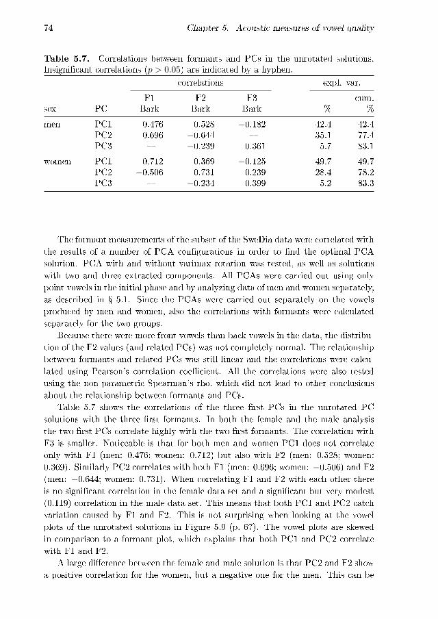
74 Chapter 5. Acoustic measures of vowel quality
Table 5.7. Correlations between formants and PCs in the unrotated solutions.Insigni�cant correlations (p > 0.05) are indicated by a hyphen.
correlations expl. var.
F1 F2 F3 cum.sex PC Bark Bark Bark % %
men PC1 0.476 0.528 −0.182 42.4 42.4PC2 0.696 −0.644 � 35.1 77.4PC3 � −0.239 0.361 5.7 83.1
women PC1 0.712 0.369 −0.125 49.7 49.7PC2 −0.506 0.731 0.239 28.4 78.2PC3 � −0.234 0.399 5.2 83.3
The formant measurements of the subset of the SweDia data were correlated withthe results of a number of PCA con�gurations in order to �nd the optimal PCAsolution. PCA with and without varimax rotation was tested, as well as solutionswith two and three extracted components. All PCAs were carried out using onlypoint vowels in the initial phase and by analyzing data of men and women separately,as described in � 5.1. Since the PCAs were carried out separately on the vowelsproduced by men and women, also the correlations with formants were calculatedseparately for the two groups.
Because there were more front vowels than back vowels in the data, the distribu-tion of the F2 values (and related PCs) was not completely normal. The relationshipbetween formants and related PCs was still linear and the correlations were calcu-lated using Pearson's correlation coe�cient. All the correlations were also testedusing the non-parametric Spearman's rho, which did not lead to other conclusionsabout the relationship between formants and PCs.
Table 5.7 shows the correlations of the three �rst PCs in the unrotated PCsolutions with the three �rst formants. In both the female and the male analysisthe two �rst PCs correlate highly with the two �rst formants. The correlation withF3 is smaller. Noticeable is that for both men and women PC1 does not correlateonly with F1 (men: 0.476; women: 0.712) but also with F2 (men: 0.528; women:0.369). Similarly PC2 correlates with both F1 (men: 0.696; women: −0.506) and F2(men: −0.644; women: 0.731). When correlating F1 and F2 with each other thereis no signi�cant correlation in the female data set and a signi�cant but very modest(0.119) correlation in the male data set. This means that both PC1 and PC2 catchvariation caused by F1 and F2. This is not surprising when looking at the vowelplots of the unrotated solutions in Figure 5.9 (p. 67). The vowel plots are skewedin comparison to a formant plot, which explains that both PC1 and PC2 correlatewith F1 and F2.
A large di�erence between the female and male solution is that PC2 and F2 showa positive correlation for the women, but a negative one for the men. This can be

5.2. Principal components versus formants 75
Table 5.8. Correlations between formants and PCs in the varimax solutions withthree components extracted. Insigni�cant correlations (p > 0.05) are indicated by ahyphen.
correlations expl. var.
F1 F2 F3 cum.sex PC Bark Bark Bark % %
men PC1 0.841 −0.443 � 39.0 39.0PC2 � 0.489 0.152 27.4 66.4PC3 0.181 0.522 −0.384 16.7 83.1
women PC1 0.819 −0.442 −0.135 38.1 38.1PC2 � 0.504 0.345 25.3 63.4PC3 0.250 0.533 −0.326 19.9 83.3
Table 5.9. Correlations between formants and PCs in the varimax solutions withtwo components extracted. Insigni�cant correlations (p > 0.05) are indicated by ahyphen. These solutions have the strongest association between PC1 and F1 andbetween PC2 and F2.
correlations expl. var.
F1 F2 F3 cum.sex PC Bark Bark Bark % %
men PC1 0.880 −0.352 −0.185 41.1 41.1PC2 � 0.732 � 36.3 77.4
women PC1 0.875 −0.360 −0.277 41.4 41.4PC2 0.152 0.744 � 36.8 78.2
compared to the mirrored scores in Figure 5.9 (p. 67) and the mirrored loadings inFigure 5.3 (p. 63).
When using varimax rotation, the number of components extracted in�uences allfactors (see � 5.1.4). Tables 5.8 and 5.9 show the correlations of the rotated solutionswhen extracting three and two components respectively. In the solution with threecomponents (Table 5.8) PC1 explains 39.0% of the variance for men and 38.1% forwomen. In the unrotated solutions in Table 5.7 the amount of explained varianceon PC1 is considerably higher (men: 42.4%; women: 49.7%). The total amount ofvariance explained by three PCs, however, is the same (men: 83.1%; women: 83.3%).Because varimax maximizes the variance of the loadings within the extracted PCs,the relative importance of the PCs is equalized.
In the varimax solution with three components (Table 5.8) PC1 and F1 correlatemore strongly with each other than in the unrotated solution (men: 0.841; women:0.819). On the other hand, all three extracted components correlate considerablywith F2 and there are only modest correlations between the PCs and F3. PCA doesnot seem to be able to completely separate the �rst three formants.

76 Chapter 5. Acoustic measures of vowel quality
When extracting two components with varimax rotation the pairwise correlationsbetween PC1 and F1 on the one hand, and PC2 and F2 on the other are considerablyhigher than in the other solutions (see Table 5.9). These correlations are also higherthan the ones found by Jacobi (2009) (Table 5.6). F1 and PC1 correlate at a level of0.88 for both men and women, and the correlation between F2 and PC2 is 0.73�0.74.PC1 also partly explains variation caused by F2 and F3.
When analyzing dialectal variation it is interesting to be able to draw articulatoryconclusions about vowel pronunciation. The varimax solutions with two extractedcomponents (Table 5.9) show the strongest direct relationship between PC1 and F1on the one hand and PC2 and F2 on the other. As can be seen in Figure 5.8 (p. 66)this solution also gives scores that correspond to the traditional vowel quadrilateralwhen plotting the scores in the PC2/PC1 plane. Because this model gave the highestcorrelations with formant measurements, it was chosen to be used throughout thisthesis for analyzing dialectal variation.
Figure 5.13 shows scatter plots of PC1 versus F1 and PC2 versus F2 of thevarimax solutions with two extracted components, with separate regression linesfor men and women. The linear relationship between F1 in Bark and PC1 is verystrong. F2 and PC2 show a somewhat less strong relationship. The cloud is denserfor high PC2/F2 values than for low values, which re�ects the fact that the datacomprises more front vowels than back vowels. But especially for the highest F2values, PC2 is in some cases lower than expected. While, F1 can be well predictedfrom PC1, PC2 apparently includes other spectral information than F2 only (seefurther � 5.2.3). Because of the strong relationship between PC1 and F1, PC1 canroughly be interpreted as representing vowel height. PC2 represents vowel backnessto some extent, but the articulatory conclusions based on PC2 should not be asstrong as those made for PC1.
Jacobi (2009) measured high pairwise correlations between formants and PCswithout using any rotation technique when extracting the PCs. One reason forthis could be that the Dutch point vowels are di�erent from the Swedish ones.Furthermore, the correlations of Jacobi (2009) are based on only �ve di�erent vowels,while the current study includes 20 di�erent vowel phonemes. This means that thecorrelations in the current study are based on a more varied and more continuousdata set even though the total number of tokens is smaller. Because of this, theresults of the two studies are not directly comparable to each other.
Even though the correlations with formant measurements are high one shouldstill bear in mind that using band-pass �ltering means that rather broadly de�nedfrequency regions determine the representation of vowel quality. Some �ner di�er-ences in formant frequencies between language varieties, possible to �nd by manualanalysis and correction, may be lost. One advantage of using PCA of Bark-�lteredspectra, however, is that the method can be completely automated, which makes itsuitable for analyzing large data sets.

5.2. Principal components versus formants 77
●
●
●●
●
●
●
●●●
●
●
●●
●●
●
●
●
●
●
●
●●
●●
●●
●
●
●●
●
●
●
●
●
●
●
●
●●
●
●●
●
●
●
●●
●
●●●
●●
●
●
●●
●
●●
●
●
● ●
●
● ●
●
●
●
●
● ●
●
●●
●
●
●
●
●●
● ●
●●
●●
●●
●
●
●
●
●
●
●
●
●
●
●
●
●
●
●
●
●
●
●●
●
●
●●
●
●
●
●
●
●
●
●
●
●●
●
●●●
●●
●
●●
●
●
●
●●
●
●●
●
●●
●
●
● ●
●
●
●
●
●
●
●
●
●●
●
●
●
●
●
●●
●
●
●
●
●
●
●
●●
●
●
●●
●
●
● ●
●
●
●
●
●
●
●
●
●
●
●
●●
●
●
●
●
●
●●●
●
●
●
●●
●●
●
●
●
●
●
●●
●●
● ●
●
●
●
●
●
●
●
●●
●
●●
●
●
● ●
●
●
●
●
●
●
●●
● ●
●●
●
●
●
●● ●
●
●
●●● ●
●●● ●
●
●
●
●
●●● ●
●
●
●
●●
●
●●
●
●
● ●
●
●●
●●
●
●
●
●
●
●
● ●●
●
●
●
●●
●
●●●
●
●●
●●
●
●●●
●
●
●
●●●
●
●
●
● ●
●
●●
●
−2 −1 0 1 2
24
68
PC1
F1
(Bar
k)
●
●
●
●
● ●
●
●
●
●●
●
●
●
●
●●
●
●
●
●
●●
●
●
●
●
●
●●
●
●
●
●
●
●
●
●
●●
●
●
●
●
●
●
●
●
●
●
●
●
●
●
●●
●
●
●
●
●
●
●
●●
●
●●
●
●●
● ●
●
● ●
● ●
●
●
●
●
●
●
●●
●
●
●
●
●
●
●
●
●
●
●
●
●
●
●
●
●
●
●●
●
●
●
●
●●
●
●
●
●
●
●●
●
●
●
●●
●
●
●
●●
●●
●
●
●
●●
●●
●
●
●● ●
●
●
●
●
●
●●
●
●
●
●●
●
●
●●
●
●
●
●●
●
●
●
●
●●
●
●●
●
●
●
●
●
●
●
●
●
●
●●
●
●
●
●
●
●
●●
●●
●
●
●
●
●●
●
●●
●
●
●
●
●
●
●●
●
●●
● ●
●
●
●
●●
●
●●
●
●
●
●
●
●
●●
●
●
●
●
●
●
●
●
●
●
●
●
●
●
●
●●
●●
●
●
●
●
●
●
●
●
●
●●
●
●
●
●
● ●●
●
●
●
●
●
●
●●
●
●
●
●
●
●
●
●●
●
●
●●
●
●●
●
●
●
●
●
●●
●●
●
●
●
●
●
●
●●
●
●
●
● ●
●●
●●
●
●●●
●
●
●
●
●
●
●
●
●
●
●
●
●
●
●
●
●
●
●
●
●
●
●
●
●
●
●
●●
●
●
●
●
●
●●
●
●
men (r² = .775)women (r² = .765)
●● ●
●
●
●
●●
●
●●
●
●●●
●●●
●
●
●
●● ●
● ●
●
●
●
●
●
●●
●
●
●
●
● ●●
●●
●●
●
●
●
●●●
●
●
●
●
●
●
●
●
● ●
●
●
●
●
●
●
●●
●●
●
●
●●●
●●
●
●
●
●
●
●●●
●
●●
●
●
●●
●●
●
●
●●
●
●
●
●
●
●
●●
●● ●
●
●
●
●
●
●●
●
●
●
●
●●
●
●●
●●
●
●
●●
●●
●
● ●
●
●
●
●
●
●
●
●
●
●● ●
●●
● ●
●
●
●
●
●●●
●
●
●●
●
●
●●●
●
●●●
●
●
●
●
●
●
●●●
●●
●●
●●
●
●
●
● ●
●
●●
● ●
●●
●
●
●
●
●
●●
●●
●
●
●
●
●
●
●●
●
●●
●
●
●●
●
●
●
●
●●
●
● ●●
●
●
●
●
●
●
●
●
●●
●
●
●●
● ●●
●
●
●
●
●
●●
●
●
● ●
●
●
●
●
●●● ●
●●
●
● ●
●
●
●
●
●
●
●●
●
●
●
● ●
●
●
●
●●
●●
● ●●
●●
●
●
●●
●
●
●
●●
●
●●
●
●
●
●
●
●
●
●
●
●
●●
●
●
●●
●
●
●
● ●●
●
●●
−2 −1 0 1 2
46
810
1214
16
PC2
F2
(Bar
k)
●
●
●
●
●
●
●● ●
●
●
●
●
●
●
●
●
●
●
●
●
●
●
●
●
●
●
●●
●
●
●
●●
●
●
●●
●●
●
●
● ●
●
●●●
●
●
●●
●
●
●
●●●
●
●
●
●
●●
●
●
● ●
● ●
●
●
●
●
●
●●
●
●
●
●
●
●●
●
● ●
●
●
●
●
●
●●
●
●
●●
●
●
●
●
●
●
●●
●
●
●
●
●
●
●
●
●
●
●●
●
● ●
●
●
●
●●
●
●
●
●●●
●
●
● ● ●
●
●
●●
●
●
●
●
●●
●
●●
●●
●
●
●
●
●
●●
●
●
●
●
●●
● ●
●
●
●● ●
●
●
●
●
●
●●
●
●
●
●●
●
●●
●
●
●
●
●
●●
●
●
●
●
● ●
●●
●
● ●
●
●
●
●
●
●
●
●●
●
●
●
●
●
●
●●
●
●
●
●
●
● ●
●●
●
●
●
●
●
●
●●
●
●●
●
● ●
●●
●●
●
●●
●
●
●
●
●
●
●●
●
●●
●
●
●●
●●
●
●
●
●
●●
●
●●
●
●●
●
●
●
●
●
●
●
●●
●
●
●
●
●
●
●
●
●
●
●
●●
●●
●
●
●
●
●
●●
●
●●
●●
●
●●●
●
●
●
●
●
●
●
●●
●
●
●
● ●
●
●
●
●
●
●
●
●
●
●●
●
●
●
●
●
●
●●
●●
● ●
●
●
●
●
men (r² = .536)women (r² = .553)
Figure 5.13. Scatter plots of PCs (2 components extracted with varimax rotation)versus formants. Regression lines are drawn separately for men and women. PC1shows a better �t with F1 than PC2 with F2.

78 Chapter 5. Acoustic measures of vowel quality
Table 5.10. Results of the four multivariate analyses of variance: η2 for eachsigni�cant factor (p < 0.05).
η2 F1-F2 F1-F2-F3 PC1-PC2 PC1-PC2Bark Bark joined analysis sex separated
vowel 0.875 0.743 0.735 0.750speaker-sex 0.499 0.690 0.193 0.024site 0.038 0.054 0.062 0.066vowel*speaker-sex 0.091 0.069 0.060 �vowel*site 0.346 0.278 0.240 0.257speaker-sex*site � 0.031 0.069 0.066vowel*speaker-sex*site � � � �
5.2.2 Multivariate analysis
One further way of comparing PCA of Bark-�ltered vowel spectra with formantfrequencies is to analyze to what extent the methods are able to separate di�erentsources of variation in the data. This was done by carrying out manovas with themeasures of vowel quality as dependent variables and vowel, site and speaker-sexas independent variables. Four di�erent manovas were carried out with di�erentdependent variables:
1. F1 and F2 measured in Bark
2. F1, F2 and F3 measured in Bark
3. two PCs extracted using varimax rotation separately for men and women
4. two PCs extracted using varimax rotation including men and women in onesingle PCA
In order to make the data as normally distributed as possible a few front vowels(the vowels elicited with the words disk, leta, nät, särk and typ) were left out of theanalysis. The independent variables of the analyses were vowel (with 15 categories),speaker-sex (men and women), and site (Ankarsrum, Malung, Skog). The totalnumber of speakers was 35 (17 men and 18 women), and the number of vowel tokenswas 523 (due to a few instances of missing records). The signi�cance level wasestimated using Pillai's trace and the e�ect size was estimated by η2, which showsthe proportion of the total variance in the dependent variables accounted for by theindependent variables. Table 5.10 shows the η2 values of the signi�cant results ofthe four manovas.
As expected all analyses show a signi�cant main e�ect of vowel. The e�ect size ofvowel is largest for the analysis with F1 and F2 as dependent variables (η2 = 0.875).The e�ect size decreases when adding F3 to the analysis (η2 = 0.743). This can becompared with the results of Adank (2003, 99�102), who used manova to comparethe e�ect of a number of speaker normalization procedures. Her data consisted ofrecordings of the Dutch vowel phonemes by 160 speakers of Standard Dutch from

5.2. Principal components versus formants 79
eight di�erent geographic regions in the Netherlands and Flanders with an equaldistribution of female and male and older and younger speakers. Adank found ane�ect size of η2 = 0.893 for vowel when using two formants measured in Hertz as de-pendent variables, and η2 = 0.695 with three formants as dependent variables. Thebest performing normalization procedure, Lobanov's (1971) z -normalization, gave avowel e�ect of η2 = 0.932 with two normalized formants as dependent variables andη2 = 0.760 with three normalized formants as dependent variables.
The main e�ect of vowel is smaller in the manovas with PCs as dependent vari-ables than when using the �rst two formants. The sex separated PCA (η2 = 0.750)gives a somewhat larger e�ect of vowel than the PCA where men and women wereanalyzed together (η2 = 0.735) and also larger than when using three formants.
The formant-based manovas show a large main e�ect of speaker-sex. With threeformants (η2 = 0.690) this e�ect is even larger than with two (η2 = 0.499), which wasalso found by Adank (2003, 101�102). F3 seems to have even more sex-dependentvariance than F1 and F2, which explains why the main e�ect of vowel decreaseswhen adding F3 to the analysis.
In the PCs the e�ect of speaker-sex is much smaller than in formants. Whenmen and women were analyzed separately there is hardly any e�ect of speaker-sexin the measurements of vowel quality (η2 = 0.024), which con�rms the results of� 5.1.5. But also a PCA that includes both men and women gives a smaller e�ectof speaker-sex than formants measured in Bark (η2 = 0.193).
Jacobi (2009, 57) measured the area of /i � a � u/ vowel triangles of men andwomen based on formant measurements in Bark as well as PCs of Bark-�lteredspectra. The formant measurements in Bark showed a signi�cant di�erence in thesizes of the vowel spaces of men and women. The PCs, on the other hand, did notshow any signi�cant di�erence in the size of the vowel spaces of men and women;only the position of the vowel triangles di�ered between men and women in the PCplane.
Applying PCA separately to men and women sets the mean of both groups tozero, which means that there is a correction for the di�erent positions of the vowelspaces in the PC plane. Some speaker-speci�c variation is still left, but the biggestfactor, sex, is removed.
Using the �rst two formants for measuring vowel quality seems to lead to a bet-ter separation of vowels than in principal component solutions. However, formantmeasurements show large di�erences between men and women. The speaker andsex speci�c variation in formant measurements can be reduced by applying normal-ization procedures (see � 2.4.4). But successful speaker normalization proceduresare generally based on the average and/or standard deviation of the vowel phon-emes, which makes comparison of language varieties with di�erent phoneme systemsor di�erent vowel centers di�cult. Using PCA on Bark-�ltered spectra does notremove all speaker-speci�c variation in vowel pronunciation, but by applying PCAseparately to male and female data the systematic di�erences caused by the ana-tomical/physiological di�erences between the sexes can be diminished. Moreover, aPCA can be built up on point vowels of a number of speakers and subsequently ap-

80 Chapter 5. Acoustic measures of vowel quality
plied to a larger data set. Because of this, varieties with di�erent phoneme systemsand/or varieties lacking some of the point vowels can be compared to each other.This is an important precondition when comparing Swedish dialects, some of whichhave phoneme systems that deviate strongly from Standard Swedish.
5.2.3 Interpreting principal components
PCA of Bark-�ltered vowel spectra was shown to correlate highly with formantsin � 5.2.1. Exactly how the combination of a number of pass bands can result in acon�guration so similar to formants is not completely straightforward to understand.
Pols (1977) applied PCA to band-pass �ltered vowel spectra and wrote (p. 49):�This mathematically well-de�ned factor representation is not as easy to interpretas a formant representation.� Pols (1977, 49�50) compared vowel spectra with theloadings of the PCA in order to explain the coordinate values of the vowels in thePC plane. This is also what is done in Figure 5.14; the average spectra of the pointvowels are compared with the loadings of the extracted PCs. The �gure is basedon male speakers only, but it would look the same when based on female speakers,as is evident from Figures 5.2 (p. 61) and 5.7 (p. 65). Loadings > 0.6 and < −0.6on the PCs are marked with a symbol. This shows that frequencies up to 10 Barklargely determine PC1, with negative correlations with the two �rst Bark �lters andpositive correlations with Bark �lters 4�10. Frequencies above 11 Bark are the mostimportant ones determining PC2.
The lines of the open vowels [æ:] and [A:]/[a:] are similar to the one of PC1 instarting low at the two �rst Bark �lters and having a peak at 5�6 Bark. From thisfollows that they will have high positive scores on PC1. The close vowels [i:] and[u:], on the other hand, show more of a mirrored curve of the loadings of PC1 atthe lower frequency regions. They start high but fall soon. Because they show themirror of the loadings of PC1 they will get negative scores on this component.
The back vowels [u:] and [A:]/[a:] have a low F2 at about 6�8 Bark. BecauseF2 is low there is only little energy in the higher frequency areas determining PC2.Accordingly, these vowels are assigned negative scores on PC2. The front vowels [i:]and [æ:], on the other hand, have a high F2; [i:] around 13 Bark and [æ:] around11 Bark. Thus, the second formant of the front vowels falls in the higher frequencyregions that largely determine PC2. High energy levels in this frequency area leadto high scores on PC2. This reasoning is con�rmed by looking at the scores of thepoint vowels in Figure 5.8 (p. 66).
Some more insight can by acquired by looking at the interactions of PC1 andPC2 at the frequency areas of the formants. Table 5.11 shows the loadings of the twoPCs of the male analysis. Additionally the table indicates within which Bark �lterthe average formant frequencies of Swedish long vowels produced by male speakers(Eklund & Traunmüller, 1997) are placed.9
9Since average formant frequencies are used, one should bear in mind that the actual variationspreads across the given Bark �lters.
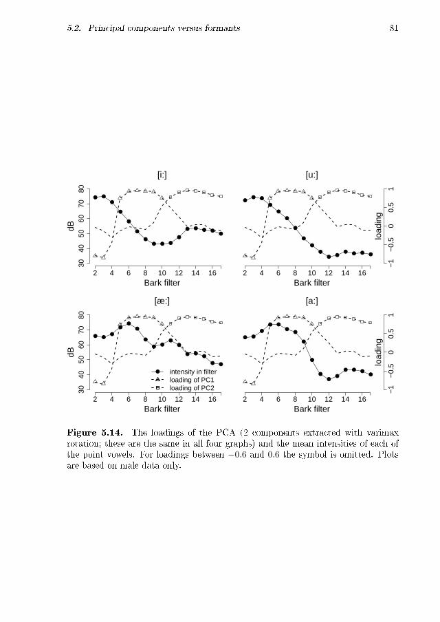
5.2. Principal components versus formants 81
[i:]
Bark filter
dB
2 4 6 8 10 12 14 16
3040
5060
7080
● ●
●
●
●
●
●● ● ●
●
● ● ● ●●
[u:]
Bark filter2 4 6 8 10 12 14 16
−1
−0.
50
0.5
1
●● ●
●
●
●
●
●
●
●● ●
● ● ● ●
load
ing
[æ:]
Bark filter
dB
2 4 6 8 10 12 14 16
3040
5060
7080
● ●●
●●
●
●
● ●●
●
● ●●
● ●
● intensity in filterloading of PC1loading of PC2
[a:]
Bark filter2 4 6 8 10 12 14 16
−1
−0.
50
0.5
1
● ●
●
● ●●
●
●
●
●
●●
● ● ●●
load
ing
Figure 5.14. The loadings of the PCA (2 components extracted with varimaxrotation; these are the same in all four graphs) and the mean intensities of each ofthe point vowels. For loadings between −0.6 and 0.6 the symbol is omitted. Plotsare based on male data only.
82 Chapter 5. Acoustic measures of vowel quality
The table shows that F1 of close vowels is de�ned by negative loadings on PC1.The frequency area of F1 of mid vowels has modest negative loadings on both ex-tracted PCs, and F1 of open vowels is de�ned by high positive loadings on PC1.
F2 of back vowels has an average frequency in the same frequency area as F1 ofthe most open vowels. F2 of back vowels is, thus, de�ned by high positive loadingson PC1. The frequency area of F2 of front vowels has high positive loadings onPC2. At the frequency area of F2 of central vowels the loadings of PC1 and PC2cross each other (compare also to Figure 5.6, p. 65), which means that F2 of centralvowels is de�ned by moderately high positive loadings on both PCs.
Di�erent weightings of the Bark �lters on the two extracted components thusaccount for the varying frequencies of F1 and F2. The overlapping frequency areasof F1 of open vowels and F2 of back vowels explain the fact that the formants cannotbe completely separated by the PCA, but PC1 correlates not only with F1 but also,to some extent, with F2 (see Table 5.9, p. 75).
F3 of all vowels is de�ned by high positive loadings on PC2, with somewhat lowerloadings for the highest F3 values. Variation in the intensity at the frequency area ofF3, hence, in�uences PC2. But because the whole frequency area has high positiveloadings, di�erences in the frequency of F3 is not likely to be well distinguished byPC2.
Figure 5.13 (p. 77) shows that the relationship between PC2 and F2 is weakerthan the one between PC1 and F1. As can be seen in Table 5.11, PC2 is stronglyin�uenced by a frequency area higher than where F2 is found. PC2 is, hence, a com-bination of the e�ect of F2 and of higher frequency regions. The varying intensitiesin the higher frequency area most likely causes the variation in PC2 which cannotbe explained by F2.
Since Bark �lters correspond to the critical bandwidth of human hearing andinclude information from the whole vowel spectrum, they model perception verywell. Formant frequencies have on the other hand been shown by numerous studiesto be very important cues for the perception of vowel quality. The PCs that resultfrom reducing Bark �lter data to the most important underlying components arein�uenced to a great deal by formants, as has been shown above.
Results from perception experiments that speci�cally compare the role of form-ants respectively PCs of Bark-�ltered spectra in perception would be interesting inorder to understand the relationships even better.

5.2. Principal components versus formants 83
Table 5.11. Mean formant frequencies of Swedish long vowels produced by malespeakers according to Eklund & Traunmüller (1997), and the loadings of PC1 andPC2 (two components extracted with varimax rotation; loadings >0.6 and < −0.6 inboldface). Multiple vowels within the same Bark �lter are given in ascending orderof formant frequency.
loadings formant frequencies
bf PC1 PC2 F1 F2 F3
2 −0.80 −0.043 −0.85 −0.13 [y:] [i:] [u:] [0:]
4 −0.46 −0.31 [e:] [o:] [ø:]
5 0.75 −0.14 [A:]
6 0.93 −0.02 [æ:] [u:] [o:]
7 0.96 −0.068 0.94 −0.09 [A:]
9 0.93 0.10
10 0.76 0.54
11 0.49 0.77 [æ:] [ø:]
12 0.25 0.91 [0:]
13 −0.02 0.96 [y:] [i:] [e:]
14 0.03 0.94 [ø:] [æ:] [u:] [0:]
15 0.03 0.90 [A:] [o:] [e:] [y:]
16 −0.12 0.83 [i:]
17 −0.11 0.79


Chapter 6
Analysis on the variable level
In Chapter 5 a method for assessing vowel quality from acoustic speech samples bymeans of principal components (PCs) of Bark �ltered vowel spectra was described.In the present chapter the described acoustic method is used for analyzing dialectalvariation in Swedish vowel pronunciation. The variation in the acoustic variables ofthe 19 vowels described in � 4.2 is analyzed. Throughout this chapter the data isdivided into two speaker groups per site: older and younger speakers. Each groupincludes approximately six speakers�three men and three women (see � 4.3). Thearithmetic means of the speakers in the two speaker groups per site were calculatedfor PC1 and PC2 for each vowel (see the lowest part of Figure 5.12 on p. 72) andform the basis for all analyses presented in this chapter.
A �rst impression of the variation is obtained by plotting the vowel data inthe PC2/PC1 plane. Figure 6.1 displays one standard deviation ellipses1 of the 19Swedish vowels in the PC space. The data for drawing the ellipses comprised theaverage PC values in both speaker groups at each site measured at the temporalmidpoint of the vowel segments. By using average values per speaker group fordrawing the ellipses, the individual variation within the groups has been �lteredout, and the ellipses show the amount of linguistic variation across sites and acrossthe two age groups. The graphs gives an idea about the average position of eachvowel in the PC space. The size and orientation of the ellipses indicate the amountof variation in each vowel and the main direction of the variation. For example, thevowel in dör has the largest ellipse, which means that this is the most variable vowelacross sites and across the two generations. From the orientation of the ellipses wecan see that, for example, the vowel in nät varies more on the PC1 values thanon PC2, while the vowel in lus varies more on PC2. Overlapping ellipses indicatethat the pronunciation of the di�erent vowels show a considerable amount of overlapacross varieties.
1Ellipses are drawn by applying PCA separately for each vowel with the acoustic PCs as inputvariables (Harrington, 2010, Ch. 6). The major and minor axes of the ellipses are the two �rst PCsof the data and the longest axis, hence, shows the direction that explains most of the variance.
85

86 Chapter 6. Analysis on the variable level
In � 6.1, the variation across sites and across the two generations in each vowelis described.
In � 6.2, the amount of variation per vowel is quanti�ed, and the vowels arecompared to each other based on the amount of variation across sites (� 6.2.1), andacross the two age groups (� 6.2.2). The results show which of the vowels vary themost geographically and which vowels are changing in apparent time.
A factor analysis was carried out in order to identify vowels with similar dis-tribution patterns. The results are presented in � 6.3. The factor analysis showedco-occurrence of a number of vowel features. Each extracted factor correspondsto a distinct geographic and/or generational distribution pattern in the data. Byvisualizing the factor scores on maps these distribution patterns were identi�ed.
In � 6.4 the results obtained by the di�erent analyses in �� 6.1, 6.2 and 6.3 arecompared and summarized. The Swedish place names and area names used in thetext are found in the maps in Figures 2.1, 2.2 and 4.1.
6.1 Variation per vowel
In order to get an idea of the pronunciation and geographical variation of the 19di�erent vowels in the data set, maps visualizing the PC values of each vowel werecreated. The maps are found in Appendix C. In these maps the two extractedPCs (see Chapter 5) are visualized by means of a two-dimensional color spectrum(Figure B.2, p. 211). In Appendix B (� B.2) the assignment and interpretation ofthe colors are explained in more detail.
The acoustic analysis of the vowels was made at nine temporal points in everyvowel segment in order to include as much information as possible about formantmovements. For displaying the results of each vowel, however, only the �rst andthe last sampling point were chosen, which taken together should give an indicationof the overall vowel quality. The maps show the pronunciation as measured nearonset (at 25% of the vowel duration) and near o�set (75%). For each site in thedata set, the average vowel quality of the older speakers and the younger speakersis visualized separately. The maps give an overview of the variation across sitesand across the two generations for each vowel. The values close to onset give anindication of the basic vowel quality, while the degree of diphthongization can bestudied by comparing the PC values measured close to onset of the vowels with thevalues close to o�set. For comparison, a Standard Swedish reference point (by sixolder and six younger speakers of Standard Swedish) is included in the upper leftcorner of each map.
Because of the problem of speaker-dependent variation in acoustic measures ofvowel quality (� 2.4.3), variation in vowel pronunciation across individual speakers isdi�cult to study. In this thesis a normalization of the variation related to speaker-sexis applied (� 5.1.5) and averages of a number of speakers are used in order to reducethe individual variation related to anatomical/physiological di�erences. As long asall older speakers and all younger speakers at a site pronounce all vowels similarly,

6.1. Variation per vowel 87
dis
dör
lat
leta lus
låslåt
lär
lös
nät
sot
söt
typ
1.5 1 0.5 0 −0.5 −1 −1.5
1.5
10.
50
−0.
5−
1−
1.5
Long vowels
PC2
PC
1
disk
dörr
flytta
lass
lett
lott
särk
1.5 1 0.5 0 −0.5 −1 −1.5
1.5
10.
50
−0.
5−
1−
1.5
Short vowels
PC2
PC
1
Figure 6.1. The 19 vowels in the PC2/PC1 plane. The one standard deviationellipses are drawn based on the average PC values of the two speaker groups (olderand younger speakers) at each site measured at the temporal midpoint of each vowel.

88 Chapter 6. Analysis on the variable level
using group averages gives a good representation of the vowel pronunciation. A riskwith using averages is, however, that variation within speaker groups might be lost.For example, if there would be a case where half of the speakers in a group pronouncea vowel more close and the other half of the speakers more open, the group averagewould indicate a pronunciation between these two, which would actually be truefor none of the individual speakers. Therefore, some caution has to be taken wheninterpreting group averages. In a study as large-scaled as the present one, withnearly a hundred sites and more than one thousand speakers, the group averagesshould still give a good indication of the geographic and generational variation.
In this section the variation in each vowel is described and the maps are inter-preted. The maps give an overall impression of the dialectal variation. Becausesome �ne-grained di�erences between sites are hard to detect in the color spectrumin the maps, the numeric values in the original data �les were examined, too, fora thorough description of the variation. When unexpected results or outliers werefound in the data, a comparison was made with the sound �les in order to excludethe possibility that mistakes in the segmentation or in the acoustic analysis of thevowels would in�uence the analyses.
In the appendix the maps are organized such that the corresponding2 long andshort vowels are placed adjacently with the long vowel �rst when both vowels arepresent in the data set. Front vowels are presented �rst, starting with the closeunrounded front vowels and going on with more open and rounded front vowels.After the front vowels the back vowels are presented in the reversed order, that is,starting with the most open back vowels and ending with the close ones. Below, thevowels are presented in the same order as in the appendix, which is: dis (StandardSwedish /i:/), disk (/I/), typ (/y:/), �ytta (/Y/), leta (/e:/), lett (/efl/), lus (/0:/),nät (/E:/), lär (the pre-/r/ allophone [æ:] of /E:/), särk (the pre-/r/ allophone [æ]of /Efi/), söt (/ø:/), lös (/ø:/), dör (the pre-/r/ allophone [œ:] of /ø:/), dörr (thepre-/r/ allophone [œ] of /øfl/), lat (/A:/), lass (/a/), lås/låt (/o:/), lott (/O/), sot(/u:/).
6.1.1 dis /i:/
The PC values of the vowel elicited with the word dis are displayed in Figure C.1(p. 214). The Standard Swedish pronunciation of the vowels is [i:]. As can be seenin Figure 6.1, the vowel has low PC1 values and high PC2 values, which yields theblue colors in the maps in Figure C.1. The orientation of the ellipse of the vowel inFigure 6.1 shows the main direction of variation. The PC2 values vary more thanthe PC1 values across sites and generations, but the two variables co-vary to someextent.
In the South Swedish area, the maps displaying vowel quality close to onset showsomewhat lighter blue colors than the maps of vowel quality close to o�set. Thisholds for both the older and the younger speakers. The lighter color indicates higher
2That is, phonologically corresponding long and short vowels, written with the same ortho-graphic symbol. See Table 2.1 (p. 17).

6.1. Variation per vowel 89
PC1 values, that is, a more open vowel. Close to o�set most of these dialects haveclear blue colors. This �ts well with the South Swedish diphthongization describedin � 2.3.2.1. The long vowel is pronounced as a closing diphthong, which beginswith a more open pronunciation and ends approximately with the Standard Swedishvowel quality.
Younger speakers at many sites in Götaland have lighter blue colors at bothmeasuring points, which suggests a more open pronunciation throughout the vowelthan in other varieties. A more open pronunciation than the Standard Swedishone was also shown to be the most frequent pronunciation of /i:/ by teenagers inthe surroundings of Alingsås in Västergötland (to the north-east of Göteborg) byGrönberg (2004). Relatively high PC1 values are also found for younger speakers inthe province Närke (Stora Mellösa, Viby) and in the neighboring location Järnboås(Västmanland).
An area comprising many Svealand varieties and the Finnish south coast hasmarkedly low PC2 values (darker color). Because of the lower correlation betweenPC2 and F2 than between PC1 and F1, especially for high F2 values (see Figure 5.13,p. 77), it is not possible to tell if the lower PC2 values in this area are due to a low F2or some other spectral feature that these varieties share. Low F2 values could be anindication of the so-called �damped� i (� 2.3.2.5), which is reported in many scattereddialects, for example in Uppland, south Bohuslän, south Östergötland and Medelpad(Elert, 2000, 44�45). However, the damped pronunciation has not previously beenattested in Finland-Swedish varieties and is therefore not likely to be found there.
6.1.2 disk /I/
Figure C.2 (p. 215) shows the PC values of the vowel in the word disk. The StandardSwedish pronunciation of the vowel is [I]. Both the average PC1 and the average PC2values of the vowel in disk are somewhat higher than in the corresponding long vowel(the vowel in dis), as can be seen in Figure 6.1 (p. 87). The vowel shows relativelylittle variation across sites and generations. The PC2 values vary more than thePC1 values.
Older speakers in the province Dalsland and on the Swedish west coast havehigher PC1 values than what is found elsewhere. Younger speakers have somewhathigher PC1 values than older speakers in general.
As was the case for the vowel in dis, the Svealand dialects and dialects along theFinnish south coast have lower PC2 values in disk than what is found in the rest ofthe language area. This holds especially for the older speakers.
The di�erences between vowel quality close to onset and close to o�set are verysmall. Only an area in the west of Götaland shows a larger di�erence, especiallyfor the older speakers. It is mainly the PC1 value that is higher close to o�set thanclose to onset.

90 Chapter 6. Analysis on the variable level
6.1.3 typ /y:/
The maps displaying the vowel in typ are found in Figure C.3 (p. 216). In StandardSwedish the vowel is a close rounded front vowel, [y:]. The average PC values arehigher for the vowel in typ than for the Standard Swedish unrounded close frontvowel in dis (see Figure 6.1, p. 87), but the main direction of variance is roughly thesame.
In the South Swedish area, a clear di�erence between the values close to onset andclose to o�set can be seen in the maps. The PC1 values are high close to onset andlower close to o�set. The same thing was noted for the vowel in dis (� 6.1.1). Theseclosing diphthongs are part of the South Swedish diphthongization (see � 2.3.2.1).Also Närpes in Finland shows a similar kind of diphthongization in typ.
As for the vowel in dis, younger speakers at many sites in Götaland and in StoraMellösa (Närke), Viby (Närke) and Järnboås (Västmanland) have light blue colors atboth measuring points, which suggests a relatively open pronunciation throughoutthe vowel in typ.
The lowest PC2 values are found in Svealand and on the Finnish south coast, aswell as in Bohuslän.
6.1.4 �ytta /Y/
The PC values of the vowel elicited with the word �ytta (y) are displayed in Fig-ure C.4 (p. 217). The Standard Swedish pronunciation is [Y]. The PC1 values arehigher than for the long y in typ resulting in lighter colors in the maps. The averagePC2 values are lower than for the typ vowel. Both the PC1 and PC2 values of the�ytta vowel vary a great deal and independently of each other giving the almostround ellipse in Figure 6.1 (p. 87). The maps showing pronunciation close to onsetand close to o�set are relatively similar.
Of the short front close vowels, the �ytta vowel shows considerably more variationthan the disk vowel. A western area, from the province of Bohuslän in the south toJämtland in the north, including some sites on the east coast of Norrland, has highPC1 values, resulting in lighter blue colors and suggesting a more open pronunciationthan in Standard Swedish. For younger speakers in Götaland the PC1 values arenot as high as for the older speakers. In the more northern provinces, however, thelighter colors are found in both generations. This opening of the vowel in �yttacould be the result of a change from Proto-Nordic short i and y to e and ö, whichis considered a typical feature for Götaland dialects (Pettersson, 2005, 151, 224).3
Pamp (1978, 88) notes that this southern feature has also spread to parts of theprovince Värmland. In Härjedalen, Pamp (1978, 120) mentions a change from y toö in front of some consonants or consonant combinations (namely nd, ns, nt, m, vand f ), but he does not mention a change in front of t. For the province Jämtland,Pamp (1978) does not mention a lowering of y.
3Dialects in Svealand and further to the north were also a�ected by this change, but in a morerestricted number of phonological contexts.

6.1. Variation per vowel 91
When it comes to the PC2 values, lower values than in other varieties are foundin a similar area as for the other close front vowels, that is, mainly in Svealand andon the Finnish south coast. Very low values are also found in Skee (Bohuslän). Thehighest PC2 values are found in Norrland.
6.1.5 leta /e:/
The root vowel, e, in the word leta is displayed in Figure C.5 (p. 218). The StandardSwedish pronunciation is [e:]. The vowel shows considerable variation across variet-ies, especially on the PC1 values (see Figure 6.1, p. 87). The maps displaying the PCvalues near onset and near o�set are quite di�erent. There is a general trend towardslighter colors close to o�set than close to onset, which means higher PC1 values anda more open pronunciation close to o�set. But other types of diphthongization canbe identi�ed as well.
PC1 values that increase towards o�set are especially prominent among youngerspeakers. A similar opening of /e:/ towards the end of the vowel was also found informant measurements of speakers from the greater Stockholm area by Eklund &Traunmüller (1997) (see � 2.3.1).
An opposite kind of diphthongization, high PC1 values close to onset that de-crease towards o�set, is found among South Swedish varieties (mainly in Skåne),on Gotland, in Jämtland (Aspås, Berg, Åre) and Norrbotten in Norrland, and inHoutskär (Åboland) and Närpes (Österbotten) in Finland. The highest PC1 valuesclose to onset are found in Närpes. Older speakers in Överkalix (Norrbotten) havea large di�erence between onset and o�set in the PC2 values, too. The vowel in letawas a diphthong, /ai/, in Proto-Nordic. The Proto-Nordic diphthongs were monoph-thongized in most varieties of Swedish, but were preserved in dialects on Gotland,parts of Norrland and in Finland (except Åland) (Pettersson, 2005, 211). In thepresent data set the diphthongization values are lower for younger speakers than forolder speakers in all sites where the Proto-Nordic diphthong has been preserved. Itseems that the diphthong is disappearing in Norrland. Younger speakers on Gotlandhave higher diphthongization values than the younger speakers in Norrland, but thedi�erence between values near onset and near o�set is still so small for the youngerspeakers on Gotland that it is hardly recognizable in the color spectrum in the maps.This could mean that only a few of the younger speakers on Gotland are using thevariant with the diphthong. In Finland the diphthong is only found at two sites inthe data set. At these two sites it seems to be stable, that is, present also amongyounger speakers.
In South Swedish, Proto-Nordic diphthongs have not been preserved, but thediphthongization of /e:/ is part of the South Swedish diphthongization (� 2.3.2.1),which a�ects all long vowels.
For PC2, a very similar pattern as for other front vowels, discussed above, isfound.
92 Chapter 6. Analysis on the variable level
6.1.6 lett /efl/
In Figure C.6 (p. 219), the maps display the PC values of the vowel in lett. InStandard Swedish the vowel is pronounced [efl], that is somewhat more open thanthe corresponding long vowel [e:]. Also in many of the dialects the vowel in lettis more open than the vowel in leta, as can be seen by the lighter colors in themaps. Figure 6.1 (p. 87) shows that the PC1 values vary more than the PC2 values,exactly as for the corresponding long vowel. For the short vowel the di�erencesbetween values close to onset and close to o�set are not as large as for the longvowel. The PC1 values show more diphthongization than the PC2 values.
The maps of the younger speakers have more light colors than the maps of theolder speakers. This is due to higher PC1 values, which suggests a more openpronunciation among younger speakers. At almost all sites (but eight), the youngerspeakers have higher PC1 values than the older speakers.
The older speakers in Sproge (Gotland) and Överkalix (Norrbotten) have veryhigh PC1 values and low PC2 values close to onset. The PC1 values decrease andPC2 values increase towards o�set. Like in leta (� 6.1.5) the vowel in lett was thediphthong /ai/ in Proto-Nordic. The PC values of Sproge and Överkalix suggestthat the Proto-Nordic diphthong has been preserved in these varieties. A similardiphthongization on PC1, but to lesser extent, is found for example in Frostvikenand Strömsund in Jämtland, Södra Finnskoga (Värmland), Piteå (Norrbotten) andAnkarsrum (Småland). For the short vowel in lett fewer dialects have preserved thediphthong than for the long vowel in leta.
Diphthongization along PC1 into the opposite direction is found in Västergöt-land. Here, the PC1 values are relatively low close to onset, but increase remarkablyresulting in a very light color close to o�set.
The PC2 values show a similar pattern as for other front vowels, that is, lowvalues are found at many sites in Svealand and along the Finnish south coast.
6.1.7 lus /0:/
The vowel in lus is displayed in Figure C.7 (p. 220). The linguistic variation isconsiderable, especially along PC2, as can be seen also in Figure 6.1 (p. 87).
In east Svealand and at some sites in western parts of Norrland, younger speakershave higher PC1 values than older speakers, suggesting that the pronunciation of thevowel is becoming more open. A development of /0:/ to a more open, more frontedand less rounded vowel in the town Eskilstuna in Södermanland (about 100 kmwest from Stockholm) has been described by Nordberg (1975). This developmentco-varies to some extent with the opening of /ø:/ in Eskilstuna (see � 6.1.11). Thehigher PC1 values among younger speakers as compared to older speakers in thepresent data set could indicate a similar development.
At many sites in Götaland and Norrland, the more open pronunciation is foundamong both older and younger speakers. An open pronunciation of /0:/ amongteenagers in Västergötland has been described previously by Grönberg (2004).

6.1. Variation per vowel 93
Some of the sites along the Finnish south coast have a dark yellowish color verydi�erent from the color of most sites in Sweden. These dialects have very low PC2values. As mentioned in � 2.3.2.7, the pronunciation of the lus vowel was [u:] inProto-Nordic, but the pronunciation has been fronted during the centuries. In manydialects in Finland the fronting has not proceeded as far as in most parts of Sweden.Markedly low F2 values in /0:/ in Finland-Swedish as compared to the standardlanguage in Sweden have been measured by Reuter (1971) and Kuronen (2000).Apart from in Finland, low PC2 values are also found in Skee and among olderspeakers in Malung. In Skee the PC1 values are lower resulting in a darker color.
Diphthongized pronunciations of the lus vowel are found in South Swedish vari-eties, on Gotland and in a few other scattered sites. In the South Swedish area,the PC1 values decrease during the vowel (going from gray to blue on the maps),indicating a closing vowel. On Gotland, on the contrary, the PC1 values increaseduring the vowel segment, and the change in PC2 values is larger than for PC1.The PC2 values decrease during the vowel on Gotland. Elert (2000, 42) mentionsthe pronunciation [E0] for /0:/ in standard-like speech on Gotland and Pamp (1978,77) describes the pronunciation of /0:/ in Gotlandic dialects as eo (IPA: [eu]) or äo(IPA: [Eu]). The low PC1 values in the varieties on Gotland in Figure C.7 suggest arelatively close pronunciation close to onset.
In Norrbotten, diphthongization is found among older speakers, but the four sitesin Norrbotten have di�erent types of diphthongization. A similar diphthongizationto that on Gotland is found for older speakers in Nederluleå. In Överkalix the PC1values close to onset are higher than in Nederluleå and the change in PC2 is smaller.In Kalix the PC1 values close to onset are very high and decrease towards o�set,while the change in PC2 is small.
In Vörå (Österbotten), there is a relatively large change in PC2 between onsetand o�set (higher close to onset than close to o�set) and the PC1 values are relativelyhigh. Older speakers in Dragsfjärd (Åboland) have higher PC2 values close to onsetthan close to o�set, too.
6.1.8 nät /E:/
The vowel in nät has the highest average PC2 value of the vowels in the data set (seeFigure 6.1, p. 87). The PC1 values vary more across dialects than the PC2 values.The vowel is relatively open (Standard Swedish [E:]) resulting in light colors in themaps in Figure C.8 (p. 221).
In the map of vowel quality close to onset of the older speakers, an eastern areacan be distinguished from the rest. This area includes Uppland, Gotland and manyFinland-Swedish varieties except for the ones spoken on the Åland islands. The sitesin this area have a darker color than most other sites, which means lower PC1 valuesand suggests a closer pronunciation. The dialects close to Stockholm, in Upplandand Södermanland, and some dialects in Finland are known from the literature (see� 2.3.2.6) to lack the distinction between /E:/ and /e:/, and both phonemes arepronounced [e:]. On Gotland the pronunciation of /E:/ is close to [e:], too, but the

94 Chapter 6. Analysis on the variable level
phonemic distinction is maintained because /e:/ is diphthongized, [ei] (Elert, 2000,47).
Outside the area mentioned, low PC1 values are found also in Malung in Dalarnaand in Skee and Orust in Bohuslän.
On Gotland and in Närpes (Österbotten), the PC1 values are much lower closeto onset than close to o�set, indicating an opening diphthong in these dialects. Thisis in line with the Gotlandic diphthongization of mid vowels (see � 2.3.2.3). FromNärpes the pronunciation [nIe:t] is reported in Ordbok över Finlands svenska folkmål(Ahlbäck & Slotte, 1976�2007).
In the South Swedish area, there is also diphthongization, especially among theolder speakers. This diphthongization goes in the opposite direction than the one onGotland: the PC1 values are higher close to onset than close to o�set. This matchesthe description of South Swedish diphthongization (� 2.3.2.1): long front vowels arepronounced as closing diphthongs that start with a more open pronunciation andend approximately with the Standard Swedish vowel quality.
The maps of the younger speakers generally have lighter colors than the maps ofthe older speakers. Only at seven sites (Borgå, Burseryd, Fole, Jämshög, Malung,Snappertuna, Össjö) do younger speakers not have higher PC1 values close to onsetthan the older speakers. The dialects in the surroundings of Stockholm are the onesthat seem to be changing the most. Elert (2000, 47) notes that the close [e:] in wordslike nät for a long times has been regarded as not generally accepted Stockholmpronunciation and that this pronunciation is decreasing in use. As reasons for thechange, Elert mentions the general trend towards a more orthographic pronunciationand that the merger of /E:/ and /e:/ has not been accepted by school teachers.
The di�usion of an even more open pronunciation of /E:/ (in other contexts thanbefore /r/) has been noted among teenagers in Eskilstuna (Hammermo, 1989) andStockholm (Kotsinas, 1994). In both studies, the extremely open pronunciation [æ:]was used more by girls than by boys.
Young speakers on Gotland, in Finland and in Malung (Dalarna) seem to holdon to a close pronunciation of the nät vowel. From being an eastern dialect feature,the close pronunciation of the nät vowel has, hence, changed to a peripheral feature.
6.1.9 lär [æ:]
The vowel in the word lär is displayed in the maps in Figure C.9 (p. 222). InStandard Swedish the vowel is an open front vowel, [æ:] (the pre-/r/ allophone of/E:/). In the dialects both the PC1 and PC2 values are high, resulting in lightcolors in the maps. The PC1 values vary more than the PC2 values, as can be seenin Figure 6.1 (p. 87), but the oblique direction of the ellipse shows that the PCsvary to some extent dependently of each other: higher PC1 values mean lower PC2values.
6.1. Variation per vowel 95
The maps show that there is a large di�erence between older and younger speak-ers. The maps of the younger speakers are lighter, indicating higher PC1 valueswhich means a more open pronunciation.
In the maps of the older speakers an eastern area can be distinguished. This areaincludes Uppland, Gotland and Finland. In this area light yellow or grayish shades(high PC1) are found, while the rest of the language area is blue. The high PC1values correspond to the open Standard Swedish pronunciation of the vowel [æ:].The lowest PC1 values are found at a few sites in Norrland (Aspås, Färila, Kalix,Nederluleå, Strömsund) in Houtskär (Åboland) and around the lake Vänern. Inthe area around Vänern the PC1 values increase towards o�set, while the di�erencebetween onset and o�set does not seem to be that large in most of the Swedish area.The PC2 values vary less among the older speakers than the PC1 values and theyare more stable between onset and o�set. The eastern area (especially Uppland andFinland) has somewhat lower PC2 values than the other dialects, as shown for otherfront vowels.
Elert (2000, 48�49) notes that almost all varieties of Standard Swedish have amore open pronunciation of /E:/ when it is immediately followed by an r than inother positions, but the degree of openness of the more open allophone varies a lot.According to Elert, the most open pronunciations are found in the east, for examplein Stockholm. More to the west, the vowel can be relatively close, even to the degreethat the pronunciation of /E:/ is the same in all positions. Comparing the maps ofnät (Figure C.8) and lär (Figure C.9) of the older speakers, it is obvious that thelargest di�erence between the two vowels is made in Uppland, Gotland and Finland.4
For many sites in Götaland and Norrland the color is very similar for the two vowels,suggesting only a small or no di�erence.
Nordberg (1975) mentions that there is a social strati�cation of the pronunciationof /E:/ in the town Eskilstuna in Södermanland. In Nordberg's study, the highestsocial group followed the Standard Swedish norm by using [æ:] before /r/ and [E:] inother contexts. In the lower social group, however, younger speakers had generalized[æ:] in all context, while older speakers used [E:] in all contexts.
What Elert (2000) describes holds for the lär vowel of older speakers in thepresent data set. In the east the pronunciation is more open than in the west. Butin the younger generation a very di�erent picture emerges. The yellow color that isfound only in the east for the older speakers has spread markedly among youngerspeakers. At all sites except �ve (Fole, Fårö, Gräsö, Haraker and Närpes) in thedata set the younger speakers have on average higher PC1 values close to onset thanthe older speakers. A similar trend was noted for the nät vowel in the previoussection. The general opening of /E:/ by younger speakers, which Nordberg (1975)found in the lower social group in Eskilstuna and which Hammermo (1989) andKotsinas (1994) noted especially for young girls in Eskilstuna and Stockholm (seeabove � 6.1.8), seems to have spread to almost the whole language area.
4In Uppland and Finland the pronunciation of /E:/ is so close that the phonemes /e:/ and/E:/ have merged. On Gotland the pronunciation of /E:/ is very close, too, but because /e:/ isdiphthongized, there is no merger. See � 6.1.8.
96 Chapter 6. Analysis on the variable level
In the eastern area, where the older speakers have an open pronunciation of thelär vowel, the di�erence between older and younger speakers is small. In Kalix andNederluleå in Norrbotten (where the older speakers have markedly low PC1 values)the di�erence between older and younger speakers is the largest.
6.1.10 särk [æ]
The vowel in the word särk is one of the least variable according to the ellipsesin Figure 6.1 (p. 87). The vowel is an open front vowel in Standard Swedish, [æ],and the high PC1 and PC2 values suggest that the same is true for most dialects.Accordingly, the maps in Figure C.10 (p. 223) show only light blue and light yellowcolors.
The PC1 values are somewhat higher in Norrland than in Svealand and Götaland.This is more true for the older speakers than for the younger speakers. As for otherfront vowels, the lowest PC2 values are found in many places in Svealand.
An area including sites in the provinces Närke, Södermanland and Västmanlandhas lower PC1 values and higher PC2 values than most other areas, resulting in amore blue color. Relatively low PC1 values close to onset are also found for the olderspeakers in Överkalix (Norrbotten) and for older speakers in the South Swedish area.
Di�erences between onset and o�set are generally not large in särk. In the SouthSwedish area, however, the PC1 values increase towards o�set.
6.1.11 söt /ø:/
The pronunciation of the vowel in the word söt (Standard Swedish [ø:]) is relativelyhomogeneous among older speakers. The blue color throughout the map of thepronunciation of older speakers in Figure C.11 (p. 224) indicates high PC2 values.
There is a general tendency towards a more open pronunciation (higher PC1values) close to o�set, compared to that of onset, manifested in lighter colors inthe maps displaying the pronunciation close to o�set. This is in line with the diph-thongization of mid vowels in Stockholm speech reported by Eklund & Traunmüller(1997) (see � 2.3.1). Dialects in the provinces Skåne, Gotland and Norrbotten goagainst this general trend having a more close manner of articulation at o�set thanat onset, indicating a closing diphthong.
The maps show a large di�erence between older and younger speakers in someareas. Younger speakers have higher PC1 values than older speakers in general,which indicates that the pronunciation is becoming more open. Nordberg (1975)describes the development of a more open pronunciation of /ø:/ in Eskilstuna inSödermanland. Eskilstuna was industrialized in the 19th century, with rapid growthand immigration from the surrounding countryside as consequences. In the sur-rounding rural dialects there was no open allophone of /ø:/, but the vowel was amid-close vowel in all contexts. When the immigrants in Eskilstuna wanted to im-itate the more prestigious Stockholm pronunciation, they started to use the openallophone [œ:] of /ø:/, which is used only before /r/ in Standard Swedish. However,
6.1. Variation per vowel 97
they overgeneralized the open allophone and used it in positions other than before/r/ as well. This �socio-linguistic hypercorrection� (Nordberg, 1975, 603) became awell known feature in the local vernacular of Eskilstuna, but the pronunciation washeavily stigmatized and it was not accepted in schools. In Nordberg's data from theend of the 1960s, speakers in the lower social group had a more open pronunciationthan the higher social group. However, there was also a correlation with age: theyounger the speaker, the more open the pronunciation. Men used more open vari-ants than women, and the youngest men (age 16�30) in the higher social group hadan as open pronunciation as the young speakers in the lower social group. The openpronunciation was, hence, spreading from the lower social group to the higher socialgroup, which suggested a change from below was in progress. In a study of schoolchildren recorded in Eskilstuna in 1977�79 Hammermo (1989) found similar socialstrati�cations and age-related variation in the /ø:/ vowel as Nordberg (1975), butin Hammermo's data the young girls were using more open variants than the boys.
Nordberg (1975) mentions that apart from in Eskilstuna, a more open pronunci-ation of /ø:/ was spreading quickly among younger speakers in central Sweden. InStockholm, this open pronunciation was considered rural and was stigmatized. How-ever, in a study of the language of teenagers in Stockholm recorded in 1989�1991,Kotsinas (1994) showed that the open pronunciation of /ø:/ had become regularamong both lower-class and upper-class teenagers. Andersson (1994) noted that anopen pronunciation of /ø:/ was becoming common among young speakers in Göte-borg, too, and Grönberg (2004) characterized the open variant of /ø:/ as marker ofSwedish youth language, particularly associated with the language of young peoplein the cities.
In the maps in Figure C.11 the most open pronunciations among older speakersare found in Medelpad, Härjedalen, Åland, Gräsö (Uppland) and northern parts ofÖstergötland. The shift towards a more open pronunciation seems to be strongestin central Sweden and along the coast in the west. In this area, younger speakershave signi�cantly higher PC1 values and to some extent also lower PC2 values thanolder speakers. Also for the speakers who represent Standard Swedish a clear dif-ference between older and younger speakers can be noted. Norrland and mainlandFinland are less a�ected by this opening of the söt vowel and so are the provincesVästergötland and Dalsland.
From previously having been a socio-linguistic hypercorrection and a stigmat-ized variant, the open pronunciation of /ø:/ has spread to a large geographic areadistinguishing younger speakers from older speakers.
6.1.12 lös /ø:/
Even though the vowels in the words lös and söt are the same vowel phoneme inStandard Swedish, /ø:/, the vowel in lös varies more across dialects than the vowelin söt, as can be seen by the size of the ellipses in Figure 6.1 (p. 87). The mapsdisplaying the vowels in söt (Figure C.11, p. 224) and lös (Figure C.12, p. 225) look

98 Chapter 6. Analysis on the variable level
relatively similar for the younger speakers, but di�er in some areas for the olderspeakers.
In Proto-Nordic lös had a diphthong, while söt had a monophthong (see � 4.2.1).Some dialects have preserved the vowels as two di�erent phonemes. In the maps, dif-ferences between the two vowels are found mainly among older speakers in Norrland.Above all the di�erence in the provinces Jämtland and Härjedalen is striking. Thediphthongization of the vowel in lös is strongest among older speakers in Kalix andNederluleå in Norrbotten and Burträsk in Västerbotten. In Kalix and Nederluleåthe PC2 values decrease towards o�set, while the PC1 values increase. In Burträskthe PC1 values decrease considerably towards o�set.
6.1.13 dör [œ:]
The vowel in dör has the largest ellipse in Figure 6.1 (p. 87), and is, hence, the mostvariable vowel. Both the PC1 and the PC2 values show considerable variation andthere is a correlation between the two variables: higher PC1 values generally go withlower PC2 values. The maps in Figure C.13 (p. 226) show both large geographicvariation and variation across the two age groups of speakers. The Standard Swedishpronunciation is [œ:]. The clear blue color in many areas in the maps suggests amuch more close pronunciation than in Standard Swedish. The di�erence betweenvalues close to onset and close to o�set are also large for some dialects.
The PC1 values are generally lower close to onset than they are close to o�set andfor most varieties the PC2 values decrease towards o�set. Among older speakers,high PC1 values are found mainly in an eastern area. This includes almost the wholeeast coast of Sweden, with the islands Gotland and Öland and many of the sites inFinland. The South Swedish varieties have high PC1 values as well.
Relatively low PC1 values and high PC2 values close to onset are found amongolder speakers in most of Götaland and in provinces close to the Norwegian bor-der (Värmland, Härjedalen). A close pronunciation of /ø:/, also before /r/, wasconsidered typical for the dialects of Västergötland�the core area of Götaland�byLandtmanson (1952, 38�39).
There is a large di�erence between older and younger speakers in the dör vowel.The younger speakers have higher PC1 values than the older in all but eight ofthe sites in the data set. Only in a small western area are low PC1 values foundamong the younger speakers. This area includes the provinces Västergötland andDalsland. Grönberg (2004) studied the variable `/ø:/ before /r/' among teenagers inVästergötland and found a surprisingly high frequency of the local close variant of thevowel. While some other features of the traditional local dialect were disappearingrapidly, the close pronunciation of /ø:/ before /r/ seemed persistent, which ledGrönberg to conclude that �there is a chance that it would live on as a part of aWest Swedish or Västgöta regional standard� (Grönberg, 2004, 344). This statementseems to be supported by the results in the maps in Figure C.13 (even though thesubjects of Grönberg's study were recorded at about the same period in time as thesubjects of this thesis which means that no diachronic conclusions can be made).
6.1. Variation per vowel 99
Many of the Norrland varieties (particularly older speakers) have very high PC2values. Dialects in Uppland, Gotland and along the Finnish south coast have lowPC2 values. Among younger speakers, the lowest PC2 values are found on Gotland.In Uppland and on the Finnish south coast younger speakers have somewhat higherPC2 values than older speakers.
In Österbotten and Houtskär (Åboland) in Finland and among older speakersin Norrbotten and Jämtland the PC1 values are higher close to onset than close too�set. The decreasing PC1 values suggest that the Proto-Nordic diphthong, /eu/,has been preserved. In Norrbotten, in Närpes (Österbotten) and Sproge (Gotland)the PC2 values are also considerably lower close to onset than close to o�set.
South Swedish varieties have higher PC2 values near onset than near o�set ofthe vowel.
6.1.14 dörr [œ]
The vowel in dörr is displayed in Figure C.14 (p. 227). In Standard Swedish thevowel in this word is the open allophone [œ] of the phoneme /øfl/. This vowel isknown for its variability across dialects. In several places, especially in cities thereis a merger of /øfl/ and /8/. The merger is more common before /r/ than in othercontexts (Elert, 2000, 48).
The maps in Figure C.14 show clear geographic variation for the dörr vowel, butthe variation is relatively stable across the two generations of speakers. The vowelin dörr varies less than the vowel in dör, as shown in Figure 6.1 (p. 87). Still, thegeographic variation in the two vowels shows some similarities. Large di�erencesbetween the two vowels are found particularly in Götaland and western parts ofSvealand, where many dialects have higher PC1 values and lower PC2 values in thedörr vowel than in the dör vowel, which means dörr has a more open pronunciationthan dör. In Uppland the PC1 values are lower for the dörr vowel than for the dörvowel.
Because /8/ is not included in the data set (see � 4.2.2), it is not possible to makeconclusions about a possible merger of the two vowels. However, gray colors on themaps, for example in Uppland, indicate a central vowel. A central pronunciation of/øfl/ is likely to be rather similar to the pronunciation of /8/.
The di�erences between values close to onset and close to o�set are smaller forthe dörr vowel than for the dör vowel. Large di�erences are found in Härjedalenand Jämtland and in Närpes in Finland, where the PC1 values are very low close toonset and increase towards o�set. In the South Swedish area the PC1 values increaseand PC2 values decrease towards o�set.
The vowel in dörr is not unambiguously a short vowel in dialects even though it isa short vowel in Standard Swedish. In some dialects the vowel has been lengthened.Transcriptions of the present data set show that this is the case at least for dialectsin Jämtland and Härjedalen and for some dialects in Dalarna.
100 Chapter 6. Analysis on the variable level
6.1.15 lat /A:/
The vowel in lat is an open back vowel in Standard Swedish. The position of theellipse of the vowel in the PC2/PC1 plane in Figure 6.1 (p. 87) and the yellowcolor in the maps in Figure C.15 (p. 228) suggest a similar pronunciation for mostdialects. The dialectal di�erences are relatively small. When it comes to the PC1values, there is only one outlier: the older speakers in Överkalix (Norrbotten) havean extremely low value compared to all other varieties.
High PC2 values are found among older speakers in Norrbotten and Västerbot-ten. Also in the South Swedish area very high PC2 values are found, Våxtorp andÖssjö having the most extreme values. On Gotland and in Finland the PC2 valuesare relatively high compared to most other varieties, too.
In a cluster analysis of Swedish dialects based on Mel frequency cepstral coef-�cients of the vowel in lat, Lundberg (2005) identi�ed three dialect clusters.5 The�rst cluster, representing a �broad [A:] sound� according to Lundberg (2005, 43),included sites in northern Sweden, Finland, Skåne and Gotland. This cluster agreeswell with the sites with high PC2 values in the lat vowel in the present analysis.
According to Lundberg (2005, 43), the two other clusters identi�ed distinguisheda more rounded pronunciation from the Standard Swedish one. This division couldnot be identi�ed in the present analysis.
The vowel in lat was a short vowel in Proto-Nordic and was lengthend duringthe Swedish quantity shift. Of the sites included in the present study, at least Vörå(Österbotten) has preserved a short vowel phoneme in lat.
6.1.16 lass /a/
Figure C.16 (p. 229) displays the maps of the lass vowel. The total amount ofvariation is very small, which can also be seen in Figure 6.1 (p. 87). The PC2 valuesvary more than the PC1 values. The a in lass (Standard Swedish [a]) has higherPC1 and PC2 values than the a in lat (Standard Swedish [A:]).
In the South Swedish area, the PC1 values are lower than the average, whilethe PC2 values are relatively high, resulting in grayish colors. Bruce (2010, 139)mentions that the short a has a fronted pronunciation in southern Skåne, close to [æ],which �ts with the PC scores. Similar scores as for the South Swedish varieties arealso found for some sites in Norrland (for example, Delsbo, Nederluleå, Överkalix),especially for the older speakers.
6.1.17 lås/låt /o:/
The vowel elicited with the words lås and låt, displayed in Figure C.17 (p. 230), is aclose-mid back vowel in Standard Swedish, [o:]. Also in most dialects the vowel is aback vowel, with colors between black and yellow in the maps (the extremely darkcolor of the Standard Swedish reference point is a result of the higher signal-to-noiseratios in the recordings of the standard speakers, compare � 5.1.6).
5The data of the study comprised older male speakers from the SweDia database.
6.1. Variation per vowel 101
The most striking in the maps is the bluish color close to vowel onset for SouthSwedish varieties. These varieties have extremely high PC2 values close to onset.The high PC2 values are most extreme in the province of Skåne. Close to theo�set these dialects have much lower PC2 values, which indicates a diphthongizedpronunciation. The PC1 values found here are also high compared to other dialects,which suggests a relatively open pronunciation. The PC1 values do not di�er muchbetween onset and o�set. The South Swedish pronunciation of Standard Swedish/o:/ is, according to Elert (2000, 38), [Eo]. The PC values �t this pronunciation well.
Other varieties with a diphthongized pronunciation are found on Gotland, whereboth the PC1 and the PC2 values are higher close to o�set than close to onset. Elert(2000, 42) gives the pronunciation [o:E] for Standard Swedish /o:/ on Gotland, whichagrees with the PC values.
The lowest PC1 values and the lowest PC2 values close to onset for the lås/låtvowel are found in Svealand. Both PC values are somewhat higher close to o�setthan close onset.
In Finland, the PC2 values are generally also low, but the PC1 values are higherthan in Svealand.
In Norrbotten and a few other places in Norrland (for example Arjeplog, Berg),high PC1 values are found close to onset especially among the older speakers. Closeto o�set the PC1 values are lower.
6.1.18 lott /O/
The vowel in lott (Standard Swedish [O]) shows very little variation across sites andgenerations on PC1 and considerably more variation on PC2 (see Figure 6.1, p. 87).The maps are displayed in Figure C.18 (p. 231). The PC1 and PC2 values are higherthan in the corresponding long vowel (the vowel in lås and låt).
Particularly high PC2 values are found for dialects in Härjedalen and Dalarna(bluish color on the maps). Low PC2 values are found among Finland-Swedishvarieties, in Uppland and a few other scattered varieties. Many varieties in Götalandhave higher PC2 values close to onset than close to o�set. The opposite holds formany of the sites in Norrland, in southern Finland and on Gotland.
6.1.19 sot /u:/
The vowel in the word sot is a close back vowel in Standard Swedish, [u:], andhas dark colors for most varieties in the maps in Figure C.19 (p. 232). As for theother long back vowel (the vowel in lås and låt, � 6.1.17) the South Swedish areais distinguished from other dialects by having a diphthongized pronunciation with ablue color close to onset. For the sot vowel the blue southern area reaches furtherto the north than for the lås/låt vowel.
Other areas, where strong diphthongization is found for the sot vowel, are Got-land, Norrbotten (older speakers), Österbotten and to somewhat lesser degree inÖstergötland and neighboring sites in Småland. In these areas both PC values are
102 Chapter 6. Analysis on the variable level
relatively high close to the onset, but decrease towards the o�set of the vowel, in-dicating a closing diphthong.
In many places in Norrland the PC2 values are somewhat higher close to o�setthan close to onset resulting in a bluish color.
6.2 Vowel comparison
The maps discussed in � 6.1 show that some of the vowels analyzed are relativelystable geographically and across generations. Other vowels show large variationbetween sites or seem to be changing. This section summarizes the data of the 19di�erent vowels and compares the amount of geographic dispersion (� 6.2.1) and theamount of change (� 6.2.2) across the vowels.
For measuring the amount of geographic variation the acoustic distances betweenall pairs of sites were calculated for each vowel. In order to measure the amount ofchange per vowel the acoustic distances between older and younger speakers at eachsite were calculated. These distances were measured as the Euclidean distance ofthe two PCs measured at nine di�erent points within each vowel segment startingat 25% of the total vowel duration and ending at 75%.
Equation 6.1 shows the Euclidean distance, where i ranges over the nine samplingpoints per vowel and x and y are either two di�erent sites (� 6.2.1) or older andyounger speakers at one site (� 6.2.2):
distance(x, y) =
√√√√ 9∑i=1
((PC1xi − PC1yi)2 + (PC2xi − PC2yi)2) (6.1)
6.2.1 Geographic variation
For measuring the degree of geographic variability, the pair-wise Euclidean distances(Equation 6.1) between all sites in the data set were calculated for each vowel. Thiswas done separately for the older and the younger speakers. The average values of thevowel pronunciation of each speaker group at each site were used when calculatingthe Euclidean distances. Only sites where all vowels were recorded were included tomake sure that the comparison of the vowels would not be biased by missing data.In the older speaker group all vowels were recorded at 89 sites, while the numberof sites with all vowels in the younger speaker group was 91, which lead to 3,916pair-wise distances between sites for older speakers and 4,095 distances for youngerspeakers.6
Table 6.1 displays the median of the pair-wise distances per vowel in each agegroup. The vowels are listed according to descending distance for each age groupseparately. The median was chosen instead of the mean as a measure of centraltendency, because for some words there are extreme outliers in the data set. Forexample, the few dialects that have preserved old diphthongs in words like leta, lös
6The number of pair-wise distances between items is (n× (n− 1))/2.

6.2. Vowel comparison 103
Table 6.1. Median acoustic distances between sites per vowel, for older and youngerspeakers. The vowels are listed in order of descending distance for each age groupseparately.
older speakers younger speakers
vowel median vowel median
dör [œ:] 2.23 dör [œ:] 1.88sot /u:/ 2.01 sot /u:/ 1.73lus /0:/ 1.82 lös /ø:/ 1.72�ytta /Y/ 1.78 söt /ø:/ 1.67lös /ø:/ 1.73 dis /i:/ 1.57lär [æ:] 1.70 �ytta /Y/ 1.56leta /e:/ 1.69 lus /0:/ 1.52lås/låt /o:/ 1.69 typ /y:/ 1.46nät /E:/ 1.61 nät /E:/ 1.45dörr [œ] 1.57 lås/låt /o:/ 1.42lat /A:/ 1.56 leta /e:/ 1.41dis /i:/ 1.53 lett /efl/ 1.38lott /O/ 1.52 dörr [œ] 1.33typ /y:/ 1.49 lott /O/ 1.27lett /efl/ 1.47 lär [æ:] 1.26söt /ø:/ 1.42 lat /A:/ 1.12disk /I/ 1.30 disk /I/ 1.11lass /a/ 1.21 lass /a/ 1.01särk [æ] 1.19 särk [æ] 0.99
mean 1.61 mean 1.41
and dör have very large distances to the other sites on these vowels (see, for example,sites with yellow color close to onset in the maps of leta, Figure C.5, p. 218).
Almost all distances in Table 6.1 are larger for the older speakers than for theyounger (but compare söt in both lists). The mean is 1.61 for the older speakers and1.41 for the younger speakers. This di�erence is signi�cant (Paired Samples t-test,t(18) = 5.06, p < 0.001), which means that there is less geographic variation in thepronunciation of the vowels among younger speakers than among older speakers.
The two vowels found at the top of the table for both age groups, and, hence,the ones varying the most geographically in both generations of speakers, are thevowels in dör and sot. The median distance between sites for the vowel in dör is2.23 for the older speakers and 1.88 for the younger speakers. The median distancesof the sot vowel are 2.01 for older speakers and 1.73 for younger speakers. In bothcases, the median distance between sites is shorter for younger speakers than olderspeakers. Even if the amount of variation in these vowels seems to be decreasing,they still remain the most variable of the vowels in the data set.
Also the three least variable vowels are the same for older and younger speakers:the vowels in disk, lass and särk. These vowels have median distances close to 1 forthe younger speakers and between 1.19 and 1.30 for older speakers.
104 Chapter 6. Analysis on the variable level
For both older and younger speakers long vowels vary more than short vowels.This is expected based on the previous knowledge of Swedish vowels described in� 2.3. Regional varieties of Standard Swedish vary more in their pronunciation oflong vowels than of short vowels (see � 2.3.2) and in the rural dialects the long vowelsystems are more variable than the short vowel systems (see � 2.3.3).
The vowels for which the distances between sites have decreased the most fromthe older to the younger generation are the long vowels in lär and lat. The mediandistance among the older speakers is 1.70 for lär and 1.56 for lat. In the younger agegroup the median distances are 1.26 (lär) and 1.12 (lat). The role of these vowelsas markers of dialectal identity seems to be decreasing the most.
The vowel in the word söt, has a considerably larger median distance in theyounger generation than in the older. In the older generation this vowel showsrelatively little geographic variation. The median distance for the older speakers is1.42, and the vowel is at the fourth but last place in the descending list. In theyounger generation, the vowel in söt has a median distance of 1.67 and is found atplace four from the top of the list, next to lös, which has the same vowel phonemein Standard Swedish. In the younger generation, three out of the four most varyingvowels correspond to the Standard Swedish phoneme /ø:/. This seems to be themost prominent regional marker in vowel pronunciation for younger Swedes.
6.2.2 Degree of change
In the previous section linguistic distances between sites were calculated in order tomeasure the geographic variability of each of the vowels. For measuring the degree ofchange of each vowel, linguistic distances between the two age groups were calculated.For each site, the distance between the older and younger speakers was computedfor each vowel using Euclidean distance (Equation 6.1, p. 102). As in the previoussection the median was considered the most appropriate measure of central tendencybecause of the skewed distribution for some of the vowels. Table 6.2 displays themedian acoustic distance between the two age groups for each vowel in descendingorder. The table shows which vowels have changed the most on average.
The vowels that seem to be changing the most are the Swedish long ä and övowels. The four vowels that have the highest median di�erence between older andyounger speakers all correspond to ä or ö: the vowels in lär, nät, lös and dör withmedian distances between 1.60 and 1.85. On the sixth place in the list söt is foundwith an median di�erence of 1.52. The short ä and ö vowels in särk and dörr showless change. The median age di�erences of the vowel in särk is 1.02 and of the vowelin dörr 0.97.
Vowels that seem relatively stable, with little di�erence between the two agegroups, are the long and short a in lat and lass and the short vowels in lott anddisk. The previous section showed that short vowels vary less geographically thanlong vowels. The same holds for the variation between the two generations: the longvowels show more change than the short vowels.

6.2. Vowel comparison 105
Table 6.2. Median acoustic distancebetween older and younger speakers foreach vowel. The vowels are listed in des-cending order.
vowel median
lär [æ:] 1.85nät /E:/ 1.77lös /ø:/ 1.72dör [œ:] 1.60lett /efl/ 1.57söt /ø:/ 1.52leta /e:/ 1.50lås/låt /o:/ 1.27dis /i:/ 1.27lus /0:/ 1.21�ytta /Y/ 1.19typ /y:/ 1.18sot /u:/ 1.14disk /I/ 1.13särk [æ] 1.02lat /A:/ 1.00dörr [œ] 0.97lott /O/ 0.95lass /a/ 0.87
Comparing the amount of change between the two age groups per vowel with theamount of geographic variation per vowel in the previous section (Table 6.1) givessome insight into the di�erent types of change in the di�erent vowels. The vowelin lär, which is the vowel that has the largest degree of change (median age di�er-ence 1.85), has a moderate amount of geographic variation in the older generation(median distance between sites 1.70), but in the younger generation it is one of theleast varying vowels (median distance between sites 1.26). In the case of the lärvowel there is a clear e�ect of dialect leveling, as the distances between varieties aredecreasing.
The ö in dör shows a di�erent pattern. This vowel is the geographically mostvariable vowel in both age groups (median distance between sites 2.23 for older and1.88 for younger speakers). Still, the vowel in dör is also one of the vowels thathas changed the most (median age di�erence 1.60). This vowel seems to hold itsposition as an important dialect marker even though its pronunciation is changing.Also the vowel in nät shows a quite similar amount of geographic variation in bothage groups (old 1.61; young 1.45), even though it is changing substantially (medianage di�erence 1.77).
The vowel in sot is the second most variable vowel across sites. This is true forboth generations according to Table 6.1. The sot vowel does not show much changebetween the generations (median age di�erence 1.14), but seems to be a rather stabledialectal marker.
The vowel in lett only varies to a moderate degree geographically in both gen-erations (old 1.47, young 1.38), but is one of the vowels that has changed the most
106 Chapter 6. Analysis on the variable level
in addition to the ä and ö vowels (median age di�erence 1.57). This suggest thatthe vowel is changing in a rather similar way across large parts of the language area.This is con�rmed in � 6.1.6, which showed that the pronunciation of the lett vowelis more open among younger speakers in general than among older speakers.
6.3 Co-occurring vowel features
According to the data in � 6.1, some vowel features seem to have very similar geo-graphic and/or generational distributions. For example, the vowels in dör and lärshow similar patterns of change between the two generations (younger speakers havea more open pronunciation than older speakers), while the vowels in sot and typ arequite stable across the generations and show similar geographic distribution (SouthSwedish diphthongization). In order to quantify and measure the strength of co-variation between vowel features and to identify the main distribution patterns inthe data, a factor analysis was carried out.
6.3.1 Factor analysis
Factor analysis (FA) is closely related to principal component analysis (PCA, de-scribed in � 5.1.2). Exactly like PCA, FA reduces a large data set into a smallernumber of loadings and scores, which enable the researcher to identify whether thevariables can be divided into relatively independent subsets (components/factors)and which of the variables in a data set show similar patterns of variation. Nor-mally, a researcher chooses to analyze a data set either by means of PCA or by FA.In the present thesis, however, both methods are used. In Chapter 5 PCA was usedto reduce a �lter bank representation of speech samples to two articulatory mean-ingful components. In this section FA is used for analyzing geographic and socialco-variation in the PCs of the 19 vowels.
The main di�erence between FA and PCA is that FA analyzes co-variance, whilePCA analyzes variance. This means that only variance that two or more variablesshare is analyzed in FA, while PCA analyzes all variance present in the data set.This makes FA a more suitable method for identifying co-occurring linguistic fea-tures. In a comparison of di�erent component methods Leino & Hyvönen (2008)concluded that FA is the most stable component method for identifying dialect re-gions, providing easily interpretable results.
Table 6.3 shows a sample of the data used as input for the FA. As in all otheranalyses in the present chapter, the data was divided into older and younger speakersper site, and average values of the acoustic variables were computed for the twospeaker groups per site. FA is more stable without missing values in the analysis thanwith missing data. Hence, only speaker groups where all 19 vowels were recordedwere used in the analysis. For the older speaker group the number of sites where allvowels were recorded was 89 and for the younger group 91. This gave a total of 180objects (data rows) in the analysis.

6.3.Co-occu
rringvowelfea
tures
107
Table 6.3. Sample of data for the FA. The objects of the analysis are the two age groups at each site. The objects (180 in total) arerepresented by average values on the variables of around six speakers per group (three men and three women). The analysis comprises76 variables: 19 words × 4 values (PC1 and PC2 onset, and PC1 and PC2 diphth.).
objects variables
dis disk ... typ
onset diphth. onset diphth. ... onset diphth.site speakers PC1 PC2 PC1 PC2 PC1 PC2 PC1 PC2 ... PC1 PC2 PC1 PC2
Ankarsrumold -0.97 0.23 1.12 0.55 -1.16 -0.07 1.15 0.29 ... -0.78 0.37 0.90 0.08young -0.74 0.38 0.87 0.24 -1.00 0.15 1.03 0.25 ... -0.63 0.44 1.17 0.20
Anundsjöold -1.27 -0.08 1.16 0.31 -1.22 -0.15 0.98 0.05 ... -1.20 0.17 1.53 0.06young -1.21 0.05 1.18 0.20 -0.99 -0.12 0.95 0.16 ... -0.96 -0.09 1.59 0.18
Arjeplogold -1.09 0.33 1.18 0.59 -0.94 0.38 1.15 0.26 ... -0.72 0.61 1.17 0.27young -1.08 0.11 0.98 0.48 -1.07 0.07 1.14 0.24 ... -0.97 0.30 1.12 0.20
...... ... ... ... ... ... ... ... ... ... ... ... ... ...
Öxabäckold -1.45 -0.04 0.76 -0.08 -1.21 -0.58 0.84 -0.08 ... -1.30 -0.17 1.07 0.16young -1.15 0.04 0.73 0.12 -0.83 -0.05 1.18 0.34 ... -0.98 0.08 1.20 0.17

108 Chapter 6. Analysis on the variable level
●
●
●
●
●
●●
●●
●●●●●
●●●●●●●●●●●●●●●●●●●●●●●●●●●●●●●●●●●●●●●●●●●●●●●●●●●●●●●●●●●●●●
0 20 40 60 80
02
46
810
1214
factor
eige
nval
ue
0 10 20 30 40 50 60 70 80
●
●
●
●
●
●
●
●
●
●
2 4 6 8 10
010
2030
4050
60
factor
% v
aria
nce
● cumulative % variance% variance
Figure 6.2. Scree plot of the FA. The panel to the left shows the initial eigenvaluesof all 76 factors. The panel to the right shows the amount of variance explained bythe ten factors extracted with varimax rotation. Varimax equalizes the proportionof variance explained by the extracted factors (compare � 5.1.4).
The variables used in the FA were vowel quality and the degree of diphthongiz-ation of each of the 19 vowels. The vowel quality was measured at 25% of the totalvowel duration. The amount of diphthongization was calculated as the di�erencebetween the vowel quality close to onset (at 25%) and close to o�set (at 75% of thetotal vowel duration). Vowel quality was measured with two acoustic PCs, whichlead to a total of 76 variables in the analysis: four acoustic variables (vowel qualityat onset and degree of diphthongization, both measured with two PCs) of 19 vowels.
The abstraction of the amount of diphthongization (PC value close to onsetminus PC value close to o�set) makes it possible to detect vowels that show similartypes of diphthongization even if the vowel quality is di�erent. A negative value ofdiphthongization means that the PC value increases during the vowel segment, andthe other way around. In articulatory terms, this means that a negative value ofdiphthongization on PC1 suggests an opening diphthong, while a positive value ofdiphthongization on PC1 suggests a closing diphthong. For PC2, the relationshipwith articulation is not as direct (see � 5.2), but in rough terms, a negative valueindicates that the pronunciation becomes fronted during the vowel segment, whilea positive value indicates that the vowel changes from a fronted vowel towards theback.
Exactly as PCA, FA can be carried out using a variance-covariance matrix or acorrelation matrix. Using a correlation matrix means that all variables have beenstandardized, that is, transformed into z-scores before the analysis. Standardizingthe variables makes sense if variables are measured in di�erent scales or have di�erentranges. In the present data set the measures of vowel quality at onset and thedegree of diphthongization are of di�erent magnitudes. The variance of the degreeof diphthongization is generally smaller than that of the vowel quality. Hence, the

6.3. Co-occurring vowel features 109
FA was carried out on a correlation matrix. With this method, the variance thateach variable contributes is 1 and only factors with an eigenvalue greater than 1are considered important ones, since they contribute more to the analysis than anysingle variable does. The analysis gave 18 factors with an eigenvalue greater than 1.However, according to Tabachnik & Fidell (2007), using all factors with an eigenvaluegreater than 1 is likely to overestimate the number of factors to be extracted if theanalysis comprises more than 40 variables. Since the current analysis comprises 76variables the scree plot was used as an additional method to determine the numberof factors. The scree plot (Figure 6.2) does not show any sharp elbow, but after thetenth factor the slope does not change direction radically. Based on the scree plotten factors were extracted. Varimax rotation (see � 5.1.4) was used for extractionand ten factors explain 60.6% of the total variance in the data.
Table 6.4 shows a sample of the data after reduction by means of FA. Each objectis now described by scores on the ten extracted factors instead of by values on theoriginal 76 variables (sample in Table 6.3). In addition to the factor scores, theanalysis results in a set of loadings on each factor. The loadings are displayed inTables 6.5�6.12, and show the degree of correlation between the original variables andeach factor. Following Tabachnik & Fidell (2007) loadings above 0.71 are consideredexcellent, above 0.63 very good and above 0.55 good. Loadings below 0.55 werenot analyzed. Because the objects of the analysis are geographic locations and thetwo speaker groups, each factor clusters vowel features with similar geographic andgenerational distributions.
Below, the factor scores of each extracted factor are visualized on maps. Foreach factor there are two maps: one for the older speakers and one for the youngerspeakers. On the maps the area of each variety is colored in a scale from green tomagenta (see Appendix B, � B.3). Green means that the score is low, while magentaindicates a high score. Hence, objects with similar scores have similar colors. Similarscores indicate similar pronunciations of the vowels with high loadings on the factorin question.
In contrast to the maps discussed in � 6.1, these maps cannot be interpreteddirectly in terms of vowel quality. The maps visualizing the factor scores displaysolely distribution patterns found in a number of variables. The factor loadings tellwhich of the vowels are connected to these distribution patterns. Di�erences in vowelquality among the objects can to some extent be inferred by interpreting the scoresand loadings together. Since factor loadings can be interpreted as correlations, ahigh positive loading indicates that objects with high scores have higher values onthe variable in question than objects with low scores, while high negative loadingssuggest the opposite.

110Chapter
6.Analysis
onthevaria
blelev
el
Table 6.4. Result of data reduction by FA. The original 76 variables (that is, four acoustic variables of 19 vowels) have been reducedto scores on ten factors.
site speakers factor1 factor2 factor3 factor4 factor5 factor6 factor7 factor8 factor9 factor10
Ankarsrumold 0.44 0.70 -0.65 -0.22 0.65 1.14 -1.94 0.34 0.33 0.62young 0.11 1.34 0.72 -0.96 1.02 0.74 -1.44 -0.86 1.39 0.22
Anundsjöold 0.77 -0.50 -1.12 0.42 0.40 -0.17 1.08 0.35 1.16 -0.54young 1.16 -0.53 -0.26 0.07 -0.16 0.34 1.00 0.26 -0.27 -0.01
Arjeplogold 0.52 0.75 -0.46 -0.52 1.72 1.30 2.07 0.75 0.30 -0.77young 0.61 -0.15 0.37 -0.43 0.29 0.83 2.06 -0.39 0.20 -0.78
...... ... ... ... ... ... ... ... ... ... ...
Öxabäck old -0.30 -0.81 -1.37 1.00 -1.24 0.39 -0.35 0.64 -1.29 -0.02young 0.52 -0.42 -0.46 0.08 -1.56 1.46 -0.50 1.62 -0.25 -0.10

6.3. Co-occurring vowel features 111
Table 6.5. High loadings on the �rstfactor (13.5% variance explained).
vowel measure pc loading
dis /i:/ onset pc2 0.817�ytta /Y/ onset pc2 0.813disk /I/ onset pc2 0.812nät /E:/ onset pc2 0.801lett /efl/ onset pc2 0.794lös /ø:/ onset pc2 0.782typ /y:/ onset pc2 0.765lär [æ:] onset pc2 0.756lus /0:/ onset pc2 0.747söt /ø:/ onset pc2 0.727särk [æ] onset pc2 0.725leta /e:/ onset pc2 0.723lass /a/ onset pc2 0.681dörr [œ] onset pc2 0.635lat /A:/ onset pc2 0.602dör [œ:] onset pc2 0.561
6.3.2 Factor 1
The �rst factor explains 13.5% of the total variance in the data. A number of frontvowels show high positive loadings (Table 6.5). For all of these vowels, the highloadings concern the onset value of PC2. Figure 6.3 shows the scores of this factor.The more magenta the coloring on the map, the higher the score.
The positive loadings indicate that objects with high scores have higher PC2values on the vowels involved than objects with low scores. The maps show thatmany Svealand varieties and varieties along the Finnish south coast have low scoreson this factor (green), while most of the dialects in the rest of the language areahave higher scores (magenta). The scores show a relatively stable pattern acrossthe two generations, which indicates that the variables are not involved in any largeongoing change. Lower PC2 values in Svealand and on the Finnish south coast werealso noted for most of the front vowels in � 6.1.
As shown in Figure 5.13 (p. 77) the correlation between PC2 and F2 is weakerexactly for the highest F2 values, that is for front vowels. The low PC2 values forfront vowels in Svealand and in the south of Finland are therefore not necessarilyan e�ect of retracted pronunciation and lower F2. It is in fact quite unlikely thatall front vowels would show a non-maximal F2. That would mean that the wholevowel space would not be used and that there would not be a maximal acousticdistinction between front and back vowels. This would be against the theory ofmaximal dispersion (Lindblom, 1986).
It is more likely that the low PC2 values in the green area in Figure 6.3 are a resultof lower intensity at the highest frequency area in general than of low frequenciesof F2. A possible explanation for di�erences in the intensity at higher frequencieswould be di�erences in voice quality. Less vocal e�ort and the use of breathy voice
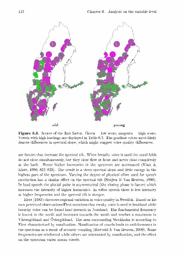
112 Chapter 6. Analysis on the variable level
old young
Figure 6.3. Scores of the �rst factor. Green = low score, magenta = high score.Vowels with high loadings are displayed in Table 6.5. The gradient colors most likelydenote di�erences in spectral slope, which might suggest voice quality di�erences.
are factors that increase the spectral tilt. When breathy voice is used the vocal foldsdo not close simultaneously, but they close �rst at front and never close completelyat the back. Hence higher harmonics in the spectrum are attenuated (Klatt &Klatt, 1990, 822�823). The result is a steep spectral slope and little energy in thehighest part of the spectrum. Varying the degree of physical e�ort used for speechproduction has a similar e�ect on the spectral tilt (Sluijter & Van Heuven, 1996).In loud speech the glottal pulse is asymmetrical (the closing phase is faster) whichincreases the intensity of higher harmonics. In softer speech there is less intensityat higher frequencies and the spectral tilt is steeper.
Elert (1983) discusses regional variation in voice quality in Swedish. Based on hisown perceived observations Elert mentions that creaky voice is used in Småland whilebreathy voice can be found land inwards in Norrland. The fundamental frequencyis lowest in the north and increases towards the south and reaches a maximum inVästergötland and Östergötland. The area surrounding Stockholm is according toElert characterized by nasalization. Nasalization of vowels leads to anti-formants inthe spectrum as a result of acoustic coupling (Rietveld & Van Heuven, 2009). Somefrequencies are reinforced while others are attenuated by nasalization, and the e�ecton the spectrum varies across vowels.

6.3. Co-occurring vowel features 113
The conclusion that the �rst factor of this study is connected to voice qualitydi�erences is only speculative and has not been con�rmed by other analyses of thedata. Regional di�erences in voice quality should be studied further with instru-mental methods. Possible explanations for the low PC2 values in Svealand andFinland are more use of breathy voice or the use of less vocal e�ort (that is, softerspeech) than in Götaland and Norrland, or nasal voice quality.
6.3.3 Factor 2
The second factor correlates with the long close vowels in typ, dis, sot and lus(Table 6.6). This concerns the onset value and degree of diphthongization of PC1 ofthe vowels in typ, dis and lus and PC2 of the sot vowel. The factor explains 9.1%of the total variance.
The maps in Figure 6.4 show that the South Swedish varieties clearly di�er fromthe rest on this factor. These varieties have a clear magenta color, which means highscores and indicates higher PC1 values at the onset in the vowels in typ, dis and lusand higher PC2 values in the vowel in sot than in the rest of the language area. Thissuggests a more open pronunciation at onset in typ, dis and lus and a more frontedpronunciation at onset in sot.
The loadings related to the degree of diphthongization of these vowels are alsopositive, which suggests higher diphthongization values for the South Swedish vari-eties than for the other varieties. As explained in � 6.3.1, positive diphthongizationvalues indicate decreasing PC scores during the vowel segment, while negative diph-thongization values indicate increasing PC scores. A diphthongization value close tozero means a monophthong-like pronunciation. Because the diphthongization valuescan be both positive and negative, the range of the diphthongization values of theobjects has to be taken into account when interpreting factor scores connected todiphthongization. The box plots in Figure 6.5 show the dispersion of the variablesmeasuring the amount of diphthongization with high loadings on the second factor.The central box spans values around or slightly above zero for all four variables,which means that most varieties have a monophthong-like pronunciation. All of thefour vowels show a number of outliers with high positive values close to 1, and forthe sot vowel even higher. Since the South Swedish varieties have high positive
Table 6.6. High loadings on the secondfactor (9.1% variance explained).
vowel measure pc loading
typ /y:/ diphth pc1 0.849typ /y:/ onset pc1 0.843dis /i:/ diphth pc1 0.782sot /u:/ onset pc2 0.767dis /i:/ onset pc1 0.755sot /u:/ diphth pc2 0.706lus /0:/ diphth pc1 0.683lus /0:/ onset pc1 0.583
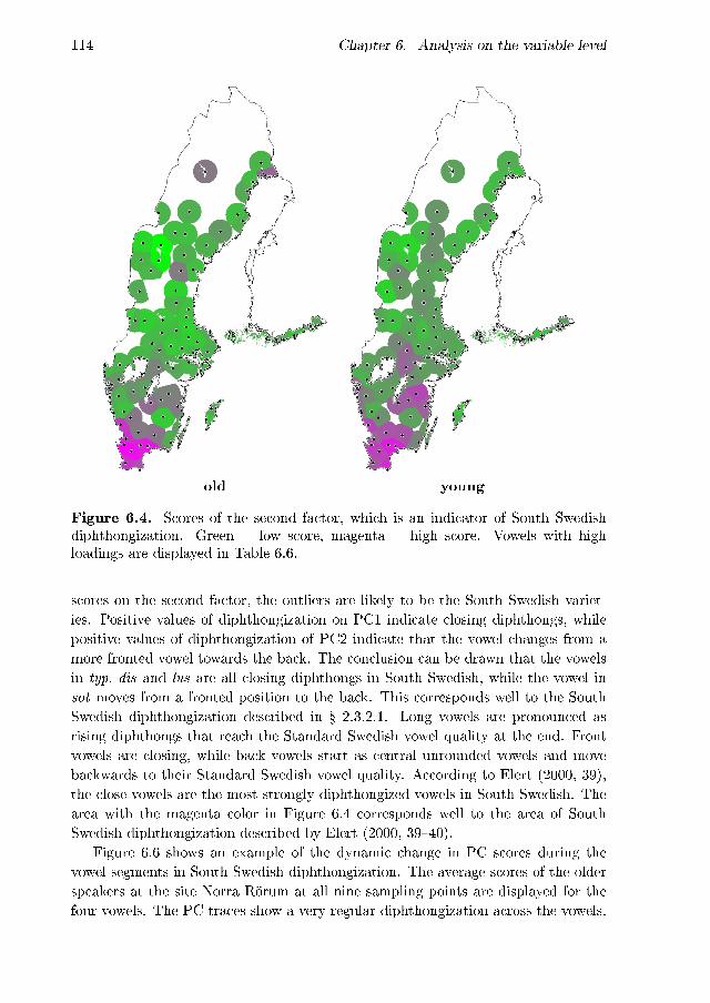
114 Chapter 6. Analysis on the variable level
old young
Figure 6.4. Scores of the second factor, which is an indicator of South Swedishdiphthongization. Green = low score, magenta = high score. Vowels with highloadings are displayed in Table 6.6.
scores on the second factor, the outliers are likely to be the South Swedish variet-ies. Positive values of diphthongization on PC1 indicate closing diphthongs, whilepositive values of diphthongization of PC2 indicate that the vowel changes from amore fronted vowel towards the back. The conclusion can be drawn that the vowelsin typ, dis and lus are all closing diphthongs in South Swedish, while the vowel insot moves from a fronted position to the back. This corresponds well to the SouthSwedish diphthongization described in � 2.3.2.1. Long vowels are pronounced asrising diphthongs that reach the Standard Swedish vowel quality at the end. Frontvowels are closing, while back vowels start as central unrounded vowels and movebackwards to their Standard Swedish vowel quality. According to Elert (2000, 39),the close vowels are the most strongly diphthongized vowels in South Swedish. Thearea with the magenta color in Figure 6.4 corresponds well to the area of SouthSwedish diphthongization described by Elert (2000, 39�40).
Figure 6.6 shows an example of the dynamic change in PC scores during thevowel segments in South Swedish diphthongization. The average scores of the olderspeakers at the site Norra Rörum at all nine sampling points are displayed for thefour vowels. The PC traces show a very regular diphthongization across the vowels.
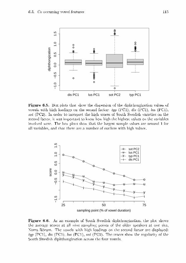
6.3. Co-occurring vowel features 115
●
●●●
●
●
●
●
●●●
●
●
●
●●
●
●
●
●
●
●●●
●
●●
●●●●●
●
●
●
●
●
●
dis PC1 lus PC1 sot PC2 typ PC1
−1.
0−
0.5
0.0
0.5
1.0
1.5
diph
thon
giza
tion
Figure 6.5. Box plots that show the dispersion of the diphthongization values ofvowels with high loadings on the second factor: typ (PC1), dis (PC1), lus (PC1),sot (PC2). In order to interpret the high scores of South Swedish varieties on thesecond factor, it was important to know how high the highest values on the variablesinvolved were. The box plots show that the largest sample values are around 1 forall variables, and that there are a number of outliers with high values.
ii
i ii
i ii i
sampling point (% of vowel duration)
scor
e
25 50 75
−1.
5−
0.5
0.0
0.5
1.0
1.5
yy
yy
yy y y y
uu u
u uu u u u
oo
oo
oo
oo o
ouyi
sot PC2lus PC1typ PC1dis PC1
Figure 6.6. As an example of South Swedish diphthongization, the plot showsthe average scores at all nine sampling points of the older speakers at one site,Norra Rörum. The vowels with high loadings on the second factor are displayed:typ (PC1), dis (PC1), lus (PC1), sot (PC2). The traces show the regularity of theSouth Swedish diphthongization across the four vowels.
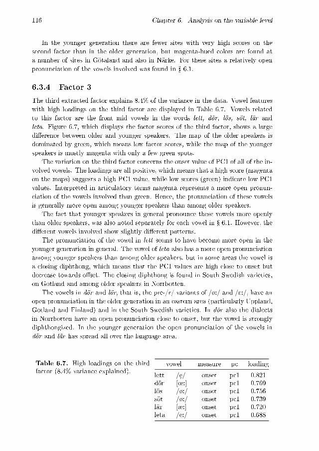
116 Chapter 6. Analysis on the variable level
In the younger generation there are fewer sites with very high scores on thesecond factor than in the older generation, but magenta-hued colors are found ata number of sites in Götaland and also in Närke. For these sites a relatively openpronunciation of the vowels involved was found in � 6.1.
6.3.4 Factor 3
The third extracted factor explains 8.4% of the variance in the data. Vowel featureswith high loadings on the third factor are displayed in Table 6.7. Vowels relatedto this factor are the front mid vowels in the words lett, dör, lös, söt, lär andleta. Figure 6.7, which displays the factor scores of the third factor, shows a largedi�erence between older and younger speakers. The map of the older speakers isdominated by green, which means low factor scores, while the map of the youngerspeakers is mostly magenta with only a few green spots.
The variation on the third factor concerns the onset value of PC1 of all of the in-volved vowels. The loadings are all positive, which means that a high score (magentaon the maps) suggests a high PC1 value, while low scores (green) indicate low PC1values. Interpreted in articulatory terms magenta represents a more open pronun-ciation of the vowels involved than green. Hence, the pronunciation of these vowelsis generally more open among younger speakers than among older speakers.
The fact that younger speakers in general pronounce these vowels more openlythan older speakers, was also noted separately for each vowel in � 6.1. However, thedi�erent vowels involved show slightly di�erent patterns.
The pronunciation of the vowel in lett seems to have become more open in theyounger generation in general. The vowel of leta also has a more open pronunciationamong younger speakers than among older speakers, but in some areas the vowel isa closing diphthong, which means that the PC1 values are high close to onset butdecrease towards o�set. The closing diphthong is found in South Swedish varieties,on Gotland and among older speakers in Norrbotten.
The vowels in dör and lär, that is, the pre-/r/ variants of /ø:/ and /E:/, have anopen pronunciation in the older generation in an eastern area (particularly Uppland,Gotland and Finland) and in the South Swedish varieties. In dör also the dialectsin Norrbotten have an open pronunciation close to onset, but the vowel is stronglydiphthongized. In the younger generation the open pronunciation of the vowels indör and lär has spread all over the language area.
Table 6.7. High loadings on the thirdfactor (8.4% variance explained).
vowel measure pc loading
lett /efl/ onset pc1 0.821dör [œ:] onset pc1 0.769lös /ø:/ onset pc1 0.756söt /ø:/ onset pc1 0.739lär [æ:] onset pc1 0.720leta /e:/ onset pc1 0.688
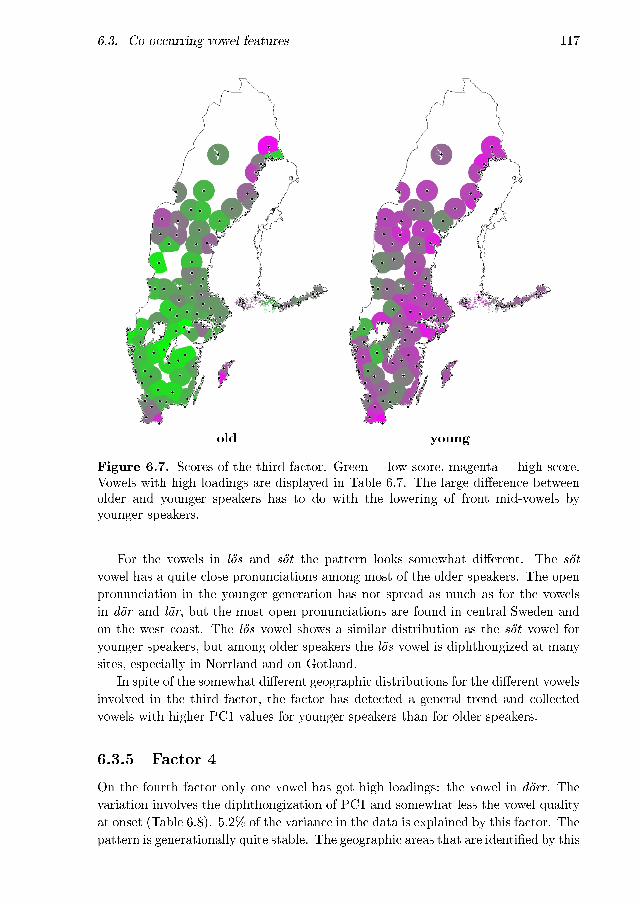
6.3. Co-occurring vowel features 117
old young
Figure 6.7. Scores of the third factor. Green = low score, magenta = high score.Vowels with high loadings are displayed in Table 6.7. The large di�erence betweenolder and younger speakers has to do with the lowering of front mid-vowels byyounger speakers.
For the vowels in lös and söt the pattern looks somewhat di�erent. The sötvowel has a quite close pronunciations among most of the older speakers. The openpronunciation in the younger generation has not spread as much as for the vowelsin dör and lär, but the most open pronunciations are found in central Sweden andon the west coast. The lös vowel shows a similar distribution as the söt vowel foryounger speakers, but among older speakers the lös vowel is diphthongized at manysites, especially in Norrland and on Gotland.
In spite of the somewhat di�erent geographic distributions for the di�erent vowelsinvolved in the third factor, the factor has detected a general trend and collectedvowels with higher PC1 values for younger speakers than for older speakers.
6.3.5 Factor 4
On the fourth factor only one vowel has got high loadings: the vowel in dörr. Thevariation involves the diphthongization of PC1 and somewhat less the vowel qualityat onset (Table 6.8). 5.2% of the variance in the data is explained by this factor. Thepattern is generationally quite stable. The geographic areas that are identi�ed by this

118 Chapter 6. Analysis on the variable level
Table 6.8. High loadings on the fourthfactor (5.2% variance explained).
vowel measure pc loading
dörr [œ] diphth pc1 -0.773dörr [œ] onset pc1 -0.572
old young
Figure 6.8. Scores of the fourth factor, which is connected to the pronunciation ofthe vowel in dörr (see Table 6.8). Green = low score, magenta = high score.
factor are the South Swedish area and the province of Jämtland (Figure 6.8). Theloadings are negative, which suggests that variants with high scores (magenta) havea lower diphthongization value. In � 6.1.14 negative diphthongization values on PC1(that is, an opening diphthong) were found in Jämtland and in the South Swedisharea, while most varieties of Swedish do not have a diphthongized pronunciation. Inthe South Swedish area the vowel starts and ends more open than in Jämtland.
Because only one vowel is involved in the fourth factor, the factor does notcontribute much to the detection of co-occurring features. What the factor tells us,is that varieties with a diphthongized pronunciation of the vowel in dörr also havelow PC1 values close to onset.

6.3. Co-occurring vowel features 119
Table 6.9. High loadings on the �fthfactor (5.2% variance explained).
vowel measure pc loading
sot /u:/ onset pc1 0.813sot /u:/ diphth pc1 0.758lus /0:/ diphth pc2 0.571
old young
Figure 6.9. Scores of the �fth factor. Green = low score, magenta = high score.The underlying factor is secondary diphthongization of the vowels in sot and lus onGotland and in Norrbotten (Table 6.9).
6.3.6 Factor 5
The �fth factor identi�es two very clear dialect groups: the dialects of Gotland andthe dialects in Norrbotten (Figure 6.9). However, on Gotland both older and youngerspeakers are assigned high scores (magenta), while in Norrbotten the younger speak-ers have low scores like the rest of the language area. The variation involves the onsetvalue and diphthongization of PC1 of the vowel in sot and to some extent the diph-thongization of the vowel in lus (Table 6.9). The �fth factor explains 5.2% of thevariance in the data.
Diphthongization of these two vowels on Gotland and among older speakers inNorrbotten was also detected in �� 6.1.7 and 6.1.19. The type of diphthongizationof the vowel in lus was found to vary across the dialects in Norrbotten.

120 Chapter 6. Analysis on the variable level
On Gotland, diphthongization of these vowels (so-called secondary diphthongiz-ation, see � 2.3.3) is part not only of the local dialects, but also of standard-likespeech (see � 2.3.2). On the basis of only this factor no conclusions can, thus, bedrawn about whether the Gotlandic speakers speak a traditional dialect or a moreleveled standard-like variety.
In Norrbotten diphthongs are characterizing for the traditional dialects. How-ever, in standard-like speech in this area diphthongs are lacking (Johansson, 1982;Elert, 1994). According to Figure 6.9, most of the younger speakers in Norrbottendo not use diphthongs. This feature seems to be leveled and the pronunciation ofthe vowels is closer to Standard Swedish.
6.3.7 Factor 6
The amount of variance explained by the sixth factor is 4.9%. The vowels withhigh loadings are the vowels in the words lott, lat and lass (Table 6.10). Thesevowels have changed very little between the older and younger generation accordingto the results in the previous section (Table 6.2, p. 105). Also in Figure 6.10, whichdisplays the scores of the sixth factor, the geographic variation pattern looks very
old young
Figure 6.10. The sixth factor identi�ed small, geographically conditioned di�er-ences in the pronunciation of the vowels in lott, lat and lass (see Table 6.10). Green= low score, magenta = high score.

6.3. Co-occurring vowel features 121
similar in the older and younger generation. All of these vowels also show a relativelysmall amount geographic variation (Table 6.1, p. 103). Apparently, the sixth factorcatches relatively subtle di�erences.
The variation concerns the amount of diphthongization of PC2. For the vowelin lott the loading is excellent, while the vowels of lat and lass have lower loadings.The loadings are positive, which indicates that variants with higher scores (magenta)have higher diphthongization value.
Mainly South Swedish varieties and a number of varieties in Norrland are assignedlow scores (green) on this factor. Also the older speakers of some sites in Svealandand on Gotland have low scores, as well as some of the Finland-Swedish varieties.The highest scores are found in Götaland. Di�erences in the diphthongization of thevowel in lott between varieties Götaland and Norrland were also noted in � 6.1.18.
Table 6.10. High loadings on the sixthfactor (4.9% variance explained).
vowel measure pc loading
lott /O/ diphth pc2 0.732lat /A:/ diphth pc2 0.635lass /a/ diphth pc2 0.568
6.3.8 Factor 7
The amount of diphthongization on PC1 of the vowel in the words lås/låt, nät andlär correlates positively with the seventh factor (Table 6.11), which explains 4.7%of the variance in the data.
The amount of diphthongization of PC1 of lås/låt and nät both have a meanvalue close to 0 and a standard deviation of 0.3. Low scores (green), hence, indic-ate negative diphthongization values, while high scores (magenta) suggest positivediphthongization values. The vowel in lär has less variation in the degree of diph-thongization, with a mean of −0.1 and a standard deviation of 0.2.
Figure 6.11 shows that the dialects on Gotland have the lowest scores in theolder generation, together with some Central Swedish varieties. The low scoressuggest opening diphthongs in lås/låt and nät. This is a part of the Gotlandicdiphthongization described in � 2.3.2.3.
Eklund & Traunmüller (1997) noted a substantial diphthongization of mid vowelsin Standard Swedish, which could �t with the green Central Swedish area in themaps.
Table 6.11. High loadings on the sev-enth factor (4.7% variance explained).
vowel measure pc loading
lås/låt /o:/ diphth pc1 0.797nät /E:/ diphth pc1 0.751lär [æ:] diphth pc1 0.571

122 Chapter 6. Analysis on the variable level
old young
Figure 6.11. Scores of the seventh factor, which is primarily determined by theamount of diphthongization of the vowels in lås/låt and nät (see Table 6.11). Green= low score, magenta = high score.
High scores (magenta) suggest closing diphthongs in lås/låt and nät, while inter-mediate colors indicate a more monophthong-like pronunciation. Conclusions aboutthe pronunciation in lär are harder to draw because of the lower correlation.
In the younger generation the geographic distribution on the seventh factor looksvery similar to the older generation, but there are less extreme scores overall.
6.3.9 Factor 8
The eighth factor explains 3.7% of the total variance. As Figure 6.12 shows, thereis one extreme outlier on the eighth factor. That is the older speakers in Överkalix(Norrbotten). Two vowels have high loadings: the vowels in lass and lat (Table 6.12).The pronunciation of these vowels in Överkalix is discussed in � 6.1.
Apart from the one outlier, low scores are found for example in the South Swedisharea and in Uppland, while Västergötland has very high scores.

6.3. Co-occurring vowel features 123
Table 6.12. High loadings on theeighth factor (3.7% variance explained).
vowel measure pc loading
lass /a/ onset pc1 0.714lat /A:/ onset pc1 0.652
old young
Figure 6.12. Scores of the eighth factor, connected to the pronunciation of thevowels in lass and lat. Green = low score, magenta = high score.
6.3.10 Factor 9
On the ninth factor not a single variable attained a loading that could be consideredgood. The highest loading was the one of the onset value of PC2 of the vowel ofthe word dör, which was 0.504. Nonetheless, 3.1% of the variance in the data isexplained by this factor, and some geographic areas can be identi�ed in the maps inFigure 6.13.
In the older generation the dialects of Jämtland have very high scores (magenta),while east Svealand is assigned the lowest scores together with sites on the Finnishsouth coast. In the younger generation, the varieties are not assigned as extremescores as in the older generation. The east Svealand dialects are more similar to thesurrounding area in the younger generation than in the older generation. In Finland,low scores are maintained in the younger generation. The dialects of Norrbotten arevery di�erent from each other in the older generation, but the younger speakers inthis area are assigned very similar scores.

124 Chapter 6. Analysis on the variable level
old young
Figure 6.13. Scores of the ninth factor. Green = low score, magenta = high score.No variables obtained loadings ≥ 0.55
6.3.11 Factor 10
On the tenth factor only one variable has a good correlation: the amount of diph-thongization on PC2 of the vowel in lös (0.577). The amount of variance explainedis 2.9%. In Figure 6.14, the most extreme low scores (green) on this factor are foundon Gotland and the most extreme high scores (magenta) are found in Kalix andNederlulå (Norrland). Dialects in both these areas are known to have preservedProto-Nordic diphthongs, like the one in lös (see � 2.3.3). Still, the pronunciationin these two areas is di�erent according to the factor scores. The diphthongizationon PC2 in Kalix and Nederluleå is mentioned in � 6.1.12. For the Gotlandic vari-eties, no large di�erence between the vowels in söt and lös was found in � 6.1, butdiphthongization of Standard Swedish /ø:/ was detected on Gotland.
In Gotland the scores on the tenth factor are similar in the older and youngergeneration. In Norrbotten there has been a dramatic change between the two gen-erations.

6.4. Summary 125
old young
Figure 6.14. Scores of the tenth factor. Green = low score, magenta = high score.Vowel with high loading: lös.
6.4 Summary
In this chapter the geographic variation and age related variation in the 19 di�erentvowels in the data set were analyzed. A detailed view of the variation in each vowelwas given in � 6.1, while the amount of geographic and age related variation acrossthe 19 vowels was compared quantitatively in � 6.2. In a factor analysis (FA, � 6.3),the variance in the data set was reduced into ten underlying factors. The threedi�erent methods applied in this chapter supplement each other. The quantitativecomparison in � 6.2 and the FA in � 6.3 detect vowels and variables which showsimilar kinds of variation and, hence, summarize the data. The analysis per vowel in� 6.1 gives a detailed account for the variation beyond the comprehensive patternsdetected by the two other analyses.
The comparison of the amount of variation on the 19 di�erent vowels, in � 6.2,showed that long vowels vary more than short vowels both across sites and across thetwo age groups. The two geographically most varying vowels in both age groups werethe vowels in dör (Standard Swedish [œ:]) and sot /u:/, while the geographicallyleast varying vowels were the vowels in disk /I/, lass /a/ and särk [æ]. Almost allvowels vary geographically less in the younger speaker group than in the older. Theaverage linguistic distance between dialects is signi�cantly shorter in the younger
126 Chapter 6. Analysis on the variable level
speaker group than in the older speaker group. The linguistic distances becomingshorter indicates an ongoing dialect leveling in the Swedish language area. Thevowels with the most decrease in geographic variation were the vowels in lär [æ:]and lat /A:/. Only the vowel in söt /ø:/ showed considerably more geographicvariation among younger speakers than in the older age group.
Some of the factors in the FA identi�ed distinct dialect groups in the data, whileothers showed a more continuous distribution of the vowel features. Some dialectareas were identi�ed by a number of the extracted factors. For example, the �rstand the ninth factor showed a relationship between dialects in Svealand and thedialects along the Finnish south coast. The dialects on Gotland were shown byseveral factors to share some vowel features that distinguish them from the otherSwedish dialects (factors three, �ve, seven and ten). The second factor showed thatthe most distinguishing feature of South Swedish is the diphthongization of long closevowels. A number of factors also identi�ed distinguishing features for the dialects inNorrland. Especially in the provinces Jämtland (factors three, four and nine) andNorrbotten (factors three, �ve and ten) divergent dialects are found among the olderspeakers.
Factors seven and nine showed similar geographical distribution patterns in theolder and younger generation of speakers, but among the younger speakers the factorscores were less extreme. These factors might either show that a lower number ofthe younger speakers than of the older use the dialectal features (that is, some ofthe younger speakers at a site use the standard variant and others the local variantwhich gives less extreme average values than for older speakers), or that the dialectalmarkers are maintained by younger speakers but the acoustic distances between thevariants are becoming smaller.
Some factors failed to bundle together features of several vowels, but only cor-related highly with one of the vowels in the data set. For example, factor four onlycorrelated highly with the vowel in the word dörr and showed that the vowel qualityclose to the onset of this vowel is connected to the amount of diphthongization.
The eighth factor identi�ed one outlier in the data set. It showed the olderspeakers in Överkalix have a divergent pronunciation of the vowels in lass and lat.
The sixth factor showed that the vowels in lott, lat and lass co-occur when itcomes to the amount of diphthongization. However, the analyses in �� 6.1 and 6.2showed that the total amount of variation in these vowels is very small.
The Swedish front mid vowels showed most variation across the two age groups.The vowels in the words lär [æ:], nät /E:/, lös /ø:/, dör [œ:], lett /efl/, söt /ø:/ andleta /e:/ were found to have the largest average distances between older and youngerspeakers in � 6.2. All of these vowels, except for the vowel in nät, were also found toco-occur by the third factor of the FA. This suggests that the change in the vowelin nät has a di�erent distribution than that in the other vowels. The FA showedthat what these vowels have in common is that the PC1 values are higher amongyounger speakers than among older speakers, which means that the pronunciationis becoming more open. The results in � 6.1 showed that the vowels in lär, nät andlett are becoming more open in almost the whole Swedish language area. For the

6.4. Summary 127
vowel in dör a more close pronunciation is preserved only in western parts, while theopening of the vowel in lös and söt is restricted to a smaller area in central Swedenand on the west coast.
The change towards a more open pronunciation of the vowels in lär and dör,means a change in the direction of the standard language and varieties spoken aroundStockholm. In the case of nät, however, the varieties around Stockholm (togetherwith other eastern varieties) have the most close pronunciation in the older gener-ation and the varieties around Stockholm are the ones that are changing the most.The close pronunciation of the nät vowel in Stockholm (due to a merger of /e:/ and/E:/) has never been accepted as Standard Swedish (Elert, 2000, 47).
The spreading of a more open pronunciation of the vowels in söt and lös (Stand-ard Swedish /ø:/) is described by Nordberg (1975) as a change from below (see� 6.1.11). The open variant has previously been stigmatized and used mainly byspeakers in the lower social classes. In Nordberg's study, however, open variantswere more common among younger speakers than among older speakers, and wereused also by higher social class youth. In an FA of a number of dialectal featuresin the spoken language of Eskilstuna, Hammermo (1989) showed that there was aco-variation between /ø:/ and /E:/. The open pronunciation of these vowels was in-terpreted by Hammermo as a marker of local identi�cation with Eskilstuna. Otherfeatures that co-varied to some extent with these vowels were the pronunciationof /0:/ and the degree of Central Swedish diphthongization (� 2.3.2.2). In Ham-mermo's data young girls used more open variants of /ø:/ and /E:/ than young boys.Aniansson (1996) analyzed the same data as Hammermo (1989) and made the inter-pretation that the open variants were not seen as local markers by the girls, but hadbecome the more prestigious pronunciation. A similar trend was shown by Kotsinas(1994), who described the di�usion of the previously stigmatized open pronunciationof these vowels to Stockholm, where girls, not least in the upper-class, exceeded boysin the use of open variants.
The impact of the lowering of /ø:/ and /E:/ on a large part of the languagearea is shown very clearly in the analyses in this chapter. Also for the speakerswho represent Standard Swedish this ongoing change could be noted. The formerlystigmatized variants, hence, seem to be becoming the preferred variants. Milroy,Milroy, & Hartley (1994) described a case where female speakers starting to use apreviously stigmatized feature (glottalization) in British English led to the featuregaining prestige. They suggested that women create prestige instead of being theones adapting the most to the standard language, which has been postulated inmany other studies. This hypothesis �ts very well with the Swedish data. In thestudies by Hammermo (1989), Kotsinas (1994) and Aniansson (1996), young girlswere the ones favoring previously stigmatized open pronunciations of /ø:/ and /E:/.Comparison of older and younger speakers in the present study shows the di�usionof the open pronunciation to a large number of rural Swedish sites, and even tospeakers considered representatives of Standard Swedish.


Chapter 7
Aggregate analysis
The previous chapter showed that groups can be identi�ed among Swedish dialectsbased on some speci�c vowel features. Contrary to analyzing separate features,the dialectometric research tradition has emphasized the aggregate analysis whichshows how dialects relate to each other when all available variables are consideredsimultaneously (Nerbonne, 2009). Common aggregating methods are cluster analysisand multidimensional scaling (MDS). Both methods use a distance matrix with thepairwise distances between all objects as input. MDS is a method for reducingcomplex distance data to interpretable low-dimensional representations, while clusteranalysis produces partitions of the data. MDS is suitable for visualizing dialectcontinua, while cluster analysis detects dialect groups.
Cluster analysis is a relatively unstable method where small di�erences in theinput data can result in substantially di�erent outputs (Jain & Dubes, 1988; Ner-bonne, Kleiweg, Heeringa, & Manni, 2008). In an analysis of Bulgarian dialectsProki¢ & Nerbonne (2008) found that only clusters that could be visually identi�edin a two-dimensional MDS plot were identi�ed with high con�dence by a number ofclustering algorithms. Legendre & Legendre (1998, 482) argue that when only twoor three dimensions are considered in MDS the analysis might fail to identify par-titions that are distinguished in higher dimensions. However, when applying MDSto dialect data three dimensions generally explain at least around 90% of the totalvariance in the data (Heeringa, 2004; Proki¢ & Nerbonne, 2008). Hence, higherdimensions are unlikely to play any role in identifying group structure.
Tibshirani, Walter, & Hastie (2001) proposed a method called Gap statistic forestimating the number of groups in a data set. The Gap statistic can be used forestimating the number of signi�cant clusters produced by any clustering algorithm.Lundberg (2005) used the Gap statistic to estimate the number of signi�cant clusterswhen grouping the Swedish dialects based on acoustic analysis of the vowel in theword lat (/A:/ in Standard Swedish) and found three signi�cant clusters.
129

130 Chapter 7. Aggregate analysis
The Gap statistic was applied to the present data set using the CLUTO1 software.The analysis showed that there are no well separated clusters in the data set. Thisresult suggests that the Swedish dialects form a true continuum when it comesto an aggregate analysis of vowel pronunciation. The absence of clearly separabledialect groups is in agreement with previous research. The dialects in the Swedishlanguage area are said to form a true continuum without abrupt borders (see � 2.2.1).Clustering methods could be applied to the data, but they are likely to produceunstable results, since any sharp division into subsets is not in agreement with thestructure of the data. In this chapter, an aggregate analysis of vowel pronunciationin Swedish dialects is proposed by means of MDS. The MDS plots (for example,Figure 7.1) con�rm the view that the Swedish language area is a genuine dialectcontinuum.
In � 7.1 MDS is described, and � 7.2 gives the results of a number of MDSanalyses. The results of the aggregate analyses are summarized in � 7.3.
7.1 Multidimensional scaling
Multidimensional scaling (MDS) reduces complex distance data to low-dimensionalrepresentations and allows visualization of the distances in a low-dimensional space.Like principal component analysis (PCA, � 5.1.2) and factor analysis (FA, � 6.3.1)MDS is a dimensionality reduction technique. One di�erence between PCA andFA, on one hand, and MDS, on the other, is that PCA and FA analyze the full datamatrix where every object is described by a number of variables, while MDS analyzesthe distances/similarities between objects based on some chosen distance/similaritymeasure. In MDS the aim is to represent the objects in a small number of dimensions,while the exact preservation of original distances is less important than in PCA orFA (Legendre & Legendre, 1998, 444). In MDS priority is given to preserving theordering of the objects instead of the exact distances between objects. Becauseof this, MDS allows us to investigate the relationships between dialects in fewerdimensions than FA. MDS is normally used to scale to two or three dimensions,since more dimensions are di�cult to visualize simultaneously.
The results of MDS presented below show that MDS scaled to three dimensionsexplains more than 95% of the variance in the present data set. This can be comparedto the FA in the previous chapter, where ten factors explained only 60.6% of the totalvariance in the data. However, FA explains 60.6% of the variance in the originaldata, while MDS explains 95% of the variance in the distance matrix. Convertingthe original data to pairwise aggregate distances as such reduces the amount ofinformation in the data. The FA showed how Swedish dialects relate to each otherwhen some speci�c features are considered. By reducing the data to a smallernumber of dimensions than FA, MDS gives an aggregate analysis, that is, it allows
1CLUTO: software for clustering high-dimensional data sets. By the De-partment of Computer Science and Engineering, University of Minnesota.<http://glaros.dtc.umn.edu/gkhome/views/cluto>

7.2. Dialect continuum 131
us to see how the dialects relate to each other when all variables are taken intoaccount simultaneously.
In MDS, original distances between objects are approximated in a low-dimen-sional space by an iterative algorithm (Jain & Dubes, 1988). A number of algorithmsfor MDS have been proposed. In a study of the linguistic distances between varietiesof Dutch Heeringa (2004) measured the �tness of three di�erent MDS proceduresby correlating the original distances with the Euclidean MDS coordinate-based dis-tances, and found that Kruskal's non-metric MDS gave the best results. In thischapter Kruskal's non-metric MDS, as implemented in the RuG/L042 software, isbeing used.
For the MDS the distances between the varieties were calculated as the averagedistance of the 19 vowels in the data set. First, the distance for each vowel betweentwo varieties was calculated as the Euclidean distance of the acoustic variables ofvowel quality (Equation 6.1, p. 102), that is, two principal components (PCs), meas-ured at nine di�erent points within each vowel segment, starting at 25% of the totalvowel duration and ending at 75%. Subsequently, the average of the vowel distanceswas calculated. At some locations not all of the 19 vowels were elicited and thosesites had to be left out from the FA (� 6.3). However, the average vowel distancebetween two objects can be calculated also for a fewer number of vowels withoutbiasing the ordering of the data. Therefore, sites and speaker groups that were leftout from the FA could be included in the MDS.
Results from MDS are often visualized in two- or three-dimensional coordinatesystems. In this representation similar items are found close to each other, whiledissimilar items are far apart. Nerbonne, Heeringa, & Kleiweg (1999) proposed amethod for displaying the results of MDS of dialect data on maps. Each of thethree basic colors in the RGB color model is used to represent one dimension ofthe MDS (see Appendix B, � B.1). Hence, each position in the three-dimensionalspace will be represented by a unique color (Figure B.1, p. 211). On the maps, thearea of each variety is colored with the color corresponding to the position in thethree-dimensional space. In this way, the positions in the MDS space are connectedto the geographic locations, and the colors in the maps show how similar or distantdialects are to each other in a three-dimensional linguistic space.
7.2 Dialect continuum
In order to explore the Swedish dialect continuum, MDS was applied to three di�er-ent divisions of the data. In � 7.2.1 the geographic variation is described by averagingover all speakers per site. In � 7.2.2 the data is split into older and younger speakersper site. Since this division of the data is the same as the one that was used in theFA in � 6.3, a comparison with the results of the FA allowed for an interpretation
2RuG/L04: software for dialectometrics and cartography. By P. Kleiweg, University of Gro-ningen. <http://www.let.rug.nl/kleiweg/L04/>

132 Chapter 7. Aggregate analysis
of the MDS dimensions, which is reported in � 7.2.3. In � 7.2.4 a further divisionaccording to gender is made.
Group means were calculated for PC1 and PC2 respectively for each of the 19vowels at the nine sampling points (see the lowest part of Figure 5.12 on p. 72).Subsequently the Euclidean distances between varieties were calculated based onthe group means, and the resulting distances matrix was analyzed with MDS.
7.2.1 Geographic variation
In the �rst MDS analysis, average values for each site (that is, the averages ofthe approximately twelve speakers) were calculated for the acoustic variables beforemeasuring the linguistic distances between sites and applying MDS. The distancematrix comprised the pairwise distances between all 98 sites.
Figure 7.1 shows the results of the MDS in a two-dimensional coordinate systemwhere the gray-scale color of the dot represents the third dimension. One dimensionexplains 81.4% of the variance, two dimensions 93.6% and three dimensions 96.3%.It is clear that the �rst dimension already explains a very large part of the variance.Using more than three dimensions would only mean a small improvement of thevariance explained. The plot does not show any clear clusters of sites, but there is
Ankarsrum
Anundsjö
Arjeplog Asby
Aspås
Bara
BengtsforsBerg
Bjurholm
Borgå
Bredsätra
Broby
Brändö
Burseryd
BurträskBöda
Dalby
Delsbo
Dragsfjärd
Fjällsjö
Floby
Fole
Frillesås
Frostviken
Frändefors
Färila
Fårö
Gräsö
Gåsborn
Hammarö
Hamneda
Haraker
Houtskär
HusbyIndal
Jämshög
Järnboås
Järsnäs
Kalix
Korsberga
Kramfors
Kyrkslätt
Kärna Kårsta
Leksand
Lillhärdal
Länna
Löderup
Malung
Nederluleå
Nora
Norra Rörum
Nysätra
Närpes
Ockelbo
Orust
Ovanåker
Piteå
Ragunda
Rimforsa
S:t Anna
Saltvik
Segerstad
Skee
Skinnskatteberg
Skog
Skuttunge
SnappertunaSorunda
Sproge
Stenberga
Stora Mellösa
Storsjö
Strömsund
Särna
Södra Finnskoga
Torhamn
Torp
Torsås
Torsö
Vemdalen
Viby
Vilhelmina
VillbergaVindeln
VäckelsångVästra Vingåker
Våxtorp
Vörå
Åre
Årstad−Heberg
Årsunda
Össjö
Östad
Överkalix
Öxabäck
Figure 7.1. Results of MDS to three dimensions of linguistic distances betweensites. The �rst dimension is represented by the x-axis, the second dimension by they-axis and the third dimension by the gray-scale color of the dot. Because of thedensity of sites close to the origin, a few labels have been omitted.
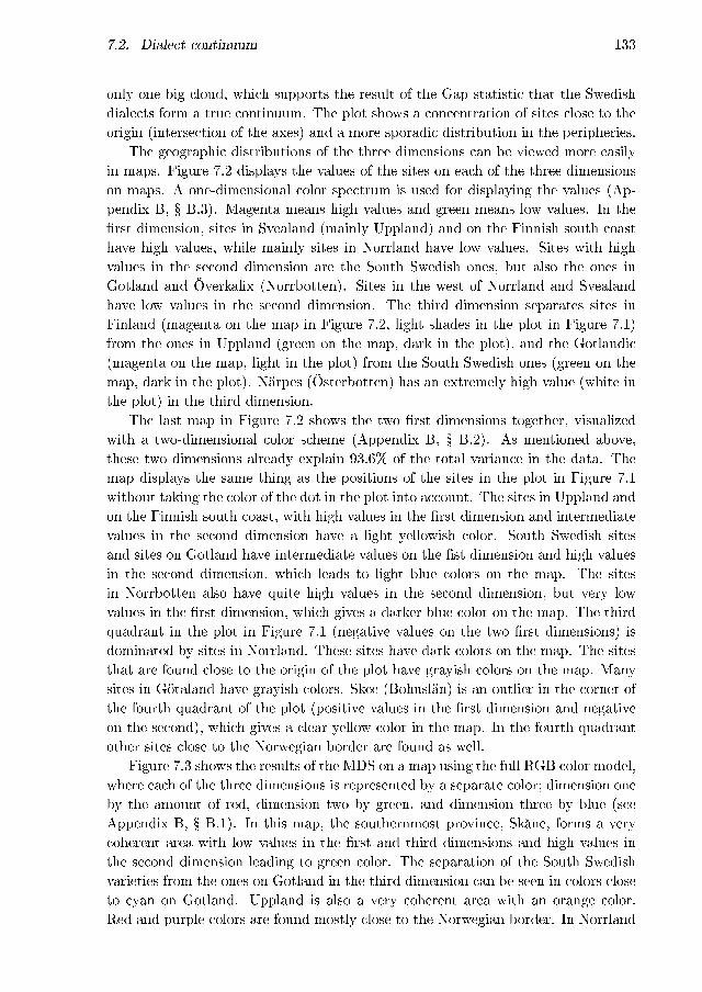
7.2. Dialect continuum 133
only one big cloud, which supports the result of the Gap statistic that the Swedishdialects form a true continuum. The plot shows a concentration of sites close to theorigin (intersection of the axes) and a more sporadic distribution in the peripheries.
The geographic distributions of the three dimensions can be viewed more easilyin maps. Figure 7.2 displays the values of the sites on each of the three dimensionson maps. A one-dimensional color spectrum is used for displaying the values (Ap-pendix B, � B.3). Magenta means high values and green means low values. In the�rst dimension, sites in Svealand (mainly Uppland) and on the Finnish south coasthave high values, while mainly sites in Norrland have low values. Sites with highvalues in the second dimension are the South Swedish ones, but also the ones inGotland and Överkalix (Norrbotten). Sites in the west of Norrland and Svealandhave low values in the second dimension. The third dimension separates sites inFinland (magenta on the map in Figure 7.2, light shades in the plot in Figure 7.1)from the ones in Uppland (green on the map, dark in the plot), and the Gotlandic(magenta on the map, light in the plot) from the South Swedish ones (green on themap, dark in the plot). Närpes (Österbotten) has an extremely high value (white inthe plot) in the third dimension.
The last map in Figure 7.2 shows the two �rst dimensions together, visualizedwith a two-dimensional color scheme (Appendix B, � B.2). As mentioned above,these two dimensions already explain 93.6% of the total variance in the data. Themap displays the same thing as the positions of the sites in the plot in Figure 7.1without taking the color of the dot in the plot into account. The sites in Uppland andon the Finnish south coast, with high values in the �rst dimension and intermediatevalues in the second dimension have a light yellowish color. South Swedish sitesand sites on Gotland have intermediate values on the �st dimension and high valuesin the second dimension, which leads to light blue colors on the map. The sitesin Norrbotten also have quite high values in the second dimension, but very lowvalues in the �rst dimension, which gives a darker blue color on the map. The thirdquadrant in the plot in Figure 7.1 (negative values on the two �rst dimensions) isdominated by sites in Norrland. These sites have dark colors on the map. The sitesthat are found close to the origin of the plot have grayish colors on the map. Manysites in Götaland have grayish colors. Skee (Bohuslän) is an outlier in the corner ofthe fourth quadrant of the plot (positive values in the �rst dimension and negativeon the second), which gives a clear yellow color in the map. In the fourth quadrantother sites close to the Norwegian border are found as well.
Figure 7.3 shows the results of the MDS on a map using the full RGB color model,where each of the three dimensions is represented by a separate color; dimension oneby the amount of red, dimension two by green, and dimension three by blue (seeAppendix B, � B.1). In this map, the southernmost province, Skåne, forms a verycoherent area with low values in the �rst and third dimensions and high values inthe second dimension leading to green color. The separation of the South Swedishvarieties from the ones on Gotland in the third dimension can be seen in colors closeto cyan on Gotland. Uppland is also a very coherent area with an orange color.Red and purple colors are found mostly close to the Norwegian border. In Norrland

134 Chapter 7. Aggregate analysis
dim 1 dim 2
dim 3 dim 1�2
Figure 7.2. Results of MDS to three dimensions of linguistic distances betweensites. All three dimensions visualized separately, green = low values, magenta =high values. The two �rst dimensions are also visualized together in the lower rightmap.
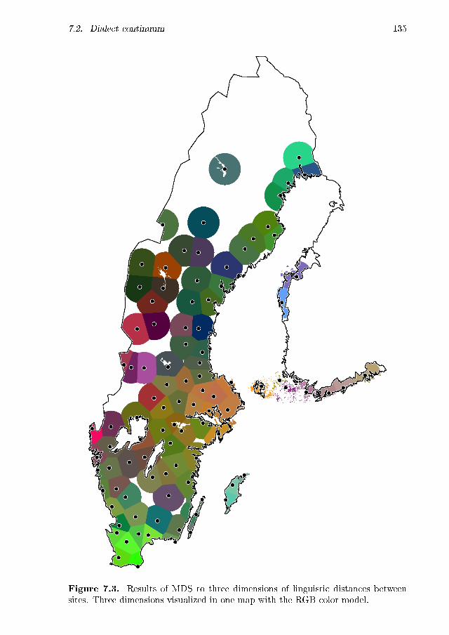
7.2. Dialect continuum 135
Figure 7.3. Results of MDS to three dimensions of linguistic distances betweensites. Three dimensions visualized in one map with the RGB color model.

136 Chapter 7. Aggregate analysis
mostly dark green colors are found, but also other dark colors and blue. Götalandis quite incoherent with di�erent colors from the center of the color spectrum. InFinland there is a clear di�erence between the sites on the south coast and thewest coast. Saltvik (Åland) is much more similar to the sites in Uppland than toFinland-Swedish varieties.
The map where all three dimensions are represented shows that even if the dis-tribution of dialectal features is continuous, some more coherent dialect areas canbe detected.
7.2.2 Analysis based on age
In the following step age-related variation was analyzed in addition to the geographicvariation. The distance matrix that MDS was applied to comprised the pairwiselinguistic distances between 196 objects (2 age groups × 98 sites). One dimensionexplains 78.9% of the variance, two dimensions 92.3% and three dimensions 95.9%.
Figure 7.4 shows the results of the MDS in a two-dimensional coordinate systemwhere the gray-scale color of the dot represents the third dimensions. The objects
O
Y
O
YO
Y
O
Y
O
Y
O
Y
O
Y
O
Y
O
YO
Y
O
Y
O
Y
O
Y
O
Y
O
Y
O
Y
O
Y
O
Y
O
Y
O
Y
O
Y
O
Y
O
Y
O
Y
O
Y
O
Y
O
Y
O
Y
O
Y
O
Y
O
Y
O
Y
O
Y
O
YO
Y
O
Y
O
Y
O
Y
O
Y
O
Y
O
Y
O
Y
O
Y
O
Y
O
Y
O
Y
O
Y
O
YO
Y
O
Y
O
Y
O
Y O
Y
O
Y
O
Y
O
Y
O
Y
O
Y
O
Y
O
Y
O
Y
O
Y
O
Y
O
Y
O
Y
O
Y
O
Y
O
Y
OYO
Y
O
Y
O
Y
O
Y
O
Y
O
Y
O
Y
O
Y
O
Y
O
Y
OYO
Y
O
Y
O
Y
O
Y
O
Y
O
Y
O
Y
O
Y
O
Y
O
Y
O
Y
O
Y
O
Y
O
Y
O
Y
O
Y
O
Y
O
Y
Figure 7.4. Results of MDS to three dimensions of linguistic distances betweensites and age groups. The �rst dimension is represented by the x-axis, the seconddimension by the y-axis and the third dimension by the color of the dot. O = olderspeakers, Y = younger speakers.

7.2. Dialect continuum 137
old young
Figure 7.5. The �rst dimension of MDS of linguistic distances between sites andage groups. Green = low values, magenta = high values.
form one big cloud, except for one outlier, which for some reason has an extremelyhigh value in the second dimension. This outlier is the younger speakers of Löderup(Skåne). The labels of the objects do not �t into the plot, but for each object a letterindicates whether the dot concerns older or younger speakers. As can be seen, thesecond dimension mainly seems to separate the two age groups. The older speakersmostly have low values in the second dimension, while younger speakers have highvalues.
For getting a better picture of the distribution of the values in each dimensionone-dimensional maps were created. Figure 7.5 shows the values in the �rst di-mension of the older and younger speakers of each site. The extremely high valueof the younger speakers of Löderup in the second dimension would mean that alarge proportion of the color representing the second dimension would be requiredfor representing this variety. In order to produce more separation between the othervarieties the young speakers of Löderup were left out of the color visualizations. Themaps show that in this analysis sites in Svealand and on the Finnish south coast areassigned low values in the �rst dimension while sites in Norrland have high valuesin the �rst dimension. This is roughly the reverse of the analysis per site in theprevious section. However, in MDS the directions of the axes are arbitrary and may

138 Chapter 7. Aggregate analysis
old young
Figure 7.6. The second dimension of MDS of linguistic distances between sites andage groups. Green = low values, magenta = high values.
be rotated (Legendre & Legendre, 1998, 445), which means that the �rst dimensionin both analyses roughly represents the same thing. The maps of older and youngerspeakers look quite similar.
As already shown by the scatter plot in Figure 7.4, the second dimension mainlyseparates older and younger speakers. The maps of the second dimension in Fig-ure 7.6 con�rm the picture of the scatter plot. However, for some of the peripheraldialects (South Swedish, Gotland, Finland, Norrland) there is not such a large dif-ference between older and younger speakers in the second dimension.
Figure 7.7 shows that high values in the third dimension are assigned to SouthSwedish sites, Gotlandic and all of the Finland-Swedish sites except for Åland. Theolder speakers in Norrbotten have high values, while young speakers in Norrbottenhave low values in the third dimension. The lowest values in the third dimensionare found in Jämtland. The third dimension could, hence, be interpreted as a peri-pherality dimension.
The maps in Figure 7.8 display all three dimensions of the MDS of older andyounger speakers per site simultaneously using the whole three-dimensional RGBcolor spectrum. The two age groups are displayed on separate maps, but the colorsof the two maps are comparable since they are based on one single MDS analysis
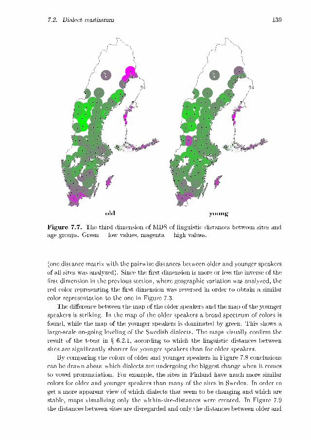
7.2. Dialect continuum 139
old young
Figure 7.7. The third dimension of MDS of linguistic distances between sites andage groups. Green = low values, magenta = high values.
(one distance matrix with the pairwise distances between older and younger speakersof all sites was analyzed). Since the �rst dimension is more or less the inverse of the�rst dimension in the previous section, where geographic variation was analyzed, thered color representing the �rst dimension was reversed in order to obtain a similarcolor representation to the one in Figure 7.3.
The di�erence between the map of the older speakers and the map of the youngerspeakers is striking. In the map of the older speakers a broad spectrum of colors isfound, while the map of the younger speakers is dominated by green. This shows alarge-scale on-going leveling of the Swedish dialects. The maps visually con�rm theresult of the t-test in � 6.2.1, according to which the linguistic distances betweensites are signi�cantly shorter for younger speakers than for older speakers.
By comparing the colors of older and younger speakers in Figure 7.8 conclusionscan be drawn about which dialects are undergoing the biggest change when it comesto vowel pronunciation. For example, the sites in Finland have much more similarcolors for older and younger speakers than many of the sites in Sweden. In order toget a more apparent view of which dialects that seem to be changing and which arestable, maps visualizing only the within-site-distances were created. In Figure 7.9the distances between sites are disregarded and only the distances between older and

140 Chapter 7. Aggregate analysis
old young
Figure 7.8. MDS to three dimensions of linguistic distances between sites andage groups. Both age groups were included in one single MDS analysis, and arerepresented within the same color spectrum making the colors of the two mapscomparable with each other.
younger speakers at each site are displayed. The map to the left shows the distancesvisualized with a continuous one-dimensional color spectrum (Appendix B, � B.3).The sites with the shortest aggregate distance between older and younger speakersare green, while sites with a large distance between older and younger speakers aremagenta.
For getting an even more distinct picture, the sites were divided into three groupsusing K-means clustering.3 The map to the right in Figure 7.9 shows three groupsobtained by clustering sites with the most similar distances between the two agegroups. When three distinct groups are formed, all sites with only a relativelysmall distance between older and younger speakers are clear green, sites with a largedistance are magenta, and all sites with intermediate distances between older andyounger speakers are pure gray.
Dialects in the South Swedish area, on the islands Öland and Gotland, and inFinland are green, and hence have small average distances in vowel pronunciation
3K-means is the most commonly used clustering algorithm for partitioning data. The userdecides how many groups should be formed, and the algorithm partitions the most similar itemsinto groups by minimizing the total error sum of squares (Legendre & Legendre, 1998, 349�355).
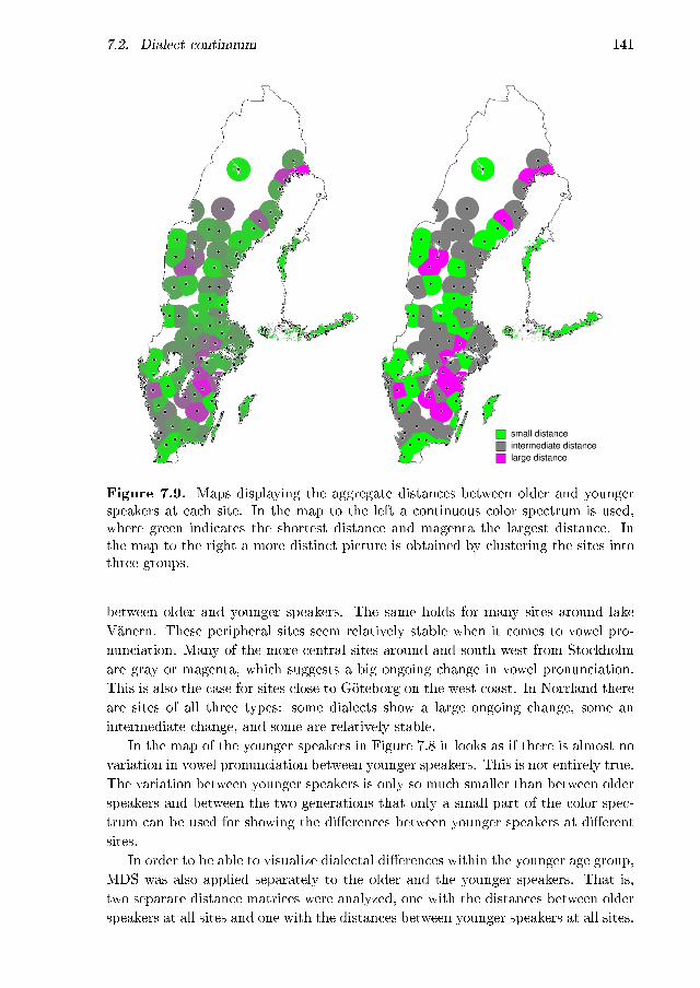
7.2. Dialect continuum 141
Figure 7.9. Maps displaying the aggregate distances between older and youngerspeakers at each site. In the map to the left a continuous color spectrum is used,where green indicates the shortest distance and magenta the largest distance. Inthe map to the right a more distinct picture is obtained by clustering the sites intothree groups.
between older and younger speakers. The same holds for many sites around lakeVänern. These peripheral sites seem relatively stable when it comes to vowel pro-nunciation. Many of the more central sites around and south-west from Stockholmare gray or magenta, which suggests a big ongoing change in vowel pronunciation.This is also the case for sites close to Göteborg on the west coast. In Norrland thereare sites of all three types: some dialects show a large ongoing change, some anintermediate change, and some are relatively stable.
In the map of the younger speakers in Figure 7.8 it looks as if there is almost novariation in vowel pronunciation between younger speakers. This is not entirely true.The variation between younger speakers is only so much smaller than between olderspeakers and between the two generations that only a small part of the color spec-trum can be used for showing the di�erences between younger speakers at di�erentsites.
In order to be able to visualize dialectal di�erences within the younger age group,MDS was also applied separately to the older and the younger speakers. That is,two separate distance matrices were analyzed, one with the distances between olderspeakers at all sites and one with the distances between younger speakers at all sites.

142 Chapter 7. Aggregate analysis
old young
Figure 7.10. MDS to three dimensions of linguistic distances between sites for eachage group separately. The maps are based on two separate MDS analyses, so thatthe full color spectrum is used in each of the maps. The colors are not comparableacross the two maps.
The analysis of only older speakers included 98 sites and the amount of explainedvariance was 82.1% for the �rst dimension, 93.4% for two dimensions and 95.7% forthree dimensions. The analysis of only younger speakers included 97 sites (youngerspeakers in Löderup were left out) and the amount of explained variance was 83.8%for the �rst dimension, 92.4% for two dimensions and 96.1% for three dimensions.
Figure 7.10 shows the maps with results of MDS applied separately to the olderand younger speakers. Since two separate analyses are displayed in the two maps, thecolors of the maps have to be interpreted independently.4 The maps are similar tothe ones in Figure 7.8, but the colors in each map are more distinct. When the wholecolor spectrum is used for each age group separately it becomes clear that there aredi�erences across sites among the younger speakers, which could not be distinguishedin Figure 7.8. Moreover, the geographic pattern is quite similar for older and youngerspeakers. So even if the dialectal di�erences in vowel pronunciation are larger in the
4For example, Gotland has completely di�erent color in the two maps. This does not mean thatthere is a large di�erence in vowel pronunciation between older and younger speakers on Gotland,it is only an e�ect of the full color spectrum being used to visualize the distances within each agegroup.

7.2. Dialect continuum 143
older generation than in the younger, the geographic distribution of dialectal featuresremains more or less the same.
Some di�erences in the geographic distributions can also be found. For example,the dialects in Norrland are more coherent in the younger age group than in the older.Figure 7.9 showed that some dialects in Norrland are relatively stable, while othershave a large linguistic distance between older and younger speakers. In Norrland themost divergent dialects seem to be changing the most, and thereby a more uniformspoken variety of Norrland is emerging. This can be seen as regionalization of thedialects, since the most divergent dialectal features seem to be disappearing whilesome other features that distinguish Norrland varieties from other Swedish varietiesare preserved.
7.2.3 Interpreting MDS dimensions
Because MDS is based on a distance matrix with pairwise aggregate distancesbetween varieties, MDS does not o�er any direct way to interpret which of theoriginal linguistic variables that have caused the distribution in the extracted di-mensions. In factor analysis (FA), however, the loadings indicate the correlationbetween original variables and extracted factors. In � 6.3 the average acoustic val-ues per age group per site were analyzed by means of FA. The same division of thedata into older and younger speakers per site was used in the MDS in � 7.2.2, whichmakes a comparison between MDS and FA possible.
The values of the objects in the three dimensions of the MDS were correlatedwith the scores of the FA using Pearson's correlation. The correlations are displayedin Table 7.1. The �rst dimension corresponds well to the �rst factor (r = 0.921) andthe second dimension correlates highly with the third factor (r = 0.840). The thirddimension does not show very high correlations with one single factor, but seemsto be a combination of several of the factors. Most strongly the third dimensioncorrelates with the �fth (r = 0.468) and the ninth (r = −0.502) factor.
Since the FA includes loadings that tells us which of the linguistic variables areconnected to each factor, a linguistic interpretation of the MDS dimensions can beinferred from the correlations with the factors. Based on the loadings of the FA, the
Table 7.1. Pearson's correlationsbetween factors and MDS dimensions.Insigni�cant correlations (p > 0.05) areindicated by a dash.
dim1 dim2 dim3
factor1 0.921 −0.227 �factor2 0.213 0.302 0.313factor3 0.224 0.840 �factor4 � � 0.195factor5 � � 0.468factor6 � � �factor7 � −0.160 0.176factor8 � 0.177 −0.320factor9 � −0.162 −0.502factor10 � � −0.218

144 Chapter 7. Aggregate analysis
conclusion can be drawn that the �rst dimension of the MDS is largely based ondi�erences in the PC2 values of front vowels (compare with the loadings of the �rstfactor of the FA in Table 6.5, p. 111), which is assumed to be connected to voicequality di�erences.
The second dimension of the MDS correlates highly with the third factor of theFA, and hence has to do with di�erences in the PC1 values of front mid vowels(Table 6.7, p. 116). The FA showed that these vowels are lowered by youngerspeakers in many areas.
The third dimension is more unspeci�c and shows the e�ect of several variables,which have di�erent geographic distribution patterns according to the FA. It seemsthat varieties with extreme scores in the third dimension of the MDS are not neces-sarily linguistically very similar to each other, but they are characterized by dialectalfeatures that make them divergent from more central varieties.
The e�ect of the second factor of the FA, which distinguishes South Swedishvarieties from the rest, is spread over all three dimensions of the MDS (signi�cantcorrelations between 0.2 and 0.3 with all three dimensions).
The sixth factor of the FA, which detected only very subtle di�erences betweendialects (see � 6.3.7), does not correlate signi�cantly with any of the MDS dimensions.
7.2.4 Analysis according to age and gender
In the �nal MDS analysis the data from every site were divided into four groups:older men, older women, younger men, younger women. This resulted in a 390 ×390 distance matrix (speaker groups with less than 15 vowels were not included, seeAppendix A). One dimension explains 82.5% of the variance, two dimensions 93.0%and three dimensions 95.9%.
Figures 7.11�7.13 display one-dimensional maps of the three �rst dimensionsseparately, with one map for each speaker group. Green color indicates low valuesand magenta high values (see Appendix B, � B.3).
The solution is similar to the one in � 7.2.2, only with the second and third dimen-sions reversed. Low values in the �rst dimension (Figure 7.11) were assigned mainlyto Svealand and the Finnish south coast, even though the geographic distribution isnot completely coherent.
The second dimension (Figure 7.12) mainly separates older and younger speakers.At most sites, the younger speakers have low values, while high values are foundamong older speakers (the inverse of the second dimension of the MDS in � 7.2.2).In the second dimension the older women have somewhat higher values on averagethan the older men.
As in the analysis in � 7.2.2, the third dimension (Figure 7.13) could be called aperipherality dimension. South Swedish, Gotlandic and Finland-Swedish sites andthe older speakers in Norrbotten have low values, while speakers in Jämtland havehigh values (the inverse of the third dimension of the MDS in � 7.2.2).
Figure 7.14 displays the four maps that combine all three dimensions using theRGB color model. All three colors were reversed to obtain a color representation

7.3. Conclusions of the aggregate analysis 145
similar to the ones in the previous sections (Figure 7.8 and Figure 7.3). From thesemaps, it is obvious that the di�erences in vowel pronunciation are larger betweenthe two generations than between men and women. The map of the older womenis darker than the one of the older men, mainly due to the second dimension. Asin the analysis in � 7.2.2, we can see that the dialectal di�erences are smaller in theyounger generation than in the older, disregarding the variation across genders. Themaps of both the younger men and the younger women are dominated by green,while the maps of the older speakers show a broader color spectrum. The maps ofthe older speakers show roughly the same geographic patterns that were detected inthe two previous sections, while the color spectrum used for the younger speakersis so narrow that almost no geographic patterns can be detected. For the site Skee(Bohuslän) it can be noted that the younger men have a red color, like older speakers,while the young women have a color much more similar to the surrounding dialects.
7.3 Conclusions of the aggregate analysis
In this chapter the relationships between varieties of Swedish were analyzed using ag-gregate linguistic distances based on acoustic measurements of 19 vowels. The Gapstatistic showed that the data cannot be partitioned into groups, but the Swedishdialects form a continuum without abrupt borders. This is in line with previous de-scriptions of the Swedish dialects. For visualizing the continuum-like relationshipsbetween varieties of Swedish, multidimensional scaling (MDS) was used. Five di�er-ent analyses were carried out using MDS. In � 7.2.1 the linguistic distances betweensites were analyzed. In � 7.2.2 the data were divided into older and younger speakersper site and three analyses were made: one including both older and younger speak-ers, one with only older speakers, and one with only younger speakers. In � 7.2.4 afurther division according to gender was made and an analysis which included fourspeaker groups per site was carried out.
The analysis of linguistic distances between sites showed that even if the distri-bution of dialectal features is continuous, some more coherent dialect areas can bedetected.
The analysis of the two age groups in the data set showed that the dialectaldi�erences are considerably smaller in the younger generation than among olderspeakers. The e�ect of dialect leveling in apparent time is large. However, thegeographic distribution of dialectal features is not changing much, so that the maindialect areas remain the same. This can be interpreted as regionalization of thedialects, since it seems that dialectal features that are characterizing the largerdialect regions are still being preserved at the same time as the overall linguisticdistances become smaller.
An analysis of the distances between the two age groups within each site showedthat the central dialects, close to the biggest cities, seem to be changing the most,while many of the more peripheral dialects are relatively stable when it comes toan aggregate analysis of vowel pronunciation. This can seem surprising, because

146 Chapter 7. Aggregate analysis
in a dialect leveling situation you might expect that the most divergent peripheraldialects would be converging to more central and standard-like varieties. In order tounderstand why the central dialects are changing the most this result of the aggregateanalysis has to be studied in relation to the change in each of the variables. This isdiscussed further in � 8.2.2.
A further division according to gender showed that the di�erences between olderand younger speakers is much larger than the di�erence between men and women.In the older generation there seems to be more gender-related di�erences than inthe younger generation.
The results obtained by MDS could be correlated with results from the factoranalysis (FA) in the previous chapter. This showed that the �rst dimension, whichseparates Svealand and south Finland-Swedish varieties in all the MDS analyses, islargely explained by the PC2 values of front vowels. The second dimension, the oneproducing the largest distance between older and younger speakers, is mainly ane�ect of the lowering of front mid vowels by younger speakers. The third dimensionof the MDS is a peripherality dimension separating peripheral areas in the Swedishlanguage area, like Skåne, Gotland, Finland, Norrbotten and Jämtland. Variablescharacterizing peripheral dialects were spread on several factors with di�erent geo-graphical distributions in the FA.
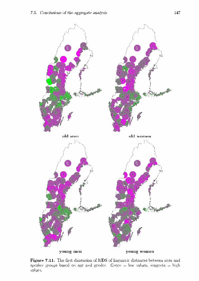
7.3. Conclusions of the aggregate analysis 147
old men old women
young men young women
Figure 7.11. The �rst dimension of MDS of linguistic distances between sites andspeaker groups based on age and gender. Green = low values, magenta = highvalues.

148 Chapter 7. Aggregate analysis
old men old women
young men young women
Figure 7.12. The second dimension of MDS of linguistic distances between sitesand speaker groups based on age and gender. Green = low values, magenta = highvalues.
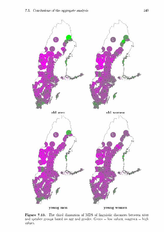
7.3. Conclusions of the aggregate analysis 149
old men old women
young men young women
Figure 7.13. The third dimension of MDS of linguistic distances between sitesand speaker groups based on age and gender. Green = low values, magenta = highvalues.

150 Chapter 7. Aggregate analysis
old men old women
young men young women
Figure 7.14. Results of MDS to three dimensions of linguistic distances betweensites and speaker groups based on age and gender, visualized with the RGB colormodel. All speaker groups are represented within the same color spectrum makingthe colors of the maps comparable with each other.

Chapter 8
Discussion
Below, the results from the three previous chapters are discussed and related toeach other. In � 8.1 the acoustic method is evaluated. In � 8.2 the dialectologicalconclusions about Swedish dialects that can be drawn taking both the analysis onthe variable level and the aggregate level into account are discussed. Finally, in� 8.3, the strengths and limitations of analysis of variables and aggregate analysisare discussed.
8.1 Acoustic analysis
The most common method used in variationist linguistics for assessing vowel qualityacoustically has been formant measurements. In this study another approach waschosen. Vowel spectra were �ltered with Bark �lters up to 18 Bark and subsequentlythe �lter bank representation was reduced to articulatory meaningful principal com-ponents (PCs) by means of principal component analysis (PCA). The method haspreviously been used for large-scale analysis of geographic and social variation inDutch vowel pronunciation by Jacobi (2009).
Bark �lters correspond to the auditory �lters of human hearing, which meansthat a Bark �lter representation of vowels models human perception. Formants, onthe other hand, are resonant frequencies in the vocal tract and measuring formantshence is an articulatory model. A strong association between the two models wasshown by high correlations between PCs and formants in � 5.2.1. The correlationbetween the second component (PC2) and F2 was, however, somewhat weaker thanthe one between the �rst component (PC1) and F1.
Bark �ltering can be automated more reliably than formant measurements. Auto-mated formant measurements always include wrong values that have to be correctedmanually. In addition to the perception-based merits of a �lter bank representation,the load of manual work was reduced signi�cantly by the choice of method for acous-tic analysis. Nonetheless, one should bear in mind that a considerable amount ofmanual work was needed, too, to make this study possible. Preceding the acoustic
151

152 Chapter 8. Discussion
analysis, all the vowel data had been manually segmented in the SweDia project.How to reduce the e�ect of speaker-dependent variation is a problem for all stud-
ies dealing with acoustic speech samples (see �� 2.4.3 and 2.4.4). Due to anatom-ical/physiological di�erences, the overall size of the vowel space varies signi�cantlyacross speakers. A number of normalization procedures have been developed forformant measurements, but none of them work well when one wants to comparevowels from varieties that are not phonologically comparable. Jacobi (2009) solvedthe problem by relating the measurements of each vowel to the speakers point vow-els /i/ and /a/. Jacobi studied the variation in Dutch diphthongs and long vowels.Relative measures of vowel quality could be used because the Dutch point vowelsare considered to be stable across all varieties of Standard Dutch.
Among the Swedish vowels, stable point vowels could not be found for all speak-ers, which excluded the possibility to use a relative measure of vowel quality. Instead,speaker-dependent variation was evened out by averaging over a number of speakersper variety. However, the number of male and female speakers was not equal foreach variety, which meant that the systematic di�erences in the vowel spaces of maleand female speakers due to anatomical/physiological di�erences had to be removedin order not to bias the results. A normalization of the di�erences between male andfemale voices was obtained by applying PCA separately to vowels produced by menand women. This procedure e�ectively removed di�erences in PC scores betweenmen and women (� 5.1.5). Of the point vowels only [u:] showed a signi�cant dif-ference on one of the two extracted PCs after applying PCA separately to men andwomen. Before normalization, that is, when including vowels produced by men andwomen in one single PCA, all four point vowels ([i:], [æ:], [A:]/[a:] and [u:]) showedsigni�cant di�erences between men and women in one or two of the extracted PCs.This possibility to normalize for the e�ect of speaker-sex in the PCs, somethingwhich has been notoriously di�cult in formant measurements, turned out to be abig advantage of the acoustic method chosen.
Using a so-called whole-spectrum method undoubtedly includes more informa-tion from the acoustic signal than only cues directly related to the articulation ofvowels. The signal-to-noise ratio in the recordings has been shown to in�uence PCsextracted from band-pass �ltered spectra both in the present study (dialect speakersrecorded in their homes vs. speakers of Standard Swedish in a studio, see � 5.1.6)and by Jacobi (2009, 59�63). When using this method one should therefore eitherpay attention to all recordings being made in as similar conditions as possible, oralternatively �nd some stable point vowels which can be used for normalizing forthe e�ect of noise.
Regional di�erences were detected in the PCs that did not seem to be connectedto formants and vowel articulation. This spectral feature was connected to PC2of all front vowels and an assumption is that voice quality di�erences would havecaused this regional variation in the PCs. The exact nature of the spectral featureconnected to PC2 of front vowels could, however, not be veri�ed in this study, butshould be studied further. A factor analysis applied to the data seemed to be ableto separate this spectral feature from other variation in the data (� 6.3.2).

8.2. Dialectological results 153
In the analyses of dialectal variation, average values of the PCs for each varietywere used. For example, in the analysis of pure geographic variation, average valueswere computed for each site (that is, average PCs of twelve speakers for most of thesites). In a number of analyses social variation was accounted for as well. When thedata was split up into two age groups the groups on average included six speakers,while a further division according to gender led to even smaller groups (on averagethree speakers per gender per age group per site). Since all speaker-dependentvariation could not be removed from the acoustic PCs, the in�uence of individualdi�erences in the overall size of the vowel space on the group averages is greaterthe smaller the group is. Especially in the division into four groups per site (olderwomen, older men, younger women, younger men), where each group included onaverage only three speakers, some caution should be taken when interpreting theresults. Still, also this division into the smallest groups showed very similar resultsto the other analyses. Most notably the di�erences between the two age groupswas much greater than the di�erences between men and women, with especiallythe younger women and younger men showing very similar results. This can beseen as an additional con�rmation of a successful reduction of di�erences relatedto the anatomical/physiological di�erences between men and women in the acousticmeasure.
The PCs extracted from the Bark-�ltered vowel spectra were used in a numberof analyses of dialectal variation (Chapters 6 and 7). Several features which havepreviously been described in the Swedish dialect literature were identi�ed. Theresults from previous studies could hence be supported by acoustic data and thegeographic distribution of dialectal features across a large number of sites in theSwedish language area could be established. The PCs o�ered an interpretationof the data in terms of vowel height and advancement. A complete articulatorydescription of vowels can, however, not be inferred from the PCs, since for examplevowel roundness is not represented in a simple way in the PCs.
Since using PCA of band-pass �ltered vowel spectra can be automated morereliably than formant measurements, it can be regarded as well-suited for large-scaleanalyses of phonetic variation in vowel quality. Moreover, the method turned outto o�er a possibility to normalize for the systematic di�erence between male andfemale voices, something which has always been regarded as di�cult in formantmeasurements. The perceptual and articulatory correlates of PCs of Bark-�lteredvowel spectra should still be studied further. Especially the variance in PC2, whichwas somewhat less dependent of formants than the variance in PC1, should bestudied in more detail in future research.
8.2 Dialectological results
This section includes a discussion of the dialectological results of Chapters 6 and 7.The dialect areas identi�ed in the aggregate analysis are described linguistically in� 8.2.1 below, and in � 8.2.2 some explanations to the observed language change are

154 Chapter 8. Discussion
discussed. Before going on with the dialectological results some general issues aboutthe representativity of the data should be addressed.
Language change was studied by comparing an older and a younger group ofspeakers at every site. A question to be asked is whether the observed di�erencesbetween speaker groups in apparent time correspond to a real linguistic change. Inthe SweDia project the age range of the younger speakers was chosen so that thelanguage recorded would not be the youth language of teenagers, which is likely tochange when the speakers get older. A somewhat older group comprising speakersin their 20s or early 30s was recorded. Nordberg (2005, 1765) has pointed out thatseveral studies from the Swedish area have shown that �young adults and peoplein early middle age stand out as comparatively more standard-speaking than otherage groups, probably because this is the period of life when careers are built up andthe values of the larger society become important.� On the other hand, Sundgren(2002) studied language change in Eskilstuna with access to language data for bothan apparent time and a real time study. She could conclude that both the study inapparent time and the study in real time showed the same development and thatthe two methods would not lead to di�erent conclusions about ongoing changes.
Another concern would be to what extent the recording situation would in�uencethe dialect speakers and whether older and younger speakers would make di�erentaccommodations to the language of the interviewers. The risk of the speakers beingin�uenced by the speech variety of the interviewers is especially high in sites wherethe speakers are used to switch between or use a gliding scale between the localdialect and Standard Swedish. At some locations the interviews were carried out bya speaker of the local dialect while at other locations the interviewers talked a varietyrepresentative for a larger region. In all cases, the speakers were encouraged to thinkabout how the words would be pronounced in the local vernacular. The impression isthat this strategy was successful in most cases. At some sites, however, the resistanceagainst speaking the local dialect to a stranger was exceptionally strong. This wasperceived to be the case at least for many of the speakers in Snappertuna in Finland.The speakers from this particular site should therefore be regarded as speakers of theregional standard language and not of the local dialect. It cannot be ruled out thatthe dialect speakers have made linguistic accommodations towards the language ofthe interviewers at some other sites, too.
One should keep in mind that the varieties analyzed are a sample of 98 sites fromthe Swedish language area. All possible linguistic variation can therefore not beaccounted for. A few sites which are well known for their well-preserved divergentrural dialects (Orsa and Älvdalen) have been excluded from the current analysis.This is because they were already considered so di�erent from other dialects duringthe SweDia �eldwork that a completely di�erent word list was used for elicitingvowel sounds in these dialects.

8.2. Dialectological results 155
8.2.1 Dialect areas
The results of multidimensional scaling (MDS) to three dimensions in � 7.2.1, whereaverage linguistic distances between sites were analyzed, showed that even if thedistribution of dialectal features is continuous, some more coherent dialect areascan be detected. The map in Figure 7.3 (p. 135) displaying the MDS results isvery similar to the traditional divisions proposed by Wessén (1969) and Elert (1994)(Figure 2.2, p. 14).
Acknowledging the fact that the borders between the Swedish dialect areas arenot abrupt, but form a continuum, Wessén (1969) did not propose any bordersbetween dialect areas, but only gave a rough sketch of a dialect division. This issimilar to what the map displaying the results of MDS shows. There are de�nitelyareas within the Swedish language area which di�er from each other considerablywhen it comes to vowel pronunciation, but between these areas there are no abruptborders, only gradual transitions.
Wessén (1969) classi�ed the Swedish traditional rural dialects, while the clas-si�cation of Elert (1994) was one of regional varieties of Standard Swedish. Theclassi�cation by Wessén (1969) was based on phonetic, phonological and morpho-logical features while Elert (1994) used mainly intonation and di�erences in vowelpronunciation for grouping varieties of the Swedish spoken language. Both scholarsconsidered vowel pronunciation an important characteristic for dialects and regionalvarieties of Swedish. The data of the present study is collected only at rural sites,but the data is about a hundred years younger than the data that Wessén (1969)worked with. Because of the large-scale dialect leveling that has a�ected Swedenduring the last half of the 20th century, traditional rural dialects have been preservedonly in very few areas. The data of this thesis include more dialectal features thanthe varieties in Elert's classi�cation, but more leveled dialects than the ones thatWessén wrote about. The varieties studied in this thesis could be called modernrural varieties of Swedish. The results in � 7.2.2 showed that even if there is consid-erable dialect leveling going on in the Swedish language area, the geographic areasthat can be identi�ed are still very similar for older and younger speakers. Based onthe analysis of the separate vowels in Chapter 6 the areas detected by the aggregateanalysis in Chapter 7 can be described linguistically:
The most prominent feature of South Swedish varieties is the diphthongizationof long vowels. The close long vowels in dis, typ, lus and sot have the strongestdiphthongization, which was identi�ed by the second factor of the factor analysis(FA) in � 6.3. But also the mid vowels in leta, nät, söt, dör and låt are diphthongized,especially in Skåne. The South Swedish varieties have relatively high PC2 values(that is, a more fronted pronunciation than Standard Swedish) in the long and shorta vowels in lat and lass.
In Götaland a more close pronunciation than in Standard Swedish was noted forthe vowels in dör and lär. This is also the case for younger speakers to a greaterextent than in most parts of the language area. The open pronunciation of söt whichis spreading among younger speakers in central Sweden is only found in the coastal
156 Chapter 8. Discussion
areas of Götaland but not land inwards. In many sites in Götaland a more openpronunciation than in Standard Swedish is found for the vowel in lus. Many youngerspeakers also have a relatively open pronunciation in dis and typ. On the west coastand in Dalsland the pronunciation of the disk vowel is more open than elsewhere.In Småland and Östergötland a diphthongization of the vowel in sot can be found.
Svealand is characterized by a spectral feature which distinguishes it from thevarieties in Götaland and Norrland. This spectral feature, identi�ed by the �rstfactor of the FA (� 6.3.2), might be related to voice quality, and should be studiedfurther. Uppland is characterized by a very close pronunciation in nät and anopen pronunciation of the vowels in lär and dör. However, younger speakers inUppland have a more open pronunciation in nät compared to the older speakers.An open pronunciation in söt, which is not common among older speakers, is usedby younger speakers in the whole East Central Swedish area. In Närke a relativelyopen pronunciation of the vowels in dis and typ is found for younger speakers.
Features that are found mainly in sites close to the Norwegian border are an openpronunciation of the vowel in �ytta and for the more northern varieties a frontedpronunciation in lott. A relatively close pronunciation in lär and dör is found forboth older and younger speakers in this area.
In Norrland large linguistic distances between dialects are still found. However,in the most divergent areas, Norrbotten and Jämtland, the younger speakers show aconsiderable convergence to Standard Swedish. Among older speakers in Norrbotten,both Proto-Nordic diphthongs and secondary diphthongs are still found, but mostyounger speakers are not using the diphthongs. For many sites in Norrland a moreopen pronunciation than in Standard Swedish is found in lus and a relatively frontedpronunciation of the a vowels in lat and lass.
The varieties in the southern parts of Finland share a spectral feature (whichmight be connected to voice quality) with dialects in Svealand. In most varietiesin Finland the vowel in lus is a central vowel and not a front vowel as in StandardSwedish. Most sites, but not all, have a relatively close vowel in nät and an openvowel in lär. Proto-Nordic diphthongs are found in Houtskär (Åboland) and inÖsterbotten and secondary diphthongs primarily in Österbotten. A more frontedpronunciation than in Standard Swedish in lat is found especially in the south ofFinland.
Gotland is mainly characterized by the rich number of diphthongs�both Proto-Nordic and secondary diphthongs are found. The pronunciation of the vowels in lärand dör is open, and the vowel in lat is more fronted on Gotland than in StandardSwedish.
Two features which are considered characteristic for the vowel pronunciation ofregional varieties of Swedish were not identi�ed in the analyses in this thesis. Theseare Central Swedish diphthongization (� 2.3.2.2) and the occurrence of a semi-vowelor fricative ending in long close vowels in central Sweden (� 2.3.2.4). The reasonthat these features were not identi�ed in the present data set could have to do withthe choice of sampling points in the vowel segments. The �rst sampling point was at25% of the vowel duration and the last at 75%, so it is possible that diphthongization

8.2. Dialectological results 157
in the very �rst and last part of the vowel segments is missed. However, CentralSwedish diphthongization is considered prosodically conditioned and is strongest instressed vowels and in the end of sentences, while the semi-vowel or fricative endingin vowels is most noticeable in word �nal position and before another vowel. Dueto these facts the two types of diphthongization might not be prominently presentin the data set. The speakers were pronouncing words in isolation, which wouldexclude many prosodic features, and all vowels were in a C C context, which is notfavorable for the semi-vowel or fricative ending.
Comparison with results from other studies where data from the SweDia data-base have also been used, makes it possible to draw conclusions about associationsbetween di�erent linguistic levels. The intonational typology by Bruce (2004) (seethe description in � 2.2.3) largely corresponds to the dialect areas described byWessén (1969) and Elert (1994), and hence also to the areas detected in the presentthesis. The intonational variation and the variation in vowel pronunciation seem tohave very similar geographic distributions.
Schae�er (2005) made a typology of phonological quantity in Swedish dialects,also using SweDia data. The three main types identi�ed by Schae�er form ratherdi�erent geographic areas than the ones identi�ed based on vowel pronunciation. InSchae�er's study, Sweden was divided into a southern and a northern area with theborder between the two areas approximately following the border between Svealandand Norrland. A transitional dialect border between Svealand and Norrland can besupported by the aggregate analysis in the present study. However, the di�erencesbetween and within Svealand and Götaland are too large for grouping the dialectsin these areas into one class based on vowel pronunciation. The third type identi�edby Schae�er comprised the mainland Finland-Swedish varieties, which clearly forma separate group also in the present study. The dialects on Åland belong to thenorthern type in Schae�er's study. The present thesis also shows that the varietieson Åland share more vowel features with varieties in Sweden than with the Finland-Swedish dialects, but in contrast to Schae�er's results, Åland is more similar toUppland than to the dialects in Norrland when it comes to vowel pronunciation.
Hopefully more analyses of additional linguistic levels will be carried out in thefuture using data from the SweDia database. Quantitative comparisons of data fromdi�erent linguistic levels could show interesting interactions and form the basis forlinguistic typologies.
8.2.2 Change and leveling
The comparisons of the vowel pronunciation of older and younger speakers in thisthesis (� 6.2.2 and � 7.2.2) suggest large-scale dialect leveling; the linguistic distancesbetween sites are shorter for younger speakers than for older speakers. The aggregateanalysis revealed that the sites that show the largest amount of change are many ofthe most central ones close to the biggest cities, while many of the peripheral dialectareas, which are most divergent from Standard Swedish, are relatively stable whenit comes to vowel pronunciation.

158 Chapter 8. Discussion
The aggregate analysis as such does not provide an explanation for why thecentral dialects are changing the most. In order to �nd an answer, the variation andchange on the variable level has to be studied. The analysis in � 6.2.2 showed thatthe vowels responsible for the largest amount of change are the vowels in the wordslär, nät, lös, dör, lett and söt. The analysis of each of the vowels in � 6.1 showedthat the patterns of change look quite di�erent for some of these vowels.
Even though one neutral variety of Standard Swedish hardly exists, there are stillvariants that are more or less associated with a Standard Swedish pronunciation.An example is the open pronunciation of the phonemes /E:/ and /ø:/ before /r/,which is associated with Central Standard Swedish pronunciation (Bruce, 2010, 118,Grönberg, 2004, 139). The open variants of /E:/ and /ø:/, that is [æ:] and [œ:], wereelicited with the words lär and dör in the present study. The analyses showed thatolder speakers in large parts of Sweden have a much more close pronunciation thanthe Standard Swedish one. An open pronunciation corresponding to the StandardSwedish one is found among older speakers mainly in eastern parts of the languagearea, for example in the surroundings of Stockholm where the open pronunciationof these vowels has been a part of the rural dialects. Among younger speakers theopen pronunciation has become much more widespread, so for these two vowels thereseems to be a clear case of convergence to Standard Swedish.
For the vowel in nät the pattern of change is di�erent. The traditional pro-nunciation in Stockholm and the surrounding dialects has been [e:], while the pro-nunciation generally accepted as Standard Swedish and the pronunciation in mostdialectal varieties of Swedish is [E:]. The Stockholm pronunciation is the result of amerger of the phonemes /e:/ and /E:/, which has never been accepted as StandardSwedish (Elert, 2000, 46). However, the merger is not a complete one, since in frontof /r/ the two vowels are kept apart also in Stockholm and surrounding dialects.1
For the nät vowel the present data set shows that older speakers around Stockholmhave a much more close pronunciation than most other varieties of Swedish (exceptfrom varieties on Gotland and in Finland). In the younger generation the sites closeto Stockholm have a more open pronunciation than in the older generation. Forthe nät vowel, there is a change towards Standard Swedish, but the sites that arechanging the most and giving way for the Standard Swedish pronunciation are theones closest to Stockholm. At the same time the pronunciation of the nät vowelalso seems to be becoming even more open in many parts of the language area,approaching [æ:].
For the vowels in söt and lös yet another geographic pattern of change is found.In both these words the Standard Swedish vowel phoneme is /ø:/.2 The data showsthat while the older speakers at most sites have a relatively close pronunciationof the söt vowel, younger speakers in a large east central area have a more openpronunciation. A change towards a more open vowel is also found on the west
1There is a distinction between /le:ra/ [le:ra] `clay' and /lE:ra/ [læ:ra] `learn', but not between/le:ka/ [le:ka] `play' and /lE:ka/ [le:ka] `heal'.
2Some dialects have preserved a Proto-Nordic diphthong in lös, and in these dialects the wordssöt and lös have di�erent vowel phonemes.

8.2. Dialectological results 159
coast and even among the speakers who represent Standard Swedish in the SweDiadatabase.
The vowel in lett, for which a large degree of change was noted in � 6.2.2, too,seems to show a similar change in the whole language area. At almost all sites inthe data set the pronunciation is more open among younger speakers than amongolder speakers.
In summary, the vowels in lär, dör and nät all show convergence to StandardSwedish. The dialect area surrounding Stockholm has traditionally had a standard-like pronunciation of lär and dör and therefore does not show much change in thesetwo vowels. In nät the dialects close to Stockholm have a more close pronunciationthan the standard pronunciation among older speakers, but young speakers seem toconverge towards the Standard Swedish pronunciation. At the same time a change isfound in the vowels in nät, söt and lett, which cannot be seen as a convergence to thestandard language but it is a relatively new feature in Swedish. These vowels have amore open pronunciation among younger speakers than among older speakers. Thevowels in nät and lett seem to become more open in the Swedish dialects in general.For the vowel in söt (for most varieties of Swedish equal to the vowel in lös) thechange towards a more open pronunciation is strongest in central Sweden and onthe west coast, while some more peripheral areas are less a�ected by the change.
There is hence a complex situation lying behind the maps in Figure 7.9 (Chapter 7,p. 141), which show that dialects in central Sweden and on the west coast are theones that are changing the most, while several peripheral dialects seem more stable.Convergence to the standard language partly explains the change, but the di�usionof a new more open pronunciation of some of the front vowels among young speak-ers, which is not a change towards what traditionally has been considered StandardSwedish, also explains a large part of the change.
The lowering of /E:/ and /ø:/ has been noted by scholars before. Especially thelocal vernacular of Eskilstuna has been the subject to many studies, and the loweringof /E:/ and /ø:/ in Eskilstuna has been described by Nordberg (1975), Hammermo(1989) and Aniansson (1996). Kotsinas (1994) has described the use of the moreopen variants of these vowels among teenagers in Stockholm, and Andersson (1994)noted the spread of an open /ø:/ in Göteborg. Grönberg (2004) considered the openvariant of /ø:/ as a marker of general Swedish youth language and particularly ofthe vernaculars of the cities. In Grönberg's study of teenagers in Västergötland thefrequency of open /ø:/ was generally low, but the frequency grew higher the closerthe subjects lived to Göteborg, which indicated di�usion from the city.
8.2.2.1 Diachronic view
In � 6.1.11, Nordberg's (1975) explanation for the emergence of a more open pro-nunciation of /ø:/ in Eskilstuna was described. Initially it was a �socio-linguistichypercorrection� that occurred among lower-class speakers when the speakers, whoin their own dialect only had a close variant of /ø:/, wanted to imitate the moreopen pronunciation [œ:] used before /r/ in Standard Swedish. The hypercorrection

160 Chapter 8. Discussion
Table 8.1. Older Swedish vowel system with ten long vowels.front central back
−round +roundclose i y 0 umid e ø oopen E œ a
Table 8.2. The Swedish long vowel system after /œ:/ had merged with /o:/.front central back
−round +roundclose i y 0 umid e ø oopen E a
occurred when the dialect speakers did not restrict themselves to using the openvariant only before /r/ but in all contexts. In a second stage of the change, the openpronunciation in other than pre-/r/ context di�used to speakers of all social-classesin a change from below (Nordberg, 1975), and some decades later entered Stockholmyouth language (Kotsinas, 1994).
Nordberg (1975) goes one step further back in the language history in order toexplain the development of the more open pronunciation of /ø:/. Until the mid18th century Swedish had ten long vowel phonemes, which formed the symmetricalphonological system in Table 8.1. There was a separate phoneme /œ:/ which in themiddle of the 18th century merged with /o:/. The disappearance of the phoneme/œ:/ left a hole in the phonological system, as can be seen in Table 8.2.
The hole left in the Swedish long vowel system by the disappearance of /œ:/was �lled by the emergence of a more open allophone of /ø:/, which had untilthen been one uniform sound without any allophones in complementary distribution(Nordberg, 1975). In the latter half of the 18th century /ø:/ was lowered before /r/in the spoken language of the higher social classes in Central Sweden. A similarallophonic variation is found for /E:/ (/E:/ → [æ:] / /r/). To �t in the pre-/r/variants of both /ø:/ and /E:/ in the vowel system a fourth degree of vowel heightis needed for front vowels.
The Standard Swedish vowel system with nine long vowels and pre-/r/ variantsof /ø:/ and /E:/ has been di�cult to describe phonologically, as already explainedin � 2.3.1. One reason for this is that sometime during the 19th century /0:/ lostits central position in Table 8.1 and became a phonetically front vowel, which madethe close front part of the vowel system very crowded. Articulatory and acoustically/0:/ was distinguished from /y:/ and /ø:/ by another type of rounding; /0:/ hasbeen described as in-rounded while /y:/ and /ø:/ are out-rounded. Constructinga simple symmetric phonological system with distinctive features was impossibletaking phonetic facts and phonological variations into account. Table 8.3 shows twoexamples of distinctive features for Swedish long vowels that have been proposed.
In many Swedish dialects the phoneme /œ:/ was preserved much longer than

8.2. Dialectological results 161
Table 8.3. Two examples of the numerous di�erent structural descriptions of theSwedish long vowels that have been proposed (allophonic variants are not included).
Malmberg (1956): Traunmüller & Öhrström (2007):front back front back
round0 round1 round2 round0 round1 round2
close i y u i y 0 umid e ø 0 o e ø oopen E a E a
Table 8.4. Long vowel system in Eskilstuna (Nordberg, 1975).front back
−round +roundclose i y umid e 0 oopen E ø a
in the standard language. In these dialects there was no room for a lowering of/ø:/ before /r/, because /œ:/ occupied the place in question in the vowel space.Therefore the pronunciation of /ø:/ remained more close than in Standard Swedishin all phonetic contexts in many dialects.
A diachronic study by Nordberg (1975) shows that the lowering of /ø:/ in Es-kilstuna started after /œ:/ had disappeared as a separate phoneme, which happenedlater in dialects surrounding Eskilstuna than in the standard language spoken inStockholm. The lowering started in pre-/r/ context, and after that the more openpronunciation started to occur in all positions. Due to �socio-linguistic hypercor-rection� the pronunciation of /ø:/ in Eskilstuna developed a step further than inStandard Swedish and the pronunciation became [œ:] in all positions instead ofmaintaining two allophones in complementary distribution. In Eskilstuna after /ø:/had been lowered, /0:/ was lowered, too, in a classical drag chain. In addition /0:/became less labialized and started to sound more like the original /ø:/. Throughthis drag chain the phoneme system, which had become asymmetrical by the loss of/œ:/, became symmetrical again, as can be seen in Table 8.4.
The role of /E:/ in this chain shift has been less well described. Standard Swedishhas two allophones of /E:/, but in contrast to /ø:/ there has not been any loss ofan unrounded open front vowel which would have left room for allophonic variationof /E:/ in the phoneme system. An approximate date for the emergence of the twoallophones of /E:/ is hard to �nd in the literature.
Nordberg (1975) mentions that in Eskilstuna the variation across age groups andsocial groups in /E:/ seemed to be similar as the one found for /ø:/. That is, thehighest social group followed the Standard Swedish norm by using a close variantand a more open pre-/r/ variant. In the lower social group younger speakers used[æ:] in all context, while older speakers used [E:] in all contexts. The co-variationof /E:/ and /ø:/ in Eskilstuna was shown quantitatively in an factor analysis byHammermo (1989).

162 Chapter 8. Discussion
old young
Figure 8.1. Euclidean distance between the vowels in nät and lär measured withtwo PCs at 25% of the vowel duration. Green: distance = 0.
8.2.2.2 Restructuring of the phoneme system
A word which would include the older phoneme /œ:/ (which might still be preservedin some dialects) is unfortunately not included in the data set of this thesis. There-fore it is not possible to use the present data set for evaluating to what extent theemergence of a more open pronunciation of /ø:/ is a consequence of the disappear-ance of /œ:/. Historical data provides some background. For example, the worksof Götlind & Landtmanson (1940�50, Vol. 1) and Landtmanson (1952) show thata phoneme /œ:/ has been present in the dialects in Västergötland, where a closepronunciation of /ø:/ was found in this thesis. Grönberg (2004, 114�115) mentionsthat the di�usion of the open pronunciation of /ø:/ might have been slowed downin Västergötland by the fact that the phoneme /œ:/ has been considered a negativedialect marker that people have wanted to avoid.
In the present data set it is interesting to explore which varieties show allophonicvariation in /E:/ and /ø:/ with more open variants occurring before /r/. Figure 8.1shows the acoustic distance between the vowels in nät and lär, and Figure 8.2 thedistance between the vowels in söt and dör for older and younger speakers at eachsite as measured near the onset of the vowels.3 Green means that the distance is
3The distance is measured as the Euclidean distance of PC1 and PC2 as measured at 25% of the

8.2. Dialectological results 163
old young
Figure 8.2. Euclidean distance between the vowels in söt and dör measured withtwo PCs at 25% of the vowel duration. Green: distance = 0.
0, while magenta indicates a large distance. The six older and six younger speakersthat are considered speakers of Standard Swedish are included in the maps as rotatedsquares above left.
The older speakers of Standard Swedish have a moderate distance between thepre-/r/ variants and the neutral variants. The di�erence is somewhat larger for /ø:/than for /E:/. These six older standard speakers can be considered to represent whathas been regarded as standard pronunciation of these vowels.
It is clear that most dialects have a smaller distance between /E:/ and /ø:/ andtheir respective pre-/r/ variants than the older speakers of Standard Swedish have,which suggests a vowel system without allophonic variants.
The largest distances are found among older speakers in Uppland, Gotland andFinland (except for Åland and Houtskär). In Uppland there is a drastic changebetween older and younger speakers. For both /E:/ and /ø:/ the distance betweenthe variants of the vowels in the two allophonic contexts is much smaller for younger
total vowel duration, which makes the distance equal to the di�erence in color that can be observedwhen comparing the maps of vowel quality close to onset of the two vowels in Appendix C. Thepicture of the distance between the vowels in söt and dör is complicated somewhat by the fact thatdör has preserved a Proto-Nordic diphthong in some varieties. In these varieties, found mainly inNorrland and Finland, the measure is not a direct measure of /ø:/ in di�erent contexts.

164 Chapter 8. Discussion
speakers than for older speakers. On Gotland and in Finland the distance betweenthe two allophones of /ø:/ seems to decrease more than for /E:/.
In an area south-west of Stockholm comprising the provinces Södermanland,Närke and Östergötland, both older and younger speakers have a small distancebetween the pre-/r/ variants and the neutral variants. But a comparison with themaps of each vowel in Appendix C still shows a big di�erence between older andyounger speakers. Younger speakers have an open pronunciation in both contextswhile older speakers have a close pronunciation in both contexts. The same seemsto be the case for sites on the west coast, close to Göteborg. In these areas thereseems to be little allophony, but there is a shift from more close front vowels to moreopen ones.
In a western area around lake Vänern and close to the Norwegian border, relat-ively close pronunciations of /E:/ and /ø:/ seem to be common in both phonologicalcontexts, and the shift between older and younger speakers is not that big.
In Småland there is an area where the older speakers have a close pronunciation ofthe vowels, but where the younger speakers have shifted towards a more standard-likesystem with a larger distance between the pre-/r/ variants and the other variants.
The distance between the two allophones of both phonemes is smaller for theyounger Standard Swedish speakers than for the older. Nordberg (1975, 602) pre-dicted that the situation with two allophones of /ø:/ in Standard Swedish was onlya temporary stage, which was the result of the disappearance of the phoneme /œ:/.This stage had, according to Nordberg (1975), been maintained for a quite longperiod because it happened to represent a prestigious standard norm. In Eskilstuna,on the contrary, the development from a close vowel /ø:/ to a more open pronunci-ation in all phonetic contexts happened relatively fast. The present data set showsthat the di�erence between pre-/r/ variants and /ø:/ and /E:/ in other contextsseems to be decreasing in Standard Swedish.
In many dialects the system with allophones in complementary distribution ofthese two vowels has not existed. In some of these areas all speakers of the presentstudy still use close variants of these vowels; in others the younger speakers haveadopted the more open pronunciation in all contexts. The close pronunciation seemsto be persistent especially in the provinces Västergötland and Dalsland. Grönberg(2004, 344) has proposed that the close pronunciation might continue to be a part ofa West Swedish regional standard also in the future, since this feature seems to bepreserved in the dialects while other dialectal features are disappearing rapidly. InSmåland there is an area where younger speakers make a larger distinction betweenthe allophones than the older speakers do. Hence, the younger speakers in Små-land have oriented themselves towards what, at least, used to be seen as StandardSwedish. Unless other linguistic or extra-linguistic factors change the development,one could predict that the next generation of speakers in Småland will use the openvariants in all contexts.
In order to see the e�ect of the lowering of front vowels on the whole long vowelsystem, Figure 8.3 repeats Figure 6.1 (p. 87) but with older and younger speakersseparated. One should keep in mind that the ellipses include vowels from many

8.2. Dialectological results 165
dis
dör
lat
letalus
låslåt
lär
lösnät
sot
söt
typ
1.5 1 0.5 0 −0.5 −1 −1.5
1.5
10.
50
−0.
5−
1−
1.5
Long vowels, older speakers
PC2
PC
1
dis
dör
lat
leta lus
låslåt
lär
lös
nät
sot
söt
typ
1.5 1 0.5 0 −0.5 −1 −1.51.
51
0.5
0−
0.5
−1
−1.
5
Long vowels, younger speakers
PC2
PC
1
disk
dörr
flytta
lass
lett
lott
särk
1.5 1 0.5 0 −0.5 −1 −1.5
1.5
10.
50
−0.
5−
1−
1.5
Short vowels, older speakers
PC2
PC
1
disk
dörr
flytta
lass
lett
lott
särk
1.5 1 0.5 0 −0.5 −1 −1.5
1.5
10.
50
−0.
5−
1−
1.5
Short vowels, younger speakers
PC2
PC
1
Figure 8.3. The 19 vowels of older and younger speakers in the PC2/PC1 plane.The one standard deviation ellipses are drawn based on the average PC values of thetwo speaker groups at each site measured at the temporal midpoint of each vowel.

166 Chapter 8. Discussion
di�erent varieties of Swedish and that these varieties di�er from each other both sub-phonemically and phonemically. Still, the general trend can be seen very clearly:except from the leveling of dialects (smaller ellipses with less overlap for youngerspeakers) there is a general lowering of front vowels going on. Especially the vowelsin dör, lär, lös, nät and söt are being lowered and are thereby �lling a place inthe vowel space that was not previously �lled by any Standard Swedish long vowelphoneme.
Not all Standard Swedish short vowels are represented in the data set, whichmakes the picture of short vowels incomplete. Of the short vowels included in thedata set the vowel in lett shows the most lowering in Figure 8.3.
Auer (1998) discusses the relationship between endogenous (�natural�) and con-tact-induced changes in dialect�standard language settings. In addition to directconvergence to standard, dialects sometimes converge to the standard language orto each other as a consequence of internal restructuring and innovation. The in-novations can at the same time be triggered by dialect contact. Regional dialectleveling can share features with koineization, especially with respect to simpli�ca-tion (Kerswill, 2002, 672). Simpli�cation can involve increase in regularity, decreasein markedness or the loss of categories (Kerswill, 2002, 671). A loss of allophonicvariants of /ø:/ and /E:/ means a simpli�cation of the Standard Swedish vowel sys-tem in the sense that the vowel inventory becomes smaller. It can also be seen asa removal of marked forms, since the allophonic variants have been used only ina small part of the whole language area and can therefore be considered marked(Trudgill, 1986, 98). In the data set the dialects in Uppland show simpli�cation bythe loss of allophonic variants, and, in addition, there seems to be a demerger of /e:/and /E:/ going on in Uppland. The marked situation where the distinction between/e:/ and /E:/ was maintained only before /r/ would hence be solved.
For the dialects which have not had any allophonic variants of /ø:/ and /E:/ theintroduction of the open pronunciation means in a sense a convergence to StandardSwedish, because that is the variety that the open variants have been associatedwith. But at the same time the dialects keep their original internal structure by notintroducing allophonic variation but by lowering the vowels in all contexts.
For the chain shift described by Nordberg (1975) to be complete /0:/ should belowered, too. Figure 8.3 shows a decrease in the dialectal variation in lus particularlyon PC1, but no large-scale lowering in general. However, in the analysis of the vowelin lus in � 6.1.7 a lowering was noted especially in Svealand and western parts ofNorrland. In other areas a more open pronunciation was found to be common inboth generations of speakers.
The chronology of the chain shift is debatable. Is /0:/, which has been consideredthe most problematic vowel of the Swedish vowel system, pushing the chain, or is thechain being dragged by the hole left when /œ:/ merged with /o:/? The mechanismsmight be di�erent in di�erent parts of the language area depending on the phonemesystems of the local rural dialects.
For Standard Swedish the vowel shift certainly means that a phoneme systemwhich has been very di�cult to describe structurally is being simpli�ed, as the vowel

8.3. Analysis of variables vs. aggregate analysis 167
inventory becomes both smaller and more symmetrical. This simpli�cation can beinterpreted as contact-induced. As Linell (1973, 12) has pointed out: the vowelsthat have presented a problem for the phonological description of Standard Swedishare the same that show considerable variation across Swedish dialects. That is mostlikely no coincidence. Nordberg (1975, 602) predicted that Standard Swedish hadfrozen in a temporary stage of a vowel shift. Due to dialect contact the developmentin Standard Swedish now seems to be proceeding into the next stage. This openingup for a change in Standard Swedish might be connected to the attitudinal changetowards linguistic variation in public language that has been noted since the 1970s(see � 2.1.1). The symmetric structural description of the Swedish vowel systemin Table 2.2 (p. 19), identical to the one Nordberg (1975) proposed for Eskilstuna(Table 8.4), which did not correspond to articulatory and acoustic facts in StandardSwedish a few decades ago, may correspond better to young people's speech today.
The dialect leveling process that the Swedish dialects are involved in shows com-plex mechanisms of convergence to Standard Swedish with simultaneous restructur-ing towards a more �natural� vowel system. In linguistic changes involving innov-ations it is not uncommon to �nd that innovations di�using from the center reachperipheral parts much later (if at all). This is exactly the pattern that can be ob-served in the maps in Figure 7.9 (p. 141). Areas that do not show much aggregatechange in vowel pronunciation are for example Skåne, Gotland and the Swedish dia-lect area in Finland. Edlund (2003, 28) has pointed out that Skåne and Gotlandare Swedish regions with a strong regional identity. The identity is enhanced by anawareness of the historical developments that have formed these areas (Skåne waspart of Denmark for a long time, while in medieval times Gotland was independentfrom Sweden and had an important position in the Hanseatic League), and by localtraditions and cultural heritage. The province of Skåne has its own �ag and there isa strong separatist movement. The Swedish language areas in Finland are separatedfrom the rest of the Swedish dialects not only by the sea and a di�erent politicalhistory, but also by a national border. Local identity is manifested through languageuse, and a strong identity serves to preserve characteristic features in the language.The regional varieties spoken in the three mentioned areas do not have a symbolicvalue only for the speakers themselves in these areas, but these varieties are alsoeasily recognizable to other Swedes.
8.3 Analysis of variables vs. aggregate analysis
In the previous chapters dialectal variation in vowel pronunciation has been analyzedboth on the variable level and by using an aggregating technique. The former ap-proach is the one that has traditionally been used by dialectologists, while the latterone is the one preferred in dialectometry. To what extent can these two approachessupplement each other, and to what extent are they redundant? I think that thediscussion above about changes in Swedish vowel pronunciation has shown that bothapproaches are needed for an exhaustive view of dialectal variation.

168 Chapter 8. Discussion
The aggregate analysis by means of multidimensional scaling (MDS) showedthat even if the distribution of the separate linguistic variables is gradual, taking allavailable information into account some more coherent dialect areas can be detected.Techniques like MDS allow for great quantities of data to be taken into account (evenif the number of linguistic variables in this particular study was not very large,restricted to 19 vowels). The analysis of large amounts of data with computationaltechniques makes it possible to detect relationships which no dialectologist couldidentify with manual methods.
Data-driven analysis of large amount of data reduces the in�uence of subjectivechoices of the researcher. Nonetheless, the data given as input to the analysis will ofcourse determine the outcome, and data for quantitative analyses should be chosencarefully. A very frequent feature in the data will naturally explain most of thevariance and hence come out as the most important factor. In the present studythis was shown by the fact that the �rst dimension of the MDS as well as the�rst factor of the factor analysis (FA) were largely determined by a spectral featurewhich in�uenced all front vowels in the data set in a similar way. This spectralfeature was not connected to the articulation of speci�c vowels, but was assumedto be related to voice quality di�erences which would in�uence the speech signal asa whole. Because the feature is present in many vowels it will also explain most ofthe variance in the data. Whether an omnipresent spectral feature is also a salientfeature in perception of dialectal di�erences, and if it should be considered the mostimportant factor when, for example, making a dialect division, can be discussed.
Andersson (2007, 40�41) discusses the fact that the linguist's view of a dialectis usually a set of linguistic details, while laymen generally have a holistic view ofhow a speci�c dialect sounds without necessarily any idea of how speci�c vowels orconsonants are being pronounced. One could say that the aggregate dialectometricanalysis models the layman's view. The relationships between varieties are studiedby analyzing all the available linguistic features as a whole, and the view of therelationships between varieties in a dialectometric analysis does not include anydetailed description of linguistic features. Dialectologists are generally still alsointerested in describing dialect areas linguistically and �nding causal relationshipsfor the observed distribution patterns. This information is not directly available inthe results of an aggregate analysis like MDS.
The analysis on the variable level in Chapter 6 of the present thesis has shownthe variation in separate variables as well as the presence of co-occurring features.Visualization of the geographic distribution of speci�c variables (� 6.1) can be com-pared to the isoglosses of traditional dialectology, while the analysis of co-occurringfeatures by means of FA (� 6.3) can be compared to isogloss bundles. But contraryto drawing isoglosses FA is completely data-driven with automatic recognition ofco-occurring features. The use of a numeric measure of vowel quality made it pos-sible to visualize not only abrupt linguistic borders, but also continua and gradualborders in the data as well as non-continuous areas.
By reducing the data into a fewer number of dimensions than FA, MDS cannotgive an account for all di�erent underlying linguistic distribution patterns. On the

8.3. Analysis of variables vs. aggregate analysis 169
other hand, sites with some amount of missing data could be included in the MDSbut not in the FA. The aggregate relationships between dialects can be studied evenif a few variables are unknown for some varieties. The di�erences and similaritiesbetween FA and MDS was shown by a correlation of the results of the two methodsin � 7.2.3.
The second factor of the FA showed the co-occurrence of a number of variableswhich characterize the South Swedish varieties�particularly diphthongization oflong close vowels. This factor explained 9.1% of the total variance in the data. ByMDS the e�ect of these variables was distributed over all three dimensions of theanalysis, which means that any direct conclusions about speci�c variables distin-guishing South Swedish varieties could not be made with only the results from MDSat hand.
The third dimension of the MDS could be interpreted as a peripherality dimen-sion. This dimension correlated signi�cantly with a number of factors from the FAwhich showed di�erent distribution patterns, all being mostly related to some moreperipheral dialects. Variables related to these factors were, for example, di�erentkinds of diphthongization. In MDS, these di�erent distribution patterns were notseparated, but the e�ect of these variables, which explain a relatively small amountof the total variance in the data, were joined into one dimension which distinguishedperipheral more divergent dialects. Varieties grouped together by the third dimen-sion of the MDS hence share the fact that they all have a large linguistic distanceto more central varieties, rather than that they would be linguistically very similarto each other.
The sixth factor of the FA did not correlate signi�cantly with any of the dimen-sions of the MDS. The sixth factor identi�ed a few variables which show similargeographic and generational distribution in the data but for which the di�erencesacross varieties are small. These di�erences were too small to be counted in heavilyin an aggregate analysis. The reason that these variables turned up as a more signi-�cant factor in FA is probably that the FA was built on a correlation matrix, whichmakes all original variables count equally despite di�erent ranges of the values onthe original variables. If a variance-covariance matrix would have been used insteadof a correlation matrix in the FA, these variables would probably have counted less.
A kind of opposite e�ect was found, too, where an object which was not detectedto deviate strongly from other varieties in the analysis of the separate variableswas pointed out as an outlier by the MDS. The younger speakers in Löderup wereassigned extremely high values in the second dimension of the MDS. Even if thisgroup of speakers did not deviate heavily from surrounding varieties concerning theseparate variables, there must be an accumulated e�ect of several small di�erenceswhich makes this object an outlier in the MDS.
Even if multivariate statistical analyses helps the researcher to �nd regularitiesin complex data, the discussion above in � 8.2.2 has shown that in order to explainongoing linguistic changes, relationships that are not revealed by either MDS or FAhave to be taken into account. Language change can be the result of very complexinteractions between intra-linguistic and extra-linguistic factors. Analyses that take

170 Chapter 8. Discussion
a number of sociolinguistic variables as well as language historical developments intoaccount can help to show what the mechanisms behind a language change are.
The analysis of gender- and age-related variation in � 7.2.4 showed that there isa larger di�erence in vowel pronunciation at the aggregate level between women andmen in the older generation than in the younger generation. The di�erence showedup in the second dimension of the MDS, which is also the main separator of olderand younger speakers. Since the older men were assigned more similar values tothe younger speakers compared to the older women, a conclusion on a super�ciallevel could be that the older women are more conservative than the older men. Tobe able to make any conclusions like that, one would, however, need to know moreabout which variables are the ones explaining the di�erence between older womenand older men, and to analyze these variables in a sociolinguistic context.

Chapter 9
Summary and conclusions
The aim of this thesis was to study dialectal variation in Swedish vowel pronunci-ation. The Swedish dialects have undergone massive leveling during the 20th century.Many features of the traditional rural dialects have been lost, and local dialects havebeen replaced by regional dialects and regional varieties of Standard Swedish. Vowelpronunciation is considered one of the linguistic levels where considerable regionalvariation across the Swedish language area is still found.
The data for this study come from the SweDia dialect database. The databaseincludes data recorded at more than one hundred rural sites in Sweden and theSwedish speaking parts of Finland around year 2000. For this thesis data from98 sites was analyzed. At each site approximately twelve speakers were recorded:three older women, three older men, three younger women and three younger men.The older speakers where approximately 55�75 years old and the younger speakersbetween 20 and 35.
The vowel data comprises isolated words where the vowels are in a C C context.Most of the words are monosyllabic, and in the disyllabic words the vowel analyzed isthe one in the stressed position, which should assure maximal di�erentiation betweenvowel classes. Words with coronal consonants were chosen for eliciting the vowels tominimize di�erent co-articulation e�ects in di�erent vowels.
Nineteen vowels were analyzed. This set of vowels includes all of the StandardSwedish long vowel phonemes. Of the Standard Swedish short vowels four (/U/,/8/, /Efi/ and /øfl/) are missing, because they had not been consistently elicited forthe SweDia database. In addition to the Standard Swedish phonemes, allophonicvariants were included and a few vowels re�ecting Proto-Nordic diphthongs. Vowelsvary not only sub-phonemically, but also phonemically across Swedish dialects. Sinceno automatic way of doing a phonemic analysis of a large number of varieties exists,this thesis was restricted to analyzing phonetic variation only. For this reason, thevowels might represent di�erent phonemes categories in the varieties that are beingcompared. Phonemic variation can be expected especially in areas where dialectleveling has not been very strong and traditional rural dialects have been preserved.Because phonemic variation has not been taken into account in this thesis the vowels
171
172 Chapter 9. Summary and conclusions
are being referred to by the word that was used for elicitation instead of referring tophoneme categories; for example, the lat vowel instead of /A:/.
The vowels were analyzed acoustically by means of principal component analysisof Bark-�ltered vowel spectra. The two extracted principal components (PCs) canbe interpreted roughly in terms of vowel height (PC1) and advancement (PC2). Acorrelation with formant measurements of a subset of the data showed high correla-tions. The correlation between PC2 and F2 is somewhat weaker than between PC1and F1.
Diphthongization was taken into account by either letting one sample near theonset (at 25% of the duration) and one sample near the o�set (at 75%) representeach vowel pronunciation (�� 6.1 and 6.3), or by using nine continuous samplingpoints of every segment (� 6.2 and Chapter 7). Only vowel quality was analyzed,not vowel length. Di�erences in how phonological quantity of vowels and consonantsis realized in Swedish dialects has been studied previously. Schae�er (2005) made atypology of Swedish dialects based on quantity using data from the same databaseas the one employed in the present study.
Dialectal variation was studied both in each vowel and on an aggregate level.Both methods contributed to the understanding of the dialectal variation and wereshown to complement each other.
The analysis on the variable level showed that the two most variable vowels acrosssites in the data set were the vowels in dör and sot while the vowels that showedthe least degree of geographic variation were the vowels in särk, lass and disk. Longvowels showed considerably more variation than short vowels. Most of the vowelsanalyzed were more variable across sites in the older generation of speakers than inthe younger generation. Only the vowel in söt showed considerably more variationamong younger speakers than among older speakers.
A factor analysis showed the co-occurrence of a number of vowel features. The�rst factor showed that varieties in Svealand and southern parts of Finland sharesome spectral feature which is connected to PC2 of front vowels. This feature mightbe connected to voice quality di�erences rather than to vowel articulation. Thesecond factor identi�ed diphthongization of long vowels in South Swedish varieties,which is most strongly in�uencing close vowels. The third factor identi�ed that anumber of front vowels are being pronounced more open by younger speakers thanby older speakers.
An aggregate analysis of the vowel data showed that the Swedish dialects forma linguistic continuum when it comes to vowel pronunciation and no abrupt dialectborders can be found, which is in line with previous literature. Within the continu-ous distribution of vowel features, however, some more coherent dialect areas couldbe identi�ed. These areas coincide to a large extent with classi�cations that havepreviously been proposed for Swedish dialects (Wessén, 1969) and for regional vari-eties of Standard Swedish (Elert, 1994). The areas are also similar to those proposedin an intonational typology of Swedish dialects by Bruce (2004), but not so similarto those proposed in the typology of phonological quantity in Swedish dialects bySchae�er (2005).
173
The analyses indicated a large-scale leveling of Swedish dialects. The averagelinguistic distances between sites based on vowel pronunciation were signi�cantlyshorter for younger speakers than for older speakers. This e�ect was seen clearly onmaps visualizing the results of multidimensional scaling. But even if the linguisticdistances between dialects are becoming smaller, the same larger geographic regionscould be identi�ed in the variation in vowel pronunciation of both older and youngerspeakers.
A large linguistic distance between older and younger speakers was found in theprovince Norrbotten, where the results of the analysis on the variable level showedthat the change can be interpreted as a strong tendency to convergence to StandardSwedish. While older speakers in Norrbotten make use of several diphthongs, bothones that originate from Proto-Nordic and ones that are a result of later develop-ments, most younger speakers use only monophthongs, which corresponds to theStandard Swedish vowel system.
In other peripheral areas that are also characterized by a rich amount of diph-thongs, the tendency to convergence to Standard Swedish is not as strong. This isthe case for the island Gotland, the south of Sweden and some varieties in Finland.
In central Sweden, around and south of Stockholm and close to Göteborg, theaggregate distance in vowel pronunciation between older and younger speakers islarge. The ongoing change in vowel pronunciation in central Sweden could be con-nected to an ongoing chain shift in front mid-vowels (described in detail in � 8.2.2).In Standard Swedish the vowels /E:/ and /ø:/ have been characterized by allophonicvariation with more open variants ([æ:], [œ:]) being used before /r/. In the dialects,this allophony has been found mainly in the east, while western dialects have not hadany allophony of these two vowels, but the pronunciation has been close in all con-texts. The new pronunciation that many younger speakers in central Sweden havedoes not correspond to any of the two mentioned systems, but an open pronunci-ation of the two vowels, corresponding to the one found only before /r/ in StandardSwedish, is used in all contexts. This di�usion of more open variants of /E:/ and /ø:/in central Sweden has been noted by scholars previously. In this thesis the loweringcould be con�rmed acoustically for a large central Swedish area. Also for youngerspeakers representing Standard Swedish in the data set a lowering, which leads toreduced phonetic distinction between the allophonic variants, was detected.
An additional long vowel involved in the chain shift is the vowel in lus (Stand-ard Swedish /0:/). The phonetic character of this vowel has complicated structuraldescriptions of the Standard Swedish vowel system. The vowel in lus shows consid-erable variation in the acoustic measures across the dialects involved in this study.A lowering of /0:/ in combination with the loss of allophonic variants of /E:/ and/ø:/ in Standard Swedish would lead to a smaller vowel inventory and a more sym-metric vowel system, and can hence be interpreted as simpli�cation. Simpli�cationoften occurs as a result of dialect contact in regional dialect leveling. When it comesto the ongoing change in Swedish front vowels many dialects show convergence toStandard Swedish by adopting the open variants of /E:/ and /ø:/, which have beenassociated with Standard Swedish pronunciation. But at the same time the system

174 Chapter 9. Summary and conclusions
without allophonic variation, which has been characterizing for many dialects butnot for Standard Swedish, is maintained. These results suggest that the interactionbetween dialects and Standard Swedish has led to a development where the StandardSwedish vowel system becomes more simpli�ed in the course of time.
Bibliography
Aasa, A., Bruce, G., Engstrand, O., Eriksson, A., Segerup, M., Strangert, E.,Thelander, I., & Wretling, P. (2000). Collecting dialect data and making useof them: an interim report from Swedia 2000. In A. Botinis, & N. Torstens-son (Eds.) FONETIK 2000 , (pp. 17�20). Department of Languages, University ofSkövde.
Adank, P. (2003). Vowel normalization: a perceptual-acoustic study of Dutch vowels.University of Nijmegen. Ph.D. thesis.
Adank, P., Van Hout, R., & Smits, R. (2004). An acoustic description of the vowelsof Northern and Southern Standard Dutch. Journal of the Acoustical Society ofAmerica, 116 , 1729�1738.
Adank, P., Van Hout, R., & Van de Velde, H. (2007). An acoustic description of thevowels of Northern and Southern Standard Dutch II: Regional varieties. Journalof the Acoustical Society of America, 121 , 1130�1141.
Ahlbäck, O. (1956). Svenskan i Finland , vol. 15 of Skrifter utgivna av Nämnden försvensk språkvård . Stockholm: Svenska bokförlaget.
Ahlbäck, O., & Slotte, P. (Eds.) (1976�2007). Ordbok över Finlands svenska folk-mål. Vol. 1�4 . Helsingfors: Forskningscentralen för de inhemska språken/Svenskalitteratursällskapet i Finland. [Vol. 5�7 forthcoming].
Andersson, L.-G. (1994). Göteborgska � inte alltid så enkelt. In U.-B. Kotsinas, &J. Helgander (Eds.) Dialektkontakt, språkkontakt och språkförändring i Norden,vol. 40 of MINS , (pp. 280�290). Stockholm: Institutionen för nordiska språk vidStockholms universitet.
Andersson, L.-G. (2007). Dialekter och sociolekter. In E. Sundgren (Ed.) Socioling-vistik , (pp. 34�70). Stockholm: Liber.
Aniansson, E. (1996). Språklig och social identi�kation hos barn i grundskoleåldern,vol. 40 of Skrifter utgivna av Institutionen för nordiska språk vid Uppsala uni-versitet . Uppsala University. Ph.D. thesis.
Auer, P. (1998). Dialect levelling and the standard varieties in Europe. Folia Lin-guistica, 32 , 1�9.
175

176 BIBLIOGRAPHY
Auer, P. (2005). Europe's sociolinguistic unity, or: A typology of European dia-lect/standard constellations. In N. Delbecque, J. van der Auwera, & D. Geeraerts(Eds.) Perspectives on Variation: Sociolinguistic, Historical, Comparative, vol.163 of Trends in Linguistics. Studies and Monographs, (pp. 7�42). Berlin: DeGruyter.
Benson, S. (1965�70). Südschwedischer Sprachatlas. Vol. 1�4 . Landsmålsarkivet iLund.
Björsten, S., & Engstrand, O. (1999). Swedish `damped' /i/ and /y/: Experimentaland typological observations. In Proceedings of the 14th International Congressof Phonetic Sciences (ICPhS 99), (pp. 1957�1960). San Francisco.
Black, P. (1973). Multidimensional scaling applied to linguistic relationships. Cahiersde l'Institut de Linguistique Louvain, 3 . Expanded version of a paper presentedat the Conference on Lexicostatistics.
Bleckert, L. (1987). Centralsvensk diftongering som satsfonetiskt problem, vol. 21of Skrifter utgivna av Institutionen för nordiska språk vid Uppsala universitet .Uppsala university. Ph.D. thesis.
Bolfek Radovani, J. (2000). Attityder till svenska dialekter: en sociodialektologiskundersökning bland unga vuxna svenskar , vol. 13 of SoLiD . Uppsala universitet.
Bruce, G. (2004). An intonational typology of Swedish. In Proceedings of SpeechProsody 2004 , (pp. 175�178). Nara.
Bruce, G. (2010). Vår fonetiska geogra�. Om svenskans accenter, melodi och uttal .Lund: Studentlitteratur.
Börjars, K. (2006). Swedish. In K. Brown (Ed.) Encyclopedia of Language & Lin-guistics, (pp. 312�314). Amsterdam: Elsevier, 2nd ed.
Chambers, J. K., & Trudgill, P. (1998). Dialectology . Cambridge University Press,2nd ed.
Clopper, C. G., & Paolillo, J. C. (2006). North American English vowels: A factor-analytic perspective. Literary and Linguistic Computing , 21 , 445�462.
Dioubina, O. I., & P�tzinger, H. R. (2002). An IPA vowel diagram approach toanalysing L1 e�ects on vowel production and perception. In Proceedings of ICSLP'02 , vol. 4, (pp. 2265�2268). Denver.
Disner, S. F. (1980). Evaluation of vowel normalization procedures. Journal of theAcoustical Society of America, 67 , 253�261.
Edlund, L.-E. (2003). Det svenska språklandskapet: De regionala språken och derasställning idag � och i morgon. In G. Akselberg, A. M. Bødal, & H. Sandøy (Eds.)Nordisk dialektologi , (pp. 11�49). Oslo: Novus.

BIBLIOGRAPHY 177
Edlund, L.-E. (forthcoming). Geolinguistic mapping of the North Germanic lan-guages. In A. Lameli, R. Kehrein, & S. Rabanus (Eds.) The Handbook of LanguageMapping , vol. 2 of Language and Space. Berlin: De Gruyter.
Eklund, I., & Traunmüller, H. (1997). Comparative study of male and femalewhispered and phonated versions of the long vowels of Swedish. Phonetica, 54 ,1�21.
Elert, C.-C. (1983). Forskning om tal, ljud och hörsel i en humanistisk omgivning.In L. Nord, & P. af Trampe (Eds.) Tal, ljud, hörsel , (pp. 25�36). Stockholm:Institutionen för lingvistik.
Elert, C.-C. (1994). Indelning och gränser inom området för den talade svenskan: enaktuell dialektogra�. In L.-E. Edlund (Ed.) Kulturgränser � myt eller verklighet? ,vol. 4 of DIABAS , (pp. 215�228). Institutionen för nordiska språk, Umeå uni-versitet.
Elert, C.-C. (1997). Inledning. In P. Hedelin (Ed.) Norstedts svenska uttalslexikon,(pp. 10�43). Stockholm: Norstedt.
Elert, C.-C. (2000). Allmän och svensk fonetik . Stockholm: Norstedt, 8th ed.
Eriksson, A. (2004a). SweDia 2000: A Swedish dialect database. In P. J. Henrichsen(Ed.) Babylonian confusion resolved. Proceedings of the Nordic symposium on thecomparison of languages, vol. 1 of Copenhagen Working Papers in LSP , (pp. 33�48).
Eriksson, A. (2004b). Swedia-projektet: dialektforskning i ett jämförande per-spektiv. Folkmålsstudier , 43 , 11�32.
Fant, G. (1971). Notes on the Swedish vowel system. In L. L. Hammerich,R. Jakobson, & E. Zwirner (Eds.) Form & substance, (pp. 259�268). Copenhagen:Akademisk forlag.
Field, A. (2005). Discovering statistics using SPSS . London: SAGE, 2nd ed.
Fujimura, O. (1967). On the second spectral peak of front vowels: a perceptualstudy of the role of the second and third formants. Language and Speech, 10 ,181�193.
Garlén, C. (2003). Svenska språknämndens uttalsordbok . Stockholm: Svenskaspråknämnden/Norstedt.
Gerstman, L. (1968). Classi�cation of self-normalized vowels. IEEE Transactionson Audio and Electroacoustics, 16 , 78�80.
Goebl, H. (1982). Dialektometrie; Prinzipien und Methoden des Einsatzes der nu-merischen Taxonomie im Bereich der Dialektgeographie, vol. 157 of Philosophisch-Historische Klasse. Denkschriften. Wien: Verlag der Österreichischen Akademieder Wissenschaften. With assistance of W.-D. Rase and H. Pudlatz.

178 BIBLIOGRAPHY
Goebl, H. (1984). Dialektometrische Studien. Anhand italoromanischer, rätoro-manischer und galloromanischer Sprachmaterialien aus AIS und ALF , vol. 191,192, 193 of Beihefte zur Zeitschrift für romanische Philologie. Tübingen: MaxNiemeyer Verlag. With assistance of S. Selberherr, W.-D. Rase and H. Pudlatz.
Goebl, H. (2006). Recent advances in Salzburg dialectometry. Literary and LinguisticComputing , 21 , 411�435.
Gooskens, C., & Heeringa, W. (2004). Perceptive evaluation of Levenshtein dialectdistance measurements using Norwegian dialect data. Language Variation andChange, 16 (3), 189�207.
Grönberg, A. G. (2004). Ungdomar och dialekt i Alingsås, vol. 27 of NordisticaGothoburgensia. University of Gothenburg. Ph.D. thesis.
Götlind, J., & Landtmanson, S. (1940�50). Västergötlands folkmål. Vol. 1�4 .Uppsala: Kungl. Gustav Adolfs Akademien.
Halberstam, B., & Raphael, L. J. (2004). Vowel normalization: the role of funda-mental frequency and upper formants. Journal of Phonetics, 32 , 423�434.
Hallberg, G. (2005). Dialects and regional linguistic varieties in the 20th century I:Sweden and Finland. In O. Bandle (Ed.) The Nordic languages. An internationalhandbook of the history of the North Germanic languages. 2 , vol. 22 of Handbücherzur Sprach- und Kommunikationswissenschaft , chap. 185, (pp. 1691�1704). Berlin:De Gruyter.
Hammermo, O. (1989). Språklig variation hos barn i grundskoleåldern, vol. 24of Skrifter utgivna av Institutionen för nordiska språk vid Uppsala universitet .Uppsala University. Ph.D. thesis.
Handbok i svenska som andraspråk (2008). Utarbetad av Språkrådet , vol. 7 of Skrifterutgivna av språkrådet . Stockholm: Norstedt.
Hansson, Å. (1995). Nordnorrländsk dialektatlas. 1. Text; 2. Kartor . Dialekt-,ortnamns- och folkminnesarkivet i Umeå.
Harling-Kranck, G. (1998). Från Pyttis till Nedervetil: tjugonio prov på dialekter iNyland, Åboland, Åland och Österbotten. Helsingfors: Svenska litteratursällskapeti Finland.
Harrington, J. (2010). Phonetic Analysis of Speech Corpora. Blackwell.
Harshman, R. A. (1970). Foundations of the PARAFAC procedure: Models andconditions for an �explanatory� multimodal factor analysis. UCLA Working Papersin Phonetics, 16 , 1�84.
Hedelin, P. (1997). Norstedts svenska uttalslexikon. Stockholm: Norstedt.

BIBLIOGRAPHY 179
Heeringa, W. (2004). Measuring dialect pronunciation di�erences using Levenshteindistance, vol. 46 of Grodil . University of Groningen. Ph.D. thesis.
Hyvönen, S., Leino, A., & Salmenkivi, M. (2007). Multivariate analysis of Finnishdialect data�an overview of lexical variation. Literary and Linguistic Computing ,22 , 271�290.
Ivars, A.-M. (1996). Stad och bygd: �nlandssvenska stadsmål i ett regionalt ochsocialt perspektiv , vol. 37 of Folkmålsstudier . Helsingfors: Föreningen för nordisk�lologi.
Ivars, A.-M. (2003). Lokalt och regionalt i svenskan i Finland: Tendenser ispråkutvecklingen i norr och söder. In G. Akselberg, A. M. Bødal, & H. Sandøy(Eds.) Nordisk dialektologi , (pp. 51�81). Oslo: Novus.
Jacobi, I. (2009). On variation and change in diphthongs and long vowels of spokenDutch. University of Amsterdam. Ph.D. thesis.
Jain, A. K., & Dubes, R. C. (1988). Algorithms for Clustering Data. New Jersey:Prentice Hall.
Johansson, I. (1982). Nordsvenska vokaler. In C.-C. Elert, & S. Fries (Eds.) Nord-svenska: språkdrag i övre Norrlands tätorter , (pp. 73�98). Stockholm: Almqvist& Wiksell.
Johnson, K. (2003). Acoustic and auditory phonetics. Oxford: Blackwell, 2nd ed.
Joos, M. (1948). Acoustic phonetics, vol. 23 of Language monographs. Baltimore:Linguistic Society of America.
Kerswill, P. (2002). Koineization and accommodation. In J. K. Chambers,P. Trudgill, & N. Schilling-Estes (Eds.) The handbook of language variation andchange, (pp. 669�702). Malden, MA: Blackwell.
Kessler, B. (1995). Computational dialectology in Irish Gaelic. In Proceedings ofthe 7th Conference of the European Chapter of the Association for ComputationalLinguistics, (pp. 60�67). Dublin: EACL.
Klatt, D. H., & Klatt, L. C. (1990). Analysis, synthesis, and perception of voicequality variations among female and male talkers. Journal of the Acoustical Societyof America, 87 , 820�857.
Klein, W., Plomp, R., & Pols, L. C. W. (1970). Vowel spectra, vowel spaces andvowel identi�cation. The Journal of the Acoustical Society of America, 48 , 999�1009.
Kotsinas, U.-B. (1994). Ungdomsspråk , vol. 25 of Ord och stil . Uppsala: Hallgren& Fallgren.

180 BIBLIOGRAPHY
Kuronen, M. (2000). Vokaluttalets akustik i sverigesvenska, �nlandssvenska och �n-ska, vol. 49 of Studia Philologica Jyväskyläensia. University of Jyväskylä. Ph.D.thesis.
Källskog, M. (1990). Attityd, interferens, genitivsyntax: studier i nutidaöverkalixmål . Uppsala University. Ph.D. thesis.
Labov, W. (1994). Principles of linguistic change. 1. Internal factors. Cambridge:Blackwell.
Labov, W., Ash, S., & Boberg, C. (2005). The Atlas of North American English.Berlin: De Gruyter.
Landtmanson, S. (1952). Västgötamålet , vol. A:8 of Västergötland: bidrag till land-skapets kulturhistoria och naturbeskrivning . Stockholm: Almqvist & Wiksell.
Legendre, P., & Legendre, L. (1998). Numerical ecology , vol. 20 of Developments inenvironmental modelling . Amsterdam: Elsevier, 2nd ed.
Leino, A., & Hyvönen, S. (2008). Comparison of component models in analysing thedistribution of dialectal features. International Journal of Humanities and ArtsComputing , 2 , 173�187.
Leinonen, T. (2007). Vokaluttal i några �nlandssvenska dialekter. In T. Arboe(Ed.) Nordisk dialektologi og sociolingvistik , (pp. 248�258). Århus: Peter SkautrupCentret for Jysk Dialektforskning, Aarhus universitet.
Leinonen, T. (2008). Factor analysis of vowel pronunciation in Swedish dialects.International Journal of Humanities and Arts Computing , 2 , 189�204.
Leinonen, T., & Tandefelt, M. (2000). Svenskan i Finland � ett språk i kläm?Unga �nlandssvenskars modersmål , vol. 50 of Research Reports. Helsinki: SwedishSchool of Economics and Business Administration.
Leinonen, T., & Tandefelt, M. (2007). Evidence of language loss in progress?Mother-tongue pro�ciency among students in Finland and Sweden. InternationalJournal of the Sociology of Language, 187/188 , 185�203.
Lindblom, B. (1986). Phonetic universals in vowel systems. In J. Ohala, & J. Jaeger(Eds.) Experimental phonology , (pp. 13�44). Orlando: Academic Press.
Linell, P. (1973). On the phonology of the Swedish vowel system. Studia Linguistica,27 , 1�52.
Lobanov, B. M. (1971). Classi�cation of Russian vowels spoken by di�erent speakers.Journal of the Acoustical Society of America, 49 , 606�608.
Lundberg, J. (2005). Classifying dialects using cluster analysis. Master's thesis,University of Gothenburg.

BIBLIOGRAPHY 181
Malmberg, B. (1956). Distinctive features of Swedish vowels: Some instrumentaland structural data. In M. Halle, & H. G. Lunt (Eds.) For Roman Jakobson, (pp.316�321). The Hague: Mouton.
Miller, J. D. (1989). Auditory-perceptual interpretation of the vowel. Journal of theAcoustical Society of America, 85 , 2114�2133.
Milroy, J., Milroy, L., & Hartley, S. (1994). Local and supra-local change in BritishEnglish: the case of glottalisation. English world-wide, 15 , 1�33.
Neary, T. M. (1977). Phonetic feature systems for vowels. University of Connecticut.Ph.D. thesis.
Nerbonne, J. (2006). Identifying linguistic structure in aggregate comparison. Lit-erary and Linguistic Computing , 21 , 463�476.
Nerbonne, J. (2009). Data-driven dialectology. Language and Linguistics Compass,3 (1), 175�198.
Nerbonne, J. (forthcoming). Mapping aggregate variation. In A. Lameli, R. Kehrein,& S. Rabanus (Eds.) The Handbook of Language Mapping , vol. 2 of Language andSpace. Berlin: De Gruyter.
Nerbonne, J., & Heeringa, W. (2010). Measuring dialect di�erences. In P. Auer,& J. E. Schmidt (Eds.) Theories and Methods, vol. 1 of Language and Space.An International Handbook of Linguistic Variation, (pp. 550�567). Berlin: DeGruyter.
Nerbonne, J., Heeringa, W., & Kleiweg, P. (1999). Edit distance and dialect proxim-ity. In D. Sanko�, & J. Kruskal (Eds.) Time Warps, String Edits and Macromolec-ules: The Theory and Practice of Sequence Comparison, (pp. v�xv). Stanford:CSLI.
Nerbonne, J., Kleiweg, P., Heeringa, W., & Manni, F. (2008). Projecting dialectdi�erences to geography: Bootstrap clustering vs. noisy clustering. In C. Preisach,L. Schmidt-Thieme, H. Burkhardt, & R. Decker (Eds.) Data Analysis, MachineLearning, and Applications. Proc. of the 31st Annual Meeting of the GermanClassi�cation Society , (pp. 647�654). Berlin: Springer.
Nerbonne, J., & Siedle, C. (2005). Dialektklassi�kation auf der Grundlage Ag-gregierter Ausspracheunterschiede. Zeitschrift für Dialektologie und Linguistik ,72 (2), 129�147.
Van Nierop, D. J. P. J., Pols, L. C. W., & Plomp, R. (1973). Frequency analysis ofDutch vowels from 25 female speakers. Acustica, 29 , 110�118.
Nordberg, B. (1975). Contemporary social variation as a stage in a long-term phon-ological change. In K.-H. Dahlstedt (Ed.) The Nordic Languages and ModernLinguistics 2 , (pp. 587�608). Stockholm: Almqvist & Wiksell.

182 BIBLIOGRAPHY
Nordberg, B. (1985). Det mångskiftande språket: Om variation in nusvenskan,vol. 14 of Ord och stil . Malmö: Liber.
Nordberg, B. (2005). Social strati�cation in the present-day Nordic languages I:Swedish. In O. Bandle (Ed.) The Nordic languages. An international handbookof the history of the North Germanic languages. 2 , vol. 22 of Handbücher zurSprach- und Kommunikationswissenschaft , chap. 190, (pp. 1759�1771). Berlin:De Gruyter.
Nordström, P. E., & Lindblom, B. (1975). A normalization procedure for vowel form-ant data. In Proceedings of the 8th International Congress of Phonetic Sciences,(p. paper 212). Leeds.
Nusbaum, H. C., & Morin, T. M. (1992). Paying attention to di�erences among talk-ers. In Y. Tohkura, E. Vatikiotis-Bateson, & Y. Sagisaka (Eds.) Speech perception,production and linguistic structure, (pp. 113�134). Amsteram: IOS Press.
Pamp, B. (1978). Svenska dialekter . Stockholm: Natur och kultur.
Pegoraro-Krook, M. I. (1988). Speaking fundamental frequency characteristics ofnormal Swedish subjects obtained by glottal frequency analysis. Folia Phoniatrica,40 (2), 82�90.
Peterson, G. E., & Barney, H. L. (1952). Control methods used in a study of thevowels. Journal of the Acoustical Society of America, 24 , 175�184.
Pettersson, G. (2005). Svenska språket under sjuhundra år . Lund: Studentlitteratur,2nd ed.
P�tzinger, H. R. (2003). Acoustic correlates of the IPA vowel diagram. In Proceedingsof the XVth International Congress of Phonetic Sciences, vol. 2, (pp. 1441�1444).Barcelona.
Plomp, R., Pols, L. C. W., & Van de Geer, J. P. (1967). Dimensional analysis ofvowel spectra. Journal of the Acoustical Society of America, 41 (3), 707�712.
Pols, L. C. W. (1977). Spectral analysis and identi�cation of Dutch vowels in mono-syllabic words. Soesterberg: Institute for Perception TNO. Ph.D. thesis.
Pols, L. C. W., Tromp, H. R. C., & Plomp, R. (1973). Frequency analysis of Dutchvowels from 50 male speakers. Journal of the Acoustical Society of America, 53 ,1093�1101.
Pols, L. C. W., Van der Kamp, L. J. T., & Plomp, R. (1969). Perceptual and physicalspace of vowel sounds. Journal of the Acoustical Society of America, 46 , 458�467.
Proki¢, J. (2006). Identifying linguistic structure in a quantitative analysis of Bul-garian dialect pronunciation. Master's thesis, Eberhard Karls Universität Tübin-gen.

BIBLIOGRAPHY 183
Proki¢, J., & Nerbonne, J. (2008). Recognizing groups among dialects. InternationalJournal of Humanities and Arts Computing , 2 , 153�171.
Proki¢, J., Wieling, M., & Nerbonne, J. (2009). Multiple string alignments in lin-guistics. In L. Borin, & P. Lendvai (Eds.) Language Technology and Resourcesfor Cultural Heritage, Social Sciences, Humanities, and Education (LaTeCH�SHELT&R 2009), EACL Workshop, (pp. 18�25). Athens.
Reinhammar, V., & Nyström, G. (Eds.) (1991�2000). Ordbok över Sveriges dialekter .Uppsala: Arkivet för ordbok över Sveriges dialekter/Språk- och folkminnesinsti-tutet.
Reuter, M. (1971). Vokalerna i �nlandssvenskan: en instrumentell analys och ettförsök till systematisering enligt särdrag. In Festskrift till Olav Ahlbäck , vol. 58 ofStudier i nordisk �lologi , (pp. 240�249). Helsingfors: Svenska Litteratursällskapeti Finland.
Reuter, M. (2005). Swedish in Finland in the 20th century. In O. Bandle (Ed.)The Nordic languages. An international handbook of the history of the North Ger-manic languages. 2 , vol. 22 of Handbücher zur Sprach- und Kommunikationswis-senschaft , chap. 181, (pp. 1647�1656). Berlin: De Gruyter.
Rietveld, A. C. M., & Van Heuven, V. J. (2009). Algemene fonetiek . Bussum:Coutinho, 3rd ed.
Rosner, B. S., & Pickering, J. B. (1994). Vowel perception and production. Oxford:Oxford University Press.
Sandström, C. (1996). Dialekterna i den urbaniserade huvudstadsregionen. Språk-bruk , 1996 (1).
SAOB (1893�forthcoming). Ordbok över svenska språket . Lund: Svenska Akademien.
SAOL (2006). Svenska Akademiens ordlista över svenska språket . Stockholm:Svenska Akademien, 13th ed.
Schae�er, F. (2005). Phonological quantity in Swedish dialects: typological aspects,phonetic variation and diachronic change. Umeå Univeristy. Ph.D. thesis.
Séguy, J. (1973). La dialectométrie dans l'Atlas linguistique de la Gascogne. Revuede linguistique romane, 37 , 1�24.
Sluijter, A. M. C., & Van Heuven, V. J. (1996). Spectral balance as an acousticcorrelate of linguistic stress. Journal of the Acoustical Society of America, 100 ,2471�2485.
SO (2009). Svensk ordbok utgiven av Svenska Akademien. Vol. 1�2 . Stockholm:Norstedt.

184 BIBLIOGRAPHY
Språkriktighetsboken (2005). Utarbetad av Svenska språknämnden, vol. 93 of Skrifterutgivna av Svenska språknämnden. Stockholm: Norstedt.
Statistics Finland (2009). The population of Finland in 2008.O�cial Statistics of Finland. Electronic resource. URL:<http://tilastokeskus.�/til/vaerak/index_en.html>.
Sundgren, E. (2002). Återbesök i Eskilstuna: en undersökning av morfologisk vari-ation och förändring i nutida talspråk , vol. 56 of Skrifter utgivna av Institutionenför nordiska språk vid Uppsala universitet . Uppsala University. Ph.D. thesis.
Svenska skrivregler (2008). Utgivna av Språkrådet , vol. 8 of Språkrådets skrifter .Stockholm: Liber.
Svenskt språkbruk (2003). Ordbok över konstruktioner och fraser. Utarbetad avSvenska språknämnden. Stockholm: Norstedt.
Svensson, J. (2005). Trends in the linguistic development since 1945 I: Swedish.In O. Bandle (Ed.) The Nordic languages. An international handbook of the his-tory of the North Germanic languages. 2 , vol. 22 of Handbücher zur Sprach- undKommunikationswissenschaft , chap. 196, (pp. 1804�1815). Berlin: De Gruyter.
Syrdal, A. K., & Gopal, H. S. (1986). A perceptual model of vowel recognitionbased on the auditory representation of American English vowels. Journal of theAcoustical Society of America, 79 , 1056�1100.
Tabachnik, B. G., & Fidell, L. S. (2007). Using multivariate statistics. Boston:Pearson, 5th ed.
Tandefelt, M. (1988). Mellan två språk: en fallstudie om språkbevarande och språk-byte i Finland , vol. 3 of Studia multiethnica Upsaliensia. Uppsala University.Ph.D. thesis.
Tandefelt, M. (1994). Urbanization and language shift. In B. Nordberg (Ed.) TheSociolinguistics of Urbanization: The Case of the Nordic Countries, vol. 7 ofSociolinguistics and Language Contact , (pp. 246�273). Berlin: De Gruyter.
Tandefelt, M. (1996). På vinst och förlust: om tvåspråkighet och språkförlust iHelsingforsregionen, vol. 35 of Research Reports. Helsinki: Swedish School ofEconomics and Business Administration.
Teleman, U. (2005). The role of language cultivators and grammarians for theNordic linguistic development in the 16th, 17th and 18th centuries. In O. Bandle(Ed.) The Nordic languages. An international handbook of the history of the NorthGermanic languages. 2 , vol. 22 of Handbücher zur Sprach- und Kommunikations-wissenschaft , chap. 155, (pp. 1379�1395). Berlin: De Gruyter.
Teleman, U., Hellberg, S., & Andersson, E. (1999). Svenska Akademiens grammatik.Vol. 1�4 . Stockholm: Svenska Akademien/Norstedt.
BIBLIOGRAPHY 185
Thelander, M. (1979). Språkliga variationsmodeller tillämpade på nutida Burträsktal.Vol. 1�2 , vol. 14:1�2 of Studia philologiae Scandinavicae Upsaliensia. Uppsalauniversity. Ph.D. thesis.
Thelander, M. (1994). prov. utan värde? Om provinsialismer i ordböcker � ochi verkligheten. In Språkbruk, grammatik och språkförändring. En festskrift tillUlf Teleman 13.1.1994 , (pp. 365�375). Institutionen för nordiska språk, Lundsuniversitet.
Thelander, M. (2005). Sociolinguistic structures chronologically II: Swedish. InO. Bandle (Ed.) The Nordic languages. An international handbook of the historyof the North Germanic languages. 2 , vol. 22 of Handbücher zur Sprach- und Kom-munikationswissenschaft , chap. 205, (pp. 1896�1907). Berlin: De Gruyter.
Thelander, M. (2009). Svenskt standardspråk som begrepp och fenomen. NorskLingvistisk Tidsskrift , 27 , 179�198.
Tibshirani, R., Walter, G., & Hastie, T. (2001). Estimating the number of clustersin a dataset via the Gap statistic. Journal of the Royal Statistical Society B , 63 ,411�423.
Traunmüller, H., & Öhrström, N. (2007). Audiovisual perception of openness andlip rounding in front vowels. Journal of Phonetics, 35 , 244�258.
Trudgill, P. (1986). Dialects in contact , vol. 10 of Language in society . Oxford:Blackwell.
Wenner, L. (2010). När lögnare blir lugnare: en sociofonetisk studie av sammanfalletmellan kort ö och kort u i uppländskan, vol. 80 of Skrifter utgivna av Institutionenför nordiska språk vid Uppsala universitet . Uppsala university. Ph.D. thesis.
Wessén, E. (1969). Våra folkmål . Stockholm: Fritzes, 9th ed. [�rst published in1935].
Wieling, M., Leinonen, T., & Nerbonne, J. (2007). Inducing sound segment di�er-ences using Pair Hidden Markov Models. In J. Nerbonne, M. Ellison, & G. Kon-drak (Eds.) SigMorPhon '07: Proceedings of Ninth Meeting of the ACL SpecialInterest Group in Computational Morphology and Phonology , (pp. 48�56). Mor-ristown, NJ: Association for Computational Linguistics.
Wiik, B. (2002). Studier i de österbottniska dialekternas fonologi och morfologi ,vol. 80 of Studier i nordisk �lologi . Helsingfors: Svenska litteratursällskapet iFinland. Ph.D. thesis.
Yang, B. (1996). A comparative study of American English and Korean vowelsproduced by male and female speakers. Journal of Phonetics, 24 , 245�261.


Nederlandse samenvatting
Er is veel variatie in de uitspraak van klinkers zowel in Zweedse dialecten als regionalevariëteiten van het Standaardzweeds. Hoewel dit al lang bekend is, hebben taalkun-digen weinig akoestisch onderzoek verricht naar dialecten uit het hele Zweedse taal-gebied. Het doel van dit proefschrift was de geogra�sche variatie in klinkeruitspraakin het Zweeds te beschrijven. De onderzoeksvragen waren als volgt:
• Hoe ziet de geogra�sche verdeling van dialectale kenmerken in klinkeruitspraaker uit?
• Zijn er klinkerkenmerken die dezelfde variatie vertonen?
• Hoe groot is de dialectale variatie en in hoeverre worden lokale dialecten noggesproken?
• Welke dialecten zijn aan het veranderen? Welke dialecten zijn stabiel?
• Hoe groot is de afstand in klinkeruitspraak tussen oudere en jongere sprekers?
• Welke klinkers zijn aan het veranderen en hoe?
• Zijn er verschillen in klinkeruitspraak tussen mannen en vrouwen?
• Hoe kunnen de Zweedse dialecten ingedeeld worden op basis van klinkeruit-spraak?
• Komt de indeling van hedendaagse variëteiten van het Zweeds overeen met detraditionele dialectgebieden?
• Komt een indeling van de dialecten op basis van klinkeruitspraak overeen metindelingen op basis van andere taalkundige niveaus?
Voor dit onderzoek is gebruik gemaakt van gegevens uit de SweDia1 database. Hetmateriaal is verzameld in de jaren 1998�2001 en bevat informatie over 98 plaatsen inhet Zweedse dialectgebied. In elke plaats zijn opnames gemaakt van zowel mannelij-ke als vrouwelijke sprekers in twee leeftijdscategorieën. Vrijwel alle oudere sprekerswaren tussen de 55�75 jaar toen de opnames werden gemaakt. De jongere sprekers
1<http://swedia.ling.gu.se/>
187

188 Samenvatting
waren tussen de 20�35 jaar ten tijde van de opnames. Op de meeste plaatsen zijntwaalf sprekers geïnterviewd: drie jonge vrouwen, drie jonge mannen, drie ouderevrouwen en drie oudere mannen. In totaal beschikt het onderzoek over informatievan 1170 dialectsprekers. Daarbij komen nog twaalf sprekers die de Standaardzweed-se uitspraak vertegenwoordigen.
De analyse bestaat uit negentien klinkers. De klinkers zijn geïsoleerd uit de vol-gende Zweedse woorden (Standaardzweedse uitspraak van de klinkers tussen haak-jes): dis [i:] `nevel, waas', disk [I] `balie, afwas, schijf', dör [œ:] `sterven (onvoltooidtegenwoordige tijd)', dörr [œ] `deur', �ytta [Y] `verhuizen, verplaatsen', lass [a] `la-ding, vracht', lat [A:] `lui', leta [e:] `zoeken', lett [efl] `leiden (voltooid deelwoord)',lott [O] `lot', lus [0:] `luis', lås/låt [o:] `slot'/`lied', lär [æ:] `leren (onvoltooid tegen-woordige tijd)', lös [ø:] `los', nät [E:] `net', sot [u:] `roet', särk [æ] `nachthemd', söt[ø:] `zoet, lief', typ [y:] `type'.
Deze woorden bevatten alle lange klinkers en de meeste korte klinkers van hetStandaardzweeds. Elke spreker heeft de woorden drie tot vijf keer herhaald. Op alleplaatsen zijn dezelfde woorden gebruikt om de klinkers te eliciteren. Alleen voor heteliciteren van de klinker [o:] zijn twee verschillende woorden gebruikt: op sommigeplaatsen lås en op andere låt.
De uitspraak van de klinkers is akoestisch geanalyseerd. Voor de analyse van dedialectale variatie in de resultaten van de akoestische metingen zijn twee verschillendemethoden gebruikt: 1) analyse per taalvariabele en 2) analyse van geaggregeerdetaalkundige afstanden.
Akoestische analyse
De meest gebruikte methode voor het akoestisch bepalen van klinkerkwaliteit binnentaalvariatieonderzoek is gebaseerd op formantmetingen. In dit proefschrift is echtervoor een andere methode gekozen. De klinkerspectra zijn ge�lterd met Bark�lterstot 18 Bark. De Barkschaal is gebaseerd op de kritieke banden van het basilair mem-braan in het binnenoor, waardoor een representatie in Bark�lters goed overeenkomtmet de menselijke waarneming van spraakklanken. Deze band�lterrepresentatie isvervolgens gereduceerd tot twee articulatorisch zinvolle componenten door middelvan hoofdcomponentenanalyse (Eng. principal component analysis, PCA). Deze me-thode is geïntroduceerd door Plomp, Pols en Van de Geer in 1967. Jacobi heeft inhaar proefschrift van 2009 aangetoond dat deze methode geschikt is voor de ana-lyse van geogra�sche en sociale variatie van klinkers in grote datacollecties. Eenreden hiervoor is dat PCA van band�lterdata meer betrouwbaar geautomatiseerdkan worden dan formantanalyse. Geautomatiseerde formantmetingen bevatten al-tijd een aantal verkeerde meetwaarden die handmatig gecorrigeerd moeten worden.In tegenstelling tot formantanalyse kan PCA van band�lterdata helemaal geauto-matiseerd worden. Niettemin is dit onderzoek ook voorafgegaan door een grotehoeveelheid handmatig werk. Alle klinkersegmenten zijn handmatig getranscribeerden gesegmenteerd in het SweDia-project en het vervolgproject SweDat.
Samenvatting 189
De gekozen methode kent echter ook een aantal problemen. Omdat het heleklinkerspectrum geanalyseerd wordt, heeft de signaal-ruisverhouding in de opnamesinvloed op de resultaten van de PCA. De dialectopnames zijn allemaal gemaakt onderrelatief vergelijkbare omstandigheden (meestal in een stille kamer bij de sprekerthuis), zodat er geen grote verschillen in de signaal-ruisverhouding tussen de opnameszijn. De opnames van de sprekers van het Standaardzweeds zijn gemaakt in eenstudio, waardoor de signaal-ruisverhouding hoger is dan in de dialectopnames. Dithad een signi�cante invloed op de scores van de PCA.
Een groot probleem voor het akoestisch onderzoek van klinkers is interspreker-variatie. Dit is het gevolg van anatomisch-fysiologische verschillen in de spraak-organen van individuen. Zo hebben sprekers met grotere spraakorganen lagereformantfrequenties/PCA-waarden dan sprekers met kleinere spraakorganen. Luiste-raars kunnen zich onmiddellijk aanpassen aan een nieuwe spreker en normaliserenautomatisch de verschillen in het akoestisch signaal tussen sprekers. Er zijn eenaantal methoden voor sprekernormering in akoestische metingen ontwikkeld, maarde meeste van deze methoden hebben als voorwaarde dat de te onderzoeken taal-variëteiten vergelijkbare klinkersystemen of in ieder geval vergelijkbare hoekklinkersmoeten hebben. Dit is niet het geval voor Zweedse dialecten en daarom was er geengeschikte methode voor sprekernormering die rechtstreeks toegepast kon worden.Een vraag in dit proefschrift was daarom in hoeverre de sprekergebonden variatie inde akoestische metingen te reduceren zou zijn.
Omdat mannen doorgaans grotere spraakorganen hebben dan vrouwen, is er eenaanzienlijk verschil in grootte van de klinkerruimte tussen mannen en vrouwen. Voordit onderzoek was het erg belangrijk om de verschillen in de grootte van de klinker-ruimtes van mannen en vrouwen te normeren omdat het aantal mannen en vrouwenniet in alle opnameplaatsen even groot was. Gemiddelde akoestische metingen perplaats zijn gebruikt om dialecten met elkaar te vergelijken. Zonder sprekernormeringworden deze waarden beïnvloed door het aantal mannen en vrouwen in elke plaats(op een plaats met meer vrouwen dan mannen zouden de gemiddelde waarden vanalle sprekers doorgaans hoger zijn dan op een plaats met meer mannen dan vrouwen).Verder was één van de doelstellingen van het onderzoek de taalkundige verschillenin klinkeruitspraak tussen mannen en vrouwen te meten. Dit is niet mogelijk alsde metingen door anatomisch-fysiologische verschillen beïnvloed worden. Deze pro-blemen zijn opgelost door de PCA separaat op data van mannen en vrouwen toete passen. Afzonderlijke PCA's van mannen en vrouwen hebben de verschillen inde akoestische metingen tussen de geslachten signi�cant verminderd. Ook de totalesprekergebonden variatie is gedeeltelijk gereduceerd door de separate analyses vanklinkers van mannen en vrouwen.
Voor een klein deel van het materiaal (drie plaatsen) zijn formanten gemeten.De correlatie tussen formanten en de hoofdcomponenten laat zien dat er een sterkverband bestaat tussen de eerste formant (F1) en de eerste hoofdcomponent (PC1)(r = 0, 88). Het verband tussen de tweede formant (F2) en de tweede hoofdcompo-nent (PC2) is iets zwakker (r = 0,73�0,74). Dit betekent dat PC2 meer dan PC1wordt beïnvloed door andere informatie in het spectrum dan door de formanten.

190 Samenvatting
Een meervoudige variantie-analyse (MANOVA) laat zien dat F1 en F2 in Barkiets beter verschillende klinkers kunnen onderscheiden dan PC1 en PC2, terwijl hetongewenste e�ect van geslacht veel hoger is voor de formantmetingen dan voor dehoofdcomponenten.
PC1 heeft betrekking op klinkerhoogte en PC2 onderscheidt voorklinkers vanachterklinkers. Deze relaties zijn bijvoorbeeld duidelijk te zien in Figuur 5.8 oppagina 66.
In de analyses van dialectale en sociale variatie van klinkeruitspraak zijn gemid-delden van de PCs van sprekergroepen gebruikt. In de analyses zijn de sprekersingedeeld op drie verschillende manieren:
• één groep per plaats (gemiddeld twaalf sprekers in elke groep)
• twee groepen per plaats: jonge en oudere sprekers (gemiddeld zes sprekers inelke groep)
• vier groepen per plaats: jonge vrouwen, jonge mannen, oudere vrouwen enoudere mannen (gemiddeld drie sprekers in elke groep)
Analyse per taalvariabele
Een aantal analyses van de verschillende klinkers zijn gepresenteerd in hoofdstuk 6.In dit hoofdstuk zijn alle analyses gebaseerd op een indeling van de sprekers in tweegroepen per plaats, d.w.z. jonge en oudere sprekers. In elke groep zijn dus gemiddelddrie vrouwen en drie mannen. Bij dit hoofdstuk horen de kaarten in bijlage C. Dekaarten laten de gemiddelde PC-scores van de twee sprekergroepen per plaats zienvoor elke klinker.
Een vergelijking van de variatie per klinker liet zien dat lange klinkers meer vari-ëren dan korte klinkers zowel tussen de plaatsen als tussen de twee leeftijdsgroepen.De klinkers in de woorden dör en sot variëren het meest tussen de plaatsen, terwijlde klinkers in disk, lass en särk de minste variatie laten zien.
Bijna alle klinkers variëren meer tussen de plaatsen in de oudere leeftijdsgroepdan in de jongere leeftijdsgroep. De daling van de dialectale variatie is het grootstvoor de klinkers in lär en lat. Alleen de uitspraak van de klinker in söt varieert meerin de jongere leeftijdsgroep dan in de oudere leeftijdsgroep.
Door middel van een factoranalyse is de covariatie tussen de variabelen gemeten.Van de tien geëxtraheerde factoren konden enkele factoren duidelijke dialectgroepenidenti�ceren, terwijl andere factoren continue geogra�sche variatie aantoonden.
De eerste factor is bepaald door PC2 van voorklinkers. Dialecten in Svealand(midden van Zweden) en Finland hebben lage scores op deze factor, terwijl dialectenin het zuiden en noorden van Zweden hogere scores hebben. Omdat er zo veelklinkers bij deze factor betrokken zijn, is het onwaarschijnlijk dat verschillen in dearticulatie van de klinkers de variatie veroorzaken. Een veronderstelling is dat deachterliggende factor met stemkwaliteit te maken heeft. Het zou bijvoorbeeld kunnendat er dialectale verschillen zijn met betrekking tot krakerigheid (Eng. creaky voice)

Samenvatting 191
of dat men in een bepaald geogra�sch gebied zachter praat dan elders. Om erachterte komen wat de verschillen in stemkwaliteit precies zijn, is meer onderzoek nodig.
De tweede factor heeft het diftongeren van lange gesloten klinkers geïdenti�ceerdals dialectaal kenmerk. Dit is een karakteriserende eigenschap van Zuid-Zweedsedialecten. Een aantal factoren identi�ceert variabelen die kenmerkend zijn voorde dialecten op het eiland Gotland (vooral diftongen). Andere dialectgebieden diedoor meerdere factoren herkend zijn, zijn de provincies Jämtland en Norrland in hetnoorden van Zweden.
De derde factor liet zien dat er een groot verschil is in de uitspraak van bepaaldeklinkers tussen oudere en jonge sprekers in bijna het hele taalgebied: jonge sprekersspreken midden voorklinkers (de klinkers in lett, dör, lös, söt, lär en leta) meer openuit dan oudere sprekers.
Aggregatie
In dialectometrisch onderzoek is het uitgangspunt niet de analyse van afzonderlijketaalvariabelen, maar analyse van het geheel (alle variabelen samen). Hiervoor zijngeaggregeerde taalkundige afstanden tussen dialecten gemeten. Het doel van dia-lectometrisch onderzoek is over het algemeen het maken van een dialectclassi�catiemet behulp van computationele methoden. De nadruk ligt niet op de linguïstischekenmerken van elke dialectgroep, maar op het analyseren van de relaties tussen taal-variëteiten als alle beschikbare data geaggregeerd zijn. In hoofdstuk 7 van dit proef-schrift is een dialectometrische analyse van klinkeruitspraak in het Zweeds gedaan.Voor het berekenen van de taalkundige afstand tussen variëteiten is de Euclidischeafstandsfunctie gebruikt (formule 6.1, p. 102).
Statistische methoden die vaak zijn gebruikt in dialectometrisch onderzoek zijncluster-analyse en multidimensionale schaling (MDS). Voor beide technieken is hetuitgangspunt een afstandenmatrix van de geaggregeerde taalkundige afstanden tus-sen alle onderzochte dialectparen. Met clusteranalyse worden dialecten ingedeeld ingroepen, terwijl MDS de relaties tussen dialecten als een continuüm beschrijft. In2001 introduceerden Tibshirani, Walter en Hastie de GAP statistic voor het bepalenvan het aantal signi�cante clusters in clusteranalyses. In de Zweedse klinkerdatavan dit proefschrift heeft de GAP statistic geen signi�cante clusters kunnen iden-ti�ceren, wat betekent dat de Zweedse dialecten een echt continuüm vormen watklinkeruitspraak betreft. Voor de analyse van de geaggregeerde taalkundige afstan-den is daarom in dit proefschrift MDS gebruikt.
Een aantal verschillende MDS-analyses is uitgevoerd. In de eerste analyse is degeogra�sche variatie in klinkeruitspraak geanalyseerd op basis van gemiddelde PCscores per plaats. De MDS-analyse laat zien dat er, ondanks het dialectcontinuümzonder scherpe grenzen, coherente dialectgebieden binnen het continuüm te vindenzijn. Deze gebieden komen overeen met traditionele indelingen van de Zweedsedialecten.
In een volgende stap is het materiaal ingedeeld in twee leeftijdsgroepen per plaats.Deze analyse laat zien dat de taalkundige afstanden tussen de plaatsen veel kleiner is

192 Samenvatting
voor de jonge sprekers dan voor de oudere sprekers. Dit wijst erop dat er nivelleringvan de dialecten plaatsvindt. In een aantal centrale plaatsen dichtbij de grootstesteden Stockholm en Göteborg is de afstand in klinkeruitspraak tussen jonge enoudere sprekers het grootst. In meer perifere delen van het taalgebied, bijvoorbeeldin het zuiden, het noorden en in het Zweedstalige gebied van Finland, lijken dedialecten stabieler te zijn. Ondanks het feit dat de afstanden tussen dialecten kleinerworden, kunnen ongeveer dezelfde geogra�sche dialectgebieden herkend worden inde klinkeruitspraak van jonge sprekers als van oudere sprekers. De dialectgebiedenblijven dus bestaan ook al worden de taalkundige afstanden kleiner.
In de laatste MDS-analyse zijn de sprekers ingedeeld in vier groepen per plaats(jonge vrouwen, jonge mannen, oudere vrouwen en oudere mannen). Volgens dezeanalyse zijn de verschillen in klinkeruitspraak veel groter tussen de twee leeftijds-groepen dan tussen mannen en vrouwen. In de oudere leeftijdsgroep is het verschiltussen mannen een vrouwen iets groter dan in de jongere leeftijdsgroep.
Nivellering van de dialecten en taalverandering
Een van de methodologische doelstellingen van dit proefschrift was het vergelijkenvan de dialectometrische benaderingswijze (aggregatie) met de meer traditionelemethode binnen het dialectologisch onderzoek, namelijk de analyse van afzonder-lijke taalvariabelen. Beide analyses hebben, zoals hierboven beschreven, een grotenivellering van de dialecten laten zien. De analyse van de verschillende klinkerslaat duidelijk zien welke klinkers aan het veranderen zijn, terwijl de geaggregeerdeanalyse laat zien op welke plaatsen de totale taalverandering het grootst is. Eencombinatie van de twee methoden kan dus meer inzicht geven over de taalsituatiedan elke analyse apart.
Op basis van de resultaten van beide beschreven methoden kunnen conclusiesgetrokken worden over het type taalverandering dat nu aan de gang is in Zweed-se dialecten. De taalverandering in Zweedse klinkeruitspraak kan gekarakteriseerdworden als een combinatie van convergentie aan de standaardtaal en dialectcontact.Sommige klinkers laten een duidelijke convergentie aan de standaardtaal zien (bijv.de klinkers in lär en dör). Voor andere klinkers houdt de verandering innovatie in(bijv. söt).
Het ziet er naar uit dat de allofonische variatie in de Standaardzweedse klinkers<ä> en <ö> aan het verdwijnen is. In het Standaardzweeds is de uitspraak vandeze twee klinkers voor een <r> meer open geweest dan in andere contexten. Veeldialecten daarentegen kenden geen allofonische variatie, maar hadden een meer ge-sloten uitspraak in alle fonologische contexten. In de nieuwe uitspraak, die veel vande jongere sprekers in dit onderzoek hebben, worden alleen maar open variantenvan de klinkers <ä> en <ö> gebruikt. Terwijl de opening van de klinkers in lär endör convergentie aan de standaardtaal betekent, wordt een klinkersysteem zonderallofonische varianten, wat kenmerkend is geweest voor veel dialecten maar niet voorhet Standaardzweeds, bewaard.

Sammanfattning på svenska
Vokaluttal har länge ansetts uppvisa stor variation inom det svenska språkområdetoch vara karakteriserande för så väl dialekter som regionala varieteter av standard-svenska. Trots detta �nns det få undersökningar som inkluderar hela språkområdetoch som med instrumentella metoder beskriver variationen i vokaluttal. Syftet meddenna avhandling var att beskriva den geogra�ska variationen i vokaluttalet inomdet svenska språkområdet. Frågeställningar för undersökningen var:
• Vilken är den geogra�ska fördelningen av dialektala drag i vokaluttal?
• Finns det vokaldrag som uppvisar samvariation?
• Hur stor är den dialektala variationen och i vilken utsträckning �nns drag frånde lokala dialekterna bevarade?
• I vilka områden förändras dialekterna? Vilka dialekter är stabila?
• Hur stor skillnad i vokaluttal �nns det mellan äldre och yngre talare?
• Vilka vokaler förändras och i vilken riktning?
• Finns det könsrelaterad variation i vokaluttal i svenska dialekter?
• Hur kan svenska dialekter klassi�ceras utifrån vokaluttal?
• Stämmer en indelning av moderna varieteter av svenska överens med tradi-tionella dialektindelningar?
• Stämmer en indelning på basis av vokaluttal överens med dialektindelningarpå basis av andra lingvistiska nivåer?
Materialet för undersökningen omfattar vokalmaterial ur SweDia2000-databasen1.Materialet spelades in under åren 1998�2001 på sammanlagt 98 orter inom det sven-ska språkområdet. På varje ort gjordes inspelningar med både äldre och yngre talareav båda könen. De �esta av de äldre informanterna var ca 55�75 år gamla, medande yngre informanterna var ca 20�35 år. På de �esta orter intervjuades samman-lagt tolv informanter: tre äldre kvinnor, tre äldre män, tre yngre kvinnor och tre
1<http://swedia.ling.gu.se/>
193

194 Sammanfattning
yngre män. Det totala antalet dialekttalare som analyserades för denna avhandlingvar 1 170. Därutöver ingick referensvokaler från tolv informanter som representerarstandardsvenska.
Sammanlagt 19 vokaler ingick i analysen. Dessa utgjordes av stamvokalerna i or-den: dis, disk, dör, dörr, �ytta, lass, lat, leta, lett, lott, lus, lås/låt, lär, lös, nät, sot,särk, söt och typ. I denna uppsättning ingår alla standardsvenskans långa vokalersamt de �esta korta vokaler. Orden eliciterades med hjälp av gåtor och varje infor-mant upprepade orden tre till fem gånger. Vokalerna eliciterades med samma ordöver hela språkområdet. Det enda undantaget från denna regel utgör långt å someliciterades med ordet lås på en del orter och med låt på andra.
Vokaluttalen analyserades akustiskt, och resultaten av den akustiska analysenanalyserades dels på språkdragsnivå, dels på språkartsnivå.
Akustisk analys
Den metod som har använts mest av dialektologer och sociolingvister för att mätavokalkvalitet akustiskt är formantmätningar. För denna undersökning valdes docken annan metod för akustisk analys. Vokalspektrumen �ltrerades med Bark�lter upptill 18 Bark, och denna �lterbankrepresentation reducerades därefter till två artiku-latoriskt meningsfulla komponenter med hjälp av principalkomponentanalys (PCA).Bark�lter motsvarar den kritiska bandbredden hos basilarmembranet i människansinneröra, vilket gör att en representation i Bark�lter modellerar den mänskliga per-ceptionen. Metoden introducerades av Plomp, Pols och Van de Geer år 1967, ochJacobi visade 2009 att metoden lämpar sig för analys av geogra�sk och social vari-ation i vokaluttal i stora samlingar dialektmaterial.
En orsak till att PCA av Bark�lter lämpar sig väl för analys av stora mängdervokalmaterial är att denna metod kan automatiseras mer tillförlitligt än formant-analys. Automatiserade formantmätningar innehåller alltid en viss del felmätningarsom måste korrigeras för hand. I motsats till formantmätningar kan Bark�ltreringoch PCA automatiseras till fullo. Trots detta har en hel del manuellt arbete krävtsockså för denna analys. Allt vokalmaterial har segmenterats och transkriberats ma-nuellt inom SweDia-projektet och dess uppföljningsprojekt SweDat.
Den valda metoden är dock inte helt problemfri. Eftersom information frånhela vokalspektrumet används påverkar mängden bakgrundsbrus i inspelningarnamätvärdena. Alla dialektinspelningar i materialet gjordes under relativt liknandeinspelningsförhållanden (för det mesta i ett tyst rum i informanternas hem), vilketinnebär att inspelningarna inte avviker särskilt mycket från varandra vad gällerbrusnivå. Informanterna som representerar standardsvenska spelades däremot in ien studio och dessa inspelningar har därför en avsevärt högre signal/brus-kvot ändialektinspelningarna, vilket visade sig påverka PCA-värdena.
Ett stort problem för all akustisk mätning av vokalkvalitet är den individuellavariation som beror på fysiologiska/anatomiska skillnader i talapparaten. Ett längreansatsrör ger t.ex. lägre formantfrekvenser och PCA-värden än ett kortare ansatsrör.Som lyssnare anpassar vi oss omedelbart till olika talare och normaliserar automa-
Sammanfattning 195
tiskt de systematiska skillnader i den akustiska signalen som �nns mellan olika talare.Men frågan hur man ska normalisera dessa skillnader i akustiska mätningar är intefullständigt löst. En frågeställning inför den akustiska analysen i denna avhandlingvar därför i vilken mån det går att reducera de individuella skillnaderna i de akustiskamåtten.
Den genomsnittliga skillnaden i vokal rum är stor mellan kvinnor och män, efter-som män i genomsnitt har längre ansatsrör än kvinnor. Att normalisera de systema-tiska skillnaderna i de akustiska måtten mellan kvinnor och män var viktigare än attnormalisera bort all individuell variation, eftersom antalet kvinnliga och manliga in-formanter inte var konstant mellan alla orter i undersökningen. Genom att användamedeltal av ett antal talare per dialekt kan man nämligen utgå från att skillnadersom beror på fysiologi/anatomi jämnas ut i viss mån, men om könsfördelningen inomgrupperna är ojämn så kommer grupper med �er kvinnor än män genomgående attha högre medeltal än grupper med �er män än kvinnor. Ett syfte för den dialekto-logiska analysen var också att undersöka lingvistiska skillnader mellan kvinnor ochmän, vilket är omöjligt om de akustiska måtten är påverkade av anatomiska skill-nader mellan könen. En lösning visade sig vara att tillämpa PCA separat på datafrån kvinnliga respektive manliga talare. Detta ledde till en signi�kant reduktion avskillnaderna i de akustiska måtten mellan kvinnor och män jämfört med en analysdär båda könen inkluderades i en och samma analys. Också den totala variationenmellan talare reducerades i viss mån genom detta förfaringssätt.
För en mindre del av materialet (tre orter) gjordes också formantmätningar, vilkakorrelerades med resultaten av principalkomponentanalysen. Korrelationen mellanden första principalkomponenten (PC1) och den första formanten (F1) var myckethög (r = 0, 88 för båda könen). Korrelationen mellan den andra principalkomponen-ten (PC2) och den andra formanten (F2) var något lägre (män: r = 0, 73; kvinnor:r = 0, 74), vilket innebär att PC2 i något högre mån än PC1 påverkas av annaninformation i spektrumet än av formanter. En multivariat variansanalys visade attF1 och F2 i Bark separerar olika vokaler något bättre än PC1 och PC2, medan denoönskade e�ekten av kön var betydligt högre i formantvärdena än i principalkompo-nenterna.
PC1 är ett ungefärligt mått på vokalhöjd, medan PC2 främst skiljer mellanfrämre och bakre vokaler. Dessa förhållanden åskådliggörs tydligt t.ex. i graferna i�gur 5.8 på s. 66.
Inför analysen av dialektal och social variation i vokaluttal räknades gruppme-deltal av PC-värdena ut. Tre olika grupperingar av informanterna användes i analy-serna:
• en grupp per ort (i genomsnitt tolv informanter per grupp)
• två grupper per ort: äldre och yngre (i genomsnitt sex informanter per grupp)
• fyra grupper per ort: äldre kvinnor, äldre män, yngre kvinnor och yngre män(i genomsnitt tre informanter per grupp)

196 Sammanfattning
Analys på språkdragsnivå
I kapitel 6 redovisas ett antal analyser på språkdragsnivå. Alla analyser i detta kapitelbygger på en indelning av informanterna i två grupper per ort, dvs. äldre och yngretalare. Varje grupp omfattar i medeltal tre kvinnor och tre män. I anslutning tilldetta kapitel tillverkades kartor som visar PC-värdena per ort och åldersgrupp förvarje vokal. Dessa kartor �nns i bilaga C och kan även ses som en separat språkatlasöver vokaluttal i svenska dialekter.
En jämförelse av den genomsnittliga mängden variation per vokal visade attde långa vokalerna varierar mer än de korta både geogra�skt och mellan de tvååldersgrupperna. De två vokaler som uppvisar störst geogra�sk variation är vokalernai dör och sot, medan minst variation �nns i vokalerna i disk, lass och särk. Nästanalla vokaler varierar geogra�skt mer i den äldre åldersgruppen än i den yngre. Devokaler där minskningen i dialektal variation är störst är vokalerna i lär och lat.Endast vokalen i söt uppvisar en betydligt större geogra�sk variation bland yngreän bland äldre talare.
För att identi�era drag som uppvisar samvariation utfördes en faktoranalys. Endel av faktorerna identi�erade distinkta dialektgrupper i materialet, medan andrafaktorer visade på en variation i form av ett kontinuum.
Den första faktorn hänger ihop med PC2 av alla främre vokaler i materialet.Dialekterna i Svealand och Finland har liknande värden på denna faktor, medandialekterna i Götaland och Norrland uppvisar ett annat mönster. Eftersom så mån-ga vokaler är involverade är det osannolikt att det är artikulationen av de enskildavokalerna som uppvisar ett så systematiskt variationsmönster. En alternativ hy-potes är att denna faktor har fångat skillnader i röstkvalitet, som ju är något sompåverkar spektrumet hos alla vokaler. Analyserna i denna avhandling kan inte ge nå-got direkt svar på frågan, men dialektala skillnader i röstkvalitet har konstaterats avtidigare forskare. Elert redogjorde 1983 för att det �nns regionala skillnader i svenskai användning av bl.a. knarr, nasalitet och luftfylld röst. Detta är något som bordeanalyseras noggrannare med instrumentella metoder i framtida undersökningar.
Den andra faktorn identi�erade den sydsvenska diftongeringen av långa vokaler,som är starkast hos slutna vokaler. Ett antal faktorer visade drag som skiljer degotländska dialekterna från övriga varieteter av svenska (främst diftongeringar).Också särdrag hos dialekterna i Jämtland och i Norrbotten identi�erades av ettantal av faktorerna.
Den tredje faktorn visade på en stor skillnad mellan äldre och yngre talare i sågott som hela språkområdet. De yngre talarna uttalar främre mellanvokaler (vokaler-na i lett, dör, lös, söt, lär och leta) betydligt öppnare än de äldre talarna. Detta ärnågot som har uppmärksammats tidigare; i Eskilstuna (Nordberg, 1975; Hammer-mo, 1989; Aniansson, 1996), i Stockholm (Kotsinas, 1994) och i och i närheten avGöteborg (Andersson, 1994; Grönberg, 2004). Resultaten i denna avhandling visarför första gången den stora geogra�ska utbredningen av denna språkförändring.

Sammanfattning 197
Analys på språkartsnivå
I motsats till analys av enskilda språkdrag har den dialektometriska forskningstra-ditionen fokuserat på en helhetsanalys, där sammantagna lingvistiska avstånd mel-lan dialekter räknas ut med stöd av all tillgänglig information. Dessa lingvistiskaavstånd används sedan för att med hjälp av datorstyrda metoder automatiskt klas-si�cera dialekter. Huvudmålet i en sådan analys är inte att beskriva varje dialektutifrån vilka särdrag som är typiska för dialekten, utan att utifrån de sammantagnalingvistiska avstånden mellan ett antal dialekter beskriva hur dialekterna förhållersig till varandra. I kapitel 7 ges en dialektometrisk analys av vokalmaterialet. Somavståndsmått för att beräkna det lingvistiska avståndet mellan varieteter användesEuklidiskt avstånd (formel 6.1, s. 102).
Vanliga statistiska metoder i dialektometrisk forskning är klusteranalys och mul-tidimensionell skalering (MDS). Båda analysmetoderna bygger på en matris med desammantagna lingvistiska avstånden mellan alla varieteter parvis. Klusteranalys de-lar in dialekterna i grupper, medan MDS beskriver dialektkontinuum. GAP-måttetsom introducerades av Tibshirani, Walter och Hastie 2001 kan användas för att hittaantalet statistiskt signi�kanta kluster i en klusteranalys. När detta mått tillämpadespå materialet för denna avhandling visade det sig att inga signi�kanta kluster kanidenti�eras, vilket innebär att de svenska dialekterna bildar ett genuint kontinuumvad gäller vokaluttal. För den fortsatta analysen användes därför MDS.
Ett antal olika MDS-analyser utfördes. I den första analysen analyserades geo-gra�sk variation på basis av ortmedeltal av PC-värdena. Denna analys visade attäven om dialekterna bildar ett kontinuum utan skarpa dialektgränser, går det attidenti�era vissa mer sammanhängande dialektområden. Dessa stämmer i stora dragöverens med den klassiska indelningen av svenska dialekter av Elias Wessén (sydsven-ska mål, götamål, sveamål, norrländska mål, östsvenska mål, gotländska mål).
I följande steg indelades materialet enligt de två åldersgrupperna per ort. Analy-sen visade att de dialektala skillnaderna mellan olika orter är betydligt mindre i denyngre åldersgruppen än i den äldre, vilket visar på en storskalig dialektutjämning. Dedialekter som uppvisar störst förändring i vokaluttal är många av de centralsvenskadialekterna i närheten av Stockholm och Göteborg. Dialekter i mer perifera delar avspråkområdet, som Skåne, Gotland, Finland, delar av Norrland och även områdetrunt Vänern, visade sig vara betydligt mer stabila. Trots att de lingvistiska avstån-den mellan dialekterna håller på att krympa är de större dialektområden som går atturskilja ungefär desamma för yngre som för äldre talare. Den geogra�ska indelningenbestår alltså även om de dialektala skillnaderna blir mindre.
En indelning av informanterna enligt både ålder och kön ledde till en analysmed fyra informantgrupper per ort (äldre kvinnor, äldre män, yngre kvinnor ochyngre män). Denna analys visade att generationsskillnaderna är betydligt större änkönsskillnaderna i vokaluttal. För de äldre informanterna är skillnaden mellan mänoch kvinnor större än för de yngre talarna.
198 Sammanfattning
Dialektutjämning och språkförändring
Ett av de metodologiska målen för denna avhandling var att jämföra den dialek-tometriska synvinkeln, där man ser dialekterna som en helhet, med analys på de-taljnivå, som varit den mer traditionella analysmetoden inom dialektologi. Bådeanalysen på språkdragsnivå och analysen på språkartsnivå har, som ovan beskri-vits, visat på en pågående dialektutjämning. Analysen på språkdragsnivå visar vilkavokaler som är utsatta för störst förändring, medan analysen på språkartsnivå avslö-jar i vilka områden dialekterna som helhet förändras mest. En kombination av dessatvå metoder kan således leda till en bättre förståelse av den dialektala variationenän vardera analys för sig.
Analysen på språkartsnivå visade att de centralsvenska dialekterna är utsattaför störst förändring. Analysen på språkdragsnivå visade att framför allt främremellanvokaler uppvisar stor skillnad mellan äldre och yngre talare. Vad gäller dessavokaler kan man urskilja olika förändringstendenser. Vokalerna i lär och dör har haftett mycket öppet uttal i uppländska varieteter inklusive standardsvenska, medanvarieteter västerut i Sverige har haft ett relativt slutet uttal. Materialet i dennaavhandling visar att det öppna uttalet håller på att breda ut sig, vilket innebär enförändring i riktning mot standardspråket.
Vokalen i nät har å sin sida haft ett mer slutet uttal i dialekterna i Uppland än istandardsvenska (Stockholms-e). Detta slutna uttal i Uppland ser ut att hålla på attförsvinna och ersättas av ett öppet ä. Samtidigt kan man notera en öppningstendensav denna vokal också i övriga delar av språkområdet. Det standardsvenska uttalet[E:] håller på att ersättas av ett ännu öppnare uttal som ligger närmare det somtidigare uppträdde bara framför r och retro�exa konsonanter: [æ:]. En liknandeöppningstendens kan noteras för ö (eliciterat med lös och söt).
För både ä och ö gäller att ett öppnare uttal framför r och retro�exa konsonanterhar använts framför allt i Uppland och i de östra delarna av språkområdet, medanman i väster saknat allofoni hos dessa vokaler och har uttalat vokalerna slutet i allafonologiska kontexter. Analyserna i denna avhandling visar att avståndet mellan detvå allofonerna av både ä och ö håller på att minska i Uppland och också hos talaresom representerar standardsvenska. Västerut och framförallt i det mellansvenskaområdet, där äldre talare använder ett slutet uttal i alla kontexter, äger en förändringrum, så att uttalet blir mer öppet i alla kontexter hos yngre talare.
Öppningen av vokalerna i lär och dör kan ses som tillnärmning till standardsven-ska, medan öppningen av vokalerna i nät och söt är en novation. Analyserna i dennaavhandling visar att novationen håller på att breda ut sig till ett stort antal av desvenska dialekterna. Ett öppet uttal av ä och ö i alla kontexter innebär att allo-fonin hos dessa vokaler försvinner. De allofoniska varianterna av dessa vokaler harlänge komplicerat fonologiska beskrivningar av det standardsvenska vokalsystemet.En förlust av allofonin skulle alltså betyda en väsentlig förenkling av vokalsystemet.
Nordberg (1975) beskrev öppningen av långt ö i Eskilstuna som en del av enkedjeförskjutning, där också långt u påverkades och i kvalitet närmade sig det ur-sprungliga slutna ö-ljudet. I tillägg till den allofoniska variationen hos ä och ö har

Sammanfattning 199
u-ljudet också ansetts komplicera fonologiska beskrivningar av svenska vokaler, efter-som det har krävts tre rundningsnivåer för att skilja u fonologiskt från antingen ioch y eller från e och ö. Den kedjeförskjutning som Nordberg (1975) beskrev lederdäremot till ett helt symmetriskt vokalsystem med endast två grader av rundning.Det långa u-ljudet (eliciterat med lus) uppvisar stor variation i materialet för dennaavhandling. En öppning av vokalen i lus hos yngre talare kan noteras framför allt iSvealand.
Den beskrivna förändringen av främre mellanvokaler äger rum samtidigt somdet svenska språkområdet går igenom en stor dialektutjämning. Språkförändringenkan ses som ett samspel av tillnärmning till standardspråket och dialektkontakt.Samtidigt som öppningen av vokalerna i lär och dör i många dialekter kan ses somen förändring i riktning mot standardsvenska bevaras ett fonologiskt system utanallofoni hos ä och ö, som varit kännetecknande för många dialekter, medan denallofoniska variationen i standardsvenska verkar vara på väg att försvinna.


Appendix A
Speakers
The table below shows the number of speakers per site and per speaker group ana-lyzed in the thesis. In total the data comprises 1,170 speakers at 98 sites. Thesites are displayed on a map in Figure 4.1 (p. 51). For analyzing the data threedi�erent groupings were made: 1) one group per site, 2) two groups per site (olderand younger speakers), and 3) four groups per site (om = older men, ow = olderwomen, ym = younger men, yw = younger women).
Footnotes indicate how many of the 19 vowels analyzed in the thesis that wererecorded by each speaker group (no footnote = 19 vowels, 1 = 18, 2 = 17, 3 = 16, 4
= 15). When the number of vowels recorded by a group was less than 15, the groupwas not included in the analyses. That explains why the number of older men is289 when the data is divided into one or two groups per site, but only 288 whena division into four groups per site is made. From Kramfors only one older malespeaker was included in the thesis. He did not record 15 of the vowels, which is whyolder men from Kramfors were not included as a group when four groups per sitewere analyzed. However, the data from the one older male speaker is included inthe two other groupings (that is, one group per site, and older and younger speakersper site).
201

202 Appendix A. Speakers
site older younger
site total om ow ym yw total om ow total ym yw om ow ym yw
Ankarsrum 13 3 4 3 3 7 3 4 6 3 3 3 4 3 3
Anundsjö 12 3 3 3 3 6 3 3 6 3 3 3 3 3 3
Arjeplog 12 3 3 3 3 6 3 3 6 3 3 3 3 3 3
Asby 12 3 3 3 3 6 3 3 6 3 3 3 3 3 3
Aspås 12 3 3 3 3 6 3 3 6 3 3 3 31
3 3
Bara 13 4 3 3 3 7 4 3 6 3 3 4 3 3 3
Bengtsfors 12 3 3 3 3 6 3 3 6 3 3 3 3 3 3
Berg 11 2 3 3 3 5 2 3 6 3 3 2 31
3 3
Bjurholm 11 3 2 3 3 5 3 2 6 3 3 3 2 3 3
Borgå 11 3 3 3 2 6 3 3 5 3 2 3 3 3 2
Bredsätra 13 3 4 3 3 7 3 4 6 3 3 3 4 3 3
Broby 12 3 3 3 3 6 3 3 6 3 3 3 3 3 3
Brändö 14 4 4 3 3 8 4 4 6 3 3 4 4 3 3
Burseryd 11 3 3 2 3 6 3 3 5 2 3 3 3 2 3
Burträsk 12 3 3 3 3 6 3 3 6 3 3 3 3 3 3
Böda 12 3 3 3 3 6 3 3 6 3 3 3 3 3 3
Dalby 13 4 4 2 3 8 4 4 5 2 3 4 4 2 3
Delsbo 111 3 3 2 3 6
1 3 3 51 2 3 3
131
21
31
Dragsfjärd 11 3 3 3 2 6 3 3 5 3 2 3 3 3 2
Fjällsjö 12 3 3 3 3 6 3 3 6 3 3 3 3 3 3
Floby 12 3 3 3 3 6 3 3 6 3 3 3 3 3 3
Fole 12 3 3 3 3 6 3 3 6 3 3 3 3 3 3
Frillesås 12 3 3 3 3 6 3 3 6 3 3 3 3 3 3
Frostviken 11 2 3 3 3 5 2 3 6 3 3 2 3 3 3
Frändefors 13 3 3 4 3 6 3 3 7 4 3 3 3 4 3
Färila 11 3 3 2 3 6 3 3 5 2 3 3 3 2 3
Fårö 12 3 3 3 3 6 3 3 6 3 3 3 3 3 3
Grangärde 12 3 3 3 3 6 3 3 6 3 3 3 3 3 3
Gräsö 12 3 3 3 3 6 3 3 6 3 3 3 3 3 3
Gåsborn 12 3 3 3 3 6 3 3 6 3 3 3 3 3 3
Hammarö 12 3 3 3 3 6 3 3 6 3 3 3 3 3 3
Hamneda 12 3 3 3 3 6 3 3 6 3 3 3 3 3 3
Haraker 12 3 3 3 3 6 3 3 6 3 3 3 3 3 3
Houtskär 121 3 3 3 3 6
1 3 3 61 3 3 3
131
31
31
Husby 10 2 3 2 3 5 2 3 5 2 3 2 3 2 3
Indal 12 3 3 3 3 6 3 3 6 3 3 3 3 3 3
Jämshög 12 3 3 3 3 6 3 3 6 3 3 3 3 3 3

203
site older younger
site total om ow ym yw total om ow total ym yw om ow ym yw
Järnboås 12 3 3 3 3 6 3 3 6 3 3 3 3 3 3
Järsnäs 12 3 3 3 3 6 3 3 6 3 3 3 3 3 3
Kalix 13 4 3 3 3 7 4 3 6 3 3 4 3 3 3
Korsberga 13 4 3 3 3 7 4 3 6 3 3 4 3 3 3
Kramfors 102 1 2 3 4 3
3 1 2 72 3 4 0 2
332
42
Kyrkslätt 12 3 3 3 3 6 3 3 6 3 3 3 3 3 3
Kärna 12 3 3 3 3 6 3 3 6 3 3 3 3 3 3
Kårsta 12 3 3 3 3 6 3 3 6 3 3 3 3 3 3
Leksand 13 3 3 4 3 6 3 3 7 4 3 3 3 4 3
Lillhärdal 13 3 4 3 3 71 3 4 6 3 3 3
141
3 3
Länna 10 2 3 3 2 5 2 3 5 3 2 2 3 3 2
Löderup 11 3 3 3 2 6 3 3 5 3 2 3 3 3 2
Malung 12 3 3 3 3 6 3 3 6 3 3 3 3 3 3
Nederluleå 12 3 3 3 3 6 3 3 6 3 3 3 3 3 3
Nora(Tärnsjö)
11 2 3 3 3 5 2 3 6 3 3 2 3 3 3
NorraRörum
13 4 3 3 3 7 4 3 6 3 3 4 3 3 3
Nysätra 11 3 2 3 3 5 3 2 6 3 3 3 2 3 3
Närpes 121 3 3 3 3 6
1 3 3 61 3 3 3
131
31
31
Ockelbo 12 3 3 3 3 6 3 3 6 3 3 3 3 3 3
Orust 14 3 4 3 4 7 3 4 7 3 4 3 4 3 4
Ovanåker 12 3 3 3 3 6 3 3 6 3 3 3 3 3 3
Piteå 12 3 3 3 3 6 3 3 6 3 3 3 3 3 3
Ragunda 12 3 3 3 3 6 3 3 6 3 3 3 3 3 3
Rimforsa 12 3 3 3 3 6 3 3 6 3 3 3 3 3 3
SanktAnna
121 3 3 4 2 6
1 3 3 61 4 2 3
131
41
21
Saltvik 12 3 3 3 3 6 3 3 6 3 3 3 3 3 3
Segerstad 13 3 4 3 3 7 3 4 6 3 3 3 4 3 3
Skee 12 3 3 3 3 6 3 3 6 3 3 3 3 3 3
Skinn-skatteberg
14 3 4 3 4 7 3 4 7 3 4 3 4 3 4
Skog 12 3 3 3 3 6 3 3 6 3 3 3 3 3 3
Skuttunge 12 3 3 3 3 6 3 3 6 3 3 3 3 3 3
Snapper-tuna
10 3 3 3 1 6 3 3 4 3 1 3 3 3 1
Sorunda 12 2 3 3 4 5 2 3 7 3 4 2 3 3 4

204 Appendix A. Speakers
site older younger
site total om ow ym yw total om ow total ym yw om ow ym yw
Sproge 12 3 3 3 3 6 3 3 6 3 3 3 3 3 3
Stenberga 12 3 3 3 3 6 3 3 6 3 3 3 3 3 3
StoraMellösa
13 4 3 3 3 7 4 3 6 3 3 4 3 3 3
Storsjö 12 3 3 3 3 6 3 3 6 3 3 3 3 3 3
Strömsund 12 3 3 3 3 6 3 3 6 3 3 3 3 3 3
Särna 11 2 4 2 3 6 2 4 5 2 3 21
4 21
3
SödraFinnskoga
12 3 3 3 3 6 3 3 6 3 3 3 3 3 3
Tjällmo 11 2 3 3 3 51 2 3 6 3 3 2
131
3 3
Torhamn 13 3 4 3 3 7 3 4 6 3 3 3 4 3 3
Torp 10 3 2 3 2 5 3 2 5 3 2 3 2 3 2
Torsås 12 3 3 3 3 6 3 3 6 3 3 3 3 3 3
Torsö 12 3 3 3 3 6 3 3 6 3 3 3 3 3 3
Vemdalen 12 3 3 3 3 6 3 3 6 3 3 3 31
31
3
Viby 12 3 3 3 3 6 3 3 6 3 3 3 3 3 3
Vilhelmina 13 3 4 3 3 7 3 4 6 3 3 3 4 3 3
Villberga 12 3 3 3 3 6 3 3 6 3 3 3 3 3 3
Vindeln 84 0 3 3 2 3
4 0 3 54 3 2 0 3
434
24
Väckelsång 12 3 3 3 3 6 3 3 6 3 3 3 3 3 3
VästraVingåker
12 3 3 3 3 6 3 3 6 3 3 3 3 3 3
Våxtorp 12 3 3 3 3 6 3 3 6 3 3 3 3 3 3
Vörå 122 3 3 3 3 6
2 3 3 62 3 3 3
232
32
32
Åre 12 3 3 3 3 6 3 3 6 3 3 3 3 3 3
Årstad-Heberg
13 4 3 3 3 7 4 3 6 3 3 4 3 3 3
Årsunda 12 3 3 3 3 6 3 3 6 3 3 3 3 3 3
Össjö 14 4 3 3 4 7 4 3 7 3 4 4 3 3 4
Östad 12 3 3 3 3 6 3 3 6 3 3 3 3 3 3
Överkalix 10 2 2 3 3 4 2 2 6 3 3 22
2 3 3
Öxabäck 12 3 3 3 3 6 3 3 6 3 3 3 3 3 3
Total 1170 589 581 288 300 291 290
289 300 291 290 289 300 291 290

205
1 : 18 vowels2 : 17 vowels3 : 16 vowels4 : 15 vowels


Appendix B
Cartographic methods
All maps in this thesis were created using the RuG/L041 software. Maps displayinglinguistic results are found in Chapters 6, 7 and 8, and in Appendix C. In thesemaps the data sites are marked with a black dot. The dots are surrounded by around area, which has a color that represents the site linguistically. When two ormore data sites are so close to each other that the circles would overlap, smallerpolygon shaped areas were computed using Delaunay triangulation (Heeringa, 2004,161�162).
The maps display linguistic continua and were created with the maprgb functionin RuG/L04, which uses the RGB color model. The model uses the three basiccolors red, green, and blue. By mixing these colors in di�erent proportions a colorspectrum is created. Figure B.1 shows the RGB color spectrum as a cube. In thisthree-dimensional space the amount of red represents the �rst dimension, the amountof green the second dimension and the amount of blue the third dimension. BecauseRGB is an additive color model, black is de�ned by 0% of all three components,while white is obtained by adding the full amount of all three colors. By mixing twoprimary colors the secondary colors cyan, magenta and yellow are formed.
Maps created with the RGB color model can represent one, two or three linguisticvariables simultaneously. When three variables are displayed the full RGB colorspectrum is used to create the maps. This technique was used for displaying theresults of multidimensional scaling in Chapter 7. In � B.1 below the technique isdescribed in more detail.
In the maps in Appendix C, the two principal components (PCs) of the acousticanalysis of the 19 vowels are displayed. This is done by using a two-dimensional sliceof the RGB color spectrum described in � B.2. The same two-dimensional modelwas used to visualize the two �rst dimensions of the MDS analysis in � 7.2.1.
1RuG/L04: software for dialectometrics and cartography. By P. Kleiweg, University of Gro-ningen. <http://www.let.rug.nl/kleiweg/L04/>
207

208 Appendix B. Cartographic methods
The simplest maps display only one linguistic variable. � B.3 describes how thisone-dimensional color spectrum was created. The technique was used to display, forexample, factor scores in � 6.3 and the values of each dimension of multidimensionalscaling in Chapter 7.
B.1 Three-dimensional maps
For displaying the results of multidimensional scaling (MDS) in Chapter 7 the fullRGB color spectrum was used. Figure B.1 shows a simpli�ed RGB color spectrum asa cube. The cube shows only seven steps in each dimension. In reality each dimensioncan take values between 0 and 255, resulting in a much smoother spectrum.
MDS assigns positions in a three-dimensional space to all varieties included inthe analysis (see � 7.1). By using the RGB color model all positions in the three-dimensional MDS space can be translated to a distinct color. The amount of redrepresents the �rst dimension of the MDS, the amount of green the second dimensionand the amount of blue the third dimension. Coloring the area of each variety on amap with the color corresponding to the position assigned by MDS links the resultsof MDS to geography.
Dialects that are found at the outer ends of the linguistic continuum are repres-ented by the colors in the corners of the cube in Figure B.1, where all three colorcomponents are added to either the minimum or the maximum extent:
• red (R: 100%, G: 0%, B: 0%)
• green (R: 0%, G: 100%, B: 0%)
• blue (R: 0%, G: 0%, B: 100%)
• cyan (R: 0%, G: 100%, B: 100%)
• magenta (R: 100%, G: 0%, B: 100%)
• yellow (R: 100%, G: 100%, B: 0%)
• black (R: 0%, G: 0%, B: 0%)
• white (R: 100%, G: 100%, B: 100%).
In the center of the cube, where all three components are added to around 50%,grayish colors are found. Dialects with average values in all three dimensions of theMDS are represented by the colors in the center of the color spectrum.

B.2. Two-dimensional maps 209
B.2 Two-dimensional maps
For representing two linguistic variables a two-dimensional color spectrum is needed.This can be created by letting two of the primary RGB colors represent one variableand the third primary color represent the second variable. Figure B.2 shows theresulting color spectrum. Red and green are added to the same proportion, rep-resenting the �rst variable, while blue represents the second variable. The origin isplaced in the upper right corner of the �gure. Comparing the two-dimensional colorspectrum in Figure B.2 to the full color spectrum in Figure B.1, it can be seen thatthe two-dimensional spectrum uses a slice from the full color spectrum reaching fromthe lower left corners to the upper right corners. Two-dimensional maps are usedfor visualizing the scores of the acoustic analysis of the vowels in Appendix C, andfor visualizing the two �rst dimensions of the MDS analysis in � 7.2.1.
B.2.1 Displaying two dimensions of MDS
When the two-dimensional color spectrum is used for visualizing the two �rst di-mensions of MDS (Figure 7.2, p. 134) low values in both dimensions lead to blackand high values in both dimensions to white color. High values in the �rst dimensionand low in the second results in yellow colors on the map, while low values on the�rst dimension and high on the second dimension leads to blue.
B.2.2 Displaying acoustic PCs
In the maps in Appendix C, the two principal components (PC1 and PC2) of theacoustic analysis of the vowels (see Chapter 5) are displayed. For calculating thescores of the principal component analysis, the regression method, which producesscores with a mean of 0 and a standard deviation of 1 for each component, was used.The color spectrum was scaled so that scores ≤ −1.5 got 0% color, while scores≥ 1.5 got 100% color. As Figure 5.8 (p. 66) shows, the range −1.5 to +1.5 roughlycovers an area including the one standard deviation ellipses of each of the Swedishpoint vowels. Using this method for assigning colors has the following implications:
• PC1 ≤ −1.5 ∧ PC2 ≤ −1.5→ black
• PC1 ≥ 1.5 ∧ PC2 ≤ −1.5→ yellow
• PC1 ≤ −1.5 ∧ PC2 ≥ 1.5→ blue
• PC1 ≥ 1.5 ∧ PC2 ≥ 1.5→ white
Vowels with scores between these corner points are assigned colors in the spectrumbetween these extremes as shown in Figure B.2.
As vowels plotted in the PC plane show a correspondence to the IPA vowelquadrilateral (see Figure 5.8, p. 66), the extreme colors in the spectrum can roughlybe interpreted as the point vowels [i] (blue), [æ] (white), [A]/[a] (yellow) and [u](black). PC1 correlates highly with F1 (see � 5.2), which means that it roughlycorresponds to vowel height. Accordingly, light and yellowish colors indicate open

210 Appendix B. Cartographic methods
vowels, while blue and dark colors indicate close vowels. PC2 corresponds roughly toF2 (and, hence, to vowel backness), but the relationship between PC2 and F2 is notas strong as between PC1 and F1 (see � 5.2, Figure 5.13). In addition to F2, PC2 isalso in�uenced by higher frequency areas in the spectrum (see � 5.2.3). Bluish andlight colors indicate higher PC2 values than dark and yellow colors, which is relatedto vowel backness, but also to the intensity level in frequency areas above F2.
The maps displaying the PC1 and PC2 values give an overview of the dia-lectal variation in the spectral properties of the vowels. The maps can roughlybe interpreted in articulatory terms. However, the PCs represent vowels in a two-dimensional space, which means that, for example, vowel roundness is not represen-ted in a simple way in the PC plane.
B.3 One-dimensional maps
A model that displays a linguistic continuum based on only one variable was neededfor displaying the results of factor analysis in � 6.3 and for displaying the values ofeach dimension of MDS separately in Chapter 7. In these maps, a scale betweenthe primary color green (0% red and blue, 100% green) and its complementary colormagenta (100% red and blue, 0% green) was used.
Figure B.3 shows the color spectrum. This one-dimensional color spectrum isequal to the diagonal from the left upper front corner to the right lower back cornerof the full RGB color spectrum in Figure B.1. The amount of red and blue isproportional to the value of the variable displayed, while the amount of green isinversely proportional to the value of the variable displayed. Adding 50% of allthree colors gives gray. Hence, greenish colors indicate values below the averagevalue of the variable displayed, while magenta-hued colors mean values above theaverage.
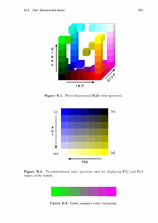
B.3. One-dimensional maps 211
Figure B.1. Three-dimensional RGB color spectrum.
Figure B.2. Two-dimensional color spectrum used for displaying PC1 and PC2values of the vowels.
Figure B.3. Green�magenta color continuum.


Appendix C
Vowel maps
This appendix includes maps that visualize the pronunciation of 19 di�erent vowelsof older and younger speakers at 98 sites in Sweden and the Swedish-language partsof Finland. The data is described in Chapter 4 in the thesis and the acoustic analysisof the vowel segments in Chapter 5.
As acoustic measures of vowel quality, two principal components (PCs) wereextracted from Bark-�ltered vowel spectra. The maps display the values of the twoPCs using a technique described in Appendix B (� B.2). The data from each site wasdivided into older and younger speakers (approximately six speakers per age groupper site), and the maps display the average PC scores in the two speaker groupsat each site. Values measured close to onset (at 25% of the vowel duration) andclose to o�set (75%) of the vowels are displayed separately. In each map, a StandardSwedish reference point is included in the upper left corner (rotated square). TheStandard Swedish vowels were recorded by six older and six younger speakers.
The maps are organized so that the Standard Swedish corresponding long andshort vowels (that is, long and short vowels written with the same orthographicsymbol) are placed adjacently when both vowels are present in the data set. Frontvowels are presented �rst, starting with the close front vowels and going on withmore open front vowels. After the front vowels the back vowels are presented in thereversed order, that is, starting with the most open back vowel and ending with theclosest one. A description and interpretation of all maps is given in � 6.1 in thethesis.
213

214 Appendix C. Vowel maps
onset old onset young
o�set old o�set young
Figure C.1. The vowel in the word dis. Standard Swedish /i:/. Described in � 6.1.1(p. 88).
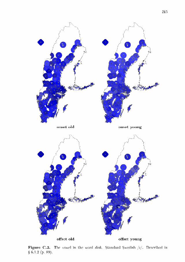
215
onset old onset young
o�set old o�set young
Figure C.2. The vowel in the word disk. Standard Swedish /I/. Described in� 6.1.2 (p. 89).

216 Appendix C. Vowel maps
onset old onset young
o�set old o�set young
Figure C.3. The vowel in the word typ. Standard Swedish /y:/. Described in� 6.1.3 (p. 90).
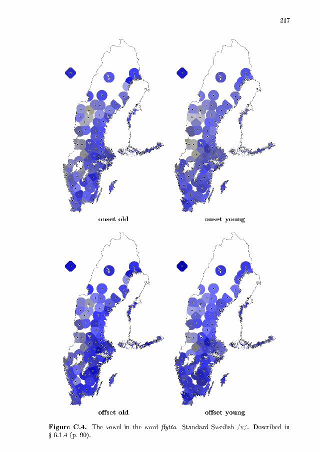
217
onset old onset young
o�set old o�set young
Figure C.4. The vowel in the word �ytta. Standard Swedish /Y/. Described in� 6.1.4 (p. 90).

218 Appendix C. Vowel maps
onset old onset young
o�set old o�set young
Figure C.5. The vowel in the word leta. Standard Swedish /e:/. Described in� 6.1.5 (p. 91).

219
onset old onset young
o�set old o�set young
Figure C.6. The vowel in the word lett. Standard Swedish /efl/. Described in � 6.1.6(p. 92).
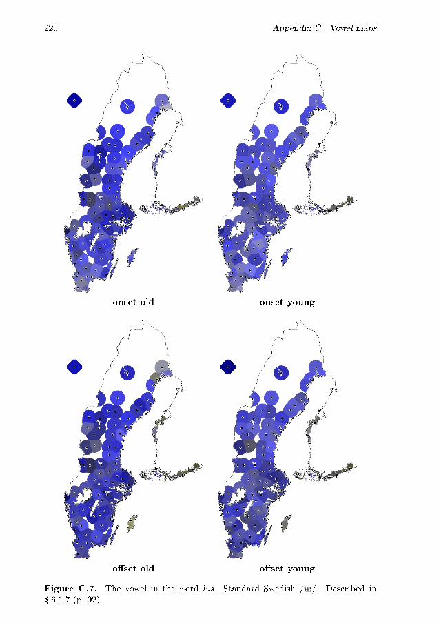
220 Appendix C. Vowel maps
onset old onset young
o�set old o�set young
Figure C.7. The vowel in the word lus. Standard Swedish /0:/. Described in� 6.1.7 (p. 92).

221
onset old onset young
o�set old o�set young
Figure C.8. The vowel in the word nät. Standard Swedish /E:/. Described in� 6.1.8 (p. 93).

222 Appendix C. Vowel maps
onset old onset young
o�set old o�set young
Figure C.9. The vowel in the word lär. The open allophone [æ:] of /E:/ in StandardSwedish. Described in � 6.1.9 (p. 94).

223
onset old onset young
o�set old o�set young
Figure C.10. The vowel in the word särk. The open allophone [æ] of /Efi/ inStandard Swedish. Described in � 6.1.10 (p. 96).

224 Appendix C. Vowel maps
onset old onset young
o�set old o�set young
Figure C.11. The vowel in the word söt. Standard Swedish /ø:/. Described in� 6.1.11 (p. 96).

225
onset old onset young
o�set old o�set young
Figure C.12. The vowel in the word lös. Standard Swedish /ø:/. Described in� 6.1.12 (p. 97).

226 Appendix C. Vowel maps
onset old onset young
o�set old o�set young
Figure C.13. The vowel in the word dör. The open allophone [œ:] of /ø:/ inStandard Swedish. Described in � 6.1.13 (p. 98).
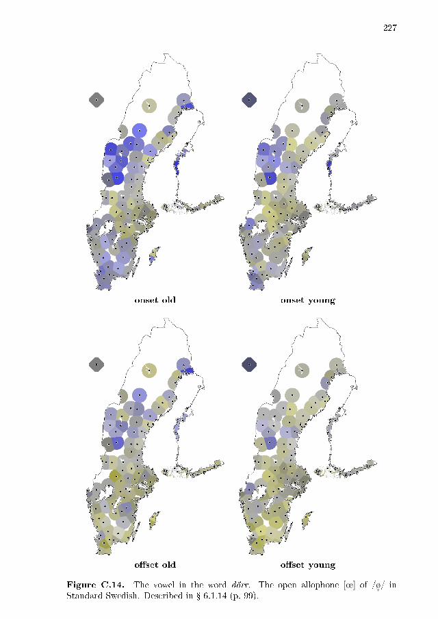
227
onset old onset young
o�set old o�set young
Figure C.14. The vowel in the word dörr. The open allophone [œ] of /øfl/ inStandard Swedish. Described in � 6.1.14 (p. 99).

228 Appendix C. Vowel maps
onset old onset young
o�set old o�set young
Figure C.15. The vowel in the word lat. Standard Swedish /A:/. Described in� 6.1.15 (p. 100).

229
onset old onset young
o�set old o�set young
Figure C.16. The vowel in the word lass. Standard Swedish /a/. Described in� 6.1.16 (p. 100).

230 Appendix C. Vowel maps
onset old onset young
o�set old o�set young
Figure C.17. The vowel in the words lås and låt. Standard Swedish /o:/. Describedin � 6.1.17 (p. 100).

231
onset old onset young
o�set old o�set young
Figure C.18. The vowel in the word lott. Standard Swedish /O/. Described in� 6.1.18 (p. 101).

232 Appendix C. Vowel maps
onset old onset young
o�set old o�set young
Figure C.19. The vowel in the word sot. Standard Swedish /u:/. Described in� 6.1.19 (p. 101).

Groningen Dissertations in
Linguistics (GRODIL)
1 Henriëtte de Swart (1991). Adverbs of Quanti�cation: A Generalized Quanti-�er Approach.
2 Eric Hoekstra (1991). Licensing Conditions on Phrase Structure.
3 Dicky Gilbers (1992). Phonological Networks. A Theory of Segment Repres-entation.
4 Helen de Hoop (1992). Case Con�guration and Noun Phrase Interpretation.
5 Gosse Bouma (1993). Nonmonotonicity and Categorial Uni�cation Grammar.
6 Peter Blok (1993). The Interpretation of Focus: an epistemic approach topragmatics.
7 Roelien Bastiaanse (1993). Studies in Aphasia.
8 Bert Bos (1993). Rapid User Interface Development with the Script LanguageGist.
9 Wim Kosmeijer (1993). Barriers and Licensing.
10 Jan-Wouter Zwart (1993). Dutch Syntax: A Minimalist Approach.
11 Mark Kas (1993). Essays on Boolean Functions and Negative Polarity.
12 Ton van der Wouden (1994). Negative Contexts.
13 Joop Houtman (1994). Coordination and Constituency: A Study in CategorialGrammar.
14 Petra Hendriks (1995). Comparatives and Categorial Grammar.
15 Maarten de Wind (1995). Inversion in French.
16 Jelly Julia de Jong (1996). The Case of Bound Pronouns in Peripheral Ro-mance.
233

234 GRODIL
17 Sjoukje van der Wal (1996). Negative Polarity Items and Negation: TandemAcquisition.
18 Anastasia Giannakidou (1997). The Landscape of Polarity Items.
19 Karen Lattewitz (1997). Adjacency in Dutch and German.
20 Edith Kaan (1997). Processing Subject-Object Ambiguities in Dutch.
21 Henny Klein (1997). Adverbs of Degree in Dutch.
22 Leonie Bosveld-de Smet (1998). On Mass and Plural Quanti�cation: The Caseof French `des'/`du'-NPs.
23 Rita Landeweerd (1998). Discourse Semantics of Perspective and TemporalStructure.
24 Mettina Veenstra (1998). Formalizing the Minimalist Program.
25 Roel Jonkers (1998). Comprehension and Production of Verbs in AphasicSpeakers.
26 Erik F. Tjong Kim Sang (1998). Machine Learning of Phonotactics.
27 Paulien Rijkhoek (1998). On Degree Phrases and Result Clauses.
28 Jan de Jong (1999). Speci�c Language Impairment in Dutch: In�ectionalMorphology and Argument Structure.
29 H. Wee (1999). De�nite Focus.
30 Eun-Hee Lee (2000). Dynamic and Stative Information in Temporal Reason-ing: Korean Tense and Aspect in Discourse.
31 Ivilin Stoianov (2001). Connectionist Lexical Processing.
32 Klarien van der Linde (2001). Sonority Substitutions.
33 Monique Lamers (2001). Sentence Processing: Using Syntactic, Semantic, andThematic Information.
34 Shalom Zuckerman (2001). The Acquisition of �Optional� Movement.
35 Rob Koeling (2001). Dialogue-Based Disambiguation: Using Dialogue Statusto Improve Speech Understanding.
36 Esther Ruigendijk(2002). Case Assignment in Agrammatism: a Cross-linguisticStudy.
37 Tony Mullen (2002). An Investigation into Compositional Features and FeatureMerging for Maximum Entropy-Based Parse Selection.
38 Nanette Bienfait (2002). Grammatica-onderwijs aan allochtone jongeren.
39 Dirk-Bart den Ouden (2002). Phonology in Aphasia: Syllables and Segmentsin Level-speci�c De�cits.

GRODIL 235
40 Rienk Withaar (2002). The Role of the Phonological Loop in Sentence Com-prehension.
41 Kim Sauter (2002). Transfer and Access to Universal Grammar in AdultSecond Language Acquisition.
42 Laura Sabourin (2003). Grammatical Gender and Second Language Processing:An ERP Study.
43 Hein van Schie (2003). Visual Semantics.
44 Lilia Schürcks-Grozeva (2003). Binding and Bulgarian.
45 Stasinos Konstantopoulos (2003). Using ILP to Learn Local Linguistic Struc-tures.
46 Wilbert Heeringa (2004). Measuring Dialect Pronunciation Di�erences usingLevenshtein Distance.
47 Wouter Jansen (2004). Laryngeal Contrast and Phonetic Voicing: A Laborat-ory Phonology Approach to English, Hungarian and Dutch.
48 Judith Rispens (2004). Syntactic and Phonological Processing in Develop-mental Dyslexia.
49 Danielle Bougaïré (2004). L'approche communicative des campagnes de sens-ibilisation en santé publique au Burkina Faso: les cas de la plani�cation fa-miliale, du sida et de l'excision.
50 Tanja Gaustad (2004). Linguistic Knowledge and Word Sense Disambiguation.
51 Susanne Schoof (2004). An HPSG Account of Non�nite Verbal Complementsin Latin.
52 M. Begoña Villada Moirón (2005). Data-driven identi�cation of �xed expres-sions and their modi�ability.
53 Robbert Prins (2005). Finite-State Pre-Processing for Natural Language Ana-lysis.
54 Leonoor van der Beek (2005). Topics in Corpus-Based Dutch Syntax.
55 Keiko Yoshioka (2005). Linguistic and gestural introduction and tracking ofreferents in L1 and L2 discourse.
56 Sible Andringa (2005). Form-focused instruction and the development of secondlanguage pro�ciency.
57 Joanneke Prenger (2005). Taal telt! Een onderzoek naar de rol van taalvaar-digheid en tekstbegrip in het realistisch wiskundeonderwijs.
58 Neslihan Kansu-Yetkiner (2006). Blood, Shame and Fear: Self-PresentationStrategies of Turkish Women's Talk about their Health and Sexuality.

236 GRODIL
59 Mónika Z. Zempléni (2006). Functional imaging of the hemispheric contribu-tion to language processing.
60 Maartje Schreuder (2006). Prosodic Processes in Language and Music.
61 Hidetoshi Shiraishi (2006). Topics in Nivkh Phonology.
62 Tamás Biró (2006). Finding the Right Words: Implementing Optimality The-ory with Simulated Annealing.
63 Dieuwke de Goede (2006). Verbs in Spoken Sentence Processing: Unravelingthe Activation Pattern of the Matrix Verb.
64 Eleonora Rossi (2007). Clitic production in Italian agrammatism.
65 Holger Hopp (2007). Ultimate Attainment at the Interfaces in Second Lan-guage Acquisition: Grammar and Processing.
66 Gerlof Bouma (2008). Starting a Sentence in Dutch: A corpus study of subject-and object-fronting.
67 Julia Klitsch (2008). Open your eyes and listen carefully. Auditory and au-diovisual speech perception and the McGurk e�ect in Dutch speakers with andwithout aphasia.
68 Janneke ter Beek (2008). Restructuring and In�nitival Complements in Dutch.
69 Jori Mur (2008). O�-line Answer Extraction for Question Answering.
70 Lonneke van der Plas (2008). Automatic Lexico-Semantic Acquisition forQuestion Answering.
71 Arjen Versloot (2008). Mechanisms of Language Change: Vowel reduction in15th century West Frisian.
72 Ismail Fahmi (2009). Automatic term and Relation Extraction for MedicalQuestion Answering System.
73 Tuba Yarbay Duman (2009). Turkish Agrammatic Aphasia: Word Order,Time Reference and Case.
74 Maria Tro�mova (2009). Case Assignment by Prepositions in Russian Aphasia.
75 Rasmus Steinkrauss (2009). Frequency and Function in WH Question Acquis-ition. A Usage-Based Case Study of German L1 Acquisition.
76 Marjolein Deunk (2009). Discourse Practices in Preschool. Young Children'sParticipation in Everyday Classroom Activities.
77 Sake Jager (2009). Towards ICT-Integrated Language Learning: Developingan Implementation Framework in terms of Pedagogy, Technology and Envir-onment.
78 Francisco Dellatorre Borges (2010). Parse Selection with Support Vector Ma-chines.

GRODIL 237
79 Geo�rey Andogah (2010). Geographically Constrained Information Retrieval.
80 Jacqueline van Kruiningen (2010). Onderwijsontwerp als conversatie. Prob-leemoplossing in interprofessioneel overleg.
81 Robert G. Shackleton (2010). Quantitative Assessment of English-AmericanSpeech Relationships.
82 Tim Van de Cruys (2010). Mining for Meaning. The Extraction of Lexico-semantic Knowledge from Text.
83 Therese Leinonen (2010). An Acoustic Analysis of Vowel Pronunciation inSwedish Dialects.
Grodil
Secretary of the Department of General LinguisticsPostbus 7169700 AS GroningenThe Netherlands