Ampacity Derating and Cable Functionality for - Raceway Fire ...

NUREG/CR-6681 SAND2000-1825

Ampacity Derating and Cable Functionality for Raceway Fire Barriers

Sandia National Laboratories

U.S. Nuclear Regulatory Commission Office of Nuclear Reactor Regulation Washington, DC 20555-0001

AVAILABILITY OF REFERENCE MATERIALS IN NRC PUBLICATIONS

NRC Reference Material

As of November 1999, you may electronically access NUREG-series publications and other NRC records at NRC's Public Electronic Reading Room at www.nrc.gov/NRC/ADAMS/index. html. Publicly released records include, to name a few, NUREG-series publications; Federal Register notices; applicant, licensee, and vendor documents and correspondence; NRC correspondence and internal memoranda; bulletins and information notices; inspection and investigative reports; licensee event reports; and Commission papers and their attachments.

NRC publications in the NUREG series, NRC regulations, and Title 10, Energy, in the Code of Federal Regulations may also be purchased from one of these two sources. 1. The Superintendent of Documents

U.S. Government Printing Office P. 0. Box 37082 Washington, DC 20402-9328 www.access.gpo.gov/su-docs 202-512-1800

2. The National Technical Information Service Springfield, VA 22161-0002 www.ntis.gov 1-800-533-6847 or, locally, 703-805-6000

A single copy of each NRC draft report for comment is available free, to the extent of supply, upon written request as follows: Address: Office of the Chief Information Officer,

Reproduction and Distribution Services Section

U.S. Nuclear Regulatory Commission Washington, DC 20555-0001

E-mail: DISTRIBUTION @nrc.gov Facsimile: 301-415-2289

Some publications in the NUREG series that are posted at NRC's Web site address www.nrc.gov/NRC/NUREGS/indexnum.html are updated periodically and may differ from the last printed version. Although references to material found on a Web site bear the date the material was accessed, the material available on the date cited may subsequently be removed from the site.

�1*

Non-NRC Reference Material

Documents available from public and special technical libraries include all open literature items, such as books, journal articles, and transactions, Federal Register notices, Federal and State legislation, and congressional reports. Such documents as theses, dissertations, foreign reports and translations, and non-NRC conference proceedings may be purchased from their sponsoring organization.

Copies of industry codes and standards used in a substantive manner in the NRC regulatory process are maintained at

The NRC Technical Library Two White Flint North 11545 Rockville Pike Rockville, MD 20852-2738

These standards are available in the library for reference use by the public. Codes and standards are usually copyrighted and may be purchased from the originating organization or, if they are American National Standards, from

American National Standards Institute 11 West 4 2 nd Street New York, NY 10036-8002 www.ansi.org 212-642-4900

The NUREG series comprises (1) technical and administrative reports and books prepared by the staff (NUREG-XXXX) or agency contractors (NUREG/CR-XXXX), (2) proceedings of conferences (NUREG/CP-XXXX), (3) reports resulting from international agreements (NUREG/IA-XXXX), (4) brochures (NUREG/BR-XXXX), and (5) compilations of legal decisions and orders of the Commission and Atomic and Safety Licensing Boards and of Directors' decisions under Section 2.206 of NRC's regulations (NUREG-0750).

DISCLAIMER: This report was prepared as an account of work sponsored by an agency of the U.S. Government. Neither the U.S. Government nor any agency thereof, nor any employee, makes any warranty, expressed or implied, or assumes any legal liability or responsibility for any third party's use, or the results of such use, of any information, apparatus, product, or process disclosed in this publication, or represents that its use by such third party would not infringe privately owned rights.

NUREG/CR-6681 SAND2000-1825

Ampacity Derating and Cable Functionality for Raceway Fire Barriers

Manuscript Completed: July 2000 Date Published: August 2000

Prepared by S. Nowlen

Sandia National Laboratories P.O. Box 5000 Albuquerque, NM 87185-0748

R. Jenkins, NRC Project Manager

Prepared for Division of Engineering Office of Nuclear Reactor Regulation U.S. Nuclear Regulatory Commission Washington, DC 20555-0001 NRC Job Code J2886

ABSTRACT

This report discusses two topical areas associated with localized fire barrier cladding systems for cables and cable raceways, namely, ampacity derating and cable functionality. Ampacity is defined as the electrical current carrying capacity of a particular cable in a given set of routing and environmental conditions. Ampacity derating refers to the process by which cable electrical current carrying limits are reduced in order to compensate for the thermal insulating effects of a raceway fire barrier cladding system. Cable functionality refers to the practice of assessing fire endurance ratings for a raceway fire barrier based on an assessment of the protected cables' ability to perform their intended design function before, during, and after the fire endurance exposure.

The discussions are based on experience and insights gained through reviews sponsored by the U. S. Nuclear Regulatory Commission (USNRC) of related licensee submittals. These reviews were conducted between 1994 and 1999 and involved a total of 23 USNRC licensees and numerous individual licensee submittals. In each topical area, the report provides general technical background, discusses currently applied methods of assessment, and identifies potential technical issues that may arise in the application of each assessment method. The report also provides guidance to assist the USNRC staff in reviewing and assessing licensee submittals in each area.

iii

TABLE OF CONTENTS

A B STRA CT ................................................................. iii

ACKNOW LEDGMENTS ...................................................... ix

ACRONYMS AND INITIALISMS ............................................... x

1 INTRODUCTION ........................................................... 1 1.1 O bjectives ....................................................... 1 1.2 Background ...................................................... 1 1.3 Report Structure and Organization .................................... 2

2 AMPACITY DERATING TECHNICAL BACKGROUND ........................... 4 2.1 Term inology ...................................................... 4 2.2 Basis and Nature of Potential Ampacity Derating Concerns ................. 6

2.2.1 Underlying Basis for Ampacity Concerns and Required Expertise ...... 6 2.2.2 Short-Term Operational Constraints ............................. 8 2.2.3 Long-Term Operational Constraints ............................. 9

2.3 Establishing the Acceptable Cable Operating Temperature Limits ........... 10 2.4 Establishing In-Plant Cable Loads .................................... 11 2.5 Factors of Importance to Ampacity Determination ....................... 12

2.5.1 Ambient Temperature ....................................... 12 2.5.2 Exposure to Sunlight ........................................ 13 2.5.3 Local Air Currents .......................................... 13 2.5.4 Cable Size and Conductor Count ............................... 13 2.5.5 Cable Routing or Raceway Type and Features .................... 14 2.5.6 Maintained Spacing Installation Practices ........................ 15 2.5.7 Raceway Grouping .......................................... 15 2.5.8 Raceway Cable Loading ...................................... 16 2.5.9 Fire Barrier Cladding .................................... 16 2.5.10 Passage Through a Penetration Seal ............................ 16 2.5.11 Cable Load Diversity ........................................ 16 2.5.12 Less than Nominal Voltage Conditions .......................... 17 2.5.13 Cable Voltage Rating ........................................ 17

3 AMPACITY AND AMPACITY DERATING METHODS .......................... 19 3.1 O verview ....................................................... 19 3.2 Methods for Determination of Baseline Ampacity ....................... 20

3.2.1 Open Air Applications ....................................... 20 3.2.2 Conduit Applications ........................................ 22

v

3.2.3 Cable Tray Applications ..................................... 23 3.2.4 Excluded Methods of Assessment .............................. 26

3.2.4.1 Excluded IPCEA P-46-426 Cable Tray Methods ............ 26 3.2.4.2 The Watts Per Foot Method ............................. 26

3.3 Methods for Determination of Ampacity Derating Factors ................. 27 3.3.1 Experimental Methods of Derating Assessment ................... 27 3.3.2 Analytical Methods of Derating Assessment ...................... 30 3.3.3 Thermal Similarity and Extrapolation of ADF Values .............. 32

3.4 Methods for Determining Clad Case Ampacity .......................... 34 3.4.1 Application of an ADF Factor ................................. 34 3.4.2 Direct Assessment of Clad Case Ampacity ....................... 34

3.5 Diversity M ethods ................................................ 36

4 AMPACITY DERATING REVIEW GUIDANCE ................................. 38 4.1 Consistency of Treatment for Baseline and Clad Cases ................... 38 4.2 Estimating Absolute Ampacity Versus Relative Derating Impact ............ 41 4.3 Thermal Model Validation .......................................... 42 4.4 Example Case Analyses ............................................ 44 4.5 Selection of Heat Transfer Correlations and Parameters ................... 44 4.6 Removal of Perceived Conservatism in Standard Tables .................. 46 4.7 Bounding Plant Operational Conditions ............................... 47 4.8 Reliance on Emergency Overload Ratings ........................... 48 4.9 Establishing Baseline Ampacity ..................................... 49 4.10 Extrapolation of Test Data and Verification of Thermal Similarity .......... 51 4.11 Consideration of Individual Cable Loads ............................... 52 4.12 Crediting Load Diversity ........................................... 52 4.13 Numerical or Implementation Errors .................................. 53

5 CABLE FUNCTIONALITY TECHNICAL BACKGROUND ......................... 55 5.1 Term inology ..................................................... 55 5.2 Basis and Nature of Potential Cable Functionality Concerns ............... 56 5.3 Cable Functionality Acceptance Criteria ............................... 57

6 CABLE FUNCTIONALITY ASSESSMENT METHODS ........................... 59 6.1 O verview ....................................................... 59 6.2 Direct Measurement of Cable Electrical Performance ..................... 59

6.2.1 O verview ................................................. 59 6.2.2 Direct Measurement Techniques ............................... 59

6.3 Indirect Analysis Cable Functionality ................................. 66 6.3.1 O verview ................................................. 66 6.3.2 Measurement and Analysis Techniques ........................... 69

vi

7 CABLE FUNCTIONALITY REVIEW GUIDANCE ............................... 73 7.1 Potential Areas of Technical Concern ................................. 73

7.1.1 Cable Sample Selection and Placement .......................... 73 7.1.2 Direct IR Monitoring Systems ................................. 73 7.1.3 Indirect Performance Analyses ................................ 74 7.1.4 Interpretation and Analysis of Test Data and Results ............... 75

8 REFERENCES AND GENERAL BIBLIOGRAPHY ............................... 78 8.1 Cited References .................. .............................. 78 8.2 A General Bibliography on Cable Ampacity and Fire Barrier Ampacity

D erating ........................................................ 80 8.2.1 Journal Articles and Conference Papers: ......................... 80 8.2.2 Standards ................................................. 82 8.2.3 Technical Review Letter Reports ................................ 83

Appendix A: The Thermal Conductivity of a Composite Cable Bundle ................ A- I

Appendix B: The Neher and McGrath Conduit Model ............................... B-1

Appendix C: The StolpefICEA Cable Tray Model .................................. C-1

Appendix D: The Harshe and Black Cable Tray Diversity Model ..................... D-1

Appendix E: The Leake Cable Tray Diversity Model ............................... E-1

Appendix F: The SNL Cable Tray Thermal Model ................................. F-I

Appendix G: Summary of USNRC Reviewed Ampacity Derating Experiments .......... G- 1

vii

List of Figures

6-1 A simple cable functionality monitoring circuit using a single voltage potential 60 applied to a single conductor cable. The circuit is capable of estimating the cable IR based on the measured voltage drop across the ballast resistor as discussed in the text.

6-2 Electrical schematic of a single voltage potential monitoring system applied to a 63 multiconductor cable. Note the switching controller is designed to select one conductor at a time to be energized while all others are grounded. A full measurement cycle sequentially energizes each conductor and measures leakage current. This approach can theoretically handle any number of individual conductors.

6-3 A single voltage source system applied to a multiconductor cable without a 64 switching system. Note that the individual conductors are ganged into two groups, one group energized and the second grounded. IR is determined for the energized conductors only and then only as a group.

6-4 An example of a cable monitoring circuit using two energizing voltage 65 potentials. Note the isolation of the raceway from ground by a ballast resistor and monitoring of the leakage current to ground.

6-5 Illustration of the IR versus temperature behavior of a typical cable insulation 67 material. This plot shows test data and a linear regression curve fit for a Brand Rex cross-linked polyethylene (XLPE) insulated 12 AWG 3-conductor cable. The data are from Table 4 of NUREG/CR-5655 (Ref. 25). Similar plots can be generated for any given cable type, size and voltage rating given test data that reports IR as a function of temperature.

viii

ACKNOWLEDGMENTS

The author wishes to thank Ronaldo Jenkins, Bernie Grenier, and Paul Gill, each of the Nuclear Regulatory Commission's Office of Nuclear Reactor Regulation, for their longstanding support of Sandia National Laboratories (SNL) in these efforts. Ronaldo Jenkins has made substantial technical

contributions to these efforts as well. In addition the author acknowledges the contributions of Tina Tanaka and Ron Dykhuizen, both of Sandia National Laboratories (SNL), to the technical accomplishments documented in this report.

ix

ACRONYMS AND INITIALISMS

ACF ampacity correction factor

ADF ampacity derating factor

ANSI American National Standards Institute

ASTM American Society of Testing and Materials

AWG American Wire Gage size rating protocol

EQ equipment qualification

GL Generic Letter

ICEA Insulated Cable Engineering Association

IEEE Institute of Electrical and Electronics Engineers

IPCEA Insulated Power Cable Engineering Association

IR insulation resistance

JCN Job Code Number

LOCA loss of coolant accident

MCM thousands of circular mils

NEC National Electric Code

NIST National Institute of Standards and Technology

NRR Office of Nuclear Reactor Regulation

PDR Public Document Room

RHR residual heat removal

SNL Sandia National Laboratories

TUE Texas Utilities Electric

TVA Tennessee Valley Authority

USNRC U.S. Nuclear Regulatory Commission

XLPE Cross-linked polyethylene

x

1 INTRODUCTION

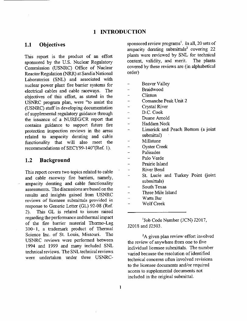
1.1 Objectives

This report is the product of an effort sponsored by the U.S. Nuclear Regulatory Commission (USNRC) Office of Nuclear Reactor Regulation (NRR) at Sandia National Laboratories (SNL) and associated with nuclear power plant fire barrier systems for electrical cables and cable raceways. The objectives of this effort, as stated in the USNRC program plan, were "to assist the (USNRC) staff in developing documentation of supplemental regulatory guidance through the issuance of a NUREG/CR report that contains guidance to support future fire protection inspection reviews in the areas related to ampacity derating and cable functionality that will also meet the recommendations of SECY99-140"(Ref. 1).

1.2 Background

This report covers two topics related to cable and cable raceway fire barriers, namely, ampacity derating and cable functionality assessments. The discussions are based on the results and insights gained from USNRC reviews of licensee submittals provided in response to Generic Letter (GL) 92-08 (Ref. 2). This GL is related to issues raised regarding the performance and thermal impact of the fire barrier material Thermo-Lag 300- 1, a trademark product of Thermal Science Inc. of St. Louis, Missouri. The USNRC reviews were performed between 1994 and 1999 and many included SNL technical reviews. The SNL technical reviews were undertaken under three USNRC-

sponsored review programs'. In all, 20 sets of ampacity derating submittals2 covering 22 plants were reviewed by SNL for technical content, validity, and merit. The plants covered by these reviews are (in alphabetical order)

- Beaver Valley - Braidwood - Clinton - Comanche Peak Unit 2 - Crystal River - D.C. Cook - Duane Arnold - Haddam Neck - Limerick and Peach Bottom (a joint

submittal) - Millstone - Oyster Creek - Palisades - Palo Verde - Prairie Island - River Bend - St. Lucie and Turkey Point (joint

submittals) - South Texas - Three Mile Island - Watts Bar - Wolf Creek

'Job Code Number (JCN) J2017, J2018 and J2503.

2A given plan review effort involved

the review of anywhere from one to five individual licensee submittals. The number varied because the resolution of identified technical concerns often involved revisions to the licensee documents and/or required access to supplemental documents not included in the original submittal.

I

Introduction

In addition, SNL reviewed cable functionality submittals for technical content, validity, and merit for two plants:

- Comanche Peak Unit 1 - Three Mile Island

Section 8.2.3 provides a complete bibliographic listing of SNL technical review letter reports generated as a result of these review efforts. These documents, while unpublished, are available through the USNRC Public Document Room (PDR). This report represents a consolidation of the findings and insights documented in these various reports.

1.3 Report Structure and Organization

This report covers two distinct but related topics: (1) assessing the impact of a raceway fire barrier system on the thermal environment experienced by the protected cables during normal operation (i.e., in the absence of an actual fire exposure) and the implication of these thermal changes on cable electrical current carrying capacity (ampacity) and (2) cable functionality assessments as a means of demonstrating adequate fire protection performance for a cable raceway fire barrier system. The report itself has been divided into six major sections, three devoted to ampacity derating (Sections 2-4) and three devoted to cable functionality (Sections 5-7). Each set of three sections covers general technical background, specific methods of assessment, and review guidance for each topical areas.

Each of the technical background discussion

sections (Sections 2 and 5) opens with a general and elementary background discussion. Their purpose is to (1) define the associated technical jargon that will be used in the more detailed discussions that follow and (2) familiarize the reader with the basic technical concepts and issues being addressed.

Sections 3 and 6 cover the various methods of assessment that are commonly applied in each topical area. For each method, the discussion will include identification of potential technical concerns that might arise as well as common approaches taken to resolve each concern.

Finally, a separate section is provided for each topical area containing specific review guidance (Sections 4 and 7). This guidance is intended to support the USNRC staff in the review and assessment of licensee submittals for each of these areas. The guidance is presented in a broadly based format. That is, the guidance is not necessarily tied to specific methods of assessment, but rather includes discussions of broad areas of potential technical concern, many of which will be applicable to several, if not all, assessment methods. (For example, the adequacy of a method's validation is a potential concern for almost any method that might be applied. Hence, guidance with regard to validation is discussed once in each of the two review guidance subsections.)

In general, this report focuses on both general and specific assessment methods available to licensees, rather than on the approaches taken by individual licensees. Many licensees have applied similar or identical methods of assessment while others have employed unique methods. This report will consolidate

2

Section I

Introduction

the associated review findings into a single discussion of each approach encountered in the reviews. Individual licensee submittals are not generally referenced or cited unless there is a specific objective to be served in doing so. As noted above, Section 8.2.3 provides a listing of past technical review findings documents.

Supplemental information is provided in the form of seven appendices. These appendices provide technical discussions of specific topics of interest. Appendix A presents the results of USNRC-sponsored tests that

measured the equivalent thermal conductivity of a composite cable bundle. Appendices B-G provide detailed discussions of various methods of ampacity and ampacity derating analysis. Included with the discussion of specific analysis methods are numerical/computer implementations of each method either as a FORTRAN computer program or implementations using a commercially available symbolic mathematics software program. For each such case a full listing of the numerical implementation is provided.

3

Section I

2 AMPACITY DERATING TECHNICAL BACKGROUND

2.1 Terminology

Before discussing specific issues associated with ampacity derating, it is useful to establish a common terminology. The area of ampacity uses jargon that is not typically applied to other aspects of nuclear power plant systems.

Throughout this report, references are made to cable raceways. A raceway is simply the physical support structure provided to aid in the routing of cables through a plant. The most common raceways encountered in fire barrier applications are cable trays (of various types) and conduits. Other raceways include wire-ways, bus ducts, cable gutters and underground or embedded duct banks. Fire barriers may also be encountered in an air drop application, but an air drop is not strictly classified as a raceway. Rather, an air drop is a cable run with no supporting raceway. A common example would be the cables that drop from an overhead cable tray into the top of an electrical panel.

This report also makes repeated references to localized raceway fire barrier systems. Indeed, the fire performance and thermal impact of raceway fire barriers is the entire focus of this report. A localized raceway fire barrier system refers to any one of many products used to form a protective envelope around an individual cable or cable raceway.'

3Note that localized fire barriers may also be used to protect other types of electrical equipment such as individual components or junction boxes. This report, however, focuses specifically on cable and cable raceway fire barrier systems.

The barrier system is designed to protect the cables inside the envelope from the damaging effects of a fire occurring outside the envelope. The fire barrier envelope will typically include one or more layers ofthermal insulation, may involve active or intumescent materials, and may also include surface radiant energy barriers (reflective foils for example). The overall objective of the envelope is to delay or prevent heat generated by the external fire from causing failure of the protected cables. Such barrier systems were used by many licensees in their efforts to achieve separation of fire safe shutdown systems and equipment as mandated in 10 CFR 50 Appendix R (or other applicable fire protection regulations).

The term ampacity, as used in this report, is defined as the maximum current carrying capacity of a given cable conductor applied in a given installation configuration. A cable's ampacity is dependent on its routing and installation configuration. That is, the same cable will have a variety of individual ampacity values depending on how and where it is installed. For example, a cable may have ampacity values associated with open air, conduit, and cable tray applications, each of which will be unique. Furthermore, other factors beside the raceway type impact ampacity including environmental ambient temperature, loading conditions (number of cables in the raceway), and grouping of raceways. Hence, ampacity is not a single valued property of a given cable, but rather, is a context-driven value that must be determined (or conservatively bounded) for each application of interest.

Throughout this report, reference is made to

4

Section 2

the baseline and clad cases. These terms, and in particular the terms clad case or clad ampacity, are unique to the issue of localized fire barriers for the protection of cables. In this context, the baseline case refers to the cable or raceway as it would exist in the absence of any fire barrier protection. This will be the case for which the standard ampacity tables are consulted to establish the baseline ampacity (typically denoted Ib'elrie in this report). The clad case is the raceway configuration where the exact same raceway is considered with the exact same cable loading, but with the fire barrier wrap (or cladding) in place. Analysis of the clad case yields the clad ampacity (typically denoted Iclad in this report).

The term ampacity derating refers to the practice of reducing ampacity to reflect some particular aspect or feature of a cable's installation configuration. To explain further, various features associated with how a cable is routed may adversely impact its current carrying capacity or ampacity. However, not all such features are accounted for in the standard tables of cable ampacity. It is common practice to begin with an ampacity value from a case covered by the industry ampacity standards and to then reduce cable ampacity to account for a range of relatively simple configuration features through a "derating" process. Ampacity derating maybe used to account for a range of factors including changes in ambient temperature, grouping of cable raceways (particularly conduits), and grouping of cables within a raceway (e.g., for multiple cables in a common conduit or tray). In this particular report, ampacity derating due to the installation of a protective fire barrier wrap

Ampacity Derating Technical Background

that envelopes a cable raceway is the topic of particular interest. For a fire barrier ampacity derating assessment, this always involves consideration of a baseline and a clad case, always taken in matched pairs. That is, for each clad case there is a corresponding baseline case that may well be unique. In some few cases, a conservative or bounding baseline case may be selected to represent a number of clad cases, but in general, the baseline and clad cases represent unique configuration pairs.

The ampacity derating factor, or ADF, is an expression of the relative reduction in cable ampacity (i.e., the derating impact) associated with a particular installation feature. The feature of interest to this report is installation of raceway fire barrier systems, a feature not covered by any of the existing ampacity standards. ADF is normally expressed as a percentage and is often used to extend the ampacity derating results for one test or analysis case to other thermally similar cases. That is, the testing of one raceway may be used as the basis for derating many other raceways that are thermally similar, a concept that will be explained in detail in the body of this report. To illustrate, consider a cable in a cable tray application where the baseline ampacity has been established as 100 A. If that raceway were then clad with a fire barrier system that was found through testing or analysis to have a 30% ADF, then this same cable would have a derated clad ampacity of 70 A reflecting a 30% reduction in ampacity. For fire barriers, ADF is based on comparison of the baseline and clad case ampacity values determined either by testing or analysis as follows:

5


ADF=100xa 1 Iclad M

i b aseline ( ) (

The ampacity correction factor, or ACF, is an alternate expression of the relative ampacity derating impact associated with a particular installation feature. The ACF and ADF are closely related, but are not directly interchangeable. ACF is normally expressed as a decimal fraction rather than as a percentage. Furthermore, the ACF reflects the fraction of the normal or baseline cable ampacity that is allowable given a particular installation feature or configuration. Hence, if the ACF of a fire barrier is equal to 0.7, then a cable with a baseline ampacity of 100 A would have a derated or clad ampacity when installed in the fire barrier system of 70 A. Again we see a 30% reduction in ampacity. Thus, the relationship between ADF and ACF is expressed as:

ADF Iclad AC100 = clad 10O0 'baseline (2)

Conductor insulation and cable jacketing are also important and distinct terms. The insulation is the material that immediately surrounds a cable's metal conductor and provides electrical isolation of the conductor from both other conductors and ground. Most modem insulation materials used in nuclear power plant cable systems are based on silicone, rubber, or other polymeric or thermosetting materials. In contrast, a cable jacket is an outer sheath that is applied to a cable to provide physical protection. A cable may be comprised of one or more conductors; hence, a cable jacket may envelope one or more conductors as well. The jacket is not intended by the manufacturer to provide any

Section 2

electrical function. It is purely a mechanical binding and physical protection sheath. Hence, the jacket plays no significant role in an assessment of cable functionality or electrical integrity. The jacket will, however, play a role in an ampacity assessment because it represents an additional thermal layer that must be accounted for in the ampacity thermal analysis.

Load diversity is a term that refers to the fact that in most real applications individual cables within a raceway will be loaded to various levels in comparison to the ampacity limit of each cable. That is, some cables may be normally de-energized (e.g., spares or abandoned cables), some may carry only a fraction of their rated ampacity, and others may be loaded to their full ampacity limits. In most of the traditional methods of analysis, load diversity is not credited and all cables are assumed to be operating at their full rated ampacity (see, for example, ICEA P-54-440) (Ref. 3). However, recent methods have been developed that explicitly credit load diversity (Refs, 4, 5, 6). Care must be taken to ensure that an adequate basis is established if load diversity is being credited in an ampacity or ampacity derating analysis.

2.2 Basis and Nature of Potential Ampacity Derating Concerns

2.2.1 Underlying Basis for Ampacity Concerns and Required Expertise

In assessing a licensee's treatment of cable ampacity, the reviewer should recognize one very important fact; namely, the concerns associated with cable ampacity all boil down to a question of the operating temperature of

6

Section 2

the cables. That is, the objective of any ampacity assessment is ultimately to ensure that cables are operating withing acceptable temperature limits. Cable conductors (copper and aluminum) are not perfect electrical conductors; rather, they retain some ohmic resistance to electric current flow. Resistance is inversely proportional to a conductor's cross-sectional area, and directly proportional to conductor length and temperature. Hence, the flow of current in a cable creates resistance heating, and the greater the current, the greater the resistance heating load. This resistance heating load must be continuously rejected to the ambient environment to achieve steady state operating conditions. As a result, the steady state operating temperature of the cable will be greater than that of the surrounding environment. As the rate of current flow in the cable increases, so does the operating temperature of the cable. To keep the cable from overheating, the current load must be limited.

Given this view, one should also recognize that the assessment of cable ampacity is far more appropriately characterized as a thermal or heat transfer problem than as an electrical problem. The level of electrical expertise required to perform or review an ampacity or ampacity derating assessment is quite modest for most common cases. One must have an understanding of Ohm's law, the theory of resistance heating, and the electrical properties of aluminum and copper conductors including the effects of temperature on conductor resistance. It is also desirable that the reviewer have an understanding of basic cable construction practices, cable insulation materials, and basic cable routing design features and practices. In some few cases, questions of inductive currents may arise


(electrical current flow in an electrically conductive media that is "induced" by proximity to a current carrying conductor). The resolution of these issues does require a knowledgeable electrical expert. This is, however, rarely a factor in a day-to-day assessment of cable ampacity and ampacity derating.

In contrast, the ampacity analyst or reviewer should possess a firm grounding in heat transfer behavior and analysis. Most ampacity assessments involve the application of thermal models in some form. These models may be those upon which the standard ampacity tables are based or may be customized thermal models. In either case, the models can be quite complex. Even in a relatively straight forward derating assessment, an analyst may extrapolate available test data to the fire barrier systems of interest. A thorough understanding of heat transfer behavior is required so that the reviewer can judge the appropriateness of the extrapolation basis.

All aspects of heat transfer - conduction, convection, and radiation - play a role in an ampacity assessment. Based on the USNRC and SNL experience in the review of licensee responses associated with Generic Letter (GL) 92-08 (Ref. 2), if issues arise in the review of an ampacity or ampacity derating assessment, it is far more likely that they will be associated with thermal modeling than with the electrical aspects of the analysis. Many of the USNRC reviews identified thermal modeling concerns whereas very few identified electrical concerns. The thermal modeling concerns ranged from simple mistakes made in the implementation of a model to questions regarding the selection and basis of the thermal modeling correlations used. Points of

7


potential concern based on past reviews are discussed in detail in Chapter 4.

The need to maintain cables within acceptable operating temperature limits derives from two potential concerns. The first is related to short-term behavior and the second is related to long-term behavior. Ultimately, as discussed below, it is the long-term behavior that dominates the ampacity assessment. These short- and long-term concerns are discussed in the following two sub-sections.

2.2.2 Short-Term Operational Constraints

The first, and perhaps most obvious, temperature limit of potential concern is the ultimate temperature limit beyond which the conductor insulation cannot maintain adequate electrical isolation of the cable conductor(s). For most of the commonly used modern insulation materials, insulation resistance falls exponentially as temperature increases (there are exceptions associated, for example, with fire-rated cables). At some point, the drop in insulation resistance will lead to immediate electrical failure (short circuits).

Even at temperatures below the point where loss of insulation resistance becomes an immediate concern, softening of the insulation materials may occur, depending on the material. Softening may lead to physical contact between conductors or between a conductor and ground. This softening is commonly characterized by a "glass transition temperature," and this temperature may be substantially lower than the temperature at which insulation resistance would fall below an "acceptable" level. Hence, both behaviors are important to cable performance.

Section 2

In the short-term view, ampacity must be limited in order to ensure that these ultimate performance limits of the conductor insulation are not exceeded. This leads directly to the concept of a cable's "emergency overload" ampacity rating. However, these short-term concerns have little or no relevance to the determination of day-to-day cable ampacity. The emergency overload rating is just what the name implies - an ampacity rating that be relied upon should only under very unusual or emergency conditions during which a cable might be subjected to a short-term current load in excess of its steady state or nominal ampacity limit. As such it is inappropriate to establish a cable's normal, anticipated day-today operating capacity on the emergency overload rating even for short duration loads (e.g., a motors in-rush startup load). In fact, industry standards establish stringent limits on the number of occurrences during which a cable might operate at these elevated ampacity levels over the course of its entire lifetime. (Ref. 7). This issue is discussed further in Section 4.8 in the context of resolution of nominally overloaded cables.

The failure to appropriately limit cable ampacity can lead to short-term problems. These problems will typically be manifested relatively early in a plant's operating lifetime. Indeed, severe cable overloads would generally be reflected as "infant mortality" failures. The fires that occurred at San Onofre during 1968 are examples of such incidents (Ref. 8). In this case, a severe cable overload condition led to fires on two occasions early in the plant's operating lifetime. Reviewers of an ampacity study must be cognizant of these short-term concerns but will more likely find themselves focusing on the corresponding long-term concerns.

8

Section 2

2.2.3 Long-Term Operational Constraints

The primary constraint in ampacity limits derives from long-term concerns. A cable is expected to perform its design function even following many years of day-to-day operation. This constraint leads to the second temperature limit of interest, namely, the temperature at which continuous operation will not compromise a cable's ability to perform its design function for the anticipated lifetime of that cable.

As discussed above, cables are subject to electrical self-heating by virtue of the fact that current is flowing through an imperfect conductor (copper or aluminum). The higher the current load, the higher the heat load and the higher the operating temperature of the cable. The maximum current load (ampacity) of a cable is limited such that the cable's operating temperature will remain within its design limit. In the context of ampacity, longterm concerns lead to more limiting ampacity values than do short-term immediate fault concerns.

These long-term performance concerns are also inseparably tied to the insulation aging behavior. As modem insulation materials age, their physical and electrical properties change. Cable aging is primarily an oxidation process that takes place over a period of many years (Ref. 9). The most obvious effect of aging is a stiffening or embrittlement of the jacket and insulation materials. This embrittlement increases the potential that cracks might form in the insulation, and cracking of the insulation can lead to electrical failure.

It is also well known that as the temperature


increases, the rate of insulation material aging also increases. (Exposure to ionizing radiation also accelerates the aging process, but this in not a topic relevant to this report.) A very rough "rule of thumb" states that for every increase in cable temperature of 10'C (for example from 50'C to 60'C), the life expectancy of a cable is cut in half.4 Indeed, the entire field of Equipment Qualification (EQ) testing is based largely on this concept; namely, that increases in temperature result in predictable acceleration of the aging process (Ref. 10). Hence, one can simulate the end of life conditions (e.g., the conditions after 40 or 60 years of continuous operation at a given temperature) through accelerated aging of the materials for a much shorter period of time in a higher temperature environment (as short as 30 days or less is not uncommon).

Exactly the same concepts can be applied directly to the ampacity problem. As noted above, higher current loads imply higher

operating temperatures for a given cable in a given installation configuration. Hence, operation at current loads that exceed the cable's ampacity implies operation at temperatures that exceed the temperature design limit of the cable. In the short-term view, this may lead to immediate cable

failures. However, in the long-term view, operation at excessive temperatures leads to accelerated aging of the cable, leading to premature degradation of the cable such that

4This concept is only approximately true (i.e., a "rule of thumb"). The actual temperature- aging rate correlation for a given material is governed by a property called the "activation energy" and each material has a unique activation energy.

9


long-term survival/performance might be threatened. The temperatures associated with the onset of long-term aging concerns are far lower than those associated with the onset of short-term failure. That is, a cable that is expected to operate for 40 or 60 years must be operated at temperatures well below the limits at which short-term failure might become a problem. Hence, the long-term constraints dominate the ampacity assessment process.

2.3 Establishing the Acceptable Cable Operating Temperature Limits

The actual acceptable operating temperature, or design temperature limit, of a given cable may depend on both the cable itself and on its design function. The cable itself is important because the operating temperature will be a function ofthe cable's material properties, and in particular, the insulation material properties. Design function may also play a role for certain cables required for plant safety following a design basis loss of coolant accident (LOCA). These cables may be subject to EQ harsh environment survival constraints, and these constraints maybe more restrictive than the constraints applied in areas not subject to those same harsh environments.

The most commonly cited operating temperature limit is that set by the cable's manufacturer. These values are based primarily on the cable insulation material properties. For general applications, most modem cables are rated by the manufacturer for continuous operation at temperatures up to 90 0 C although exceptions certainly exist. Manufacturer ratings are based on the operating temperature of the conductor itself

Section 2

(as compared to the cable outer surface temperature, for example). This represents the worst-case temperature to which the insulation should be subjected, that is, the temperature at the point of contact between the conductor and the insulation.

Cables that are subject to USNRC EQ requirements may be subject to more stringent operating temperature conditions. This is because the cables are required to demonstrate a higher level of performance at their end of life (operation under LOCA conditions) than general application cables installed elsewhere in the plant. There were no cases encountered in the USNRC reviews of licensee Generic Letter 92-08 (Ref. 2) responses where the EQ concerns overlapped the fire barrier ampacity derating concerns. All of the review efforts described here were based on consideration of the more generous manufacturer cable operating temperature limits rather than EQbased limits.

The two temperature ratings, EQ versus ampacity, are not directly comparable and should not generally be viewed as directly interchangeable. EQ assessments commonly consider the full life-time exposure history of a cable whereas an ampacity derating assessment uses a more conservative approach to the estimation of cable operating temperatures. Hence, it is generally inappropriate to mandate that an ampacity assessment be based on the commonly applied conservative methods of ampacity assessment while at the same time using the equipment qualification temperature limits as the basis for analysis. If an ampacity derating and EQ application overlap, then some special consideration of cable load factors and duty cycles may well be warranted. Methods have

10

Section 2

been published by which the actual life expectancy of a cable can be estimated based on the actual operating conditions of that cable (Ref. 11).

2.4 Establishing In-Plant Cable Loads

A second fundamental aspect of an ampacity analysis is characterization of cable electrical current loads as they exist in the plant. In this assessment, it is important that the analysis consider all modes of plant operation. For example, it is common practice to provide no specific analysis for cables that are not continuously energized. However, care must be taken in defining what constitutes a continuous power load. In general, any load that persists for about an hour or more during any mode of plant operation constitutes a continuous power load that should be assessed in the ampacity analysis. It is assumed that one hour provides sufficient time for the cable to approach its continuous operating temperature. For example, a cable that may not be used during power operations may be used during shutdown operations (e.g., residual heat removal [R-IR] pump power cables) and vice-versa (e.g., main feedwater pump power cables). It is important for the ampacity analysis to consider various operational modes in assessing cable loads. Specific areas to be considered in cable loads include the following:

A common practice is to assess all cable loads based on the sum total of the current draw of all devices powered by that cable without consideration of which devices might be operating at any given time. This


approach inherently captures, in a

conservative manner, all possible modes of plant operation.

It is common to neglect cables that carry only intermittent power loads, such as control and power cables to motor-operated valves. In this context, any load that might persist for about an hour or more should be included in the assessment.

It is common to neglect the load current on instrumentation cables.

In assessing loads for energized cables, the presence of nonenergized cables must also be considered as a factor in the analysis. For example, nonenergized cables still contribute to raceway fill and do need to be addressed accordingly.

Identifying cable loads is of particular interest in cases where cable load diversity is being credited. In this case, the diversity analysis should consider that certain cables may carry loads during certain modes of operation and not during other modes. It may be appropriate for licensees to provide complementary analyses for

various plant operating modes, or to provide a single analysis that conservatively bounds all modes of operation.

In the characterization of cable loads, it may be necessary to consider emergency modes of plant operation. For example, operation of the diesel generators during a loss of offsite

11


power event introduces unique power loads on the associated power feed cables that are not present during normal operations. These loads also need to be considered in the ampacity assessment.

2.5 Factors of Importance to Ampacity Determination

In addition to the cable's operating temperature limit (discussed above), there are several factors that impact the ampacity of a cable. These factors may be associated with the ambient environment, the cable raceway type, the raceway routing configuration, cable loading configuration, and special features such as fire barrier wraps. This section provides an overview of those factors that are most commonly encountered in an ampacity or ampacity derating study. The list is not exhaustive for all applications but covers all factors that might arise in a fire barrier ampacity derating assessment.

2.5.1 Ambient Temperature

The local ambient temperature is a very important factor in the assessment of cable ampacity. In this case, the local ambient is most commonly the air within a room through which the cable passes. In certain applications, the temperature of the ground or an external ambient may apply.

As discussed above, a cable's ampacity is ultimately set so as to ensure that the cable itself does not exceed its design temperature. This operating limit is based on the actual temperature of the cable's metal conductors

Section 2

while in operation. However, the ability of the cable (or cable raceway) to reject heat is dependent on the temperature difference between the cable and the local ambient, a basic concept of heat transfer. As the ambient temperature increases, the raceway's heat rejection capacity decreases. As a result, cable ampacity (and therefore the heat load) must be decreased.

It is common practice to base plant-wide ampacity assessments on a single ambient temperature that conservatively bounds (i.e., on the high side) all plant areas, plant operating conditions, and seasonal variations. In some cases, separate ambient temperature constraints might be established for individual plant areas. This technique is common for plant areas with substantially higher temperature environments (e.g., 50'C for specific areas versus a plant wide 40'C ambient).

The most commonly applied ambient temperature limit used in the U.S. nuclear industry is 40'C (104'F). This value bounds most common applications. Use of a lower value should be accompanied by a specific justification. Use of a higher value may also be appropriate for some plant areas (e.g., areas with poor ventilation or with high concentrations of steam piping), or for plants in particularly hot regions of the country. The selected value should bound the actual plant conditions. Bounding is discussed further in Section 4.7.

12

Section 2

2.5.2 Exposure to Sunlight

Direct exposure of a cable or raceway to sunlight can sharply impact cable ampacity. Direct solar exposure increases the heat load on a cable or raceway and may sharply limit rejection of heat through thermal radiation. Direct exposure to sunlight is rarely a concern in nuclear power plant assessments. With some few case specific exceptions, the only cables likely to be subject to direct sunlight would be those cables associated with off-site power and potentially those associated with the plant diesel generators. For plants that have open air configurations,5 or where cables have been routed along the outside of a building,' some cables may be subject to direct solar heating and this should be considered in the analysis. However, for most plants, most cables are routed' in interior spaces shielded from direct solar heating. Sunlight exposure is routinely considered in the routing of large outdoor power cables, and the newer ampacity standards for these applications, i.e., the Institute of Electrical and Electronics Engineers (IEEE) Standard 835-

5For example, in the southeastern United States, some plants have structures composed of various open deck configurations rather than fully enclosed buildings.

6Routing along a building exterior, for example, might be encountered in cases where cable routing was changed in response to the 10 CFR 50 Appendix R separation criteria, and where the most expedient reroute involved placement of cables in trays or conduits along exterior walls.


1994 [Ref. 16] includes sunlight corrections while the more commonly applied Insulated Cable Engineering Association (ICEA) and National Electric Code (NEC) tables do not.

2.5.3 Local Air Currents

The movement of air in the vicinity of a cable or raceway (or the lack thereof) can also impact cable ampacity. Enhanced air flow increases the rates of convective heat transfer. In general, some additional ampacity load may be allowable if the cable in question is subject to a continuous and active means of air flow, for example, through an actively ventilated bus duct. The newer ampacity tables of IEEE 835-1994 reflect this potential impact directly, although the older and more commonly applied ICEA and NEC standards do not. For nuclear power plant applications, it is commonly assumed that cables are in a still-air environment and no credit is taken for local air flow, this being the most conservative approach. Assumption of an ambient air flow condition should be accompanied by an explicit justification.

2.5.4 Cable Size and Conductor Count

The physical size of a cable and the conductor count within a cable (or raceway) also impact ampacity. The most direct impact is associated with the wire gage of the individual conductors. Larger diameter conductors can quite obviously carry higher current loads in a given application (due to the reduction in residual electrical resistance). However, other aspects of cable size may also impact ampacity.

One factor that contributes to size is the conductor count. A single cable may contain

13


several conductors, and as the count increases, the cable physical size also increases. The most commonly encountered cables are of a 1,2-, or 3-conductor configuration, particularly considering power cable applications, but virtually any conductor count is possible. Communication cables for example may easily have as many as 50 or more conductor pairs. As the number of conductors increases, the ampacity limits generally decrease. Standard ampacity tables explicitly provide for 1- and 3-conductor cable configurations, again because these are the most common configurations for power cable applications. The NEC Handbook provides a correction factor for higher conductor counts (the same conductor count correction factors are applied for both conduits as a whole and individual cables) (Ref. 12).

One must also exercise some caution because increasing cable diameter for a given wire gage does not always lead to decreased ampacity. For open air and conduit applications (ICEA P-46-426), ampacity decreases with increasing cable diameter. In these applications, the increased thermal insulation associated with increasing insulation and jacket thickness dominates the assessment. However, for cable tray applications (IPCEA P-54-440), just the opposite is true. For example, given two single conductor cables with the same wire gage in a cable tray, the larger diameter cable will have a higher ampacity limit. This is because the Stolpe method for cable trays (Ref. 13) assumes that the overriding factor in cable trays is, in effect, power density, which translates as the heat generated per foot of tray per unit of tray cross-section. That is, the cable tray analysis method determines an overall cable tray heat load and then

Section 2

distributes that load evenly over the crosssectional area of the tray. Hence, a larger cable gets a greater heat load allocation and will be found to have a higher ampacity than a smaller cable with the same wire gage. This result is somewhat counter-intuitive, and in extreme cases might lead to anomalous results (e.g., in the analysis of a very small conductor with an excessively thick insulation/jacket layer). However, such extreme cases are unlikely and this approach is accepted practice; based on available test results the approach appears to work well for cable trays where the packing density is generally high.

2.5.5 Cable Routing or Raceway Type and Features

The characteristics of the raceways through which a cable passes also impact ampacity. Standard ampacity tables are provided for many common routing configurations including separate tables for open air applications (i.e., no raceway), conduits, cable trays, direct burial, and duct banks. In general, it is desirable to apply the standard tables directly when possible. However, even for a given raceway, specific features of the raceway may impact ampacity. For example, cable trays may be covered by a solid steel plate (either as a fire barrier or as physical protection). The use of a steel cover will reduce cable ampacity and must be accounted for in the assessment. These factors are commonly addressed through a derating analysis.

14


2.5.6 Maintained Spacing Installation Practices

For cable trays there is one particular method of cable routing known as "maintained spacing" can substantially impact ampacity. Under this approach, cables are individually secured to the cable raceway in such a manner that no two cables ever come into contact with each other. Note that simply strapping down the cables in an orderly fashion does not constitute a maintained spacing installation. Rather, a proper installation (as defined by ICEA P-46-426, Section IL.D.1) will have no direct contact between cables and will have an air gap between any adjacent cable pair equal to or greater than one-fourth of the diameter of the larger cable. Hence, the overall tray load will be quite sparse, commonly less than one full layer of cables, although maintained vertical spacing is also allowed. Under these conditions, heat transfer from the cables is less restricted, and more generous ampacity loads are allowed than would apply to a more densely loaded tray or to a "random fill" tray where the cable spacing is not maintained. The ICEA tables for open air ampacity limits (Ref. 14) also cover maintained spacing applications for cable trays, as discussed in Section 3.2.3 below. In practice, this method will be encountered most commonly in installations of larger power cables and then only on a plant-specific basis.

2.5.7 Raceway Grouping

The grouping of cable raceways can also impact ampacity. Explicit guidance is provided for the grouping of conduits and for the grouping of bus-ducts (Ref. 14). No explicit guidance is available, however, for the grouping of cable trays, and most ampacity

assessments will neglect this potential effect. The exception would be raceway fire barrier ampacity analyses involving stacked cable trays in a common enclosure. In such cases, the baseline case may have explicitly modeled the unclad stacked configuration, although a single tray may also be used as the baseline case as well. For this configuration, the clad analysis would be expected to treat the mutual heating effects of the multiple stacked cable tray because the fire barrier system has created an intimate link between the behavior of the clad trays.

It is common practice in U.S. nuclear power plants to place the cables with the highest heat loads in the topmost trays7. Hence, it is common to see "power over control over instrumentation" configurations of cable trays. This configuration tends to minimize the mutual heating effect of one tray upon another. Hence, the grouping of cable trays should not be a significant concern for most U.S. nuclear power plant applications. However, it must also be recognized that since there is no explicit practice for grouping-based ampacity derating for cable trays, allowances for such grouping effects must be bounded by the margin that is inherent in the base ampacity standards themselves. This is one reason why the technical reviews described in this report have been reluctant to grant relaxation of the perceived conservatism in the standard ampacity tables. That is, the tables must bound some factors that are not explicitly considered in an ampacity analysis, and grouping of cable trays is one such factor.

7Based on discussions with USNRC NRR staff.

15

Section 2


2.5.8 Raceway Cable Loading

The number of cables (or cable conductors) housed within a common raceway generally has a substantial impact on cable ampacity. For conduits, ampacity estimates should include a correction factor based on the number of energized conductors present (Ref. 12). These factors represent substantial ampacity reductions for conductor counts greater than three.

For cable trays, the critical factor is the depth of fill of cable in the tray. This factor can be used as a surrogate for the cable or conductor count. The greater the depth of fill, the lower will be the cable ampacity. This principle accounts for the insulating effect experienced by cables located in the center of the cable mass. The existing standards applied to random fill cable tray explicitly consider tray fill in determining ampacity (Ref. 3).

2.5.9 Fire Barrier Cladding

As discussed extensively elsewhere in this report, fire barrier cladding is another factor commonly addressed through the ampacity derating process. The actual ampacity derating impact of a fire barrier can be substantial (e.g., some cases approaching a 60% ADF have been observed). The actual impact for a given barrier system depends on the properties of the fire barrier materials as well as installation practices. Material properties of particular importance include thermal conductivity and surface emissivity. (Note that ampacity derating involves steadystate heat transfer calculations only so transient heat transfer properties such as density and thermal diffusivity are not important.) Installation features of importance

Section 2

include the material thickness, the presence of air gaps between material layers, and application of surface treatments, especially those intended to act as radiant energy shields (such as a foil outer surface coating). The actual configuration of the barrier may also be important, for example, installation on a single raceway versus a common enclosure for two or more raceways. This point is covered in more detail in other sections of the report.

2.5.10 Passage Through a Penetration Seal

Cables that pass through a fire barrier penetration seal can also be subject to ampacity derating. The most common penetration seal material is silicone foam. These seals may be several inches thick. Silicone is a poor conductor of heat, which is one of the properties that makes it a good choice as a fire barrier material. However, this poor heat conduction can also create local hot-spots that may become the limiting factor in a cable's ampacity assessment. This configuration is not a major point of discussion in this report, but there are articles available in the public literature on this topic (Ref. 15).

2.5.11 Cable Load Diversity

As noted above, load diversity reflects the fact that in practice not all cables in a raceway will be operated at their maximum ampacity limit. The reduction in overall raceway heat load due to load diversity may allow for the energized conductors to carry a larger ampacity load than would be allowed under the traditional methods of analysis. Most of the traditional methods of analysis do not credit diversity and conservatively assume that all cables are fully loaded when determining

16

Section 2

ampacity limits. Methods have been developed that take explicit credit for load diversity in estimating ampacity limits including two that have been reviewed by the USNRC (see Section 3.5).

The earliest of the diversity methods is arguably the ICEA P-46-426 correction factors for cables in cable trays without maintained spacing (Ref. 14). These factors were based on the total conductor count in the tray and did "include the effects of load diversity." Early versions of the NEC Handbook later adopted the same adjustment factors for conduit applications, again based on conductor count, and again citing that diversity was included in the development of the factors (Ref. 12). In both cases it was explicitly stated that a 50% load diversity was assumed. That is, the values assumed that no more than half of the conductors would be carrying current at any given time. More recently published versions of the NEC now cite more conservative correction factors for cases where diversity cannot be assumed or assured. (The original diversity-based values are still cited as appendix material.)

Stolpe also considered the problem of load diversity in his pioneering work on cable trays (Ref. 13). However, it was his recommendation that diversity not be credited in cable tray ampacity. Stolpe's concerns centered on the potential that allowing for diversity credits in cable trays might lead to adverse groupings among the more heavily loaded cables and a localized overheating problem (see further discussion of Stolpe's observations in Section 3.5). This problem would be very difficult to control, and might lead to subsequent problems. The USNRC has recently reviewed two methods of


diversity analysis for cable trays (Ref. 4, 6). The licensee submittals associated with these reviews were accepted by the USNRC by demonstrating that the ampacity derating concerns of GL 92-08 had been resolved and final approval was based on application of modified versions of these methods (see Section 3.5 and Appendices D and E).

2.5.12 Less than Nominal Voltage Conditions

The consideration of less than nominal voltage conditions can also impact an ampacity assessment. Basically, under less than nominal voltage conditions a motor, for example, may draw more than the nominal rated current flow in order to draw the same power load. Normally, it is not expected that an ampacity assessment will explicitly consider less than nominal voltage conditions. However, if it is determined that a particular application is subject to frequent operation under less than nominal voltage conditions, then some attention to the impact on ampacity may be warranted.

2.5.13 Cable Voltage Rating

The voltage rating of a cable is based primarily on the insulation material and thickness. Cables of higher voltage rating generally have a larger outside diameter than equivalent gage cables with a lower voltage rating. In open air and conduit applications, the extra thickness of insulation on the higher voltage rated cables leads to a reduced ampacity in comparison to lower voltage cables (see ICEA P-46-426). The standard ampacity tables for these applications explicitly address voltage rating.

17


In the case of cable trays, the opposite effect is observed (see IPCEA P-54-440). As discussed in Chapter 3 below, the standard ampacity tables for random fill trays are based on a model that assumes uniform heat generation per foot of tray per unit of crosssectional area through the cable mass. The estimated maximum total heat load is then

Section 2

allocated to individual cables based on the fraction of the cross-sectional area that is represented by each cable. Hence, a larger diameter cable will be allowed a greater ampacity than an equivalent cable of smaller diameter. This result is somewhat counterintuitive, but is accepted practice.

18

3 AMPACITY AND AMPACITY DERATING METHODS

3.1 Overview

This section discusses known baseline ampacity assessment and ampacity derating methods. Recall that ampacity derating can be used to account for a variety of installationspecific factors that impact ampacity. In this particular report, we are concerned with ampacity derating as applied to a localized raceway or cable fire barrier system. A typical fire barrier ampacity derating assessment is comprised of four steps. The first involves the determination of the baseline ampacity. In this case, this implies the ampacity in the absence of a raceway fire barrier system. The second step involves the determination of the ADF factor associated with the fire barrier system. The third step is the determination of the clad case ampacity limit. The fourth step is the assessment of in-plant service loads and the resolution of any identified current overload conditions. The subsections that follow focus on the first three steps in this process. The resolution of identified overload conditions is taken up in Section.

Section 3.2 covers the available baseline ampacity methods. It is important that the reviewer understand baseline ampacity methods because mistakes made in the assessment of baseline ampacity transfer directly to the analysis of the clad case under most methods of analysis. It should also be noted that baseline ampacity assessment methods generally derive from industry standards. These standards have not been explicitly reviewed nor endorsed by the USNRC. The methods of analysis applied vary widely depending, in particular, on the type of raceway or routing the applicable to a given cable. Hence, Section 3.2 is divided

into three sub-sections to address each of the primary cable routing and raceway configurations that are encountered in nuclear power raceway fire barrier applications; namely, cable air drops (no raceway), conduits, and cable trays.8

Section 3.3 discusses methods for the determination of an ADF for a raceway fire barrier system. In general, there are two approaches to this determination: an experimentally based assessment and an analytical estimation. Both of these approaches are discussed in Section 3.3.

Section 3.4 is relatively brief and discusses the methods for determining the clad case ampacity limits, which commonly involves application of an ADF value to the baseline ampacity. However, there are also some methods wherein the clad case ampacity limits are assessed directly (i.e., without explicit consideration of a corresponding baseline case). Both approaches are covered in Section 3.4.

The final section in this chapter, Section 3.5, takes up the specific topic of methods that

8Note that certain other routing configurations that may be encountered in a nuclear power plant are neglected here because they would not be subject to protection by a fire barrier system. This group includes cables in duct banks and direct burial of cables. Both routing configurations involve variations on the open air ampacity methods. Other configurations such as cable gutters or wireways are simply extrapolations of the other methods that are explicitly covered.

19

Ampacity and Ampacity Derating Methods

explicitly credit load .diversity. This area of ampacity assessment is continuing to be developed by industry. Hence, this is an area that may require specific attention in future review efforts. In many ways, the diversity methods have yet to be fully proven for general applications, and the two methods that have been reviewed by the USNRC were modified by the submitting licensees to ensure that the results retain an adequate level of conservatism.

3.2 Methods for Determination of

Baseline Ampacity

3.2.1 Open Air Applications

Open air applications are those applications where a cable is routed through open air in the absence of a cable raceway support structure. The most common example of such an application is overhead power lines. In nuclear power plants, the more common example would be cable air drops in which a cable drops out of an overhead raceway and into an electrical panel. In some very limited cases, one might also argue that the open air ampacity values can be applied to a cable in a open cable tray; however, this would require an exceedingly light cable load in the tray, such as, a single cable routed by itself in a tray.

The open air ampacity is generally the most generous possible ampacity limit to which a cable will be subject. That is, the ampacity in open air will exceed the ampacity in most any other installation configuration including, in particular, conduits and cable trays. In most cases, the open air ampacity will not be the limiting configuration of a cable in a nuclear

Section 3

power plant. Most cables will at some point be routed through at least one cable tray or conduit, and the ampacity for the cable overall will be limited by the raceway conditions rather than by the open air conditions. Open air ampacity limits are most commonly drawn from one of four sources.

For the U.S. nuclear industry, the most commonly cited source is the Insulated Power Cable Engineering Association9 standard IPCEA P-46-426 ampacity tables Ref. 14). These tables were first published in 1943 and were updated in 1954. They continue to see wide use today. The standard covers a range of cable wire gage sizes ranging from 8 AWG through 2000 MCM.'0 It also covers single conductor, triplex," and three conductor power cables. Values are also given for a range of cable voltage ratings and for a range of ambient and cable operating temperature conditions.

9Note that the Insulated Power Cable Engineering Association (IPCEA) is now know as the Insulated Cable Engineering Association (ICEA). Standards are cited per their actual identification as IPCEA or ICEA documents.

'OAWG refers to the American Wire Gage size rating protocol, and MCM stands for thousands of circular mils, a sizing standard commonly used for larger power cables.

"A triplex cable is a set of three single conductor cables twisted together. they are common in three-phase power applications and in overhead power distribution applications.

20

Section 3

The second most commonly cited source is the NEC Handbook (Ref. 12).. This source covers many of the same applications as the ICEA standard cited above, and for these common applications the ampacity values are quite similar although not identical (the differences are not considered significant). The advantage of the NEC Handbook is that it covers smaller wire gage sizes (down to 14 AWG in some cases) and two conductor applications as well. An additional advantage is that ampacity correction factors are cited to adjust the ampacity limits for conductor counts of greater than three in a common cable (the same factors also apply to conduits, as discussed in Section 3.2.2). These correction factors are commonly applied in the same mantner to ampacity values taken from other sources.

The third source most commonly cited is manufacturer data. In reality, for most cables, the manufacturers simply cite the ampacity values from either the ICEA or NEC Handbook as applied-to their particular cables. In some cases, manufacturers will have performed ampacity tests for unique cable constructions that are not explicitly covered by the standard tables. These values are acceptable for use in an ampacity assessment provided that a licensee can document the source of the values applied (i.e., that they can cite and have available the specific manufacturer documents that provide the ampacity values).

The final source of open air ampacity limits is the more recently published IEEE standard 835-1994 (Ref 16). Development of this standard began in the late 1970s as an update to the IPCEA P-46-426 tables. The standard was ultimately delayed due to the effort


required to develop the revised tables and a lack of financial support for this activity. Ultimately the standard was published in 1994. The same cables and applications are covered by the IEEE standard and in the same format as those covered by the P-46-426 tables. The changes in ampacity limits are generally very modest. In the specific case of conduits, some ampacity limits have been reduced based on more advanced modeling approaches. However, the reductions are generally modest. Some changes can also be attributed to the consideration of direct solar heating and ambient air flow conditions that was added to the IEEE tables. When applied in nuclear plant applications, it is common to apply the "no sun" "0 m/s air flow" conditions. Because the IEEE standard is relatively new, it was not used by most plants in their original design and is therefore not the "code of record" in this regard. Hence, the IEEE standard was not widely cited in the licensee submittals reviewed by SNL and the USNRC.

In general, the available ampacity tables have been developed based on analytical assessments of cable ampacity. These analytical methods were developed based on experimental results, but most of the cases covered by the tables have not been explicitly tested. One advantage of the ICEA standard is that the tables include the specific modeling parameters assumed in the analysis of each case cited in the tables. This listing includes parameters such as the external thermal resistance, cable conductor diameter, cable outer diameter, etc. These values are found in a separate table following each of the specific case applications cited in the standard. This method does allow one to directly verify the ampacity modeling results. It can also provide

21


a basis for comparing licensee cited modeling parameters to those that govern the standard tables.

Regardless of the source, application of the open air ampacity table is generally a relatively straight-forward process. The user simply selects the appropriate cable size and configuration, goes to the appropriate table, applies the prevailing ambient and cable temperature conditions, and reads the desired ampacity value from the table. For the IEEE standard, the "no sun" / "0 m/s" column should be applicable to most cases.

Difficulties can arise in cases involving smaller conductors or conductor counts not covered by the tables. In these case,s one generally has three choices: (1) select a bounding case and accept the implied conservatism, (2) apply the NEC conductor count correction factors, or (3) estimate the ampacity limit using the same modeling tools as were applied in the development of the standard tables. The third option is relatively easy to accomplish given the ICEA and IEEE standards, which clearly document the analysis process used and include specific case examples.

3.2.2 Conduit Applications

In the case of cables routed in conduits, the sources for baseline ampacity data are essentially identical to those cited in Section 3.2.1 for open air applications. That is, IPCEA P-46-426, IEEE 835, the NEC Handbook, and manufacturer data are all applied in determining conduit ampacity values. The process of application is also essentially identical to that described above for open air applications.

Section 3

The one added factor that must be considered in conduit applications is the potential presence of multiple cables in a common conduit. For this case, the NEC conductor count correction factors for cables and conduits can be applied to the baseline ampacity for each energized conductor. It is important to note that the conductor count is based on the total number of energized conductors within the conduit, not on the conductor count for a given cable, nor the cable count within the conduit.

There are actually two sets of the conductor count correction factors. The original set was published in the body of the NEC through 1987 and inherently credited a 50% load diversity factor. That is, these values assumed that no more than half of the conductors would actually be carrying a load current. This assumption led to an increased ampacity allowance for those conductors that were energized and carrying current. Many early ampacity studies failed to note this constraint and applied the correction factors without verifying that the assumed diversity did, in fact, exist. Since 1988, a new set of correction factors that assumes no load diversity has been published in the body of the NEC Handbook. The diversity-based values have been moved to Appendix B of the Handbook. The newer values are more restrictive (i.e., lead to lower ampacity limits).

In the application of the conductor count correction factors, it is appropriate either to apply the newer and more restrictive values that assume no load diversity, or to require that verification of a 50% load diversity be provided in order to justify application of the older diversity-based values. In some of the past reviews, licensees argued that accepted

22

Section 3

practice at the time was based on the more generous values and that to require demonstration of diversity or application of the nondiversity values represented a "backfit" requirement. This argument was, however, rejected on the basis that the original published values very clearly stated that a 50% load diversity was assumed. The failure to verify the applicability of these values given this cited assumption was deemed to be an oversight and error in the original analyses. Hence, requests to either justify the application of the diversity-based correction factors or to apply factors that do not credit diversity were found to be technically appropriate.

In the specific case of conduits, the methods of analysis are rather more complicated than those that are applied to open air installations. Indeed, conduit thermal models represent the most complicated of the three commonly encountered applications for the nuclear power applications (open air, conduits, and cable trays). In particular, there is the additional complication of thermal interactions between the cables and the interior of the conduit. Because the geometry is inherently two-dimensional, the considerations become more complex. In particular, the calculations must bound the worst-case configurations of a cable embedded in a cable bundle or a cable on top of the cable bundle, in either case, cables that do not directly contact the surface of the conduit. This adds an additional level of complexity to the thermal problem in that heat transfer internal to the conduit involves conduction, internal confined space convection, and thermal radiation all occurring in a complex two-dimensional geometry with internal heat generation that


may be nonuniform.

The published ampacity tables for conduits all derive from the methods of analysis developed by Neher and McGrath in the late 1950s (Ref. 17). The Neher/McGrath method is fairly complex, was validated by extensive experimental data at the time of development, and involves the application of a number of empirical correlations. These correlations are often worked through a series of transformations and approximate forms. Hence, one must exercise caution in the application of this approach to ensure that consistent parameter values and definitions are applied. The work of Neher and McGrath is widely considered one of the pioneering studies in the field, and the validity of the approach has not been seriously challenged despite significant changes in cable manufacturing and materials that have been realized since the work was first published. The Neher/McGrath method remains an accepted method of practice today. Appendix B provides a more detailed discussion of the Neher/McGrath method and includes a MATHCAD implementation of the model constructed by SNL for use in simple applications.

3.2.3 Cable Tray Applications

Baseline ampacity values for cables in cable trays are obtained from one of two sources. The choice depends on the installation configuration. The two configurations are maintained spacing (see Section 2.5.6) and random fill cable trays. A random fill tray is any tray that does not meet the requirements of a maintained spacing installation. That is, random fill does not necessarily imply a disorderly installation arrangement. It simply

23


implies that no measures are taken to prevent contact between cables in the tray.

Maintained spacing installations are covered by IPCEA P-46-426. In particular, Section II.D.1 and Table VII of the subject standard address maintained spacing installations. Basically, the open air ampacity limits are adjusted to account for the proximity to other cables using correction factors. These correction factors are, in effect, ampacity correction factors or ACFs. The choice of the factor to be applied is based on the number of cable rows and columns located in the tray (i.e., the cable tray cross-section is viewed as a two-dimensional matrix of individually separated cables in rows and columns).

Random fill cable trays are explicitly covered by a second standard, ICEA P-54-440. This standard derives directly from the pioneering work of Stolpe (Ref. 13) and utilizes the same basic thermal model as that developed by Stolpe. The model assumes that the cables in the tray form a composite cable mass of uniform depth (the cable tray depth of fill) and spreading across the full width of the tray. It is also assumed that every cable in the cable tray is operated at its ampacity limit; that is, no credit is taken for load diversity. The approach further assumes that the critical parameter characterizing the limiting cable ampacity is the rate of heat generation per foot of tray length per unit of cross-sectional area represented by the cable mass. This value is assumed to be uniform across all cables in the tray regardless of their size or wire gage. That is, the total heat load is allocated to individual cables in direct proportion to their contribution to the total cross-section of the cable mass. Appendix C provides a more detailed description of the Stolpe/ICEA model

Section 3

and includes a MATHCAD implementation of the model assembled by SNL for use in simple applications.

In practice, the ICEA P-54-440 tables were generated by exercising Stolpe's onedimensional thermal model of the cable mass. This model estimates the peak, or hot-spot, temperature within the cable mass as a function of the total heat generation rate, depth of fill, and ambient conditions. The heating rate is adjusted until the hot-spot temperature matches the design temperature of the cables in the tray. The total heating load is then allocated to individual cables based on their contribution to the total cable mass cross-sectional area. Individual cable ampacities are then calculated based on the conductor resistance and the total number of conductors in the cable so as to match that cable's heat load allocations (i.e., ohmic heating matches the heat load allocation for each cable).

The model has been exercised for a wide range of cases involving single-conductor, triplex, and three-conductor cables of various voltage ratings, various depths of fill, and wire gage. Simple corrections can be made to the tabulated values to account for different cable diameter or ambient conditions. For any case not explicitly covered by the tables (for example, a seven-conductor cable), a simple exercising of the thermal model as documented in Appendix B of the standard (or that described in Appendix C of this report) readily yields the desired ampacity. In theory, the Stolpe/IPCEA method can assess the ampacity load for any cable in any cable tray. The ability to directly extrapolate the method to any installation and any cable is one of its great advantages. The thermal model is also

24

Section 3

quite simple to understand and implement. However, the method does have some potential pitfalls, which include the following:

The Stolpe/ICEA method can yield unrealistic results in some situations. In particular, when there are large diameter cables in an otherwise lightly loaded cable tray, the direct modeling estimates of ampacity can easily exceed the open air ampacity limits for the same cable. This is a known flaw in the approach and a potential problem in any application where the diameter of any individual cable exceeds the depth of fill for the tray overall. In order to address this flaw, the standard specifically limits cable ampacity in random fill trays to 80% of the corresponding ampacity in open air. This particular constraint is easily overlooked in applications of the method, particularly when an analysis implements and exercises its own version of the StolpeiICEA model. Reviewers should carefully assess such analyses to ensure that the 80% limit has been appropriately applied.

A second aspect of the Stolpe/ICEA model that is often confused is the definition of cross-sectional area and the corresponding definition of depth of fill applied. This is the one area where the original Stolpe work and the ICEA standard differ. Stolpe's original work estimated the crosssectional area and depth of fill by summing the actual cross-section of each cable, assuming each cable had a circular cross-section. In contrast, the ICEA standard estimates cross-section


and depth of fill by summing the individual cable cross-sections, but the cross-section of each cable is assumed to be a square region with sides equal to the diameter of the cable. So long as one is consistent, there is minimal difference in the final results (no case encountered by SNL ever resulted in an ampacity difference of more than 1 A for any given situation). However, errors can arise if the two definitions are mixed in a single calculation. For example, if the total heat load is calculated using Stolpe's round cable approach, and the heat load is then allocated using the ICEA square cable approach, nonconservative ampacity results will be obtained. In this case, consistency is the key to correct answers.

A third aspect of the thermal model that has also been the subject of some recent investigation is the assumed value of the thermal conductivity of the composite cable mass. In reality, the cable mass is made up of copper and/or aluminum conductors, insulation materials, jacket materials, various filler materials used in the cable manufacturing process, and air gaps. However, in the thermal model, the cables are assumed to be a single homogenous thermal mass characterized by a single thermal conductivity value. Stolpe assumed a composite thermal conductivity value of 0.26 W/mr!K although the basis for this value cannot now be reconstructed. As a part of the USNRC sponsored efforts at SNL, a pair of simple tests was conducted to

25


assess the thermal conductivity for two cable bundles. Documentation of these tests is included as Appendix A to this report. The results showed thermal conductivity values that were substantially lower than the values assumed by Stolpe (i.e., 0.15-0.18 W/m/IK). A higher thermal conductivity, as assumed by Stolpe, would generally lead to more generous ampacity limits. However, it was also concluded that Stolpe's apparently optimistic thermal conductivity simply compensated to some extent for other sources of conservatism in the model based on the good agreement of his model and experiments. In general, continued application of the Stolpe values in the existing practice is the preferred approach provided that the other aspects of the model are preserved intact. This method maintains consistency with the existing standards and tables. However, in cases where other aspects of the Stolpe model are modified such that conservatism is relaxed, or where a unique model is developed abandoning the Stolpe approach, use of values based on experiments such as those performed by SNL would be appropriate.

3.2.4 Excluded Methods of Assessment

3.2.4.1 Excluded IPCEA P-46-426 Cable Tray Methods

Sections II.D.2 and II.D.3 of IPCEA P-46-426 discuss ampacity limits for ladder and solid bottom cable trays where the spacing is not maintained. Correction factors are presented

Section 3

in Table VIII that correct the open air ampacity limits based on the total number of conductors present in the tray." This approach has been explicitly superceded by the ICEA P-54-440 standard (see the "History" section of P-54-440). Hence, these factors should not be applied in any nuclear power plant applications as the basis for assessing ampacity for cables in random fill cable trays. Instead the ICEA P-54-440 approach should be applied. Note that this does not impact the maintained spacing approach set forth in IPCEA P-46-426 Section II.D.1.

3.2.4.2 The Watts Per Foot Method

One particular class of analysis methods that was put forth by certain licensees is known collectively as the Watts Per Foot approach. Under this approach, the underlying assumption is that the critical factor in estimating the allowable ampacity load for a given raceway is the total heat load on the raceway. Under this approach, an analysis will first sum the heat loads for each individual conductor in the raceway to obtain a total heat load for the raceway as a whole. This calculation is typically done using actual in-plant current loading conditions for each cable. This total heat load is then compared to an acceptance criteria, often derived from one of the standard ampacity tables. Provided that the total heat load is below the acceptable

"2Note that the cited correction factors are identical to those cited in older versions of the NEC Handbook for multiconductor cables and conduits. In this case, they again state that the effects of load diversity are included.

26

Section 3

raceway heat load, it is concluded that the individual cable current loads are within acceptable limits.

The critical flaw in this approach is the lack of a systematic partitioning of the total raceway heat load to the individual cables contained in the raceway. That is, the method fails to consider the actual acceptability of individual conductor or cable load currents.

As an example of this flaw's impact, consider a large and heavily loaded cable tray. The overall heat load on this tray would be quite substantial assuming that all of the cables are operating at their appropriate ampacity limits per the ICEA standard. If, in a specific case, there were actually only one cable in the tray that was energized and carrying current, then the Watts Per Foot approach would allow for the allocation of the entire tray thermal load to this one cable. The overall thermal loading for the raceway assumes uniform distribution of the heat load over the full cross-section of the cables. To concentrate this same heat load into a single cable would lead to inappropriate levels of localized heating in the vicinity of that cable.

An ampacity assessment must systematically assess the appropriateness of individual cable loads. A number of variations of the Watts Per Foot method were encountered in the USNRC reviews and all were rejected as inappropriate. Reviewers should carefully review any ampacity analysis that purports to assess cable ampacity limits based on total raceway thermal loads without explicitly comparing individual cable loads to their corresponding individual ampacity limits.


3.3 Methods for Determination of

Ampacity Derating Factors

Recall that an ADF is an expression of the percentage drop in ampacity that is realized due to a change in some aspect of the installation configuration for a given cable. While many installation factors can be addressed through application of an ADF, the specific topic of interest to this report is raceway fire barrier systems. These systems do impact the thermal conditions of the protected cables, and therefore do impact the ampacity of the protected cables. The ADF is a general measure of this impact that can then be applied to a range of thermally similar applications.

Two general approaches can be taken to establish ADF values: an experimental approach and an analytical approach. Subsections 3.3.1 and 3.3.2 discuss these two approaches. The concept of thermal similarity and ADF extrapolation is taken up in Section 3.3.3.

3.3.1 Experimental Methods of Derating Assessment

An experimental assessment of the ampacity derating factor or ADF is based on the comparison of two test results. One result represents the baseline case, and one the clad case. In the past, there was no standard that specified an ampacity derating protocol. Tests were generally performed by the manufacturer of a particular barrier product, by a scientific researcher interested in the topic, or by the end users of a particular barrier product. Hence, the early ampacity derating tests were each unique. This situation led to considerable

27


uncertainty regarding the validity and accuracy of the cited results. However, more recent tests have followed standard protocols and have avoided these problems. Appendix G of this report provides a summary of the currently available tests that have directly explored ampacity derating effects for fire barriers and have been reviewed by the USNRC. Note that all of the reviewed tests relate to resolution of the fire barrier performance issues raised with regard to the fire barrier material Thermo-Lag"3 per Generic Letter 92-08 (Ref. 2).

In recent years, IEEE has published a new standard protocol for ampacity derating tests for fire barrier installations, IEEE 848 (Ref. 18). The USNRC did have input into the development of this standard. Nearly any test sample can be tested based on the IEEE testing protocol, but the standard covers, in particular, an individual cable in open air, one or more cables in conduit, and cable trays.

The test protocol requires that each test (the baseline and clad cases) be performed in a controlled environment so that the ambient temperature is maintained at a constant value of 40'C (104'F). For each test, the current load on the cables is slowly increased until the hot-spot temperature in the sample cables reaches a steady state condition equal to the cable's continuous operating temperature rating, generally 90'C (194 0 F). Thermocouples are installed in the cable samples at specified intervals for this purpose. These thermocouples must be installed below

'3Thermo-Lag is a trademark product of Thermal Science Inc. of St. Louis, Missouri.

Section 3

the cable insulation and in contact with the cable conductors (i.e., the desired temperature is the conductor temperature, not the cable surface temperature).

Because in practice, the desired ambient and cable hot-spot temperature conditions cannot be achieved exactly, a correction is made to adjust each of the two final measured current values to the desired standard conditions. The current load that produces the standard condition is taken as the ampacity for that case (baseline or clad). The test is repeated for the cable/raceway in both the baseline and clad conditions. The order of testing is not important (i.e., the clad test may be run first). Once the two tests have been run, the two ampacity values are compared, as shown in Section 2.1. The result is an estimate of the fire barrier ADF (or ACF) for the given installation configuration.

In theory and in practice, an ampacity derating test is a relatively straightforward but timeconsuming task. Substantial time is typically devoted to installation of the fire barrier system in particular. The actual test specimens (trays or conduits in particular) maybe pre-constructed and used repeatedly by the testing laboratory. In particular, cable tray specimens that comply with the standard are commonly constructed once, and then tested repeatedly for different fire barrier systems as needed.

Potential pitfalls to the ampacity derating testing approach should be considered in the review of a testing report. These include the following items:

The baseline and clad tests should be performed using exactly the same

28

Section 3

physical test specimen and cables. It was found in early applications of the draft standard that use of different test specimens could produce anomalous results. This was observed in particular for conduits due to variations in the conduit surface emissivity. However, it is now considered accepted practice to base all derating tests on the actual testing of the same test specimen in both the clad and baseline condition.

It is inappropriate to compare a clad case ampacity limit determined by testing to a baseline ampacity value taken from a standard ampacity table. This was one approach that had been allowed in drafts of the IEEE standard. However, the final standard no longer allows this practice. Reviewers should be cognizant of this change. Under existing practice, the ADF should be based on two actual experimental results for the same test specimen.

Seemingly minor variations in the ambient conditions can impact the ampacity results. In tests sponsored by the USNRC (Ref. 19), it was observed that simply turning the lights on and off in the environmental test cell produced a visible impact on the measured temperature response of the test article. Hence, it is important that both the baseline and clad tests be performed under environmental conditions as nearly identical as is practical to achieve. One specific potential problem to watch for is a testing laboratory that relies upon a


past test of the baseline test sample for comparison to future clad case tests. That is, the laboratory may have past results for the same baseline test article, and may then test only the clad case comparing the new and old results to estimate ADF. This method may be acceptable, but would require that the lab demonstrate that no changes have been made in the environmental conditions that might impact test results. For example, if the new test were run in a different environmental chamber, or if substantive changes where made in the environmental chamber between the two tests, then the results may be invalidated. This situation may require that the test lab re-run the baseline case under the modified environmental conditions to verify the validity of the test results.

The instruments used to measure temperature response and current loading should be properly calibrated at the time of the tests. National Institute of Standards and Technology (NIST) protocols are the currently accepted basis for calibration at most testing laboratories.

Achieving a proper steady state condition is a long and tedious process for a typical ampacity test, but is critical to obtaining valid results. The test standard provides a specific approach for demonstrating steady state has been achieved.

Some anomalies may be observed in any test set. This does not necessarily

29


invalidate a test set. Any anomalies observed during testing should be noted in the test documentation and assessed for their potential impact on the test results.

It is quite typical that a test report will provide results for a number of test specimens, rather than for a single test specimen. Cross-comparison of the test results can often reveal undetected test anomalies. As noted above, recent testing performed concurrent with development of the IEEE testing standard revealed the potential pitfalls of using different test specimens for the baseline and clad cases. This was discovered by personnel doing the tests based on the cross comparison of test results which revealed inconsistencies in the behavior of nominally similar test articles. In the USNRC reviews, one case emerged in which a cross-comparison of test results revealed an apparent previously undetected test anomaly. When questioned on this point, the testing laboratory and licensee conceded that an undetected anomaly had occurred, and this ultimately led to the invalidation of one particular test pair from the overall test set (the remaining tests were accepted).

3.3.2 Analytical Methods of Derating Assessment

In a fundamental sense, an analytical assessment of fire barrier ADF values follows the same pattern as the experimental approach described in Section 3.3.1. That is, the ADF is based on the comparison of ampacity limits

Section 3

for a matched pair of cases, the baseline case and the clad case. The only significant difference is that the two cases are assessed using analytical tools rather than by experiment.

In the analytical approach, a thermal model is generally first developed to represent the cable or raceway in its baseline configuration. Often a model is taken from the corresponding ampacity standards (e.g., use of the Neher/McGrath [Ref. 17] model for conduits and the Stolpe [Ref. 13] model for cable trays). The same basic thermal model is then supplemented to account for the presence of one or more additional thermal layers representing the elements of the fire barrier system. The objective applies to both cases and is ultimately the same as the objective in an ampacity experiment, namely, to estimate the current load that leads to a peak cable temperature of (typically) 90'C in an ambient environment of (typically) 400C. Comparison of the two case results yields the ADF. Appendix F illustrates a simple model of this type that was developed by SNL as a part of the USNRC-sponsored activities. This approach assures an inherent consistency with the industry standards. However, reviewers may also find the existing models have been updated to utilize more modem heat transfer correlations, or unique models were developed "from scratch." As will be noted further below this may be a point of concern as the selection of the heat transfer correlations can impact both consistency between the baseline and clad cases, and issues of consistency with the industry standards.

In some cases, consistency with the standards may be assured in more subtle ways. In

30

Section 3

particular, one may build a clad-case model that internally implements the same thermal model as the standard baseline case. This is typically an acceptable approach, but the features that actually maintain this consistency may not be readily apparent to the reviewer. For example, one review case involved a conduit thermal model that appeared to implement only a clad case calculation. The model utilized some optimistic assumptions for the external heat transfer in comparison to the IPCEA standard, and yet, the clad case results were being compared to the baseline ampacity from the tables. Initial reviews identified this as a potential technical concern based on an apparent lack of baseline and clad case consistency. The licensee ultimately clarified that within the clad case model a subcalculation was performed involving the baseline case. In this sub-calculation, the ampacity tables were used to "back-calculate" the cable-to-conduit thermal resistance while using the same external heat transfer correlations as those applied to the clad case. This thermal resistance value was then carrier forward to the clad case analysis. In this way consistency with the baseline ampacity tables and consistency between the baseline and clad case was inherently preserved.

In some regards, the exact nature of the model developed (e.g., assumptions made, parameter values selected, correlations applied) plays a secondary role in the acceptability of the model because an ADF value is based on the ratio of the ampacity estimates for the two cases analyzed. As a result, many sources of modeling uncertainty are self canceling in the ADF calculation. It has been observed that obtaining an accurate prediction of a relative ADF value is far easier than obtaining accurate predictions of actual cable ampacity


limits. Despite this general observation there are numerous factors that should be considered in evaluating the acceptability of an ADF modeling result. These include the following:

The most important key to a quality analytical ADF assessment is consistency. It is critical that both the baseline and clad cases be analyzed in a consistent manner. This principle is discussed in detail in Section 4.2.1.

All three modes of heat transfer-convection, radiation and conduction-play a role in any ampacity assessment and should be accounted for in the thermal model. Failure to account for these phenomena may compromise the results.

It is important to consider the impact of parameter value selection on the final ADF estimates. For example, the surface emissivity of a conduit has a greater impact on the baseline case than it does on the clad case. Selection of a lower bound value will be conservative with regard to estimating the baseline or clad case ampacities individually. However, selection of an upper bound value is actually conservative with respect to estimating a relative ADF. It is important to consider the impact of a parameter on the relative ADF calculation as well as its impact on the individual clad and baseline case ampacity estimates.

In general it is desirable to pick

31


modem heat transfer correlations in lieu of dated correlations. Particularly in the area of convective heat transfer, many advances in the state of knowledge have been made in the past 20-30 years. The exception to this observation is the case where there is an intent to maintain consistency with an existing ampacity standard; in this case, use of the same correlations as those used in development of the standard is desirable.

Validation of any thermal model is a

critical aspect of the acceptance process, as discussed in detail in Section 4.3.

In general, it is inappropriate to compare the results of a thermal model for the clad case to baseline ampacities taken from standard ampacity tables. The only exception would be cases where the clad case model is inherently consistent with the model that underlies the ampacity tables. For example, if a clad case cable tray model begins with the Stolpe model and adds on the additional analysis of the fire barrier thermal effects while retaining the assumptions, correlations, and parameter values used by Stolpe, the consistency of the baseline case with the tables will be ensured. In such cases, it is appropriate for the analyst to provide sample cases to demonstrate that this consistency has been achieved (i.e., analyzing some representative base cases and comparing the results to the standard tables).

Section 3

3.3.3 Thermal Similarity Extrapolation of ADF Values

and

The advantage of an ADF value is that in many ways it takes on the characteristics of a property of the fire barrier system. There are limits, but the ADF for a given fire barrier system can be applied to a range of specific raceway installation configurations. The limits are related to demonstrating an adequate level of thermal similarity between the installed configuration and the tested or analyzed configuration.

For example, variations in the cable electrical loading within the raceway have very little impact on the relative derating impact of a given fire barrier system. Hence, extrapolating the results for one conduit to another conduit of the same size and involving the same fire barrier system is considered appropriate even if the cable loading is not the same.

Several factors should be considered in the extrapolation of an ADF value to like configurations. It is important to establish that each of these factors is either equivalent between the installed and the tested or analyzed configurations, or that the installed configuration is conservatively bounded by the tested or analyzed case. Factors of importance include the following:

Barrier Material: The tested or analyzed barrier material should be identical to that being considered in the in-plant application. The properties of the barrier material may have a profound impact on ADF, and extrapolation between materials is generally inappropriate.

32

Section 3

- Barrier Thickness: The thickness of the installed fire barrier system should be equal to or less than the tested or analyzed fire barrier. As thickness increases for a given material, the insulating effect also increases.

- Air Gaps and Layering: Any air gaps present in the installed configuration should also be present or conservatively bounded in the tested or analyzed case. Air gaps, for example between successive layers of a fire barrier cladding, can substantially reduce the overall heat transfer efficiency and generally lead to more severe ADF values.

- Surface Properties: The surface

properties of the installed configuration should be consistent with the tested or analyzed configurations. In particular, radiative heat transfer, and therefore emissivity, plays a critical role in overall heat transfer behavior of both a clad and open raceway. Some fire barrier systems include a radiative heat barrier on the outer surface of the barrier system, which is basically a reflective low-emissivity surface (typically a metallic foil of some type). This reduces the rate of radiative heat transfer away from the barrier under non-fire conditions and leads to more severe ADF impacts.

- Raceway Type: It is generally inappropriate to extrapolate between different types of raceways. For example, a conduit ADF should not be


applied to either open air cable or cable trays.

Raceway Size: For some cases, such as conduits, the size of the raceway can impact the ADF value. Hence, extrapolation to other conduits requires consideration of this behavior, and a conservatively bounding condition should be selected. In the case of cable trays, the impact of raceway width has been found to be minimal beyond a width of about 12 inches. Furthermore, the results obtained for wider cable trays have been shown to bound those for more narrow trays. Hence, test results using 12-24 inch wide trays are commonly extrapolated to all cable trays. However, care should be taken in extrapolating a test or analysis result for a tray smaller than 12 inches in width to other larger trays.

A variety of other factors may also be important on a case specific basis. For example, in one review it was found that the licensee's cable tray fire barrier installation practices had included the use of a protective blanket placed on top of the cables to protect them during the barrier installation process. This blanket could not be removed once the barrier was installed. Hence, the licensee performed an ampacity test to characterize this unique configuration. Given that the impact of the blanket was to increase the ADF impact, extrapolation of these results to cases that do not include the blanket is considered appropriate. However, direct application of a test result that did not use the blanket to installed cases with the blanket would not be appropriate.

33


3.4 Methods for Determining Clad Case Ampacity

3.4.1 Application of an ADF Factor

The simplest approach to estimating a clad case ampacity limit is the direct application of a fire barrier ADF value for the case under study. The ADF may derive from either tests or analysis as discussed in Section 3.3 above. Once an ADF is determined, it is a simple matter to establish the clad case ampacity. One must first determine the baseline ampacity for each cable in a given installation configuration per the standard tables of ampacity or equivalent analysis as discussed in Section 3.2 above. One then applies the appropriate fire barrier ADF (or ACF) factor to the baseline ampacity as follows:

ADF Iclad = (1 )Ibaseline = ACF- Ibaseline (3) 100

The clad case ampacity of a cable is then compared to the actual in-plant load current to determine the acceptability of the in-plant ampacity margin (i.e., whether or not the actual load on the cable will exceed the clad case ampacity limit).

3.4.2 Direct Assessment of Clad Case Ampacity

An alternative approach to estimating clad case ampacity limits (as compared to the application of a baseline ampacity and ADF) is a direct calculation of those limits. This approach generally requires the application of an appropriate thermal model because the testing of various in-plant configurations is not practical. The general expectations with regard to development of such a thermal

Section 3

model are essentially identical to the development of the clad case ampacity model used in estimating ADF values (see Section 3.3.2). This approach includes consideration of the following issues:

Consistency: In this context, consistency takes on a somewhat different meaning. In this case, the validation studies performed to demonstrate the validity of the model should be performed on a consistent basis. While the model may be tailored to reflect real physical differences among various cases, it is inappropriate to "tune" modeling assumptions, modeling correlations, and/or input parameter values simply to obtain a match to a given set of test data without a clear basis for these changes. Rather, the model should show broad applicability at least within the bounds of the intended applications without the need for significant adjustments to meet the needs of individual calculations.

Heat Transfer Modes: All three modes of heat transfer-convection, radiation and conduction-play a role in any ampacity assessment and should be accounted for in the thermal model. Failure to account for these phenomena may compromise the results.

Sensitivity: The model should be explored to assess its sensitivity to changes in input parameters and modeling assumptions. Excessive sensitivity may be an indication that results will be unreliable.

34

Section 3

Correlation Selection: In general, it is desirable to pick modem heat transfer correlations in lieu of dated correlations. Particularly in the area of convective heat transfer, many advances in the state of knowledge have been made in the past 20-30 years. Correlations selected should also be shown to be valid for the specific application. For example, closed space convection correlations should be used where appropriate, and convection correlations should appropriately reflect surface orientation (e.g., heated surface facing up versus heated surface facing down).

Validation: A direct ampacity model

should be held to a very high standard of validation. In this case, the validation should include consideration of both primary outputs (e.g., final ampacity estimates) and intermediate values (such as fire barrier inner and outer surface temperatures, conduit temperatures if applicable, temperature variations within the cable mass, air gap temperatures if applicable, etc.). The level to which this can be accomplished depends on the available test data, but data sets are currently available that include each of the above intermediate values. Because the result desired is a direct ampacity estimate rather than a relative ampacity change due to the fire barrier, an additional level of accuracy and reliability should be anticipated and demonstrated.


Model Bounds: The limits for validity, or the modeling bounds, should be clearly established. Bounding would include documentation of those applications where the model has been adequately validated as well as those cases where the model has either not been validated or performed poorly in the validation studies.

In general, estimating an actual ampacity limit is a more difficult objective than estimating the relative fire barrier ADF impact (as noted in Section 3.3.2). Uncertainties and errors in the thermal model are directly reflected in the final estimated ampacity limits, dol not have the same tendency to self-cancel, and may be difficult to detect. Even the estimation of baseline ampacity limits is a relatively difficult process, and clad cases add the complications and uncertainties associated with modeling of the fire barrier itself.

The existing baseline ampacity standards reflect a tremendous amount of background research and experimental validation of the selected models. Furthermore, they were developed based on a consensus of knowledgeable experts. These models also retain some level of conservatism to allow for the modeling uncertainties and the lack of a comprehensive set of validation results to bound all of the cases covered in the tables. For this reason, the existing standard methods of analysis have been widely accepted. A submittal from an individual licensee will not have these advantages and will require careful review and assessment.

35


3.5 Diversity Methods

As noted above, diversity refers to the fact that, in most real applications, cables in any given raceway are not all operated at their full rated ampacity limit. Indeed, some cables may not be carrying current at all (abandoned cables, spares, and emergency use only system cables). However, the traditional methods of assessment, for cable trays in particular, assume all cables are operated at their maximum ampacity limit. If this assumption can be relaxed, while at the same time retaining adequate assurance that overloads will not occur, then cable ampacities might be substantially increased on a case specific basis.

Two methods of analysis explicitly credit load diversity in the assessment of cable trays and have been reviewed -and approved with modification by the USNRC for application in nuclear power plants. These are the Harshe/Black (Ref. 4) and Leake (Ref. 6) methods. The two methods are similar in some regards, but are distinct. The technical aspects of each of the two methods are covered in detail in Appendices D and E. Included is a discussion of critical limitations and modifications to each method that were requested as a result of the USNRC review and whose implementation was a condition of the USNRC's acceptance of the licensee submittals as having adequately resolved the ampacity concerns raised in GL 92-08 (Ref. 2). Both of the licensees involved in the USNRC review of these two methods readily implemented the limitations and modifications in their own analyses.

It should be recognized that diversity in cable

Section 3

loads and the potential for crediting diversity is by no means a new subject. The existing standardized method for cable tray ampacity assessment (Ref. 3) is based on the work of Stolpe (Ref. 14), and it bears repeating here that Stolpe had clear and significant reservations regarding any methodology that attempted to systematically or generically credit load diversity in ampacity assessments.

As a basis for his concerns, Stolpe cites his own testing that did include one very limited test of a diverse load case. As a part of his tests, Stolpe had assembled one cable- tray containing cables of eight different wire gages, and for one wire gage (12 AWG) both a single-conductor and multi-conductor cable. In one particular test, Stolpe applied power to just three of the nine different cable groups. Each group was powered to the ampacity that his own model (assuming no diversity) predicted would lead to a 50'C temperature rise in the conductors (90'C cable hot spot and 40'C ambient). Stolpe made the following observations regarding the results of this test:

"The No. 6 (AWG) cables ran about 15 'C cooler than when all cables were energized but the 4/0 cable only ran 1 'C cooler. It is from this experimental finding that it appears to be unwise to increase cable ampacities on the basis of diversity. The cables in the above diversity test were separated by about 6-inches of "dead" cable, but it is conceivable that the No. 6 cables could be placed adjacent to, or between, some 4/0 cables. If the cables in this configuration had increased ampacities based on assumed diversity, there would

36

Section 3

undoubtedly be a local hot spot in the cable tray. Thus, it seems impossible to apply a general increase in the ampacities of smaller cables due to diversity because there is no general way to assure that small cables would remain separated from large cables in randomly filled trays."

It is quite clear from this passage that any method for crediting diversity will be controversial. Clearly, diversity is a real phenomenon common to most actual nuclear plant applications. The Stolpe method is conservative in that it allows no credit for diversity. When significant levels of diversity can be demonstrated, it may be appropriate to relax this conservatism. Ultimately, there are two critical questions to be answered:

(1) What methods of credit are appropriate?

(2) Under what circumstances should credit for diversity be allowed?


Note that the two questions are related. That is, the method by which diversity is credited will impact the decision as to when that methodology is appropriate for use. The USNRC has reviewed the Harshe-Black and Leake methods and requested that the submitting licensees implement method modifications and impose application limitations in order to address these two points of potential concern.

It is likely that the future will see additional approaches being proposed to credit load diversity. These proposals will require careful examination before acceptance can be recommended. However, it is not possible to provide any significant guidance to reviewers beyond the experience gained in the USNRC reviews performed to date. This experience is documented in detail in Appendices D and E. One can anticipate that similar considerations will come into play and a similar level of review and technical evaluation will be required in future efforts to credit other load diversity approaches..

37

4 AMPACITY DERATING REVIEW GUIDANCE

This section provides a brief discussion of various technical concerns that arose during USNRC review of licensee responses to the ampacity derating concerns raised in GL 9208 (Ref. 2). The discussions cover the most commonly encountered and most significant areas of technical concern identified in those reviews. Note that the review applications were limited to fire barrier ampacity derating associated in particular with Thermo-Lag'4

fire barrier systems. Hence, not all licensee ampacity assessments, nor all possible methods of analysis, have been explicitly reviewed.

4.1 Consistency of Treatment for Baseline and Clad Cases

The most commonly encountered area of technical concern associated with ampacity derating was related to self-consistency. This area is a potential concern for any thermal analysis where the stated or implied objective is to estimate the relative impact of a fire barrier system (or any other installation feature) on the ampacity of the protected cables. The same concerns apply to both thermal modeling and to the analysis of ampacity derating test data as well.

When the objective of an experiment or analysis is to estimate the relative impact of a fire barrier on the ampacity of the protected cables, the results are commonly cited in terms of the fire barrier ADF (or ACF). The ADF is then typically applied to the baseline

"14Thermo-Lag is a trademark product of Thermal Sciences Inc., St. Louis, Missounr.

ampacity from a standard table to determine the clad case ampacity. The clad case ampacity is then compared to the actual inplant load current of the subject cables to determine the acceptability of the available ampacity margin (i.e., the actual cable load versus the clad ampacity limit).

When an analytical approach is taken, the analysis typically involves the development of, in effect, two thermal models even though these two models may be presented within a single common analysis package. One model analyzes the baseline case, and a second model analyzes the clad case. Comparison of the results provides an estimate of the fire barrier ADF. Because the objective is to estimate the relative impact of the fire barrier, it is critical that the two cases be analyzed using consistent methods of analysis, correlations, assumptions, and parameter values. When this self-consistency was found lacking, the SNL review inevitably found that the licensees were "comparing apples to oranges" and that confidence in the appropriateness of the thermal model had been compromised.

In assessing model consistency, it is important to note that any feature that makes the clad case model more optimistic (i.e., leads to higher ampacity estimates) than the baseline case model will result in an optimistic assessment of the fire barrier ADF. Stated another way, if heat transfer behavior is assessed in a more pessimistic fashion for the baseline case than it is for the clad case, then the resulting ADF will understate the actual fire barrier impact. This relationship can be seen by examination of the definition of ADF as presented in Section 2.1. If the objective is.

38

Section 4

to estimate the relative fire barrier impact, then it is important for the baseline and clad models to be fully self-consistent.

The most common specific aspects of thermal models found to have been treated in an inconsistent manner are as follows:

Selection of parameter values: In some cases, it was found that licensees had used inconsistent values for various thermal parameters in the baseline and clad cases. The most common parameter impacted by this prectice was the emissivity of various materials. In some cases for cable trays, it was found that the baseline case was assessed using one depth of fill while the clad case was assessed using a smaller fill depth. (In the latter case, the licensee argued that the baseline case reflected the original plant design assumptions whereas the clad cases were analyzed using actual in-plant tray fills. The practice was still found to be inappropriate.) It is important that the same parameter values be used for corresponding aspects of both the baseline and clad case analyses.

Selection of heat transfer correlations: In a number of cases, it was found that licensees had utilized different correlations for the analysis of the clad and baseline cases. The most commonly impacted area of analysis was the selection of convection correlations. The most commonly cited rationale for the change was that the baseline case analysis was intended to reflect the standard

Ampacity Derating Review Guidance

ampacity tables while the clad case was intended to use "more modem" correlations or be "more realistic." This rationale also implied that the objective of the calculation was not actually to estimate the relative impact of the fire barrier, but rather, to assess the actual clad case ampacity limits in comparison to the standard ampacity tables. (This approach is discussed further in Section 4.3.) This practice was found to be inappropriate because the standards are "living documents" and future changes to the standard would render the calculation potentially invalid. The ADF should reflect the conditions of the barrier, not those of any given ampacity standard at a given point in time. Again, if the stated or implied objective of the analysis is to assess the relative impact of the fire barrier on cable ampacity, then use of selfconsistent heat transfer correlations is critical to this objective.

Underlying analysis assumptions: In some cases, licensees employed fundamentally different assumptions in the analysis of baseline and clad cases. One common example encountered in the analysis of cable trays was assumptions regarding heat transfer from the sides of the cable tray. In one case, a licensee had assumed no heat transfer from the sides of the tray in the baseline case (which minimizes the baseline ampacity) but had credited heat transfer from the tray sides in the clad case analysis (which results in a more optimistic assessment of clad case

39


ampacity). Comparison of the two ampacity values then yielded an optimistic ADF result that understated the actual fire barrier impact. The rationale commonly cited for this approach reasoned that the baseline case corresponds to the standard ampacity tables for cable trays whereas the clad case was "more realistic" in that some heat will be lost from the tray sides. Again, given the objective of the analysis, this rationale was rejected and the inconsistency in treatment was found to be unacceptable. Other areas of similar inconsistency noted in reviews include inconsistent treatment of heat transfer from the bottom of a cable tray (credited in one case but not in another) and radiation heat transfer (e.g., using different view factors). It is important that in estimating a fire barrier ADF or ACF that the same mechanisms of heat transfer credited in the clad case are also credited in a consistent manner in the baseline case.

Comparison of standard table to a clad case model: In some few cases, a licensee implemented only a clad case analysis model and then based the fire barrier ADF estimate on a comparison between the clad model results and the standard ampacity tables for the baseline case. This approach may be acceptable, but if and only if the clad case model is fully self-consistent with the model that underlies the standard tables. If the clad case model is not self-consistent with the tables, then again, the licensee is in effect attempting a direct assessment of clad

Section 4

case ampacity limits as discussed in Section 4.2. Without the selfconsistency assured, this approach has been found in past reviews to be unacceptable.

One common theme runs through a number of the case examples cited above that is worthy of repetition. If the objective of a thermal modeling analysis is to estimate the ADF of a fire barrier system, then the standard tables of ampacity are largely irrelevant. It has been found to be an inappropriate practice to compare the results of a thermal model for the clad case to the ampacity limits for a baseline case taken from standard tables unless the clad case model is fundamentally self-consistent with the model that underlies the standard ampacity tables.

This same concept also applies to the analysis of ampacity derating test data. It is important that an ADF derived from ampacity testing be based on a self-consistent data pair (the baseline and clad case ampacities). In particular, it has been found inappropriate to compare a clad case test result for a particular test specimen to a baseline ampacity limit derived from the standard tables in the calculation of fire barrier ADF. Instead, a test-based ADF value should be based on the comparison of the baseline and clad case ampacity values as determined in the testing of the exact same cable or raceway in both the baseline and clad configurations and under the same ambient test conditions. That is, the same conceptual issues of consistency between the clad and baseline cases apply to both analyses and testing.

40

Section 4

4.2 Estimating Absolute Ampacity Versus Relative Derating Impact

One common approach to ampacity derating is to perform a matched pair of calculations intended to assess the relative impact of the fire barrier on ampacity. That value is then applied to standard ampacity tables to estimate the clad case ampacity. An alternative approach is to attempt a single calculation intended to directly estimate the clad case ampacity limit. As discussed in Section 3.4.2, this approach eliminates any dependence on either an ADF factor or the standard tables, but also comes with its own potential pitfalls. If a licensee is applying a thermal model exactly as presented in one of the standard ampacity tables (or the works that underlie the tables), then the only points of concern would typically be applicability of the model to the case under analysis and accuracy of the implementation. However, in cases where the analyst either modifies an existing model or uses their own thermal model, a variety of potential problems can arise.

It is appropriate to apply a higher standard of validation for a direct ampacity calculation than in the case, of a relative ADF calculation. The validation studies should cover a range of potential configurations that are similar in nature to the applications intended for the final model. In this case similarity should include consideration of raceway type, raceway fill, barrier materials, and barrier construction features. Some variation between tested and in-plant applications is inevitable, but reasonable assurance would require demonstration of successful modeling of similar cases.


Validation should include a direct comparison of primary input/output values to available data. For example, if the objective is to directly estimate ampacity limits, then the model estimates of current load (input) versus cable operating temperature (output) should be validated. Validation of secondary parameters or intermediate calculation results (such as intermediate temperatures) is also desirable, but as noted below, is not sufficient in and of itself to assure model validation.

If the analyst is simply reproducing a model taken directly from the standard tables, and applying that model in the same manner as the tables, then it is sufficient to show that the standard tables can be reproduced for a range of conditions. This is not, however, a common occurrence in ampacity derating studies. In particular, the ampacity tables will not apply to fire barrier clad cables, and a derating study will require some incorporation of the fire barrier's thermal properties and behavior. Hence, direct validation against a fire barrier clad raceway test measurement would be needed in most such applications.

The reviewer may also encounter the use of a unique model, or a modified version of a standard model. Even if the model were being used to analyze only the clad case, it would be important for such a model to demonstrate nominal consistency with the tables for baseline cases. Doing so can illustrate whether or not the new model is substantially more optimistic than previously accepted models. However, simple verification of consistency with the tables would not generally be sufficient for ampacity derating applications. Again, the analyst should also validate the model for accuracy against some reasonable set of ampacity tests that include

41


clad case ampacity measurements for the fire barriers similar to those being analyzed.

4.3 Thermal Model Validation

In any ampacity assessment that involves the application of a thermal model, validation of that thermal model is an important aspect of the assessment documentation. Validation studies should be carefully reviewed to ensure the relevance, scope, and appropriateness of the validation results. The level of validation expected may well depend on the nature and objectives of the analysis. For example, as discussed in Section 4.2, the estimation of absolute ampacity limits is more difficult than the estimation of a relative fire barrier derating impact. Hence, if the objective is estimation of absolute ampacity limits, then a higher level of validation is appropriate.

Regardless of the selected thermal model, some substantial validation of the model is to be expected. Validation generally involves the comparison of the thermal model to available data derived either from an ampacity test set and/or from field measurements of inplant raceway and cable conditions. The case studies should be chosen so as to appropriately reflect the range of plant applications being analyzed.

The most desirable approach to model validation is to compare the thermal modeling results to tests specifically designed to evaluate cable ampacity. This approach is favored because tests are conducted under controlled laboratory conditions and generally include very detailed characterization of the test conditions. This method allows for validation of various intermediate model

Section 4

output values (e.g., intermediate temperatures) rather than just the final output values (e.g., ampacity or ADF). This, too, is desirable as a more thorough cross-check of the model.

In contrast, some licensees may attempt to validate a thermal model based on field measurements made in an operating plant site. This approach is generally less desirable because field measurements are typically more limited in scope and less thoroughly characterized. This is not to say that field measurements cannot be used in a licensee's validation efforts. Rather, the reviewer should carefully examine the field measurements to ensure that they provide an adequate basis for validation of the thermal model. Problems encountered in the application of field measurements include the following:

Characterization of the ambient conditions: In making field measurements, it is important that the ambient environmental conditions be established. As noted in Section 2.5.1, the ambient conditions are an important factor in establishing cable ampacity.

Establishing cable current and heat loads: In typical field measurements of a raceway or cable conditions it is difficult to establish the actual current loads imposed on the cables at the time that the measurements are made. Knowing these loads may, however, be critical to the intended objectives of the validation study. In general, one cannot disturb the cables nor can one measure the actual current for each conductor in a raceway. Cable load currents may need to be inferred from

42

Section 4

the plant operating conditions, which may lead to some considerable uncertainty. The review should ensure that the uncertainty has been

adequately assessed such that optimism is not interjected into the measurement or analysis results. Depending on the objective of the measurements and the validation application, this may mean that cable load currents must be assessed as the maximum possible load condition, or as the minimum possible load condition. For example, if the objective is to estimate operating temperatures in the field for a given loading condition, then the

conservative approach would be to assume that the cable raceway at the time of measurement is subject to the minimum cable load that might reasonably be postulated. This would be conservative for this case because the observed temperature rise would be attributed to a minimal electrical heating load and higher heating loads would lead to higher temperature rise conditions in subsequent analyses.

Inferring the condition of individual cables from a measurement of overall raceway conditions: This particular practice has been noted in certain licensee submittals. The approach nominally derives from the Watts Per Foot approach to ampacity assessment (see Section 3.2.4.2). The theory of this approach being that in order to assess ampacity, it is only important that the overall heat load on a raceway be appropriately limited. This approach ignores the fact that


ampacity is applied to individual conductors and cables, not just to an overall raceway. In one case, a licensee attempted to establish an overall raceway heat load based on a single measurement of the raceway fire barrier outer surface temperature. This temperature was used as the "driving force" in a thermal model of the heat transfer processes (convection and radiation) to estimate the total heat load. This left many questions un-answered (such as the cable temperatures within the barrier and individual cable loads at the time of the measurement) and the final load estimate was found to be poorly founded and highly uncertain. Use of such estimates without full consideration of uncertainty would be inappropriate.

Reliance on secondary outputs only: As noted above, validation of a model against intermediate output values is desirable. However, in some cases a licensee may attempt to validate a model based only on intermediate output values. For example, validation of a clad case ampacity model may be based only on matching a fire barrier outer surface temperature from the model to the field measurements when the input cable loads and cable operating temperature are not known, cannot be measured, or are only inferred. Under such circumstances, matching the barrier temperature to a field measured value has little meaning and would be inadequate to justify the model's applicability. It is important that a

43


model be validated against the primary input/output values as well. In this case, for example, it would be important to ensure that the cable load, cable temperature, and barrier surface temperature were all being properly estimated. Again, this may mean that field measurements are not a sufficient validation basis if this information is not available.

4.4 Example Case Analyses

In the review process, it was found that the examination of some set of example case analyses was extremely helpful. Without such examples, it was typically quite difficult to see how the individual modeling choices impacted the overall analysis. Furthermore, many cases were identified in which licensees had made errors in the implementation of their thermal model of ampacity analyses that were not revealed in the general discussion of modeling or analysis approach, nor obvious in the final analysis results.

Hence, it is recommended that a review of example cases be a critical part of the overall review process. These examples should be reviewed in substantial detail, and spotchecked for mathematical accuracy. It was also found to be useful in some cases to implement an independent formulation of a licensee thermal model to verify model results and to allow for exploration of sensitivity and accuracy issues that may not be fully addressed by the licensee. This task is often accomplished with relative ease using a mathematical modeling software package such as Mathcad (Ref. 20).

Section 4

4.5 Selection of Heat Transfer Correlations and Parameters

It is recommended that reviewers of a licensee ampacity analysis examine the selection of heat transfer correlations and input parameter values to ensure that those selections are appropriate to the situation being analyzed. In some applications it was found that licensees had selected heat transfer modeling correlations or material parameter values that were inappropriate to the situation being modeled. The most commonly cited problem areas were convection modeling and modeling of a cable mass.

Convection is a relatively complex heat transfer behavior, and many factors must be considered in the selection of modeling correlations. One commonly cited concern was the application of badly outdated correlations. For example, in one case a licensee had selected a convective heat transfer correlation originally published in the 1930s when there were far more appropriate and more accurate correlations available. It is generally considered appropriate to use modem heat transfer correlations when available. The only exception would be in cases where the specific intent is to reproduce a thermal model from an existing ampacity standard.

In other cases, licensees applied convection correlations that were fundamentally inappropriate to the given situation. These include the application of general external surface convection correlations to heat transfer in a confined space (such as inside a fire barrier system), the use of convection correlations intended for a surface with a

44

Section 4

specific orientation (e.g., upward facing hot plate) to model a surface of some other orientation (e.g., a downward facing hot plate); and modeling of all surfaces using a single and potentially optimistic correlation without consideration of surface orientation.

Some concerns were also noted in the selection of parameter values. The most commonly cited area of concern was radiation modeling, and in particular, the selection of emissivity values for radiation view factors. With regard to emissivity, it should be noted that the available heat transfer handbooks commonly cite very low values of emissivity for metal surfaces (e.g., on the order of 0.3 or less), but that, in reality, metals in practice may have much higher values (e.g., on the order of 0.8 as demonstrated by testing at TVA (Ref. 21). Emissivity is a critical parameter in the analysis of covered or solid bottom cable trays and conduits.

Depending on the application, use of either a lower or upper bound value may be the more conservative. For example, consider an ADF analysis of a clad conduit. In this case, it is more conservative to assume a high emissivity value for the conduit itself. This assumption tends to maximize the baseline current while the conduit emissivity has little influence on the clad case analysis. If a lower bound estimate of conduit emissivity is used, an optimistic ADF may result. In contrast, consider the case of an absolute calculation of ampacity for a clad conduit. In this case, the impact of conduit emissivity is modest, but use of a lower bound value would be the more conservative approach.

The second most commonly cited parameter concerns were associated with radiation view


factors, which are ofparticular concern in the modeling of grouped raceways in a common enclosure (e.g., stacked trays or grouped conduits). Because radiation is an important factor in most ampacity calculations, proper modeling of radiation view factors is also important. In the analysis of a single raceway, it is common to assume a radiation view factor of 1.0 (i.e., no blockage). However, for grouped raceways, the radiation view factor may be substantially less that one. For example, with two stacked trays in a common barrier wrap, the view factor for the lower surface of the upper tray to the inner surface of the fire barrier may be on the order of 0.1 or less due to blockage by the lower tray. These conditions would reduce radiative heat transfer by an order of magnitude.

The third most commonly cited parameter concerns were in the area of conduction modeling within a cable mass such as that in a cable tray. In this case, the concern centers on the thermal conductivity of the cable mass. This mass is a complex arrangement that may include copper and/or aluminum in addition to insulation and jacking materials and air gaps.

It is common practice to treat the cable mass as a composite medium with a single heat conduction value rather than attempting to model this complex geometry. The assumed value of thermal conductivity is, however, somewhat uncertain. The most commonly cited value is that used by Stolpe (Ref. 13). While somewhat dated, this value is considered appropriate in continued application of the Stolpe/ICEA method.

Additional information is available from USNRC-sponsored tests, as described in Appendix A. In general, a lower value of the thermal conductivity is more conservative

45


because it leads to more restrictive estimates of cable ampacity. In the context of a relative ADF calculation, as long as the same value is used in both the clad and baseline analyses, the selected value has very little impact on the estimated ADF. For analyses that utilize updated modeling techniques and are not intended to maintain consistency with the ICEA standard, use of the best available knowledge is appropriate. Such use would imply application of a thermal conductivity value whose basis is well documented, including the USNRC-sponsored test results documented in Appendix A of this report or an equivalent set of laboratory tests.

4.6 Removal of Perceived Conservatism in Standard Tables

With few exceptions (e.g., reviewed diversity methods), it is recommended that reviewers not accept practices that either explicitly or implicitly have the effect of removing conservatism provided in the standard tables of ampacity. This observation is applicable to both ampacity testing and analyses. Such cases may not be obvious. This particular issue can also be viewed as a special case of the "self-consistency" discussions provided in Section 4.1.

In general, there is a widely held perception that the standard tables of ampacity contain conservatism (i.e., they establish pessimistic ampacity limits). While there is evidence for some cases that the standard tables are conservative, one cannot assume that this conservatism applies to all of the existing standards nor to all applications covered by any given standard. Furthermore, based on

Section 4

the available evidence, one cannot reach specific conclusions regarding the extent of any actual conservatism in any given standard or application.

A second consideration is that the ampacity standards and tables are subject to change. If a standard should change, then the ADF/ampacity results might be rendered obsolete. The ADF assessment should be independent of any given set of ampacity tables. Rather, the ADF should be, in effect, a property of the fire barrier system independent of the standard tables of ampacity.

A third consideration is that not all factors will be accounted for in either the tables or an ampacity assessment. One very common example is the stacking or grouping of cable trays. Tray stacking can lead to mutual heating effects and raise the operating temperatures of the associated cables. However, tray grouping is not generally considered as a factor in cable ampacity assessments and is not accounted for in the standard ampacity tables. The only known exception is cases where the stacked or grouped trays are actually enclosed within a common fire barrier envelope and for this case the stack effect was explicitly explored in experiments. Hence, the conservatism in the standard tables must bound this factor.

One practice to watch for in this area would be cases in which a test result or a thermal modeling result is being compared to the standard tables of ampacity in order to assess ADF. This practice may violate the concept of self-consistency in an ampacity derating assessment, and in effect, may elevate the interpretation of the test or model result to that

46

Section 4

of an absolute measure or estimate of cable ampacity limits for a given case. As noted in Section 4.2, absolute estimates of ampacity would generally be expected to meet a higher level of validation than would a relative assessment of ADF values.

Indeed, this approach was once proposed as acceptable practice in the IEEE 848 ampacity derating test standard (as late as draft 11 of the standard), although the practice was disallowed in later drafts and in the final standard based in part on objections raised by the USNRC. In thermal modeling, the only situation where an ADF might appropriately be based on comparison of a modeling result to the standard tables is when the analyst can demonstrate that the clad case model is fully self-consistent with the model that underlies the standard tables. As noted in Section 4.1, self consistency between the clad and baseline cases is critical to an appropriate ampacity derating assessment.

4.7 Bounding Plant Operational Conditions

It is recommended that reviewers of an ampacity submittal ensure that the assumed conditions being analyzed bound the various plant operational conditions that might be encountered. There are two aspects to this area of review: selection of ambient environmental temperature and characterization of cable loads.

With regard to the ambient environmental temperature, it is important that an ampacity assessment be based on an assumed ambient temperature that bounds the environments that are seen by a cable. As noted in Section 2.3,


a bounding assumption may require consideration of different modes of plant operation and seasonal temperature variations. The selected ambient temperature should bound the worst case conditions under normally anticipated plant operational modes. Note, however, that the ambient temperature assumed in an ampacity analysis does not need to bound accident or emergency operating conditions with regard to the ambient environment. For example, environmental conditions that might prevail during a postulated LOCA would not be considered in an ampacity assessment.

With regard to characterization of cable current loads, it is again important that the analysis consider all modes of plant operation as discussed in Section 2.4. Specific areas to be considered in the review include the following:

The cable loads should bound all modes of plant operation.

Special attention should be given to analyses in which cable load diversity is being credited.

Non-energized cables must be included when determining raceway fills even though they do not contribute to the heat load because they do act as a thermal barrier that impacts heat transfer through the cable mass.

Emergency modes of plant operation should also be considered in establishing in-plant current loads (for example, operation of the diesel generators).

47


For the reviewer, one approach to addressing potential current assignment concerns is to focus some attention on those power cables that are assigned either a zero current or a very small current in comparison to cable's ampacity limits. For these cases, the reviewer should ensure that an appropriate basis for assigning the cable current loads has been established and that all modes of plant operation have been considered.

4.8 Reliance on Emergency Overload Ratings

In general, it is recommended that reliance on a cable's emergency overload current ratings not be accepted as the basis for concluding that a cable's normal design load is acceptable. There are situations where reliance on emergency overload ratings is appropriate. However, the ratings are intended to serve a very specific purpose and should not be relied upon as an indication of the normally acceptable cable ampacity.

The intent of the emergency overload rating is to allow electrical designers some leeway in the selection of cables when simultaneously designing for both normal and emergency operations needs. That is, a cable that is subject to a particular load under routine circumstances may also be designed to provide a higher short-term current load under emergency conditions. The number of times that a cable can be subjected to such loads within a given year and over its entire life is severely restricted by these same standards (Ref. 7). Cables subject to such operation should also be monitored and replaced if these restrictions are exceeded.

Section 4

"Emergency operation" has a very restrictive meaning in this context and implies operation under circumstances that would not be encountered during routine plant operations. These conditions may be anticipated as a part of plant emergency response planning, but should be reserved for actions that may be needed to overcome an accident, not actions that must be accomplished as a part of routine plant operations. In particular, just because a cable load configuration might be encountered infrequently does not imply that the emergency load rating should be relied upon. If the subject load current is, by design, to be expected under routine modes of plant operation, then the emergency overload ratings should not be applied. The following are two examples that were encountered in the USNRC sponsored reviews that help illustrate these points:

Case 1: In this case, the licensee was dealing with a cable designed to serve a dual purpose. During normal plant operations, the cable carried power loads that were well within the nominal ampacity limits of the cable. However, during certain loss of offsite power accident scenarios, and then only in cases where specific equipment might be called upon, the cable was also designed to carry a much greater current load feeding power from the diesel generators to certain plant systems. Under these conditions, the current load exceeded the nominal cable ampacity but was within the cables emergency overload rating. The licensee documented that this particular mode of operation had never occurred during the entire life of the plant to date. Furthermore, the

48

Section 4

licensee committed to track any incidents where the cable was actually called upon to serve in its emergency operation mode, and to replace the cable should the number of such incidents exceed the restrictions established in the applicable standards for emergency operation. This resolution was found to be appropriate given the circumstances of the design, and the commitments made by the licensee.

Case 2: In this case, a licensee was dealing with a cable that was loaded only sporadically (no more than 2-3 times per year) and then for relatively short periods of time (just a few hours per occurrence). During these periods, the current load exceeded the nominal ampacity limits of the cable as established by standard analysis methods. The licensee argued that the emergency overload rating could be relied upon to resolve this situation. However, further review revealed that the overload condition was experienced regularly as a planned part of normal plant operations. Furthermore, in this case, the cable served no other purpose than to power the subject equipment during those periods of planned operation. In this case the treatment of ampacity based on the emergency operating limit was found to be inappropriate because it was ultimately based only on the intermittent nature of the design load rather than consideration of the conditions under which the load might be encountered and the historical frequency of such loading conditions.


The licensee's reliance on the emergency overload rating was found to be inappropriate in this case.

4.9 Establishing Baseline Ampacity

It is recommended that reviewers of an ampacity derating analysis ensure that the baseline ampacity limits have been appropriately established in the analysis. There is a natural tendency in the review of an ampacity derating analysis to focus on how the ADF values were determined and to ensure that those ADF values are appropriate to the plant conditions. However, the determination of baseline ampacity limits is also critical to the analysis, and various errors in the determination of those values were encountered in the USNRC reviews. If the baseline ampacity limits are not properly determined, then the derated ampacity limits will also be in error. Common areas of concern encountered in this area are the following:

Certain methods of analysis for cable trays (including Stolpe (Ref. 13). ICEA P-54-440 (Ref. 3), Harshe/Black (Ref. 4), and Leake (Ref. 6) have the potential to yield unrealistic ampacity results for certain situations. In particular, for cases involving an individual cable whose diameter approaches or exceeds the total fill depth in the tray, the methods can yield unrealistically high ampacity limits. It is, in fact, possible to obtain ampacity estimates that far exceed the cable's open air ampacity, which should always be the most optimistic

49


possible ampacity limit. Inherent in the ICEA P-54-440 standard (Ref. 3) is an overriding constraint on cable tray ampacity limits. This standard imposes (in Section 2.2) "a maximum limitation of 80 percent of the ampacities of individual cables isolated in free air" for cable tray applications. This constraint is easily overlooked. Failure to implement the constraint impacted a number of licensee submittals.

It is important that the proper standards, methods, or sets of tables be consulted to establish baseline ampacity limits. For example, in one case it was found that a licensee had based its conduit assessments on open air ampacity limits rather than the corresponding conduit ampacity limits. In another case, a licensee applied the "maintained spacing" provisions for cable trays from IPCEA P-46-426 to random fill cable trays. Both practices were found to be unacceptable.

In the specific treatment of conduits, special attention should be paid to the application of conductor count correction factors. These factors are published in the NEC (Ref. 12) (see Article 310, "Notes to Tables 310-16 through 310-19," note #8), but there are two versions of these factors are available. The original version was published in the NEC through about 1985. Since that time, the original values have been moved to an appendix, and a new set of values is presented in the body of the NEC.

Section 4

The older pre-1985 values explicitly assumed "a 50% load diversity" among the conductors within the conduit. The newer post- 1985 values assume no diversity and are more conservative. Conduits with nine or less conductors are not impacted, but the difference can be substantial for conduits with ten or more conductors. Use of the older pre-1985 values is acceptable only if the licensee can establish applicability of the 50% load diversity assumption. That is, a licensee should be able to demonstrate through the assessment of actual inplant cable current loads and the consideration of various plant operating conditions that no more than 50% of the conductors present in the conduit will be carrying current at any given time.

In the modeling of conduit ampacity limits, the standard tables cover a rather limited set of installation cases. Basically, one can find standard tables to cover a single cable of up to three conductors in a conduit, but not multiple cables in a common conduit. For cases with more than three conductors, one can apply the NEC correction factors (cited immediately above), but this often leads to conservative estimates of ampacity limits. An often pursued alternative is thermal modeling of a given conduit to establish baseline ampacity limits. The Neher/McGrath method (Ref. 17) is an accepted means for accomplishing this (this method is cited in the NEC under the discussion of engineering evaluation). However,

50

Section 4

that method is quite complex, and mistakes can be easily made in its implementation. One feature commonly leading to problems is that several of the Neher/McGrath equations (those associated with cableto-conduit thermal resistance) include a factor (n') representing the conductor count within the conduit. This value is often mistaken as a cable count or conductor count within a cable, which can result in errors in the treatment of internal heat transfer factors and optimistic results. If the Neher/McGrath method are applied, careful review and validation is appropriate.

4.10 Extrapolation of Test Data and Verification of Thermal Similarity

If the licensee derating assessment is based on the extrapolation of available test data to specific plant applications, then some special attention to the methods of extrapolation is appropriate. In particular, it is important to establish thermal similarity between the tested and in-plant fire barriers and raceways and an appropriate basis for extrapolation.

In general, thermal similarity is not difficult to show provided that an appropriate test case has been selected. Critical features of similarity include the following:

fire barrier material composition and properties (including, in particular, thermal conductivity and surface emissivity) barrier thickness


- methods of installation - presence of additional thermal barriers

(such as protective blankets placed on top of the cables during installation or cable tray top and bottom covers)

presence (or lack) of air gaps in the barrier construction (due, for example, to layering of a barrier material or post-installation upgrades and spaces formed between rigid barrier panels

and a protected raceway as in the use ofpre-formed conduit barrier sections) type of raceway tested (e.g., conduits vs. trays vs. air drops)

Once a case has been made for thermal similarity, it must also be determined whether or not the ADF value from the test is directly applicable or must be extrapolated. One

common and acceptable practice is to select a

test value that can be shown to conservatively bound the in-plant installation. This was, for

example, the case when test results for a particular fire barrier were applied to a

similar, but less thick, fire barrier without modification. A second approach is to use the test value in the validation of a thermal model, and then extrapolate from the test case to the in-plant case using the thermal model.

In a very few cases, licensees applied extrapolation methods that had a very poor

technical basis but could be shown to be

conservative. The cases identified in the

USNRC-sponsored reviews all involved attempts at "thickness-scaling" of an ADF result. That is, licensees were attempting to

extrapolate a test result for a barrier or a

certain thickness to a similar but thicker fire

barrier system. The scaling correlation assumed that the ADF would scale directly as

thickness. That is, double the thickness and

51


the ADF also doubles. This approach was found to be a poorly based from a technical standpoint, but it was also found that the approach would overstate the thickness impact. Hence, the results were found to be conservative and were accepted on that basis. In this case, the critical deciding factor was that the in-plant barriers were all thicker than those tested so the test results were being "scaled up." Had the in-plant barriers been thinner than those tested, and the same approach applied, the results would have been found to be optimistic and would not have been accepted. The lesson here is that as long as the approach can be shown to yield conservative results for the chosen applications, it may be acceptable even if the technical basis is lacking. In such cases, clearly stating the limitations of the proposed approach, and the limitations of acceptability, becomes a key factor in documentation of the review.

4.11 Consideration of Individual Cable Loads

It is important for a reviewer to clearly establish that an ampacity assessment has considered the current loads of individual cables. Under some methods of analysis encountered in the USNRC-sponsored reviews (i.e., the Watts Per Foot method, see further discussion in Section 3.2.4.2), the ampacity assessment was based on the overall heat load for a raceway as a whole. The stated premise of this approach is that as long as the overall raceway heat load is within acceptable limits, then the individual cable loads must also be acceptable. As discussed in Section 3.2.4.2, this premise is fundamentally flawed because it fails to establish appropriate ampacity limits

Section 4

for each cable of interest individually so that actual in-plant current loads can be weighed against those limits.

4.12 Crediting Load Diversity

Methods of cable ampacity analysis that explicitly credit cable load diversity require special attention on the part of a reviewer. Relatively new approaches that continue to develop within industry and are the subject of significant interest in the recent public literature. To date, only two such methods have been subject to USNRC review (Refs. 4, 6), although at least one additional method is known to have been presented in the public literature (Ref. 5). (See Section 3.5 for further discussion ofthe two methods reviewed by the USNRC.) The most common applications for such methods are currently in the area of cable tray analysis, although applications involving conduits may also evolve.

A reasonable model is one that is based on appropriate and accepted heat transfer correlations, accounts for all of the important physical features, accounts for all elements of the heat transfer behavior, uses appropriate and representative heat transfer parameters and has been adequately validated. These elements would be quite similar to those impacting the technical merits of any other ampacity model.

In effect, diversity-based methods attempt to remove conservatism from the traditional methods of analysis by recognizing the very real fact that in a typical raceway not all cables are fully loaded to their ampacity limits. However, in implementing such methods, it is important to ensure that the thermal model

52

Section 4

remains reasonable, and furthermore, that potential "unfavorable" configurations are adequately bounded.

One example of an unfavorable configuration is the case where two or more heavily loaded cables happen to be located in close 7proximity to each other within the raceway. If there are two or more heavily loaded cables in a raceway, then there is no reasonable way to assure that this situation will not exist at some point along the length of that raceway. This situation could lead to a substantial localized heating effect, and it is appropriate for the assessment to allow for this possibility.

A second potential unfavorable condition is that in which the heavily loaded cables are also relatively large in comparison to the overall raceway fill. That is, if there is a large cable with a heavy current load, some diversity methods may inappropriately "dilute" the actual localized impact of that cable on temperatures in the raceway. This situation was, in fact, noted as a potential concern for both of the methods reviewed under the USNRC-sponsored efforts (see further discussion in Section 3.5).

Another area of potential concern is the validation of diversity-based methods. Currently, very little data are available upon which to base validation of a diversity-based ampacity model. Very few laboratory tests on the subject have been conducted, and those that are available are of limited scope and quality. In-plant measurements have been attempted, but practical problems gathering such data have limited the scope and usefulness of these results as well. For this reason, the USNRC-sponsored reviews have recommended a cautious approach to


acceptance of these methods.

The USNRC has reviewed two such methods; namely, Harshe/Black and Leake. The subject submittals were found sufficient to demonstrate resolution of the ampacity concerns raised in GL 92-08 (Ref. 2) only after certain modifications to each method and limitations on the application of the methods were imposed (see Section 3.5 and Appendices D and E for further discussion). The constraints were intended to compensate in part for the lack of adequate validation and to ensure that unfavorable cable configurations were considered, while at the same time allowing for some reasonable accommodation ofthe methods based on what validation was available.

It is likely that additional data, new validation studies, and new methods of analysis in the area of diversity analysis will be developed in the near future. Hence, this is one area of review in which reviewers should anticipate new challenges in the future. It is difficult to provide specific guidance in this area beyond the experience gained to date as documented in Appendices D and E in particular. Reviewers should anticipate the need to perform a thorough technical review of any ampacity assessment that explicitly credits load diversity.

4.13 Numerical or Implementation Errors

Another area commonly identified as leading to technical concerns was numerical and implementation errors associated with licensee analyses. In several of the licensee submittals reviewed by SNL, errors of implementation

53


were noted. These included misinterpretation of parameter definitions, failure to adjust parameter values from a previous case analysis in a subsequent case analysis, mixing of units inappropriately, typographical errors that were manifested directly in a computerized calculation, and inappropriate implementation ofcomplex equations (such as misplaced parentheses). It is recommended that reviewers ensure that the model or analysis implementation is consistent with the

Section 4

technical discussion of modeling approaches, features, chosen parameters, and selected correlations. Doing so may require some independent verification of intermediate model results. It is also important that reviewers examine the actual thermal model implementation (the computer code, spread sheet, or mathematical work sheets). This review is best accomplished through licensee implementation and documentation of one or more specific example cases.

54

5 CABLE FUNCTIONALITY TECHNICAL BACKGROUND

5.1 Terminology

Relatively little unique terminology is

associated with cable functionality assessments beyond the terminology already defined in Section 2.1. This section defines the terminology that is relatively unique to the topic of cable functionality.

The term cable functionality itself refers to the ability of a cable to perform its intended design function and/or the methods of demonstrating that ability. This term arises from the requirements set forth in the Code of Federal Regulations (CFR). In particular, 10 CFR 50 Appendix R refers to maintaining one train of hot shutdown equipment "free of fire damage." Later USNRC guidance (Ref. 22) clarified that this phrase was meant to imply that equipment must be able to perform its intended function before, during, and after a fire exposure as needed to support achieving and maintaining hot shutdown. In the specific context of a cable, this implies that the cable must maintain its electrical integrity to an extent sufficient that the design function of the cable (generally the transmission of power, control, or instrument signals) is not compromised. Other fire effects that do not compromise cable performance are not generally considered to constitute damage in this context (e.g., discoloration, swelling of a cable's jacket, smoke deposition, etc).

Insulation resistance, or IR, is a measure of the electrical isolation that is provided by an electrical insulator. In the subject context, cable functionality, this refers to the electrical resistance power of the insulation material applied over a cable's individual conductors. IR is commonly used as a measurable

indicator of a cable's functional condition. In particular, if a cable's IR drops too low, then the function of the associated circuit may be compromised due to loss of electrical integrity. The level of IR that constitutes failure may be defined generically (conservatively), but in reality will depend on the application (see further discussion below).

Insulation resistance for common cable insulation materials vary with temperature, and may drop by several orders of magnitude when a cable is exposed to elevated temperatures such as those created by a fire. Because of the very wide range of variation with temperature, insulation resistance is best viewed as a logarithmic function; that is, in the context of an order of magnitude value. This approach is also discussed further below.

The fire endurance rating of a fire barrier system is a measure of the ability of a fire barrier system to withstand standardized fire exposure conditions. The value is commonly cited as a time rating. The most common values encountered in the application of raceway fire barriers are 1-hour and 3-hour fire endurance ratings. The value is established through the performance of a standard fire endurance exposure test, most commonly American Society of Testing and Materials (ASTM) E 119 (Ref. 23). This test exposes the barrier system to a standard timetemperature curve that persists for the desired fire endurance rating period (e.g., a 1-hour barrier is exposed to the first hour of the time temperature curve, and the test can then be terminated). The test standards generally establish acceptance criteria based on the temperature rise on the unexposed (or protected) surface of the fire barrier. However, per USNRC guidance (Ref. 24),

55

Cable Functionality Technical Background

demonstrating cable functionality before, during and after the fire test exposure is one acceptable means of establishing the fire endurance rating of a raceway fire barrier system.

5.2 Basis and Nature of Potential Cable Functionality Concerns

Based on the guidance provided in Supplement 1 of GL 86-10 (Ref. 24), demonstration of cable functionality (the ability of a cable to perform its design function) is one acceptable approach to assessing the fire endurance rating of a cable or raceway fire barrier system. The fire endurance rating derives from a standard fire endurance time-temperature exposure test such as ASTM E- 1 19[6]. Fire barriers that are installed to meet regulatory requirements (e.g., 10 CFR 50 Appendix R compliance) must be shown to provide a certain level of fire endurance. These endurance ratings are cited as a length of time (typically either 1-hour or 3-hour barrier ratings are sought) during which the fire barrier will provide protection from the damaging effects of a fire and prevent the actual spread of fire through the fire barrier.

The primary pass/fail criteria in the ASTM standard is based on the temperature rise on the unexposed (protected) side of the fire barrier system. That is, the fire endurance rating reflects the time required before the temperature rise on the unexposed side of the barrier exceeds a specified level. Other secondary pass/fail criteria associated with barrier integrity also apply to ensure that fire itself does not propagate beyond the barrier during the rating period, but these are not of

Section 5

direct interest to the discussions in this report.

In contrast, the USNRC regulatory requirements cite that one train of safe shutdown equipment must remain "free of fire damage." These USNRC and ASTM acceptance criteria are not directly equivalent. The USNRC has provided clarifying guidance (1) that passing the temperature rise criteria of the standard test is an acceptable means of demonstrating adequate performance for a raceway fire barrier system, but furthermore, (2) that "free of fire damage" can be demonstrated by showing that the protected equipment (typically cables in this case) is able to perform its design function before, during, and after the fire (Ref. 24). It is from this USNRC guidance that the question of cable functionality arises.

Cable functionality in this context focuses on the short-term ability of a cable to perform its design function before, during, and after a fire incident. In particular, we are interested in the performance during the fire exposure test. There are nominally two paths that licensees might pursue in demonstrating fire barrier performance based on cable functionality; namely, (1) direct measurements of cable electrical performance during the fire endurance tests and (2) demonstration of cable functionality by virtue of post-test data analysis. Each of these approaches has its own unique advantages and disadvantages, and each has its own set of potential areas of technical concern. These two approaches are discussed in the subsections that follow.

It should also be noted that in this context the only objective of the fire endurance test is to determine the onset of any cable failure. The

56

Section 5

specific mode of failure" is not a concern in the context of a fire endurance test. The fire endurance test is strictly a pass/fail test. Data on failure mode may be sought as a part of the experiment without compromising the pass/fail goals, but it is not necessary to determine the mode of cable failure as a part of the fire endurance test. The simple fact that failure either did or did not occur is sufficient evidence of test performance.

5.3 Cable Functionality Acceptance Criteria

The USNRC acceptance criteria for demonstration of cable functionality during a fire test derives from GL 86-10 Supplement 1 (Ref. 24). The criteria requires that the test demonstrate that the protected cables maintained a certain level of electrical performance based on IR measured before, during and after the fire exposure test.

The USNRC guidance established a general minimum acceptance criteria of 106 ohms over a 1000 foot length of conductor or cable,' 6 or

"5Cable failure modes may include conductor-to-conductor, conductor-toground, and cable-to-cable short circuits as well as open circuits.

S6Insulation resistance is normalized over a standard conductor length. 100 Meters and 1000 feet are the most commonly cited standard lengths. Consistent with USNRC acceptance criteria, this report will use a standardized 1000 foot length of conductor exclusively.

Note that the grouping "ohms/1000 feet" represents the units on IR and does not


in more common terms, 106 ohms/1000 ft. Furthermore, for cables serving circuits of greater than 1000 volts, one additional megaohm/1000 ft resistance is required for each 1000 V of circuit rating. Note that in each case the value is normalized to the IR that would be measured for a cable that is 1000 feet long. The guidance also requires a highpotential (hi-pot) test for cables with a rating of greater than 1000 volts.

No other specific value has yet been cited by the USNRC as an acceptable basis for test evaluation. In general, this is a conservative assessment of cable electrical performance limits. Indeed, many applications can function adequately even given more substantial cable degradation. However, it is also appropriate to establish a somewhat conservative acceptance criteria because not all in-plant conditions can be adequately captured during a fire test.

The most significant factor that cannot be practically captured during a fire endurance test is the presence of substantial load currents on the protected cables. As discussed extensively in Section 2, the imposition of a load current on a cable increases the operating temperature of that cable. Given common practice, a cable may well be operating at 50'C above the ambient temperature (assuming a 40'C ambient and a 90'C cable temperature). In a fire test, it is not practical to impose a substantial current flow on the cables during testing. Hence, the tested cables will not be subject to the same self-heating effects as would actual in-plant cables. The USNRC review of submittals from two

imply division by 1000.

57


licensees demonstrated that use of the 106

ohms/1000 ft criteria adequately bounded this point of uncertainty. Any alternative acceptance criteria should be carefully

Section 5

examined to ensure that cable self-heating in particular is adequately allowed for in meeting the Appendix R requirements for one hot shutdown train free of fire damage.

58

6 CABLE FUNCTIONALITY ASSESSMENT METHODS

6.1 Overview

In very general terms, there are two approaches to assessing a cable's functionality during a fire endurance test. These are direct measurement of the cable performance and indirect estimates of the cable performance. These approaches are discussed in Sections 6.2 and 6.3 respectively.

6.2 Direct Measurement of Cable

Electrical Performance

6.2.1 Overview

One method of demonstrating cable functionality during a fire endurance test is through a direct measurement of cable electrical performance during the actual test. This approach is generally the more desirable and reliable of the two approaches identified in Section 6.1, provided that the measurements are properly implemented. This approach has the distinct advantage of being a direct measurement of performance rather than an inferred assessment of performance based on secondary measurements (see Section 6.3 for further discussion of alternate techniques). Furthermore, the methods ofmeasurement can be relatively simplistic in nature, are not particularly difficult to implement in practice, and the results are easily interpreted.

The only disadvantages of the direct measurement approach arise in that testing laboratories may be reluctant to include meaningful measurements of cable performance in a fire endurance test. These measurements do require that the subject cables be energized during the test, and as

discussed in Section 6.2.2, the energizing voltage must be non-trivial (generally at least 50 V). Typical laboratory concerns center on the potential personnel safety implications of having energized cables in a fire test, on the potential to introduce "noise" into the other data streams, and on the potential impact that short circuits involving the energized cables might have on other data gathering systems. In general, these issues can be addressed. Indeed, over the past 25 years many fire tests have been performed that included energized cables and that have monitored for cable electrical faults without compromising either personnel safety or other data streams.

6.2.2 Direct Measurement Techniques

The techniques associated with direct measurement of cable functionality typically focus on the cable's IR. This value reflects the electrical resistance of the cable insulation and is a direct reflection of the cable's electrical condition and integrity. As the IR degrades, a cable begins to "leak" current. As the leakage current increases, the cable ultimately is unable to perform its design function.

This section provides a general discussion of the types of measurement methods that have been employed in past tests of a similar nature. The reviewer should recognize, however, that there are no standard or accepted methods of practice in this area. To the knowledge of the author, no fire endurance test performed to date has attempted to base the pass/fail assessment on a direct measure of cable electrical performance during the fire exposure. Hence, the discussions presented in this section can be viewed as speculative in

59

Cable Functionality Assessment Methods

nature. They are intended to prepare the reviewer with some foreknowledge of the techniques that might be employed in future tests based on past testing techniques used in other fields where the test objectives are similar, and to highlight the associated technical issues.

An alternative means of assessing cable performance is to monitor for gross failure (short circuiting) of the cable. Detection of gross failure requires somewhat less complicated instrumentation circuitry, and yields correspondingly less information on cable degradation behavior. The cable energizing circuits will be quite similar to those implemented for an IR measurement with the primary difference found in the monitoring circuits. An IR measurement requires quantification of the leakage currents

ILeakage

R6allast

÷

Section 6

versus time. Gross failure monitoring can be based on detecting when leakage currents exceed a preset value. Detection is often based on tripping a protective fuse in the cable energizing circuit. To illustrate both techniques, the discussions that follow focus on the more complicated IR approach. Points relevant to gross failure detection are cited as appropriate.

The IR value can be obtained in a fairly simplistic manner based on Ohm's law-the relationship between voltage, current, and resistance (i.e., V=IR). To illustrate this approach in its simplest form, consider a single conductor cable such as that shown in Figure 6.1. The conductor of the subject cable is energized to a pre-determined voltage level (Vsource' using either a dc or ac source). The leakage current is then monitored as a function

Fire Eosure Boundary

Cable Tray (or

(C Conduit)

VSoumre _

Figure 6-1: A simple cable functionality monitoring circuit using a single voltage potential applied to a single conductor cable. The circuit is capable of estimating the cable IR based on the measured voltage drop across the ballast resistor as discussed in the text.

60

Section 6

of time.

Often monitoring is accomplished using a ballast resistor (Rbanlast) in the energizing circuit, which serves two purposes. The resistor can be sized to limit the fault currents and also acts as a current-to-voltage converter. The latter is desirable because voltage is more easily monitored than current. The ballast resistor should have a very small resistance in comparison to the anticipated failure resistance, and use of resistors on the order of 100 ohms is common. Ohm's law for the ballast resistor yields the leakage current

('leakage) based on the measured voltage drop ( Vbala1 t) and resistance (Rballa) as follows:

AVballast Rballast (4)

Using Ohm's law a second time based on the cable's voltage potential (Vsource- Vballat) and the now determined leakage current, the insulation resistance (IRexposed) between the energized conductor- and reference potential (Vrefe~ence) such as the tray can be calculated as:

IRexposed -

(Vsource - AVballast ) - Veference (5) I'leakage

Note that if the reference potential is associated with the source ground plane (e.g., the tray or conduit is grounded), then Vreferen.e would be zero.

The value obtained in this calculation reflects the IR over a specific exposed length of cable. For most fire tests, this length will be on the order of a few meters. This refers to the length of a monitored conductor that is actually inside the test furnace and would exclude any sections of the sample cable


located outside the test furnace interior boundaries. In contrast, the pass/fail criteria are commonly cited as an IR over a standard length of cable. For example, the USNRC pass/fail criterial of 106 ohms/1000 ft. (see Section 5.3) implies a normalized cable length of 1000 feet. Hence, to allow for a direct comparison it is necessary to normalize the actual measured IR values over the exposed length to the IR for the standard cable length as specified in the pass/fail criteria. This is accomplished with relative ease as follows:

IR=JR (epsed ' refe~reference

(6)

Note that use of an exposed length (Lexposed) that is less than the reference length (Leference) means that the measured IR is reduced by some fraction to reflect the IR for the reference length. In effect, extending the length of cable exposed to the degraded IR condition is like adding more parallel resistance paths and the overall IR drops.

With sufficient forethought, a single voltage potential versus ground is sufficient to monitor the performance of a cable during testing. Single voltage potential approaches have the distinct advantage of introducing only one current path; namely, the path between the high potential and ground. This makes it a trivial matter to estimate the IR of the energized conductor. For a singleconductor cable sample, the conductor is typically energized while the raceway is grounded.

It should be noted at this point that the same approach can also be used in a threshold detection or gross failure detection scheme as well. That is, a conductor can be energized

61


using a single voltage potential, and failure declared when the leakage current reaches a predetermined threshold. In theory, cable failure may be detected simply by the failure of a fuse of appropriate amperage and this technique might eliminate the need to actually monitor the leakage current over time. However, this approach can be difficult if the objective is to achieve a pass/fail indicator that is consistent with the generic USNRC acceptance criteria of 106 ohms for a conductor length of 1000 ft (106 ohms/1000 ft). (Licensees can, of course, propose alternate acceptance criteria subject to USNRC approval.)

For example, consider the requirements that would need to be met in order to achieve pass/fail indication equivalent to a cable IR of 106 ohms/1000 ft. Assuming a 10 ft. segment of cable is exposed during the test, then an actual IR of 108 ohms over the exposed cable length (10 ft) would need to be detected: 106' ohms 1000ft o10 ohms

1000ft) l loft loft )

based on Equation 6. If the energizing voltage is 100 V, then this corresponds to a leakage current of 10-6A (that is, 100 V/10Sohms). This current flow is very small and could not be detected by commonly available fuses. This exercise illustrates the potential difficulties in designing a simple gross failure circuit that would be consistent with the generic USNRC acceptance criteria. It also illustrates that in the examination of test data based on a gross failure detection scheme, the equivalent failure threshold implied by the design of the detection circuit should be determined and assessed.

Section 6

In contrast, the same circuit at 10-6A and with a 100-ohms ballast resistor would experience a voltage drop of 10- V across the ballast resistor, a readily measurable voltage given modem instrumentation. Hence, there is ultimately little to be gained by going to a threshold detection circuit rather than a leakage current measuring circuit given the USNRC acceptance criteria. Furthermore, in this case the maximum fault current would be 1 A (100 V/100 ohms), and a fuse of 0.1 A would provide adequate protection to the circuit without compromising the desired fault detection goals.

In many cases, it may be desirable to test multi-conductor rather than single conductor cables, which complicates the process of detecting cable faults. A single voltage potential can also be used to monitor a multiconductor cable, but care must be exercised to ensure that all potential cable failure modes are detected (see further discussion in Section 6.2.3). For example, if one conductor is arbitrarily chosen to be continuously energized while the others are permanently grounded, then faults between the grounded conductors or between a grounded conductor and the raceway would not be detected. If all of the conductors are continuously energized, then conductor-to-conductor faults cannot be detected.

One approach to resolving this problem is to use a switching system that can sequentially energize individual conductors while grounding all others. This technique is illustrated in Figure 6-2 and allows one to monitor the performance of each conductor over time. The switching task can be accomplished with relative ease using computerized data acquisition and control

62


Fire Expsure Bounday

-I

Figure 6-2: Electrical schematic of a single voltage potential monitoring system applied to a multiconductor cable. Note the switching controller is designed to select one conductor at a time to be energized while all others are grounded. A full measurement cycle sequentially energizes each conductor and measures leakage current. This approach can theoretically handle any number of individual conductors.

units. The switching system is periodically cycled through the full set of conductors to obtain the leakage current as a function of time for each conductor. As with a single conductor cable, the analysis of IR for each conductor is then rendered a trivial exercise. Because the switching system may energize a conductor that has shorted, the power supply system is commonly designed with a ballast resistor to limit the fault currents. This design allows the system to continue monitoring other conductors that have not failed beyond the initial failure without compromising the power supply system. This approach is common in Equipment Qualification testing. A different approach to this problem is to place a fuse on the energizing side of each conductor's powering circuit. If this fuse fails, then the conductor has failed and will

not be energized during the next switching cycle.

A second approach to functionality monitoring using a single voltage source is to energize

one set of conductors while grounding the rest. Typically, this would be based on the physical configuration of conductors within the cable. The energized conductors would be selected so that, to the extent possible, each physically adjacent conductor pair would involve one energized and one grounded conductor as illustrated in Figure 6-3. This approach has one disadvantage; namely, the IR obtained reflects a composite condition for all of the energized conductors as a group rather than individual conductor IR values,. because the conductors are, in effect, wired in a common parallel resistance circuit.

63

Section 6

I


F__ __Fire Expoure Boundary _ _ r

ILeakage

RBallast

-I

Vource

Figure 6-3: A single voltage source system applied to a multiconductor cable without a switching system. Note that the individual conductors are ganged into two groups, one group energized and the second grounded. IR is determined for the energized conductors only and then only as a group.

This problem is not considered significant given proper treatment of the data. One mitigating fact is that the lowest individual conductor IR will dominate the composite IR. Hence, a falling conductor cannot be "masked" by the others in the circuit. However, in analyzing the data, it is not possible to "back out" the individual conductor IR values because many different resistor combinations could yield the same composite resistance. Fortunately, if the same IR acceptance criteria is applied to the energized group as would be applied to any single conductor, then the results achieve the same desired goal. In this case, when correcting for the exposed cable length versus the reference cable length cited in the pass/fail criteria (see discussion above), it is appropriate to assume that the exposed length

is equal to the sum of the exposed lengths of each of the ganged and energized conductors (this assumption excludes the grounded and/or lower potential conductors). Thus, the recommended approach to data analysis for this technique is that the same pass/fail criteria that is established for a given conductor should also be applied to the conductor group once appropriately corrected for the exposure length.

When testing multi-conductor cables, the use of two or more independent voltage potentials can simplify the instrumentation setup (as compared to a switching system, as described above), but can also lead to more difficulty in estimating the actual individual cable JR values. The multiple voltage source potentials can eliminate the need for switching systems

64

Section 6

I


Fire ELqosure Boundary_ [-

Figure 6-4: An example of a cable monitoring circuit using two energizing voltage potentials. Note the isolation of the raceway from ground by a ballast resistor and monitoring of the leakage current to ground.

and yet still allow for the monitoring of both conductor-to-conductor and cable-to-ground breakdown. However, this system also increases the number of potential leakage paths. For example, with just two voltage potentials and ground, there are three leakage paths as compared to just one with a single potential (conductor-to-conductor and each conductor-to-ground).

Such a circuit is illustrated in Figure 6-4. Given the increased number of leakage paths, the circuit is more complex and it is more difficult to actually determine cable IR based on these approaches. In particular, one necessary element is the measurement of fault currents on the ground path, and that requires that the cable raceway be isolated from the general ground plane. This isolation can lead to additional personnel hazards that must be addressed. Multiple voltage potential methods

are quite effective at detecting the general development of IR breakdown as well as the onset of gross failures and cable failure mode. However, even with just two voltage potentials the data analysis requires that a set of three equations (all Ohm's law relationships) with three unknowns (two conductor-to-ground and one conductor-toconductor IR values) be solved. As the number of energizing potentials increases, the number of potential circuit paths increases geometrically. For this reason, if the acceptance criteria is based directly on the cable IR behavior, then these approaches may not be the most desirable.

In more practical terms, the energizing power source is commonly taken from available line power sources. One common approach is to utilize a +/-/neutral- 110/220 Vac line source such as is commonly available in household

65

Section 6


and commercial settings throughout the U.S. In single potential mode, one can simply assert a 110 Vac potential on the energized conductor(s) and connect the rest of the conductor and raceway to the neutral/ground. This simple and readily available configuration is sufficient to meet the needs of the fire endurance test. Such a source can also be used in the multiple-potential mode to energize two groups of conductors independently of each other (allowing for detection of conductor-to-conductor IR breakdown) and the ground plane (allowing for detection of cable-to-ground IR breakdown). Other potential energizing sources include banks of batteries or independent power supplies.

Safety concerns are commonly addressed through a combination of circuit features and test protocols. Circuit features typically include fuses, switches, interlocks, and ballast resistors in the cable energizing circuits, and provisions for an appropriate ground plane. Switches in the energizing circuit allow for manual activation and isolation of the energizing power source, typically to each energized cable individually. Ballast resistors usually provide an easy means for making the fault current measurement, as noted above, and also limit the fault currents under "bolted" or "dead" short conditions. Fuses can also be used to cut out the energizing voltage upon a cable fault. More elaborate schemes may also use interlocks to isolate energizing voltages to all cable conductors upon an initial fault in any single conductor, or to isolate energizing voltages for all cables simultaneously by manual actions. None of these features, if properly implemented, compromises the ability to achieve the measurement goals in any way.

Section 6

The four circuits described above are those most commonly applied during past testing of cable performance in fire and EQ environments. Many possible variations on these circuits might also be employed. To date, no method of cable IR measurement as applied to a fire barrier fire endurance test has been explicitly reviewed and/or approved by the USNRC. In future reviews, each proposed energizing and monitoring circuit should be reviewed to ensure that the circuit can, in fact, monitor cable performance and detect cable faults consistent with the established pass/fail criteria.

6.3 Indirect Analysis Cable

Functionality

6.3.1 Overview

In the past, licensees have made cable functionality arguments for cases where there was no direct assessment of cable performance during the test. In these cases, it had been intended that the primary measure of test performance would be based on temperature rise as per the ASTM standard. However, when the test article failed the nominal temperature rise criterion before the desired fire barrier rating time, an alternative basis for test acceptance was sought. In these cases, there had been no direct measurements of cable performance during the test. Hence, in order to demonstrate acceptable cable performance, a calculation was made to show that the cable IR would have been acceptable had it been measured. This approach was accepted by the USNRC for some cases, while being rejected in others. This subsection provides a discussion of these methods, the analytical approach, and its limitations.

66

Section 6

In this approach, the assessment of cable functionality is based on the measured temperature response of the cable (temperature versus position as a function of time). Critical to this approach is the availability of separately gathered cable IR versus temperature data. These data are commonly available for many specific types and brands of nuclear power plant cables by virtue of EQ testing. This testing is typically performed by, or under the sponsorship of, the cable manufacturer. The information is communicated to licensees as a part of the plant material purchasing process and is typically maintained in the plant EQ records.

For most modem cable insulation materials, IR will drop exponentially with increasing


temperature. That is, when plotted on a lognormal coordinate system, the IR versus temperature behavior appears as a straight line with a negative slope. This behavior is illustrated in Figure 6-5 for one cable type. This relationship also implies that progressive order-of-magnitude drops in IR occur at uniform intervals of increasing temperature. This relationship is well proven and widely accepted. Note that each cable insulation material has a unique IR versus temperature behavior (slope and intercept); hence, the data applied in the analysis must be specific to the cables being assessed or must conservatively bound those cables.

This behavior is quite convenient in that it

0d

0 0

1.106

1-105

1-10 4

1-103

100

10L 150 200 250 300 350 400 450

Figure 6-5: Illustration of the IR versus temperature behavior of a typical cable insulation material. This plot shows test data and a linear regression curve fit for a Brand Rex cross-linked polyethylene (XLPE) insulated 12 AWG 3-conductor cable. The data are from Table 4 of NUREG/CR- 5655 (Ref. 25). Similar plots can be generated for any given cable type, size and voltage rating given test data that reports IR as a function of temperature.

67


provides a solid foundation upon which to estimate cable performance at any given temperature. The most common approach is based on the so-called IR "K" factor. The factor "K" becomes a property of the material that is independent of the applied thickness. In contrast, the actual IR is a function of the insulation thickness and cable size. Using this approach, the same "K" factor can be applied in the analysis of any cable using that same insulation material. This relationship can also be expressed in the form of a mathematical equation of the following exponential form:

K(TK) =C 1 .e(-C2TK) (8)

where C, and C2 are constants for a given insulation material, and TK is the absolute temperature of the material (typically in degrees Kelvin). Note that the units of "'K" are the same as those of IR; namely, ohms over a standard length of cable (e.g., ohms/1000 ft). This relationship is generally valid for the range of temperatures of interest to the fire test, but the actual data may include only testing at somewhat lower temperatures (superheated steam environments or lower temperature air-oven tests). Hence, the relationships are commonly extrapolated outside the range of the actual data (i.e., to higher temperatures).

The conductor IR value is then determined for the given cable based on the insulations properties as reflected by the "K" factor and the cable's physical dimensions as follows:

,.Din

where Doat is the outer diameter of the insulation and Din is the inside diameter of the insulation layer (also the diameter of the

Section 6

conductor itself).

The next bit of information required, then, is the temperature response of the cable during the fire test. It must be recognized that the cable itself is continuous, but it is possible only to make discrete measurements of the cable response. Typically, measurements are taken at intervals of six inches along the cables length. Given this data, the value of IR at each measurement point and at each step in time can be made. Given the IR for each segment, the IR for the exposed cable as a whole can be estimated.

This method of evaluating test performance has one significant shortcoming that cannot be overcome by analysis. That is, the method assumes that the breakdown of a cable is a function of the exposure temperature only. While temperature is critically important, in reality, physical stress placed on a cable can also contribute to the onset of failure. For example, a cable inside a conduit that includes an "elbow" may be subjected to significant physical stress at the point of the bend. A second example is a cable that drops out of an overhead raceway and makes an air-drop into an electrical panel. In this case the weight of the hanging section of cable places a physical stress on the cable at the point of departure from the raceway. Physical stress is important because as the cable insulation heats, it also softens. Physical stress can act to force contact between conductors or between a conductor and the raceway through the softened insulation leading to faults that might not be observed in a straight section of cable. This implies that, given uniform heating, failures are more likely to occur at these stress points. The indirect analytical functionality analysis method cannot account for this

68

Section 6

behavior, whereas a direct measurement of cable functionality does so inherently provided that such routing elements are included in the test specimen as is common practice.

For this reason, reliance on analytical estimates of cable functionality is considered a less desirable approach to test evaluation than direct measurement of cable performance. In future testing, it is strongly recommended that direct performance measurements during the fire exposure be encouraged. It is also recommended that if a licensee falls back upon the indirect analysis approach, then conservatism should be retained in the test acceptance criteria. For example, the USNRC acceptance criteria of 106 ohms/1000 ft is generally a conservative cable performance criterion as discussed above. Maintaining this conservatism helps to counter the failure to account for physical stress points as a mechanism of cable failure. Arguments to relax the acceptance criteria to reflect a case specific performance criterion might well be rejected on this basis when the functionality assessment is based on the temperature response methods described in this section.

6.3.2 Measurement and Analysis Techniques

As a part of the review of one licensee's cable functionality assessments, SNL developed a method of analysis for estimating cable functionality based on measured cable temperatures. This is currently the only method of indirect cable functionality assessment that has been accepted by the USNRC. This subsection provides a description of this method of analysis.


The indirect cable functionality assessment is based on measurements of the cable temperature response during a fire endurance test as discussed above. The response temperature is typically measured on the cable's outer surface using thermocouples that are taped down to the cable, generally using 2 to 3 wraps of fiberglass tape. It is common to place the cable thermocouples at 6- inch intervals. Use of a larger spacing interval increases the likelihood that local hot spots might not be detected and is therefore undesirable.

Note that in some cases, temperatures may be measured on a bare (uninsulated) copper conductor (typically #8 AWG) rather than on an actual insulated cable. It is considered acceptable practice to apply such bare conductor temperature measurements as if those temperatures applied to an actual insulated cable sample. This is because the bare copper conductor will respond as quickly or more quickly to temperature changes than would a typical insulated cable.

Given the cable temperature response, the IR is then estimated through extrapolation of EQ, LOCA, and/or Severe Accident test data to the conditions experienced in the fire tests as discussed above (see discussion of IR and the "K" factor). In the case examined by SNL, the EQ data were available by virtue of tests sponsored by the cable manufacturer. These EQ test reports provide experimentally determined analytical correlations for the IR "K" factor of the insulation material as a function of temperature. A similar data set must be available to support the calculations for specific licensee applications. Without such data, the calculation cannot proceed.

69


It should be verified that the data being applied are valid for the cables being analyzed, and that the cables being analyzed represent the least robust (i.e., most easily failed) cable in the actual plant that is protected by the fire barrier system being tested. This particular aspect means that results obtained by one licensee for a given application may not be generally applicable to other licensees, other plants, or even other applications within the same plant.

The functionality analysis itself is performed in two parts. The first part will be referred to as the "hot-spot analysis" and reflects the more conservative analysis approach. The second part of the analysis uses a "composite cable analysis method" or more simply a "composite analysis." Each of these two analysis steps are described immediately below.

Part 1: Hot-Spot Performance Screening Analysis

In this first part of the analysis, the singlepoint "hot-spot" temperature for each cable in each test article is used to provide an initial assessment of cable IR performance. In practice, the "hot-spot" along the length of a cable is critical to the overall cable performance because it is at the "hot-spot" that the initial breakdown is most likely to occur (excluding physical stress points as noted above). This is simply because the insulation value, or IR, decreases logarithmically with increasing temperature. Hence, the breakdown will be most pronounced at the point with the highest temperature.

The hot-spot analysis serves as an initial

Section 6

screening tool, that is, it is a very simple calculation that can identify test cases that would readily comply with the desired performance goals. This assessment is based on a single temperature value for each cable that is equal to the worst-case peak temperature measured along the length of a given cable during the entire test. This value is used in conjunction with the EQ IR versus temperature correlation to estimate the cable IR at the measured hot-spot temperature.

The hot-spot analysis is the most conservative possible approach to an assessment of cable performance given that the analysis is based on the measured cable surface temperatures. The only potential nonconservatisms in this analysis arise from uncertainty in the IR versus temperature correlations and from uncertainty as to whether or not these measured cable temperatures are truly representative of the actual hot-spot behavior (this second point is discussed in greater detail below).

Note that in presenting the results, the IR values are typically normalized to "ohms over 1000 feet of cable" (ohms/1000 ft). This normalization removes the cable's exposure length in a given test article as a parameter in the assessment. This normalization also allows for a direct comparison between each test and the USNRC acceptance criteria, as was discussed in Section 6.2.2.

The hot-spot analysis is quite simple to perform, being based on only one temperature, and is also the more conservative of the two parts of the analysis. If a given cable passes the USNRC IR acceptance criteria based on the conservative hot-spot analysis, then the more tedious "Part 2" composite analysis need

70

Section 6

not be pursued for that case. Note however, the hot-spot analysis also plays an integral role in the final evaluation of test acceptance, even if the Part 2 analysis is also pursued (see further discussion below).

Part 2: Composite Cable Functionality Analysis

The second part of the analysis estimates the overall cable IR given the cable temperature response over the exposed cable length. In this part of the analysis, each of the individual temperature measurement points along the length of a cable is used to assess cable IR performance. Each measurement point is assumed to represent a small segment of the cable equal to the distance between measurement points (typically 6 inches). For each measurement point, the peak temperature measured during the fire test (typically the last recorded value) is used to estimate IR using the same EQ data sources as discussed above. At this stage the values are normalized only to the temperature measurement point interval (e.g., ohms/6 in) rather than the final standard cable length (e.g., ohms/1000 ft). The intent at this stage is to estimate the actual resistance contribution of each individual cable segment.

All of the individual segment IR values are then summed as parallel resistance elements to estimate the "composite" cable IR. For example, if there are 24 measurement points, then the composite IR is estimated by summing the 24 individual IR values as if these were resistors in a parallel circuit. The result of this step is an estimated IR over the full cable exposure length (e.g., in this example, 24 measurement points times a 6inch measurement interval equals a total exposure length of 12 feet). The final step is


to normalize this value from the actual exposure length (e.g. ohms/12 ft) to the standard length (e.g., ohms/1000 ft).

This "composite" value provides an estimate of the cable IR over the full exposure length of the test cable as normalized to the standard cable length that corresponds to the acceptance criteria. This value is the most accurate possible analytical estimate of the actual cable IR that might have been measured had such measurements been made at the peak of the fire exposure.

Note that there are conditions under which even this value should not be relied upon as discussed further below. However, if these "disqualifying" conditions do not apply, then the composite IR value can be compared to the USNRC acceptance criteria of 106 ohms/1000 ft to assess the acceptability of the test.

Disqualifying Conditions:

There are conditions under which indirect analytical cable functionality analysis methods should not be accepted as a basis for test acceptance. This includes both parts of the two step evaluation process described above. In particular, conditions that indicate either that combustion took place within the protected envelope, or that indicate that the actual cable hot-spot may not have been captured would compromise the reliability of the indirect assessment approach. Specific conditions that are considered to "disqualify" the indirect analysis approach are the following:

71


Evidence of charring of the cables: It is recommended that any visual indications of charring of the cables within the protected raceway (typically basei_;< post-test examination of the test article) should be considered evidence of inadequate and unacceptable fire barrier performance regardless of the cable functionality assessment results. This does not include the observation of swelling, discoloration, or blistering of a cable jacket because these are a normal and expected response of a cable jacket upon heating. The recommendation deals exclusively with evidence of charring. Char is by definition a product of combustion (burning); hence, the presence of char is taken as an indication that the protected cables underwent some burning, and this is contrary to the intent of the fire barrier performance standards. Note that in cases where only a bare conductor is used in the raceway, the reviewer will need to look for other evidence of material burn-through. This would typically include post-test visual observations of the material condition and integrity, and may also require an examination of secondary test data such as the raceway temperature response.

Evidence of substantial point-to-point temperature variations: The indirect analysis of cable functionality (based on temperature) inherently assumes that the cable thermal response is accurately reflected in the measured data. In particular, it is important that localized "hot-spots" be captured. However, the temperature measurements are made at discrete points along the cable.

Section 6

Hence, it is possible that a hot-spot may be missed. If the test data displays relatively modeft.,.pint-to-point variations in temperature then this can be taken as evidence that the actual hot-spot behavior was adequately captured. Cables are fairly good conductors of heat because of the presence of the metal conductor at the cable core. Even so it is not unusual to see temperature variations between adjacent measurement points of on the order of 10-20'C. Higher levels of variation indicate the presence of substantial temperature gradients along the cable. Temperature variations between adjacent measurement points that exceed 50'C should be taken as evidence that the actual hot-spot may have occurred between measurement points. This would imprly that the indirect analytical cable functionality cannot be reliably performed and would be a basis for rejecting this approach for cable functionality evaluation.

Ultimately, the results of the indirect functionality assessment are compared to the USNRC test acceptance criteria to assess the acceptability of a given test. As noted in Section 5.3, the criteria is based on GL 86-10 Supplement 1 (Ref. 24) and is set at an IR of no less than 106 ohms/1000 ft (potentially higher for circuits with voltages higher than 1000 V, see Section 5.3). In the case of the indirect analysis method, it is recommended that this criteria not be further relaxed. While this is a conservative performance goal, that conservatism is considered important to compensate for uncertainties in the indirect analysis approach.

72

7 CABLE FUNCTIONALITY REVIEW GUIDANCE

7.1 Potential Areas of Technical Concern

7.1.1 Cable Sample Selection and Placement

With regard to cable sample selection and placement, the following are potential areas of technical concern:

In general, a cable that is physically smaller (smaller overall diameter, fewer conductors, and with conductors of smaller size) has a lower thermal mass and responds more quickly to heat input. Hence, it is appropriate for the cable samples used in testing to boUnd the lower end of the size spectrum for the actual fire barrier applications that are being performance tested.

Similarly, the lower the overall mass of cables present in the tested raceway, the more quickly the raceway will respond to heat input. Hence, it is generally appropriate to test raceways with a relatively light cable fill rather than fully filled raceways.

For a cable tray raceway in particular, it is appropriate to include more than one instrumented cable sample located in diverse locations within the tray. Furthermore, it is appropriate to ensure that the placement of the monitored cables is such that the most vulnerable physical locations are bounded. Bounding would typically include placement along the bottom of

the tray and placement adjacent to the cable tray side rails.

Cable functionality is as much a function of the cable insulation material as it is of any other single factor. Hence, the selection of the cable samples should be shown to bound the least robust cables for which the qualification is intended to apply. An assessment of the licensee's selection may require a review of the licensee applications and an assessment of the relative vulnerability of the cables to thermal breakdown. Equipment qualification or manufacturer data on IR versus temperature for the insulation materials can aid in this determination.

Similarly, it is inappropriate to apply the test results based on a more robust cable to applications that include less robust cables. This point can compromise the general applicability of fire barrier fire endurance ratings that are based on cable functionality. Such results may not be relevant to other fire barrier applications unless the cable samples tested conservatively bound those applications as well. This determination requires some special attention, especially in cases where the results from one licensee are being referenced as a qualification basis by another licensee.

7.1.2 Direct IR Monitoring Systems

With regard to the energizing and monitoring

73

Cable Functionality Review Guidance

circuits intended for the direct assessment of cable performance during a fire test, the following are potential areas of technical concern:

As discussed in Section 6.2.2, it is important to examine each proposed circuit to ensure that the circuit is capable of detecting the onset of cable failure consistent with the stated pass/fail electrical performance criteria. This examination will require an examination of the electrical features of the circuit, an estimate of the maximum fault currents, and an assessment of the sensitivity of the monitoring circuits.

It is important that non-trivial voltage potentials be used in the circuit functionality testing. In general, it is recommended that voltage levels of at least 50 V (ac or dc) should be utilized with higher voltages being desirable.

If the circuit is designed only to detect the onset of failure, rather than a progressive IR degradation, then the definition of what constitutes failure must be consistent with the stated performance objectives. For example, if the performance objective is a given IR value, then the circuit should be designed such that fault currents consistent with that cable IR and with any other resistors in the energizing circuit are detected (typically via appropriately sized fuses).

Section 7

7.1.3 Indirect Performance Analyses

For applications involving indirect analyses of cable performance based on post-test data analysis, the following are potential areas of technical concern:

Any visual indications of charring of the cables within the protected raceway (typically based on post-test examination of the test article) should be considered evidence of inadequate and unacceptable fire barrier performance regardless of the cable functionality assessment results.

A temperature variation of greater than 50'C between adjacent temperature measurement points along the length of a cable should be taken as an indication that localized heating effects may not have been adequately captured. This temperature variation would be a basis for rejecting indirect analytical assessments of cable functionality as a basis for test acceptance.

Excessive spacing between temperature measurement points may disallow use of the indirect analysis method. Again, it is important that the data accurately characterize the localized heating behavior along the cable length. Inadequate spacing of thermocouples increases the potential that local hot-spots will not be adequately detected. In general, a 6inch spacing interval is considered appropriate.

- It is considered inappropriate to base

74

Section 7

an assessment of cable functionality on an average exposure temperature for the cable. In one case, a licensee had averaged the measured temperatures along the length of a test cable and based the performance assessment on this average temperature. This approach was rejected by the USNRC. The use of an average exposure temperature neglects the exponential nature of the IR versus temperature decay and could easily mask unacceptable localized cable degradation. It is critical that the assessment specifically include consideration ofthe hot-spot behavior.

It is important to ensure that the cable IR data upon which the analysis is based is appropriate to the cables that are being protected in the plant. The assumed behavior should be representative of the clad cables or conservatively bound those cables. This point may also mean that results that might apply to one situation may not be directly applicable to another licensee, another plant, or even to another application within the same plant.

It is important to ensure that the cable IR performance data reflects the most recent data available. In one case reviewed by SNL, the licensee had applied an IR "K" factor correlation that was specifically superceded by later manufacturer test results. Both reports were available in the licensee EQ records. The licensee was requested to update the analyses using the more recent data set.


7.1.4 Interpretation and Analysis of Test Data and Results

With regard to data analysis and interpretation, the following are potential areas of technical concern:

Pre- and post-test cable IR or cable functionality measurements have little or no relevance to the assessment of fire barrier performance. It has been observed in testing that cables experiencing a short circuit during a fire test may later "heal."' 7 That is, a failed cable may recover substantial IR upon removal of the fire exposure. For cable functionality arguments to be accepted, there must be a meaningful assessment of the cable performance during the fire test. In particular, the performance of the cable must be assessed at the point in time during the test when the thermal exposure is at its maximum. Since that time cannot be predicted with confidence, and will most certainly not be reflected in a post-test measurement, monitoring during the fire exposure is critical.

Data analysis for tests in which there was a direct measure of cable functionality should be a relatively straightforward process. The results will likely be expressed in terms of the

"7See, for example, cable testing performed under the USNRC Fire Protection Research Program as documented in NUREG/CR-5384 (Ref. 26).

75


cable or conductor IR versus time (e.g., a plot of IR versus time) or as a minimum IR experienced over the full course of the test. The minimum experienced value is compared directly to the acceptance criteria. Alternatively, the fire endurance rating is that time at which the measured IR drops below the acceptance criteria. Overly complex calculations should be reviewed to ensure that appropriate assumptions and approaches are being employed.

As noted in Section 6.2.2, when multiple conductors are ganged together and connected to a single common energizing potential it is not possible to extract individual conductor IR values. Hence, the pass/fail criteria should be applied to the ganged conductor performance as a group, and no attempt should be made to estimate individual conductor IR values from the data.

It is inappropriate to assume that the performance of a large, massive cable is indicative of the expected performance of a smaller, less massive cable. The smaller cables will heat more quickly. In some cases, a given test was accepted but only for applications where the clad cables were as large or larger than the cables used in the test.

Performance objectives are commonly stated in general terms intended to cover a range of applications (i.e., power, control and instrumentation). In some cases, a less restrictive case-

Section 7

specific performance criteria may be appropriate. However, using such criteria will likely limit the applicability of the test data to more general applications. For example, a test that was deemed to satisfy the performance requirements of a normally de-energized light power circuit may not imply adequate performance of a normally energized power circuit (due to cable selfheating effects) or an instrumentation circuit (due to potentially more stringent performance criteria) during that same test. This approach also should not be accepted unless the cable performance is being measured directly during the actual fire test.

In the evaluation of test data, it is considered inappropriate to extrapolate the results of a fire endurance test beyond the time period of the actual test.18 Raceway fire barrier systems are subject to modes of failure characterized by rapid degradation in performance (such as bum-through, opening of seams, or other structural failures). Extrapolation of test data beyond the actual test performance time cannot assure that these modes might not have been manifested during the extrapolation period.

"8This approach was noted in one licensee's functionality submittals. That is, an attempt was made to extrapolate the results of a test that was terminated after 50 minutes to establish a longer fire barrier fire endurance rating (57-60 minutes).

76

Section 7

Acceptance criteria are commonly cited as an IR over a standard length of cable. For example, a pass/fail criterial of 106 ohms/1000 ft implies a normalized cable length of 1000 feet. In actual testing a much shorter length of cable may be exposed to the fire test, commonly less than 20 feet. This would be the length of cable actually inside the test furnace and would


exclude any additional cable lead located outside the test furnace, for example, above the test article top decking. It is necessary to normalize the actual measured IR values over the exposed length to the IR for the standard cable length as specified in the pass/fail criteria. Normalization often means that the actual measured IR is reduced substantially.

77

8 REFERENCES AND GENERAL BIBLIOGRAPHY

8.1 Cited References

1. U.S. Nuclear Regulatory Commission. Recommendations for Reactor Fire Protection Inspections (WITS Item 199700021). SECY 99-140. Washington, D.C.: USNRC. May 20, 1999.

2. U.S. Nuclear Regulatory Commission. "Thermo-Lag 330-1 Fire Barriers," Generic Letter 92-08. Washington, D.C.: USNRC. December 17, 1992.

3. Ampacities of Cables in Open-Top Cable Trays. ICEA P-54-440, NEMA WC 51. Washington, DC: NEMA. 1986.

4. Harshe, B.L., and W.Z. Black. "Ampacity of Cables in Single OpenTop Cable Trays," IEEE Transaction on Power Delivery. V9, No. 1, pp. 17331739. October 1994.

5. Haddad, S.Z., R.M. Schiavoni, G. Eckert II, and K.D. Peterson. "Evaluation of cable tray ampacity at two nuclear stations," 57th American Power Conference; April 18-20, 1995, Chicago, Illinois. Chicago, IL: Illinois Institute of Technology, V1, pp. 685-690, 1995.

6. Leake, H.C. "Sizing of Cables in Randomly-Filled Trays With Consideration for Load Diversity," IEEE Transactions on Power Delivery, Paper 96 SM 372-3 PWRD, January 1997.

7. American National Standards Institute (ANSI)/Institute of Electrical and Electronics Engineers (IEEE). An American National Statndard - IEEE

Recommended Practice for Protection and Coordination of Industrial and Commercial Power Systems. IEEE Standard 242-1986. New York, NY: IEEE. (Also a joint publication with ANSI).. 1986. (See Chapter 8 for specific referenced material.)

8. Southern California Edison Company. San Onofre Nuclear Generation Station Unit 1, Report on Cable Failures - 1968. San Diego, CA: San Diego Gas & Electric Company. 1968.

9. Bonzon, L.L., et al. Status Report on Equipment Qualification Issues Research and Resolution. NUREG/CR4301, SAND85-1309. Albuquerque, NM: Sandia National Laboratories. November 1986.

10. Carfagno, S.P., and R.J. Gibson. A Review of Equipment Aging Theory and Technology. NP-1558. Palo Alto, CA: Electric Power Research Institute. September 1980.

11. Gazdzinski, R.F. et al. Aging Management Guidelines for Commercial Nuclear Power Plants - Electrical Cables and Terminations. SAND960344. Albuquerque, NM: Sandia National Laboratories. September 1996.

12. National Fire Protection Association (NFPA). National Electrical Code Handbook. NFPA-20. Quincy, MA: NFPA. (An Annual publication).

13. Stolpe, J. "Ampacities for Cables in Randomly Filled Trays, "IEEE Transactions on Power Apparatus and

78

Section 8

Systems, Vol. PAS-90, Pt. I, pp. 962974, 1971.

14. Insulated Power Cables Engineers Association (now ICEA) and Insulated Conductors Committee Power Division of AIEE (now IEEE). Power Cable Ampacities. IPCEA P-46-426, AIEE S135-1. New York, NY: IEEE. (A joint publication with ICEA). 1962.

15. Esteves, O.M. "Derating Cables in Trays Traversing Firestops or Wrapped in Fireproofing," IEEE Transactions on Power Apparatus and Systems, Vol. PAS-102, No. 6, June 1983.

16. Institute of Electrical and Electronics Engineers (IEEE). IEEE Standard Power Cable Ampacity Tables. IEEE 835-1994. New York, NY: IEEE. September 1994.

17. Neher, J.H., and M.H. McGrath. "The Calculation of the Temperature Rise and Load Capability of Cable Systems," AIEE Transactions, pp. 753-772, October 1957.

18. Institute of Electrical and Electronics Engineers (IEEE). IEEE Standard Procedure for the Determination of the Ampacity Derating of Fire-Protected Cables. Std. 848-1996. New York, NY: IEEE. 1996.

19. Nowlen, S.P., and S. Ross. An Evaluation of the Fire Barrier System Thermo-Lag 330-1. SAND94-0146. Albuquerque, NM: Sandia National Laboratories. September 1994.

References and General Bibliography

20. Mathcad - a commercially available symbolic mathematics computer software package. Cambridge, MA: MathSoft, Inc. Cited works are based on Version 8.

21. Tennessee Valley Authority (TVA). TVA Watts Bar: Testing to Determine Ampacity Derating Factors for Fire Protected Cables for Watts Bar Nuclear Plant. Central Laboratories Services Report 93-0501, Revision 0. Chattanooga, TN: TVA. July 6, 1993.

22. U.S. Nuclear Regulatory Commission. "Implementation of Fire Protection Requirements," Generic Letter 86-10. Washington, D.C.: USNRC. April 24, 1986.

23. American Society of Testing and Materials (ASTM). Standard Methods of Fire Tests of Building Construction and Materials. Std. E119-81. Philadelphia, PA: ASTM. 1981.

24. U.S. Nuclear Regulatory Commission. "Fire Endurance Test Acceptance Criteria for Fire Barrier Systems Used to Separate Redundant Safe Shutdown Trains within the Same Fire Area," Supplement 1 to Generic Letter 86-10. Washington, D.C.: USNRC. March 25, 1994.

25. Jacobus, M.J., and G.F. Fuehrer. Submergence and High Temperature Steam Testing of Class IE Electrical Cables. NUREG/CR-5655. Albuquerque, NM: Sandia National Laboratories. May 1991.

79


26. Nowlen, S.P. A Summary of the USNRC Fire Protection Research Program at Sandia National Laboratories; 19 751987. NUREG/CR-5384. Albuquerque, NM: Sandia National Laboratories. December 1989.

8.2A General Bibliography on Cable Ampacity and Fire

Barrier Ampacity Derating

8.2.1 Journal Articles and Conference Papers:

Rosch, S.J. "The Current Carrying Capacity of Rubber-Insulated Conductors." AIEE Trans. V57, pp. 155-167. March, 1938.

Buller, F.H. and Neher, J.H. "The Thermal Resistance Between Cables and a Surrounding Pipe or Duct Wall." AIEE Transactions, V69, pgs 342-349. 1950.

Greebler, P. and Barnett, G.F., "Heat Transfer Study on Power Cable Ducts and Duct Assemblies." AIEE Transactions. V69, pp. 357-367. 1950.

Neher, J.H., "The Determination of Temperature Transients in Cable Systems by Means of an Analogue Computer." AIEE Transactions. V70, pp. 1361-1371. 1951.

AIEE Committee Report. "The Effect of Loss Factor on the Temperature Rise of Pipe Cable and Buried Cables." Symposium on Temperature Rise of Cables. New York, NY: AIEE, pp. 530-535. June 1953.

Shanklin, G.B. and Buller, F.H., "Cyclical Loading of Buried Cable and Pipe Cable."

Section 8

Symposium on Temperature Rise of Cables. New York, NY: AIEE. pp. 535-541. June 1953.

Neher, J.H.. "Procedures for Calculating the Temperature Rise of Pipe Cable and Buried Cables for Sinusoidal and Rectangular Loss Cycles." Symposium on Temperature Rise of Cables. New York, NY: AIEE, pp. 541545. June 1953.

Wiseman, R.J.. "An Empirical Method for Determining Transient Temperatures of Buried Cable Systems." Symposium on Temperature Rise of Cables. New York, NY: AIEE, pp. 545-562. June 1953.

Neher, J.H. and McGrath, M.H.. "The Calculation of the Temperature rise and Load Capability of Cable Systems." AIEE Transactions, pp. 752-772. Oct. 1957.

Stolpe, J. "Ampacities for Cables in Randomly Filled Trays." IEEE Transactions on Power Apparatus and Systems, Vol. PAS-90, Pt. I, pp. 962-974. 1971.

Kommers, T.A. "Ampacity Ratings for Insulated Conductors." 1982 Annual Pulp and Paper Industry Technical Conf. New York, NY: IEEE. pp. 44-54. June 8-11, 1982.

Engmann, G.R. "Low Voltage Cable Ampacity with Four or More Conductors in Rigid Galvanized Steel Conduit." IEEE Trans. On Power Apparatus and Systems, Vol. PAS-101, No. 9, pp. 3201-3205. Sept. 1982.

Haddad, S.Z.; et.al. "Tests at Braidwood Station on the Effects of Fire Stops on the

80

Section 8

Ampacity Rating of Power Cables." Proceedings of the American Power

Conference, V44, pp. 735-741. Chicago, IL: Illinois Inst. of Tech. 1982.

Esteves, O.M. "Derating Cables in Trays Traversing Firestops or Wrapped in Fireproofing." IEEE Transactions on Power Apparatus and Systems. Vol. PAS-102, No. 6. June 1983.

Shokooh, F. "A Simple Approach to Cable Ampacity Rating." New York, NY: IEEE. Paper No. PCIC- 83-16. 1983.

McPartland, J.F. "Conductor Ampacity Depends on Conditions." Electrical Construction and Maintenance, V83, No. 8, pp. 68-73. Aug. 1984.

Anders, G.J., et.al. "FIECAG - A User Oriented Utility Program for Ampacity Calculation of Power Cables on a Desktop Computer." IEEE Transactions on Power Delivery. Vol. PWRD-2, No. 2. Apr. 1987.

Zipse, D.W. "1987 Ampacity Tables Demystifying the Myths." IEEE Trans. On Industry Applications. V25, No. 5, pp. 910917. Sept./Oct. 1989.

Save, P. and Engmann, G. "Fire Protection Wrapped Cable Tray Ampacity." IEEE Transactions on Energy Conversion. V4, No. 4. Dec. 1989.

Fuselier, R.A. "NEC Ampacity Tables,

Circuit Sizing, and Developing Standardized Tables." IEEE Trans. On Industry Applications. V26, No. 3, pp. 450-462. May/June 1990.


Nasilowski, J. "Discussion of 'Ampacity Tables - Demystifying the Myths." IEEE Trans. On Industry Applications. V26 No. 4, p. 605. July/Aug. 1990.

Morgan, V.T. "Contribution to the Discussion of '1987 Ampacity Tables Demystifying the Myths'." IEEE Trans. On Industry Applications. V27, No. 3, pp. 440441. May/June 1991.

Salley, M.H. and Brown, K.W. "Fire Endurance and Ampacity Testing of One and Three-Hour Rated Thermo-Lag Electrical Raceway Fire Barrier Systems." International Joint Power Generation Conference, Minneapolis, Minn: IEEE. Oct. 1994.

Harshe, B.L. and Black, W.Z. "Ampacity of Cables in Single Open-Top Cable Trays." IEEE Transaction on Power Delivery. V9, No. 1, pp. 1733-1739. Oct. 1994.

Haddad, S.Z., et.al. "Evaluation of cable tray ampacity at two nuclear stations." 57th American Power Conference. Chicago, IL: Illinois Inst. of Tech. pp. 685-90 VI. April 18-20, 1995.

Kuo, C.K. "Determination of permissible underground power cable installation-a calculation method on cable ampacity based on heat generation." 57th American Power Conference. Chicago, IL: Illinois Inst. Technol, pp. 685-90 V1. April 18-20, 1995.

Hanna, M.A., et.al. "Thermal modelling of cables in conduits: (air gap consideration)." 1995 Canadian Conference on Electrical and Computer Engineering. Montreal, Que.,

81


Canada: IEEE Canada. pp.578-81, V1. Sept. 5-8, 1995.

Anders, G.J. "Rating of cables on riser poles, in trays, in tunnels and shafts-a review." IEEE Transactions on Power Delivery. V11, no.1, pp. 3-11. Jan. 1996.

Sellers, S.M. and Black, W.Z. "Refinements to the Neher-McGrath model for calculating the ampacity of underground cables." IEEE Transactions on Power Delivery. V1I, no.1, pp. 12 -3 0 . Jan. 1996.

Leake, H. C. "Sizing of Cables in Randomly-Filled Trays With Consideration for Load Diversity." IEEE Transactions on Power Delivery. paper 96 SM 372-3 PWRD. Jan. 1997.

Harshe, B.L. and Black, W.Z. "Ampacity of cables in single covered trays." IEEE Transactions on Power Delivery. V 12, no. 1, pp. 3-14. Jan. 1997.

Black, W.Z., Brown, K.W. and Harshe, B.L. "Ampacity of cables in trays surrounded with fire barrier material." IEEE Transactions on Power Delivery. V 14, no. 1, pp. 8-17. Jan. 1999.

Anders, G., et.al. "Rating of cables in a nonuniform thermal environment." 1999 IEEE Transmission and Distribution Conference. New Orleans, LA: IEEE. April 11-16, 1999.

Anders, G. and Brakelmann, H. "Cable crossings-derating considerations. I. Derivation of derating equations." IEEE Transactions on Power Delivery. V14, no.3, pp. 709-14. July 1999.

Section 8

de Cassia, A., et.al. "Experimental validation of a thermal model for the ampacity derating of electric cables in wrapped trays." IEEE Transactions on Power Delivery. V14, no.3, pp. 735-42. July 1999.

8.2.2 Standards

Power Cable Ampacities. IPCEA P-46-426. AIEE S-135-1. a joint publication of the Insulated Power Cables Engineers Association (now ICEA) and the Insulated Conductors Committee Power Division of AIEE (now IEEE). 1962.

Ampacities of Cables in Open-Top Cable Trays. ICEA P-54-440. NEMA WC 51. 1986.

Ampacities Including Effect of Shield Losses for Single-conductor Solid-dielectric Power Cable, 15kV through 69kV (Copper and Aluminum Conductors). ICEA P-53-426. NEMA WC 50. 1989.

An American National Standard - IEEE Recommended Practice for Protection and Coordination of Industrial and commercial Power Systems. IEEE 242-1986. Feb. 1986.

IEEE Design Guide for Electric Power Service Systems for Generating Stations. IEEE 666-1991.

IEEE Standard Power Cable Ampacity Tables. IEEE 835-1994. Sept. 1994.

IEEE Standard Procedure for the Determination of the Ampacity Derating of Fire Protected Cables. IEEE 848-1996.

82

Section 8

National Electrical Code Handbook. an annual publication of the NFPA (SNL citations based on 1995 edition).

8.2.3 Technical Review Letter Reports

The following is a list of letter reports produced by SNL under USNRC sponsorship documenting the findings of individual licensee submittal reviews. While unpublished, these reports are available through the USNRC Public Document Room (PDR). The reports are presented by plant(in alphabetical order), and by date of issue. The list includes both ampacity derating and cable functionality reviews. Note that four plants were handled in pairs, and are listed accordingly. These pairs are Peach Bottom & Limerick, and St. Lucie & Turkey Point.

1. Beaver Valley Power Station Ampacity Derating Reviews:

I a. A Preliminary Review of the Beaver Valley Fire Barrier Clad Cable Ampacity Evaluation Methods, A Letter Report to the USNRC, Revision 0. July 18, 1997. USNRC JCN J2503. lb. A Technical Evaluation of the Beaver Valley Fire Barrier Clad Cable Ampacity Assessments. A Letter Report to the USNRC. Revision 0, January 23, 1998. USNRC JCN J2503.

2. Braidwood Plant Fire Barrier Ampacity Derating Reviews:

2a. A Review of the Braidwood Station Analysis of Fire Barrier Ampacity Derating Factors. A Letter Report to the USNRC. Revision 0, Aug. 25, 1995. USNRC JCN J2017. 2b. A Review of the Braidwood Station


Response to USNRC RAI of 11/2/95 on Fire Barrier Ampacity Derating Factors. A Letter Report to the USNRC. Revision 0, Aug. 16, 1996. USNRC JCN J2017. 2c. A Supplemental Review of the Braidwood Station Response to USNRC RAI of] 1/2/95 on Fire Barrier Ampacity Derating Factors. A Letter Report to the USNRC. Revision 0, Dec. 20, 1996. USNRC JCN J2017. 2d. A Review of the Braidwood Station Calculation BYR96-082/BR W-96-195 on Fire Barrier Ampacity Derating Factors for Special Configurations. A Letter Report to the USNRC. Revision 0, May 2, 1997. USNRC JCN J2503. 2e. A Review of the Braidwood RAI Response Related to Calculation BYR96-082/BRW-96-194. A Letter Report to the USNRC. Revision 0, Nov. 20, 1997. USNRC JCN J2503.

3. Clinton Plant Fire Barrier Ampacity Derating Reviews:

3a. A Review of the Clinton Power Station Fire Barrier A mpacity Assessments. A Letter Report to the USNRC. Revision 0, May 16, 1996. USNRC JCN J2017. 3b. A Technical Evaluation of the Clinton Power Station Fire Barrier Ampacity Assessments. A Letter Report to the USNRC. Revision 0, May 2, 1997. USNRC JCN J2503.

4. Comanche Peak Unit 1 Fire Endurance Test Cable Functionality Reviews:

4a. Preliminary Technical Report on Cable Functionality Review for Application of Thermo -Lag 330 -1 Fire Barriers at Comanche Peak Unit 1. A Letter Report to the USNRC. Revision 1,

83


March 15, 1994. USNRC JCN J2017. 4b. An Assessment of Cable Functionality Performance Issues for the TUE Comanche Peak Unit 1 Thermo -Lag Fire Endurance Tests. A Technical Evaluation Report to the USNRC. Final (Revision 1), Nov. 13, 1995. USNRC JCN J2017.

5. Comanche Peak Unit 2 Plant Fire Barrier Ampacity Derating Reviews:

5a. Review of the Texas Utilities Reports on Ampacity Derating for Thermo Lag. A Letter Report to the USNRC. Oct. 29, 1993. USNRC JCN J2017. 5b. Technical Evaluation of the TUE Response to Ampacity Derating Questions Raised August 30, 1994. A Letter Report to the USNRC. Revision 0, Feb. 15, 1995. USNRC JCN J2017.

6. Crystal River Energy Center Plant Fire Barrier Ampacity Derating Reviews:

6a. An Initial Review of the Florida Power Crystal River Ampacity Derating Test Report 95NK1 7030NC19 73. A Letter Report to the USNRC. Revision 0, March 7, 1997. USNRC JCN J2503. 6b. A Technical Evaluation of the Florida Power Crystal River Ampacity Derating Test Report 95NK1 70NC19 73. A Letter Report to the USNRC. Revision 0, Sep. 8, 1997. USNRC JCN J2503.

7. D. C. Cook Plant Fire Barrier Ampacity Derating Reviews:

7a. A Review of the Donald C. Cook Nuclear Plant Methodology for the Analysis of Fire Barrier Ampacity Derating Factors. A Letter Report to the USNRC. Revision 0, June 28, 1996. USNRC JCN J2017.

Section 8

7b. A Technical Evaluation of the Donald C. Cook Nuclear Plant Fire Barrier Ampacity Assessments. A Letter Report to the USNRC. Revision 0, June 19, 1997. USNRC JCN J2503. 7c. A Technical Evaluation of the Modified Donald C. Cook Nuclear Plant Fire Barrier Ampacity Assessments. A Letter Report to the USNRC. Revision 0, February 12, 1998. USNRC JCN J2503.

8. Duane Arnold Plant Fire Barrier Ampacity Derating Reviews:

8a. A Review of the Duane Arnold Energy Center Analysis of Fire Barrier Ampacity Derating Factors, A Letter Report to the USNRC, Revision 0. Apr. 5. 1996, USNRC JCN J2017. 8b. A Technical Evaluation of the Duane Arnold Energy Center Analysis of Ampacity Loads for Fire Barrier Clad Power Cables, A Letter Report to the USNRC, Revision 1. Sep. 15. 1997, USNRC JCN J2503.

9. Haddam Neck Plant Fire Barrier Ampacity Derating Reviews:

9a. A Review of the Haddam Neck Plant Analysis of Fire Barrier Ampacity Derating Factors, A Letter Report to the USNRC, Revision 0, Apr. 26, 1996. USNRC JCN J2017. 9b. A Final Technical Evaluation Report for the Haddam Neck Plant Assessment of Fire Barrier Ampacity Derating Factors. A Letter Report to the USNRC. Revision 0, Oct. 31, 1996. USNRC JCN J2017.

10. Millstone Plant Fire Barrier Ampacity Derating Reviews:

I 0a. A Review of the Millstone Nuclear

84

Section 8

Power Station Methodology for the

Analysis of Fire Barrier Ampacity Derating Factors. A Letter Report to the USNRC. Revision 0, May 16, 1996. USNRC JCN J2017. lOb. A Review of the Millstone Nuclear Power Station Response to the USNRC RAI of 8/12/96 on Fire Barrier Ampacity Derating. A Letter Report to the USNRC. Revision 0, March 27, 1997. USNRC JCN J2503. 1 Oc. A Review of the Revised Millstone Nuclear Power Station Fire Barrier Ampacity Derating Analyses. A Letter Report to the USNRC. Revision 0, Sept. 30, 1999. USNRC JCN J2503.

11. Oyster Creek Plant Fire Barrier Ampacity Derating Reviews:

11 a. A Review of the Oyster Creek Nuclear Generating Station Analysis of Fire Barrier Ampacity Derating Factors. A Letter Report to the USNRC. Revision 0, June 13, 1996. USNRC JCN J2017. 1 lb. A Technica.l Evaluation of the Oyster Creek Nuclear Generating Station Analysis of Cable Ampacity Loads. A Letter Report to the USNRC. Revision 0, Apr. 10, 1997. USNRC JCN J2503.

12. Palisades Nuclear Plant Ampacity Derating Reviews:

12a. A Review of the Harshe/Black Diversity Based Ampacity Method as Published and as Applied at the Palisades Nuclear Plant. A Letter

Report to the USNRC. Revision 0, Dec. 19, 1997. USNRC JCN J2503.

13. Palo Verde Plant Fire Barrier Ampacity Derating Reviews:


13a. A Review of the Palo Verde Analysis of Fire Barrier Ampacity Derating Factors. A Letter Report to the USNRC. Revision 0, Sep. 27, 1994. USNRC JCN J2017. 13b. A Second Review of the Palo Verde Analysis of Fire Barrier Ampacity Derating Factors. A Letter Report to the USNRC. Revision 0, Aug. 14, 1997. USNRC JCN J2503. 13c. A Final Technical Evaluation of the Palo Verde Analysis of Fire Barrier Ampacity Derating Factors. A Letter Report to the USNRC. Revision 0, Jan. 9, 1998. USNRC JCN J2503.

14. Peach Bottom and Limerick Ampacity Derating Reviews (PECO):

14a. An Initial Review of the Proposed PECO Ampacity Assessment Methodology for Limerick and Peach Bottom. A Letter Report to the USNRC. Revision 0, Sep. 23, 1997. USNRC JCN J2503.

15. Prairie Island Plant Fire Barrier Ampacity Derating Reviews:

15a. A Review of the Prairie Island Analysis of Fire Barrier Ampacity Derating Factors. A Letter Report to the USNRC. Revision 0, Mar. 25, 1996. USNRC JCN J2017. 15b. A Technical Evaluation of the Prairie Island Analysis of Fire Barrier Cable Ampacity Loads. A Letter Report to the USNRC. Revision 1, Dec. 9, 1996. USNRC JCN J2017.

16. River Bend Plant Fire Barrier Ampacity Derating Reviews:

16a. A Review of the River Bend Station Fire Barrier Ampacity Assessments. A

85


Letter Report to the USNRC. Revision 0, June 7, 1996. USNRC JCN J2017. 16b. A Review of the 12/19/96 Entergy River Bend RAI Response and Supplemental Ampacity Derating Calculations. A letter report to the USNRC. Revision 0, March 21, 1997. USNRC JCN J2503. 16c. A Review of the 10/3/97 Entergy River Bend Ampacity Derating RAI Response. A Letter Report to the USNRC. Revision 0, Dec. 24, 1997. USNRC JCN J2503.

17. St. Lucie and Turkey Point Ampacity Derating Reviews (FPL):

17a. A Technical Evaluation of the Florida Power and Light Fire Barrier Ampacity Derating Assessments for St. Lucie and Turkey Point. A Letter Report to the USNRC. Revision 0, Aug. 8, 1997. USNRC JCN J2503.

18. South Texas Plant Fire Barrier Ampacity Derating Reviews:

28a. A Review of the South Texas Project Fire Barrier Ampacity Assessments. A Letter Report to the USNRC. Revision 0, June 28, 1996. USNRC JCN J2017. 28b. A Technical Evaluation of the South Texas Project Analysis of Cable Ampacity Limits. A Letter Report to the USNRC. Revision 0, Apr. 24, 1997. USNRC JCN J2503. 28c. A Supplemental Technical Evaluation of the South Texas Project Analysis of Cable Ampacity Limits. A Letter Report to the USNRC. Revision 0, Nov. 6, 1997. USNRC JCN J2503.

19. Three Mile Island Plant Fire Barrier

Section 8

Ampacity Derating Reviews: 19a. A Review of the Three Mile Island Fire Barrier Ampacity Assessments. A Letter Report to the USNRC. Apr. 25, 1996. USNRC JCN J2017. 19b. A Technical Evaluation of the Three Mile Island Unit 1 Fire Barrier Ampacity Derating Assessments. A Letter Report to the USNRC. Revision 0, Apr. 10, 1997. USNRC JCN J2503. 19c. A Final Technical Evaluation of the Three Mile Island Unit 1 Fire Barrier Ampacity Derating Assessments and RAI Responses. A Letter Report to the USNRC. Revision 0, Jan. 6, 1998. USNRC JCN J2503.

20. Three Mile Island Unit 1 Cable Functionality Assessments

20a. An Initial Review of the GPU Nuclear Three Mile Island Unit 1 Cable Functionality Assessments. A Letter Report to the USNRC. Revision 0, June 25, 1997. USNRC JCN J2503.

21. Watts Bar Plant Fire Barrier Ampacity Derating Reviews:

21a. A Review of the Watts Bar Ampacity Derating Tests and Applications. A Letter Report to the USNRC. Revision 0, Apr. 5, 1996. USNRC JCN J2017. 21b. A Technical Evaluation Report on the Watts Bar Fire Barrier Ampacity Derating Tests and Applications. A Letter Report to the USNRC. Revision 0, Feb. 21, 1997. USNRC JCN J-2503. 21c. A Supplemental Evaluation of Three Special Issues and the Watts Bar Fire Barrier Ampacity Derating Tests and Applications. A Letter Report to the USNRC. Revision 0, Oct. 23, 1997.

86

Section 8

USNRC JCN J-2503.

22. Wolf Creek Plant Fire Barrier Ampacity Derating Reviews:

22a. A Review of the Wolf Creek Operating Corporation Analysis of Fire Barrier Ampacity Derating Factors. A Letter Report to the USNRC. Revision 0,


Apr. 19, 1996. USNRC JCN J2017. 22b. A Technical Evaluation of the Wolf

Creek Operating Corporation Analysis of Fire Barrier Ampacity Derating Factors. A Letter Report to the USNRC. Revision 0, Dec. 20, 1996. USNRC JCN J2017.

87

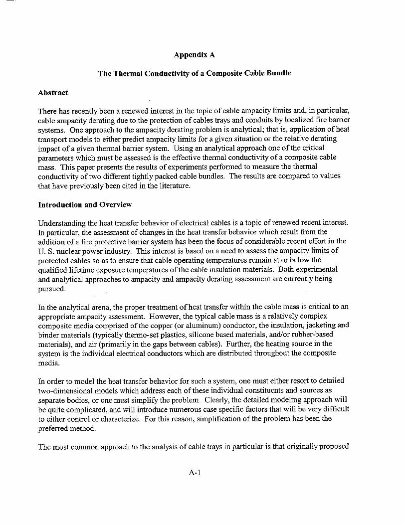
Appendix A

The Thermal Conductivity of a Composite Cable Bundle

Abstract

There has recently been a renewed interest in the topic of cable ampacity limits and, in particular, cable ampacity derating due to the protection of cables trays and conduits by localized fire barrier systems. One approach to the ampacity derating problem is analytical; that is, application of heat transport models to either predict ampacity limits for a given situation or the relative derating impact of a given thermal barrier system. Using an analytical approach one of the critical parameters which must be assessed is the effective thermal conductivity of a composite cable mass. This paper presents the results of experiments performed to measure the thermal conductivity of two different tightly packed cable bundles. The results are compared to values that have previously been cited in the literature.

Introduction and Overview

Understanding the heat transfer behavior of electrical cables is a topic of renewed recent interest. In particular, the assessment of changes in the heat transfer behavior which result from the addition of a fire protective barrier system has been the focus of considerable recent effort in the U. S. nuclear power industry. This interest is based on a need to assess the ampacity limits of protected cables so as to ensure that cable operating temperatures remain at or below the qualified lifetime exposure temperatures of the cable insulation materials. Both experimental and analytical approaches to ampacity and ampacity derating assessment are currently being pursued.

In the analytical arena, the proper treatment of heat transfer within the cable mass is critical to an appropriate ampacity assessment. However, the typical cable mass is a relatively complex composite media comprised of the copper (or aluminum) conductor, the insulation, jacketing and binder materials (typically thermo-set plastics, silicone based materials, and/or rubber-based materials), and air (primarily in the gaps between cables). Further, the heating source in the system is the individual electrical conductors which are distributed throughout the composite media.

In order to model the heat transfer behavior for such a system, one must either resort to detailed two-dimensional models which address each of these individual constituents and sources as separate bodies, or one must simplify the problem. Clearly, the detailed modeling approach will be quite complicated, and will introduce numerous case specific factors that will be very difficult to either control or characterize. For this reason, simplification of the problem has been the preferred method.

The most common approach to the analysis of cable trays in particular is that originally proposed

A-1

by Stolpe [ 1 ]. Stolpe treated the cables as an equivalent homogeneous thermal mass with uniformly distributed heat generation. He further reduced the problem to a simple onedimensional heat transfer problem by neglecting heat transfer from the sides of the cable tray. This treatment was ultimately used to develop ICEA ampacity tables for open top cable trays [2], and has also been applied in more modem applications as well. Indeed, even in recently published works on cable load diversity [3,4], variations of the Stolpe model are still applied.

Under this approach, one of the critical parameters is the equivalent thermal conductivity of the composite cable mass. The equivalent thermal conductivity plays an important role in determination of both the location and magnitude of the thermal "hot-spot." The hot-spot is of primary interest because it represents the worst-case cable operating condition. The value chosen also impacts the absolute cable ampacity limits predicted by a thermal model and, to a lesser extent, predictions of the relative impact of a fire barrier system on those ampacity limits. However, we have been unable to determine the basis for the values assumed in previously published studies including Stolpe's work [1].

This paper presents the results of two tests performed by Sandia National Laboratories (SNL) to determine the equivalent thermal conductivity for two different tightly packed cable bundles. Transient heat transfer tests in a cylindrical geometry were used as the basis for the conductivity measurement. The results provide a firm technical basis for thermal analysis of a composite cable bundle that has previously been lacking.

Experimental Approach

The basic technique used in these experiments is known by various names and has been discussed thoroughly by Drotning and Tourmey [5]. Common names include the Van de Held method, the Stalhane Pyk method, and the d'Eustacio probe method. Fundamentally, the technique is based on monitoring the transient temperature response of a line heat source (or heat probe) immersed in an infinite homogenous medium. When constant power is supplied to the probe, the temperature rise of the probe itself is a function of the thermal conductivity of the surrounding material. Numerous analyses have been performed for this arrangement, the simplest being given by Carslaw and Jeager [6]. For a probe of perfect conductance, without contact resistance, and ignoring higher order terms in the solution, the thermal conductivity of the surrounding medium is given by:

k q( 1n(t2/tl)) (A-l) k •4--(02 _ 01)

or

1 4 7 ln 0t2-- 0 1 ---lnAt-2

A-2

where (k) is the thermal conductivity of the tested medium (W/m/IK), (q) is the probe power per unit length (W/m), (t) is the time (in seconds), and (0) is the temperature ('K). The subscripts 1 and 2 refer to "arbitrary" choices of two time-temperature data pairs. In effect, this equation suggests that conductivity is inversely proportional to the slope of the time-temperature curve when plotted on a log-normal scale.

While the medium of interest in the current study is not homogeneous, the intent is to provide an equivalent composite thermal conductivity. Given this understanding, the non-homogeneous nature of the cable mass is not of fundamental concern. Also, by necessity test specimens will be of limited size rather than of infinite extent. However, the data analysis routinely performed for such tests includes a check for indications of size effects. That is, if the heat penetrates to the outer surface of the test sample (in this case the cable mass) in any significant quantity, then this would be reflected in the data as a change in the time-temperature curve slope. These and other issues associated with the non-ideal conditions of a real experiment have been explored by Drotning and Tormey [5]. The tests performed here did conform to the applicable experimental constraints as recommended in the paper by Drotning and Tormey.

Test Specimen Construction

Two test specimens were constructed for use in these experiments. In each case, the test specimen was constructed around a centrally located resistance heating probe measuring approximately 3/4" in diameter by 36" long. Lengths of the cable of interest were cut to 36" and secured to the test specimen so as to completely surround this heater probe. In particular, cables were added in concentric ring layers such that a tight cable-to-cable spacing was achieved. Each progressive ring of cables was secured to the specimen using 24 ga stainless steel wires. The wires were typically spaced at 8-12" intervals along the length of the specimen. These wire ties were also offset between adjacent cable layers. A total of six cable layers were installed for each of the two test specimens. The general sample configuration and the individual cable properties are illustrated in Figure 1.

Each of the tested bundles represents a tightly packed cable mass with minimal air gaps and no passages to support air flow through the bundle. As pointed out by Harshe and Black [3] the presence of open passages for air flow through a cable mass would promote more efficient heat transfer. This behavior could be modeled as an increase in the effective thermal conductivity of the cable mass. However, there is currently no data available to support such a treatment, and the tests described here do not address this condition.

Two types of cable were investigated. The first was an 8AWG single conductor, 600V cable with a 35 mil (0.035") polyvinyl-chloride (PVC) insulation and a 5 mil cross-linked polyethylene (XLPE) outer sheath. The second cable was a 3-conductor, 12AWG, 600V cable with a 30 mil XLPE insulation on each conductor and with a 60 mil chloro-sulfonated polyethylene (CSPE or Hypalon) over-jacket. The multi-conductor 12AWG cable also included nylon strands and a nylon sheath used as binding/filler materials in the gaps between the individual conductors and

A-3

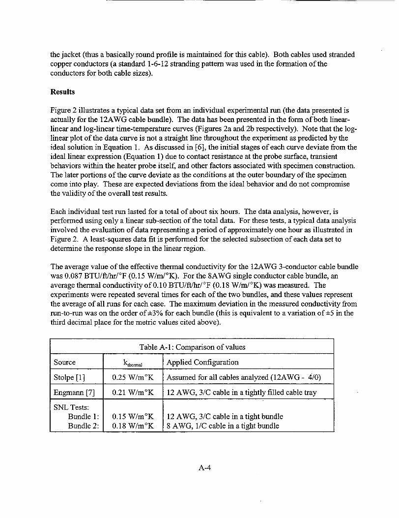
the jacket (thus a basically round profile is maintained for this cable). Both cables used stranded copper conductors (a standard 1-6-12 stranding pattern was used in the formation of the conductors for both cable sizes).

Results

Figure 2 illustrates a typical data set from an individual experimental run (the data presented is actually for the 12AWG cable bundle). The data has been presented in the form of both linearlinear and log-linear time-temperature curves (Figures 2a and 2b respectively). Note that the loglinear plot of the data curve is not a straight line throughout the experiment as predicted by the ideal solution in Equation 1. As discussed in [6], the initial stages of each curve deviate from the ideal linear expression (Equation 1) due to contact resistance at the probe surface, transient behaviors within the heater probe itself, and other factors associated with specimen construction. The later portions of the curve deviate as the conditions at the outer boundary of the specimen come into play. These are expected deviations from the ideal behavior and do not compromise the validity of the overall test results.

Each individual test run lasted for a total of about six hours. The data analysis, however, is performed using only a linear sub-section of the total data. For these tests, a typical data analysis involved the evaluation of data representing a period of approximately one hour as illustrated in Figure 2. A least-squares data fit is performed for the selected subsection of each data set to determine the response slope in the linear region.

The average value of the effective thermal conductivity for the 12AWG 3-conductor cable bundle was 0.087 BTU/ft/hr/°F (0.15 W/m/°K). For the 8AWG single conductor cable bundle, an average thermal conductivity of 0.10 BTU/ft/hr/°F (0.18 W/m/°K) was measured. The experiments were repeated several times for each of the two bundles, and these values represent the average of all runs for each case. The maximum deviation in the measured conductivity from run-to-run was on the order of ±3% for each bundle (this is equivalent to a variation of +5 in the third decimal place for the metric values cited above).

Table A-i: Comparison of values

A-4

Source kthemal Applied Configuration

Stolpe [1] 0.25 W/m°K Assumed for all cables analyzed (12AWG - 4/0)

Engmann [7] 0.21 W/m°K 12 AWG, 3/C cable in a tightly filled cable tray

SNL Tests: Bundle 1: 0.15 W/m°K 12 AWG, 3/C cable in a tight bundle Bundle 2: 0.18 W/m°K 8 AWG, 1/C cable in a tight bundle

Comparison to Previously Published Values

In a review of analytical ampacity studies two unique values of the assumed thermal conductivity of a composite cable mass region were identified as summarized in Table A-1. Stolpe [1] used a value of 0.15 BTU/ft/hr/°F (0.25 W/m/°K). (Note that the Stolpe value is originally, and typically, cited as a thermal resistivity of 400 cm-°C/W.) Engmann [7] used a value of 0.12 BTU/ft/hr/°F (0.21 W/m/°K). The basis for these values was not provided by either author. All of the other identified tray modeling papers [3,4,8-11] were found to have cited one or both of these papers as the source of the assumed conductivity. As summarized in Table A-I, both of the values found in the SNL tests are considerably lower than those assumed by Stolpe and by Engrann.

Recall that Fourier's Law states that the heat flux in steady state conduction is directly proportional to the temperature gradient (dT/dx), with thermal conductivity (k) being the proportionality constant. Hence, the impact of a reduced thermal conductivity would be the relative "slowing" of heat transfer rates within the cable mass; or as an alternate view, a reduction in thermal conductivity would result in higher temperature gradients required to support a given level of heat transfer. The primary effect of such a change would be to increase the hot-spot temperature for a given ampacity (heat load) in the cable bundle; or alternatively, to reduce the allowable ampacity for a given hot-spot temperature.

In the end, Stolpe obtained excellent agreement between his calculations and experiments. The current test results would indicate that his use of a relatively high thermal conductivity value may, in fact, have offset to at least some extent other sources of conservatism in his original ampacity calculations. In particular, Stolpe applied convection correlations that are somewhat pessimistic in comparison to accepted modem correlations, and gave no credit to heat transfer from the sides of the tray.

When the analytical application involves estimating the relative fire barrier ampacity derating impact, a reduced thermal conductivity would impact both the baseline (unprotected) and clad (protected) condition analyses. Hence, the impact of conductivity changes on predicted fire barrier ampacity correction factor (ACF, the ratio of the clad to baseline ampacity) is more difficult to assess, but is also expected to be more modest. To a large extent the impact of such a change is offset by the fact that the "final answer," ACF, is the ratio of two ampacity values, both of which are impacted by the change in thermal conductivity.

In limited applications explored by SNL, a reduction in the cable mass thermal conductivity with no other modeling changes generally resulted in a modest decrease in the derating penalty predicted (i.e., a slightly higher ACF value). It would appear that the change has a more pronounced effect on the baseline case than it does on the clad case. This is consistent with expectations because confined space convection (between the cables and the inside surface of the barrier system) plays a comparatively more dominant role in the analysis of the clad case than does external convection in the baseline case. Hence, the role of cable conduction in the clad

A-5

case is comparatively less significant.

A second effect of note for these applications is that a reduced conductivity also shifts the location of the hot-spot within the cable mass. The hot-spot is that location within the cable mass where the maximum operating temperature is encountered. This location is of particular importance because it represents the worse-case operating condition for the system as a whole. In general, because the upper surfaces are more effective at heat transfer (due to buoyancy induced convective enhancement), the location of the hot-spot would be expected to shift downward within the cable mass with decreasing conductivity. This would maintain the overall upward/downward conduction/convection balance.

Prior to the performance of these tests, SNL undertook an effort to review past cable tray ampacity modeling efforts. As a part this review a simple cable tray thermal model was assembled based largely on earlier published efforts. (See Appendix F of this report for a description of the SNL Cable Tray Thermal Model.) Those aspects of each of the earlier models considered "best" were consolidated into an improved thermal model for the simulation of cable tray fire barrier ampacity effects.' With a cable tray fire barrier, one basically builds a protective envelope around the tray to protect the cables from the damaging effects of a fire. The materials available vary widely, but all introduce some ampacity penalty due to the isolation of the cables within an enclosed air pocket, and the inevitable insulating effect of the surrounding barrier material. In some cases the ampacity penalty can be substantial; resulting in a 50% reduction in the allowable ampacity limits or worse. Based on attempts to thermally model this problem, some interesting insights were developed.

Of particular relevance to the current discussion, as a part of the SNL efforts the sensitivity of the thermal model to selected input parameters was explored. This exercise did illustrate that the models were sensitive to the assumed valued of cable mass thermal conductivity. As noted above, the basis for the values cited in the literature was not established, and this was considered the one parameter in the model input with the greatest potential uncertainty. Hence, values of this parameter were explored in an attempt to better match certain experimental data on actual measured clad and unprotected cable tray ampacities [ 12]. It was found that reducing the assumed value of the cable region thermal conductivity from the values cited in the literature (0.12-0.15 BTU/ft/hr/°F) to a value of 0.08 BTU/ft/hr/0 F (0.14 W/m/0 K) produced the best matches to the experimental data, including both the cable hot-spot and intermediate temperatures (cable surface, barrier inner temperature, barrier outer temperature). It is now interesting to note that these earlier modeling efforts led us to a thermal conductivity value that is quite consistent with the value determined in the later experiments for a 3-conductor 12AWG cable, namely, 0.087BTU/ft/hr/°F (0.15 W/m°/K). This is quite encouraging in light of the fact that the same type of cable was also used in the ampacity experiments being simulated, a 3

'These efforts are documented in an unpublished SNL Letter Report entitled "Fire Barrier Ampacity Derating: A Review of Experimental and Analytical Studies," August 25, 1995. The report is available through the USNRC public document room.

A-6

conductor 12AWG cable, although the exact composition of the cable insulation materials is unknown.

Summary

Tests were performed to measure the equivalent thermal conductivity for two different tightly packed cable bundles. For a bundle of 3-conductor, 12AWG, 600V, XLPE/CSPE cables a conductivity of 0.087 BTU/ftihr/°F (0.15 W/m/IK) was measured. For a bundle of single conductor, 8AWG, 600V, PVC/XLPE cables, a thermal conductivity of 0.10 BTU/ft/hr/°F (0.18 W/m/°K) was measured. Each value was found to be repeatable to within ±3%.

These values were compared to those cited in previously published analytical studies of cable tray heat transfer behavior. In particular Stolpe [1] used a value of 0.15 BTU/ft/hr/°F (0.25 W/m/IK) and Engmann [4] used a value of 0.12 BTU/ftlhr/0F (0.21 W/mi°K). Other published works have typically cited one or both of these studies as the basis for their assumed thermal conductivity. In Stolpe the value was assumed for all of the cables tested, ranging from 12 AWG up to #4/0. Given the larger cables tested by Stolpe and the resulting increase in the relative copper content, a higher average conductivity for all of the cable tested would be expected. In Engmann [4] the values were assumed for cables nominally similar to the 3-conductor 12AWG cable tested by SNL. The SNL determined values are substantially lower than those assumed in these previous studies. As used in most simple cable tray thermal models, the net effect of a reduction in cable mass thermal conductivity would be a decrease in the predicted absolute ampacity limits for a given cable arrangement.

The tests do not, however, consider the effects of a looser cable packing. As suggested by Harshe and Black [3], such behavior might be modeled by simply assuming a higher effective thermal conductivity in the cable mass. This approach should be taken only with great caution however. Initially, a looser packing might actually reduce conductivity as the cable-to-cable contract resistance increases and the "air pocket fraction" increases. Once the packing is sufficiently loose to allow air to actually circulate through the mass, the effective conductivity would increase, possibly sharply. Allowing generic credit for convective enhancement due to loose cable packing will likely not be practical because many applications will involve tight cable packing and for others the packing density will be difficult to establish and maintain over time. This is, however, a potential area for future investigation that might lead to more liberal assessments of ampacity margins on a case-by-case basis under conditions that allow for strict installation control. Of particular benefit in this regard might be the investigation of maintained spacing applications with a sufficient number of cables that no ampacity benefit is gained by use of, for example, the IPCEA P-46-426 [13] maintained spacing methods as compared to the Stolpe/ICEA P- 54-440 random fill methods.

Finally, the measured values compare quite favorably to the results of certain model validation based findings that pre-dated the experiments by some months. In these prior studies, it was found that using a thermal conductivity value of 0.08 BTU/fl/hr/°F (0.14 W/mi°K) provided the

A-7

most satisfactory results when attempting to predict the absolute ampacity results measured during the testing of a 3-conductor 12AWG cable [12]. This finding is quite consistent with the measured results reported here for the 3-conductor 12AWG cable bundle.

References

1. Stolpe, J., "Ampacities for Cables in Randomly Filled Trays," IEEE Transactions on Power Apparatus and Systems, Vol. PAS-90, Pt. I, PP 962-974, 1971.

2 Ampacities of Cables in Open-Top Cable Trays, ICEA P-54-440, NEMA WC 51, 1986. 3 Harshe, B. L. and Black, W. Z., "Ampacity of Cables in Single Open-Top Cable Trays,"

IEEE Transaction on Power Delivery, Vol. 9, No. 1, pp. 1733-1739, Oct. 1994. 4 Leake, H. C., "Sizing of Cables in Randomly-Filled Trays With Consideration for Load

Diversity," IEEE Transactions on Power Delivery, paper 96 SM 372-3 PWRD, Jan. 1997. 5 Drotning, W.D. and Tormey, T.V., "Thermal Conductivity Probe Measurement System",

Sandia National Laboratories, SAND83-2057, Albuquerque, New Mexico, 1984. 6 Carslaw, H.S. and Jaeger, J.C., Conduction of Heat in Solids, 2nd Ed., Oxford Univ. Press,

Oxford, England, 1959, pp 261-262 and 341-345. 7 Engmann, G., "Ampacity of Cables in Covered Trays," IEEE Transactions on Power

Apparatus and Systems, Vol. PAS-103, No. 2, PP 345-352, Feb. 1984. 8 Save, P., and Engmann, G., "Fire Protection Wrapped Cable Tray Ampacity," IEEE

Transactions on Energy Conversion, V4, No. 4, Dec. 1989. 9 Esteves, 0. M., "Derating Cables in Trays Traversing Firestops or Wrapped in

Fireproofing," IEEE Transactions on Power Apparatus and Systems, Vol. PAS-102, No. 6, June 1983.

10. Lee, R.H., "Ampacities of Multiconductor Cables in Trays," IEEE T-PAS-1972. 11 Nemeth, C.W., et.al., "Ampacities of Cables in Trays with Firestops," IEEE Transactions on

Power Apparatus and Systems, PAS- 100, No. 7, July 1981. 12 Ampacity Derating of Fire Protected Cables - Electrical Test to Determine the Ampacity

Derating of a Protective Envelope for Class 1E Electrical Circuits, by Omega Point Laboratories for Texas Utilities Electric Co., Comanche Peak Steam Electric Station, Project No. 12340-94583,95165-95168,95246, March 19, 1993.

13. Power Cable Ampacities, IPCEA P-46-426, AIEE S-135-1, ajoint publication of the Insulated Power Cables Engineers Association (now ICEA) and the Insulated Conductors Committee Power Division of AIEE (now IEEE), 1962.

14. C. L. Choy, "Thermal conductivity of polymers," Polymer, V18:984, 1977. 15. Carlos J. Hilado, Flammability handbook for plastics, Technomic Pub., 2nd Ed., 1974.

A-8

Specimen Nominal Arrangement:

(d=0 .75")

-Heater Probe (d=0 . 75*")

/CSPE Jacket (t=0.060")

XLPE Insulation (t=o.0o30")

Cu Conductor

(d=0 .095")

Binder/Filler Materials

`d=0.45"

-XLPE Sheath (t=0.005")

'-PVC Insulation (t=0.035")

Cu Conductor

(d=0.045")

d=0. 125"

Figure 1: Nominal construction and physical characteristics of the 12 AWG 3/C cable (top) and the 8 AWG 1/C cable (bottom) bundles tested.

A-9

Cable Construction:

34

32

30 -

28

26

24 _ 22 20,

0 5000 10000 15000 20000 25000

Time (s)

(a) Data plotted on a linear-linear time-temperature graph.

34

32

30

28

26

24

22

20

1.E+02 1.E+03 1.E+04 1.E+051.E+01

Time (s)

(b) Data plotted on a log-linear time-temperature graph

Figure A-2: Typical data plot from a cable bundle thermal conductivity experiment. Data analysis in this case was based on data centered about 1x 104 seconds, the "linear" range as illustrated in (b).

A-10

0

E 0 I-

5. 0 1.=

a.'

E i-

Appendix B

The Neher and McGrath Conduit Model

Introduction

The Neher-McGrath method for the analysis of conduit ampacity was published in 1957 and still

finds wide use today. The original paper is quite complete and covers a number of topics that go

well beyond the question of cable ampacity for cables in conduit. This appendix will focus only

on the method as applied to conduit ampacity assessments. The intent is not to fully reproduce

the original work, but rather, to distill the original paper down to the critical elements applicable to a modem conduit application ampacity assessment. The discussions here also provide some

cautions regarding the application of the method and potential areas of mis-interpretation.

A Note on Units

The units used in the original work by Neher-McGrath are both mixed and somewhat unusual in

comparison to common units of modem heat transfer. For one, the original work refers to a materials thermal resistivity (p1). It is more common today to refer to a materials thermal conductivity (k.). In this case, the two are simply the inverse of each other:

1 P i --

ki

A second case is the units used to express thermal resistance. In modem applications one

commonly uses units of W/m'" C to express thermal conductivity. Thermal resistance is simply

the inverse of this (°C-m 2/W). Neher-McGrath refer to this same group of thermal resistance units as a "thermal ohm." They often refer to resistance values as "thermal ohm-feet" which is

simply the inverse of thermal conductivity per unit foot of length or the thermal resistance over a foot of system (conduit) length.

Another factor to watch carefully is the mixing of metric and English units. Most of the units

used are metric, but there are exceptions. For example, cable and conduit diameters are expressed in inches, and all assessments are made for a unit foot length of raceway. Hence, for example, conductor resistance must be expressed in units of ohms/ft, and thermal resistance terms are expressed in units of thermal ohm-feet. Great care must be exercised to ensure that a consistent units set is applied, consistent in this context being consistent with the original variable definitions. Also note that several of the expressions include numerical and empirical

constants (see examples below). While these constants are presented as nominally non

dimensional, each in fact does have implied units. Other variables in each expression must be

defined in units consistent with the original work to maintain an overall consistency of units.

B-1

The General Approach of Neher-McGrath for Conduits

The Neher-McGrath approach is an analytical model of heat transfer that was validated by comparison to available experiments. The model as applied to conduits basically builds up a three-stage heat transfer model working from the inside-out including heat transfer within an individual insulated conductor, between an insulated conductor and the conduit including the effects of cable bundling, and between the conduit and the ambient.

The most general form of the model includes terms to account for both resistance heating in the conductors and inductive heating effects in the cable sheath and/or the conduit itself. However, in practical applications the inductive heating effects can generally be neglected. Hence, for simplicity this discussion shall assume that all of the heat in the system is being generated within the cable conductors themselves.' Also, we follow through with a notation change that is not well documented in the original paper.2 With this simplification, the overall thermal model is expressed by the following equation:

AT: = W,(R, + RSd + Re)

where:

ATc Temperature rise from the ambient to the conductor

Wc Heat generation per unit length per conductor

R. Thermal resistance of each conductor's insulation 1

Rd Thermal resistance between each insulated conductor and the conduit

Re =_ Thermal resistance between conduit and ambient

In this expression it is important to note that Neher-McGrath define the heat generation rate (We) as the heat generated per unit length of conductor. That is, W, is the heating rate for a single conductor rather than the total heat for all conductors in the conduit. This approach is necessary in order to capture both individual conductor and cable bundle behavior in a single expression. The term R, is associated with thermal resistance in the insulation of each insulated conductor, so the temperature rise in that element of the model is based on the individual conductor's heating rate (We). However, the terms R~d and R, relate to the system of cables as a whole and hence, the appropriate heat load is the total heat load for all conductors within the conduit. As will be seen

'This is equivalent to setting q, and q, to unity (1.0) in Neher-McGrath equation 2.

2Equation 2 in the original work contains the factor Re, which is cited as the resistance between the cable sheath and conduit. For more general applications this term is substituted by Red which is the thermal resistance between the surface of an insulated conductor and the surrounding enclosure or conduit. For simplicity of presentation, we will go ahead an make this substitution immediately.

B-2

below, the expressions for calculating the latter two terms each include a factor (n') to account for the total number or conductors in the conduit. The implied product terms (Rsd*W,) and (Re*W,) therefore inherently include in them the internal product (n'*W,) which is the total heat load for all of the conductors. Hence, when fully executed the equation is self consistent. This subtlety is, however, easily overlooked or mis-understood, and must be carefully observed.

The conductor heating rate W, is given significant treatment in the paper. Included is the consideration of load factors, inductive heating, a-c versus d-c current, and the impact of temperature on conductor resistance. Ultimately, in most practical applications this all can be boiled down to simple resistance heating within each individual conductor as follows:

W, = I 2R

where I is the current in the conductor and R is the resistance per foot of conductor taken at the desired final conductor temperature (typically 90'C) and as applicable to either a-c or d-c current flow.

The thermal resistance of each individual conductor's insulation is given by the common expression for heat flow in an annular ring as follows:

Ri = 0.01__2 log Dti kc Do

where kc is the thermal conductivity of the insulation material, Di is the diameter of the conductor (or inner diameter of the insulation layer) and DO is the outer diameter of the insulation. Note that for a single conductor cable with a jacket or any conductor with an individual jacket, the outer diameter should include the jacket layer as well.

The remaining two factors, R~d and Re are the subject of some considerable development in the original work. The cable to conduit thermal resistance term, R~d, is intended to address several individual effects. First, for any cable the heat transfer geometry between the cable and conduit is complex and non-symmetric. There is some partial direct contact, internal convection, and internal radiation to be accounted for. In addition, Rd also accounts for the thermal effects of both multi-conductor cables and bundling of multiple cables within a conduit. The development of RSd is actually documented in an earlier work by Buller and NeherP21 and is based on a combined theoretical and empirical development supplemented by extensive experimental validation. The same factor is expressed in three primary forms, all of which are roughly equivalent for common applications. Each progressive form introduces assumptions and restrictions on its applicability that can be used to simplify the expression. The most general form for RSd in thermal ohm-feet is:

B-3

d D a T /4 + b + cTm1

where T is the temperature difference between the cable surface and the conduit (0C), P is the absolute pressure of the air (atmospheres), Tm is the mean temperature of the intervening medium (in this case the air in the conduit, (QC)), and n' is the total number of conductors within the conduit (not the number of cables, nor the number of conductors per cable, but the total conductor count). The factors a, b, and c are empirical constants. For cables in a metallic conduit the recommended values are (a=0.07), (b=0.121), and (c=0.0017). The factor D,' is the effective cable bundle diameter (inches) and is calculated as follows:

1 cable - Ds'= 1.00 * Dcable

2 cables - D= 1.65 * Dcable

3 cables - D ' 2.15 *Dcabl, 4 cables - D= 2.50 * Dcable

For most cases it is not necessary to revert to this most general expression. To simplify the expression, several assumptions regarding a typical condition can be made. If one assumes a pressure of 1 atmosphere, and a typical cable-to-conduit temperature drop of 20 'C (this value was based on the experiments performed during validation of the method) then the equation can be simplified somewhat. Note that the temperature difference in particular appears as a 1/4 power term in the general expression, so the dependency on this value is rather weak. If one further restricts the equation to cases involving an effective cable diameter between 1 and 4 inches (for cables in a conduit), then a simplified expression is of the following form is obtained:

Rsd = n tWA 1+(B+CTm)D,'

where A, B, and C are a new set of empirical constants. For cables in a metallic conduit the recommended values are (A= 7), (B=3.6), and (C=0.029). This particular expression eliminates the need for an iterative solution (i.e., one where the cable surface and conduit temperatures must be matched to the thermal resistance and heat flow in an iterative manner).

This expression can be further simplified if one assumes that the typical value of Tm is 60'C. In this case the third and most simplistic form is obtained as follows:

n'A' RSd = DS +B'

B-4

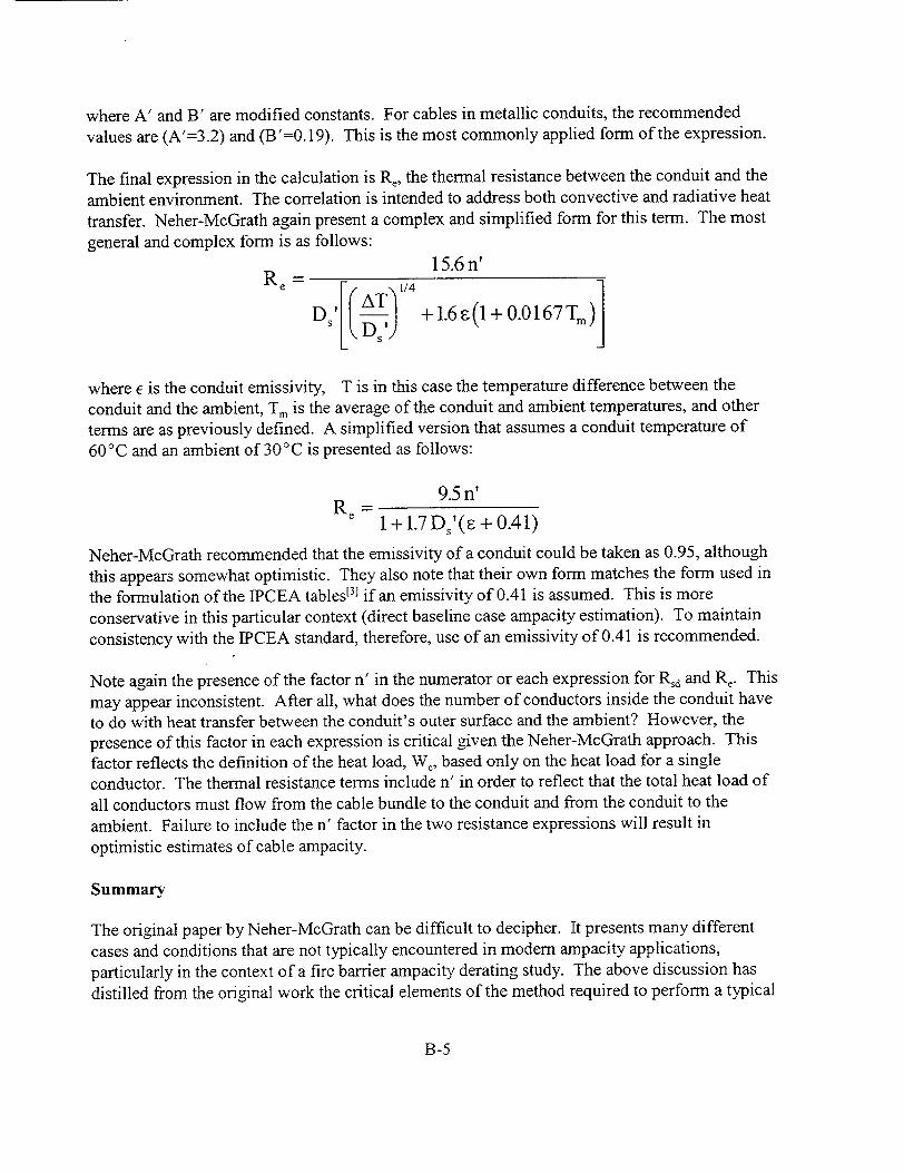
where A' and B' are modified constants. For cables in metallic conduits, the recommended values are (A'=3.2) and (B'=0.19). This is the most commonly applied form of the expression.

The final expression in the calculation is Re, the thermal resistance between the conduit and the

ambient environment. The correlation is intended to address both convective and radiative heat

transfer. Neher-McGrath again present a complex and simplified form for this term. The most general and complex form is as follows:

15.6 n' Re =1/4

DS1r TD +1.6F(1+0.0167Tm)

where c is the conduit emissivity, T is in this case the temperature difference between the

conduit and the ambient, Tm is the average of the conduit and ambient temperatures, and other terms are as previously defined. A simplified version that assumes a conduit temperature of

60'C and an ambient of 30'C is presented as follows:

9.5n' e 1 + 1.7 DA'(• + 0.41)

Neher-McGrath recommended that the emissivity of a conduit could be taken as 0.95, although this appears somewhat optimistic. They also note that their own form matches the form used in

the formulation of the IPCEA tables131 if an emissivity of 0.41 is assumed. This is more conservative in this particular context (direct baseline case ampacity estimation). To maintain consistency with the IPCEA standard, therefore, use of an emissivity of 0.41 is recommended.

Note again the presence of the factor n' in the numerator or each expression for Rld and Re. This may appear inconsistent. After all, what does the number of conductors inside the conduit have to do with heat transfer between the conduit's outer surface and the ambient? However, the presence of this factor in each expression is critical given the Neher-McGrath approach. This factor reflects the definition of the heat load, Wc, based only on the heat load for a single conductor. The thermal resistance terms include n' in order to reflect that the total heat load of all conductors must flow from the cable bundle to the conduit and from the conduit to the ambient. Failure to include the n' factor in the two resistance expressions will result in optimistic estimates of cable ampacity.

Summary

The original paper by Neher-McGrath can be difficult to decipher. It presents many different

cases and conditions that are not typically encountered in modem ampacity applications, particularly in the context of a fire barrier ampacity derating study. The above discussion has distilled from the original work the critical elements of the method required to perform a typical

B-5

conduit ampacity assessment. In doing this we have neglected such effects as inductive heating, and have moved directly to those equations and formulations relevant to the conduit problem.

B-6

Appendix C

The Stolpe/ICEA Cable Tray Model

Introduction

Note that the objective of this section is to provide the reader with an overview of the Stolpe/ICEA cable tray ampacity model. It is not intended that this discussion will cover all aspects of the model, but rather, that the reader will be familiarized with the modeling approach and objectives, and will be provided with practical guidance on the application of the model to actual cable trays. The reader should refer to the appropriate source references for additional detail if that is required. Both publications remain readily available.

Stolpe's original work on ampacity for cable trays was published in 1970. This approach was ultimately adopted in the ICEA P-54-440 standard "Ampacities of cables in Open-Top Cable Trays." There are modest differences between Stolpe's original work and the ICEA standard that do not impact the final results of the model, but do require some care to ensure one is consistent in the treatment. The model as discussed here is consistent with the ICEA approach. The point of difference is in relation to defining the cable cross-section and tray depth of fill and will be highlighted in the text below.

Modeling Approach

The general approach to modeling employs a simple one-dimensional, steady state model of heat transfer in a cable tray. To achieve this, the model makes four critical simplifying assumptions:

Heat transfer from the sides of the tray are neglected. This eliminates the two dimensional effects that would be present near the sides of the tray. This is also one source of conservatism in Stolpe's model.

The hot spot is assumed to occur at the center of the cable mass. In reality the hot spot will generally occur below the cable mass center because convective heat transfer from the top surface will be more efficient than that from the bottom surface of the heated cables due to the fact that buoyancy is working with the top surface and against the lower surface. However, Stolpe is self-consistent in that a single composite correlation is used to characterize both the top and bottom surfaces. It might also be noted here that Stolpe used relatively pessimistic convection correlations in comparison to typically accepted modem correlations. This is a second source of conservatism in the model.

The model assumes that the cable mass can be represented by a single homogeneous region. This allows for a simplified treatment of heat conduction within the cable mass. Stolpe assumed a thermal conduction value for the cables that now appears to have been optimistic (see Appendix A). This may have offset other sources of conservatism in the

C-1

final results.

Heat generated by the cables due to resistance heating is assumed to be uniformly distributed over the entire cable mass. By implication this assumes that all cables are energized to their full rated ampacity (no diversity).

These assumptions allowed Stolpe to model conduction in the cable mass using standard steadystate solutions for heat conduction in a one-dimensional slab with uniform heat generation.

The model treats heat generation in the cable mass, internal conduction within the cable mass, and convection and radiation heat transfer to the ambient environment. The model was developed using accepted engineering correlations for each of the subject phenomena (details can be found in the source reference by Stolpe). The model was developed only for open cable trays and does not address fire barrier cladding systems. The model can be modified to include the effects of a fire barrier system, but this must be done by the individual user.

Ultimately, the objective of the model is to predict the (uniform) heat generation rate for the cable mass that yields a cable hot-spot temperature equal to the continuous operating temperature rating of the cables, typically 90'C. This is accomplished through a simple iterative process that matches the cable hot spot temperature for a given ambient temperature and fill depth. In practice, the heating rate is ultimately found to be a function of cable depth only. This is because in the standard, no adjustments are made to the heat transfer correlations nor cable properties (thermal conductivity and emissivity) to reflect a specific cable or loading configuration. Hence, the model results can be calculated once for each desired depth of fill condition, and can then be applied repeatedly to any case that matches that depth of fill. Appendix B of the standard does provide the raw heating rate results used in generating the tables.

One fallacy that is sometimes cited regarding Stolpe's model is that Stolpe did not credit convection or radiation from the lower surface of the cable tray. This is not correct - Stolpe's model did credit heat transfer from the bottom surface of the tray, both radiation and convection. Any direct implementation of the model will reveal this to be true. That is, one cannot match either Stolpe's results nor those of the ICEA standard without crediting both the top and bottom surfaces. This perception typically arises because in his experiments Stolpe used a plastic sheet to cover the bottom of the tray. This was not, however, done to limit the heat transfer from the bottom surface as is often perceived. Rather, this was done to limit the flow of air up and through the cable mass in his trays.

This heat generation rate, expressed commonly in W/ft/in2 of cable cross-section, is then partitioned to individual cables in accordance with their contribution to the total cable crosssectional area. That is, a cable whose cross-section represents 5% of the total cable mass crosssection will be allocated 5% of the total heat load predicted by the model. In practice, one calculates the cables cross-section in square-inches, and multiplies this value by the heating rate

C-2

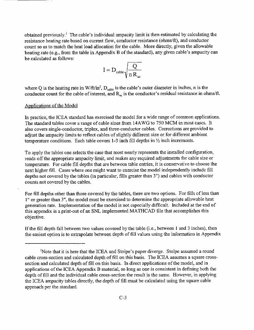
obtained previously.' The cable's individual ampacity limit is then estimated by calculating the resistance heating rate based on current flow, conductor resistance (ohms/ft), and conductor count so as to match the heat load allocation for the cable. More directly, given the allowable heating rate (e.g., from the table in Appendix B of the standard), any given cable's ampacity can be calculated as follows:

I=Dcable n R

where Q is the heating rate in W/ft/in2, D~ble is the cable's outer diameter in inches, n is the conductor count for the cable of interest, and R,, is the conductor's residual resistance in ohms/ft.

Applications of the Model

In practice, the ICEA standard has exercised the model for a wide range of common applications. The standard tables cover a range of cable sizes from 14AWG to 750 MCM in most cases. It also covers single-conductor, triplex, and three-conductor cables. Corrections are provided to adjust the ampacity limits to reflect cables of slightly different size or for different ambient temperature conditions. Each table covers 1-3 inch fill depths in V2 inch increments.

To apply the tables one selects the case that most nearly represents the installed configuration, reads off the appropriate ampacity limit, and makes any required adjustments for cable size or temperature. For cable fill depths that are between table entries, it is conservative to choose the next higher fill. Cases where one might want to exercise the model independently include fill depths not covered by the tables (in particular, fills greater than 3") and cables with conductor counts not covered by the cables.

For fill depths other than those covered by the tables, there are two options. For fills of less than 1" or greater than 3", the model must be exercised to determine the appropriate allowable heat generation rate. Implementation of the model is not especially difficult. Included at the end of this appendix is a print-out of an SNL implemented MATHCAD file that accomplishes this objective.

If the fill depth fall between two values covered by the table (i.e., between 1 and 3 inches), then the easiest option is to extrapolate between depth of fill values using the information in Appendix

'Note that it is here that the ICEA and Stolpe's paper diverge. Stolpe assumed a round cable cross-section and calculated depth of fill on this basis. The ICEA assumes a square crosssection and calculated depth of fill on this basis. In direct applications of the model, and in applications of the ICEA Appendix B material, so long as one is consistent in defining both the depth of fill and the individual cable cross-section the result is the same. However, in applying the ICEA ampacity tables directly, the depth of fill must be calculated using the square cable approach per the standard.

C-3

B of the standard. Stolpe demonstrated that the heating rate versus depth of fill was nearly linear when plotted on a log-log scale. Hence, extrapolation using a logarithmic expression is appropriate. SNL has worked out a set of extrapolation factors for use in this approach. The basic extrapolation formula is as follows:

Q = 10B. dfi

where Q is the allowable heating length given in W/ft/in2, d4 is the fill depth in inches, and the factors B and A are constants that have been derived for each applicable fill range. The recommended values are summarized in Table B-I below. Note that extrapolating outside the specific ranges (below 1" or above 3") will provide an approximately correct answer, but such extrapolations should be verified by direct modeling.

Table B-i: Recommended extrapolation factors for intermediate tray fill depths.

MATHCAD Implementation

The following provides a simple SNL created MATHCAD file that implements the Stolpe/ICEA thermal model. The user is required to specify the desired fill depth and can also alter the assumed ambient and cable temperature conditions. One can also change the tray width, but this has very little impact on the model results (a minor impact on the convection correlation is realized). The calculation provides both the allowable heating rate for the tray (consistent with the table in ICEA P-54-440, Appendix B) and can be used to estimate the actual ampacity for any given cable as well.

A comment on MATHCAD: MATHCAD is a symbolic mathematics package that automatically recognizes and converts units into self-consistent sets. Units are specified in the definition of a constant or seed parameter, but are then converted as need when the variable is used in a subsequent expression. However, one must recognize that early version of MATHCAD did not provide default temperature units. The SNL implementation is based on MATHCAD version 8. This version does provide temperature units directly (degrees-Kelvin). For earlier versions of the program consult the program documentation for guidance on how the user can "redefine" an unused default unit (typically coulombs works well) to utilize as a surrogate for temperature units.

C-4

Depth of fill range B 10 A

1" < df11 < 1.5" 0.7727 5.925 -1.258

1.5" < dfil < 2" 0.7851 6.096 -1.329

2" < dfil < 2.5" 0.8003 6.314 -1.379

2.5" < dfil < 3" 0.8165 6.553 -1.420

This file provides a simple implementation of the Stolpe Model for cable trays. The model yeilds the results in terms of the allowable heat generation rate per foot of cable tray length as in Appendix B of the ICEA P-54-440 standard. The file can be used to find ampacity values for any depth of fill consistent with the standard.

Temperature conversion for convienience:

CtoK:= 273.16.K

Stefan Boltzmann constant:

S :=5.669.10 O 8. 2.4

m K

Values predefined by the Stolpe/ICEA method:

6 cable:` 0.8

W k:= 0.25.

mnKCable Mass Thermal Conductivity

User Input:

T hotspot:= 90.K + CtoK

T ambient:40K + CtoK

d:= 2.in

w:= 24.in

cable hot spot temperature

Ambient temperature

Tray depth of fill

Tray width

Derived constants based on user input:

A := 2-w Cable surface area per unit foot of tray length!

Must provide seed values for each unknown to initiate the solve block below:

W h:= 5.-

f2.K

W Q total:= 5-

ft

T surface:= 80. K + CtoK

Convection coefficient

Note that Q is heat per unit foot of tray lengtl"

Surface temperature

C-5

Solve block for answer (three equations and three unknowns to solve):

Given

h= 0.223.[ (T surface- T ambiený 10.25 7W w'l-K f?•--.K

C 4 T 4\

Qtotah.A s" (T surface- T ambien4 + a cable.A s T surface- T(bient)

d T surface= T hotspot - Q total k. 8w

T surface

Q total Find(T surface, Q total, h)

h

The answer is:

T surface- CtoK = 80.296 KW

h = 0.254ft2*K

Q total= 141.972 o ft

Normalized to unit tray length and per square inch of cable cross-section:

Q total Q area:= Qo

w.d

W Q area = 2.423 2

ft. in

Convert to heat per unit cross-section per unit foot of tray length

This value should match the ICEA table in

Appendix B for a depth of fill of:

d = 2 oin

C-6

To turn this into a cable ampacity you must specify the following additional factors:

(Example is a 3-conductor 12AWG cable per Table 3-6 of the standard)

d cable:= 0.49.in cable outside diameter

r cable :=2-07.ohm Conductor resistance

1000.ft

n conductors: 3 Number of conductors in cable

Now we calculate ampacity as follows: A cable = d cabl2 Standard uses square cables for both fill depth and

cross-section of a given cable!!

Q cable:= Q area"A cable Heat load alloaction for our cable based on area!

Q cable 0.5 Cacluclate ampacity to match the heat load cable allocation ( = n * 1A2 * r) based on resistance

ln conductors-r cable heating.

So the final answer for our sample case is:

I cable = 9.678 A Note that the table will round down!

C-7

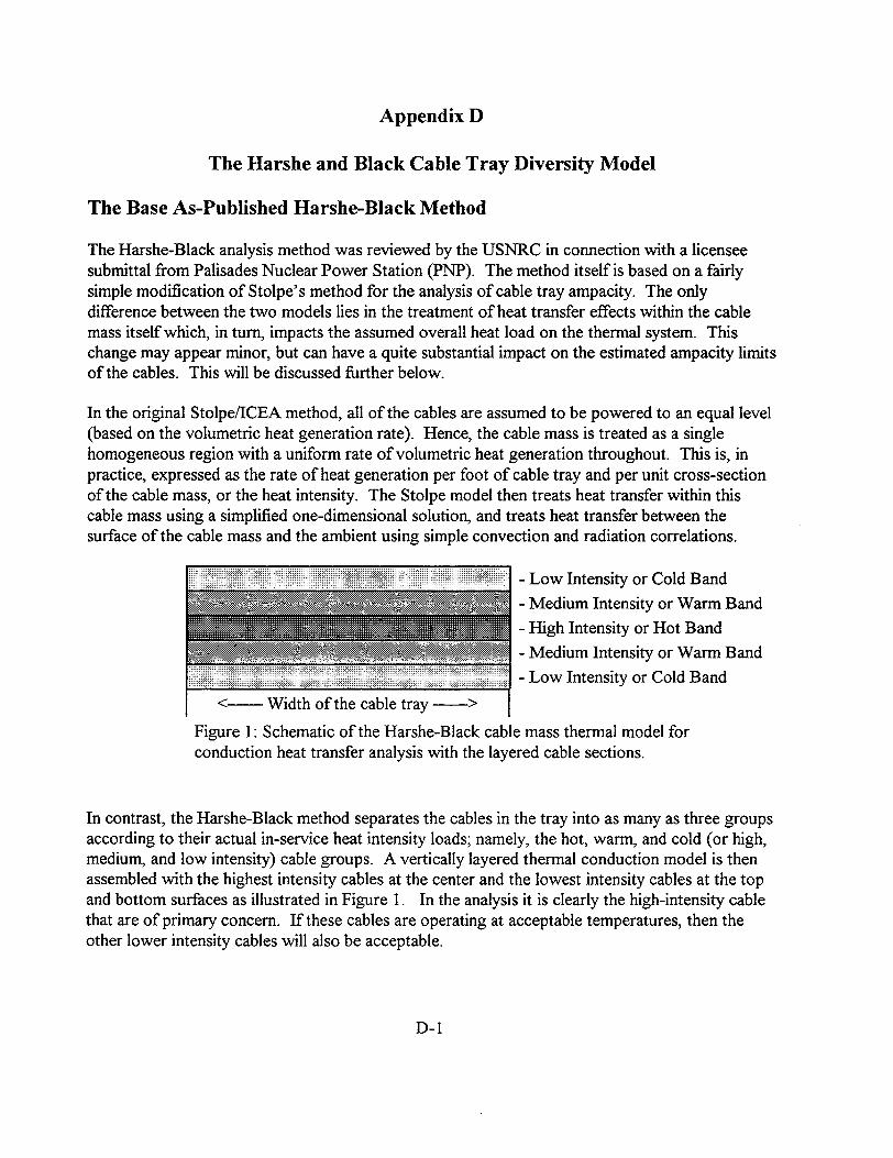
Appendix D

The Harshe and Black Cable Tray Diversity Model

The Base As-Published Harshe-Black Method

The Harshe-Black analysis method was reviewed by the USNRC in connection with a licensee submittal from Palisades Nuclear Power Station (PNP). The method itself is based on a fairly simple modification of Stolpe's method for the analysis of cable tray ampacity. The only difference between the two models lies in the treatment of heat transfer effects within the cable mass itself which, in turn, impacts the assumed overall heat load on the thermal system. This change may appear minor, but can have a quite substantial impact on the estimated ampacity limits of the cables. This will be discussed further below.

In the original Stolpe/ICEA method, all of the cables are assumed to be powered to an equal level (based on the volumetric heat generation rate). Hence, the cable mass is treated as a single homogeneous region with a uniform rate of volumetric heat generation throughout. This is, in practice, expressed as the rate of heat generation per foot of cable tray and per unit cross-section of the cable mass, or the heat intensity. The Stolpe model then treats heat transfer within this cable mass using a simplified one-dimensional solution, and treats heat transfer between the surface of the cable mass and the ambient using simple convection and radiation correlations.

- Low Intensity or Cold Band

ON. Medium Intensity or Warm Band - High Intensity or Hot Band

Ilk 010 "N.: -Medium Intensity or Warm Band - Low Intensity or Cold Band

<---- Width of the cable tray ->

Figure 1: Schematic of the Harshe-Black cable mass thermal model for conduction heat transfer analysis with the layered cable sections.

In contrast, the Harshe-Black method separates the cables in the tray into as many as three groups according to their actual in-service heat intensity loads; namely, the hot, warm, and cold (or high, medium, and low intensity) cable groups. A vertically layered thermal conduction model is then assembled with the highest intensity cables at the center and the lowest intensity cables at the top and bottom surfaces as illustrated in Figure 1. In the analysis it is clearly the high-intensity cable that are of primary concern. If these cables are operating at acceptable temperatures, then the other lower intensity cables will also be acceptable.

D-1

One specific aspect of this change is also very important. That is, the heat generation rate for each layer is based on the sum of the actual heating rates for the individual cables in that group. This is will substantially reduce the overall system heat load in comparison to the Stolpe model in which all cables are assumed to be powered to their allowable ampacity limit.

The overall thermal model is based on a conduction analysis of the layered cable mass coupled with a standard treatment of the cable surface to ambient convection and radiation behavior. Significant increases in the estimated allowable ampacity limits are realized because (1) the zone of highest heating is limited in size as compared to Stolpe's model, and (2) the overall heat load on the system is reduced compared to Stolpe. Both factors contribute to lower temperature drops for a given situation, or equivalently, higher maximum heat intensity limits for a given set of temperature conditions.

The Harshe-Black model is clearly less conservative than the Stolpe/ICEA model, a fact acknowledged by PNP. Indeed, it can result in substantially higher ampacity limits in comparison to the Stolpe assumptions. This is discussed in more detail in Appendix F of this report. However, the model does retain some inherent conservatism including the following features:

The highest intensity cables are assumed to be located along the horizontal centerline of the cable mass so that the insulating effect of the surrounding cables is nominally maximized. In reality, cables may be located anywhere in the tray, including at the surface of the cable mass.

Heat transfer from the sides of the cable tray system are not credited. This is consistent with Stolpe's method. This is nominally conservative, but is especially appropriate for a diversity case where a cable may be located remote from the edges of the tray. Any credit for heat transfer from the sides may be excessive under these conditions.

The primary sources of potential non-conservatism in the method derive from the following factors and situations:

If one is analyzing a relatively wide tray with a very small number of power cables, the localized heating effects of the power cables may be inappropriately "diluted." Consider, for example, a case involving a single powered cable in a larger mass of cables. Using the as-published Harshe-Black approach, the single cable would be modeled as a very thin layer stretching across the full width of the tray. This would be a very un-realistic model for this situation and over-emphasizes the importance of tray width. In such a case those portions of the tray remote from the powered cable (more than a few cable diameters away) will have little real effect on the behavior of the cable of interest. The as-published Harshe-Black model would over-credit the heat dissipating effects of the surrounding cables, and could very easily result in overly optimistic ampacity estimates.

D-2

There is a potential that the Harshe-Black model might overestimate cable ampacity limits

under certain conditions. In particular, if several powered cables happen to be clustered in

close proximity to each other, then the localized heating effects may be more pronounced

than will be estimated by Harshe-Black. SNL finds the original arguments regarding this

aspect of the model put forth by Harshe-Black to be unconvincing. The original paper by Harshe-Black does cites that the validation field

measurements did include some assessment of clustering effects. One of the measured

trays included one group of three powered cables each with an ampacity load "almost

twice the industry standard derived or code ampacity limit" and two clusters of 3 and 6

cables respectively for which the cables were loaded to about 60% of the code ampacity.

The results are cited as indicating a "weak influence of mutual heating between cables and

the strong correlation with the electrical current." The implication being that clustering of

the cables is not as important as one might expect. These results appear to be contradicted to some extent by Figure 4 of the authors'

paper. Here the effect of cable groupings appears to be quite significant. Further, in the

discussion the authors state that clustering appeared to have little or no impact when the

cable loading was 60% or less than the code limit. This would indicate that the previous

conclusions regarding the relative impact of clustering based on comparisons between a

heavily loaded cable cluster and two lightly loaded cable clusters were inappropriate. Note that in Appendix F of this report SNL has documented some limited

validation results that appear to indicate that some level of conservatism is retained even

given some clustering of the powered cables. However, the cases available for

experimental validation are quite limited, and do not explore the full range of potential

applications. This is considered a serious potential shortcoming of the as-published

method that has not been adequately addressed.

If a particular case involves an especially large power cable whose diameter approaches

the fill depth, then the Harshe-Black method may overestimate the ampacity limit for this

cable. This is actually also a problem for the Stolpe method. Hence, Stolpe recommended

that no cable ampacity should exceed 80% of the open air limit. Harshe-Black endorses

this constraint as well, and this should mitigate the concern for the larger cables themselves.

A concern related to that immediately above is that if the tray contains two or more very

large power cables that are both powered at or near their ICEA ampacity limits, then a

smaller cable that is sandwiched between these two cables may be subjected to a severe

localized hot spot; therefore, increasing the ampacity limit of the smaller cable based on

diversity elsewhere in the tray may be inappropriate. This is the concern raised by Stolpe, and SNL finds that this concern has not been adequately addressed in the Harshe-Black

method. As discussed further in Appendix F, SNL recommends that diversity should not

be credited when this potential exists.

D-3

As a final point, it should be noted that the Harshe-Black paper retains the upper bound ampacity

limit of 80% of the open air ampacity for all cables in a random fill cable tray. This was one

element of the ICEA tables as well. The paper points out that in the absence of this constraint

under the Harshe-Black method there is no theoretical limit to a cables potential ampacity. That

is, any cable could be found to have an infinite ampacity limit provided that the tray was infinitely

wide. Clearly, unrealistic results are quite possible, again, due largely to the overstating of the

width effect in the thermal model. The 80% limit provides some nominal assurance that absurd

answers are not credited in an analysis.

The PNP Modified Method

PNP has made one very critical modification in its own application of the Harshe-Black

methodology. This modification does make the licensee analyses somewhat more conservative

than would be obtained using the base as-published Harshe-Black methodology, especially as

applied to cases with only a small number of powered cables. This modification impacts to some

extent all of the items identified by SNL in Section 3.3.2 of this report's main body as potential

sources of modeling non-conservatism. Hence, an understanding of the licensee modification and

its impact is critical to SNL's assessment of the PNP submittal.

The modification made by PNP imposes a limit on the width assumed for the cable tray section

analyzed by the thermal model. That is, in the as-published method, the width of the modeled

section is always the actual tray width. In the PNP applications, under certain circumstances the

width of the modeled section may be less than the full tray width. The actual section width is

defined as a part of the model formulation process. PNP follows the same process outlined by

Harshe-Black for grouping the cables into hot, warm, and cold groups and then proceeds to

"build up" a section of the cable tray for thermal analysis, the "modeled section".

Initially, all of the "hot" cables are taken as a group, and the width of the modeled section is

limited to the sum of the hot cable diameters plus one-half the actual cable tray depth of fill. If

this value is equal to or greater than the tray width, then the method defaults back to the base as

published method, and the tray width is used as the width of the modeled section. If there are

only a few powered cables, the width of the modeled section may be much less than the full width

of the tray.

In practice, this restriction will be relaxed to at least some minor extent once the warm and cold

regions have been defined to complete the modeled section. To define the complete model, cables

are added from the warm and cold groups one at a time beginning with those cables with the next

highest ampacity loads. At some point the addition of just one more cable will result in the

modeled section's depth of fill exceeding that of the actual tray. At this point, the model is

considered complete, and the width of the modeled section is adjusted (upwards) to obtain a

match to the actual tray fill depth (as the modeled section gets wider, the depth of fill is reduced

so that the modeled section's cross sectional area equals the total cross sectional area of the

D-4

included cables). In the example case provided in the submittal, this final adjustment resulted in a

10% increase in the analyzed section width for a case involving three powered 1/C #4/0 cables.

This modification ensures that the cable section modeled will more realistically reflect the

potential localized heating effects. The difference is quite important. The primary impact of this

modification is realized through the following factors:

Under the as-published Harshe-Black method, the thickness of the hot cable group

at the center of the thermal model can become arbitrarily small. Consider an

extreme example: a single 1" diameter cable in a 24" wide tray would be modeled

as a thin strip 1/24" thick through the center of the tray (depth of fill is not a

consideration here for the base method). This is clearly not a realistic thermal

model for this one powered cable. Under the PNP modified method, this is not

allowed to happen to as significant a degree. If the same 1" cable is assumed to be

in a tray with a 3" fill, then the cable would initially be modeled as a strip 2.5" wide

and 0.4" high (the width is based on the 1" diameter plus 1.5" for ½/ the fill depth, the height is then chosen so that h*w-d 2) (some relaxation of this width may occur

in the final steps). While still an idealization, this is much closer to reality, and a

much more reasonable thermal model. This is a far more realistic approach to

modeling, especially for cases involving a small number of energized cables.

Given the modified method, the high intensity region will generally represent a

larger fraction of the modeled section than would be the case for the as-published

Harshe-Black method. To illustrate, in the above example if we assume both cases

involve a 3" fill, then the base method would have assumed just 1.4% of the

analyzed cable mass (that is, 1/24" out of the full 3" depth) was being heated by

electric current. In the PNP modified approach about 13% of the analyzed mass

(0.4" of the full 3" depth) would be producing heat. This will results in somewhat

more conservative ampacity limits when this condition is invoked.

For cases in which a very limited number of cable are powered, the PNP

modification will ensure that the width effects are not grossly overstated. Consider

again the case of a single powered 1" cable in a 24" tray with a 3" overall fill

depth. Under the as-published methodology, this cable is assumed to communicate with the ambient with equal efficiency over the full top and bottom surface of the

tray. For this case this would be quite unrealistic. In reality, heat transfer will

actually be concentrated in the area immediately surrounding the cable; what one might call the "zone of thermal influence." Beyond this zone, the heat transfer

rates would fall off sharply. The PNP approach would limit the ambient exchange

to just 2.5" of the top and bottom surface; the 1" diameter of the cable plus one

half of our assumed 3" fill. In reality, this is a much more reasonable model of the "zone of thermal influence" that this cable might actually experience.

D-5

Finally, the process by which cables are added to the modeled section ensures that a more conservative modeling configuration is obtained. The procedure is somewhat complex, and includes consideration of both cable size and heating loads. For the warm group, those cables loaded to 80%-100% of their ICEA

ampacity limits, the largest highest intensity cables are added first. For the cold group, all the remaining cables the smallest, lowest intensity (typically the unpowered cables) are added first. The practice with regard to the warm group in particular is conservative and ensures that potential clustering effects are treated more reasonably than they are under the base as-published method. As will be discussed in below, this appears to have had a significant impact on the example case cited in the licensee submittal.

There is also a second aspect of the PNP implementation that could be classified as a modification to the base method. Recall that the heating rate for each layer is based on the simple sum of the individual heating loads for the cables that make up that layer (a simple sum of the I2R products for each cable). Hence, the predicted temperature rise is an "average" value. A cable with a higher heat intensity may experience a higher temperature rise, and a cable with a lower heat intensity may experience a lower temperature rise. The as-published method provided no

discussion of this effect and appears to make no adjustments for relative ampacity levels. In

contrast, the licensee has implemented a final step in which the estimated temperature rise for each cable is adjusted either up or down to reflect the actual ampacity load of that cable. This would appear to be a prudent and well reasoned approach to a problem not addressed in the original publication.

In summary, the PNP modifications to the base Harshe-Black model are quite important. The

modifications will in particular, impact those cases where the number of powered cables is small

(high diversity cases). Indeed, SNL finds that the PNP implementation is far more realistic and

will curb certain tendencies in the base method that might lead to unreasonable estimates of the

cable ampacity limits. The PNP modifications will be critical to SNL's evaluation of the method

as will be discussed further below. The subsection below provides a more detailed examination of how this change impacts the estimated ampacity limits.

Exercising the Model

Introduction

As a part of the USNRC review efforts, SNL exercised the Harshe-Black model by considering two nominal diversity analysis cases. For each case, SNL explored both the base method as

published by the authors, and the modified method as implemented by PNP. Some of the case

studies also include comparison to the accepted methods of ICEA P54-440 for comparison to

illustrate the impact of the diversity model. This following provides a complete discussion of the

case results.

D-6

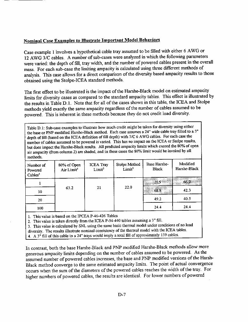
Nominal Case Examples to Illustrate Important Model Behaviors

Case example 1 involves a hypothetical cable tray assumed to be filled with either 6 AWG or

12 AWG 3/C cables. A number of sub-cases were analyzed in which the following parameters

were varied: the depth of fill, tray width, and the number of powered cables present in the overall

mass. For each sub-case the limiting ampacity is calculated using three different methods of

analysis. This case allows for a direct comparison of the diversity based ampacity results to those

obtained using the Stolpe-ICEA standard methods.

The first effect to be illustrated is the impact of the Harshe-Black model on estimated ampacity

limits for diversity cases as compared to the standard ampacity tables. This effect is illustrated by

the results in Table D. 1. Note that for all of the cases shown in this table, the ICEA and Stolpe

methods yield exactly the same ampacity regardless of the number of cables assumed to be

powered. This is inherent in these methods because they do not credit load diversity.

Table D. 1: Sub-case examples to illustrate how much credit might be taken for diversity using either

the base or PNP modified Harshe-Black method. Each case assumes a 24" wide cable tray filled to a 3" depth of fill (based on the ICEA definition of fill depth) with 3/C 6 AWG cables. For each case the

number of cables assumed to be powered is varied. This has no impact on the ICEA or Stolpe results, but does impact the Harshe-Black results. All predicted ampacity limits which exceed the 80% of open air ampacity (from column 2) are shaded, and in these cases the 80% limit would be invoked by all methods.

1. This value is based on the IPCEA P-46-426 Tables 2. This value is taken directly from the ICEA P-54-440 tables assuming a 3" fill.

3. This value is calculated by SNL using the same basic thermal model under conditions of no load

diversity. The results illustrate nominal consistency of the thermal model with the ICEA tables.

4. A 3" fill of this cable in a 24" trays would imply a total fill of approximately 139 cables.

In contrast, both the base Harshe-Black and PNP modified Harshe-Black methods allow more

generous ampacity limits depending on the number of cables assumed to be powered. As the

assumed number of powered cables increases, the base and PNP modified versions of the Harsh

Black method converge to the same estimated ampacity limits. The point of actual convergence

occurs when the sum of the diameters of the powered cables reaches the width of the tray. For

higher numbers of powered cables, the results are identical. For lower numbers of powered

D-7

Number of 80% of Open ICEA Tray Stolpe Method Base Harshe- Modified

Powered Air Limit' Limit2 Limit' Black Harshe-Black

Cables4

1 :215 66:210 .63.2 21 22.0 68. 42.3

20 49.2 40.5

100 24.4 24.4

cables, the two methods yield significantly different results, the PNP modified method being significantly more conservative.

The primary point to be taken from these results is that the credit given for diversity in either the base or PNP modified Harshe-Black methodology can be very significant. Indeed, for certain of the cases, the "global" 80% of open air ampacity limit would be the only active limit. Even given this constraint, the calculated ampacity limit for some cases was tripled in comparison to the nominal ICEA limits for a non-diverse tray (63 A based on 80% of the open air ampacity versus the nominal limit of 21 A). The question which remains unanswered by these examples is "is this realistic?". This question will be taken up further in below in the context of validation of the method.

The second feature to be illustrated is the impact of the cable tray width on the estimated ampacity limits. This is shown in Table D.2, and is especially important because of the change introduced in this behavior by the PNP modifications of the Harshe-Black method. The results show that the base Harshe-Black methodology is more prone to the prediction of absurdly high ampacity limits for cases with only a few powered cables. Note that the meaning of "few" in this context depends on the cable diameter and tray width but is generally related to cases where the sum of the diameters of the powered cables is less than the width of the tray. For these cases, the 80% of open air limit would be invoked, but even this limit may be excessive under certain of these circumstances. The base Harshe-Black methodology for these cases is clearly unrealistic, and places an undue emphasis on the role of cable tray width in the assessment of localized cable heating behavior. Based on these results, SNL cited the following finding and recommendation:

The excessive weighting of the cable tray width provided by the base Harshe-Black method represents a serious and unreasonable flaw in the base method as published by the Authors. It is recommended that the base Harshe-Black methodology should not be accepted for use in the assessment of nuclear power plant cable ampacity limits.

In contrast, the PNP implemented modification to the base methodology has a significant moderating impact on this behavior. Recall that the PNP modification limits the width of the tray section analyzed; hence, the localized heating effects are more realistically modeled. One can also note that for the cases with only a few powered cables (in this case this applies to the cases with either 1 or 10 powered cables) the modified PNP method yields the same ampacity limit regardless of tray width. This is because the "width" of the powered cables has not yet reached the width of the tray in either case, a 12" or 24" tray. Hence, the estimated ampacity limit is the same for both. This is indeed quite encouraging and offers some hope that the modified method as implemented by PNP might be acceptable.

D-8

Table D.2: Sub-case example to illustrate how cable tray width can impact the estimated cable tray

ampacity under various method of analysis. Each case assumes a cable tray filled to a 3" depth of fill

(based on the ICEA definition of fill depth) with 3/C 6 AWG cables. For each case the number of

cables assumed to be powered is varied. This has no impact on the ICEA or Stolpe results, but does

impact the Harshe-Black results. Again, the shaded entries indicate ampacity limits that exceed the "global" 80% of open air ampacity limit (from column 2).

Number of 80% of Open ICEA Tray Stolpe Method Base Harshe- Modified

Powered Air Limit4 Limit' Limit2 Black Harshe-Black

Cables3

Results with 1 Powered Cable:

12" Tray 352 .662

63.2 21 22 24" Tray 49. 4052

Results with 10 Powered Cable:

12" Tray 49.2 42.3

63.2 21 22 24" Tray 4. 44 42.3

Results with 20 Powered Cables

12" Tray 35.6 35.6 63.2 21 22

24" Tray 49.2 40.5

Results with 40 Powered Cables:

12" Tray 26.5 26.5 63.2 21 22

24" Tray 24.4 24.4

Notes:

1. This value is taken directly from ICEA P-54-440 table 3-3. 2. This value is calculated by SNL using the same basic thermal model with no diversity assumed to

illustrate nominal consistency of the model with the ICEA tables. 3. A 3" fill of this cable using the ICEA definition would imply a total of approximately 69 cables

present in the 12" tray and 139 in the 24" tray. 4. The IPCEA P-46-426 open air limit for a 6 AWG 3/C cable is 79A.

Validation of the Harshe-Black Method by the Original Authors

The original work by Harshe and Black provided only very limited comparative validation of the

base method. In particular, the original Harshe-Black paper does include one figure (see authors'

Figure 2) in which field measured cable temperatures were compared to estimated cable

temperatures obtained using the base as-published diversity method. The values are uniformly

conservative, indicating a nominally conservative model. However, there are many points that

would be of interest that are not adequately documented in the paper.

D-9

For example, how the field measurements were performed has not been adequately explained. It would appear that all of the measured cable temperatures are based on the cable surface temperature rather than conductor temperature. Ampacity limits should be based on the conductor temperature and these will be higher than the cable surface temperature. It is also unclear how the thermal model was implemented to simulate the measured trays (for example, whether the cable ampacities at the time of the testing were measured or simply assumed). It is also unclear how wide of a selection of cable trays was examined and whether or not the selection is sufficient to validate all applications (a single table citing a range of certain tray parameters is provided). Finally, the authors cite that some of the data was not presented because it is considered suspect. If this data indicated some cases of non-conservative performance, then explicit explanations of the presumed discrepancies and a review of the authors conclusions of non-applicability would be appropriate.

The validation results presented in the original paper show no cases where the results are nonconservative. As noted in SNLs own example cases there are cases where the base method aspublished would clearly be inappropriate. A full validation study would be expected to explore these cases as well. Given that the method can yield unreasonable results, it is appropriate to limit the application of the method to ensure that such results are not credited. A complete validation study would verify that the model can accurately or conservatively predict operating temperatures given the actual conditions at the time of the measurements. Given the results of the SNL case studies, as discussed above, SNL concluded that the model validation was inadequate. Of particular concern is the obviously questionable treatment of tray width effects.

The Stolpe Diversity Test

There are only a limited selection of tests currently available upon which this type of validation might be reasonably based. One is Stolpe's diverse cable tray test as reported in his original paper

(see Ref 13 in the Section 8.1 of this report). A second is a series of six diversity tests performed by TVA for the Browns Ferry plant. These TVA tests will taken up below.

As a part of his original work, Stolpe ran one test involving a diverse load cable tray. The tested tray included nine different types and sizes of cables. In his first test all of the cables in the tray were powered to an equal level of heat intensity, that value that his model predicted would result in a 50'C hot-spot temperature rise (90'C cable temperature). In a second test of this same tray

only three of the nine cable groups were powered, and each was powered to the same ampacity as in the first test. Hence, for both cases, the heat intensity of the powered cables is constant. This makes the analysis much simpler.

Note that there does appear to be a discrepancy regarding the actual ampacity of the 6 AWG cable in these two tests. In particular, Stolpe's Table II indicates that the predicted ampacity limit for the 6AWG cable in a 20% fill should be 51 A. This is the ampacity to which these cables should have been subjected in these tests. However, the data plot indicates that the actual test ampacity for this cable was significantly less than 50 A (approximately 37A based on the plot).

D-10

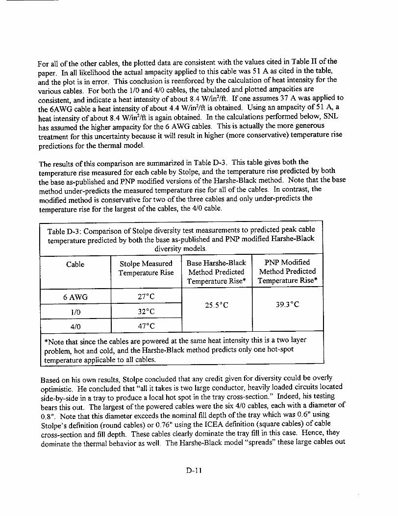
For all of the other cables, the plotted data are consistent with the values cited in Table II of the

paper. In all likelihood the actual ampacity applied to this cable was 51 A as cited in the table, and the plot is in error. This conclusion is reenforced by the calculation of heat intensity for the

various cables. For both the 1/0 and 4/0 cables, the tabulated and plotted ampacities are

consistent, and indicate a heat intensity of about 8.4 W/in2/ft. If one assumes 37 A was applied to

the 6AWG cable a heat intensity of about 4.4 W/in2/ft is obtained. Using an ampacity of 51 A, a

heat intensity of about 8.4 W/in2/ft is again obtained. In the calculations performed below, SNL

has assumed the higher ampacity for the 6 AWG cables. This is actually the more generous

treatment for this uncertainty because it will result in higher (more conservative) temperature rise

predictions for the thermal model.

The results of this comparison are summarized in Table D-3. This table gives both the

temperature rise measured for each cable by Stolpe, and the temperature rise predicted by both

the base as-published and PNP modified versions of the Harshe-Black method. Note that the base

method under-predicts the measured temperature rise for all of the cables. In contrast, the

modified method is conservative for two of the three cables and only under-predicts the

temperature rise for the largest of the cables, the 4/0 cable.

Table D-3: Comparison of Stolpe diversity test measurements to predicted peak cable

temperature predicted by both the base as-published and PNP modified Harshe-Black diversity models.

Based on his own results, Stolpe concluded that any credit given for diversity could be overly

optimistic. He concluded that "all it takes is two large conductor, heavily loaded circuits located

side-by-side in a tray to produce a local hot spot in the tray cross-section." Indeed, his testing

bears this out. The largest of the powered cables were the six 4/0 cables, each with a diameter of

0.8". Note that this diameter exceeds the nominal fill depth of the tray which was 0.6" using

Stolpe's definition (round cables) or 0.76" using the ICEA definition (square cables) of cable

cross-section and fill depth. These cables clearly dominate the tray fill in this case. Hence, they

dominate the thermal behavior as well. The Harshe-Black model "spreads" these large cables out

D-11

Cable Stolpe Measured Base Harshe-Black PNP Modified Temperature Rise Method Predicted Method Predicted

Temperature Rise* Temperature Rise*

6 AWG 270 C 25.5 0C 39.3 0 C

1/0 32°C

4/0 470 C

*Note that since the cables are powered at the same heat intensity this is a two layer

problem, hot and cold, and the Harshe-Black method predicts only one hot-spot temperature applicable to all cables.

into a relatively thin layer; 0.33" for the as-published model and 0.58" using the PNP modified model (both values based on the ICEA definitions of fill depth).

The TVA Browns Ferry Diversity Tests

During 1988/89 the USNRC was engaged in the review of certain ampacity studies submitted by Tennessee Valley Authority (TVA) for the Browns Ferry Nuclear Plant.' During the course of

that review the licensee provided a test report documenting the results of a study performed to

validate TVA's own methods used to credit load diversity in ampacity assessments. The tests are

quite unique and are readily applicable to a validation of the Harshe-Black method.

In brief, TVA assembled a single cable tray 18" wide and 4" tall that was filled to an overall fill

depth of 2.16" (ICEA definition) using 120 lengths of a single-conductor #1/0 light power cable. The tray was first run to establish a nominal baseline ampacity limit with all cables powered as would normally be done today, for example, in an IEEE-848 ampacity tests. The 120 conductors

were then re-connected into four separate cable groups of 30 cables each using a random selection of conductors to form each group. These groups were then powered independently to predetermined diverse ampacity values, and the resulting cable temperatures measured in a selection of locations.

Figure D-1 provides a simple schematic to illustrate the location of the cables in each of the four

diversity groups. It is especially important to note that the groupings do include some significant clustering of the powered cable groups. For example note that at the left side of the tray, as seen

in the figure, there is a cluster of group 1 and group 4 cables that is 4 cables wide by 4 cables high. Also, near the center of the tray there is a second clustering of group 1 and 4 cables. As

discussed further below, in all of the tests both the group 1 and group 4 cables were powered

during testing. This factor is important in interpreting the results as will be discussed below.

1 1X X X (X j 2 4 4 2 21 1 2 2, A 2 1 14 4 2 2 1 1 2 2

Figure D-1: Schematic representation of the TVA diversity test cable tray indicating the four cable power groups. Note that groups 1 and 4 were powered to some level in all tests.

1The original licensee submittal under review by the USNRC was documented under TVA

cover to the USNRC Document Control Desk dated July 7, 1988. The review was coordinated by Mr. Hukam Garg, USNRC/NRR, and was supported by SNL under the terms of a general

technical services contract for licensee and vendor Equipment Qualification inspections. This

discussion is based on SNL records of this effort.

D-12

There are some inherent limitations to this data. The most significant is that there was no

systematic attempt to locate the actual hot spots in the tray. This is because not all of the cables

in the tray were instrumented. Rather, a large number of preselected cables were instrumented

prior to installation, many of these cables concentrated around the center of the tray with a more

limited selection of thermocouples at the edges of the tray. The cable groupings were then chosen

at random after installation. Hence, the actual hot spot temperatures may not have been truly

captured. This is somewhat mitigated by the fact that several of the group 1 and 4 cables are

present in a cluster near the center of the tray, and many of these cables were, in fact, instrumented. Hence, it can be concluded that the measured temperatures did characterize at least

one of the two highest power density regions in the tray. However, the data should be viewed as

somewhat suspect with the actual hot-spots somewhat uncertain. Nonetheless some indication of

the model behavior for these cases can be discerned.

A total of five diversity tests were performed. In each test at least one, and typically two, of the

cable groups were not powered at all. The other cable groups were powered using from 60% to

150% of the nominal baseline ampacity measured during the original test with all cables powered.

Table D-4 summarizes the conditions in each test.

All conductor loads are expressed as a percentage of the baseline ampacity measured in

the original non-diverse load test of the same cable tray.

The reported test data includes the measured maximum cable temperature in each test. Given this

data it is quite simple to simulate each test using the Harshe-Black methodology. In this case, the

cables in each group represent one full layer of cables across the width of the tray. Hence, there

will be no distinction between the base as-published method and the PNP modified method. Either would yield identical results.

To perform the validations, SNL implemented a simple version of the Harshe-Black method

designed to estimate the maximum cable temperature rise given the set ampacity loads for each

D-13

Table D-4: Summary of TVA diversity test power loads

Conductor Loading Test No. TestNo._ Group 1 Group 2 Group 3 Group 4

211 120% 0% 100% 80%

212 120% 0% 0% 80%

213 130% 0% 0% 90%

214 110% 0% 0% 60%

215 150% 0% 0% 80%

group of cables. This required some relatively modest modification to the model execution, but maintained all features and assumptions of the base model.

In the modeling, the choice of cable groupings was quite obvious. The cables were simply

separated into three groups as follows: the hot cables were those with the highest loading (group 1), the cold cables were those with no load (group 2 for test 211 and both groups 2 and 3 for the other tests), and the warm cables were the remaining cables (groups 3 and 4 for test 211 and group 4 for the other tests). Note that for the warm group in test 211 there are two different ampacity loads applied in the test. Consistent with the Harshe-Black approach, the simulation used the actual heating load based on a summation of the individual cables. Also note that all electrical resistance values are taken as those at 900C.

The results of this exercise are illustrated in Table D-5. Note that in each case the Harshe-Black method has conservatively estimated the maximum cable temperature as reported by TVA. That is, the predicted temperature rise is uniformly greater than the worst-case temperature rise reported in the tests. This is quite encouraging and provides a powerful basis for acceptance of the method under these conditions. One factor that is not accounted for by these tests is the mixing of very large heavily loaded cables with smaller power cables, the problem posed by the Stolpe test results.

Table D-5: Summary of Harshe-Black method simulation results for the TVA diversity tests.

Test No. Measured Peak Cable Calculated Peak Cable Temperature Rise (C) Temperature Rise (C)

211 35.38 47.1

212 27.38 35.1

213 32.19 41.6

214 20.58 27.3

215 39.13 48.3

Review Findings and Recommended Application Restrictions

In its original review SNL found that both the base Harshe-Black method (as originally published

by the authors) and the modified PNP version of the method (in which the width of the analyzed

section may be limited) can result in very significant increases in cable ampacity limits as compared to the ICEA/Stolpe methods that do not credit diversity. Some of the example cases

explored by SNL resulted in tripling of the estimated ampacity limit. Clearly, load diversity can

significantly impact cable operating temperatures under realistic installations conditions. Whether

D-14

or not the diversity credit allowed by this method is entirely warranted under all circumstances has

not been demonstrated either by the authors, by PNP, nor by the SNL studies documented here.

The remaining hurdle is that only limited and sparsely documented validation of the base methodology is available, and this validation has clearly not adequately explored the potential

application limitations. Supplemental validation studies performed by SNL did reveal at least one

potential weakness of the method. That is, when the cable load included very large power cables

that are heavily loaded the method may underestimate cable temperature rises. This is an artifact

of the way in which the heavily loaded cables are modeled as a relatively thin layer across the

width of the section analyzed by the thermal model. This may not adequately treat the localized

heating effects associated with power cables that are large in comparison to either the overall tray fill depth, or to other heavily loaded cables that are physically smaller.

Given this, the ultimate application limits of the methodology remain uncertain. The above

discussions have identified some of the potential limitations, and in fact, the modifications implemented by PNP in its own applications directly address one of the most serious of these

limitations. The most significant potential limitations are:

The base (as published) method may over-state the role of heat dissipation across the width of the tray when there are only a very few powered cables present. The PNP modifications adequately address this point of concern.

Ampacity limits for large cables may be overstated. To some extent this is also an inherent

limitation of the Stolpe/ICEA methods. Imposition of a global limit of 80% of the open

air ampacity provides one check on this possibility; hence, adequate recognition and proper application of this constraint in practice is necessary.

If some subset of the powered cables are located in close proximity to one or more large heavily loaded cables, then ampacity limits may be overstated. The PNP modification to the method reduces the potential magnitude of the error, but does not entirely eliminate it.

It is this problem that was the primary basis for Stolpe's recommendation that diversity not be credited in cable tray ampacity assessments.

Overall it was concluded that some constraints on the application of the method are needed to

prevent this potential from being realized, and this is taken up further below. Based on these findings, SNL made the following recommendations regarding the acceptability of the base method as originally published by Harshe-Black:

The base Harshe-Black methodology as originally published by the authors is deficient for

two main reasons: (1) it may allow an overly optimistic treatment of potential localized heating effects under certain circumstances and (2) it will over-state the role of heat

dissipation within the cable mass for cases involving a small number of powered cables.

D-15

Hence, it is recommended that this version of the methodology should not be accepted for

use in the assessment of nuclear power plant cable ampacity limits.

With regard to the modified Harshe-Black method used in the PNP assessments:

PNP implemented critical modifications that directly addresses the most serious shortcoming of the base Harshe-Black method (involving limitations placed on the width of the analyzed tray section). Validation cases examined by SNL indicate a nominal ability of the method to conservatively predict cable operating temperatures for a range of conditions involving diverse cable loads. It can be anticipated that for most situations, the PNP modified method will result in reasonable-to-conservative estimates of the actual ampacity limits, or alternately cable operating temperatures, for diverse load cable trays.

However, the validation also demonstrated that the method cannot adequately address cases that include relatively large, heavily loaded power cables.

It was recommended that additional constraints be placed on the application of the Harshe-Black method as modified by PNP to ensure that inadvertent cable overloads do not occur. The USNRC's acceptance of the PNP applications was predicated on an assumption that these restrictions would be implemented. (They were, in fact, implemented by PNP as documented in

the final licensee submittal on the subject.) Specifically, it was recommended that the modified

PNP version of the Harshe-Black method be accepted for use subject to the following restrictions:

The method should not be applied to any tray that includes two or more cables that are (1) powered to at least 80% of the nominal ICEA cable tray ampacity limit, and (2) whose diameter exceeds the tray fill depth when calculated using the ICEA definitions.

In formulating the thermal model, a lower bound should be established on the

combined thickness of the central high-intensity or "hot" and "warm" cable layers to prevent excessive "thinning" of this layer and to more accurately reflect the presence of larger cables in this group. These two groups will likely represent the

total heating source for the thermal model. SNL recommends that this lower bound should be no less than 80% of the diameter of the largest cable in the hot and warm groups.

The first restriction is specifically intended to address the Stolpe test results and the concerns

expressed in his pioneering work on cable tray ampacity. It would disallow use of the diversity

method in cases where the potential for a smaller cable to be "sandwiched" between two larger

heavily loaded power cables does exist. The second restriction is intended to address the potential

clustering of a number of smaller cables in close proximity to a larger powered cable. By placing

a lower bound on the combined thickness of the "hot" and warm cable layers, potential clustering

effects will be more reasonably accounted for. This approach will ensure that the heating zone is

modeled with a thickness that is at least nominally consistent with that of the larger cables.

D-16

SNL did acknowledge in its original review that these recommended restrictions are somewhat arbitrary. They are intended to address demonstrated limitations and shortcomings of the thermal

model, but the cited numerical constraints are not well based in scientific evidence. There is

simply not enough data available to fully assess the limitations of the method. At the same time, SNL also found that the level of model validation was not sufficient to warrant the unlimited applicability of the method. Indeed, SNL's own validation efforts did illustrate that the model can

underestimate cable operating temperatures under certain conditions, especially involving very

large power cables. Hence, these restrictions are recommended pending the availability of more

complete validation data sufficient to address the cited shortcomings of the model.

Summary of Findings and Recommendations

Based on the USNRC review of the model it was recommended that the base Harshe-Black method as originally published should not be accepted for use in nuclear plant ampacity assessments. However, it was also recommended that the modified Harshe-Black methodology as

implemented by PNP and subject to two restrictions as cited above should be accepted by the USNRC.

The recommended restrictions are intended to ensure that unreasonable ampacity limits are not

obtained for cases involving a mixture or very large and smaller power cables. Including the

recommended application restrictions, there is reasonable assurance that the PNP modified method can be used to demonstrate that actual cables are operating at or below their rated temperature limits.

MATHCAD Implementation of the Harsh-Black Diversity Model for Random Fill Cable Trays

SNL has implemented a somewhat simplified version of the Harshe-Black model of diversity credit for random fill trays as described in the attached MATHCAD workbook file. This file includes both the base as-published methodology and the PNP modified methodology in which the width of the section is limited in cases of few powered cables.

SNL's implementation is relatively simple and includes some simplifications and idealizations that make it unsuitable for actual applications. The implementation is intended only to serve as a "sounding board" to explore the impact of the model on ampacity limits. The SNL simplifications are:

External convection is treated using the same heat transfer coefficient for both the top and bottom surfaces of the tray. This treatment is specifically intended to ensure consistency with Stolpe's thermal model.

There is no adjustment of cable electrical resistance for temperature. All values are taken

as the resistance at 90'C. This is generally fine in the hot zone and as long as the hot-spot

D-17

is 90°C, but will be conservative when estimating heat loads for the warm and cold zones, and for cases where the hot spot does not reach 90'C.

The version documented in this appendix is actually a two zone version (hot and cold). Incorporation of a third warm zone is relatively straight-forward. Indeed, certain of the validation results discussed in Appendix B did include some three zone cases.

SNL has only exercised the model for cases where all of the cables in a given layer are powered to the same heat intensity. No adjustments to the temperature rise for individual cables are made.

The initial calculation assesses the temperature rise within the cable mass as per the simplified one-dimensional heat transfer model. This establishes the surface temperature of the cable mass. The second part of the model then calculates the rate of heat transfer away from the cable mass to

the ambient by convection and radiation using the estimated cable surface temperature and the specified ambient as the driving thermal potential.

The limiting ampacity is derived by setting up a single solve block that automatically matches the specific temperatures, and the various heat flow rates in the thermal model. The model can also predict Stolpe/ICEA limits by simply matching the external heat transfer to the full non-diversity based cable heat load.

D-18

An implementation of the Harshe Black Diversity-Based ampacity assessment method for cable

trays. This version includes both the base methodology (as per the paper) and the method as

modified by Palisades for actual applications. It also includes a nominal Stolpe/ICEA calculation

at the end for reference purposes.

Programmed by: S. P. Nowlen, Sandia National Laboratories, November-December 1997

The base (stored) case involves the analysis of a given number or powered cables in a tray with a

set fill depth. It is assumed that all other cables are not powered at all, so there are only two

regions, the high intensity band and the low-intensity or unpowered bands.

Note that in this version, the ICEA definition of "square cables" is used throughout for both cross-section and for depth of fill assumptions.

Imprortant Note: "Mathcad 'trick': If you are using a version older than the 4.0 PC version, then

you need to equate temperature to charge units since there was no fundamental temperature unit

provided in these older versions of the program. Hence, you must insert a formula line that sets:

K- 1 * coul (This is not a real equation in this implementation, only a text block)

Then use K as fundamental unit. For newer versions, this in not necessary because K (and R) is

already defined as a fundamental unit. You do still need C to K and F to R conversions if you want

to work in C or F. We are using 4.0, but will occassionally want temps in C so:

CtoK := 273.16-K

Set up initial parameters:

The Cables: In this case, we assume a fill of 31C 6 AWG cables using the diameter given in ICEA P 54-440 Table 3-3:

d cable:= 0.72-in R cable:= 5.15-10 p cable :400-K

ft watt

n conductors:= 3 6 cable:= 0.9

The thermal conditions to meet:

T hot:= 90-K + CtoK Tamb:= (40-K + CtoK)

The Tray:

w tray:= 12-in d fill:= 3-in

Set some Physical Constants:

s steel:= 0.7 steel emissivity (not used in this example)

a := 0.530-10 8 - watt Stephan-Boltzmann

Define The Power/diversity Loading:

If you want to simulate the Stolpe Answer, one way is to simply set all cables possible given

the dfill above as powered (that is, no diversity at all). Recall that we use the ICEA definition of fill depth in this analysis so to do this use the following equation:

w tray-d fill n powered -d 2 n powered = 69.444

d cable

D-19

While this is a rather arbitrary and probably non-integer number, it will be internally self consistent As an alternative, one can simply specify the number of powered cables as follows:

n powered:= 10

Recall that the last set value will be used below, so to use full fill, must delete the equati immediately above. This example continues with 10 powered cables.

Now we can calculate the dimensions of the high-intensity band for each method:

The base method:

W base := w tray

n powered cable2 hbase "

w base

The modified method:

W mod := n powered'd cable +0.5 -d fill

w base = 12-in

h base = 0.432 -in

W mod = 8.7 -in

Cannot exceed tray width so do an upper bound check and reset if exceeded:

W mod:= if(w mod>W trayW trayW mod) W mod = 8.7 -in

Now get the corresponding band hieght for the modified method:

n powered-d cable h mod:=

w mod h mod = 0.596-in

The solution will use a solve block so we first set up our callable functions for which we will late seek self-consistent solutions.

Cable Heating Rate:

2 Q cable(, cable"') := I cable *R cable-n conductors'n

Cable Zone Heat Intesity (NOT USED IN THIS EXAMPLE):

Q cable(, cable,n powered) HI(I cable,A zone) :A zone

Cable mass Temperature Rise (recall we have just one heat zone at center):

dT mass(Q, h hot, W mass) := QP cableht (d fill- h hot) 4 -w mass [ 2

Convection coefficient:

watt 4T

h surT sur := 0.101----- ( surf- Tamb)

D-20

Set up the overall external heat transfer expressions:

Q conv(T surfA suhf-):h T su-A surf (T surf- T amb)

Q rad(T surfA surf, surf surfA surf(T surf - Tamb)

Q external(T surfA surf,' surý : Q conv(T surfA surý +~ Q rad(T surfA surf, surý

That is the "physics", now we just need a solution for our case. To do this we set up a solve blo to get a simultaneous solution to a multiple equation set that will match temperatures and heat fluxes so that the full thermal model is self-consistent This is a very simple case with two equations and two unknowns. In this implementation we need to match the external heat trans to the internal generation rate, and find the surface temperature that provides this match.

For the base method:

First need to "seed" the answer

I base:= 10-amp

T surO= 50-K + CtoK

Now we set up our solve block:

Given

Q extema(T surf 2 w basee cable) =Q cable(I basen powered)

T sur&T hot- dT mass(Q cable(1 base, n powered), h base, W base)

IIbasel T surfJ Find (1 base,T su

And the base method answer is:

I base =49.182-amp

T surf- CtoK =61.554-K

For the modified method: Seed the solution:

I mod:= 10-amp

T surf:= 5 0 -K + CtoK

Set up the Solve block

Given

Q extema(T surf,2 "w mod,' cable)=Q cable(I mod,n powered)

T surf=T hot- dT mass(Q cable(, mod'n powered), h mod, W mod)

I umod]

T surfJ. Find (I mod, T sur

D-21

And the Modified case answer is:

I mod = 42.252,amp

T surf- CtoK = 61.894,K

As a final step, we solve the same case using the nominal Stolpe/ICEA Method. Recall that in this case there is no credit for diversity.

First we calculate the number of cables making up a full fill of the specified cable and specified depth of fill for the specified cable tray width (using the ICEA definition)

w trayd fill

nbStolpe : a 2 n Stolpe = 69.444

Now we do our solution: Seed the answer:

I Stolpe:= 10-amp

T surf:= 50-K + CtoK

Set up the Solve block:

Given

Q external(T surf 2 w trayc cable) =Q cable(I Stolpe'n Stolpe)

T surf T hot- dT mass(Q cable(, Stolpen Stolpe) ,d fil, W tray)

IStolpe] Find(t StolpeTsur•

T surf (

And the "Stolpe" answer is:

I Stolpe = 22.005 -amp

T surf- CtoK = 68.694.K

Let us recap our different solutions:

Recall the Case:

W tray= 12-in d fill= 3 .in n powered = 1 0

Recall the solutions:

I base = 49.182.amp The Basic Harshe-Black Solution

I mod =42.252,amp The Modified Harshe-Black Solution

I Stol p = 22.005 -amp The Nominal Stolpe/ICEA Solution

D-22

Appendix E

The Leake Cable Tray Diversity Model

Overview

The USNPRC review of the Leake model (Ref. E-1) was conducted in conjunction with a licensee submittal from Palo Verde Nuclear Generating Station. The specific intent of the Leake model is to allow some credit for diversity in cable power loads as a part of the ampacity assessment process. As the original paper cites, the widely accepted ICEA P-54-440 method, which derives from the work of Stolpe, assumes no diversity in its cable ampacity assessments. This is, recognizably, a conservative approach to analysis. The objective of the Leake method is to relax this conservatism and to allow for at least some diversity credit.

One important factor to note is that the Leake method is only applied to open cable trays. The method is intended to address the baseline ampacity limits of the cables. The licensee in this case intended to then apply the appropriate ampacity derating factor (ADF) to the baseline ampacity estimates to determine the derated ampacity limit for a clad cable tray. This approach was accepted by the USNRC.

The General Approach

Leake draws an excellent comparison between the various proposed methods of analysis in which some credit for diversity is taken, including the "Watts per foot" method. A significant

portion of the paper is devoted to comparisons between the various approaches, and a demonstration that the model proposed by Leake is more conservative than those that have been put forth in the past.

The general approach taken by Leake is based on a single modification of the Stolpe assumptions. In particular, Leake maintains Stolpe's (Ref. E-2) model of heat transfer within a cable mass and the concept of uniform heat intensity within the tray. However, Leake modifies the treatment of cable mass-to-ambient heat transfer by using a reduced heat load based on actual cable loadings for this step of the analysis. That is, for in-tray heat transfer behavior a conservative non-diversity based heat load is assumed. For tray-to-ambient behavior, the lower actual heat load of the cables including diversity is used.

To elaborate, in Stolpe's model all the cables in a tray are assumed to be loaded to an equal level based on the rate of heat generation per foot of tray and per unit of cable cross-section, the "heat intensity." This method assumes no diversity. For the in-tray behavior, that is conduction within the cable mass, a simplified expression for heat transfer in a one-dimensional mass with uniform heat generation is used to estimate the temperature rise from the surface of the mass to the hot spot at the center of the tray. In Stolpe's model this same overall heat load is then used to estimate the temperature rise between the ambient and the cable surface (the tray-to-ambient heat

E-1

transfer) based on simple convection and radiation correlations. The result is an estimate of the overall ambient to cable hot spot temperature rise. The heat load, or heat intensity, is adjusted until the predicted cable hot-spot temperature matches the maximum allowable temperature rating of the cables. The critical point to observe is that the exact same conservative heat load is used for both the in-tray and tray-to-ambient thermal behavior.

Leake's model makes the exact same assumptions for the in-tray behavior with no credit given to diversity in this step of the analysis. However, when the heat transfer between the cable mass and the ambient is considered, the tray-to-ambient behavior, Leake's method credits diversity by using the lower actual heat load of the cables in the tray rather than the conservative estimate based on worst-case uniform heat generation. The actual heat load on a tray may be just a small fraction of the heat load assumed in the Stolpe calculations. Using this method, the role of trayto-ambient heat transfer in the overall process will be significantly reduced. For many cases, the in-tray behavior will dominate the calculation.

The net effect of this practice is a compromise solution that ranges between the method of Stolpe and that of other diversity based methods including the "Watts per foot" method. Leake acknowledges that the previously proposed diversity crediting methods including those outlined by Harshe and Black (Ref. E-3) can lead to non-conservative results, especially in the case of a highly diverse cable tray (a tray with only a few energized conductors). It is Leake's contention that by retaining Stolpe's cable mass thermal model, the method does assess the ampacity load for individual cables.

The Critical Parameters and Leake's Model

As is obvious from the discussion above, there are two primary heat transfer behaviors of interest in a cable tray ampacity assessment; namely, in-tray behavior and tray-to-ambient behavior.

The in-tray behavior as modeled by both Stolpe and Leake is strictly a conduction problem. In reality, most trays will experience some convective air currents passing through the tray, but this effect is not modeled in any way (this is one source of conservatism in the in-tray treatment). As a conduction problem, the only parameters with a direct impact on the analysis results are the thickness of the cable mass (the tray depth of fill) and the assumed thermal conductivity of the cable mass. Given the assumptions of the Stolpe model, there are no other "floating" parameters. Virtually all such analyses, including Leake, cite the Stolpe assumed value for the cable mass thermal conductivity (See Appendix A for a discussion of cable thermal conductivity.) It is important to note that the assumed width of the tray has no impact on the results of the in-tray analysis.

In contrast, the tray-to-ambient problem is a strictly convection/radiation problem. As such it is dominated by the assumptions regarding the surface of the cable mass. These include in particular the emissivity of the surface, and the convective heat transfer coefficient. A third critical parameter in general is the surface area assumed in the analysis. In the specific case of

E-2

Stolpe's model, the assumed width of the tray has only a very minor impact on the analysis. (Tray width does play a very minor role through the convection coefficient if the full expression

is used. See ICEA P-54-440 and Appendix B of this report for a discussion of the impact of

width on calculated ampacity limits.) Using Stolpe's method one will obtain virtually the exact

same ampacity result for a 6" tray as one will for a 48" tray with the same depth of fill.

Leake's treatment of the tray-to-ambient behavior introduces one significant change to the this process. That is, in Leake's model, the heat load for the tray-to-ambient analysis is fixed based on the actual cable loads. However, this heat transfer is assumed to occur across the entire surface of the cable mass. Hence, as the tray width increases, the convective and radiative heat transfer rates also increase. Given this, the method will predict different ampacity limits for the same cable based only on changes in the tray width. This is an obvious potential criticism of the Leake

method that will be explored in greater detail below. In particular, unrealistic results might be expected for wide trays with only a very few powered cables and limited fill depth.

It should also be noted that Leake acknowledges this limitation. In particular, the Leake paper includes the following statements:

"In cases where the depth of fill is close to the diameter of the largest cables, all of the methods which credit diversity may be non-conservative, and (the Stolpe method) is more appropriate. For example, in a tray containing a single layer of cables, the heat dissipated by a few current-carrying cables located side-by-side would not spread evenly to all of the unenergized cables, some of which could be a significant horizontal distance away. Hot spots could occur where the energized cables touch each other, and may not be identified by (the diversity crediting methods). This is illustrated in (certain of Stolpe's test results). In a tray with a 0.76" calculated depth of fill, the temperature of an energized #4/0 cable, with a diameter 105% of the calculated depth of fill, dropped only 1 'C when a number of the other cables were deenergized."

Regarding Leake's citation to the Stolpe tests, it should be noted that Stolpe and ICEA P-54-440 use somewhat different methods to calculate depth of fill (round versus square cables respectively as discussed in the body of this report). If the ICEA method (square cables) is used, then the specific #4/0 cable cited in this passage would have a diameter equal to about 82% of the calculated fill depth. PVNGS does use the ICEA definitions for fill depth and cable crosssection; hence, in this case basing the insight on comparison of cable diameter to the ICEA fill depth is more appropriate.

Exercising the Model

SNL explored, to a limited extent, the results of the Leake method including a modest exploration of certain sensitivities in the model input parameters. For illustrative purposes, SNL

chose to model a number of cases involving one or more powered 3-conductor, 12 AWG cables. The physical diameter of the cable was assumed to be 0.43" which is consistent with the ICEA

E-3

assumptions as set forth in Table 3-3 of P-54-440. For all cases, a 40TC ambient and a 90'C conductor temperature were assumed. This allows a direct comparison of the modeling results to the ICEA ampacity limits.

The implemented MATHCAD model is presented below. In implementing the model, SNL first verified that it could reproduce the ICEA limits directly. This verified the basic implementation of the heat transfer correlations to be consistent with Stolpe and the ICEA. We then considered the alternate treatment of Leake. To exercise the model, SNL considered three fill depths (0.5, 1.0 and 3.0 inches) and three different levels of diversity, one powered cable, 10 powered cables, or 20 powered cables. SNL also considered the impact of tray width on the Leake results. The results of this exercise are illustrated in Table E. 1.

Table E. 1: summary of example calculations performed by SNL using the Leake diversity-based ampacity method.

There are several points to be observed regarding these results. One feature somewhat unique to Leake (although also applicable to the Harshe/Black layering method) is that the method can potentially overstate the importance of tray width in determining local heating effects as was discussed above. That is, Leake assumes that heat transfer occurs with equal effectiveness over the entire top and bottom surface of the cable mass, and that the surface of the mass is at a uniform temperature. By this treatment, the actual heat generated in the tray is "stretched" or "spread" over the full width of the tray and potentially "diluted" beyond the point where the thermal model reflects the real tray. Several observations in this specific regard can be made from these examples:

The impact of the tray width on the estimated ampacity was modest for most of these cases. This is because the estimated temperature rise within the cable mass generally

E-4

Fill Tray IEEE 835 Stolpe / Leake limit for Leake limit for Leake limit for Depth width open air ICEA 1 powered 10 powered 20 powered

(in) (in) limit* P-54-440 cable cables cables limit

0.5 12 19 52.1 30.7 23.5

24 55.5 38.2 30.6

1.0 12 36 13 28.8 22.5 19.1

24 29.4 25.3 22.6

3.0 12 6 10.0 9.5 9.1

24 10.0 9.8 9.6

* Open air ampacity for a 12 AWG triplex cable, 80% of open air limit cited in

brackets

dominated the ampacity assessment, and the surface heat transfer played only a limited role.

It is apparent that as the level of diversity decreased (that is as more cables were assumed to be powered) the role of the surface heat transfer increased. This is as expected since all cases for a given fill depth assume the same in-tray behavior, but the external heat load increases in direct proportion to the number of powered cables. The increasing external heat load implies a much more significant role for the surface heat transfer behavior. As was discussed above, the surface behavior in Leake's model will be influenced in direct proportion to tray width.

It is also apparent that the role of the surface heat transfer increases in importance as the depth of fill decreases. Again, this is consistent with expectations in that the role of the in-tray temperature rise decreases as does the fill depth; hence, the relative importance of the external surface behavior increases. It is likely that the importance of surface behavior is significantly overstated for the low-fill cases with high diversity (e.g., the single powered cable case).

Another point to be observed is the potential for this method to yield clearly unreasonable results:

Many of the ampacity estimates generated by the Leake model, especially including those for the lower fill depth, exceed the open air ampacity limits for a triplex configuration 12 AWG cable as taken from the IEEE 835-1994 standard. (The IEEE triplex ampacity limit is roughly equal to the NEC 3-conductor limit; 36 A versus 35 A.)

This is not surprising. In fact, the Stolpe/ICEA heat intensity method also suffers from a similar problem whenever the depth of fill in the tray is less than the diameter of the cable under analysis. Stolpe had recommended that for a given cable, the ampacity not exceed that calculated for a fill depth equal to one cable diameter regardless of the actual fill (if less than one diameter). In the ICEA P-54-440 method, a limit of 80% of the open air ampacity is established which effectively accomplishes the same goal. Clearly, some similar check on the Leake would be appropriate to ensure that unrealistic ampacity estimates are not generated or assumed.

One case that is of particular interest is the case for 20 powered cables in a 12" tray with a 0.5" fill depth (the upper right comer entry). Note that given a cable diameter of 0.43", it would require about 32 cables to reach a fill depth of 0.5". Hence, this case assumes that about 2/3 of the cables in the tray are energized. The ICEA limit for this case was 19 A whereas the Leake method would allow a 23.5 A load for each of these cables. This represents an increase of 23.7% in the ampacity limit due to crediting 2/3 diversity. This is, indeed, a significant allowance for this case. In particular, with 2/3 of the cables energized, there is a significant possibility that many of the energized cables will be located next to, or in close proximity to, each other. Hence, the allowance for the diversity may be overly optimistic.

E-5

Validation

One critical aspect of any thermal model is validation through comparison to data. Leake cites his validation basis as being primarily by implication. That is, he compares his results to the other diversity crediting methods and cites that his method is more conservative. He cites in particular that the Harshe/Black method was validated by comparison to in-plant cable performance data; hence, by implication his own "more conservative" approach is also validated by those data. However, no direct comparisons of any specific measured data to modeling assessments has been provided either in the paper or in the licensee submittal. This is not an adequate validation basis upon which to base acceptance of general and unlimited use of the approach in nuclear power plant applications.

The range of data available for this type of validation is rather limited. Stolpe, for example, included only one diversity experiment in his test set. The measurements made by Harshe/Black on actual cable at the Palisades Plant have only been presented in a very limited context, and to SNL's knowledge, no direct one-to-one correspondence between individual installation features and measured temperature data has yet been published. Most of the other laboratory tests performed to date have not involved load diversity. Hence, any validation is problematic.

In this regard, it is especially interesting to note the Stolpe test result as discussed in Section 3.5 of the main body and in Appendix D of this report. For one cable, the diverse load test resulted in a 15 'C drop in the measured cable temperature, while for another cable in the same test, the drop was only 1 °C. For the third intermediate cable, the #1/0 AWG cable, the difference in measured temperature appeared to be about 9°C. Clearly the diversity benefit to be gained is very case specific, and will depend on a number of factors.

Recommended Application Limitations

In general the Leake method represents a reasonable compromise solution that can quantify some modest relaxation of the conservative assumptions of the Stolpe/ICEA methods by allowing credit for cable- load diversity. However, the author has failed to establish an adequate basis for deciding when the method is appropriate, nor have sufficient checks been established to ensure that unrealistic results are not credited. It was recommended that a clear-cut set of limitations be established to resolve these potential concerns and the USNRC acceptance of the method was predicated on implementation of these restrictions.

The first point of concern is to ensure that clearly unrealistic ampacity limits are not credited. The recommended constraint to address this concern is essentially identical to that already provide in the ICEA P-54-440 standard:

In the application of the Leake method to diverse random fill cable trays, the maximum baseline ampacity limit, or the maximum baseline heat intensity, should under no circumstances be assumed to exceed 80% of the corresponding open air limits. That is,

E-6

any calculation that estimates a baseline ampacity limit (or equivalently the corresponding heat intensity level) that exceeds 80% of the cable's open air ampacity should be discounted and disregarded.

In addition, one important limitation to the Leake methodology was identified in the USNRC review; namely, the potential that the role of tray width might be overstated under certain circumstances where in reality a cable hot-spot might not be dissipated. Hence, SNL recommended that some specific limitations be established to prevent mis-application of the method. In order to address this specific concern the following limitation on the method should be employed:

The Leake method for crediting diversity should not be applied to the analysis of any cable whose diameter is greater than or equal to V2 the tray fill depth as calculated using the ICEA definitions of cable cross-section and fill depth.

Note that SNL has made this recommendation specific to the analysis of a given cable. That is, the mere presence of a large cable in a tray should not be an automatic basis for disallowing the method. The concern is that comparatively large energized cables should not be analyzed using this method, where large is measured in comparison to the tray fill depth.

There is also a second aspect to this question as well. That is, as the number of energized cables in a tray increases, the probability that those cables might be located in close proximity or grouped within the tray increases. Again, if a grouping of the powered cables occurs, then heat may not be evenly distributed over the tray surface and a hot spot could form that would not be accounted for by the Leake method. Hence, a constraint was recommended to limit the level of diversity under which credit using this method would be allowed:

The Leake method should not be applied to any cable tray with a diversity of 50% or more where, in this case, diversity is defined as the ratio of the cross-sectional area of cables which are assumed to carry continuous loads to the total cable mass cross-section.

SNL acknowledges that these last two recommendations in particular have cited specific application criteria which cannot be definitively justified based on experimental or practical evidence. In fact, the cited limits are admittedly based largely on judgment. However, Leake has presented essentially no direct experimental evidence for his method, and it is clear that the method does have potential shortcomings which should be rigorously acknowledged and observed in practice. Leake has provided no specific guidance for the application of his method, although he has provided a qualitative discussion of its limitations.

While the SNL recommended criteria are judgmental in nature, they do provide a firm set of criteria for establishing when the method might be employed. This is needed to prevent gross misapplications. There is, of course, a potential that future research or experience will show that the recommended limits were overly constraining. By the same token, the future may also reveal

E-7

these limits were overly generous. The judgement of the author is that the constraints are reasonable and modestly conservative. It was SNL's recommendation that these constraints be exercised unless and until direct corroborating evidence is made available to demonstrate that the cited constraints are overly restrictive. Even in that event, it is recommended that an equivalent set of alternate constraints will be needed. USNRC acceptance of the methods was predicated on these recommendations.

MATHCAD Implementation of the Leak Diversity Model for Random Fill Cable Trays

SNL has implemented the Leake model of diversity credit for random fill trays as described in the attached MATHCAD workbook file. In practice, SNL's implementation is relatively crude. The initial calculation assesses the temperature rise within the cable mass as per the simplified one-dimensional heat transfer model. This establishes the surface temperature of the cable mass. Note that this treatment is identical for both a Stolpe/ICEA assessment and for Leake's model. The second part of the model then calculates the rate of heat transfer away from the cable mass to the ambient by convection and radiation using the estimated cable surface temperature and the specified ambient as the driving thermal potential.

The limiting ampacity is derived by manual iteration until the predicted external heat flow rate from the tray to the ambient matches the internal heat generation rate. The model can predict Stolpe/ICEA limits by simply matching the external heat transfer to the full non-diversity based cable heat load. For the Leake model, one simply matches the external heat load to the specified actual heat load of the tray. This is the only difference between the two methods.

The example cited in the file is that corresponding to the SNL re-analysis of the Palo Verde example application for Tray 1EZA1DATKBB. Note that SNL's results differ substantially from those cited by the licensee due to these simplifications.

References

E-1 Leake, H.C. "Sizing of Cables in Randomly-Filled Trays With Consideration for Load Diversity," IEEE Transactions on Power Delivery, Paper 96 SM 372-3 PWRD, January 1997.

E-2 Stolpe, J. "Ampacities for Cables in Randomly Filled Trays, "IEEE Transactions on Power Apparatus and Systems, Vol. PAS-90, Pt. I, pp. 962-974, 1971.

E-3 Harshe, B.L., and W.Z. Black. "Ampacity of Cables in Single Open-Top Cable Trays," IEEE Transaction on Power Delivery. V9, No. 1, pp. 1733-1739. October 1994.

E-8

An implementation of the Leake Diversity-Based ampacity assessment method for cable tray

Programmed by: S. P. Nowlen, August 1997

"Mathcad 'trick': equate temperature to charge units for older version:

K := 1.coul CtoK:= 273.16-K

Set up initial parameters: Cable and tray charateristics:

d cable:= 0.43-in R cable:= 2.07-10-3.°hm Tamb :=(40-K + CtoK) ft

cm3 k cable:= 400-K-- 'n conductors:= 3

watt

wtray:= 12-in d fillf= 3-inf

n powered := 10 this is the number of powered cabl

Physical Constants:

0.7

-8 watt :0.5 30 -10

ft2-K4

Set current flow, iterate to 90C conductor temperature:

I cable:= 9.6-amp

Initial Calculations:

Cable Heat Load:

2

Q cable:= I cable .R cable'n conductorin powered

Cable Heat Intesity (assumes ICEA definitions of area):

Q cable HI : 2 HI =3.095 d cable n powered

Total Mass heat load:

Q mass:= HI-d fillw tray Q mass= 1

Calculate cable mass Temperature Rise:

Q mass~k cableod fill dT mass: = -w dT masstra

T hot:= 90.K + CtoK

k surf:= 2-w tray

es in tray

watt Q cable = 5-723 w-ft

watt 2

in .ft

watt 11.429°

ft

45.698-K

E-9

Convection:

T surf:= T hot- dT mass

watt 4 hsurf:= 0.101 .- -KT surf- T arb)

ft2 K'

T surf= 317.462 oK

watt h surf= 0 . 14 5 -f f.K

Recall that for tray-to-ambient we use real heat flow, Q.cable:

Q external:= h surf A surf(T surf- T amb)+ -s-E a-A surf T sur4 TambT )

Iterate by hand until you match internal and external Q terms: For Leake, match Q.ext to Q.cable For Stolpe, match Q.ext to Q.mass:

watt Q external= 5. 2 5 5

ft

watt

Q cable = 5.72 3 fat,

ft

watt Q mass = 111.429 o

ft

E-10

Appendix F

The SNL Cable Tray Thermal Model

Introduction

This appendix describes a cable tray ampacity derating thermal model that was developed by SNL under USNRC JCN J-2018. The work was completed during July of 1995. As a first step a literature review of then existing cable tray fire barrier thermal modeling papers was performed. The SNL model was then developed by building upon and updating the best of the then existing cable tray modeling concepts.

In assembling the model, SNL applied what were considered the best available modeling correlations for each aspect of the heat transfer problem. As such, the model does not attempt to maintain consistency with any of the existing standards. For this reason its application to the determination of absolute ampacity limits is generally inappropriate. The model was intended to serve primarily as a tool for assessing the relative ampacity derating impact of a cable tray fire barrier system though a comparison of the clad and baseline cases. The model was validated both against actual clad and baseline test case ampacity limits and fire barrier ampacity derating factors based on the then available data as shown below. The model is presented here as an example of a relatively modem thermal modeling approach for cable trays.

Literature Review

To limit the scope of this study only models of horizontal cable trays that are wrapped with a fire barrier material were reviewed. In general, this would exclude models of cable trays without fire barrier cladding, underground cable systems and cable duct systems which have also been presented in the literature. It also excludes models of cable conduit systems, but in this review no such models were identified in the public literature. (Some modeling of conduits by individual utilities is known to exist as documented in unpublished utility reports, but pursuit of such unpublished documentation was considered beyond the scope of the current study.) The following criteria were used to assess the calculation models:

1. The model must include conduction of heat within the cable mass with the ability to account for the temperature profile of the cable mass. That is, the model must predict both the peak temperature of the cable mass and the location at which the peak occurs. Cable trays can be packed several inches thick resulting in a variation in temperature in the cable mass.

2. An air gap typically exists between the top of the cable mass and the fire barrier and between the bottom of the cable mass and the fire barrier. The model must include these two air gaps and correctly calculate the radiative, convective, and conductive heat transfer in these air gaps.

F-1

3. The model should include conduction temperature drops through the fire protective materials.

4. The model should include radiation and convection of heat away from the outside of the fire barrier material.

5. The models should be compared to experimental data, preferably ampacity data and not only ACF values.

6. The models should include dimensionless correlations for values such as the Nusselt number. This will allow greater applicability of the models to various thermal conditions and geometries.

7. A one-dimensional model is acceptable for cable tray applications.

The papers on the subject of fire barrier wrapped cable trays are listed below in chronological order. Comments are provided for each paper, in particular, pointing out the advantages and disadvantages of each model.

Stolpe, John "Ampacities for Cables in Randomly-Filled Trays" 1971 (Ref. 1)

Stolpe did not model fire protective materials, but determines derating due to groupings in cable trays. This paper was the basis for all later ampacity derating calculations which consider a cable mass. The analysis was complete, however, he gives little guidance on selections of heat transfer coefficients. The model is one dimensional and ignores heat loss from convection off the sides of the cable trays and bottoms of the cable trays. Stolpe assumes that the randomly packed cable tray can be modeled as a rectangular mass with uniform heat generation. (The Stolpe model is considered in detail in Appendix C of this report.)

Esteves, Oscar M. "Derating Cables in Trays Traversing Firestops or Wrapped in Fireproofing" 1983 (Ref. 4)

This one dimensional model assumes that there are no air gaps between the fire wrap and the cables. It only uses the conductivity of the fire wrap to determine the reduced heat transfer out of the cable area. In reality, the air gap acts like the air space in thermopane windows, which insulates and lowers the conductivity of the window. Esteves' method will underestimate the thermal resistance of the barrier as a result of the neglect of the air gaps. We do not recommend use of this method at all because it has ignored the air gaps and thus the ampacity values predicted will be too high. In this case, the errors will be greater for the protected case and will not cancel out in the ACF calculation.

F-2

Hiranandani, Ajit K. "Rating Power Cables in Wrapped Cable Trays" 1988 (Ref. 5)

This one dimensional heat transfer model includes four air gaps, two above the cable mass and two below each separated by firewrap material. The temperature of the cable mass is assumed to be uniform (a cable thermal conductivity value is not used) and only the temperature of the edge of the cable mass is calculated. To justify this simplification, Hiranandani assumes that the cables are laid so that the cables that produce more heat are at the extremes of the cable mass, while the cables that carry less current would be in the middle of the cable mass. This assumed geometry would not be guaranteed, and is not conservative. Failure to model the variations in temperature within the cable mass will result in over-prediction of the current carrying capacity.

The correlations are correctly given for calculation of heat transfer from the bottom and top of the wrapped cable tray. Hiranandani provides only the turbulent correlations for enclosed air gaps and disregards whether or not the air gap is above or below the heat source. When the heat source is above the air gap, the thermal transfer is greatly reduced when compared to air gaps heated from below. (Buoyancy-driven natural convection increases the heat transfer.) The turbulent flow correlation used by Hiranandani could not be found in the reference indicated.

Hiranandani determines the cable derating factor from a ratio of the temperatures:

Uniform Derating Factor = CT

Where T, is the rated conductor temperature (900C in this case), Tai is the ambient air temperature of the air inside the fire barrier, and T,, is the temperature at which cable ampacities are rated (40'C in this case). This equation is only valid if the thermal resistance from cable to the adjacent air in the two cases (with and without fire wrap) are the same. This equivalence cannot be assumed for most cases due to the physical restriction of air flow caused by the presence of the barrier. This assumption also ignores the effects of thermal radiation which are important in this situation. This model is not recommended.

Save, Phil: Engmann, Gary. "Fire Protection Wrapped Cable Tray Ampacity" 1989 (Ref. 6)

This paper calculates an one dimensional problem of heat transfer with an air gap above the cables but not below the cables. This model includes a temperature profile in the cable mass and radiation, conduction and convection at all air and material interfaces. This is very close to the model that we present and we have followed this approach. The paper includes a portion of the iterative program that uses Newton's method to solve for the two unknowns, the location of the peak temperature in the cable mass and the heat generation per unit volume of packed cable mass. We feel that the model should include an air gap below the cable mass to match typical geometries.

F-3

The correlations are dimensional (as apposed to a preferred non-dimensional formulation) in this paper, which means that for changing properties such as elevated temperatures, the predictions are not exactly correct. The radiative term is an approximation for the case where the two temperatures are close in value. There is no explanation for how their view factor is determined. A view factor of 1 is more conservative than 0.462 given in this paper. This may be an artifact left over from Stolpe's original work which involved vented solid bottom trays.

Some conclusions are drawn in this paper to allow simple rules for estimation of ampacity correction factors. This paper includes a plot that shows ampacity corrections factors as a function of the ratio of barrier thickness to thermal conductivity of the barrier material, z/k in units of (°C-m 2/W), for different emissivities of the outer surface of the fire barrier. By implication all of the other parameters do not affect the result, or they do not change from application to application. This provides an aid for the system designer, however we feel that the graph should not be used for licensee calculations. Of the models reviewed, this is the most reasonable.

Hiranandani, Ajit "Calculation of Conductor Temperatures and Ampacities of Cable Systems Using a Generalized Finite Difference Model" 1991 (Ref. 7)

This paper explains how to set up and solve a general ampacity problem. To calculate a cable derating problem using this method, each heat source or position of interest is assigned a node. Thermal resistance values are calculated between each node from formulas given in the paper and the resulting matrix of equations are then solved to calculate the temperature of the cable. This allows calculation of the temperature of each cable. It also can accommodate variations in cable currents. However, detailed input such as position of each cable and the contact area between each of the cables is required. These parameters are typically unknown. The solution becomes intractable for more than a few cables.

The correlations provided to calculate thermal conductivity in these models are not described in enough detail to allow implementation of the model. Hiranandani does not give correct correlations for convection in an enclosed space that account for heating from the top or the bottom. The basis for including the term P"2 in equation (8) is not understood. A model of this type has potential merit, but is currently inadequately documented and implemented. The validation of this model must also be addressed prior to the-a full assessment of it's appropriateness.

Zhao, Z., Ren, Z. Poulikakos, D. "Heat Transfer in Power Cables Packaged Inside Trays" 1992 (Ref. 8)

Zhao, Ren and Poulikakos built an experiment with careful instrumentation that they can model well with few approximations. Three brass cylindrical tubes were fitted with heaters and enclosed in a rectangular Plexiglas box. Empirical curves for Nusselt and Grashof numbers were derived from measurements for this geometry. This allows calculation of ACF. This paper shows

F-4

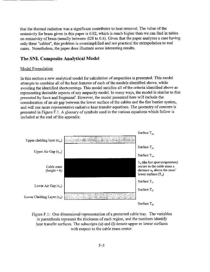
that the thermal radiation was a significant contributor to heat removal. The value of the emissivity for brass given in this paper is 0.92, which is much higher than we can find in tables on emissivity of brass (usually between .028 to 0.6). Given that the paper analyzes a case having only three "cables", this problem is oversimplified and not practical for extrapolation to real cases. Nonetheless, the paper does illustrate some interesting results.

The SNL Composite Analytical Model

Model Formulation

In this section a new analytical model for calculation of ampacities is presented. This model attempts to combine all of the best features of each of the models identified above, while avoiding the identified shortcomings. This model satisfies all of the criteria identified above as representing desirable aspects of any ampacity model. In many ways, the model is similar to that presented by Save and Engmann6. However, the model presented here will include the consideration of an air gap between the lower surface of the cables and the fire barrier system, and will use more representative radiative heat transfer equations. The geometry of concern is presented in Figure F. 1. A glossary of symbols used in the various equations which follow is included at the end of this appendix.

Surface T3,

Upper cladding layer (x) .....

Surface T2, Upper Air Gap (xl•)

Surface T1,

T0 (the hot spot temperature) Cable mass occurs in the cable mass a (height = h) distance x, above the mass'

lower surface (T,1)

Surface T1, Lower Air Gap (x,1

Surface T,1

Lower Cladding Layer (x2,.) - .

Surface T3,

Figure F. 1: One dimensional representation of a protected cable tray. The variables in parenthesis represent the thickness of each region, and the numbers identify

heat transfer surfaces. The subscripts (u) and (1) denote upper or lower surfaces with respect to the cable mass center.

F-5

The model presented here is one-dimensional and conservatively assumes that the heat flow out the sides of the cable tray is negligible. This agrees with assumptions made by Save and Engmann (Ref. 6). For relatively wide cable trays which are uniformly loaded with fully powered cables this is considered an appropriate assumption. However, for cases involving cable diversity questions, this assumption will not apply.

The prediction of heat transfer rates is not exact. That is because the correlations are all derived from experiments which are performed under ideal conditions, and then applied to field applications in which the conditions are largely uncontrolled. For example, the convection experiments are typically limited to very small temperature differences, the ambient conditions are very still, and the geometries are very specific. Typically, twenty percent errors are considered acceptable when applying the ideal experiments to actual geometries. In fact, the same experiment can be performed at two different laboratories and the results vary by this much. So in formulating a model correlations need to be carefully chosen to best represent the problem at hand. The natural convection correlations should also allow for property variations at the elevated air temperatures of concern.

The heat transfer relations will be presented in order from the outside of the geometry towards the inside. The Nusselt number (Nu) is a dimensionless heat transfer coefficient which includes both conduction and convection effects. The first correlation is for the convection off of an upward facing heated horizontal surface (Ref. 9).

Nu =_ 0.54 Ra0 .25 if Ra<10 7 (1) k

Nu = 0.15 Ra 0.333 3 if Ra>10 7

where the Rayleigh number is defined below:

Ra = GO TL3 (2)

The characteristic length, L that is appropriate in Equations I and 2 is half of the width of the cable tray and k is the thermal conductivity of air. From Equation 1 the convective heat flux off of the top surface can be related to the top surface temperature:

q• = h(Tr3u-T 4 ) (3)

F-6

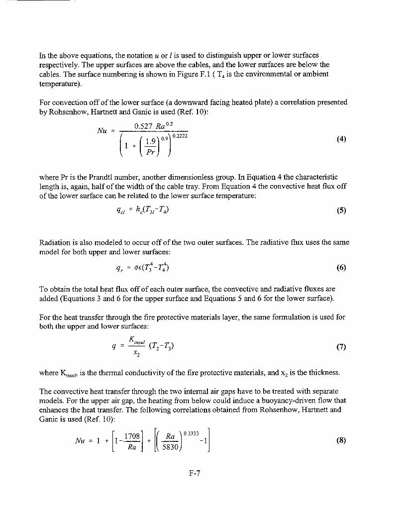
In the above equations, the notation u or 1 is used to distinguish upper or lower surfaces respectively. The upper surfaces are above the cables, and the lower surfaces are below the cables. The surface numbering is shown in Figure F. 1 ( T4 is the environmental or ambient temperature).

For convection off of the lower surface (a downward facing heated plate) a correlation presented by Rohsenhow, Hartnett and Ganic is used (Ref. 10):

Nu = 0.527 Ra 0.2

Pr9 0.9) 0.2222 (4)

where Pr is the Prandtl number, another dimensionless group. In Equation 4 the characteristic length is, again, half of the width of the cable tray. From Equation 4 the convective heat flux off of the lower surface can be related to the lower surface temperature:

qc, = h (T31-T 4) (5)

Radiation is also modeled to occur off of the two outer surfaces. The radiative flux uses the same model for both upper and lower surfaces:

q aq(T -T 4 ) (6)

To obtain the total heat flux off of each outer surface, the convective and radiative fluxes are added (Equations 3 and 6 for the upper surface and Equations 5 and 6 for the lower surface).

For the heat transfer through the fire protective materials layer, the same formulation is used for both the upper and lower surfaces:

q - (T2 -T 3) (7) x2

where KInsul, is the thermal conductivity of the fire protective materials, and x2 is the thickness.

The convective heat transfer through the two internal air gaps have to be treated with separate models. For the upper air gap, the heating from below could induce a buoyancy-driven flow that enhances the heat transfer. The following correlations obtained from Rohsenhow, Hartnett and Ganic is used (Ref. 10):

Nu Ra + I 17081 + [( ) 1 (8)

F-7

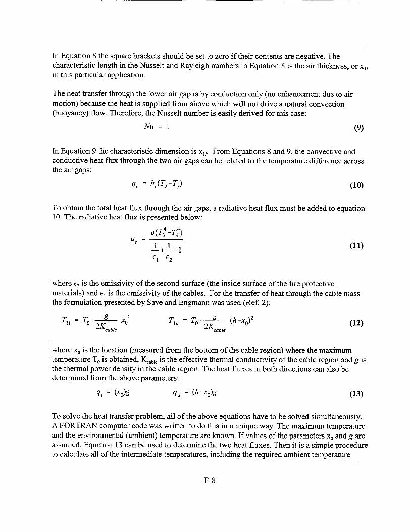
In Equation 8 the square brackets should be set to zero if their contents are negative. The characteristic length in the Nusselt and Rayleigh numbers in Equation 8 is the air thickness, or xit in this particular application.

The heat transfer through the lower air gap is by conduction only (no enhancement due to air motion) because the heat is supplied from above which will not drive a natural convection (buoyancy) flow. Therefore, the Nusselt number is easily derived for this case:

Nu = 1 (9)

In Equation 9 the characteristic dimension is x1l. From Equations 8 and 9, the convective and conductive heat flux through the two air gaps can be related to the temperature difference across the air gaps:

qc = hc(T2 -T 3) (10)

To obtain the total heat flux through the air gaps, a radiative heat flux must be added to equation 10. The radiative heat flux is presented below:

U(T3 -T) qr Iqr=1+ 1 (11)

E I E2

where E2 is the emissivity of the second surface (the inside surface of the fire protective materials) and -1 is the emissivity of the cables. For the transfer of heat through the cable mass the formulation presented by Save and Engmann was used (Ref. 2):

T_ g (h -x 0 )2

Tc a O2K ble XO Tlu = To 2Kcble

where x0 is the location (measured from the bottom of the cable region) where the maximum temperature T. is obtained, Kcable is the effective thermal conductivity of the cable region and g is the thermal power density in the cable region. The heat fluxes in both directions can also be determined from the above parameters:

q, = (Xo)g q, = (h-xo)g (13)

To solve the heat transfer problem, all of the above equations have to be solved simultaneously. A FORTRAN computer code was written to do this in a unique way. The maximum temperature and the environmental (ambient) temperature are known. If values of the parameters x0 and g are assumed, Equation 13 can be used to determine the two heat fluxes. Then it is a simple procedure to calculate all of the intermediate temperatures, including the required ambient temperature

F-8

above and below the tray, using Equations 1 to 12. However, for arbitrary values of x0 and g the environmental temperature will not be reproduced. An optimization routine is used to adjust the x0 and g values so that the environmental temperature is reproduced by calculating in both directions. Since there are two inputs (x0 and g), and two outputs (the environmental temperature at the end of each heat transfer path, i.e. above and below the tray), the solution obtained is unique. The code that is used is presented below.

To determine the cable derating, the ratio of the maximum current allowed for the clad or protected system to maximum current for the baseline or unprotected system must be calculated. To represent the unprotected case, all the thermal resistance factors between upper and lower surfaces 1 and 3 (the cable mass surface and the outer cladding surface both above and below the cable mass as identified in Figure F.1) are set to zero. This can be done by setting their thicknesses to zero, or setting the conductivity of the enclosed materials to infinite.

Example Calculations

Table F. 1 presents the input parameters that are required by the code for the various runs presented here. Some of the cases presented below are divided into sub-cases. These allow for different thicknesses of fire protective materials while keeping the other parameters constant. The code output is also given at the bottom of Table F. 1.

Electrical heating in a cable is generally proportional to the square of current (for a given temperature cable resistance will remain constant). In this case the model is concerned with the overall thermal power associated with the cable mass as a whole, and this is likewise proportional to the square of the individual cable currents. Hence, the ACF is given by the square root of the ratio between the protected and unprotected thermal powers, where the power in each case is that required to raise the maximum cable temperature to 900C:

( '1/2

ACF- g

To calculate the power required without fire protective materials, go, the model given above is run with the resistance values between the air gaps and through the fire protective materials layers set to zero. (This can also be done by setting the gap/material thicknesses to zero.)

Note that the ACF is a secondary output quantity. It is calculated from a ratio of the primary code output which is the allowable heat generation, or total thermal power, level. Even if the model agrees well with experimental measurements of the ACF, if it does not predict reasonable values of the allowable heat generation (equivalent to the square of the cable currents), one would conclude that the model is still in error. That is, the proper basis for evaluation of the model would be based on a comparison of the primary code output (thermal power or currents) to experimental data rather than comparison of the secondary output predictions (ACF).

F-9

Table F. 1: Innut and Outnut for Amnacitv Reduction Calculations

One limitation not resolved by this model is that the determination of the effective conductivity of the cable region is difficult. Estimates are reported in the literature. Engmann (Ref. 2) gives a value of 0.12 BTU/hr-ft.-F for the cable region conductivity and Stolpe (Ref. 1) gives a value 0.15 BTU/hr-ft.-°F. We used 0.14 BTU/hr-ft.-°F as our estimate of this parameter. Our example calculations use a fire protective material with a nominal conductivity of 0.122 BTU/hr-ft.-0 F.

Case 1 tries to reproduce experimental data presented by Save and Engmnann (Ref. 6) Unfortunately they do not give the values for all of the parameters they used. Specifically the depth of the cable region, the size of the lower air gap and the temperature limits are not provided. For this analysis a lower air gap thickness of one-half inch was assumed and values for the other parameters were also assumed based on values that the authors had presented in earlier papers (Refs. 2, 11). The model presented here results in an ACF of 0.73 and 0.67 for the one-half inch and the one inch Thermo-Lag protective barrier systems respectively. This agrees very well with what was found experimentally (0.72 and 0.69 respectively as reported by Save and Engmann, op cit.). Thermal powers, or actual amperage values were not reported, and hence, validation of the primary code output for this case is not possible.

F-10

Case # 1 2 3 4

Inputs h (in) 3.0 3.0 3.0 3.0

x11 (in) 0.2 0.5 0.5 0.5

X1. (in) 0.375 1.0 1.0 1.0

x~i-x 2. (in) 0.0 * 0.0 * 0.0 * 0.0 * 0.5 0.5 0.5 1.0 1.0

Kc.,ij (BTU/F/ft) 0.14 0.14 0.08 0.08

T0 (C) 90 90 90 90

T4 (C) 40 40 40 40

C, 0.8 0.8 0.8 0.8

6C2= 0.9 0.9 0.9 0.9

Output g (BTU/hr/ft3 ) 712 712 525 525 375 354 300 250 318

ACF = (g/g0)" 2 N/A N/A N/A N/A 0.73 6.71 0.76 0.69

1__ _ _ _ 0.67 _ 1_1

a value of zero here indicates the base or unprotected tray case, the remaining values are for different fire barrier thicknesses.

Case 2 represents and attempt to reproduce the thermal powers reported in a recent experimental test report (unpublished Omega Point test for TU, Ref, 3). Table F. 1 shows the initial estimates used to determine the input parameters. The calculated thermal power for the unprotected cable tray using these inputs was found to be 712 BTU/hr-fi.3 as compared to the experimentally measured value of 539 BTU/hr-ft3 . This error was considered significant, and is a source of concern. For the protected case, and even larger relative error between the calculation and the experiment was noted (354 calculated as compared to 216 measured experimentally).

By examining the sensitivity of the model to various parameters, it was found that the thermal conductivity of the cable region strongly affected the unprotected result in particular. In fact, one may suspect that this parameter could vary significantly depending upon the type of cable and density of packing. The Omega Point tests used 3-conductor, 12 AWG, 600 volt cables. The test sample was made with 126 lengths of cable. By adjusting the thermal conductivity of the cable region downward, we were able to reproduce the unprotected cable tray ampacity. Case 3 in Table F. 1 presents these results. However, the modeling results were still significantly in error in predicting the protected case ampacity.

Upon reviewing the pictures taken during the test, it was found that a thermal blanket was placed on top of the cables prior to installation of the fire barrier system (this was consistent with Texas Utilities practice but was not described in the report). The added thermal resistance of this barrier is small if one only considers the extra resistance added by conduction through the blanket. However, the blanket divides the upper air gap into two regions. This adds an extra thermal radiation and convection "cell." This situation is analogous to the difference in the thermal insulation between a double and triple pane window. When the model was extended to include an extra air gap, the agreement between calculation and experiment is significantly improved (a calculated value of 250 compared to the measured value of 216). Case 4 in Table F.1 presents the results for this "extended" case.

This exercise in trying to reproduce experimental results was very educational. It reminds us that heat transfer is typically not an exact science. Experiments to determine standard heat transfer correlations take great pains to make sure that such variations do not influence the results. These extreme measures are not typical in real applications. Therefore, material property and geometry variations in real life applications prevent exact reproduction of experimental data. If a model is to be used to calculate ampacities, then it must be made conservative to allow for as-built variations. And most important, design changes that make the improve the fire protection capability will, in general, adversely affect the ampacity rating.

Conclusions On Ampacity Modeling

A review of the literature on ampacity modeling was conducted. All of the models identified included shortcomings which could be amended. That is, none of the models reviewed was considered to represent an adequate implementation of the current state of heat transfer modeling and understanding. A new horizontal cable tray ampacity model is presented here that combines

F-1I

the best features of the earlier models into a single unified model. (Note that as currently implemented, the model does not consider vertical cable tray configuration nor conduit applications.) The model is one-dimensional, and considered the rates of heat flow from both the upper and lower surfaces of a protected or unprotected cable tray (heat transfer from the sides is neglected). The heat transfer correlations used are based on the appropriate geometric considerations. The model is based on the use of non-dimensional correlations in that all correlations are normalized using non-dimensional groups such as Nusselt, Prandlt, Rayleigh, and Grashof numbers. This simplifies the process of using the model to simulate varying plant conditions, such as cases in which the plant ambient temperature is elevated as compared to the standard test specifications.

One critical and poorly understood parameter identified as a result of these efforts is the effective thermal conductivity of the composite cable mass. Using values reported in the literature, the ampacity model was able to closely match certain experimentally determined ACFs. However, in these initial assessments the primary code output, thermal power, did not match the experimental data. While a reasonable prediction of the thermal power for the protected case was obtained using the nominal parameters discussed above, it was found that only by reducing the cable region thermal conductivity could an adequate match between the calculated and measured unprotected case thermal power values be obtained. Several references to the cable region thermal conductivity were noted, but none of them indicated any experimental measurement technique (these values were reportedly based on experiments although we were unable to identify or retrieve the root source of the reported values). Stolpe estimated a thermal conductivity and retained it because his predicted ampacity was substantiated by an experiment. It now appears that Stolpe, to a certain extent, adjusted the experiments to match his predictions by using a plastic sheet to cover the lower surface of the tray in the testing. Note that Stolpe's model neglected heat transfer from the lower surfaces. This assumption will clearly reduce the ampacity limits and is consistent with the desire to establish conservative bounds on cable performance for the standard ampacity tables. However, for general applications, this simplification is unnecessary and may distort the overall assessment of ACF values.

This illustrates the importance of comparing the predicted and measured thermal powers in addition to the ACF values. It is much easier to match the ACF than the thermal powers since the ACF is a ratio of thermal powers, and hence, small errors in the model will tend to cancel for the ACF. We did note that in many studies inaccuracies are masked because the analysts only compared calculated and measured ACF values instead of the actual heat generation levels.

The source of most of the identified model uncertainties derives from the fact that some input parameters are unknown or highly uncertain (such as the cable thermal conductivity Kcable and many heat transfer coefficients). These uncertainties contribute directly to overall uncertainty in the primary code output, namely, heat loads. It is also noted that the sensitivity of the thermal models to the assumed value of KIable also indicates that actual installations may be sensitive to changes in the cable properties. In particular, the relative volume of cable conductor to cable insulation materials would be expected to significantly impact the net cable mass thermal

F-12

conductivity. This volume ratio would in turn be affected by changes in cable size, multiconductor versus single conductor cables, and changes in cable voltage rating. In general, these would be considered secondary parameters as they will have less impact on the results than will factors such as the type of cable tray tested, how tightly the cables are loaded into the cable tray, and the general nature of the fire barrier system itself.

It should also be recognized that variations in the as-built conditions of the fire barrier system could significantly affect ampacity. For example, parameters of importance would include the presence or absence of air gaps, the actual installed thickness of the material, and overlapping of material. Such factors as the use of protective blankets to protect cables during installation (such as those used by TU for wider cable trays) would also be important ampacity derating considerations. These factors should also be recognized as contributors to uncertainty.

Based on this review it is clear that analytical models need to incorporate significant conservatism in their base formulations, and/or they need to be validated by experiments. In our view, validation is clearly the preferable approach. It was also noted that model validation should be based on a comparison of the primary model output, the cable thermal power, rather than on the more easily matched secondary output (ACF). As noted above, in the formation of the secondary code output, ACF, a ratio of primary code output values is used. In this ratio, certain of the coding errors and uncertainties will tend to cancel. Hence, reliance on validation only through comparison to secondary code output, ACF, could easily lead to a "false sense of security" and an inappropriate conclusion that the primary code output has been validated as well. This situation could easily arise if a model validated for use in the calculation of a relative ACF were used to predict absolute cable ampacity limits for a particular configuration. Such an application would be inappropriate, and might easily lead to erroneous estimates of absolute cable performance limits.

References

1. Stolpe, J. "Ampacities for Cables in Randomly Filled Trays", IEEE Transactions on Power Apparatus and Systems, Vol. PAS-90, Pt. I, pp 962-974, 1971 2. Engmann, G. "Ampacity of Cable in Covered Trays," IEEE Transactions on Power Apparatus and Systems, V PAS-103, n2, pp345-352, Feb. 1984. 3. Omega Point Laboratories, Ampacity Derating of Fire Protected Cables, San Antonio TX, prepared for Texas Utilities Electric Comanche Peak Steam Electric Station, Project number 12340-94583,95165-95168,95246, March 19, 1993. (NOTE: While unpublished, this report was submitted for USNRC review and is available through the USNRC Public Document Room.) 4. Esteves, Oscar M. "Derating Cables in Trays traversing Firestops or Wrapped in Fireproofing" IEEE/ASME/ASCE Joint Power Generation Conference Oct 17-21, 1982. 5. Hiranandani, Ajit K. "Rating Power Cables in Wrapped Cable Trays", IEEE Transactions on Power Delivery, V3, N1, Jan 1988 p7 6 -8 2 . 6. Save, Phil; Engmann, Gary. "Fire Protection Wrapped Cable Tray Ampacity", IEEE Transactions on Energy Conversion V4, n4, December 1989, (manuscript 1987), p5 7 5 -5 84 .

F-13

7. Hiranandani, Ajit "Calculation of Conductor Temperatures and Ampacities of Cable Systems Using a Generalized Finite Difference Model" IEEE Transactions on Power Delivery, V6, n 1, Jan. 1991, pp 15-24. 8. Zhao, Z., Ren, Z. Poulikakos, D. "Heat Transfer in Power Cables packaged inside trays", Journal of Heat Transfer, Transactions ASME, VI 14, n3, Aug. 1992, p7 7 7 -7 8 0 . 9. F. P. Incropera and D. P. DeWitt, Fundamentals of Heat and Mass Transfer, John Wiley &Sons, NY, NY, 1985. 10. W. M. Rohsenow, J. P. Hartnett and E. N. Ganic, Handbook of Heat Transfer Fundamentals, McGraw-Hill Book Co., NY, NY, 1885. 11. Engmann, G., "Cable Ampacity in Trays with Raised Covers," IEEE Transactions on Energy Conversion, V EC-1, n2, pp 113-119, 1986.

Appendix F Nomenclature

Symbol: Definition: g Thermal power or volumetric heat generation rate G Gravitational constant (9.8 m/sec2) h Thickness of cable mass hc Convective heat transfer coefficient k thermal conductivity (general) Kcable Cable mass thermal conductivity KIrl.u Thermal conductivity of fire protective materials Nu Nusselt number Pr Prandtl number q Heat flux (general) qr Heat flux (convective) qr Heat flux (radiative) R Thermal resistanc (general) Ra Rayleigh number T Temperature (general) T4 Temperature (ambient) T,1 Temperature at lower interface n Tnu Temperature at upper interface n To Highest temperature in cable mass x General spatial dimension xn Thickness of layer n x0 Height of cable mass high temperature point relative to bottom of mass a Thermal diffusivity fi Coefficient of thermal expansion 6 Emissivity v Kinematic viscosity (of air) a Stefan-Boltzman constant

F-14

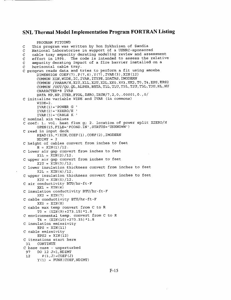
SNL Thermal Model Implementation Program FORTRAN Listing

PROGRAM FITCOND C This program was written by Ron Dykhuizen of Sandia

C National Laboratories in support of a USNRC-sponsored C cable tray ampacity derating modeling review and assessment C effort in 1995. The code is intended to assess the relative

C ampacity derating impact of a fire barrier installed on a

C horizontal cable tray. C program reads data and tries to perform a fit using amoeba

DIMENSION COEF(7),P(7,6),Y(7),IVAR(3),XIN(12) COMMON XIN, WIDE, IC, IVAR, ITYPE, IDATAS, IMODERN COMMON /PARAM/H,XIU,XlL,X2U,X2L,XKO,XKI,XK2,TOT4,EPS,EPS2 COMMON /OUT/QU,QL,ALPHA,BETA,TlL,TlU,T2L,T2U,T3L,T3U,HL,HU CHARACTER*8 IVAR DATA MP,NP,ITER,FTOL,ZERO,IRUN/7,2,0, .00001,0.,O/

C initialize variable WIDE and IVAR (in commons) WIDE=2. IVAR(i)='POWER G I IVAR(2)='XZERO/H I IVAR(3)= CABLE K I

C nominal xin values C coef: 1. vol. heat flux g; 2. location of power split XZERO/H

OPEN(15,FILE='FCOND.IN' ,STATUS='UNKNOWN') C read in input deck

READ(15, *)XIN,COEF(l),COEF(2),IMODERN NDIMT = 2

C height of cables convert from inches to feet H = XIN(1)/12.

C lower air gap convert from inches to feet XlL = XIN(2)/12.

C upper air gap convert from inches to feet XlU = XIN(3)/12.

C lower insulation thickness convert from inches to feet X2L = XIN(4)/12.

C upper insulation thickness convert from inches to feet X2U = XIN(5)/12.

C air conductivity BTU/hr-ft-F XK1 = XIN(6)

C insulation conductivity BTU/hr-ft-F XK2 = XIN(7)

C cable conductivity BTU/hr-ft-F XKO = XIN(8)

C cable max temp convert from C to R TO = (XIN(9)+273.15)*l.8

C environmental temp. convert from C to R T4 = (XIN(1O)+273.15)*I.8

C insulation emissivity EPS = XIN(II)

C cable emissivity EPS2 = XIN(12)

C iterations start here 31 CONTINUE

C base case - unperturbed 97 DO 12 J=l,NDIMT 12 P (1, J) =COEF (J)

Y(1) = FUNK(COEF,NDIMT)

F-15

C perturbed cases to start ameoba search DO 30 I = 1,NDIMT

COEF(I) = COEF(I)*I.005 DO 13 J=1,NDIMT

13 P (I+l, J) =COEF (J) Y(I+l) = FUNK(COEF,NDIMT) COEF(I) =COEF(I)/1.005

30 CONTINUE C call amoeba to perform search

CALL AMOEBA(P,Y,MP,NP,NDIMT,FTOL, ITER) C determine which of the answers is the best

YMIN = 1.E7 NN = NDIMT+l DO 77 I=1,NN

IF(Y(I) .LT.YMIN) THEN C j is index of best answer

J = I YMIN=Y (I) ENDIF

77 CONTINUE C output best solution vector

WRITE(6,881) (P(J,K) ,K=1,NDIMT) 881 FORMAT(' SOLUTION VECTOR FOUND',/,lX,6El3.5) C output cost (should be unity

WRITE (6,99) YMIN C reset guess

DO 98 K=l,NDIMT 98 COEF (K) =P (J, K) 99 FORMAT(' MINIMUM COST ',E13.5)

WRITE (6,61) C it is always a good idea to check answer by repeating calculation C if it is the same no more repeats are required

61 FORMAT(' DO YOU WANT TO CHECK ANSWER, INPUT 1') READ (5, *) ICHK IF(ICHK.EQ.l) GO TO 31 OUTPUT=FUNK (COEF, NDIMT)

C output intermediate temperatures WRITE(6,69)ALPHA,BETA,TIL,TIU,T2L,T2U,T3L,T3U,HL,HU

100 CONTINUE 69 FORMAT(' ',i0(lPEI!.4))

STOP 987 END

C REAL FUNCTION FUNK(COEF,NDIMT)

C code used to solve simultaneous equations C given heat generation rate and xzero, calculate environmental C temperatures -- error is difference between calculated and actual C environmental temperatures C coef 1. volumetric heat flux g 2. location of power split xzero/H

COMMON/PARAM/H, XlU,XlL, X2U, X2L, XKO, XKl, XK2,TO, T4, EPS, EPS2 COMMON/OUT/QU, QL,ALPHA, BETA, TIL, TlU, T2L, T2U, T3L, T3U, HL, HU COMMON XIN, WIDE, IC, IVAR, ITYPE, IDATAS, IMODERN CHARACTER *8 IVAR DIMENSION COEF(7) ,IVAR(3) ,XIN(12)

C parameter alpha ALPHA = 1./COEF(2)-1.

C upper heat flux QU = ALPHA*COEF(i)*COEF(2)*H

F-16

C lower heat flux QL = COEF(l)*COEF(2)*H

C parameter beta BETA = COEF(1)/2./XKO*(H*COEF(2))**2

C conduction through lower cable region -- below xzero TlL = TO - BETA

C convection and radiation through lower air gap FACTOR = 0. CALL PPLATES(TIL,DT,QL,EPS,EPS2,FACTOR,XK1,XlL, IMODERN,WIDE) T2L = TIL - DT

C conduction through lower insulation layer T3L = T2L - QL*X2L/XK2

C convection and radiation to environment -- lower surface HCL = (0.275*(ABS(T3L-T4))**0.3333 )/2. IF (IMODERN.EQ. 1) THEN TAVE = (T3L+T4)/2. CALL PROPS (TAVE, GBNA, PR, XK) RAY = GBNA*ABS(T3L-T4)*(WIDE/2.)**3 HCL= XK*2.*0.527/WIDE*RAY**0.2/(l.+(I.9/PR)**0.9)**.2222 ENDIF HRL = EPS*0.172E-S*(T3L+T4)*((T3L)**2+(T4)**2) HL = HCL +HRL T4L = T3L - QL/HL

C conduction through upper cable region -- above xzero TlU = TO - BETA*ALPHA**2

C convection and radiation through upper air gap C convection between two parallel plates heated from below C use best of conduction or convection to infinite

FACTOR = 1. CALL PPLATES(TIU,DT,QU,EPS,EPS2,FACTOR,XK1,XlU, IMODERN,WIDE) T2U = TlU - DT

C conduction through upper insulation layer T3U = T2U - QU*X2U/XK2

C extra layer of insulation for case 4 C CALL PPLATES(T3U,DT,QU,EPS,EPS2,FACTOR,XK1,XlU, IMODERN,WIDE) C T4U = T3U - DT C TSU = T4U - QU*X2U/XK2 C T3U = T5U C extra layer of insulation C convection and radiation to environment -- upper surface

HCU = 0.275*(ABS(T3U-T4))**0.3333 IF (IMODERN.EQ. 1) THEN

TAVE = (T3U+T4)/2. CALL PROPS (TAVE,GBNA, PR,XK) RAY = GBNA*ABS(T3U-T4)*(WIDE/2.)**3 IF(RAY.LT.1.E7)THEN

HCU = XK*2.*0.54/WIDE*RAY**0.25 ELSE

HCU = XK*2.*0.15/WIDE*RAY**0.3333 ENDIF

ENDIF HRU = EPS*0.172E-8*(T3U+T4)*((T3U)**2+(T4)**2) HU = HCU +HRU T4U = T3U - QU/HU

100 CONTINUE C calculate error

OUTPUT = (T4U-T4)**2+(T4L-T4)**2 FUNK = OUTPUT +1.

F-17

WRITE(6,l)OUTPUT,COEF(l),COEF(2) ,T4L,T4U,QL,QU 1 FORMAT(1 COST 1,7E12.5)

RETURN END

C SUBROUTINE PPLATES (TH,DT,QWANT,EPS1,EPS2, FACTOR, XK, DX, &IMODERN,WIDE) DATA ZERO/0./

C conduction, convection and radiation between parallel plates DT = 1. ICOUNT =0

1 TL =TH-DT C radiation

QRAD = 0.172E-8*(TH**4-TL**4)/(l./EPSl+1./EPS2-1.) C convection

QCONV = 0.275*DT**(1.3333)*FACTOR C conduction

QCOND = DT*XK/DX IF (IMODERN.EQ.1)THEN

TAVE = (TH+TL)/2. CALL PROPS (TAVE,GBNA,PR,XKA) RAY = GBNA*ABS(TH-TL)*(DX)**3 TESTi = l.-1708./RAY IF (TESTl -LT.ZERO) TEST1=ZERO TEST2 = (RA/5830.)**0.3333 - 1 IF CTEST2.LT.ZERO) TEST2=ZERO XXNU = 1.+FACTOR*(TESTl+TEST2) H = XXNtJ*XKA/DX

Cnew H = XKA*0.069/DX*RAY**0.3333*PR**0.074 Cnew QCONV = H*DT*FACTOR

QCONV =H*DT C conduction Cnew QCOND = DT*XKA/DX

QCOND = ZERO ENDIF QI = QRAD+AMAXl (QCOND, QCONV)

C iterate to get downstream temperature CORRECT = QI/QWANT DT = DT/CORRECT TEST = ABSCCORRECT - 1.) IF(TEST.LT.0 .001)RETURN ICOUNT = ICOUNT +1 IF (ICOUNT.GT.500) THEN WRITE (6, 100) TEST,DT

100 FORMAT(' Test,dT 1,2E13.5) STOP 100 END IF GO TO 1 END

C SUBROUTINE PROPS (TEMP. GBNA, PR, XK) DIMENSION RHO(4),PRT(4),TTAB(4),XMU(4),XNUt(4),COND(4)

& , BETA (4) ,AL (4) DATA AL/.646,.720,.905,1.20/ DATA TTAB/0.,32.,1OO.,200./ DATA PRT/0.73,0.72,0.72,0.72/ DATA RHO/.086, .081, .071, .060/ DATA XMU/l .llE-5, 1.165E-5, l.285E-5, l.440E-5/

F- 18

DATA XNU/.130E-3, .145E-3, .180E-3, .239E-3/ DATA COND/0.0133,0.0140,0.0154,0.0174/ DATA BETA/2.18E-3,2.03E-3,1.79E-3,1.52E-3/

C convert to F as per tables from Kreith T = TEMP-460. DO 10 I=2,4

IF(TTAB(I) .GT.T)GO TO 20 10 CONTINUE

I=4 20 FRACT = (T-TTAB(I-1))/(TTAB(I)-TTAB(I-1))

PR = PRT(I-l)+FRACT*(PRT(I) -PRT(I-1)) B = BETA(I-1)+FRACT*(BETA(I)-BETA(I-1)) XN = XNU(I-I)+FRACT*(XNU(I) -XNU(I-1))

C XM = XMU(I-I)+FRACT*(XMU(I)-XMU(I-1)) C R = RHO (I-l) +FRACT* (RHO (I) -RHO (I-l))

XK = CONDT(I-1)+FRACT*(COND(I)-COND(I-1)) A = (AL(I-l)+FRACT*(AL(I)-AL(I-1)))/3600. GBNA = 32.2*B/(A*XN) RETURN END

C SUBROUTINE AMOEBA(P,Y,MP,NP,NDIM,FTOL,ITER)

C subroutine from Numerical Recipes PARAMETER (NMAX=20, ALPHA=l. 0, BETA= 0.5, GAMMIA=2.0, ITMAX=500) DIMENSION P(MP,NP) ,Y(MP) ,PR(NMAX) ,PRR(NMAX) ,PBAR(NMAX) XNDIM = FLOAT(NDIM) MPTS=NDIM+I ITER=0 NDP = NDIM+I

1 ILO=1 IF(Y(1) .GT.Y(2))THEN

IHI=1 INHI=2

C STOP 22 ELSE

IHI=2 INHI=1

C STOP 23 ENDIF DO 11 I=1,MPTS

IF(Y(I) .LT.Y(ILO)) ILO=I IF(Y(I).GT.Y(IHI))THEN

INHI=IHI IHI=I

ELSE IF(Y(I).GT.Y(INHI))THEN IF(I.NE.IHI) INHI=I

ENDIF 11 CONTINUE

RTOL=2.*ABS(Y(IHI) -Y(ILO))/(ABS(Y(IHI))+ABS(Y(ILO))) IF (RTOL. LT. FTOL) RETURN IF(ITER.EQ.ITMAX) PAUSE 'Amoeba exceeding max iterations.' ITER=ITER+1 DO 12 J=I,NDIM

PBAR (J) =0. 12 CONTINUE

DO 14 I=I,MPTS IF (I .NE. IHI) THEN

DO 13 J=1,NDIM

F-19

PBAR(J) =PBAR(J) +P(I,J) 13 CONTINUE

ENDI F 14 CONTINUE

DO 15 J=1,NDIM PBAR (J) =PBAR (J) /XNDIM PR(J) = (.+ALPHA) *PBAR(J)-ALPR*P(IHIJ)

15 CONTINUE IF(NDIM.LT.MP)THEN DO 155 JJ=NDP,MP

155 PR(JJ)=P(1,JJ) ENDI F YPR=FUNK (PR, NDIM) IF(YPR.LE.Y(ILO) )THEN

DO 16 J=1,NDIM PRR(J) =GANMA*PR (J) +(1. -GAMMA) *PBAPR(J)

16 CONTINUE IF (NDIM.LT.MP) THEN DO 165 JJ=NDP,MP

165 PRRJW) =P (1, JJ) END IF YPRR=FUNK (PRR,NDIM) IF(YPRR.LT.Y(ILO) )THEN DO 17 J=1,NDIM

P (IHI, J) =PRR (J) 17 CONTINUE

Y(IHI) =YPRR ELSE

DO 18 J=1,NDIM P (II-I, J) =PR (J)

18 CONTINUE Y(IHI) =YPR

END IF ELSE IF(YPR.GE.Y(INHI) )THEN

IF(YPR.LT.Y(IHI) )THEN DO 19 J=1,NDIM

P (IHI, J) =PR (J) 19 CONTINUE

Y(IHI) =YPR ENDIF DO 21 J=1,NDIM

PRR (J) =BETA*P (IHI, J) +(1. -BETA) *PBAR(J) 21 CONTINUE

IF(NDIM.LT.MP) THEN DO 215 JJ=NDP,MP

215 PRRJW) = P(1, JJ) ENDIF YPRR=FUNK (PRR, NDIM) IF (YPRR.LT.Y(IHI) )THEN DO 22 J=1,NDIM

P (IHI, J) =PRR (J) 22 CONTINUE

Y(IHI) =YPRR ELSE

DO 24 I=1,MPTS IF(I .NE.ILO) THEN DO 23 J=1,NDIM

PR(J)=0.5*(P(I,J)+P(ILO,J))

F-20

P(I,J) =PR (J) 23 CONTINUE

IF (NDIM.LT.MP) THEN DO 235 JJ=NDP,MP

235 PR(JJ)=P(1,JJ) ENDIF Y (I) =FUNK (PR, NDIM)

ENDIF 24 CONTINUE

ENDIF ELSE

DO 25 J=1,NDIM P (IHI, J) =PR (J)

25 CONTINUE Y(IHI) =YPR

ENDIF GO TO 1 END

F-21

Appendix G

Summary of USNRC Reviewed Ampacity Derating Experiments

Introduction

To date, the USNRC has explicitly reviewed fire barrier ampacity derating test results submitted

by three licensees. This appendix provides a brief overview of each of these test programs. Note

that the information is not exhaustive, but rather, is intended to provide an indication of the

nature of the tests performed, and to the extent possible, the results of the test program. In one

case, Florida Power and Light, the USNRC review was based on a proprietary test report. Hence, the discussions provided here are limited to non-proprietary information including a general

description of the test articles and identification of the materials used in testing.

The TVA Watts Bar Testing Progam

TVA tested a fairly wide range of raceways and fire barrier configurations, all involving the fire

barrier material Thermo-Lag (a trademark product of Thermal Science Inc.). Both base (per

original manufacturer specifications) and upgrade (to enhance fire endurance) installations were

tested. The samples tested included single conduits, multiple conduits in a common fire barrier

enclosure, single cable trays, and multiple cable trays in a common enclosure. This test program

is one of the most comprehensive available. The NRC review generally found these tests to be of

high quality, and all were ultimately found acceptable for use in nuclear power plant applications.

The Texas Utilities Electric Testing Program

The test program at Texas Utilities Electric (TUE) also focused on the material Thermo-Lag.

Testing involved single conduits, single cable trays, and air drops (single clad cables). Both base

and upgraded installations were tested. Most tests were found to be of high quality and all were

ultimately accepted. However, note that the results for some conduits were adjusted to reflect

uncertainties in the test results. TUE had used different physical test specimens for certain of the

conduit tests. To address concerns regarding the consistency of the test results, a conservative worst-case ADF was estimated by SNL, and it is this value that is reported here and should be

used in any applications of the TUE data. Note that for these cases, the TVA results include

cases that bound the barrier configurations and do provide more reliable results.

The Florida Power and Light Testing Program

Florida Power and Light (FPL) performed a series of ampacity derating tests involving the materials Thermo-Lag and Darmatt (a Trademark product of Darchem Engineering Inc.) for applications at the Crystal River plant site. The tested configurations involved both conduits and

cable trays. Fire barrier installations tested included each material installed alone and a

combination Thermo-Lag/Darmatt upgrade configuration. However, the USNRC review was

G-1

based on a proprietary test report. Hence, the results of the tests will not be presented here. Readers should consult the public document room or FPL directly for further information on these tests.

Summary of Available Test Results

Table G-l through G-4 provide a summary of the recently completed ampacity derating that have been reviewed and accepted by the USNRC. The results are organized by the type of test article examined. The results include both the TVA and TUE test articles and cover individual conduits (Table G-1), individual cable trays (Table G-2), cable air drops (Table G-3), and special configuration tests (Table G-4).

References

The following is a list of recent ampacity derating test reports that were submitted to and reviewed by the USNRC. These reports are un-published, but are available through the USNRC Public Document Room.

TVA Watts Bar: Testing to Determine Ampacity Derating Factorsfor Fire Protected Cablesfor Watts Bar Nuclear Plant, Central Laboratories Services Report 93-0501, Revision 0, July 6, 1993.

TVA Watts Bar: Ampacity Derating of Cables Enclosed in One-Hour Electrical Raceway Fire Barrier Systems (ERFBS), Omega Point Laboratories Report 11960-97332,97334-6,97768-70, March 28, 1995.

TVA Watts Bar: Ampacity Derating of Cables Enclosed in Cable Tray with Thermo-Lag® 3301/770-1 Upgrade Electrical Raceway Fire Barrier Systems (ERFBS), Omega Point Laboratories Report 11960-97333, June 30, 1995.

TVA Watts Bar: Ampacity Derating of Cables Enclosed in Conduits with Thermo-Lag® 3301/770-1 Upgrade Electrical Raceway Fire Barrier Systems (ERFBS), Omega Point Laboratories Report 11960-97337 & 97338, August 21, 1995.

FPL Crystal River: Ampacity Test Investigation ofRaceway Fire Barriers For Conduit and Cable Tray Systems, Underwriters Laboratory Report Number 95NK17030NC 1973, May 7, 1996. (Note: The USNRC review was based on a proprietary version of this report.)

TUEC Comanche Peak Steam Electric Station: Ampacity Derating of Fire Protected Cables Electrical Test to Determine the Ampacity Derating of a Protective Envelopefor Class JE Electrical Circuits, Omega Point Laboratories, March 19, 1993.

G-2

Tnhko (,-1 Tnjiiviclw'd Cahle Trays Tests Performed As Per IEEE 848 or Similar Standard

ADF Barrier System Source Special Notes

(%)

31.6 lhr T-Lag 330-1 TUE report of - Conducted as per draft 11 of IEEE P848 but did not use 3/19/93 tabulated ampacity for base line;

- included upgrades: increase in material thickness and reinforcing of joints with stress skin; - TU uses a fiberglass blanket over cables to protect them from damage during installation and ADF includes effects of this blanket (used in clad, not in base).

40 lhr T-Lag 330-1 TVA Watts Bar - Included solid steel top cover on tray - nominal 5/8" barrier panels in a single layer

48 3hr T-Lag 330-1 TVA Watts Bar - No Top Cover plus 2x3/8" 770-1 - single 1 1A" layer 330-1 upgrade layers -OPL rpt 11960-97333, item 7.2

Table G-2: Individual Conduit Tests Conducted Per IEEE 848 or Similar Standard

ADF Test Barrier System Source Special Notes Article

9.34% 3/4" Cond. ThermoLag 330- TU report of - TU does not attempt to fill the gap between w/ 3/C #10 1: 1/2" thick 3/19/93 the conduit and the inner surface of the wire conduit sections (Rpt. No. barrier. Hence, there is assumed to be a slight

with additional 12340- gap here. layer of 1/4" 94583, - This may not apply to second layer???

6.67% 2" Cond. thick conduit 95165- - Some tests had inductive heating problems, w/3/C #6 sections 95168, overall not considered significant problem for

95246) this case - Problems noted due to variation in surface

10.7% 5" Cond. ThermoLag 330- properties of conduits used in tests.

w/ 4/C 750 1: 1/2" thick -"350 Top Coat" applied to all

kCMil conduit sections - More conservative results in 21.5-25% range

(w/o the second cited by SNL as bounding uncertainties

1/4" layer)

G-3

Table G-2: Individual Conduit Tests Conducted Per IEEE 848 or Similar Standard

ADF Test Barrier System Source Special Notes I Article I I

5/8" T-Lag

5/8" T-Lag w/ 3/8" upgrade

1/4" T-Lag w/ 1/4" upDrade

1.8% 1" Cond 5/8" T-Lag w/4/C 1

3.3% phase 5/8" T-Lag w/ 3/8" upgrade

1.0% 1/4" T-Lag w/ 1/4" upgrade

(-) 2.7 - 1" Cond. 5/8" T-Lag (-)0.2% w/3/C 3

(-) 0.2 - phase 5/8" T-Lag w/ (+)2.3% 3/8" upgrade

(-) 1.6- 1/4" T-Lag w/ (+) 0.9% 1/4" upgrade

lhr T-Lag 330-1 in sml. box config.

lhr T-Lag 330-1 in Irg. box config

TVA-Watts Bar Report 93-0501, Phase I tests TVA/WBN Phase 2-4 Tests

- preformed conduit sections used - TVA fills gap from conduit to barrier during installation. - TVA used three powering schemes to investigate inductive current problems. Some uncertainty in results - Several tests resulted in an increased ampacity with barrier, hence, negative derating factor (ACF>1.0)

- power source problems of Phase 1 tests not a problem for Phases 2-4 - Also see results for multiple conduits in a common box - small box -41/" square on unistrut frame - large box -30" square on unistrut frame

10% 1" Conduit 3hr T-Lag 330-1 TVA/WBN - 3hr T-Lag is 11/4" pre-formed conduit plus 2x3/8" 770-1 Phase 2-4 sections, upgrade layers Tests - NOT pre-buttered (in contrast to other TVA

13% 4" conduit single conduit tests) only post buttered. - OPL test report 11960-97337 & 97338 items

I 7.6a and 7-6b

G-4

1" Cond w/3/C 1phase

(-)2.7(+)3.5%

(-)0.2(+)4.4%

(-)1.6(+)3.1%

1" Conduit12%

6%

Table G-3: Air Drops

ADF Test Article Barrier System Source Special Notes

21.2% 3/C #6 Air Drop ThermoLag 330-360 TU report of Flexi Blanket: Three 3/19/93 complete wraps with 2

31.8% 750 kCMil Air 4" overlap on each Drop 750 Air wrap staggered 1800 Drop for alt. layers

Table G-4: Special Configurations

ADF Test Article Barrier System Source Special Notes

36% 3-tray stack of 1 hr T-Lag TVA/WBN - For tray stack Top 2 trays powered, standard IEEE Phase 2-4 tests bottom tray no power but full of cables 848 trays -barrier nominal 5/8" panels in a single

layer configuration 8% 1 x3 array of 1" 1 hr T-Lag small -common enclosure for all three trays

conduits box configuration. - for conduits, 1/2*d spacing

26% 2x3 array of I" - small box has panels direct contact

conduits with conduits, large box is about 30" square on unistrut frame.

9% 2x3 array of 1" 1 hr T-Lag large - array given as (vert. x horiz.) conduits box configuration.

G-5

NRC FORM 335 U.S. NUCLEAR REGULATORY COMMISSION 1. REPORT NUMBER (2-89) (Assigned by NRC, Add VoL, Supp.. Rev..

NRCM 1102, BIBLIOGRAPHIC DATA SHEET and Addendum Nunters, if any)

3201,3202 (See instructions on the reverse) NUREG/CR- 6681 SAND2000-1825

2. TITLE AND SUBTITLE

Ampacity Derating and Cable Functionality for Raceway Fire Barriers 3. DATE REPORT PUBUSHED

MONTH YEAR -August 2000

4. FIN OR GRANT NUMBER

JCN J2886 5. AUTHOR(S) 6. TYPE OFREPORT

Steven P. Nowlen Technical 7. PERIOD COVERED (inclusive Dates)

8. PERFORMING ORGANIZATION- NAME AND ADDRESS (if NRc, provide Division, OfficeorRegion, U.S. uc/earRegulatry Commission, and maling address; if contractor, provide narne and mailing address.)

Sandia National Laboratories Mail Stop 0748, PO Box 5800 Albuquerque, NM 87185-0748

9. SPONSORING ORGANIZATION - NAME AND ADDRESS (IfNRC, type 'Sane as above, dconfactor, provideNRCDiision, Office or Region, U.S. NuclearRegulatory Comrmission, and maising address.)

Division of Engineering Office of Nuclear Reactor Regulation U.S. Nuclear Regulatory Comission Washington, DC 20555-0001

10. SUPPLEMENTARY NOTES

R. Jenkins, NRC Project Manager 11. ABSTRACT (200 words or ess)

This report discusses two topical areas associated with localized fire barrier cladding systems for cables and cable raceways; namely, ampacity derating and cable functionality. Ampacity is defined as the electrical current carrying capacity of a particular cable in a given set of routing and environmental conditions. Ampacity derating refers to the process by which cable electrical current carrying limits are reduced in order to compensate for the thermal insulating effects of a raceway fire barrier cladding system. Cable functionality refers to practice of assessing raceway fire barrier fire endurance ratings based on an assessment of the protected cables' ability to perform their intended design function before, during and after the fire endurance exposure. The discussions are based on experience and insights gained through USNRC-sponsored reviews of related licensee submittals. These reviews were conducted between 1994 and 1999 and involved a total of 23 USNRC licensees and numerous individual licensee submittals. In each topical area the report provides general technical background, discusses currently applied methods of assessment and identifies potential technical issues that may arise in the application of each assessment method. The report also provides guidance to assist the USNRC staff in reviewing and assessing licensee submittals in each area.

12. KEY WORDS/DESCRIPTORS (List werds or phrases that will assist researchers in locahng the report.) 13. AVAILABILITY STATEMENT Unlimited

Raceway Fire Barrier 14. SECURITY CLASSIFICATION

Ampacity (This Page)

Derating Unclassified

Fie Endurance (This Rept)

ASTM E119 Unclassified Cable Functionality 15. NUMBER OF PAGES Insulation Resistance

16. PRICE

SNL/6400INRC FormsNRC FORM 335 (2-89)

LpaPrinted on recycled

Federal Recycling Program

UNITED STATES NUCLEAR REGULATORY COMMISSION

WASHINGTON, D.C. 20555-0001

Ampacity Derating and Cable Functionality for - Raceway Fire ...

Documents

Transcript of Ampacity Derating and Cable Functionality for - Raceway Fire ...