ALMA MATER STUDIORUM - UNIVERSITÀ DI BOLOGNA

ALMA MATER STUDIORUM - UNIVERSITÀ DI BOLOGNA

SCUOLADIINGEGNERIAEARCHITETTURA

DIPARTIMENTODIINGEGNERIACIVILE,CHIMICA,AMBIENTALEEDEIMATERIALI

CORSODILAUREAININGEGNERIAPERL’AMBIENTEEILTERRITORIOCurriculum

EARTHRESOURCESENGINEERING

TESIDILAUREA

inOffshoreOil&GasExploitation

Experimental and numerical study of methods to displace oil and water in complex pipe

geometries for subsea engineering

CANDIDATO RELATORE:FrancescoValentini Chiar.moProf.PaoloMacini CORRELATORE Prof.MilanStanko,NTNU,

Trondheim

AnnoAccademico2017/18

SessioneIII

3

AbstractThe purpose of the thesis is to study fluid displacement operations in complex pipe geometries

utilized in offshore petroleum industry. Typically, Monoethylene glycol or Methanol is circulated

through specific sections of the subsea production systems to lower the hydrocarbon content. This is

often done at the beginning of production after a prolonged production shut-in, to avoid formation

of hydrates or to minimize the emissions of chemicals to the environment when a component is to

be replaced.

Experimental and numerical analyses have been conducted modifying a previously built pipe

system formed like a U-shaped jumper, adding a fluid recirculation line, a jet pump, a centrifugal

pump, some new valves and sensors (a flow meter and three pressure sensor). During the

experiments the volume fraction in the U-shaped jumper of the displacing fluid was estimated

versus time by measuring the level of the oil-water interface in each pipe segment. The system was

filled and displaced with both distilled water with 3% water content of salt and Exxsol D60.

Numerical simulations were performed using the one-dimensional transient multi-phase flow

simulator LedaFlow. It has been investigated the necessary displacing time required to achieve

target hydrocarbon concentration in the domain, optimal displacement rate for efficiently removal

of hydrocarbons, and how these variables depend on two different fluids (oil and water) and their

properties. The displacement has been also modelled including or removing the recirculation line.

After carrying out the simulations and performing the experiments, the results were compared, also

against a new simplified mathematical model based on uniform mixing in a tank with the same

volume as the pipe geometry. The results show that there is a fair agreement between the

experimental results, and the results of the simplified model and the LedaFlow simulations. When

including the recirculation line it took longer time to reach the target volume fraction, but the

displacing rate can be lower than when the recirculation line is not present.

4

Preface This Master’s thesis was carried out at the Department of Geoscience and Petroleum Engineering at

the Norwegian University of Science and Technology (NTNU). The thesis is written as the final

part of two years Master’s Programme in “Ingegneria per l’Ambiente e il Territorio”, International

Curriculum “Earth Resources Engineering” (ERE), with specialization in Offshore Engineering at

University of Bologna, Ravenna Campus.

I would like to thank to Professor Paolo Macini, who, together with me, has always believed in this

work, encouraging and helping me when necessary.

I would like to thank to Professor Sigbjørn Sangesland for giving me the opportunity to realize my

Master’s thesis at NTNU, and Professor Milan Stanko for supervising my work and contributing

with important guidance, constantly coordinating my activity. I have always been able to rely on his

valuable advices when I had doubts and problems during the preparation of my thesis.

Moreover, I would like to thank Senior Engineer Noralf Vedvik for helping me in choosing new

devices to assemble, for preparing the new system configuration and for always supporting me with

the system in the lab. The same gratitude is addressed to Senior Engineer Steffen Wærnes Moen for

contributing with the system and the electronics when needed. I also want to thank PhD student

Håvard Skjefstad for his valuable advices during the experiments I have carried in the laboratory of

the Department of Geophysics and Petroleum Engineering of the Norwegian University for Science

and Technology.

Bologna Marzo 2019Francesco Valentini

5

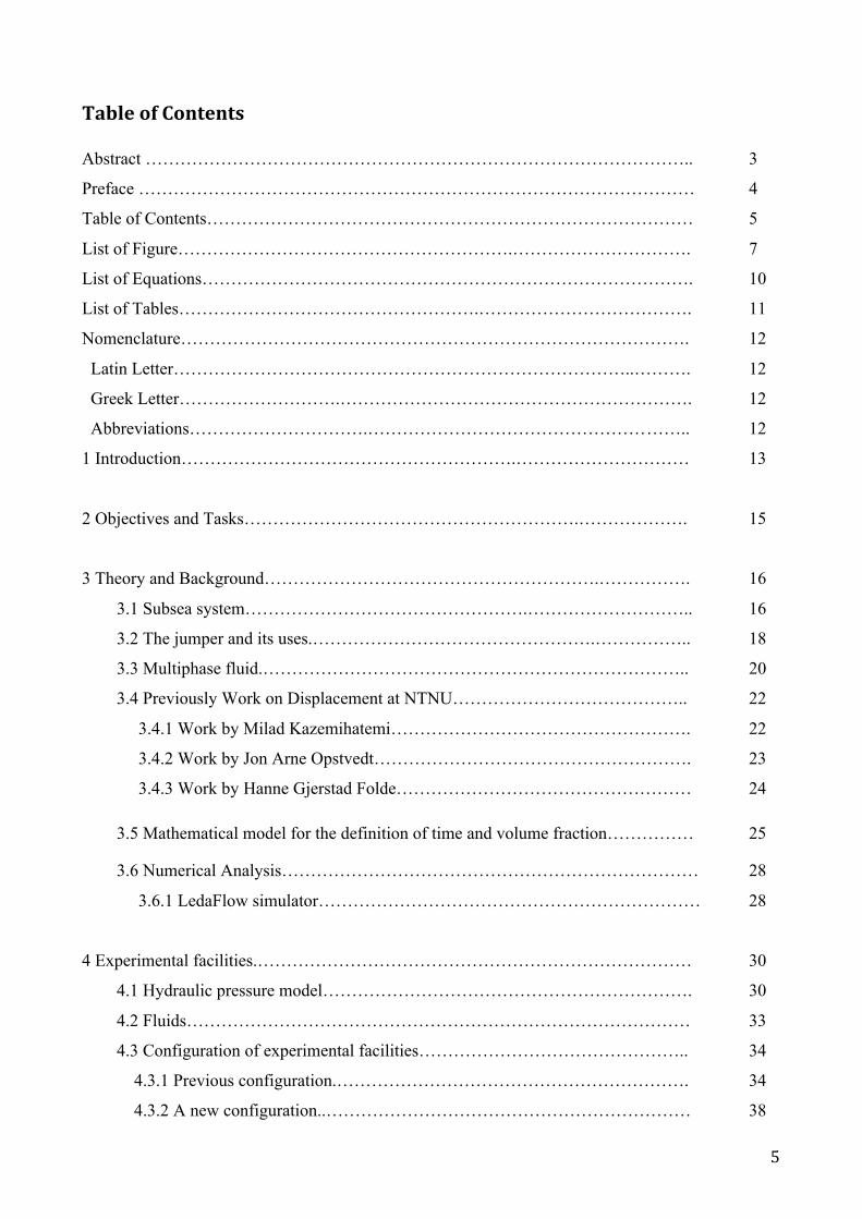
TableofContentsAbstract ………………………………………………………………………………….. 3

Preface …………………………………………………………………………………… 4

Table of Contents………………………………………………………………………… 5

List of Figure………………………………………………….…………………………. 7

List of Equations…………………………………………………………………………. 10

List of Tables…………………………………………….………………………………. 11

Nomenclature……………………………………………………………………………. 12

Latin Letter……………………………………………………………………..………. 12

Greek Letter……………………….……………………………………………………. 12

Abbreviations………………………….………………………………………… …….. 12

1 Introduction………………………………………………….………………………… 13

2 Objectives and Tasks………………………………………………….………………. 15

3 Theory and Background………………………………………………….……………. 16

3.1 Subsea system………………………………………….……………………….. 16

3.2 The jumper and its uses.………………………………………….…………….. 18

3.3 Multiphase fluid.……………………………………………………………….. 20

3.4 Previously Work on Displacement at NTNU………………………………….. 22

3.4.1 Work by Milad Kazemihatemi……………………………………………. 22

3.4.2 Work by Jon Arne Opstvedt………………………………………………. 23

3.4.3 Work byHanne Gjerstad Folde…………………………………………… 24

3.5 Mathematical model for the definition of time and volume fraction…………… 25

3.6 Numerical Analysis……………………………………………………………… 28

3.6.1 LedaFlow simulator………………………………………………………… 28

4 Experimental facilities.………………………………………………………………… 30

4.1 Hydraulic pressure model………………………………………………………. 30

4.2 Fluids…………………………………………………………………………… 33

4.3 Configuration of experimental facilities……………………………………….. 34

4.3.1 Previous configuration.……………………………………………………. 34

4.3.2 A new configuration..……………………………………………………… 38

6

4.4 Jet liquid jet pump……………………………………………………………... 42

4.5 Jet pump model for the case study……………………………………………. 45

4.6 Sensor…………………………………………………………………………. 49

4.6.1 Flow meter……………………………………………………………….. 49

4.6.2 Pressure sensor…………………………………………………………… 50

4.7 Method to determine the volume fraction inside the pipes…………………… 51

5 Numerical simulations with LedaFlow………………………………………………. 54

5.1 General characteristics of the simulations in LedaFlow…………………….. 54

5.2 Geometry and characteristics of the first model…………………………….. 55

5.3 Geometry and characteristics of the new model…………………………….. 58

5.4 LabView .……………………………………………………………………. 61

6 Results.………………………………………………………………………………. 62

6.1 LedaFlow simulation with simple configuration……………………………… 62

6.1.1 Oil displacing water.……………………………………………………. 62

6.1.2 Water displacing oil.……………………………………………………. 64

6.2 LedaFlow simulation with complete configuration…………………………… 66

6.2.1 Oil displacing water …………………………………………………… 66

6.2.2 Water displacing oil……………………………………………………. 68

6.2.3 Analysis of flow rate for water displacing oil…………………………. 70

6.2.4 Effect of the imposed pressure boost for water displacing oil………… 72

6.3 Experiment results for water displacing oil…………………………………. 75

6.4 Comparison of results.………………………………………………………. 80

7 Conclusions………………………………………………………………………… 85

8 References…………………………………………………………………………. 86 9 Appendixes…………………………………………………………………………. 88

Appendix A Method to build a model using LedaFlow simulator……………… 88

7

ListofFigureFigure 3.1: U-shaped jumper in subsea environment…………………………………… 18

Figure 3.2: Flow pattern in case of horizontal oil – water flow………………………… 20

Figure 3.3: Flow pattern in case of vertical oil – water flow…………………………… 21

Figure 3.4: M-jumper used by Kazemihatemi during his experiments………………… 22

Figure 3.5: CAD of the experimental facilities created by Opstveld (2016)…………... 23

Figure 3.6: Oil volume fraction evolution by changing time…………………………… 27

Figure 3.7: Fields used in the 1D model in LedaFlow…………………………………. 29

Figure 4.1: Measures of the U-shaped jumper based on Opstveld (2016)…………….. 34

Figure 4.2: U-jumper with blind flange in the first riser (Opstvedt, 2016)……………. 35

Figure 4.3: U-jumper with the bottom inlet and outlet of the jumper (Opstvedt, 2016).. 35

Figure 4.4: Manifold for pumps (Drawing by Espen Hestdahl)………………………. 36

Figure 4.5: P&ID of the previous configuration (Folde 2017)……………………….. 37

Figure 4.6: Sketch of the new configuration of the flushing rig……………………… 38

Figure 4.7: Detail view of the new configuration of the flushing rig…………………. 39

Figure 4.8: Lateral view of the new configuration of the flushing rig………………… 40

Figure 4.9: Top view of the new configuration of the flushing rig…………………… 40

Figure 4.10: Top view of the new configuration of the flushing rig………………….. 41

Figure 4.10: General view of the new configuration of the flushing rig…………….. 41

Figure 4.12: Jet pump sketch…………………………………………………………. 42

Figure 4.13: Sketch of the jet pump for the created model…………………………… 45

Figure 4.14: Flow meter installed on the flushing rig………………………………… 49

8

Figure 4.15: Meter placed on the pipe for the determination of the volume fraction… 51

Figure 4.16: Sketch of the method for determining the oil volume fraction………… 52

Figure 4.17:Oil column in the vertical part of the jumper……………………………… 53

Figure 5.1: Network of the U-shaped jumper in LedaFlow……………………………. 55

Figure 5.2: U-jumper constructed by Leda Flow simulator……………………………. 57

Figure 5.3: Network of the complete configuration builded in LedaFlow…………….. 58

Figure 5.4: Virtual instrumentation block diagram with LabView……………………… 61

Figure 6.1: LedaFlow results for oil displacing water in simple configuration………… 63

Figure 6.2: LedaFlow results for water displacing oil in simple configuration………… 65

Figure 6.3: LedaFlow results for oil displacing water in complex configuration……… 67

Figure 6.4: LedaFlow results for water displacing oil in complex configuration……… 69

Figure 6.5: Flow rate for water displace oil imposing the same pressure boost of the pump… 71

Figure 6.6: Zoomed view of the first few seconds of the flow rate for water displacing oil..… 71

Figure 6.7: Oil volume fraction with time changing the pressure boost………………… 72

Figure 6.8: Details view for the chart in figure 6.7……………………………………… 73

Figure 6.9: Flow rate with time changing the pressure boost…………………………… 74

Figure 6.10: Details view of the first seconds of the chart in figure 6.9………………… 74

Figure 6.11: Experimental results for water displacing oil……………………………… 76

Figure 6.12: Pipes after 700 seconds injecting 20,77 m3/h when water displacing oil…. 77

Figure 6.13: Experimental flow rate through the jumper for water displacing oil with 5m3/h… 77

Figure 6.14: Experimental flow rate through the jumper for water displacing oil with 10 m3/h 78

Figure 6.15: Experimental flow rate through the jumper for water disp oil with 20,77m3/h… 78

9

Figure 6.16: Comparison results for water displace oil with a flow rate of 5m3/h……… 80

Figure 6.17: Comparison between the complete configuration and experimental results with a flow

rate of 5m3/h……………………………………………………………………………. 81

Figure 6.18: Comparison results for water displace oil with a flow rate of 10m3/h…… 82


rate of 10m3/h………………………………………………………………………… 82

Figure 6.20: Comparison results for water displace oil with a flow rate of 20,77m3/h… 83


rate of 20,77m3/h……………………………………………………………………… 84

Figure 9.1: Graphical User Interface LedaFlow……………………………………… 88

Figure 9.2: Function of the toolbox (KONGSBERG, 2016b)……………………….. 89

Figure 9.3: Graphical User Interface LedaFlow……………………………………… 89

Figure 9.4: Graphical user interface to set characteristics parameters……………….. 90

Figure 9.5: Graphical user interface to set characteristics parameters of the pipes….. 90

Figure 9.6: Phase Split options for mass inlet boundary (KONGSBERG, 2016b)….. 91

Figure 9.7: Phase Split options for pressure boundary (KONGSBERG, 2016b)…… 91

Figure 9.8: Graphical User Interface to set characteristics dimensions of the pipes… 92

10

ListofEquationsEquation 3.1: Volume fraction considering a fluid i…………………………………… 23

Equation 3.2: Mass balance between the incoming mass and the mass exiting the jumper.. 25

Equation 3.3: Oil volume fraction………………………………………………………. 26

Equation 4.1: Haaland equation to determine friction factor…………………………… 31

Equation 4.2: Reynolds Number………………………………………………………… 31

Equation 4.3: Distributed hydraulic pressure losses. …………………………………… 31

Equation 4.4: Concentrated pressure losses……………………………………………... 32

Equation 4.5: Ratio between nozzle area and throat area………………………………. 47

Equation 4.6: Ratio between the primary flow rate and the secondary flow rate………. 47

Equation 4.7: Difference between discharge pressure and throat pressure……………. 47

Equation 4.8: Bernoulli’s theorem to determine throat pressure………………………. 48

Equation 4.9: Discharge pressure………………………………………………………. 48

Equation 4.10:Area occupied by the oil………………………………………………… 52

Equation 4.11: Volume occupied by the oil……………………………………………. 52

11

ListofTablesTable 3.1: Volume fraction results of mathematical model……………………………. 27

Table 4.1: Conditions reproduced in the model………………………………………… 30

Table 4.2: Friction factor based on diameter and Reynolds number…………………… 31

Table 4.3: Total pressure losses in the U-shaped jumper……………………………… 32

Table 4.4: Characteristic parameters of the jet pump model…………………………… 46

Table 4.5: Some result of the jet pump model…………………………………………. 48

Table 5.1: Principal characteristics of the fluid used for the simulations……………… 54

Table 5.2: Characteristics parameter of the PVC pipes………………………………… 55

Table.5.3: Profile of the U-jumper in LedaFlow………………………………………… 56

Table.5.4: Geometry and diameter of U-jumper in LedaFlow…………………………. 56

Table.5.5: Profile of the pipes that make the recirculation line in LedaFlow…………… 59

Table.5.6: Geometry and diameter of the pipes that make the recirculation line in LedaFlow… 59

Table 6.1: Results for the case in which oil displacing water…………………………… 62

Table 6.2: Results for the case in which water displacing oil…………………………… 64

Table 6.3: Results for the case in which oil displacing water in complex configuration.. 66

Table 6.4: Results for the case in which water displacing oil in complex configuration… 68

Table 6.5: Value of the flow rate in the U-shaped jumper for water displacing oil……… 70

Table 6.6: Value of the flow rate in the jumper for water disp oil changing pressure boost 73

Table 6.7: Results from experiment where water is displaced by oil………………….. 75

12

NomenclatureLatinLettersA Area [m2]

D Diameter [m]

f Friction factor [-]

p Pressure [bar]

Q Flow rate [m3/h] / [L/min]

U Voltage

v Velocity [m/s]

V Volume [m3] / [L]

GreekLetters

ρ Density [Kg/m3]

α Volume fraction [-]

ε Absolute roughness [m]

µ Viscosity [Pa s]

σ Interfacial tension [N/m]

Abbreviations1D One dimension

3D Three dimension

CAD Computer-aided design

IGP Institutt for geovitenskap og petroleum

MEG Monoethylene glycol

NTNU Norwegian University of Science and Technology

P&ID Piping and Instrumentation diagram

PVC Polyvinyl chloride

13

1.IntroductionSubsea facilities are playing an increasingly important role in the creation of cost-efficient field

developments. As a means to tackle both new and existing exploration and production challenges,

today's oil and gas projects commonly involve a subsea concept.

It is arguably one of the most important yet technically difficult aspects of the offshore petroleum

industry, but thanks to technological developments and technical expertise, subsea concepts have

become a safe, mature and increasingly cost-effective option for operators looking to address both

existing and new resources.

The underwater drilling and production environment presents unique challenges, particularly deep-

water operations where temperature, pressure and corrosion test the durability of submerged

equipment and tools.

In an offshore field, when temporarily shutting down the production of oil and gas from a well,

there will still be hydrocarbons and water in parts of the subsea system such as flowlines, pipelines

and manifolds.

In recent years, increasingly taking into account environmental, safety and economic factors,

removal of these fluids has been taken into account, in fact constituents of produced petroleum

fluids can be deposited on pipe walls when subjected to cold seawater environment. The depositions

can reduce pipeline hydraulic efficiency and, in severe situations, impede flow. The quality of the

fluids is strongly influenced by the characteristics of each individual site. Certain types of oils, for

example, contain high concentrations of paraffin and waxes dissolved in the oil under reservoir

conditions. In gas/water or gas/oil/water systems, hydrate formation is the main concern. Hydrates

are compounds made up of loosely bonded light hydrocarbon (methane, ethane, and propane) and

water molecules. Hydrate formation is enhanced by cold temperature, high pressure, and

turbulence.

For the reasons explained above, in recent years, strong consideration has been given to removing

these fluids.

One of the best options for moving the fluids that remain in the pipes is through displacement with

a displacing fluid. The displacement process is conducted by injecting another fluid into the system

at a certain rate; the system is circulated for a given time period that should be sufficient to remove

the unwanted fluid.

Sometimes the removal of fluids in these subsea structures is not straight forward, due to

uncertainties regarding displacement volumes and rates. Fluids are often displaced for a longer time

period than necessary, as a consequence this turns out to be expensive. To avoid the problems listed

14

above, the analysis of fluid displacement in pipes is an important field to study in the oil and gas

subsea engineering.

Being able to find the best combination between short time intervals to displaced fluid and a high

efficiency in terms of volume fraction of the fluid displaced is therefore essential.

In the petroleum industry MEG or methanol is commonly used as displacement fluid (Opstvedt,

2016)

There has been conducted some work on the liquid-liquid flow in pipes. One of the first study was

realized by Brauner (2013) that analysed and studied flow patterns and pressure drops in liquid-

liquid flow. However, this study is more directed at the steady-state flow conditions in long pipes.

The research at liquid displacing liquid is more limited, but it is possible to mention Schümann et

al. (2014) who conducted a study on the displacement process through experiments for low flow

rates with simple pipe geometries. Xu et al. (2006) conducted another interesting study, deepening

about diesel oil displacing water to avoid water accumulation in low spots. He executed

experiments with an inclined downhill pipe, considering also a horizontal pipe followed with diesel

oil at low rates to see the displacement effect of water. Cagney et al. (2006) looked into the effect of

methanol injection and gas purging to remove and inhibit water in a jumper. Dellecase et al. (2013)

also studied using methanol and MEG to remove water from the geometry of a jumper.

In 2013 at NTNU Kazemihatami (2013) did his Master’s thesis at NTNU on displacement of

viscous oil in M-shaped jumper using water. During the work realized by Opstveld (2016), both

water displaced by oil and oil displaced water were investigated in a U-shaped jumper at the IGP

Department at Norwegian University for Science and Technology.

In her Master’s thesis at the IGP of Norwegian University for Science and Technology also Hanne

Gjerstad Folde (2017) performed an experimental and numerical study of fluid displacement in

subsea pipe segments. The purpose of this study was to investigate the efficiency of one fluid

displacing another fluid depending on displacement time and velocity in a U-shaped jumper. The

experimental facilities are present in the laboratory of the Department of Geophysics and Petroleum

Engineering at NTNU.

15

2.ObjectivesandTasks

The topic of this Master’s thesis is the “Experimental and numerical study of methods to displace

oil and water in complex pipe geometries for subsea engineering”. The primary objective of this

work is to investigate the efficiency of one fluid given that another fluid is displaced, and

considering as dependent variable the displacement time and velocity. More specifically the focus

will mainly be on the study of liquid-liquid displacement in complex pipe geometries.

The study has been performed through experimental research and numerical simulations.

Experiments have been carried out in a new built pipe system composed by a U-shaped jumper and

a recirculation line with a new liquid jet liquid pump and a new centrifugal pump. The flushing rig

is located at the laboratory hall at the Department of Geoscience and Petroleum at NTNU. In order

to evaluate the displacement process tap water and the synthetic oil Exxsol D60 have been used as

fluids.

In order to obtain realistic simulation models for calculating the displacement efficiency, the

transient multiphase flow commercial simulator LedaFlow has been used. Moreover, the models

created with LedaFlow simulator were compared to the data collected from the experiments and to

the data obtained from the mathematical model, when possible.

The objectives of the project are the following:

• Planning, defining technical requirements, screen suitable components and execute

modifications of the flushing rig already present in the laboratory;

• Contribute in the repair and upgrade of the experimental rig: installation of new centrifugal

pump and a new jet pump, installation of the new pipes which form the recirculation line,

detection and fix of leakages, general maintenance and installation of the second flow meter

and pressure sensor;

• Make a three phase transient 1D numerical model using the commercial simulator

LedaFlow, replacing the displacement process considering a U-shaped jumper and a new

configuration that take into consideration a recirculation line, a centrifugal pump and a

source, useful to simulate the jet pump;

• Validate the model created with LedaFlow, doing some experiments on the flushing rig

present in the IGP laboratory, in order to compare the results.

16

3.TheoryandBackground

3.1Subseasystem

Oil and gas fields, in the quest for reserves, move further offshore into deeper water and deeper

geological formations, therefore the technologies of drilling and production has advanced very

sharply. The continuous increase in the use of these technologies is also due to the fact that the

subsea cost is relatively flat with increasing water depth �(except for the rigid platform case, for

which the costs increase rapidly with water depth). �

The latest subsea technologies have been proven and formed into an engineering system, namely,

the subsea production system, which is associated with the overall process and all the equipment

involved in drilling, field development, and field operation.

A subsea production system consists of several parts that can include a subsea completed well, a

seabed wellhead, a subsea production tree, a subsea tie-in to flow line system, and subsea

equipment and control facilities to operate the well. Such system can range in complexity, varying

from a single satellite well with a flow line connected to a fixed platform, FPSO (Floating

Production, Storage and Offloading), or onshore facilities, to several wells on a template or

clustered around a manifold that transfer to a fixed or floating facility or directly to onshore

facilities.

Moreover, some subsea production systems are used to extend existing platforms. For example, the

geometry and depth of a reservoir may be such that a small section cannot be reached easily from

the platform using conventional directional drilling techniques or horizontal wells. Based on the

location of the tree installation, a subsea system can be categorized either as a dry tree production

system or as a wet tree production system. Water depth can also impact subsea field development.

As a matter of fact, for the shallower water depths, limitations on subsea development can result

from the height of the subsea structures. Christmas trees and other structures cannot be installed in

water depths of less than 30 m (100 ft). For subsea development in water depths less than 30 m (100

ft), situation in which a jacket platforms consisting of dry trees can be used.

The goal of subsea field development is to safely maximize economic gain using the most reliable,

safe, and cost-effective solution available at the time.

Subsea tie-backs are becoming popular in the development of new oil and gas reserves in the 21st

century. In fact, with larger oil and gas discoveries becoming less common, attention has turned to

17

previously untapped, and less economically viable discoveries.

Taking into account a subsea field development, the following issues should be considered:

• Deepwater or shallow-water development; �

• Dry tree or wet tree; �

• Stand alone or tie-back development;

• �Hydraulic and chemical units; �

• Subsea processing; �

• Artificial lift methods; �

• Facility configurations (i.e., template, well cluster, satellite wells, �manifolds).��

18

3.2Thejumperanditsuses

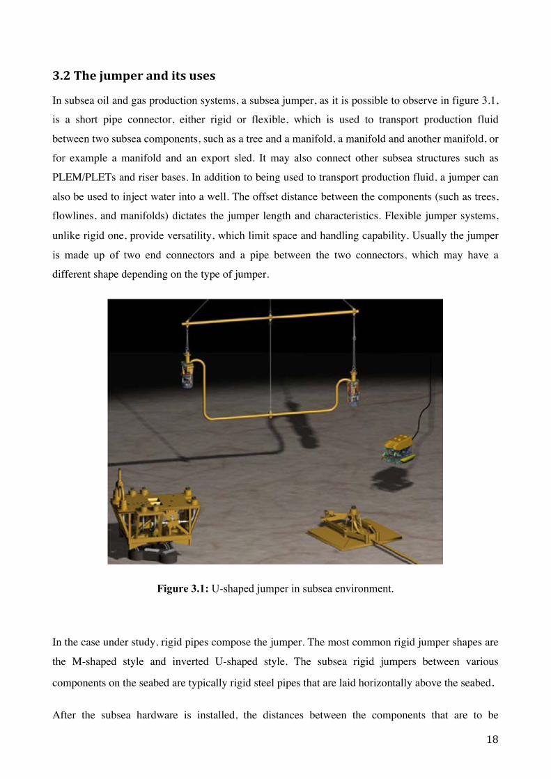
In subsea oil and gas production systems, a subsea jumper, as it is possible to observe in figure 3.1,

is a short pipe connector, either rigid or flexible, which is used to transport production fluid

between two subsea components, such as a tree and a manifold, a manifold and another manifold, or

for example a manifold and an export sled. It may also connect other subsea structures such as

PLEM/PLETs and riser bases. In addition to being used to transport production fluid, a jumper can

also be used to inject water into a well. The offset distance between the components (such as trees,

flowlines, and manifolds) dictates the jumper length and characteristics. Flexible jumper systems,

unlike rigid one, provide versatility, which limit space and handling capability. Usually the jumper

is made up of two end connectors and a pipe between the two connectors, which may have a

different shape depending on the type of jumper.

Figure 3.1: U-shaped jumper in subsea environment.

In the case under study, rigid pipes compose the jumper. The most common rigid jumper shapes are

the M-shaped style and inverted U-shaped style. The subsea rigid jumpers between various

components on the seabed are typically rigid steel pipes that are laid horizontally above the seabed.

After the subsea hardware is installed, the distances between the components that are to be

19

connected are measured. Then the connecting jumper is fabricated to the actual subsea metrology

for the corresponding hub on each component, in which the pipes are fabricated to the desired

length and provided with coupling hubs on the ends for the connection between the two

components. Subsequently, once the jumper has been fabricated, it is transported in situ for the

deployment of the subsea equipment. The jumper will be lowered to the seabed, locked onto the

respective mating hubs, tested, and then commissioned.

20

3.3Multiphaseflow

As already mentioned above a subsea jumper is a short pipe connector used to transport a

multiphase production fluid within an oil and gas production systems.

In recent years multiphase transport receives much attention within the oil and gas industry, in fact

the combined transport of hydrocarbon liquids and gases, immiscible water, and sand can offer

significant economic savings over the conventional platform-based separation facilities. One of the

most common problems is the hydrates formation inside the pipeline that carries the fluids from the

well. It is precisely for this reason that is important to consider the composition of the fluid, the

increasing water content of the produced fluids, erosion, heat loss, and other factors that can create

many challenges to this hydraulic design procedure.

It is possible to define a multiphase flow as a simultaneous passage in a system of a stream

composed of two or more phases. Most of the time, in the oil and gas industry, multiphase flow

consists of three different phases: solids, liquids and gases.

It is clear that the behaviour of a two-phase flow is much more complex than that of single-phase

flow. In fact, a two-phase flow is a process involving the interaction of many variables. The gas and

liquid phases normally do not travel at the same velocity in the pipeline because of the differences

in density and viscosity. For an upward flow, the gas phase, which is less dense and less viscous,

tends to flow at a higher velocity than the liquid phase. For a downward flow, the liquid often flows

faster than the gas because of density differences.

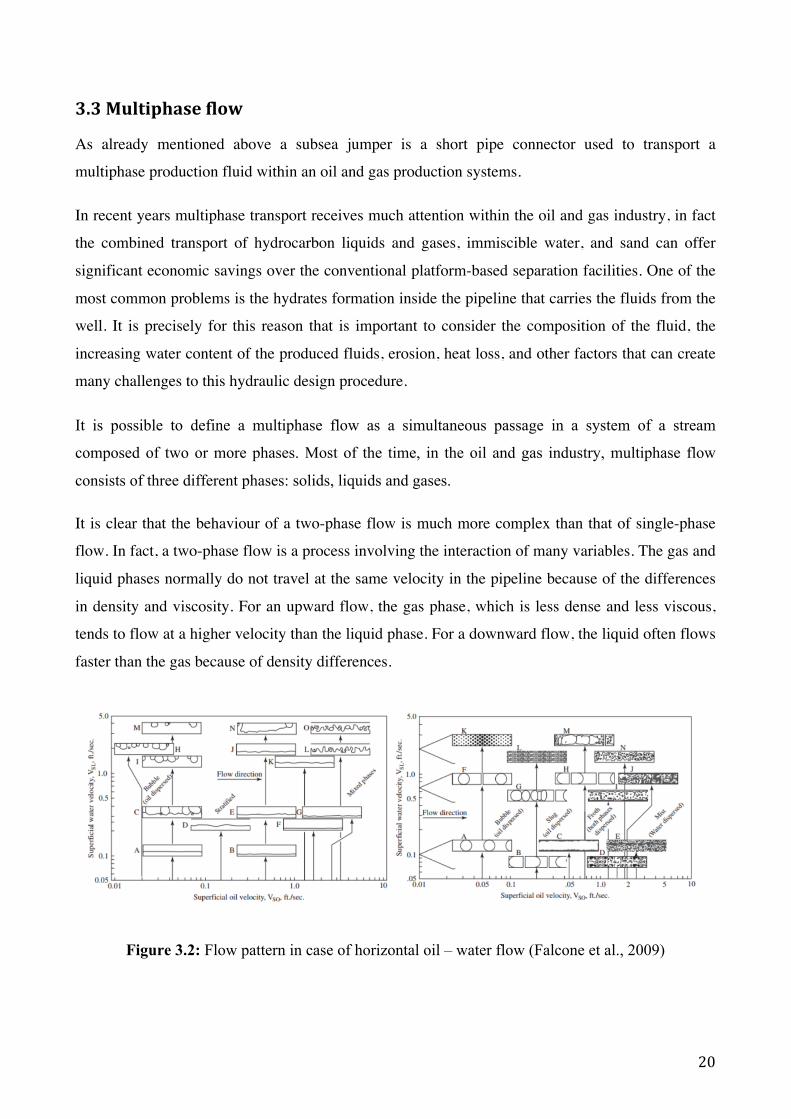
Figure 3.2: Flow pattern in case of horizontal oil – water flow (Falcone et al., 2009)

21

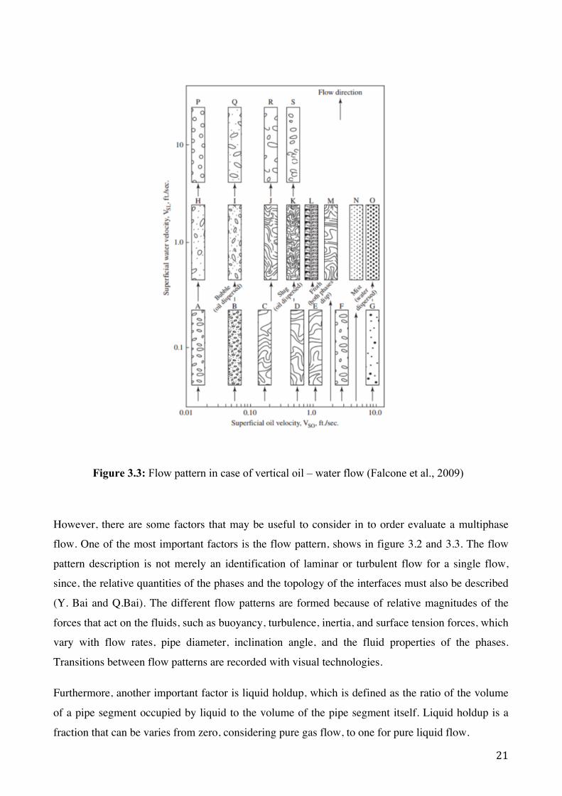
Figure 3.3: Flow pattern in case of vertical oil – water flow (Falcone et al., 2009)

However, there are some factors that may be useful to consider in to order evaluate a multiphase

flow. One of the most important factors is the flow pattern, shows in figure 3.2 and 3.3. The flow

pattern description is not merely an identification of laminar or turbulent flow for a single flow,

since, the relative quantities of the phases and the topology of the interfaces must also be described

(Y. Bai and Q.Bai). The different flow patterns are formed because of relative magnitudes of the

forces that act on the fluids, such as buoyancy, turbulence, inertia, and surface tension forces, which

vary with flow rates, pipe diameter, inclination angle, and the fluid properties of the phases.

Transitions between flow patterns are recorded with visual technologies.

Furthermore, another important factor is liquid holdup, which is defined as the ratio of the volume

of a pipe segment occupied by liquid to the volume of the pipe segment itself. Liquid holdup is a

fraction that can be varies from zero, considering pure gas flow, to one for pure liquid flow.

22

3.4PreviouslyWorkonDisplacementatNTNU

In recent years, other experimental works have been carried out concerning the fluid displacement

inside pipes. Kazemihatami (2013) conducted one of the first interesting studies about fluid

displacement, and afterwards both Opstvedt (2016) and Folde (2017) wrote their Master’s thesis

about displacement process in jumper geometries at the Norwegian University of Science and

Technology in Trondheim. A brief summary of their works and main findings will be presented in

this chapter.

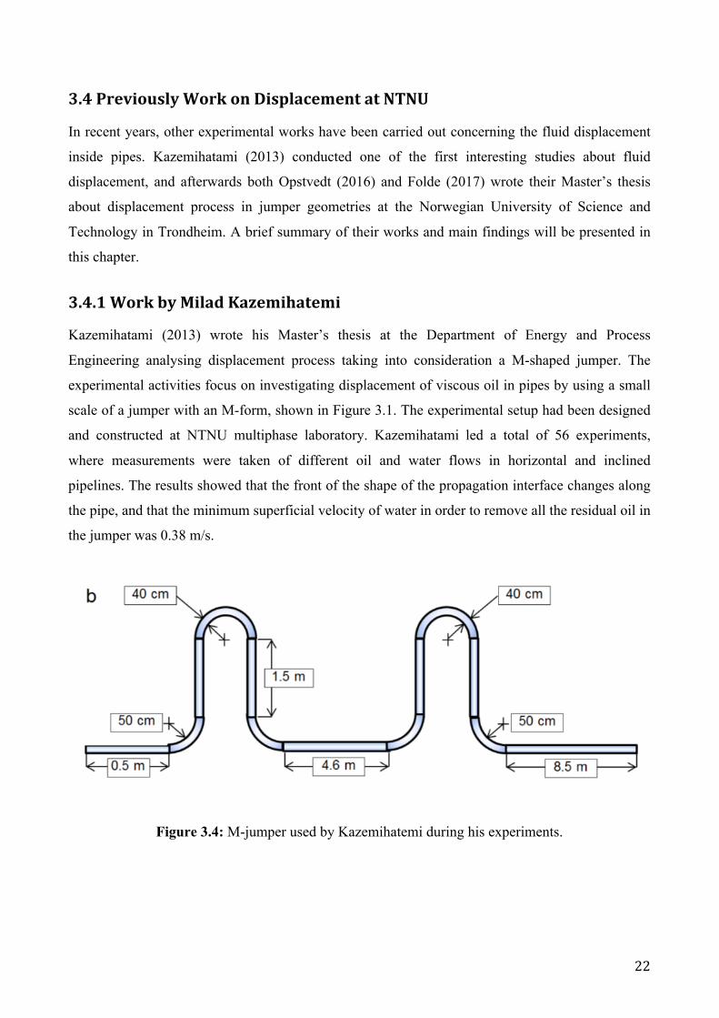
3.4.1WorkbyMiladKazemihatemi

Kazemihatami (2013) wrote his Master’s thesis at the Department of Energy and Process

Engineering analysing displacement process taking into consideration a M-shaped jumper. The

experimental activities focus on investigating displacement of viscous oil in pipes by using a small

scale of a jumper with an M-form, shown in Figure 3.1. The experimental setup had been designed

and constructed at NTNU multiphase laboratory. Kazemihatami led a total of 56 experiments,

where measurements were taken of different oil and water flows in horizontal and inclined

pipelines. The results showed that the front of the shape of the propagation interface changes along

the pipe, and that the minimum superficial velocity of water in order to remove all the residual oil in

the jumper was 0.38 m/s.

Figure 3.4: M-jumper used by Kazemihatemi during his experiments.

23

3.4.2WorkbyJonArneOpstvedt

In his thesis work Opstvedt (2016) conducted an analysis in order to define how the shape of the

displacement front, flow pattern and phase hold up evolve with varying displacement velocities for

a jumper setup. In this case the shape of the experimental facilities was different. In fact as can be

observed from the Figure 3.5 the original jumper built by Opstvedt have a U-shape, different from

the one analysed in the work of Kazemihatemi (2013).

Figure 3.5: CAD of the experimental facilities created by Opstveld(2016).

During the experimentation phase, Opstvedt led a total of 16 experiments using two different

geometries. Both water-oil displacement and oil-water displacement were studied for 4 different

flow rates. The displacement efficiency is defined as the volume fraction of the displacing fluid at a

given time. The volume fraction 𝛼 of a fluid i, is calculated taking into account the ratio between

total volume of fluid i in the domain, and the total volume in the domain as we can observe in the

equation 3.1:

𝛼! =𝑉!𝑉!"!

Equation 3.1: Volume fraction considering a fluid i.

According to what Opstvedt (2016) determined, the displacement efficiency is dependent on the

establishment of a displacement front, which was not clearly observed until flow rates above 20

24

m3/h. Analysing the results obtained in this case study it is possible to affirm that the highest

displacement efficiency was seen for water-oil displacement, even though it was severely reduced

after one displacement volume. Oil-water displacement showed better displacement efficiency after

one volume, but with lower sweep due to reduced front height. In order to provide further detailed

information regarding the multiphase flow dynamics and to examine the accuracy of the numerical

model, numerical simulations were performed. Opstvedt has conducted all the simulation using the

commercially available CFD software ANSYS CFX 16.2, with ANSYS workbench integration. The

simulation domain was meshed using ANSYS ICEM CFD.

3.4.3WorkbyHanneGjerstad Folde The main goal of the thesis developed by Hanne G. Folde (2017) was to investigate the efficiency

of one fluid displacing another fluid (liquid-liquid displacement) depending on displacement time

and velocity.

The study was carried out through experimental research and numerical simulations. The

experimental phase was performed in a previously built pipe system representing a U-shaped

jumper.

The jumper is located at the laboratory hall at the IGP Department of NTNU. Two different fluids

were used to conduct the experiments: tap water and the synthetic oil Exxsol D60. To obtain

realistic simulation models for calculating the displacement efficiency, the transient multiphase

flow commercial simulator LedaFlow was used.

During the experimental phase it was possible to observe a quick and almost linear increase in the

volume fraction of the displacing fluid both for oil displacing water and for water displacing oil,

until approximately one jumper volume was displaced. Moreover, it was also noted that to an

increase in the flow rate of the displacing fluid correspond an increase in the displacement

efficiency, where displacement efficiency is defined as the volume fraction of the displacing fluid.

In terms of flow rate, for oil displacing water, the flow rate 28.16m3/h ± 1.03 m3/h was sufficient

for reaching the criterion of a volume fraction of the displacing fluid above 95 %. It resulted in an

oil volume fraction of 98.0 % ± 0.1 %, after 2.0 volumes displaced. On the contrary, for water

displacing oil the rate 20.77m3/h ± 0.67 m3/h was needed, and resulted in a water volume fraction of

98.6 % ± 0.1 %, after 2.2 volumes displaced.

25

3.5Mathematicalmodelforthedefinitionoftimeandvolumefraction

In order to simulate the displacement process inside the pipes a new mathematical model has been

designed by professor Milan Stanko. The model has been designed to provide results of oil volume

fraction in the case of a two-phase flow consisting water and oil. As will be seen below, however,

the model can also be adapted to a system consisting of a three-phase flow with water, oil and gas.

The mathematical model take into account the balance between the incoming mass and the mass

exiting the jumper considering a reasonable test time. The mass balance in the jumper is:

𝑑𝑚!"!

𝑑𝑡 = 𝑚!" −𝑚!"#

Equation 3.2: Mass balance between the incoming mass and the mass exiting the jumper.

It is possible to express the total mass in the jumper as a function of the volume fractions of the

different phases inside the jumper:

𝑚!"! = 𝑚!"# +𝑚!"# +𝑚!"#$% +𝑚!"#$!!"#$!%&!'

𝑚!"! = 𝑉 (𝛼!"# ∙ 𝜌!"# + 𝛼!"#$% ∙ 𝜌!"#$% + 𝛼!"#$!!"#$%&!' ∙ 𝜌!"#$!!"#$%&!')

The only phase that enters the jumper is the flushing liquid, at a fixed volumetric rate:

𝑚 = 𝑞!"#$!!"#$!%&!'_!" ∙ 𝜌!"#$!!"#$!%&!'

The stream leaving the jumper has the same volumetric rate as the stream entering the jumper:

𝑞!"# = 𝑞!"#$!!"#$!%&!'_!"

The jet pump ensures that there is good mixing of the phases inside the jumper geometry, thus the

stream leaving the jumper will have the same volume fraction values as the total jumper. Whit this

assumption it is possible to write the mass flow of the stream that leaves the jumper as:

𝑚!"# = 𝑞!"#$!!"#$!%&!'_!"(𝛼!"# ∙ 𝜌!"# + 𝛼!"#$% ∙ 𝜌!"#$% + 𝛼!"#$!!"#$%&!' ∙ 𝜌!"#$!!"#$%&!')

Then, substituting these expressions in the jumper mass balance equation and taking into account a

case in which we have only oil and flushing liquid (e.g. water) it is possible to write:

26

𝑑𝑑𝑡 𝑚!"# +𝑚!"# +𝑚!"#$% +𝑚!"#$!!"#$!%&!'

= 𝑞!"#$!!"#$!%&!!!"(𝜌!"#$!!"#!$%!& − 𝛼!"# ∙ 𝜌!"# − 𝛼!"#$% ∙ 𝜌!"#$% − 𝛼!"# ∙ 𝜌!"#

− 𝛼!"#$!!"#$!%&!' ∙ 𝜌!"#$!!"#$!%&!')

𝑉 ∙ (𝑑𝛼!"#𝑑𝑡 ∙ 𝜌!"# +

𝑑𝛼!"#$%𝑑𝑡 ∙ 𝜌!"#$% +

𝑑𝛼!"#𝑑𝑡 ∙ 𝜌!"# +

𝑑𝛼!"#$!!"#$!"#!$𝑑𝑡 ∙ 𝜌!"#$!!"#$!%&!'

= 𝑞!"#$!!"#$!%&!!!"(𝜌!"#$!!"#!$%!& − 𝛼!"# ∙ 𝜌!"# − 𝛼!"#$% ∙ 𝜌!"#$% − 𝛼!"# ∙ 𝜌!"#

− 𝛼!"#$!!"#$!%&!' ∙ 𝜌!"#$!!"#$!%&!')

Considering that:

𝛼!"# + 𝛼!"#$% + 𝛼!"# + 𝛼!"#$!!"#$!%&!' = 1

𝑉 ∙𝑑𝛼!"#𝑑𝑡 ∙ 𝜌!"# − 𝜌!"#$!!"#$!%&!' = 𝑞!"#$!!"#$!%&!!!" ∙ 𝛼!"# ∙ (𝜌!"#$!!"#$!%&!' − 𝜌!"#)

𝑑𝛼!"#𝑑𝑡 = −

𝑞!"#$!!"#$!%&!'_!"𝑉 ∙ 𝛼!"#

Separating variables it is possible to find:

𝑑𝛼!"#𝛼!"#

= −𝑞!"#$!!"#$!%&!'_!"

𝑉 ∙ 𝑑𝑡

Integrating between initial condition and time “t” it is possible to find the a-dimensional value of

the oil volume fraction with the equations:

ln 𝛼!"# !!"# !!!!!!"# ! = −

𝑞!"#$!!"#$!%&!'_!"𝑉 ∙ 𝑡 − 𝑡!

𝛼!"# = 𝛼!"#_!"!#!$% ∙ 𝑒!!!"#$!!"#$!%&!!!"

! ∙(!!!!)

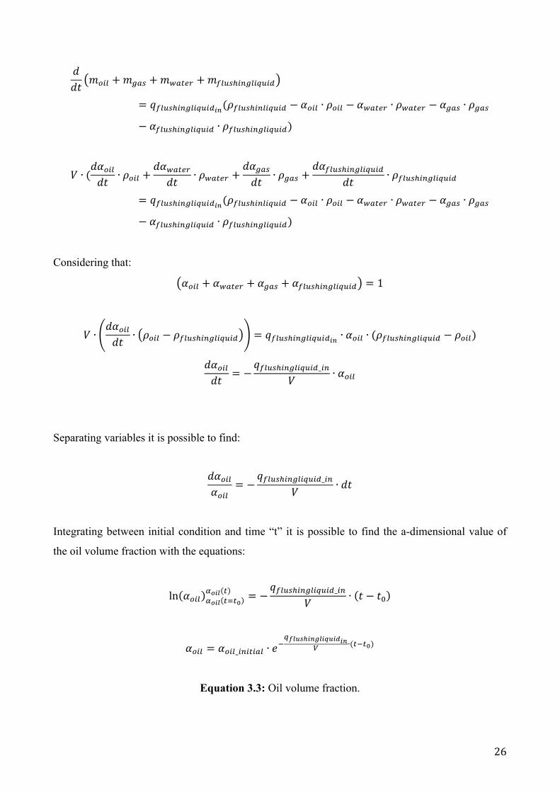
Equation 3.3: Oil volume fraction.

27

By imposing some different value of flow rate (qflushingliquid) the time to have an oil volume fraction

less than 10% was determined and the results are show in the following table.

Flowrate Time Oilvolumefraction Watervolumefractionm3/h s [-] [-]2 960 0,09938 0,900623 640 0,09938 0,900625 384 0,09938 0,900628 240 0,09938 0,9006210 192 0,09938 0,9006213 148 0,0989 0,901115 128 0,09938 0,9006218 108 0,09655 0,90345

20,77 96 0,09096 0,90904

Table 3.1: Volume fraction results of mathematical model

From the results presented in the table and from the figure 3.3 it is possible to state that, by

increasing the speed, the displacement time necessary to reach a value of less than 10% of oil

volume fraction decreases. In particular, figure 3.6 shows the oil volume fraction evolution for

different imposed value of flow rate with time. The displacement efficiency is defined as the

volume fraction of the displacing fluid at a given time.

Figure 3.6: Oil volume fraction evolution by changing time.

00,10,20,30,40,50,60,70,80,91

0 100 200 300 400 500 600 700 800 900 100011001200

Oilvolumefractio[-]

time[s]

Oilvolumefractionevolutionbychangingtime

20,769m^3/h

18m^3/h

15m^3/h

13m^3/h

10m^3/h

8m^3/h

5m^3/h

3m^3/h

2m^3/h

28

3.6NumericalAnalysis

To simulate the movement of a multi-phase fluid, there are several commercial software available

on the market. One may choose between the 1D simulator tools LedaFlow by KONGSBERG and

OLGA by Schlumberger, or the 3D computational fluid dynamic tool ANSYS CFX. LedaFlow is a

transient multiphase flow simulator, based on multiphase physics from large-scale experiments and

gathered field data. Transient simulation with the OLGA simulator provides an added dimension to

steady-state analyses by predicting system dynamics such as time-varying changes in flow rates,

fluid compositions, temperature, solids depositions and operational changes.

The CFD software is governed by physical laws, and applied through averaged Navier-Stokes

equations along with models for phase interaction and turbulence (Opstvedt, 2016). In the present

work, LedaFlow will be explored as a tool for simulating displacement, and compared to the models

made with the same simulator by Folde 2017.

3.6.1LedaFlowsimulator

LedaFlow is the product of ten years of innovative development by SINTEF sponsored, guided and

supported by important sector leader such as TOTAL and ConocoPhillips. This software is

marketed and developed further by KONGSBERG.

LedaFlow is based on models that are closer to the actual physics of multiphase flow and provides a

step change in detail, accuracy and flexibility over existing multiphase flow simulation technology.

The software has been validated against the best available and most comprehensive experimental

data sets to ensure that the models are as best representative as possible and is designed with an user

interface, which is easier and more intuitive to use.

Two models are included in LedaFlow: the Point model and the 1D model.

The Point model is used for “one point” of all the three flow cases; single, 2-phase (liquid and gas)

and 3-phase to solve steady state equations. It is assumed that there exists a thermodynamic

equilibrium, which means no compositional effects are taken into account when the fluid

distribution is computed. The mixture temperature is giving the foundation of the temperature

distribution. In the Point model a fast and steady state solution with exact mass conversion is

reached, and is the basis of the steady-state pre-processor for 1D transient code.

The other model, 1D model, is used for transient situations for the same three flow cases. In the

field approach from LedaFlow there is included a detailed modelling of water and oil dispersions

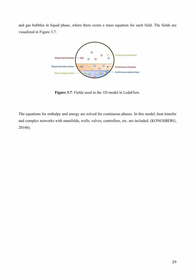
29

and gas bubbles in liquid phase, where there exists a mass equation for each field. The fields are

visualized in Figure 3.7.

Figure 3.7: Fields used in the 1D model in LedaFlow.

The equations for enthalpy and energy are solved for continuous phases. In this model, heat transfer

and complex networks with manifolds, wells, valves, controllers, etc. are included. (KONGSBERG,

2016b).

30

4.Experimentalfacilities

This chapter first describes the type of fluids used for the realization of the simulations phase (made

by LedaFlow simulator) and experiments in the laboratory. After this part there is a description of

the previous configuration of the flushing rig and a description of the new configuration, which is

the subject of study of this master’s thesis. The last part is about the creation of numerical models in

LedaFlow.

4.1Hydraulicpressuremodel

In order to understand and predict the possible pressure losses inside the pipe system can be, a

model has been created. The starting flow rate is 13m3/h.

The model has been created for 3 different configurations: a first configuration in which the jumper

is completely filled with oil, in this phase the maximum oil volume fraction and a fraction equal to

0 of water was considered (the density and viscosity of the oil have been taken into consideration),

an intermediate configuration during which the displacement process is underway and so the water

volume fraction and the oil volume fraction are considered the same, and a third phase in which the

water almost completely displaced oil, therefore it is possible to find a high value of water volume

fraction and a very low quantity of oil inside the jumper.

Starting conditions Transitional conditions Final conditions

Water volume fraction [-] 0 0,5 0,902 Oil volume fraction [-] 1 0,5 0,098 Water density Kg/m3 998,9 998,9 998,9

Oil (ExxolD60) density Kg/m3 786 786 786 Total density kg/m3 786,00 892,45 978,04

Viscosity Pa s 0,00156 0,00133 0,001095

Table 4.1: Conditions reproduced in the model

A fluid flowing inside a pipe is subject to the so-called distributed pressure losses, a pressure drop

due to the internal friction. A fundamental parameter for the definition of pressure losses is the

friction coefficient, in this circumstance determined with the Haaland formula.

Professor S.E. Haaland of the Norwegian Institute of Technology (NTNU) proposed the Haaland

equation in 1983. It is used to solve explicitly for the Darcy-Weisbach friction factor f for a full-

31

flowing circular pipe. It is an approximation of the implicit Colebrook–White equation, but the

discrepancy from experimental data is well within the accuracy of the data.

The Haaland Formula is:

1𝑓= −1,8 𝑙𝑜𝑔

𝜖𝐷3,7

!,!!

+6,9𝑅𝑒

Equation 4.1: Haaland equation to determine friction factor.

In the previous equation “Re” is the Reynolds number determined by the equation:

𝑅𝑒 =𝑣𝐷𝜌𝜇

Equation 4.2: Reynolds number.

The result of the calculation useful to determine the friction factor are expressed in the table below:

Friction factor - Haaland equation Roughness (m) Diameter (m) Re Friction factor

0,0000015 0,153 26854,7 0,3934 0,0000015 0,16 25679,8 0,3944

Table 4.2: Friction factor based on diameter and Reynolds number

The distributed pressure losses have been determined with the formula:

∆𝑃 = 𝑓𝐿𝐷𝑣!

2 𝜌

Equation 4.3: Distributed hydraulic pressure losses.

Where:

• f is the friction factor determined with Haaland Equation.

• L is the length of the pipe expressed in meters;

• D is the diameter of the pipe expressed in meters;

• v is the velocity determined by the ratio of the imposed flow rate (m3/h) and the area of the

pipes (m2).

• ρ is the density of the fluid expressed in Kg/m3.

32

In the event that the fundamental cause of dissipation is given by the geometric configuration or the

presence of any accidentality, such as bends, elbows, valves, faucets, we will have pressure losses

called concentrated. This denomination depends on the fact that they are located in precise points of

the conduit and not distributed along the entire length of the tube.

In the experimental facilities there are also elbows and it is therefore important to determine the

concentrated pressure losses.

The formula employed is:

Δ𝑃 = 𝛽𝑣!

2 𝜌

Equation 4.4: Concentrated pressure losses.

The term β, which correspond to the friction coefficient, depends on the particular geometry of the

object that determines the loss, and is tabulated. In the event of a loss due to the presence of a 90°

elbow the value of β is equal to 0,9 and it is dimensionless.

Length of the pipes (m) Diameter (m) Re Friction factor ΔP (bar)

Section 1 1 0,153 26854,7 0,3934 0,0005 Elbow 1 0,16 25679,8 0,3945 0,0001 Section 2 1,6 0,153 26854,7 0,3934 0,0008 Elbow 2 0,16 25679,8 0,3945 0,0001 Section 3 1,536 0,153 26854,7 0,3934 0,0007 Elbow 3 0,16 25679,8 0,3945 0,0001 Section 4 1,5 0,153 26854,7 0,3934 0,0007 Elbow 4 0,16 25679,8 0,3945 0,0001 Section 5 3 0,153 26854,7 0,3934 0,0015 Elbow 5 0,16 25679,8 0,3945 0,0001 Section 6 2 0,153 26854,7 0,3934 0,0010 Elbow 6 0,16 25679,8 0,3945 0,0001 Section 7 0,3 0,153 26854,7 0,3934 0,0001 Elbow 7 0,16 25679,8 0,3945 0,0001 Section 8 2,1 0,153 26854,7 0,3934 0,0010 Elbow 8 0,16 25679,8 0,3945 0,0001 Section 9 1 0,153 26854,7 0,3934 0,0005 Total ΔP 0,0080

Table 4.3: Total pressure losses in the U-shaped jumper

Observing the values included in the table 4.3 it is possible to state that the total pressure drops are

very low, due above all to the friction of the fluid on the walls of the pipes and to the losses

concentrated in the elbows.

33

4.2Fluids

Both for the simulation phase with LedaFlow simulator and for the following experimentation

phase in the laboratory, tap water and oil Exxol D60 (produced by ExxonMobil Chemicals) were

used.

During the testing phase, to reduce the possibility of errors due to changes in the intrinsic properties

of the fluids used, the characteristic parameters of tap water and oil Exxsol D60 have to be the

same. In this case the properties of the oil remain unchanged, while the properties of water can

change day by day or may vary from place to place. Since the experiments were carried out in a

single week, it can be assumed that the properties of the water remain unchanged.

Certainly it would have been better to use crude oil in order to simulate a closer case-study to a real

situation of deposit, but due to the fact that it is not easy to find this material on the market, and take

into account its toxicity, Exxol D60 oil was used. In fact, this product has values similar inherent

characteristics parameters comparable with real ones.

Exxsol D60 Fluid is produced from petroleum-based raw materials, which are treated with

hydrogen in the presence of a catalyst to produce a low odour, low aromatic hydrocarbon solvent.

The major components of this product include normal paraffin, isoparaffins, and cycloparaffins.

Reading the product specifications from ExxonMobil (2005) one can see that the viscosity at 25 °C

is 1.43 mPa s. Due to high temperatures, real crude oils might actually exhibit viscosities similar to

the Exxsol D60. The interfacial tension between water and Exxsol D60 has been measured to 36

mN/m in 2016 by SINTEF, using a Pendant Drop measurement method with a Teclis Tracker

tension meter from Teclis Instruments (Fossen, 2016).

Exxsol D60 Fluid is generally recognized to have low acute and chronic toxicity. Vapour or aerosol

concentrations above the exposure limit of 184 parts per million (ppm) in the air can cause eye and

lung irritation and may cause headaches, dizziness or drowsiness. Prolonged or repeated skin

contact in an occupational setting may result in irritation so for this reason, during the laboratories

activity, all appropriate security measures have always been used (use of chemical resistant gloves

and glasses is recommended). Exxsol D60 fluid is not regarded as a mutagen or carcinogen, and

there is low concern for reproductive, developmental, or nervous system toxic effects.

In order to distinguish between the transparent liquids, Exxsol D60 and water, the oil was dyed with

“Oil Red O” color powder. The Oil Red O color powder does not affect the surface tension of the

oil (Chen et al., 2016).

34

4.3Configurationofexperimentalfacilities

This chapter makes an excursus explaining the previous configuration and all the changes that have

been made to it to arrive at a new configuration of the flushing rig. Below we will deepen the

characteristics of the new devices that have been purchased and mounted on the new flushing rig.

The characteristics of the new jet pump are also described below. In order to purchase the best

product according to our technical requirements, a model has been created specifically for this case

study. In detail below the characteristics of the flow meters and pressure sensors installed in the

new model of flushing rig were described.

4.3.1PreviousConfiguration

The previous configuration of the U-shaped jumper used by H. Folde (2017) in her thesis is the

same as built by Opstvedt (2016).

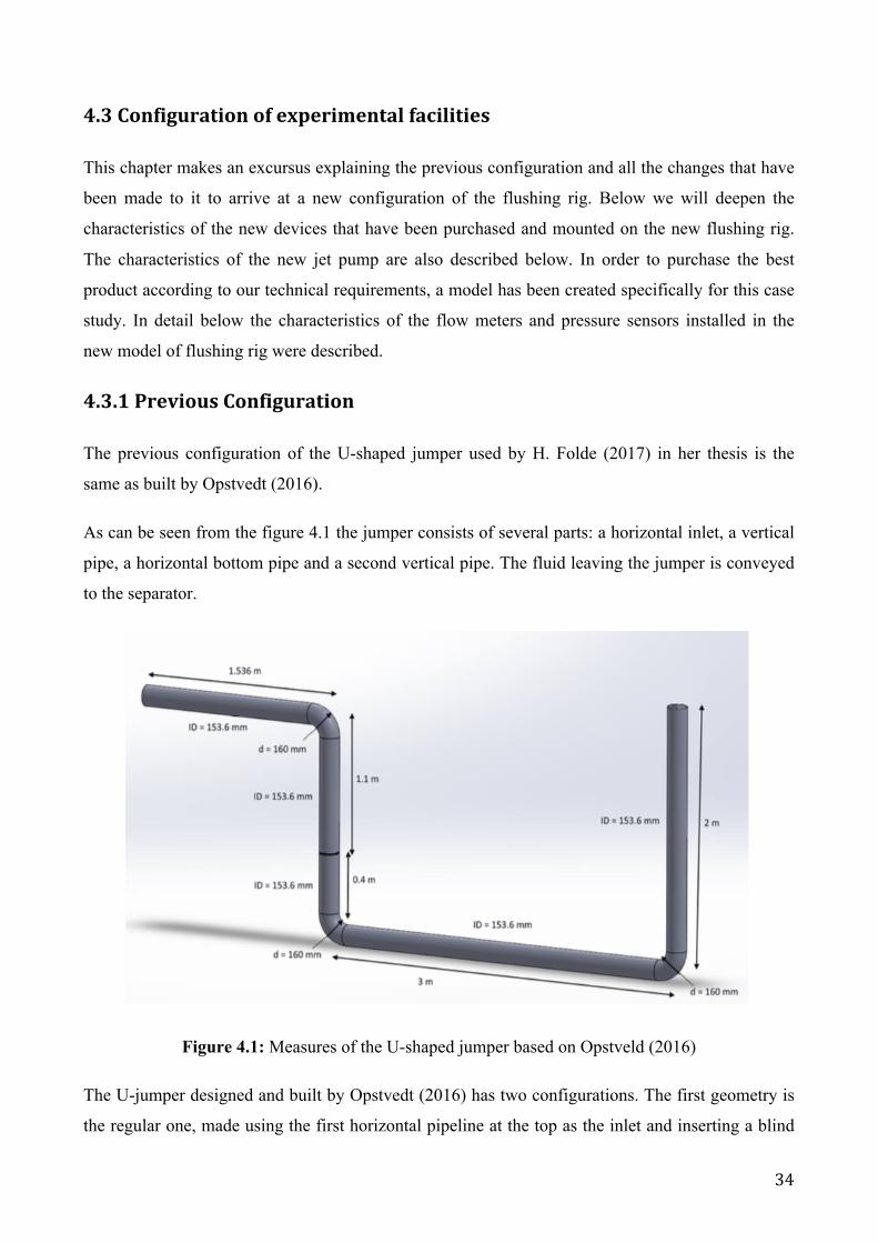
As can be seen from the figure 4.1 the jumper consists of several parts: a horizontal inlet, a vertical

pipe, a horizontal bottom pipe and a second vertical pipe. The fluid leaving the jumper is conveyed

to the separator.

Figure 4.1: Measures of the U-shaped jumper based on Opstveld (2016)

The U-jumper designed and built by Opstvedt (2016) has two configurations. The first geometry is

the regular one, made using the first horizontal pipeline at the top as the inlet and inserting a blind

35

flange in the first riser, as shown in Figure 4.2 (Opstvedt, 2016). Then the whole volume of the

jumper is investigated.

Figure 4.2: U-jumper with blind flange in the first riser (Opstvedt, 2016)

Unlike the first, for the second geometry an extra inlet is built, shown as the bottom inlet in Figure

4.3 (Opstvedt, 2016). When the first riser is cut off, this gives the possibility of studying

displacement in a closed off section.

Figure 4.3: U-jumper with the bottom inlet and outlet of the jumper (Opstvedt, 2016)

36

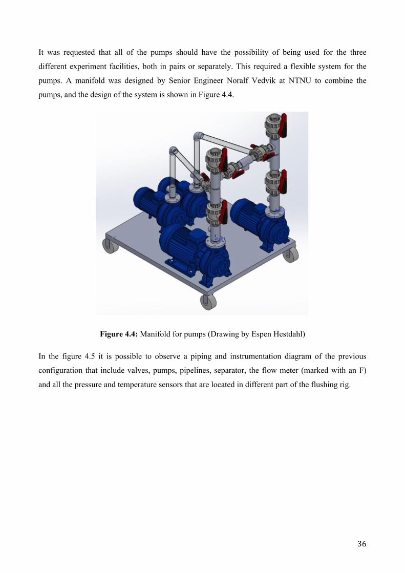
It was requested that all of the pumps should have the possibility of being used for the three

different experiment facilities, both in pairs or separately. This required a flexible system for the

pumps. A manifold was designed by Senior Engineer Noralf Vedvik at NTNU to combine the

pumps, and the design of the system is shown in Figure 4.4.

Figure 4.4: Manifold for pumps (Drawing by Espen Hestdahl)

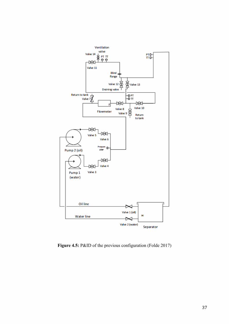
In the figure 4.5 it is possible to observe a piping and instrumentation diagram of the previous

configuration that include valves, pumps, pipelines, separator, the flow meter (marked with an F)

and all the pressure and temperature sensors that are located in different part of the flushing rig.

37

Figure 4.5: P&ID of the previous configuration (Folde 2017)

38

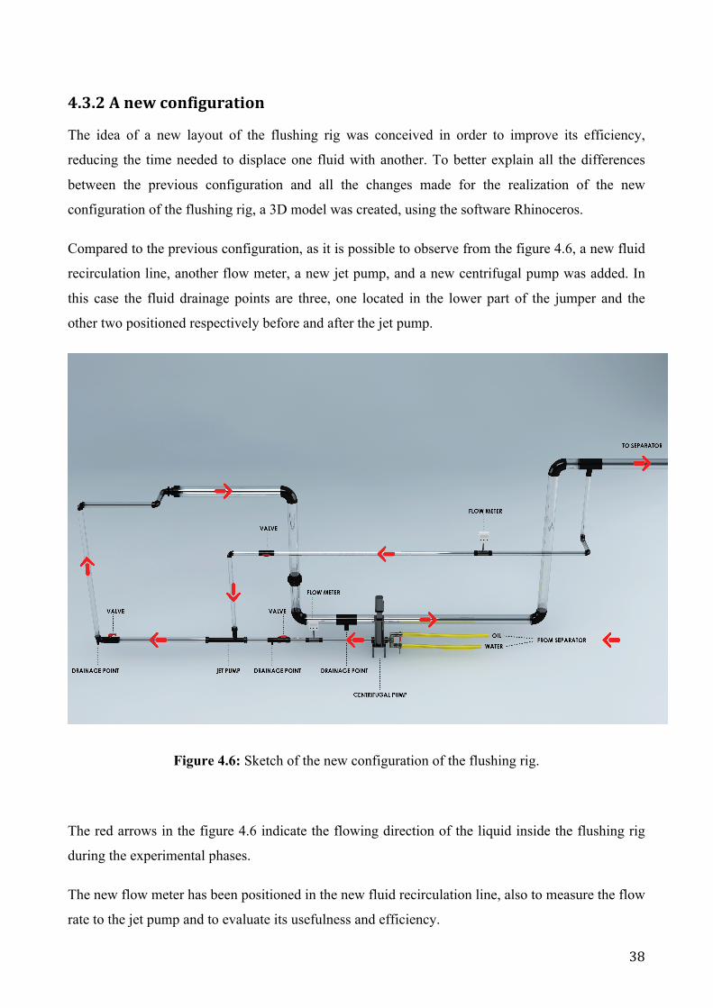
4.3.2Anewconfiguration

The idea of a new layout of the flushing rig was conceived in order to improve its efficiency,

reducing the time needed to displace one fluid with another. To better explain all the differences

between the previous configuration and all the changes made for the realization of the new

configuration of the flushing rig, a 3D model was created, using the software Rhinoceros.

Compared to the previous configuration, as it is possible to observe from the figure 4.6, a new fluid

recirculation line, another flow meter, a new jet pump, and a new centrifugal pump was added. In

this case the fluid drainage points are three, one located in the lower part of the jumper and the

other two positioned respectively before and after the jet pump.

Figure 4.6: Sketch of the new configuration of the flushing rig.

The red arrows in the figure 4.6 indicate the flowing direction of the liquid inside the flushing rig

during the experimental phases.

The new flow meter has been positioned in the new fluid recirculation line, also to measure the flow

rate to the jet pump and to evaluate its usefulness and efficiency.

39

The new centrifugal pump is a vertical, multistage pump with suction and discharge ports at the

same level (in-line) enabling installation in a horizontal one-pipe system. The pump is fitted with a

3-phase, fan-cooled, permanent magnet, synchronous motor. The motor includes a frequency

converter and PI controller in the motor terminal box. This enables continuously variable control of

the motor speed, which again enables adaptation of the performance to a given requirement.

In the experiments, all pipes in the figure were filled initially with the fluid to be displaced with the

aid of the centrifugal pump that draws the liquid directly from the separator. After that, the pump

was turned off and the valves in the pump suction manifold were closed and open to select the

source of the displacing fluid (if, for example, the tube was filled with oil the oil valve was closed

and the valve opened allowing water to flow into the system).

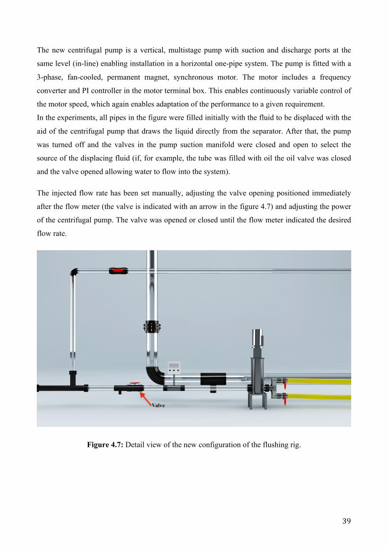
The injected flow rate has been set manually, adjusting the valve opening positioned immediately

after the flow meter (the valve is indicated with an arrow in the figure 4.7) and adjusting the power

of the centrifugal pump. The valve was opened or closed until the flow meter indicated the desired

flow rate.

Figure 4.7: Detail view of the new configuration of the flushing rig.

40

Figure 4.8: Lateral view of the new configuration of the flushing rig.

Figure 4.9: Top view of the new configuration of the flushing rig.

41

Figure 4.10: Top view of the new configuration of the flushing rig.

Figure 4.11: General view of the new configuration of the flushing rigs.

42

4.4JetLiquidJetPump

The ejectors are equipment designed to use the energy made available by a high-pressure fluid

to boost the pressure of a low-pressure stream. They can provide the use of compressible fluids

or incompressible fluids, being able to work also with fluids of different nature. Considering the

figure 4.12, it is possible to state that ejector are composed of three most important parts, which

are always present and do not depend on the nature of the fluids used:

• The nozzle, which injects the high pressure fluid into the groove section of the mixing pipe;

• The mixing chamber, where the two fluids are mixed;

• The diffuser, which allows the fluid to escape from the pump, able to converts the kinetic

energy of the outlet flow into pressure energy thus performing the useful effect of fluid

compression;

Figure 4.12: Jet pump sketch

The high-pressure motor fluid (or primary fluid) is passed through a nozzle where its pressure

energy is converted into kinetic energy. By positioning the nozzle on the throat section of a

convergent-divergent conduit, the high-speed flow succeeds in sucking the low-pressure fluid

(suction fluid or secondary fluid) into the conduit. The two flows are then mixed together in the

mixing chamber, which allows an initial pressure increase. A further pressure recovery occurs when

the flow passes through the diffuser positioned immediately after the mixing chamber before

leaving the machine.

43

The operating characteristics of an ejector depend on the temperature and molar mass of the

working fluids. The greater the molar mass of the fluid the greater the suction capacity of the

ejector, assuming constant the flow rates of the motor fluid. Parallel to the molar mass a reduction

of the suction capacity is obtained with the increase of the fluid temperature.

The operating principle of an ejector is based on the operation of the Venturi tube. The Venturi

effect is the physical phenomenon where the pressure of a fluid current increases with decreasing

speed. Considering a conduit having a reduction of the section inside, run by a fluid with constant

density, so taking into account an incompressible fluid, from the equation of continuity in stationary

conditions, the mass flow entering the major section must be equal to that entering the minor

section. Considering these assumptions, the volumetric flow rate can be expressed as a product of

the speed for the passage section.

𝐴!× 𝑣! = 𝐴!×𝑣!

From this relationship it is deduced that a reduction in the section corresponds to an increase in

speed.

Through the Bernoulli equation:

𝜌𝑔ℎ! + 𝑝! +12𝜌𝑣!

! = 𝜌𝑔ℎ! + 𝑝! +12𝜌𝑣!

!

Assuming that there is no difference in height between the two sections considered, the following

equation is obtained:

𝑝 +12𝜌𝑣

! = 𝑐𝑜𝑠𝑡

As a consequence of the previous steps is possible to obtain a correlation between the pressure and

the velocity in a given section; it is possible to state that the velocity of the fluid increases, the

internal pressure of the fluid itself is necessarily reduced to maintain its constant sum.

This type of pump never has high efficiency, generally never higher than 30%. The constructive

simplicity and the absence of moving parts inside them allows a good economy in particular

contexts, for example where there is an availability of high pressure fluids or in cases where it is

located in places that are not easily accessible and is difficult to access for routine and extraordinary

maintenance.

44

The main advantages deriving from the use of ejectors reside in a high constructive reliability not

having moving parts inside them, in the low initial investment costs and minimum operability costs

following installation, thanks to the absence of lubrication systems sometimes necessary with the

use of compressors. The installation of ejectors brings with it a reduction in the level of vibrations

during operation and a drastic reduction in terms of costs.

45

4.5Jetpumpmodelforthecasestudy

The jet liquid jet pump was not present among the instruments owned by the laboratory and it was

therefore necessary to purchase a new one. In order to choose the correct type of jet pump with the

best performance in relation to our case study, a model able to simulate conditions similar to those

reproducible in the laboratory during the tests was created. The model is based on some important

assumptions:

• The model is based on the one-dimensional theory.

• The primary and secondary flows enter the mixing throat with uniform velocity distribution,

and the mixed flow leaves the diffuser with uniform velocity distribution.

• The fluid in the primary and secondary flows is the same.

• The fluid is assumed to be incompressible and containing no gas.

• The primary flow rate (q1) is always the same.

The model has been created for different injected flow rates, always considering a fixed primary

flow rate of about 8 m3/h and changing the secondary flow rate until a maximum total discharge

flow rate of 23 m3/h is reached.

Particular attention has been paid to the case where the flow rate is maximum (23 m3/h).

Considering that the primary flow rate, which correspond to the q1 in the figure 4.13, is fixed at 8

m3/h, it is possible assume that the secondary flow rate, q2 in the figure 4.13, is equal to 15 m3/h.

Knowing the input diameter for the primary and secondary flow rate, the input velocity were

determined.

Figure 4.13: Sketch of the jet pump for the created model

46

In order to determine the equations useful to evaluate the possible discharge pressure, it was

necessary to determine some parameters.

The first parameter is the diffuser area ratio calculated as:

𝑎 =𝐴!!𝐴!

Where:

• Ath is the throat area that is usually two to four times larger than the nozzle area;

• Ad is the diffuser outlet area, which corresponds to the ratio between the inlet and outlet

diffuser areas. For a standard pump with a 5° – 7° included-angle diffuser, the ratio is close

to 0.2;

With “b” the ratio between the nozzle area and the throat area is indicated:

𝑏 =𝐴!𝐴!!

Equation 4.5: Ratio between nozzle area and throat area

Where:

• An is the nozzle area;

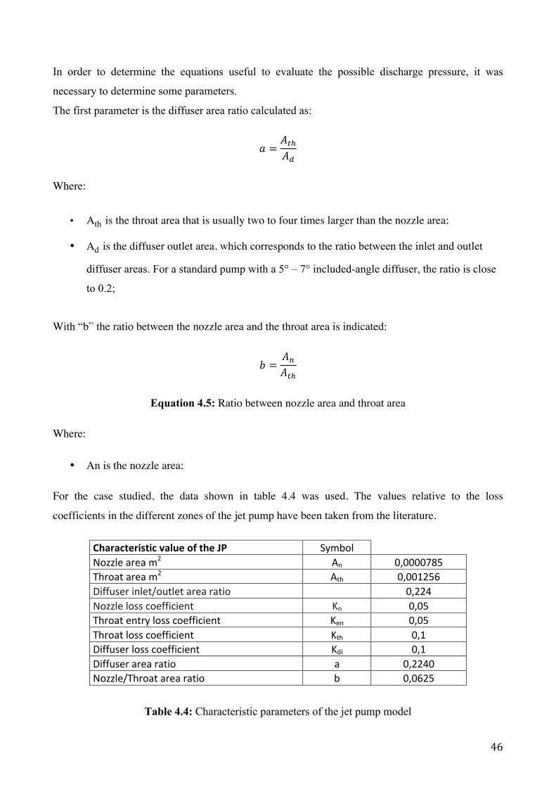
For the case studied, the data shown in table 4.4 was used. The values relative to the loss

coefficients in the different zones of the jet pump have been taken from the literature.

CharacteristicvalueoftheJP SymbolNozzleaream2 An 0,0000785

Throataream2 Ath 0,001256Diffuserinlet/outletarearatio 0,224Nozzlelosscoefficient Kn 0,05Throatentrylosscoefficient Ken 0,05Throatlosscoefficient Kth 0,1Diffuserlosscoefficient Kdi 0,1Diffuserarearatio a 0,2240Nozzle/Throatarearatio b 0,0625

Table 4.4: Characteristic parameters of the jet pump model

47

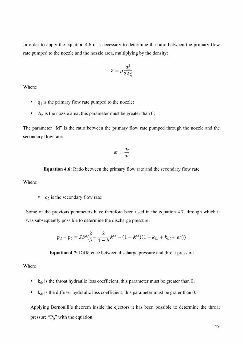
In order to apply the equation 4.6 it is necessary to determine the ratio between the primary flow

rate pumped to the nozzle and the nozzle area, multiplying by the density:

𝑍 = 𝜌𝑞!!

2𝐴!!

Where:

• q1 is the primary flow rate pumped to the nozzle;

• An is the nozzle area, this parameter must be greater than 0;

The parameter “M” is the ratio between the primary flow rate pumped through the nozzle and the

secondary flow rate:

𝑀 =𝑞!𝑞!

Equation 4.6: Ratio between the primary flow rate and the secondary flow rate

Where:

• q2 is the secondary flow rate;

Some of the previous parameters have therefore been used in the equation 4.7, through which it

was subsequently possible to determine the discharge pressure.

𝑝! − 𝑝! = 𝑍𝑏!(2𝑏 +

21− 𝑏𝑀

! − 1−𝑀! 1+ 𝑘!! + 𝑘!" + 𝑎! )

Equation 4.7: Difference between discharge pressure and throat pressure

Where

• kth is the throat hydraulic loss coefficient, this parameter must be greater than 0;

• kdi is the diffuser hydraulic loss coefficient, this parameter must be grater than 0;

Applying Bernoulli’s theorem inside the ejectors it has been possible to determine the throat

pressure “P0” with the equation:

48

𝑃! = 𝑃! +12 𝑣!

!𝜌 + 𝑃! +12 𝑣!

!𝜌 − ∆𝑃 − (12 𝑣!!

! 𝜌)

Equation 4.8: Bernoulli’s theorem to determine throat pressure

In the equation 4.8 the value of ΔP corresponds to the pressure losses in the nozzle area. After

calculating the throat pressure it is easy to find the discharge pressure by reversing the equation

4.9 obtaining the following equation:

𝑝! = 𝑍𝑏!2𝑏 +

21− 𝑏𝑀

! − 1−𝑀! 1+ 𝑘!! + 𝑘!" + 𝑎! + 𝑝!

Equation 4.9: Discharge pressure

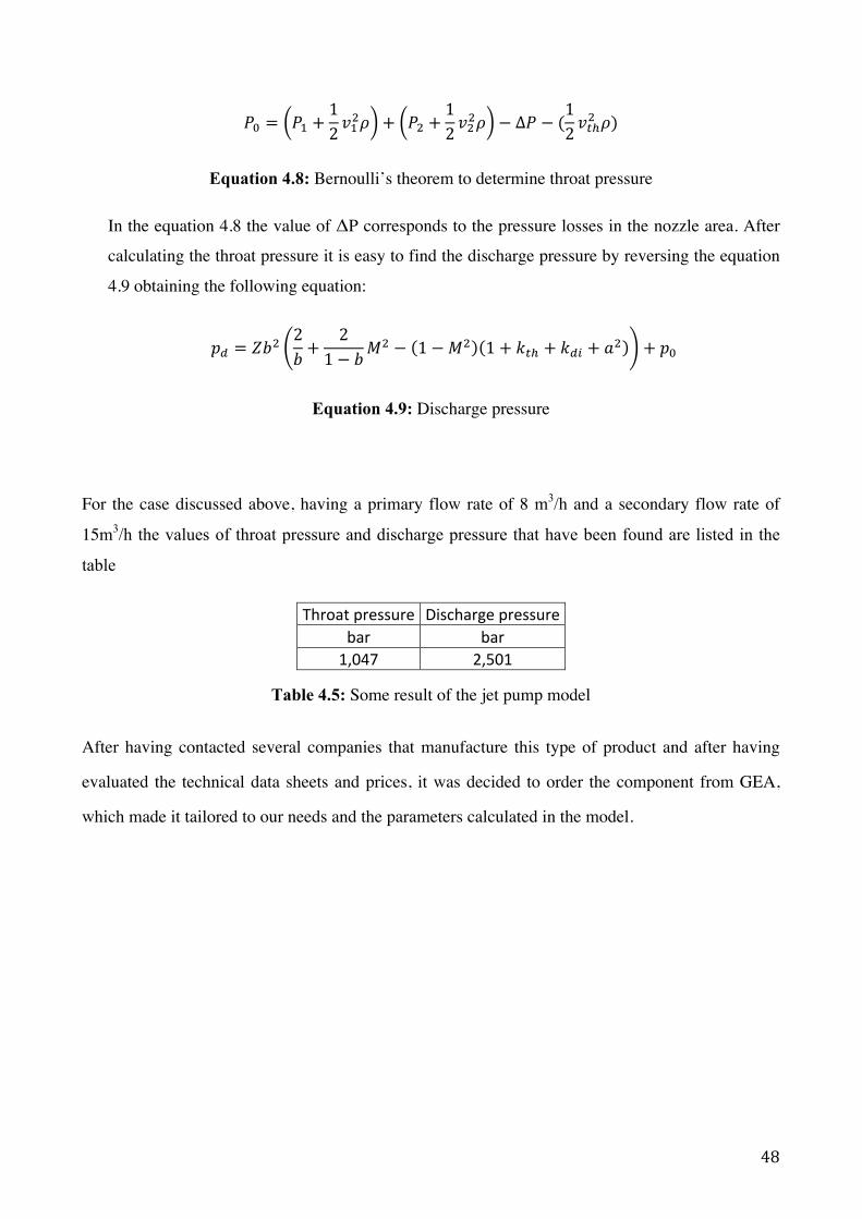
For the case discussed above, having a primary flow rate of 8 m3/h and a secondary flow rate of

15m3/h the values of throat pressure and discharge pressure that have been found are listed in the

table

Throatpressure Dischargepressurebar bar1,047 2,501

Table 4.5: Some result of the jet pump model

After having contacted several companies that manufacture this type of product and after having

evaluated the technical data sheets and prices, it was decided to order the component from GEA,

which made it tailored to our needs and the parameters calculated in the model.

49

4.6Sensor

In order to measure the pressure and the flow rate, different types of sensors have been installed on

the new configuration of the flushing rig under study.

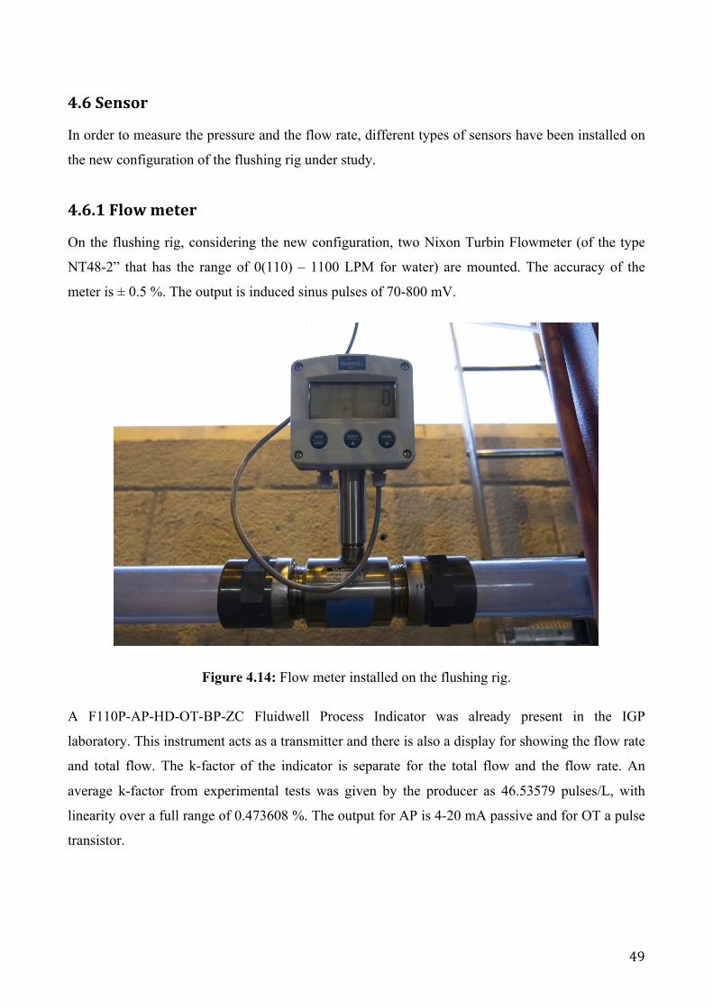
4.6.1Flowmeter

On the flushing rig, considering the new configuration, two Nixon Turbin Flowmeter (of the type

NT48-2” that has the range of 0(110) – 1100 LPM for water) are mounted. The accuracy of the

meter is ± 0.5 %. The output is induced sinus pulses of 70-800 mV.

Figure 4.14: Flow meter installed on the flushing rig.

A F110P-AP-HD-OT-BP-ZC Fluidwell Process Indicator was already present in the IGP

laboratory. This instrument acts as a transmitter and there is also a display for showing the flow rate

and total flow. The k-factor of the indicator is separate for the total flow and the flow rate. An

average k-factor from experimental tests was given by the producer as 46.53579 pulses/L, with

linearity over a full range of 0.473608 %. The output for AP is 4-20 mA passive and for OT a pulse

transistor.

50

4.6.2Pressuresensor

In the new configuration, three pressure sensors have been positioned. The first pressure sensor is

located in the upper left side of the U-shaped jumper, precisely at the height of the first elbow,

instead the other two pressure sensors are positioned respectively before and after the jet pump. The

type is from the UNIK 5000 pressure-sensing platform, more precisely the PTX 5072-tc-al-ca-h1-

pa. This is a resistive pressure transducer where an output signal of 4-20 mA is proportional to the

pressure applied. According to General Electric Company (2014) the sensors are a good solution for

reliable, accurate and economical measurements in a long term. More detailed information about

the pressure sensor located in the flushing rig can be found in the Appendix C.

51

4.7Methodtodeterminethevolumefractioninsidethepipes

In the previous work by Folde (2017), in order to calculate the volume fraction of the liquids

present in the jumper, the system was drained into 15 L transparent buckets that has a measurement

scale from 1 to 12 L, with steps of 0.1 L. The measurement readings uncertainty has been estimated

in ± 0.1 L. The transparency made it simple to distinguish between red colour Exxsol D60 and tap

water and, as a consequence, it was possible to determine the volume fraction.

Considering the new configuration, it would probably have been more complex to drain the liquid

in a bucket and, consequently, this could have led to more uncertainty in the final result. It was

therefore useful to find a new method to determine the volume fraction inside the pipes.

Starting from the assumption that both the total volume of the jumper and the diameter are known

(as a consequence also the radius), a ruler has been glued on each horizontal tube of the jumper in

order to determine the level of the oil-water interface as it is possible to observe in figure 4.15.

Figure 4.15: Meter placed on the pipe for the determination of the volume fraction.

During the experiments, several photos were taken at different time steps at all the meters located in

different parts of the jumper so as to be able to determine subsequently the parameter "S" which is,

as it is possible to see in figure 4.16, simply the measure of the oil height with respect to the height

of water, read on the meter placed on the pipes.

After determining the parameter “S”, already knowing the dimension of the radius "r", it is easy to

52

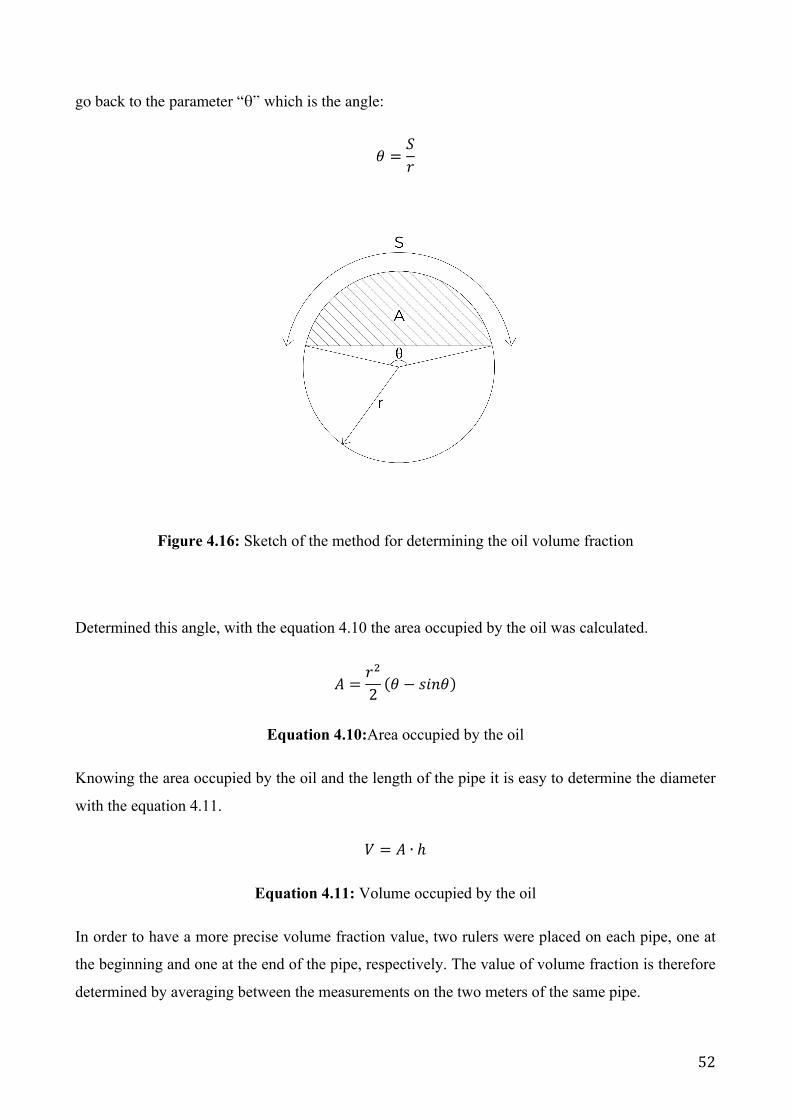
go back to the parameter “θ” which is the angle:

𝜃 =𝑆𝑟

Figure 4.16: Sketch of the method for determining the oil volume fraction

Determined this angle, with the equation 4.10 the area occupied by the oil was calculated.

𝐴 =𝑟!

2 𝜃 − 𝑠𝑖𝑛𝜃

Equation 4.10:Area occupied by the oil

Knowing the area occupied by the oil and the length of the pipe it is easy to determine the diameter

with the equation 4.11.

𝑉 = 𝐴 ∙ ℎ

Equation 4.11: Volume occupied by the oil

In order to have a more precise volume fraction value, two rulers were placed on each pipe, one at

the beginning and one at the end of the pipe, respectively. The value of volume fraction is therefore

determined by averaging between the measurements on the two meters of the same pipe.

53

As is well known, the U-shaped jumper is composed of both horizontal and vertical pipes.

However, the previous method cannot be used to determine the volume fraction for the vertical part

of the flushing rig as the two fluids have distinctly different densities and so they separate quickly

as shown in the figure 4.17. Reading the height of the oil in relation to the water using the previous

method would therefore not have given accurate results.

Figure 4.17:Oil column in the vertical part of the jumper.

Since the oil has a difference density with respect to water, the two phases eventually separate t and

it is therefore easy, knowing the characteristics dimensions of the pipes, to calculate the height of

the oil column in relation to the overall length of the pipe. Knowing the height of the pipe occupied

by the oil and the height of the pipe occupied by the water, it is therefore possible to calculate the

volume and consequently the volume fraction for the two fluids.

The total volume of the jumper is known, so adding the data collected from the analysis of all the

pipes, the total volume fraction was determined.

54

5.NumericalsimulationwithLedaFlow

Within this thesis work various simulations of what was then carried out in the laboratory were

performed. The simulations were performed with the LedaFlow simulator, taking into consideration

the different properties of the fluids, the characteristics of the tubes, the characteristic parameters of

the pumps and the environmental conditions present in the laboratory.

The simulations are executed to study different displacement rates, displacement times and

displacement fluids.

5.1GeneralcharacteristicsofthesimulationsinLedaFlowLedaFlow simulator allows realizing different system configurations, inserting also components like

pumps, valves, separator, and considering factors like leaks in pipes. For the case studied, two

different models were considered. The first model consist of only the U-shaped jumper, an inlet and

outlet node, instead the second model takes into account the presence of different pipes for the

recirculation of the fluids, a pump and a source.

These systems are used both to study the water that displaces oil and to study the oil that displaces

water. The tube is initially filled with the fluid to be displaced.

The fluids that are used for both simulations are tap water and oil Exxsol D60. This particularly

type of oil is produced from petroleum-based raw materials which are treated with hydrogen in the

presence of a catalyst to produce a low smell, low aromatic hydrocarbon solvent. The major

components include normal paraffin, isoparaffins, and cycloparaffins.

The main characteristics of the fluids that have been inserted to set the models are listed in the table

below.

Density Viscosity Compressibility Conductivity HeatCapacity Molarmass

kg/m^3 Pas Kg/m^3/bar W/m-K J/kg-K g/mol

Water 998,9 0,001095 0,0391 0,6069 4183,8 18,02Oil(ExxsolD60) 786 0,00156 0,0391 0,136 1760 158

Table 5.1: Principal characteristics of the fluid used for the simulations

LedaFlow also allows entering the parameters that characterize the material of which the U-jumper

and the others pipes are made, in this case PVC. The properties useful to set the models created in

LedaFlow are presented in the table 5.2.

55

Property Symbol ValueDensity ρPVC 1400Kg/m^3

Heatcapacity cp 1005J/Kg°CConductivity k 0,19W/(mK)Emissivity ε 0,92

Young’smodulus E 3,25GpaViscosity μPVC 0Pa-s

Thermalexpansioncoefficient α 01/C

Table 5.2: Characteristics parameter of the PVC pipes

5.2GeometryandcharacteristicsofthefirstmodelAs described previously, the first model is built taking into account only the U-shaped jumper, an

inlet and outlet nodes. For the nodes placed at the beginning and at the end of the jumper,

temperature and pressure conditions were chosen over time. In the inlet node it is also possible to

set the flow rate, expressed in kg/s.

Figure 5.1: Network of the U-shaped jumper in LedaFlow

In the pipe settings are the profile and geometry of the pipe, as well as the mesh constructed. The

profile is created in a Cartesian coordinate system, in two dimensional, using X and Z. The

measures are initially based on the thesis of Opstvedt (2016) with some adjustments made by Folde

(2017) to fit the measured drainable volume of 165.98 L.

However, according to the experiment conducted by Folde (2017), it should be noticed that after all

of the experiments conducted, the average measured total volume was 165.0 L ± 0.3 L.

In order to make a more accurate model, the variation in diameter in the elbows has been taken into

account, as it is possible to observe from the table 5.4. The characteristic dimensions of the jumper

are shown in the table 5.3.

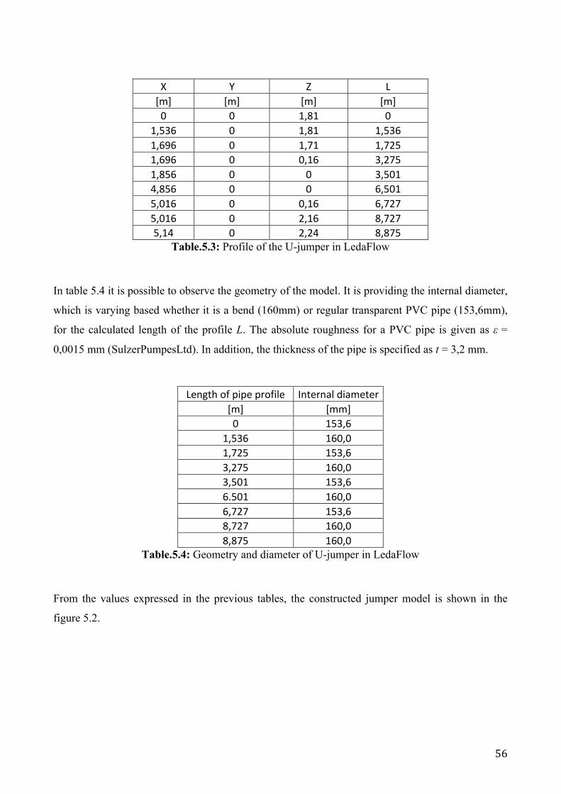
56

X Y Z L[m] [m] [m] [m]0 0 1,81 0

1,536 0 1,81 1,5361,696 0 1,71 1,7251,696 0 0,16 3,2751,856 0 0 3,5014,856 0 0 6,5015,016 0 0,16 6,7275,016 0 2,16 8,7275,14 0 2,24 8,875

Table.5.3: Profile of the U-jumper in LedaFlow

In table 5.4 it is possible to observe the geometry of the model. It is providing the internal diameter,

which is varying based whether it is a bend (160mm) or regular transparent PVC pipe (153,6mm),

for the calculated length of the profile L. The absolute roughness for a PVC pipe is given as ε =

0,0015 mm (SulzerPumpesLtd). In addition, the thickness of the pipe is specified as t = 3,2 mm.

Lengthofpipeprofile Internaldiameter

[m] [mm]0 153,6

1,536 160,01,725 153,63,275 160,03,501 153,66.501 160,06,727 153,68,727 160,08,875 160,0

Table.5.4: Geometry and diameter of U-jumper in LedaFlowFrom the values expressed in the previous tables, the constructed jumper model is shown in the

figure 5.2.

57

Figure 5.2: U-jumper constructed by Leda Flow simulator.

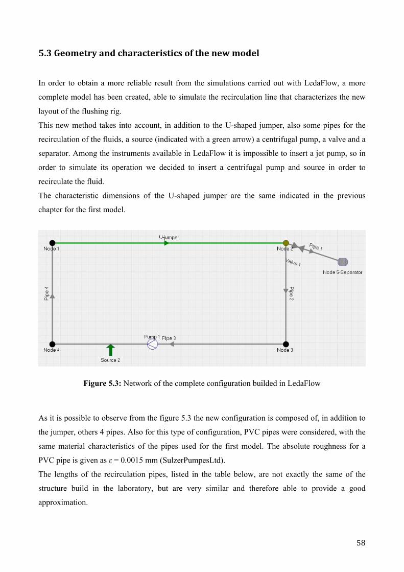
58

5.3Geometryandcharacteristicsofthenewmodel

In order to obtain a more reliable result from the simulations carried out with LedaFlow, a more

complete model has been created, able to simulate the recirculation line that characterizes the new

layout of the flushing rig.

This new method takes into account, in addition to the U-shaped jumper, also some pipes for the

recirculation of the fluids, a source (indicated with a green arrow) a centrifugal pump, a valve and a

separator. Among the instruments available in LedaFlow it is impossible to insert a jet pump, so in

order to simulate its operation we decided to insert a centrifugal pump and source in order to

recirculate the fluid.

The characteristic dimensions of the U-shaped jumper are the same indicated in the previous

chapter for the first model.

Figure 5.3: Network of the complete configuration builded in LedaFlow

As it is possible to observe from the figure 5.3 the new configuration is composed of, in addition to

the jumper, others 4 pipes. Also for this type of configuration, PVC pipes were considered, with the

same material characteristics of the pipes used for the first model. The absolute roughness for a

PVC pipe is given as ε = 0.0015 mm (SulzerPumpesLtd).

The lengths of the recirculation pipes, listed in the table below, are not exactly the same of the

structure build in the laboratory, but are very similar and therefore able to provide a good

approximation.

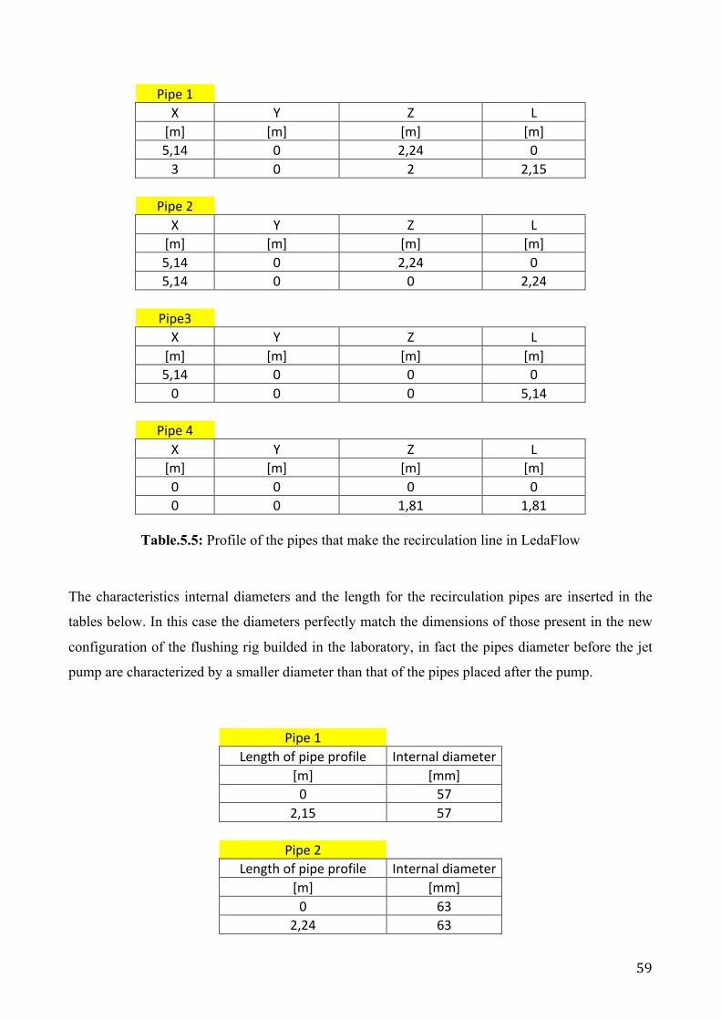
59

Pipe1 X Y Z L

[m] [m] [m] [m]5,14 0 2,24 03 0 2 2,15

Pipe2 X Y Z L

[m] [m] [m] [m]5,14 0 2,24 05,14 0 0 2,24

Pipe3 X Y Z L

[m] [m] [m] [m]5,14 0 0 00 0 0 5,14

Pipe4 X Y Z L

[m] [m] [m] [m]0 0 0 00 0 1,81 1,81

Table.5.5: Profile of the pipes that make the recirculation line in LedaFlow

The characteristics internal diameters and the length for the recirculation pipes are inserted in the

tables below. In this case the diameters perfectly match the dimensions of those present in the new

configuration of the flushing rig builded in the laboratory, in fact the pipes diameter before the jet

pump are characterized by a smaller diameter than that of the pipes placed after the pump.

Pipe1Lengthofpipeprofile Internaldiameter

[m] [mm]0 57

2,15 57


[m] [mm]0 63

2,24 63

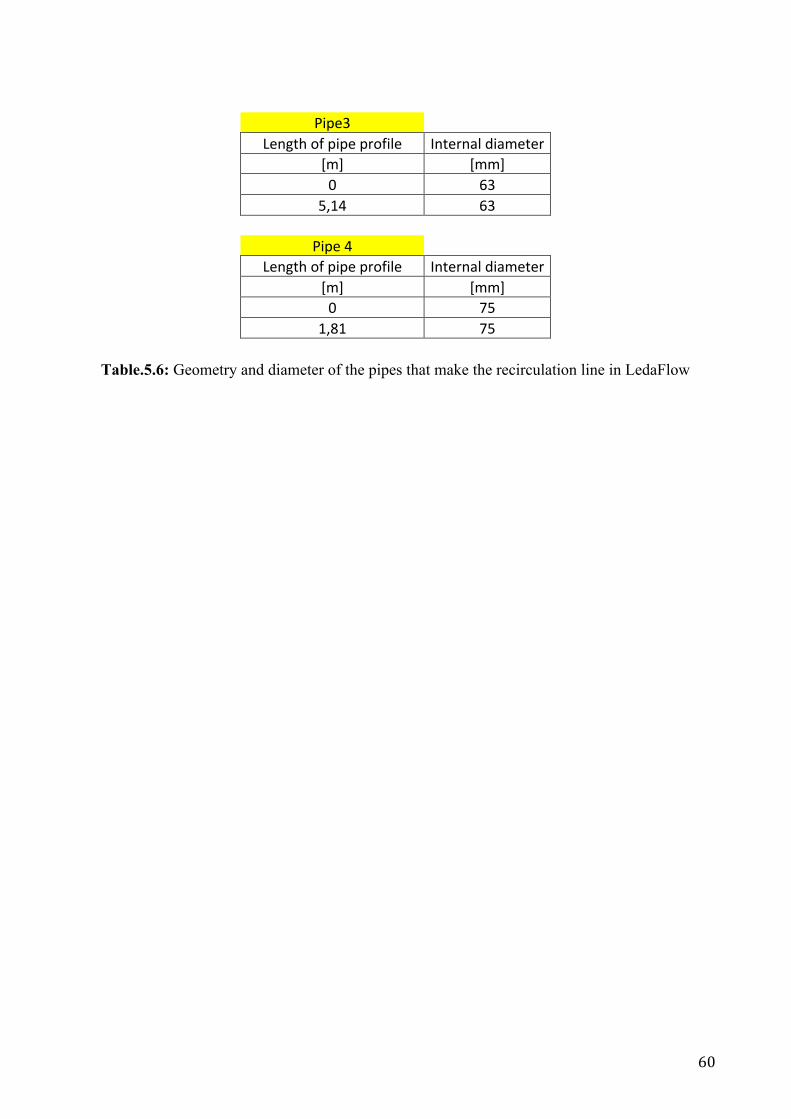
60


[m] [mm]0 63

5,14 63


[m] [mm]0 75

1,81 75

Table.5.6: Geometry and diameter of the pipes that make the recirculation line in LedaFlow

61

5.4LabViewLabVIEW (Laboratory Virtual Instrumentation Engineering Workbench) is the integrated

development environment for the National Instruments visual programming language. With the aim

of recording the measured values from all the three pressure sensors and the two flow meters

described in the previous chapter, the LabView software was used. The block diagram for the

studied case is visualized in Figure 5.4.

Figure 5.4: Virtual instrumentation block diagram with LabView

62

6.ResultsIn this chapter the results obtained through the mathematical model and the simulations that have

been realized with LedaFlow are presented. Additionally, a comparison between all the results of

the experiments carried out in the laboratory is given; unfortunately, there is not a huge amount of

values due to time constraints that did not allowed to reproduce many experiments in the laboratory.

It was therefore decided to reproduce only the cases in which water displace oil with three different

injected flow rates.

6.1LedaFlowsimulationwithsimpleconfigurationConsidering the model created with LedaFlow is made up only of the jumper, simulations were

performed both for the case in which water displacing oil and for oil displacing water, starting from

different injected flow rate. The results are shown in this chapter. 6.1.1OildisplacingwaterThe results from the LedaFlow simulation where oil is displacing water are displayed in Table 6.1.

As you can see from the table below, four different simulations have been conducted, characterized

by a different injected flow rate. The boundary conditions (geometry of the jumper and

characteristic parameters of the fluids are the same) remain unchanged.

5m^3/h 8m^3/h 12m^3/h 20,77m^3/h

Time WaterVFLedaFlow WaterVFLedaFlow WaterVFLedaFlow WaterVFLedaFlow[s] [-] [-] [-] [-]0 1 1 1 120 0,8036 0,6925 0,5365 0,231240 0,6135 0,3905 0,2279 0,055060 0,4322 0,2733 0,1574 0,032480 0,3648 0,2380 0,1360 0,027280 0,3648 0,2380 0,1360 0,0272100 0,3448 0,2280 0,1340 0,0272120 0,3391 0,2170 0,1302 0,0255140 0,3371 0,2133 0,1302 0,0254180 0,3363 0,2101 0,1300 0,0253220 0,3360 0,2061 0,1300 0,0252260 0,3358 0,2069 0,1300 0,0252300 0,3357 0,2068 0,1300 0,0252400 0,3355 0,2060 0,1300 0,0252

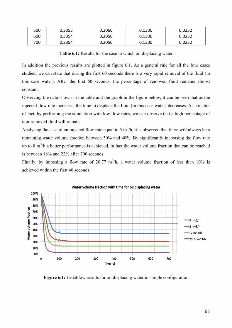
63

500 0,3355 0,2060 0,1300 0,0252600 0,3354 0,2050 0,1300 0,0252700 0,3354 0,2050 0,1300 0,0252

Table 6.1: Results for the case in which oil displacing water

In addition the previous results are plotted in figure 6.1. As a general rule for all the four cases

studied, we can state that during the first 60 seconds there is a very rapid removal of the fluid (in

this case water). After the first 60 seconds, the percentage of removed fluid remains almost

constant.

Observing the data shown in the table and the graph in the figure below, it can be seen that as the

injected flow rate increases, the time to displace the fluid (in this case water) decreases. As a matter

of fact, by performing the simulation with low flow rates, we can observe that a high percentage of

non-removed fluid will remain.

Analysing the case of an injected flow rate equal to 5 m3/h, it is observed that there will always be a

remaining water volume fraction between 30% and 40%. By significantly increasing the flow rate

up to 8 m3/h a better performance is achieved, in fact the water volume fraction that can be reached

is between 18% and 22% after 700 seconds.

Finally, by imposing a flow rate of 20.77 m3/h, a water volume fraction of less than 10% is

achieved within the first 40 seconds.

Figure 6.1: LedaFlow results for oil displacing water in simple configuration

64

6.1.2WaterdisplacingoilThe results from water displacing oil are presented in Figure 6.2 and Table 6.2. The graph and the

table are presenting the oil volume fractions as a function of time for four different flow rates which

are the same simulated for the previous case in which oil displacing water.

5m^3/h 8m^3/h 12m^3/h 20,769m^3/h

Time OilVFLedaFlow OilVFLedaFlow OilVFLedaFlow OilVFLedaFlow[s] [-] [-] [-] [-]0 1 1 1 120 0,8531 0,7629 0,6400 0,399840 0,7098 0,5251 0,2878 0,144960 0,5602 0,2891 0,1894 0,094680 0,4122 0,2170 0,1518 0,0731100 0,2791 0,2058 0,1398 0,0662120 0,2735 0,2014 0,1345 0,0629140 0,2710 0,1989 0,1314 0,0605180 0,2682 0,1962 0,1279 0,0599220 0,2668 0,1944 0,1251 0,0599260 0,2657 0,1928 0,1233 0,0599300 0,2639 0,1914 0,1230 0,0599400 0,2619 0,1903 0,1230 0,0599500 0,2607 0,1902 0,1230 0,0599600 0,2603 0,1902 0,1230 0,0599700 0,2602 0,1902 0,1230 0,0599

Table 6.2: Results for the case in which water displacing oil

Observing the chart also in this case we can state that, as a general rule, for all the four cases it can

be seen that during the first 100 seconds we have a very rapid removal of the fluid (in this case oil).

After the first 100 seconds the percentage of removed fluid remains almost constant.

Indeed, it is possible to state that increasing the injected flow rate, the time to displace the fluid (in

this case oil) decreases.

It should be noticed that it seems like the displacement ability for a water flow rate to displace the

oil in the system is higher than the one for an oil rate displacing water in the system. This might be

due to differences in flow rate, density or viscosities.

From the processed data and the chart in figure 6.1 and 6.2 it is possible to see that, with this type of

configuration, imposing lower flow rates the efficiency is higher in the case of water that displacing

oil. It is possible to observe that, imposing a flow rate of 5 m3/h at 700 seconds we will have a water

65

oil volume fraction less than 30%. In the case in which water displacing oil, imposing the same

flow rate at 700 seconds, it is observed a water volume fraction between 32% and 35%.

On the contrary, instead, as can be seen from the data collected in the tables 6.1 and 6.2, if the

maximum flow rate of 20.77 m3/h is imposed, the efficiency is higher in case in which oil

displacing water.

Figure 6.2: LedaFlow results for water displacing oil in simple configuration

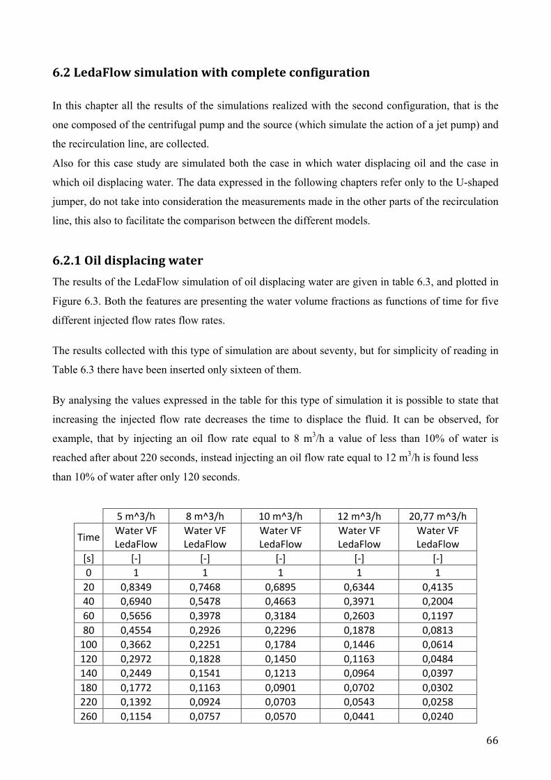
66

6.2LedaFlowsimulationwithcompleteconfiguration

In this chapter all the results of the simulations realized with the second configuration, that is the

one composed of the centrifugal pump and the source (which simulate the action of a jet pump) and

the recirculation line, are collected.

Also for this case study are simulated both the case in which water displacing oil and the case in

which oil displacing water. The data expressed in the following chapters refer only to the U-shaped

jumper, do not take into consideration the measurements made in the other parts of the recirculation

line, this also to facilitate the comparison between the different models.

6.2.1OildisplacingwaterThe results of the LedaFlow simulation of oil displacing water are given in table 6.3, and plotted in

Figure 6.3. Both the features are presenting the water volume fractions as functions of time for five

different injected flow rates flow rates.

The results collected with this type of simulation are about seventy, but for simplicity of reading in

Table 6.3 there have been inserted only sixteen of them.

By analysing the values expressed in the table for this type of simulation it is possible to state that

increasing the injected flow rate decreases the time to displace the fluid. It can be observed, for

example, that by injecting an oil flow rate equal to 8 m3/h a value of less than 10% of water is

reached after about 220 seconds, instead injecting an oil flow rate equal to 12 m3/h is found less

than 10% of water after only 120 seconds.

5m^3/h 8m^3/h 10m^3/h 12m^3/h 20,77m^3/h

Time WaterVFLedaFlow

WaterVFLedaFlow

WaterVFLedaFlow

WaterVFLedaFlow

WaterVFLedaFlow

[s] [-] [-] [-] [-] [-]0 1 1 1 1 120 0,8349 0,7468 0,6895 0,6344 0,413540 0,6940 0,5478 0,4663 0,3971 0,200460 0,5656 0,3978 0,3184 0,2603 0,119780 0,4554 0,2926 0,2296 0,1878 0,0813100 0,3662 0,2251 0,1784 0,1446 0,0614120 0,2972 0,1828 0,1450 0,1163 0,0484140 0,2449 0,1541 0,1213 0,0964 0,0397180 0,1772 0,1163 0,0901 0,0702 0,0302220 0,1392 0,0924 0,0703 0,0543 0,0258260 0,1154 0,0757 0,0570 0,0441 0,0240

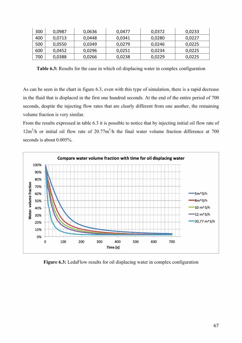
67

300 0,0987 0,0636 0,0477 0,0372 0,0233400 0,0713 0,0448 0,0341 0,0280 0,0227500 0,0550 0,0349 0,0279 0,0246 0,0225600 0,0452 0,0296 0,0251 0,0234 0,0225700 0,0388 0,0266 0,0238 0,0229 0,0225

Table 6.3: Results for the case in which oil displacing water in complex configuration

As can be seen in the chart in figure 6.3, even with this type of simulation, there is a rapid decrease

in the fluid that is displaced in the first one hundred seconds. At the end of the entire period of 700

seconds, despite the injecting flow rates that are clearly different from one another, the remaining

volume fraction is very similar.

From the results expressed in table 6.3 it is possible to notice that by injecting initial oil flow rate of

12m3/h or initial oil flow rate of 20.77m3/h the final water volume fraction difference at 700

seconds is about 0.005%.

Figure 6.3: LedaFlow results for oil displacing water in complex configuration

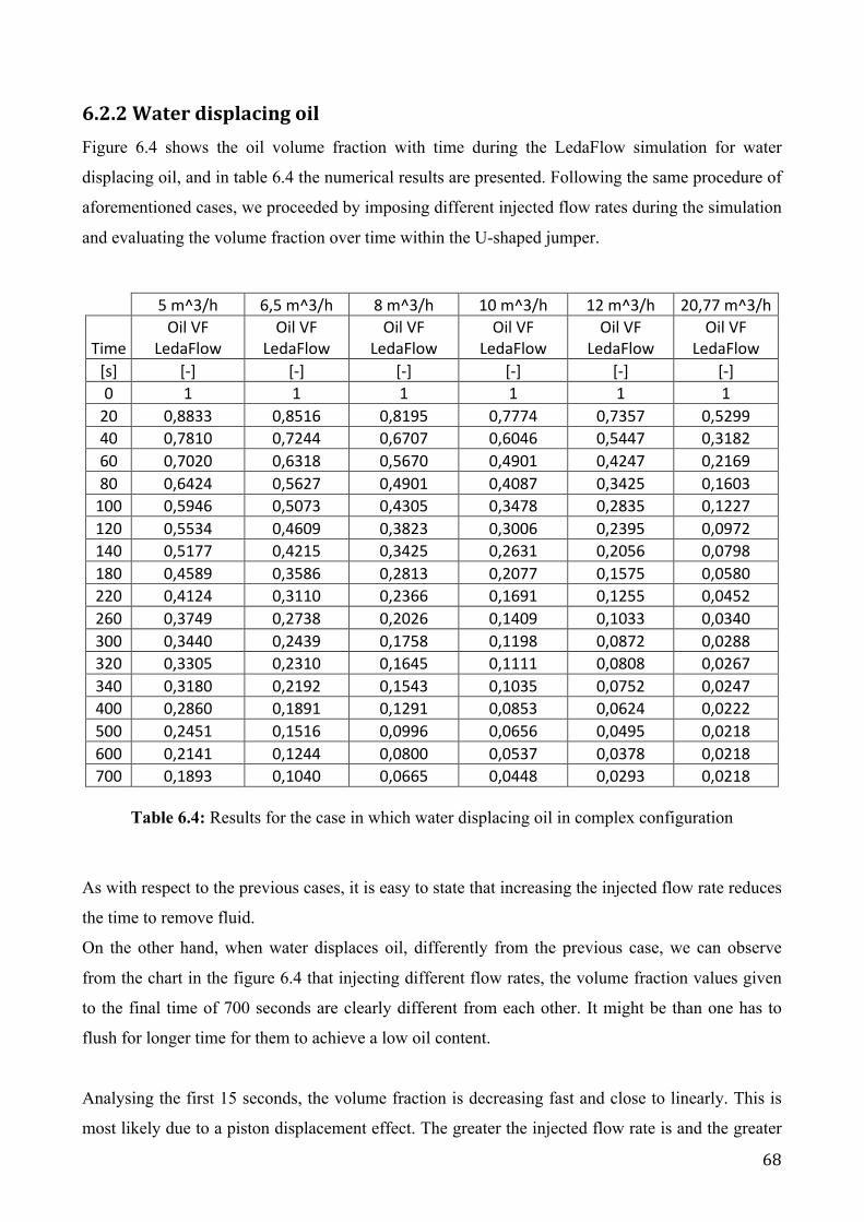
68

6.2.2WaterdisplacingoilFigure 6.4 shows the oil volume fraction with time during the LedaFlow simulation for water

displacing oil, and in table 6.4 the numerical results are presented. Following the same procedure of

aforementioned cases, we proceeded by imposing different injected flow rates during the simulation

and evaluating the volume fraction over time within the U-shaped jumper.

5m^3/h 6,5m^3/h 8m^3/h 10m^3/h 12m^3/h 20,77m^3/h

TimeOilVF

LedaFlowOilVF

LedaFlowOilVF

LedaFlowOilVF

LedaFlowOilVF

LedaFlowOilVF

LedaFlow[s] [-] [-] [-] [-] [-] [-]0 1 1 1 1 1 120 0,8833 0,8516 0,8195 0,7774 0,7357 0,529940 0,7810 0,7244 0,6707 0,6046 0,5447 0,318260 0,7020 0,6318 0,5670 0,4901 0,4247 0,216980 0,6424 0,5627 0,4901 0,4087 0,3425 0,1603100 0,5946 0,5073 0,4305 0,3478 0,2835 0,1227120 0,5534 0,4609 0,3823 0,3006 0,2395 0,0972140 0,5177 0,4215 0,3425 0,2631 0,2056 0,0798180 0,4589 0,3586 0,2813 0,2077 0,1575 0,0580220 0,4124 0,3110 0,2366 0,1691 0,1255 0,0452260 0,3749 0,2738 0,2026 0,1409 0,1033 0,0340300 0,3440 0,2439 0,1758 0,1198 0,0872 0,0288320 0,3305 0,2310 0,1645 0,1111 0,0808 0,0267340 0,3180 0,2192 0,1543 0,1035 0,0752 0,0247400 0,2860 0,1891 0,1291 0,0853 0,0624 0,0222500 0,2451 0,1516 0,0996 0,0656 0,0495 0,0218600 0,2141 0,1244 0,0800 0,0537 0,0378 0,0218700 0,1893 0,1040 0,0665 0,0448 0,0293 0,0218

Table 6.4: Results for the case in which water displacing oil in complex configuration

As with respect to the previous cases, it is easy to state that increasing the injected flow rate reduces

the time to remove fluid.

On the other hand, when water displaces oil, differently from the previous case, we can observe

from the chart in the figure 6.4 that injecting different flow rates, the volume fraction values given

to the final time of 700 seconds are clearly different from each other. It might be than one has to

flush for longer time for them to achieve a low oil content.

Analysing the first 15 seconds, the volume fraction is decreasing fast and close to linearly. This is

most likely due to a piston displacement effect. The greater the injected flow rate is and the greater

69

effect this volume will have on the oil volume fraction, in fact it is possible to observe that injecting

a flow rate of 20.77 m3/h this effect lasts up to an oil volume fraction of about 54%, instead

injecting a flow of 10 m3/h or 12 m^3/h the piston effect the oil volume fraction remain between

70% and 80%.

Figure 6.4: LedaFlow results for water displacing oil in complex configuration

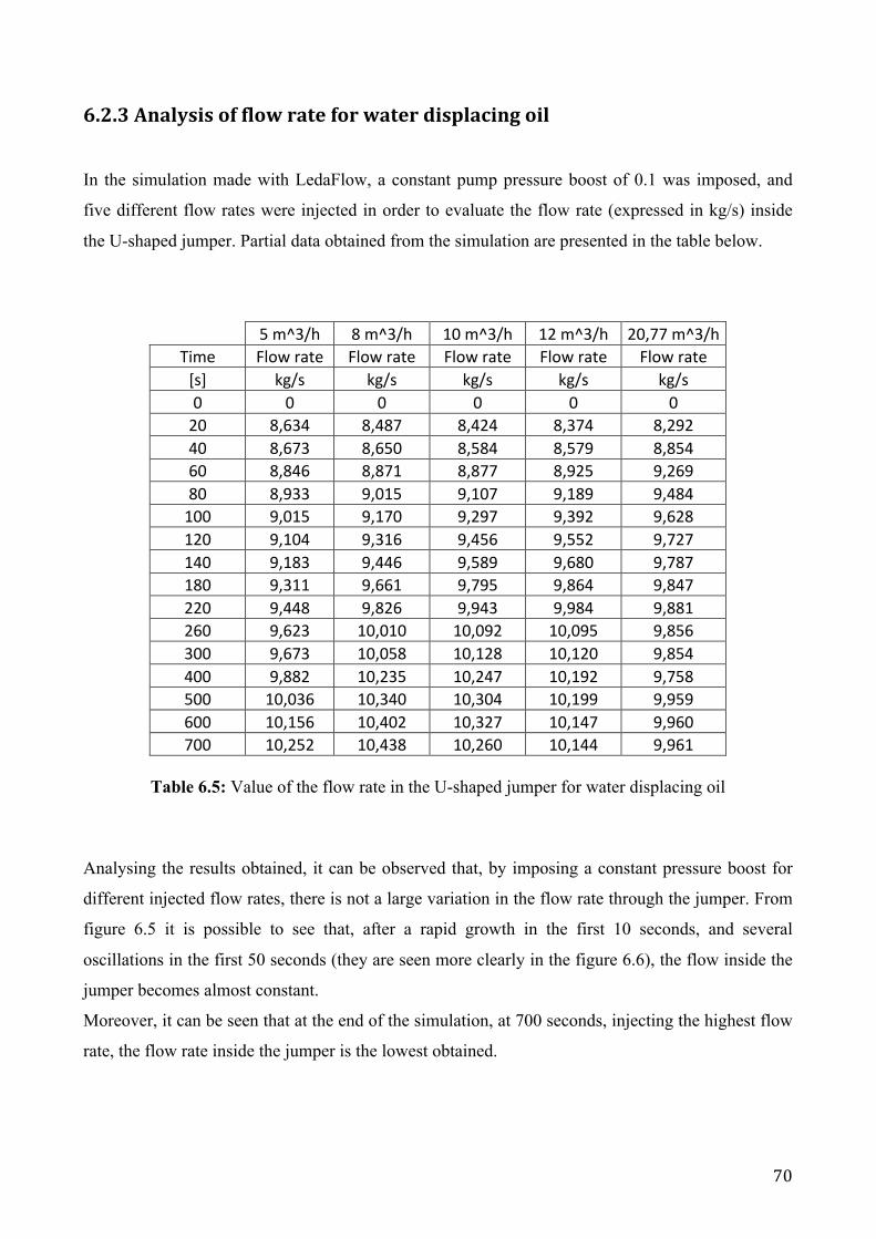
70

6.2.3Analysisofflowrateforwaterdisplacingoil

In the simulation made with LedaFlow, a constant pump pressure boost of 0.1 was imposed, and

five different flow rates were injected in order to evaluate the flow rate (expressed in kg/s) inside

the U-shaped jumper. Partial data obtained from the simulation are presented in the table below.

5m^3/h 8m^3/h 10m^3/h 12m^3/h 20,77m^3/h

Time Flowrate Flowrate Flowrate Flowrate Flowrate[s] kg/s kg/s kg/s kg/s kg/s0 0 0 0 0 020 8,634 8,487 8,424 8,374 8,29240 8,673 8,650 8,584 8,579 8,85460 8,846 8,871 8,877 8,925 9,26980 8,933 9,015 9,107 9,189 9,484100 9,015 9,170 9,297 9,392 9,628120 9,104 9,316 9,456 9,552 9,727140 9,183 9,446 9,589 9,680 9,787180 9,311 9,661 9,795 9,864 9,847220 9,448 9,826 9,943 9,984 9,881260 9,623 10,010 10,092 10,095 9,856300 9,673 10,058 10,128 10,120 9,854400 9,882 10,235 10,247 10,192 9,758500 10,036 10,340 10,304 10,199 9,959600 10,156 10,402 10,327 10,147 9,960700 10,252 10,438 10,260 10,144 9,961

Table 6.5: Value of the flow rate in the U-shaped jumper for water displacing oil

Analysing the results obtained, it can be observed that, by imposing a constant pressure boost for

different injected flow rates, there is not a large variation in the flow rate through the jumper. From

figure 6.5 it is possible to see that, after a rapid growth in the first 10 seconds, and several

oscillations in the first 50 seconds (they are seen more clearly in the figure 6.6), the flow inside the

jumper becomes almost constant.

Moreover, it can be seen that at the end of the simulation, at 700 seconds, injecting the highest flow

rate, the flow rate inside the jumper is the lowest obtained.

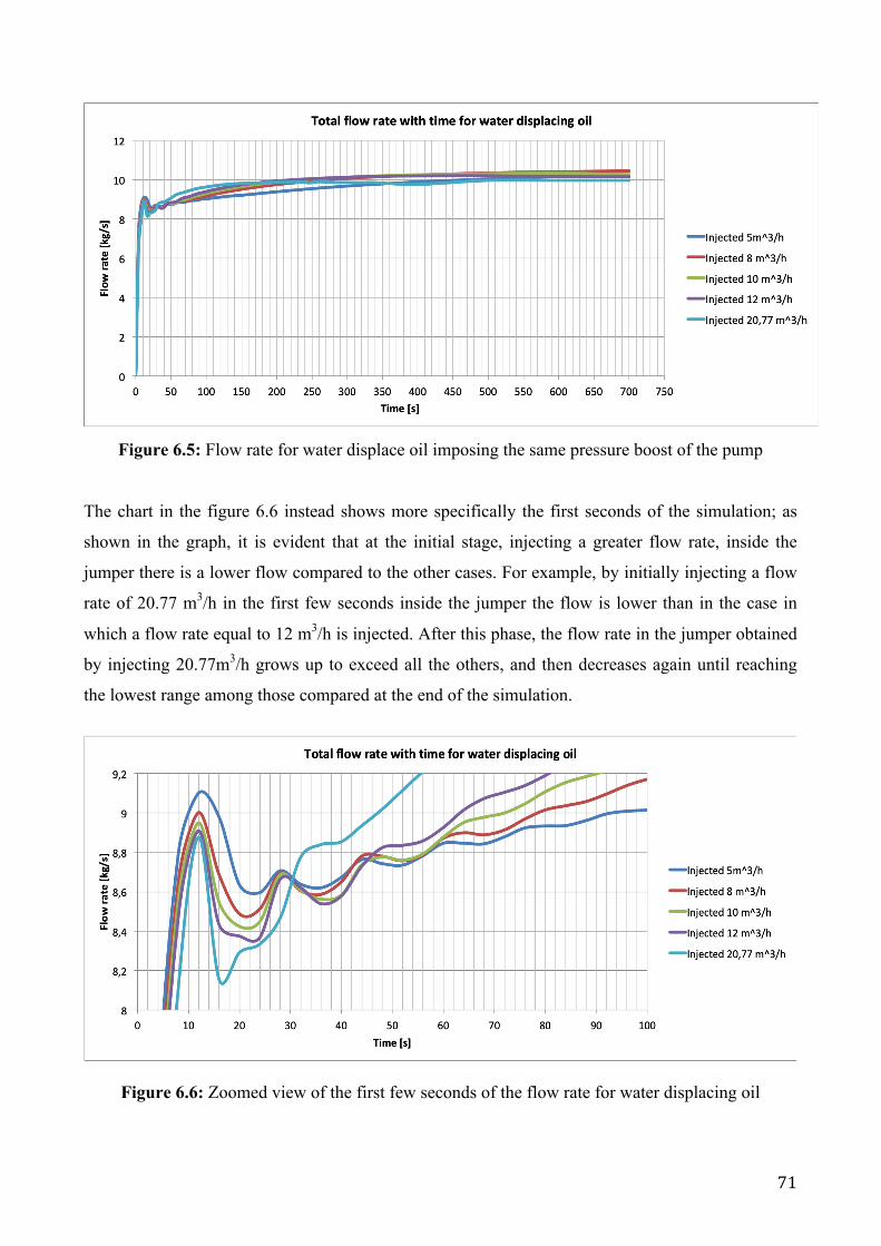
71

Figure 6.5: Flow rate for water displace oil imposing the same pressure boost of the pump

The chart in the figure 6.6 instead shows more specifically the first seconds of the simulation; as

shown in the graph, it is evident that at the initial stage, injecting a greater flow rate, inside the

jumper there is a lower flow compared to the other cases. For example, by initially injecting a flow

rate of 20.77 m3/h in the first few seconds inside the jumper the flow is lower than in the case in

which a flow rate equal to 12 m3/h is injected. After this phase, the flow rate in the jumper obtained

by injecting 20.77m3/h grows up to exceed all the others, and then decreases again until reaching

the lowest range among those compared at the end of the simulation.

Figure 6.6: Zoomed view of the first few seconds of the flow rate for water displacing oil

72

6.2.4 Analysis of the effect of the imposed pressure boost for waterdisplacingoilIt can be interesting to observe the behaviour of the oil volume fraction (always for the case in

which water displacing oil) imposing a constant injected flow rate but varying the pressure boost of

the centrifugal pump inserted in the model in LedaFlow.

In the case studied below, a constant flow rate of 12 m3/h was set and the pump pressure boost was

varied, taking into consideration values between 0.1 and 0.7 bar. During the simulations it was also

tried to further reduce the pressure boost below the minimum value of 0.1 bar, but by injecting the

fluid from the source, the latter ran the pipes in reverse direction because the pump was not able to

convey it in the right direction. The minimum value of 0.1 bar was chosen precisely because it is

the lowest value useful to make the fluid flow correctly in the flushing rig.

Figure 6.7: Oil volume fraction with time changing the pressure boost

As can be seen from the chart in figure 6.7 and from figure 6.8, which represent a detailed view of

the first graph, the trend of the oil volume fraction imposing different values of pressure boost is

very similar in all four simulated cases.

Watching closely at the chart in figure 6.8 we can state that, at the end of the time taken for the

simulation (always 700 seconds), a higher-pressure boost will give better results in terms of oil

volume fraction value in the jumper. In fact it is possible to observe that with a pressure boost of 0.7

there is a lower value of oil volume fraction.

By changing the pressure boost and leaving the injected flow rate constant, there are no major

advantages in terms of oil removed from the water, at least for the case in which water displacing

oil.

73

Figure 6.8: Details view for the chart in figure 6.7

Keeping the initial assumptions unchanged, a flow rate analysis within the jumper was also

conducted. It is possible to conclude that by keeping the injection flow rate constant and increasing

the pump pressure boost the flow rate inside the jumper also increases.

12m^3/hwith0,1bara

12m^3/hwith0,2bara

12m^3/hwith0,5bara

12m^3/hwith0,7bara

Time Flowrate Flowrate Flowrate Flowrate[s] kg/s kg/s kg/s kg/s0 0 0 0 020 8,3745 13,1859 22,5805 27,504940 8,5786 13,6265 23,5914 28,724360 8,9255 13,9550 24,1660 29,441080 9,1892 14,2456 24,6043 29,9820100 9,3923 14,4593 24,9669 30,4294120 9,5522 14,6417 25,2625 30,7948140 9,6799 14,7875 25,5048 31,0957180 9,8636 15,0067 25,8683 31,5469220 9,9840 15,1540 26,1135 31,8504260 10,0654 15,2539 26,2789 32,0543300 10,1204 15,3222 26,3898 32,1911400 10,1920 15,4090 26,5271 32,3608500 10,1987 15,4330 26,5636 32,4071600 10,1472 15,3239 26,4025 32,2224700 10,1440 15,2756 26,3147 32,1215

Table 6.6: Value of the flow rate in the jumper for water displacing oil changing pressure boost

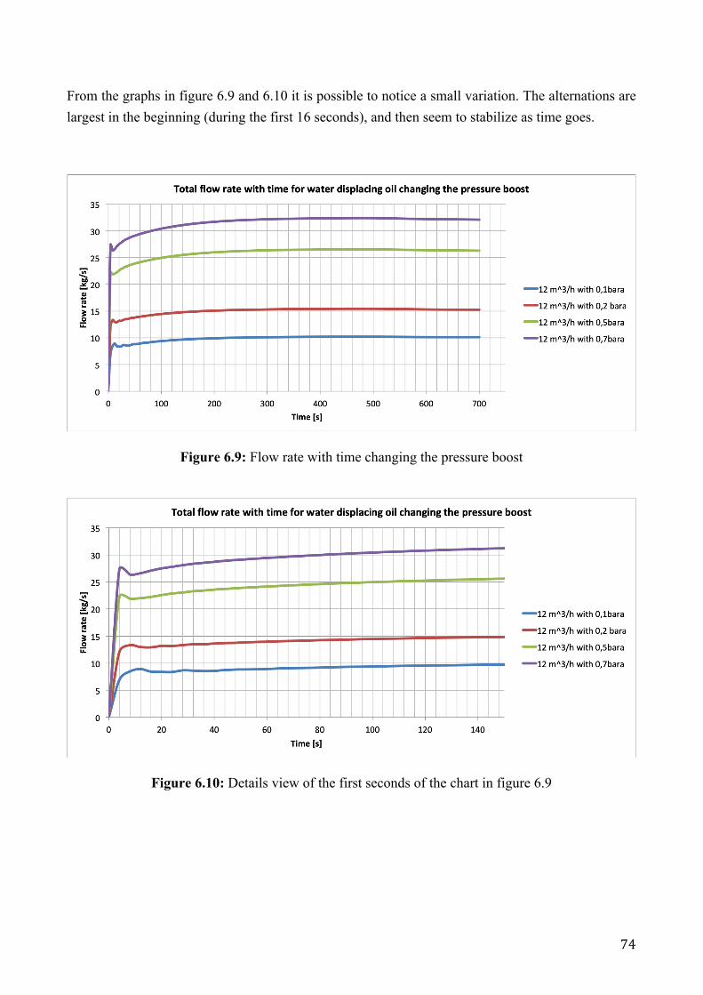
74

From the graphs in figure 6.9 and 6.10 it is possible to notice a small variation. The alternations are largest in the beginning (during the first 16 seconds), and then seem to stabilize as time goes.

Figure 6.9: Flow rate with time changing the pressure boost

Figure 6.10: Details view of the first seconds of the chart in figure 6.9

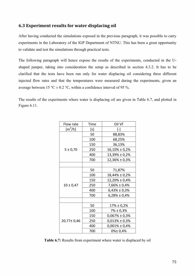
75

6.3ExperimentresultsforwaterdisplacingoilAfter having conducted the simulations exposed in the previous paragraph, it was possible to carry

experiments in the Laboratory of the IGP Department of NTNU. This has been a great opportunity

to validate and test the simulations through practical tests.

The following paragraph will hence expose the results of the experiments, conducted in the U-

shaped jumper, taking into consideration the setup as described in section 4.3.2. It has to be

clarified that the tests have been run only for water displacing oil considering three different

injected flow rates and that the temperatures were measured during the experiments, given an

average between 15 °C ± 0.2 °C, within a confidence interval of 95 %.

The results of the experiments where water is displacing oil are given in Table 6.7, and plotted in Figure 6.11.

Flowrate Time OilVF[m3/h] [s] [-]

50 88,83% 100 68,25% 150 36,13%5±0,70 250 16,10%±0,2%

400 13,39%±0,2% 700 12,36%±0,3% 50 71,87% 100 18,44%±0,2% 150 12,20%±0,4%10±0,47 250 7,66%±0,4%

400 6,43%±0,3% 700 6,28%±0,4% 50 17%±0,2% 100 7%±0,3% 150 0,067%±0,3%20,77±0,46 250 0,013%±0,3% 400 0,001%±0,4% 700 0%±0,4%

Table 6.7: Results from experiment where water is displaced by oil

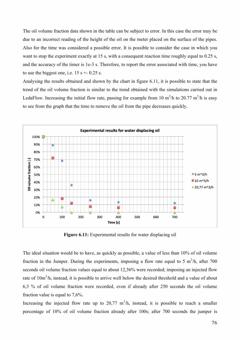
76

The oil volume fraction data shown in the table can be subject to error. In this case the error may be

due to an incorrect reading of the height of the oil on the meter placed on the surface of the pipes.

Also for the time was considered a possible error. It is possible to consider the case in which you

want to stop the experiment exactly at 15 s, with a consequent reaction time roughly equal to 0.25 s,

and the accuracy of the timer is 1e-3 s. Therefore, to report the error associated with time, you have

to use the biggest one, i.e. 15 s +- 0.25 s.

Analysing the results obtained and shown by the chart in figure 6.11, it is possible to state that the

trend of the oil volume fraction is similar to the trend obtained with the simulations carried out in

LedaFlow. Increasing the initial flow rate, passing for example from 10 m3/h to 20.77 m3/h is easy

to see from the graph that the time to remove the oil from the pipe decreases quickly.

Figure 6.11: Experimental results for water displacing oil

The ideal situation would be to have, as quickly as possible, a value of less than 10% of oil volume

fraction in the Jumper. During the experiments, imposing a flow rate equal to 5 m3/h, after 700

seconds oil volume fraction values equal to about 12,36% were recorded; imposing an injected flow

rate of 10m3/h, instead, it is possible to arrive well below the desired threshold and a value of about

6,3 % of oil volume fraction were recorded, even if already after 250 seconds the oil volume

fraction value is equal to 7,6%.

Increasing the injected flow rate up to 20,77 m3/h, instead, it is possible to reach a smaller

percentage of 10% of oil volume fraction already after 100s; after 700 seconds the jumper is

77

completely full of water and there are no more traces of oil, as it is possible to see from the photos

in the figure 6.12 taken in the laboratory.

Figure 6.12: Pipes after 700 seconds injecting 20,77 m3/h when water displacing oil

In order to understand what was the margin of error in the flow rate, which as explained in the

chapter 4.3.2 was adjusted manually, an analysis through the data collected by the flow meter for all

three cases studied were performed.

Figure 6.13: Experimental flow rate through the jumper for water displacing oil with 5m3/h

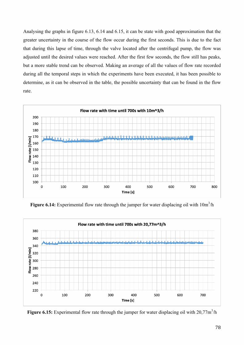
78

Analysing the graphs in figure 6.13, 6.14 and 6.15, it can be state with good approximation that the

greater uncertainty in the course of the flow occur during the first seconds. This is due to the fact

that during this lapse of time, through the valve located after the centrifugal pump, the flow was

adjusted until the desired values were reached. After the first few seconds, the flow still has peaks,

but a more stable trend can be observed. Making an average of all the values of flow rate recorded

during all the temporal steps in which the experiments have been executed, it has been possible to

determine, as it can be observed in the table, the possible uncertainty that can be found in the flow

rate.

Figure 6.14: Experimental flow rate through the jumper for water displacing oil with 10m3/h

Figure 6.15: Experimental flow rate through the jumper for water displacing oil with 20,77m3/h

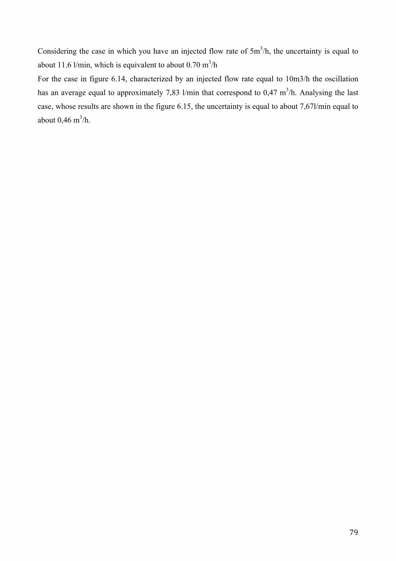
79

Considering the case in which you have an injected flow rate of 5m3/h, the uncertainty is equal to

about 11.6 l/min, which is equivalent to about 0.70 m3/h

For the case in figure 6.14, characterized by an injected flow rate equal to 10m3/h the oscillation

has an average equal to approximately 7,83 l/min that correspond to 0,47 m3/h. Analysing the last

case, whose results are shown in the figure 6.15, the uncertainty is equal to about 7,67l/min equal to

about 0,46 m3/h.

80

6.4Comparisonofresults

After having previously discussed the mathematical model and the LedaFlow results, it is now possible to compare these evidences with the results obtained in the laboratory, and assess the accuracy of the numerical model

For the first case of an injected flow rate of 5m3/h, as it can be seen in the figure 6.16, the first two experimental data points show a greater presence of oil in the jumper compared to the three simulations. The three following data points between 150 seconds and 400 seconds, instead, seem to be close to the results of the mathematical model. The last value at 700 seconds is slightly different from the results obtained with the three models. The result obtained in the laboratory is greater than the mathematical model but less than the two models studied with LedaFlow.

Figure 6.16: Comparison results for water displace oil with a flow rate of 5m3/h

In order to show even more clearly the results obtained, a comparison was made between the

complete configuration model created with LedaFlow and some photos taken in the laboratory. The

figure 6.17 shows that also in this case the model made with LedaFlow overestimates the presence

of oil inside the jumper compared to the experiments made in the laboratory. In the lower horizontal

part of the jumper the model estimates a greater presence of oil than that photographed at the same

time in the laboratory during the experiment.

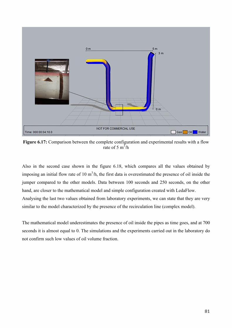
81


rate of 5 m3/h

Also in the second case shown in the figure 6.18, which compares all the values obtained by

imposing an initial flow rate of 10 m3/h, the first data is overestimated the presence of oil inside the

jumper compared to the other models. Data between 100 seconds and 250 seconds, on the other

hand, are closer to the mathematical model and simple configuration created with LedaFlow.

Analysing the last two values obtained from laboratory experiments, we can state that they are very

similar to the model characterized by the presence of the recirculation line (complex model).

The mathematical model underestimates the presence of oil inside the pipes as time goes, and at 700

seconds it is almost equal to 0. The simulations and the experiments carried out in the laboratory do

not confirm such low values of oil volume fraction.

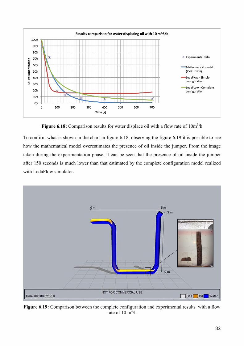
82

Figure 6.18: Comparison results for water displace oil with a flow rate of 10m3/h

To confirm what is shown in the chart in figure 6.18, observing the figure 6.19 it is possible to see

how the mathematical model overestimates the presence of oil inside the jumper. From the image

taken during the experimentation phase, it can be seen that the presence of oil inside the jumper

after 150 seconds is much lower than that estimated by the complete configuration model realized

with LedaFlow simulator.


rate of 10 m3/h

83

The last comparison is the one between all the simulations and the data from the laboratory for the

case in which a flow rate equal to 20,77 m3/h is injected.

It is possible to see that the first data found in the laboratory is probably a little closer to the data

obtained with simple simulation. The other five data obtained from laboratory experiments, instead,

seem to confirm almost perfectly the trend of the mathematical model and complex configuration.

Figure 6.20: Comparison results for water displace oil with a flow rate of 20,77m3/h

The amount of oil volume fraction estimated by the complete configuration with an injected flow

rate of 20,77 m3/h is closer to the results obtained in the laboratory, despite the image 6.21 shows

that even in this case the results of oil volume fraction obtained with LedaFlow are higher than the

actual amount of oil present during the experiments in the U-shaped jumper.

84


rate of 20,77m3/h

Analyzing all three charts it can be stated that the simple configuration, in the final part of the

simulation, tends to overestimate, compared to the other two models and the laboratory results, the

presence of oil inside the jumper.

On the contrary, the mathematical model, at least for the first two cases, is underestimated,

especially in the final part of the simulation, the presence of oil inside the jumper.

85

7.Conclusions

The displacement process of oil with water and water with oil in a U-shaped pipe geometry was

reproduced experimentally and numerically with a commercial simulator and an ideal mixing

model. The numerical results were in fair agreement with the experimental measurements.

According to the results of the numerical simulations, the flushing configuration without a

recirculation line allows to flush faster the fluid initially present in the pipe, when compared against

the configuration with the recirculation line. However, the amount of residual fluid in the jumper is

highly dependent on the flushing flow rate. The configuration with the recirculation line allows to

reach lower residual content of the initial fluid with lower injection rates.

According to numerical simulations of the configuration without recirculation line, a higher

flushing flow rate is required when flushing water with oil than for flushing oil with water to

achieve a low volume fraction of the initial fluid in the geometry.

Considering numerical simulations and experimental measurements of the configuration with

recirculation line, the flow rate through the geometry in displacement process does not vary

significantly during most of the displacement process.

Taking into account numerical simulations of the configuration with recirculation line, the

magnitude of the flow rate through the geometry does not affect significantly the efficiency of the

flushing process, within the ranges studied.

86

8.References

• Dr Najam Beg, Sacha Sarshar 2014. Surface Jet Pump (SJP) for Enhanced Oil & Gas

Production. Caltec Edition.

• Exxol D60 Fluid Product Safety Sumary, ExxonMobil Chemicals. Available at:

https://www.exxonmobilchemical.com/en/library/asset/80bd83e1923cfd9c85257762004897

fb

• Falcone, G., Hewitt, G. F. and Almonti, C. (2009) Multiphase Flow Metering. Elsevier.

• Folde, H. G. 2017. Experimental and Numerical Study of Fluid Displacement in Subsea

Pipe Sections. NTNU.

• GE Measurement and control (2011), UNIK5000 Pressure sensor platform. Available at:

https://www.gemeasurement.com/sites/gemc.dev/files/unik_5000_series_datasheet_italiano.

pdf

• GEA Liquid jet Liquid pump specification. Available at:

https://www.gea.com/it/productgroups/pumps_valves/jet-pumps/index.jsp

• I.J. Karassic, J.P. Messina, P. Cooper, C.C. Heald, Pump Handbook, Fourth edition,

McGraw-Hill, NY, 2008.

• J.Falcimaigne, S.Decarre, Multiphase production, Pipeline Transport, Pumping and

Metering, IFP Publications, T Editions Technip.

• KONGSBERG 2015a. LedaFlow Advanced Transient Multiphase Flow Simulator.

• KONGSBERG (2015b) LedaFlow user manual.

• KONGSBERG 2016a. LedaFlow 2.0 - The Advanced Transient Multiphase Flow Simulator.

• KONGSBERG (2016b) 'LedaFlow Getting Started'.

• KONGSBERG Group, LedaFlow software, 2017. Available at:

https://kongsberg.com/en/kongsberg-

digital/oil%20and%20gas/flow%20assurance/ledaflow%20software%20-page/

• Lenntech, Centrifugal pump Grundfos CRNE15 – 04. Available at:

https://www.lenntech.fr/grundfos/CRNE15/99071606/CRNE-15-4-A-FGJ-A-E-HQQE.html

• Nixon NT48-2” Turbine flow meter 110/1100 litres/min. Available at:

https://nixon.stockshed.com/index.php?route=product/product&manufacturer_id=14&produ

ct_id=237&page=2

• Offshore (2016) Subsea Production Systems Collection. Tulsa: PennWell Corporation. Available at: https://www.offshore-mag.com/learning-center/subsea/subsea-processing-collection/subsea-processing-maps-and-posters.html

87

• Opstvedt, J. A. K. 2016. Experiments and Numeric Simulation on Displacement and

Flushing of Hydrocarbon Fluid in Subsea Systems. NTNU.

• Society of Petroleum Engineering (SPE), Petrowiki, Subsea process benefits.

Available at: https://petrowiki.org/Subsea_processing_benefits

• The Engineering Toolbox (2017) Water – Thermodynamic Properties. Available at:

https://www.engineeringtoolbox.com/water-dynamic-kinematic-viscosity-d_596.html

• The Engineering Toolbox (2016f) Thermoplastics - Physical Properties. Available at:

https://www.engineeringtoolbox.com/physical-properties-thermoplastics-d_808.html

• The Engineering Toolbox (2016e) Thermal Expansion of PVC, CPVC, Carbon Steel,

Stainless Steel and Fiberglass Pipes. Available at:

https://www.engineeringtoolbox.com/thermal-expansion-pvc-d_782.html

• http://www.ledaflow.com

• Yong Bai, Qiang Bai, Subsea Engineering Handbook, Elsevier, 2012.

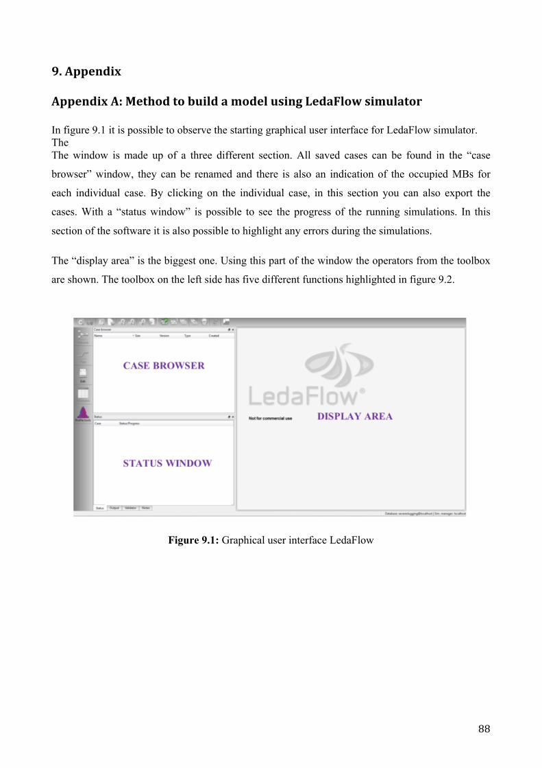
88

9.AppendixAppendixA:MethodtobuildamodelusingLedaFlowsimulatorIn figure 9.1 it is possible to observe the starting graphical user interface for LedaFlow simulator. TheThe window is made up of a three different section. All saved cases can be found in the “case

browser” window, they can be renamed and there is also an indication of the occupied MBs for

each individual case. By clicking on the individual case, in this section you can also export the

cases. With a “status window” is possible to see the progress of the running simulations. In this

section of the software it is also possible to highlight any errors during the simulations.

The “display area” is the biggest one. Using this part of the window the operators from the toolbox

are shown. The toolbox on the left side has five different functions highlighted in figure 9.2.

Figure 9.1: Graphical user interface LedaFlow

89

Figure 9.2: Function of the toolbox (KONGSBERG, 2016b)

One of the first steps to start working on a new case is to right-click in the case browser window. At

the beginning the user can choose between a default case of a simple case. The default case is

characterized by the fact that it has 2 phases (liquid-gas) or 3 phases (water-oil-gas) that is

composed of a 300-meter horizontal line with default properties.

In order to set a specific case simply clicks on the blue symbol highlighted in the figure 9.3.

Figure 9.3: Graphical user interface LedaFlow By clicking on the highlighted symbol, the window in figure 9.4 will appear, which is useful for

setting the characteristic parameters such as temperature and pressure, thermal option and some

other parameter useful to the simulation of flow assurance (emulsion, pigging, hydrate

characteristics, etc.).

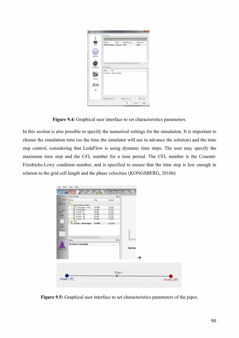
90

Figure 9.4: Graphical user interface to set characteristics parameters. In this section is also possible to specify the numerical settings for the simulation. It is important to

choose the simulation time (so the time the simulator will use to advance the solution) and the time

step control, considering that LedaFlow is using dynamic time steps. The user may specify the

maximum time step and the CFL number for a time period. The CFL number is the Courant-

Friedrichs-Lewy condition number, and is specified to ensure that the time step is low enough in

relation to the grid cell length and the phase velocities (KONGSBERG, 2016b).

Figure 9.5: Graphical user interface to set characteristics parameters of the pipes.

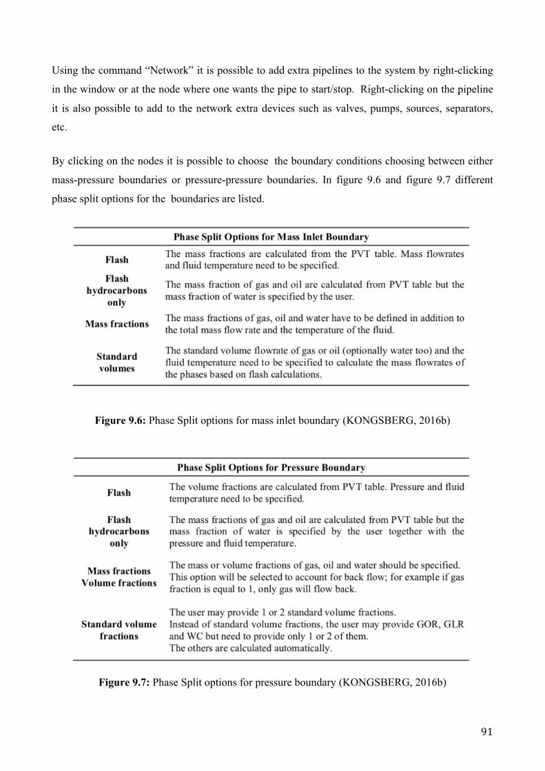
91

Using the command “Network” it is possible to add extra pipelines to the system by right-clicking

in the window or at the node where one wants the pipe to start/stop. Right-clicking on the pipeline

it is also possible to add to the network extra devices such as valves, pumps, sources, separators,

etc.

By clicking on the nodes it is possible to choose the boundary conditions choosing between either

mass-pressure boundaries or pressure-pressure boundaries. In figure 9.6 and figure 9.7 different

phase split options for the boundaries are listed.

Figure 9.6: Phase Split options for mass inlet boundary (KONGSBERG, 2016b)

Figure 9.7: Phase Split options for pressure boundary (KONGSBERG, 2016b)

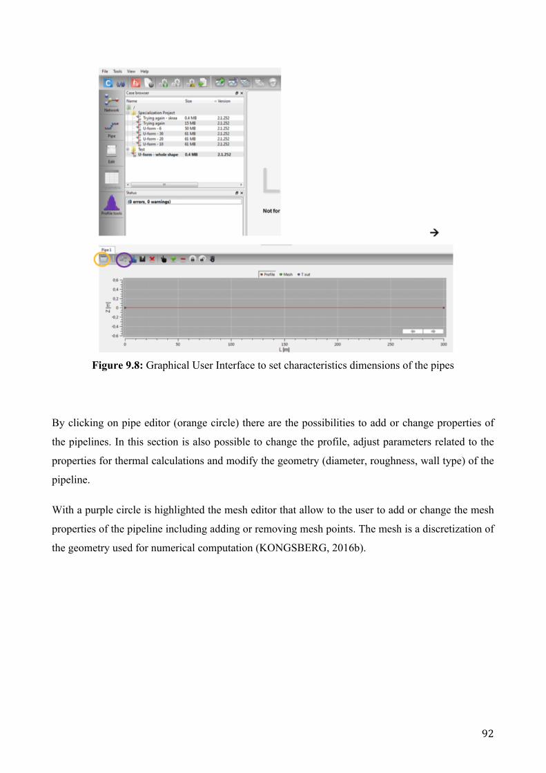
92

Figure 9.8: Graphical User Interface to set characteristics dimensions of the pipes

By clicking on pipe editor (orange circle) there are the possibilities to add or change properties of

the pipelines. In this section is also possible to change the profile, adjust parameters related to the

properties for thermal calculations and modify the geometry (diameter, roughness, wall type) of the

pipeline.

With a purple circle is highlighted the mesh editor that allow to the user to add or change the mesh

properties of the pipeline including adding or removing mesh points. The mesh is a discretization of

the geometry used for numerical computation (KONGSBERG, 2016b).

ALMA MATER STUDIORUM - UNIVERSITÀ DI BOLOGNA

Documents

Transcript of ALMA MATER STUDIORUM - UNIVERSITÀ DI BOLOGNA