1228 IEEE TRANSACTIONS ON MEDICAL IMAGING, VOL. 30, NO. 6, JUNE 2011

Aligning Scan Acquisition Circles in OpticalCoherence Tomography Images of

The Retinal Nerve Fibre LayerHaogang Zhu, David P Crabb*, Patricio G Schlottmann, Gadi Wollstein, and David F Garway-Heath

Abstract—Optical coherence tomography (OCT) is widely usedin the assessment of retinal nerve fibre layer thickness (RNFLT)in glaucoma. Images are typically acquired with a circular scanaround the optic nerve head. Accurate registration of OCT scans isessential for measurement reproducibility and longitudinal exam-ination. This study developed and evaluated a special image regis-tration algorithm to align the location of the OCT scan circles tothe vessel features in the retina using probabilistic modelling thatwas optimised by an expectation-maximization algorithm. Evalua-tion of the method on 18 patients undergoing large number of scansindicated improved data acquisition and better reproducibility ofmeasured RNFLT when scanning circles were closely matched. Theproposed method enables clinicians to consider the RNFLT mea-surement and its scan circle location on the retina in tandem, re-ducing RNFLT measurement variability and assisting detection ofreal change of RNFLT in the longitudinal assessment of glaucoma.

Index Terms—Expectation-maximization, image registration,optical coherence tomography, probabilistic modelling, scan circlealignment.

I. INTRODUCTION

G LAUCOMA is a leading cause of irreversible visual im-pairment, being a progressive optic neuropathy resulting

in the loss or damage of retinal ganglion cells (RGCs) and their

Manuscript received December 12, 2010; revised January 16, 2011; acceptedJanuary 18, 2011. Date of publication February 04, 2011; date of current versionJune 02, 2011. This work was supported by an unrestricted investigator initiatedresearch grant from Pfizer Inc., an unrestricted educational grant from OptovueInc., and in part by the Department of Health’s NIHR (National Institute ofHealth Research) Biomedical Research Centre for Ophthalmology at MoorfieldsEye Hospital and UCL Institute of Ophthalmology. The views expressed in thepublication are those of the authors and not necessarily those of the Departmentof Health. D. F. Garway-Heath’s Chair at UCL is supported by funding from theInternational Glaucoma Association. Asterisk indicates corresponding author.

H. Zhu is with the Department of Optometry and Visual Science, City Uni-versity London, EC1V 0HB London, U.K., and also with the National Institutefor Health Research Biomedical Research Centre for Ophthalmology, Moor-fields Eye Hospital National Health Service Foundation Trust and UniversityCollege London Institute of Ophthalmology, EC1V 2PD London, U.K. (e-mail:haogangzhu@gmail.com).

*D. P. Crabb is with the Department of Optometry and Visual Science, CityUniversity London, EC1V 0HB London, U.K. (e-mail: d.crabb@city.ac.uk).

P. G. Schlottmann is with the National Institute for Health Research Biomed-ical Research Centre for Ophthalmology, Moorfields Eye Hospital NationalHealth Service Foundation Trust and University College London Institute ofOphthalmology, EC1V 2PD London, U.K. (e-mail: schlottp@yahoo.com.ar).

G. Wollstein is with the Eye Center of University of Pittsburgh MedicalCenter, Department of Ophthalmology, University of Pittsburgh, Pittsburgh,PA 15213 USA (e-mail: wollsteing@upmc.edu).

D. F. Garway-Heath is with the National Institute for Health ResearchBiomedical Research Centre for Ophthalmology, Moorfields Eye Hospital NHSFoundation Trust and University College London Institute of Ophthalmology,EC1V 2PD London, U.K. (e-mail: david.garway-heath@moorfields.nhs.uk).

Color versions of one or more of the figures in this paper are available onlineat http://ieeexplore.ieee.org.

Digital Object Identifier 10.1109/TMI.2011.2109962

axons. In human eyes, light rays are focused and sensed on theretina, which is the tissue layer at the back of the eye. Simplyput, the top “layer” of the retina consists of RGCs and theiraxons (nerve fibres) with photoreceptors (rods and cones) un-derneath. The retinal nerve fibres converge to form the opticnerve head (ONH) where they exit the eye to enter the brain.The retinal nerve fibres carry the signals from across the retinainto the brain so the damage or “thinning” of RGCs and theiraxons caused by glaucoma results in the irreversible visual im-pairment.

Estimates of RGC axon loss can be made by the surrogatemeasurement of retinal nerve fibre layer (RNFL) thicknessusing modern imaging techniques such as optical coherencetomography (OCT) [1], [2]. Similar to ultrasound technique,OCT detects the backscattered light from the retina and pro-duces high resolution, cross-sectional images. This techniquehas formed time-domain OCT (TD-OCT) systems such as theStratusOCT (Carl Zeiss Meditec, Inc., Dublin, CA) that hasbeen successfully used in the clinic as a clinical standard formeasuring the RNFL thickness (RNFLT) in glaucoma in recentyears [3]–[7]. In the StratusOCT system, measurement of theretinal layers is acquired by an axial-scan in depth (A-scan) anda cross-sectional scan (B-scan). The A-scans are sampled undera scan circle (typical diameter of 3.4 mm) which is manuallycentred on the ONH [Fig. 1(i)] as guided by a “live” imageof the fundus but the location of the scan circle is unknownduring the image acquisition. The RNFLT is then analysedby segmentation algorithms provided by the software. Onedifficulty during image acquisition is the displacement of thecircular scan due to the operator’s subjective placement of thescan circle or the eye movement after the manual adjustment.This displacement means that the RNFLT is not necessarilysampled at the same location and this contributes to the vari-ability and error in the measurement [8]–[10], restricting theuse of the technique especially in determining the deteriorationof the RNFLT in the longitudinal assessment or follow-up ofglaucoma. Moreover, the problem of RNFLT reproducibilitydue to image acquisition difficulties was also recently identifiedas a limiting factor for this technology in the diagnosis ormanagement of multiple sclerosis [11]. Therefore, a method foridentifying and aligning the location of the scan circle wouldbe clinically useful as it may offer better tracking of the samearea of RNFLT over time.

Newer spectral-domain OCT (SD-OCT) [12], [13] operateswith faster scans [14] giving improved signal-to-noise ratio inthe measurements [15], [16] compared to TD-OCT. Althoughsome commercially available SD-OCT (e.g., Cirrus, Carl Zeiss

0278-0062/$26.00 © 2011 IEEE

ZHU et al.: ALIGNING SCAN ACQUISITION CIRCLES IN OPTICAL COHERENCE TOMOGRAPHY IMAGES OF THE RETINAL NERVE FIBRE LAYER 1229

Meditec, CA) scan protocols extract the circular scan from a 3Dvolume scan, most other SD-OCT systems (e.g., RTVue-100,Optovue, Fremont, CA) still provide circular scan as one of thescan protocols or include circular scans in more complex pro-tocols (e.g., RTVue-100 NHM4 protocol consisting of 6 circleand 12 line scans) so they may still be affected by displacementbetween scans [8], [17]. Therefore, improvements in this imageacquisition protocol, or at least knowing the area of RNFLT thathas been acquired, will still be beneficial for SD-OCT deviceswith such scan acquisition protocols. Moreover, TD-OCT hasbeen used to follow up the progression of glaucoma long be-fore the emergence of the SD-OCT, and it is still widely usedby glaucoma services where clinicians (or research study co-or-dinators) are reluctant to abandon series of data collected withTD-OCT over time since this provides important informationabout the longitudinal characteristic of glaucoma. The methodproposed in this study may facilitate migration from TD-OCTto SD-OCT, for instance, by aligning TD-OCT scan circles onthe volumetric images acquired by SD-OCT, so that longitudinalseries are not wasted.

The effect of scan circle location on the RNFLT measure-ment has been previously investigated by simulating differentscan circle locations on a volumetric image around the ONHtaken by ultrahigh-resolution OCT [8]. The circular scans weresimulated by sampling the A-scans under a scan circle (3.4mm diameter) shifted with known displacements horizontally(x-shift), vertically (y-shift), and diagonally from the centerof the ONH. This method allowed for systematic investigationof the variable circle placement effect. The results from thisstudy clearly demonstrated that the location of the OCT scancircle adds substantial variability to the RNFLT measurements.Since registration of OCT scans is imperative for measurementreproducibility and longitudinal examination, it would be veryuseful to have a method that could estimate the location of thescan circle on the retina. Kim et al. [18] proposed a method toalign the circular scan image to a volumetric image around theONH acquired by SD-OCT by using simulated cross-sectionalimages under scan circles at various locations sampled fromthe volumetric image. The circular scan was then aligned tothe most similar sampled SD-OCT scans where the similaritywas assessed by cross correlation between retinal structuresin the A-scans from two images. One limitation is that thetechnique uses retinal structures that typically change duringthe worsening of glaucoma, giving it limited appeal in fol-lowing up RNFLT changes if the circular scan and volumetricscans are acquired in different periods of time. This approachmight help bridge the gap in RNFLT measurements betweenthe TD-OCT circular scan and the SD-OCT volumetric scan,providing longitudinal comparability. However this approachis only useful when both TD-OCT and SD-OCT are availableand it will not be helpful in a common situation where a clinicmight be following patients with TD-OCT technology alonefor years.

This study proposes a new OCT scan circle alignment algo-rithm using blood vessel features which are considered to berelatively stable landmarks when considering longitudinal im-ages in glaucoma. The algorithm can align multiple OCT cir-cular scans to a retinal fundus image that is generally available

Fig. 1. Retinal fundus image and OCT circular scan for the same eye. Thedetected vessels are modelled and delineated by cubic splines, shown here asred curves superimposed on the fundus image (I) and labelled with letters inuppercase (A–N). The image acquisition begins with a circle placed in an arbi-trary position around the ONH, e.g., the blue circle in (I). The scan starts fromthe mid-temporal area at 180 (blue arrow on scan circle) and traverses in aclock-wise direction to superior (90 ), nasal (0 ), inferior ��90 �, and finallyback to the mid-temporal area. The circular scan is “straightened” to a line (in2D) as shown in (II). The results of the OCT vessel detection technique are in-dicated in (II) as crosses and are superimposed as white circles in the fundusimage (I). The OCT vessels are numbered by letters in lowercase (a–j). The an-gular values of the indicated position of the OCT vessels and the intersectionsbetween the scan circle and fundus image vessels are plotted in (III). The linesin (III) link each OCT vessel to the nearest fundus image vessel.

in the glaucoma clinics from various imaging techniques, suchas scanning laser polarimetry (SLP), scanning laser ophthalmo-scope or even a fundus camera. The algorithm has been devel-oped to have general applicability to any type of fundus andOCT images but is demonstrated in this study on StratusOCTimages and fundus images acquired with SLP ( ; CarlZeiss Meditec, Inc., Dublin, CA). It has been successfully usedin a recent study that assessed the axonal birefringence of RNFLby aligning the OCT scan circle onto the SLP image [19].

II. METHODS

The proposed method aligns an OCT scan circle on the retinalfundus image by a registration technique using the blood vesselfeatures available in both types of images. The vessels in OCTimages typically appear as shaded bands along the retinal pig-ment epithelium [RPE; Fig. 1(ii)]. The RPE is detected as thetissue layer with the strongest intensity peaks in the OCT image.The “shaded band” feature of vessels is then detected as thelocal minimums on the averaged pixel intensities around theRPE [Fig. 1(ii)]. The vessel features in the retinal fundus im-ages differ with the imaging techniques used, and the vesselsegmentation in retinal images have been extensively studiedpreviously [20]–[25]. In the implementation of vessel detectionfor the SLP fundus image, a measure of “vesselness” serves asa preprocessing step for segmentation of vessels in the retinalfundus image. A technique using the multi-scale second orderlocal structure of an image [26] is used for this purpose. Thevessels are then analytically reconstructed using cubic splines[Fig. 1(i)] [27].

A scan circle around the ONH and the detected vessels inthe OCT (white circles superimposed on the blue scan circle)and fundus image (red lines) are shown in Fig. 1. That the scancircle is displaced is indicated by the poorly aligned vessels. The

1230 IEEE TRANSACTIONS ON MEDICAL IMAGING, VOL. 30, NO. 6, JUNE 2011

method proposed in this work infers the scan circle location byaligning the vessels from both images.

A. Problem Formalisation

In an acquisition of an OCT image (Fig. 1), the circular scanstarts from the mid-temporal area at 180 (blue arrow on scancircle in Fig. 1(i) and traverses in a clock-wise direction to su-perior (90 ), nasal (0 ), inferior 90 , and finally back to themid-temporal area. The circular scan is then “straightened” to a“line” in two dimensions [Fig. 1(ii)]. Each column in the OCTimage is therefore associated with an angular value on the scancircle. The locations of detected vessels in the OCT image areconverted to angular values [e.g., Fig. 1(iii)] and are denotedas where is the number of OCT vessels. The -and -coordinates of each vessel in the retinal fundus imageare expressed as two cubic splines [27], respectively, each ofwhich is essentially a piecewise function defined over a param-eter . The cubic spline has segments divided by knots

on and the one having an intersection with thescan circle is assumed to be the th segment, so the coordinate

of this segment of the th fundus image vessel are

(1)The location of a scan circle with radius mm is de-

fined by three parameters: center coordinate , and rotation(in degree) around the center. The circle rotation rotates all

OCT vessels around the scan circle center by degrees and, inthe “straightened” two dimensions image [Fig. 1(ii)], it shifts theOCT vessels (and the whole image) on horizontal by degrees.Given the parameters of a scan circle, the intersection betweena vessel defined by (1) and the scan circle can be calculated bysolving the following polynomial equation with respect to :

(2)

with the constraint and inserting the rootback to (1) to calculate the solutions of and . The angularvalue of the intersection is then calculated as

(3)for where is the number of vessels in thefundus image. is also used to represent the corre-sponding fundus image vessel.

The scan circle alignment can be decomposed into twotasks: vessel matching and displacement parameter inference.The vessel matching links an OCT vessel and a fundusimage vessel if they belong to a same vessel. Thedisplacement parameter inference infers the parametersand to minimize the distances between the matched vesselsin two images. These two steps are both nontrivial and affecteach other in a complex way. For instance, the OCT and fundusimage vessels in Fig. 1 cannot be matched without knowingthe location parameters. An OCT vessel cannot be simplymatched to the nearest fundus image vessel. In the examplein Fig. 1, the nearest-matching criterion [Fig. 1(iii)] resultsin obvious erroneous vessel pairs [c-C, f-J, i-M, and j-N inFig. 1(i)]. On the other hand, the displacement parameterscannot be inferred without knowing how the vessels in twoimages are matched. Because of the complicated interactionbetween vessel matching and parameter inference, treatingthem independently would result in suboptimal solutions.

B. Probabilistic Modelling

The complex relationship between vessel matching andscan circle displacement parameter inference is modelled witha probabilistic model with unobserved variables. The taskof vessel matching can be divided into two processes. First,whether the OCT vessel can be matched to a fundus imagevessel is examined. If this can be done accurately then aninference about what vessels in the fundus image it needsto be matched to. Two groups of unobserved variables areintroduced to model these two processes. The binary vector

is encoded with 1-out-of-2 notation inwhich only one of the two elements can be equal to 1 in :

if the th OCT vessel can be accurately aligned toa fundus image vessel, otherwise . A prior probabilityover is introduced such that foror 1 so

(4)

It is also required that probability values satisfy. Another binary vector adopts

1-out-of- notation so that only one of the elements incan be equal to 1, and indicates that the th OCT vesselis matched to the th fundus image vessel. Similarly, a priorprobability over is set as for toso

(5)

where are probability values satisfying .The posterior probability of given is defined as a

mixture of two Gaussian distributions centred on the same meanof but with different variance that is decided by thevalue of

(6)

ZHU et al.: ALIGNING SCAN ACQUISITION CIRCLES IN OPTICAL COHERENCE TOMOGRAPHY IMAGES OF THE RETINAL NERVE FIBRE LAYER 1231

where the parameters are set to satisfy . Thiscan be interpreted as if the OCT vessel can be accuratelyaligned to the fundus image vessel , then

needs to be close to in order to “score” a highprobability, otherwise a small divergence (defined by smallsuch as 2 ) from would result in a probability nearto zero. On the other hand, if the OCT vessel cannot beaccurately aligned to a fundus image vessel ,distributes more “uniformly” (defined by large such as 45 )with a small probability value, so the divergence fromhas minimal effect on the probability.

From (6), the posterior probability can be de-fined as

(7)from which the joint probability can be calculatedas the multiplication of (4), (5) and (7)

(8)

The joint probability defines a mixture ofGaussian mixture. This “mixture of mixture” model structurewas previously used for classification problems [28] and inother applications where the model was named after “com-pound mixture model” [29].

Because and are all unobserved variablesas opposed to directly observed variables, the likelihood can becalculated by marginalizing the joint probability over these un-observed variables and assuming that are independentand identically distributed

(9)

Because only one element in vectors and can be equalto “1” respectively, the summation and multiplicationover and in the first step of (9) represent the exhaustive sum-mation of all possible over and

. Therefore, in the second step, and the multiplicationover and are substituted with the summation over and .

C. Expectation-Maximization Algorithm

An expectation-maximization (EM) algorithm [30] is used forfinding maximum likelihood estimates of the parameters in (9).

In the expectation (E) step, the posterior probability of the un-observed variables is calculated as

(10)

by using (8) and the th component in (9). The expectations ofand with respect to the distribution

are then calculated in the E-step and will be used in the fol-lowing maximization (M) step, which computes parametersmaximizing the expected complete log likelihood found in theE step

(11)

and

(12)

In the M-step, the expectation of the complete likelihoodunder the distribution of is cal-

culated and maximized with respect to the parameters , ,and

(13)

where (11) and (12) have been used. This target function is di-vided into three components each of which contains a group ofthe parameters. Note that the components of this function thatdo not include any parameters were grouped into a constant termas they are irrelevant to the maximization of the objective func-tion.

1232 IEEE TRANSACTIONS ON MEDICAL IMAGING, VOL. 30, NO. 6, JUNE 2011

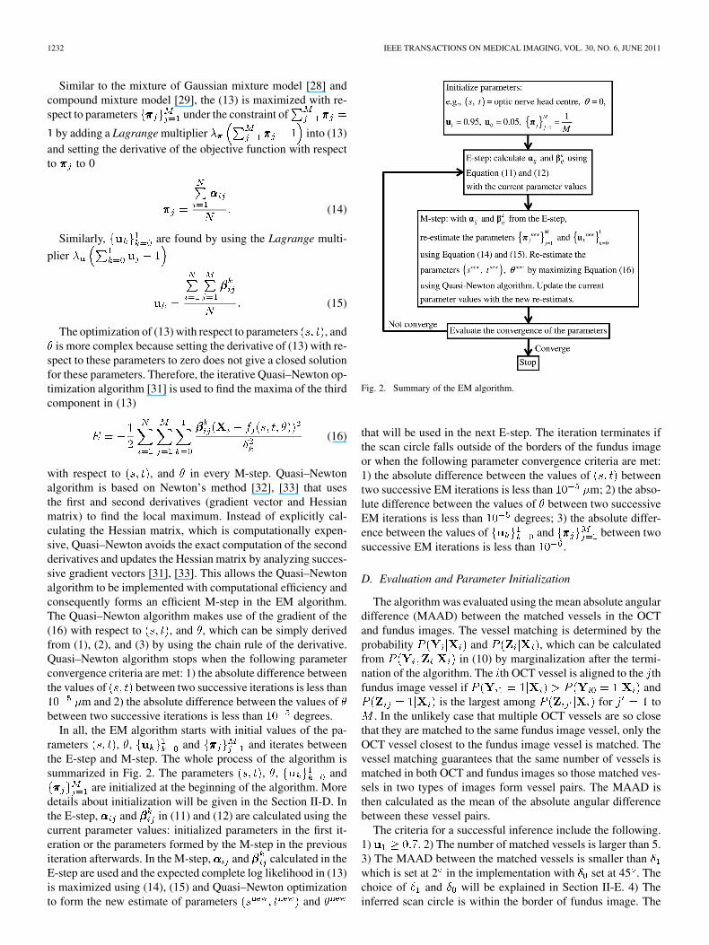
Similar to the mixture of Gaussian mixture model [28] andcompound mixture model [29], the (13) is maximized with re-spect to parameters under the constraint of

by adding a Lagrange multiplier into (13)and setting the derivative of the objective function with respectto to 0

(14)

Similarly, are found by using the Lagrange multi-

plier

(15)

The optimization of (13) with respect to parameters , andis more complex because setting the derivative of (13) with re-

spect to these parameters to zero does not give a closed solutionfor these parameters. Therefore, the iterative Quasi–Newton op-timization algorithm [31] is used to find the maxima of the thirdcomponent in (13)

(16)

with respect to , and in every M-step. Quasi–Newtonalgorithm is based on Newton’s method [32], [33] that usesthe first and second derivatives (gradient vector and Hessianmatrix) to find the local maximum. Instead of explicitly cal-culating the Hessian matrix, which is computationally expen-sive, Quasi–Newton avoids the exact computation of the secondderivatives and updates the Hessian matrix by analyzing succes-sive gradient vectors [31], [33]. This allows the Quasi–Newtonalgorithm to be implemented with computational efficiency andconsequently forms an efficient M-step in the EM algorithm.The Quasi–Newton algorithm makes use of the gradient of the(16) with respect to , and , which can be simply derivedfrom (1), (2), and (3) by using the chain rule of the derivative.Quasi–Newton algorithm stops when the following parameterconvergence criteria are met: 1) the absolute difference betweenthe values of between two successive iterations is less than

m and 2) the absolute difference between the values ofbetween two successive iterations is less than degrees.

In all, the EM algorithm starts with initial values of the pa-rameters , , and and iterates betweenthe E-step and M-step. The whole process of the algorithm issummarized in Fig. 2. The parameters , , and

are initialized at the beginning of the algorithm. Moredetails about initialization will be given in the Section II-D. Inthe E-step, and in (11) and (12) are calculated using thecurrent parameter values: initialized parameters in the first it-eration or the parameters formed by the M-step in the previousiteration afterwards. In the M-step, and calculated in theE-step are used and the expected complete log likelihood in (13)is maximized using (14), (15) and Quasi–Newton optimizationto form the new estimate of parameters and

Fig. 2. Summary of the EM algorithm.

that will be used in the next E-step. The iteration terminates ifthe scan circle falls outside of the borders of the fundus imageor when the following parameter convergence criteria are met:1) the absolute difference between the values of betweentwo successive EM iterations is less than m; 2) the abso-lute difference between the values of between two successiveEM iterations is less than degrees; 3) the absolute differ-ence between the values of and between twosuccessive EM iterations is less than .

D. Evaluation and Parameter Initialization

The algorithm was evaluated using the mean absolute angulardifference (MAAD) between the matched vessels in the OCTand fundus images. The vessel matching is determined by theprobability and , which can be calculatedfrom in (10) by marginalization after the termi-nation of the algorithm. The th OCT vessel is aligned to the thfundus image vessel if and

is the largest among for to. In the unlikely case that multiple OCT vessels are so close

that they are matched to the same fundus image vessel, only theOCT vessel closest to the fundus image vessel is matched. Thevessel matching guarantees that the same number of vessels ismatched in both OCT and fundus images so those matched ves-sels in two types of images form vessel pairs. The MAAD isthen calculated as the mean of the absolute angular differencebetween these vessel pairs.

The criteria for a successful inference include the following.1) . 2) The number of matched vessels is larger than 5.3) The MAAD between the matched vessels is smaller thanwhich is set at 2 in the implementation with set at 45 . Thechoice of and will be explained in Section II-E. 4) Theinferred scan circle is within the border of fundus image. The

ZHU et al.: ALIGNING SCAN ACQUISITION CIRCLES IN OPTICAL COHERENCE TOMOGRAPHY IMAGES OF THE RETINAL NERVE FIBRE LAYER 1233

Fig. 3. The mean MAAD and � under different values of � .

first two criteria ensure that the inferred scan circle displace-ment is “agreed” by adequate number of vessels. The third cri-terion guarantees that the distance between the matched vesselsis sufficiently small.

Without losing generalization, the parameters ,and are initialized to be , ,and . The choice of results from theexpectation that most OCT vessels can be aligned to the fundusimage vessels. There are multiple initialization options forthe parameters in order to cope with the potential largedisplacement of scan circles: they are initialized to be at ninelocations shifted by 0 and m from the center of the ONHon both the - and -axis. The algorithm starts with differentparameter initialization and if the inferred values of parametersare different with different initialization, the displacement ischosen as the one with the lowest MAAD from a successfulinference.

E. Choice of and

The parameters and were set such that . Quan-titatively, it was defined that the two intersections between thetwo Gaussian distributions defined by and in (6) are 2.5from the mean. Therefore, given the value of , can be calcu-lated thereafter. To find the optimal , various values of areused and the mean MAAD and mean are examined (Fig. 3).To illustrate the effect of , the first two criteria of successfulinference are not used because, as it will be shown below, fewer

OCT vessels can be matched to the fundus imagevessels with small values.

defines the necessary “closeness” of the OCT vessel to thefundus image vessel in order to match the two vessels. As shownin Fig. 3(a), small allows for a smaller difference betweenthe OCT and fundus image vessels and thus gives better (lower)MAAD for the matched vessels. However, smaller also ex-cludes more OCT vessels so fewer OCT vessels can be matchedto the fundus image vessels, which is quantified by lower valueof [Fig. 3(b)]. For instance, although gives a lowmean MAAD of 0.29 , less than 70% of the OCT

vessels can be matched to the fundus image vessels. On the otherhand, large allows for more OCT vessels to be matched to thefundus image vessels but the MAAD also increases at the sametime.

Therefore, the choice of reflects the trade-off betweenlower MAAD and having adequate number of matched vessels.In this implementation, is chosen as the value giving thelowest mean MAAD with mean as required by thecriteria of successful inference. This value of was found tobe 2 , and was calculated to be 45 .

F. Validation Experiments

The OCT scan circle alignment algorithm was developed andimplemented in MATLAB (ver. 7.9.0 R2009b, The MathWorks,Inc., Natick, MA). An executable version of this software isfreely available from the authors.

The algorithm was initially developed using StratusOCTdata from patients with glaucoma made available from the EyeCenter of University of Pittsburgh Medical Center (data notshown) [18], [34]. The algorithm was then validated by inves-tigating the impact of scan circle displacement on the RNFLTmeasurement repeatability using a separate dataset acquiredfor the purpose from Moorfields Eye Hospital National HealthService Trust, London, U.K. Eighteen patients (mean age of 65(range 50–82) years) with a clinical diagnosis of glaucomatousoptic neuropathy (primary open angle or normal tension glau-coma) with reproducible visual field defects were recruited.The study was approved by an ethics committee and informedconsent, according to the tenets of the Declaration of Helsinki,was obtained prior to examination from each subject. In thestudy protocol, a chosen eye from each subject was imaged 23times with the StratusOCT system using the Fast RNFL Thick-ness (3.4) protocol. This protocol acquired three consecutivesingle scans in one image acquisition giving 69 single scansfor each eye. Fundus images were acquired with the GDxVCCwhich covers an area of 5.9 mm 5.9 mm around the ONH.Patient identifiers were removed from the data before beingtransferred to a secure database at City University London.

1234 IEEE TRANSACTIONS ON MEDICAL IMAGING, VOL. 30, NO. 6, JUNE 2011

Fig. 4. An example of OCT scan circle alignment algorithm. The initial location of the OCT scan circle and its vessels were described in Fig. 1(i) and the initialrotation was 0 . The OCT scan circle and its vessels were superimposed on the fundus image (I) at the inferred center (black dot) and rotation (3.5 ). The pathof the scan circle center at each step of the EM algorithm was plotted as a black curve on the fundus image. The posterior probability � �� � ��� � and� �� �� � for the matched vessel is denoted in the bracket beside each OCT vessel in the format of (� �� � ��� �, matched vessel pair: � �� �� �).

III. RESULTS

The algorithm was used to align all 69 OCT circular scansonto the corresponding fundus images for each eye. On average,the EM algorithm took 10.3 iterations before convergence. Ineach M-step, the average number of Quasi–Newton optimisa-tion was 23.2. Computational time for aligning each OCT scancircle to the fundus image was 2.3 s (SD 0.6 s) on a typicaldesktop PC with one core of Intel Core 2 Due 2.53 GHz CPUand 2 GB RAM.

A. Algorithm Performance

An example of the results from the alignment algorithm forone of the eyes is shown in Fig. 4. The initial location of the OCTcircular scan and its vessels are described in Fig. 1(i). The EMalgorithm took 11 iterations to estimate the location of the scancircle in this example. Relative rotation of this scan circle withrespect to the fundus image was 3.5 and was corrected whenplotting the OCT vessels in Fig. 4(i). The algorithm was suc-cessful in aligning the vessels in the images and this is quantifiedby the MAAD between the matched vessels having a relativelysmall value of 0.4 . In this example, most OCT vessels (froma to i) could be aligned to the fundus image vessels, as indi-cated by the large posterior probabilities whichare also given in Fig. 4(i). On the other hand, one OCT vessel(j) could not be aligned to any fundus image vessel because inthis case . The OCT image in Fig. 1(ii)shows that the detection of this “vessel” may be a false posi-tive result by the OCT vessel detection algorithm because it isnot clear from looking at the image alone that there should be avessel at that location. The vessel matching was decided by thelargest posterior probabilities among for to

which were denoted in Fig. 4(i).The algorithm produced successful inference of scan circle

displacement for all OCT images. On average, the mean andSD of MAAD for all OCT circular scans in thissample of eyes were . The average number of de-tected vessels in these OCT images was 11.6. On average, 86%

of the OCT vessels could be aligned to fundus images with pos-terior probabilities . There-fore, the average number of matched vessels is 10 ,suggesting that, although 14% of the vessels were not matched,the algorithm could terminate with successful inference (criteriadescribed in Section II-D) “agreed” by the majority of the ves-sels and was able to align the OCT vessels to the fundus imagevessels with minimal angular difference.

Locations of 69 repeated circular scans from the same ex-ample eye are shown in Fig. 4(ii). Although the operator aimedto scan the same circular area on the retina, the scan circles,as inferred by the algorithm, are displaced from each other andcovered a wide annulus area around the ONH. The distance (rel-ative shift in microns and as degrees of relative rotation) be-tween the center of each scan circle, as determined by the algo-rithm, was calculated for all possible pairs of scans .In the example shown in Fig. 4, the mean distance between twoscan circles was 143 m (SD of 130 m) and relative rotationwas 1.9 (SD of 1.8 ).

During the OCT image acquisition, three scans are taken con-secutively within 1.92 s after the manual placement of scancircle so the locations of the scan “triplet” are expected to be af-fected less by the circle placement. To examine the assumption,the relative distances on the -axis, -axis, the overall distancesin microns and the rotational distances in degree between allpairs of scan circles were calculated for each eye. These dis-tances were compared with those calculated with scan circlepairs from three consecutive scans during the same image acqui-sition. The mean and SD of these distances were summarized inTable I, showing that, on average, the distance between two cir-cular scans tends to be smaller if they belong to the scan tripletfrom the same image acquisition.

B. Effect of Scan Circle Displacement on RNFLT

The impact of scan circle displacement on RNFLT mea-surement was examined. Quadrant RNFLT measurements(temporal, superior, nasal, and inferior) were plotted against

-axis and -axis displacements of the center of each scan

ZHU et al.: ALIGNING SCAN ACQUISITION CIRCLES IN OPTICAL COHERENCE TOMOGRAPHY IMAGES OF THE RETINAL NERVE FIBRE LAYER 1235

TABLE IDISTANCES AND ROTATION DIFFERENCE ����� � ��� BETWEEN

TWO CIRCULAR SCANS

Fig. 5. Plot of quadrant RNFLT measurements against the scan circle centerlocations on �- and �-axis from one eye with fitted linear regression lines. Theorigin point (0 �m) of the scan circle center was arbitrarily chosen within theONH. The slopes of the lines all differ from �� � ��.

circle. Linear regression then gave estimates of the averagechange of quadrant RNFLT caused by the displacement of scancircle. An example from one eye is shown in Fig. 5.

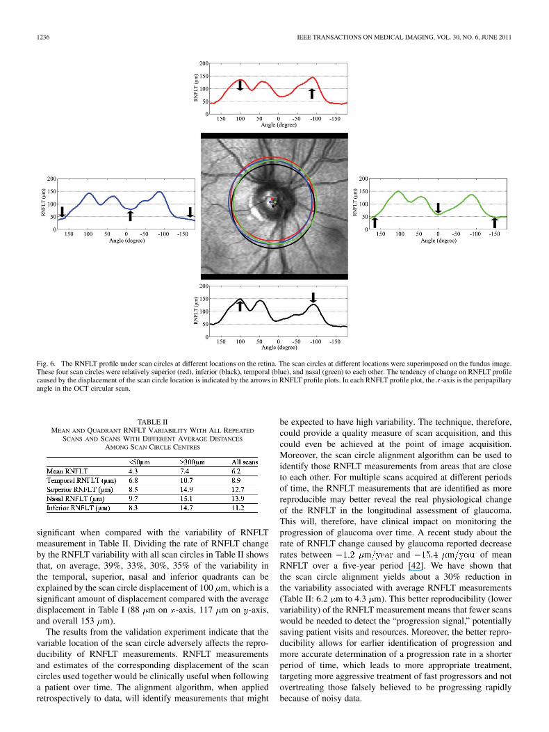
The superior and nasal RNFLT are negatively correlated withthe scan circle location on - and -axis, respectively. Similarlythe inferior and temporal RNFLT are positively correlated withthe scan circle location on - and -axis, respectively. On av-erage, the inferior RNFLT increases by m and thesuperior RNFLT decreases by m when the -coor-dinate of scan circle center increases by 100 m; the temporalRNFLT increases by m and the nasal RNFLT de-creases by m when the -coordinate of scan circlecenter increases by 100 m.

The impact of scan circle displacement on RNFLT can alsobe observed by the change of RNFLT profile under scan circlesat different locations. Fig. 6 shows four scan circles relativelydisplaced towards superior, inferior, temporal, and nasal direc-tions. Note that the RNFLT profiles feature a “double hump”shape where the RNFLT in superior and inferior areas is thickerthan that in temporal and nasal regions. It is clear that movingthe scan circle inferiorly increases the superior RNFLT and de-creases the inferior RNFLT, and vice versa. Similarly, the scancircle on the nasal side has relatively thicker temporal RNFLT

and thinner nasal RNFLT compared with the scan circle on thetemporal side.

C. RNFLT Measurement Variability

The RNFLT change caused by the scan circle displacementcontributes to the variability of RNFLT measurement. The effectof scan circle displacement on mean and quadrant RNFLT mea-surement variability was investigated. Variability was scored astwo times the standard deviation of three repeated scans [35],which were drawn from the exhaustive combination of all re-peated scans of each eye. The average variability was calculatedwith all repeated scans and those scans with average distanceamong scan circle centres smaller than 50 m and larger than300 m (Table II). In short, the former represent a group of cir-cular scans that the technique revealed to be closely matched,while the latter are scans that are more disparate.

RNFLT measurements (both mean and quadrantRNFLT) under the scan circles that are close to each otheraverage distance m demonstrates significantly lower

(paired t-test; ) variability compared with thosemeasured under scan circles that are far away from eachother average distance m . This shows that thevariability of RNFLT measurement is affected by the scancircle displacement and the scan circles that are close to eachother provide RNFLT measurements with significantly betterreproducibility.

IV. DISCUSSION

Retinal vessels, compared with other RNFL structures, arerelatively stable features for tracking a patient with glaucomaover time. This makes it possible to align multiple OCT cir-cular scans, acquired in time, to a uniform coordinate formedby the vessel structures in the retinal fundus image. The twotasks in scan circle alignment, vessel matching and scan circledisplacement inference, however, interact in a complicated wayand have not been studied previously. The scan circle alignmentalgorithm proposed in this study integrated these two interactivesteps into an EM framework: the iterative E- and M-steps in thealgorithm incorporate the vessel matching, parameter inferenceand their interaction in a natural way. The algorithm guaranteesto find a local maximum that gives an optimal alignment be-tween two types of images.

Despite the superior specifications of the new SD-OCT, re-cent studies found that the diagnostic capability of TD-OCTis no worse than that of SD-OCT in clinical management ofglaucoma [36]–[38] and other retinal diseases [39]. Particularly,the reproducibility for TD-OCT, for “closely-matched” scans(average distance among scan circles m in Table II) iden-tified by the algorithm, is close to reported reproducibility forSD-OCT [40], [41]. Therefore, many glaucoma services “inher-iting” TD-OCT from their retina specialist colleagues as theymigrate to SD-OCT, may be confident that the TD-OCT pro-vides similar monitoring capabilities for glaucoma as currentSD-OCT devices.

The rate of RNFLT change caused by scan circle displace-ment demonstrated in Section III-B (3.5 m in temporal,4.2 m in superior, 4.2 m in nasal and 3.9 m in inferiorwhen scan circle displaces by 100 m on - and -axis) is

1236 IEEE TRANSACTIONS ON MEDICAL IMAGING, VOL. 30, NO. 6, JUNE 2011

Fig. 6. The RNFLT profile under scan circles at different locations on the retina. The scan circles at different locations were superimposed on the fundus image.These four scan circles were relatively superior (red), inferior (black), temporal (blue), and nasal (green) to each other. The tendency of change on RNFLT profilecaused by the displacement of the scan circle location is indicated by the arrows in RNFLT profile plots. In each RNFLT profile plot, the �-axis is the peripapillaryangle in the OCT circular scan.

TABLE IIMEAN AND QUADRANT RNFLT VARIABILITY WITH ALL REPEATED

SCANS AND SCANS WITH DIFFERENT AVERAGE DISTANCES

AMONG SCAN CIRCLE CENTRES

significant when compared with the variability of RNFLTmeasurement in Table II. Dividing the rate of RNFLT changeby the RNFLT variability with all scan circles in Table II showsthat, on average, 39%, 33%, 30%, 35% of the variability inthe temporal, superior, nasal and inferior quadrants can beexplained by the scan circle displacement of 100 m, which is asignificant amount of displacement compared with the averagedisplacement in Table I (88 m on -axis, 117 m on -axis,and overall 153 m).

The results from the validation experiment indicate that thevariable location of the scan circle adversely affects the repro-ducibility of RNFLT measurements. RNFLT measurementsand estimates of the corresponding displacement of the scancircles used together would be clinically useful when followinga patient over time. The alignment algorithm, when appliedretrospectively to data, will identify measurements that might

be expected to have high variability. The technique, therefore,could provide a quality measure of scan acquisition, and thiscould even be achieved at the point of image acquisition.Moreover, the scan circle alignment algorithm can be used toidentify those RNFLT measurements from areas that are closeto each other. For multiple scans acquired at different periodsof time, the RNFLT measurements that are identified as morereproducible may better reveal the real physiological changeof the RNFLT in the longitudinal assessment of glaucoma.This will, therefore, have clinical impact on monitoring theprogression of glaucoma over time. A recent study about therate of RNFLT change caused by glaucoma reported decreaserates between m and m of meanRNFLT over a five-year period [42]. We have shown thatthe scan circle alignment yields about a 30% reduction inthe variability associated with average RNFLT measurements(Table II: 6.2 m to 4.3 m). This better reproducibility (lowervariability) of the RNFLT measurement means that fewer scanswould be needed to detect the “progression signal,” potentiallysaving patient visits and resources. Moreover, the better repro-ducibility allows for earlier identification of progression andmore accurate determination of a progression rate in a shorterperiod of time, which leads to more appropriate treatment,targeting more aggressive treatment of fast progressors and notovertreating those falsely believed to be progressing rapidlybecause of noisy data.

ZHU et al.: ALIGNING SCAN ACQUISITION CIRCLES IN OPTICAL COHERENCE TOMOGRAPHY IMAGES OF THE RETINAL NERVE FIBRE LAYER 1237

Fig. 7. Illustration of the mixture of Gaussian distributions in (6) forvessel matching. The two Gaussian distributions center on the same mean� � � ��� �� �� but have different standard deviations satisfying � � � . Thetwo Gaussian distributions intercept at two points that are �� from �.

The algorithm proposed in this study also helps to bridgeOCT to the other imaging techniques such as SLP so the powerof these techniques can be improved by their combination. Itwas shown, in a recent study [19], that the reproducibility of thecalculated RNFL birefringence was improved when the OCTscan circle is aligned to the SLP image using the alignment al-gorithm.

The vessel matching in the scan circle alignment algorithmis ’encoded’ by two unobserved variables and . The mix-ture of Gaussian distributions conditioned on in (6) indicateswhether the OCT vessel can be aligned to a fundus imagevessel and plays a key role in the algorithm. Fig. 7 illustratesthe mixture of Gaussian distributions with the same mean cen-tred on a fundus image vessel but with different standard devi-ations . An OCT vessel follows a peaked distributionaround the fundus image vessel and scores a high probability ifthese two vessels are close enough. The “closeness” is definedby the two interceptions of two Gaussian distributions that are

away from the mean. On the other hand, if the distance be-tween the two vessels is not close enough (beyond the two in-terceptions), the probability of the Gaussian defined by dropsunder the Gaussian defined by . In this case, the OCT vesselis “forced” to follow the more “uniform” distribution in order toscore a relatively higher probability.

OCT vessels that cannot be aligned to any fundus imagevessel [named here as “noisy” vessels such as OCT vessel “j” inFig. 4(i)] considerably mislead the parameter inference becausetheir large distances from fundus image vessels dramaticallyaffect the maximization of the third term in (13). The usage ofthe Gaussian mixture model helps to isolate the effect of these“noisy” vessels. As an illustration, these “noisy” vessels areall forced to follow a more uniform distribution (Fig. 7) andthus have low probability values [defined in (6)] near to zero.This, in turn, results in small and for the corresponding“noisy” vessels in the E-step. These near-to-zero values, oncesubstituted into the objective function (13) in the M-step, haveminimal effect on the objective function as well as its deriva-tives with respect to the scan circle displacement parameters.

This process ensures that the “noisy” vessels do not interferewith the parameter inference.

Instead of using fixed values for the standard deviationand , the model was adjusted to infer (data not shown) and

from the data in the EM algorithm. However, the inferencealgorithm tended to increase and decrease so that moreOCT vessels are matched to the fundus image vessels even witha large angular difference. This approach increased the like-lihood in (9) because more OCT vessels follow the ’peaked’Gaussian distribution in the Gaussian mixture even if they arenot well aligned, but the accuracy of the alignment is worse(larger MAAD) at the same time due to the larger (Fig. 3).Therefore, and are fixed as described in Section II-E. Thechosen standard deviation of is small enough to meetthe requirement of alignment accuracy and can incorporate thepossible variance of vessel locations caused by factors such aspotential eye movement during the image acquisition and pos-sible physiological vessel shift over a long period of time. If theinterceptions between the two Gaussian distributions are definedto be at away from the mean, the is calculatedto be 45 .

Last but not least, as illustrated in Fig. 4, if a large sample ofrepeated circular scans were acquired, then they might cover anannulus area around the ONH potentially allowing for a three-dimensional RNFLT profiles to be reconstructed. We have pre-viously shown that this might be a way of bridging measure-ments acquired with StratusOCT and those volume measure-ments from more recently established SD-OCT systems [43].

ACKNOWLEDGMENT

The authors would like to thank the anonymous reviewers forthe constructive comments that helped to improve this paper.

REFERENCES

[1] D. Huang, E. A. Swanson, C. P. Lin, J. S. Schuman, W. G. Stinson,W. Chang, M. R. Hee, T. Flotte, K. Gregory, C. A. Puliafito, and J.G. Fujimoto, “Optical coherence tomography,” Science, vol. 254, pp.1178–1181, 1991.

[2] M. E. v. Velthoven, D. J. Faber, F. D. Verbraak, T. G. v. Leeuwen, andM. D. d. Smet, “Recent developments in optical coherence tomographyfor imaging the retina,” Prog. Retin. Eye Res., vol. 6, pp. 57–77, 2007.

[3] J. S. Schuman, M. R. Hee, A. V. Arya, T. Pedut-Kloizman, C. APuli-afito, J. G. Fujimoto, and E. A. Swanson, “Optical coherence tomog-raphy: A new tool for glaucoma diagnosis,” Curr. Opin. Ophthalmol.,vol. 6, pp. 89–95, 2005.

[4] M. R. Hee, J. A. Izatt, E. A. Swanson, D. Huang, J. S. Schuman, C.P. Lin, C. A. Puliafito, and J. G. Fujimoto, “Optical coherence tomog-raphy of the human retina,” Arch. Ophthalmol., vol. 113, pp. 325–332,1995.

[5] P. Carpineto, M. Ciancaglini, E. Zuppardi, G. Falconio, E. Doronzo,and L. Mastropasqua, “Reliability of nerve fiber layer thickness mea-surements using optical coherence tomography in normal and glauco-matous eyes,” Ophthalmology, vol. 110, pp. 190–195, 2003.

[6] R. R. Bourne, F. A. Medeiros, C. Bowd, K. Jahanbakhsh, L. M.Zangwill, and R. N. Weinreb, “Comparability of retinal nerve fiberlayer thickness measurements of optical coherence tomography instru-ments,” Invest. Ophthalmol. Vis. Sci., vol. 46, pp. 1280–1285, 2005.

[7] J. S. Schuman, T. Pedut-Kloizman, H. Pakter, N. Wang, V. Guedes, L.Huang, L. Pieroth, W. Scott, M. R. Hee, J. G. Fujimoto, H. Ishikawa,R. A. Bilonick, L. Kagemann, and G. Wollstein, “Optical coherencetomography and histologic measurements of nerve fiber layer thicknessin normal and glaucomatous monkey eyes,” Invest. Ophthalmol. Vis.Sci., vol. 48, pp. 3645–3654, 2007.

1238 IEEE TRANSACTIONS ON MEDICAL IMAGING, VOL. 30, NO. 6, JUNE 2011

[8] M. L. Gabriele, H. Ishikawa, G. Wollstein, R. A. Bilonick, K. A.Townsend, L. Kagemann, M. Wojtkowski, V. J. Srinivasan, J. G. Fuji-moto, J. S. Duker, and J. S. Schuman, “Optical coherence tomographyscan circle location and mean retinal nerve fiber layer measurementvariability,” Invest. Ophthalmol. Vis. Sci., vol. 49, pp. 2315–2321,2008.

[9] G. Vizzeri, C. Bowd, F. A. Medeiros, R. N. Weinreb, and L. M. Zang-will, “Effect of improper scan alignment on retinal nerve fiber layerthickness measurements using stratus optical coherence tomograph,”J. Glaucoma, vol. 17, pp. 341–349, 2008.

[10] G. Vizzeri, C. Bowd, F. A. Medeiros, R. N. Weinreb, and L. M. Zang-will, “Effect of signal strength and improper alignment on the vari-ability of stratus optical coherence tomography retinal nerve fiber layerthickness measurements,” Am. J. Ophthalmol., vol. 148, pp. 249–255e1, 2009.

[11] M. Bock, A. U. Brandt, J. Dorr, C. F. Pfueller, S. Ohlraun, F. Zipp,and F. Paul, “Time domain and spectral domain optical coherence to-mography in multiple sclerosis: A comparative cross-sectional study,”Multiple Sclerosis, vol. 16, pp. 893–896, 2010.

[12] A. F. Fercher, C. K. Hitzenberger, G. Kamp, and S. Y. El-Zaiat, “Mea-surement of intraocular distances by backscattering spectral interfer-ometry,” Opt. Commun., vol. 117, pp. 43–48, 1995.

[13] M. Wojtkowski, R. Leitgeb, A. Kowalczyk, T. Bajraszewski, and A.F. Fercher, “In vivo human retinal imaging by fourier domain opticalcoherence tomography,” J. Biomed. Opt., vol. 7, pp. 457–463, 2002.

[14] N. Nassif, B. Cense, B. H. Park, S. H. Yun, T. C. Chen, B. E. Bouma,G. J. Tearney, and J. F.D. Boer, “In vivo human retinal imaging byultrahigh-speed spectral domain optical coherence tomography,” Opt.Lett., vol. 29, pp. 480–482, 2004.

[15] R. Leitgeb, C. K. Hitzenberger, and A. F. Fercher, “Performance offourier domain vs. time domain optical coherence tomography,” Opt.Express, vol. 11, pp. 889–894, 2003.

[16] J. F. d. Boer, B. Cense, B. H. Park, M. C. Pierce, G. J. Tearney, and B. E.Bouma, “Improved signal-to-noise ratio in spectral-domain comparedwith time-domain optical coherence tomography,” Opt. Lett., vol. 28,pp. 2067–2069, 2003.

[17] G. Vizzeri, R. N. Weinreb, A. O. Gonzalez-Garcia, C. Bowd, F. A.Medeiros, P. A. Sample, and L. M. Zangwill, “Agreement betweenspectral-domain and time-domain OCT for measuring RNFL thick-ness,” Br. J. Ophthalmol., vol. 93, pp. 775–781, 2009.

[18] J. S. Kim, H. Ishikawa, M. L. Gabriele, G. Wollstein, R. A. Bilonick,L. Kagemann, J. G. Fujimoto, and J. S. Schuman, “Retinal nerve fiberlayer thickness measurement comparability between time domain op-tical coherence tomography (OCT) and spectral domain OCT,” Invest.Ophthalmol. Vis. Sci., vol. 51, pp. 896–902, 2010.

[19] M. Sehi, D. S. Grewal, H. Zhu, W. J. Feuer, and D. S. Greenfield,“Quantification of change in axonal birefringence following surgicalreduction in IOP,” Ophthalmic Surg. Lasers Imag., 2010, accepted forpublication.

[20] J. V. B. Soares, J. J. G. Leandro, R. M. Cesar, H. F. Jelinek, and M. J.Cree, “Retinal vessel segmentation using the 2-D Gabor wavelet andsupervised classification,” IEEE Trans. Med. Imag., vol. 25, no. 9, pp.1214–1222, Sep. 2006.

[21] J. Staal, M. D. Abramoff, M. Niemeijer, M. A. Viergever, and B. v.Ginneken, “Ridge-based vessel segmentation in color images of theretina,” IEEE Trans. Med. Imag., vol. 23, no. 4, pp. 501–509, Apr. 2004.

[22] F. Zana and J. C. Klein, “Segmentation of vessel-like patterns usingmathematical morphology and curvature evaluation,” IEEE Trans.Image Process., vol. 10, no. 7, pp. 1010–1019, Jul. 2001.

[23] A. D. Hoover, V. Kouznetsova, and M. Goldbaum, “Locating bloodvessels in retinal images by piecewise threshold probing of a matchedfilter response,” EEE Trans. Med. Imag., vol. 19, no. 3, pp. 203–210,Mar. 2000.

[24] J. Xiaoyi and D. Mojon, “Adaptive local thresholding by verification-based multithreshold probing with application to vessel detection inretinal images,” IEEE Trans. Pattern Anal. Mach. Intell., vol. 25, no. 1,pp. 131–137, Jan. 2003.

[25] B. S. Y. Lam, G. Yongsheng, and A. W. C. Liew, “General retinalvessel segmentation using regularization-based multiconcavity mod-eling,” IEEE Trans. Med. Imag., vol. 29, no. 7, pp. 1369–1381, Jul.2010.

[26] A. F. Frangi, W. J. Niessen, K. L. Vincken, and M. A. Viergever, “Mul-tiscale vessel enhancement filtering,” Med. Image Comput. Computer-Assist. Intervent., pp. 130–137, 1998.

[27] J. H. Ahlberg, E. N. Nilson, and J. L. Walsh, The Theory of Splines andTheir Applications. New York: Academic, 1967.

[28] M. D. Zio, U. Guarnera, and R. Rocci, “A mixture of mixture modelsfor a classification problem: The unity measure error,” Computat. Stat.Data Anal., vol. 51, pp. 2573–2585, 2007.

[29] J. Qin and D. H. Leung, “A semiparametric two-component “com-pound” mixture model and its application to estimating malaria attrib-utable fractions,” Biometrics, vol. 61, pp. 456–464, 2005.

[30] A. P. Dempster, N. M. Laird, and D. B. Rubin, “Maximum likelihoodfrom incomplete data via the EM algorithm,” J. R. Stat. Soc.: Series B,vol. 39, pp. 1–38, 1977.

[31] E. Polak, Computational Methods in Optimization: A Unified Ap-proach. New York: Academic, 1971.

[32] R. Fletcher, Practical Methods of Optimization, 2nd ed. New York:Wiley, 1987.

[33] C. M. Bishop, Neural Network for Pattern Recognition. New York:Oxford Univ. Press, 1996.

[34] G. Wollstein, J. S. Schuman, L. L. Price, A. Aydin, P. C. Stark, E.Hertzmark, E. Lai, H. Ishikawa, C. Mattox, J. G. Fujimoto, and L. A.Paunescu, “Optical coherence tomography longitudinal evaluation ofretinal nerve fiber layer thickness in glaucoma,” Arch. Ophthalmol.,vol. 123, pp. 464–470, 2005.

[35] D. L. Budenz, R. T. Chang, X. Huang, R. W. Knighton, and J. M.Tielsch, “Reproducibility of retinal nerve fiber thickness measurementsusing the stratus OCT in normal and glaucomatous eyes,” Invest. Oph-thalmol. Vis. Sci., vol. 46, pp. 2440–2443, 2004.

[36] C. K. Leung, C. Y. Cheung, R. N. Weinreb, Q. Qiu, S. Liu, H. Li, G. Xu,N. Fan, L. Huang, C. P. Pang, and D. S. Lam, “Retinal nerve fiber layerimaging with spectral-domain optical coherence tomography: A vari-ability and diagnostic performance study,” Ophthalmology, vol. 116,pp. 1257–1263.e2, 2009.

[37] J. W. Cho, K. R. Sung, J. T. Hong, T. W. Um, S. Y. Kang, and M. S.Kook, “Detection of glaucoma by spectral domain-scanning laser oph-thalmoscopy/optical coherence tomography (SD-SLO/OCT) and timedomain optical coherence tomography,” J. Glaucoma, Apr. 2010.

[38] M. Sehi, D. S. Grewal, C. W. Sheets, and D. S. Greenfield, “Diag-nostic ability of fourier-domain vs time-domain optical coherence to-mography for glaucoma detection,” Am. J. Ophthalmol., vol. 148, pp.597–605, Oct. 2009.

[39] F. Forooghian, C. Cukras, C. B. Meyerle, E. Y. Chew, and W. T. Wong,“Evaluation of time domain and spectral domain optical coherence to-mography in the measurement of diabetic macular edema,” Invest. Oph-thalmol. Vis. Sci., vol. 49, pp. 4290–4296, 2008.

[40] J. S. Kim, H. Ishikawa, K. R. Sung, J. Xu, G. Wollstein, R. A.Bilonick, M. L. Gabriele, L. Kagemann, J. S. Duker, J. G. Fujimoto,and J. S. Schuman, “Retinal nerve fibre layer thickness measurementreproducibility improved with spectral domain optical coherencetomography,” Br. J. Ophthalmol., vol. 93, pp. 1057–1063, 2009.

[41] J. C. Mwanza, R. T. Chang, D. L. Budenz, M. K. Durbin, M. G. Gendy,W. Shi, and W. J. Feuer, “Reproducibility of peripapillary retinal nervefiber layer thickness and optic nerve head parameters measured withcirrustm HD-OCT in glaucomatous eyes,” Invest. Ophthalmol. Vis. Sci.,Jun. 2010.

[42] C. K.-S. Leung, C. Y. L. Cheung, R. N. Weinreb, K. Qiu, S. Liu, H.Li, G. Xu, N. Fan, C. P. Pang, K. K. Tse, and D. S. C. Lam, “Eval-uation of retinal nerve fiber layer progression in glaucoma: A studyon optical coherence tomography guided progression analysis,” Invest.Ophthalmol. Vis. Sci., vol. 51, pp. 217–222, 2010.

[43] H. Zhu, D. P. Crabb, P. G. Schlottmann, and D. F. Garway-Heath,“Aligning sequential stratus OCT RNFL scans—Solving the problem,”Invest. Ophthalmol. Vis. Sci., vol. 48, 2007.