Algebraic Systems for the Chemical Engineer - Www Aiu Edu ...

Guido Buzzi-Ferraris and Flavio Manenti

Diff erential and Diff erential-Algebraic Systems for the Chemical EngineerSolving Numerical Problems

Guido Buzzi-FerrarisFlavio Manenti

Differential andDifferential-AlgebraicSystems for theChemical Engineer

Related Titles

Buzzi-Ferraris, G., Manenti, F.

Fundamentals and LinearAlgebra for the ChemicalEngineerSolving Numerical Problems

2010

Print ISBN: 978-3-527-32552-8

Buzzi-Ferraris, G., Manenti, F.

Interpolation and RegressionModels for the ChemicalEngineerSolving Numerical Problems

2010

Print ISBN: 978-3-527-32652-5

Buzzi-Ferraris, Guido/Manenti, Flavio

Nonlinear Systems andOptimization for theChemical EngineerSolving Numerical Problems

2013

Print ISBN: 978-3-527-33274-8;

also available in digital formats

Velten, K.

Mathematical Modelingand SimulationIntroduction for Scientists andEngineers

2009

Print ISBN: 978-3-527-40758-3,

also available in digital formats

Guido Buzzi-Ferraris and Flavio Manenti

Differential and Differential-AlgebraicSystems for the Chemical Engineer

Solving Numerical Problems

Authors

Prof. Guido Buzzi-FerrarisPolitecnico di MilanoCMIC Department “Giulio Natta”Piazza Leonardo da Vinci 3220133 MilanoItaly

Prof. Flavio ManentiPolitecnico di MilanoCMIC Department “Giulio Natta”Piazza Leonardo da Vinci 3220133 MilanoItaly

All books published by Wiley-VCH are carefullyproduced. Nevertheless, authors, editors, andpublisher do not warrant the informationcontained in these books, including this book, tobe free of errors. Readers are advised to keepin mind that statements, data, illustrations,procedural details or other items mayinadvertently be inaccurate.

Library of Congress Card No.: applied for

British Library Cataloguing-in-Publication Data

A catalogue record for this book is available fromthe British Library.

Bibliographic information published by theDeutsche Nationalbibliothek

The Deutsche Nationalbibliothek lists this publi-cation in the Deutsche Nationalbibliografie;detailed bibliographic data are available on theInternet at http://dnb.d-nb.de.

2014 Wiley-VCH Verlag GmbH & Co. KGaA,Boschstr. 12, 69469 Weinheim, Germany

All rights reserved (including those of translationinto other languages). No part of this book maybe reproduced in any form – by photoprinting,microfilm, or any other means – nor transmittedor translated into a machine language withoutwritten permission from the publishers.Registered names, trademarks, etc. used in thisbook, even when not specifically marked as such,are not to be considered unprotected by law.

Print ISBN: 978-3-527-33275-5

ePDF ISBN: 978-3-527-66713-0

ePub ISBN: 978-3-527-66712-3

Mobi ISBN: 978-3-527-66711-6

oBook ISBN: 978-3-527-66710-9

Cover Design Adam Design, Weinheim

Typesetting Thomson Digital, Noida, India

Printing and Binding Markono Print MediaPte Ltd, Singapore

Printed on acid-free paper

http://dnb.d-nb.de

Contents

Preface IX

1 Definite Integrals 11.1 Introduction 11.2 Calculation of Weights 21.3 Accuracy of Numerical Methods 31.4 Modification of the Integration Interval 41.5 Main Integration Methods 51.5.1 Newton–Cotes Formulae 51.5.2 Gauss Formulae 61.6 Algorithms Derived from the Trapezoid Method 91.6.1 Extended Newton–Cotes Formulae 101.6.2 Error in the Extended Formulae 111.6.3 Extrapolation of the Extended Formulae 121.7 Error Control 151.8 Improper Integrals 161.9 Gauss–Kronrod Algorithms 171.10 Adaptive Methods 191.10.1 Method Derived from the Gauss–Kronrod Algorithm 201.10.2 Method Derived from the Extended Trapezoid Algorithm 211.10.3 Method Derived from the Gauss–Lobatto Algorithm 221.11 Parallel Computations 231.12 Classes for Definite Integrals 231.13 Case Study: Optimal Adiabatic Bed Reactors for Sulfur Dioxide with

Cold Shot Cooling 26

2 Ordinary Differential Equations Systems 312.1 Introduction 312.2 Algorithm Accuracy 352.3 Equation and System Conditioning 362.4 Algorithm Stability 402.5 Stiff Systems 48

V

2.6 Multistep and Multivalue Algorithms for Stiff Systems 502.7 Control of the Integration Step 512.8 Runge–Kutta Methods 532.9 Explicit Runge–Kutta Methods 542.9.1 Strategy to Automatically Control the Integration Step 562.9.2 Estimation of the Local Error 582.9.2.1 Runge–Kutta–Merson Algorithm 582.9.2.2 Richardson Extrapolation 592.9.2.3 Embedded Algorithms 592.10 Classes Based on Runge–Kutta Algorithms in the

BzzMath Library 612.11 Semi-Implicit Runge–Kutta Methods 642.12 Implicit and Diagonally Implicit Runge–Kutta Methods 662.13 Multistep Algorithms 682.13.1 Adams–Bashforth Algorithms 702.13.2 Adams–Moulton Algorithms 712.14 Multivalue Algorithms 722.14.1 Control of the Local Error 762.14.2 Change the Integration Step 782.14.3 Changing the Method Order 792.14.4 Strategy for Step and Order Selection 822.14.5 Initializing a Multivalue Method 842.14.6 Selecting the First Integration Step 842.14.7 Selecting the Multivalue Algorithms 842.14.7.1 Adams–Moulton Algorithms 852.14.7.2 Gear Algorithms 852.14.8 Nonlinear System Solution 862.15 Multivalue Algorithms for Nonstiff Problems 882.16 Multivalue Algorithms for Stiff Problems 902.16.1 Robustness in Stiff Problems 932.16.1.1 Eigenvalues with a Very Large Imaginary Part 932.16.1.2 Problems with Hard Discontinuities 932.16.1.3 Variable Constraints 942.16.2 Efficiency in Stiff Problems 952.16.2.1 When to Factorize the Matrix G 952.16.2.2 How to Factorize the Matrix G 962.16.2.3 When to Update the Jacobian J 962.16.2.4 How to Update the Jacobian J 972.17 Multivalue Classes in BzzMath Library 992.18 Extrapolation Methods 1072.19 Some Caveats 108

3 ODE: Case Studies 1113.1 Introduction 1113.2 Nonstiff Problems 111

VI Contents

3.3 Volterra System 1163.4 Simulation of Catalytic Effects 1173.5 Ozone Decomposition 1193.6 Robertson’s Kinetic 1203.7 Belousov’s Reaction 1213.8 Fluidized Bed 1223.9 Problem with Discontinuities 1233.10 Constrained Problem 1243.11 Hires Problem 1263.12 Van der Pol Oscillator 1283.13 Regression Problems with an ODE Model 1293.14 Zero-Crossing Problem 1393.15 Optimization-Crossing Problem 1423.15.1 Optimization of a Batch Reactor 1423.15.2 Maximum Level in a Gravity-Flow Tank in Transient

Conditions 1453.15.3 Optimization of a Batch Reactor 1483.16 Sparse Systems 1503.17 Use of ODE Systems to Find Steady-State Conditions of Chemical

Processes 1553.18 Industrial Case: Spectrokinetic Modeling 1573.18.1 CATalytic-Post-Processor 1593.18.2 Nonreactive CFD Modeling 1593.18.3 User-Defined Function 1603.18.4 Reactor Modeling 1603.18.5 Numerical Methods 1623.18.6 Dynamic Simulation of an Operando FTIR Cell Used to Study NOx

Storage on a LNT Catalyst 1633.18.7 CAT-PP Simulation Results 1663.18.8 Nomenclature 169

4 Differential and Algebraic Equation Systems 1714.1 Introduction 1714.2 Multivalue Method 1744.3 DAE Classes in the BzzMath Library 175

5 DAE: Case Studies 1875.1 Introduction 1875.2 Van der Pol Oscillator 1875.3 Regression Problems with the DAE Model 1895.4 Sparse Structured Matrices 1935.5 Industrial Case: Distillation Unit 1995.5.1 Management of System Sparsity and Unstructured

Elements 2005.5.2 DAE Solver for Partially Structured Systems 201

Contents VII

5.5.3 Case-Study for Solver Validation: Nonequilibrium DistillationColumn Model 202

5.5.4 Numerical Results 205Notations for Table 5.1 208Subscripts 208Symbols 208

6 Boundary Value Problems 2096.1 Introduction 2096.1.1 Integral Relationships 2116.1.2 Continuation Methods 2126.1.3 Problems with an Unknown Constant Parameter 2146.1.4 Problem with Unknown Boundary 2146.2 Shooting Methods 2156.3 Special Boundary Value Problems 2176.3.1 Runge–Kutta Implicit Methods 2186.4 More General BVP Methods 2216.4.1 Collocation Method 2226.4.2 Galerkin Method 2226.4.3 Momentum Method 2236.4.4 Least-Squares Method 2236.5 Selection of the Approximating Function 2246.6 Which and How Many Support Points Have to Be Considered? 2256.7 Which Variables Should Be Selected as Adaptive Parameters? 2316.8 The BVP Solution Classes in the BzzMath Library 2376.9 Adaptive Mesh Selection 2516.10 Case studies 253

Reference 265

Appendix A: Linking the BzzMath Library to Matlab 269A.1 Introduction 269A.2 BzzSum Function 269A.2.1 Header File 270A.2.2 MEX Function 270A.2.3 C++ Part 271A.2.4 Compiling 272A.3 Chemical Engineering Example 272A.3.1 Definition of a New Class 274A.3.2 Main Program in C++ 275A.3.3 Main Program in Matlab 277

Appendix B: Copyrights 279

Index 281

VIII Contents

Preface

This book is aimed at students and professionals needing to numerically solvescientific problems involving differential and algebraic–differential systems.We assume our readers have the basic familiarity with numerical methods that

any undergraduate student in scientific or engineering disciplines should have.We also recommend at least a basic knowledge of C++ programming.Readers who do not have any of the above should first refer to the companion

books in this series:

� Guido Buzzi-Ferraris (1994), Scientific C++: Building Numerical Libraries,the Object-Oriented Way, 2nd ed., Addison-Wesley, Cambridge UniversityPress, 479 pp, ISBN: 0-201-63192-X.� Guido Buzzi-Ferraris and Flavio Manenti (2010), Fundamentals and LinearAlgebra for the Chemical Engineer: Solving Numerical Problems, Wiley-VCHVerlag GmbH, Weinheim, 360 pp, ISBN: 978-3-527-32552-8.

These books explain and apply the fundamentals of numerical methods inC++.Although many books on differential and algebraic–differential systems

approach these topics from a theoretical viewpoint only, we wanted to explainthe theoretical aspects in an informal way, by offering an applied approach tothis scientific discipline. In fact, this volume focuses on the solution of concreteproblems and includes many examples, applications, code samples, program-ming, and overall programs, to give readers not only the methodology to tackletheir specific problems but also the structure to implement an appropriate pro-gram and ad hoc algorithms to solve it.The book describes numerical methods, high-performance algorithms, specific

devices, and innovative techniques and strategies, all of which are implementedin a well-established numerical library: the BzzMath library, developed by Prof.Guido Buzzi-Ferraris at the Politecnico di Milano and downloadable from http://www.chem.polimi.it/homes/gbuzzi.This gives readers the invaluable opportunity to use and implement their code

in a numerical library that involves some of the most appealing algorithms in thesolution of differential equations, algebraic systems, optimal problems, data

ix

http://www.chem.polimi.it/homes/gbuzzi


regressions for linear and nonlinear cases, boundary value problems, linear pro-gramming, and so on.Unfortunately, unlike many other books that cover only theory, all these

numerical contents cannot be explained in a single volume because of theirapplication to real problems and the need for specific code examples. We there-fore decided to split the numerical analysis topics into several distinct areas, eachone covered by an ad hoc book by the same authors and adopting the samephilosophy:

� Vol. I: Buzzi-Ferraris and Manenti (2010), Fundamentals and Linear Alge-bra for the Chemical Engineer: Solving Numerical Problems, Wiley-VCHVerlag GmbH, Weinheim, Germany.� Vol. II: Buzzi-Ferraris and Manenti (2010), Interpolation and RegressionModels for the Chemical Engineer: Solving Numerical Problems, Wiley-VCHVerlag GmbH, Weinheim, Germany.� Vol. III: Buzzi-Ferraris and Manenti (2014) Nonlinear Systems and Optimi-zation for the Chemical Engineer: Solving Numerical Problems, Wiley-VCHVerlag GmbH, Weinheim, Germany.� Vol. IV: Buzzi-Ferraris and Manenti 2014, Differential and Differential–Algebraic Systems for the Chemical Engineer: Solving Numerical Problems,Wiley-VCH Verlag GmbH, Weinheim, Germany.� Vol. V: Buzzi-Ferraris and Manenti, Linear Programming for the ChemicalEngineer: Solving Numerical Problems, Wiley-VCH Verlag GmbH, Wein-heim, Germany, in progress.

This book proposes algorithms and methods to solve differential anddifferential–algebraic systems, whereas the companion books cover linear alge-bra and linear systems, data analysis and regressions, and nonlinear systems andoptimization, respectively. After having introduced the theoretical content, allexplain their application in detail and provide optimized C++ code samples tosolve general problems. This allows readers to use the proposed programs totackle their specific numerical issues more easily by using the BzzMath library.

The BzzMath library can be used in any scientific field in which there is a needto solve numerical problems. Its primary use is in engineering, but it can also beused in statistics, medicine, economics, physics, management, environmental sci-ences, biosciences, and so on.

Outline of This Book

This book deals with the solution of differential and differential–algebraic sys-tems. Analogously to the aforementioned companion books, it proposes a seriesof robust and high-performance algorithms implemented in the BzzMath libraryto tackle these multifaceted and notoriously difficult issues.

x Preface

Definite integrals are solved in Chapter 1. Existing methods and novel alterna-tives are proposed, implemented in the BzzMath library, and adopted to solvesome well-established literature-based tests. Parallel computations are alsointroduced.Ordinary differential equation systems are broached in Chapter 2. Condition-

ing, stability, and stiffness are described in detail by giving specific informationon how to handle them whenever they arise. The BzzMath library also imple-ments a wide set of algorithms to solve classical problems and chemical/processengineering problems.Chapter 3 reports a collection of literature and industrial problems based on

ordinary differential equation systems. The basics of the physical problem aredescribed and the model behind it is given together as the initial conditions.Implementation tricks, special functions of the classes, and suggestions toimprove the solution’s accuracy and efficiency are provided through variousexamples.Differential–algebraic systems are explored in greater depth in Chapter 4.

Special algorithms to handle this family of problems are described and imple-mented in the BzzMath library. Classes to handle the sparsity and structure ofsuch systems typical of chemical engineering are also described.Literature-based examples and industrial case studies are collected in Chapter 5.

Implementation tricks and useful functions to handle very large and sparsesystems with/without parallel computing are introduced.Chapter 6 also introduces a novel general class to solve boundary value prob-

lems. Very stiff problems, such as shock waves and peaks, are automaticallyidentified and the solution strategy self-adapt to such a situation.

Notation

These books contain icons not only to highlight some important featuresand concepts but also to underscore that there is potential for serious errors inprogramming or in selecting the appropriate numerical methods.

New concepts or new ideas. As they may be difficult to understand, it is neces-sary to change the point of view.

Description and remarks on important concepts and smart and interestingideas.

Positive aspects, benefits, and advantages of algorithms, methods, and techniquesin solving a specific problem.

Negative aspects and disadvantages of algorithms, methods, and techniques insolving a specific problem.

Some aspects are intentionally neglected.

Preface xi

Caveat, risk of making sneaky mistakes, and spread errors.

Description of some BzzMath library classes or functions.

Definitions and properties.

Conditioning status of the mathematical formulation.

Algorithm stability.

The algorithm efficiency assessment.

The problem, method, . . . is obsolete.

Example folders collected in WileyVol4.zip or in BzzMath7.zip files availa-ble at http://www.chem.polimi.it/homes/gbuzzi.

BzzMath Library Style

In order to facilitate both implementation and program reading, it was necessaryto diversify the style of the identifiers.C++ is a case-sensitive language and thus distinguishes between capital letters

and small ones. Moreover, C++ identifiers are unlimited in the number of charsfor their name, unlike FORTRAN77 identifiers. It is thus possible, and we feelindispensable, to use these prerogatives by giving every variable, object, constant,function, and so on, an identifier that allows us to immediately recognize whatwe are looking at.Programmers typically use two different styles to characterize an identifier that

consists of two words. One possibility is to separate the word by means of anunderscore, that is, dynamic_viscosity. The other possibility is to begin thesecond word with a capital letter, that is, dynamicViscosity.The style adopted in the BzzMath library is described hereinafter:

� Constants: The identifier should have more than two capital letters. Ifseveral words are to be used, they must be separated by an underscore.Some good examples are MACH_EPS, PI, BZZ_BIG_FLOAT, and

TOLERANCE.Bad examples are A, Tolerance, tolerance, tol, and MachEps.� Variables (standard type, derived type, class object): When the identifier

consists of a single word, it may consist either of different chars startingwith a small letter or of a single char either capitalized or small. On the

xii Preface


other hand, when the identifier consists of more than a single word, eachword should start with a capital letter except for the first one, whereas allthe remaining letters have to be small.Some good examples are machEpsylon, tol, x, A, G, dynamicViscos-

ity, and yDoubleValue.Bad examples are Aa, AA, A_A, Tolerance, tOLerance, MachEps, and

mach_epsilon.� Functions: The identifier should have at least two chars: the first is capital,whereas the others are not. When the identifier consists of more words,each of them has to start with a capital letter.Some good examples are MachEpsilon, Tolerance, Aa, Abcde,

DynamicViscosity, and MyBestFunction.Bad examples are A, F, AA, A_A, tolerance, TOL, and machEps.� New Types of Object: This is similar to the function identifier, but in order

to distinguish it from functions, it is useful to add a prefix. All the classesbelonging to the BzzMath library are characterized by the prefix Bzz.Some good examples are BzzMatrix, BzzVector, BzzMinimum, and

BzzOdeStiff.Bad examples are A, matrix, and Matrix.

Another style-based decision was to standardize the bracket positions at thebeginning and at the end of a block to make C++ programs easier to read.In this case also, programmers adopt two alternatives: some put the first

bracket on the same row where the block starts, while some others put it on thefollowing line with the same indenting of the bracket that closes the block.The former case takes to the following style:

for(i=1;i<=n;i++){. . .

}if(x>1.){

. . .}

whereas the latter case takes to the following style:

for(i=1;i<=n;i++){

. . .}

if(x>1.){

. . .}

This latter alternative is adopted in the BzzMath library.

Preface xiii

A third important style-based decision concerned the criterion to pass varia-bles of a function either by value or by reference. In the BzzMath library, weadopt the following criteria:

� If the variable is standard and the function keeps it unchanged, it is passedby value.� If the variable is an object and the function keeps it unchanged, it is passedby reference and, if possible, as const type.� If the variable (either standard or object) is to be modified by the function,its pointer must be provided.

The object C only is modified in the following statements:

Product(3.,A, &C);Product(A,B, &C);

Basic Requirements for Using BzzMath Library

BzzMath library, release 7.0, was designed for a Microsoft Windowsenvironment.Thanks to the synergistic collaboration with Professor Wozny’s research group

at Technische Universitat Berlin, it will also be available in the Linux environ-ment. The library is released for the following compilers:

� Visual C++ 6 (1998), Visual C++ 2008, and INTEL 2013 for Windows envi-ronment, the library is available for 32-bit machines.� Visual C++ 2010 and Visual C++ 2012 for Windows environment andLinux gcc for Linux environments, the library is available for 64-bitmachines.

openMP directives for parallel computing are available for all the above com-pilers except for Visual C++ 6.Moreover, FORTRAN users can either adopt all the classes belonging to the

BzzMath library using opportune interfaces or directly use pieces of C++ codesin FORTRAN, by means of the so-called mixed language (see Appendix A ofVol. 2, Buzzi-Ferraris and Manenti, 2010b).The previous version of the BzzMath library (release 6.0) is updated until May

20, 2011 and will not undergo any further development. Moreover, the newrelease 7.0 has been extended quite significantly, particularly for classes dedi-cated to optimization and exploitation of openMP directives and to differential,differential–algebraic, and boundary value problems.Also, MATLAB users can either adopt all the classes belonging to BzzMath library

through opportune interfaces or directly use pieces of C++ codes in MATLAB bymeans of the so-called mixed language (see Appendix A of the present volume).

xiv Preface

How to Install Examples Collected in This Book

Download and unzip WileyVol4.zip from Buzzi-Ferraris’s homepage (http://www.chem.polimi.it/homes/gbuzzi). Login is required, but download is free fornon-profit uses.

A Few Steps to Install BzzMath Library

Windows users must follow these general tasks to use the BzzMath library on acomputer:

� Download BzzMath7.zip from Buzzi-Ferraris’s homepage (http://www.chem.polimi.it/homes/gbuzzi).� Unzip the file BzzMath7.zip in a convenient directory (for example inC:\NumericalLibraries\). This directory will be called DIRECTORY inthe following. This unzip creates the subdirectory BzzMath, including otherfive subdirectories:– Lib, hpp, exe, Examples, and BzzMathTutorial are created into DIREC-

TORY\BzzMath.– The BzzMath.lib library is copied into DIRECTORY\BzzMath\Lib sub-

directories, according to the compiler one would use (VCPP6, VCPP9,VCPP10, VCPP12, and INTEL11);

– hpp files are copied into directory DIRECTORY\BzzMath\hpp.– exe files are copied into the directory DIRECTORY\BzzMath\exe.– The overall tutorial, .ppt files, is copied into the directory DIRECTORY

\BzzMath\BzzMathTutorial.– Example files are copied into the directory DIRECTORY\BzzMath

\Examples.� In Microsoft Developer Studio 6 or later, open Options in the Tools

menu option, then choose the tab Directories, and add the directoryspecification DIRECTORY\BzzMath\hpp to include files.� Add DIRECTORY\BzzMath\exe and DIRECTORY\BzzMath\BzzMath-

Tutorial in the PATH option of your operating system (Windows): Clickwith the right mouse button on System Resources. Choose the optionProperties. Choose the option Advanced. Choose Ambient Varia-

bles. Choose the option PATH. Add the voice: DIRECTORY\BzzMath

\exe; DIRECTORY\BzzMath\BzzMathTutorial;.

Please note that when a new directory is added to the PATH environment varia-ble, the semicolumn ; must be included before specifying the new directory.After having changed the PATH environment variable, you must restart the

computer. At the next machine start, you can use BzzMath exe programs and/or the BzzMathTutorial.pps file, placed into the directory DIRECTORY

\BzzMath\BzzMathTutorial.

Preface xv





Linux users will find gcc library file into DIRECTORY\BzzMath\Lib\Linuxsubdirectory.

Include the BzzMath Library in a Calculation Program

Whereas the previous paragraph describes an operation that should be per-formed only once, the following operations are needed whenever a new projectis open:

1) BzzMath.lib must be added to the project (see also the followingparagraph).

2) When at least an object of BzzMath library is used, it is necessary to selectthe appropriate compiler by choosing one of the following alternatives: //default: Visual C++ 6.0 Windows without openMP

#define BZZ_COMPILER 0//32 bit

//Visual C++ 9.0 (Visual 2008) Windows with openMP


//Visual C++ 2010 Windows with openMP


//Visual C++ 2012 Windows with openMP


//INTEL 2013 with openMP


//LINUX GCC with openMP


� Moreover, whenever even one BzzMath library object is used, it is alwaysnecessary to introduce the statement

#include “BzzMath.hpp”

at the beginning of the program, just below the BZZ_COMPILER selection. Forexample, using the INTEL 2013 with openMP in the Windows environment,you must enter the following statements:

#define BZZ_COMPILER 11#include “BzzMath.hpp”

xvi Preface

1Definite Integrals

Examples from this chapter can be found in the directory Vol4_Chapter1 inthe WileyVol4.zip file available at the following web site:http://www.chem.polimi.it/homes/gbuzzi.

1.1Introduction

This chapter deals with the numerical integration of a function:

I � ∫b

af x� �dx (1.1)

In the first part of the chapter, we suppose that the function f x� � leads to nonumerical issues within the selected interval a; b� � and that a and b can be repre-sented as floating points without any overflow and underflow problems.

We consider the algorithms that approximate the integral I as follows:

I �Xni�1

wi f xi� �; n � 1 (1.2)

These algorithms are different for the position xi, where the function is to beevaluated, as well as for the weights wi. In the following, we will assume we haveall the points distinctly and sequentially placed:

x1 < x2 < ∙ ∙ ∙ < xn (1.3)

The values of the function f xi� � evaluated at the points xi shall be denoted as f iand the distance between xi and xi�1 as hi. Moreover, if the points are evenlyspaced, their distance is denoted by the generic h.

If x1 � a and xn � b, the rule is close; if only an external point corresponds to anextreme of the integration interval, the rule is semiopen; if neither of the externalpoints coincide with the integration interval extremes, the rule is open.

1

Differential and Differential-Algebraic Systems for the Chemical Engineer: Solving Numerical Problems,First Edition. Guido Buzzi-Ferraris and Flavio Manenti. 2014 Wiley-VCH Verlag GmbH & Co. KGaA. Published 2014 by Wiley-VCH Verlag GmbH & Co. KGaA.


For example, the trapezoid rule (also known as the trapezoidal rule or trape-zium rule) is close:

I � b � a2

f a� � � f b� �� h2

f 1 � f 2� �

(1.4)

whereas the midpoint rule is open:

I � b � a� �f a � b2

� �(1.5)

1.2Calculation of Weights

The numerical integration formulae use the following strategy: the function isapproximate to a model that is easy to integrate analytically and that interpolatesexactly n support points xi; f i

� �. In practice, all the proposed formulae use a

polynomial with an adequate degree.

Of all the possible representations of this polynomial, the Lagrange representa-tion is particularly suitable, since it allows us to easily evaluate the weights wi

of (1.2).

In fact, the interpolating polynomial is

Pn�1 x� � �Xni�1

f iLi x� � (1.6)

where the Lagrange polynomials do not depend on the specific function f x� �considered:

Li x� � � x � x1� � x � x2� � ∙ ∙ ∙ x � xi�1� � x � xi�1� � ∙ ∙ ∙ x � xn� �xi � x1� � xi � x2� � ∙ ∙ ∙ xi � xi�1� � xi � xi�1� � ∙ ∙ ∙ xi � xn� � (1.7)

Given xi, the wi values are easily calculated as follows:

wi � ∫b

aLi x� �dx (1.8)

For example, selecting the points x1 � a, x2 � a � b� �=2, x3 � b, the weightsare as follows:

w1 � ∫b

a

x � x2� � x � b� �a � x2� � a � b� � dx � b � a

6

w2 � ∫b

a

x � a� � x � b� �x2 � a� � x2 � b� � dx � 2 b � a� �

3

w3 � ∫b

a

x � a� � x � x2� �b � a� � b � x2� � dx � b � a

6

2 1 Definite Integrals

and the integration formula is the Cavalieri–Simpson rule. Denoting h as thedistance between two successive points:

h � x3 � x2 � x2 � x1 � b � a2

it results in

I � h3

f 1 � 4f 2 � f 3� �

1.3Accuracy of Numerical Methods

For many rules like (1.2), it is possible to obtain an explicit expression of thelocal error. For other algorithms, it is only possible to know the order of magni-tude of this error.

It is opportune to remark that the local error of an algorithm is evaluated byassuming that no numerical errors are present in both calculations and data (seeVol. 1, Buzzi-Ferraris and Manenti, 2010a). Since all the formulae use a polyno-mial that exactly interpolates the support points xi; f i

� �, the local error depends

on both the values of selected support abscissas xi and the problem itself.

When the points are evenly spaced, it is usual to express the order m of localerror of the algorithm as a function of the integration step h :O hm� �.For example, the local error for the trapezoid rule is �h3f 2� � ξ� �=12 with

a � ξ � b. Thus, the local error is on the order of O h3� �

.

When the algorithm has several not evenly spaced points inside the intervala; b� �, it is common to express the order m of local error of the algorithm as afunction of the interval a; b� �: O b � a� �m� �.An algorithm is of p order if it exactly integrates a polynomial of p � 1� �-degree,but it is inexact for p-degree polynomials. Many authors indicate this order asthe precision of the algorithm.

For instance, the local error for the trapezoid rule is �h3f 2� � ξ� �=12 and it isexact for 1-degree polynomials; therefore, the order of the trapezoid rule isp � 2.

It is worth remarking that the local error expression is valid only if the hypothe-ses, which we assumed to calculate it, are verified. Specifically, it is essential tohave no discontinuities in the function and derivatives up to a certain orderaccording to the algorithm.

An increase in the order of the algorithm, p, or of its local error order m does notnecessarily lead to an increase of accuracy.

1.3 Accuracy of Numerical Methods 3

1.4Modification of the Integration Interval

Integration formulae are usually given with particular values of a and b, such asan interval 0; 1� � or �1; 1� �. In these cases, it is necessary to adapt them to theparticular problem we are solving.Let us denote with α; β� � the interval in which a specific formula is valid

(where xi and wi are known):

∫β

α

f x� �dx �Xni�1

wi f i; n � 1 (1.9)

To calculate the integral

I � ∫b

ag t� �dt (1.10)

when a and b are both definite, it is possible to perform the variable transforma-tion:

t � b � a� �x � aβ � αbβ � α

(1.11)

Hence, it results in

I � b � aβ � α ∫

β

αg

b � a� �x � aβ � αbβ � α

� �dx

� b � aβ � α

Xni�1

wigb � a� �xi � aβ � αb

β � α

� � (1.12)

For example, the Gauss–Legendre formula with three points is valid for theinterval �1; 1� � and uses the points

x1 � �ffiffiffi35

r; x2 � 0; x3 �

ffiffiffi35

r(1.13)

with the weights

w1 � 59; w2 � 8

9; w3 � 5

9(1.14)

If it is applied to the integral

∫1

0exp �t� �dt (1.15)


it results in t � �x � 1�=2 and hence

I � 12 ∫

1

�1exp � x � 1

2

� �dx

� 118

5 exp

ffiffiffiffiffiffiffiffiffiffiffi�3=5�p � 1

2

!� 8 exp �0:5� � � 5 exp

� ffiffiffiffiffiffiffiffiffiffiffi�3=5�p � 1

2

!" #

� 0:6321203

(1.16)

1.5Main Integration Methods

Many algorithms have been proposed to perform the numerical integration offunctions. We consider only two families of algorithms, which are the basis forthe development and implementation of an even number of general programsfor the numerical integration: the Newton–Cotes and the Gauss formulae.

1.5.1

Newton–Cotes Formulae

The Newton–Cotes formulae use a constant distance between the points withinthe integration interval. They can be close, open, or semiopen and they allow usto obtain the expression of the local error depending on h.It results in the following:

� The trapezoid rule (also known as the trapezoidal rule or trapezium rule):

I � h2

f 1 � f 2� � � h3

12f 2� � ξ� � (1.17)

and analogously� the Cavalieri–Simpson rule:

I � h3

f 1 � 4f 2 � f 3� � � h5

90f 4� � ξ� � (1.18)

� 3/8 rule:

I � 3h8

f 1 � 3f 2 � 3f 3 � f 4� � � 3h5

80f 4� � ξ� � (1.19)

� Boole’s rule:

I � 2h45

7f 1 � 32f 2 � 12f 3 � 32f 4 � 7f 5� � � 8h7

945f 6� � ξ� � (1.20)

1.5 Main Integration Methods 5

The order of the rules increases with the number of points while h decreasessimultaneously. This could lead to the assumption that it is always suitable toincrease the number of points to have an easier convergence to the problemsolution.

For many practical problems, the close forms of Newton–Cotes formulae divergefrom the solution, while the points are increased. In other words, it is not suit-able to use high orders of Newton–Cotes formulae.

The reason for this divergence is that higher-degree interpolating polynomialsdo not perform as well in representing a function with evenly spaced points (seeVol. 2, Buzzi-Ferraris and Manenti, 2010b). Moreover, in the case of high-orderNewton–Cotes formulae, certain coefficients become negative, consequentlyworsening numerical precision due to the difference between numbers of thesame order of magnitude (see Vol. 1, Buzzi-Ferraris and Manenti, 2010a).The only open Newton–Cotes of practical interest is the midpoint rule:

I � b � a� �f a � b2

� �� b � a� �2

24f 2� � ξ� � (1.21)

The other open and semiopen Newton–Cotes formulae are of purely historicalinterest: the open formulae are less effective than the Gauss formulae, and boththe open and semiopen formulae are harder than the close formulae in theirextensions (see Section 1.6.1).

1.5.2

Gauss Formulae

Gauss formulae exploit the positions of xi as degrees of freedom to increase pre-cision by preserving the number of points where the function is evaluated.

If the points are assigned a priori (i.e., evenly spaced), a formula with n pointsis exact for a n � 1� �-degree polynomial; if we also exploit the n degrees of free-dom related to the positions of xi, it is possible to have an exact formula for2n � 1� �-degree polynomials.Suppose we build a formula:

I � ∫b

ar x� �f x� �dx �Xn

i�1wi f xi� �; n � 1 (1.22)

which is exact when f x� � is a polynomial smaller than or equal to 2n � 1.In (1.22), r x� � is a particular function weight and its scope will be clarified

later. If xi for i � 1; . . . ; n were known, the n � 1� �-degree polynomial passingthrough the n points xi; f i

� �would have the property (see Vol. 2, Buzzi-Ferraris

and Manenti, 2010b):

f x� � � Pn�1 x� � � x � x1� � x � x2� � ∙ ∙ ∙ x � xn� �f n� � ξ� �n!

(1.23)


If f x� � is a 2n � 1� �-degree polynomial, the nth derivative f n� � ξ� � must be an � 1� �-degree polynomial:

f n� � ξ� � � Qn�1 x� � (1.24)

since it is the only way to have a 2n � 1� �-degree polynomial after the productwith the polynomial x � x1� � x � x2� � ∙ ∙ ∙ x � xn� �.In this case, the integral (1.22) results in

I � ∫b

ar x� �f x� �dx � ∫

b

ar x� �Pn�1 x� �dx

�∫b

ar x� � x � x1� � x � x2� � ∙ ∙ ∙ x � xn� �Qn�1 x� �

n!dx

(1.25)

Suppose that the values of a and b and the function weight r x� � are such that afamily of orthogonal polynomials Zk x� � exists:

∫b

ar x� �Zk x� �Zj x� �dx � 0; k ≠ j (1.26)

For example, if a � �1; b � 1; r x� � � 1, Legendre polynomials are orthogonal.

The aim of r x� � is to facilitate the selection of the appropriate family of orthogo-nal polynomials for different a and b, by remarking that the procedure is effi-cient if f x� � is a polynomial (or, at least, well representable by a polynomial).

For example, if a � � ∞ ; b � ∞ , the family of Hermite orthogonal polyno-mials can be used; therefore, it results in r x� � � exp �x2� �

.

Since the n zeroes of an orthogonal n-degree polynomial are all real and distinct,it is possible to use the roots of the n-degree polynomial Zn, which belongs tothe family of polynomials that make (1.26) valid, as points xi.

Zn x� � can be written in the power form:

Zn x� � � an x � x1� � x � x2� � ∙ ∙ ∙ x � xn� � (1.27)

If we develop the polynomial Qn�1 x� � as a series of polynomials coming fromthe family of Zn:

Qn�1 x� � �Xn�1k�0

bkZk x� � (1.28)

and consider the polynomial orthogonality, the latter integral of (1.25) is equal tozero and then

I � ∫b

ar x� �f x� �dx � ∫

b

ar x� �Pn�1 x� �dx

� Xni�1

f i∫b

ar x� �Li x� �dx �Xn

i�1wif i

(1.29)

when f x� � is a 2n � 1� �-degree polynomial.

1.5 Main Integration Methods 7

To use the Gauss formulae, it is necessary to know the zeroes of the polynomialZn and the weights wi. They are tabled for many families of orthogonal polyno-mials and for many combinations of a and b and r x� �.For example, the Gauss–Legendre method (a � �1; b � 1; r x� � � 1) with

four points and of order 8 requires the following values:

x1 � �0:8611363115940526x2 � �0:3399810435848563x3 � �0:3399810435848563x4 � �0:8611363115940526

w1 � 0:3478548451374538w2 � 0:6521451548625461w3 � 0:6521451548625461w4 � 0:3478548451374538

(1.30)

To see other examples of Gauss’s methods of different orders, we remind toweb databases.An estimation of the local error is also provided for each Gauss rule family

(that depends on the function r x� � and the values of a and b). For instance, inthe important Gauss–Legendre method, we have the following error estimation(Kahaner, Moler, and Nash, 1989):

b � a� �2n�1 n!� �42n � 1� � 2n� �!� �3 f

2n ξ� �; a < ξ < b (1.31)

The order of Gauss formulae that uses n internal points is p � 2 ? n.

Another important family of methods is the set of Gauss–Radau formulae. Inthis family, just one of the two extremes of interval is a support point. They aretherefore semiopen algorithms.

The order of Gauss–Radau formulae that use n � 1 internal points and anextreme of the interval is p � 2 ? n � 1.

Support points and weights for the Radau algorithms with one and two inter-nal points are given in Tables 1.1 and 1.2, respectively. We refer readers to webdatabases for other algorithms from this family.

Table 1.1 Values of xi and wi for the Gauss–Radau formula with two points.

xi wi

�1:0 0.5 000 000 000 000 0000.3 333 333 333 333 333 1.5 000 000 000 000 000

Table 1.2 Values of xi and wi for the Gauss–Radau formula with three points.

xi wi

�1:0 0.2 222 222 222 222 222�0:28989794855663559 1:0249716523768433�0:68989794855663567 0:75280612540093450


If the extreme point of the interval is the upper point, 1, the formulae are sym-metric with respect to the previous ones.A third family of methods of relevant interest is the Gauss–Lobatto. In this family,

the two extremes of the interval are support points and, thus, the formulae are close.

The order of Gauss–Lobatto formulae that uses n � 2 internal points beyond theinterval extremes is p � 2 ? n � 2.

Note that the formula of Gauss–Lobatto with three points is equal to the Cav-alieri–Simpson rule.

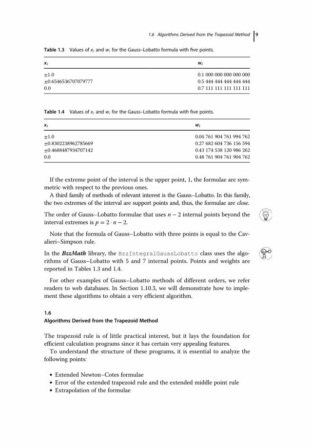
In the BzzMath library, the BzzIntegralGaussLobatto class uses the algo-rithms of Gauss–Lobatto with 5 and 7 internal points. Points and weights arereported in Tables 1.3 and 1.4.

For other examples of Gauss–Lobatto methods of different orders, we referreaders to web databases. In Section 1.10.3, we will demonstrate how to imple-ment these algorithms to obtain a very efficient algorithm.

1.6Algorithms Derived from the Trapezoid Method

The trapezoid rule is of little practical interest, but it lays the foundation forefficient calculation programs since it has certain very appealing features.To understand the structure of these programs, it is essential to analyze the

following points:

� Extended Newton–Cotes formulae� Error of the extended trapezoid rule and the extended middle point rule� Extrapolation of the formulae

Table 1.3 Values of xi and wi for the Gauss–Lobatto formula with five points.

xi wi

�1:0 0.1 000 000 000 000 000�0:6546536707079777 0.5 444 444 444 444 4440:0 0.7 111 111 111 111 111

Table 1.4 Values of xi and wi for the Gauss–Lobatto formula with five points.

xi wi

�1:0 0.04 761 904 761 994 762�0:8302238962785669 0.27 682 604 736 156 594�0:4688487934707142 0.43 174 538 120 986 2620.0 0.48 761 904 761 904 762

1.6 Algorithms Derived from the Trapezoid Method 9

1.6.1

Extended Newton–Cotes Formulae

If a close Newton–Cotes formula is iteratively applied to adjacent intervals, theextended Newton–Cotes formulae are obtained and they exploit the pointsshared by the adjacent intervals.In the case of the trapezoid rule, we have

∫xn

x1

f x� �dx � Th � O b � a� �h2f 2� � (1.32)

with

Th � hf 12� f 2 � f 3 � ∙ ∙ ∙ � f n

2

� �(1.33)

It is worth remarking that the error of the extended formula is O h2� �

since it isequal to the sum of local errors (O h3

� �each) within the single intervals.

The extended Cavalieri–Simpson formula is obtained in an analogous way:

∫xn

x1

f x� �dx � Sh � O b � a� �h4f 5� � (1.34)

with

Sh � h3

f 1 � 4f 2 � 2f 3 � 4f 4 � ∙ ∙ ∙ � 2f n�2 � 4f n�1 � f n� �

(1.35)

Finally, the extended central point:

∫xn

x1

f x� �dx � Mh � O b � a� �h2f 2� � (1.36)

with

Mh � h f 1�1=2 � f 2�1=2 � f 3�1=2 � ∙ ∙ ∙ � f n�1=2h i

(1.37)

and

xi�1=2 � a � i � 12

� �h (1.38)

is the central point of the interval between xi and xi�1 with width h.There are certain features that make the extended trapezoid rule particularly

interesting.

The first important feature of the trapezoid formula is that if we double the inte-gration points (i.e., if we change from an integration step h to h=2), the previouspoints can be used without any recalculation.

For example, let us consider the interval a � 0; b � 4� �. If we adopt theextended trapezoid method for integration with step h � 2, the points we use


are x1 � 0, x2 � 2, and x3 � 4. If we halve the integration step (h � 1), the func-tion must be evaluated in x1 � 0, x2 � 1, x3 � 2, x4 � 3, and x5 � 4. Thus, theprevious function calculations in correspondence with x1; x3; x5 can be exploited.

Note that the points needed with the extended trapezoid formula when the inte-gration step is halved correspond to the points needed by the central point for-mula and the previous integration step.

In the example above, the new points x2 � 1 and x4 � 3 are needed to integratethe function through the extended central point and an integration step h � 2.

Certain programs, which implement the extended trapezoid formula, exploit theproperty:

Th=2 � Th �Mh

2(1.39)

For example, the integral

∫2

1x2 � 1

x

� �dx � 3:026481

We obtain

h � 1 T � 3:25 M � 2:916667h � 0:5 T � 3:08333 M � 2:998214h � 0:25 T � 3:040774 M � 3:019345h � 0:125 T � 3:030059 M � 3:024692h � 0:0625 T � 3:027375 M � 3:026033h � 0:03125 T � 3:026704 M � 3:026368h � 0:015625 T � 3:026536 M � 3:026453h � 0:0078125 T � 3:026495 M � 3:026473h � 0:00390625 T � 3:026484

Note that the convergence speed of the extended trapezoid rule is quite slow.Thus, the method has to be used in this form only when the integral does notrequire a massive computation effort.

1.6.2Error in the Extended Formulae

A second useful feature in the extended trapezoid rule is in the special form ofits local error.

In fact, the error is given by the Euler–MacLaurin relation:

Th � ∫b

af x� �dx �X∞

k�1B2kh

2k

2k� �! f 2k�1� �b � f 2k�1� �ah i

(1.40)

where the coefficients B2k are the Bernoulli numbers.


For many problems, the relation (1.40) can be written in the form

Th � ∫b

af x� �dx �XN

k�1Ckh

2k � RN�1 h� � (1.41)

in which coefficients Ck are independent from h and RN�1 ! 0 with O h2N�2� �.

This relation means that in many practical cases, the extended trapezoid formulahas an error that depends on the even powers of h only.

An analogous relation is also valid for the extended central point method andit is possible in many practical cases to write

Mh � ∫b

af x� �dx �XN

k�1Dkh

2k � QN�1 h� � (1.42)

It is therefore possible to combine the two methods to have an estimation of theerror. This point will be demonstrated later in the chapter.

1.6.3

Extrapolation of the Extended Formulae

The relations (1.41) and (1.42) allow extrapolation techniques to be used. Onlythe relevant steps are reported hereinafter for the extrapolation technique; werefer readers to Vol. 2 (Buzzi-Ferraris and Manenti, 2010b) for detaileddescription:

1) Error estimation. By indicating with Th and T2h two applications of theextended trapezoid rule with integration steps h and 2h, respectively, theerror with step h is estimated:

Ch2 � Th � T2h

3(1.43)

Such an estimation is good if

Th � T2h

Th=2 � Th≅ 4 (1.44)

2) Improving the integral calculation. Once the error is estimated, it can beused to improve the integral estimation:

T*h � Th � Th � T2h

3

� h3

f 1 � 4f 2 � 2f 3 � 4f 4 � ∙ ∙ ∙ � 2f n�2 � 4f n�1 � f n� � � Sh

(1.45)

Note that (1.45) coincides with (1.35) of the extended Cavalieri–Simpsonmethod.


For example, the previous integration results in

h � 1 T � 3:25h � 0:5 T � 3:08333 Ch2 � �5; 55 ? 10�2 T* � 3:027778h � 0:25 T � 3:040774 Ch2 � �1:42 ? 10�2 T* � 3:026587h � 0:125 T � 3:030059 Ch2 � �3:57 ? 10�3 T* � 3:026488h � 0:0625 T � 3:027375 Ch2 � �8:95 ? 10�4 T* � 3:026481

3) Extrapolation. Once T*h have been evaluated, we can estimate

C2h4 � T*

h � T*2h

15(1.46)

and improve the estimation of T*h:

T**h � T*

h � T*h � T*

2h

15(1.47)

For example, the previous integration results in

h � 1 T � 3:25h � 0:5 T � 3:08333 T * � 3:027778h � 0:25 T � 3:040774 T* � 3:026587 T** � 3:026508h � 0:125 T � 3:030059 T* � 3:026488 T** � 3:026481

The procedure can be iterated to calculate the next terms in the Ch6 seriesand so on and, therefore, to further improve the solution. By doing so, theRichardson extrapolation formulae are obtained and they are referred to as theRomberg method in the special case of definite integrals.

The values of Th and the corresponding h can be considered as support pointsof a polynomial interpolation. From this perspective, the Richardson extrapola-tion corresponds to the polynomial prediction for h � 0.

Since the formula for the error of the extended trapezoid formula shows that theterms depend on the even powers of h, it is opportune to use h2 as the indepen-dent variable for the interpolation.

It is possible to demonstrate that the series of predictions obtained with the Rom-berg method coincide with the predictions of the Neville method (Vol. 2, Buzzi-Ferraris and Manenti, 2010b) adapted to the case of z � 0; the polynomial as afunction of h2 and the next points are obtained by continuously halving the step.The column Tk*

h is obtained from the aforementioned T k�1� �*h as follows:

Tk*h � T k�1� �*

h � T k�1� �*h � T k�1� �*

2h

4k* � 1(1.48)

For example, the column T ***h is obtained as follows:

T***h � T**

h � T**h � T**

2h

63


A large number of terms (a large number of columns) should not be used since,at a certain point, the round-off errors caused by the differences between twosimilar numbers introduce numerical instabilities and worsen the results.

The first column obtained with the Romberg method coincides with the oneobtained with the Cavalieri–Simpson method. The other columns can be differ-ent with respect to the ones that we can obtain using the close Newton–Cotesformulae. In particular, the formulae with many Th are different from the high-order Newton–Cotes and this provides a valid motive for the extrapolation withmore elements.

The Romberg method is much more efficient than the extended trapezoid rulemethod, but it is unsuitable in its original version since it is less efficient thanother alternatives.

A newer version that exploits the extrapolation was provided by Stoer andBulirsch (1983). The two main modifications are as follows:

1) The extrapolation is performed using a rational function rather than apolynomial (Bulirsch–Stoer method rather than Neville).

2) The series of Th is not obtained by iteratively halving the integration step.In fact, if the convergence is slow, the series leads to a very small step andlarge number of computations. Stoer and Bulirsch (1983) proposed using adoubled series: the first starts with h=2 and the second with h=3. The ele-ments of the two series are obtained by alternatively halving the previousstep, resulting in h=2, h=3, h=4, h=6, h=8, h=12, h=16, h=24, . . . .

In spite of the modifications introduced by Bulirsch and Stoer, the methodderived from the extended trapezoid rule suffers from several shortcomings thatmake it less efficient than other methods described later, when implemented in ageneral integration program.

Since the trapezoid rule is based on a close formula, functions that cannot beevaluated at the interval extremes cannot be integrated.

For example, it is not possible to calculate the following integral using a closeformula:

I � ∫1

0log x� �dx

Until now, we have assumed that the integration procedure was applied to theoverall initial interval.

Methods that select the integration steps along the initial interval are calledautomatic methods.

If the function to be integrated presents certain zones where integration isharder, the integration step is shortened everywhere, even where the integration


is easier. In other words, this version is not so flexible in accounting for certainlocal needs of the function.

For example, the integral function

I � ∫1

0

ffiffiffix

pdx

has a derivative discontinuity in x � 0. In the neighborhood of such a point, avery small integration step is required to have a certain precision, whereas largerstep can be used elsewhere.For this reason, recent integration programs split the initial interval into a set

of subintervals where the integration procedure is effectively applied using cer-tain strategies described later.

The methods that select the integration steps for each subinterval are calledadaptive methods.

1.7Error Control

To assess the soundness of a numerical integration, it is necessary to estimatethe calculation error.

As usual, there is not one completely reliable individual criterion to accomplishthis task. In other words, we will always encounter problems for which a particu-lar control is incorrect.

In a general integration program, it is opportune to adopt more controls ofdifferent natures. Since we may well encounter wrong results, more controlsallow us to check and compare the same results.A simple way to estimate the error with an algorithm based on the extended

Newton–Cotes formulae is to compare the results by doubling the integrationstep.As seen above, if we use the extended trapezoid formula, the error made using

Th can be estimated as follows:

Ch2 � Th � T 2h

3

It is useful to multiply the estimation by a safety coefficient (i.e., 5). If extrap-olation techniques are adopted, it is possible to estimate the error by calculatingthe difference between the predictions obtained with the Bulirsch–Stoer algo-rithm (or Neville, alias the Romberg method) using different support points, andhence different Th.An alternative technique consists of using as the error estimation the differ-

ence between the extrapolation obtained with the extended trapezoid formulaand the one obtained with the extended central point formula.

1.7 Error Control 15

The error estimate must be compared with an acceptable value that, as perother analogous cases, must be a mix of absolute and relative errors. By denotingwith Ij j the integral estimation of the absolute value of the function, with H theoverall width of the interval, and with h the selected integration step, one possi-ble control is

Error estimate � εabshH

� εrel Ij j� � (1.49)

1.8Improper Integrals

An integral can be theoretically calculated, but it might present the followingnumerical difficulties:

1) The function is infinite in an extreme of the interval. For example, theintegral

I � ∫1

0log x� �dx (1.50)

is analytically well defined and its value is �1, but the function is � ∞ inx � 0.

2) Although the function is analytically finite in an extreme of the interval, itcannot be calculated there numerically. For example, the integral

I � ∫1

0

sin x� �x

dx (1.51)

presents numerical problems if we try to calculate it in x � 0, even thoughthe function is 0 in such a point.

3) The function has certain numerical problems within the integration inter-val. For example,

I � ∫1

�1sin x� �x

dx (1.52)

By means of another example, the integral

I � ∫10

�11ffiffiffiffixj jp dx (1.53)

presents numerical problems in x � 0.4) One or both the interval extremes are infinite like the integral

I � ∫∞

0exp �x� �dx (1.54)


All the previous circumstances may potentially lead to several difficulties using ageneral program for integration. Often, however, an opportune transformationof the integral makes its calculation simpler.


I � ∫∞

1

cos 1x

� �x2

dx (1.55)

can be transformed by substituting t � 1=x

I � ∫1

0cos t� �dt (1.56)

The devices useful in these cases are not considered in this book. We refer read-ers to specialist books on this topic.

While in BVP (boundary value problems), it is not easy to establish the inter-nal point (or points) of the integration interval that might present numericalproblems (see Chapter 6), in the case of definite integrals they are knowna priori. It is therefore possible to split the integration interval so as to havenumerical problems only in one or both the extremes of the integration interval.For example, the integral (1.53) can be obtained as follows:

I � ∫0

�11ffiffiffiffixj jp dx � ∫

10

0

1ffiffiffiffixj jp dx (1.57)

From now, we will assume that numerical problems can arise only at theextremes of the integration interval.

1.9Gauss–Kronrod Algorithms

Gauss formulae have certain advantages with respect to Newton–Cotesformulae.

Given n support points, the Gauss algorithms are exact for 2n � 1� �-degree poly-nomials and therefore they are much more precise than the Newton–Cotes algo-rithms. Very often they are also much more accurate.

There are theoretical reasons for this consideration, which have been largelyconfirmed in practice also. The extended trapezoid method is often superior tothe Gauss integration only for the periodical functions that have a period equalto the integration interval.

Gauss formulae are open. They can be used even when the function has numeri-cal problems at the interval extremes.

1.9 Gauss–Kronrod Algorithms 17


I � ∫1

0log�x�dx

cannot be calculated using a close form even though it is well definite.

Whereas the Newton–Cotes formulae become less efficient as the orderincreases and thus are rarely used beyond the Boole formula, the Gauss formulaebecome increasingly efficient for almost every problem.

Gauss formulae too have certain shortcomings.

If it is necessary to increase the number of points to improve the calculationaccuracy, the previous points are useless.

This problem derives from the fact that orthogonal polynomials (which Gaussformulae are based on) have distinct zeroes for different polynomial orders.Since the points where the function must be calculated are the zeroes of anorthogonal polynomial, they are different in every formula from the same family(except for the central point).A direct consequence of this fact is the difficulty in estimating the error using

a specific Gauss formula.

If we want to control a Gauss formula with a formula with a higher order, it isnecessary to calculate the function in all the points of the two formulae (some-times with the exception of the central point).

As already mentioned, it is useful to use the weight r x� � in an optimal way soas to exploit the Gauss formulae to the fullest: the remaining portion of thefunction should be well representable by a polynomial.

In the following, we only describe the Gauss–Legendre methods (with r x� � � 1and extremes �1 and 1).

The Russian mathematician Kronrod brilliantly solved the problem of errorestimation in the Gauss–Legendre formulae. He found a family of formulaebased on 2n � 1 points, where n of them are the zeroes of the Legendre polyno-mial (thus, the n points of a Gauss–Legendre formula). Contrary to a Gauss for-mula (which has a precision of 4n � 2 with 2n � 1 points), these formulae have aprecision of 3n � 1, which is enough to control the Gauss formula constituted byn points and with precision of 2n.Given 2n � 1 points of the Kronrod formula, two approximations of the inte-

gral can be calculated:

� The first exploits wi and xi of the Gauss formula:

Gn �Xni�1

wi f i (1.58)


� The second exploits, beyond the previous n points xi, n � 1 new points anduses opportune weights vi ≠ wi:

K 2n�1 �X2n�1i�1

vi f i (1.59)

The couple of formulae commonly used consist of the Gauss formula with 7points together with the Kronrod one with 15 points (see Tables 1.5 and 1.6).The difference between K 2n�1 and Gn can be used as estimate of the error

using K 2n�1 for the integral calculation.Some authors (Kahaner, Moler, and Nash, 1989) think that this estimate is too

pessimistic and, based on practical experience rather than on theoretical reasons,they suggest to use

Error estimate � 200Gn � K2n�1j j� �1:5 (1.60)

1.10Adaptive Methods

The adaptive methods concentrate computational effort in the subintervals thatpresent the largest difficulties for numerical integration. They differ from theautomatic methods in that they do not evenly split the interval.

Table 1.5 Values of xi and wi for the Gauss formula with seven points.

xi wi

�0:949107912342759 0.129 484 966 168 870�0:741531185599394 0.279 705 391 489 277�0:405845151377397 0.381 830 050 505 1190.0 0.417 959 183 673 469

Table 1.6 Values of xi and vi for the Kronrod formula with 15 points to control the Gaussformula with 7 points.

xi wi

�0:991455371120813 0.022 935 322 010 529�0:949107912342759 0.063 092 092 629 979�0:864864423359769 0.104 790 010 322 250�0:741531185599394 0.140 653 259 715 525�0:586087235467691 0.169 004 726 639 267�0:405845151377397 0.190 350 578 064 785�0:207784955007898 0.204 432 940 075 2980.0 0.209 482 141 084 728

1.10 Adaptive Methods 19

The seminal idea is trivial: the function is integrated within a generic interval. Iferror control is satisfactory, the portion of the integral is added to the global inte-gral; otherwise, the interval is split into two subintervals (usually, but not necessar-ily, of the same width) and the same procedure is recursively invoked twice.

The adaptive methods are particularly easy to implement in programming lan-guages, such as C/C++, that accept recursive functions.

1.10.1

Method Derived from the Gauss–Kronrod Algorithm

The implementation of this algorithm to make it adaptive is conceptually simple.The Kronrod formula with 15 points is adopted as basis. We start to calculate

the integral on the overall integration interval. If the error controlled by (1.60) isgood, the integral value is returned; otherwise, the interval is halved and theKronrod formula is adopted for both the subintervals.The resulting program is very high performance and constitutes the founda-

tion of many programs for the adaptive integration.

In the BzzMath library, the BzzIntegralGauss class adopts this philosophy.

In some circumstances, the function cannot be represented properly with apolynomial in the neighborhood of an extreme of the interval. Consider the fol-lowing integrals:

I � ∫1

0

ffiffiffix

pdx (1.61)

I � ∫1

0

1ffiffiffix

p dx (1.62)

I � ∫1

0

1x0:8

dx (1.63)

In each, the integral function cannot be represented by a polynomial in x � 0.

In these cases, the Gauss idea that allows the exact integration of a2n � 1� �-degree polynomial given n support points in the subinterval near to 0 isno longer appealing. On the other hand, it could be advantageous to find an � 1� �-degree polynomial that best represents the function in such an interval.This polynomial can be obtained by using the roots of the Chebyshev polynomial(see Vol. 2, Buzzi-Ferraris and Manenti, 2010b) as support points.

It may be opportune to split the integral into three distinct integrals:

I � ∫a�da

af x� �dx � ∫

b�db

a�daf x� �dx � ∫

b

b�dbf x� �dx (1.64)


The intermediate integral

I2 � ∫b�db

a�daf x� �dx (1.65)

is calculated with the aforementioned Gauss–Kronrod algorithm. The remainingtwo integrals are performed on very small intervals using the Chebyshev supportpoints rather than the Gauss ones.

In the BzzMath library, the BzzIntegralGaussBF class carries out the inte-gration using this philosophy.

1.10.2

Method Derived from the Extended Trapezoid Algorithm

In the automatic methods based on the extended trapezoid formula, overall inte-gration interval is considered: if the error is dissatisfactory, new points uniformlydistributed on the interval are inserted.To make the procedure adaptive, the same technique on parts of the interval

may be used, so as to make the calculations denser in correspondence withregions posing certain difficulties.

To develop an efficient adaptive method based on the extended trapezoidmethod, we can change perspective.

It is preferable to develop a class that uses a predefined number of points andto use the objects of this class in a recursive way.

If the object is based on 13 points (extremes included), the subinterval is splitinto 12 evenly spaced intervals. Note that we select 12 intervals since 12 is divisi-ble by 1, 2, 3, 4, 6, and 12.

It is therefore possible to use 13 points to calculate a series of six integralswith the extended trapezoid method (with 2, 3, 4, 5, 7, and 13 points) and aseries of four integrals with the extended central point method (with 1, 2, 3, and6 points). It is possible to extrapolate both the series to zero with the Bulirsch–Stoer algorithm and also to compare the two results to have an estimate of theerror.

The advantage to considering the 13 points as simultaneously present is that wecan exploit a series of six calculations of the extended trapezoid formula onwhich to perform the extrapolation.

To have the same number of elements with the Romberg method, we need 33function calculations (extremes included). If we use the Bulirsch series, the num-ber of points is, again, 13, but the more precise integral is obtained with steph=8, with respect to h=12 using this algorithm.If the error is unsatisfactory, the interval is split into two parts and the proce-

dure is iterated on both the new subintervals.

1.10 Adaptive Methods 21

Note that both the subintervals already have seven values of the function placedat the desired position so as to be ready to iterate the procedure and, therefore,they need only six new points each.

In this implementation, it is crucial to be able to dynamically manage memoryallocation. In fact, each subinterval can be further split and, every time this isdone, a space has to be created to collect the function values in the six newpoints required by the procedure. When the error is good on a portion of theinterval, all the memory allocated for that portion is no longer necessary andcan be promptly freed up and made available.Since the extremes can be nonevaluable, the initial interval is split into three

subintervals. The two external subintervals are very small and are solved usingthe Gauss–Kronrod method.

In the BzzMath library, the BzzIntegral class adopts this philosophy.

1.10.3

Method Derived from the Gauss–Lobatto Algorithm

The adaptive methods that use the Gauss–Lobatto algorithms have the followingpros and cons.

Positive Aspect

1) Using the Gauss–Lobatto algorithms with an odd number of supportpoints (i.e., five and seven points), three points are common to the algo-rithms. Therefore, nine points are needed at the first iteration with the twoalgorithms with five and seven points.

2) In the successive iterations, two of the previous points (the extreme pointsof the algorithms) can be reused. Thus, in this case, only seven points arenecessary.

Since the Gauss–Lobatto rules are based on a close formula, functions that can-not be evaluated at the interval extremes cannot be integrated.

To overcome this problem, the same technique used with the extended trape-zoid method implemented in the class BzzIntegral can be adopted: split theoriginal interval into three subintervals where the external ones are very small.The objects of the BzzIntegralGaussBF class use this device too, but for dif-ferent reasons. In the first case, it is necessary because the extended trapezoidformulae are close, whereas in the second case, the polynomial approximationcan be improved in these delicate intervals.

In the BzzMath library, the BzzIntegralGaussLobatto class adopts a differ-ent strategy to the ones used to solve the same problem with the classes BzzIn-

tegral and BzzIntegralGaussBF.

In this class, the two lateral intervals are much smaller and, rather than using apolynomial approximation of the integral function, the following approximation


is adopted:

f x� � � αxβ (1.66)

The two parameters are evaluated by means of an exact interpolation usingtwo points inside the interval. The two selected points are obtained with thethree-point Radau algorithm. The approximating integral is calculated analyti-cally. This procedure is used only if the function in the three points (two internaland one extreme of the interval) is increasing or decreasing. The three-pointRadau formula is adopted otherwise.

1.11Parallel Computations

All the adaptive methods already discussed can be parallelized. In fact, in eachsubinterval, we can simultaneously calculate the values of the integral functionrequired by the algorithm.

In the BzzMath library, all the classes for the calculation of definite integralsautomatically exploit the openMP directives when the compiler allows it.

1.12Classes for Definite Integrals

The following classes dedicated to the calculation of definite integrals

I � ∫b

af x� �dx (1.67)

are implemented in the BzzMath library:

� BzzIntegralGauss: Based on the Gauss–Kronrod formulae.� BzzIntegralGaussBF: The interval is split into three subintervals. Thelateral subintervals are very small and an interpolating polynomial based onChebyshev points is adopted. The central interval is solved using theGauss–Kronrod formulae.� BzzIntegral: The interval is split into three subintervals. The lateral sub-intervals are very small and the Gauss–Kronrod formulae are used. Theextended trapezoid formulae based on the extrapolation with 13 points areadopted for the central subinterval.� BzzIntegralGaussLobatto: The interval is split into three subintervals.The lateral subintervals are very small and the interpolation (1.66) isadopted with increasing or decreasing functions; the three-point Radau for-mula is adopted otherwise. The central subinterval uses the Gauss–Lobattowith five and seven points.

1.12 Classes for Definite Integrals 23

The classes

BzzIntegralGauss

BzzIntegral

are often more accurate and efficient for common problems. On the other hand,the classes

BzzIntegralGaussBFBzzIntegralGaussLobatto

perform better in the case of functions with problems at the interval extremes.

All these classes have a constructor that requires the name of the function thatwe have to integrate as their argument:

BzzIntegral i12(IntFun);BzzIntegralGauss iG(IntFun);BzzIntegralGaussBF iBF(IntFun);BzzIntegralGaussLobatto iLo(IntFun);

The integral function must be defined in a code function, which has thegeneric value of t as its argument and the value of the integral function calcu-lated in t as return. For example,

double IntFun(double t){return sqrt(t);}

Once an object of one of the classes has been defined, it can be used throughthe overlapped operator (), which requires as the argument the extremes of thedesired interval and has as return the calculated integral for such an interval.For example:

BzzIntegral i(IntFun);double I = i(0.,10.);

Example 1.1

Calculate the integral:

I � ∫1

0

1ffiffit

p dt � 2

The program is


//prototypedouble IntegralProblem(double t);


void main(void){BzzIntegral i(IntegralProblem);double I = i(0.,1.);BzzIntegralGauss iG(IntegralProblem);double IG = iG(0.,1.);BzzIntegralGaussBF iGBF(IntegralProblem);double IGBF = iGBF(0.,1.);

BzzIntegralGaussLobatto iLob(IntegralProblem);double ILOB = iLob(0.,1.);

BzzPrint(“\nCorrect Value %22.14e”,2.);BzzPrint(“\nBzzIntegral %22.14e”,I);BzzPrint(“\nBzzIntegralGauss %22.14e”,IG);BzzPrint(“\nBzzIntegralGaussBF %22.14e”,IGBF);BzzPrint(“\nBzzIntegralLobatto %22.14e”,ILOB);

}double IntegralProblem(double t)

{return 1. / sqrt(t);}

The objects of all the classes automatically receive a default value for the abso-lute error, the relative error, the minimum integration step, and the maximumnumber of iterations after which the calculations are stopped.If we wish to modify certain values of these parameters, we can use the follow-

ing functions:

i.SetTolAbs(tolA);i.SetTolRel(tolR);i.SetMinH(hm);i.SetMaxFunctions(numMax);

Example 1.2

Calculate the integral:

I � ∫∞

0

tet � 1

dt � π2

6

Since an extreme is infinite, it is necessary to use an iterative procedure. Webegin by calculating the integral between 0 and an assigned value. Next, we cal-culate another integral and add it to the previous one; this new integral uses theprevious upper extreme as the lower extreme. The procedure is iterated until thevalue added to the overall integral is negligible.The kernel of the program can be implemented as follows:

tI = 0.; tF = 5.; delta = 5.;I = i(tI,tF);

1.12 Classes for Definite Integrals 25

do{tI = tF; delta *= 2.; tF += delta;II = i(tI,tF);I += II;} while(fabs(II) > fabs(0.00001*I));

Additional examples and tests of the use of

BzzIntegral,BzzIntegralGauss,BzzIntegralGaussBF,

and

BzzIntegralLobatto

classes can be found in

BzzMath/Examples/BzzMathAdvanced/DefiniteIntegral

directory and

IntegralIntegralTests

subdirectories in BzzMath7.zip file available at the web site:www.chem.polimi.it/homes/gbuzzi.

1.13Case Study: Optimal Adiabatic Bed Reactors for Sulfur Dioxide with Cold Shot Cooling

Lee and Aris (1963) solved the problem of the optimal design of a multibed adia-batic converter using dynamic programming. Specifically, they selected the caseof sulfur dioxide oxidation.The problem was to design a reactor with N adiabatic beds and, for the sake of

definitiveness, N � 3, as reported in Figure 1.1.The reactant stream of total mass flow G is split into two parts: one fraction

λ3G going to a preheater, where the temperature is raised to T3, and the remain-ing part 1 � λ3� �G serving as a bypass cooling stream. The composition is definedby the conversion g, and within each reactor the conversion passes from gi to g i,thanks to the catalyst. Also, the temperature adiabatically goes from Ti to T i forthe overall exothermicity of the reaction mechanisms within each reactor. Thus,it is necessary to refrigerate the stream between two adjacent stages.The link between the normalized T, t, and the conversion across each adia-

batic stage is considered linear:

t � g � tn � gn� �

(1.68)



The reactor system design needs to be optimized to improve the overall profit-ability of the process.

F � λ3 g 3 � g3 � δ ?ϑ3� � � λ2 g 2 � g2 � δ ? ϑ2

� �� g 1 � g1 � δ ? ϑ1� � � μ ? λ3 ? t3

(1.69)

where δ � 0:03125, μ � 0:15, and ϑn is the residence time in the nth bed:

ϑn � ∫gn´

gn

dgRn g; t�g�� (1.70)

The chemical reaction is

SO2 � 12O2 $ SO3 (1.71)

Calderbank’s kinetic expression (1953) is of the form

r � k1ffiffiffiffiffiffiffiffiffipSO2

ppO2

� k2

ffiffiffiffiffiffiffiffiffipO2

pSO2

spSO3

(1.72)

If these values are used, the result is

R g; t� � � 3:6 � 106 exp 12:07 � 501 � 0:311t

� � ffiffiffiffiffiffiffiffiffiffiffiffiffiffi2:5 � g

p3:46 � 0:5g� �

32:01 � 0:5g� �1:5"

�exp 22:75 � 86:451 � 0:311t

� �gffiffiffiffiffiffiffiffiffiffiffiffiffiffiffiffiffiffiffiffiffiffiffi3:46 � 0:5g

p32:01 � 0:5g� � ffiffiffiffiffiffiffiffiffiffiffiffiffiffi

2:5 � gp

#

(1.73)

The problem consists of finding the values of g 1, g 2 , g 3, λ2, λ3, t3 that maximizethe objective function (1.69). Optimization is difficult since g 1, g 2, g 3 cannotbe selected arbitrarily, but have to be such that the corresponding point on theadiabatic curve, which starts from the inlet values of each stage, does not over-come the equilibrium curve. Conversely, it is not possible to perform the inte-gration (1.70).

3 2 1

(1−λ3)G (1−λ2)G

Mass flow GG

Conversion

Temperature

λ3G λ2Gg0 g3 g2g3′ g2′ g1′

T3′ T2

′ T1′

g1

T0 T3 T2 T1

Figure 1.1 Reactor system.

1.13 Case Study: Optimal Adiabatic Bed Reactors for Sulfur Dioxide with Cold Shot Cooling 27

The BzzMinimizationRobust class allows the infeasible points to be dis-carded quite simply.

The integrals (1.70) are calculated using the BzzIntegralGauss class.

Example 1.3

Optimize the reactor design of the Lee and Aris (1963) system. The program is

#define BZZ_COMPILER 0#include “BzzMath.hpp”double tt,gg;int SO2Equilibrium(double ttt,double ggg,double g);double SO2Integral(double g);double SO2(BzzVector &x);void main(void)

{BzzVector x0(6,2.1,2.,1.5,0.5,0.2,4.);BzzVector xMin(6),xMax(6,2.465,2.465,

2.465,1.,1.,100.);BzzMinimizationRobust m(x0,SO2, &xMin, &xMax);double start = BzzClock();m();BzzPrint(“\nSeconds: %e”,

BzzClock() - start);m.BzzPrint(“Results”);BzzPause();}

int SO2Equilibrium(double ttt,double ggg,double g){if(g > 2.5)

return 1;double t = g + (ttt - ggg);double k1 = exp(12.07 - 50. / (1. + 0.311 * t));double k2 = exp(22.75 - 86.45

/ (1. + 0.311 * t));double c1 = sqrt(2.5 - g) * (3.46 - 0.5 * g)

/ pow(32.01 - 0.5 * g,1.5);double c2 = g * sqrt(3.46 - 0.5 * g) /

((32.01 - 0.5 * g) * sqrt(2.5 - g));if(k1 * c1 > k2 * c2)

return 1;else

return 0;}


double SO2Integral(double g){double R;double t = g + (tt - gg);double k1 = exp(12.07 - 50. / (1. + 0.311 * t));double k2 = exp(22.75 - 86.45

/ (1. + 0.311 * t));double c1 = sqrt(2.5 - g) * (3.46 - 0.5 * g)

/ pow(32.01 - 0.5 * g,1.5);double c2 = g * sqrt(3.46 - 0.5 * g) /

((32.01 - 0.5 * g) * sqrt(2.5 - g));R = 3.6e6 * (k1 * c1 - k2 * c2);return 1. / R;}

double SO2(BzzVector &x){int okEq;double gp1 = x[1];double gp2 = x[2];double gp3 = x[3];double l2 = x[4];double l3 = x[5];double t3 = x[6];double G = 50.;double mu = 0.15;double delta = 0.03125;double g3 = 0.;//l3 * G;double g2 = l3 * gp3 / l2;double g1 = l2 * gp2;double tp3 = gp3 + (t3 - g3);double t2 = l3 * tp3 / l2;double tp2 = gp2 + (t2 - g2);double t1 = l2 * tp2;double tp1 = gp1 + (t1 - g1);if(SO2Equilibrium(t1,g1,gp1) == 0 ||

SO2Equilibrium(t2,g2,gp2) == 0 ||SO2Equilibrium(t3,g3,gp3) == 0)

{bzzUnfeasible = 1;return 0.;}

BzzIntegralGauss iG(SO2Integral);tt = t1; gg = g1;double theta1 = iG(g1,gp1);tt = t2; gg = g2;

1.13 Case Study: Optimal Adiabatic Bed Reactors for Sulfur Dioxide with Cold Shot Cooling 29

double theta2 = iG(g2,gp2);tt = t3; gg = g3;double theta3 = iG(g3,gp3);double f = l3 * (gp3 - g3 - delta * theta3)

+ l2 * (gp2 - g2 - delta * theta2)+ (gp1 - g1 - delta * theta1)- mu * l3 * t3;

return -f;}

The results are

xStart1 2.20000000000000e+0002 2.10000000000000e+0003 1.50000000000000e+0004 6.00000000000000e-0015 3.00000000000000e-0016 4.00000000000000e+000Function Value -4.73705038799949e-001

xSolution1 2.45025718587293e+0002 2.37391222293976e+0003 2.04237012795229e+0004 7.59477671271243e-0015 4.88125377107788e-0016 3.45269557794849e+000Function BzzMinimum Value -2.12180401518867e+000

Please note that in the original paper, there was an error in the use of thedynamic programming, highlighted in Malengé and Villermaux (1967). The opti-mal values calculated in these works were 2.036 and 2.107 and thus smaller thanthe 2.1218 result obtained here.


2Ordinary Differential Equations Systems


2.1Introduction

This chapter deals with the numerical integration of systems of ordinary differ-ential equations of the first order and in the explicit form:

y´ � f y; t� � (2.1)

with the initial conditions:

y t0� � � y0 (2.2)

An ordinary differential equations system is indicated with the acronym ODE.

For example, the design of a refrigerated plug flow reactor is governed by threedifferential equations:

dxdw

� f 1 x;T ;P� �dTdw

� f 2 x;T ;P� �dPdw

� f 3 x;T ;P� �with the initial conditions w � 0; x � 0;T � T 0;P � P0, which allow us to calcu-late the conversion x, the temperature T , and the pressure P as functions of theresidence time w.Any differential equation with higher order m in the form

y m� � � f y; y 1� �; . . . ; y m�1� �; t� �

(2.3)

31



with the initial conditions

y t0� � � y0

y 1� � t0� � � y 1� �0

..

.

y m�1� � t0� � � y m�1� �0

(2.4)

can be transformed into a system (2.1) through the introduction of new depen-dent variables.For example, the third-order equation:

y´´´ � ty´´ � y´ � 1 � t � y� �2 � sin t� �y´´ 0� � � 1; y´ 0� � � 2; y 0� � � 3

is transformed into the system:

y1 � y2

y2 � y3

y3 � ty3 � y2 � 1 � t � y1� �2 � sin t� �

with the conditions:

y3 0� � � 1

y2 0� � � 2

y1 0� � � 3

thanks to the introduction of the variables:

y1 � y

y2 � y´ � y1y3 � y´´ � y2

Numerical programs for the solution of differential equations usually ask theuser for the manual transformation of an equation with high-order derivativesinto a system in the form (2.1).

A small advantage arising from the problem transformation is the fact that thenumerical value of the derivatives is achieved without any computational effortbeing expended, since they are to the same as the dependent variables insertedduring the transformation itself.

The following problems are not considered in this chapter.

1) Ordinary differential equation systems with boundary conditions (seeChapter 6).

2) Differential–algebraic equations (DAE) systems (see Chapter 4).3) Partial differential equations (PDE) systems.

32 2 Ordinary Differential Equations Systems

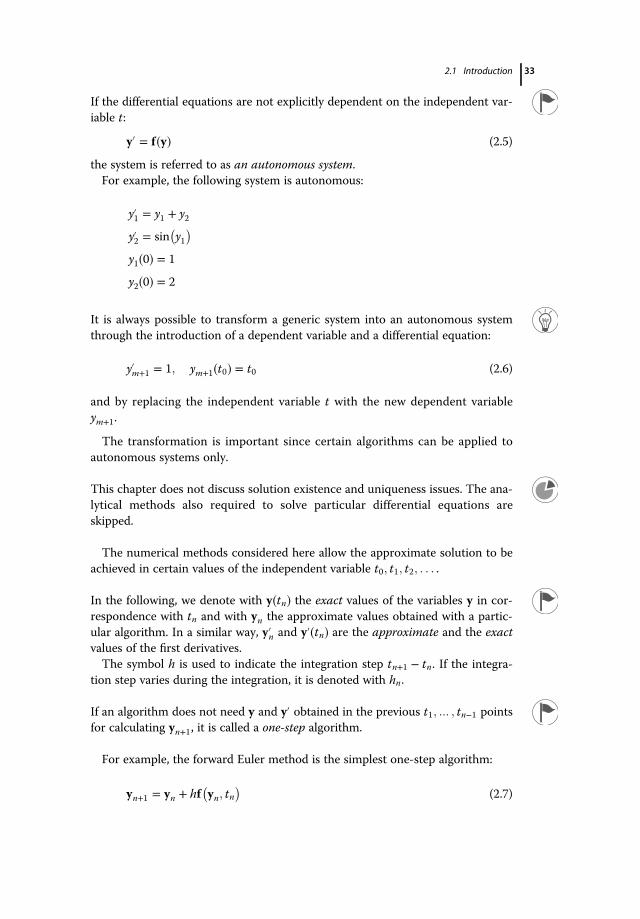
If the differential equations are not explicitly dependent on the independent var-iable t:

y´ � f y� � (2.5)

the system is referred to as an autonomous system.For example, the following system is autonomous:

y1 � y1 � y2

y2 � sin y1� �

y1 0� � � 1

y2 0� � � 2

It is always possible to transform a generic system into an autonomous systemthrough the introduction of a dependent variable and a differential equation:

ym�1 � 1; ym�1 t0� � � t0 (2.6)

and by replacing the independent variable t with the new dependent variableym�1.

The transformation is important since certain algorithms can be applied toautonomous systems only.

This chapter does not discuss solution existence and uniqueness issues. The ana-lytical methods also required to solve particular differential equations areskipped.

The numerical methods considered here allow the approximate solution to beachieved in certain values of the independent variable t0; t1; t2; . . . .

In the following, we denote with y tn� � the exact values of the variables y in cor-respondence with tn and with yn the approximate values obtained with a partic-ular algorithm. In a similar way, yn and y´ tn� � are the approximate and the exactvalues of the first derivatives.The symbol h is used to indicate the integration step tn�1 � tn. If the integra-

tion step varies during the integration, it is denoted with hn.

If an algorithm does not need y and y´ obtained in the previous t1; ::: ; tn�1 pointsfor calculating yn�1, it is called a one-step algorithm.

For example, the forward Euler method is the simplest one-step algorithm:

yn�1 � yn � hf yn; tn� �

(2.7)

2.1 Introduction 33

A multistep algorithm uses y or/and y´ obtained in the previous pointst1; . . . ; tn�1 to calculate yn�1.

An example of multistep method is

yn�1 � yn�1 � 2hf yn; tn� �

(2.8)

A method that does not need any evaluation of f in yn�1; tn�1 is called an explicitmethod.

For example, the second-order Runge–Kutta algorithm is explicit:

k1 � hf yn; tn� �

(2.9)

k2 � hf yn � k1; tn � h� �

(2.10)

yn�1 � yn � k1 � k22

(2.11)

Any method that needs the evaluation of f in yn�1; tn�1 is called an implicitmethod.

The backward Euler algorithm is implicit:

yn�1 � yn � hf yn�1; tn�1� �

(2.12)

If f are nonlinear, as is usually the case, the implicit methods require the solu-tion of a nonlinear system. Thus, they are significantly heavier than the explicitmethods in terms of both the implementation and computational efforts.

In the following, we will demonstrate that implicit methods are more stable andallow the use of larger h than explicit methods.

A large number of algorithms for the integration of differential equations withinitial conditions have been proposed. They can be classified in several differentways.

1) Based on the number of points tn used in the formula: one-step or multi-step methods.

2) Based on the criterion used to obtain the formula: Taylor series expansionor polynomial approximation methods.

3) According to f dependence with respect to yn�1; tn�1: explicit or implicitmethods.


2.2Algorithm Accuracy

Each algorithm has its own local error, depending on the approximate formula itis based on (see Vol. 1, Buzzi-Ferraris and Manenti, 2010a). The local error iscalculated under the hypothesis of exact data and numerical calculations, as itis connected only to the approximate model.

Knowing how to calculate the local error of a specific algorithm is not impor-tant here. It is enough to remark that it depends on a known power of the inte-gration step. For example, the Runge–Kutta algorithm (2.9)–(2.11) has a localerror of O h3

� �.

The local error can be expressed analytically for many algorithms. For exam-ple, the Euler forward method (2.7) has the local error h2ny

´´ ξn� �=2, which isO h2� �

.

An algorithm is p-order if it exactly integrates an ordinary differential equationhaving a p � 1-degree polynomial as its solution, but it is not able to exactly inte-grate a differential equation having a p-degree polynomial as its solution. Someauthors indicate with p the precision of the algorithm.

For example, the Adam–Bashforth method:

yn�1 � yn � h 3f yn; tn� � � f yn�1; tn�1

� �� 2

(2.13)

is exact if the solution of the differential equation is a 1-degree polynomial, andhence it is a second-order algorithm. The local error is 5h3y�3� ξn� �=12 and O h3

� �.

Be careful not to confuse the order of the algorithm and the order of its localerror.

The fourth-order Runge–Kutta method has local error O h5� �

and it is exact ifthe solution is a third-order polynomial.

Theoretically, algorithms with higher orders have smaller local errors and allowlarger integration steps.

This is true only if the exact solution can be well approximated with a polyno-mial. The approximation usually initially improves with higher orders of p andthen worsens after a certain order (see Vol. 2, Buzzi-Ferraris and Manenti,2010b).

In practice, it is reasonable to select a good compromise between the localerror and the order p: the latter cannot be too small to avoid large local errorsand hence too small integration steps; p cannot be too large to prevent

2.2 Algorithm Accuracy 35

numerical problems. The optimal order p is usually 4 or 5. If the problem to besolved is relatively soft, the order can be larger, whereas it should be smaller forharder problems.

An algorithm is convergent if the accuracy of the solution improves while h ! 0,under the assumption of no round-off errors.

All the methods of practical interest are convergent.

2.3Equation and System Conditioning

As described in our Vol. 1 (Buzzi-Ferraris and Manenti, 2010a), numericallydescribing a real phenomenon, it should not involve explosive or chaotic behav-iors. In other words, it should be characterized by stable conditions. For exam-ple, it is well known that it is not possible to mathematically describe oscillationsof a double pendulum when the oscillations are very wide.

To clarify this concept and avoid any mix-ups with other kinds of instabilityproblems, let us state that when we refer to real physical problems, we will betalking about well-posed and ill-posed problems.

There may be several different ways to model a well-posed physical problemmathematically. Some of these formulations may be sensitive to small perturba-tions, whereas others may not.

In the former case, the mathematical formulation is ill-conditioned; otherwise, itis well conditioned.

Note: Many books on numerical analysis also use the term stability for the con-ditioning of differential equations.

It is important to note that problem formulation is well conditioned or ill-con-ditioned independent of the numerical algorithm. If the physical phenomenon isill-posed or its formulation is ill-conditioned, no numerical methods will be ableto solve it.

An algorithm is stable if it is able to control the increase in the round-off errorwhen the problem is well posed and its formulation is well conditioned.Conversely, the algorithm is unstable when it cannot control the amplification

of the round-off error, although the problem is well posed and its formulation iswell conditioned.

After this brief review, let us consider a single differential equation:

y´ � f y; t� �; y t0� � � y0 (2.14)

to better clarify the important concepts of equation conditioning and algorithmstability and the differences between them.


The equation is well conditioned if a small perturbation in the function f or inthe initial condition y0:

y´ � f y; t� � � δ t� �y t0� � � y0 � ε

(2.15)

generates a solution (obtained without numerical errors) only slightly far fromthe theoretical solution of (2.14).On the other hand, the equation is ill-conditioned when a small perturbation

generates a significant deviation in the solution.Let us consider, for example, the differential equation:

y´ � 9y � 10e�t ; y 0� � � 1

The general solution is

y � e�t � ce9t

Since the initial condition requires c � 0, the analytical solution is

y � e�t

This formulation is ill-conditioned since a small perturbation of the initial con-ditions is enough to obtain a completely different solution. In fact, by modifyingthe initial condition as follows:

y 0� � � 1:0001

the new analytical solution is

y � e�t � 0:0001 � e9tThe two solutions in t � 1 are 0:367879 and 1:178188, respectively

(see Figure 2.1).

0

0.2

0.4

0.6

0.8

1

1.2

1.4

10.80.60.40.20

exp(-t)

exp(-t)+0.0001*exp(9t)

Figure 2.1 Ill-conditioned formulation.

2.3 Equation and System Conditioning 37

The solution of a differential equation consists of a special trend univocallydetermined by the differential equation itself and the initial conditions. Figure 2.2shows an ill-conditioned equation formulation: small perturbations in the initialconditions or small deviations from the solution lead to completely differenttrends.On the other hand, the equation formulation is well conditioned in Figure 2.3,

where all the curves converge to a single solution.

The well conditioning or ill-conditioning depends upon the direction used tointegrate the differential equation: a well-conditioned equation is ill-conditionedin the opposite direction.

In practical problems, many intermediate and extreme situations are possible.For example, it may happen that a differential equation is well conditioned in acertain interval and ill-conditioned in another interval.Please note that we may have different problems with the same solution and

some of them are well conditioned and others ill-conditioned.

Figure 2.2 Ill-conditioned formulation; all the curves diverge.

Figure 2.3 Well-conditioned formulation; all the curves converge to the single solution.


For example, the differential equations

y´ � 9y � 10e�t ; y 0� � � 1

y´ � e�t ; y 0� � � 1

y´ � �y; y 0� � � 1

have the same solution:

y t� � � e�t

By perturbing the initial condition as follows:

y 0� � � 1:0001

we obtain respectively:

y t� � � e�t � 0:0001 � e9ty t� � � e�t � 0:0001

y t� � � e�t � 0:0001 � e�t

The new solution diverges from the previous one in the first case, demon-strates a constant deviation in the second case, and converges to the originalsolution in the last case.

Clearly, the phenomenon cannot be a property of the solution, since this is thesame for all these problems, and must be a property of the differential systemitself. It is therefore appropriate to speak about well conditioning or ill-condition-ing of the system formulation.

The conditioning of a differential equation depends on the family of all possiblesolutions obtained with different initial conditions of the same equation or start-ing from points slightly different from the solution.

Let us consider the differential equation (2.14). The tangent to a curve y t� �, thesolution of the equation in y; t

� �, is y´ � f y; t� �. The variation of the tangent with

y by keeping t constant is given by the derivative f y. In the instance of Figure 2.2,an increase in y leads to a more positive value of the tangent and f y > 0. Con-versely, f y is negative in the situation of Figure 2.3.

To have a well-conditioned equation (2.14), we need f y < 0. Only in this casewill the curves of the family converge to the single solution. When f y > 0, theequation is ill-conditioned and the curves diverge.

For example, the equation y´ � �10y is well conditioned since f y � �10 < 0,whereas the equation y´ � 10y is ill-conditioned for f y � 10 > 0.

2.3 Equation and System Conditioning 39

The conditioning of an ordinary differential equation system:

y´ � f y; t� � (2.16)

is studied through the eigenvalues λ1; λ2; . . . ; λN of its Jacobian J, where

J ij � @f i@yj

(2.17)

Generally speaking, the eigenvalues λ1; λ2; . . . ; λN can be complex numbers. Ifthe real part of an eigenvalue is largely positive, the system is ill-conditioned; ifall the eigenvalues have a negative real part, the system is well conditioned.

2.4Algorithm Stability

To make the reasoning easier to understand, let us consider the Euler algorithmapplied to a single differential equation:

yn�1 � yn � hn � f yn; tn� �

(2.18)

If this relation is subtracted from the Taylor expansion series, it gives

y tn�1� � � yn�1 � y tn� � � yn � hn f y tn� �; tn� � � f yn; tn� �� h2ny

´´ ξn� �2

(2.19)

The difference y tn�1� � � yn�1 represents the global error in tn�1 and this is fortwo reasons:

1) Local error: h2ny´´ ξn� ��

=2. As already-mentioned and in Buzzi-Ferraris andManenti (2010a), the local error is due to the model approximation. It isestimated by assuming that the calculations are performed without numer-ical errors and that the exact required data are known: In this case, weassumed the exact value of y in tn; y tn� �� was known.

2) Propagation error: Since the exact value y tn� � is unknown in tn, we knowonly its approximation yn and thus we have a second source of error inde-pendent of the local error. This error can be estimate by means of thesecants theorem: Given a function Φ x� � and two values Φ xA� � and Φ xB� �obtained in xA and xB, there is a point ζ within the interval xA; xB� � wherethe function’s derivative is equal to the secant obtained with the previouspoints:

Φ xA� � �Φ xB� �xA � xB

� Φ´ ζ� � (2.20)


Thus, it results in

f y tn� �; tn� � � f yn; tn� �

y tn� � � yn� f y z� �; tn < z < tn�1 (2.21)

and therefore

Global Error in tn�1 � 1 � hnf y� �

Global Error in tn � Local Error (2.22)

If

1 � hnf y

�� > 1 (2.23)

the Euler algorithm is unstable since the error increases with the itera-tions. To make the algorithm stable, it is necessary to select an integrationstep hn such that

1 � hnf y

�� < 1 (2.24)

1 � hnf y� �

is the amplification factor κ of the global error for the Euleralgorithm.

It is important to stress that the conditioning of a differential equation (or sys-tem) and the stability of the algorithm used to solve it are different conceptsand the criteria used to analyze them are even different.

An equation is ill-conditioned if

f y > 0 (2.25)

In this case, the Euler algorithm is always unstable when hn > 0.

It is pointless to check the algorithm’s stability when the differential equation isill-conditioned. What is important is to check the stability of the algorithm forwell-conditioned problems.

If the equation is well conditioned, it results in

f y < 0 (2.26)

In this case, the Euler algorithm is stable only if

hn < � 2f y

(2.27)

For example, let us use the Euler method to solve the differential equation:

y´ � �1000y � 1000; y 0� � � 10

2.4 Algorithm Stability 41

The equation is very well conditioned since f y � �1000 and the analytical solu-tion is

y � 1 � 9e�1000t

If we use an integration step h > 0:002, the Euler method becomes unstable. If tis sufficiently large, the solution is y � 1. Since the Euler method is exact for poly-nomials with degrees smaller to 1, the local error becomes null for sufficiently larget. With t � 1, we definitely encounter this situation; hence, with regard to the localerror, we could select a large integration step such as h � 0:01. With this step, thealgorithm is unstable since it is larger than 0:002 and a small perturbation isenough to make the calculations wrong. For example, with the Euler algorithm:

yn�1 � yn � �1000 � yn � 1000� � � h

and with y 1� � � 1:000001, we obtain

t y

1.00 �1:000001 � 1000

1.01 �9:99999 � 10�011.02 �1:000081 � 1000

1.03 �9:992710 � 10�011.04 �1:006561 � 1000

1.05 �9:409510 � 10�011.06 �1:531441 � 1000

1.07 �3:782969 � 1000

1.08 �4:404672 � 1001

1.09 �3:864205 � 1002

1.10 �3:487784 � 1003

If we use algorithms other than the Euler, this analysis becomes morecomplicated.

In any case, we can write a relationship analogous to

Global Error in tn�1 � κ Global Error in tn � Local Error (2.28)

where κ is the amplification factor of the algorithm.

For example, the trapezium algorithm, also called the Crank–Nicolson or thesecond-order Adams–Moulton:

yn�1 � yn � hn2

f yn; tn� � � f yn�1; tn�1

� �� (2.29)

has a local error O h3� �

and an amplification error:

κ � 1 � 0:5hf y1 � 0:5hf y

(2.30)


If κ < 1, the algorithm is stable; it is unstable otherwise.

In the special case of a differential equation:

y´ � λy (2.31)

we have

f y � λ (2.32)

The amplification factor for this equation is a function, which depends on thealgorithm adopted, of the product hλ.

For example, the Euler algorithm applied to (2.31) has an amplification factorequal to

κ � 1 � hλ (2.33)

and it is stable if for λ < 0 and h > 0, the following relation is verified:

hλj j < 2 (2.34)

The Euler backward method of (2.12)

yn�1 � yn � hf yn�1; tn�1� �

applied to the relation (2.31) has an amplification factor:

κ � 11 � hλ

(2.35)

and is stable for all h > 0 when λ < 0.

To study the stability of an algorithm applied to a system of differential equa-tions (2.1), it is necessary to take into consideration the eigenvalues of its Jaco-bian J.

For example, the amplification factor for the Euler algorithm applied to theODE system (2.1) is given by

κ � kI � hnJnk (2.36)

which is a norm of the matrix I � hnJn� �.To give another example, the amplification factor for the trapezium algorithm

applied to the ODE system (2.1) is given by

k I � hnJn� ��1 I � hnJn� �k (2.37)

Since it is not possible to study the stability of each algorithm from a generalpoint of view, and thus applied to any problem, it is common to use a single


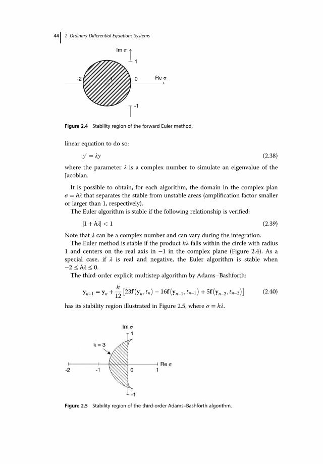
linear equation to do so:

y´ � λy (2.38)

where the parameter λ is a complex number to simulate an eigenvalue of theJacobian.

It is possible to obtain, for each algorithm, the domain in the complex planσ � hλ that separates the stable from unstable areas (amplification factor smalleror larger than 1, respectively).The Euler algorithm is stable if the following relationship is verified:

1 � hλj j < 1 (2.39)

Note that λ can be a complex number and can vary during the integration.The Euler method is stable if the product hλ falls within the circle with radius

1 and centers on the real axis in �1 in the complex plane (Figure 2.4). As aspecial case, if λ is real and negative, the Euler algorithm is stable when�2 � hλ � 0.The third-order explicit multistep algorithm by Adams–Bashforth:

yn�1 � yn � h12

23f yn; tn� � � 16f yn�1; tn�1

� � � 5f yn�2; tn�2� ��

(2.40)

has its stability region illustrated in Figure 2.5, where σ � hλ.

Im σ

Re σ-1-2 0

-1

1

Figure 2.4 Stability region of the forward Euler method.

Figure 2.5 Stability region of the third-order Adams–Bashforth algorithm.


The third-order implicit Adams–Moulton algorithm:

yn�1 � yn � h12

5f yn�1; tn�1� � � 8f yn; tn

� � � f yn�1; tn�1� ��

(2.41)

has its stability region illustrated in Figure 2.8.The region that is of most interest from a stability point of view is where the

Re λ� � < 0, since we wish to check the algorithm’s stability when the equation iswell conditioned. Generally speaking, we can lay down the following rules.

1) An implicit method is more stable than an explicit method with the sameorder.

2) Algorithm stability decreases as algorithm order increases.

An algorithm is A-stable if the amplification factor is smaller than 1 for eachpositive value of h when the algorithm is applied to a well-conditioned problem(with Re λ� � < 0).An A-stable algorithm has all the left semiplane as its stability domain.

The Euler backward method, for example, is A-stable since

κ � 11 � hλ

< 1; for hλ ! � ∞ (2.42)

The trapezium algorithm also is A-stable since

κ � 1 � 0:5hλ1 � 0:5hλ

�� < 1; for hλ ! � ∞ (2.43)

It seems that the trapezium algorithm is superior to the Euler backwardmethod from all viewpoints: Even though they are both A-stable and need tosolve a nonlinear system in yn�1, the trapezium algorithm is of second order,while Euler backward is of first order only. However, there is also an additionalaspect to consider.

An algorithm is strongly A-stable if κ ! 0 when hλ ! � ∞ .

For example, the Euler backward is strongly A-stable, whereas the trapeziumalgorithm is not. Actually, the trapezium algorithm has κ ! 1, while hλ ! � ∞ .To understand the importance of this feature, let us consider the reference

equation (2.38) with the initial condition y 0� � � y0. If t ! ∞ , the solution tendsto zero with Re λ� � < 0. If the initial condition is perturbed so as to have y0 � ε,the error with the trapezium algorithm propagates in line with the followingrelation:

en � 1 � �hλ=2�1 � �hλ=2� n

ε; n � 1 (2.44)


If Re λ� �j j is large, the amplification factor (the value of the ratio in (2.44)) tendstoward �1 and the error en does not tend toward 0: Any perturbation propagateswithout being dampened.Conversely, in the case of the Euler backward, we have

en � 11 � hλ

n

ε; n � 1 (2.45)

In this instance, en tends very fast toward 0 also for the large Re λ� �j j.One-step algorithms are always stable for h ! 0. In the case of multistep algo-rithms, the stability problem is further complicated by the presence of parasitesolutions, which can prevail on the real solution and make the algorithmunstable even for h ! 0.

To tackle this problem, let us consider the central point multistep algorithm:

yn�1 � yn�1 � 2hf yn; tn� �

(2.46)

which when applied to the reference equation (2.38) becomes

yn�1 � yn�1 � 2hλyn; n � 1 (2.47)

The solution of this equation with finite-differences is given by the relationship:

yn � b1rn1 � b2r

n2 ; n � 0 (2.48)

where r1 and r2 satisfy

rn�1 � rn�1 � 2hλrn (2.49)

that is

r2 � 1 � 2hλr (2.50)

and that results in

r1 � hλ �ffiffiffiffiffiffiffiffiffiffiffiffiffiffiffiffiffi1 � h2λ2

p; r2 � hλ �

ffiffiffiffiffiffiffiffiffiffiffiffiffiffiffiffiffi1 � h2λ2

p(2.51)

b1 and b2 are obtained by imposing the two conditions:

b1 � b2 � y0 (2.52)

b1r1 � b2r2 � y1 (2.53)

If h ! 0, the relation (2.48) becomes

yn � b1 exp λtn� � � b2 �1� �n exp �λtn� �; n � 0 (2.54)

The first term properly tends to the solution of the original differential equa-tion, whereas the second term tends to exponentially increase (if λ < 0, that is, awell-conditioned equation) and to alternate the sign. The reason is that thefinite-difference equation (2.47) is of the second order, whereas the originalequation was of the first order; therefore, two conditions y0 and y1 are needed to


solve the finite-difference equation, whereas only the condition y0 sufficed forthe original equation.The finite-difference equation is thus the summation of two terms, with only

the former coming from the original differential equation, whereas the latter oneis spurious and unstable.

This form of instability does not decrease with h ! 0. On the contrary, the errorat an assigned value tF increases while the integration step decreases since thenumber of times that we carry out an unstable calculation increases.

For example (Rice, 1993), the differential equation

y´ � 0:5y � �4=x� � 12x2

� f x; y� �; y 1� � � ffiffiffie

p � 1

is well conditioned and its analytical solution is

y � e1��x=2� � 1x2

If we assume we know the exact values of y in x � 1 � h, x � 1 � 2h, x � 1 � 3h,beyond x � 1, it is possible to use the following integration formula (central dif-ferences with five points):

y x � 4h� � � y x� � � 8y x � h� � � 12f x � 2h; y x � 2h� �� 8y x � 3h� �This formula is highly accurate (small local error), but it is unstable in

solving this problem whatever the integration step h is. Contrary to what wemight think, if we decrease the integration step, things actually worsen. Infact, in this case, the algorithm’s instability is linked solely to the number ofsteps, and after 5 steps we lose 5 significant digits, after 20 steps we lose 18digits, and so on.

To have a stable multistep algorithm, the parasite solutions must be negligiblewith respect to the real solution of the problem. The more the information fromthe previous points is used, the more the side solutions are inserted.

For example, the fourth-order Adams–Bashforth method applied to (2.38)generates the following fourth-order finite-difference equation:

yn�1 � yn � hλ24

55yn � 59yn�1 � 37yn�2 � 9yn�3� �

(2.55)

which has the general solution:

yn � C1rn1 � C2r

n2 � C3r

n3 � C4r

n4 (2.56)

Thus, it has three side solutions overlapped with the real solution. For h ! 0, thefirst root tends to the solution of the original differential equation, whereas the


others tend to

rij j < 1; i � 2; 4 (2.57)

Therefore, the side solutions do not generate any instability.Multistep algorithms have an additional limitation to their stability.

In a famous theorem, Dahlquist (1963) demonstrated that it is not possible tofind A-stable multistep algorithms and, obviously, strongly A-stable algorithms,of order larger than 2.

We will provide a way around this limitation later in this chapter.

In the previous procedure, we did not account for the effect of round-off errorson the global solution. In the most of cases, this error is negligible with respectto the local error, but it can become significant when the number of integrationsteps is quite large.

Specifically, there are two situations in which we cannot neglect the round-offerror:

1) When the method has a large local error (i.e., the Euler method), there isthe need to use a very small integration step and, hence the number ofsteps can become very large.

2) When the value of y is required in correspondence with ti, which aredenser than necessary to guarantee the method is accurate. This situationtypically occurs in image processing problems.

As we will see later, certain algorithms (multivalue methods) can bypass thislimitation since they allow the separation of the integration step effectively usedfrom the points ti requested by the user.

2.5Stiff Systems

We saw that to integrate the following differential equation:

y´ � �1000y � 1000; y 0� � � 10

using the Euler method, it is necessary to also adopt an extremely small integra-tion step when the solution is definitely constant.

In many practical applications, the integration of well-conditioned systems car-ried out using traditional methods requires a very small integration step toensure algorithm stability. Such a step is generally much smaller than requiredto ensure reasonable method accuracy.


This fact perplexed the pioneers who tackled the first ODE problems numeri-cally because they were unaware of two phenomena: the well conditioning andill-conditioning of systems and numerical algorithm stability.

The phenomenon for which the step size is progressively decreased to an unac-ceptably small level by adopting a traditional algorithm in a region where thesolution curve is very smooth is known as stiffness. The systems that lead to thisapparently anomaly are called stiff systems.

Years ago, it was believed that the stiffness of a system was related to physicalproblems only, which involve differential equations with different timescales,such as when we have to model kinetics schemes of chemical reactions withboth very short (radical species) and long lives (molecular).To understand what causes stiffness under such circumstances, let us consider

the following example (Stoer and Bulirsch, 1983):

y1 � λ1 � λ22

y1 � λ1 � λ22

y2

y2 � λ1 � λ22

y1 � λ1 � λ22

y2

which has the general solution:

y1 t� � � C1 exp λ1t� � � C2 exp λ2t� �y2 t� � � C1 exp λ1t� � � C2 exp λ2t� �

If the system is solved by means of the Euler method:

y1� �

n � C1 1 � hλ1� �n � C2 1 � hλ2� �ny2� �

n � C1 1 � hλ1� �n � C2 1 � hλ2� �nTo achieve stability, the integration step must be such that

1 � hλ1j j < 1 and 1 � hλ2j j < 1

Suppose we have λ1 � �1 and λ2 � �10 000; thus, the system is well condi-tioned, since λ1 < 0 and λ2 < 0. Moreover, as we can see from the exact solutionof the problem, the term C2 exp λ2t� � plays a role for very small t only. Never-theless, the integration step is conditioned by the eigenvalue λ2 for large t toosince the relation 1 � hλ2j j < 1 must be satisfied. Using the Euler method for thiskind of situation, we are paradoxically forced to use a very small integration stepfor a negligible term. The same problem arises with many other algorithms, suchas the classical Runge–Kutta of the fourth order or explicit multistep methods(discussed later).

A well-conditioned differential system (where all the eigenvalues of the Jacobianhave a negative real part) is stiff when the ratio of the maximum to minimumeigenvalue is large.

2.5 Stiff Systems 49

A large ratio between the maximum and the minimum eigenvalue of theJacobian indicates a stiff situation; nevertheless, when a single well-condi-tioned differential equation is integrated on a large interval, it may also pres-ent the stiffness phenomenon if the adopted algorithm has a small stabilityregion.

It is therefore possible to modify the definition of stiff systems: A system is stiff ifthe real part of the eigenvalue of at least one equation is both negative and large;in other words, if it is very well conditioned.

Analogous to system conditioning, we could encounter two different problemswith the same solution, yet the first problem is nonstiff and the second problemis stiff.

Clearly, this phenomenon cannot be a property of the solution since it is thesame for both problems and must be a property of the differential system itself. Itis thus appropriate to speak of stiff systems.

It is important not to confuse the concept of stiff systems with the problem ofhard solutions. When a system is stiff, a special algorithm must be used.

2.6Multistep and Multivalue Algorithms for Stiff Systems

To integrate a stiff system, an algorithm with a sufficiently wide stability regionmust be used. The ideal situation is to use a strongly A-stable algorithm.

The multistep algorithms (and the derived multivalue algorithms) alsoencounter a difficulty already introduced with the Dahlquist theorem: There areno A-stable multistep algorithms with order larger than 2. For these algorithms,Gear (1971) proposed the following analysis. A multistep or multivalue algo-rithm is able to solve stiff problems if it has the following properties in the threeregions of Figure 2.6:

� Region I: h Re λ� � < �α. The algorithm must be stable. If α � 0, the algo-rithm is A-stable. As mentioned above, Dahlquist demonstrated that themultistep algorithms of orders higher than 2 cannot be A-stable.

By relaxing the A-stability requirements for negative and reasonably small, butnot null, values of α, Gear allowed multistep algorithms with orders of higherthan 2 to be found.

� Region II: �α < h Re λ� � < 0. The algorithm must also allow the transient ofthe fastest components (with Re λ� � � 0) to be properly described. Thus, thealgorithm must be stable and accurate in this region.� Region III: 0 < h Re λ� � < β. In this region, the system is slightly ill-condi-tioned. The algorithm must be accurate.


Moreover, if multistep, the algorithm must be such that the parasite solutionsare negligible with respect to the real solution in all the three regions.The external area with respect to these three regions is of interest in excep-

tional situations in the case of stiff systems; in other words, there is no need tocheck the stability and accuracy of the algorithm.To summarize, a multistep algorithm is predisposed to solve stiff problems if it

has the following simple features.

1) The algorithm is stable when stability is crucial.2) The algorithm is accurate when precision is required.

2.7Control of the Integration Step

In modern programs, the integration step is modified to adapt it to the localrequirements of the problem. Usually, hn selection is carried out to check thelocal error E of the algorithm. Later, we will consider the problem of the estima-tion of the local error for different algorithms and study a strategy to vary hnaccording to E.

At this point, a qualitative analysis of the following problem is crucial: Theglobal error consists of the sum of the local error and the propagation error.How can we control the global error by accounting only for the local error?

We should first consider the reference equation (2.38) with λ < 0 and inte-grated with the Euler algorithm.The local error of the Euler method is

E � y´´h22

(2.58)

h Re(λ)

h Im(λ)

−α

βII IIII

Figure 2.6 Gear’s regions.

2.7 Control of the Integration Step 51

and therefore it decreases with larger t, since the second derivative is

y´´ � λ2 exp λt� � (2.59)

and λ < 0. Thus, if the local error is calculated exactly, the integration step,which is based on the local error check only, can be increased for large t. Actu-ally, to ensure algorithm stability, and hence also control the portion of theglobal error caused by the propagation error, we must have

hλ � 1j j < 1

and therefore the integration step must be under a certain limit. If λ � 0, theamplification factor of the problem is high and the integration step must be keptvery small.

If the local error is estimated in an exact way (by inserting the analytical expres-sion of the second derivative in the local error), we may encounter problems inusing the local error only to control the global error, since large h values mightbe accepted for large t.

As it usually happens in a calculation program, if the error E is estimated numer-ically, there is a good probability that E is overestimated because of algorithminstability.

To keep the discussion simple, suppose we estimate the error using the for-mula (2.58) where the second derivative is calculated using the difference of twovalues of y´:

y´´ � yn � yn�1h

(2.60)

In this case, if we used the explicit Euler method, there is a good probabilitythat one or both the values of y´ belong to curves different from the exact solu-tion and, if λ � 0, they are very different from the exact ones. Thus, the esti-mate of y´´ is much larger than the exact value and, consequently, E isoverestimated and h must be kept very small.If we use the implicit backward Euler, the two values of y´ are very small and

the integration step could be kept large.Although qualitative, this discussion shows that controlling only the local

error is usually a good way to keep the integration step within the region ofalgorithm stability since E is overestimated as it exits such a region.


It is worth noting that there is no guarantee of the validity of the check: Some-times the control can be inadequate and the algorithm may become unstable.

2.8Runge–Kutta Methods

A Runge–Kutta method consisting of r terms can be represented in syntheticform using the vectors w and c and the matrix A:

yn�1 � yn � w1k1 � w2k2 � ∙ ∙ ∙ � wrkr (2.61)

ki � hf yn �Xrj�1

aijkj; tn � cih

!; i � 1; . . . ; r (2.62)

A can be seen as the sum of three matrices AL;AD;AR. AL consists of thecoefficients of the left side of A and null elsewhere, AD of the diagonal elementsof A and null elsewhere, and AR of the right side elements of A and nullelsewhere.

A Runge–Kutta method with nonzero coefficients only in AL is explicit; if thenonzero coefficients are in both AL and AD, it is diagonally implicit; if AR alsohas nonzero coefficients, the method is implicit.

Often, a Runge–Kutta method is represented using the following shorthandnotation:

c1 a11 a12 . . . a1rc2 a21 a22 . . . a2r. . . . . . ::: . . . . . .

cr ar1 ar2 . . . arr

w1 w2 . . . wr

(2.63)

For example, the explicit second-order Runge–Kutta (2.9)–(2.11) is representedas follows:

0 0 0

1 1 012

12

(2.64)

2.8 Runge–Kutta Methods 53

2.9Explicit Runge–Kutta Methods

To understand the mathematical bases of the Runge–Kutta methods, it is usefulto look at the simple case of an explicit second-order method applied to a singlefirst-order equation:

y´ � f y; t� � (2.65)

In this case, the following recursive formula is used:

yn�1 � yn � w1k1 � w2k2 (2.66)

where


(2.67)

k2 � hf yn � ak1; tn � bh� �

(2.68)

The parameters a; b;w1;w2 are selected to satisfy at best a Taylor expansionseries of the solution y t� �:

y tn�1� � � y tn� � � hy´ tn� � � h2

2y´´ tn� � � O h3

� �� y tn� � � hf y tn� �; tn� � � h2

2f f y � f t� �

n� O h3

� � (2.69)

If we expand the function f yn � ak1; tn � bh� �

in Taylor series, we obtain

f yn � ak1; tn � bh� � � f yn; tn

� � � ak1f y � bhf t � O h2� �

(2.70)

From (2.66), it results in

yn�1 � yn � w1 � w2� �hf n � w2h2 af f y � bf t� �

n� O h3

� �(2.71)

Comparing (2.71) and (2.69), we obtain

w1 � w2 � 1 (2.72)

w2a � 0:5 (2.73)

w2b � 0:5 (2.74)

Since there are three equations with four unknowns, there are infinite possibil-ities for selecting the four parameters. Explicit second-order Runge–Kutta meth-ods differ from each other according to their use of this degree of freedom.For example, a possible choice is

w1 � w2 � 0:5; a � b � 1


that leads to


k2 � hf yn � k1; tn � h� �

yn�1 � yn � k1 � k22

The same procedure is used for methods of different orders. Also in this casethere are degrees of freedom exploited to obtain methods with good accuracyand stability. The formulae can be immediately extended to the case of differen-tial equation systems (2.1): In a situation like this, writing the ki as vectors willsuffice.For example, if we evaluate

k1 � hnf yn; tn� �

k2 � hnf yn � k12; tn � hn

2

(2.75)

we can obtain either the modified forward Euler method:

yn�1 � yn � k2 (2.76)

or the improved forward Euler method:

yn�1 � yn � k1 � k22

(2.77)

The Runge–Kutta method, which was so popular for so long that it is knownas the classical Runge–Kutta, was the fourth-order method:


(2.78)

k2 � hf yn � 0:5k1; tn � 0:5h� �

(2.79)

k3 � hf yn � 0:5k2; tn � 0:5h� �

(2.80)

k4 � hf yn � k3; tn � h� �

(2.81)

yn�1 � yn � k1 � 2k2 � 2k3 � k46

(2.82)

While p-order Runge–Kutta methods, with p � 4, require p computations of thefunctions f , higher order methods need p � 1 computations.

For example, a fifth-order Runge–Kutta method needs six calculations of thefunctions f .

For this reason and because the fourth order is usually a good compromisebetween accuracy and the issues arising from the high-degree polynomial

2.9 Explicit Runge–Kutta Methods 55

approximations (see Buzzi-Ferraris and Manenti, 2010b), the fourth-orderRunge–Kutta algorithms are often preferred to the higher and lower ordermethods.

The fourth-order explicit Runge–Kutta algorithm has a slightly better stabilityregion than the Euler forward method.Explicit Runge–Kutta algorithms have the following advantages and

disadvantages.

1) They are efficient even when the solution is not approximated bypolynomials.

2) They are usually only slightly sensitive to discontinuities in the functions fof the system.

3) They require very little memory.4) It is easy to change the integration step at any time.5) The computational effort is relatively small. The overall computational

time can be favorable in the case of systems with short computingtimes.

1) The number of calculations is generally larger than other alternative meth-ods discussed later.

2) They are not good for stiff problems.3) The local error cannot be explicitly evaluated.4) They will not solve problems where the derivatives y´ are in implicit form

or in forms different from (2.1) in any instance.5) They will not solve a differential–algebraic system.6) They are not good at solving problems where the solution is needed for

very close steps (i.e., graphical problems), that is with h much smaller thanthe ones required by the algorithm’s precision.

When implementing a program with a Runge–Kutta method, two issues mustbe tackled:

� Calculation of the local error of the algorithm.� Strategy to select and modify automatically the integration step.

Since the alternative methods of evaluating the local error can exploit a com-mon strategy to automatically control the integration step, we discuss the latterpoint first.

2.9.1

Strategy to Automatically Control the Integration Step

For the sake of simplicity, let us start with a single differential equation. Let ussuppose that we are able to estimate the local error of the p-order algorithm we


selected for the integration:

E � C h� �p�1 (2.83)

If it results in

E � ε (2.84)

the integration is repeated with a new, smaller, integration step; conversely, if theerror is satisfactory, the integration step can be increased. The strategy toincrease or decrease the step might be as follows.The integration step hnew must be such that

C hnew� �p�1 � ε (2.85)

Hence,

C h� �p�1 hnew� �p�1 � E hnew� �p�1 � ε h� �p�1 (2.86)

and therefore

hnew � hε

E

� �1=�p�1�(2.87)

This formula for the calculation of the new integration step needs certainimprovements since it is suitable to the following:

1) Insert a safety coefficient α < 1 to prevent the possible multiple repetitionof the step reduction at the same point. If such a coefficient is too small,the problem of increasing the number of good steps arises. Thus, the mostfrequent values are 0:7 � α � 0:8.

2) Control both the absolute and relative errors (Buzzi-Ferraris and Manenti,2010a). A good choice in most situations is

ε � εA � εR yn�� (2.88)

where εA stands for the absolute error and εR for the relative error. Thevalue of εR is related to the calculation precision.The formula (2.87) is modified as follows:

hnew � αhεA � εR yn

�� E

1=�p�1�(2.89)

3) Avoid small integration steps. This can happen when we select very smallvalues for εA; εR. Therefore, it is useful to perform a control on the selec-tion of these values and to assign a lower threshold to the integration step,under which the program exits with an error.

4) Assign an upper limit to the integration step increase to prevent the risk ofsuddenly reducing the same step.

5) In the case of differential systems with N > 1 equations, various differentalternatives are possible. A simple one is to use the test (2.89) for each


component, calculate the appropriate hnew for all of them, and select theminimum value. Looking at the Hindmarsh (1983) analysis, it seems to bepreferable to use the following strategy. The integration must be repeatedif it results in

e �ffiffiffiffiffiffiffiffiffiffiffiffiffiffiffiffiffiffiffiffiffiffiffiffiffiffi1N

XNi�1

Ei

εi

2vuut > 1 (2.90)

but is accepted otherwise. In relation (2.90), each component can have adifferent value of εA and εR. The new step is

hnew � αh1e

1=�p�1�(2.91)

2.9.2

Estimation of the Local Error

Many alternatives have been proposed to calculate the local error of Runge–Kutta algorithms. The main ones are as follows:

1) The use of an additional calculation of the system to have a degree of free-dom more. The most common method exploiting this possibility is theMerson method.

2) Richardson extrapolation.3) Embedded formulae.

For the sake of simplicity, we consider the case of a single differential equa-tion. With a differential equations system, we need Equation 2.90.

2.9.2.1 Runge–Kutta–Merson AlgorithmMerson proposed the following fourth-order algorithm that uses five functionevaluations:


(2.92)

k2 � hf yn � k13; tn � h

3

(2.93)

k3 � hf yn � k16� k2

6; tn � h

3

(2.94)

k4 � hf yn � k18� 3k3

8; tn � h

2

(2.95)


k5 � hf yn � k12� 3k3

2� 2k4; tn � h

(2.96)

yn�1 � yn � k16� 2k4

3� k5

6(2.97)

The local error of the algorithm can be calculated as follows:

E � 2k1 � 9k3 � 8k4 � k530

(2.98)

2.9.2.2 Richardson ExtrapolationThis technique has been described in Buzzi-Ferraris and Manenti (2010b), towhich we refer readers for further details. Let us denote with y2h and yh the val-ues of y in tn � 2h obtained, respectively, using the p-order Runge–Kuttamethod with step 2h and the p-order Runge–Kutta method with two steps oflength h each.If we also denote the expected value with y tn � 2h� �, in the first case, we have

y2h � y tn � 2h� � � C 2h� �p�1 (2.99)

and in the second case:

yh � y tn � 2h� � � 2C h� �p�1 (2.100)

Therefore, the local error can be estimated using the relation:

E � C h� �p�1 � yh � y2h�� 2p�1 � 2

(2.101)

Once yh is accepted, it can be improved using the equation (see Buzzi-Ferrarisand Manenti, 2010b):

yn�1 � yn � yh � y2h2p � 1

(2.102)

By doing this, the order used to calculate yn�1 is p � 1. A word of warning, how-ever: While the accuracy of yh is controlled by (2.101), it is no longer true foryn�1; it is not always true that the solution improves by increasing the order ofthe algorithm!

2.9.2.3 Embedded Algorithms

In the Runge–Kutta algorithms, there are degrees of freedom in the choice of theparameters that characterize each algorithm. It is possible to exploit these degrees offreedom to use the same elements for different algorithms of rising orders.

When several algorithms can use the same ki, they are indicated as embeddedalgorithms.


Let us consider, for example, the following third-order algorithm:


(2.103)

k2 � hf yn � k12; tn � h

2

(2.104)

k3 � hf yn � k1 � 2k2; tn � h� �

(2.105)

yn�1 � yn � k16� 2k2

3� k3

6(2.106)

The same values of k1 and k2 can be used for two other algorithms, the first forthe first order (Euler):

yn�1 � yn � k1 (2.107)

and the second for the second order:

yn�1 � yn � k2 (2.108)

In this case, we have three algorithms that use the same values of ki and hencewe can use the highest-order algorithm to estimate the error of the lower orderalgorithms in a simple manner.The most widespread embedded Runge–Kutta algorithms have a p-order

method controlled by a p � 1� �-order method. Let us denote with yp and yp�1the values of y in tn � h obtained using the p- and p � 1� �-order Runge–Kuttamethod. If y tn � h� � is the expected value, in the first case we have

yp � y tn � h� � � C h� �p�1 (2.109)

and in the second case:

yp�1 � y tn � h� � � D h� �p�2 (2.110)

Thus, the local error can be estimated through the relation:

E � C h� �p�1 � yp � yp�1�� (2.111)

since D h� �p�2 is negligible as it is of a higher order.One of the most popular embedded Runge–Kutta methods is the fourth-order

Runge–Kutta–Fehlberg method controlled by a fifth-order one. The equationsthat define it are as follows:


(2.112)

k2 � hf yn � k14; tn � h

4

(2.113)

k3 � hf yn � 3k132

� 9k232

; tn � 3h8

(2.114)


k4 � hf yn � 1932k12197

� 7200k22197

� 7296k32197

; tn � 12h13

(2.115)

k5 � hf yn � 439k1216

� 8k2 � 3680k3513

� 845k44104

; tn � h

(2.116)

k6 � hf yn � 8k127

� 2k2 � 3544k32565

� 1859k44104

� 11k540

; tn � h2

(2.117)

y4 � yn � 25k1216

� 1408k32565

� 2197k44104

� k55

(2.118)

y5 � yn � 16k1135

� 6656k312825

� 2856k456430

� 9k550

� 2k655

(2.119)

Usually, the value for yn�1 is the fifth-order value. A word of warning, however:Whereas yn�1 is calculated with the fourth-order algorithm and the precision iscontrolled by a fifth-order algorithm, it is no longer true for the fifth-order yn�1;it is not always true that the solution improves by increasing the algorithm order!

Many other formulae have been proposed and the basic idea has also beenexploited in other ways, leading to slightly different algorithms.

The Runge–Kutta–Fehlberg variant is usually slightly better than the other variants.

2.10Classes Based on Runge–Kutta Algorithms in the BzzMath Library

The following classes for the solution of nonstiff problems, which are based onRunge–Kutta explicit algorithms, are implemented in the BzzMath library:

� BzzOdeRK. Classical fourth-order Runge–Kutta method with check of theerror obtained by means of a reintegration with a halved step.� BzzOdeRKF. Fourth/fifth-order Runge–Kutta–Fehlberg method.� BzzOdeRKM. Fourth-order Runge–Kutta–Merson method.� BzzOdeRKS. Similar to the Fehlberg variant, fourth/fifth-order Runge–Kutta–Sarafyan method.

BzzOdeRK, BzzOdeRKF, BzzOdeRKM, and BzzOdeRKS classes have just oneconstructor that requires the following variables as their argument:

� The BzzVector y0, which contains the initial values of y, y0. If a singleequation is to be integrated, the vector has dimension 1.� The double t0, value of t0 (initial value of the independent variable).� The name of the function where the system is calculated.

2.10 Classes Based on Runge–Kutta Algorithms in the BzzMath Library 61

For example:

//function prototypevoid OdeSample(BzzVector &y,double t,BzzVector &f);. . .

double t0 = 0.;BzzVector y0(3,2.,1.,2.);//object definitionBzzOdeRKF o(y0,t0,OdeSample);

The user must provide the prototype declaration for the function where thesystem is calculated, f y; t� �, before defining an object that uses it within the pro-gram. The function input is the vector y and the corresponding t, which aremanaged by the object. The output is the vector f . For efficiency purposes aswell as for easiness of use, the vectors y and f are both BzzVector references.The function argument reads as follows:

(BzzVector &y,double t,BzzVector &f)

Within the definition of the function, the elements of y and f are available bymeans of the operator [], if maximum efficiency is needed, or using (), if theaccess validity check is useful.

The user must not modify the values of y inside this function.

Example 2.1

Integrate the following nonstiff system (Lapidus and Seinfeld, 1971):

y1 � �0:1y3 � 49:9y2y2 � �50y2y3 � 70y2 � 120y3

with initial conditions y1 0� � � 2; y2 0� � � 1; y3 0� � � 2 within the interval0 � t � 0:1, using a program based on the algorithms of the Runge–Kutta familyimplemented in the BzzMath library.The program is


//prototypevoid OdeExample1(BzzVector &y,double t,

BzzVector &f);void main(void)

{BzzVector y0(3,2.,1.,2.),y;double tOut = 0.1;


BzzOdeRK oRK(y0,0.,OdeExample1);y = oRK(tOut);oRK.BzzPrint(“Runge-Kutta Results”);BzzOdeRKM oRKM(y0,0.,OdeExample1);y = oRKM(tOut);oRKM.BzzPrint(“Runge-Kutta-Merson Results”);BzzOdeRKF oRKF(y0,0.,OdeExample1);y = oRKF(tOut);oRKF.BzzPrint(“Runge-Kutta-Fehlberg Results”);BzzOdeRKS oRKS(y0,0.,OdeExample1);y = oRKS(tOut);oRK.BzzPrint(“Runge-Kutta-Sarafyan Results”);}

void OdeExample1(BzzVector &y,double t,BzzVector &f){f[1] = � 0.1 * y[1] � 49.9 * y[2];f[2] = �50. * y[2];f[3] = 70. * y[2] � 120. * y[3];}

The total number of system evaluations is

BzzOdeRK: 340BzzOdeRKM: 214BzzOdeRKF: 257BzzOdeRKS: 359

An object from the previous classes, as it is defined, automatically receivesa default value for the tolerances of the absolute (1.e�10) and relative(1.e�6) errors on the variables yi.It is possible to modify the default values of such tolerances using the func-

tions SetTolAbs and SetTolRel, which accept as their argument both a singlevalue for all the variables or a BzzVector to assign a special tolerance to eachvariable:

BzzVector tolAbs(3,1.e�3,1.e�4,1.e�5);BzzVector tolRel(3,.001,.0001,.00001);double tolA = 1.e�5; // default 1.e�10double tolR = 1.e�4; // default 1.e�6o1.SetTolAbs(tolAbs);o2.SetTolRel(tolRel);o3.SetTolAbs(tolA);o4.SetTolRel(tolR);

An object from these classes remembers its history.

2.10 Classes Based on Runge–Kutta Algorithms in the BzzMath Library 63

If the use of the object for tOut progressively increased, the integration is notperformed by starting from t0 each time, but from the value of t achieved in theprevious iteration with an integration step already estimated. For example:

for(int i = 1;i <= 10;i++){y = o(tOut);tOut *= 10.;}

Objects from these classes allow the integration to be performed with anassigned number of steps. In this case, there is no control on the error generatedat each integration step. For example, the following statement is used to perform500 steps of integration:

y = o(tOut,500);

Additional examples of the use of BzzOdeRK, BzzOdeRKM, BzzOdeRKF, andBzzOdeRS classes can be found in

BzzMath/Examples/BzzMathAdvanced/Ode

directory and

OdeRungeKutta

subdirectory in the BzzMath7.zip file available at the web site:http://www.chem.polimi.it/homes/gbuzzi.

2.11Semi-Implicit Runge–Kutta Methods

Explicit Runge–Kutta methods are not suited to solving stiff systems, whereasthe implicit ones described later need to solve a generally nonlinear system ofequations. Semi-implicit Runge–Kutta methods derived from diagonally implicitmethods only seemingly allow overcoming the difficulties of implicit methodsand to be at the same time good candidates to handle stiff problems. They comefrom a Rosembrock idea (Chan et al., 1978). Semi-implicit methods are appliedto the systems in their autonomous form:

y´ � f y� �; y0 � y t0� � (2.120)

to exploit the Rosembrock device.To illustrate the principle this device is based on, let us consider the following

two-terms semi-implicit Runge–Kutta method:

yn�1 � yn � w1k1 � w2k2 (2.121)

k1 � hf yn � a11k1� � � hf yn

� � � ha11J yn� �

k1 (2.122)



k2 � hf yn � a21k1 � a22k2� � � hf yn � a21k1

� � � ha22J yn � a21k1� �

k2

(2.123)

As we can see in (2.122) and (2.123), the functions f are expanded in Taylor series;in this way, once the characteristic parameters w1;w2; a11; a21; a22 and the values off and J are known, it is possible to calculate k1; k2 by solving the linear systems:

I � ha11J yn� ��

k1 � hf yn� �

(2.124)

I � ha22J yn � a21k1� ��

k2 � hf yn � a21k1� �

(2.125)

The characteristic parameters of the different methods are selected to give themethod certain particular features, such as stability, accuracy, and computationaleffort, to obtain ki.One of the most successful methods is the Michelsen method, obtained as a

small variant on the Caillaud–Padmanabhan method (Chan et al., 1978):

I � haJ yn� ��

k1 � hf yn� �

(2.126)


k2 � hf yn � bk1� �

(2.127)


k3 � ck1 � dk2 (2.128)

The Michelsen method is a third-order method and is strongly A-stable. Itrequires, at each iteration, only one calculation of J, two calculations of f , and asingle factorization for the solution of the three systems (since they have thesame matrix of coefficients, see Buzzi-Ferraris and Manenti, 2010b).The Michelsen method has an additional advantage: Chan et al. (1978) dem-

onstrated that the same values of ki can be used to form, in addition to the third-order Michelsen method, another first-order method, which is hence embedded,that also turns out to be strongly A-stable:

yn�1 � yn � v1k1 � v2k2 (2.129)

having v1 � 0:6721 and v2 � 0:3278.It is thus possible to check the step and the error with the same technique

used with the embedded explicit Runge–Kutta methods.

The semi-implicit Michelsen method has the advantage of being third order andstrongly A-stable without requiring, as per the implicit methods, the solution ofa nonlinear system. Moreover, the control of the error can be performed with anembedded first-order method, also strongly A-stable.

What initially seems to be an advantage of the semi-implicit methods is reallya negative. In the semi-implicit methods, the Jacobian is directly within the defi-nition of the same method; in the implicit methods, it is used (if we use a Newtonmethod for the nonlinear system solution) only indirectly, solely for the solutionof the nonlinear system. Thus, the semi-implicit methods have the followingdisadvantages.

2.11 Semi-Implicit Runge–Kutta Methods 65

1) The Jacobian of the system must be calculated with extreme accuracy(since it is an intrinsic part of the method).

2) The Jacobian must be known with a degree of high accuracy at each inte-gration step (it cannot be kept constant for many steps when it slightlyvaries).

3) The matrices used to solve the linear systems must be refactorized at eachintegration step (due to the Jacobian changes).

Consequently, the semi-implicit methods can be considered to solve stiff systemsonly when the Jacobian can be calculated analytically and is not too computa-tionally expensive with respect to the evaluation of the system f .

2.12Implicit and Diagonally Implicit Runge–Kutta Methods

Many different methods for these Runge–Kutta categories have been proposed.The one that follows, for example, is an implicit third-order Runge–Kuttamethod that is strongly A-stable (Cash method) (Chan et al., 1978):

yn�1 � yn � k1 � 2k2 � 2k3 � k46

(2.130)

with

k1 � hf yn�1; tn�1� �

(2.131)

k2 � hf yn�1 � k12; tn�1 � h

2

(2.132)

k3 � hf yn�1 � k22; tn�1 � h

2

(2.133)


(2.134)

To calculate ki, it is necessary to solve the nonlinear systems (2.130)–(2.134)with respect to the unknowns, k1, k2, k3, and yn�1. The method is embeddedwith a second-order method, which is also A-stable:

yn�1 � yn � k2 (2.135)

A disadvantage of the implicit Runge–Kutta methods that contain other implicitembedded methods is that we must solve the nonlinear system related to theoverall method and the system related to the embedded method as well.


For instance, in the case of Cash’s method, we must solve the system

yn�1 � yn � k1 � 2k2 � 2k3 � k46

(2.136)

and the system

yn�1 � yn � k2 (2.137)

since the vector k2 that is in (2.132) is different from the one in (2.137).Other examples of implicit Runge–Kutta algorithms include the backward

Euler methods:

k1 � hnf yn�1; tn�1� �

(2.138)

yn�1 � yn � k1 (2.139)

and the improved backward Euler (also called the second-order Gear) method:

k1 � hnf yn; tn� �

(2.140)

k2 � hnf yn�1; tn�1� �

(2.141)

yn�1 � yn � 2k1 � k23

(2.142)

Some recent Runge–Kutta formulae are based on quadrature methods, that is,the points at which the intermediate stage approximations are taken are thesame points used in integration with either Gauss or Lobatto or Radau rules(Chapter 1). For example, the Runge–Kutta method derived from the Lobattoquadrature with three points (also called the Cavalieri–Simpson rule) is

k1n � hnf yn; tn� �

(2.143)

k2n � hnf yn � 524

k1n � 13k2n � 1

24k3n; tn � hn

2

(2.144)

k3n � hnf yn � 16k1n � 2

3k2n � 1

6k3n; tn � hn

(2.145)

yn�1 � yn � 16k1n � 2

3k2n � 1

6k3n (2.146)

and it is of fourth order.In the explicit Runge–Kutta methods, calculating the values of ki is not a

problem as they are explicit. In the implicit methods, however, it is necessary tosolve a nonlinear system and computational complexity increases.If the algorithm is diagonally implicit, the nonlinear system is much simpler to

solve.

Diagonally implicit methods are indicated with the acronym DIRK.

2.12 Implicit and Diagonally Implicit Runge–Kutta Methods 67

The semi-implicit version of diagonally implicit methods is obsolete since itrequires a very accurate calculation of the Jacobian J at each integration step. If,on the contrary, the Jacobian is used to apply the Newton method, such an accu-rate solution is no longer needed. The only necessary condition is to allow theconvergence of the Newton method.

This suggests that many diagonally implicit methods are still valid. The onlydifference is that the Jacobians are no longer included in the formula to evaluatey in the new point.

In the BzzMath library, classes based on implicit and diagonally implicit Runge–Kutta methods are not implemented to handle ODE problems with initialconditions.

2.13Multistep Algorithms

Multistep methods are characterized by the use of information collected in theprevious intervals integrated with constant h.

The general form of a multistep algorithm that uses the information of k previ-ous points is

yn�1 � a0yn � a1yn�1 � a2yn�2 � ∙ ∙ ∙ � akyn�k� h b�1f yn�1; tn�1

� � � b0f yn; tn� ��

� b1f yn�1; tn�1� � � ∙ ∙ ∙ � bk f yn�k ; tn�k

� �� (2.147)

In (2.147), there are 2k � 3 parameters: a0; a1; . . . ; ak ; b�1; b0; b1; . . . ; bk ; if wewish to have a p-order algorithm, p � 1 relations are needed. Thus, 2k � p � 2degrees of freedom are still available to obtain different algorithms with theirown features.

If b�1 � 0, the method is explicit; otherwise, the method is implicit.

For example, the following third-order Adams–Bashforth algorithm is explicit:

yn�1 � yn � h12

23f yn; tn� � � 16f yn�1; tn�1

� � � 5f yn�2; tn�2� ��

whereas the third-order Adams–Moulton is implicit:

yn�1 � yn � h12

5f yn�1; tn�1� � � 8f yn; tn

� � � 5f yn�1; tn�1� ��


The multistep methods have the following advantages with respect to the one-step methods of the same order.

1) They provide a trivial estimate of the local error.2) They require fewer computations for each integration step.

As already discussed, the Runge–Kutta methods require more computationsto estimate the local error. Conversely, the multistep methods allow the localerror to be estimated in a very simple way: For each p-order algorithm, there is acoefficient Cp such that the local error is

ep � Cpy p�1� � ξ� �hp�1; tn < ξ < tn�1 (2.148)

For example, the fourth-order Adams–Moulton algorithm:

yn�1 � yn � h24

9f yn�1; tn�1� � � 19f yn; tn

� � � 5f yn�1; tn�1� � � f yn�2; tn�2

� ��

has a truncation error:

e4 � � 19720

y 5� � ξ� �h5; tn < ξ < tn�1

and hence

C4 � � 19720

We will see later how it is possible to estimate the derivative y p�1� � ξ� � required toestimate the local error.A p-order Runge–Kutta method requires at least p calculations of the system

f y; t� � at each integration step; the same-order explicit multistep method needs asingle system evaluation.A great number of explicit and implicit multistep algorithms have been

proposed.

In the past, multistep algorithms were selected based on their local error in par-ticular because the importance of stability was not yet clear.

Many of these multistep methods (and also their modern multivalue versiondescribed later) that were of great interest in the past are now considered obso-lete due to their small stability region.

For instance, Milne’s method:

yn�1 � yn � 4h3

2f yn; tn� � � f yn�1; tn�1

� � � 2f yn�2; tn�2� �� 14

45h5y�5� ξ� �

(2.149)

2.13 Multistep Algorithms 69

has a rather favorable local error, but it is not used anymore due to its poorstability.

2.13.1

Adams–Bashforth Algorithms

If we assign

k � p � 1; a1 � a2 � ∙ ∙ ∙ � ap�1 � 0; b�1 � 0 (2.150)

the p-order Adams–Bashforth algorithm is obtained:

yn�1 � a0yn

� h b0f yn; tn� � � b1f yn�1; tn�1

� � � ∙ ∙ ∙ � bp�1f yn�p�1; tn�p�1� �h i

(2.151)

Since b�1 � 0, it is explicit. As the number of coefficients is equal to p � 1,there is no degree of freedom if we wish the relation (2.151) to be exact for ap-degree polynomial.The first six members of the family are as follows:

yn�1 � yn � hf yn; tn� � � 1

2y 2� �h2 (2.152)

yn�1 � yn � h2

3f yn; tn� � � f yn�1; tn�1

� �� 512

y 3� �h3 (2.153)

yn�1 � yn � h12

23f yn; tn� � � 16f yn�1; tn�1

� � � 5f yn�2; tn�2� ��

� 38y 4� �h4

(2.154)

yn�1 � yn � h24

55f yn; tn� � � 59f yn�1; tn�1

� ��37f yn�2; tn�2

� � � 9f yn�3; tn�3� �� 251

720y 5� �h5

(2.155)

yn�1 � yn � h720

1901f yn; tn� � � 2774f yn�1; tn�1

� ��2616f yn�2; tn�2

� � � 1274f yn�3; tn�3� � � 251f yn�4; tn�4

� �� 95288

y 6� �h6 (2.156)

yn�1 � yn � h1440

4277f yn; tn� � � 7923f yn�1; tn�1

� � � 9982f yn�2; tn�2� ��

�7298f yn�3; tn�3� � � 2877f yn�4; tn�4

� � � 475f yn�5; tn�5� ��

� 1908760480

y 7� �h7 (2.157)


2.13.2

Adams–Moulton Algorithms

If we assign

k � p � 2; a1 � a2 � ∙ ∙ ∙ � ap�2 � 0 (2.158)

the p-order Adams–Moulton algorithm is obtained:

yn�1 � a0yn

� h b�1f yn�1; tn�1� � � b0f yn; tn

� � � ∙ ∙ ∙ � bp�2f yn�p�2; tn�p�2� �h i

(2.159)

Since b�1 ≠ 0, it is implicit. As the number of coefficients is equal to p � 1,there is no degree of freedom if we wish the relation (2.159) to be exact for ap-degree polynomial.The first six members of the family are as follows:

yn�1 � yn � hf yn�1; tn�1� � � 1

2y 2� �h2 (2.160)

yn�1 � yn � h2

f yn�1; tn�1� � � f yn; tn

� �� 112

y 3� �h3 (2.161)

yn�1 � yn � h12

5f yn�1; tn�1� � � 8f yn; tn

� � � f yn�1; tn�1� �� 1

24y 4� �h4

(2.162)

yn�1 � yn � h24

9f yn�1; tn�1� � � 19f yn; tn

� ��5f yn�1; tn�1

� � � f yn�2; tn�2� �� 19

720y 5� �h5

(2.163)

yn�1 � yn � h720

251f yn�1; tn�1� � � 646f yn; tn

� ��264f yn�1; tn�1

� � � 106f yn�2; tn�2� � � 19f yn�3; tn�3

� �� 3160

y 6� �h6(2.164)

yn�1 � yn � h1440

475f yn�1; tn�1� � � 1427f yn; tn

� � � 798f yn�1; tn�1� ��

� 482f yn�2; tn�2� � � 173f yn�3; tn�3

� � � 27f yn�4; tn�4� ��

� 86360480

y 7� �h7(2.165)

Multistep methods have the following shortcomings.

1) All the explicit algorithms are unstable and, therefore, the implicit onesmust be used. Consequently, a nonlinear system has to be solved at eachiteration.

2.13 Multistep Algorithms 71

2) In this version, the algorithms are not self-containing: They need someother methods (i.e., a Runge–Kutta of the same order) to calculate thepoints involved in the formula in advance.

3) The formulae are predisposed for an integration with constant step.If we wish to change the integration step, several tough problems arise(e.g., a Runge–Kutta method has to be used as per the initializationproblem).

The multistep methods are only of historical interest since their correspondingmultivalue versions are used nowadays.

2.14Multivalue Algorithms

The implementation of the multistep methods is ineffective for general differen-tial equation numerical integration programs because of their complex initializa-tion and variation in the integration step.

All these problems are removed by implementing a small change of perspective.As underlined in the previous volume (Vol. 2, Buzzi-Ferraris and Manenti,2010b), a polynomial can be represented and collected in many ways. The tradi-tional approach used in the multistep methods is based on the collection of thesupport points yn; tn

� �, yn�1; tn�1� �

, yn�2; tn�2� �

, . . . ; the same polynomial canbe represented by collecting the ordinate of the different derivatives in corre-spondence with a single point tn: yn; tn

� �, yn; tn� �

, y´n; tn� �

, . . . .

To better understand this new way of looking at the problem, we can take theexample of a particular algorithm, such as the fourth-order Adams–Moultonalgorithm in its multivalue version.

For each multistep algorithm, there is a corresponding multivalue algorithmwith the same features.

Let us suppose that the method has been already initialized and that we are atthe generic integration point tn. The previous history of the algorithm is col-lected in a vector z.

Nordsieck proposed an efficient way of collecting the information called theNordsieck vector.


The Nordsieck vector consists of

z0 � yn

z1 � hyn

z2 � h2y´n2

z3 � h3y 3� �n

6

z4 � h4y 4� �n

24When we solve a differential system, each element of the Nordsieck vector is, inturn, a vector; in other words, z is usually a matrix. In such cases, it is preferableto consider the Nordsieck vector as a vector of vectors.

If the exact (no errors) elements of the Nordsieck vector z were known at tn,we could write the following Taylor expansion series for each element:

y tn�1� � � y tn� � � hy´ tn� � � h2y´´ tn� �2

� h3y 3� � tn� �6

� h4y 4� � tn� �24

� h5y 5� � tn� �120

� ∙ ∙ ∙

hy´ tn�1� � � hy´ tn� � � 2h2y´´ tn� �

2� 3

h3y 3� � tn� �6

� 4h4y 4� � tn� �

24� 5

h5y 5� � tn� �120� ∙ ∙ ∙

h2y´´ tn�1� �2

� h2y´´ tn� �2

� 3h3y 3� � tn� �

6� 6

h4y 4� � tn� �24

� 10h5y 5� � tn� �

120� ∙ ∙ ∙

h3y 3� � tn�1� �6

� h3y 3� � tn� �6

� 4h4y 4� � tn� �

24� 10

h5y 5� � tn� �120

� ∙ ∙ ∙

h4y 4� � tn�1� �24

� h4y 4� � tn� �24

� 5h5y 5� � tn� �

120� ∙ ∙ ∙

The vector z allows us to calculate a vector v, which is an approximation ofthe Taylor series above:

v0 � z0 � z1 � z2 � z3 � z4v1 � z1 � 2z2 � 3z3 � 4z4v2 � z2 � 3z3 � 6z4v3 � z3 � 4z4v4 � z4

and in matrix form:

v � Dz (2.166)

where D is the Pascal triangular matrix with coefficients:

dij � j!j � i� �!i! ; j � i � 0 (2.167)

2.14 Multivalue Algorithms 73

The vector v can be obtained without performing the product (2.166) betweenmatrix and vector, but simply through sums of vectors.

The required program is

for(i = 0;i <= orderUsed;i++)v[i] = z[i];

for(i = 0;i <= orderUsed;i++)for(j = orderUsed - 1;j >= i;j++)v[j] += v[j+1];

The vector v can be considered as a prediction of z in the new point tn�1, builtup using the same z known at tn.

The prevision v is corrected (through specific procedures, depending on thealgorithm) using an appropriate vector b, the value and scope of which will beshown below, so as to obtain the new vector z related to tn�1:

z0 � v0 � r0b (2.168)

z1 � v1 � r1b (2.169)

z2 � v2 � r2b (2.170)

z3 � v3 � r3b (2.171)

z4 � v4 � r4b (2.172)

Each p-order multivalue is characterized by the vector r used to correct the pre-diction v. It corresponds to the coefficients a0, a1, . . . , b�1, b0, . . . , bk used inthe multistep methods and is selected to make the algorithm stable, accurate,and exact for the p-degree polynomial solutions.

For example, the fourth-order Adams–Moulton method is characterized bythe following vector:

rT � 38; 1;

1112

;13;124

�

and therefore in this case the vector z in tn�1 is obtained through the followingrelations:

z0 � v0 � 38b

z1 � v1 � b

z2 � v2 � 1112

b

z3 � v3 � 13b

z4 � v4 � 124

b


The vector b is calculated to have z that satisfies the differential system in thenew point.

Since the system (2.1) is considered:

y´ � f y; t� �it becomes

hy´ � z1 � hf z0; t� � (2.173)

and results in

v1 � b � hf v0 � r0b; tn�1� � (2.174)

Thus, for the Adams–Moulton method, the result is

v1 � b � hf v0 � 38b; tn�1

As we can see, the Adams–Moulton method is implicit even in its multivalue

form.

One very important consequence of this new formulation is that we can nowalso handle problems that are not in the special form (2.1).

Suppose we have a system in the following implicit form:

f y m� �; y m�1� �; . . . ; y´; y; t� � � 0 (2.175)

In this case, it is sufficient to replace each derivative with the correspondingcomponent of the Nordsieck vector to have a nonlinear system in the singleunknown b. For example, in the case of implicit first-order multivalue methods,the following system must be solved:

fv1 � b

h; v0 � r0b; tn�1

� 0 (2.176)

Another important case is

Ay´ � f y; t� � (2.177)

where A is an assigned matrix. The nonlinear system is

A v1 � b� � � hf v0 � r0b; tn�1� � (2.178)

The previous formulation of a differential system is quite important for tworeasons.

1) Many practical problems come into being in this form and are broughtback to the standard form by manipulating the equations. It is thereforepreferable to face the solution directly in the primitive form.


2) If the matrix A is singular, the resulting system is differential–algebraic.This formulation also allows handling this important problem.

It seems that this new formulation allows solving problems in which the deriv-atives of any order are implicit or with differential–algebraic natures.

In practice, all the variants of the first-order explicit form (2.1) are more difficultto solve because of the resulting nonlinear system that we obtain. In fact, as willbe shown later, the formulation (2.1) provides the nonlinear system with a spe-cial feature.

Coming back to the explicit first-order system, the following issues are stillopen:

1) How to control the local error.2) How to change the integration step.3) How to vary the order of integration algorithm.4) How to contemporaneously select the step and the order.5) How to initialize a multivalue method.6) How to select the width of the first integration step.7) How to select the best multivalue algorithm.8) How to solve the nonlinear system (2.174).

2.14.1

Control of the Local Error

Each multivalue method is characterized by the same local error as the corre-sponding multistep method.For example, the multivalue fourth-order Adams–Moulton algorithm has the

same local error as the corresponding multistep fourth-order Adams–Moultonalgorithm:

yn�1 � yn

� h24

9f yn�1; tn�1� � � 19f yn; tn

� � � 5f yn�1; tn�1� � � f yn�2; tn�2

� �� which is

e4 � � 19720

y 5� � ξ� �h5; tn < ξ < tn�1

and hence

C4 � � 19720

The local error of a multivalue method is therefore obtained by means of

ep � Cpyp�1� � ξ� �hp�1 (2.179)


For certain reasons that we will explain soon, the error of a multivalue methodshould now be calculated in a slightly different way than the traditionalapproach, using the following expression:

ep � Epy p�1� � ξ� �hp�1

p � 1� �! (2.180)

withEp � Cp p � 1� �! (2.181)

For example, the fourth-order multivalue Adams–Moulton algorithm has alocal error:

e4 � � 19720

5!y 5� � ξ� �h55!

; tn < ξ < tn�1

Thus, it results in

E4 � � 19� �5!720

� �3:16666667

To estimate the local error of a p-order multivalue method, it is necessary tohave an approximate value for the p � 1� �-order derivative. It is trivial since wecollected the derivatives in the Nordsieck vector up to the order p.

The last element of z is

zp � hpy p� �n

p!(2.182)

If we know this element in correspondence with two adjacent points, tn�1 and tn,we can evaluate

y p�1� � ξ� �hp�1p � 1� �! � hpy p� �

n

p!� hpy p� �

n�1p!

!p!

p � 1� �! (2.183)

since

y p�1� � ξ� � � y p� �n � y p� �

n�1h

(2.184)

Thus, the local error can be estimated through the relation

Epy p�1� � ξ� �hp�1

p � 1� �! � Epzp� �

n � zp� �

n�1p � 1

(2.185)

In practice, it is appropriate to collect

zp�1 � zp� �

n � zp� �

n�1p � 1

� rpbp � 1

� y p�1� � ξ� �hp�1p � 1� �! (2.186)


in the element zp�1. The error is calculated as follows:

Epy p�1� � ξ� �hp�1

p � 1� �! � Epzp�1 � Cpp!rpb (2.187)

Once we have estimated the local error, it must be compared with the acceptablemaximum value. If it results in

ep � Ep

ffiffiffiffiffiffiffiffiffiffiffiffiffiffiffiffiffiffiffiffiffiffiffiffiffiffiffiffiffiffiffiffiffiffi1N

XNi�1

zi� �p�1εi

2vuut > 1 (2.188)

it is necessary to repeat the integration with a smaller step and, if convenient,with a different order of the method. Otherwise, the integration continues and,once again in this case, it can be useful to change the integration step and theorder of method as well. Later, we will suggest a strategy.

2.14.2Change the Integration Step

As we have seen for the Runge–Kutta methods, the integration steps must bereduced (and it is necessary to repeat the integration) when the local error islarger than a certain threshold assigned by the user. It can also be useful tochange the integration step when the local error is too small; in this case, it isbetter to enlarge it in the steps that follow to save calculations.

Although the integration step changes are rather difficult to perform in multi-step methods, they are quite easy with the multivalue methods. In fact, you onlyneed to scale the elements of z to adapt it to the new step!

If we want to change the integration step h to make it equal to hnew, the new zbecomes

z0 � z0

z1 � hnewh

z1

z2 � hnewh

2

z2

z3 � hnewh

3

z3

z4 � hnewh

4

z4

..

. ... ...

This feature of the multivalue methods is also exploited in another way and for acompletely different objective to the change of the integration step. In fact, it is


possible to make the integration step independent of the points for which we wantan answer!

It is worth remarking that the Nordsieck vector allows us to perform an inter-polation in the neighborhood of the current point tn; consequently, the predic-tion in a point hnew from tn is obtained using the relation

v0 � z0 � hnewh

z1 � hnew

h

2

z2 � hnewh

3

z3 � hnewh

4

z4 � ∙ ∙ ∙

(2.189)

The Nordsieck vector in tn allows us to perform the interpolation with therequired precision only between tn�1 and tn, which is for negative values of theratio hnew=h� � and with hnewj j � hj j � tn � tn�1j j.Using traditional integration programs, where it is possible to use a variable

integration step, the last step must be in line with requirements. This is no lon-ger needed in a program based on multivalue methods; in fact, if the last integra-tion step goes beyond the required point, it is sufficient to perform aninterpolation to obtain the right return within the acceptable range of error.This new possibility is very useful even when we need some values of y for

several points that are very close to each other (i.e., for graphical problems).Without this possibility (e.g., with the Runge–Kutta algorithms), an integrationwith a very small step is needed, but the step is much too small if we look at thealgorithm’s accuracy and stability.In the following, we will show how this feature can be exploited to solve some

special problems.

2.14.3Changing the Method Order

In the first differential equation integration programs, the order of the methodwas assigned by the user and was retained during the calculations. In manycases, however, it is more effective to modify it after the integration steps. Infact, there is an optimal integration step related to both the order of the methodadopted and the required accuracy.

It is essential to understand the following points:

1) How to estimate the elements of z with larger orders (e.g. zp�1; zp�2, . . . ).using a p-order algorithm.

2) How to change the order of the integration method.3) Why it might be useful to change the integration order.


We have seen that by using the zp element, it is possible to calculate the ele-ment zp�1:

zp�1 � zp� �

n � zp� �

n�1p � 1

� y p�1� � ξ� �hp�1p � 1� �! (2.190)

which is useful in obtaining an estimate of the local error of the p-orderalgorithm.Analogously, we can estimate the derivatives of higher orders or the elements

of the Nordsieck vector. Specifically, if we wish to evaluate zp�2, it is particularlyeasy if we collect three adjacent values of the last element zp in correspondencewith tn�2, tn�1, and tn. The result is

y p�2� � ξ� �hp�2p � 2� �! � hpy p� �

n

p!� hpy p� �

n�2p!

!p!

p � 2� �! (2.191)

Obviously, the same estimate could also come from the collection of two val-ues of the element zp�1:

y p�2� � ξ� �hp�2p � 2� �! � zp�1

� �n � zp�1� �

n�1p � 2

(2.192)

Thus, it is possible to estimate all the elements of z up to the maximum order(after an appropriate number of integration steps), starting from an algorithm ofany order.To understand how to change the order of the integration method, let us suppose

we are using the Adams–Moulton algorithms and that we have already initializedthem for the generic order p, which is smaller than the maximum order permitted.In this kind of instance, after an appropriate number of steps, the vector z will

have collected p � 2 elements z0; z1; . . . ; zp; zp�1. At this point, if we want to usea p � 1� �- or a p � 1� �-order integration method, we need to only use the propernumber of terms in the prediction v and the corresponding vector r to obtainthe correction b and the vector z in the new mesh point.For example, if the first- or third-order Adams–Moulton method is used and

we wish to use the second-order method, we have

v0 � z0 � z1 � z2v1 � z1 � 2z2v2 � z2

Next,

z0 � v0 � 12b

z1 � v1 � b

z2 � v2 � 12b

since the vector r of the second-order Adams–Moulton method is 1=2; 1; 1=2.


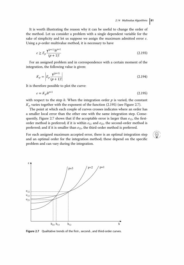
It is worth illustrating the reason why it can be useful to change the order ofthe method. Let us consider a problem with a single dependent variable for thesake of simplicity and let us suppose we assign the maximum admitted error ε.Using a p-order multivalue method, it is necessary to have

ε � Epy p�1� �hp�1p � 1� �! (2.193)

For an assigned problem and in correspondence with a certain moment of theintegration, the following value is given:

Kp � Epy p�1� �p � 1� �!

�� (2.194)

It is therefore possible to plot the curve:

ε � Kphp�1 (2.195)

with respect to the step h. When the integration order p is varied, the constantKp varies together with the exponent of the function (2.195) (see Figure 2.7).The point at which each couple of curves crosses indicates where an order has

a smaller local error than the other one with the same integration step. Conse-quently, Figure 2.7 shows that if the acceptable error is larger than e12, the first-order method is preferred; if it is within e12 and e23, the second-order method ispreferred; and if it is smaller than e23, the third-order method is preferred.

For each assigned maximum accepted error, there is an optimal integration stepand an optimal order for the integration method; these depend on the specificproblem and can vary during the integration.

ε

e12

p=3 p=2 p=1

e13e23

h23 h13 h12 h

Figure 2.7 Qualitative trends of the first-, second-, and third-order curves.


2.14.4

Strategy for Step and Order Selection

The strategy to select the integration step and order usually adopted is the oneproposed by Gear (1971) or some of its variants.As previously demonstrated, it is possible to exploit the last element of the

Nordsieck vector zp to calculate both zp�1 and zp�2. Moreover, since the pth ele-ment of z is

zp � hpy p� � ξ� �p!

(2.196)

it is possible to also estimate the p � 1� �-order algorithm error.Thus, three error estimations for three different algorithms ( p � 1� �-order,

p-order, and p � 1� �-order) are available:ep�1 � Ep�1zp (2.197)

ep � Epzp�1 (2.198)

ep�1 � Ep�1zp�2 (2.199)

Let us consider a single equation for the time being. If we denote with ε themaximum acceptable error, the maximum integration step hnew with thep � 1� �-order method is

ε � Ep�1y p� �h p� �

new

p!� Ep�1

y p� �hpp!

hpnewhp

� Ep�1zph

pnew

hp(2.200)

Hence,

hnew � hε

Ep�1zp

1=p

; with p � 1� �-order (2.201)

In a similar way, we can calculate the maximum interval with the higherorders:

hnew � hε

Epzp�1

1=�p�1�; with p-order (2.202)

hnew � hε

Ep�1zp�2

1=�p�2�; with p � 1� �-order (2.203)

The order that allows the maximum integration step is the one with the larg-est hnew. To achieve safer calculations and with a view to solving a range of dif-ferent problems, the following rules should be adhered to:

1) A control must also be inserted for the relative error. As already men-tioned for the Runge–Kutta methods, a good choice for the acceptableerror ε is Equation 2.88.


2) Certain safety coefficients must be used to calculate the maximum hnew.The previous relations become

hnew � α1hεA � εR yn

�� Ep�1zp

1=p

; with p � 1� �-order (2.204)


�� Epzp�1

1=�p�1�; with p-order (2.205)


�� Ep�1zp�2

1=�p�2�; with p � 1� �-order (2.206)

The coefficients vary with the integration order and, oftentimes, α3 <α1 < α2 < 1 are used to favor the method with the current order p, thenthe p � 1� �-order, and, finally, the p � 1� �-order method. This latter methodhas the narrowest stability region; for this reason, it is selected only when itis effectively better than the other ones. In any case, whatever the selectedorder, there is a safety margin for the new integration step hnew.

3) The numerical values of α1; α2; α3 must be adapted to the kind of problem:stiff or nonstiff. In fact, in the case of stiff problems, it is more importantto have a penalty on the higher order methods since they are less stable.

4) Neither the integration step nor the order of the method should be modi-fied repeatedly. The method needs time to settle itself. In fact, it requires atleast p � 1 iterations performed with the same integration step and orderp. As it will be demonstrated later, the nonlinear system (2.174) must besolved for the stiff problems using the Newton method and, thus, the Jaco-bian of the system must be calculated and a linear system must be solvedat each integration step. Conversely, if the Jacobian is preserved for severalintegration steps and we still have no changes in the integration step andmethod order, we get the further advantage of skipping the refactorizationof the matrix for the linear system solution.

5) The step and, if possible, the order must be decreased when the error withthe current order exceeds the maximum acceptable threshold.

6) In the case of systems with N differential equations, the ratioε=�Ep�j�1zp�j�; j � 0; 1; 2 can be calculated through different strategies.Analogous to what we discussed for the Runge–Kutta methods, an appeal-ing strategy was proposed by Hindmarsh (1983):

Ep�j�1zp�jεA � εR yn

�� ffiffiffiffiffiffiffiffiffiffiffiffiffiffiffiffiffiffiffiffiffiffiffiffiffiffiffiffiffiffiffiffiffiffiffiffiffiffiffiffiffiffiffiffiffiffiffiffiffiffiffiffiffiffiffiffiffiffi1N

XNi�1

Ep�j�1 zi� �p�jεi� �A � εi� �R yi

� �n

�� !2

vuut ; j � 0; 1; 2 (2.207)


2.14.5

Initializing a Multivalue Method

If we use the previous considerations, it should be easy to see how to initialize amultivalue method without using (although it is possible) a Runge–Kuttamethod with an opportune order.Actually, the integration can start using the first-order method belonging to

the selected family of algorithms. It allows the element z2 to be calculated afterthe first two integration steps. Then the element z3 can be estimated and so on.

2.14.6

Selecting the First Integration Step

Let us consider a single differential equation for the sake of simplicity. Since theintegration starts using a first-order method, the prevision is

y1 � y0 � hy0 (2.208)

with an error y t1� � � y1 proportional to y´´h2=2. The error can be roughly esti-mated as a function of the integration step:

y t1� � � y1 � y t1� � � y0 � hy0 � y0 � y0 � hy0 � hy0 (2.209)

If we denote with ε the acceptable error and assume y0 ≠ 0, an estimation ofthe first integration step is

h � ε

y0�� (2.210)

Many strategies have been proposed to improve the above estimation, but it isadequate for the following reason (if we take the precautions of ensuring ourestimations are neither too large nor too small as well as preventing problemswhen y0 � 0).

The integration step is immediately corrected through the relation (2.205) andtherefore there are no significant consequences if the first integration step is notgood.

2.14.7

Selecting the Multivalue Algorithms

As mentioned on several occasions, each multistep algorithm has a correspond-ing multivalue algorithm. Thus, many multivalue algorithms and families ofalgorithms are available.

In practice, two families are used: the Adams–Moulton family for normal prob-lems and the Gear family for stiff problems.


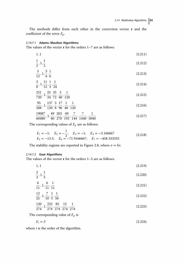
The methods differ from each other in the correction vector r and thecoefficient of the error Ep.

2.14.7.1 Adams–Moulton AlgorithmsThe values of the vector r for the orders 1–7 are as follows:

1; 1 (2.211)

12; 1;

12

(2.212)

512

; 1;34;16

(2.213)

38; 1;

1112

;13;124

(2.214)

251720

; 1;2524

;3572

;540

;1120

(2.215)

95288

; 1;137120

;58;1796

;140

;1

120(2.216)

1908760480

; 1;4940

;203270

;49192

;7

144;

71440

;1

5040(2.217)

The corresponding values of Ep are as follows:

E1 � �1; E2 � � 12; E3 � �1; E4 � �3:166667

E5 � �13:5; E6 � �71:9166667; E7 � �458:333333 (2.218)

The stability regions are reported in Figure 2.8, where σ � hλ.

2.14.7.2 Gear AlgorithmsThe values of the vector r for the orders 1–5 are as follows:

1; 1 (2.219)

23; 1;

13

(2.220)

611

; 1;611

;111

(2.221)

1225

; 1;710

;15;150

(2.222)

120274

; 1;225274

;85274

;15274

;1274

(2.223)

The corresponding value of Ep is

Ei � i! (2.224)

where i is the order of the algorithm.


The Gear algorithms have a local error about three times larger than the corre-sponding algorithms of the Adams–Moulton family.

The stability regions are reported in Figure 2.9, where σ � hλ.

The Gear algorithms are stable for stiff problems, whereas the Adams–Moultonare unstable with orders larger than 2.

2.14.8

Nonlinear System Solution

All the multivalue algorithms that we consider are implicit since they are theonly stable algorithms.It is hence necessary to deal with the problem of the solution of the nonlinear

system:

hy´ � z1 � v1 � b � hf z0; tn�1� � � hf v0 � r0b; tn�1� � (2.225)

with respect to the unknowns b.

Figure 2.8 Stability regions for the family of Adams–Moulton algorithms.


For example, in the case of the fourth-order Adams–Moulton method, wehave to solve the nonlinear system:

v1 � b � hf v0 � 38b; tn�1

(2.226)

There are two possibilities:

1) Use an iterative substitution method2) Use a version of the Newton method to solve nonlinear systems (see Vol.

3, Buzzi-Ferraris and Manenti, 2014)

For reasons that will be explained in due course, a substitution iterativemethod is adopted when the system to be solved is nonstiff and, in this case, thealgorithm adopted belongs to the Adams–Moulton family. Conversely, in stiffproblems, the nonlinear system is solved using the Newton method and thealgorithm belongs to the Gear family.

Figure 2.9 Stability regions for the family of Gear algorithms.


2.15Multivalue Algorithms for Nonstiff Problems

The alternative of solving the nonlinear system iteratively with a substitutionmethod leads to a multivalue version of the traditional predictor–correctormethod of the multistep algorithms.

The predictor–corrector method takes its name from an application of anexplicit algorithm (predictor) followed by an implicit algorithm (corrector of theprevision).

Since the method is applied to a system in the special form (2.225), the correc-tion can be obtained explicitly and, if necessary, iterated.

In the current terminology for multistep methods, the use of the explicit methodis denoted as P (prediction), the calculation of the functions f with E (evaluation),and the correction obtained by means of an implicit method with C (correction).

Then, if we calculate a single value of the functions f and a single correction,the method is called PEC; if the correction is used to calculate a new value of f ,the method is called PECE and then the PECEC, PECECE, and so on. In thisprocedure, it is opportune that the order of the two algorithms and the familywhich they belong to are the same.For example, in the case of the third-order multistep algorithm of the family of

explicit Adams–Bashforth methods and of implicit Adams–Moulton methods,the iterations are as follows:

� Prediction: y 0� �n�1 � yn � h

1223f yn; tn� � � 16f yn�1; tn�1

� � � 5f yn�2; tn�2� ��

� Evaluation: f y i� �n�1; tn�1

� �; i � 0; 1; . . .

� Correction: y i�1� �n�1 � yn � h

125f y i� �

n�1; tn�1� �

� 8f yn; tn� � � f yn�1; tn�1

� �h iIn the equivalent situation of the multivalue methods, the vector v is used as

predictor and the vector b as corrector obtained iteratively from the relation

b i�1� � � hf v0 � r0b i� �; tn�1� � � v1 (2.227)

For example, the method applied to the fourth-order multivalue Adams–Moulton algorithm consists of iterating the equation:

b i�1� � � hf v0 � 38b i� �; tn�1

� v1

starting from b 0� � � 0.Once a satisfactory vector b has been obtained, it is used to calculate the

Nordsieck vector at the n � 1� �th point.


In modern applications of this strategy, the number of iterations is limited (max-imum two or three); an accurate solution of the system (2.225) is unnecessary,although certain controls are performed on the effective convergence to thesolution. It is worth understanding the reasons and the consequences behindthis choice.

In a dedicated book (Vol. 3, Buzzi-Ferraris and Manenti, 2014), we show thatsubstitution methods rarely converge rapidly to the solution of a nonlinear sys-tem. If we need to accurately solve a system (we will see soon that this isrequired for stiff problems), it is preferable to use a variant of the Newtonmethod to achieve a faster convergence and also for another more importantreason to be explained later.

If the iterations are not fully accomplished, the system (2.225) is not accuratelysolved and the resulting algorithm is an explicit algorithm (even though compu-tationally heavy), which does not have the stability features of the implicitmethod used in the iterations.

For example, the backward Euler is strongly A-stable. Nevertheless, if thevalue of yn�1 is calculated by applying iteratively and with a limited numberof iterations the relation y i�1� �

n�1 � yn � hf y i� �n�1; tn�1

� �, where y 0� �

n�1 was calcu-lated using the forward Euler method, the method can become unstable.It is evident that in the case of nonstiff problems, the selection to waste no

calculations to search for an accurate convergence for the implicit method isreasonable since we do not need an extremely stable method in this case.We can ask ourselves why in the case of stiff problems it is unsuitable to

achieve the convergence of the iterative procedure using an adequate number ofiterations. In such a way, the method would be really implicit and, if it belongs tothe Gear family, it would be good for solving stiff problems.

If we are handling a stiff problem and we select a good algorithm to solvethis type of problems, we could use a large integration step, but by adoptinga substitution method to solve the nonlinear system, we are forced to use anextremely small integration step to avoid the iterations (2.227) diverging fromthe solution.

To understand this crucial point, we have to see how the substitution methodbehaves when applied to the reference equation. In this case, the iterations(2.227) become

b i�1� � � hλr0bi� � � hλv0 � v1 (2.228)

which are of the type

b i�1� � � mb i� � � a (2.229)

2.15 Multivalue Algorithms for Nonstiff Problems 89

As already discussed in a previous book (Buzzi-Ferraris and Manenti, 2010a),the iterations converge to the solution only if it results in

mj j < 1 (2.230)

and hence

hλr0j j < 1 (2.231)

Otherwise, the iterations diverge even though the value of the first guess is veryclose to the solution.For example, with the values λ � �1000; r0 � 1 (backward Euler method),

h � 0:01; v0 � 1; v1 � 1, the system (2.174) applied to the reference equation(2.31) becomes b � �10b � 11, with solution b � �1. By applying the substitu-tion method, we obtain the iterative formula b i�1� � � �10b i� � � 11, which divergeseven though we start from a very good guess. For example, if b 0� � � �1:001, thefollowing values of b are obtained: �98:99995, �11, 0:0000467, �11:01, 99:005,�1000:1, and so on.

The convergence radius of the substitution method is similar to the one requiredfor stability in an explicit method and is related to the product of the integrationstep and the maximum eigenvalue of the Jacobian.

Thus, even though the implicit method adopted is very stable and allows avery large integration step, we are still forced to strongly reduce the integrationstep to prevent the substitution method from diverging.

Since the predictor–corrector method is particularly suitable (when it works) interms of computational times and memory allocation (it does not need to storethe Jacobian), it is used with nonstiff problems and with algorithms that are notgood at solving stiff problems, but with better accuracy features (usually theAdams–Moulton methods are adopted).

2.16Multivalue Algorithms for Stiff Problems

The predictor–corrector method cannot solve the nonlinear system (2.225)when the problem is stiff. In this case, it is mandatory to use Newton’s method.Generally speaking, the system

v1 � b � hf v0 � r0b; tn�1� � � 0 (2.232)

can be solved with respect to b with one of the techniques valid for the nonlinearsystems (see Buzzi-Ferraris and Manenti, 2014).

In practice, it is unsuitable to use a generic program for the solution of this non-linear system, since the system (2.232) has certain special features.


This nonlinear system is special for several reasons:

1) The prediction v can be accurate enough to make the Newton methodconvergent. In fact, if the integration step h ! 0, the elements v0 and v1tend toward the elements z0 � yn and z1 � hyn � hf yn; tn

� �. Thus, as

h ! 0, the correction b ! 0. For this reason, no alternatives are usuallyadopted to force the convergence in spite of the Newton method: If anyproblem arises in the solution of the system, the integration step is simplydecreased.

The convergence of the Newton method is only indirectly related to the integra-tion step through the prediction v. If the prediction is satisfactory, the Newtonmethod can also converge with very large integration steps.This is no longer true for the substitution method that converges only when

the integration step is small for stiff problems, independent of the accuracy ofthe prediction.

The Newton method applied to the reference equation becomes

1 � hr0λ� �d � � b � hr0λb � hλv0 � v1� � (2.233)

Since in this case the equation to be zeroed to get the value b is linear, theNewton method converges in a single iteration independent of the valuesof v0; v1; λ; h.For example, taking into consideration the same values of the previous

example, λ � �1000; r0 � 1 (backward Euler method), h � 0:01; v0 � 1;v1 � 1, the relation (2.233) becomes d � � b � 10b � 11� �=11. Ifb � �1:001, it results in d � 0:001, hence the method converges in 1iteration.Obviously, the integration step influences the accuracy of the algorithm

used for the integration of the system in both the cases of the substitutionmethod and the Newton method for calculating the correction b.

2) When the nonlinear system is in the special form (2.225), the Jacobian ofthe same system, which we need for the solution through the Newtonmethod, is

G � I � hr0J (2.234)

and can be obtained immediately if the Jacobian J of the differential systemf is known. In such a case, the Newton method requires the solution of thelinear system:

Gd i� � � I � hr0J� �d i� � � �v1 � b i� � � hf v0 � r0bi� �; tn�1

� �(2.235)

from which calculate the new correction:

b i�1� � � b i� � � d i� � (2.236)

2.16 Multivalue Algorithms for Stiff Problems 91

During these iterations, the Jacobians of the differential system, J, and the non-linear system, G, are also kept constant; therefore, the same factorization is usedfor the overall procedure.

3) At each integration step, the linear system (2.235) must be solved. In theprograms that implement these methods, the matrix G is usually calculatedand then factorized each time we modify either the Jacobian J or the inte-gration step h or the order of the algorithm (r0 is modified). Once thematrix of the linearized system is factorized, the same factorization is usedfor several loops.

4) Usually it is not opportune to calculate the Jacobian J at each iteration(particularly for large-dimension problems). Rather it should be done onlywhen there are convergence problems in the system solution. When J ismodified, the matrix G must also be updated and refactorized.

5) The nonlinear system (2.225) is special with respect to the system thatwe would obtain if the differential system were not in the specialform (2.1).

Only in the special case considered here, by decreasing the integration step h weare certain we can solve the linear system related to the Newton method withoutencountering any numerical problem. In fact, in this case, the matrix G tends tothe identity matrix I.

In the general case, we can have some numerical problems in the solu-tion of the linear system related to the Newton method, when h ! 0. Forexample, if the system of differential equations is in the form

Ay´ � f y; t� � (2.237)

the matrix G becomes

G � A � hr0J (2.238)

While h ! 0, some numerical problems may arise if the matrix A issingular (differential–algebraic systems). For this reason, in the generalcase, we cannot force convergence by simply decreasing the integrationstep. Instead, it is necessary to use more sophisticated nonlinear systemsolution programs.

6) There is a difference with respect to the general case also in the control ofconvergence for the Newton method. In general nonlinear system solutionprograms, an iteration is usually accepted if certain norms of the vector ofresiduals are reduced.

In the special case considered here, the control on the convergence of the New-ton method is usually carried out so as to ensure an accuracy similar to or


smaller than the acceptable local error: The iterations are stopped when the cor-rection d is smaller than the tolerance accepted on the variables.

In this special case, a criterion analogous to the one proposed in Buzzi-Ferraris and Tronconi (1993) and adopted in BzzNonLinearSystem classfor a generic nonlinear system based on the decrease of a norm of the vectord from an iteration to the next one is adopted. Whereas in the general casethis criterion is rarely used, in this special case where the error on the varia-bles is known, the use of this criterion is quite spontaneous (Vol. 3, Buzzi-Ferraris and Manenti, 2014).

2.16.1

Robustness in Stiff Problems

To implement a multivalue algorithm to solve stiff problems, it is crucial to becareful about its robustness. In the following sections, the main causes that canmake a program unstable are analyzed and their respective remedies arediscussed.

2.16.1.1 Eigenvalues with a Very Large Imaginary PartThe multivalue algorithms used to solve stiff problems are the ones belonging tothe Gear family. They have a stability region that makes them good for handlingstiff problems. Looking at the Figure 2.9, we can see that certain instability prob-lems can also arise in this family of algorithms, but this happens only in the rare,but possible, case where the problem has an eigenvalue with a very large imagi-nary part, negative real part, and the order of the algorithm is particularly high.

If the integration step and the order of the method are controlled by means ofthe traditional criterion only (Section 2.14.4), it may happen that we are not con-scious of being in this situation. The order of the method can be kept high and,consequently, the integration step must be kept very small.

To prevent this serious problem, certain devices are needed:

� Decrease the integration step and also the order of the method when thereare convergence issues with the Newton method during the solution of thenonlinear system (2.232).� Check that the Nordsieck vector has decreasing elements; otherwise, reducethe order of the method.� In dubious cases, restart with the backward Euler method, which is stronglyA-stable.

2.16.1.2 Problems with Hard DiscontinuitiesThe multivalue algorithms have their strength in the collection of the previoushistory and, therefore, they allow a better approximation with respect to theone-step methods.


This strength can also become a weakness: If functions have certain discontinu-ities, the memory of past calculations plays against the multivalue methods.

Let us consider the reference equation (2.31) and suppose that λ suddenlychanges λ1 ! λ2 in correspondence with an instant t* (see Figure 2.10).The correction needed is given by the relation

v1 � b � hλv0 � hλr0b

Therefore, an integration step h of the order of 1=λ2 is required for b to be suffi-ciently small. If λ2 is very different from λ1, the integration step must shrink toprohibitively small values in order to have a sufficiently small b.When the step must be suddenly reduced to very small values during integra-

tion, it is useful to reinitialize the problem. By doing so, we enjoy the followingadvantages: The backward Euler method, strongly A-stable, is used and thememory of the step that generates the numerical disturbance is lost as well.

2.16.1.3 Variable ConstraintsIn many practical problems, some integration variables have constraints thatmust be satisfied to prevent physical inconsistencies or numerical problems. Forexample, in an equation like

y´ � ffiffiffiy

p

the value of y must be nonnegative.In certain situations, it is necessary to constrain some variables to prevent any

system ill-conditioning. For example, the equation

y´ � �1000y2is well conditioned if y > 0, since f y < 0, but it becomes ill-conditioned wheny < 0. In such a case, the result is

f y � �2000y > 0

y

t

1λ

2λ

n−1t nt

Corrector

Predictor

Figure 2.10 Sudden change in the value of λ.


In this situation, it is preferable not to force the user to attempt to prevent thisissue. Actually, the user could intervene as follows:

� By drastically decreasing the tolerances on the variables.� By modifying the system; for example, forcing the variable within the con-straints when they are violated.

In the former case, the number of calculations is pointlessly increased andoften the problem remains unsolved. In the latter case, a discontinuity is insertedinto the system and the number of calculations dramatically increases in theneighborhood of this point.

To make the program robust, the presence of constraints needs to be managedwithin the integration program itself.

This can be done by transforming the ODE problem into a DAE problem,where the algebraic equations that replace an even number of differential equa-tions are the constraints that are going to be violated (see Chapter 4).

2.16.2

Efficiency in Stiff Problems

To implement a multivalue algorithm for solving stiff problems, it is essential totake great care regarding efficiency. The key point with stiff problems is the solu-tion of the nonlinear system (2.232):

v1 � b � hf v0 � r0b; tn�1� � � 0

through the Newton method, which requires in turn the iterative solution of thelinear system (2.235):

Gd i� � � I � hr0J� �d i� � � �v1 � b i� � � hf v0 � r0bi� �; tn�1

� �Specifically, there are four main important issues:

� When to factorize the matrix of the linearized system G� How to factorize the matrix of the linear system G� When to update the Jacobian J� How to update the Jacobian J

2.16.2.1 When to Factorize the Matrix GIn the oldest programs for solving stiff problems, a single matrix was used: Sucha matrix contained the Jacobian J at the beginning and it was replaced by G.Finally, the same memory allocation was used to factorize the matrix G.

Memory allocation is saved by using this strategy since a single matrix is used forall the operations.


If you substitute the Jacobian J with other matrices, it is necessary to calculate iteach time we need to refactorize the matrix G.

As we will see later, in most real problems, the main computational effort (or alarge part of it) is due to the filling of the Jacobian J. For this reason, the modernprograms use two distinct matrices: the first to collect J and the second to collectG and next its factorization.The matrix G must be calculated and then factorized each time we modify

either the Jacobian J or the integration step h or the order of the algorithm (r0 ismodified). For this reason, it is important to preserve where possible the order ofthe method and the integration step.

2.16.2.2 How to Factorize the Matrix GIn many practical problems, the Jacobian J and thus the matrix G are sparse andstructured. It is therefore indispensable to use a dedicated factorization thatexploits such a feature.Since the user may not be familiar with all the possible factorization forms, a

good program must contain an automatic selection of the most appealingfactorization.

When several processors are available and parallel computing can be exploited,it is possible to boost the performance of the factorization of matrix G.

2.16.2.3 When to Update the Jacobian JIn most practical problems, the Jacobian J must be numerically evaluated and, todo so, we need as many system calls as the number of elements of the vector y ifthe Jacobian is dense.

We noted that it is preferable to preserve the Jacobian for several iterations,unless it compromises the convergence of the Newton method in the solution ofthe nonlinear system (2.232).

For this reason, the implicit algorithms, which seem to be less efficient than thesemi-implicit ones, are the best choice. In fact, the semi-implicit algorithms can-not use this strategy since the Jacobian is within their own formulation, whereasthe implicit algorithms use the Jacobian only for the convergence of the Newtonmethod.

The Jacobian must be updated when the convergence efficiency of theNewton method decays. It is usually recalculated after an assigned numberof iterations. In such a case, it is preferable to link this update to the prob-lem dimension. In fact, the advantages to keeping the Jacobian constantincrease with the size of the problem. With small-dimension problems, it canbe disadvantageous to keep the Jacobian constant since the increase in thenumber of iterations can be larger than the computations saved to decreasethe number of Jacobian calculations.


The following additional check has been inserted in the BzzOdeStiff class toverify the Jacobian accuracy.

Since at the generic iteration, the values of f i, J, yi�1 � yi are known, it is there-fore possible to evaluate

f*i�1 � f i � J yi�1 � yi� � � @f i

@th (2.239)

and compare it with the known f i�1. In case the two values are too different, theJacobian has to be updated.

2.16.2.4 How to Update the Jacobian JWhen the number of equations and variables is quite large, each equation oftendepends on a reduced set of variables. It is necessary to exploit the sparsity of theJacobian matrix so as to reduce memory allocation while saving CPU time. Inparticular, the following expedients are essential:

1) The solution of the system (2.219) should be achieved by the method thatbest exploits Jacobian sparsity and structure.

2) If the Jacobian does not have a specific structure that can be directlyexploited, it is worthwhile rearranging both the variables and equations toreduce CPU effort and the memory allocation required by the factorizationof the Jacobian matrix.

3) The null Jacobian elements should not be evaluated. This happens auto-matically if the Jacobian is analytically evaluated. Conversely, whenever theJacobian matrix is numerically approximated, the computation

J ik � f j xi � hkek� � � f j xi� �hk

(2.240)

should be avoided if it is known a priori that f j xi � hkek� � � f j xi� �.4) If the Jacobian is evaluated numerically, it is not convenient to increment

variables one at a time and to perform a call to the nonlinear system.

Buzzi-Ferraris and Manenti (2014, Vol. 3) have shown that the Jacobian of anonlinear system can be calculated by simultaneously varying several variableswhen the Jacobian is sparse. If Equation 2.240 is adopted to evaluate a Jacobianmatrix, which is supposed to be full, then the vector ek is the null array exceptfor position k where the element is equal to 1. In this case, the system is called Ntimes to evaluate the derivatives of the functions with respect to the N variables.Consider the sparse Jacobian matrix shown in Figure 2.11, where the symbol ×represents a nonzero element.


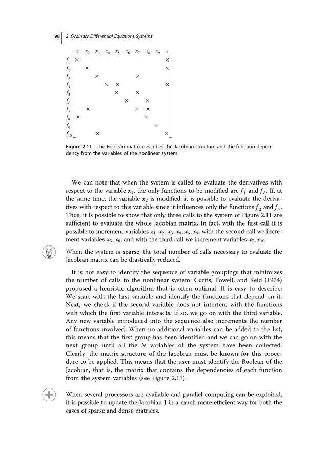
We can note that when the system is called to evaluate the derivatives withrespect to the variable x1, the only functions to be modified are f 1 and f 8. If, atthe same time, the variable x2 is modified, it is possible to evaluate the deriva-tives with respect to this variable since it influences only the functions f 2 and f 7.Thus, it is possible to show that only three calls to the system of Figure 2.11 aresufficient to evaluate the whole Jacobian matrix. In fact, with the first call it ispossible to increment variables x1; x2; x3; x4; x6; x9; with the second call we incre-ment variables x5; x8; and with the third call we increment variables x7; x10.

When the system is sparse, the total number of calls necessary to evaluate theJacobian matrix can be drastically reduced.

It is not easy to identify the sequence of variable groupings that minimizesthe number of calls to the nonlinear system. Curtis, Powell, and Reid (1974)proposed a heuristic algorithm that is often optimal. It is easy to describe:We start with the first variable and identify the functions that depend on it.Next, we check if the second variable does not interfere with the functionswith which the first variable interacts. If so, we go on with the third variable.Any new variable introduced into the sequence also increments the numberof functions involved. When no additional variables can be added to the list,this means that the first group has been identified and we can go on with thenext group until all the N variables of the system have been collected.Clearly, the matrix structure of the Jacobian must be known for this proce-dure to be applied. This means that the user must identify the Boolean of theJacobian, that is, the matrix that contains the dependencies of each functionfrom the system variables (see Figure 2.11).

When several processors are available and parallel computing can be exploited,it is possible to update the Jacobian J in a much more efficient way for both thecases of sparse and dense matrices.

987654321

1

2

3

4

5

6

7

8

9

10

x xxxxxxxxx

f

f

f

f

f

f

f

f

f

f

××

××

××

× ××

××

××

×××

××

×

× ×

Figure 2.11 The Boolean matrix describes the Jacobian structure and the function depen-dency from the variables of the nonlinear system.


2.17Multivalue Classes in BzzMath Library

The following classes, which are based on multivalue algorithms, are imple-mented in the BzzMath library.

For the nonstiff problems, based on multivalue algorithms of the Adams–Moulton family:

BzzOdeNonStiffBzzOdeNonStiffObject

For the stiff problems, based on multivalue algorithms of the Gear family:

BzzOdeStiffBzzOdeSparseStiffBzzOdeStiffObjectBzzOdeSparseStiffObject

The BzzOdeNonStiff and BzzOdeStiff classes have two constructors:

BzzOdeNonStiff o1(y0,t0,OdeSample);BzzOdeNonStiff o2;o2(y0,t0,OdeSample);

The first constructor has the following in its argument:

� The BzzVector y0, which contains the initial values of y, y0. If a singleequation is to be integrated, the vector has dimension 1.� The double t0, value of t0 (initial value of the independent variable).� The name of the function in which the system is calculated.

The second constructor is the default constructor. Once defined as anobject of the class BzzOdeNonStiff or BzzOdeStiff, it can be initializedusing the overlapped operator () with the same argument as the previousconstructor.Using the operator (), it is possible to reinitialize an object with a new start-

ing point and/or with the name of the same function or of a different functionalso where a novel system to be integrated is implemented.The user must provide the prototype declaration for the function f y; t� �,

where the system is calculated before defining an object that uses it withinthe program. The function input is the vector y and the corresponding t,which are managed by the object. The output is the vector f . For efficiencyreasons and for greater ease of use, the vectors y and f are both BzzVector

references.


2.17 Multivalue Classes in BzzMath Library 99

Example 2.2

Integrate the following two systems:y1 � �0:1y1 � 49:9y2y2 � �50y2y3 � 70y2 � 120y3

in the range t � 0; 1� � and initial conditions y01 2; 1; 2f g and

y1 � 1y2

y2 � � 1y1

in the range t � 0; 10� � and initial conditions y01 1; 1f g.The program is


//prototypevoid OdeNonStiff1(BzzVector &y,double t,

BzzVector &f);void OdeNonStiff2(BzzVector &y,double t,


{BzzVector y;BzzVector y01(3,2.,1.,2.);BzzOdeNonStiff o(y01,0.,OdeNonStiff1);y = o(1.);o.BzzPrint(“Non Stiff1 Results”);BzzVector y02(2,1.,1.);o(y02,0.,OdeNonStiff2);y = o(10.);o.BzzPrint(“Non Stiff2 Results”);}

void OdeNonStiff1(BzzVector &y,double t,BzzVector &f){f[1] =-.1 * y[1] - 49.9 * y[2];f[2] = -50. * y[2];f[3] = 70. * y[2] - 120. * y[3];}

void OdeNonStiff2(BzzVector &y,double t,BzzVector &f){f[1] = 1./y[2];f[2] = -1./y[1];}


In the following example, the difference between an algorithm for stiff problemsand one for nonstiff problems is highlighted.

Example 2.3

Integrate the following stiff system:

y1 � �r1 � r2y2 � r1 � r2 � r3y3 � r3

r1 � 0:04y1

r2 � 104y2y3

r3 � 3 � 1014y22with initial conditions y1 0� � � 1; y2 0� � � 0; y3 0� � � 0, using a program based onan algorithm incapable of tackling stiff problems and compare the results withthe solution obtained with a proper algorithm.The program is


//prototypevoid OdeExample3(BzzVector &y,double t,


{BzzVector y0(3,1.,0.,0.),y;double tOut;tOut = 0.01;BzzOdeNonStiff on(y0,0.,OdeExample3);y = on(tOut);on.BzzPrint(“Non Stiff Results for tOut = 0.01”);BzzOdeStiff of(y0,0.,OdeExample3);y = of(tOut);of.BzzPrint(“Stiff Results for tOut = 0.01”);tOut = 100.;y = of(tOut);of.BzzPrint(“Stiff Results for tOut = 100.”);}

void OdeExample3(BzzVector &y,double t,BzzVector &f){double r1,r2,r3;r1 = 0.04 * y[1];


r2 = 1.e4 * y[2] * y[3];r3 = 3.e14 * y[2] * y[2];f[1] = -r1 + r2;f[2] = r1 - r2 - r3;f[3] = r3;}

The object on of the BzzOdeNonStiff class needs 121 199 evaluations of thesystem to perform the integration between 0 and 0.01. In addition, the numberof calculations is too large for the integration between 0 and 100.The object of of the BzzOdeStiff class, which can tackle stiff problems,

needs 115 evaluations of the system for integration between 0 and 0.01, whereas271 evaluations are needed for integration between 0 and 100.The BzzOdeNonStiffObject and BzzOdeStiffObject classes are differ-

ent from the previous BzzOdeNonStiff and BzzOdeStiff classes becausetheir objects are initialized with an object rather than the name of the function.Consider the previous example OdeNonStiff1. Now the program is

BzzVector y0(3,2.,1.,2.),y;BzzVector data(5,-0.1,-49.9,-50.,70.,-120.);MyOdeSystemObject odeSampleObject(data);BzzOdeNonStiffObject o(y0,0., &odeSampleObject);o(y0,t0, &odeSampleObject);y = o(1.);o.BzzPrint(“Results”);

The object odeSampleObject must belong to a class, MyOdeSystemOb-

ject, created by the user and derived from the class BzzOdeSystemObject.For example:

class MyOdeSystemObject : public BzzOdeSystemObject{

private:BzzVector data;

public:MyOdeSystemObject(BzzVector &dat)

{data = dat;}virtual void GetSystemFunctions(BzzVector &y,

double t,BzzVector &f);virtual void ObjectBzzPrint(void);

};

void MyOdeSystemObject::ObjectBzzPrint(void){::BzzPrint(“\n\nObject Print”);data.BzzPrint(“Data”);}


void MyOdeSystemObject::GetSystemFunctions(BzzVector &y,double t,BzzVector &f)

{f[1] = data[1] * y[1] + data[2] * y[2];f[2] = data[3] * y[2];f[3] = data[4] * y[2] + data[5] * y[3];}

Note that the user must provide

GetSystemFunctionsObjectBzzPrint

The former is used to define the system; the latter is used to personalize theprintout of results.The class must contain a constructor to initialize the data for the proper use of

the two functions above. Global variables are unnecessary in this case.An object of all the previous classes, as it is defined, automatically receives a

default value for the tolerances of the absolute (1.e-10) and relative (1.e-6)

errors on the variables yi.It is possible to modify the default values of such tolerances using the func-

tions SetTolAbs and SetTolRel, which accept as their argument both a singlevalue for all the variables and a BzzVector to assign a special tolerance to eachvariable:

BzzVector tolAbs(3,1.e-3,1.e-4,1.e-5);BzzVector tolRel(3,.001,.0001,.00001);double tolA = 1.e-5; // default 1.e-10double tolR = 1.e-4; // default 1.e-6o1.SetTolAbs(tolAbs);o2.SetTolRel(tolRel);o3.SetTolAbs(tolA);o4.SetTolRel(tolR);

The objects of these classes not only remember their history but also exploit theproperty of multivalue methods to maintain the optimal integration step distinctfrom the user requests.

If the user uses the object for progressively increased tOut, the integration isnot performed by starting each time from t0, but from the value of t achievedin the previous iteration with an already estimated integration step. Moreover,the integration step that is really adopted generally overcomes the value of tOut

for which the vector y is required. If we want to prevent this integration stepgoing beyond an assigned value, just add that value as an argument of the opera-tor (). For example:

y = o(tOut,tCritic);


Objects in these classes can use some special functions:

� SetMinimumConstraints� SetMaximumConstraints

These functions provide bounds to the integration variables y. If one of themachieves the bound, the object automatically considers that relation as an alge-braic equation by preventing any violation.Example:

BzzVector yMin(numVariables);BzzVector yMax(numVariables);yMax = 1.;o.SetMinimumConstraints(yMin);o.SetMaximumConstraints(yMax);

� StepPrint

There are three versions of this function. They allow a printout onto aselected file of the values of the variables t and y in correspondence with themesh points used during the integration.The first function requires only the name of the file. All the values of the

variables y are printed out.Example:

o.StepPrint(“RESULTS.TXT”);

The second version requires as the argument both the name of the fileand a BzzVectorInt where the indices of the variables to be printed areprovided. It is also possible to add a comment.Example:

BzzVectorInt lv(2);lv[1] = 1; lv[2] = 3;o.StepPrint(“RESULTS2.TXT”,lv,”Variables 1 and 3”);

The third version requires as the argument the name of a function pro-vided by the user indicating what has to be printed.Example:

o.StepPrint(MyPrint);

Such a function is automatically invoked at each integration step and withthe appropriate value of t and its corresponding y and must have the follow-ing argument as well:

void MyPrint(BzzVector &y,double t);

� StepDebug


This function has several versions. The simplest one requires just thename of the file used for printing the relevant information such as the valueof t, the integration step, the variable with maximum error, and the value ofthe error.Example:

o.StepDebug(“debug.txt”);

� GetInitAndEndTimeStep

This function allows us to know the values at the beginning and at the endof each integration step actually used.

Example:

o.GetInitAndEndTimeStep(&tInitStep, &tEndStep);

� GetTimeInMeshPoint� GetYInMeshPoint� GetY1InMeshPoint

These functions allow us to know t, y, and y´ for each integration step.

Additional examples and tests of the use of

BzzOdeNonStiff,BzzOdeNonStiffObject,

BzzOdeStiff, andBzzOdeStiffObject classes can be found in


directory and

OdeNonStiffOdeNonStiffObjectOdeStiffOdeStiffObjectOdeNonStiffTestsOdeStiffTests

subdirectories in BzzMath7.zip file available at the web site:http://www.chem.polimi.it/homes/gbuzzi.

The objects of the classes BzzOdeSparseStiff and BzzOdeSparseStif-

fObject exploit the devices broached in Section 2.16.2.4 when the Jacobianmatrix is sparse.

These classes use different constructors to indicate the kind of Jacobian struc-ture. The most important cases are as follows:



� Sparse and unstructured JacobianIn this case, the user must provide the indices of the rows and columns

where the Jacobian is nonzero. This can be done in two ways: either usingtwo BzzVectorInt containing the row and column indices for each non-zero element or using an object of the BzzMatrixCoefficientsExis-

tence class.Using the first way, we have

BzzOdeSparseStiff o;BzzVectorInt r(numElements,1,2,2, . . . );BzzVectorInt c(numElements,1,2,4, . . . );o(y0,t0,OdeSparseGeneric, &r, &c);

whereas using the second way, we have

BzzMatrixCoefficientsExistence Je(300,300);Je(1,1),Je(1,2),Je(2,1),Je(2,2),Je(2,3), . . . . . . ;BzzOdeSparseStiff o(y0,t0,OdeSparseGeneric, &Je);

The latter alternative was adopted in release 6 of BzzMath library and is nowconsidered obsolete since the new way adopts a more efficient linear systemsolver.

� Band JacobianIn this case, only the upper and lower band values need to be indicated.

BzzOdeSparseStiff o(y0,t0,OdeBand,5,7);

� Tridiagonal blocks JacobianIn this case, only the size of the blocks on the three diagonals needs to be

indicated.

BzzOdeSparseStiff o(y0,t0,OdeTridiagonalBlock,4);

Additional examples and tests of the use of BzzOdeSparseStiff, and BzzO-

deSparseStiffObject classes can be found in


directory and

OdeSparseStiffOdeSparseStiffObject




2.18Extrapolation Methods

The methods from this family use extrapolations in the forms considered inBuzzi-Ferraris and Manenti (2010b). In the case of nonstiff differential equations,the most common extrapolation is as follows.

The algorithm usually adopted to prepare the points for the extrapolation,obtained by varying h, is a variant of the central point method proposed byGragg (Stoer and Bulirsch, 1983), while the extrapolation for h ! 0 is performedeither with the Richardson method applied to polynomials or the Bulirsch–Stoer(Stoer and Bulirsch, 1983) method applied to rational functions.

The central point method:

yn�1 � yn�1 � 2hf yn; tn� �

; y0 � y t0� �; n � 2; . . . (2.241)

has two serious problems:

1) It has a side solution, which is unstable and oscillating (as demonstrated inthe discussion on the stability of the multistep algorithms).

2) It requires the value of y in t1 to be known.

Nevertheless, it still has the following advantage.

The formula to calculate its local error is constituted by even powers of h only.

Gragg modified the middle point method to preserve the features of the localerror, but reducing the influence of the side solution and, at the same time, mak-ing the method self-consistent.The Gragg method consists of the following equations:

y1 � y0 � hN f y0; t0� �

; y0 � y t0� � (2.242)

yn�1 � yn�1 � 2hN f yn; tn� �

; n � 1; 2; . . . ;N N even number� � (2.243)

yhNF tF � tN� � � yN � yN�1 � hN f yN ; tN� �

2(2.244)

To integrate from t0 to tF , we use the integration step:

hN � tF � t0N

N even number� � (2.245)

tF � tN � t0 � NhN (2.246)

The method then can proceed as if solving the initial value problem:

y´ � f y; t� �; y tF� � � yF (2.247)

2.18 Extrapolation Methods 107

This is the modified middle point Gragg method. It is a modified middle pointbecause of the following:

1) The first step uses the relation (2.242) like the Euler forward method.2) The last step uses the relation (2.244) to reduce the influence of the para-

site solution.

If the method is used with the extrapolation procedure, it is iterated with dif-ferent values of hN (different values for the number of steps N) so as to obtain abetter value of yF .There are different strategies for the selection of the series of N . Years ago, the

Romberg series was used: 2, 4, 8, 16, . . . . Nowadays, the following series is pre-ferred: 2, 4, 6, 8, 12, 16, 24, . . . , since it induces a less rapid decrease in the integra-tion step and, consequently, a slower increase in the number of the required steps.By denoting with yhNi;F the ith component of the vector yF obtained for a particular

value of hN , Gragg demonstrated that the error in tF can be expressed as follows:

yhNi;F � yi tF� � � C1h2N � C2h

4N � C3h

6N � ∙ ∙ ∙ (2.248)

Once the value of yhNi;F is calculated for different hN , an extrapolation for h � 0is performed. For the extrapolation, we can use a polynomial approximation withthe Neville algorithm, which is equivalent to the Richardson extrapolation forthis specific case, or better still, a rational function using the Bulirsch–Stoeralgorithm. The convergence of the method can be assessed by comparing thetwo different values of the extrapolation.

The procedure, when it works, is very efficient: It needs a smaller overall amountof calculations of the system f for any alternative.

Unfortunately, however, for Gragg variant, there is always the chance of encoun-tering instability phenomena due to the side solution.

Clearly, the Gragg algorithm cannot be used for stiff problems.

If the problem is stiff, it is necessary to use an A-stable or, better still, strongly A-stable algorithm such as the backward Euler method (2.12) or the Cash method.

In the BzzMath library, these algorithms have not been implemented in dedi-cated classes.

2.19Some Caveats

Caveat No. 1To solve differential equations, it is essential to have information regarding thephysical system.


The user must be able to assess the qualitative behavior of the solution. Neverassume that a solution is good only because it was obtained using a goodprogram.

Caveat No. 2There are different ways of transforming a high-order differential system into afirst-order system. It is opportune not to limit the selection to the simplest wayof introducing a new variable and imposing it as the first derivative of an existingvariable. For instance, the equation

y´´ � G t� �y´ � F t� � (2.249)

is transformed into the system:

y1 � y2

y2 � F t� � � G t� �y2(2.250)

It is mandatory to check that the behavior of the new variables is not irregularand that they are in line with the physics of the system.

It could also be advantageous to insert other elements dictated by the physicalsystem, such as functions of the independent variable t, to smoothen the trendsof the new variables.

Caveat No. 3A bit of confusion may arise between stiff and nonstiff problems and well- andill-conditioned systems. For example, the equation

y´´ � 100y � 0 (2.251)

has the following general solution:

y � C1e�10t � C2e

10t (2.252)

This equation cannot be integrated numerically using the techniques broachedin this chapter when it is integrated with all the conditions on the left of theintegration interval, not because it is stiff (due to C1e�10t), but because it is ill-conditioned (due to C2e10t).

It is worth remarking that the equation is also ill-conditioned when it is inte-grated with all the conditions on the right of the integration interval, due to theterm C1e�10t . Conversely, it can be solved if the conditions are placed oppor-tunely at the two boundaries of the interval by means of the techniquesdescribed in Chapter 6.

Caveat No. 4The problem of the existence and uniqueness of the solution for a differentialequation system with initial conditions is not broached in this book.

2.19 Some Caveats 109

It is possible to provide examples in which there is no solution or others still inwhich the solution is not unique.

We refer our readers to specific math books on the topic.All the topics included in this volume assume that the solution is unique.

Caveat No. 5Numerical program users should be aware of the fact that some initial valueproblems do not have a unique solution.

Since a numerical program applied without this consideration could producepuzzling results, it is crucial that the user checks the solution and compares itwith the one expected from looking at the physical system.

Caveat No. 6Many algorithms that were considered valid in the past are nowadays simplyobsolete.

As in any area of numerical analysis, the effectiveness of an algorithm is nowassessed not on its efficiency but on its stability and robustness. It is pointless touse an algorithm with a theoretically very small local error if its stability region isalso very small.

For instance, it is preferable not to adopt the Milne multistep method largelyused in the past: Although it has a very small local error, it also has a veryunfavorable stability region.


3ODE: Case Studies

Examples from this chapter can be found in the Vol4_Chapter3 directory inthe WileyVol4.zip file available at the following web site:http://www.chem.polimi.it/homes/gbuzzi.

3.1Introduction

Several case studies dealing with ODE solutions are outlined in this chapter.ODEs are obtained not only from classical applications commonly used as testsbut also from real chemical engineering problems. An interesting review con-taining large-dimension problems is proposed by Byrne and Hindmarsh (1987).The CATalytic Post-Processor (CAT-PP) by Corbetta et al. (2014), which cou-ples programming and computational fluid dynamic (CFD) codes to simulatehighly diluted reactive heterogeneous systems, is selected as an industrial valida-tion case.

3.2Nonstiff Problems

The following 15 problems have been proposed by different authors and belongto the nonstiff family. They can be integrated using traditional methods:

1) Problem no. 1 (Lapidus and Seinfeld, 1971):

y´ � �yy 0� � � 1

tF � 25

The solution is

y � e�tF

111




y´ � y

y 0� � � 1

tF � 25

The solution is

y � etF


y1 � 1=y2

y2 � �1=y1y1 0� � � 1

y2 0� � � 1

tF � 10

The solution is

y1 � etF

y2 � e�tF


y1 � y2

y2 � �y1y1 0� � � 1

y2 0� � � 1

tF � 3

The solution is

y1 � sin tF� �y2 � cos tF� �


y1 � �0:1y1 � 49:9y2

y2 � �50y2y3 � 70y2 � 120y3

y1 0� � � 2

y2 0� � � 1

y3 0� � � 2

112 3 ODE: Case Studies

tF � 1

The solution is

y1 � e�0:1tF � e�50tF

y2 � e�50tF

y3 � e�50tF � e�120tF


y´ � 1 � y2

y 0� � � 0

tF � 6

The solution is

y � e2tF � 1e2tF � 1

7) Problem no. 7 (Atkinson, 1989):

y´ � 11 � t2

� 2y2

y 0� � � 0

tF � 10

The solution is

y � tF1 � t2F

8) Problem no. 8 (Atkinson, 1989):

y´ � y4

1 � y20

� �y 0� � � 1

tF � 20

The solution is

y � 201 � 19e�tF=4

9) Problem no. 9 (Kahaner, Moler, and Nash, 1989):

y´ � �10 t � 1� �yy 0� � � 1

tF � 1

The solution is

y � 148:41316

3.2 Nonstiff Problems 113

10) Problem no. 10 (Buchanan and Turner, 1992):

y´ � 5 t � 1� �yy 0� � � 5

tF � 1:25

The solution is

y � 5e2:5t2F�5tF


y´ � 1 � t2

y 0� � � 0

tF � 1:5

The solution is

y � tan tF� �12) Problem no. 12 (Buchanan and Turner, 1992):

y´ � cosπt12

� �� y

y 0� � � 50

tF � 30

The solution is

y � cos πtF=12� � � π=12� � sin πtF=12� �1 � π=12� �2 � 50 � 1

1 � π=12� �2 !

e�tF


y1 � �2y1 � y2 � e�3t

y2 � 2y1 � y2 � y3

y3 � 2y2 � 2y3 � e�3t

y1 0� � � 1

y2 0� � � 0

y3 0� � � 0

tF � 3

The solution is

y1 � �2e�tF � 4 � 2tF� �e�2tF � e�3tF

y2 � 2e�tF � 2e�2tF


y3 � 4e�tF � 6 � 4tF� �e�2tF � 2e�3tF


y1 � y2

y2 � �2y1 � 0:5y3

y3 � y4

y4 � 2y1 � 2y3 � 10 cos 2t� �y1 0� � � 0

y2 0� � � 0

y3 0� � � 0

y4 0� � � 0

tF � 20

The solution is

y2 � 53cos 2tF� � � 5

6cos tF� � � 5

2cos

ffiffiffi3

ptF

� �

y4 � � 203

cos 2tF� � � 53cos tF� � � 5 cos

ffiffiffi3

ptF

� �15) Problem no. 15 (Buchanan and Turner, 1992):

y´ � 1 � y; t < π

y´ � �5y; t � π

y 0� � � 0; tF � 5

The solution of the problem is

y � 1 � e�π� �e �5 tF�π� �� ; tF > π

The code that includes all these examples can be found in


directory and

OdeNonStiffTests

subdirectory in BzzMath7.zip file available at the web site:http://www.chem.polimi.it/homes/gbuzzi.

Table 3.1 shows a comparison of the performances of the different objectsfrom the BzzOdeNonStiff, BzzOdeRK, BzzOdeRKF, BzzOdeRKM, andBzzOdeRKS classes. The performance ratio between the Runge–Kutta (RK)methods and the Adams–Moulton (AM) method is reported in parentheses.

3.2 Nonstiff Problems 115


3.3Volterra System

The Volterra ODE system offers a simple model for the correlated population ofpredators (foxes), y2, and prey (rabbits), y1:

� An increase in the number of foxes decreases the rate at which rabbitsproliferate.� An increase of the number of rabbits increases the rate at which the foxesproliferate.

The system of equations is

y1 � 0:05 � y1 � 1 � 0:01 � y2� �

y2 � 0:1 � y2 � 0:005 � y1 � 2� � (3.1)

and has to be integrated in the range t � 0; 600� � with initial conditions y1 0� � �1500 and y2 0� � � 100.

Example 3.1

The program is

#define BZZ_COMPILER 0 // Visual C++ 6 Compiler#include “BzzMath.hpp”void BzzVolterra(BzzVector &y,

double t,BzzVector &f);

Table 3.1 Performance comparison (number of iterations) of objects of different classes; thecomparison with the AM is shown in parentheses.

Tests AM RK RKF RKM RKS

1 304 691(2.3) 509(1.7) 424(1.4) 713(2.3)2 242 1077(4.5) 803(3.3) 689(2.8) 1187(4.9)3 165 472(2.9) 419(2.5) 624(3.8) 677(4.1)4 74 175(2.4) 126(1.7) 105(1.4) 196(2.6)5 474 834(1.8) 627(1.3) 541(1.1) 930(2.0)6 124 241(1.9) 167(1.3) 204(1.6) 251(2.0)7 167 339(2.0) 249(1.5) 344(2.1) 341(2.0)8 88 164(1.9) 107(1.2) 183(2.1) 167(1.9)9 88 252(2.9) 184(2.1) 269(3.1) 263(3.0)10 90 164(1.8) 130(1.4) 234(2.6) 166(1.8)11 155 247(1.6) 137(0.9) 305(2.0) 210(1.4)12 314 987(3.1) 706(2.2) 836(2.7) 1064(3.4)13 127 340(2.7) 251(2.0) 357(2.8) 353(2.8)14 673 2624(3.9) 1941(2.9) 2049(3.0) 2691(4.0)15 216 780(3.6) 483(2.2) 444(2.1) 659(3.1)

2.6 1.9 2.3 2.8


void main(void){BzzPrint(“\n\nVolterra”);BzzVector y0(2,1500.,100.),y;double t0 = 0.,tOut = 600.;BzzOdeStiff o(y0,t0,Volterra);o.StepPrint(“Volterra.txt”);y = o(tOut);}

void Volterra(BzzVector &y,double t,BzzVector &f)

{f[1] = 0.05 * y[1] * (1. � 0.01 * y[2]);f[2] = 0.1 * y[2] * (0.005 * y[1] � 2.);}

Having inserted the statement:

o.StepPrint(“Volterra.txt”);

the program prints the entire evolution of the calculations. The plot of the twovariables is reported in Figure 3.1.

3.4Simulation of Catalytic Effects

As reported in Rice (1993), the simulation of catalytic effects is considered as anODE system. Under steady-state conditions, an ideal gas G diffuses through aflat gas film with a thickness T (Figure 3.2). A catalytic surface is placed att � T , where G undergoes the reaction G ! pU � qV . With the appropriateconstants A to F , the concentrations v and u of the reaction products V and Uare simulated as follows:

0

200

400

600

800

1000

1200

1400

1600

0 100 200 300 400 500 600

Time

Figure 3.1 Volterra system.

3.4 Simulation of Catalytic Effects 117

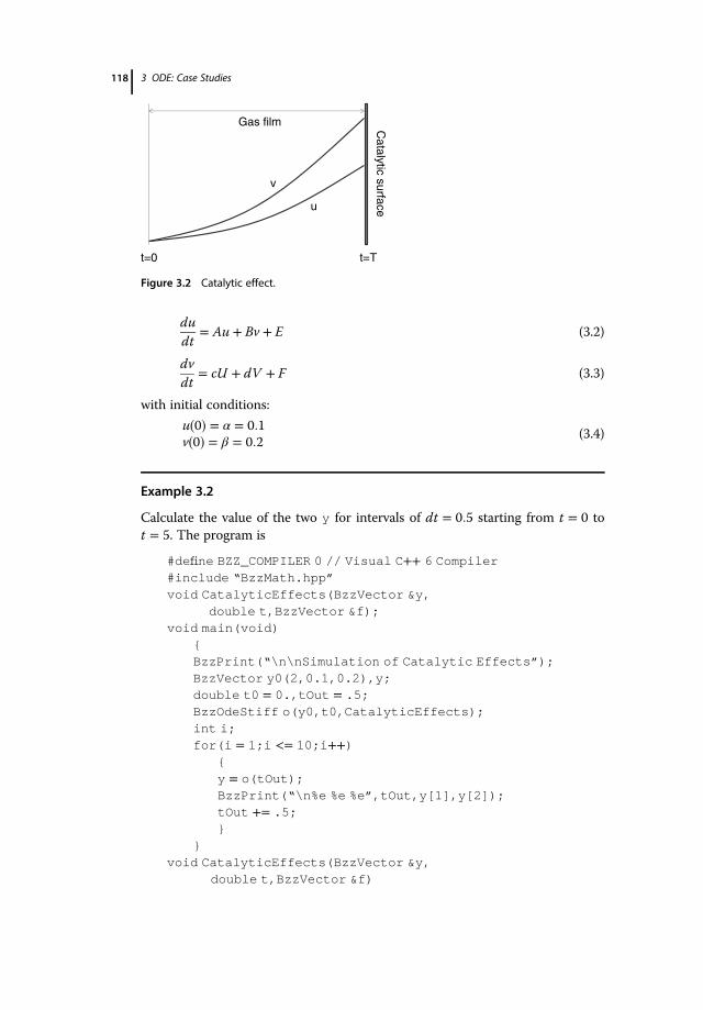
dudt

� Au � Bv � E (3.2)

dvdt

� cU � dV � F (3.3)

with initial conditions:

u 0� � � α � 0:1v 0� � � β � 0:2

(3.4)

Example 3.2

Calculate the value of the two y for intervals of dt � 0:5 starting from t � 0 tot � 5. The program is

#define BZZ_COMPILER 0 // Visual C++ 6 Compiler#include “BzzMath.hpp”void CatalyticEffects(BzzVector &y,

double t,BzzVector &f);void main(void)

{BzzPrint(“\n\nSimulation of Catalytic Effects”);BzzVector y0(2,0.1,0.2),y;double t0 = 0.,tOut = .5;BzzOdeStiff o(y0,t0,CatalyticEffects);int i;for(i = 1;i <= 10;i++)

{y = o(tOut);BzzPrint(“\n%e %e %e”,tOut,y[1],y[2]);tOut += .5;}

}void CatalyticEffects(BzzVector &y,

double t,BzzVector &f)

t=Tt=0

v

u

Catalytic surface

Gas film

Figure 3.2 Catalytic effect.


{double A = 0.5;double B = 0.1;double C = 0.3;double D = 0.4;double E = 0.1;double F = 0.2;f[1] = A * y[1] + B * y[2] + E;f[2] = C * y[1] + D * y[2] + F;}

It results in

Simulation of Catalytic Effects5.000000e-001 2.012081e-001 3.792391e-0011.000000e+000 3.428787e-001 6.180335e-0011.500000e+000 5.404321e-001 9.374602e-0012.000000e+000 8.150594e-001 1.366257e+0002.500000e+000 1.195876e+000 1.943648e+0003.000000e+000 1.722862e+000 2.723199e+0003.500000e+000 2.450902e+000 3.778106e+0004.000000e+000 3.455318e+000 5.208436e+0004.500000e+000 4.839457e+000 7.151045e+0005.000000e+000 6.745091e+000 9.793169e+000

3.5Ozone Decomposition

The system that characterizes the ozone decomposition was proposed andsolved by Bowen (Lapidus and Seinfeld, 1971):

y1 � �y1 � y1y2 � 3y298

y2 � 98 y1 � y1y2 � 3y2� �

y1 0� � � 1; y2 0� � � 0; 0 � t � 5

Example 3.3

The program is

#define BZZ_COMPILER 0 // Visual C++ 6 Compiler#include “BzzMath.hpp”void OzoneDecomposition(BzzVector &y,


3.5 Ozone Decomposition 119

{BzzPrint(“\n\nOzone Decomposition”);double t0 = 0.,tOut = 5.;BzzVector y0(2,1.,0.),y;BzzOdeStiff o(y0,t0,OzoneDecomposition);y = o(tOut);o.BzzPrint(“Results”);}

void OzoneDecomposition(BzzVector &y,double t,BzzVector &f)

{f[1] = -y[1] - y[1]*y[2] + 3./98.*y[2];f[2] = 98.*(y[1] - y[1]*y[2] - 3.*y[2]);}

It results in

Total number of system evaluations 263y in the output point: tOut = 5.000000e+000

1 5.47680688440212e-0032 1.82841997566044e-003

3.6Robertson’s Kinetic

The kinetic of Robertson (1967) is stated as follows:

r1 � 0:04y1

r2 � 104y2y3

r3 � 3 � 1010 y22

y1 � �r1 � r2

y2 � r1 � r2 � r3

y3 � r3

y1 0� � � 1; y2 0� � � 0; y3 0� � � 0; 0 � t � 4 000 000

Example 3.4

The program is

#define BZZ_COMPILER 0 // Visual C++ 6 Compiler#include “BzzMath.hpp”void RobertsonKinetic(BzzVector &y,



{BzzPrint(“\n\nRobertson Kinetic”);BzzVector y0(3,1.,0.,0.),y;double t0 = 0.,tOut = 4000000.;BzzOdeStiff o(y0,t0,RobertsonKinetic);y = o(tOut);o.BzzPrint(“Results”);BzzPause();}

void RobertsonKinetic(BzzVector &y,double t,BzzVector &f)

{double r1 = .04*y[1];double r2 = 1.e4*y[2]*y[3];double r3 = 3.e10*y[2]*y[2];f[1] = -r1 + r2;f[2] = r1 - r2 - r3;f[3] = r3;}

It results in

Total number of system evaluations 658y in the output point: tOut = 4.000000e+006

1 5.20933733411992e-0072 2.08372299191111e-0123 9.99999479064182e-001

3.7Belousov’s Reaction

Belousov’s reaction (Field and Noyes, 1974) is stated as follows:

y1 � 77:27 y2 � y1 1 � y2 � 8:375 � 10�6y1� ��

y2 � �y2 1 � y1� � � y3

� �=77:27

y3 � 0:161 y1 � y3� �

y1 0� � � 4

y2 0� � � 1:1

y3 0� � � 4

0 � t � 300

3.7 Belousov’s Reaction 121

Example 3.5

The program is

#define BZZ_COMPILER 0 // Visual C++ 6 Compiler#include “BzzMath.hpp”void BelousovReaction(BzzVector &y,


{BzzPrint(“\n\nBelousov Reaction”);BzzVector y0(3,4.,1.1,4.),y;double t0 = 0.,tOut = 300.;BzzOdeStiff o(y0,t0,BelousovReaction);y = o(tOut);o.BzzPrint(“Results”);}

void BelousovReaction(BzzVector &y,double t,BzzVector &f)

{f[1]=77.27*(y[2]+y[1]*(1.-y[2]-8.375e-6*y[1]));f[2]=(-y[2]*(1.+y[1])+y[3])/77.27;f[3]=.161*(y[1]-y[3]);}

It results in

y in the output point tOut = 300.1 4.41823599396503e+0002 1.29025027406786e+0003 3.01926259241935e+000

3.8Fluidized Bed

The fluidized bed system proposed by Aiken and Lapidus (1974) is described bythe following system:

ak � 6 � 10�4e20:7�15000=y1y1 � 1:3 y3 � y1

� � � 1:04 � 104aky2

y2 � 1880 y4 � y2� �

1 � ak� �y3 � 1752 � 269y3 � 267y1

y4 � 0:1 � 320y2 � 321y4

y1 0� � � 759:167


y2 0� � � 0

y3 0� � � 600

y4 0� � � 0:1

0 � t � 500

Example 3.6

The program is

#define BZZ_COMPILER 0 // Visual C++ 6 Compiler#include “BzzMath.hpp”void FluizedBed(BzzVector &y,


{BzzPrint(“\n\nFluized Bed”);BzzVector y0(4,759.167,0.,600.,.1),y;double t0 = 0.,tOut = 500.;BzzOdeStiff o(y0,t0,FluizedBed);y = o(tOut);o.BzzPrint(“Results”);}

void FluizedBed(BzzVector &y,double t,BzzVector &f)

{double k = .0006*exp(20.7 - 15000./y[1]);f[1] = 1.3*(y[3] - y[1]) + 1.04e4*k*y[2];f[2] = 1880.*(y[4] - y[2]*(1. + k));f[3] = 1752. - 269.*y[3] + 267.*y[1];f[4] = .1 + 320.*y[2] - 321.*y[4];}

It results in

y in the output point tOut = 500.1 1.20636477306955e+0032 1.33323976170989e-0043 1.20390837354442e+0034 4.44435296439023e-004

3.9Problem with Discontinuities

Consider the following system:

3.9 Problem with Discontinuities 123

y1 0� � � 1

if t � 5� � ! y1 � 5y1

else ! y1 � �1 � 105y1

0 � t � 1000

Example 3.7

The program is

#define BZZ_COMPILER 0 // Visual C++ 6 Compiler#include “BzzMath.hpp”void Discontinuity(BzzVector &y,


{BzzPrint(“\n\nDiscontinuity”);BzzVector y0(1,1.),y;double t0 = 0.,tOut = 1000.;BzzOdeStiff o(y0,t0,Discontinuity);BzzVector yMin(1);o.SetMinimumConstraints(&yMin);y = o(tOut);o.BzzPrint(“Results”);}

void Discontinuity(BzzVector &y,double t,BzzVector &f)

{if(t <= 5.)

f[1] = 5.*y[1];else

f[1] = -1.e5*y[1];}

Note that with the statement

o.SetMinimumConstraints(&yMin);

possible algorithm instabilities due to negative solutions are prevented.

3.10Constrained Problem

The following problem requires the insertion of bounds on the variables:

r1 � 100y1


r2 � 105ffiffiffiffiffiy2

p

r3 � 1010y23

r4 � 0:1y4

y1 � �r1y2 � r1 � r2

y3 � 2 r2 � r3� �y4 � r3 � r4

y5 � r4

y1 0� � � 1

0 � t � 1010

Example 3.8

The program is

#define BZZ_COMPILER 0 // Visual C++ 6 Compiler#include “BzzMath.hpp”void ConstrainedProblem(BzzVector &y,


{BzzPrint(“\n\nConstrainedProblem”);BzzVector y0(5,1.,0.,0.,0.,0.),y;double t0 = 0.,tOut = 1.e10;BzzOdeStiff o(y0,t0,ConstrainedProblem);BzzVector yMin(5);o.SetMinimumConstraints(&yMin);BzzVector yMax(5); yMax = 1.;o.SetMaximumConstraints(&yMax);double tolR = 1.e-5;o.SetTolRel(tolR);y = o(tOut);o.BzzPrint(“Results”);}

void ConstrainedProblem(BzzVector &y,double t,BzzVector &f)

{double r1,r2,r3,r4;r1 = 1.e2*y[1];r2 = 1.e5*sqrt(y[2]);

3.10 Constrained Problem 125

r3 = 1.e10*y[3]*y[3];r4 = .1*y[4];f[1] = -r1;f[2] = r1 - r2;f[3] = 2.*(r2 - r3);f[4] = r3 - r4;f[5] = r4;}

Note that to solve this problem properly, certain variable bounds must beinserted:

BzzVector yMin(5);o.SetMinimumConstraints(&yMin);BzzVector yMax(5); yMax = 1.;o.SetMaximumConstraints(&yMax);

and the relative tolerance of the error must also be decreased:

double tolR = 1.e-5;o.SetTolRel(tolR);

3.11Hires Problem

The following model was proposed by Schafer (1975) to simulate the growth ofplant tissues independent of photosynthesis. This problem was then selected byGottwald (1977) as a test. The equations are as follows:

y1 � �1:71y1 � 0:43y2 � 8:32y3 � 0:0007

y2 � 1:71y1 � 8:75y2y3 � �10:03y3 � 0:43y4 � 0:035y5y4 � 8:32y2 � 1:71y3 � 1:12y4y5 � �1:745y5 � 0:43y6 � 0:43y7y6 � �280y6y8 � 0:69y4 � 1:71y5 � 0:43y6 � 0:69y7y7 � 280y6y8 � 1:81y7y8 � �y´7y1 0� � � 1; y2 0� � � y3 0� � � ∙ ∙ ∙ � y7 0� � � 0; y8 0� � � 0:0057

The chosen output values are xout � 321:8122 and 421:8122.

Example 3.9

The program is

#define BZZ_COMPILER 0 // Visual C++ 6 Compiler


#include “BzzMath.hpp”void Hires(BzzVector &y,


{BzzPrint(“\n\nHiresProblem”);BzzVector y0(8,1.,0.,0.,0.,0.,0.,0.,0.0057),y;double t0 = 0.,tOut = 321.8122;BzzOdeStiff o(y0,t0,HiresProblem);y = o(tOut);o.BzzPrint(“Results”);tOut = 421.8122;y = o(tOut);o.BzzPrint(“Results”);}

void HiresProblem(BzzVector &y,double t,BzzVector &f){f[1] = -1.71 * y[1] + 0.43 * y[2]

+ 8.32 * y[3] + 0.0007;f[2] = 1.71 * y[1] - 8.75 * y[2];f[3] = -10.03 * y[3] + 0.43 * y[4] + 0.035 * y[5];f[4] = 8.32 * y[2] + 1.71 * y[3] - 1.12 * y[4];f[5] = -1.745 * y[5] + 0.43 * y[6] + 0.43 * y[7];f[6] = -280. * y[6] * y[8] + 0.69 * y[4]

+ 1.71 * y[5] - 0.43 * y[6] + 0.69 * y[7];f[7] = 280. * y[6] * y[8] -1.81 * y[7];f[8] = -f[7];}

It results in

y in the output point tOut = 3.218122e+0021 7.37132050143088e-0042 1.44248729306238e-0043 5.88874429669122e-0054 1.17565286542772e-0035 2.38637879158662e-0036 6.23903806782252e-0037 2.85001491240039e-0038 2.84998508759962e-003

y in the output point tOut = 4.218122e+0021 6.70305501820171e-0042 1.30996846633731e-0043 4.68622312976435e-0054 1.04466801677668e-0035 5.94883793103972e-0046 1.39962875204532e-003

3.11 Hires Problem 127

7 1.01449270415194e-0038 4.68550729584807e-003

3.12Van der Pol Oscillator

One of the simplest nonlinear equation systems describing a circuit is the Vander Pol equation, which defines the oscillation of an unforced pendulum (Hairerand Wanner, 2010):

y1 � y2

y2 � 1 � y21� �

y2 � y1ε

When ε is very small, the problem is stiff.

Example 3.10

Integrate the system of Van der Pol with ε � 10�6 and the initial conditionsy1 0� � � 2 and y2 0� � � 0 between t � 0 and tout � 1; 2; 3; 4; 5; 6; 7; 8; 9; 10; 11.The program is

#define BZZ_COMPILER 0 // Visual C++ 6 Compiler#include “BzzMath.hpp”void VanDerPol(BzzVector &y,


{BzzPrint(“\n\nvan der Pol Problem”);BzzVector y0(2,2.,0.),y;double t0 = 0.,tOut = 1.;BzzOdeStiff o(y0,t0,VanDerPol);int i;for(i = 1;i <= 11;i++)

{y = o(tOut);BzzPrint(“\n%e %24.14e %24.14e”,tOut,y[1],y[2]);tOut += 1.;}

o.BzzPrint(“Results”);}

void VanDerPol(BzzVector &y,double t,BzzVector &f){double eps = 1.e-6;f[1] = y[2];f[2] = ((1. - BzzPow2(y[1])) * y[2] - y[1]) / eps;}


It results in

1.0 -1.86364749304e+000 7.53542140988e-0012.0 1.70616937391e+000 -8.92808012533e-0013.0 -1.51060751492e+000 1.17837863181e+0004.0 1.19441217628e+000 -2.79961890068e+0005.0 1.89042877483e+000 -7.34511738458e-0016.0 -1.73771653541e+000 8.60400517961e-0017.0 1.55161155842e+000 -1.10238804347e+0008.0 -1.27862552871e+000 2.01393317291e+0009.0 -1.91616825786e+000 7.17208975499e-00110. 1.76771905502e+000 -8.31933540683e-00111. -1.58959684495e+000 1.04111630914e+000

3.13Regression Problems with an ODE Model

Sometimes chemical engineers have to face the problem of estimating certainparameters to adapt their model to real operating conditions, to improve theperformance of control systems or to develop detailed multistep kinetic modelsamong other things. To do so, a regression of industrial or experimental datasubject to differential systems is very frequently required. By regression, wemean the need to optimize a certain objective function in order to get the bestdata fit for the model (for further details, see the dedicated Vol. 2, Buzzi-Ferrarisand Manenti, 2010b).

When theoretical models consist of a set of differential equations, some authorscall them compartmental models.

In the BzzMath library, the BzzNonLinearRegression class is dedicated toparameters estimation of a nonlinear model.

An object from the BzzNonLinearRegression class has numerous con-structors and functions that allow the most appropriate criterion to estimate theparameters according to the kind of model available to be selected.In the following examples, for the sake of simplicity, we will assume that the

sum of square of the experimental data and the model prediction has to be mini-mized. More robust techniques are, however, available (Buzzi-Ferraris and Man-enti, 2011a). The function in which the value of dependent variables is calculatedmust have the following argument:

(int model,int ex,BzzVector &b,BzzVector &x,BzzVector &y)

where

� model is the index of the model where the parameters have to be estimated(this is required when several models have to be investigated simultaneously);

3.13 Regression Problems with an ODE Model 129

� ex is the index of the experiment, which varies from 1 to numExperi-

ments. It will help prevent pointless calculations as demonstrated in thenext two examples;� b is the value of adaptive parameters;� x is the value of independent variables at the index ex; and� y is the value of dependent variables evaluated in the function at theindex ex.

The user must not modify the values of b and x inside this function.

Example 3.11

Consider the theoretical model consisting of a system of differential equations(see Buzzi-Ferraris and Manenti, 2010b):

dy1dt

� � β1 � β2� �y1dy2dt

� β2y1

dy3dt

� β2y1 � β3y3 � β4y3 � β5y5

dy4dt

� β4y3

dy5dt

� β4y3 � β5y5

(3.5)

The regression problem deals with the optimal estimation of model parametersβ given y at different t.The experimental data are the values of the five dependent variables at differ-

ent values of t and they can be acquired directly from the following program. Ascan be seen in the program, two functions are needed. The first

void ModelOdeExample1(int model,int ex,BzzVector &b,BzzVector &x,BzzVector &y);

is required to evaluate the function minimum, so as to get model parameters.The second:

void BzzOdeExample1(BzzVector &y,double t,BzzVector &f);

is required to integrate the ordinary differential equation system.

In the function ModelOdeExample1, the variable ex is used to optimize thecode.


Since the values of y can be calculated with a single integration of the system,in the function ModelOdeExample1, they are all evaluated in correspondencewith the first experimental point, where ex is equal to 1. All the variables y arecollected in an auxiliary BzzMatrix Y and they are then recovered in corre-spondence with the value ex of the experiment. This device means there is noneed to repeat the integration to get all the experimental points. The auxiliarymatrix and other variables used at each iteration of the model are declared asstatic in order to prevent them from continually resizing.The program is

#include “BzzMath.hpp”void ModelOdeExample1(int model,int ex,

BzzVector &b,BzzVector &x,BzzVector &y);void BzzOdeExample1(BzzVector &y,double t,BzzVector &f);int numOdeExperiments;BzzVector bOdeExample1,tOdeExample1;void main(void)

{BzzPrint(“\n\nModelOdeExample1”);BzzPrint(“\n\nnumModels 1 numX 1 numY 5”);int numModels = 1;int numX = 1;int numY = 5;int numExperiments = 18;BzzMatrix X(numExperiments,numX,

1230.,1540.,2520.,3060.,3980.,4920.,6460.,7800.,8900.,10680.,12300.,15030.,18600.,22620.,25730.,29950.,32570.,36420.);

ChangeDimensions(numExperiments, &tOdeExample1);for(int i = 1;i <= numExperiments;i++)

tOdeExample1[i] = X[i][1];BzzMatrix Y(numExperiments,numY,

8.701e-01,7.854e-02,3.320e-02,2.779e-03,1.562e-02,8.385e-01,9.668e-02,3.737e-02,4.066e-03,2.221e-02,7.498e-01,1.511e-01,4.531e-02,8.763e-03,4.463e-02,7.064e-01,1.761e-01,4.744e-02,1.176e-02,5.715e-02,6.354e-01,2.183e-01,4.987e-02,1.673e-02,7.735e-02,5.710e-01,2.592e-01,5.149e-02,2.242e-02,9.620e-02,4.812e-01,3.126e-01,5.255e-02,3.164e-02,1.210e-01,4.114e-01,3.535e-01,5.327e-02,3.960e-02,1.412e-01,3.650e-01,3.847e-01,5.326e-02,4.654e-02,1.515e-01,2.964e-01,4.249e-01,5.339e-02,5.747e-02,1.671e-01,2.464e-01,4.530e-01,5.283e-02,6.737e-02,1.774e-01,1.825e-01,4.928e-01,5.192e-02,8.363e-02,1.882e-01,1.220e-01,5.313e-01,4.966e-02,1.036e-01,1.953e-01,7.655e-02,5.580e-01,4.686e-02,1.260e-01,1.914e-01,5.375e-02,5.718e-01,4.473e-02,1.424e-01,1.864e-01,


3.345e-02,5.822e-01,4.131e-02,1.652e-01,1.788e-01,2.467e-02,5.873e-01,3.934e-02,1.774e-01,1.720e-01,1.610e-02,5.946e-01,3.672e-02,1.943e-01,1.615e-01);

BzzNonLinearRegression nonLinReg(numModels,X,Y,ModelOdeExample1);

BzzVector s2(5,0.000003,0.000003,.000001,.000001,.000003);

int df = 5;nonLinReg.SetVariance(df,s2);BzzVector b(5);BzzVector bMin(5);BzzVector bMax(5);bMax = 1.e-3;b = 1.e-5;nonLinReg.InitializeModel(1,b,bMin,bMax);nonLinReg.LeastSquaresAnalysis();}

void ModelOdeExample1(int model,int ex,BzzVector &b,BzzVector &x,BzzVector &y)

{int i;BzzOdeStiff o;static BzzVector y0(5,1.,0.,0.,0.,0.),yy;static BzzMatrix Y(18,5);if(ex == 1)

{bOdeExample1 = b;o.Deinitialize();o.SetInitialConditions(y0,0.,BzzOdeExample1);for(i = 1;i <= 18;i++)

{yy = o(tOdeExample1[i]);Y.SetRow(i,yy);}

}Y.GetRow(ex, &y);}

void BzzOdeExample1(BzzVector &y,double t,BzzVector &f){f[1] = -(bOdeExample1[1] + bOdeExample1[2]) * y[1];f[2] = bOdeExample1[1] * y[1];f[3] = bOdeExample1[2] * y[1] - bOdeExample1[3] * y[3]

- bOdeExample1[4] * y[3] + bOdeExample1[5] * y[5];f[4] = bOdeExample1[3] * y[3];f[5] = bOdeExample1[4] * y[3] - bOdeExample1[5] * y[5];}


The condition number is

Condition Number 5.744719e+001The Jacobian matrix is well conditioned

Correlation indices are

Variance inflation factor1 1.0185358e+0002 1.0786712e+0003 2.4463385e+0004 3.5225331e+0015 3.5470370e+001

Columns correlation = Tj Tolerance1 9.8180151e-0012 9.2706657e-0013 4.0877417e-0014 2.8388662e-0025 2.8192545e-002

Since the mean square error is good, the model can be accepted.

Example 3.12

Consider the theoretical model:

dy1dt

� � β1 exp β2=x1i� � � β7 exp β8=x1i� �� y1dy2dt

� β1 exp β2=x1i� � y1 � β3 exp β4=x1i� � � β5 exp β6=x1i� �� y2dy3dt

� β7 exp β8=x1i� � y1 � β3 exp β4=x1i� � y2

(3.6)

consisting of a system of differential equations (see Vol. 2, Buzzi-Ferraris and Man-enti, 2010b). As can be seen in the following program, two functions are needed.The first

void ModelOdeExample2(int model,int ex,BzzVector &b,BzzVector &x,BzzVector &y);

is required to evaluate the function minimum so as to get model parameters.The second

void BzzOdeExample2(BzzVector &y,double t,BzzVector &f);

is required to integrate the ordinary differential equation system.

As in the previous Example 3.11, it is possible to optimize the code by means ofthe variable ex.


It is possible to integrate the equations only when necessary, according to thevalue of the experimental point. Actually, in this specific problem, the variablex1i changes in correspondence with experiments No. 1, 15, 27, 37, 49, and 57only. Consequently, it is possible to integrate the system in correspondence withthese points only. All the variables y are collected in an auxiliary BzzMatrix Y

and are then recovered in correspondence with the value ex of the experiment.Two benefits come from this device.

1) It is not necessary to carry out the integration from the beginning of theinterval for all the experimental points.

2) Exponentials, which are time-consuming operations, are evaluated in cor-respondence with those points only.

The auxiliary matrix and other variables that are used at each iteration of themodel are declared as static in order to prevent them from continuallyresizing.Experimental data adopted in the following program consist of the values of

the three dependent variables at different values of xi.As explained in Buzzi-Ferraris and Manenti (2011b), when the parameters are

in the Arrhenius-like form:

βi exp βjx� �

(3.7)

the model can be reparameterized through the formulation:

exp c βi x � xmax� � � βj x � xmin� �h i� �

c � 1xmin � xmax

(3.8)

rather than in the classic:

βi exp βj x � x� ��

(3.9)

Parameters β1, β3, β5, and β7 are definitely positive for theoretical reasons andthis model reparameterization is always feasible.The program is

#include “BzzMath.hpp”void ModelOdeExample2(int model,int ex,

BzzVector &b,BzzVector &x,BzzVector &y);void BzzOdeExample2(BzzVector &y,double t,BzzVector &f);

BzzVector kOde2(4),tOdeExample2;void main(void)

{BzzPrint(“\n\nModelOdeExample2”);BzzPrint(“\n\nnumModels 1 numX 2 numY 3”);int numModels = 1;


int numX = 2;int numY = 3;int numExperiments = 62;BzzMatrix X(numExperiments,numX,

673.,5., 673.,7., 673.,10.,673.,15., 673.,20., 673.,25.,673.,30., 673.,40., 673.,50.,673.,60., 673.,80., 673.,100.,673.,120., 673.,150., 698.,5.,698.,7., 698.,10., 698.,12.5,698.,15., 698.,17.5, 698.,20.,698.,25., 698.,30., 698.,40.,698.,50., 698.,60., 723.,5.,723.,7.5, 723.,8., 723.,9.,723.,10., 723.,11., 723.,12.5,723.,15., 723.,17.5, 723.,20.,748.,3., 748.,4.5, 748.,5.,748.,5.5, 748.,6., 748.,6.5,748.,7., 748.,8., 748.,9.,748.,10., 748.,12.5, 748.,15.,773.,3., 773.,4., 773.,4.5,773.,5., 773.,5.5, 773.,6.,773.,6.5, 773.,10., 798.,3.,798.,3.25, 798.,3.5, 798.,4.,798.,5., 798.,7.);

ChangeDimensions(numExperiments, &tOdeExample2);for(int i = 1;i <= numExperiments;i++)

tOdeExample2[i] = X[i][2];BzzMatrix Y(numExperiments,numY,

83.98,1.18,14.93, 78.31,1.44,20.52,70.16,2.10,27.49, 59.02,2.55,38.23,49.61,2.92,47.34, 41.62,3.11,55.19,34.83,3.16,61.79, 24.41,3.08,72.01,17.44,2.86,79.47, 12.23,2.45,84.85,6.00,1.67,91.55, 2.87,1.14,95.11,1.42,.73,97.11, .52,.33,98.36,85.23,2.05,12.68, 79.87,2.85,17.31,72.47,3.62,23.65, 67.19,4.54,28.47,61.95,4.73,33.17, 57.20,5.28,37.57,52.91,5.59,41.03, 45.02,6.13,48.52,38.18,6.25,54.82, 27.79,6.27,65.21,20.17,5.76,73.01, 14.63,5.28,78.99,85.45,3.71,10.67, 79.18,5.33,15.56,77.88,5.55,16.65, 75.41,6.01,18.32,73.02,6.52,20.12, 70.77,6.87,21.91,67.56,7.60,24.65, 62.45,8.62,28.76,


57.73,9.26,32.55, 53.37,9.92,36.19,90.49,3.95,5.73, 85.98,5.77,8.36,84.55,6.24,9.18, 83.13,6.78,10.05,81.73,7.28,10.91, 80.15,7.74,11.76,79.02,8.22,12.63, 76.49,9.16,14.18,73.85,10.01,15.91, 71.43,10.81,17.51,65.63,12.66,21.32, 60.34,14.16,25.01,88.76,6.37,4.83, 85.33,8.19,6.45,83.54,9.06,7.23, 81.99,9.91,7.99,80.34,10.75,8.75, 78.81,11.51,9.46,77.27,12.38,10.21, 67.21,17.11,15.26,85.91,9.71,4.27, 84.86,10.49,4.61,83.83,11.16,4.95, 81.72,12.49,5.61,77.69,15.14,6.99, 70.25,19.78,9.64);

BzzNonLinearRegression nonLinReg(numModels,X,Y,ModelOdeExample2);

BzzVector s2(3,.005,.005.,005);int df = 5;nonLinReg.SetVariance(df,s2);BzzVector b(8,1.,1.,1.,1.,1.,1.,1.,1.);nonLinReg.InitializeModel(1,b);nonLinReg.LeastSquaresAnalysis();}

void ModelOdeExample2(int model,int ex,BzzVector &b,BzzVector &x,BzzVector &y)

{int i;BzzOdeStiff o;static BzzVector y0(3,100.,0.,0.),yy,yMin;static BzzMatrix Y(62,3);static double umin = 1. / 673.;static double umax = 1. / 798.;static double c = -1. / (umax - umin);int kStart,numStep;static BzzVector t(14);if(ex == 1 || ex == 15 || ex == 27 ||

ex == 37 || ex == 49 || ex == 57){kOde2[1] = exp(c * (b[1] * (1. / x[1] - umin) -

b[2] * (1. / x[1] - umax)));kOde2[2] = exp(c * (b[3] * (1. / x[1] - umin) -



b[8] * (1. / x[1] - umax)));


o.Deinitialize();o.SetInitialConditions(y0,0.,BzzOdeExample2);ChangeDimensions(3, &yMin);o.SetMinimumConstraints(&yMin);}

if(ex == 1){kStart = 0;numStep = 14;for(i = 1;i <= numStep;i++)

t[i] = tOdeExample2[kStart + i];for(i = 1;i <= numStep;i++)

{yy = o(t[i]);Y.SetRow(kStart + i,yy);}

}else if(ex == 15)

{kStart = 14;numStep = 12;for(i = 1;i <= numStep;i++)



}else if(ex == 27)




}else if(ex == 37)





}else if(ex == 49)




}else if(ex == 57)




}Y.GetRow(ex, &y);}

void BzzOdeExample2(BzzVector &y,double t,BzzVector &f){f[1] = -(kOde2[1] + kOde2[4]) * y[1];f[2] = kOde2[1] * y[1] - (kOde2[2] + kOde2[3]) * y[2];f[3] = kOde2[4] * y[1] + kOde2[2] * y[2];}

Parameters obtained by the least sum of squares method are as follows:

1 3.32570076289691e+0002 5.88407151502887e+0003 4.25503757947747e+0004 3.65241431447998e+0005 5.32370429545284e+000


6 5.72194157607374e+0007 4.23083269579169e+0008 3.43104839952351e+000

The model does not present any correlation between parameters:

Condition Number 3.214593e+002The Jacobian matrix is well conditioned

Variance inflation factor1 2.8745046e+0002 4.2008193e+0003 6.2338244e+0004 2.7278662e+0005 2.4010523e+0006 1.3178591e+0007 5.4369891e+0008 2.3142644e+000Columns correlation = Tj Tolerance1 3.4788603e-0012 2.3804880e-0013 1.6041517e-0014 3.6658689e-0015 4.1648406e-0016 7.5880646e-0017 1.8392533e-0018 4.3210274e-001The Tj Tolerance does not identify serious multicollinearities

The residuals are good and the mean square error is satisfactory:

Mean Square Error = 5.9438979e-003F-test for the modelFexperimental = 1.188783e+000The probability that F with dfNum 178 dfDen 5is greater than 1.188783e+000 is 4.778704e-001

The model is acceptable.

3.14Zero-Crossing Problem

The zero-crossing problem consists of function root finding during the integra-tion of a differential system. In other words, during the integration of ODE/DAEsystems, there may be a need to calculate the value of the independent variable tat which a certain function of the dependent variables y is zeroed.If the function to be zeroed is monotone, it is possible to use an object from

the BzzFunctionRoot class (see Vol. 3, Buzzi-Ferraris and Manenti, 2014).

3.14 Zero-Crossing Problem 139

The root finding classes can be combined with classes for differential systemsbased on multivalue algorithms.The integration step for BzzOdeStiff or BzzOdeNonStiff classes is dis-

joined from the user’s need to know the values at certain specific points. Thus, ifthe function to be zeroed is monotone, it will suffice to monitor its value in themesh points during integration and, when it changes sign, to use an object fromthe BzzFunctionRoot class to refine the root.In the BzzOdeStiff classes, the functions GetTimeInMeshPoint and

GetYInMeshPoint allow us to get the values of t and y at each mesh pointused in the integration procedure.

Example 3.13

Let us consider the following ordinary differential equations system:

dy1dt

� �r1 � r2

dy2dt

� r1 � r2 � r3

dy3dt

� r3

(3.10)

with

r1 � 0:4y1r2 � 10y2y3r3 � 100y22

(3.11)

generated by a mass balance in a batch reactor for the reaction mechanism:A $ B ! C. Let us suppose that we want to find the value of t where the varia-ble y1 � 0:7. The starting point is y0 � 1; 0; 0f g.The program is

#define BZZ_COMPILER 0 // Visual C++ 6 Compiler#include “BzzMath.hpp”BzzOdeStiff oFindRoot;void BzzOdeRobertsonVariant(BzzVector &y,

double t,BzzVector &f);double BzzFunctionRootRobertsonVariant(double t);BzzVector yR;

void main(void){BzzVector y0(3,1.,0.,0.);double t0 = 0.,tOut;BzzVector y;oFindRoot(y0,t0,BzzOdeRobertsonVariant);BzzVector yMin(3);oFindRoot.SetMinimumConstraints(&yMin);


tOut = 1.e-15;double tNextMesh;BzzVector yNextMesh;while(1)

{y = oFindRoot(tOut);tNextMesh = oFindRoot.GetTimeInMeshPoint();yNextMesh = oFindRoot.GetYInMeshPoint();BzzPrint(“\nt %e y %e”,

tNextMesh,yNextMesh[1]);if(yNextMesh[1] < .7)

break;tOut = tNextMesh + 1.e-10;if(tOut > 100.)

{BzzWarning(“No solution y1 == .7”);break;}

y0 = yNextMesh;t0 = tNextMesh;}

BzzPrint(“\nt0 %e %e tNext %e %e”,t0,y0[1],tNextMesh,yNextMesh[1]);

BzzFunctionRoot z(t0,tNextMesh,BzzFunctionRootRobertsonVariant,y0[1] - .7,yNextMesh[1] - .7);

z();z.BzzPrint(“Results”);y = oFindRoot(z.TSolution());y.BzzPrint(“\n y in %e”, z.TSolution());}

void BzzOdeRobertsonVariant(BzzVector &y,double t,BzzVector &f)

{double r1 = .4 * y[1];double r2 = 10. * y[2] * y[3];double r3 = 100. * y[2] * y[2];f[1] = -r1 + r2;f[2] = r1 - r2 - r3;f[3] = r3;}

double BzzFunctionRootRobertsonVariant(double t){yR = oFindRoot(t);return yR[1] - .7;

}

3.14 Zero-Crossing Problem 141

Please note that the differential system is iteratively integrated until thevariable y1 � 0:7. At each integration step, both the mesh point and the cor-responding value of y1 are collected. At the value y1 < 0:7, the integration isstopped and the object z from the BzzFunctionRoot class is initialized onthe left with the values collected in the last but one mesh point and on theright with the values collected in the last mesh point (where the function yR

[1] - .7 changes sign).Within the function BzzFunctionRootRobertsonVariant to be zeroed,

the object z uses the object oFindRoot from the class, which has integrated thedifferential system. oFindRoot allows the calculation of the vector y in eachpoint within the two mesh points t0 and tNextMesh of the last integrationstep.It results in

Number of iterations in the last call 4Total number of iterations 4tLeft 1.111197715376305e+000yLeft 1.110223024625157e-016tRight 1.111197715376310e+000yRight -8.881784197001252e-016tSolution 1.111197715376305e+000ySolution 1.110223024625157e-016

Cause of exit:(tRight - tLeft) <= tTolAbs + EPS*(fabs(tLeft)

+ fabs(tRight))y in 1.111198e+000

1 7.00000000000000e-0012 4.28812294979364e-0023 2.57118770502064e-001

3.15Optimization-Crossing Problem

The goal for this kind of problem is to calculate the value of the independentvariable t for which a function of the dependent variable y is optimal during theintegration of ODE/DAE systems.

3.15.1Optimization of a Batch Reactor

Batch reactor optimization (Luyben, 1996) is a common issue in chemical engi-neering. One very typical problem is finding the residence time for isothermalbatch reactors that maximizes/minimizes the conversion of an intermediatecompound.


The goal is to calculate the value of the independent variable t for which theconversion of this intermediate compound is optimal.If the function to be optimized is unimodal, an object from the BzzMinimi-

zationMono class may be used (see Vol. 3, Buzzi-Ferraris and Manenti, 2014).This class can be combined with classes used for the integration of differentialsystems based on multivalue algorithms.Since the integration step in the BzzOdeStiff class is disjoined from the

user requirement of knowing the values at certain specific points, if the functionto be optimized is unimodal, monitoring its first derivative during integration inthe mesh points is all that is required, and, when the latter changes sign, use aBzzMinimizationMono class object to refine the minimum.In the BzzOdeStiff class, the functions GetTimeInMeshPoint, GetYIn-

MeshPoint, and GetY1InMeshPoint provide the values of t, y, and y´ at eachmesh point used in the integration procedure.

Example 3.14

Suppose that the following reaction takes place in a perfectly mixed batchreactor (Edgar and Himmelblau, 2001):

A⇄B

. C& D

(3.12)

The reaction rates are

r1 � 2y1 (3.13)

r2 � 0:5y2y3 (3.14)

r3 � 0:01y22 (3.15)

r4 � 0:15y2 (3.16)

and the model is

dy1dt

� �r1 � r2 (3.17)

dy2dt

� r1 � r2 � r3 � r4 (3.18)

dy3dt

� r3 (3.19)

dy4dt

� r4 (3.20)

Our objective is to calculate the residence time that maximizes the molar frac-tion of the component B, y2.The program is

#define BZZ_COMPILER 0 // default Visual C++ 6#include “BzzMath.hpp”

3.15 Optimization-Crossing Problem 143

BzzOdeStiff oFindMax;void BzzOdeMaximumExample(BzzVector &y,

double t,BzzVector &f);double BzzOdeMaximum(double t);BzzVector yR;void main(void)

{BzzVector y0(4,1.,.1,0.,0.);double t0 = 0.,tOut;BzzVector y;oFindMax(y0,t0,BzzOdeMaximumExample);tOut = 1.e-15;double tNextMesh;BzzVector yNextMesh;BzzVector y1NextMesh;while(1)

{y = oFindMax(tOut);tNextMesh = oFindMax.GetTimeInMeshPoint();yNextMesh = oFindMax.GetYInMeshPoint();y1NextMesh = oFindMax.GetY1InMeshPoint();if(y1NextMesh[2] < 0.)


{BzzWarning(“No solution”);break;}


BzzMinimizationMono m(t0,tNextMesh,BzzOdeMaximum,-y0[2],-yNextMesh[2]);

m();m.BzzPrint(“Results”);BzzPause();y = oFindMax(m.TSolution());y.BzzPrint(“\n y in %e”, m.TSolution());}

void BzzOdeMaximumExample(BzzVector &y,double t,BzzVector &f)

{double r1 = 2. * y[1];double r2 = .5 * y[2] * y[3];double r3 = .01* y[2] * y[2];


double r4 = .15 * y[2];f[1] = -r1 + r2;f[2] = r1 - r2 - r3 - r4;f[3] = r3;f[4] = r4;}

double BzzOdeMaximum(double t){yR = oFindMax(t);return -yR[2];}

The printout is

Number of iterations in the last call 10Total number of iterations 10tLeft = 1.322766736963541e+000fLeft = -8.846111504277897e-001tRight = 1.322766742020803e+000fRight = -8.846111504277897e-001tSolution = 1.322766739492172e+000fSolution = -8.846111504277897e-001

Cause of exit:The Function is constant in the three best points

y in 1.322767e+0001 7.17829269036136e-0022 8.84611150427790e-0013 6.89299983043036e-0034 1.36712922838166e-001

The optimal molar fraction of the component B, y2, is

0.8846111504277897

obtained with residence time:

1.322767e+000

3.15.2

Maximum Level in a Gravity-Flow Tank in Transient Conditions

A gravity-flow tank consists of a vessel receiving an inlet flow and a pipeline orother devices to allow the flow exit (Luyben, 1996). When the inflow of the ves-sel is modified, a new steady-state condition with a different level is achievedafter a certain time, during which the level changes. It is easy to calculate thediameter of the pipe to obtain a certain holdup level at steady-state conditions.


Similarly, it is possible to calculate the level with an assigned diameter of thepipe and the inlet flow rate. However, these calculations do not ensure that cer-tain thresholds are satisfied during the transitory, even though the final value issatisfactory. A dynamic simulation has to be performed to verify that the liquidholdup is always lower than the height of the vessel.

Example 3.15

The following equations govern the gravity-flow tank described by Luyben(1996):

ATdhdt

� F0 � F (3.21)

dvdt

� gLh � KFgc

ρApv2 (3.22)

By indicating h � y1 and v � y2 and using the numerical values reported byLuyben, the system becomes

dy1dt

� 0:311 � 0:062y2 (3.23)

dy2dt

� 0:0107y1 � 0:00205y22 (3.24)

Under these conditions, the vessel achieves hStationary � y1 ∞� � � 4:82 ft. Let ussuppose that the maximum height is hMax � 7 ft. It is worth checking whetherthis threshold is exceeded. An object oFindMaxTank from the BzzOdeStiff

class is used to integrate the system (3.23)–(3.24). The solution of the integrationis analyzed at each mesh point using the functions GetTimeInMeshPoint,GetYInMeshPoint, and GetY1InMeshPoint.The last function verifies when the first derivative of the variable y[1]

changes sign. At this point, integration is stopped and an object, m, from theBzzMinimizationMono class is used to search for the value of t that maxi-mizes the variable.The program is

#define BZZ_COMPILER 0 // default VisualC++ 6#include “BzzMath.hpp”BzzOdeStiff oFindMaxTank;void BzzOdeMaximumTank(BzzVector &y,double t,

BzzVector &f);double BzzOdeMaximumTank(double t);BzzVector yR;void main(void)

{BzzVector y0(2,1.2,2.5),y;double t0 = 0.,tOut;oFindMaxTank(y0,t0,BzzOdeMaximumTank);tOut = 1.e-15;


double tNextMesh;BzzVector yNextMesh;BzzVector y1NextMesh;while(1)

{y = oFindMaxTank(tOut);tNextMesh = oFindMaxTank.GetTimeInMeshPoint();yNextMesh = oFindMaxTank.GetYInMeshPoint();y1NextMesh = oFindMaxTank.GetY1InMeshPoint();BzzPrint(“\nt %e y %e y1 %e”,

tNextMesh,yNextMesh[1],y1NextMesh[1]);if(y1NextMesh[1] < 0.)


{BzzWarning(“No solution”);break;}


BzzPrint(“\nt0 %e %e tNext %e %e”,t0,y0[1],tNextMesh,yNextMesh[1]);

BzzMinimizationMono m(t0,tNextMesh,BzzOdeMaximumTank,-y0[1],-yNextMesh[1]);

m();m.BzzPrint(“Results”);BzzPause();y = oFindMaxTank(m.TSolution());y.BzzPrint(“\n y in %e”, m.TSolution());}

void BzzOdeMaximumTank(BzzVector &y,double t,BzzVector &f)

{double h = y[1];double v = y[2];f[1] = 0.311 - 0.062 * v;f[2] = 0.0107 * h - 0.00205 * v * v;}

double BzzOdeMaximumTank(double t){yR = oFindMaxTank(t);return -yR[1];}


The result is

Total number of iterations 7tSolution = 74.8339 fSolution = -8.0120

Since the maximum level is 7 ft, the dynamic analysis identifies a fault: theliquid level is 8.01 ft > 7 ft (Figure 3.3).

3.15.3

Optimization of a Batch Reactor

One common problem in chemical engineering is the optimization of batchreactors (Luyben, 1996). In Section 3.15.1, we showed how to find the residencetime for an isothermal batch reactor that maximizes the quantity of an interme-diate compound.Here, the problem is extended beyond the residence time to the search for

optimal reactor temperature.

Example 3.16

Let us suppose that the following reaction takes place in a perfectly mixed batchreactor:

A⇄B

. C& D

(3.25)

Figure 3.3 Liquid level in the vessel.


r1 � k1y1 (3.26)

r2 � k2y2y3 (3.27)

r3 � k3y22 (3.28)

r4 � k4y2 (3.29)

k1 � 2 � exp 0:2 T � 500� �� (3.30)

k2 � 0:5 � exp 0:05 T � 500� �� (3.31)

k3 � 0:01 � exp 0:3 T � 500� �� (3.32)

k4 � 0:15 � exp 0:1 T � 500� �� (3.33)

and the model is

dy1dt

� �r1 � r2 (3.34)

dy2dt

� r1 � r2 � r3 � r4 (3.35)

dy3dt

� r3 (3.36)

dy4dt

� r4 (3.37)

Calculate the residence time and the temperature T, for which the molar frac-tion of the component B, y2, is the maximum.The program is

#define BZZ_COMPILER 0 // default Visual C++ 6#include “BzzMath.hpp”double Batch(BzzVector &x);double T;void OdeBatch(BzzVector &y,double t,BzzVector &f);void main(void)

{BzzVector x0(2,.5,500.);BzzMinimizationSimplex s(x0,Batch);s();s.BzzPrint(“Batch Results”);}

double Batch(BzzVector &x){double tau = x[1];T = x[2];static BzzVector y0(4,1.,.1,0.,0.),y(3);BzzOdeStiff o;o(y0,0.,OdeBatch);


y = o(tau);return -y[2];}

void OdeBatch(BzzVector &c,double t,BzzVector &f){double r1 = 2. * y[1] * exp(0.2 * (T - 500.));double r2 = 0.5 * y[2] * y[3] * exp(0.05 *

(T - 500.));double r3 = 0.01 * y[2] * y[2] * exp(0.3 *

(T - 500.));double r4 = 0.15 * y[2] * exp(0.1 *

(T - 500.));f[1] = - r1 + r2;f[2] = r1 - r2 - r3 - r4;f[3] = r3;f[4] = r4; }

The results are

xStart1 5.00000000000000e-0012 5.00000000000000e+002Function Value -6.968379e-001

xSolution1 9.19730147826439e-0022 5.14403824147966e+002

Function BzzMinimum Value -9.718066e-001Total number of iterations 135

The optimal molar fraction of the component B, y2, is

0.9718066e

obtained with residence time:

0.0919730147826439

and temperature:

514.403824147966

3.16Sparse Systems

The BzzOdeSparseStiff and BzzOdeSparseStiffObject classes solveproblems where the matrix has different kinds of structures beyond the classicalones (Chapter 2). Some of them are adopted in the following examples.


Example 3.17

Suppose we have a matrix with the following structure:

xxxx xxxxxxxxxxx xxxxxxx

xxxxxxxxxxxx

xxxxxxxx

x xxx xx

It can be seen as four different submatrices A11, A12, A21, A22, where A11 is atridiagonal block with a block size 2 × 2, A12 is extremely sparse as A21, and thesmallest matrix A22 is dense.The program is

#define BZZ_COMPILER 0 // Visual C++ 6 Compiler#include “BzzMath.hpp”void FourBlocksTridiaSparseSparseDense(BzzVector &y,


{int N = 10;int dimBlocks = 2;BzzVector y0(N);double t0 = 0.,tOut = 1.;BzzVector y;y0[1] = 1.;BzzMatrixCoefficientsExistence Je12(8,2);Je12(1,1),Je12(3,2);BzzMatrixCoefficientsExistence Je21(2,8);Je21(1,4),Je21(2,1);BzzOdeSparseStiff o;o(y0,t0,FourBlocksTridiaSparseSparseDense,

dimBlocks,Je12,Je21);y = o(tOut);o.BzzPrint(“Results”);}

void FourBlocksTridiaSparseSparseDense(BzzVector &y,double t,BzzVector &f){f[1] = 2.*y[1] + y[2] + y[3] + y[4] + y[9];f[2] = y[1] + 2.*y[2] + y[3] + y[4];f[3] = y[1] + y[2] + 2.*y[3] +

3.16 Sparse Systems 151

y[4] + y[5] + y[6] + y[10];f[4] = y[1] + y[2] + y[3] + 2.*y[4] + y[5] + y[6];f[5] = y[3] + y[4] + 2.*y[5] + y[6] + y[7] + y[8];f[6] = y[3] + y[4] + y[5] + 2.*y[6] + y[7] + y[8];f[7] = y[5] + y[6] + 2.*y[7] + y[8];f[8] = y[5] + y[6] + y[7] + 2.*y[8];f[9] = y[4] + 2. * y[9] + y[10];f[10] = y[1] + 2.*y[10];}

Note that the objects were initialized as follows so as to identify this specialstructure:

o(y0,t0,FourBlocksTridiaSparseSparseDense,dimBlocks,Je12,Je21);

Example 3.18


xx xxxxxxxx xxxxxx

xxxxxxxxxxxxxxx

xxxxx xx

x xx

It can be seen as four different submatrices A11, A12, A21, A22, where A11 isband matrix with lower band size 3 and upper band size 1, A12 is extremelysparse as A21, and the smallest matrix A22 is dense.The program is

#define BZZ_COMPILER 0 // Visual C++ 6 Compiler#include “BzzMath.hpp”void FourBlocksBandSparseSparseDense31(BzzVector &y,


{int N = 10;BzzVector y0(N);double t0 = 0.,tOut = 1.;BzzVector y;y0[1] = 1.;BzzMatrixCoefficientsExistence Je12(8,2);


Je12(1,1),Je12(3,2);BzzMatrixCoefficientsExistence Je21(2,8);Je21(1,4),Je21(2,1);BzzOdeSparseStiff o;int lowerBand = 3;int upperBand = 1;o(y0,t0,FourBandSparseSparseDenseJacobian31,

lowerBand,upperBand,Je12,Je21);y = o(tOut);o.BzzPrint(“Results”);}

void FourBlocksBandSparseSparseDense31(BzzVector &y,double t,BzzVector &f)

{f[1] = 2.*y[1] + y[2] + y[9];f[2] = y[1] + 2.*y[2] + y[3];f[3] = y[1] + y[2] + 2.*y[3] + y[4] + y[10];f[4] = y[1] + y[2] + y[3] + 2.*y[4] + y[5];f[5] = y[3] + y[4] + 2.*y[5] + y[6];f[6] = y[3] + y[4] + y[5] + 2.*y[6] + y[7];f[7] = y[5] + y[6] + 2.*y[7] + y[8];f[8] = y[5] + y[6] + y[7] + 2.*y[8];f[9] = y[4] + 2. * y[9] + y[10];f[10] = y[1] + 2.*y[10];}

Note that the objects were initialized as follows in order to identify this specialstructure:

o(y0,t0,FourBlocksBandSparseSparseDense31,lowerBand,upperBand,Je12,Je21);

Example 3.19


** ***** ***

** ***** ***

** ***** ***

** ***** ***

** +++***** +++***** +++***

3.16 Sparse Systems 153

** ***+++***** ***+++***** ***+++***

** ***+++***** ***+++***** ***+++***

** ***+++** ***+++** ***+++

It can be seen as four different submatrices A11, A12, A21, A22, where A11 is adiagonal block matrix with block size 2 × 2, A12 is diagonal blocks with blocksize 2 × 3, A21 is diagonal blocks with block size 3 × 2, and A22 is tridiagonalblocks with block size 3 × 3.The program is

#define BZZ_COMPILER 0 // Visual C++ 6 Compiler#include “BzzMath.hpp”void OdeSparseDiaBandSample (BzzVector &y,


{int N = 20;int n1 = 2;int n2 = 3;BzzVector y0(N);y0 = 1.;double t0 = 0.,tOut = 1.;BzzVector y;BzzOdeSparseStiff o;o(y0,t0,OdeSparseDiaBandSample,N,n1,n2);y = o(tOut);o.BzzPrint(“Results”);}

void OdeSparseDiaBandSample(BzzVector &y,double t,BzzVector &dy){dy[1] = y[1] + y[9] + y[10] + y[11] - 4.;dy[2] = y[2] + y[9] + y[10] + y[11] - 4.;dy[3] = y[3] + y[12] + y[13] + y[14] - 4.;dy[4] = y[4] + y[12] + y[13] + y[14] - 4.;dy[5] = y[5] + y[15] + y[16] + y[17] - 4.;dy[6] = y[6] + y[15] + y[16] + y[17] - 4.;dy[7] = y[7] + y[18] + y[19] + y[20] - 4.;dy[8] = y[8] + y[18] + y[19] + y[20] - 4.;

dy[9] = y[1] + y[2] + 2. * y[9] + y[10] + y[11];

dy[10] = y[1] + y[2] + y[9] + 2. * y[10] + y[11];


dy[11] = y[1] + y[2] + y[9] + y[10] + 2. * y[11];dy[12] = y[3] + y[4] + 2. * y[12] + y[13] + y[14];dy[13] = y[3] + y[4] + y[12] + 2. * y[13] + y[14];dy[14] = y[3] + y[4] + y[12] + y[13] + 2. * y[14];dy[15] = y[5] + y[6] + 2. * y[15] + y[16] + y[17];dy[16] = y[5] + y[6] + y[15] + 2. * y[16] + y[17];dy[17] = y[5] + y[6] + y[15] + y[16] + 2. * y[17];dy[18] = y[7] + y[8] + 2. * y[18] + y[19] + y[20];dy[19] = y[7] + y[8] + y[18] + 2. * y[19] + y[20];dy[20] = y[7] + y[8] + y[18] + y[19] + 2. * y[20];}

Note that the object was initialized as follows to identify this special structure:

o(y0,t0,OdeSparseDiaBandSample,N,n1,n2);

Additional examples with matrices with different structures for BzzOdeSpar-

seStiff and BzzOdeSparseStiffObject classes can be found in


directory and

OdeSparseStiffOdeSparseStiffObject


3.17Use of ODE Systems to Find Steady-State Conditions of Chemical Processes

One highly relevant use for ODE systems is the estimation of steady-state condi-tions of chemical and industrial processes. Such conditions could be obtained bysolving the related nonlinear system, but this procedure is sometimes complexand the following procedure can prove very useful in handling it.

In the BzzMath library, the BzzOdeStiff and BzzOdeSparseStiff classescontain several functions that make it easy to move from a system to anotherone of different nature.

If we assume o to be an object in these classes, the functions are as follows:

� o.StopIntegrationWhenSumAbsY1IsLessThan(1.e-2);

This function use a double as its argument and the integration is stoppedwhen the sum of absolute values of the derivatives is below this value. Itmeans that steady-state conditions are almost approached.

3.17 Use of ODE Systems to Find Steady-State Conditions of Chemical Processes 155


� o.StopIntegrationBeforeRecalcuatingJacobian(n);

The int n is used in this function and the integration is stopped beforecalculating the Jacobian for the nth time. It may be useful in making thesearch for the steady-state condition easier.� o.GetLastJacobian(&J);

A pointer to the BzzMatrix J, where the Jacobian is evaluated in thelast iteration, is used as the argument. Since the linear system solverused by the BzzNonLinearSystem class object adopts the Newtonmethod, it is possible to initialize its calculations starting from the avail-able Jacobian.

The following set of caveats must not be ignored.

The ODE system adopted must properly simulate the real process dynamics.

Conversely, the conditions, which the equations tend to, could be completelydifferent from the one searched for.When the chemical process has a recycle, the following strategy is often

adopted: The recycle is cut at some point and the values of variables are pro-vided at the cut. Equations are solved starting from this point. It allows a newguess for the initial variable to be found.

Some authors promote this procedure as if it were a process dynamic simulation,although it is not normally so. Rather it is really a substitution method.

As we know, substitution methods are slow to converge and they can alsoactually diverge.

Many chemical processes are characterized by multi-steady-state conditions andthe one obtained with the ODE system could be different from the one that weare looking for.

Sometimes there is no steady-state process, although it should in theory exist.

The use of process dynamics to simulate time behavior may be useful in identify-ing this kind of problem.

For instance, a combustion flame is often simulated as a network of cells thatbehave like CSTR. They are connected to each other due to mass and energybalances.It may happen that some cells (usually the ones on the flame frontier) that

simulate a CSTR are in an unstable condition such that the reactor continuouslystarts and stops. In this instance, the steady-state condition does not exist,although the overall condition seems to be steady. Dynamic simulation allows usto obtain this pseudo-steady-state condition, which is otherwise impossible toget directly just by solving the nonlinear system.


3.18Industrial Case: Spectrokinetic Modeling

One of the prerequisites of laboratory-scale reactors is an ideal fluid dynamic,which could be described either through a plug flow model or by assuming aperfectly mixed environment. This kind of prerequisite is usually satisfied byworking in thin tubular reactors or in continuous stirred tank units and carefullyselecting the reacting mixture space velocity and the stirring rate. Industrializa-tion or miniaturization of laboratory-scale reactors, however, often entails theintroduction of nonidealities into the reactor flow field. For example, the adop-tion of large stirred reactors usually implies the existence of dead zones, wherethe local concentrations of reactants and products differ from those in otherparts of the reactor. In industrial multitubular reactors, however, the feed can benonuniformly split between the different tubes due to maldistribution problems.Over the last decade, heterogeneous catalysis researchers have devoted a lot of

attention to the characterization of catalyst operando conditions. Specifically, theadoption of spectroscopic techniques to investigate the catalyst surface when it isworking under actual process conditions has made a huge contribution to ourunderstanding of why a given material makes a good or a bad catalyst for this orthat reaction. For example, the adoption of operando FTIR allowed the pinpoint-ing of the role of nitrites and nitrates as surface intermediates in the Lean NOxtrap (LNT) (Corbetta et al., 2014; Visconti et al., 2013), a well-known process forthe abatement of the NOx emissions from internal combustion engines. Imple-mentation of operando spectroscopic techniques often requires the use of cata-lytic reactors with special geometries, which are very different not only fromthose adopted in industrial operations but also from conventional ideal labora-tory-scale reactors: In such miniaturized reactors, in fact, it is not uncommonfor the flow path to strongly deviate from the desired ideal fluid dynamics. Forinstance, some authors investigated the nonidealities (Carias-Henriquez,Pietrzyk, and Dujardin, 2013; Meunier, 2010) introduced because of the geomet-rical constraints necessary for the IR transmission across a thin catalyst pellet(≈0.1 mm) in operando FTIR cells and the restrictions in microreactor designdue to the small length scales.The mathematical modeling of nonideal catalytic reactors would require

reactive CFD simulations. Deutschmann (2001) developed models and tools forthe numerical simulation of heterogeneous reactive flows, in which all physicaland chemical processes are described in as much detail as possible. However,this approach requires a massive computational effort, because of the broadtime and space scales, as well as the presence of reactive species during the gasphase and adsorbed on the active sites. This may make it impossible in practiceto simulate those reactors within an acceptable computational time.Various hypotheses can be introduced to lighten the computational effort

required. For example, Kolaczkowski et al. (2007) approached the simulation ofan isolated spherical pellet using the commercial code ANSYS Fluent, adopting astandard Arrhenius expression for the definition of the heterogeneous reaction

3.18 Industrial Case: Spectrokinetic Modeling 157

rates, thus neglecting the effect of the surface coverage on kinetics. Moreover,they do not solve any equation for the chemical evolution of the adsorbed spe-cies on the active catalytic surface. Different methodologies have been proposedin the literature for the coupling of CFD with detailed microkinetic models forheterogeneous reactions or at least to try to make this problem solvable.A strategy for simplifying the problem was proposed by Corbetta et al., (2014)

and is reported in this chapter in relation to the specific case, which is typical ofmost environmental catalysis processes (Centi et al., 2002), of reactors operatingwith highly diluted process streams, where reactants and products are in concen-trations of hundreds or thousands of parts per million. In those units, the fluiddynamics are not affected by the kinetics of the reactive system. Thus, the newCAT-PP (Corbetta et al., 2014) methodology can effectively simulate thesehighly diluted reactive heterogeneous systems by adopting a fully coupled CFDmethod. In line with the CAT-PP approach, the reactor fluid dynamics is solvedthrough a conventional nonreactive CFD calculation performed with commercialsoftware; then, through the adoption of an appropriate postprocessor, the resultsof the CFD simulation (i.e., the flow field computed under nonreactive condi-tions) are used to solve transport equations for the species present in the systemwithin a dedicated C++ code. This approach allows us to both reduce the com-putational costs and exploit the differential solvers for stiff problems describedin this book. Moreover, by adopting this approach, the simulator can also beused on commercial PCs, doing away with the need for a cluster workstation.The CAT-PP is then applied to the simulation of an operando FTIR reactor

cell, loaded with a Pt-BaO/γ-Al2O3 catalyst for DeNOx processes. The latter is ahighly relevant catalytic process proposed in the 1990s by Toyota, which hasbeen gaining a growing reputation in recent years as a technology applicable tohelping small passenger cars comply with strict new NOx emissions regulations,such as the Euro 6 (European Parliament, 2007). A few authors have tackled themodeling of LNT systems using a reactive CFD approach, but this requiredmajor simplifications.In this chapter, the Navier–Stokes equations have been solved in the actual 3D

geometry of the reactor, thereby exploiting the full potential of the newapproach, and detailed surface kinetics (Visconti et al., 2013) was implementedin the model with two main implications. On a more fundamental level, it dem-onstrates the power of the CAT-PP approach proposed here, which allows us toperform simulations of complex catalytic reactors characterized by nonideal flowfields, in which multistep reactions take place. On a more applied level, it allowsus to assess the extent of the nonidealities of the simulated operando FTIRreaction cell, which is commercially available and is used by many researchgroups worldwide. This is extremely relevant especially for researchers whowant to use the cell to collect quantitative information, since it will allow theverification of whether the cell is an ideal reactor or not. This latter hypothesishas been exploited, for example, by Visconti et al. (2013) to develop the firstcomprehensive and physically consistent spectrokinetic model for NOx storage


over a representative LNT catalyst on the basis of a set of transient surface andgas-phase experimental data collected in such a cell.

3.18.1CATalytic-Post-Processor

A numerical tool is built up ex novo to simulate catalytic reactors where dilutedstreams are converted with a CFD approach. The main hypothesis underpinningthe following procedure relates to the possibility of decoupling the reactor fluiddynamic and process kinetics, which is theoretically justified given that the con-version of diluted streams does not affect the reactor’s fluid dynamics.In line with the proposed approach, which is outlined in Figure 3.4, a non-

reactive CFD simulation is performed first using commercial software (ANSYSFluent in this case), in which the feed stream consists of an inert gas (e.g., argonand nitrogen) with the same flow rate and temperature of the actual reactingmixture (laminar, stationary, and monocomponent model). In the second phase,the flow field is exported from the commercial code by means of a user-definedfunction (UDF). In the third and final phase, exported data are introduced into aC++ code, which solves the transport equations, taking into account both chem-ical kinetics and reactor fluid dynamics.

3.18.2

Nonreactive CFD Modeling

We assume that the chemical evolution of the system does not affect the flowfield inside the reactor because of the following considerations. First of all, highly

Figure 3.4 Proposed approach. UDF: user-defined function; FVM: finite-volume method.


diluted modeled reacting flows are characterized by the presence of small con-centrations of reactants and products, and inert components usually account formore than 90% mol. Moreover, the temperature field inside the cell is not signif-icantly perturbed by the extremely low reaction duty. Finally, a steady-state flowfield is assumed due to the hydrodynamic timescale, which is rather fast com-pared with the typical characteristic time of chemical kinetics.

3.18.3

User-Defined Function

The UDF was built up by using Fluent looping, data access, and connectivitymacros (ANSYS, 2009). Cell and face variables were exported into a databasefile, while the interconnections between different computational grid elementswere stored in a different file, whose structure is reported in Figure 3.5.This file has a recurring structure for each computational cell. A block of

N faces � 1 rows is reserved for each cell. The first row contains information aboutthe cell zone and thread as well as the number of faces. The next N faces rows arereserved for each face of the actual cell, and provide information about facezones and threads as well as the identification of the adjacent cell with respectto the face considered.

3.18.4Reactor Modeling

In line with the proposed approach, the flow field is obtained using a commercialCFD code, while the chemical evolution of the system is found by solving theequations shown in the following sections.

Gaseous Species Transport EquationsThe gas-phase evolution is obtained by solving the gas species transport equa-tions (3.38) with the corresponding initial conditions (IC) (3.39) and boundary

0031200115580005597267420232511

Cell c0

Faces of cell c0

Cell c1 adjacent to cell c0 respect face f3

Number of faces of cell c0

Zone threads

Face/cellthreads

Figure 3.5 Layout of the file ExportedConnectivityVariables.txt.


conditions (BC) (3.40)–(3.43) in each control volume of the computational grid,according to the finite-volume method (FVM):

dρCidt

ΔV cell � �XF int

f

ρi;f vf � nf Af �XFext

f

Ri CCs; θCs

� �MWiV cat

Af

Acat(3.38)

IC:

ρCi �t � 0; c ∈ gas� � ρi;0 (3.39)

BC (Figure 3.6):

ρCi �t > 0; c ∈ @ inlet� � ρi;IN (3.40)

rρCi �t > 0; c ∈ @ outlet� � 0 (3.41)

�nf �Nci �t > 0; c ∈ @ fluid wall� � 0 (3.42)

�nf �Nci �t > 0; c ∈ @ solid wall� � RiMWiVCAT

Af

ACAT(3.43)

ρi0

ρiC

velocity inlet

ρiCρi

C

pressure outlet

ρiC

0

fluid wall

ρiC

Ri*VCAT*(Af /ACAT)*MWi

solid wall

interior fluid

f1

f2

f3

ρiC

ρiCout,2

ρiCout,1

ρiCout,3

Figure 3.6 Boundary conditions.


The subscript i refers to gas-phase reactants and products; the superscriptc refers to gas-phase cell threads. The accumulation term in (3.43) is equal-ized to the sum of the convective and reactive fluxes. The reactive term iscomputed only when a control volume has a face adjacent to the catalyticgeometrical surface (Fext), while the other terms are considered for internalfaces (Fint). Face variables, denoted by the subscript f, are computed with afirst-order upwind scheme. If Péclet number, defined as shown in (3.44), issignificantly greater than 1 (as happens for the LNT case study describedlater), it is possible to neglect the diffusion term:

Pei;LNT � vL

i;mix� 20 (3.44)

Boundary conditions involve the imposition of inlet profiles, the Neumann(3.40) condition of zero gradient on outflows (3.41), the reactive flux onactive surfaces (3.43, and the zero flux on inert walls (3.42), as shown inFigure 3.6.

Adspecies Material BalancesThe adsorbed species evolution was achieved by solving the correspondingmaterial balances (3.45) as per mean field approximation (MFA) (Deutschmann,2001):

Ωsite

dθCsjdt

� σjRj CCs; θCs� �

(3.45)

IC:

θCsj t � 0� � � θCsj;0 (3.46)

In (3.45) and (3.46), the subscript j refers to adspecies; Cs refers to cells adja-cent to the solid wall.The evolution of the free active sites is obtained by solving the site balances:

θCsfree site t� � � 1 � Xj�adspecies

θCsj t� � (3.47)

3.18.5

Numerical Methods

The resulting large-scale, sparse, and stiff ODE system was implemented andsolved in C++, using the solvers described in Chapter 2. Due to the nature ofthe problem, the resulting Jacobian matrix is indeed diagonally dominant andsparse. Accordingly, the BzzOdeSparseStiff class, which allows the cre-ation of an object initialized with a constructor capable of acquiring the Jaco-bian matrix structure, was adopted. This made it possible to savecomputational resources and to exploit the stiff solvers from the BzzMathlibrary, particularly those based on the Gear multivalue family.


3.18.6

Dynamic Simulation of an Operando FTIR Cell Used to Study NOx Storage on aLNT Catalyst

The kinetics of the process was described via the detailed kinetic model pro-posed by Visconti et al. (2013), which involves both gas-phase (oxygen, nitrogenmonoxide, and nitrogen dioxide) and adsorbed species (nitrites, nitrates, andatomic oxygen). As per the adopted kinetic mechanism, NOx accumulation canfollow two different paths, namely, the nitrite route and the nitrate route. Thenitrite route proceeds with a stepwise oxidation mechanism occurring at Pt–Bacouples and leads to the formation of nitrite adspecies (reaction S3) from thegas-phase NO. The nitrate route instead involves the NO2 formed by NO oxida-tion (reaction S2) and leads to the formation of adsorbed nitrates (reaction S4).Nitrites can also be converted into nitrates by gas-phase NO2 (reaction S5):

S1 : 2Pt �O2 $ 2Pt−O (3.48)S2 : Pt−O �NO $ Pt �NO2 (3.49)

S3 : Pt−O �O2� � 2NO $ Pt � 2NO2� (3.50)

S4 : 2NO2 �O2� $ NO2� �NO3

� (3.51)

S5 : NO2 �NO2� $ NO �NO3

� (3.52)

Rate expressions (3.53)–(3.57) were associated with reactive steps S1–S5(Visconti et al., 2013):

rS1 � kS1d xO2θ2Pt � kS1iθ

2Pt�O (3.53)

rS2 � kS2d xNOθPt�O � kS2i xNO2θPt (3.54)

rS3 � kS3d xNOθPt�OθO2� (3.55)

rS4 � kS4d x2NO2

θO2� (3.56)

rS5 � kS5d xNO2θNO2� � kS5i xNOθNO3

� (3.57)

Experimental data were collected using the AABSPEC #CX FT-IR spectro-scopic reactor cell shown in Figure 3.7.This cell was loaded with a thin cylindrical shaped catalytic pellet, made of Pt-

Ba/γ-Al2O3. The cell was fed with an argon stream, which was enriched with NO+ O2 (1000 ppm + 3% v/v) at the initial time. The temporal evolution of boththe adspecies and the gaseous species was monitored. Adspecies within the IRbeam circular zone (DIR = 4 mm) were analyzed using the FT-IR spectrometer,while the gas phase at the outlet of the cell was analyzed using a mass spectrom-eter and ozone chemiluminescence.The reactive chamber was reconstructed in the ANSYS environment as a 1.2

mm wide parallelepiped with a square base of 13 mm in length. The catalyticpellet was reproduced by a 0.1 mm thin cylindrical pellet with a diameter of 13mm. Figure 3.8 reports the mesh adopted in the simulation (≈10000 cells) thatcovers a quarter of the entire geometry, exploiting two axial symmetries.


Boundary conditions were defined at the inlet, outlet, fluid wall, and solid wall.At the inlet, a velocity–inlet boundary-type was imposed, with a velocity of 0.9m/s, in agreement with an argon inlet volumetric flow rate of 25 Ncc/min. Atthe outlet, a pressure–outlet boundary-type was selected, with a pressure of 0

Figure 3.7 AABSPEC #CX reactor cell and schematic geometry of the sample holder with thecatalytic pellet.

Figure 3.8 Mesh of the fluid domain.


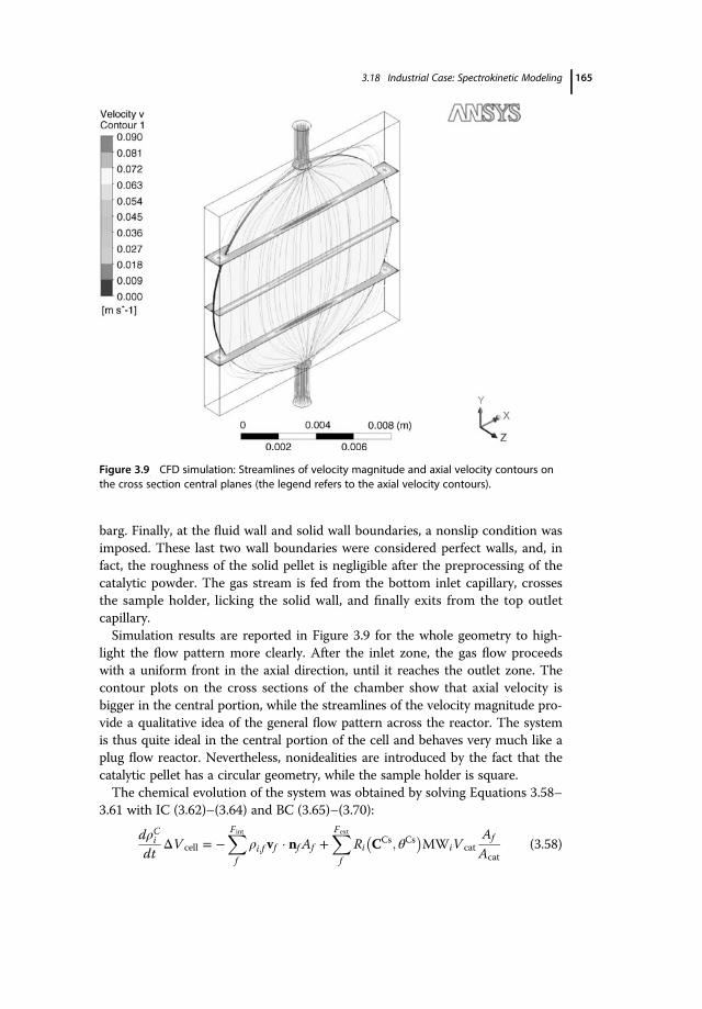
barg. Finally, at the fluid wall and solid wall boundaries, a nonslip condition wasimposed. These last two wall boundaries were considered perfect walls, and, infact, the roughness of the solid pellet is negligible after the preprocessing of thecatalytic powder. The gas stream is fed from the bottom inlet capillary, crossesthe sample holder, licking the solid wall, and finally exits from the top outletcapillary.Simulation results are reported in Figure 3.9 for the whole geometry to high-

light the flow pattern more clearly. After the inlet zone, the gas flow proceedswith a uniform front in the axial direction, until it reaches the outlet zone. Thecontour plots on the cross sections of the chamber show that axial velocity isbigger in the central portion, while the streamlines of the velocity magnitude pro-vide a qualitative idea of the general flow pattern across the reactor. The systemis thus quite ideal in the central portion of the cell and behaves very much like aplug flow reactor. Nevertheless, nonidealities are introduced by the fact that thecatalytic pellet has a circular geometry, while the sample holder is square.The chemical evolution of the system was obtained by solving Equations 3.58–

3.61 with IC (3.62)–(3.64) and BC (3.65)–(3.70):

dρCidt

ΔV cell � �XF int

f

ρi;f vf � nf Af �XFext

f

Ri CCs; θCs� �

MWiV catAf

Acat(3.58)

Figure 3.9 CFD simulation: Streamlines of velocity magnitude and axial velocity contours onthe cross section central planes (the legend refers to the axial velocity contours).


Ωsite

dθCsjdt

� σjRj CCs; θCs

� �(3.59)

θCsPt � 1 � θCsPt�O (3.60)

θCsBaO � 1 � θCsNitrite � θCsNitrate (3.61)

IC:

ρCi�O2�t � 0; c ∈ gas� � 0:03 � P �MWO2

RT(3.62)

ρCi ≠ O2�t � 0; c ∈ gas� � 0 (3.63)

θCsj �t � 0� � 0 (3.64)

BC:

ρCO2�t � 0; c ∈ @ inlet� � 0:03 � P �MWO2

RT(3.65)

ρCNO�t � 0; c ∈ @ inlet� � 1000 �ppm� � P �MWNO

RT(3.66)

ρCNO2�t � 0; c ∈ @ inlet� � 0 (3.67)

rρCi �t > 0; c ∈ @ outlet� � 0 (3.68)

�nf �Nci �t > 0; c ∈ @ fluid wall� � 0 (3.69)

�nf �Nci �t > 0; c ∈ @ solid wall� � RiMWiVCAT

Af

ACAT(3.70)

In Equations 3.58–3.70, subscript i refers to gas-phase reactants and products(O2, NO, NO2), subscript j refers to adspecies (Pt–O, NO2

�, NO3�), while super-

script c refers to gas-phase cell threads.The resulting ODE system is made up of ∼50 000 equations, and is character-

ized by a diagonally dominant, sparse Jacobian matrix (Figure 3.10). We shouldhighlight the presence of three bigger diagonal blocks, which refer to the accu-mulation and convective terms of the three gas-phase species (NO, NO2, O2),and three smaller diagonal blocks, which refer to the adspecies (NO2

�,NO3�,

and PtO). The nondiagonal blocks are related to the reaction term.

3.18.7

CAT-PP Simulation Results

The time evolution of the concentrations of NO and NO2 and of the surfacecoverage of nitrites and nitrates upon stepwise exposure of the catalyst sampleto a NO–O2 mixture at 250 °C is shown in Figure 3.11 as a representative exam-ple of the simulation results. At this temperature, NO storage proceeds via a“front mechanism,” which results in complete NOx uptake for the first tens ofseconds, followed by a progressive breakthrough of NO, which reaches an outlet


concentration equal to the inlet concentration in around 500 s. In the first 300 s,NO is stored mainly in the form of nitrites, which are then converted to nitratesstarting from the fraction of the catalyst pellet closer to the cell inlet. In fact,after about 400 s, the nitrites reach their maximum concentration, while givenlonger exposure times, they are oxidized to nitrates (reaction S5). The latter

Figure 3.10 Jacobian matrix structure.

Figure 3.11 Gas-phase composition fields and space-time evolution of surface coverage @ T= 250 °C.


species, however, displays a monotonic increase with time, at a rate thatincreases with time as is typical of secondary reaction products. Interestingly,simulation results demonstrate that at 250 °C the nitrite route is faster than thenitrate route at the start of NOx uptake and leads to the formation of nitrites asprecursors to the formation of nitrates: The surface concentration of nitrites is,in fact, greater than that of nitrates for the first 900 s.The results of the simulation allow us to evaluate the extent of the non-

idealities of the simulated operando FTIR reaction cell. A comparison of thesimulation results obtained with the CAT-PP and with the ideal PFR modelis provided in Figure 3.12, in which the experimental data, the results of thesimulation with the ideal reactor mode, and the results of CAT-PP are com-pared (Corbetta et al., 2014). It is clear that the ideal PFR and the CAT-PPsimulations are in good agreement with each other. This proves that theadopted FTIR cell may be described as an ideal reactor or not, thus provingan ex-postvalidation of the hypothesis done by Visconti et al. (2013) todevelop a spectrokinetic model for the NOx storage over a representativeLNT catalyst on the basis of a set of transient surface and gas-phase exper-imental data collected in such a cell.Nevertheless, CAT-PP is a move in the direction of finding a better fit for the

experimental data. Such encouraging results demonstrate that CFD simulationof reactive systems can be performed with an acceptable computational effort.Thus, a numerical methodology was developed to simulate diluted hetero-

geneous reactive systems based on a CFD approach. This approach consistsof two main steps. Initially, a nonreactive CFD simulation is performed usingcommercial code, and, in the second step, hydrodynamic data are transferredto a postprocessor capable of solving the transport equations of the chemicalspecies.

0

0.1

0.2

0.3

0.4

0.5

0.6

0.7

0.8

0.91

10009008007006005004003002001000

Su

rfac

e co

vera

ge

[-]

Time [s]

NO2- CFD NO3- CFD NO2- PFR NO3- PFR NO2- exp NO3- exp

Figure 3.12 Surface-averaged coverage of the adspecies on the IR beam invested area@ 250 °C.


The methodology is highly adaptable and can handle arbitrary geometries anddetailed kinetic schemes. Moreover, the simplification assumptions allow thesereactive systems to be properly modeled without the compulsory need for a clus-ter workstation facility.Its application to the case of the LNT lean-phase accumulation demonstrated

its numerical viability and prediction superiority over other existing methods.Comparisons between CAT-PP and ideal PFR models highlight the substantialideality of the system analyzed, while the first approach might provide furtherinformation on the dynamic and spatial behavior of active surface coverage dur-ing the catalyst operation.The simulator will also be able to investigate different geometries, making pos-

sible a sensitivity analysis of cell performance in relation to geometrical lengthsand the position and dimension of the irradiated zone.

3.18.8

Nomenclature

Symbol Dimension Description

T s TimeT K Reaction temperatureR J/(mol K) Ideal gas constantXi — Molar fraction of the ith gaseous speciesθj — Surface coverage of the jth adspeciesϱCi kg/m3 Massive concentration of ith gaseous species on cell C centroidϱfi kg/m3 Massive concentration of ith gaseous species on face f centroidΔVcell m3 Computational cell volumeVf m/s Mesh face velocityAf m2 Face areaNf — Face normal vectorNfaces — Number of faces of a computational cellFint — Number of internal faces of a computational cellFext — Number of boundary faces (on solid wall) of a computational cellni kg/s Mass fluxRi mol/(m3 s) Reaction source termMWi g/mol Molar weightVcat m3 Catalyst overall volumeAcat m2 Catalyst geometrical external areaΩsite mol/m3 Active site concentration (load)σj — Coordination number of jth adspecies


4Differential and Algebraic Equation Systems

Examples from this chapter can be found in Vol4_Chapter4 directory in theWileyVol4.zip file available at the following web site:http://www.chem.polimi.it/homes/gbuzzi.

4.1Introduction

This chapter deals with the numerical solution of initial value problems in differ-ential– algebraic equations.

A differential– algebraic equations system is indicated with the acronym DAE.

It is worth stressing that a DAE problem is very different from an ODE problem,especially in its general formulation (Ascher and Petzold, 1998).

In a DAE problem, two new concepts are fundamental: the index of the systemand its solvability (Ascher and Petzold, 1998). To understand the index concept,consider the general DAE problem:

f y; y´; t� � � 0 (4.1)

The following systems of equations are obtained by progressively differentiat-ing the system (4.1):

df y; y´; t� �dt

� 0 (4.2)

. . .

d�j�f y; y´; t� �dt�j� � 0 (4.3)

This system can be written as follows:

f 0� � y; y´; t� � � 0 (4.4)

171



f 1� � y; y´; y´´; t� � � 0 (4.5)

. . .

f j� � y; y´; . . . ; y j�1� �; t� � � 0 (4.6)

The minimum number of times that we need to differentiate the original systemto obtain a system f j� � y; y´; . . . ; y j�1� �; t

� � � 0 that uniquely determines the vectory´ as a continuous function of y and t is the index of the DAE.

An ODE system is a DAE system with index 0.Let us consider the special case of a semiexplicit DAE:

y´ � f y; x; t� � (4.7)

0 � g y; x; t� � (4.8)

If we differentiate the algebraic Equation 4.8 with respect to t, we obtain

y´ � f y; x; t� � (4.9)

gx y; x; t� �x´ � gy y; x; t� �y´ � �gt y; x; t� � (4.10)

If gx is nonsingular, the systems (4.9) and (4.10) are an implicit ODE and wecan say that the original problem has index 1.

The semiexplicit DAE (4.9) and (4.10) are index 1 if, and only if, gx isnonsingular.

Below, only the special case of semiexplicit DAE with nonsingular gx, which is ofgreat interest in practical cases, is considered.

For the sake of clarity, the features of the selected problem are reported:

1) It must consists of ny explicit differential equations with respect to ny firstderivatives of y:

y´ � f y; x; t� � (4.11)

and nx algebraic equations:

0 � g y; x; t� � (4.12)

where nx is the number of variables x.2) The system (4.12) must be solvable with respect to the variables x with

assigned values of the variables y.

In particular, the system (4.12) must be solvable in a stable way once the initialvalues of the vector y are assigned.

If the two previous conditions are verified, the semiexplicit DAE (4.11) and(4.12) are solvable.

172 4 Differential and Algebraic Equation Systems

The concept of solvability of a DAE is much more complex in problems otherthan the one considered in (4.11) and (4.12). It is complex also in the case oflinear equations when they are not in the semiexplicit form and it is very com-plex in the general case. We refer readers to the literature (Ascher and Petzold,1998) for an in-depth description.

As remarked many times in this series of volumes, it is crucial to

1) know the physical problem that we are solving,2) formulate the problem so as not to introduce any ill-conditioning, and3) use a program that does not introduce any instability into the problem

solution.

Consider the problem of characterizing the movement of a simple oscillator: Asmall mass m placed at the extreme of a stiff rod of length L oscillates underideal conditions (friction neither in the mechanical components nor in themovement itself) due to the gravity. If we indicate with F the tension on the rodand with mg the force of gravity, the equations modeling the motion, in Carte-sian coordinates, are given by

mx´´ � � FxL

my´´ � � FyL

�mg

x2 � y2 � L2 � 0

Thus, it is a DAE system that requires four initial conditions: x 0� � � x0;x´ 0� � � x0; y 0� � � y0; y

´ 0� � � y0.Conversely, because we are aware of the physical problem, it is clear that only

two conditions are truly independent: the angle of the rod with respect to theordinate axis, φ, and the angle velocity at the initial conditions.If the same problem is described using φ as independent variable, the problem is

φ´´ � � gLsin φ� �

This is a simple differential equation that requires only two initial conditionsas required by the physical problem. From a mathematical point of view, it ispossible to switch from the first to the second formulation using x � L sin φ� �and y � �L cos φ� �, but the first formulation will not be entertained by anyonefamiliar with the physical problem for several reasons.Since Galileo, we have known that the oscillator does not depend on the mass

(if we assume that no friction is present). In the formulation of Cartesian coor-dinates, it seems that mass m plays some kind of role in oscillator movement.Moreover, if the rod is stiff, its length is constant and it is not necessary to insertan equation to verify it. Last but not least, another important consideration forother problems is that the equations have to be written, when possible, with

4.1 Introduction 173

degrees of freedom strictly connected to the physical problem and, therefore,with the correct number of degrees of freedom: 2 in this case and not 4.

Also in the special case of semiexplicit DAE, a particular problem could beinsolvable within a certain range of t due to the algebraic portion.

In Section 3.12, the Van der Pol oscillator system is integrated:

y1 � y2

y2 � 1 � y21� �

y2 � y1ε

with ε a small nonzero number. This system can be integrated starting fromy1 0� � � 2, y2 0� � � 0 between t � 0 and tout � 1; 2; 3; 4; 5; 6; 7; 8; 9; 10; 11.If we assign ε � 0, we obtain a DAE system:

y1 � y21 � y21� �

y2 � y1 � 0

In this kind of case, it is no longer possible to integrate the system between t �0 and tout � 1 by starting from y1 0� � � 2, y2 0� � � y1 0� �= 1 � y21 0� ��

since whent tends to 1, y1 also tends to 1 and it makes the algebraic system singular.

4.2Multivalue Method

The idea of using a multivalue method to solve DAE problems was introducedby Gear (1971). As demonstrated in Chapter 2, given a system in the followingimplicit form:

f y m� �; y m�1� �; . . . ; y´; y; t� � � 0 (4.13)

it is sufficient to replace each derivative with the corresponding component ofthe Nordsieck vector to have a nonlinear system in the single unknown b. Someequations of the system may be algebraic equations.Although DAE problems of any index should be solved theoretically, serious

numerical problems may arise in a general program. As seen in Chapter 2, inthe case of ODEs too, the explicit form has special features that can be exploitedto solve, in a stable manner, the corresponding nonlinear system:

v1 � b � hf v0 � r0b; tn�1� � � 0 (4.14)

Even the special case of semiexplicit DAE with nonsingular gx has peculiarfeatures that make the system rather easy to solve. The nonlinear system in thiscase becomes

v1 � b � hf v0 � r0b;w0 � r0b; tn�1� � � 0 (4.15)

g v0 � r0b;w0 � r0b; tn�1� � � 0 (4.16)


In this special problem, it was possible to remove the integration step h from thealgebraic system since algebraic equations must be equal to 0. It makes the Jaco-bian of the system significantly better conditioned.

One significant difference, probably the most significant of all, between anODE where the system (4.14) has to be solved and a DAE where the systems(4.15) and (4.16) have to be solved lies in the fact that in an ODE system theJacobian tends to the identity matrix when the integration step h decreases,whereas this is no longer the case for DAE systems. In this latter instance, wegenerally encounter much greater difficulty in adequately solving the corre-sponding nonlinear system.

When the algebraic portion is strongly nonlinear, the devices described in Sec-tion 2.16 for ODE problems may not be sufficient.

In these cases, it is useful to adopt a more robust program for the solution ofthe nonlinear system (see Vol. 3, Buzzi-Ferraris and Manenti, 2014).

4.3DAE Classes in the BzzMath Library

The following classes, which are based on multivalue algorithms, are imple-mented in the BzzMath library.

BzzDaeBzzDaeSparseBzzDaeObjectBzzDaeSparseObject

The BzzDae class has two constructors:

BzzDae dae1(y0,t0,ider,DaeSample);BzzDae dae2;dae2(y0,t0,ider,DaeSample);

The first constructor has the following in its argument:

� The BzzVector y0, which contains the initial values of y.� The double t0, initial value of the independent variable, t0.� The BzzVectorInt ider, which contains the Boolean information requiredto distinguish between differential and algebraic equations: if the ith compo-nent is 1, the corresponding equation is differential; it is algebraic when theith component is null.� The name of the function where the system is calculated, DaeSample.

The second constructor is the default constructor. Once defined as an objectof the BzzDae class, it can be initialized using the overlapped operator () withthe same argument as the previous constructor.

4.3 DAE Classes in the BzzMath Library 175

Using the operator (), it is possible to reinitialize an object with a new start-ing point and/or with the name of the same function or of a different function aswell where a novel system to be integrated is implemented.The user must provide the prototype declaration for the function f y; t� �, where

the system is calculated before defining an object that uses it within the pro-gram. The function input is the vector y and the corresponding t, which aremanaged by the object. The output is the vector f . For efficiency purposes aswell as for ease of use, the vectors y and f are both BzzVector references.


Example 4.1

Integrate the following system:

r1 � 0:04y1r2 � 104y2y3r3 � 3 ? 1014y22

y1 � �r1 � r2

y2 � r1 � r2 � r3

y1 � y2 � y3 � 1 � 0

in the range t � 0; 100� �.Note that

BzzVectorInt iDer(3,1,1,0)

since the first two variables are differential, whereas the third one is algebraic.The program is

#define BZZ_COMPILER 0#include “BzzMath.hpp”//prototypevoid BzzDaeRobertson(BzzVector &y,double t,


{BzzVector y0(3,1.,0.,0.),y;double t0 = 0.,tOut = 100.;BzzVectorInt iDer(3,1,1,0);BzzDae dae(y0,t0,iDer,BzzDaeRobertson);BzzVector yMin(3);dae.SetMinimumConstraints(&yMin);y = dae(tOut);dae.BzzPrint(“Results”);}


void BzzDaeRobertson(BzzVector &y,double t,BzzVector &f)

{double r1 = .04 * y[1];double r2 = 1.e4 * y[2] * y[3];double r3 = 3.e14 * y[2] * y[2];f[1] = -r1 + r2;f[2] = r1 - r2 - r3;f[3] = y[1] + y[2] + y[3] - 1.;}

The BzzDaeObject class is different from the previous BzzDae class becauseits objects are initialized with an object rather than the name of the function.

BzzOdeDaeObjetct dae1(y0,t0,ider, &DaeSampleObject);BzzOdeNonStiff dae2;dae2(y0,t0,ider, &DaeSampleObject);

The object DaeSampleObject must belong to a class created by the user andderived from the class BzzDaeSystemObject. The user must provide twofunctions:

GetSystemFunctionsObjectBzzPrint

The first is required to define the system, the second to customize the printoutof the results. The class must contain a constructor to initialize the data used inthe aforementioned functions. The use of global variables is avoided.

Example 4.2

Integrate the same problem as in the previous example using an object of theclass BzzDaeObject. The program is

#define BZZ_COMPILER 0#include “BzzMath.hpp”class MyDaeSystemObject : public BzzDaeSystemObject

{private:

BzzVector data;public:

MyDaeSystemObject(BzzVector &dat){data = dat;}

virtual void GetSystemFunctions(BzzVector &y,double t,BzzVector &f);

virtual void ObjectBzzPrint(void);};


void MyDaeSystemObject::ObjectBzzPrint(void){::BzzPrint(“\n\nObject Print”);data.BzzPrint(“Data”);}

void MyDaeSystemObject::GetSystemFunctions(BzzVector &y,double t,BzzVector &f)

{double r1 = data[1] * y[1];double r2 = data[2] * y[2] * y[3];double r3 = data[3] * y[2] * y[2];f[1] = -r1 + r2;f[2] = r1 - r2 - r3;f[3] = y[1] + y[2] + y[3] - 1.;}

void main(void){BzzVector y0(3,1.,0.,0.),y;double t0 = 0.,tOut = 100.;BzzVectorInt iDer(3,1,1,0);BzzVector data(3,0.04,1.e4,1.e14);MyDaeSystemObject objDae(data);BzzDaeObject dae(y0,t0,iDer, &objDae);BzzVector yMin(3);dae.SetMinimumConstraints(&yMin);y = dae(tOut);dae.BzzPrint(“Results”);}

An object from all the previous classes, as it is defined, automatically receives adefault value for the tolerances of the absolute (1.e-10) and relative (1.e-6)

errors on the variables yi.It is possible to modify the default values of such tolerances using the func-

tions SetTolAbs and SetTolRel, which accept as their argument both a singlevalue for all the variables or a BzzVector to assign a special tolerance to eachvariable:

BzzVector tolAbs(3,1.e-3,1.e-4,1.e-5);BzzVector tolRel(3,.001,.0001,.00001);double tolA = 1.e-5; // default 1.e-10double tolR = 1.e-4; // default 1.e-6o1.SetTolAbs(tolAbs);o2.SetTolRel(tolRel);o3.SetTolAbs(tolA);o4.SetTolRel(tolR);


The objects from these classes not only remember their history but also exploitthe multivalue method property of keeping the optimal integration step dis-joined from user requests.

If the user uses the object for progressively increased tOut, the integration isnot performed by starting from t0 each time, but from the value of t achievedin the previous iteration with an already estimated integration step. Moreover,the integration step generally adopted in practice overcomes the value of tOut

for which the vector y is required. If we want to prevent this integration stepgoing beyond an assigned value, we only have to add that value as an argumentof the operator (). For example:

y = dae(tOut,tCritic);

Objects in these classes can use certain special functions:

� SetMinimumConstraints� SetMaximumConstraints

These functions provide bounds to the integration variables y. If one of themachieves the bound, the object automatically considers this relation to be analgebraic equation by preventing any violation.Example:

BzzVector yMin(numVariables);BzzVector yMax(numVariables);yMax = 1.;dae.SetMinimumConstraints(yMin);dae.SetMaximumConstraints(yMax);

� StepPrint

There are three versions of this function. They allow a print to be carried outonto a selected file of the values of the variables t and y in correspondence withthe mesh points used during the integration.The first function requires only the name of the file. All the values of the vari-

ables y are printed out.Example:

o.StepPrint(“RESULTS.TXT”);

The second version requires as its argument both the name of the file and aBzzVectorInt where the indices of the variables to be printed are provided. Itis also possible to add a comment. Example:

BzzVectorInt lv(2);lv[1] = 1; lv[2] = 3;dae.StepPrint(“RESULTS2.TXT”,lv,“Variables 1 and 3”);


The third version requires as its argument the name of a function provided bythe user indicating what is to be printed. Example:

dae.StepPrint(MyPrint);

This function is automatically invoked at each integration step and with theappropriate value of t and its corresponding y and must also have the followingargument:

void MyPrint(BzzVector &y,double t);

� StepDebug

There are several version of this function. The simplest one requires justthe name of the file used for printing the relevant information such as thevalue of t, the integration step, the variable with maximum error, and thevalue of the error.Example:

dae.StepDebug(“debug.txt”);

� GetInitAndEndTimeStep

This function allows us to find the values at the beginning and at the end ofeach integration step effectively used. Example:

dae.GetInitAndEndTimeStep(&tInitStep, &tEndStep);

� GetTimeInMeshPoint� GetYInMeshPoint� GetY1InMeshPoint

These functions allow us to find t, y, and y´ for each integration step.

Additional examples and tests of the use ofBzzDae, andBzzDaeObject classes can be found inBzzMath/Examples/BzzMathAdvanced/Dae

directory and

DaeDaeObject


Objects from the BzzDaeSparse and BzzDaeSparseObject classes exploitthe devices broached in Section 2.16.2.4 when the Jacobian matrix is sparse.



These classes use different constructors to indicate the kind of Jacobian struc-ture. The simplest cases are as follows:

� Sparse and unstructured Jacobian.In this case, the user must provide the indices of the rows and columns where

the Jacobian is nonzero. This can be done in two ways: using two BzzVector-

Int containing the index row and column of each nonzero element or using anobject from the BzzMatrixCoefficientsExistence class.In the former case, we have

BzzDaeSparse o;BzzVectorInt r(numElements,1,1,2,2,3, . . . );BzzVectorInt c(numElements,1,4,3,7,8...);o(y0,t0,indexOdeAlg,DaeSparseGeneric, &r, &c);

In the latter case, we have

BzzMatrixCoefficientsExistence Je(300,300);Je(1,1),Je(1,4),Je(2,3),Je(2,7),Je(3,8), . . . ...;BzzDaeSparse o(y0,t0,ider,DaeSparseGeneric, &Je);

� Band JacobianIn this case, we need to indicate only the upper and lower band values.

BzzDaeSparse dae(y0,t0,ider,DaeBand,5,7);

� Tridiagonal blocks JacobianIn this case, we need to indicate only the size of the blocks on the three

diagonals.

BzzDaeSparse dae(y0,t0,ider,DaeTridiagonalBlock,4);

Example 4.3


xx x

xxxxxx x

xx xxxxx x

It is a sparse matrix that will be treated in this example as though it does nothave any particular structure. Suppose that the equations 2, 4, 6, 8 are algebraicand the remaining ones are differential. The program is

#define BZZ_COMPILER 0 // Visual C++ 6 Compiler


#include “BzzMath.hpp”void DaeSparseGeneric (BzzVector &y,


{int N = 8;BzzVector y0(N);y0(1) = 5.; y0(2) = 0.1; y0(3) = -3.1;y0(4) = -1.1; y0(5) = 10.; y0(6) = 38.;y0(7) = 11.; y0(8) = 8.;BzzVectorInt indexOdeAlg(8);indexOdeAlg(1) = 1; indexOdeAlg(2) = 0;indexOdeAlg(3) = 1; indexOdeAlg(4) = 0;indexOdeAlg(5) = 1; indexOdeAlg(6) = 0;indexOdeAlg(7) = 1; indexOdeAlg(8) = 0;double t0 = 0.,tOut = 1.;BzzVector y;BzzDaeSparse o;BzzVectorInt r(18,1,2,2,3,3,3,4,4,5,5,6,6,6,

7,7,7,8,8);BzzVectorInt c(18,1,2,4,1,2,3,3,4,3,5,5,6,8,

5,6,7,5,8);o(y0,t0,indexOdeAlg,DaeSparseGeneric, &r, &c);

// BzzMatrixCoefficientsExistence Je(8,8);// Je(1,1),// Je(2,2),Je(2,4),// Je(3,1),Je(3,2),Je(3,3),// Je(4,3),Je(4,4),// Je(5,3),Je(5,5),// Je(6,5),Je(6,6),Je(6,8),// Je(7,5),Je(7,6),Je(7,7),// Je(8,5),Je(8,8);// o(y0,t0,indexOdeAlg,DaeSparseGeneric, &Je);

y = o(tOut);o.BzzPrint(“Results”);}

void DaeSparseGeneric(BzzVector &y,double t,BzzVector &dy){dy(1) = -y(1);dy(2) = y(2) + y(4) + 1.;dy(3) = y(3) - y(2) - y(1);dy(4) = y(4) - y(3) - 2.;dy(5) = -y(3) + y(5);dy(6) = y(5) - y(6) + 3. *y(8) + 4.;dy(7) = y(5) - y(6) - y(7);dy(8) = y(5) - y(8) - 2.;}


Note that the object was initialized as follows:

o(y0,t0,indexOdeAlg,DaeSparseGeneric, &r, &c);

An alternative way of achieving the same thing is to use an object from theBzzMatrixCoefficientsExistence class:

o(y0,t0,indexOdeAlg,DaeSparseGeneric, &Je);

This alternative was adopted in release 6 of the BzzMath library and is consid-ered obsolete since a more efficient solver for linear systems is adopted in theother initialization.

Example 4.4

The same problem as seen in the previous example is solved as it has a bandstructure with a lower bandwidth equal to 3 and upper bandwidth equal to 2.The program is

#define BZZ_COMPILER 0 // Visual C++ 6 Compiler#include “BzzMath.hpp”Void DaeBand(BzzVector &y,double t,BzzVector &f);void main(void)

{int N = 8;BzzVector y0(N);y0(1) = 5.; y0(2) = 0.1; y0(3) = -3.1;y0(4) = -1.1; y0(5) = 10.; y0(6) = 38.;y0(7) = 11.; y0(8) = 8.;BzzVectorInt indexOdeAlg(8);indexOdeAlg(1) = 1; indexOdeAlg(2) = 0;indexOdeAlg(3) = 1; indexOdeAlg(4) = 0;indexOdeAlg(5) = 1; indexOdeAlg(6) = 0;indexOdeAlg(7) = 1; indexOdeAlg(8) = 0;double t0 = 0.,tOut = 1.;BzzVector y;BzzDaeSparse o;o(y0,t0,indexOdeAlg,DaeBand,3,2);y = o(tOut);o.BzzPrint(“Results”);}

void DaeBand(BzzVector &y,double t,BzzVector &dy){dy(1) = -y(1);dy(2) = y(2) + y(4) + 1.;dy(3) = y(3) - y(2) - y(1);dy(4) = y(4) - y(3) - 2.;dy(5) = -y(3) + y(5);


dy(6) = y(5) - y(6) + 3. *y(8) + 4.;dy(7) = y(5) - y(6) - y(7);dy(8) = y(5) - y(8) - 2.;}

Note that the object was initialized as follows and we only need to point outthat the system has lower and upper bandwidths 3 and 2, respectively:

o(y0,t0,indexOdeAlg,DaeBand,3,2);

Example 4.5

The previous problem is solved in this example as it has a tridiagonal blockstructure with block sizes 2× 2. The program is

#define BZZ_COMPILER 0 // Visual C++ 6 Compiler#include “BzzMath.hpp”void DaeTridiagonalBlock(BzzVector &y,


{int N = 8;BzzVector y0(N);y0(1) = 5.; y0(2) = 0.1; y0(3) = -3.1;y0(4) = -1.1; y0(5) = 10.; y0(6) = 38.;y0(7) = 11.; y0(8) = 8.;BzzVectorInt indexOdeAlg(8);indexOdeAlg(1) = 1; indexOdeAlg(2) = 0;indexOdeAlg(3) = 1; indexOdeAlg(4) = 0;indexOdeAlg(5) = 1; indexOdeAlg(6) = 0;indexOdeAlg(7) = 1; indexOdeAlg(8) = 0;double t0 = 0.,tOut = 1.;BzzVector y;BzzDaeSparse o;o(y0,t0,indexOdeAlg,DaeTridiagonalBlock,2);y = o(tOut);o.BzzPrint(“Results”);}

void DaeTridiagonalBlock(BzzVector &y,double t,BzzVector &dy)

{dy(1) = -y(1);dy(2) = y(2) + y(4) + 1.;dy(3) = y(3) - y(2) - y(1);dy(4) = y(4) - y(3) - 2.;dy(5) = -y(3) + y(5);dy(6) = y(5) - y(6) + 3. * y(8) + 4.;


dy(7) = y(5) - y(6) - y(7);dy(8) = y(5) - y(8) - 2.;}

Note that the object was initialized as follows and we only need to point outthat the system is tridiagonal blocks with 2× 2 block sizes:

o(y0,t0,indexOdeAlg,DaeTridiagonalBlock,2);

An example using tridiagonal blocks structure is provided in Section 5.5.

Jacobian structures other than the ones analyzed here will be broached inChapter 5.

Additional examples and tests of the use ofBzzDaeSparse, andBzzDaeSparseObject classes can be found inBzzMath/Examples/BzzMathAdvanced/Dae

directory and

DaeSparseDaeSparseObjectDaeSparseObjectTests




5DAE: Case Studies


5.1Introduction

This chapter presents a collection of case studies involving DAE systems. Thecase studies come from theoretical tests that are well established in the litera-ture, from real problems and those usually characterized by a larger number ofvariables.

5.2Van der Pol Oscillator

One of the simplest nonlinear equation systems describing a circuit is Van derPol’s system (Hairer and Wanner, 2010):

y1 � y2

y2 � 1 � y21� �

y2 � y1ε

with y1 0� � � 2 and y2 0� � � 0.This problem consists of two ODE equations and when ε is very small, the

problem is stiff. If ε � 0; the problem is the DAE system:

y1 � y2

1 � y21� �

y2 � y1 � 0

187



Example 5.1

Integrate the Van der Pol DAE system with the initial condition y1 0� � � 2,while y2 0� � must satisfy the algebraic equation. It is not possible to integratethis system between t � 0 and tout � 1 because when y1 decreases andachieves the value 1, the algebraic equation becomes singular and y2 tends toinfinite.The integration will be carried out between t � 0 and tOut � 8:068e-001. The

program is

#define BZZ_COMPILER 0 // Visual C++ 6 Compiler#include “BzzMath.hpp”void VanDerPolDae(BzzVector &y,double t,


{BzzPrint(“\n\nVan Der Pol Dae Problem”);BzzVector y0(2,2.,0.),y;BzzVectorInt iDer(2,1,0);double t0 = 0.,tOut = 8.068e-001;BzzDae o(y0,t0,iDer,VanDerPolDae);o.StepPrint(“VanDerPolDae.txt”);y = o(tOut,tOut);o.BzzPrint(“Results”);}

void VanDerPolDae(BzzVector &y,double t,BzzVector &f){f[1] = y[2];f[2] = (1. - BzzPow2(y[1])) * y[2] - y[1];}

Note that we inserted the statement

y = o(tOut,tOut);

to prevent the new mesh point from being located beyond the tOut. Because thestatement

o.StepPrint(“VanDerPolDae.txt”);

has been inserted, the result of every step is printed on the file VanDerPolDae.

txt. Moreover, using the statement

o.BzzPrint(“Results”);

the result of the integration is printed onto BzzFile.txt. It results in

y1 1.00388647649379e+000y2 -1.28900749935993e+002

188 5 DAE: Case Studies

5.3Regression Problems with the DAE Model

Chemical engineers sometimes encounter problems in evaluating certain ofthe parameters required to adapt their mathematical models to real chemicalplant behavior or to certain experimental/industrial data collected in thefield. One typical case is the estimation of kinetic parameters (preexponentialfactor and activation energy) for detailed or lumped reaction systems such ascombustion processes, gasification, synthesis of base chemicals, and com-modities. The mathematical problem consists of an optimization, which isoften reduced to a least sum of square, subject to differential models thatrepresent the real system reasonably well. Thus, the overall problem involvesnonlinear programming with the constraints consisting of differential–alge-braic equations (DAEs) and with physical bounds on the variables anddegrees of freedom.

In the BzzMath library, the BzzNolLinearRegression class is developed toestimate the parameters of a nonlinear model.

An object from the BzzNolLinearRegression class includes numerousconstructors and functions that allow us to select the most appropriate criterionto estimate the model parameters. In the following example, the target is to min-imize the deviation between the mathematical model and the experimental data.The function where the dependent variables are calculated must have the follow-ing argument:

(int model,int ex,BzzVector &b,BzzVector &x,BzzVector &y)

where

� model is the index of the model for which we want to estimate theparameters (to be used when several models have to be analyzedsimultaneously);� ex is the index of the experiment, which varies from 1 to numExperi-

ments. It is helpful to prevent useless calculations as reported in the follow-ing example;� b is the value of the parameters that must be estimated;� x is the value of the independent variables in correspondence with the indexex;� y is the value of the dependent variables calculated in correspondence withthe index ex.

The user must not modify the values of b and x inside this function.

5.3 Regression Problems with the DAE Model 189

Example 5.2

Consider the theoretical model (see Buzzi-Ferraris and Manenti, 2010b)

dy1dt

� �β1y1 � β2y2y3

dy2dt

� β1y1 � β2y2y3 � β3y22

y1 � y2 � y3 � 1 � 0

(5.1)

consisting of a system of differential–algebraic equations. Experimental dataconsist of the values of the three dependent variables at different values of t andthey are available in the following program. The regression problem consists ofthe optimal estimation of the model parameters β once the data of the vectors yfor different values of the variable t have been assigned.Theoretically, the first parameter is on the order of 1:, the second is some

tens larger than the first, and the third parameter is significantly largerthan the others. 1:; 10:; 100:f g is assumed as the initial guess; the optimalvalues are

1 4.13090298962625e-0012 1.12352704754714e+0033 1.53619407391221e+005

As can be seen in the following program, two functions are needed. First,

void ModelDaeExample(int model,int ex,BzzVector &b,BzzVector &x,BzzVector &y);

is required to evaluate the function minimum for evaluating the model parame-ters. Second,

void BzzDaeExample(BzzVector &y,double t,BzzVector &f);

is required to integrate the differential–algebraic system.

As in Section 3.13, it is possible to optimize the code by means of the variableex.

As the values of the dependent variables can be obtained through a single inte-gration of the system, in the function ModelDaeExample, they are all evaluatedin correspondence with the first experimental point, where ex is equal to 1. Allthe dependent variables are collected in the auxiliary BzzMatrix Y and they arethen recovered in correspondence with the value ex of the experimental point.By adopting this device, we do not have to repeat the integration to achieve allthe experimental points. The auxiliary matrix and other variables used at each


iteration of the model are declared static in order to prevent them from beingcontinuously resized.To inform the program about the nature (differential or algebraic) of the equa-

tions, the object BzzVectorInt iDer(3,1,1,0) is introduced in the con-structor of the object BzzDae dae. A value equal to 1 denotes a differentialequation, whereas a null value denotes an algebraic equation.The program is

#include “BzzMath.hpp”void ModelDaeExample(int model,int ex,

BzzVector &b,BzzVector &x,BzzVector &y);void BzzDaeExample(BzzVector &y,double t,

BzzVector &f);int numDaeExperiments;BzzVector bDaeExample,tDaeExample;void main(void)

{BzzPrint(“\n\nModelDaeExample”);BzzPrint(“\n\nnumModels 1 numX 1 numY 3”);int numModels = 1;int numX = 1;int numY = 3;int numExperiments = 29;numDaeExperiments = numExperiments;BzzMatrix X(numExperiments,numX,

.1,.2,.3,.4,.5,.6,.7,.8,.9,1.,2.,3.,4.,5.,6.,7.,8.,9.,10.,100.,200.,300.,400.,500.,600.,700.,800.,900.,1000.);

int i;ChangeDimensions(numExperiments, &tDaeExample);for(i = 1;i <= numExperiments;i++)

tDaeExample[i] = X[i][1];BzzMatrix Y(numExperiments,numY,

9.636e-001,1.488e-003,3.689e-002,9.338e-001,1.358e-003,6.984e-002,9.047e-001,1.254e-003,9.107e-002,8.861e-001,1.177e-003,1.148e-001,8.582e-001,1.109e-003,1.377e-001,8.464e-001,1.045e-003,1.525e-001,8.274e-001,1.001e-003,1.706e-001,8.189e-001,9.493e-004,1.832e-001,8.035e-001,9.122e-004,1.996e-001,7.872e-001,8.815e-004,2.089e-001,7.040e-001,6.638e-004,2.994e-001,6.442e-001,5.551e-004,3.563e-001,6.005e-001,4.802e-004,3.941e-001,5.735e-001,4.320e-004,4.301e-001,

5.3 Regression Problems with the DAE Model 191

5.482e-001,3.979e-004,4.484e-001,5.210e-001,3.656e-004,4.766e-001,5.077e-001,3.437e-004,4.929e-001,4.838e-001,3.217e-004,5.159e-001,4.707e-001,3.076e-004,5.290e-001,1.833e-001,7.939e-005,8.166e-001,1.213e-001,5.093e-005,8.826e-001,9.502e-002,3.907e-005,9.069e-001,7.311e-002,2.874e-005,9.209e-001,6.273e-002,2.795e-005,9.372e-001,5.749e-002,1.654e-005,9.465e-001,4.821e-002,1.999e-005,9.478e-001,4.526e-002,1.499e-005,9.587e-001,3.925e-002,1.939e-005,9.557e-001,3.892e-002,1.607e-005,9.611e-001);

BzzNonLinearRegression nonLinReg(numModels,X,Y,ModelDaeExample);

BzzVector s2(3,5.8e-6,5.4e-12,5.6e-6);int df = 5;nonLinReg.SetVariance(df,s2);BzzVector b(3,1.,10.,100.);BzzVector bMin(3);BzzVector bMax(3,1.,5000.,200000.);nonLinReg.InitializeModel(1,b,bMin,bMax);nonLinReg.LeastSquaresAnalysis();}

void ModelDaeExample(int model,int ex,BzzVector &b,BzzVector &x,BzzVector &y)

{int i;BzzDae dae;static BzzVector y0(3,1.,0.,0.),yy,yMin;static BzzVectorInt iDer(3,1,1,0);static BzzMatrix Y(numDaeExperiments,3);if(ex == 1)

{ChangeDimensions(3, &yMin);bDaeExample = b;dae.Deinitialize();dae.SetInitialConditions(y0,0.,iDer,

BzzDaeExample);dae.SetMinimumConstraints(&yMin);for(i = 1;i <= numDaeExperiments;i++)

{yy = dae(tDaeExample[i]);Y.SetRow(i,yy);}

}


Y.GetRow(ex, &y);}

void BzzDaeExample(BzzVector &y,double t,BzzVector &f)

{double r1 = bDaeExample[1] * y[1];double r2 = bDaeExample[2] * y[2] * y[3];double r3 = bDaeExample[3] * y[2] * y[2];f[1] = -r1 + r2;f[2] = r1 - r2 - r3;f[3] = y[1] + y[2] + y[3] - 1.;}

The results from the model are satisfactory even though there is a clear corre-lation between parameters. Unfortunately, this kind of correlation is unavoidablebecause of the unbalancing of aforementioned parameters.

5.4Sparse Structured Matrices

The BzzDaeSparse and BzzDaeSparseObject classes allow us to solveproblems where the matrix has different kinds of structures less common thanthe classical ones studied in the previous chapter. Some structures are reporteddirectly in the following examples.

Example 5.3


xxxx xxxxxxxxxxx xxxxxxx

xxxxxxxxxxxx

xxxxxxxx

x xxx xx

It could be seen as a composed matrix with four submatrices: A11, A12, A21,A22; where A11 is a tridiagonal block with block sizes 2× 2, A12 is very sparse asis A21, and A22 is dense. Suppose that the equations 3 and 9 are algebraic andthe remaining ones are differential.

5.4 Sparse Structured Matrices 193

The program is

#define BZZ_COMPILER 0 // Visual C++ 6 Compiler#include “BzzMath.hpp”void FourBlocksTridiaSparseSparseDense(BzzVector &y,


{int N = 10;int dimBlocks = 2;BzzVector y0(N);BzzVectorInt iDer(N,1,1,0,1,1,1,1,1,0,1);double t0 = 0.,tOut = 1.;BzzVector y;y0[1] = 1.;BzzMatrixCoefficientsExistence Je12(8,2);Je12(1,1),Je12(3,2);BzzMatrixCoefficientsExistence Je21(2,8);Je21(1,4),Je21(2,1);BzzDaeSparse o;o(y0,t0,iDer,FourBlocksTridiaSparseSparseDense,

dimBlocks,Je12,Je21);y = o(tOut);o.BzzPrint(“Results”);double sum = y[1] + y[2] + 2. * y[3]

+ y[4] + y[5] + y[6] + y[10];BzzPrint(“\nSum %e”,sum);sum = y[4] + 2. * y[9] + y[10];BzzPrint(“\nSum %e”,sum);}

void FourBlocksTridiaSparseSparseDense(BzzVector &y,double t,BzzVector &f)

{f[1] = 2.*y[1] + y[2] + y[3] + y[4] + y[9];f[2] = y[1] + 2.*y[2] + y[3] + y[4];f[3] = y[1] + y[2] + 2.*y[3] +

y[4] + y[5] + y[6]+ y[10] - 1.;f[4] = y[1] + y[2] + y[3] + 2.*y[4] + y[5] + y[6];f[5] = y[3] + y[4] + 2.*y[5] + y[6] + y[7] + y[8];f[6] = y[3] + y[4] + y[5] + 2.*y[6] + y[7] + y[8];f[7] = y[5] + y[6] + 2.*y[7] + y[8];f[8] = y[5] + y[6] + y[7] + 2.*y[8];f[9] = y[4] + 2. * y[9] + y[10];f[10] = y[1] + 2.*y[10];}


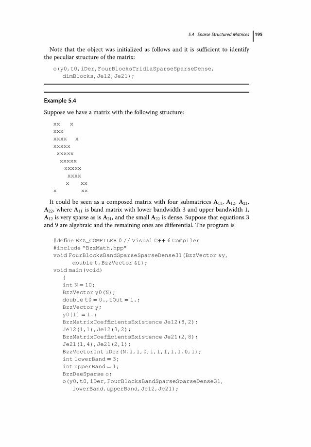
Note that the object was initialized as follows and it is sufficient to identifythe peculiar structure of the matrix:

o(y0,t0,iDer,FourBlocksTridiaSparseSparseDense,dimBlocks,Je12,Je21);

Example 5.4


xx xxxxxxxx xxxxxx

xxxxxxxxxx

xxxxxxxxx

x xxx xx

It could be seen as a composed matrix with four submatrices A11, A12, A21,A22, where A11 is band matrix with lower bandwidth 3 and upper bandwidth 1,A12 is very sparse as is A21, and the small A22 is dense. Suppose that equations 3and 9 are algebraic and the remaining ones are differential. The program is

#define BZZ_COMPILER 0 // Visual C++ 6 Compiler#include “BzzMath.hpp”void FourBlocksBandSparseSparseDense31(BzzVector &y,


{int N = 10;BzzVector y0(N);double t0 = 0.,tOut = 1.;BzzVector y;y0[1] = 1.;BzzMatrixCoefficientsExistence Je12(8,2);Je12(1,1),Je12(3,2);BzzMatrixCoefficientsExistence Je21(2,8);Je21(1,4),Je21(2,1);BzzVectorInt iDer(N,1,1,0,1,1,1,1,1,0,1);int lowerBand = 3;int upperBand = 1;BzzDaeSparse o;o(y0,t0,iDer,FourBlocksBandSparseSparseDense31,

lowerBand,upperBand,Je12,Je21);


y = o(tOut);o.BzzPrint(“Results”);double sum = y[1] + y[2] + 2.*y[3] + y[4] + y[10];BzzPrint(“\nSum %e”,sum);sum = y[4] + 2. * y[9] + y[10];BzzPrint(“\nSum %e”,sum);}

void FourBlocksBandSparseSparseDense31(BzzVector &y,double t,BzzVector &f)

{f[1] = 2.*y[1] + y[2] + y[9];f[2] = y[1] + 2.*y[2] + y[3];f[3] = y[1] + y[2] + 2.*y[3] + y[4] + y[10] - 1.;f[4] = y[1] + y[2] + y[3] + 2.*y[4] + y[5];f[5] = y[3] + y[4] + 2.*y[5] + y[6];f[6] = y[3] + y[4] + y[5] + 2.*y[6] + y[7];f[7] = y[5] + y[6] + 2.*y[7] + y[8];f[8] = y[5] + y[6] + y[7] + 2.*y[8];f[9] = y[4] + 2. * y[9] + y[10];f[10] = y[1] + 2.*y[10];}

Note that the object was initialized as follows and it is sufficient to identify thepeculiar structure of the matrix

o(y0,t0,iDer,FourBlocksBandSparseSparseDense31,lowerBand,upperBand,Je12,Je21);

Example 5.5


** ***** ***

** ***** ***

** ***** ***

** ***** ***

** +++***** +++***** +++***

** ***+++***** ***+++***** ***+++***


** ***+++***** ***+++***** ***+++***

** ***+++** ***+++** ***+++

It could be seen as a composed matrix with four submatrices A11, A12, A21,A22, where A11 is a diagonal block with block sizes 2× 2, A12 is a diagonal blockwith block sizes 2× 3, A21 is a diagonal block with block sizes 3× 2, and A22 is atridiagonal block with block sizes 3× 3. Suppose that equations 1–8 are algebraicand the remaining ones are differential. The program is

#define BZZ_COMPILER 0 // Visual C++ 6 Compiler#include “BzzMath.hpp”void FourBlockOne (BzzVector &y,


{int N = 20;int n1 = 2;int n2 = 3;BzzVector y0(N);y0 = 1.;BzzVectorInt indexOdeAlg(N);indexOdeAlg(1) = 0;indexOdeAlg(2) = 0;indexOdeAlg(3) = 0;indexOdeAlg(4) = 0;indexOdeAlg(5) = 0;indexOdeAlg(6) = 0;indexOdeAlg(7) = 0;indexOdeAlg(8) = 0;indexOdeAlg(9) = 1;indexOdeAlg(10) = 1;indexOdeAlg(11) = 1;indexOdeAlg(12) = 1;indexOdeAlg(13) = 1;indexOdeAlg(14) = 1;indexOdeAlg(15) = 1;indexOdeAlg(16) = 1;indexOdeAlg(17) = 1;indexOdeAlg(18) = 1;indexOdeAlg(19) = 1;indexOdeAlg(20) = 1;double t0 = 0.,tOut = 1.;BzzVector y;BzzDaeSparse o;


o(y0,t0,indexOdeAlg,FourBlockOne,N,n1,n2);y = o(tOut);o.BzzPrint(“Results”);}

void FourBlockOne(BzzVector &y,double t,BzzVector &dy)

{dy[1]= y[1] + y[9] + y[10] + y[11] - 4.;dy[2]=y[2] + y[9] + y[10] + y[11] - 4.;dy[3]=y[3] + y[12] + y[13] + y[14] - 4.;dy[4]=y[4] + y[12] + y[13] + y[14] - 4.;dy[5]=y[5] + y[15] + y[16] + y[17] - 4.;dy[6]=y[6] + y[15] + y[16] + y[17] - 4.;dy[7]=y[7] + y[18] + y[19] + y[20] - 4.;dy[8]=y[8] + y[18] + y[19] + y[20] - 4.;dy[9]=y[1] + y[2] - 2. * y[9] + y[10] + y[11];dy[10]=y[1] + y[2] + y[9] - 20. * y[10] + y[11];dy[11]=y[1] + y[2] + y[9] + y[10] - 5. * y[11];dy[12]=y[3] + y[4] - 8. * y[12] + y[13] + y[14];dy[13]=y[3] + y[4] + y[12] - 2. * y[13] + y[14];dy[14]=y[3] + y[4] + y[12] + y[13] - 2. * y[14];dy[15]=y[5] + y[6] - 2. * y[15] + y[16] + y[17];dy[16]=y[5] + y[6] + y[15] - 2. * y[16] + y[17];dy[17]=y[5] + y[6] + y[15] + y[16] - 3. * y[17];dy[18]=y[7] + y[8] - 2. * y[18] + y[19] + y[20];dy[19]=y[7] + y[8] + y[18] - 4. * y[19] + y[20];dy[20]=y[7] + y[8] + y[18] + y[19] - 12. * y[20];}

Note that the object was initialized as follows and it is sufficient to identify thepeculiar structure of the matrix:

o(y0,t0,indexOdeAlg,FourBlockOne,N,n1,n2);

Additional examples with different matrix structures forBzzDaeSparse, andBzzDaeSparseObject classes can be found in

BzzMath/Examples/BzzMathAdvanced/Dae

directory and

DaeSparseDaeSparseObject




5.5Industrial Case: Distillation Unit

Modeling of chemical processes lies at the foundation of any process systemsengineering activity, including design, control, optimization, planning, and retro-fitting. With the model designed to meet the specifications of the application,models according to their use and thus a multitude of models may be generatedfor the same plant, each serving a different purpose.Limiting the discussion to the use of first-principle models, the behavior of the

desired equipment is represented by either (i) a set of algebraic equations or (ii) asystem of ordinary differential equations (ODEs), or DAEs, or (iii) partial differen-tial equation (PDE) and partial differential–algebraic equation (PDAE), including

� mass, energy, and momentum balances;� transfer laws;� possible reactions;� thermodynamics, geometry, and so on;� secondary variables transformations; and� control laws.

Given the size, complexity, and coupling of these equations, solving themrequires a good, robust numerical solver that includes an integrator and possiblya local root solver.It is well known that solvers that exploit the sparse structure of its Jacobian are

more efficient in terms of CPU computation time than solvers that do not.Unfortunately, those solvers are not always available or applicable to the specificstudied case.For the purpose of discussing the different issues, let us consider the case of a

generic, binary distillation column (Manenti et al., 2009; Dones et al., 2010). It iswell known that first-principle distillation models (represented by a set of differ-ential and/or algebraic equations) have a sparse structure, well organized in tri-diagonal blocks (Naphtali and Sandholm, 1971). However, this nice structuremay be spoiled when control loops are introduced for the purpose of manipulat-ing the dynamic behavior of the plant. Control laws containing integral terms,such as PI and PID loops, introduce new states into the representation and thusnew equations to be integrated and, consequently, new elements that usually lieoutside the three-diagonal band into the Jacobian. The result is that solvers forsparse and well-structured DAE problems cannot be used directly for solvingthis type of problem. In practice, this means we often have to resort to a moregeneral solver, which is less efficient in terms of CPU time, or possibly evenaccept an approximate solution for the unstructured points in order to keepcomputational time short.On this subject, this section shows an efficient approach to precisely solve par-

tially structured DAE systems (Section 5.5.1), where an overall well-structuredJacobian is spoiled by a few unstructured elements.

5.5 Industrial Case: Distillation Unit 199

5.5.1

Management of System Sparsity and Unstructured Elements

Although advanced control and optimization methodologies have been exten-sively discussed in the scientific literature throughout the last three decades(Cutler and Ramaker, 1980; Morari and Lee, 1999; Manenti, 2011), conventionalcontrol systems are still the most commonly used approaches in the processindustry. In this framework, the integral part of each traditional control loop“corrupts” the Jacobian structure by introducing unstructured elements. Theseconsiderations make this example and, more specifically, the development ofbetter performing, tailored numerical solvers for partially structured systemshighly relevant.Actually, when the problem does not have a fully structured Jacobian (see

Figure 5.1), several very high-performance algorithms designed for sparse andwell-structured systems cannot be used.Several approaches can be adopted for solving the problem posed:

� The simplest way out is to use a generic DAE solver for dense systems ofequations. Unfortunately, the required CPU time increases exponentiallywith the size of the system as the algorithm does not take advantage of thesparsity of the system’s matrix.� Using a DAE solver that accepts the Jacobian existence matrix, that is, anincidence matrix only. This provides the solver with the possibility to com-pletely exploit the system’s sparsity, but not its overall structure. Neverthe-less, it is often not possible to provide the Jacobian incidence matrix,especially when the system is very large or when the incidence matrixchanges as part of an iterative process.� An approach that solves the unstructured part separately (e.g., quadrature ofthe integral), while the remaining sparse structure is efficiently calculatedwith an appropriate solver.

While this approach results in a significant improvement in com-putation time, the approximate solution may not be accurate enoughfor the application. Particularly, where control applications are con-cerned, these unstructured elements are related to the integral partof the control loops and an inaccurate solution may have cata-strophic effects mainly if the process is highly dynamic (e.g., surgelines and radicalic systems), where the correction selection of the dis-cretization time of the control action is also critical.� Alternatively, a novel generalized class of DAE solvers is generated with theobjective of simultaneously and efficiently solving the structured andunstructured part. A single DAE solver is then able to handle both the fullystructured problem and the corrupted structured problem containingunstructured elements (see Example 5.3).


5.5.2

DAE Solver for Partially Structured Systems

A novel approach was recently introduced to the BzzMath library (Manentiet al., 2009). A new DAE solver was created for very sparse systemscorrupted by a few unstructured elements, as they typically occur in the pro-cess control field. The implementation of this algorithm is now part ofBzzDaeSparse class.The matrix reproducing the Jacobian of Figure 5.1 can be rearranged as

reported in Figure 5.2, so as to obtain a matrix A that can be partitioned intofour blocks:

� A1;1 is a structured (i.e., diagonal, tridiagonal, tridiagonal blocks, staircase,etc.) submatrix. A necessary condition is that this matrix must be wellconditioned.� A1;2 and A2;1 are two (usually rectangular) sparse unstructured submatrices.� A2;2 is a generally dense submatrix.

XXX

XXX

XX

YY

YY

XX

YXXX

YXXX

Figure 5.1 Partially structured Jacobian: X-elements constitute a tridiagonal structure; Y-ele-ments are unstructured entries.

A1,1 A1,2

A2,1 A2,2

XX

YXXX

YXXX

XXX

XXX

XX

YYY

YYY

Figure 5.2 A1;1: structured (tridiagonal) block; A1;2 and A2;1: sparse unstructured blocks; A2;2:dense block.


The resulting four-blocks system is

A1;1x1 � A1;2x2 � b1 (5.2)

A2;1x1 � A2;2x2 � b2 (5.3)

which can be solved readily:

A1;1x1 � b1 � A1;2x2 (5.4)

A2;2 � A2;1A�11;1A1;2

� �x2 � b2 � A2;1A�1

1;1b1 (5.5)

Even though an inverse matrix appears in Equation 5.5, it is necessary to solvethe problem without explicitly inverting that matrix (Vol. 1, Buzzi-Ferraris andManenti, 2010a).To exploit the sparsity of unstructured submatrices, depending on the sparsity

degree of the two matrices A1;2, two alternative solving strategies are defined,which are similar in their evaluation of the product z � A�1

1;1b1, but proceedalong two parallel paths:

1) The product W � A�11;1A1;2 is evaluated through the solution of the system

A1;1W � A1;2. Once the matrix W is known, the following product is eval-

uated: A2;1A�11;1A1;2 � A2;1W. Then, the product A2;1z is computed and the

system (5.5) is solved for x2. Finally, the vector expression b1 � A1;2x2 isevaluated and the system (5.2) is solved for x1.

2) The product V � A2;1A�11;1 is evaluated by solving the equation AT

1;1VT �

AT2;1 for V. Once the matrix V is known, the product A2;1A�1

1;1A1;2 � VA1;2

is computed. Next, the product A2;1z is calculated and the system (5.5) issolved for x2. Finally, the vector b1 � A1;2x2 is evaluated and the system(5.2) is solved for x1.

The first alternative is used when the matrix A2;1 is sparse and the secondalternative is used when the matrix A1;2 is sparse. The algorithm exploitsthe sparsity and structure of matrix A1;1. It is consequently factorizedjust once.In addition to this, it is important to note that the matrix A2;1A�1

1;1A1;2 can beobtained column-by-column in the first case and row-by-row in the second case(Krishnamurthy and Taylor, 1985a; Krishnamurthy and Taylor, 1985b). The cal-culations can thus be done “in-memory” so that the matrix does not have to bestored, thereby reducing memory allocation.

5.5.3

Case-Study for Solver Validation: Nonequilibrium Distillation Column Model

A distillation column model was chosen to test the various solvers. First-princi-ple distillation models yield a tridiagonal block structure, each block


representing the properties of a single distillation stage (Dones et al., 2009). Afully dynamic model of an iso- and normal-butane splitter with control structureis shown in Figure 5.3.While the details of the model can be taken from the references (Dones et al.,

2009), a brief summary goes as follows: Each stage of the column is consideredas a nonequilibrium dynamic flash containment, where the liquid and gas phasesare two uniform lumps exchanging extensive quantities. The main differencesbetween it and traditional models are as follows:

� Dynamic mass and energy balance for both phases.� Gas capacity is included.� No chemical equilibrium assumption.� No thermal equilibrium assumption.� No assumption about the liquid density.

Figure 5.3 Distillation column flow-sheet and control scheme.


The dimension of the state is 2 �NC � 6 states per column stage, where NCstands for the number of components:

� NC dynamic liquid mass balances;� NC dynamic gas mass balances;� 1 dynamic energy balance for liquid phase;� 1 dynamic energy balance for gas phase;� 1 algebraic equation for liquid temperature calculation;� 1 algebraic equation for gas temperature calculation;� 1 algebraic equation for liquid volume calculation;� 1 algebraic equation for gas volume calculation.

Table 5.1 summarizes the system of equations given to the solver for thegeneric stage.The algebraic equations for temperatures and volumes are selected so as to be

solved directly by the DAE solver, since they are implicit equations and we preferto use a common numerical solver instead of tuning tolerances for internal andexternal loop solvers.The secondary variable transformations and all thermodynamic properties are

calculated using an external, portable, and easy-to-plug-in thermodynamic pack-age (Løvfall, 2008). The package accepts temperatures, volumes, and masses,returning Helmholtz’s energy and its derivatives with respect to the inputs.In this way, the liquid (or gas) pressure is calculated as a function of the liquid

(or gas) temperature, volume, and mass of that phase, as the pressure is the firstderivative of Helmholtz’s energy A with respect to temperature for a given vol-ume and mass, like in (5.6) and (5.7).

Table 5.1 Generic stage model.

Equations State

_nLi � �nLi�Li�1 � nLi�1�Li � nLi�Gi � nLi�env � nenv�Li Mass balance liquid phase nLi

_nGi � �nGi�Gi�1 � nGi�1�Gi � nLi�Gi Mass balance gas phase nGi

_ULi � �HLi�Li�1 � HLi�1�Li � qLi�Gi� HLi�Bi � qLi�Bi � pLi

_VLi

�HLi�env � Henv�Li � qLi�env � qenv�LiEnergy balance liquidphase

ULi

_UGi � �HGi�Gi�1 � HGi�1�Gi � qLi�Gi� HBi�Gi � pGi

_VGi Energy balance gas phase UGi

0 � ULi � UL�TLi ; VLi ;nLi � Calculate liquidtemperature

TLi

0 � UGi � UG�TGi ; VGi ;nGi � Calculate gas temperature TGi

0 � pLi � pGiMechanical equilibrium VLi

0 � VTOTi � �VLi � VGi � Volumes constraint VGi


@ALi

@VLi

��TLi ;nLi

� �pLi (5.6)

@AGi

@VGi

��TGi ;nGi

� �pGi(5.7)

The pressure drop along the column is not made explicit, but hidden in theresistance that the rising gas streams nGi�1�Gi have to face to flow up the column.The law defining nGi�1�Gi will be a valve-like equation, and thus contain the pres-sure drop in the form of dry and wet tray resistances. This is somewhat differentfrom Krishnamurthy and Taylor (1985a, 1985b) where, in order to express thecolumn pressure drop as a function of tray (or packing)-type, a hydraulic equa-tion must be considered for each day and the pressure drop of each stage mustbe made into an unknown (and therefore explicit) variable. Krishnamurthy andTaylor pointed out that many numerical solution methods (e.g., the Newtonmethod for the solution of algebraic systems) require derivatives, and some ofthem may be unavailable (with respect to thermodynamic and transport propert-ies). They thus urged the user to adopt approximations when required. HavingLøvfall’s (2008) stand-alone thermo modules available makes any numericalapproximation obsolete. Derivatives are computed from analytically derivedexpressions within those modules, thus making them incredibly flexible for usein advanced algorithms. The implemented controllers are feedback controllers.On the top and bottom, the product streams are supervised by a proportionalcontroller to maintain the desired liquid level in the respective drums. The col-umn is also equipped with a proportional-integral pressure control, whichrestricts the gas stream to the condenser to regulate the top pressure of the split-ter. Finally, there is a proportional-integral temperature controller implementedto control the temperature in the lower section by manipulating the reboiler duty.Adding two PI controllers to the set of equations increases the number of

dynamic equations the DAE solver must integrate by 2 and inserts 14unstructured elements into the well-structured tridiagonal block Jacobian, asshown in Figure 5.4.The Jacobian is still highly sparse, even though the few elements in the ellipses

corrupt the compact tridiagonal structure.

5.5.4Numerical Results

In order to measure the performance of the new algorithm, two solvers are beingused, namely, the full scheme and the advanced sparse solver. The distillationmodel is excited with an external input. Three cases were generated:

1) Procedure A: BzzDae is used to solve the system. Neither structure norsparsity information is provided.


2) Procedure B: BzzDaeSparse is used. Information about the overall Bool-ean Jacobian (incidence matrix) is provided.

3) Procedure C: The new BzzDaeSparse is used, providing informationabout the structure of the partially structured system. The location of theunstructured elements must also be provided.

Distillation column models are well known to be nonlinear. This implies that a+10% step perturbation in the feed composition could display different dynamicsand nonsymmetrical responses to a �10% step perturbation. Six different inputsequences were studied and in each case, the computational time for computingthe process transient was recorded, for both the open- and closed-loopconfigurations.Starting from the steady-state conditions, step variations were introduced into

the system at time zero: the first 6 s of simulation were in open-loop configura-tion, and thereafter for 24 s, the control loops were closed, with a sampling timeof 6 s. Only this highly dynamic regime was chosen since the solvers performnearly the same when the process is close to steady state, and choosing longersimulation times will not suffice to measure the solvers’ performances.The following six-step variations were introduced into the feed composition of

isobutane with respect to the nominal value: ±10, ±20, and ±50%.Tables 5.2 and 5.3 summarize the computation times (in seconds) required for

the three procedures with the six-step perturbations.

Figure 5.4 Partially structured tridiagonal block Jacobian. The points in row 941 and 942 andin column 941 and 942 represent the unstructured elements: Specifically, the circles are ele-ments of matrices A1;2 and A2;1, while the diamonds belong to the matrix A2;2.


It is well known that a method accounting for system sparsity is much fasterthan methods that do not. Looking at the results, this trend is confirmed. Actu-ally, procedure A, which solves the system without any sparsity information,requires about 8 s to simulate 6 s in open-loop and about 23 s to simulate theremaining 18 s of closed-loop scenario on an Intel CoreTM 2 Duo CPU,2.00GHz, 2.00GB of RAM. The integration is rather time-consuming and itdoes not allow any application of predictive techniques and moving horizonmethodologies, which requires online feasibility and faster than real-time CPUintegration times.Conversely, procedure B, where the user has to define the whole existence of

Jacobian matrix, is generally four times faster than procedure A. It requiresabout 2 s to simulate 6 s in open-loop and about 3.5 s to simulate the closed-loop scenario.In turn, procedure B is four times slower than procedure C for all the step

input signals studies, as the latter does not only exploit the system sparsity andstructure, but also the location of the unstructured nonzero elements. By adopt-ing the partially structured DAE solver, one needs half a second to simulateopen-loop scenarios and about 1s for the closed-loop ones.The type of disturbance does not affect computation time, even though there

are three outliers in open-loop calculations, as reported in Table 5.2. A �50%disturbance requires more or less twice the CPU time taken by the other stepinputs in procedures A and C, while +10% in procedure C is about three timesslower than the time consumed by the other implemented step disturbances.

Table 5.2 CPU time comparison, open-loop (in seconds).

Disturbances Procedure A Procedure B Procedure C

+10% 7.92 5.89 0.47�10% 7.86 1.89 0.44+20% 7.91 1.92 0.47�20% 7.92 1.92 0.48+50% 7.98 2.16 0.52�50% 15.78 2.16 0.94

Table 5.3 CPU time comparison, closed-loop (in seconds).

Disturbances Procedure A Procedure B Procedure C

+10% 22.67 3.13 0.95�10% 22.61 3.33 0.97+20% 22.69 3.33 0.97�20% 22.70 3.56 0.97+50% 22.73 3.38 1.00�50% 22.81 3.59 1.06


This is mainly due to the size of the integration steps, which is automaticallydefined by the stiff solvers and strongly nonlinear process dynamics. When thesystem is operating in a closed-loop scenario, controllers are able to stabilizeprocess dynamics and, consequently, prevent any possible less high-performancesolutions in terms of CPU requirements.A high-performance algorithm to solve DAE systems with sparse Jacobian,

whose elements are partially structured, was proposed and applied to an indus-trial case. This is a common case in process modeling and control applications,since the integral term of conventional control loops is usually an unstructuredelement that may spoil the overall well-defined system structure. In this regard,existing solvers cannot completely exploit either the system structure or, attimes, the system sparsity, leading to an unavoidable increase of the computa-tional time. However, the novel approach developed and implemented in theBzzMath library can exploit the overall structured morphology of the system byrequiring only a small amount of extra information about the unstructured ele-ments. It allows a significant improvement in the computation time of numericalDAE system integrations, comparable with the numerical improvement betweendense and sparse solvers in the solution of fully structured systems.

Notations for Table 5.1

n NC dimensioned mass vectorU internal energyT temperatureV volumep pressureq heatH enthalpy

Subscripts

i stage position (counting from the top)L liquid phaseG gas phaseB boundary between liquid and gas phaseTOT stage propertyenv external environment

Symbols

^ stream;� time derivative


6Boundary Value Problems


6.1Introduction

This chapter deals with the problem of integrating a system of N ordinary differ-ential equations:

f y´´; y´; y; x� � � 0 (6.1)

in the interval xA; xB� � with boundary conditions

x � xA; gA y´´ xA� �; y´ xA� �; y xA� �; xA� � � 0 (6.2)

x � xB; gB y´´ xB� �; y´ xB� �; y xB� �; xB� � � 0 (6.3)

The vector of the variables y is dimensioned N or N � 1. When the number ofvariables is dimensioned N � 1, one of them is a constant parameter that has tobe evaluated by solving the problem (see Section 6.1.3).

The problem of integrating a system of differential or algebraic–differentialequations with boundary conditions is indicated with the acronym BVP.

The following are some of the important observations:

� We assumed that second derivatives y´´ are present in the problem formula-tion. This decision relates to the fact that these derivatives are present inmany practical problems.� In some problems, there may be higher order derivatives. This, however, israre and usually with a reduced number of variables. If the problem is

209



explicit, it is trivial to transform it into the form (6.1)–(6.3) by using novelvariables and equations. For example, consider the problem

u´´´ � h u´´; u´; u; x� � (6.4)

By introducing the variables

y1 x� � � u x� � (6.5)

y2 x� � � u´ x� � (6.6)

the problem becomes

y1 � y2y´2 � h y2; y1; y1; x

� � (6.7)

which enters the types (6.1)–(6.3) broached here.� The boundary conditions considered in this chapter are assigned to only twopoints. Thus, we will not consider those problems where the boundary con-ditions are assigned to many points:

x � xA; gA y´´ xA� �; y´ xA� �; y xA� �; xA� � � 0 (6.8)

x � xB; gB y´´ xB� �; y´ xB� �; y xB� �; xB� � � 0 (6.9)

x � xC ; gC y´´ xC� �; y´ xC� �; y xC� �; xC� � � 0 (6.10)

� The boundary conditions in the two points are only functions of the varia-bles and of their first and second derivatives in xA and xB, respectively.

Therefore, we will not consider those problems where the conditions are simul-taneously functions of the value of the variables and their first and second deriv-atives in both points.

For example,

g y xA� �; y xB� �� 0 (6.11)

When the boundary conditions are in the forms (6.2) and (6.3), they are denotedas disjoined boundary conditions.

It is worth noting that in both cases it is always possible to refer readers to thecase considered in the chapter by adding an adequate number of equations andvariables. For example, consider the problem

h u´´; u´; u; x� � � 0 (6.12)

subject to the conditions

b11u xA� � � c1 (6.13)

b21u xA� � � b22u xB� � � c2 (6.14)

210 6 Boundary Value Problems

By introducing the variables

y1 � u (6.15)

y2 � const � b21y1 xA� � (6.16)

the problem becomes

h y´1 ; y1; y1; x� � � 0 (6.17)

y2 � 0 (6.18)

with the conditions

b11y1 xA� � � c1 (6.19)

b21y1 xA� � � y2 xA� � � 0 (6.20)

b22y1 xB� � � y2 xB� � � c2 (6.21)

which enter the category considered in this chapter.

We will suppose that the independent variable x is continuous in the intervalxA; xB� � and that the corresponding components of y are also continuous withinsuch an interval. Usually but not necessarily, the first derivatives of y are also con-tinuous. Possible discontinuities in the first derivatives must be known a priori.

The problem of integrating a system of differential equations with boundaryconditions is harder to solve than problems with initial conditions.

Of the various difficulties that may arise, it is worth remarking that this problemcould have either one solution or multiple solutions (infinite solutions even), orno solutions.

For example, consider the problems

y´´ � y � 0y 0� � � 0y xB� � � b

(6.22)

The solution that satisfies the first boundary condition is

y x� � � C � sin x� � (6.23)

The constant C must be calculated so as to satisfy the second boundary condi-tion: If xB � nπ and b ≠ 0, the problem is infeasible; if xB � nπ and b � 0, theproblem has infinite solutions; and if xB � 0:5 and b � sin 0:5� �, the problem hasa unique solution for C � 1.

6.1.1

Integral Relationships

In some problems, an integral of the following type may be present:

I � ∫xB

xA

q y x� �; x� �dx (6.24)


Two different situations must be considered:

� The value of I is unknown and therefore the integral must be calculated.� The value of I is assigned and in this case the integral constitutes a specialboundary condition.

In the former case, the following strategies can be adopted:

� The integration is performed when the problem has been solved and thevalues of y are known in the support points.� The integration is performed during the search by inserting a new variableyN�1, a new equation, and a new boundary condition.

yN�1 � q y x� �; x� �yN�1 xA� � � 0

(6.25)

In this case, the value of I is obtained by making it equal to yN�1 xB� �. Con-versely, when I is assigned, it is possible to adopt the following strategy. A newvariable, yN�1, is inserted together with a new equation and two new boundaryconditions:

yN�1 � q y x� �; x� �yN�1 xA� � � 0

yN�1 xB� � � I

(6.26)

6.1.2

Continuation Methods

Many of the algorithms used to solve a BVP lead to the solution of a nonlinearalgebraic system in the unknown v.For reasons that will be explained later, it is opportune to formulate the sys-

tem using a vector z of M parameters:

w v; z� � � 0 (6.27)

The system must be solved with respect to the variable v for an assigned value ofthe parameter z � zF . Suppose we know another system q v; z� �, which is also relatedto (6.27) and easy to solve with respect to the variable v with assigned z; in this casea new system, a linear combination of the previous two systems, can be written:

h v; z; t� � � t � w v; z� � � 1 � t� �q v; z� � � 0 (6.28)

The parameter t in the relation (6.28) is called the homotopy.

By varying it in the range 0; 1� �, the system h is solved for a value of v thatsimultaneously satisfies the systems q and w.


The parameter z can be related to the parameter t in different ways on condi-tion that z � zF at t � 1. The simplest relationship is linear:

z � z0 � zF � z0� � � t (6.29)

where z0 is the initial value of the parameters. Another relationship usuallyadopted is

zi � z0izFiz0i

� �t

(6.30)

There are different choices for the system of auxiliary equations q v; z� � andtheir common feature is that for t � 0, the solution of the following system mustbe easy:

q v0; z0� � � 0 (6.31)

The main selections are

1) Homotopy with fixed point: q v; z� � � v � v0� � � z � z0� �:h v; z; t� � � t � w v; z� � � 1 � t� � v � v0� � � z � z0� �� 0 (6.32)

2) Newton or global homotopy: q v; z� � � w v; z� � � w v0; z0� �:h v; z; t� � � w v; z� � � 1 � t� �w v0; z0� � � 0 (6.33)

3) Parametric continuation method: q v; z� � � 0:

h v; z; t� � � w v; z� � � 0 (6.34)

This last criterion deserves some detailed explanation since it might seem thatthe problem of solving the nonlinear system has not been modified.In many practical cases, a problem could have a simple solution to be obtained

in correspondence with a vector of parameter z0, whereas numerical issues arisewhile achieving the required value zF . In this case, the system is first solved att � 0 and in this way, we obtain a value v0 such that

h v0; z0; 0� � � w v0; z0� � � 0 (6.35)

Subsequently, t is modified from 0 to 1 so as to allow the parameters to passfrom z0 to zF with continuity and the intermediate problems are solved.For example (see Example 6.8), Ascher et al. (1987) proposed the following

problem:

z 1 � x2� �

yy´´ � 1:2 � 2zx� �yy´ � y´y� 2x1 � x2

1 � 0:2y2� � � 0

y 0� � � 0:9129

y 1� � � 0:375

z � 4:792 � 10�8

(6.36)


The equation could present numerical issues with many algorithms due to thesmall value of z. The problem can be solved by varying with continuity theparameter z, for instance, from 10�2 to the desired value.

6.1.3

Problems with an Unknown Constant Parameter

Occasionally, an unknown constant parameter may be present in certain equa-tions in the system. Since such a parameter must be determined too, this givesrise to an additional boundary condition on one of the equations; a commonexample is when a variable is included in an equation with the first derivativeonly and that equation has two boundary conditions.This parameter differs from the other variables of the system for the following

reasons:

� It is constant on the overall interval.� There is no equation related to the same parameter, contrary to what hap-pens with the other variables of the system.

The easiest way to insert the unknown value of a parameter is to add a slackdifferential variable

dyN�1dx

� 0 (6.37)

which shows the constant value of the parameter within the interval.

6.1.4

Problem with Unknown Boundary

In some problems, one of the extremes of the interval is unknown. An additionalcondition must be introduced in this case also to allow its determination.This problem can be brought back to the determination of an unknown

parameter by inserting a new variable defined as the difference between theunknown extreme of the interval, for instance xB, and the beginning of the inter-val, xA:

yN�1 � xB � xA (6.38)

Moreover, the integration variable x is changed, using the variable t defined as

t � x � xAxB � xA

(6.39)

Now the system must be integrated between the known extremes 0 and 1 withrespect to t, whereas the variable yN�1 is an unknown constant parameter.

Also, in the case of problems with an unknown boundary problem, we can havezero, one, or infinite solutions.


For instance, consider the problem of finding the value of xB such that by inte-grating the differential equation

dydx

� �y (6.40)

the following conditions are satisfied: y 0� � � 1 and y xB� � � 0:5.The problem has a unique solution: xB � �ln 0:5� �.Conversely, consider the problem of finding the value of xB such that by

integrating the differential equation

d2ydx2

� �y (6.41)

the following conditions are satisfied: y 0� � � 0, y´ 0� � � 1, and y xB� � � μ. If μ � 2,the problem is infeasible; if μ � 1, it has infinite solutions.

6.2Shooting Methods

In Chapter 2, we saw that many algorithms allow the efficient solution of theproblem of integrating a system of differential equations:

y´ � f t; y� �; 0 < t < b (6.42)

when the conditions are in correspondence with the initial point

y 0� � � y0 (6.43)

It is therefore possible to think (and actually many authors have spent timetackling the problem this way) of providing the missing conditions as the initialguess, integrating the system using one of the above-mentioned algorithms, andusing the conditions assigned to the other extreme of the interval to correct theinitial condition just introduced. In other words, the problem is thus trans-formed into a zeroing of a system of equations (Vol. 3, Buzzi-Ferraris and Man-enti, 2014).

The name shooting methods comes from the fact that this procedure is similar totrying to hit a specific target by changing the aim of a gun.

For physical reasons, in almost all real problems where some conditions areassigned at the beginning of the integration interval and the remaining ones atthe end of it, the direction in which the corresponding equations are well con-ditioned is for increasing t in the first case and the opposite direction in thesecond case.

Thus, some equations are ill-conditioned when the integration starts from theinitial point, providing the missing initial conditions, and some others are ill-conditioned when the integration starts from the final point, providing the

6.2 Shooting Methods 215

missing boundary conditions. In these cases, it is very difficult, if not impossible,to solve the corresponding system.

By way of example, consider the following systems:

dy1dt

� �λy1 (6.44)

dy2dt

� λy2 (6.45)

with boundary conditions

y1 0� � � 1 (6.46)

y2 1� � � 1 (6.47)

Suppose we provide the values y1 0� � � 1 and y2 0� � � 5:297353e-022, which arein practice the exact values when λ � 50, and suppose we integrate the system inthe interval t � 0; 1� �. The second equation is ill-conditioned if integrated forincreasing t; if the value of λ is sufficiently large, that is, λ � 50, the solution ofthe second equation diverges from the exact solution, as reported in Figure 6.1.On the other hand, if we provide the values y1 1� � � 5:297353e-022 and y2 1� � �

1 and integrate the system from t � 1 to t � 0, the first equation is ill-condi-tioned. If the value of λ is still λ � 50, then the solution of the first equationdiverges from the exact solution (Figure 6.2).As already mentioned, this fact is often related to a physical feature of the

equation to which boundary conditions have been assigned. Such an equation iswell conditioned only if it is integrated starting from the point where the condi-tion is assigned and ill-conditioned if integrated in the opposite direction.

Figure 6.1 Trend of variables y1 and y2 in forward integration.


In nonlinear problems, an additional issue may arise: By integrating the systemstarting from initial conditions different from the correct ones, the solutioncould exist only in a subinterval xA; xC� � of the original interval with xC < xBand therefore the integration cannot be concluded.

Except for some particular cases, the methods based on this technique presentinsurmountable issues.

Clearly, the longer the integration interval, the greater the numerical diffi-culties. Many authors have tried to split the integration interval into anappropriate number of subintervals, resulting in the so-called multiple shoot-ing approach.

Rather than solving a single nonlinear system dimensioned as the missing initialconditions, each subinterval introduces an even number of variables and equa-tions into the overall system.

In the BzzMath library, the multiple shooting algorithms have not been imple-mented in a dedicated class.

6.3Special Boundary Value Problems

Let us consider the special problem where the system is explicit in the firstderivative:

y´ � f t; y� �; tA < t < tB (6.48)

Figure 6.2 Trend of variables y1 and y2 in backward.

6.3 Special Boundary Value Problems 217

subject to N � NA � NB two-point boundary conditions

gA yA; tA� � � 0; gB yB; tB

� � � 0 (6.49)

Very often the relations (6.49) are

yA tA� � � yA; yB tB� � � yB (6.50)

This formulation is adopted by many authors, but presents some deficiencies.

1) While this situation occurs frequently in differential systems with initialconditions, it does not when the conditions are assigned at different points.

2) To transform a system with second derivatives into a problem with onlyfirst derivatives, the number of variables is doubled. This is not a problemwhen the number of variables is rather small but it becomes relevant inlarge-scale systems.

3) First and second derivatives are implicit in many practical problems and itis not possible to transform the original system.

4) Also, when the transformation is feasible, it may be unsuitable to perform(Ascher et al., 1987). In fact, the new problem formulation may be ill-conditioned, whereas the original form were not.

5) It requires the user to know several tricks useful to transforming the prob-lem into the most favorable forms (6.48) and (6.49) (Ascher and Petzold,1998).

Notwithstanding all of these, there are some problems where such a formulationis adequate and it is suitable to exploit its particular structure, which allows it touse dedicated algorithms unsuited to general case.

6.3.1

Runge–Kutta Implicit Methods

While in the case of ODE with initial conditions the multivalue methods are verypromising also for stiff systems, in the special case of BVP here considered theimplicit Runge–Kutta methods are the most performing ones.

In the BVP, it is not possible to exploit the calculation history since all the ymust be simultaneously evaluated for all the intervals.

While in the case of ODE with initial conditions k of the explicit algorithms donot require any nonlinear system solution, this is no longer true for BVP. It istherefore reasonable to adopt implicit algorithms that are preferable in terms ofstability.

Of the most common implicit algorithms, the most useful ones are thoseadopting quadrature points, which are points used by the open Gauss method,semiopen Radau method, and the close Lobatto method (see Chapter 1).Two implicit Runge–Kutta algorithms in particular are very widely used: One

is derived from the Gauss’s rule with one point only (equivalent to the middle


point method) and the other from Lobatto’s rule with three points (equivalent tothe Cavalieri–Simpson’s rule).Runge–Kutta’s method derived from the Gauss method with one intermediate

point only is

k1n � hnf yn � k1n2

; tn � hn2

� �(6.51)

yn�1 � yn � k1n (6.52)

This is a method of the second order.If we evaluate k1n from (6.52) and replace it in (6.51), the result is

yn�1 � ynhn

� fyn � yn�1

2; tn � hn

2

� �(6.53)

Lobatto’s method with three points is similar to Cavalieri–Simpson’s method,where the three points are at the extremes and in the center of the interval. Thecorresponding Runge–Kutta’s method is

k1n � hnf yn; tn� �

(6.54)

k2n � hnf yn � 524

k1n � 13k2n � 1

24k3n; tn � hn

2

� �(6.55)

k3n � hnf yn � 16k1n � 2

3k2n � 1

6k3n; tn � hn

� �(6.56)

yn�1 � yn � 16k1n � 2

3k2n � 1

6k3n (6.57)

This is a fourth-order method. In this case too, it is possible to obtain

k3n � hnf yn�1; tn�1� �

(6.58)

by means of the relation (6.57) and also obtain the following using (6.55) and(6.56):

yn�1 � ynhn

� 16

�f�tn; yn� � f�tn�1; yn�1�

� 4fyn � yn�1

2� hn

8f�tn; yn� � f�tn�1; yn�1��

; tn � hn2

� �(6.59)

The structure of the resulting system is very favorable in both the cases. Sup-pose we have N equations and split the interval into M subintervals. A total ofN M � 1� � variables is obtained and the nonlinear system has the following struc-ture, exemplified for N � 3 and M � 5 in case of two initial conditions and onefinal condition.

6.3 Special Boundary Value Problems 219

**

xx*xxxxxx*xxxxxx*x

xx*xxxxxx*xxxxxx*x

xx*xxxxxx*xxxxxx*x

xx*xxxxxx*xxxxxx*x

xx*xxxxxx*xxxxxx*x

*

These methods present the following pros and cons.

1) They lead to a nonlinear system with very favorable structure.2) They are symmetric. This feature is very important especially for problems

that are not overly stiff. Actually, unlike the integration of systems withinitial conditions, ill-conditioning issues may arise when integrating forincreasing and decreasing t.

3) They are A-stable methods.

1) They are not strongly A-stable. They could have numerical issues with verystiff equations.

2) They require the system in the forms (6.48) and (6.49).

There are several very useful tricks for the implementation of these algo-rithms. The first one is a preventive pivoting: The variables must be swappedso as to have as first variables those with initial conditions assigned in tA.The first and last equations are initial and final conditions, whereas theremaining Equation 6.53 or 6.59 must be swapped to have as the first set theequations that refer to the conditions assigned at the final point tB, followedby the equations related to the conditions assigned at the initial point tA.Two advantages are obtained.

1) It is possible to solve the linearized system (required to solve the nonlinearsystem with the Newton method) in an efficient way using staircase factor-ization with limited row swapping.

2) Equation 6.53 or 6.59 is often solved in a more stable manner since thosewith initial conditions are solved using increasing t and those with finalconditions by using decreasing t.


There is one additional trick that will help effectively solve the nonlinearsystem:

� To build the Jacobian, it is possible to vary several variables simultaneouslyby exploiting the structure of the system (see Section 2.16.2.4).If several processors are available, further tricks could be exploited:� Since the calculation of the residuals is carried out when all the variables yn are

known, it is possible to calculate the vectors f yn; tn� �

using parallel computing.� Finally, the factorization of the linear system can also be solved using paral-lel computing.

In the BzzMath library, these algorithms have not been implemented in dedi-cated classes.

6.4More General BVP Methods

Suppose for the sake of simplicity we have a single differential equation

f y´´; y´; y; x� � � 0 (6.60)

which has to be integrated in the interval xA; xB� � with the following boundaryconditions:

x � xA;gA y´´ xA� �; y´ xA� �; y xA� �; xA� � � 0

(6.61)

x � xB;gB y´´ xB� �; y´ xB� �; y xB� �; xB� � � 0

(6.62)

Let us indicate with v a; x� � an opportune function with P, adaptive parameters a,and with v´ a; x� � and v´´ a; x� � the first and second derivatives, respectively, obtainedanalytically with respect to the variable x. By introducing the function v and itsderivatives into the differential equation and in the boundary conditions, we obtain

R a; x� � � f v´´ a; x� �; v´ a; x� �; v a; x� �; x� � ≠ 0 (6.63)

gA v´´ a; xA� �; v´ a; xA� �; v a; xA� �; xA� � ≠ 0 (6.64)

gB v´´ a; xB� �; v´ a; xB� �; v a; xB� �; xB� � ≠ 0 (6.65)

The function R a; x� � is called the function of residuals.

Traditionally, all the methods that adopt the approximate functions v a; x� � arebrought back to a single criterion: the method of weighted residuals, accordingto which the P conditions needed to evaluate the P parameters are

∫xB

xA

WkR a; x� �dx � 0; k � 1; . . . ;P (6.66)

6.4 More General BVP Methods 221

with R a; x� � the residual obtained by including the adaptive functions in the sys-tem of differential equations to be solved. The various methods differ accordingto the selection of the weights Wk that appear in the integrals and, for each ofthem, one or two equations must be replaced with the relative boundarycondition.

For the sake of simplicity, the methods are described by assuming the intervalxA; xB is not split into elements, but is instead considered a single element.

6.4.1

Collocation Method

With the collocation method, Dirac’s delta function is used as the weight func-tion in the support point xk :

Wk � δ x � xk� �; k � 2; . . . ;P � 1 (6.67)

The nonlinear system becomes

gA v´´ a; xA� �; v´ a; xA� �; v a; xA� �; xA� � � 0 (6.68)

R a; xk� � � f v´´ a; xk� �; v´ a; xk� �; v a; xk� �; xk� � � 0; k � 2; . . . ;P � 1 (6.69)

gB v´´ a; xB� �; v´ a; xB� �; v a; xB� �; xB� � � 0 (6.70)

There are really many different variants of this method based on the selec-tion of the support points and the elements to discretize the interval. Someof them have special names that highlight their approach. For instance, if thepoints are selected as the roots of an orthogonal polynomial and if the ele-ments have only one point in common, the method is said to be a finite-ele-ment orthogonal collocation. On the other hand, if each element consists ofthree points and the adjacent elements share two points, the method is saida finite-difference method. In some cases, when the elements have commonpoints, the single residual is not zeroed, but the sum of residuals is calculatedin the same point using all the elements that are sharing it. The aim of thesevariants is to find a well-conditioned system of equations with a structurethat makes its solution particularly efficient when the number of variables israther large.

6.4.2

Galerkin Method

In the Galerkin method, the derivatives of the function v a; x� � with respect to theunknown parameters are adopted as weights:

Wk � @v a; x� �@ak

; k � 2; . . . ∞ ;P � 1 (6.71)


There is a theoretical reason why the Galerkin method is selected, but we donot explore it in depth in this book. The nonlinear system becomes


∫xB

xA

@v a; x� �@ak

R a; x� �dx � 0; k � 2; . . . ;P � 1 (6.73)


The Galerkin method is particularly efficient for some special structuredboundary value problems (Burnett, 1987).

6.4.3

Momentum Method

In this method, the weight functions are the increasing powers of x:

Wk � xk�1; k � 1; . . . ;P � 2 (6.75)



∫xB

xA

xk�1R a; x� �dx � 0; k � 1; . . . ;P � 2 (6.77)


6.4.4

Least-Squares Method

Two versions of this method can be quoted: the traditional one that enters thisfamily and an alternative that, conversely, does not belong to it.The first alternative uses the following weights:

Wk � @R@ak

; k � 2; . . . ;P � 1 (6.79)



∫xB

xA

@R a; x� �@ak

R a; x� �dx � 0; k � 2; . . . ;P � 1 (6.81)


6.4 More General BVP Methods 223

This system represents the necessary conditions such that the following inte-gral is minimum:

I � ∫xB

xA

R2 a; x� �dx (6.83)

The second alternative searches for the minimum of the integral directly usinga multidimensional minimization method subject to the boundary equationswith respect to the P unknown a.

6.5Selection of the Approximating Function

The method adopted aside, the approximation function v can be selectedaccording to three strategies.

1) The function v satisfies both the boundary conditions for each value of a.2) The function v satisfies one boundary condition for each value of a.3) The function v does not automatically satisfy the boundary conditions.

The first two strategies are used to solve special problems. For instance, if thetwo boundary conditions are

x � 0; y 0� � � yA (6.84)

x � 1; y 1� � � yB (6.85)

the following function automatically satisfies them for each value of a:

v � yA � x yB � yA� � �XP

i�1ai x

i�1 � x� �

(6.86)

From a general viewpoint, it is suitable to take into consideration the thirdstrategy. It is clear that in such a case it is necessary to use a method that canself-select the parameters a of the model v a; x� � so as to satisfy at best theboundary conditions.Also from a general viewpoint, it is opportune that the function v a; x� � that

approximates y and contains P adaptive parameters a has the following features.

1) Whatever the value of x and a, if required, the corresponding values of v,v´, and v´´ must be easy to obtain.

2) The adaptive parameters a must be easy to obtain once the support pointsxi; yi are assigned.

If the Galerkin method is adopted, the first derivative of v with respect to allthe adaptive parameters must also be easy to evaluate.

The most obvious selection, which is also adopted here, is a P � 1� �-degree poly-nomial with P being the number of unknown adaptive parameter a.


6.6Which and How Many Support Points Have to Be Considered?

At first glance it would seem ideal to use a single polynomial of opportune gradethat can approximate the solution for the overall interval.

However, it is an error to believe that the approximation of a function alwaysimproves as the polynomial degree increases. This happens only if some propertechniques are adopted (see Vol. 2, Buzzi-Ferraris and Manenti, 2010b).

The previous observation is especially valid if the support pointsx1; x2; . . . ; xP�1; xP (with x1 � xA and xP � xB) are either evenly spaced orselected without the appropriate precautions. The approximation stronglyimproves by opportunely selecting the internal points x2; . . . ; xP�1.

Except for some very favorable cases that will not be considered here, it is notopportune to use a single polynomial to approximate the function. It is thereforepreferable to split the interval into a series of subintervals, which will be calledthe elements, and to calculate the approximating polynomial for each of themusing the support points of such a subinterval.

Two strategies are possible for the selection of the elements:

� The adjacent elements have two or more common support points.� The adjacent elements have one single common support point.

In the first case, the two adjacent elements are partially overlapped, whereas inthe second case the last support point of the element coincides with the firstsupport point of the next element.

In the following, we will suppose that every element has the same number ofsupport points, P, for the sake of simplicity and we will indicate with K � P � 2the number of internal support points for each element and with E the numberof elements.

First strategy: The adjacent elements have two or more common supportpoints.If two adjacent elements have only two common support points, the series of

support points will be x1 � xA; x2; . . . ; xP belonging to the first element,xP�1; xP; xP�1; . . . ; x2P�2 belonging to the second element, x2P�3; x2P�2; . . . ; x3P�4belonging to the third element, and so on. The total amount of support points isE � K � 2 � E P � 2� � � 2.For instance, in the case of four support points for each element and three

elements, the points x1; x2; x3; x4 with x1 � xA belong to the first element, thepoints x3; x4; x5; x6 belong to the second element, and the points x5; x6; x7; x8 �xB belong to the third element (Figure 6.3).On the other hand, if two adjacent elements have P � 1 common support

points, the series is x1 � xA; x2; . . . ; xP belonging to the first element,

6.6 Which and How Many Support Points Have to Be Considered? 225

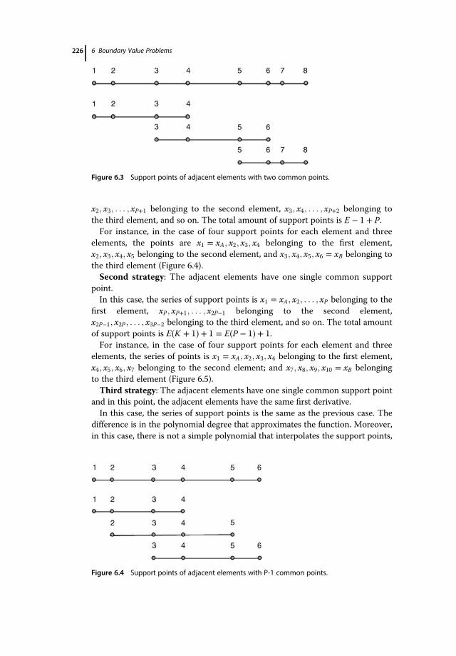
x2; x3; . . . ; xP�1 belonging to the second element, x3; x4; . . . ; xP�2 belonging tothe third element, and so on. The total amount of support points is E � 1 � P.For instance, in the case of four support points for each element and three

elements, the points are x1 � xA; x2; x3; x4 belonging to the first element,x2; x3; x4; x5 belonging to the second element, and x3; x4; x5; x6 � xB belonging tothe third element (Figure 6.4).Second strategy: The adjacent elements have one single common support

point.In this case, the series of support points is x1 � xA; x2; . . . ; xP belonging to the

first element, xP; xP�1; . . . ; x2P�1 belonging to the second element,x2P�1; x2P; . . . ; x3P�2 belonging to the third element, and so on. The total amountof support points is E K � 1� � � 1 � E P � 1� � � 1.For instance, in the case of four support points for each element and three

elements, the series of points is x1 � xA; x2; x3; x4 belonging to the first element,x4; x5; x6; x7 belonging to the second element; and x7; x8; x9; x10 � xB belongingto the third element (Figure 6.5).Third strategy: The adjacent elements have one single common support point

and in this point, the adjacent elements have the same first derivative.In this case, the series of support points is the same as the previous case. The

difference is in the polynomial degree that approximates the function. Moreover,in this case, there is not a simple polynomial that interpolates the support points,

Figure 6.3 Support points of adjacent elements with two common points.

Figure 6.4 Support points of adjacent elements with P-1 common points.


but a Hermite polynomial (Vol. 2, Buzzi-Ferraris and Manenti, 2010b) where thefirst derivatives at the extremes support points are also assigned.

Whatever strategy is adopted, the number of support points in each elementmust be small (three or four, for instance) when their position inside the elementis inappropriately selected.

Thus, using the first strategy in the case of two shared support points, itis possible to select between two alternatives: the elements have differentdimensions and the support points are not efficiently selected or the ele-ments have the same dimension and the support points are efficientlyselected, but evenly spaced inside each interval. The first alternative is suit-able since it could be useful to intensify the elements of small dimensionsat the critical points of the problem solution; conversely, the second alter-natives ensure polynomials that better approximate whatever kind offunction.

The method of finite differences enters the family of the first strategy with theoverlapping of two points between adjacent elements and the use of the firstalternative (elements with different size) with one single internal support point(three points for each element).

This method is frequently used because it is very easy to implement. Actually,with three points per element, it is very easy to calculate the first and secondderivatives.

It is important to prevent the calculation of the first derivative using all the threepoints since in such a case the method could become unstable.

The reason for this instability is trivial. Let us consider the equation

a x� �y´´ � b x� �y´ � c x� �y � d x� � � 0 (6.87)

If the first derivative is approximated with the most accurate formula that usesall three points, in practice only the two extreme points are used and the centralpoint is skipped. In case of very large b x� �j j, the information to properly estimatethe value of y at the central point is lost. For this reason, all the programs basedon the method of finite differences approximate the first derivative using a formula

Figure 6.5 Support points of adjacent elements with one common point.


with two points: if the variable y is decreasing, the initial and central points areused; otherwise, the central and final points are used when y is increasing.

This technique is called upwind and takes its name from fluid-dynamic applica-tions. Actually, in these problems the direction of the stable integration corre-sponds to moving against the wind (Ascher and Petzold, 1998). The selectioncan also be seen as the application of an Euler backward method for the well-conditioned components for increasing x and Euler forward for the stable com-ponents with decreasing x.

The disadvantage to the method of finite differences is that it is unavoidably offirst order.

On the other hand, if we use the first strategy and several points are shared bythe adjacent elements, the only acceptable alternative is to have a limited num-ber of support points for each element (which could be of different size), butefficiently selected.Finally, with the second and third strategies of one single shared support

point, the user can select the dimension of each element, and the position andnumber of the support points as well for each element.It is now important to deal with the problem of selecting the internal support

points for each element. It is fundamental to exploit this opportunity where pos-sible since a reasonable choice of the support points makes the interpolatingpolynomial particularly close to every kind of function.Let us consider the following problem: How to make a reasonable selection of

the internal support points of an element on condition that the two extremes ofthe interval constituting the element are also considered as support points.Let us start with the second strategy. Traditionally (Finlayson, 1980), the fol-

lowing strategy is adopted: K � P � 2 support points inside the interval areselected as the zeroes of an orthogonal k-order polynomial.The weakness with this strategy, however, is that the set of the P points does

not contain all the zeroes of the P-order orthogonal polynomial since the twoextremes do not belong to the zeroes of an orthogonal polynomial.A more reasonable strategy is to calculate the zeroes of a P-order orthogonal

polynomial and to enlarge the interval so as to overlap the first and last zeroeson the extremes. By doing so, the P support points are all the zeroes of theorthogonal polynomial and are inside an interval slightly larger than the originalone (Buzzi-Ferraris and Manenti, 2012).As mentioned in Chapter 1 of Vol. 2 (Buzzi-Ferraris and Manenti, 2010b), the

orthogonal polynomial that best fits the selection of the P support points used tobuild the interpolating polynomial is the P-order Chebyshev polynomial.The P roots of a Chebyshev polynomial in the interval 0 � z � 1 are obtained

from the relation

λi � 0:5 �cos �2i � 1�π2P

� �� 1

�i � 1; . . . ;P� � (6.88)


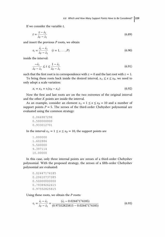
If we consider the variable t,

t � z � λ1λP � λ1

(6.89)

and insert the previous P roots, we obtain

τi � λi � λ1λP � λ1

i � 1; . . . ;P� � (6.90)

inside the interval:

�λ1λP � λ1

� t � 1 � λ1λP � λ1

(6.91)

such that the first root is in correspondence with z � 0 and the last root with z � 1.To bring these roots back inside the desired interval, xA � x � xB, we need to

only adopt a scale variation:

xi � xA � τi xB � xA� � (6.92)

Now the first and last roots are on the two extremes of the original intervaland the other K points are inside the interval.As an example, consider an element xA � 1 � x � xB � 10 and a number of

support points P � 5. The zeroes of the third-order Chebyshev polynomial areevaluated using the common strategy:

0.0669872980.5000000000.933012701

In the interval xA � 1 � x � xB � 10, the support points are

1.0000001.6028865.5000009.39711410.00000

In this case, only three internal points are zeroes of a third-order Chebyshevpolynomial. With the proposed strategy, the zeroes of a fifth-order Chebyshevpolynomial are evaluated:

0.024471741850.206107373850.500000000000.793892626150.97552825815

Using these roots, we obtain the P roots:

τi � λi � λ1λP � λ1

� �λi � 0:02447174185��0:97552825815 � 0:02447174185� (6.93)


that are

0.0000000000000000.1909830056250530.5000000000000000.8090169943749471.000000000000000

In this case, the five points are the five roots of the fifth-order Chebyshev poly-nomial inside the interval:

-0.0257311121191336 � z � 1.02573111211913

In the interval xA � 1 � x � xB � 10, the support points become

1.000000002.718847055.500000008.2811529510.0000000

which are the five roots of the fifth-order Chebyshev polynomial inside theinterval:

7.684200e-001 � x � 1.023158e+001

This selection of support points minimizes the maximum error of the polyno-mial approximation in the selected interval of a generic function when theextreme points are, in turn, support points.

In other words, whereas the five support points obtained using the roots of theChebyshev polynomial minimize the maximum absolute value of the polynomialerror function:

x � x1� � x � x2� � x � x3� � x � x4� � x � x5� �with x1, x2, x3, x4, and x5 within the interval 0; 1� �, the three support pointsobtained with the previous criterion minimize the maximum absolute value ofthe polynomial error function:

x� � x � x2� � x � x3� � x � x4� � x � 1� �in the same interval when the two extremes are, in turn, support points.Let us now consider the third strategy: The adjacent elements have one

single common support point and in this point the adjacent elements havethe same first derivative. In this case also, it is possible to find the internalpoints such that the resulting polynomial (which exploits the two derivativesat the extremes in this case) minimizes the maximum polynomial error func-tion. For instance, in the case of sixth-order polynomial valid in the interval


0 � t � 1, the three internal points are obtained by searching for the mini-mum with respect to the variable z of the maximum value of the function:

p � t2 � t � 0:5 � z� � � t � 0:5� � � t � 0:5 � z� � � t � 1� �2�� For the selection of the points, the symmetry is exploited.

In the BzzMath library, the third strategy is used to build the interpolating poly-nomials of third to sixth order.

The support points for the polynomials are as follows:Order 3:

0.0000000000000001.000000000000000

Order 4:

0.0000000000000000.5000000000000001.000000000000000

Order 5:

0.0000000000000000.3372943277480240.6627056722519761.000000000000000

Order 6:

0.0000000000000000.2449598888367150.5000000000000000.7550401111632851.000000000000000

6.7Which Variables Should Be Selected as Adaptive Parameters?

For the sake of simplicity, let us still suppose we have a single differential equa-tion:

f y´´; y´; y; x� � � 0 (6.94)

that is to be integrated within the interval xA; xB� � with the boundary conditions:

x � xA;gA y´´ xA� �; y´ xA� �; y xA� �; xA� � � 0

(6.95)

x � xB;gB y´´ xB� �; y´ xB� �; y xB� �; xB� � � 0

(6.96)

6.7 Which Variables Should Be Selected as Adaptive Parameters? 231

We have seen that the most reasonable choice for the function v a; x� � thatapproximates the unknown function y x� � is a polynomial. We have also seenthat it is usually suitable to split the interval in elements. Finally, we demon-strated that to obtain the P � 1� �-order polynomials valid inside each element, Psupport points are necessary for the first and second strategies. In the case ofthird strategy, we need the value of the variables and their first derivatives at theextremes of each element and the value of the variables in a certain number ofinternal points of the element; they are 0 for a third-order polynomial, 1 forfourth-order polynomial, 2 for fifth-order polynomial, and 3 for sixth-order poly-nomial. These points should be opportunely selected.It is now mandatory to select the most convenient form of the polynomial

v a; x� �. To do so, it is useful to compare two different formulations: the Lagrangeand central standard forms (see Chapter 1 of Vol. 2, Buzzi-Ferraris and Manenti,2010b).In the Lagrange form

v �XPi�1

yiLi (6.97)

where the generic Lagrange polynomial Li is given by

Li � �x � x1��x � x2� ∙ ∙ ∙ �x � xi�1��x � xi�1� ∙ ∙ ∙ �x � xP��xi � x1��xi � x2� ∙ ∙ ∙ �xi � xi�1��xi � xi�1� ∙ ∙ ∙ �xi � xP� (6.98)

the parameters of the polynomial coincide with the values of y in the supportpoints.In the central standard form

v � a1 � a2�x � xI � � a2�x � xI �2 � ∙ ∙ ∙ � aP�x � xI�P�1 (6.99)

the parameters of the polynomial coincide with the values of the coefficients ofthe power of x � xI� �.The Lagrange form has one major advantage over the central standard formsince the parameters ai of the function v coincide with the support ordinates yi.

This is particularly important to ensure the function continuity between twoadjacent elements without any effort.Moreover, it is important when one or both the boundary conditions are of

the following type:

x � xA; y xA� � � yA (6.100)

x � xB; y xB� � � yB (6.101)

In such a case, one or both the boundary conditions can be automatically sat-isfied by the approximating function v without any computational effort.Finally, this feature is crucial in the Galerkin method, where we need to calcu-

late the integrals that require the derivatives of the function v with respect to the


various parameters. When the Lagrange form is used, these derivatives coincidewith the different Lagrange polynomials.Nevertheless, we should observe that the polynomial v a; x� � must suit the

method selected with regard to the following purposes also:

� Estimation of the first derivatives of variables y or functions in y at the sup-port points.� Estimation of the second derivatives of variables y or functions in y at thesupport points.� Estimation of variables y or functions in y at points other than supportpoints.� Estimation of the first derivatives of variables y or functions in y at pointsother than support points.� Estimation of the second derivatives of variables y or functions in y at pointsother than support points.

For example, if the selected method requires the estimation of the residual inany point other than the support points, we should calculate

R a; x� � � f v´´ a; x� �; v´ a; x� �; v a; x� �; x� � (6.102)

which requires the estimation in such a point of the second derivative, the firstderivative, and the value of v a; x� �, which are unknown in points other than thesupport points.

The Lagrange polynomial has a structure that does not allow us to calculate thefirst and second derivatives with any great ease.

Thus, the Lagrange form, even though possible a priori, results in a very heavyprocedure when the number of support points is large (larger than 3), their posi-tion is not predetermined, and we want to calculate the derivatives in a genericpoint other than the support points.

However, it is possible to use the central standard form to represent the polyno-mial without losing the Lagrange form’s advantage of having the parameterscoinciding with the support ordinates.

First of all, a standard variable t is inserted and defined so as to have 0 at thebeginning of the element, xI , and 1 at the end of it, xF :

t � x � xIxF � xI

(6.103)

The polynomial valid for a certain element becomes

Pp�1�x� � b1 � b2t � ∙ ∙ ∙ � bPtp�1 (6.104)

where the parameters b depend on the selected element since they now dependon the support ordinates yi.


By using the support abscissas of the element, it is possible to write the follow-ing matrix (Vandermonde matrix):

V �

1 t1 t21 . . . tP�11

1 t2 t22 . . . tP�12

1 . . . . . . . . . . . .

1 . . . . . . . . . . . .

1 tP t2P . . . tP�1P

��

��(6.105)

If the support points have been selected as zeroes of the P-order Chebyshevpolynomial, that matrix is common to all the elements. Otherwise, the proceduremust be repeated for each element using the appropriate matrix V for eachof them.The parameters b can be written as follows:

b � V�1y (6.106)

even though the inverse matrix is not directly calculated (Vol. I, Buzzi-Ferrarisand Manenti, 2010a).

It is never necessary to explicitly calculate the parameters b of the polynomialsof the elements. In the following formulae, they will appear in the intermediatesteps only. Conversely, the factorization of the matrix V is required.

The first derivative in a generic point xk that corresponds to a value tk of thevariable t is obtained in the following way:

dydx

��x�xk

� b2 � 2b3tk � 3b4t2k � ∙ ∙ ∙ � �P � 1�bPtP�2k

xF � xI� wTbxF � xI

� wTV�1yxF � xI

� vTyxF � xI

(6.107)

where the vector wT is

wT � 0 1 2tk 3t2k ∙ ∙ ∙ P � 1� �tP�2k

�� (6.108)

and the vector v is calculated using the factorization of the matrix V, that is thesolution of the linear system:

VTv � w (6.109)

Note that if all the elements use the same number of support points and areselected using a common criterion, the vector wT and thus the vector v are iden-tical for all the elements.

The difference from element to element lies in the vector y and the size of thejth element dj � xF � xI� �. For this reason, it is opportune to have elements ofdifferent sizes, but the same number of optimally located support points.


Similarly, it is possible to calculate the second derivative in a generic point xkthat corresponds to the value tk of the variable t:

d2ydx2

��x�xk

� 2b3 � 6b4tk � ∙ ∙ ∙ � �P � 1��P � 2�bPtP�3k

�xF � xI �2 � qTb

�xF � xI �2� qTV�1y�xF � xI �2 �

gTy

�xF � xI �2 (6.110)

where the vector qT is

qT � 0 0 2 6tk ∙ ∙ ∙ �P � 1��P � 2�tP�3k

�� (6.111)

and the vector g is also calculated using the factorization of the matrix V.

Note that in this case also, if all the elements use the same number of supportpoints and these are selected using a common criterion, the vector qT and thusthe vector g are identical for all the elements.

In the following, we will suppose we have elements of different sizes, but with aneven number of optimally located support points.

In the methods that require the estimation of the first and second derivativesin all the support points, it is useful to calculate the following two matrices Aand B. They are the same for all the elements and for all the variables of the BVP:

A �

0 1 2t1 3t21 ∙ ∙ ∙ �P � 1�tP�21

0 1 2t2 3t22 ∙ ∙ ∙ �P � 1�tP�22

0 1 2t3 3t23 ∙ ∙ ∙ �P � 1�tP�23

0 1 ∙ ∙ ∙

0 1 ∙ ∙ ∙

0 1 2tP 3t2P ∙ ∙ ∙ �P � 1�tP�2P

��

��

V�1 (6.112)

B �

0 0 2 6t1 ∙ ∙ ∙ �P � 1��P � 2�tP�310 0 2 6t2 ∙ ∙ ∙ �P � 1��P � 2�tP�320 0 2 6t3 ∙ ∙ ∙ �P � 1��P � 2�tP�330 0 2 ∙ ∙ ∙0 0 2 ∙ ∙ ∙0 0 2 6tP ∙ ∙ ∙ �P � 1��P � 2�tP�3P

��

��V�1 (6.113)

These matrices allow us to calculate the first and second derivatives in thesupport points of each element once the ordinates in the support points areknown:

y j �Ayjdj

j � 1; . . . ;E� � (6.114)

y´´j �Byjd2j

j � 1; . . . ∞;E� � (6.115)


where yj are the values of the vector y and dj are the size of the jth element,respectively.Thus, the first and second derivatives of y are easy to calculate in correspon-

dence with the abscissas of the support points, whereas the values of y areknown since they coincide with the ordinates of the support points.In some methods, it is necessary to estimate the value of y and its first and

second derivatives in M points xm with m � 1; . . . ;M other than the supportabscissas.To do so, it is useful to collect further auxiliary matrices C, D, and F.

Note that if all the elements use the same number of points, M, and are selectedwith a common criterion, the matrices C, D, and F are identical for all the ele-ments and all the variables of the BVP.

The matrices D and F are needed for the calculation of the first and secondderivatives and are obtained in a way similar to the matrices A and B by simplyreplacing the values of support abscissas tm with the new points zm:

zm � xm � xIxF � xI

(6.116)

Analogously, the estimation of y in correspondence with xm to which a valuezm corresponds in the normalized variable is

yjx�xm � b1 � b2zm � b3z2m � ∙ ∙ ∙ � bPz

P�1m � hTb � hTV�1y � sTy

(6.117)

where the vector hT is

hT � 1 zm z2m z3m ∙ ∙ ∙ zP�1m

�� (6.118)

and the vector s is calculated using the factorization of the matrix V by solvingthe linear system:

VT s � h (6.119)

If we want to estimate the values of y in M points zm, the correspondingmatrix C is

C �1 z1 z21 z31 ∙ ∙ ∙ zP�111 ∙ ∙ ∙ ∙ ∙ ∙ ∙ ∙ ∙ ∙ ∙ ∙ ∙ ∙ ∙1 zM z2M z3M ∙ ∙ ∙ zP�1M

��V�1 (6.120)

ymj � Cyj j � 1; . . . ;E� � (6.121)

where ymj are the values of the vector y at the M points of the jth element.What we said for the polynomials obtained using the second strategy is also

valid for the Hermite polynomials built using the third strategy.

Once again, it is possible to build matrices that allow us to calculate the values ofthe variables and the first and second derivatives for each value of the


independent variable x, once the values and derivatives at the extremes of eachelement and the values of variables in an assigned number of internal points ofeach element are also known.

6.8The BVP Solution Classes in the BzzMath Library

The following classes, implemented in the BzzMath library allow us to solveBVPs with the following structure:

f y´´; y´; y; x� � � 0 (6.122)

in the interval xA; xB� � with boundary conditions:

x � xA gA y´´ xA� �; y´ xA� �; y xA� �; xA� � � 0 (6.123)

x � xB gB y´´ xB� �; y´ xB� �; y xB� �; xB� � � 0 (6.124)

The system must have

� A derivative with a maximum order 2.� Boundary conditions concentrated in two points only.� Disjoined boundary conditions.

The BzzBVP class is dedicated to the solution of BVPs with the structure(6.122)–(6.124) with the above-mentioned limitations. It uses the following clas-ses just implemented for it:

BzzFiniteElementPointsForHermitePolynomialBzzPiecewiseHermitePolynomialInterpolation

but which could also be used for other purposes.

These classes allow us to solve BVPs with the structure (6.122)–(6.124), giventhe following limitations:

1) There are no discontinuities in the variables and in the first derivativesinside the interval.

2) Each equation of the system (6.122) is related to a specific variable.3) If at one extreme point a variable has no boundary conditions, it must be

possible to evaluate the residual for the related equation without anynumerical issues.

4) If a parameter is constant, it is not related to a specific equation, but isidentified as demonstrated below.

The strategy adopted in the BzzBVP class is as follows. The interval xA; xB issplit into an assigned number of elements. The polynomial order O is alsoassigned for the approximation of the variables within each element. Such anorder can vary from 3 to 6 and is constant for all the variables of the system. If a

6.8 The BVP Solution Classes in the BzzMath Library 237

constant parameter exists, it is treated in a different manner as shown in thefollowing.

By increasing the polynomial order, both the number of necessary elementsrequired to describe the variables properly and the number of support pointswhere the residuals have to be calculated decrease, while the width of the diago-nal of the nonlinear system to be solved unavoidably increases.

Depending on the problem, a particular polynomial order may prove suitable.A low order is useful when many variables are present and very little computa-tional effort is needed for the evaluation of the residuals in a point; higher ordersare preferable otherwise.The following variables are adopted to solve the BVP:

� The values of the variables at the extremes of each element.� The values of the first derivatives at the same points.� The values of the variables at the internal points of each element. They areO-3, where O is the order of the polynomial.

The criterion to calculate the value of these variables is a variant of the orthog-onal collocation method. In a generic iteration, knowing the values of these vari-ables, it is possible to build N piecewise Hermite polynomials. Using thesepolynomials, it is possible to calculate the value of the N variables and their firstand second derivatives in the internal points for each element. These internalpoints are the Gauss quadrature points and they are 2 for a third-order, 3 for thefourth-order, 4 for the fifth-order, and 5 for the sixth-order polynomials.Once these values are known, it is possible to calculate at such points the

residuals of the system that will form the nonlinear system to be zeroed(together with the boundary conditions).

Thus, three important differences exist between this and the classical orthogonalcollocation method:

� The polynomial is a Hermite polynomial that usually performs better thanother polynomials based only on support ordinates.� It is not necessary to impose an equation for each of the N variables tomatch the derivative value of two adjacent elements.� The points where the residuals are zeroed are different from the ones usedto build the polynomial.

Note that four kinds of points exist inside the interval xA; xB.

� Extreme points of each element where the value of the N variables andtheir first derivatives is calculated. These points will be selected in an adap-tive way to improve accuracy where some variables have fast variations.� Internal points of each element where the value of the N variables is calcu-lated and the position is selected to minimize the approximation errorusing a Hermite polynomial.


� Internal points of each element where the residuals are zeroed. Thesepoints are the Gauss quadrature points.� Generic points other than the types above. Note that in the previousthree bullet points it is possible to evaluate the variables, the first andthe second derivatives by using the ancillary matrices A, B, C, D, and Fvalid for each element, and each variable of the BVP. For the sameevaluations in points other than the previous bullet points, it is neces-sary to calculate the parameters of the different polynomials for eachelement and for each variable of the BVP. These points are used onlyat the end of the computations for numerical and/or graphical verifica-tion purposes.

By using the points of the Gauss quadrature as the collocation points wherethe residuals are zeroed, in spite of the points used to build the polynomials, thefollowing advantage is obtained.

Since these points are the ones used to calculate the integral of a function, if thefunction is null in each of them, the approximate integral is also null: In otherwords, this is a necessary condition to have a null integral of the residuals foreach element.

If the number of variables and equations of the BVP system is N and the num-ber of elements is E, the total amount of variables of the nonlinear system is2N � E � 1� � � N � E � O � 3� � � N � E � O � 1� � � 2N .The equations are as follows:

� The initial boundary conditions for the variables or the residual of the equa-tion if the initial boundary condition is unavailable for this variable.� The residuals evaluated in the support points of the Gauss quadrature foreach element.� The final boundary conditions for the variables or the residual of the equa-tion if the final boundary condition is unavailable for this variable.

The total amount of equations is N � E � O � 1� � � 2N .

When a constant parameter has to be estimated, the number of equations of theBVP is N , whereas the number of variables is N � 1. The constant parameter inthe BzzBVP class must be the N � 1 variable.

When a constant parameter has to be estimated, the variables of the BVP areas follows:

� The values of the true variables at the extremes of each element.� The values of their first derivatives at the same points.� The values of the constant parameter at the same points.� The values of the true variables at the internal points of each element. Theyare O-3, where O is the order of the polynomial.


In this case, if the number of equations is N and the number of elements is E,the total amount of variables of the resulting nonlinear system is2N � E � 1� � � N � E � O � 3� � � E � 1� �.The equations are as follows:

� The initial boundary conditions for the true variables or the residual of theequation if the initial boundary condition is unavailable for this variable.� The residuals evaluated in support points of the Gauss quadrature for eachelement.� An additional equation for each element to impose the invariance of theunknown parameter.� The final boundary conditions for the true variables or the residual of theequation if the final boundary condition is unavailable for this variable.

Note that to have an even number of equations and variables, the number ofconditions to be assigned to an extreme point is N � 1. It is obtained by impos-ing one more initial or final boundary conditions with respect to the requirednumber of conditions for one variable.

For example, if the second derivative is not provided for a variable in itsrelated equation, both the initial and final boundary conditions are assigned tosuch a variable.The task of an object of the BzzFiniteElementPointsForHermitePoly-

nomial class is to initialize all the vectors and matrices needed to estimate thevalues of the variables in the necessary points inside the BzzPiecewiseHermi-

tePolynomialInterpolation class.An object of the BzzFiniteElementPointsForHermitePolynomial

class can be initialized in different ways.The user can provide the extremes of the elements to split the interval. If we

indicate with BzzVector x the vector (dimensioned E � 1), the result is

BzzFiniteElementPointsForHermitePolynomial fep;fep(polynomiumOrder,x);

The user can assign some points inside the interval and the number of ele-ments for each subinterval. For instance:

BzzFiniteElementPointsForHermitePolynomial fep;int numSelectedPoints = 4;BzzVector x(numSelectedPoints,0.,0.1,0.9,1.);BzzVectorInt numInternalPoints(3,30,10,30);fep(polynomiumOrder,x,numInternalPoints);

In this case, the user provides four points: 0.,0.1,0.9,1.The interval 0.,0.1 will be split into 30 subintervals; the interval

0.1,0.9 into 10; the interval 0.9,1 into 30. This possibility allows us toeasily insert additional points where large variations are predicted for one ormore variables.


The object of this class is initialized in this way only to provide initial discreti-zation in elements. The number of elements and their position can also varyaccording to the results.The object fep has numerous functions that can be exploited inside the

BzzPiecewiseHermitePolynomialInterpolation and BzzBVP classes.The main functions are

fep.GetSupportPointsForValues(&sv);fep.GetSupportPointsForDerivatives(&sd);fep.GetSupportPoints(&s);

The values of all the points where the N variables are estimated are collectedin the object sv.The values of all the points where the related first derivatives are estimated are

collected in the object sd.The values of all the points where the residuals to be zeroed are calculated are

collected in the object s.An object of the BzzPiecewiseHermitePolynomialInterpolation

class can be initialized in two ways:

BzzPiecewiseHermitePolynomialInterpolation p1p1(fep,yy1,d1y1);

where fep is an object of the previous class, BzzVector yy1 are the values ofthe variable 1 in the points sv, and BzzVector d1y1 are the values of the firstderivative of the variable 1 in the points sd.With this initialization, the number of functions of the object p1 is limited to

those strictly required to calculate the residuals in the points s obtained by theobject fep.

p1.GetValueInSupportPoints(fep, &sy1);p1.GetFirstDerivativeInSupportPoints(fep, &sd1y1);p1.GetSecondDerivativeInSupportPoints(fep, &sd2y1);

The values of the variable 1 and its first and second derivatives at the supportpoints s are collected in BzzVector sy1, BzzVector sd1y1, BzzVector

sd2y1. With these values known, it is very simple to write the equations of theresiduals for this kind of variable.

Clearly, if a variable or its first or second derivative does not appear in any equa-tion, the corresponding function does not have to be used.

If the object of the BzzPiecewiseHermitePolynomialInterpolation

class is initialized as follows:

BzzPiecewiseHermitePolynomialInterpolation p1p1(fep,yy1,d1y1,1);


it is possible to use other functions also. The most important of these are

double y1 = p1(fep,z);double d1 = p1(fep,z,1);double d2 = p1(fep,z,2);

y1 contains the value of the variable 1 at the generic point z estimated usingthe piecewise Hermite polynomial. d1 contains the value of the first derivative ofthe variable 1 at the generic point z. d2 contains the value of the second deriva-tive of the variable 1 at the generic point z. An object of each of the two classestogether with an object of the BzzNonLinearSystemSparse class allows tosolve a BVP.

Example 6.1

Solve the following BVP:

y´´ � �10000yusing the boundary conditions:

xA � 0; y xA� � � 1

xB � 1; y xB� � � cos 100� � � sin 100� �The analytical solution for this problem is

y � cos 100x� �The program is

#define BZZ_COMPILER 0#include “BzzMath.hpp”void BvpExample1_1(BzzVector &x,BzzVector &f);int numElements;int numExteriorPoints;int polynomiumOrder; // 3, 4, 5, 6int numSupportPointsForValues;int numSupportPointsForDerivatives;int numSupportPoints;int numSupportPointsInEachElement;int numConnectionPoints;int numVariablesNLS;

BzzFiniteElementPointsForHermitePolynomial fep;BzzPiecewiseHermitePolynomialInterpolation p1;BzzVector sv,s;BzzVector yy1,d1y1,d2y1;BzzVector sy1,sd1y1,sd2y1;main(void)

{


// y”+lamda2*y =0int i,j,k,l;lambda = 100.;lambda2 = lambda * lambda;numExteriorPoints = 55;polynomiumOrder = 4;double dx;BzzVector x(numExteriorPoints);dx = 1. / double(numExteriorPoints - 1);x[1] = 0.;for(i = 2;i <= numExteriorPoints - 1;i++)

{x[i] = x[i - 1] + dx;}

x[numExteriorPoints] = 1.;fep(polynomiumOrder,x);fep.GetSupportPointsForValues(&sv);fep.GetSupportPoints(&s);numSupportPointsForValues =

fep.GetNumSupportPointsForValues();numSupportPointsForDerivatives =

fep.GetNumSupportPointsForDerivatives();numSupportPoints = s.Size();numVariablesNLS = numSupportPointsForValues

+ numSupportPointsForDerivatives;

ChangeDimensions(numSupportPointsForValues, &yy1);ChangeDimensions(numSupportPointsForDerivatives,

&d1y1);BzzVector y0(numVariablesNLS);BzzNonLinearSystemSparse nls(y0,

BvpExample1_1,polynomiumOrder,polynomiumOrder);

nls();nls.BzzPrint(“Results”);

BzzVector y,f;nls.GetSolution(&y, &f);

j = 1;k = 1;for(i=1;i < numSupportPointsForDerivatives;i++)

{yy1[k++] = y[j++];d1y1[i] = y[j++];for(l = 1;l <= polynomiumOrder - 3;l++)


yy1[k++] = y[j++];}

yy1[k++] = y[j++];d1y1[numSupportPointsForDerivatives] = y[j++];

p1(fep,yy1,d1y1,1);int nnxx;nnxx = 600;BzzVector xx(nnxx);BzzMatrix YY(2,nnxx);xx[1] = sv[1];xx[nnxx] = sv[numSupportPointsForValues];YY(1,1) = yy1[1];YY(2,1) = 1.; // analyticalYY(1,nnxx) = yy1[numSupportPointsForValues];YY(2,nnxx) = cos(lambda) + sin(lambda);

for(i = 2; i < nnxx;i++){xx[i] = xx[i - 1] + 1. / double(nnxx - 1);YY(1,i) = p1(fep,xx[i]);YY(2,i) = cos(lambda * xx[i]) +

sin(lambda * xx[i]);}

BzzSave save(“PlotY.mtr”);save << xx << YY;save.End();}

void BvpExample1_1(BzzVector &y,BzzVector &f){int i,l;int j = 1;int k = 1;for(i=1;i < numSupportPointsForDerivatives;i++)

{yy1[k++] = y[j++];d1y1[i] = y[j++];for(l = 1;l <= polynomiumOrder - 3;l++)

yy1[k++] = y[j++];}

yy1[k++] = y[j++];d1y1[numSupportPointsForDerivatives] = y[j];p1(fep,yy1,d1y1);p1.GetValueInSupportPoints(fep, &sy1);p1.GetSecondDerivativeInSupportPoints(fep,


&sd2y1);f[1] = yy1[1] - 1.;j = 2;for(i = 1;i <= numSupportPoints; i++)

f[j++] = sd2y1[i] + lambda2 * sy1[i];f[j] = yy1[numSupportPointsForValues] –

cos(lambda) - sin(lambda);}

The results are reported in Figure 6.6.The numerical solution (solid line) is overlapped with the analytical solution

(dots). To make use of the classes easier, their objects have been inserted into aclass BzzBVP, implemented solely to solve BVP with the structure (6.122)–(6.124).Note that by using the following statement:

BzzVector y0(numVariablesNLS);

for the initial values of the nonlinear system variables, all of them are zero at thebeginning.The BzzBVP class has only one constructor (default constructor):

BzzBVP bvp;

The object bvp is initialized as follows:

bvp(numEquations,numVariables,equationValuePresence,equationFirstDerivativePresence,equationSecondDerivativePresence,leftBoundarySecondDerivativePresence,

Figure 6.6 Solution of the BVP.


rightBoundarySecondDerivativePresence,ResidualsName,LeftBoundaryName,RightBoundaryName,criticalParametersSoft,criticalParametersRequired,x,Y,numInternalPoints,initialFinal);

The number of equations is assigned at the integer variable:

int numEquations

The number of variables is assigned at the integer variable:

int numVariables

If it is different from the number of equations, it means that one or more var-iables are constant parameters.

In the BzzBVP class, only the case with one single constant parameter is consid-ered. Moreover, the constant parameter must be the N � 1 variable.

Other elements are

BzzVectorInt equationValuePresence(numVariables)

If the ith variable yi is explicitly present in certain equations (6.122), it is nec-essary to evaluate its value. If so, the corresponding element of the vector equa-

tionValuePresence is equal to 1; it is 0 if the variable does not appearanywhere in the equations.

BzzVectorInt equationFirstDerivativePresence(numVariables)

If the ith first derivative yi is explicitly present in certain equations (6.122), it isnecessary to evaluate its value. If so, the corresponding element of the vectorequationFirstDerivativePresence is equal to 1; it is 0 if it does notappear anywhere in the equations or if it is constant.

BzzVectorInt equationSecondDerivativePresence(numVariables)

If the ith second derivative y´´i is explicitly present in certain equations (6.122),it is necessary to evaluate its value. If so, the corresponding element of the vectorequationSecondDerivativePresence is equal to 1; it is 0 if it does notappear anywhere in the equations or if it is constant.

BzzVectorInt leftBoundarySecondDerivativePresence(numVariables)

BzzVectorInt rightBoundarySecondDerivativePresence(numVariables)


If the second derivative of the variable is present as a variable in left or in theright boundary conditions, it is necessary to know its value. If so, the corre-sponding element of the vector is equal to 1; it is 0 if it does not appear any-where in Equations 6.123 and 6.124, respectively.Then, the name of the function where the equation residuals are calculated is

given:

ResidualsName

The prototype is

void ResidualsName(double x, BzzVector &y,BzzVector &d1, BzzVector &d2,BzzVector &criticalParameters,BzzVector &r);

In this function, the residuals r of the equations must be evaluated, given

� x (value of the point where the residuals have to be evaluated);� y (value of the variables in x);� d1 (values of the first derivatives of the variables in x);� d2 (values of the second derivatives of the variables in x).

criticalParameters is the value of the critical parameters used during thecurrent iteration.The vectors y, d1, and d2 are sized numVariables, whereas the vector r is

sized numEquations.The name of the function where the residuals are calculated at the initial

point is

LeftBoundaryName

The prototype is

void LeftBoundaryName(double x, BzzVector &y,BzzVector &d1, BzzVector &d2,BzzVector &criticalParameters,BzzVector &r,double *r1);

In the vector r, the value of the residual of the initial boundary condition, ifany, is returned; otherwise, the residual of the equation is calculated.

The last double in the argument is useful only when a constant parameter ispresent. In this case, the value of the residual of the equation with overabundantboundary conditions has to be provided at an extreme point. The user mustselect between the two alternatives: providing such a residual at either the initialor the final bound.


The name of the function where the residuals are calculated at the finalpoint is

RightBoundaryName

Its prototype is the same as the one of the previous function. In the vector r,

the value of the residual of the final boundary condition, if any, is returned; theresidual of the equation is calculated otherwise. The double has the same aimas the double of the previous function LeftBoundaryName and works asalternative to it.

BzzVector criticalParametersSoftBzzVector criticalParametersRequired

There could be some parameters in the equations, criticalParame-

tersRequired, which might have some values that make solving theBVP hard. In this case, it is useful to also provide a value for them,criticalParametersSoft, thereby making the problem easier to solve.The object bvp self-modify such a vector starting from the proposedvalue, criticalParametersSoft, up to the required parameters, whenpossible.In the matrix

BzzMatrix Y(numVariables,numPoints);

we provide the first guesses of the variables in correspondence with some pointsgiven in the vector:

BzzVector x(numPoints);

Note that the x[1] must be the initial point and x[numPoints] the finalone.The variable x splits the interval in numPoints - 1 subintervals. They in turn

are split into a number of elements. For instance, if numPoints is 3,

BzzVectorInt numInternalPoints(numPoints-1,5,30);

The first subinterval is split into 5 elements, the second into 30 elements.

int initialFinal;

When a constant parameter requires estimation, it is necessary to providean initial or a final additional condition. The variable initialFinal isrequired to communicate to the object of the BzzBVP class, which of thetwo possibilities has been selected by the user: If the additional condition isthe initial one, the value of this variable is 0; it is 1 otherwise (final condi-tion). The value of this variable is pointless when no constant parametersneed estimation.


Example 6.2

Solve the problem in the previous example using an object from the BzzBVP

class. The program is

#define BZZ_COMPILER 0#include “BzzMath.hpp”void Residuals2(double x, BzzVector &y,

BzzVector &d1, BzzVector &d2, BzzVector &cP,BzzVector &r);

void LeftBoundary2(double x, BzzVector &y,BzzVector &d1, BzzVector &d2, BzzVector &cP,BzzVector &r,double *r1);

void RightBoundary2(double x, BzzVector &y,BzzVector &d1, BzzVector &d2, BzzVector &cP,BzzVector &r,double *r1);

void main(void){int numEquations = 1;int numVariables = 1;BzzVectorInt eqValuePresence(numVariables,1);BzzVectorInt eqFirstDerivativePresence

(numVariables,0);BzzVectorInt eqSecondDerivativePresence

(numVariables,1);BzzVectorInt leftSecondDerivativePresence

(numVariables,0);BzzVectorInt rightSecondDerivativePresence

(numVariables,0);BzzVector criticalParametersSoft;BzzVector criticalParametersRequired;BzzVector x(2,0.,1.);BzzMatrix Y(numVariables,2);BzzVectorInt numInternalPoints(1,50);int initFinal;BzzBVP bvp;bvp(numEquations,numVariables,equValuePresence,eqFirstDerivativePresence,eqSecondDerivativePresence,Residuals2,LeftBoundary2,RightBoundary2,criticalParametersSoft,criticalParametersRequired,x,Y,numInternalPoints,initFinal);bvp();bvp.BzzPrint(“Results”);}


void Residuals2(double x,BzzVector &y,BzzVector &d1,BzzVector &d2,BzzVector &cP,BzzVector &r)

{r[1] = d2[1] + 100000. * y[1];}

void LeftBoundary2(double x,BzzVector &y,BzzVector &d1,BzzVector &d2,BzzVector &cP,BzzVector &r,double *r1)

{r[1] = y[1] - 1.;}

void RightBoundary2(double x,BzzVector &y,BzzVector &d1, BzzVector &d2, BzzVector &cP,BzzVector &r,double *r1)

{r[1] = y[1] – cos(100.) - sin(100.);}

An object from the BzzBVP class automatically selects the order of the poly-nomial. It is possible to ask for a polynomial with the order between 3 and 6 bymeans of the function SetPolynomiumOrder. For example, to select a fifth-order polynomial, we use

bvp.SetPolynomiumOrder(5);

The control of the error is carried out by calculating the residuals in differentpoints other than the support points adopted to zero the residuals. The defaultvalue is 10�6 for the absolute error of all residuals. It is possible to vary this valueusing the function SetAbsTolerance.An object of the BzzBVP class checks whether the solution is achieved in the

following manner.The first necessary (but not sufficient) condition to identify the achievement of

the solution is based on the maximum value of the residuals at the supportpoints after the solution of the nonlinear system. If such a value is too large(meaning that no solution is found for the nonlinear system), the number of ele-ments is increased and the order of the polynomial is often increased as well.The selection of the new points does not use the solution achieved since it isunreliable.If, on the other hand, the nonlinear system is solved satisfactorily, the residuals

are checked at the points shared between adjacent elements. If the residuals arevery satisfactory, the problem is considered solved, unless the critical parameteris not yet at its nominal value. This problem will be tackled in the next section. Ifthe residuals are not satisfactory enough in certain element connection points,the number of elements and the order of the polynomial are increased. Theselection of new points to increase the number of elements is based on the resid-ual error: the larger the error, the larger the number of points inserted in its


neighborhood. Note that in this case also, the solution is not exploited for meshpoint selection. Finally, if the residuals are almost satisfactory in some connec-tion points, but it may be possible to improve the solution in any case, the strat-egy proposed in the next section is adopted.

6.9Adaptive Mesh Selection

In many BVPs, it is convenient to use elements of different dimensions to suitthe local difficulties of the problem. Different strategies to improve the selectionof the subsequent iterations have been proposed based on the results obtainedwith an assigned distribution of initial points. For a comprehensive investigationof this, we refer readers to Russell and Christiansen (1978).

In the BzzBVP class, the following strategy is adopted. It is applied only whenthe errors of the residuals are practically zero at the support points and are rea-sonably small (but still unsatisfactory) at the connection points. It is also adoptedwhen there is a critical parameter and we want to exploit the solution achievedusing a softer value of that parameter.

Once the calculation is carried out with an assigned selection of mesh points,the piecewise Hermite polynomials of each variable are used to obtain a detaileddescription of their first derivative in the interval xA; xB. It is thus possible toobtain a diagram where the abscissas are the values of the variable x with a con-stant interval, whereas the ordinate is the maximum absolute value of the firstderivative of all the variables added to the value obtained in the previous interval.This produces a monotone trend that originates from 0.Now let us consider the same diagram with the ordinates and abscissas

swapped. If we assign the number of new elements that we want to take intoconsideration and analyze the abscissas with a constant step, equal to the onerelated to the number of selected elements, the number of new ordinates is auto-matically improved where the derivatives are large (in absolute value) andreduced where the derivatives are small.For example, the problem in Example 6.6 solved with a certain selection of

elements leads to the plot in Figure 6.7.The function varies significantly in the interval 0–0.33, but is quite constant in

the interval 0.5–1. The plot of the cumulated derivatives with respect to the nor-mal abscissas is reported in Figure 6.8. The plot obtained by swapping ordinatesand abscissas is in Figure 6.9.By splitting the interval 0–5.02 into a predetermined number of even-sized

elements, we obtain denser ordinate values where the curve is more smooth andsparser ones where the curve is stiff. For example, by using 20 elements, weobtain the following points and elements:

1 1.061e-0012 1.105e-001 4.378e-003

6.9 Adaptive Mesh Selection 251

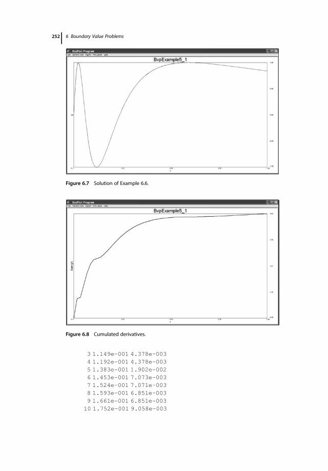
3 1.149e-001 4.378e-0034 1.192e-001 4.378e-0035 1.383e-001 1.902e-0026 1.453e-001 7.073e-0037 1.524e-001 7.071e-0038 1.593e-001 6.851e-0039 1.661e-001 6.851e-003

10 1.752e-001 9.058e-003

Figure 6.7 Solution of Example 6.6.

Figure 6.8 Cumulated derivatives.


11 1.866e-001 1.141e-00212 2.256e-001 3.904e-00213 2.561e-001 3.045e-00214 2.793e-001 2.320e-00215 3.028e-001 2.349e-00216 3.292e-001 2.649e-00217 3.617e-001 3.245e-00218 4.068e-001 4.515e-00219 4.915e-001 8.466e-00220 1.000e+000 5.085e-001

Note that they are denser where the original curve varies significantly.

6.10Case studies

In this section, we look at the BVPs proposed by different authors.

The programs relating to the following case studies can be found in the directoryVol4_Chapter6 in the WileyVol4.zip file available at the following web site:http://www.chem.polimi.it/homes/gbuzzi.

Example 6.3

Solve the following BVP:

1 � x� � y´´ � xy´ � y � 0

Figure 6.9 Swapped ordinates–abscissas plot.

6.10 Case studies 253


with the boundary conditions:

xA � 0; y xA� � � exp 0� �xB � 3; y xB� � � 3 � exp 3� �

This problem does not present any difficulty, but it has the advantage of hav-ing an analytical solution, which might suit as test of the numerical solution. Theanalytical solution for this problem is

y � x � exp x� �The plot of the achieved solution is overlapped with that of the analytical solu-

tion (Figure 6.10).

Example 6.4

Solve the following BVP proposed by Russell and Christiansen (1978):

y´´ � 2γ xy´ � y� � � 0


xA � 0; y xA� � � 1

xB � 1; y xB� � � exp �γ� �This problem does not present any difficulty when γ is relatively small. The

critical value proposed by the authors for a hard test of BVP programs is

Figure 6.10 BVP solution for Example 6.3.


γ � 150. Integrate the system using the proposed parameter and γ � 3000. Inthis case too, the analytical solution is known:

y � exp �γx2� �The solution obtained for γ � 3000 is overlapped with the analytical solution

(Figure 6.11).

Example 6.5


εy´´ � 2 � x2� �

y � 1 � 0


xA � 0; y xA� � � 0:5

xB � 1; y xB� � � 0

This problem does not present any difficulty when ε is relatively large. Thecritical value proposed by the authors for a hard test of BVP programs isε � 10�4. Integrate the system using the proposed parameter and ε � 10�5. Inthis case too, the analytical solution is known:

y � 12 � x2

� exp � 1 � xffiffiffiε

p !

� exp � 1 � xffiffiffiε

p !

Figure 6.11 BVP solution for the Example 6.4.


The solution obtained for ε � 10�5 is overlapped with the analytical solution(Figure 6.12).

Example 6.6


y´´ � 2xy´ � 1

x4y � 0


xA � 13π

; y xA� � � 0

xB � 1; y xB� � � sin 1� �This problem has an oscillating solution. In this case also, we know the analyt-

ical solution:

y � sin1x

� �

The numerical and analytical solutions are overlapped (Figure 6.7).



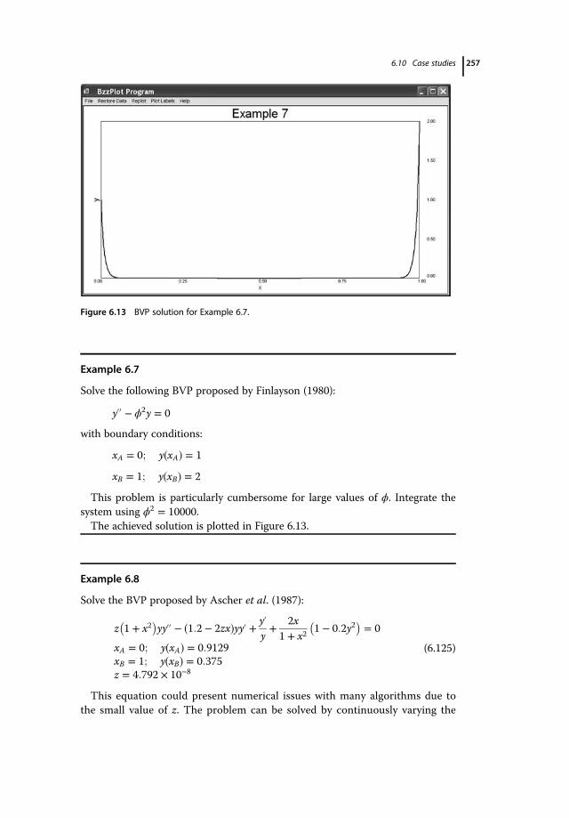
Example 6.7

Solve the following BVP proposed by Finlayson (1980):

y´´ � ϕ2y � 0

with boundary conditions:

xA � 0; y xA� � � 1

xB � 1; y xB� � � 2

This problem is particularly cumbersome for large values of ϕ. Integrate thesystem using ϕ2 � 10000.The achieved solution is plotted in Figure 6.13.

Example 6.8

Solve the BVP proposed by Ascher et al. (1987):

z 1 � x2� �

yy´´ � 1:2 � 2zx� �yy´ � y´y� 2x1 � x2

1 � 0:2y2� � � 0

xA � 0; y xA� � � 0:9129xB � 1; y xB� � � 0:375z � 4:792 � 10�8

(6.125)

This equation could present numerical issues with many algorithms due tothe small value of z. The problem can be solved by continuously varying the



parameter z, for instance, from 10�2 to the desired value (Figures 6.14 and6.15).Once the solution for this value is easily achieved even when starting from

arbitrary mesh points, the solution itself is used to improve the selection of themesh points by means of the technique described in Section 6.9.

Figure 6.14 BVP solution for Example 6.8 with z � 10�2.

Figure 6.15 BVP solution for Example 6.8 with z � 2:5 � 10�3.


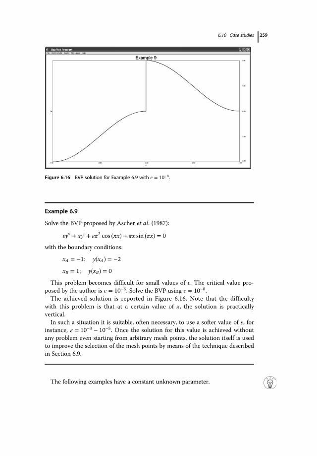
Example 6.9

Solve the BVP proposed by Ascher et al. (1987):

εy´´ � xy´ � επ2 cos πx� � � πx sin πx� � � 0


xA � �1; y xA� � � �2xB � 1; y xB� � � 0

This problem becomes difficult for small values of ε. The critical value pro-posed by the author is ε � 10�6. Solve the BVP using ε � 10�8.The achieved solution is reported in Figure 6.16. Note that the difficulty

with this problem is that at a certain value of x, the solution is practicallyvertical.In such a situation it is suitable, often necessary, to use a softer value of ε, for

instance, ε � 10�3 � 10�5. Once the solution for this value is achieved withoutany problem even starting from arbitrary mesh points, the solution itself is usedto improve the selection of the mesh points by means of the technique describedin Section 6.9.

The following examples have a constant unknown parameter.

Figure 6.16 BVP solution for Example 6.9 with ε � 10�8.


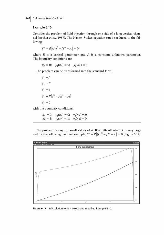
Example 6.10

Consider the problem of fluid injection through one side of a long vertical chan-nel (Ascher et al., 1987). The Navier–Stokes equation can be reduced to the fol-lowing:

f ´´´ � R f ´� �2 � f f ´´ � A� � � 0

where R is a critical parameter and A is a constant unknown parameter.The boundary conditions are

xA � 0; y1 xA� � � 0; y2 xA� � � 0

The problem can be transformed into the standard form:

y1 � f

y2 � f ´

y1 � y2

y´2 � R y22 � y1y2 � y3� �

y3 � 0


xA � 0; y1�xA� � 0; y2�xA� � 0xB � 1; y1�xB� � 1; y2�xB� � 0

The problem is easy for small values of R. It is difficult when R is very largeand for the following modified example: f ´´´ � R f ´� �2 � f f ´ � A

� � � 0 (Figure 6.17).

Figure 6.17 BVP solution for R = 10,000 and modified Example 6.10.


Example 6.11

This example too comes from Ascher et al. (1987):

y´´ � 1 � y´� �2� �1:5B � y � 2λ� � � y´ 1 � y´� �2� �

x� 0

xA � 0; y xA� � � 0; y´ xA� � � 0xB � 1; y´ xB� � � cot ϑ� �

where B � 10 is a constant parameter. λ is a constant unknown parameter. Theproblem is relatively easy when ϑ is not too small. The difficulty increases whenϑ ! 0. Solve the problem with ϑ � 10�20 (Figure 6.18).

Example 6.12

The problem of swirling flows leads to the solution of Navier–Stokes equations,which often involve a dimension reduction and are obtained numerically (Grcar,1996). By assuming that the flow has rigid rotational symmetry, axial velocityand temperature independent of the radius, density independent of the pressurevariation, and pressure quadratic with respect to the radius and independent ofthe axial profile, the general model is

ddx

μ�T � dFdx

��Hρ�T � dF

dx� ρ�T ��G2 � F2� � λ � 0



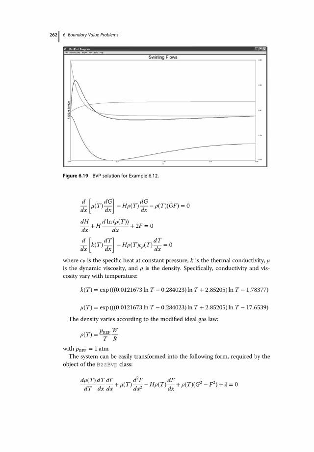
ddx

μ�T � dGdx

��Hρ�T � dG

dx� ρ�T ��GF� � 0

dHdx

�Hd ln �ρ�T ��

dx� 2F � 0

ddx

k�T � dTdx

��Hρ�T �cp�T � dTdx � 0

where cP is the specific heat at constant pressure, k is the thermal conductivity, μis the dynamic viscosity, and ρ is the density. Specifically, conductivity and vis-cosity vary with temperature:

k T� � � exp 0:0121673 ln T � 0:284023� � ln T � 2:85205� � ln T � 1:78377� �

μ T� � � exp 0:0121673 ln T � 0:284023� � ln T � 2:85205� � ln T � 17:6539� �The density varies according to the modified ideal gas law:

ρ T� � � pREFT

WR

with pREF � 1 atmThe system can be easily transformed into the following form, required by the

object of the BzzBvp class:

dμ�T �dT

dTdx

dFdx

� μ�T � d2F

dx2�Hρ�T � dF

dx� ρ�T ��G2 � F2� � λ � 0



dμ�T �dT

dTdx

dGdx

� μ�T �d2Gdx2

�Hρ�T �dGdx

� ρ�T ��GF� � 0

dHdx

�H1

ρ�T �d ρ�T� �dT

dTdx

� 2F � 0

dk�T �dT

dTdx

� �2

� k�T � d2Tdx2

�Hρ�T �cP T� � dTdx

� 0

The numerical solution of F, G, H, and T for the equations, boundary condi-tions, and fluid properties given above is reported in Figure 6.19.


References

Aiken, R.C. and Lapidus, L. (1974) An effectivenumerical integration method for typicalstiff systems. AIChE J., 20 (2), 368–375.

ANSYS (2009) ANSYS FLUENT 12.0: UDFManual.

Ascher, U.R., Mattheij, R.M.M., and Russell,R.D. (1987) Numerical Solution ofBoundary Value Problems for OrdinaryDifferential Equations, Society forIndustrial and Applied Mathematics.

Ascher, U.M. and Petzold, L.R. (1998)Computer Methods for OrdinaryDifferential Equations and Differential–Algebraic Equations, SIAM: Society forIndustrial and Applied Mathematics.

Atkinson, K.E. (1989) An Introduction toNumerical Analysis, John Wiley & Sons,Inc., New York.

Bowen, J.R., Acrivos, A., and Oppenheim, A.K.(1963) Singular perturbation refinement toquasi-steady state approximation inchemical kinetics. Chem. Eng. Sci., 17 (3),177–188.

Buchanan, J.L. and Turner, P.R. (1992)Numerical Methods and Analysis,McGraw-Hill, New York.

Burnett, D.S. (1987) Finite Element Analysis:From Concepts to Applications, AddisonWesley Publishing Company.

Buzzi-Ferraris, G. (1994) Scientific C++:Building Numerical Libraries, the Object-Oriented Way, 2nd ed., Addison-Wesley,Cambridge University Press.

Buzzi-Ferraris, G. and Manenti, F. (2010a)Fundamentals and Linear Algebra for theChemical Engineer: Solving NumericalProblems, Wiley-VCH Verlag GmbH,Weinheim, Germany.

Buzzi-Ferraris, G. and Manenti, F. (2010b)Interpolation and Regression Models forthe Chemical Engineer: Solving NumericalProblems, Wiley-VCH Verlag GmbH,Weinheim, Germany.

Buzzi-Ferraris, G. and Manenti, F. (2011a)Data Interpretation and Correlation. Kirk-Othmer Encyclopedia of ChemicalTechnology, 5th edn, John Wiley & Sons,Inc., New York.

Buzzi-Ferraris, G. and Manenti, F. (2011b)Outlier detection in large-scale data sets.Comput. Chem. Eng., 35, 388–390.

Buzzi-Ferraris, G. and Manenti, F. (2012)Improving the selection of interior pointsfor one-dimensional finite elementmethods. Comput. Chem. Eng., 40, 41–44.

Buzzi-Ferraris, G. and Manenti, F. (2014)Nonlinear Systems and Optimization forthe Chemical Engineer: Solving NumericalProblems, Wiley-VCH Verlag GmbH,Weinheim, Germany.

Buzzi-Ferraris, G. and Tronconi, E. (1993) Animproved convergence criterion in thesolution of nonlinear algebraic equations.Comput. Chem. Eng., 17, 419.

Byrne, G.D. and Hindmarsh, A.C. (1987) Stiffode solvers: a review of current and comingattractions. J. Comput. Phys., 70, 1–62.

Calderbank, P.H. (1953) Contact-processconverter design. Chem. Eng. Prog., 49, 585.

Carias-Henriquez, A., Pietrzyk, S., andDujardin, C. (2013) Modelling andoptimization of IR cell devoted to in situand operando characterization of catalysts.Catal. Today, 205, 134–140.

Centi, G., Ciambelli, P., Perathoner, S., andRusso, P. (2002) Environmental catalysis:

265


trends and outlook. Catal. Today, 75,3–15.

Chan, Y.N.I., Birnbaum, I., and Lapidus, L.(1978) Solution of stiff differentialequations and the use of imbeddingtechniques. Ind. Eng. Chem. Fund., 17 (3),133–148.

Corbetta, M., Manenti, F., and Visconti, C.G.(2014) CATalytic – Post-Processing(CAT-PP): a new methodology for theCFD-based simulation of highly dilutedreactive heterogeneous systems. Comput.Chem. Eng., 60, 76–85.

Curtis, A.R., Powell, M.J.D., and Reid, J.K.(1974) On the estimation of sparseJacobian matrices. J. Inst. Math. Appl., 13,117–119.

Cutler, C.R. and Ramaker, B.L. (1980)Dynamic matrix control: a computercontrol algorithm. Proceedings of the JointAutomatic Control Conference.

Dahlquist, G. (1963) A special stabilityproblem for linear multistep methods. BITNumer. Math., 3, 27–43.

Deutschmann, O. (2001) Interactions betweentransport and chemistry in catalyticreactors. Unpublished Habilitation thesis,Ruprecht-Karls-University of Heidelberg.

Dones, I., Manenti, F., Preisig, H.A., andBuzzi-Ferraris, G. (2010) Nonlinear modelpredictive control: a self-adaptiveapproach. Ind. Eng. Chem. Res., 49,4782–4791.

Dones, I., Preisig, H.A., and de Graaf, S.(2009) Towards the dynamic initialisationof C4 splitter models, in Proceedings of the1st Annual Gas Processing Symposium,Qatar (eds H. Alfadala, G.V. Rex Reklaitis,and M.M. El-Halwagi), Elsevier, p. 1.

Edgar, T.F. and Himmelblau, D.M. (2001)Optimization of Chemical Processes, 2ndedn, McGraw-Hill Publishing Co.

European Parliament (2007) Regulation (EC)No. 715/2007 of the European Parliamentand of the Council of 20 June 2007on typeapproval of motor vehicles with respect toemissions from light passenger andcommercial vehicles (Euro 5 and Euro 6)and on access to vehicle repair andmaintenance information.

Field, R.J. and Noyes, R.M. (1974) Oscillationsin chemical systems: IV. Limit cyclebehavior in a model of a real chemical

reaction. J. Chem. Phys., 60,1877–1884.

Finlayson, B.A. (1980) Nonlinear Analysis inChemical Engineering, ChemicalEngineering Series, McGraw-Hill.

Gear, C.W. (1971) Numerical Initial ValueProblems in Ordinary Differential Equations,Prentice-Hall, Englewood Cliffs, NJ.

Gottwald, B.A. (1977) MISS – ein einfachessimulations: system fur biologische undchemische Prozesse. EDV Medizin Biol.,3, 85–90.

Grcar, J.F. (1996) The Twopnt Program forBoundary Value Problems, SAND91-8230,Livermore (CA), USA.

Hairer, E. and Wanner, G. (2010) SolvingOrdinary Differential Equations II,Springer, Berlin, Germany.

Hindmarsh, A.C. (1983) ODEPACK, asystematized collection of ODE solvers, inScientific Computing (ed. R.S. Stepleman),North-Holland, Amsterdam, pp. 55–64.

Kahaner, D., Moler, C., and Nash, S. (1989)Numerical Methods and Software,Prentice-Hall, Englewood Cliffs, NJ.

Lapidus, L. and Seinfeld, J.H. (1971)Numerical Solution of OrdinaryDifferential Equations, Volume 74 ofMathematics in Science and Engineering,Academic Press.

Lee, K.Y. and Aris, R. (1963) Optimaladiabatic bed reactors for sulfur dioxidewith cold shot cooling. Ind. Eng. Chem.Process Des. Dev., 2 (4), 300–306.

Luyben, W.L. (1996) Process Modeling,Simulation and Control for ChemicalEngineers, 2nd edn, Chemical EngineeringSeries, McGraw-Hill.

Kolaczkowski, S.T., Chao, R., Awdry, S., andSmith, A. (2007) Application of a CFDcode (FLUENT) to formulate models ofcatalytic gas phase reactions in porouscatalyst pellets. Chem. Eng. Res. Des., 85,1539–1552.

Krishnamurthy, R. and Taylor, R. (1985a)Nonequilibrium stage model ofmulticomponent separation processes.AIChE J., 31, 1973–1985.

Krishnamurthy, R. and Taylor, R. (1985b) Anonequilibrium stage model ofmulticomponent separation processes.Part I: model description and method ofsolution. AIChE J., 31, 449–456.

266 References

Løvfall, B.T. (2008) Computer realisation ofthermodynamic models using algebraicobjects. PhD thesis, NTNU, Trondheim,Norway.

Malengé, J.P. and Villermaux, J. (1967)Simulation of heat-transfer phenomena ina Rotary Kiln. Industrial & EngineeringChemistry Process Des. Dev., 6 (4),535.

Manenti, F. (2011) Considerations onnonlinear model predictive controltechniques. Comput. Chem. Eng., 35,2491–2509.

Manenti, F., Dones, I., Buzzi-Ferraris, G., andPreisig, H.A. (2009) Efficient numericalsolver for partially structured differentialand algebraic equation systems. Ind. Eng.Chem. Res., 48, 9979–9984.

Meunier, F.C. (2010) The design and testingof kinetically appropriate operandospectroscopic cells for investigatingheterogeneous catalytic reactions. Chem.Soc. Rev., 39, 4602–4614.

Morari, M. and Lee, J.H. (1999) Modelpredictive control: past, present andfuture. Comput. Chem. Eng., 23,667–682.

Naphtali, L.M. and Sandholrn, D.P. (1971)Multicomponent separation calculationsby linearization. AIChE J., 17, 148.

Rice, R.J. (1993) Numerical Methods,Software, and Analysis, Academic Press,London.

Robertson, H.H. (1967) Solution of a seat ofreaction rate equations, in NumericalAnalysis (ed. J. Walsh), Thomson BookCo., Washington DC.

Russell, R.D. and Christiansen, J. (1978)Adaptive mesh selection strategies forsolving boundary value problems. SIAM J.Numer. Anal., 15, 59–80.

Schafer, E. (1975) A new approach to explainthe ‘high irradiance responses’ ofphotomorphogenesis on the basis ofphytochrome. J. Math. Biol., 2, 41–56.

Stoer, J. and Bulirsch, R. (1983) lntroductionto Numerical Analysis, Springer,New York.

Visconti, C.G., Lietti, L., Manenti, F., Daturi,M., Corbetta, M., Pierucci, S., and Forzatti,P. (2013) Spectrokinetic analysis of theNOx storage over a Pt–Ba/Al 2O3 leanNOx trap catalyst. Top. Catal., 56,311–316.

References 267

Appendix A: Linking the BzzMath Library to Matlab

A.1Introduction

The purpose of this appendix is to provide a viable code to integrate theBzzMath library into Matlab. The guidelines for implementing a MEX functionare available to allow user-created functions and libraries written in C++ (orFortran) to be used into Matlab as built-in functions.The appendix describes this mixed-language in the same manner that we

adopted for C++-Fortan mixed language in the appendices of Vol. 2, Buzzi-Ferraris and Manenti 2010b, that is, through the use of very simple examples tohighlight the main programming difficulties:

� The first example is a sum of two numbers� The second one is a flash drum separator

A.2BzzSum Function

The goal is to create a function (BzzSum) written in C++ language that exploitsthe BzzMath libraries in the Matlab environment. The function requires thefollowing information as input:

� A numerical vector (the values for which we are searching for the sum)� The vector size

Thus, those inputs are 1 double and 1 int. The function has a double asoutput: the sum.A typical function consists of three parts: header, functions, and MEX

function.

269


A.2.1

Header File

The header file consists of all the #include and #define statements:

#define BZZ_COMPILER 1#include <math.h>#include “mex.h”#include “BzzMath.hpp”//With complete path according to the compiler#define numeri_in prhs[0]#define n_in prhs[1]#define somma_out plhs[0]

Be careful to declare the right path for the .hpp file.

A.2.2

MEX Function

It consists of the final part of the program:

void mexFunction(int nlhs,mxArray *plhs[],int nrhs,const mxArray *prhs[])

{double *somma;double *numeri;int n;if (nrhs != 2)

mexErrMsgTxt(“Two input arguments required”);else if (nlhs > 1)

mexErrMsgTxt(“Too many output arguments”);somma_out = mxCreateDoubleMatrix (1,1,mxREAL);somma = mxGetPr(somma_out);numeri = mxGetPr(numeri_in);n = mxGetScalar(n_in);sommatoria(numeri, somma, n);return;}

The structure of the function is of standard form. It has a prototype

void mexFunction(int nlhs,mxArray *plhs[],int nrhs,const mxArray *prhs[])

that contains the following terms:

� nlhs: number left-hand side (number of outputs)� *plhs[]: array of left-hand side

270 Appendix A: Linking the BzzMath Library to Matlab

� nrhs: number right-hand side (number of inputs)� *prhs[]: array of left-hand side� mxArray: it is a particular kind of variable used in the MEX functions; itcontains double elements

There is the need to declare pointers and variables used by the C++ functionthat we wish to recall into Matlab:

double *somma;double *numeri;int n;

Note that while the double variables need to be used as pointers, the intvariables can be used as is. It will be clarified later in the appendix.It is also suitable to immediately check the consistency of user input/output

information:if (nrhs != 2)

mexErrMsgTxt(“Two input arguments required”);else if (nlhs > 1)

mexErrMsgTxt(“Too many output arguments”);

It is necessary to create an array for the output and assign the input array tothe function pointer:somma_out = mxCreateDoubleMatrix (1,1,mxREAL);somma = mxGetPr(somma_out);numeri = mxGetPr(numeri_in);n = mxGetScalar(n_in);

The output of the matrix must be created with a specific statement. The com-mands to assign the pointer to different variables are as follows:

� mxGetPr in case of double� mxGetScalar in case of int

Mind that the int are not used as pointers, but as variables. Thus, the call tothe C++ function is

sommatoria(numeri, somma, n);

A.2.3

C++ Part

Also the portion in C++ have to be predisposed. The code isvoid sommatoria (double numeri[],double *Somma,int n)

{BzzVector A(n);for (int i=1;I<=n;i++)

{A[i] = numeri[i-1];

A.2 BzzSum Function 271

}*Somma = A.GetSumElements();return;}

The program is intentionally trivial to allow the focus on the structure of thefunction. A BzzVector is adopted in this case and a for loop is implementedto assign the elements of the mxArray to the BzzVector.The function GetSumElements of BzzMath library is used and passed to

the output pointer.

A.2.4Compiling

First, take care that the appropriate version of BzzMath is present into the workfolder (see the ReadMe file). Next, the following steps have to be accomplished:

� Type mex–setup� Choose the Visual Studio Compiler� Type mex BzzSum.cpp BzzMath.lib to compile� the file BzzSum.mexw32 is created� Call the function as a common Matlab function:

numeri = [1:4];n=length(numeri);BzzSum(numeri,n)

It results in 10.

A.3Chemical Engineering Example

The case of flash drum separator is considered (Figure A.1); it is a nonlinearalgebraic system and the class BzzNonLinearSystem is required to solve it(Buzzi-Ferraris and Manenti, 2014).The concept is how to solve a flash drum separator problem using the infor-

mation provided with Matlab and an algorithm of the BzzMath library. Theflash feedstock is toluene and 1-butanol; there are six unknowns: molar fractionof toluene in the liquid, molar fraction of 1-butanol in the liquid, molar fractionof toluene in the vapor, molar fraction of 1-butanol in the vapor, liquid molarflow rate, and temperature.Five data must be passed to the algorithm: vapor molar flow rate, pressure,

feed molar flow rate, and feed composition.All the other parameters are given and included in the model.


The resulting model for the system is

Fzt � Vyt � LxtFzb � Vyb � Lxbyt � k1xtyb � k2xbyt � yb � xt � xbF � V � L

k1 � 106:95508� 1345:087

219:516 � T

P

k2 � 108:19659� 1781:719

217:675 � T

P

The model is implemented in C++ (file BzzFlash.cpp).The header file is as follows:

#define BZZ_COMPILER 1#include <math.h>#include “mex.h”#include “YourPath\BzzMath.hpp”#define dati_in prhs[0] //Vector of values#define n_dati_in prhs[1] //Number of elements#define incognite_in prhs[2] //Guesses of unknowns#define n_incognite_in prhs[3] //Number of unknownsFILE *res; //To print in C++FILE *chk;

In such a file it is necessary to define the appropriate compiler (see the ReadMefile of the BzzMath library), the libraries needed (mex.h and BzzMath.hpp aremandatory), the input data of the problem (in this case, dati_in, n_dati_in,incognite_in, n_incognite_in), and the pointers to the files that will beopened.

F, zt, zb P T

V, yt, yb

L, xt, xb

Q

Figure A.1 Qualitative representation of flashdrum separator. F= feed flow rate; L= liquidflow rate; V= vapor flow rate; z= feed molarfraction; x= liquid molar fraction; y= vapor

molar fraction; T= temperature; P=pressure;t= toluene; and b= 1-butanol. Unknowns arein italics, whereas the rest are assigned data.

A.3 Chemical Engineering Example 273

A.3.1

Definition of a New Class

A new class has to be defined:class NLSO : public BzzMyNonLinearSystemObject

{private:

BzzVector data;public:

NLSO(BzzVector &dat){data = dat;};

virtual void GetResiduals(BzzVector &Inc,BzzVector &eq);

virtual void ObjectBzzPrint(void);};

void NLSO::ObjectBzzPrint(void){::BzzPrint(“Object Print for MyObject”);data.BzzPrint(“Data”);}

Since data are passed by the Matlab interface and not inserted in the algo-rithm, a new class derived from BzzNonLinearSystemObject must be cre-ated (see BzzNonLynearSystemObject tutorial or the Vol. 3, Buzzi-Ferrarisand Manenti, 2014).Calling the function:

NLSO <object;>(<vector of data>)

the data will be inserted in the model and saved in an object:void NLSO::GetResiduals(BzzVector &Inc, BzzVector &eq)

{double x1 = Inc[1];double x2 = Inc[2];double y1 = Inc[3];double y2 = Inc[4];double L = Inc[5];double T = Inc[6];double V = data[1];double P = data[2];double F = data[3];double z1 = data[4];double z2 = data[5];double k1 = pow(10.,6.95508 - 1345.087 /

(219.516 + T)) / P;double k2 = pow(10.,8.19659 - 1781.719 /

(217.675 + T)) / P;


eq[1] = F * z1 - V * y1 - L * x1;eq[2] = F * z2 - V * y2 - L * x2;eq[3] = y1 - k1 * x1;eq[4] = y2 - k2 * x2;eq[5] = y1 + y2 - x1 - x2;eq[6] = F - V - L;}

The virtual function GetResiduals will contain the model of the flash. Notethat in the model appears the vector data used in the definition of the new classNLSO.

A.3.2

Main Program in C++

The main program is

void main(double dati[], int n_dati,double incognite[], int n_incognite)

{res = fopen(“Risultati.ris”,”w”);chk = fopen(“Check.txt”, “w”);BzzVector Dati(n_dati);BzzVector Inc(n_incognite);for (int i=1;I<=n_dati;i++)

{Dati[i] = dati[i-1]; //Gap C++ array & BzzVector}

for (int i=1;I<=n_incognite;i++){Inc[i] = incognite[i-1];}

. . .

The files needed are opened or created. The data coming from Matlab arestored into BzzVector variables so that they can be used with the BzzNonLi-nearSystem class:

NLSO obj(Dati);BzzNonLinearSystemObject nls(Inc, &obj);double tA = 1.e-15;double tR = 1.e-10;nls.SetTolerance(tA,tR);nls();BzzVector Soluzione;BzzVector Valori;nls.GetSolution(&Soluzione, &Valori); //Unknowns


fprintf(res,”\n t frac. in L: %g \n”,Soluzione[1]);fprintf(res,”\n b frac. in L: %g \n”,Soluzione[2]);fprintf(res,”\n t frac. in V: %g \n”,Soluzione[3]);fprintf(res,”\n b frac. in V: %g \n”,Soluzione[4]);fprintf(res,”\n T: %g \n”,Soluzione[6]);fprintf(res,”\n L: %g \n”,Soluzione[5]);fclose(res);for (int i = 1;I<=n_incognite;i++)

{fprintf(chk,”\n Eq. %d: %g \n”,i,Valori[i]);}fclose(chk);}

The vector Dati is passed to the object obj. The solution of the system isevaluated and stored in the Soluzione vector and the residuals of equationsare stored in the Valori vector. The outputs are printed in appropriate files.

//C++ part MEX functionvoid mexFunction(

int nlhs,mxArray *plhs[],int nrhs,const mxArray *prhs[])

{double *incognite;int n_incognite;double *Soluzione;double *dati;int n_dati;if (nrhs != 4)

mexErrMsgTxt(“4 input arguments required”);else if (nlhs > 0)

mexErrMsgTxt(“Too many output arguments”);dati = mxGetPr(dati_in); //for pointersn_dati = mxGetScalar(n_dati_in); //for scalarsn_incognite = mxGetScalar(n_incognite_in);incognite = mxGetPr(incognite_in);main(dati,n_dati,incognite,n_incognite);return;}

Pointers to the data coming from Matlab are created. A check for the numberof inputs and outputs is performed. The pointers are associated with the datavariables and the main function is called.


A.3.3

Main Program in Matlab

The Matlab code is

mex BzzFlash.cpp BzzMath.lib;dati = [25. 760. 100. .3 .7];n_dati = length(dati);inc = [.3 .7 .3 .7 50. 100.]; %Guessesn_inc = length(inc);BzzFlash(dati,n_dati,inc,n_inc);

The file is compiled and a file BzzFlash.mexw32 is created. The functionBzzFlash is recognized by Matlab. Vectors of data and first guess are created.The BzzFlash function is called and the problem is solved. The files Risul-tati.ris and Check.txt are created.


Appendix B: Copyrights

This software is subject to the terms of the license agreement. This software maybe used or copied only in accordance with the terms of this agreement. The soft-ware is and remains the sole property of Prof. Guido Buzzi-Ferraris. Classes andalgorithms within the BzzMath library are available at the web site www.chem.polimi.it/homes/gbuzzi. Academies and nonprofit organizations can freely use iton the condition that whenever the BzzMath library is used to produce anypiece of software (executable, library, object file, dll, and so on), they refer to theweb site www.chem.polimi.it/homes/gbuzzi as well as to the following paper:

Buzzi-Ferraris, G., Manenti, F. (2012) BzzMath: library overview andrecent advances in numerical methods. Computer Aided Chemical Engi-neering, 30 (2), 1312–1316.

Otherwise, the author must be contacted for any other commercial and/orindustrial purposes: phone +39.02.2399.3257; fax: +39.02.7063.8173; e-mail:[email protected]; address: Piazza Leonardo da Vinci, 32, 20133 Mil-ano, Italy.

B.1Limited Warranty

This software is provided “as is” and without warranties as to performance ofmerchantability or any other warranties whether expressed or implied. Becauseof the various hardware and software environments into which this library maybe installed, no warranty of fitness for a particular purpose is offered. The usermust assume the entire risk of using the library.For any problem you may encounter using the BzzMath library, please con-

tact the author at [email protected].

279





mailto:[email protected]

mailto:[email protected]

Index

aAdams–Bashforth methods 35, 88Adams–Moulton (AM) method 80, 88, 90,

115adaptive mesh selection 251–253adaptive methods 15, 19–23– extended trapezoid algorithm 21, 22– Gauss–Kronrod algorithm 20, 21– Gauss–Lobatto algorithms 22, 23adjacent elements, support points 226, 227algebraic–differential equations 209algorithms 33– accuracy 35, 36– Adams–Bashforth 70–– stability region of third-order 44– Adams–Moulton 71–72, 80, 85– approximate, integral 1– backward Euler 34– Bulirsch–Stoer 15– convergent 36– embedded 59– Euler 42, 43– extended trapezoid–– adaptive methods 21, 22– Gear 85, 87– Gragg 108– multiple shooting 217– multistep 34, 50, 68–70, 72–76– multivalue 84, 99–– for nonstiff problems 88–90–– selection 84–86–– for stiff problems 90–93– Neville 108– one-step 33, 46– p-order 56– precision 35– Runge-Kutta-Merson 35, 58, 79–– in BzzMath library 61, 62–– fourth-order 35

–– second-order 34– second-order 35– semiopen 8– stability 40–48– trapezium 45analytical methods 33automatic methods 14, 19, 21autonomous system 33auxiliary equations 213

bband Jacobian 106batch reactor optimization 148Belousov’s reaction 121Bernoulli numbers 11binary distillation column 199Boolean matrix 98boundary conditions 32, 161, 162, 164,

209–211, 216, 221, 224, 231, 237, 239, 247,255, 260, 263

– two-point 218boundary value problems (BVP) 17– adaptive mesh selection 251–253– adjacent elements, support points of 226– approximating function selection 224– BzzNonLinearSystemSparse class 242– case studies 253–263– classes 237– collocation method 222– continuation methods 212–214– disjoined boundary conditions 210– Galerkin method 222, 223– general methods 221, 222– least-squares method 223, 224– momentum method 223– Runge–Kutta implicit methods 218–221– shooting methods 215–217– solution classes in BzzMath library

237–242

281


– solution of 245, 254– special boundary value 217, 218– strategy 225–227– with unknown boundary 214, 215– with unknown constant parameter 214– variables and equations 239Bulirsch–Stoer method 107BVP. See boundary value problems (BVP)BzzBVP class 237, 248, 250, 251BzzDaeObject 177BzzDaeSparse 175, 180, 181, 184, 198, 206BzzDaeSparse classes 193, 201BzzDaeSparseObject classes 193BzzDaeSystemObject 177BzzFiniteElementPointsForHermite

Polynomial class 240BzzFlash function 277BzzMath/Examples/BzzMathAdvanced/

Ode 115BzzMath.hpp 62, 100, 101, 116, 122, 177BzzMath library 9, 20–23, 61, 62, 68, 99, 106,

108, 129, 155, 162, 175, 189, 237, 269, 279– BzzSum function 269– compiling 272– C++ part 271, 272– header file 270– to Matlab 269–277– MEX function 270, 271– multivalue classes in 99– third strategy 231BzzMath7.zip file 105, 115, 185BzzMatrixCoefficientsExistence class 106,

181BzzMatrixCoefficientsExistence Je 182BzzNonLinearRegression class 189BzzNonLinearSystem 93BzzNonLinearSystemObject 274BzzOdeNonStiff 102, 105, 115BzzOdeNonStiff dae2 177BzzOdeNonStiffObject 102, 105BzzOdeRK 61, 63, 64, 115BzzOdeRKF 61–64, 115BzzOdeRKM 61, 63, 64, 115BzzOdeRKS 61, 63BzzOdeSparseStiff 105, 106BzzOdeSparseStiffObject 105BzzOdeStiff 97, 102, 105– class 102– to verify Jacobian accuracy 97BzzOdeStiffObject 102, 105BzzOdeStiff oFindMaxTank 146BzzPiecewiseHermitePolynomialInterpolation

class 241

BzzVector 178, 272BzzVector data 177BzzVectorInt 106, 179BzzVectorInt ider 175BzzVectorInt indexOdeAlg 182BzzVector variables 275BzzVector yMax(numVariables) 104,

179BzzVector yMin(numVariables) 104, 179

cCaillaud–Padmanabhan method 65catalytic effects 118– ODE system 117– simulation–– results 119CATalytic Post-Processor 111Cavalieri-Simpson rule 3, 10, 14, 219C++-Fortan 269Chebyshev polynomial 228, 229, 230– fifth-order 229, 230– third-order 229chemical engineering– C++ program 275, 276– example 272, 273– Matlab program 277– new class, definition of 274, 275close rule 1column pressure drop 205compartmental models 129, 130computations 14– decrease the number of Jacobian

calculations 96– graphical verification 239– integration step 169– parallel 23, 55conditioning 36, 39– equation formulation 37, 38– system formulation 38, 39constrained problem 124, 125copyrights 279couples programming and computational fluid

dynamic (CFD) codes 111CPU time comparison– closed-loop 207– open-loop 207cumulated derivatives 252

dDAE. See differential-algebraic equations

(DAE) systemdae.SetMaximumConstraints(yMax) 179dae.SetMinimumConstraints(yMin) 179

282 Index

DaeSparseObjectTests 185Dahlquist theorem 50definite integrals– classes for 23, 24differential-algebraic equations (DAE)

system 32, 173, 187, 189– classes in BzzMath library 175, 176– DAE solver–– high-performance algorithm 208–– partially structured systems 201–202– Jacobian 199– model, regression problems 189–193– problem 171– semiexplicit 172– solvability 173differential–algebraic system 56Dirac’s delta function 222disjoined boundary conditions 210distillation column flow-sheet– and control scheme 203distillation column models 206distillation models, first-principle 202

eeigenvalues 40, 43, 44, 49, 50, 90, 93elements 14, 53, 73, 77, 84, 106, 109, 201, 222,

225–227, 230, 235, 238, 240, 248, 251, 273equation and system conditioning 36–40errors 3, 10, 25, 35– absolute 57– of algorithm 59– estimation 8, 12, 16, 19, 78, 82– global, Euler algorithm 41– local 3, 5, 8, 10, 11, 35, 40–42, 47, 48, 51, 52,

56, 58–60, 69, 70, 76–78, 80, 81, 86, 93,107, 110

–– control of 76–78–– estimation of 56, 58– mean square 133, 139– polynomial function 230– propagation 40, 45, 52– situations, for round-off 48– with trapezium algorithm 45– truncation 69Euler method 33, 49– backward 34, 43– forward 35, 56, 108, 228–– modified 55–– stability region of 44evaluation– calculation of the functions f with E 88– explicit method 34– function, fourth-order algorithm uses 58

– implicit method 34– for integration 102– total number of system 63, 120, 121extended formula– error in 11, 12– extrapolation of 12–15–– error estimation 12–– integral calculation, improvment

12, 13– Newton-Cotes formula 10, 11– trapezoid formula 11, 15extrapolation– of extended formulae 12– extended trapezoid formulae based on

23– methods 107, 108– Richardson 58, 59

ffinite-difference method 222finite-element orthogonal collocation 222flash drum separator 269, 272, 273– qualitative representation 274fluidized bed system 122function of residuals 221

gGalerkin method 222–224, 232, 233Gauss–Kronrod algorithms 17–19– adaptive methods 20–23Gauss–Lobatto formula 5, 6, 9Gauss method 218, 219Gauss quadrature points 238–240Gauss’s rule 218generic stage model 204GetInitAndEndTimeStep 180GetResiduals 275GetSystemFunctions 103, 177GetTimeInMeshPoint 105, 146, 180GetYInMeshPoint 105, 146, 180Gragg variant 108graphical problems 56gravity-flow tank– equations 146– transient conditions, maximum level in

145, 146

hHelmholtz’s energy 204Hermite polynomials 227, 236, 238, 242, 251heterogeneous systems 111Hires problem 126homotopy 212

Index 283

iindustrial case– distillation unit 199–208– numerical results 205–208– spectrokinetic modeling 157–168– system sparsity management/unstructured

elements 200, 201integrals– algorithms that approximate 1– BzzIntegral class 22– BzzIntegralGaussBF class 21– BzzIntegralGauss class 20– BzzIntegralGaussLobatto class 9– calculation 4, 25– classes for definite 23–25– double SO2Integral(double g) 29– function example 15– improper 16, 17– improve estimation 12– proportional-integral pressure contro 205– relationships 211integration– formulae 4– interval 109, 215, 217– interval, modification 4–5, 17– methods 5–– Gauss formulae 6–9–– Newton–Cotes formulae 5, 6– numerical, of a function 1– ODE/DAE systems 139, 142– repeat 58– step 51–– changes 78, 79–– control of 51–53–– local error 52–– maximum 82–– optimal 81–– selection 84–– varies during 33– variables 94, 104, 179, 214–– trend of 216, 217

jJacobian calculations 96Jacobian matrix 97, 98, 105, 133, 139, 162,

166, 167, 180, 207Jacobian structure 98, 105, 181, 200– Boolean matrix 98– tridiagonal block 206– update 97

lLagrange form 232, 233

Lagrange polynomial 2, 233– generic 232LNT catalyst 163Lobatto method 218

mMatlab– BzzMath library 269–277– C++ function 271– flash drum separator problem 272– pointers 273, 276matrix G 96– performance of factorization 95, 96method of finite differences 227, 228method order, changing 79–81MEX function 269Michelsen method 65– semi-implicit 65midpoint rule 2, 6Milne multistep method 110multidimensional minimization method

224multivalue method 174, 175– initializing 84mxArray 270–272, 276

nNavier–Stokes equations 158Neville method 13Newton–Cotes formulae 6, 14, 15– extended formula 10, 11Newton method 91, 220nonequilibrium distillation column

model 202–205nonlinear algebraic system 212nonlinear system 34, 65, 95, 217, 220, 223nonstiff problems 111–115nonstiff system 62Nordsieck vector 72, 73, 75, 77, 79, 80, 88,

93, 174null Jacobian elements 97numerical integration 1, 2, 15, 19, 31,

72numerical methods 33, 162, 168– accuracy 3numerical programs 32, 110

oObjectBzzPrint 103, 177ODE equations 187ODE model, regression problems with 129,

130OdeNonStiffTests 115

284 Index

ODEs. See ordinary differential equations(ODEs) system

ODE solutions 111ODE systems 43, 117, 166, 172, 175– to find steady-state conditions of chemical

processes 155, 156– Volterra 116oFindMaxTank 146, 147o.GetInitAndEndTimeStep 105open-loop configuration 206, 207openMP directives 23open rule 1optimal adiabatic bed reactors– for sulfur dioxide with cold shot cooling

26–28optimization-crossing problem 142– batch reactor, optimization 142, 143ordinary differential equations (ODEs)

system 31, 43, 49, 68, 111, 117, 139, 155, 172,175, 199, 218

ordinary differential equation systems 32o.SetMaximumConstraints 104o.SetMinimumConstraints 104o.StepPrint(“Volterra.txt”) 104, 117ozone decomposition 119

pparallel computations 23parametric continuation method 213partial differential–algebraic equation

(PDAE) 199partial differential equations (PDE) systems 32,

199partially structured systems, DAE solver

201–202PDE. See partial differential equations (PDE)

systemsp-degree polynomial 35PI controllers 205polynomials 56– approximation methods 34– Hermite 227– Richardson method applied to 107p-order multivalue method 81precision 3, 6, 15, 18, 35, 51, 56, 61, 79predictor–corrector method 88, 90

rRadau method 218– semiopen 218ReadMe file 272real physical problems 36refrigerated plug flow reactor, design 31

regression problems, with DAE model189–193

Richardson extrapolation 13, 58, 59Robertson’s kinetic 120Romberg method 13–15Rosembrock device 64Runge–Kutta–Fehlberg method 60– variant 61Runge-Kutta (RK) methods 53, 115, 218,

219– classical, fourth-order 55– embedded algorithms 59–61– estimation of the local error 58– explicit 54–56–– second-order 34, 54– implicit and diagonally implicit 66–68– Merson algorithm 58, 59– Richardson extrapolation 59– semi-implicit 64– strategy to automatically control the

integration step 56–58

ssafety coefficients 83semiopen rule 1SetMaximumConstraints 104, 179SetMinimumConstraints 104, 179SetTolAbs 103, 178SetTolRel 103, 178shooting methods 215simulation– catalytic effects 117– CAT-PP 166, 167– CFD 165, 168– dynamic simulation of Operando FTIR

cell 163Soluzione vector 276solver validation– case-study 202–205– DAE solver, partially structured

systems 201–202sparse and unstructured Jacobian 106sparse structured matrices 193sparse systems 150spectrokinetic modeling, industrial case

157–159– CATalytic-post-processor 159–– simulation results 166–169– CAT-PP methodology 158– CFD simulations 157, 158–– streamlines of velocity magnitude and 165– dynamic simulation of Operando FTIR cell–– chemical evolution of system 165, 166

Index 285

–– experimental data collected usingspectroscopic reactor cell 163, 164

–– jacobian matrix structure 167–– mesh adopted in simulation 163, 164–– to study NOx storage 163–166– nonreactive CFD modeling 159, 160– numerical methods 162– proposed approach–– finite-volume method 159–– user-defined function 159, 160– reactor modeling 160–– adspecies material balances 162–– gaseous species transport equations

160–162stability regions– Adams–Moulton algorithm 86– Gear algorithm 87step and order selection, strategy 82, 83StepPrint 104, 179, 180, 188stiff problems– efficiency in 95–98–– factorize matrix of linearized system 95, 96–– update the Jacobian 96–98– robustness in 93–95–– eigenvalues 93–– problems with hard discontinuities 93,

94–– variable constraints 94, 95stiff systems 48–50– multistep and multivalue algorithms for 50,

51swapped ordinates–abscissas plot 253

tTaylor expansion series 34, 40, 54, 73tOut 179transformation 32, 33, 218– manual 32– opportune 17

– secondary variables 199, 204– variable 4trapezoidal rule 2, 9tridiagonal blocks Jacobian 106, 181

uunknown boundary problem 214unknown constant parameter, problems

with 214upwind 228

vVandermonde matrix 234Van der Pol DAE system 188Van der Pol oscillator system 128, 174, 187variables 61– adaptive parameters 231–237– approximate values 33– backward trend of 217– constraints 94, 95– dependent 33– exact values 33– independent 33– transformations 204void BzzDaeRobertson 177void BzzVolterra 116void DaeSparseGeneric 182void main(void) 100void OdeExample3 101void OdeNonStiff1 100void OdeNonStiff2 100Volterra ODE system 116, 117

wweights calculation 2–3well/ill-posed problems 36

zzero-crossing problem 139, 140

286 Index

WILEY END USER LICENSEAGREEMENT

Go to www.wiley.com/go/eula to access Wiley's ebookEULA.

http://www.wiley.com/go/eula

Algebraic Systems for the Chemical Engineer - Www Aiu Edu ...

Documents

Transcript of Algebraic Systems for the Chemical Engineer - Www Aiu Edu ...