©Copyright JASSS

Ben Fitzpatrick and Jason Martinez (2012)

Agent-Based Modeling of Ecological Niche Theory and Assortative DrinkingJournal of Artificial Societies and Social Simulation 15 (2) 4<http://jasss.soc.surrey.ac.uk/15/2/4.html>Received: 29-Apr-2011 Accepted: 21-Nov-2011 Published: 31-Mar-2012

AbstractThe present paper presents a preliminary approach to the modeling of dynamic properties of the spatial assortment of alcoholoutlets using agent-based techniques. Individual drinkers and business establishments are the core agent types. Drinkersassort themselves by frequenting establishments due to spatial and social (niche) motivations. We examine a number ofquestions concerning the feedback relationships between establishments targeting a particular niche clientele and theindividuals seeking more desirable places to obtain alcohol.

Keywords:Ecological Niche Theory, Assortative Drinking, Alcohol Outlets

Introduction1.1 In recent decades, researchers have had considerable interest in examining the association between high concentrations of

alcohol outlets and negative social outcomes (Parker, Luther, and Murphy 2007; Livingston 2008; Theall et al. 2009).Consequently, these studies have generated a significant amount of interest among policy makers and community-basedprograms (Wechsler et al. 2003; Parker, Luther, and Murphy 2007; McKinney et al. 2009). However, very few research effortshave focused attention on how alcohol outlets emerge, evolve, and grow in some geographic concentrations and not in otherconcentrations. The current effort is a preliminary attempt to model the social and economic conditions that may affect thisgrowth, based upon the "ecological niche theory and assortative drinking" of Gruenewald (2007).

1.2 Gruenewald's theory adapts fundamental concepts of classical economics and niche marketing theory and applies thoseconcepts to the growth of alcohol outlet concentrations. It is theorized that the processes that generate the growth of alcoholoutlet concentrations are initiated by the demand of alcohol among the population of drinkers. In addition, the characteristics ofthese outlets adapt to the characteristics of drinkers, such that the outlets differentiate into specialized niches in order to cater tosegments of the drinking population.

1.3 The current effort is a preliminary attempt to model the social and economic conditions that may affect this growth. This paperrepresents our first step at modeling outlet concentrations, as part of the Community Alcohol Modeling Project (CAMP). In thispaper, we aim to address four key hypotheses about the effect of outlet concentrations on drinking habits within a community.

Related Work2.1 Agent-based models have been employed in a number of consumer/supplier settings. The monograph by North and Macal

(2007) provides an in-depth introduction to agent-based modeling as a tool for making business decisions. The paper of North etal. (2010) contains an excellent survey from a consumer packaged goods point of view and provides an overview of modelingconsumer decision processes. Said, Drogoul, and Bouron (2001) have specified a model that is based on defining consumerattitudes towards products. Using observed individual behavioral primitives, their model provides insight into emergent largerscale market shares for suppliers. Zhang and Zhang (2007) also constructed an agent-model that permitted agents to choosebetween different products. An important part of understanding how a consumer chooses one product is to understand the valuethat individuals place on those products. Zhang and Zhang (2007) examine the decoy effect and model the decision-making thatoccurs when a third product (a decoy) is entered into the decision. The socializing motive in the agent-based burglary model ofMalleson et al. (2012) bears some similarity to the two-way exchange of social influence in the present model. Janssen and

http://jasss.soc.surrey.ac.uk/15/2/4.html 1 31/03/2012

Jager (2001) consider psychological factors including social networks and consumer traits in decisions in a manner closelyrelated to the present work, and Csik (2003) provides an agent-based model of both consumers and businesses in a competitiveenvironment, using a utility matching and monitoring scheme also closely related to the approach proposed herein.

2.2 Other researchers have examined the consequences of retail location and "competitive advantage" (Ciari, Löchl, and Axhausen2008). Additional considerations include whether nearby retail outlets sell similar product categories and whether there is room formore competition within the area. Schenk, Löffler, and Rauh (2007) also examined the impact of spatial information, particularlywith respect to the impact of new grocery stores on the neighborhoods. Huang and Levinson (2011) offer insights into the spatialclustering of retailers in a wholesaler-retailer-consumer reaction setting.

2.3 In addition to these rather general agent-based models of consumer and business behavior, researchers have proposed agent-based models of alcohol consumption, most notably Gorman, Mezic, Mezic, and Gruenewald (2006). The purpose of that modelwas to examine the rate at which individuals change drinking behavior (i.e., level of drinking) through their interaction with othersin their social environment in a simple, one-dimensional spatial domain. Bullers, Cooper, and Russell (2001) and Rosenquist et al.(2010) examine the impact of social networks and social influence on drinking with theoretical and empirical (statistical) tools.Other researchers have used deterministic, compartmentally structured systems modeling techniques, in which the purposewas to analyze drinking behavior on college campuses (Scribner et al. 2009; Ackleh et al. 2009).

2.4 The present paper builds an agent-based model using consumer and business competition techniques as described for generalmarket considerations in Csik (2003) and the other references above, together with social networks as theorized in Bullers,Cooper, and Russell (2001) and Skog (1985), to examine the evolution of alcohol outlets and alcohol consumers in a community.

Ecological Niche Theory and Modeling3.1 Gruenewald's theory rests on the assertion that bar owners compete for patrons by finding an ecological niche within the

drinking environment. This theory asserts that one reason why bars vary by type, size, and character (e.g., wine bar versussports bar; country bar versus night club) is that each bar is catering to a particular segment of the drinking population. Weexamine these assumptions through the construction of an agent-based simulation model. The simulation environment presentedherein permits experiments impossible in the "real world," such as changing the number of bars and allowing those bars to adaptto a perceived ecological niche within their communities. The rationale for pursuing an agent-based model over moreconventional models (e.g., regression, etc.) is that it permits us to construct a theory and test and refine that theory repeatedlyuntil we are satisfied that we can test the model with real world data. We begin the model development with a discussion of thetheory of ecological niches and assortative drinking.

3.2 The first step in the modeling involves alcohol consumption variability among the population. It is with this approach that weattempt to model alcohol demand within a simulated society. That is, in order to model the growth and adaptation of alcoholoutlets, we require a theory of the distribution of alcohol consumption.

Alcohol Demand

3.3 Alcohol consumption can be motivated by a number of circumstances. Individuals may drink in order to satisfy behavioralobligations, such as drinking at parties or weddings. On college campuses, for example, the availability of alcohol and socialinfluence among peers may encourage heavy drinking behavior (Lewis and Neighbors 2006; Wechsler et al. 2002; Perkins andHaines 2005; Perkins and Meilman 1999). In addition, alcohol consumption has been known to vary by season (Weir 2003), aswell as by racial and ethnic categories (Crabb 1990; Cox and Klinger 2004). Together, these factors and many other factorsidentify the demand for alcohol; that is, for a given geographic concentration there exists a baseline rate of alcohol consumptionthat exists for a community.

3.4 However, it has also been observed that the presence of alcohol creates the opportunity for its consumption. It is in this sensethat the presence of alcohol increases the demand for alcohol use (Chiu, Perez and Parker 1997) by creating opportunities inwhich to consume. The more widely available alcohol is for a community the more individuals within that community would beexpected to consume alcohol. We take this issue as our first study hypothesis.

Hypothesis 1: As the number of alcohol outlets increase within a community, the demand for alcohol will alsoincrease.

Drinking Frequency

3.5 We assume in our model that in the absence of any social influence or presence of other individuals, each individual persondrinks at his or her own baseline rate. These rates may vary dramatically from individual to individual, ranging from multipledrinks per day to one drink per month or less. While we assume that in the absence of any other influence, individuals drink atthese frequencies, we also consider the possibility that drinking rates may be influenced by the degree to which individuals areembedded in certain networks. We argue that individuals often drink because it allows them to satisfy their perceived expectationthat there would be social, emotional, or cognitive returns for consuming alcohol.[1]

http://jasss.soc.surrey.ac.uk/15/2/4.html 2 31/03/2012

3.6 Additional considerations for drinking patterns are provided by Mundt et al. (1995), who observed cyclical periods in whichindividuals participated in a daily self-report study of their drinking habits. The drinking logs of a 112 day study yielded verydetailed patterns of individual periods in which alcohol-dependent and non-alcohol dependent individuals drank. We suggest thatfor the drinking population that cyclical patterns also exist, albeit at different rates.

Alcohol outlets and rational bar owners

3.7 In an influential article, Gruenewald (2007) argued that alcohol outlets are designed to attract segments of the drinking population.Since the drinking population is a varied group, the means to attract that population can be obtained by designing bars to attractdifferent segments of that population. Consequently, bars will align themselves to attract members from that drinking population inorder to attract business. It is in this sense that bars become differentiated. For example, some bars will become sports bars;some bars, will turn into dance clubs; some bars will only play live rock and roll; and still, some bars will specialize in wine andonly play jazz or classical music. The theory proposed suggests that individuals are attracted to bars that match their lifestylesand interests. These lifestyles and interests become marketing tools that bars can use to attract segments of the drinkingpopulation.

3.8 Borrowing from Gruenewald's (2007) ecological niche theory, we suggest that as the number of bars increases, bar owners willexpend resources in order to obtain a greater portion of the market share. Readers may note that expending resources issynonymous to the act of competing for business and in our model competition is measured by the act of altering bar services inorder to attract clientele.

3.9 It follows then that in the absence of any other competition, bars may not have to spend money in order to obtain clientele. In thepresence of competition, however, bars may be required to promote their services via banners and advertisements to promotemusic, entertainment, or other nightlife activities. In particular, the bars will position themselves to attract a segment of thedrinking population that most appropriately matches their ecological niche. These concepts lead us to two more studyhypotheses, as proposed in Gruenewald's (2007) work.

Hypothesis 2: As the number of bars increases, the competition for market share will also increase.

Hypothesis 3: The more the bars compete to attract customers, the more differentiated they will become inorder to attract a portion of the drinking environment.

3.10 In view of these hypotheses, Gruenewald's assortative theory suggests that as bars work to compete for clientele, theindividuals that select a given bar to patronize will have similar characteristics. Our opinion is that central to Gruenewald's theoryis the notion that bars within any community are designed to attract segments of the drinking population. One way to attract thesesegments is to capitalize on certain segments of the drinking culture.

Hypothesis 4: As bars become more differentiated, the clientele within the bars will become more homogenous(Gruenewald 2007).

3.11 The implications of these hypothetical statements discussed thus far are interesting in a number of respects. As Gruenewaldargues, alcohol outlets provide a social environment in which individuals can meet and interact. So in this sense the bar becomesa social environment and a location for generalized exchange (Gruenewald 2007). As a result, groups attend bars and outlets inwhich micro-interactions emerge, status groups form, and a shared culture in which symbols and identities are shared. Oneconsequence of this phenomenon is that it may generate the conditions for which groups may promote certain kinds ofbehaviors. Sometimes the behaviors that are promoted are relatively inconsequential. In other cases, the promotion of problembehaviors may be very consequential (such as, illicit drug use, the over consumption of alcohol, and so on). Therefore,Gruenewald argues that a social structure emerges in which repeated social interaction generates a social structure for the"commercial distribution of alcohol" (Gruenewald 2007).

3.12 The sociological implications of this theory are important, as sociologists would note that bars provide the context in which todrink. These establishments provide the appropriate definition of the situation (Thomas 1923), including highlighting theappropriate symbols and cultural resources that define the social expectations for how individuals are expected to behave.Consequently, among a number of other unwritten expectations, the context defines what kind of alcohol is to be consumed, howit is to be consumed, and the appropriate behaviors that are expected when one is present in a particular drinking environment.The behavioral expectations for how one is supposed to drink in these environments are never formally defined, but are sociallyexpected as actors instantiate their cultural repertoires for these social occasions. For example, a bar that primarily serves wineand plays jazz music is not likely to host drinking contests. Similarly, a crowded nightclub might adhere to another set of socialand behavioral expectations that would differ significantly from the wine bar.

3.13 We suggest that the context provides the means by which individuals in Gruenewald's (2007) theory are able to engage inassortative mixing; that is, individuals will assort into bars that define the appropriate context in which to drink and thereforedefines the expected drinking norms. In addition, since bars provide opportunities to engage in generalized exchange, we canexpect a structuring of social interactions to emerge in which bars may begin to attract regulars. In some cases, problem barswill emerge, since they attract problem individuals.

http://jasss.soc.surrey.ac.uk/15/2/4.html 3 31/03/2012

Formalizing the Agent Model4.1 Taken as a whole, the theory presented above provides the basis for formalizing the agent model. By formalizing the model we

mean constructing the algorithmic and mathematical components of our agent models, so that they can be instantiated in code(and replicated by other researchers). Further, this process allows us to state more precisely the form and structure of therelationships among the individual agents in the system (Hanneman 1988). This formalization procedure also forces us to specifyexactly how the model is computed in algorithmic structures, thereby producing statements in specificity that one would notordinarily provide in a verbal account of a theory (Collins and Hanneman 1998).

4.2 In the text to follow, we identify a number of components. We first model the demand for alcohol, under the condition thatindividuals are not influenced to drink by any other agent in the model. Following that specification, we define how agent-networks are defined, and we define the influence condition that models the ability of one agent to influence another agent todrink. We provide an algorithmic structure of proprietors (i.e., bar owners) and their decision making-strategies that are used toattract clientele into the bars.

Modeling Alcohol Demand

4.3 It has been commonly understood (though not without some controversy) that the distribution of alcohol consumption withinsociety (that is, the number of ounces of alcohol typically consumed within a week period[2]) is a positively skewed distributionand is similar in shape to the log-normal, gamma, and Weibull distributions (Rehm et al. 2010).

4.4 The notion that the distribution of alcohol consumption is positively skewed has been understood at least since 1956, whenLedermann proposed that the distribution of alcohol consumption in society is log-normally distributed, with the variance of thedistribution being related by the mean (Skog 1985; Ledermann 1956). The so-called "single-distribution theory of alcoholconsumption" proposed by Ledermann has been used as the competing distribution that researchers have used to compare withtheir own data.

4.5 Some have argued (Skog 1985) that the controversy may not have been so large had Ledermann proposed distributional traitsthat related the mean with the variations of the distribution. Further, as Skog (1985) points out, the single-distribution theory hasbeen confirmed by some datasets, however, other datasets have demonstrated a wide departure from the log-normaldistribution. It has been proposed by Skog (1985) that the distribution of alcohol consumption can be more appropriatelyunderstood by understanding the social networks and the social influence that causes the distribution to emerge in the firstplace.

4.6 In addition to Skog's critique, other models have been proposed as modest adaptations to the log-normal model. Morespecifically, researchers have entertained other distributions, such as the gamma and Weibull distributions. Rehm et al. (2010)for example, argue from a statistical point of view that the distribution of their dataset most appropriately fits the Weibulldistribution.

4.7 In our parameterization, we are interested not in the amount of alcohol consumed with respect to time, but with the frequency ofreported drinking days. We take this non-standard approach due to the availability of extensive data of this nature. We utilize datafrom the 2005 Los Angeles County Health Survey (LACHS), provided by the Office of Health Assessment and Epidemiology, LosAngeles County Department of Public Health, in order to evaluate this distribution of alcohol consumption. The LACHS seriesstarted in 1999 and has continued for the years 2002, 2005, 2007, and 2010.

4.8 The 2005 LACHS dataset represents a random cross-section survey (n = 8,648) of residents living in Los Angeles County. Thedataset is a telephone-based survey that contains data on health behaviors, such as drinking and smoking, but also addressesquality of life issues such as access to health care, health insurance, and health-related problems.

4.9 The specific variable of interest for our parameterization efforts involves the question, "During the past 30 days, on how manydays have you had at least one drink of any alcoholic beverages?" This variable ranges between zero and thirty and is similar inshape (i.e., it is positively skewed) to the variable that is used by Skog (1985), Ledermann (1956), and others (e.g., Rehm 2010).

4.10 Among the distributions considered for our simulation purposes, we examined Weibull, gamma, log-normal, Poisson and negativebinomial distributions. Based on the Kolmogorov-Smirnov statistic (see, e.g., Bickel and Doksum 1977), the negative binomial(D=0.20) yields the best fit, though the Weibull and gamma are very close. Unfortunately, this fit did not satisfy the Kolmogorov-Smirnov test of fit (nor did any of the distributions attempted) for the LACHS data. For the purposes of developing a simulation,we can either use the empirical distribution (as in a bootstrap statistical analysis) or the best among imperfect choices. Thus, wechose the negative binomial for the simulations presented herein. The parameters were obtained from the distribution fitsuggested that the mean was 5.89 with a dispersion parameter equal[3] to 1.43. Below, we present a qq-plot of the raw data (y-axis) and the probability density function of the negative binomial distribution (x-axis) to demonstrate the distribution fit. A straightline represents a fit between the observed variable and the predicted variable of the negative binomial distribution.

http://jasss.soc.surrey.ac.uk/15/2/4.html 4 31/03/2012

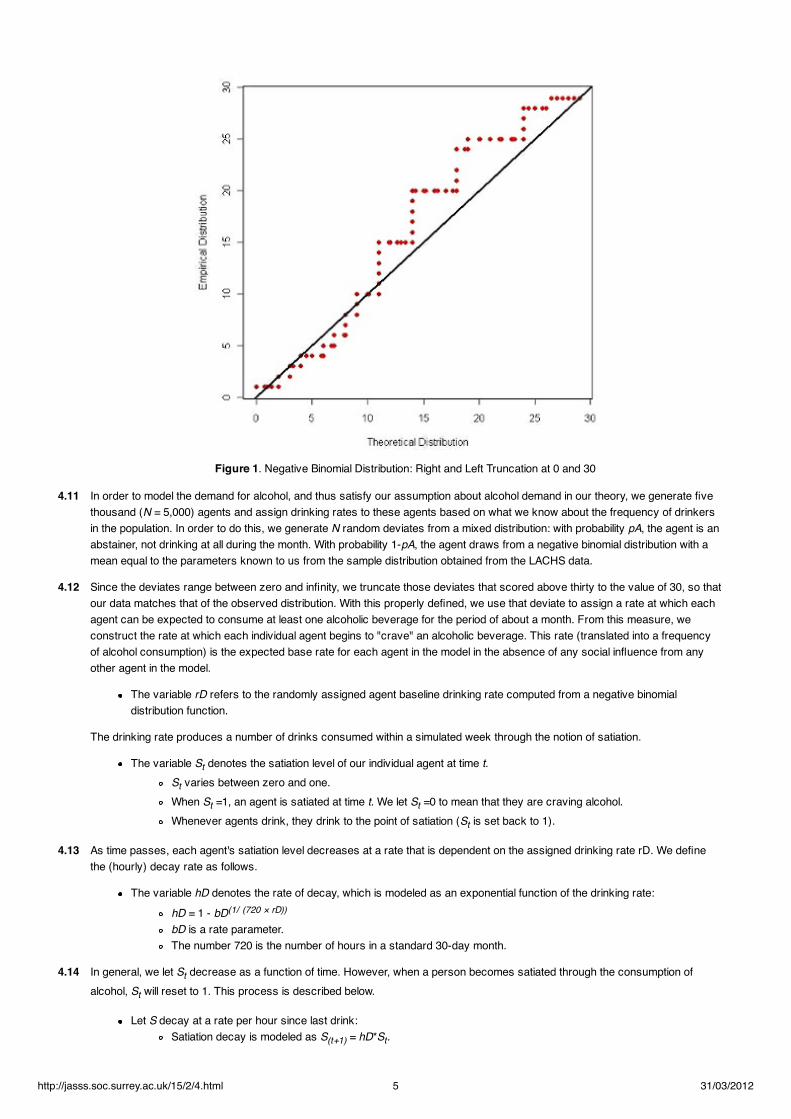
Figure 1. Negative Binomial Distribution: Right and Left Truncation at 0 and 30

4.11 In order to model the demand for alcohol, and thus satisfy our assumption about alcohol demand in our theory, we generate fivethousand (N = 5,000) agents and assign drinking rates to these agents based on what we know about the frequency of drinkersin the population. In order to do this, we generate N random deviates from a mixed distribution: with probability pA, the agent is anabstainer, not drinking at all during the month. With probability 1-pA, the agent draws from a negative binomial distribution with amean equal to the parameters known to us from the sample distribution obtained from the LACHS data.

4.12 Since the deviates range between zero and infinity, we truncate those deviates that scored above thirty to the value of 30, so thatour data matches that of the observed distribution. With this properly defined, we use that deviate to assign a rate at which eachagent can be expected to consume at least one alcoholic beverage for the period of about a month. From this measure, weconstruct the rate at which each individual agent begins to "crave" an alcoholic beverage. This rate (translated into a frequencyof alcohol consumption) is the expected base rate for each agent in the model in the absence of any social influence from anyother agent in the model.

The variable rD refers to the randomly assigned agent baseline drinking rate computed from a negative binomialdistribution function.

The drinking rate produces a number of drinks consumed within a simulated week through the notion of satiation.

The variable St denotes the satiation level of our individual agent at time t.St varies between zero and one.When St =1, an agent is satiated at time t. We let St =0 to mean that they are craving alcohol.Whenever agents drink, they drink to the point of satiation (St is set back to 1).

4.13 As time passes, each agent's satiation level decreases at a rate that is dependent on the assigned drinking rate rD. We definethe (hourly) decay rate as follows.

The variable hD denotes the rate of decay, which is modeled as an exponential function of the drinking rate:hD = 1 - bD(1/ (720 × rD))

bD is a rate parameter.The number 720 is the number of hours in a standard 30-day month.

4.14 In general, we let St decrease as a function of time. However, when a person becomes satiated through the consumption ofalcohol, St will reset to 1. This process is described below.

Let S decay at a rate per hour since last drink:Satiation decay is modeled as S(t+1) = hD*St.

http://jasss.soc.surrey.ac.uk/15/2/4.html 5 31/03/2012

When S(t+1) ≤SI, the agent then consumes alcohol to the point of satiation (after which S(t+1) is reset to 1).The parameter SI denotes the satiation level at which an agent will seek to drink in the absence of socialinfluences.The parameter SS denotes the satiation level at which an agent will seek to drink in the presence of socialinfluences.If an agent is invited by a friend to go out and have a drink, he will drink if St ≤ Ss (after which S(t+1) is set to 1).If it is Friday or Saturday, an agent will randomly select some friends and go out to drink if their St score is: St ≤SW. If this is true, then S(t+1) is set to 1.

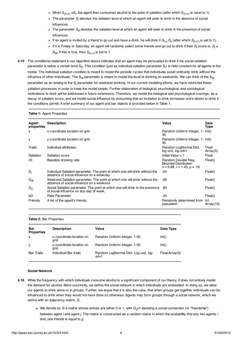
4.15 The conditional statement in our algorithm above indicates that an agent may be persuaded to drink if his social satiationparameter is below a certain level SS. This condition (just as individual satiation parameter SI) is held constant for all agents in themodel. The individual satiation condition is meant to model the periodic cycles that individuals would ordinarily drink without theinfluence of other individuals. The SW parameter is meant to model the level of drinking on weekends. We can think of the SWparameter as an analog to the SI parameter for weekend drinking. In our current modeling efforts, we have restricted thesesatiation processes in order to keep the model simple. Further elaboration of biological, psychological, and sociologicalmotivations to drink will be addressed in future extensions. Therefore, we model the biological and psychological cravings, as adecay of satiation score, and we model social influence by presuming that an invitation to drink increases one's desire to drink ifthe conditions permit. A brief summary of our agent and bar objects is provided below in Table 1.

Table 1: Agent Properties

Agentproperties

Description Value DataType

x x-coordinate location on grid Random Uniform Integer, 1-30

Int()

y y-coordinate location on grid Random Uniform Integer, 1-30

Int()

Traits Individual attributes. Random LogNormal Dist,log u=2, log sd=1

FloatArray(5)

Satiation Satiation score Initial Value = 1 FloatrD Baseline drinking rate Random Deviate Neg.

Binomial Distributionu = 5.88, r = 1.43, p = .19

Float()

SI Individual Satiation parameter. The point at which one will drink without theabsence of social influence on a weekday

.04 Float()

SW Weekend Satiation parameter. The point at which one will drink without theabsence of social influence on a weekend

.60 Float()

SS Social Satiation parameter. The point at which one will drink in the presenceof social influence on any day of week.

.80 Float()

bD Rate Parameter .04 Float()Friends A list of the agent's friends. Randomly determined from

population.IntArray(10)

Table 2: Bar Properties

BarProperties

Description Value Data Type

x x-coordinate location ongrid

Random Uniform Integer, 1-30 Int()

y y-coordinate location ongrid

Random Uniform Integer, 1-30 Int()

Bar Traits Individual Bar traits Random LogNormal Dist. Log u=2, logsd=1

Float Array(5)

Social Network

4.16 While the frequency with which individuals consume alcohol is a significant component of our theory, it does not entirely modelthe demand for alcohol. More succinctly, we define the social network in which individuals are embedded. In doing so, we allowour agents to drink alone or in groups. Further, we argue that it is also the case, that when groups get together individuals can beinfluenced to drink when they would not have done so otherwise. Agents may form groups through a social network, which wedefine with an adjacency matrix, G.

We denote by G a matrix whose entries are either 0 or 1, with Gij=1 denoting a social connection (or "friendship")between agent i and agent j. The matrix is constructed as a random matrix in which the probability that any two agents iand j are friends is equal to g.

http://jasss.soc.surrey.ac.uk/15/2/4.html 6 31/03/2012

4.17 For convenience, we use a random graph to generate the networks. However, the interactions among friends in the network arenot uniform. The model is defined such that agents will tend to go drinking with those in their networks that drink at similar rates.If, for example, an agent has a high propensity to go drinking and one of his friends has a low propensity for drinking, theprobability that the two will go out drinking together will be low. However, if an agent has a friend that drinks at a rate similar to hisown, then the probability that the two will drink will be high.

Agent Traits

4.18 In order to model the ecological niche and assortment strategies among agents, we need to endow agents with abstract traitsthat can be used to model the assortment process. In other words, agents need to be given identities that they can use to assortthemselves into different bars.

Let T be a vector containing m elements identifying m different agent traits. Each of the m elements within this vector arerandom deviates from a trait distribution.Assign a T vector to all N agents in the model.

4.19 In the model, we think of these traits in very abstract terms; more practically, they could represent income, educationalattainment, beverage preference, and any other individual aspects that may affect drinking behavior. We use m=5 traits, eachsampled from a log-normal distribution with a mean log of 2 and standard deviation log of 1, in our simulations below.

4.20 In addition to traits, agents have locations on a two-dimensional plane. That is, we assign geographical positions to agents. The xand y coordinate positions are obtained from a random uniform integer distribution on a discrete rectangular lattice.

Let Ax, Ay refer to each agent's x and y coordinate space on a two-dimensional lattice.

Bar Traits

4.21 Just as with agents, bars occupy a physical location in two-dimensional space.

Let Bx, By refer to each bar's x and y coordinate space on the two-dimensional lattice. These are assigned from arandom uniform integer distribution on a discrete rectangular lattice.

4.22 Lastly, bars, much like our individual agents, carry traits. Unlike the traits of our individual drinkers, bars can change traits inorder to attract particular segments of the drinking population.

Let Nbars refer to the total number of bars in the system.Let B refer to the bar traits. This is a vector containing m elements. This vector is similar to the T vector used to identifyagent traits.

4.23 Each bar attempts to attract a portion of the market share by attempting to match their traits to the traits of the population thatthey are attempting to serve. In order to populate these traits for the bars in the system, we use simple sampling procedures tocompute a score for each of the m elements in B.

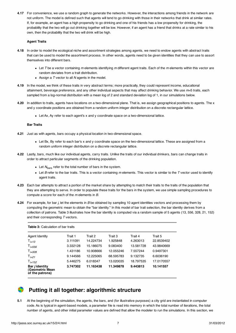
4.24 For example, for bar j, let the elements in B be obtained by sampling 10 agent identities vectors and processing them bycomputing the geometric mean to obtain the "bar identity." In this model of bar trait selection, the bar identity derives from acollection of patrons. Table 3 illustrates how the bar identity is computed via a random sample of 5 agents (13, 556, 328, 21, 152)and their corresponding T vectors.

Table 3: Calculation of bar traits

Agent Identity Trait 1 Trait 2 Trait 3 Trait 4 Trait 5Ti=13 3.111091 14.224734 1.925848 4.263013 22.8539402Ti=556 3.332128 15.186075 9.083400 13.581728 43.9840669Ti=328 1.431186 10.908666 12.055246 7.557244 0.9497301Ti=21 9.144566 12.225065 68.595783 9.132735 6.6036190Ti=152 5.446275 6.018347 13.020035 18.797535 17.0170557Bar j identity(Geometric Mean of the patrons)

3.747302 11.163438 11.349878 9.443813 10.141557

Putting it all together: algorithmic structure5.1 At the beginning of the simulation, the agents, the bars, and (for illustrative purposes) a city grid are instantiated in computer

code. As is typical in agent-based models, a parameter file is read into memory in which the total number of iterations, the totalnumber of agents, and other initial parameter values are defined that allow the modeler to run the simulations. In this section, we

http://jasss.soc.surrey.ac.uk/15/2/4.html 7 31/03/2012

provide psuedocode to illustrate the sequence of steps in terms of how the model is run.

The Social Network

5.2 The simulation begins with a typical workweek beginning on Monday and cycling through the calendar until the simulation modelhas completed a specified number of “computational days.” In order to model the time period, we let each time step in an outerloop represent a 24-hour period. In short, this time period is completed when all individual agents have had the opportunity tomake the decision on whether or not to drink on that day. Each agent individually determines whether or not they desire a drink iftheir satiation score is below SI (Weekday parameter) or SW (Weekend Parameter). They may be influenced to go out for adrink, however, if they are invited to go out drinking with friends. The condition that would allow this possibility to occur is if theirsatiation score is below SS.

5.3 Among those agents that desire an alcoholic beverage, the agents are then selected in random order in which they are thenprovided with the opportunity to select a number of “friends” in their social network to go out and consume alcohol. We call thoseagents that select friends “egos” to denote them as the focal agent. We call those that were selected “alters” to denote thoseagents who were asked to go out to drink.

5.4 The number of agents that an individual agent decides to invite for a drink is determined via a random uniform number generatorthat ranges between 1 and the total number of friends, given that the number of friends are less than or equal to 10. If the totalnumber of friends are greater than 10, then we constrain the individual actor to limit the outing to 10 agents.

5.5 Finally “alter” agents are randomly selected without replacement from the friends of the “ego” agent. Those agents that havesatiation scores less than SS will go drinking with our thirsty agent. For simplicity, invitation events are independently generatedover time; however, one can develop time-dependent models of the invitation process.

5.6 Once it is determined whether or not an agent individually desires an alcoholic beverage, an agent has the opportunity torandomly select a number of drinking partners from their personal network for a drink.

The Selection of Bars

5.7 As mentioned previously, individuals carry with them identities that are used to identify basic demographic characteristics, suchas income, education, beverage choice, and so on. These individual traits could also represent a vast array of any number ofpossible tastes or attributes, such as taste in music, sexual orientation, or even ethnicity. When agents have decided that theywant to go out for an evening, they determine which bar to attend by averaging the geometric mean of their personal traits ontheir T vectors. We call this new vector T'. T' is then compared with the vectors of each individual bar via the standard Euclideandistance measure. In addition to trait comparison, agents also take the spatial location of the bar into consideration. For thesimulations presented herein, we let the agent who did the inviting assist in the selection process. That is, we use the ego'sspatial coordinates to measure the physical distance to each bar.

5.8 In addition, because the actor attributes and the spatial coordinates represent different metrics, we scale the spatial coordinatesand traits with weighting factors. This effect allows the agents to consider spatial location as well as attributes for determiningwhich bar to attend on the landscape.

Determining each Bar's Success

5.9 Each bar will require a certain number of patrons per week in order to maintain financial health. In addition to this requirement, weexpect bar owners will adjust if they see that the number of patrons that they serve drop significantly from the previous week. If abar sees that the number of patrons fall significantly within a week period, then bars may change their attributes in order to adaptto the changing market. If a bar had experienced a loss of clientele that is as large as 50% from the previous week, then the barowner will change attributes.

5.10 We have implemented in this simulation four different strategies for bar proprietors to use in order to maximize their income.

Bar owners will look at the bar that had the most success for that week. In order to improve performance, the bar willcopy the attributes of this bar.Bar owners may sample some fifty individuals (not necessarily patrons of the bar at hand) from the population andcalculate the physical distance of those agents from their bar. Upon calculating this distance, the bar will select thoseagents that are within a given percentile of the distance from the bar. Using these, the bar owner computes the geometricmean of those agents attributes and treats those attributes as the attribute of the bar.The bar owners may randomly sample ten individuals from the population. They will compute the geometric mean fromthat sample to obtain the individual trait characteristics of the population. This algorithm is also currently used to initializebar attributes.Bar owners may select those agent traits that are the least popular and build a bar attribute based on the selection ofthose traits. In here, the bar owners opt for a strategy that seeks to find a niche by focusing on an untapped market.

5.11 Once it has been decided that a bar needs to change attributes, the bar owner will randomly select one of the four strategies with

http://jasss.soc.surrey.ac.uk/15/2/4.html 8 31/03/2012

equal probability of selection.

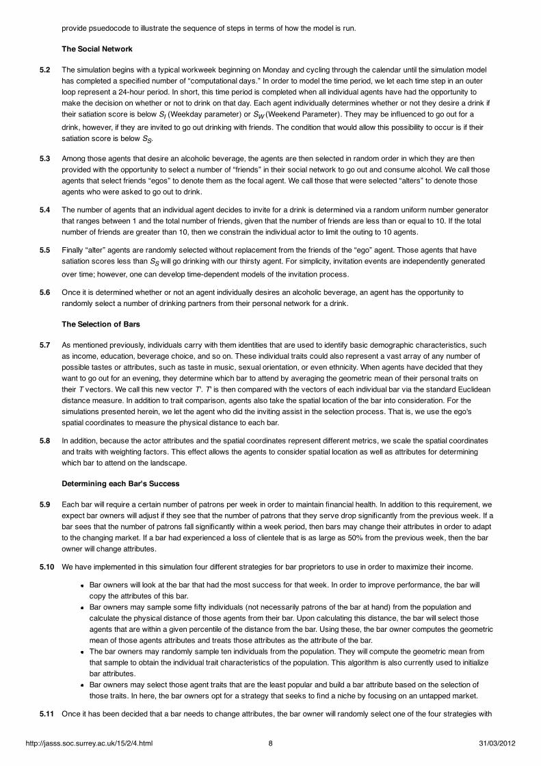
5.12 The entire simulation is encapsulated in the following pseudocode.

//Instantiation of agents and barsInstantiate;

Do while Days ≤ 365;

// Compute Day of Week: Mon - Sun. Days++;

//Allow a 24-hour period to pass: Update Satiation Scores. Sim24Hours; Drinkers = Find_thirsty_agents;

// Permit each ego to invite friends in personal network to drink. // A friend can only be invited to one party per evening. Foreach Ego = Drinkers

If weekday If Ego.sat ≤ Si // Ego randomly selects friends in his // network to join him for a drink. If alters.sat < Ss drink Endif End

If weekend If Ego.sat ≤ Sw // Ego randomly selects friends in his // network to join him for a drink. If alters.sat ≤ Ss drink Endif End

End

// Compute group traits in order to find bars. Compute_group_trait;

// Match Group traits with bar traits. Match_traits.

//Select bar that best matches group traits. Select_bar;

//Reset Satiation scores to 1 Reset_satiation; // If end of week, permit bars to change attributes, // if they desire. Update_bar_traits;

End

Simulations6.1 A total of 174 simulations were conducted in which we systematically studied bar numbers and strategies. We varied the

experimental conditions by starting the models off with 5 bars, and running 5 simulations under those conditions. The next batchof simulations allowed 10 bars to exist, in which we ran the model 5 times under those conditions, and so on. We held all other

http://jasss.soc.surrey.ac.uk/15/2/4.html 9 31/03/2012

variables constant according to the entries denoted in Table 4.

Table 4: Initial Agent Parameter Settings

Variable Name Meaning NumbersN Number of Agents 5000Prob Probability of a friendship .002Nbars Number of bars 5-175Nattr Number of agent and bar attributes 5Niter Total Number of days (iterations) the model is allowed to run. 365GridSize Size of the Lattice: Number of rows and columns. 300 × 300

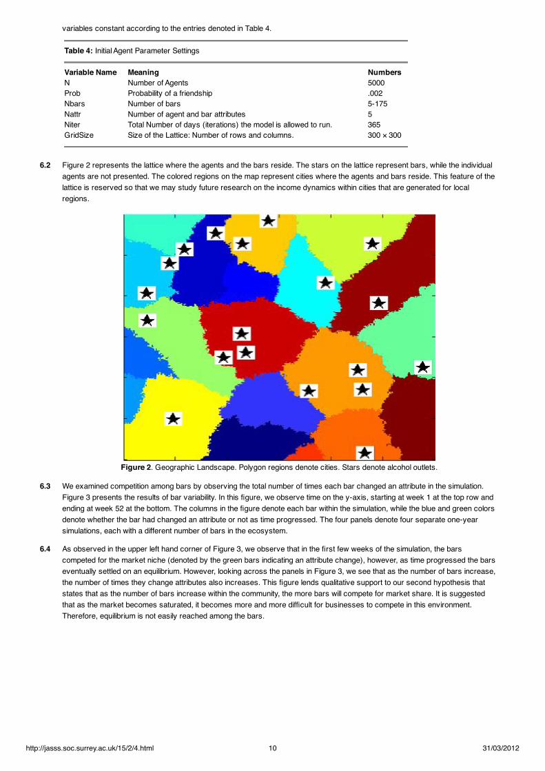
6.2 Figure 2 represents the lattice where the agents and the bars reside. The stars on the lattice represent bars, while the individualagents are not presented. The colored regions on the map represent cities where the agents and bars reside. This feature of thelattice is reserved so that we may study future research on the income dynamics within cities that are generated for localregions.

Figure 2. Geographic Landscape. Polygon regions denote cities. Stars denote alcohol outlets.

6.3 We examined competition among bars by observing the total number of times each bar changed an attribute in the simulation.Figure 3 presents the results of bar variability. In this figure, we observe time on the y-axis, starting at week 1 at the top row andending at week 52 at the bottom. The columns in the figure denote each bar within the simulation, while the blue and green colorsdenote whether the bar had changed an attribute or not as time progressed. The four panels denote four separate one-yearsimulations, each with a different number of bars in the ecosystem.

6.4 As observed in the upper left hand corner of Figure 3, we observe that in the first few weeks of the simulation, the barscompeted for the market niche (denoted by the green bars indicating an attribute change), however, as time progressed the barseventually settled on an equilibrium. However, looking across the panels in Figure 3, we see that as the number of bars increase,the number of times they change attributes also increases. This figure lends qualitative support to our second hypothesis thatstates that as the number of bars increase within the community, the more bars will compete for market share. It is suggestedthat as the market becomes saturated, it becomes more and more difficult for businesses to compete in this environment.Therefore, equilibrium is not easily reached among the bars.

http://jasss.soc.surrey.ac.uk/15/2/4.html 10 31/03/2012

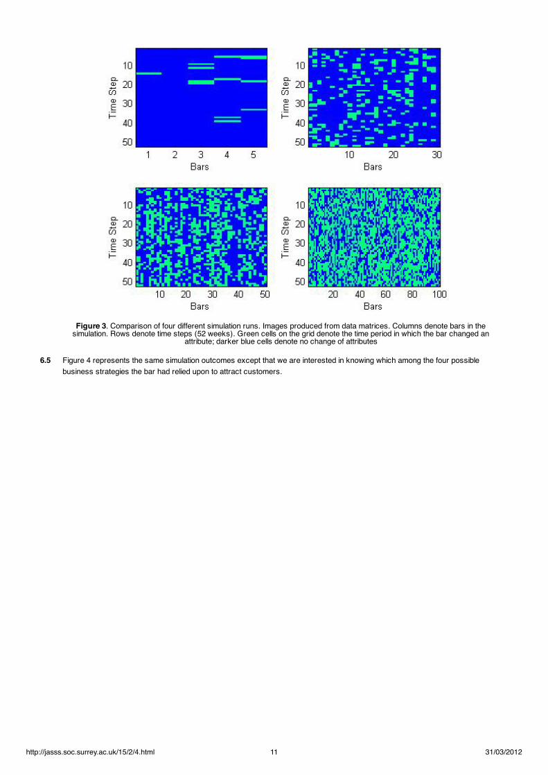
Figure 3. Comparison of four different simulation runs. Images produced from data matrices. Columns denote bars in thesimulation. Rows denote time steps (52 weeks). Green cells on the grid denote the time period in which the bar changed an

attribute; darker blue cells denote no change of attributes

6.5 Figure 4 represents the same simulation outcomes except that we are interested in knowing which among the four possiblebusiness strategies the bar had relied upon to attract customers.

http://jasss.soc.surrey.ac.uk/15/2/4.html 11 31/03/2012

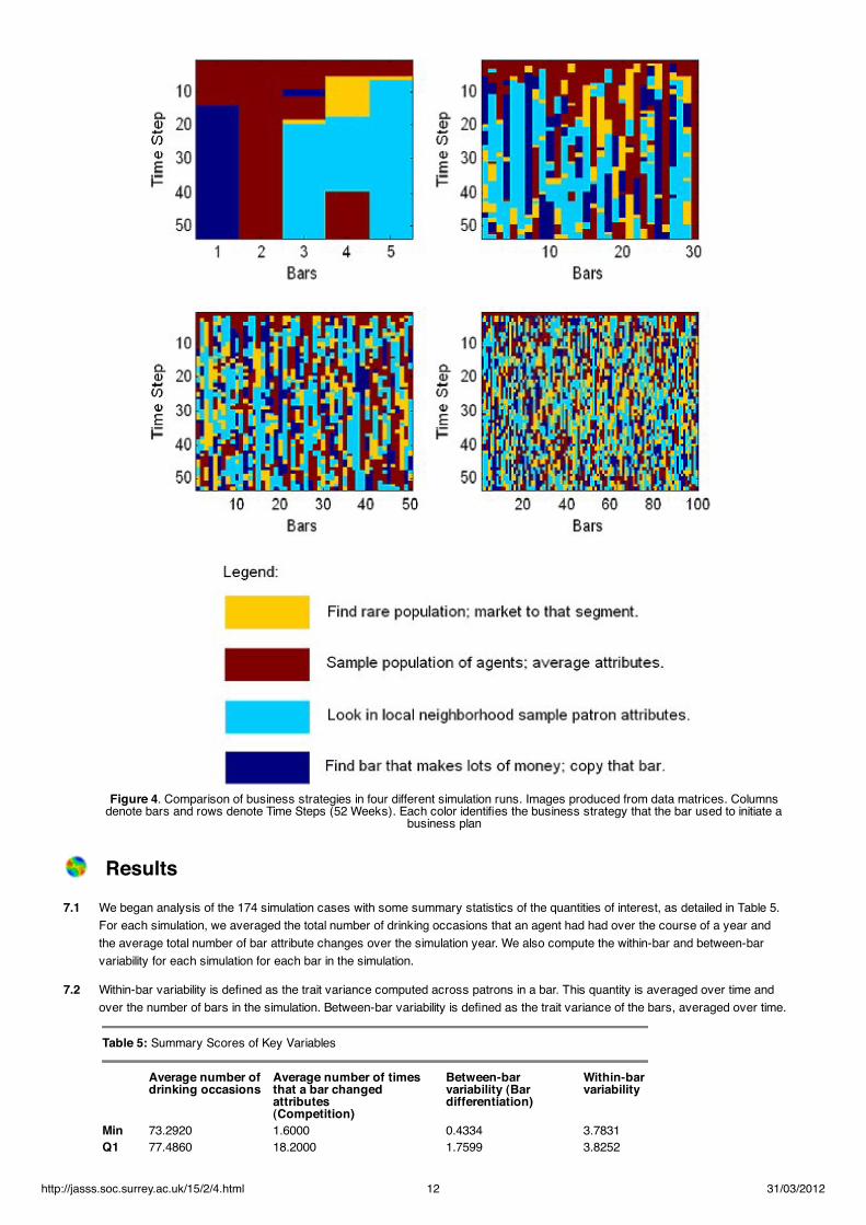
Figure 4. Comparison of business strategies in four different simulation runs. Images produced from data matrices. Columnsdenote bars and rows denote Time Steps (52 Weeks). Each color identifies the business strategy that the bar used to initiate a

business plan

Results7.1 We began analysis of the 174 simulation cases with some summary statistics of the quantities of interest, as detailed in Table 5.

For each simulation, we averaged the total number of drinking occasions that an agent had had over the course of a year andthe average total number of bar attribute changes over the simulation year. We also compute the within-bar and between-barvariability for each simulation for each bar in the simulation.

7.2 Within-bar variability is defined as the trait variance computed across patrons in a bar. This quantity is averaged over time andover the number of bars in the simulation. Between-bar variability is defined as the trait variance of the bars, averaged over time.

Table 5: Summary Scores of Key Variables

Average number ofdrinking occasions

Average number of timesthat a bar changedattributes(Competition)

Between-barvariability (Bardifferentiation)

Within-barvariability

Min 73.2920 1.6000 0.4334 3.7831Q1 77.4860 18.2000 1.7599 3.8252

http://jasss.soc.surrey.ac.uk/15/2/4.html 12 31/03/2012

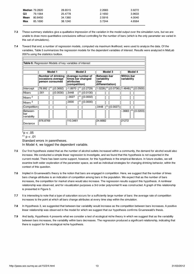
Median 79.2820 28.6515 2.2683 3.9272Q3 79.1564 25.4778 2.1650 3.9633Mean 80.8450 34.1360 2.5916 4.0040Max 85.1690 38.1240 3.7244 4.6564

7.3 These summary statistics give a qualitative impression of the variation in the model output over the simulation runs, but we areunable to draw more quantitative conclusions without controlling for the number of bars (which is the only parameter we varied inthis set of simulations).

7.4 Toward that end, a number of regression models, computed via maximum likelihood, were used to analyze the data. Of thevariables, Table 5 summarizes the regression models for the dependent variables of interest. Results were analyzed in MatLab2007a using the statistics toolbox.

Table 6: Regression Models of key variables of interest

Model 1 Model 2 Model 3 Model 4Number of drinkingoccasions averageperson consumed

Average number oftimes bar changedattributes(competition)

Between-barvariability(bardifferentiation)

Within-barvariability

Intercept 78.992 ** (0.3692) -1.8970 ** (0.2729) 1.0228 ** (0.0736) 1.4848 ** (0.0500)Nbars .001 (0.0030) .5448 ** (0.0130)Nbars 2 -.0027 ** (0.0002)

Nbars 3 .0000 ** (0.0000)Competition .0448 ** (0.0027)Between-barvariability

-.0683 ** (0.0203)

Deviance976.8769 110.3461 24.6682 21272

*p < .05** p < .01Standard errors in parentheses.In Model 4, we logged the dependent variable.

7.5 Our first hypothesis stated that as the number of alcohol outlets increased within a community, the demand for alcohol would alsoincrease. We conducted a simple linear regression to investigate, and we found that this hypothesis is not supported in thecurrent model. There has been some support, however, for this hypothesis in the empirical literature. In future studies, we willexamine both wider exploration of the parameter space, as well as individual strategies for changing drinking behavior, within thecontext of this question.

7.6 Implied in Gruenewald's theory is the notion that bars are engaged in competition. Here, we suggest that the number of timesbars change attributes is an indication of competition among bars in the population. We expect that as the number of barsincreases, the competition for market share would also increase. The regression results support this hypothesis. A nonlinearrelationship was observed, and for visualization purposes a 3rd order polynomial fit was constructed. A graph of this relationshipis presented in Figure 5.

7.7 It is interesting to note that a type of saturation occurs for a sufficiently large number of bars: the average rate of competitionincreases to the point at which all bars change attributes at every time step within the simulation.

7.8 In Hypothesis 3, we suggested that between-bar variability would increase as the competition between bars increases. A positivelinear relationship was observed in the model for which we suggest that our hypothesis confirms Gruenewald's thesis.

7.9 And lastly, Hypothesis 4 presents what we consider a test of ecological niche theory in which we suggest that as the variabilitybetween bars increases, the variability within bars decreases. The regression produced a significant relationship, indicating thatthere is support for the ecological niche hypothesis.

http://jasss.soc.surrey.ac.uk/15/2/4.html 13 31/03/2012

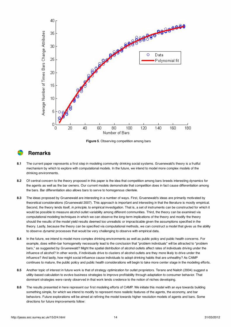
Figure 5. Observing competition among bars

Remarks8.1 The current paper represents a first step in modeling community drinking social systems. Gruenewald's theory is a fruitful

mechanism by which to explore with computational models. In the future, we intend to model more complex models of thedrinking environments.

8.2 Of central concern to the theory proposed in this paper is the idea that competition among bars breeds interesting dynamics forthe agents as well as the bar owners. Our current models demonstrate that competition does in fact cause differentiation amongthe bars. Bar differentiation also allows bars to serve to homogenous clientele.

8.3 The ideas proposed by Gruenewald are interesting in a number of ways. First, Gruenewald's ideas are primarily motivated bytheoretical considerations (Gruenewald 2007). This approach is important and interesting in that the literature is mostly empirical.Second, the theory lends itself, in principle, to empirical investigation. That is, a set of instruments can be constructed for which itwould be possible to measure alcohol outlet variability among different communities. Third, the theory can be examined viacomputational modeling techniques in which we can observe the long-term implications of the theory and modify the theoryshould the results of the model yield results deemed too unrealistic or impracticable given the assumptions specified in thetheory. Lastly, because the theory can be specified via computational methods, we can construct a model that gives us the abilityto observe dynamic processes that would be very challenging to observe with empirical data.

8.4 In the future, we intend to model more complex drinking environments as well as public policy and public health concerns. Forexample, does within-bar homogeneity necessarily lead to the conclusion that “problem individuals” will be attracted to “problembars,” as suggested by Gruenewald? Might the spatial distribution of alcohol outlets affect rates of individuals driving under theinfluence of alcohol? In other words, if individuals drive to clusters of alcohol outlets are they more likely to drive under theinfluence? And lastly, how might social influence cause individuals to adopt drinking habits that are unhealthy? As CAMPcontinues to mature, the public policy and public health considerations will begin to take more center stage in the modeling efforts.

8.5 Another topic of interest in future work is that of strategy optimization for outlet proprietors. Terano and Naitoh (2004) suggest autility-based calculation to evolve business strategies to improve profitability through adaptation to consumer behavior. Thatdominant strategies were rarely observed in that work lends credence to the notion of niches developing.

8.6 The results presented in here represent our first modeling efforts of CAMP. We initiate this model with an eye towards buildingsomething simple, for which we intend to modify to represent more realistic features of the agents, the economy, and barbehaviors. Future explorations will be aimed at refining the model towards higher resolution models of agents and bars. Somedirections for future improvements follow:

http://jasss.soc.surrey.ac.uk/15/2/4.html 14 31/03/2012

In addition to modeling the frequency that individuals drink, we also intend to model how much individuals drink per sitting.We intend to make more use of survey data in order to ground the simulation model. For example, the abstract agentidentities that we had used to construct our agents could be grounded with real attributes (such as age, gender, ethnicity,sexual preference, and so on) that statistically match the observed data in the LACHS survey.Bar owners may act more rationally. Algorithms may be designed so that bar owners may implement techniques to findthe best niche of their choosing. Under this condition, it would be more possible for bar owners to satisfy the drinkingpopulation while also finding economic niches in the spatial environment. This modeling task is closely related to thepreviously defined problem of individual traits.More sophisticated networks of agents will be constructed, in which agents are connected to each other via theirindividual traits (e.g., homophily) and mutual acquaintances.We plan to model outcomes associated with outlet concentrations. We intend to model some of the central tenets thathave concerned alcohol researchers. More specifically, alcohol outlets are often associated with problem areas, such asviolent crime and other negative outcomes. Our major goal of this project is to extend the theory to provide a causalexplanation of problem bars and problem outcomes.

8.7 As observed in our study, the presence of alcohol outlets does not increase alcohol consumption in the overall model. Wesuspect that individuals may decide not to visit bars if the bars are too different from their personal traits. More work is needed torefine these individual and group decisions.

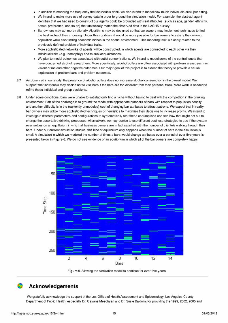
8.8 Under some conditions, bars were unable to satisfactorily find a niche without having to deal with the competition in the drinkingenvironment. Part of the challenge is to ground the model with appropriate numbers of bars with respect to population density,and another difficulty is in the (currently unmodeled) cost of changing bar attributes to attract patrons. We expect that in realitybar owners may utilize more sophisticated techniques or heuristics to maximize their decisions to increase profits. We intend toinvestigate different parameters and configurations to systematically test these assumptions and see how that might set out tochange the assortative drinking processes. Alternatively, we may decide to use different business strategies to see if the systemever settles on an equilibrium in which all business owners are in fact satisfied with the number of clientele walking through theirbars. Under our current simulation studies, this kind of equilibrium only happens when the number of bars in the simulation issmall. A simulation in which we modeled the number of times a bars would change attributes over a period of over five years ispresented below in Figure 6. We do not see evidence of an equilibrium in which all of the bar owners are completely happy.

Figure 6. Allowing the simulation model to continue for over five years

Acknowledgements We gratefully acknowledge the support of the Los Office of Health Assessment and Epidemiology, Los Angeles CountyDepartment of Public Health, especially Dr. Gayane Meschyan and Dr. Susie Baldwin, for providing the 1999, 2002, 2005 and

http://jasss.soc.surrey.ac.uk/15/2/4.html 15 31/03/2012

2007 Los Angeles County Health Survey data. We also greatly appreciate the comments of the reviewers: their observations andsuggestions contributed significantly to this work. This research was supported in part by the Air Force Office of ScientificResearch under grants FA9550-09-1-0524 and FA9550-10-1-0499.

Notes1Similarly, it could be argued that one reason why some individuals may not consume alcohol (or to limit their alcoholconsumption) is because they also believe that it would improve upon their social, emotional, or cognitive net returns.

2Other researchers have also used the number of liters typically consumed within a year (e.g., Skog 1985).

3The mean and scaling parameter were obtained through maximum likelihood estimation. The distribution itself presented a fewpeculiarities, which made distribution fitting unusual. (1) Individuals tended to record their drinking habits based on 5 unitincrements. So, the response categories for 5, 10, 15, 20 tended to have higher frequencies than those response categories inbetween. (2) Zero counts (those who did not drink within that month) were excluded from the distribution. And (3) there is asense in which the distribution was censored at day 30, meaning that those who drank more than thirty days are lumped into the30th day category and so this consequently censors the distribution in a way that it would appear that the distribution was moreheavily biased in one direction. We, therefore, excluded (truncated) those who reported to have drank every day in the last 30days in order to compute these parameters.

References ACKLEH, Azmy S., Ben G. Fitzpatrick, Richard Scribner, Neal Simonsen, Jeremy J. Thibodeaux. (2009). "Ecosystem modelingof college drinking: Parameter estimation and comparing models to data." Mathematical and Computer Modelling, 50(3-4), 481-497.

BICKEL, P., and K. Doksum (1977). Mathematical Statistics: Basic Ideas and Selected Topics, Holden-Day, Oakland.

BULLERS, S., M. Cooper, and M. Russell (2001). Social Network Drinking and Adult Alcohol Involvement: a LongitudinalExploration of the Direction of Influence, Addictive Behaviors 26, 181-199.

CHIU, Arva Y., Pedro E. Perez, Robert Nash Parker (1997). Impact of Banning Alcohol on Outpatient Visits in Barrow, Alaska.Journal of the American Medical Association , 278(21), 1775-1777.

CIARI, Francesco, Michael Löchl, and Kay W. Axhausen (2008). Location decisions of retailers: an agent-based approach. 15thInternational Conference on Recent Advances in Retailing and Services Science, Zagreb, July 2008.

COLLINS, Randall and Robert Hanneman (1998). Modelling the interaction ritual theory of solidarity. In Patrick Doreian andThomas Fararo (Eds.) The Problem of Solidarity: Theories and Models, Gordon and Breach Publishers, Australia.

COX, Miles W. and Eric Klinger (2004). A Motivational Model of Alcohol Use: Determinants of Use and Change, in W. Miles Coxand Eric Klinger (Eds.) Handbook of Motivational Counseling: Concepts, Approaches, and Assessment . John Wiley and Sons,LTD.

CRABB, David W. (1990). Biological markers for increased risk of alcoholism and for quantification of alcohol consumption.Journal of Clicinal Investigations, 85(2), 311-315.

CSIK, B. (2003). Simulation of Competitive Market Situations Using Intelligent Agents, Periodica Polytechnica Ser Soc Man Sci11(1), 83-93.

GORMAN, Dennis M., Jadranka Mezic, Igor Mezic, and Paul J. Gruenewald (2006). Agent-based modeling of drinking behavior:A preliminary model and potential applications to theory and practice. American Journal of Public Health, 96(11), 2055-2060.

GRUENEWALD, Paul J. (2007). The spatial ecology of alcohol problems: niche theory and assortative drinking. Addiction,102(6), 870-878.

HANNEMAN, Robert. (1988). Computer-Assisted Theory Building: Modeling Dynamic Social Systems. Sage Publications, Inc.Newbury Park, CA.

HUANG, Arthur and David Levinson (2011). Why retailers clusters: an agent model of location choice on supply chains.Environment and Planning B: Planning and design, 38(1), 82-94.

JANSSEN, M., and W. Jager (2001). Fashions, Habits, and Changing Preferences: Simulation of Psychological Factors AffectingMarket Dynamics, J. Economic Psychology 22, 745-772.

LEDERMANN, Sully (1956). Alcool, alcoolisme, alcoolisation. Donnés scientifiques de caractére physiologique, économique et

http://jasss.soc.surrey.ac.uk/15/2/4.html 16 31/03/2012

social. Presses Universitaires de France.

LEWIS, Melissa and Clayton Neighbors (2006). Social norms approaches using descriptive drinking norms education: a reviewof the research on personalized normative feedback. Journal of American College Health, 54(4), 213-218.[doi:10.3200/JACH.54.4.213-218 ]

LIVINGSTON, Michael (2008). A Longitudinal Analysis of Alcohol Outlet Density and Assault. Alcoholism: Clinical andExperimental Research, 32(6), 1074-1079. [doi:10.1111/j.1530-0277.2008.00669.x ]

MALLESON, N., L. See, A. Evans, and A. Heppenstall (2012). Implementing comprehensive offender behaviour in a realisticagent-based model of burglary, Simulation 88(1). 50-71. [doi:10.1177/0037549710384124]

MCKINNEY, Christy M., Raul Caetano, Theodore Robert Harris, and Malembe S. Ebama. (2009). Alcohol Availability and IntimatePartner Violence Among US Couples. Alcoholism: Clinical and Experimental Research, 33(1), 169-176. [doi:10.1111/j.1530-0277.2008.00825.x ]

MUNDT JC, Searles, JS, Perrine MW, Helzer JE. (1995). Cycles of alcohol dependence: frequency-domain analyses of dailydrinking logs for matched alcohol-dependent and nondependent subjects. J Stud Alcohol, 56(5), 491-499.

NORTH, Michael J., and Charles M. Macal (2007). Managing Business Complexity: Discovering Strategic Solutions with Agent-Based Modeling and Simulation, Oxford University Press, New York.

NORTH, Michael J., Charles M. Macal, James St. Aubin, Prakash Thimmapuram, Mark Bragen June Hagn, James Karr, NancyBrigham, Mark E. Lacy, and Delaine Hampton. (2010). Multiscale agent-based consumer market modeling. Complexity, 15(5),37-47.

PARKER, Robert Nash, Kate Luther, and Lisa Murphy (2007). Availability, gang violence, and alcohol policy: gaining support foralcohol regulation via harm reduction strategies. Contemporary Drug Problems. 34, 611-633.

PERKINS, H. W., M. P. Haines, et al. (2005). Misperceiving the college drinking norm and related problems: a nationwide study ofexposure to prevention information, perceived norms and student alcohol misuse. J Stud Alcohol, 66(4), 470-478.

PERKINS, H. W., P. W. Meilman, et al. (1999). Misperceptions of the norms for the frequency of alcohol and other drug use oncollege campuses. J Am Coll Health, 47(6), 253-258. [doi:10.1080/07448489909595656 ]

REHM, Jürgen, Tara Kehoe, Gerrit Gmel, Fred Stinson, Bridget Grant, Gerhard Gmel. (2010). Statistical modeling of volume ofalcohol exposure for epidemiological studies of population health: the US example. Population Health Metrics, 8(3), 1-12,http://www.pophealthmetrics.com/content/8/1/3.

ROSENQUIST, J., J. Murabito, J. Fowler, and N. Christakis (2010). The Spread of Alcohol Consumption Behavior in a LargeSocial Network, Annals of Internal Medicine, 152(7), 426-433.

SAID, L. Ben, A. Drogoul, and T. Bouron (2001). A multi-agent based simulation of consumer behaviour: Towards a newmarketing approach. Proceedings of the Interanational Congress on Modelling and Simulation (MODSIM 2001), Canberra,Australia.

SCHENK, Tilman A., Günter Löffler, Jürgen Rauh (2007). Agent-based simulation of consumer behavior in grocery shopping on aregional level. Journal of Business Research, 60(8), 894-903. [doi:10.1016/j.jbusres.2007.02.005]

SCRIBNER, R., A. Ackleh, B. Fitzpatrick, G. Jacquez, J. Thibodeaux, R. Rommel, and N. Simonsen (2009). "EcosystemsModeling of College Drinking: Development of a Deterministic Compartmental Model," J. Studies Alc Drugs , 70(5), 805-821.

SKOG, Ole-Jørgen (1985). The collectivity of Drinking Cultures: A theory of the distribution of alcohol consumption. BritishJournal of Addiction, 80(1), 83-99. [doi:10.1111/j.1360-0443.1985.tb05294.x]

TERANO, T., and K. Naitoh (2004). Agent-Based Modeling for Competing Firms: From Balanced-Scorecards to Multi-ObjectiveStrategies, Proc. 37th Hawaii Intl. Conf. Sys Sci., 1-8

THEALL, Katherine P., Richard Scribner, Bonnie Ghosh-Dastidar, Deborah Cohen, Karen Mason, Neal Simonsen (2009).Neighbourhood alcohol availability and gonorrhea rates: impact of social capital. Geospatial Health 3(2), 241-255.

THOMAS, W. I. (1923). The Unadjusted Girl. Boston: Little, Brown, and Co., 1923.

WECHSLER, Henry, Jae Eun Lee, John Hall, Alexander C. Wagenaar, Hang Lee. 2002. Secondhand effects of student alcoholuse reported by neighbors of colleges: the role of alcohol outlets. Social Science and Medicine. 55, 425-435. [doi:10.1016/S0277-9536(01)00259-3]

WECHSLER, Henry, Toben F. Nelson, Jae Eun Lee, Mark Seibring, Catherine Lewis, and Richard P. Keeling (2003). Perceptionand reality: a national evaluation of social norms marketing interventions to reduce college students' heavy alcohol use. Journalof Studies on Alcohol, 64(3), 484-494.

http://jasss.soc.surrey.ac.uk/15/2/4.html 17 31/03/2012

WEIR, Erica (2003). Seasonal drinking: Let's avoid the 'January effect.' CMAJ, 169(11), 1186-1186.

ZHANG, Tao and David Zhang (2007). Agent-based simulation of consumer purchase decision-making and the decoy effect.Journal of Business Research, 60(8), 912-922. [doi:10.1016/j.jbusres.2007.02.006]

http://jasss.soc.surrey.ac.uk/15/2/4.html 18 31/03/2012