Affective Man-Machine Interface: Unveiling Human Emotions through Biosignals

Affective Man-Machine Interface: Unveiling HumanEmotions through Biosignals

Egon L. van den Broek1, Viliam Lisy2, Joris H. Janssen3,4,Joyce H.D.M. Westerink3, Marleen H. Schut5, and Kees Tuinenbreijer5

1 Center for Telematics and Information Technology (CTIT), University of TwenteP.O. Box 217, 7500 AE Enschede, The Netherlands

[email protected] Agent Technology Center, Dept. of Cybernetics, FEE, Czech Technical University

Technicka 2, 16627 Praha 6, Czech [email protected] User Experience Group, Philips Research

High Tech Campus 34, 5656 AE Eindhoven, The Netherlands{joris.h.janssen,joyce.westerink}@philips.com

4 Dept. of Human Technology Interaction, Eindhoven University of TechnologyP.O. Box 513, 5600 MB, Eindhoven, The Netherlands

[email protected] Philips Consumer Lifestyle Advanced Technology

High Tech Campus 37, 5656 AE Eindhoven, The Netherlands{marleen.schut,kees.tuinenbreijer}@philips.com

Abstract. As is known for centuries, humans exhibit an electrical profile. Thisprofile is altered through various psychological and physiological proce-sses, which can be measured through biosignals; e.g., electromyography (EMG)and electrodermal activity (EDA). These biosignals can reveal our emotions and,as such, can serve as an advanced man-machine interface (MMI) for empathicconsumer products. However, such a MMI requires the correct classification ofbiosignals to emotion classes. This chapter starts with an introduction on biosig-nals for emotion detection. Next, a state-of-the-art review is presented on au-tomatic emotion classification. Moreover, guidelines are presented for affectiveMMI. Subsequently, a research is presented that explores the use of EDA andthree facial EMG signals to determine neutral, positive, negative, and mixed emo-tions, using recordings of 21 people. A range of techniques is tested, which re-sulted in a generic framework for automated emotion classification with up to61.31% correct classification of the four emotion classes, without the need ofpersonal profiles. Among various other directives for future research, the resultsemphasize the need for parallel processing of multiple biosignals.

That men are machines (whatever else they may be) has long been suspected; but not till our gen-eration have men fairly felt in concrete just what wonderful psycho-neuro-physical mechanismsthey are.

William James (1893; 1842 – 1910)

A. Fred, J. Filipe, and H. Gamboa (Eds.): BIOSTEC 2009, CCIS 52, pp. 21–47, 2010.c© Springer-Verlag Berlin Heidelberg 2010

22 E.L. van den Broek et al.

1 Introduction

Despite the early work of William James and others before him, it took more than a cen-tury before emotions became widely acknowledged and embraced by science and en-gineering. However, currently it is generally accepted that emotions cannot be ignored;they influence us, be it consciously or unconsciously, in a wide variety of ways [1]. Letus briefly denote four issues on how emotions influence our lives:

– long term physical well-being; e.g., Repetitive Strain Injury (RSI) [2], cardiovas-cular issues [3,4], and our immune system [5,6];

– physiological reactions / biosignals; e.g., crucial in communication [7,8,9,10];– cognitive processes; e.g., perceiving, memory, reasoning [8,11]; and– behavior; e.g., facial expressions [7,8,12].

As is illustrated by the three ways emotions influence us, we are (indeed) psycho-neuro-physical mechanisms [13,14], who both send and perceive biosignals that can becaptured; e.g., electromyography (EMG), electrocardiography (ECG), and electroder-mal activity (EDA). See Table 1 for an overview. These biosignals can reveal a plethoraof characteristics of people; e.g., workload, attention, and emotions.

In this chapter, we will focus on biosignals that have shown to indicate people’s emo-tional state. Biosignals form a promising alternative for emotion recognition comparedto:

– facial expressions assessed through computer vision techniques [12,15,16]: record-ing and processing is notoriously problematic [16],

– movement analysis [15,17]: often simply not feasible in practice, and– speech processing [12,18,19]: speech is often either absent or suffering from severe

distortions in many real-world applications.

Moreover, biosignals have the advantage that they are free from social masking andhave the potential of being measured by non-invasive sensors, making them suited fora wide range of applications [20,21]. Hence, such biosignals can act as a very usefulinterface between man and machine; e.g., computers or consumer products such asa mp3-player [22]. Such an advanced Man-Machine Interface (MMI) would providemachines with empathic abilities, capable of coping with the denoted issues.

In comparison to other indicators, biosignals have a number of methodological ad-vantages as well. First of all, traditional emotion research uses interviews, question-naires, and expert opinions. These, however, can only reveal subjective feelings, arevery limited in explaining, and do not allow real time measurements: they can onlybe used before or after emotions are experienced [7,8,10]. Second, the recent progressin brain imaging techniques enables the inspection of brain activity while experiencingemotions; e.g., EEG and fMRI [11,28]. Although EEG techniques are slowly brought topractice; e.g., Brain Computer Interfacing (BCI) [29,30], these techniques are still veryobtrusive. Hence, they are not usable in real world situations; e.g., for the integration inconsumer products. As a way between these two research methods, psychophysiologi-cal (or bio)signals can be used [7,8,10,14]. These are not, or at least less, obtrusive, canbe recorded and processed real time, are rich sources of information, and are relativelycheap to apply.

Affective Man-Machine Interface: Unveiling Human Emotions through Biosignals 23

Tabl

e1.

An

over

view

ofco

mm

onbi

osig

nals

/phy

siol

ogic

alsi

gnal

san

dth

eir

feat

ures

,as

used

for

emot

ion

anal

ysis

and

clas

sifi

cati

on

phys

iolo

gyfe

atur

esun

itre

mar

k

card

iova

scul

arac

tivit

y[2

3]he

artr

ate

(HR

)be

ats

/min

thro

ugh

ECG

orBV

PS

DIB

Iss

hear

trat

eva

riab

ilit

y(H

RV

)in

dex

RM

SS

DIB

Iss

hear

trat

eva

riab

ilit

y(H

RV

)in

dex

LF

pow

er(0

.05H

z-

0.15

Hz)

ms2

sym

path

etic

activ

ity

HF

pow

er(0

.15H

z-

0.40

Hz)

ms2

para

sym

path

etic

activ

ity

VL

Fpo

wer

(<

0.05

Hz)

ms2

LF

/HF

puls

etr

ansi

ttim

e(P

TT

)m

sel

ectr

oder

mal

activ

ity

(ED

A)

[24]

mea

n,S

DS

CL

μSto

nic

sym

path

etic

activ

ity

num

ber

ofS

CR

sra

teph

asic

activ

ity

SC

Ram

plit

ude

μSph

asic

activ

ity

SC

R1/

2re

cove

ryti

me

sS

CR

rise

tim

es

skin

tem

pera

ture

[25]

mea

n,S

Dte

mp

oC

(F)

resp

irat

ion

[25]

resp

irat

ion

rate

ampl

itud

ere

spir

atio

ns

resp

irat

ory

sinu

sar

ryth

mia

mus

cle

activ

ity

mea

n,S

Dco

rrug

ator

supe

rcil

iiμV

frow

ning

thro

ugh

EMG

[26,

27]

mea

n,S

Dzy

gom

atic

usm

ajor

μVsm

ilin

g

mea

n,S

Dup

per

trap

eziu

sμV

mea

n,S

Din

ter-

blin

kin

terv

alm

s

Leg

end:

EC

G:

elec

troc

ardi

ogra

m;

BV

P:

bloo

dvo

lum

epu

lse;

EM

G:

elec

trom

yogr

am;

IBI:

inte

r-be

atin

terv

al;

LF

:low

freq

uenc

y;H

F:

high

freq

uenc

y;V

LF

:ve

rylo

wfr

eque

ncy;

SC

L:

skin

cond

ucta

nce

leve

l;S

CR

:sk

inco

nduc

tanc

ere

spon

se;

SD

:st

anda

rdde

viat

ion;

RM

SS

D:

root

mea

nsu

mof

squa

redi

ffer

ence

s.S

eeal

soF

ig.3

for

plot

sof

the

thre

efa

cial

EM

Gsi

gnal

san

dth

eE

DA

sign

al.


A number of prerequisites should be taken into account when using either traditionalmethods (e.g., questionnaires), brain imaging techniques, or biosignals to infer peo-ple’s emotional state. In Van den Broek et al. (2009), these are denoted for affectivesignal processing (ASP); however, most of them also hold for brain imaging, BCI, andtraditional methods. The prerequisites include:

1. the validity of the research employed,2. triangulation; i.e., using multiple information sources (e.g., biosignals) and/or anal-

ysis techniques, and3. inclusion and exploitation of signal processing knowledge ( e.g., determine the

Nyquist frequencies of biosignals for emotion classification).

For a discussion on these topics, we refer to Van den Broek et al. (2009). Let usnow assume that all prerequisites can be satisfied. Then, it is feasible to classify thebiosignals in terms of emotions. In bringing biosignals-based emotion recognition toproducts, self-calibrating, and automatic classification is essential to make it useful forArtificial Intelligence (AI) [1,31], Ambient Intelligence (AmI) [20,32], MMI [7,33],and robotics [34,35].

In the pursuit toward empathic technology, we will describe our work on the auto-matic classification of biosignals. In the next section, we provide an overview of previ-ous work. Section 3 provides an introduction to the classification techniques employed.Subsequently, in Sect. 4, we present the experiment in which we used four biosignalssignals: three facial EMGs and EDA. After that, in Sect. 5, we will briefly introduce thepreprocessing techniques employed. This is followed by Sect. 6 in which the classifi-cation results are presented. In Sect. 7, we reflect on our work and critically review it.Finally, in Sect. 8 we end with drawing the main conclusions.

2 Background

A broad range of biosignals are used in affective sciences; see Table 1. To enable pro-cessing of the signals, in most cases comprehensive sets of features have to be identifiedfor each biosignal; see also Table 2. To extract these features, affective signals are pro-cessed in the time (e.g., statistical moments), frequency (e.g., Fourier), time-frequency(e.g., wavelets), or power domain (e.g., periodogram and autoregression) [36]. In Ta-ble 1, we provide a brief overview of the biosignals most often applied, including theirbest known features, with reference to their physiological source. In the next paragraph,we describe the signals and their psychological counterparts.

First, electrocardiogram (ECG; measured with electrodes on the chest) and bloodvolume pulse (BVP; measured with infra-red light around the finger or ear) can be usedto derive heart beats. The main feature extracted from these heart beats is heart rate(HR; i.e., the number of beats per minute). HR is, however, not very useful in discrim-inating emotions as it is innervated by many different processes. Instead, the heart ratevariability (HRV) provides better emotion information. HRV is more constant in sit-uations where you are happy and relaxed, whereas it shows high variability in morestressful situations [20,55,56]. Second, respiration is often measured with a gauge bandaround the chest. Respiration rate and amplitude mediate the HRV and are, therefore,


Tabl

e2.

An

over

view

of20

stud

ies

onau

tom

atic

clas

sifi

cati

onof

emot

ions

,usi

ngbi

osig

nals

/phy

siol

ogic

alsi

gnal

sg

g/

yg

g

info

rmat

ion

sourc

eye

arsi

gnal

spar

ti-

num

ber

ofse

lect

ion

/cl

assi

fier

sta

rget

clas

sifica

tion

cipan

tsfe

ature

sre

duct

ion

resu

lt

[37]

Sin

ha

&Par

sons

1996

M27

18LD

A2

emot

ions

86%

[9]P

icar

det

al.

2001

C,E,R

,M1

40SFS,Fis

her

LD

A8

emot

ions

81%

[38]

Sch

eire

ret

al.

2002

C,E24

5V

iter

bi

HM

M2

frust

rati

ons

64%

[39]

Nas

ozet

al.

2003

C,E,S

313

k-N

N,LD

A6

emot

ions

69%

[40]

Tak

ahas

hi

2003

C,E,B

1218

SV

M6

emot

ions

42%

[41]

Haa

get

al.

2004

C,E,S

,M,R

113

MLP

vale

nce

/ar

ousa

l64

–97

%[4

2]K

imet

al.

2004

C,E,S

175

10SV

M3

emot

ions

78%

[43]

Lis

etti

&N

asoz

2004

C,E,S

2912

k-N

N,LD

A,M

LP

6em

otio

ns

84%

[44]

Wag

ner

etal

.20

05C,E

,R,M

132

SFS,Fis

her

k-N

N,LD

A,M

LP

4em

otio

ns

92%

[45]

Yoo

etal

.20

05C,E

65

MLP

4em

otio

ns

80%

[46]

Choi

&W

oo20

05E

13

PC

AM

LP

4em

otio

ns

75%

[47]

Hea

ley

&P

icar

d20

05C,E

,R,M

922

Fis

her

LD

A3

stre

ssle

vels

97%

[34]

Liu

etal

.20

06C,E

,M,S

1435

RT

3an

xiet

yle

vels

70%

[48]

Ran

iet

al.

2006

C,E,S

,M,P

1546

k-N

N,SV

M,RT

,B

N3

emot

ions

86%

[49]

Zhai

&B

arre

to20

06C,E

,S,P

3211

SV

M2

stre

ssle

vels

90%

[50]

Jones

&Tro

en20

07C,E

,R13

11A

NN

5ar

ousa

lle

vels

31/

62%

5va

lence

leve

ls26

/57

%[5

1]Leo

net

al.

2007

C,E8

5D

BI

AA

NN

3em

otio

ns

71%

[52]

Liu

etal

.20

08C,E

,S,M

635

SV

M3

affec

tst

ates

83%

[53]

Kat

sis

etal

.20

08C,E

,M,R

1015

SV

M,A

NFIS

4aff

ect

stat

es79

%[5

4]Y

annak

akis

&H

alla

m20

08C,E

7220

AN

OVA

SV

M,M

LP

2fu

nle

vels

70%

[33]

Kim

&A

ndre

2008

C,E,M

,R3

110

SB

SLD

A,D

C4

emot

ions

70/

95%

Sig

nals

:C:c

ardi

ovas

cula

rac

tivit

y;E

:ele

ctro

derm

alac

tivit

y;R

:res

pira

tion

;M:e

lect

rom

yogr

am;B

:ele

ctro

ence

phal

ogra

m;

S:s

kin

tem

pera

ture

;P:p

upil

diam

eter

.cla

ssifi

ers:

ML

P:M

ultiL

ayer

Perc

eptr

on;H

MM

:Hid

den

Mar

kov

Mod

el;R

T:R

egre

ssio

nT

ree;

BN

:Bay

esia

nN

etw

ork;

AN

N:A

rtifi

cial

Neu

ral

Net

wor

k;A

AN

N:A

uto-

Ass

ocia

tive

Neu

ralN

etw

ork;

SV

M:S

uppo

rtV

ecto

rM

achi

ne;

LD

A:L

inea

rD

iscr

imin

antA

naly

sis;

k-N

N:k

-Nea

rest

Nei

ghbo

rs;

AN

FIS

:Ada

ptiv

eN

euro

-Fuz

zyIn

fere

nce

Sys

tem

;DB

I:D

avie

s-B

ould

inIn

dex;

PC

A:P

rinc

ipal

Com

pone

ntA

naly

sis;

SF

S:S

eque

ntia

lFor

war

dS

elec

tion

;S

BS

:Seq

uent

ialB

ackw

ard

Sel

ecti

on;D

C:D

icho

tom

ous

Cla

ssifi

cati

on.


often used in combination, which is called respiratory sinus arrhythmia (RSA) [25].RSA is primarily responsive to relaxation and emotion regulation [57]. Third, electro-dermal activity (EDA) measures the skin conductance of the hands or foots. This isprimarily a response to increases in arousal. Beside the general skin conductance level(SCL), typical peaks in the signal, called skin conductance responses (SCRs), can beextracted. These responses are more event related and are valuable when looking atshort timescales. Fourth, skin temperature, measured at the finger, is also responsive toincreases in arousal, but does not have the typical response peaks as EDA has. Finally,electromyogram (EMG) measures muscle tension. In relation to emotions, this is mostoften applied in the face, where it can measure smiling and frowning [58,59].

When processing such biosignals some general issues have to be taken in considera-tion:

1. Biosignals are typically derived through non-invasive methods to determinechanges in physiology [21] and, as such, are indirect measures. Hence, a delaybetween the actual physiological change and the recorded change in the biosignalhas to be taken into account.

2. Physiological sensors are unreliable; e.g., they are sensitive to movement artifactsand to differences in bodily position.

3. Some sensors are obtrusive, preventing their integration in real world applica-tions [20,22].

4. Biosignals are influenced by (the interaction among) a variety of factors [36,60].Some of these sources are located internally (e.g., a thought) and some are amongthe broad range of possible external factors (e.g., a signal outside). This makes af-fective signals inherently noisy, which is most prominent in real world applications.

5. Physiological changes can evolve in a matter of milliseconds, seconds, minutes oreven longer. Some changes hold for only a brief moment, while others can even bepermanent. Although seldom reported, the expected time windows of change areof interest [20,22]. In particular since changes can add to each other, even whenhaving a different origin.

6. Biosignals have large individual differences. On the one hand, this calls for methodsand models tailored to the individual. It has been shown that personal approachesincrease the performance of ASP [20,33,50]. On the other hand, generic featuresare of the utmost importance. Not in all situations, a system or product can becalibrated. Moreover, directing the quest too fast towards people’s personal profilescould diminish the interest in generic features and, consequently, limit the progressin research towards them.

The features obtained from the biosignals (see Table 1) can be fed to pattern recog-nition methods (see Table 2); cf. [29]. These can be classified as: template matching,syntactic or structural matching, and statistical classification; e.g., artificial neural net-works (ANN). The former two are not or seldom used in ASP, most ASP schemes usethe latter.

Statistical pattern recognition distinguishes supervised and unsupervised (e.g., clus-tering) pattern recognition; i.e., respectively, with or without a set of (labeled) train-ing data [61,62,63]. With unsupervised pattern recognition, the distance / similaritymeasure used and the algorithm applied to generate the clusters are key elements.


Supervised pattern recognition relies on learning from a set of examples (i.e., the train-ing set). Statistical pattern recognition uses input features, a discriminant function (ornetwork function for ANN) to recognize the features, and an error criterion in its clas-sification process.

In the field of ASP, several studies have been conducted, using a broad range ofsignals, features, and classifiers; see Table 2 for an overview. Nonetheless, both therecognition performance and the number of emotions that the classifiers were able todiscriminate are disappointing. Moreover, comparing the different studies is problem-atic because of:

1. The different settings the studies were applied in, ranging from controlled lab stud-ies to real world testing;

2. The type of emotion triggers used;3. The number of target states to be discriminated; and4. The signals and features employed.

To conclude, there is a lack of general standards, low prediction accuracy, and in-consistent results. However, for affective MMI to come to fruition, it is eminent to dealwith these issues. This illustrates the need for a well documented general framework.In this chapter, we set out to initiate its development, explore various possibilities, andapply it on a data set that will be introduced in the next section.

3 Techniques for Classification

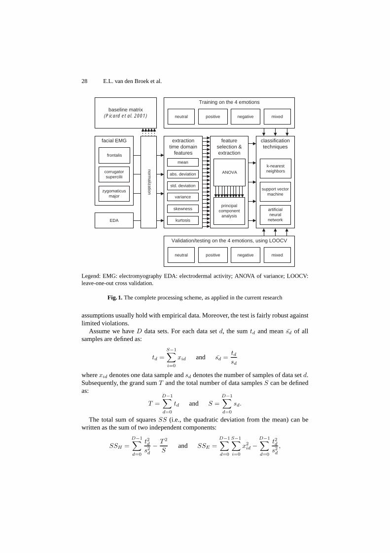
In this section, we briefly introduce the techniques used in the research conducted, forthose readers who are not familiar with them. Figure 1 presents the complete processingscheme of this research. The core of processing scheme consists of three phases, inwhich various techniques were applied.

First, analysis of variance (ANOVA) and principal component analysis (PCA) areintroduced that enabled the selection of a subset of features for the classification ofthe emotions. Second, the classification was done using k-nearest neighbors (k-NN),support vector machines (SVM), and artificial neural networks (ANN), which will bebriefly introduced later in this section. Third and last, the classifiers were evaluatedusing leave-one-out cross validation (LOOCV), which will be introduced at the end ofthis section.

3.1 Analysis of Variance (ANOVA)

Analysis of variance (ANOVA) is a statistical test to determine whether or not there isa significant difference between the means of several data sets. ANOVA examines thevariance of data set means compared to within class variance of the data sets themselves.As such, ANOVA can be considered as an extension of the t-test, which can only beapplied on one or two data sets. We will sketch the main idea here. For a more detailedexplanation, we refer to Chapter 6 of [64].

ANOVA assumes that the data sets are independent and randomly chosen from anormal distribution. Moreover, it assumes that all data sets are equally distributed. These


extractiontime domain

features

facial EMG

frontalis

corrugatorsupercilii

normalizationzygomaticus

major

EDA

mean

abs. deviation

std. deviation

variance

skewness

kurtosis

classificationtechniques

k-nearestneighbors

support vectormachine

artificialneural

network

featureselection &extraction

ANOVA

principalcomponent

analysis

Training on the 4 emotions

positive negative mixedneutral

Validation/testing on the 4 emotions, using LOOCV

positive negative mixedneutral

baseline matrix(Picard et al. 2001)

Legend: EMG: electromyography EDA: electrodermal activity; ANOVA of variance; LOOCV:leave-one-out cross validation.

Fig. 1. The complete processing scheme, as applied in the current research

assumptions usually hold with empirical data. Moreover, the test is fairly robust againstlimited violations.

Assume we have D data sets. For each data set d, the sum td and mean sd of allsamples are defined as:

td =S−1∑i=0

xid and sd =tdsd

where xid denotes one data sample and sd denotes the number of samples of data set d.Subsequently, the grand sum T and the total number of data samples S can be definedas:

T =D−1∑d=0

td and S =D−1∑d=0

sd.

The total sum of squares SS (i.e., the quadratic deviation from the mean) can bewritten as the sum of two independent components:

SSH =D−1∑d=0

t2ds2

d

− T 2

Sand SSE =

D−1∑d=0

S−1∑i=0

x2id −

D−1∑d=0

t2ds2

d

,


where indices H and E denote hypothesis and error, as is tradition in social sciences.Together with S and D, these components define the ANOVA statistic:

F (D − 1, S − D) =S − D

D − 1· SSH

SSE,

where D − 1 and S − D can be considered as the degrees of freedom.The hypothesis that all data sets were drawn from the same distribution is violated if

Fα(D − 1, S − D) < F (D − 1, S − D),

where Fα denotes the ANOVA statistic that accompanies chance level α, considered tobe acceptable. Often α is chosen as either 0.05, 0.01, or 0.001. If α < 0.05 the data setsare assumed to be different.

3.2 Principal Component Analysis (PCA)

Through principal component analysis (PCA), the dimensionality of a data set of in-terrelated variables can be reduced, preserving its variation as much as possible. Thevariables are transformed to a new set of uncorrelated but ordered variables: the prin-cipal components. The first principal component represents, as much as possible, thevariance of the original variables. Each succeeding component represents the remain-ing variance, as much as possible. For a brief introduction on PCA, we refer to Chapter12 of [64].

Suppose we have a set of data, each represented as a vector x, which consists of nvariables. Then, the principal components are defined as a linear combination α · x ofthe variables of x that preserves the maximum of the (remaining) variance, denoted as:

α · x =n−1∑i=0

αixi,

where α = (α0, α1, . . . , αn−1)T . The variance covered by each principal componentα · x is defined as:

var(α · x) = α · Cα,

where C is the covariance matrix of x.To find all principal components, we need to find the maximized var(α ·x) for them.

Hereby, the constraint α ·α = 1 has to be taken into account. The standard approach todo so is the technique of Lagrange multipliers. We maximize

α · Cα − λ

(n−1∑i=0

α2i − 1

)= α · Cα − λ(α · α − 1),

where λ is a Lagrange multiplier. Subsequently, we can derive that λ is an eigenvalueof C and α is its corresponding eigenvector.

Once obtained the vectors α, a transformation can be made that maps all data x toits principal components:

x → (α0 · x, α1 · x, . . . , αn−1 · x)


−0.50

0.5−0.5

00.5

−0.5

0

0.5

(a) Negative versus mixed emotions.

−0.50

0.5−0.5

00.5

−0.5

0

0.5

(b) Neutral versus mixed emotions.

−0.50

0.5−0.5

00.5

−0.5

0

0.5

(c) Neutral versus negative emotions.

−0.50

0.5−0.5

00.5

−0.5

0

0.5

(d) Neutral versus positive emotions.

−0.50

0.5−0.5

00.5

−0.5

0

0.5

(e) Positive versus mixed emotions.

−0.50

0.5−0.5

00.5

−0.5

0

0.5

(f) Positive versus negative emotions.

Fig. 2. Visualization of the first three principal components of all six possible combinations of twoemotion classes. The emotion classes are plotted per two to facilitate the visual inspection.Theplots illustrate how difficult it is to separate even two emotion classes, where separating fouremotion classes is the aim. However, note that the emotion category neutral can be best separatedfrom the other three categories: mixed, negative, and positive emotions, as is illustrated in b), c),and d).

Note that the principal components are sensitive to scaling. In order to tackle thisproblem, the components can be derived from the correlation matrix instead of thecovariance matrix. This is equivalent to extracting the principal components in the de-scribed way after normalization of the original data set to unit variance.

PCA is also often applied for data inspection through visualization, where the prin-cipal components are chosen along the figure’s axes. Figure 2 presents such a visual-ization: for each set of two emotion classes, of the total of four, a plot denoting the firstthree principal components is presented.

3.3 k-Nearest Neighbors (k-NN)

k-nearest neighbors (k-NN) is a very intuitive, simple, and often applied machine learn-ing algorithm. It requires only a set of labeled examples (i.e., data vectors), which formthe training set.


Now, let us assume that we have a training set xl and a set of class labels C. Then,each new vector xi from the data set is classified as follows:

1. Identify k vectors from xl that are closest to vector xi, according to a metric ofchoice; e.g., city block, Euclidean, or Mahalanobis distance.

2. Class ci that should be assigned to vector xi is determined by:

ci = argmaxc∈C

k−1∑i=0

wiγ(c, cli),

where γ(.) denotes a boolean function that returns 1 when c = cli and 0 otherwise

and

wi =

{1 if δ(xi, x

li) = 0;

1d(xi,xl

i)2 if δ(xi, x

li) �= 0,

where δ(.) denotes the distance between vectors xi and xli. Note that, if preferred,

the factor weight can be simply eliminated by putting wi = 1.3. If there is a tie of two or more classes c ∈ C, vector xi is randomly assigned to one

of these classes.

The algorithm presented applies to k-NN for weighted, discrete classifications, as willbe applied in the current research. However, a simple adaptation can be made to thealgorithm, which enables continuous classifications. For more information on these andother issues, we refer to the various freely available tutorials and introductions that havebeen written on k-NN.

3.4 Support Vector Machine (SVM)

Using a suitable kernel function, a support vector machine (SVM) ensures the divisionof a set of data into two classes, with respect to the shape of the classifier and misclas-sification of the training samples. The main idea of SVM can be best explained with theexample of a binary linear classifier.

Let us define our data set as:

D ={(xi, ci)|xi ∈ R

d, ci ∈ {−1, 1}} for i = 0, 1, . . . , N − 1,

where xi is a vector with dimensionality d from the data set, which has size N . ci is theclass to which xi belongs. To separate two classes, we need to formulate a separatinghyperplane w · x = b, where w is a normal vector of length 1, x is a feature vector, andb is a constant.

In practice, it is often not possible to find such a linear classifier. In this case, theproblem can be generalized. Then, we need to find w and b so that we can optimize

ci(w · xi + b) ≤ ξi,

where ξi represents the deviation (or error) from the linearly separable case.To determine an optimal plane, the sum of ξi must be minimized. The minimization

of this parameter can be solved by Lagrange multipliers αi. From the derivation of this


method, it is possible to see that often most of the αis are equal to 0. The remainingrelevant subset of the training data x is denoted as the support vectors. Subsequently,the classification is performed as:

f(x) = sgn

(S−1∑i=0

ciαix · xi + b

),

where S denotes the number of support vectors.For a non-linear classification problem, we can replace the dot product by a non-

linear kernel function. This enables the interpretation of algorithms geometrically infeature spaces non-linearly related to the input space and combine statistics and ge-ometry. A kernel can be viewed as a (non-linear) similarity measure and induce repre-sentations of the data in a linear space. Moreover, the kernel implicitly determines thefunction class, which is used for learning [63].

The SVM introduced here classified samples in two classes. In the case of multipleclasses, two approaches are common: 1) for each class, a classifier can be build thatseparates that class from the other data and 2) for each pair of classes, classifiers canbe build. With both cases, voting paradigms are used to assign the data samples xi toclasses ci. For more information on SVM, [62,63] can be consulted.

3.5 Artificial Neural Networks (ANN)

Artificial neural networks (ANN) are inspired by their biological counterparts. Often,ANN are claimed to have a similar behavior as biological neural networks. AlthoughANN share several features with biological neural networks (e.g., noise tolerance), thisclaim is hardly justified; e.g., a human brain consists of roughly 1011 brain cells, wherean ANN consists of only a few dozens of units.

Nevertheless, ANN have proved their use for a range of pattern recognition and ma-chine learning applications.

Moreover, ANN have a solid theoretical basis [61,62].ANN consist of a layer of input units, one or more layers of hidden units, and a

layer of output units. These units are connected with a weight wij , which determinesthe transfer of unit ui to unit uj . The activation level of a unit uj is defined as:

aj(t + 1) = f(aj(t), ij(t)),

where t denotes time, f(.) is the activation function that determines the new activationbased on the current state a(t) and its effective input, defined as:

ij(t) =Uj−1∑i=0

ai(t)wij(t) + τj(t),

where τj(t) is a certain bias or offset and Uj denotes the number of units from which aunit uj can receive input. Note that at the input layer of a ANN, the input comes fromthe environment; then, i is the environment instead of another unit.


On its own, each neuron of an ANN can only perform a simple task. In contrast, anetwork of units can approximate any function. Moreover, ANN cannot only processinput, they can also learn from their input, either supervised or unsupervised. Althoughvarious learning rules have been introduced for ANN, most can be considered as beingderived from Hebb’s classic learning rule:

Δwij = ηaiaj,

which defines the modification of the weight of connection (ui, uj). η is a positiveconstant. Its rationale is that wij should be increased with the simultaneous activationof both units and the other way around.

Various ANN topologies have been introduced. The most important ones are recur-rent and feed-forward networks, whose units respectively do and do not form a directedcycle through feedback connections. In the current research, a feed-forward networkis applied: the classic multilayer perceptron (MLP), as is more often used for emo-tion recognition purposes; see also Table 2. It incorporated the often adopted sigmoid-shaped function applied to f(.):

11 + e−aj

Throughout the 60 years of their existence, a broad plethora of ANN have beenpresented, varying on a range of aspects; e.g., their topology, learning rules, and thechoice of either synchronous or asynchronously updating of its units. More informationon ANN can be found in various introductions on ANN.

3.6 Leave-One-Out Cross Validation (LOOCV)

Assume we have a classifier that is trained, using a part of the available data set: thetraining data. The training process optimizes the parameters of a classifier to make it fitthe training data. To validate the classifier’s performance, an independent sample of thesame data set has to be used [61,62].

Cross validation deviates from the general validation scheme since it enables the val-idation of a classifier without the need of an explicit validation set. As such, it optimizesthe size of the data set that can be used as training data.

Various methods of cross validation have been introduced. In this section, we willintroduce leave-one-out cross validation (LOOCV), a frequently used method to de-termine the performance of classifiers. LOOCV is typically useful and, consequently,used in the analysis of (very) small data sets. It has been shown that LOOCV providesan almost unbiased estimate of the true generalization ability of a classifier. As such, itprovides a good model selection criterion.

Assume we have a classifier (e.g., k-NN, a SVM, or an ANN) of which we wantto verify its performance on a particular data set. This data set contains (partly) datasamples xi with known correct classifications cl

i. Then, classifier’s performance can bedetermined through LOOCV, as follows:

1. ∀i train a classifier Ci with the complete data set x, except xi.2. ∀i classify data sample xi to a class ci, using classifier Ci.


3. Compute the average error of the classifier through

E =1D

argmaxc∈C

D−1∑i=0

γ(ci, cli),

where D denotes the number of data samples and γ(.) denotes a boolean function,which returns 1 if ci = cl

i and 0 otherwise. Note that 1D can be omitted from the

formula if no comparisons are made between data sets (with different sizes).

Instead of one data sample xi, this validation scheme also allows a subset of the data tobe put aside. Such a subset can, for example, consist of all data gathered of one person.This enables an accurate estimation of the classification error E on this unknown person.

The processing scheme as presented here can be adapted in various ways. For ex-ample, in addition to the boolean function γ(.), a weight function could be used thatexpresses the resemblance between classes. Hence, not all misclassifications would bejudged similarly.

All results reported in this chapter are determined through LOOCV, if not specifiedin another way. For more information on cross validation, LOOCV in particular, werefer to [62].

4 Recording Emotions

We conducted an experiment in which the subjects’ emotions were elicited, using filmfragments that are known to be powerful in eliciting emotions in laboratory settings; seealso [58,59,65]. As biosignals, facial EMG and EDA were recorded. These are knownto reflect emotions [66]; see also both Table 1 and Table 2. The research in which thedata was gathered is already thoroughly documented in both [58] and [59]. Therefore,we will only provide a brief summary of it.

4.1 Participants

In the experiment, 24 subjects (20 females) participated (average age 43 years). Mainlyfemales were solicited to participate since we expected a more and stronger facial emo-tion expression of females [67]. Consequently, a relative small number of males partici-pated. The biosignal recordings of three subjects either failed or were distorted. Hence,the signals of 21 subjects remained for classification purposes.

4.2 Equipment and Materials

We selected 8 film fragments (120 sec. each) for their emotional content. For specifi-cations of these film fragments, see [58,59]. The 8 film fragments were categorized asbeing neutral or triggering positive, negative, or mixed (i.e., simultaneous negative andpositive; [68]) emotions; hence, 2 film fragments per emotion category. This catego-rization was founded on Russell’s valence-arousal model, introduced in [69]. Note thatthe existence of mixed emotions, the way to determine them, and the method to analyzeratings of the possible mixed emotions is still a topic of debate; e.g., [20,22,68].


0

1

2

3

4

5

6

7

8

0 20 40 60 80 100 120

EM

G fr

onta

lis (

μV)

Time (seconds)

0

1

2

3

4

5

6

7

8

0 20 40 60 80 100 120

EM

G c

orru

gato

r su

perc

ilii (

μV)

Time (seconds)

0

1

2

3

4

5

6

7

8

0 20 40 60 80 100 120

EM

G z

ygom

atic

us m

ajor

(μV

)

Time (seconds)

2

2.2

2.4

2.6

2.8

3

0 20 40 60 80 100 120

SC

L (μ

S)

Time (seconds)

Fig. 3. Samples of the electromyography (EMG) in µV of the frontalis, the corrugator supercilii,and the zygomaticus major as well as of the electrodermal activity (EDA) in µV , denoted by theskin conductance level (SCL). All these signals were recorded in parallel, with the same person.

A TMS International Porti5-16/ASD system was used for the biosignal record-ings, which was connected to a PC with TMS Portilab software1. Three facial EMGswere recorded: the right corrugator supercilii, the left zygomaticus major, and the leftfrontalis muscle. The EMG signals were high-pass filtered at 20 Hz, rectified by takingthe absolute difference of the two electrodes, and average filtered with a time constantof 0.2 sec. The EDA was recorded using two active skin conductivity electrodes andaverage filtering with a time constant of about 2 sec. See Fig. 3 for samples of the threeEMG signals and the EDA signal.

4.3 Procedure

After the participant was seated, the electrodes were attached and the recording equip-ment was checked. The 8 film fragments were presented to the participant in pseudo-random order. A plain blue screen was shown between the fragments for 120 seconds.This assured that the biosignals returned to their baseline level, before the next filmfragment was presented.

After the viewing session, the electrodes were removed. Next, the participants an-swered a few questions regarding the film fragments viewed. To jog their memory,representative print-outs of each fragment were provided.

1 URL of TMS Portilab software: http://www.tmsi.com/


5 Preprocessing

The quest towards self-calibrating algorithms for consumer products and for AmI andAI purposes gave some constraints to processing the signals. For example, no advancedfilters should be needed, the algorithms should be noise-resistant, and should (prefer-ably) also be able to handle corrupt data. Therefore, we chose to refrain from advancedpreprocessing schemes and applied basic preprocessing. Figure 1 presents the completeprocessing scheme as applied in the current research.

5.1 Normalization

Humans are known for their rich variety in all aspects, this is no different for theirbiosignals. In developing generic classifiers, this required the normalization of the sig-nals. This was expected to boost its performance significantly [48].

For each person, for all his signals, and for all their features separately, the followingnormalization was applied:

xn =xi − x

σ,

where xn is the normalized value, xi the recorded value, x the global mean, and σ thestandard deviation.

Normalization of data (e.g., signals) has been broadly discussed. This has resulted ina variety of normalization functions; e.g., see [24,61,62].

5.2 Baseline Matrix

In their seminal article, Picard, Vyzas, and Healey (2001) introduced a baseline ma-trix for processing biosignals for emotion recognition. They suggested that this couldtackle problems due to variation both within (e.g., inter day differences) and betweenparticipants. Regrettably, Picard et al. (2001) did not provide evidence for its working.

The baseline matrix requires biosignals recordings while people are in a neutral state.Regrettably, such recordings were not available. Alternatively, one of both availableneutral film fragments was chosen [58,59].

In line with Picard et al. (2001), the input data was augmented with the baseline val-ues of the same data set. A maximum performance improvement of 1.5% was achieved,using a k-NN classifier. Therefore, the baseline matrix was excluded in the final pro-cessing pipeline.

5.3 Feature Selection

To achieve good classification results with pattern recognition and machine learning, theset of input features is crucial. This is no different with classifying emotions [7,8,10].As was denoted in Sect. 2, biosignals can be processed in the time, frequency, time-frequency, and power domain.

For EMG and EDA signals, the time domain is most often employed for featureextraction; see also Table 1. Consequently, we have chosen to explore a range of featuresfrom the time domain: mean, absolute deviation, standard deviation (SD), variance,skewness, and kurtosis. Among these are frequently used features (i.e., mean and SD)


Table 3. The best feature subsets from the time domain, for k-nearest neighbor (k-NN) classifierwith Euclidean metric. They were determined by analysis of variance (ANOVA), using normal-ization per signal per participant. EDA denotes the electrodermal activity or skin conductancelevel.

feature EDA facial electromyography (EMG)frontalis corrugator supercilii zygomaticus

mean oabsolute deviation ostandard deviation (SD) o ovariance o oskewness o o okurtosis o

Table 4. The recognition precision of the k-nearest neighbors (k-NN) classifier, with k = 8 andthe Euclidean metric. The influence of three factors is shown: 1) normalization, 2) analysis ofvariance (ANOVA) feature selection (FS), and 3) Principal Component Analysis (PCA) trans-form.

normalization no fs ANOVA fs ANOVA fs & PCA(10 features) (5 components)

no 45.54%yes 54.07% 60.71% 60.80%

and rarely used, but promising, features (i.e., skewness and kurtosis) [58,59]; see alsoTable 3.

To define an optimal set of features, a criterion function should be defined. How-ever, no such criterion function was available in our case. Thus, an exhaustive searchin all possible subsets of input features (i.e., 224) was required to guarantee an optimalset [70]. To limit this enormous search space, an ANOVA-based heuristic search wasapplied.

For both the normalizations, we performed feature selection based on ANOVAs. Weselected the features with ANOVA α ≤ 0.001 (see also Sect. 3), as this led to the bestprecision. The features selected for each of the biosignals are presented in Table 3.

The last step of preprocessing was PCA; see also Sect. 3. The improvement of thePCA was small compared to feature selection solely. However, it was positive for nor-malization; see also Table 4. Figure 2 presents for each set of two emotion classes, ofthe total of four, a plot denoting the first three principal components. As such, the sixresulting plots illustrate the complexity of separating the emotion classes.

6 Classification Results

This section reports the results of the three classification techniques applied: k-nearestneighbors (k-NN), support vector machines (SVM), and artificial neural networks


Table 5. Confusion matrix of the k-NN classifier of EDA and EMG signals for the best reportedinput preprocessing, with a cityblock metric and k = 8

realneutral positive mixed negative

classified

neutral 71.43% 19.05% 9.52% 14.29%positive 9.52% 57.14% 9.52% 21.43%mixed 4.76% 4.76% 64.29% 11.90%negative 14.29% 19.05% 16.67% 52.38%

(ANN); see also Sect. 3. In all cases, the features extracted from the biosignals wereused to classify participants’ neutral, positive, negative, or mixed state of emotion; seealso Fig. 2. For the complete processing scheme, we refer to Fig. 1.

6.1 k-Nearest Neighbors (k-NN)

For our experiments, we have used MATLAB2 and a k-NN implementation, based onSOM Toolbox 2.03. Besides the classification algorithm described in Sect. 3.3, we haveused a modified version, more suitable for calculating the recognition rates. Its outputwas not the resulting class, but a probability of classification to each of the classes.This means that if there is a single winning class, the output is 100% for the winningclass and 0% for all the other classes. If there is a tie of multiple classes, the outputis divided among them and 0% is provided to the rest. All the recognition rates ofthe k-NN classifier reported in the current study were obtained by using this modifiedalgorithm.

A correct metric is a crucial part of a k-NN classifier. A variety of metrics providedby the pdist function in MATLAB2 was applied. Different feature subsets appearedto be optimal for different classes. Rani et al. (2006) denoted the same issue in theirempirical review; cf. Table 3. The results of the best preprocessed input with respect tothe four emotion classes (i.e., neutral, positive, negative, and mixed) is 61.31%, with acityblock metric and k = 8; cf. Table 4.

Probability tables for the different classifications given a known emotion categoryare quite easy to obtain. They can be derived from confusion matrices of the classifiersby transforming the frequencies to probabilities. Table 5 presents the confusion matrixof the k-NN classifier used in this research, with a cityblock metric and k = 8.

6.2 Support Vector Machines (SVM)

We have used MATLAB2 environment and a SVM and kernel methods toolbox4, forexperimenting with SVMs. We used input enhanced with the best preprocessing, de-scribed in the previous section. It was optimized for the k-NN classifier; however, we

2 MATLAB online: http://www.mathworks.com/products/matlab/3 The MATLAB SOM Toolbox 2.0 is available through:

http://www.cis.hut.fi/projects/somtoolbox4 The SVM and kernel methods toolbox is available through:

http://asi.insa-rouen.fr/enseignants/ arakotom/toolbox/


expected it to be a good input also for more complex classifiers, including SVM. Thisassumption was supported by several tests with various normalizations. Hence, the sig-nals were normalized per person, see also Sect. 5. After feature selection, the first 5principal components from the PCA transformation were selected, see also Sect. 3.

The kernel function of SVM characterizes the shapes of possible subsets of inputsclassified into one category [63]. Being SVM’s similarity measure, the kernel functionis the most important part of an SVM; see also Sect. 3. We applied both a polynomialkernel, with dimensionality d, defined as:

kP (xi, xl) =

(xi · xl

)dand a Gaussian (or radial basis function) kernel, defined as:

kG(xi, xl) = exp

(−|xi − xl|2

2σ2

),

where xi is a feature vector that has to classified and xl is a feature vector assigned to aclass (i.e., the training sample) [63].

A Gaussian kernel (σ = 0.7) performed best with 60.71% correct classification.However, a polynomial kernel with d = 1 had a similar classification performance(58.93%). All the results were slightly worse than with the k-NN classifier.

6.3 Artificial Neural Networks (ANN)

We have used a multi-layer perceptron (MLP) trained by a back-propagation algorithmthat was implemented in the neural network toolbox of MATLAB2; see also Sect. 3. Itused gradient descent with moment and adaptive training parameter. We have tried torecognize only the inputs that performed best with the k-NN classifier.

In order to assess what topology of ANN was most suitable for the task, we con-ducted small experiments with both 1 and 2 hidden layers. In both cases, we did try 5 to16 neurons within each hidden layer. All of the possible 12 + 12 × 12 topologies weretrained, each with 150 cycles and tested using LOOCV.

The experiments using various network topologies supported the claim from [71]that bigger ANN do not always tend to over fit the data. The extra neurons were simplynot used in the training process. Consequently, the bigger networks showed good gen-eralization capabilities but did not outperform the smaller ones. A MLP with 1 hiddenlayer of 12 neurons showed to be the optimal topology.

An alternative method for stopping the adaptation of the ANN is using validationdata. For this reason, the data set was split into 3 parts: 1 subject for testing, 3 subjectsfor validation, and 17 subjects for training. The testing subject was completely removedfrom the training process at the beginning. The network was trained using 17 randomlychosen training subjects. At the end of each training iteration, the network was testedon the 3 validation subjects.

This procedure led to a 56.19% correct classification of the four emotion classes.


6.4 Reflection on the Results

Throughout the last decade, various studies have been presented with similar aims.Some of these studies reported good results on the automatic classification of biosignalsthat should unveil people’s emotions; see Table 2. For example, Picard et al. (2001)reports 81% correct classification on the emotions of one subject [9]. Haag et al. (2004)reports 64%–97% correct classification, using a band function with bandwidth 10% and20%. This study was conducted on one subject. This study reports promising results butalso lacks the necessary details needed for its replication [41]. More recently, Kim andAndre (2008) reported a recognition accuracy of 95% and 70% for subject-dependentand subject-independent classification. Their study included three subjects [33].

In comparison with [9,41,33], this research incorporated data of a large numberof people (i.e., 21), with the aim to develop a generic processing framework. At firstglance, with average recognition rates of 60.71% for SVM and 61.31% for k-NN andonly 56.19% for ANN, its success is questionable. However, the classification ratesdiffer among the four emotion categories, as is shown in Table 5, which presents theconfusion matrix of the results of the k-NN classifier. Neutral emotional states are rec-ognized best, with a classification rate of 71.43%. Negative emotional states are themost complex to distinguish from the other three emotion categories, as is marked byits 52.38% correct classification rate. The complexity of separating the four emotionclasses from each other is illustrated in Fig. 2.

Taking in consideration the generic processing pipeline (see also Fig. 1) and the lim-itations of other comparable research (cf. Table 2), the results reported in this chaptershould be judged as (at least) reasonably good. Moreover, a broad range of improve-ments are possible. One of them would be to question the need of identifying specificemotions, using biosignals for MMI. Hence, the use of alternative, rather rough catego-rizations, as used in the current research, should be further explored.

With pattern recognition and machine learning, preprocessing of the data is crucial.This phase could also be improved for the biosignals used in the current study. First ofall, we think that the feature selection based on an ANOVA was not sufficient for morecomplex classifiers such as neural networks. The ANOVA tests gathered the centersof random distributions that would generate the data of different categories; herebyassuming that their variances were the same. However, a negative result of this test isnot enough to decide that a feature did not contain any information. As an alternative forfeature selection, the k-NN classifier could be extended by a metric that would weighthe features, instead of omitting the confusing or less informative features.

Taken it all together, the quest towards affective MMI continues. Although the resultspresented are good compared to related work, it is hard to estimate whether or not theclassification performance is sufficient for embedding of affective MMI in real worldapplications. However, the future is promising with the rapidly increasing amount ofresources allocated for affective MMI and the range of improvements that are possi-ble. This assures that the performance on classification of emotions will achieve thenecessary further improvements.


7 Discussion

This chapter has positioned men as machines in the sense that they are psycho-neuro-physical mechanisms [13]. It has to be said that this is a far from new position; it isalready known for centuries, although it was rarely exploited in application orientedresearch. However, in the last decade interest has increased and subareas evolved thatutilized this knowledge. This chapter concerns one of them: affective MMI; or as Picard(1997) coined it: affective computing.

A literature overview is provided of the work done so far, see also Table 1 and Ta-ble 2. In addition, some guidelines on affective MMI are provided; see Sects. 1 and 2.To enable the recognition of these emotions, they had to be classified. Therefore, a briefdescription was provided of the classification techniques used (Sect. 3). Next, a studyis introduced in which three EMG signals and people’s EDA were measured (see alsoFig. 3), while being exposed to emotion inducing film fragments; see Sect. 4. See Fig. 1for an overview of the processing scheme applied in the current research. Subsequently,preprocessing and the automatic classification of biosignals, using the four emotioncategories, were presented in Sect. 5 and Sect. 6.

Also in this research, the differences among participants became apparent. They canbe denoted on four levels; see also Sect. 1. People have different physiological reactionson the same emotions and that people experience different emotions with the samestimuli (e.g., music or films). Moreover, these four levels interact [7,8,14]. Althoughour aim was to develop a generic model, one could question whether or not this can berealized. Various attempts have been made to determine people’s personal biosignals-profile; e.g., [9,14,33,48]. However, no generally accepted standard has been developedso far.

In pursuit to generic affective MMI processing schemes, the notion of time should betaken into consideration, as was already denoted in Sect. 2. This can help to distinguishbetween emotions, moods, and personality [20,72,73]:

1. Emotion: A short reaction (i.e., a matter of seconds) to the perception of a specific(external or internal) event, accompanied by mental, behavioral, and physiologicalchanges [7,10].

2. Moods: A long lasting state, gradually changing, in terms of minutes, hours, or evenlonger. They are experienced without concurrent awareness of their origin and arenot object related. Moods do not directly affect actions; however, they do influenceour behavior indirectly [7,10,74].

3. Personality: People’s distinctive traits and behavioral and emotional characteris-tics. For example, introvert and extrovert persons express their emotions in distinctways. Additionally, also self-reports and physiological indicators / biosignals willbe influenced by people’s personality trait [19,75].

With respect to processing the biosignals, the current research could be extendedby a more detailed exploration of the time windows; e.g., with a span of 10 sec-onds [7,8,10,22]. Then, data from different time frames can be combined and different,better suitable normalizations could be applied to create new features. For example,information concerning the behavior of the physiological signals could be more infor-mative than only the integral features from a large time window. Studying short time


frames could also provide a better understanding on the relation between emotions andtheir physiological correlates / biosignals, see also Table 1.

Other more practical considerations should also be noted. The advances made inwearable computing and sensors facilitates (affective) MMI; e.g., [21]. Last years, var-ious prototypes have been developed, which enable the recording of physiological sig-nals; e.g., [76]. This enables the recordings of various biosignals in parallel. In this way,an even higher probability of correct interpretation can be achieved [7,8,20].

Affective MMI can extent consumer products [22]. For example, a mp3-player couldsense its listener’s emotions and either provide suggestions for other music or automati-cally adapt its playing list to these emotions. In addition, various other applications havebeen proposed, mockups have been presented, and implementations have been made.Three examples of these are clothes with wearable computing, games that tweak itsbehavior and presentation depending on your emotions, and lighting that reacts on oradapts to your mood.

Affective signal processing (ASP) could possibly bring salvation to AI [1,20]. Withunderstanding and sensing emotions, true AI is possibly (and finally) within reach. Cur-rent progress in biomedical and electrical engineering provide the means to conductaffective MMI in an unobtrusive manner and, consequently, gain knowledge about ournatural behavior, a prerequisite for modeling it. As AI’s natural successor, for AmI [20],even more than for AI, emotions play a crucial role in making it a success. Since AmIwas coined by Emile Aarts [32], this has been widely acknowledged and repeatedlystressed; e.g., [20,32].

An extension of MMI is human-robot interaction. With robotics, embodiment isa key factor. Potentially, robots are able to enrich their communication substantiallythrough showing some empathy from time to time. As with AI and AmI, this requiressensing and classification of emotions, as can be conveniently done through biosig-nals [34,35].

Of interest for affective MMI are also the developments in brain-computer interfac-ing (BCI) [29,30]. In time, affective BCI will possibly become within science’s reach.Affective BCI, but also BCI in general, could advance AI, AmI, and human-robot inter-action. Slowly this becomes acknowledged, as is illustrated by a workshop on affectiveBCI, as was held at the IEEE 2009 International Conference on Affective Computingand Intelligent Interaction5. With affective BCI, again both its scientific foundation andits applications will be of interest.

Without any doubt affective MMI has a broad range of applications and can help inmaking various areas more successful. Taking it all together, the results gathered in thisresearch are promising. However, the correct classification rate is below that what isneeded for reliable affective MMI in practice. Providing the range of factors that canbe improved, one should expect that the performance can be boosted substantially. Thatthis is not already achieved is not a good sign; perhaps, still some essential mistakes aremade. One of the mistakes could be the computationally driven approach. A processingscheme that is founded on or at least inspired by knowledge from both biology, inparticular physiology, and psychology could possibly be more fruitful . . .

5 The IEEE 2009 International Conference on Affective Computing and Intelligent Interaction:http://www.acii2009.nl/


8 Conclusions

Affective MMI through biosignals is perhaps the ultimate blend of biomedical engi-neering, psychophysiology, and AI. However, in its pursuit, various other disciplines(e.g., electrical engineering and psychology) should not be disregarded. In parallel, af-fective MMI promotes the quest towards its scientific foundation and screams for itsapplication [7,8,10]. As such, it is next generation science and engineering, which trulybridges the gap between man and machine.

As can be derived from this chapter, still various hurdles have to be taken in the de-velopment of a generic, self-calibrating, biosignal-driven classification framework foraffective MMI. The research and the directives denoted here could help in taking someof these hurdles. When the remaining ones will also be taken; then, in time, the commondenominators of people’s biosignals can be determined and their relation with experi-enced emotions can be further specified. This would mark a new, biosignal-driven, eraof advanced, affective MMI.

Acknowledgements. The authors thank Leon van den Broek (Radboud University Ni-jmegen, The Netherlands / University of Utrecht, The Netherlands), Frans van der Sluis(University of Twente, The Netherlands), and Marco Tiemann (Philips Research, TheNetherlands) for their reviews of this book chapter. Furthermore, we thank the editorsfor inviting us to write a chapter for their book.

References

1. Picard, R.W.: Affective Computing. MIT Press, Boston (1997)2. van Tulder, M., Malmivaara, A., Koes, B.: Repetitive strain injury. The Lancet 369(9575),

1815–1822 (2007)3. Schuler, J.L.H., O’Brien, W.H.: Cardiovascular recovery from stress and hypertension fac-

tors: A meta-analytic view. Psychophysiology 34(6), 649–659 (1997)4. Frederickson, B.L., Manusco, R.A., Branigan, C., Tugade, M.M.: The undoing effect of pos-

itive emotions. Motivation and Emotion 24(4), 237–257 (2000)5. Ader, R., Cohen, N., Felten, D.: Psychoneuroimmunology: Interactions between the nervous

system and the immune system. The Lancet 345(8942), 99–103 (1995)6. Solomon, G.F., Amkraut, A.A., Kasper, P.: Immunity, emotions, and stress with special ref-

erence to the mechanisms of stress effects on the immune system. Psychotherapy and Psy-chosomatics 23(1-6), 209–217 (1974)

7. Fairclough, S.H.: Fundamentals of physiological computing. Interacting with Comput-ers 21(1-2), 133–145 (2009)

8. Mauss, I.B., Robinson, M.D.: Measures of emotion: A review. Cognition and Emotion 23(2),209–237 (2009)

9. Picard, R.W., Vyzas, E., Healey, J.: Toward machine emotional intelligence: Analysis ofaffective physiological state. IEEE Transactions on Pattern Analysis and Machine Intelli-gence 23(10), 1175–1191 (2001)

10. van den Broek, E.L., Janssen, J.H., Westerink, J.H.D.M., Healey, J.A.: Prerequisits for Af-fective Signal Processing (ASP). In: Encarnacao, P., Veloso, A. (eds.) Biosignals 2009: Pro-ceedings of the International Conference on Bio-Inspired Systems and Signal Processing,Porto – Portugal, pp. 426–433 (2009)


11. Critchley, H.D., Elliott, R., Mathias, C.J., Dolan, R.J.: Neural activity relating to generationand representation of galvanic skin conductance responses: A functional magnetic resonanceimaging study. The Journal of Neuroscience 20(8), 3033–3040 (2000)

12. Zeng, Z., Pantic, M., Roisman, G.I., Huang, T.S.: A survey of affect recognition methods:Audio, visual, and spontaneous expressions. IEEE Transactions on Pattern Analysis and Ma-chine Intelligence 31(1), 39–58 (2009)

13. James, W.: Review: La pathologie des emotions by Ch. Fere. The Philosophical Review 2(3),333–336 (1893)

14. Marwitz, M., Stemmler, G.: On the status of individual response specificity. Psychophysiol-ogy 35(1), 1–15 (1998)

15. Gunes, H., Piccardi, M.: Automatic temporal segment detection and affect recognition fromface and body display. IEEE Transactions on Systems, Man, and Cybernetics – Part B: Cy-bernetics 39(1), 64–84 (2009)

16. Whitehill, J., Littlewort, G., Fasel, I., Bartlett, M., Movellan, J.: Towards practical smiledetection. IEEE Transactions on Pattern Analysis and Machine Intelligence 31(11), 2106–2111 (2009)

17. Daly, A.: Movement analysis: Piecing together the puzzle. TDR – The Drama Review: AJournal of Performance Studies 32(4), 40–52 (1988)

18. Ververidis, D., Kotropoulos, C.: Emotional speech recognition: Resources, features, andmethods. Speech Communication 48(9), 1162–1181 (2006)

19. Van den Broek, E.L.: Emotional Prosody Measurement (EPM): A voice-based evaluationmethod for psychological therapy effectiveness. Studies in Health Technology and Informat-ics (Medical and Care Compunetics) 103, 118–125 (2004)

20. van den Broek, E.L., Schut, M.H., Westerink, J.H.D.M., Tuinenbreijer, K.: Unobtrusive Sens-ing of Emotions (USE). Journal of Ambient Intelligence and Smart Environments 1(3), 287–299 (2009)

21. Gamboa, H., Silva, F., Silva, H., Falcao, R.: PLUX – Biosignals Acquisition and Processing(2010), http://www.plux.info (Last accessed January 30, 2010)

22. van den Broek, E.L., Westerink, J.H.D.M.: Considerations for emotion-aware consumerproducts. Applied Ergonomics 40(6), 1055–1064 (2009)

23. Berntson, G.G., Bigger, J.T., Eckberg, D.L., Grossman, P., Kaufmann, P.G., Malik, M., Na-garaja, H.N., Porges, S.W., Saul, J.P., Stone, P.H., van der Molen, M.W.: Heart rate variabil-ity: Origins, methods, and interpretive caveats. Psychophysiology 34(6), 623–648 (1997)

24. Boucsein, W.: Electrodermal activity. Plenum Press, New York (1992)25. Grossman, P., Taylor, E.W.: Toward understanding respiratory sinus arrhythmia: Relations

to cardiac vagal tone, evolution and biobehavioral functions. Biological Psychology 74(2),263–285 (2007)

26. Fridlund, A.J., Cacioppo, J.T.: Guidelines for human electromyographic research. Psy-chophysiology 23(5), 567–589 (1986)

27. Reaz, M.B.I., Hussain, M.S., Mohd-Yasin, F.: Techniques of EMG signal analysis: detection,processing, classification and applications. Biological Procedures Online 8(1), 11–35 (2006)

28. Grandjean, D., Scherer, K.R.: Unpacking the cognitive architecture of emotion processes.Emotion 8(3), 341–351 (2008)

29. Lotte, F., Congedo, M., Lecuyer, A., Lamarche, F., Arnaldi, B.: A review of classificationalgorithms for EEG-based brain-computer interfaces. Journal of Neural Engineering 4(2),R1–R13 (2007)

30. Bimber, O.: Brain-Computer Interfaces. IEEE Computer 41(10) (2008); [special issue]31. Minsky, M.: The Emotion Machine: Commonsense Thinking, Artificial Intelligence, and the

Future of the Human Mind. Simon & Schuster, New York (2006)32. Aarts, E.: Ambient intelligence: Vision of our future. IEEE Multimedia 11(1), 12–19 (2004)

http://www.plux.info


33. Kim, J., Andre, E.: Emotion recognition based on physiological changes in music listening.IEEE Transactions on Pattern Analysis and Machine Intelligence 30(12), 2067–2083 (2008)

34. Liu, C., Rani, P., Sarkar, N.: Human-robot interaction using affective cues. In: Proceedingsof the 15th IEEE International Symposium on Robot and Human Interactive Communication(RO-MAN 2006), Hatfield, UK, pp. 285–290. IEEE Computer Society, Los Alamitos (2006)

35. Rani, P., Sims, J., Brackin, R., Sarkar, N.: Online stress detection using psychophysiologicalsignals for implicit human-robot cooperation. Robotica 20(6), 673–685 (2002)

36. Cacioppo, J.T., Tassinary, L.G., Berntson, G.: Handbook of Psychophysiology, 3rd edn. Cam-bridge University Press, New York (2007)

37. Sinha, R., Parsons, O.A.: Multivariate response patterning of fear. Cognition and Emo-tion 10(2), 173–198 (1996)

38. Scheirer, J., Fernandez, R., Klein, J., Picard, R.W.: Frustrating the user on purpose: A steptoward building an affective computer. Interacting with Computers 14(2), 93–118 (2002)

39. Nasoz, F., Alvarez, K., Lisetti, C.L., Finkelstein, N.: Emotion recognition from physiolog-ical signals for presence technologies. International Journal of Cognition, Technology andWork 6(1), 4–14 (2003)

40. Takahashi, K.: Remarks on emotion recognition from bio-potential signals. In: Proceedingsof the IEEE International Conference on Systems, Man and Cybernetics, Palmerston North,New Zealand, October 5-8, vol. 2, pp. 1655–1659 (2003)

41. Haag, A., Goronzy, S., Schaich, P., Williams, J.: Emotion recognition using bio-sensors: Firststeps towards an automatic system. In: Andre, E., Dybkjær, L., Minker, W., Heisterkamp, P.(eds.) ADS 2004. LNCS (LNAI), vol. 3068, pp. 36–48. Springer, Heidelberg (2004)

42. Kim, K.H., Bang, S.W., Kim, S.R.: Emotion recognition system using short-term monitoringof physiological signals. Medical & Biological Engineering & Computing 42(3), 419–427(2004)

43. Lisetti, C.L., Nasoz, F.: Using noninvasive wearable computers to recognize human emo-tions from physiological signals. EURASIP Journal on Applied Signal Processing 2004(11),1672–1687 (2004)

44. Wagner, J., Kim, J., Andre, E.: From physiological signals to emotions: Implementing andcomparing selected methods for feature extraction and classification. In: Proceedings of theIEEE International Conference on Multimedia and Expo. (ICME), Amsterdam, The Nether-lands, July 6-8, pp. 940–943 (2005)

45. Yoo, S.K., Lee, C.K., Park, J.Y., Kim, N.H., Lee, B.C., Jeong, K.S.: Neural network basedemotion estimation using heart rate variability and skin resistance. In: Wang, L., Chen, K.,S. Ong, Y. (eds.) ICNC 2005. LNCS, vol. 3610, pp. 818–824. Springer, Heidelberg (2005)

46. Choi, A., Woo, W.: Physiological sensing and feature extraction for emotion recognition byexploiting acupuncture spots. In: Tao, J., Tan, T., Picard, R.W. (eds.) ACII 2005. LNCS,vol. 3784, pp. 590–597. Springer, Heidelberg (2005)

47. Healey, J.A., Picard, R.W.: Detecting stress during real-world driving tasks using physiolog-ical sensors. IEEE Transactions on Intelligent Transportation Systems 6(2), 156–166 (2005)

48. Rani, P., Liu, C., Sarkar, N., Vanman, E.: An empirical study of machine learning techniquesfor affect recognition in human-robot interaction. Pattern Analysis & Applications 9(1), 58–69 (2006)

49. Zhai, J., Barreto, A.: Stress detection in computer users through noninvasive monitoring ofphysiological signals. Biomedical Science Instrumentation 42, 495–500 (2006)

50. Jones, C.M., Troen, T.: Biometric valence and arousal recognition. In: Thomas, B.H. (ed.)Proceedings of the Australasian Computer-Human Interaction Conference (OzCHI), Ade-laide, Australia, pp. 191–194 (2007)

51. Leon, E., Clarke, G., Callaghan, V., Sepulveda, F.: A user-independent real-time emotionrecognition system for software agents in domestic environments. Engineering Applicationsof Artificial Intelligence 20(3), 337–345 (2007)


52. Liu, C., Conn, K., Sarkar, N., Stone, W.: Physiology-based affect recognition for computer-assisted intervention of children with Autism Spectrum Disorder. International Journal ofHuman-Computer Studies 66(9), 662–677 (2008)

53. Katsis, C.D., Katertsidis, N., Ganiatsas, G., Fotiadis, D.I.: Toward emotion recognition incar-racing drivers: A biosignal processing approach. IEEE Transactions on Systems, Man,and Cybernetics–Part A: Systems and Humans 38(3), 502–512 (2008)

54. Yannakakis, G.N., Hallam, J.: Entertainment modeling through physiology in physical play.International Journal of Human-Computer Studies 66(10), 741–755 (2008)

55. Task Force: Heart rate variability: Standards of measurement, physiological interpretation,and clinical use. European Heart Journal 17(3), 354–381 (1996)

56. Ravenswaaij-Arts, C.M.A.V., Kollee, L.A.A., Hopman, J.C.W., Stoelinga, G.B.A., Geijn,H.P.: Heart rate variability. Annals of Internal Medicine 118(6), 436–447 (1993)

57. Butler, E.A., Wilhelm, F.H., Gross, J.J.: Respiratory sinus arrhythmia, emotion, and emotionregulation during social interaction. Psychophysiology 43(6), 612–622 (2006)

58. van den Broek, E.L., Schut, M.H., Westerink, J.H.D.M., van Herk, J., Tuinenbreijer, K.:Computing emotion awareness through facial electromyography. In: Huang, T.S., Sebe, N.,Lew, M., Pavlovic, V., Kolsch, M., Galata, A., Kisacanin, B. (eds.) ECCV 2006 Workshopon HCI. LNCS, vol. 3979, pp. 52–63. Springer, Heidelberg (2006)

59. Westerink, J.H.D.M., van den Broek, E.L., Schut, M.H., van Herk, J., Tuinenbreijer, K.: 14.In: Computing emotion awareness through galvanic skin response and facial electromyogra-phy. Philips Research Book Series, vol. 8, pp. 137–150. Springer, Dordrecht (2008)

60. Cacioppo, J., Tassinary, L.: Inferring psychological significance from physiological signals.American Psychologist 45(1), 16–28 (1990)

61. Mitchell, T.M.: Machine Learning. The McGraw-Hill Companies, Inc., Columbus (1997)62. Bishop, C.M.: Pattern Recognition and Machine Learning. Information Science and Statis-

tics. Springer Science+Business Media, LLC, New York (2006)63. Scholkopf, B., Smola, A.J.: Learning with kernels: Support Vector Machines, Regulariza-

tion, Optimization, and Beyond. In: Adaptive Computation and Machine Learning. The MITPress, Cambridge (2002)

64. Rencher, A.C.: Methods of Multivariate Analysis, 2nd edn. Wiley Series in Probability andStatistics. John Wiley & Sons, Inc., New York (2002)

65. Rottenberg, J., Ray, R.R., Gross, J.J.: 1. In: Emotion elicitation using films, pp. 9–28. OxfordUniversity Press, New York (2007)

66. Kreibig, S.D., Wilhelm, F.H., Roth, W.T., Gross, J.J.: Cardiovascular, electrodermal, andrespiratory response patterns to fear- and sadness-inducing films. Psychophysiology 44(5),787–806 (2007)

67. Kring, A.M., Gordon, A.H.: Sex differences in emotion: Expression, experience, and physi-ology. Journal of Personality and Social Psychology 74(3), 686–703 (1998)

68. Carrera, P., Oceja, L.: Drawing mixed emotions: Sequential or simultaneous experiences?Cognition & Emotion 21(2), 422–441 (2007)

69. Russell, J.A.: A circumplex model of affect. Journal of Personality and Social Psychol-ogy 39(6), 1161–1178 (1980)

70. Cover, T.M., van Campenhout, J.M.: On the possible orderings in the measurement selectionproblem. IEEE Transactions on Systems, Man, and Cybernetics SMC-7(9), 657–661 (1977)

71. Lawrence, S., Giles, C.L., Tsoi, A.: What size neural network gives optimal generalization?Convergence properties of backpropagation. Technical Report UMIACS-TR-96-22 and CS-TR-3617 (April 1996)

72. Barrett, L.F.: Valence as a basic building block of emotional life. Journal of Research inPersonality 40, 35–55 (2006)


73. Russel, J.A., Barrett, L.F.: Core affect, prototypical emotional episodes, and other thingscalled emotion: Dissecting the elephant. Journal of Personality and Social Psychology 26(5),805–819 (1999)

74. Gendolla, G.H.E.: On the impact of mood on behavior: An integrative theory and a review.Review of General Psychology 4(4), 378–408 (2000)

75. Cooper, C.L., Pervin, L.A.: Personality: Critical concepts in psychology, 1st edn. Criticalconcepts in psychology. Routledge, New York (1998)

76. Lukowicz, P.: Wearable computing and artificial intelligence for healthcare applications. Ar-tificial Intelligence in Medicine 42(2), 95–98 (2008)

Affective Man-Machine Interface: Unveiling Human Emotions through Biosignals

Documents

Transcript of Affective Man-Machine Interface: Unveiling Human Emotions through Biosignals