AEC 403 COURSE TITLE: Agricultural Production Economics ...

i

NATIONAL OPEN UNIVERSITY OF NIGERIA

SCHOOL OF SCIENCE AND TECHNOLOGY

COURSE CODE: AEC 403

COURSE TITLE: Agricultural Production Economics and Resources Management

ii

Course Guide

Course Code AEC 403 Course Title Agricultural Production Economics and Resources Management

Amos, T.T. Department of Agricultural Economics and Extension,

Federal University of Technology, PMB 704, Akure, Ondo State.

iii

1.0 INTRODUCTION 1.1 The Course

1.2 Course Aims 1.3 Course Objectives

1.4 Working through the Course 1.5 The Course Material

1.6 Study Units

AEC403: Agricultural Production Economics and Resources Management (3 Units)

1.0 INTRODUCTION Economics has been defined in a variety of ways and has been a subject of controversy among eminent economists. One school of thought defined its

scope to cover consumption, production, exchange and distribution of wealth by men engaged in the ordinary business of life. Production is central to this school of thought as goods and or services are produced for the consumers who are at the other end of the production process. The producer uses some inputs called resources in an important and intricate proportions to produce

the final commodity.

Thus you will be looking at the subject matter of production economics and resource management in this course.

1.1 THE COURSE

This course Guide tells you, in a nutshell, what you should expect from going through this material. The producer makes on daily basis, decisions

which are economic in nature but may look ordinary to others.

Resources are limited in terms of availability and access. The availability does not confer accessibility as this is related to price of the resources and

the income of the entrepreneur. As we look into production theory, we see that, as the individual

entrepreneur tries to satisfy the objective set through the limited resources, the households’’ utility must be in focus.

Production involves costs which could be either variable or fixed. Producers always try to produce the maximum possible, incurring the least cost, so as

to make the maximum gain possible. The difference between the cost of production and the revenue from the sale of output represents the profit of the producer. The producer always aims at maximizing the profit except in

some exceptional cases.

1.2 COURSE AIMS

iv

The aim of this course is to provide an understanding of the economic decision-making process of the firm. The individual unit is part and parcel

of the total economy. His/her decision has some implications for the running of the economy. In this course, we shall link the decisions made by

the producer with the total economy.

1.3 COURSE OBJECTIVES This course, in addition to its aims, is set to achieve some objectives. At the

end of this course, you should be able to: o Understand the nature of the decision making process of an economic

unit. o Know that price is an important determinant of the quantities of

resources committed to the production process. o Describe the different types of elasticities of production.

o Understand the different factors of production. o Appreciate the production environment and some guiding principles o Understand the theory of cost and revenue as it relates to the firm.

o Differentiate between social and economic costs.

1.4 WORKING THROUGH THE COURSE In this course, it is expected of you to devote considerable time to reading

through the material. The content of this material is very thick and this will require you spending some time studying it. This is the reason for the

considerable efforts put into the development of this material in an attempt to make it very readable and comprehensible for you. It is therefore

necessary that you put serious efforts into reading and studying of the material. Again you should avail yourself of the opportunity of being present during the tutorial sessions so that you would be able to compare knowledge

with your colleagues seek clarification on any grey areas of the topic.

1.5 THE COURSE MATERIAL You are to be provided with two major materials namely

Course guide Study Units

You will observe that the course also comes with a list of recommended text books. These text books are however not compulsory for you to acquire or

read. They are necessary as supplement to the course material.

1.6 STUDY UNITS

v

This course is divided into four Modules and each Module is in turn divided

into Units as follows:

MODULE 1: CONCEPTS IN ECONOMICS MODULE 2: THOERY OF PRODUCTION

MODULE 3: THEORY OF COSTS AND REVENUE

MODULE 4: RESOURCE MANAGEMENT

vi

AEC403: Agricultural Production Economics and Resources Management (3 Units)

Course Code AEC 403

Course Title Agricultural Production Economics and Resources Management

Amos, T.T. Department of Agricultural Economics and Extension,

Federal University of Technology, PMB 704, Akure, Ondo State.

vii

MODULE 1: INTRODUCTION TO AGRICULTURAL ECONOMICS

Unit 1: The Field of Agricultural Economics 1.0 Introduction

2.0 Objective 3.1 The Field of Agriculture

3.1.1 Agriculture as an Art 3.1.2 Agriculture as a Science

3.2 The Field of Agricultural Economics 3.0 Conclusion 4.0 Summary

5.0 Tutor Marked Assignment 6.0 References/Further studies

Unit 2: BASIC ECONOMIC CONCEPTS

1.0. Introduction 2.0. Objectives 3.0. Main body

3.1 Basic Economic Concepts 3.1.1 Scarcity

3.1.2 Resources 3.1.3 Allocation

3.1.4 Choice 3.1.5 Specialization

3.1.6 Exchange 3.1.7 Competing Ends and Goals

3.1.8 Opportunity Cost 3.1.9 The Economic Problem

3.2 Economic Study 3.2.1 Microeconomics

3.2.2 Macroeconomics 4.0 Conclusion 5.0 Summary

6.0 Tutor marked Assignment 7.0 References

Unit 3 : Price Systems and Efficiency

1.0 Introduction 2.0 Objective

3.1. The Workings of the Price System 3.2 Limitations of Price System.

3.3 Price system as it Relates to Efficiency 3.4 The role of Prices in a Perfect Market

3.4.1 What and How much to produce 3.4.2 How to Produce

3.4.3 To determine Income Distribution 3.4.4 To Fully Utilize Resources

3.4.5 To Provide an Incentive To Growth. 3.5 Limitations of the Price system in a perfect competitive market

4.0 Conclusion

viii

5.0 Summary 6.0 Tutor Marked Assignment 7.0 References/Further studies

Unit 4: Relationship between Production Economics and other Fields

1.0 Introduction

2.0 Objective 3.0 Peasant Agriculture and agricultural (production) Economics

3.1 Farm management 3.2 Agricultural economics

3.3Peasant Agriculture 3.4Agricultural science

3.5 Analytical tools of production economics 4.0 Conclusion 5.0 Summary

6.0 Tutor Marked Assignment 7.0 References/ Further Readings

MODULE 2: THEORY OF PRODUCTION

UNIT 1: Production and Production Function 1.0 Introduction

2.0 Objective 3.1 Production and Production Function

3.2 Factors of Production 3.2.1 Natural resources

3.2.2 Labour 3.2.3 Capital

3.2.4 Management or Entrepreneurship 3.3 Production Function

3.4 Production in the Short Run 3.4.1 Assumptions under the Short Run and the Long Run Functions

3.4.2 Production in the Short Run 3.4.3 Production in the Long Run

4.0 Conclusion 5.0 Summary


UNIT 2 PRINCIPLES AND CONCEPTS IN PRODUCTION ANALYSIS


3.0 Principles and Terms 3.1 Law of Diminishing Marginal Returns

3.2 Principles of Maximum Profit3.3 Principle of Limited Resources (Equimarginal Principles)

:

3.4 Physical Product 3.4.1 Total Physical Product (TPP):

3.4.1 Average Physical Product (APP): 3.4.3 Marginal Physical Product (MPP):

ix

3.5 Elasticity of Production (Ep): 3.6.1 Total Value Product (TVP)

3.6.2 Average Value Product (AVP) 3.6.3 Marginal Value Product (MVP)

3.6.4 Total Factor Cost (TFC) 3.6.5 Average Factor Cost (AFC)

3.6.6 Marginal Factor Cost (MFC): 3.7 Comparative advantage

3.8 Gross Margin and Farm Profit 4.0 Conclusion 5.0 Summary

6.0Tutor-marked Assignment 7.0 References/Further readings

UNIT 3: ANALYSIS OF PRODUCTION FUNCTION

1.0 Introduction 2.0 Objective 3.0 Main body

3.1 Analysis of Production Functions 3.2 Factor – Product Relationship 3.3 Factor – Factor Relationship 3.4 Product –Product Relationship


6.0 Tutor-marked Assignment 7.0 References/Further readings

UNIT 4: RELATIONSHIPS AMONG INPUTS AND PRODUCTS

1.0 Introduction 2.0 Objectives 3.0 Main Body

3.1 Relationships between Inputs 3.1.1 Constant rate of substitution

3.1.2 Increasing rate of substitution 3.1.3 Decreasing Rate of Substitution

3.2 Relationships between Products 3.2.1 Competitive Products

3.2.2 Complementary Products 3.2.3 Supplementary Products

3.2.4 Joint Products 4.0 Conclusion 5.0 Summary

6.0 Tutor Marked Assignment 7.0 References/Further readings

MODULE 3: THEORY OF COSTS AND REVENUE

UNIT 1: THEORY OF COSTS

1.0 Introduction 2.0 Objective(s)

x

3.1 THEORY OF COSTS 3.1.1 Costs

3.1.2 Cost Function 3.2 Types of Cost 3.2.1 Total Cost

3.2.2 Average Cost 3.2.3 Marginal Cost

3.3 Private and Social Cost 3.0 Conclusion 4.0 Summary

5.0 Tutor marked Assignment. 6.0 References/Further readings

UNIT 2: THEORY OF REVENUE


3.1 Revenue 3.2 Types of Revenue 3.2.1 Total revenue

3.2.2 Average Revenue 3.2.3 Marginal Revenue

3.3 Profit Analysis 4.0. Conclusion

5.0. Summary 6.0 Tutor-marked Assignment

7.0 References/Further readings

MODULE 4: RESOURCE MANAGEMENT Unit 1: Nature and Structure of Farm Resources


3.0 Nature of Farm Resources 3.1 Renewable Resources 3.2 Non renewable resource

3.3 Demand for Farm Input or Resources 3.4 Valuation of Scare resources

3.4.1 Valuation at cost. In this method, the asset’s actual cost of purchase is used. 3.4.2 Valuation at cost or market price.

3.4.3 Valuation at net selling price. 3.4.4 Valuation at cost less depreciation.

3.4.5 Valuation by reproductive value otherwise known as replacement cost. 3.4 Depreciation


6.0 Tutor Marked Assignment 7.0 References/Further Readings

Unit 2: Optimization Techniques

1.0 Introduction 2.0 Objectives

xi

3.0 Linear programming 3.1 Uses of Linear programming

3.2 Components of Linear Programming 3.3 Assumption of Linear programming

3.3 Steps in Linear Programming Problems 3.4 Methods of Solving Linear Programming Problems

3.5 Primal and Dual Linear Programming Model 3.6 Steps Involved in Converting Primal to Dual Problem


6.0 Tutor marked Assignment 7.0 References/Further Readings

1

MODULE 1: INTRODUCTION TO AGRICULTURAL ECONOMICS Unit One

1.0 Introduction

2.0 Objective 3.0 Main Body

3.1 4.0 Conclusion 5.0 Summary


Unit One: The Field of Agricultural Economics

7.0 Introduction The field of agricultural economics has become popular in Nigeria’s

economy and the agricultural industry is in no doubt enjoying the inputs of agricultural economists in the management of scarce resources on the farm. Incidentally, many people do not fully have an understanding of this field of

agriculture. Resources must be adequately managed for achieving organizational goals. Production economics just deals with this aspect.

In this course, you will be taken through the basics of resource use for

achieving the goal of the farmer. However, in this unit some introduction to the field of agriculture is presented as a reminder to what you may have

learnt in other courses. 8.0 Objective

In this unit, it is expected that you should have gone through this unit and be able to:

-understand the various fields of agriculture; -appreciate the different roles each play in the economy

-potentials contribution of the agricultural economist’s to the economy. 9.0 Main body

3.1 The Field of Agriculture Agriculture is a word derived from two Latin words "ager" and

"cultura" meaning "field cultivation”. But the meaning has been expanded with time, thus agriculture is "the art and science of cultivation of crops and rearing of animals for man's use. Agriculture is both a field of study (applied science) and a practice and the process is incomplete until the crop or animal

so-produced gets to the hands of the ultimate consumer. 3.1.1 Agriculture as an Art

As an art or practice, agriculture can be broadly classified into:

2

Crop Production which encompasses all activities relating to land preparation; planting; fertilizer application; weeding, pests and diseases

control or prevention and harvesting of crops. Animal Production, which involves all activities relating to construction of animal houses, feeding, watering, disease and pest control, and harvesting.

Fishery Production which involves pond construction, feeding, disease and pest control harvesting etc.

Marketing This relates to all activities that transpire from the point of initial production to the ultimate consumer. This include processing, that is,

changing the form of the produce to a more acceptable form to the consumer; transportation, packaging, buying and selling, etc.

Financing This involves sourcing funds for the production of both crops and animals either through personal savings, friends or relatives, co-operatives,

Banks, etc. Support Services like engineers making machines that make work easier and more efficient, scientists producing improved technologies, extension agents and government making inputs needed available to the farmer as at

when needed, etc. 3.1.2 Agriculture as a Science

As a field of study, agricultural science can be broadly classified into: Crop Science, Plant Science or Agronomy: This study area involves

breeding of new seed varieties, developing better technology relating to cultural or agronomic practices, adaptation of new crops to other areas other

than their area of origin; developing varieties resistant to pests, diseases, weeds and drought; developing small scale irrigation technologies compatible with the farming systems of the farmers etc. Areas of

specialization include: Irrigation Agronomy, Weed Science, Genetics, Crop breeding, etc.

3.2 The Field of Agricultural Economics Agricultural economics can be defined as the application of economic

principles to the operations of the agricultural sector. It is concerned with the allocation of resources for the achievement of the organizational i.e

agricultural enterprise goal. This definition can be better understood in light of the various areas which the field of agricultural economics covers. These include but not limited to:

Farm organization, inputs availability, input price and competition, appropriate resource combination for achieving organizational goal which

could be maximum output, maximum profit, maximum income, food sufficiency to mention a few. Products from the input combination have to

reach the final destination, the consumers. Agricultural economics therefore is also concerned with the marketing system for the farm products.

Agricultural economics also is concerned with studying the demand for and supply of agricultural products and those of agro-allied industries. Policies

3

and programs of government as regards the general economy and the agricultural sector is dealt with in agricultural economics. The financing of

the various aspects of the production process is an important aspect that agricultural economics dealt with too. This is in relation to the role of the

banking sector and other financial institutions in the overall development of the agricultural sector. It also gets involved in the trading at both the local

and international markets of agricultural products to determine say the competitiveness of a producing nation in view of the General Agreement of

Tariffs and Trade. Agricultural economics finally, is concerned with the effect of climate change on agriculture and the environment.

Generally speaking, agricultural economics deals with the following special

areas which are widely taught: a. Agribusiness management

b. Agricultural policy and development c. Agricultural Finance

d. Agricultural Cooperative Studies e. Agricultural production Economics f. Agricultural Resource Economics

g. Farm management h. Farm Accounting

i. Agricultural project planning and Analysis j. Agricultural marketing

k. International Trade l. Environmental Economics

m. Research Methodology n. Operations Research

From the foregoing, we can see that a sound knowledge of economics is very essential for successfully understanding the field of agricultural

economics

10.0 Conclusion Agricultural economics is concerned with not only the application of

economic principles to the field of resource utilization in the agricultural industry. Other subjects such as mathematics and statistics are relevant in the

agricultural economics. The place of the agricultural economists in the economy cannot therefore be underrated.

11.0 Summary

In this unit we learnt that agriculture could be regarded as an art or a science depending on how one views it. Also we learnt that the field of agricultural

economics is widening by the day as the economy gets developed. There are about 13 special areas where agricultural economics can be studied.

4

12.0 Tutor Marked Assignment

i. Describe the various disciplines which can find usefulness in agricultural economics.

13.0 References/Further studies

i. Adegeye, A.J and J.S. Dittoh. 1982. Essentials of Agricultural Economics. Impact publishers Nig. Ltd. Ibadan. P. 251

ii. Nmadu, J.N and T.T. Amos 2003. An Introduction to Agricultural Economics. Yekabo Educational publishers. P.172.

5

Unit 2: BASIC ECONOMIC CONCEPTS 1.0 Introduction

2.0 Objective 3.0 Main Body 4.0 Conclusion 5.0 Summary


4.0. Introduction

Given the definition of agricultural economics in the previous unit, there is the need to attempt to provide some basic guide to the field of economics for

those who may not have a strong background of economics. In this unit therefore some basic concepts in the field of economics shall be defined. The

economic theory upon which this unit is based aim at constructing models which describe the economic behavior of individual units/entity which could be the consumer, the firm, government agencies as the case may be and their interactions. These interactions create the economic system of say a region,

country or the world (as the world becomes a global village).

In this unit, we shall provide the basic for this scenario i.e. the definition of economic concepts. These concepts have wide range of use in the field of

agricultural economics. To that end, the student is encouraged to take time to understand these concepts fully.

5.0. Objectives At the end of this unit, it is expected that you would be able to:

I. Define basic concepts in economics II. Apply these concepts to day-day activities

III. Relate these concepts to the field of agricultural economics. 6.0. Main body

3.1 Basic Economic Concepts Social Science: There are four main areas of knowledge of studies namely: physical science, natural (biological) sciences, the humanities and the social

sciences. Sometimes they are grouped into just two: namely; the natural sciences and the social sciences.

The areas of social sciences are fields of learning and research primarily concerned with human relationships. Although no simple definition or categorizations can easily be given to this vast area of knowledge, the

disciplines under the group are characterized by their concern for man, his culture and his relationship with his environment. Social sciences are also concerned with intra and inter group relationship as well as individual and

group reaction to changes in the environment when they occur. Subject areas

6

in this group include: economics, sociology, political science, history, anthropology, psychology, etc.

Economics: The word 'economies' was derived from two Greek words,-oikos' and ‘nemein’ meaning "household management." As the years

roll by, the meaning of economics has been broadened to include management of all resources. Economics is therefore a science of how

people choose to use their limited resources (land, labour capital), which have alternative use, to produce, distributee and exchange consumer goods and services. Economics can also be defined as the science of how scare

resources are allocated among competing ends. Economics is the study of social behavior guiding in the allocation of scarce resources to meet the unlimited needs and desires of the individual members

of a given society. Economics seeks to understand how those individuals interact within the

social structure to address key questions about the production and exchange of goods and services. First, how are individual needs and desires

communicated such that the correct mix of goods and services become available? Second, how does a society provide the incentives for these

individuals to participate in the production of these goods? Third, how is production organized such that maximum-possible quantities are made

available given existing resources and production technology? Finally, given that these individuals are at one time involved in the production process and at other times seeking to acquire the goods that have been produced, how are

trading rules and exchange agreements established? The above questions stress the importance of understanding the process

of production. The goal here is to understand the basic features of production without getting mired in great technical detail. This is accomplished by

developing a simple model that maintains the important features of what are otherwise complex, engineering relationships. Production is about the

conversion of scarce resources. 3.1.1 Scarcity

The most important fact of economics is the law of scarcity: there will never be enough resources to meet everyone's wants. Human wants are

unlimited, but the means to satisfy them is limited or scarce. Scarcity occurs when a society's wants exceed the ability of the economy to meet

these wants. A good is said to be scarce if the amount available (offered to users) is less than the amount people want if it would be given away free of charge; while a good is said to be free if the amount available is greater than the amount people want at no price. These scarce goods have alternative uses hence they are allocated to satisfy a need on the basis of their urgency

or where maximum satisfaction would be obtained. 3.1.2 Resources

7

Resources, also known as inputs are means, which are used to produce scarce goods and services. They are also known as factors of production and

include land (land, mineral, water, air etc), human resources or labour (skilled and unskilled), capital and entrepreneurship or management. They are limited in the sense that the demand for them far outweighs supply and

they are not inexhaustible.

8

3.1.3 Allocation Since resources are scarce or limiting, choices must be made and the

resources managed and rationed among competing ends. Decision must be made about whom to receive, and who to be denied, therefore, the resources

are allocated. Allocation is the appointment of resources for a specific purpose or to particular persons or groups to meet specific need.

3.1.4 Choice Choice and scarcity go together. Individuals, businesses and societies

must choose among alternatives. Choice is facilitated by scale of preference, that is, a scale of wants arranged in order of their importance or urgency. The first want on the list is satisfied first before the second one on the list.

The cost of satisfying the first want in place of the second is opportunity cost or alternative forgone. 3.1.5 Specialization

Economics also study how participants in the economy (people, businesses, countries) specialize in tasks to which they are particularly

suited. Specialization creates wealth. Specialization means that people will produce more of particular goods than they consume and that these

surpluses will be exchanged for the goods (which they do not produce) that they want. One reason for specialization is that people have different skills and technological know-how; land and capital and other resources come in

different varieties and productive capacities and capabilities which therefore makes some people or regions better suited to produce certain goods or

services. 3.1.6 Exchange

Exchange complements specialization and enables individuals to trade the goods in which they specialize for those that others specialize.

Specialization is the necessary consequence of a certain propensity in human nature: the propensity to truck, barter and exchange one thing for the other.

Exchange is everywhere, for example, civil servants exchange their specialized labour for money from the employer.

3.1.7 Competing Ends and Goals Economics, as the definition implies, is the study of how the

competition for limited resources by the inexhaustible needs (or unlimited wants) of man are satisfied. The scarce resources must be allocated among

competing ends. Competing ends are the different purposes for which resources are used.

3.1.8 Opportunity Cost Choice is made necessary by scarcity of resources (which have

alternative uses) with which to satisfy man's unlimited wants; that means some alternatives must be forgone. In economics, the cost of satisfying one

want by forgoing another has a cost, which is called opportunity cost. Opportunity cost of a particular action is the loss of the next best alternative.

9

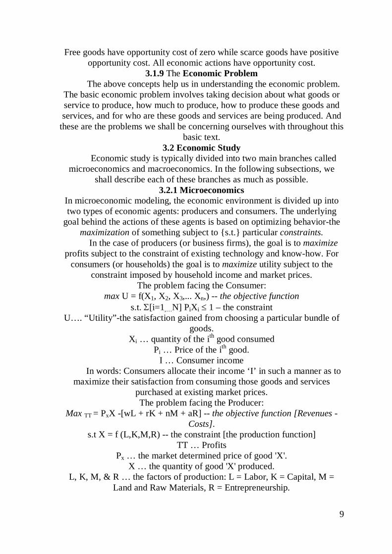
Free goods have opportunity cost of zero while scarce goods have positive opportunity cost. All economic actions have opportunity cost.

3.1.9 The Economic Problem The above concepts help us in understanding the economic problem.

The basic economic problem involves taking decision about what goods or service to produce, how much to produce, how to produce these goods and services, and for who are these goods and services are being produced. And

these are the problems we shall be concerning ourselves with throughout this basic text.

3.2 Economic Study Economic study is typically divided into two main branches called

microeconomics and macroeconomics. In the following subsections, we shall describe each of these branches as much as possible.

3.2.1 Microeconomics In microeconomic modeling, the economic environment is divided up into two types of economic agents: producers and consumers. The underlying

goal behind the actions of these agents is based on optimizing behavior-the maximization of something subject to {s.t.} particular constraints.

In the case of producers (or business firms), the goal is to maximize profits subject to the constraint of existing technology and know-how. For

consumers (or households) the goal is to maximize utility subject to the constraint imposed by household income and market prices.

The problem facing the Consumer: max U = f(X1, X2, X3,... Xn,) -- the objective function

s.t. Σ[i=1,…N] PiXi ≤ 1 – the constraint U…. “Utility”-the satisfaction gained from choosing a particular bundle of

goods. Xi … quantity of the ith good consumed

Pi … Price of the ith good. I … Consumer income

In words: Consumers allocate their income ‘I’ in such a manner as to maximize their satisfaction from consuming those goods and services

purchased at existing market prices. The problem facing the Producer:

Max TT = PxX -[wL + rK + nM + aR] -- the objective function [Revenues - Costs].

s.t X = f (L,K,M,R) -- the constraint [the production function] TT … Profits

Px … the market determined price of good 'X'. X … the quantity of good 'X' produced.

L, K, M, & R … the factors of production: L = Labor, K = Capital, M = Land and Raw Materials, R = Entrepreneurship.

10

W, r, n, & a …factor prices: w = Wages, r = rental cost of capital, n = rents and material prices, a = the normal rate of profit (i.e., the opportunity cost

[next best use] of the entrepreneur’s time). F ( . ) …technology and know-how used to convert the inputs into the

desired output. Producers exist to convert inputs into desired goods and services in an

efficient manner. Given that output prices and factor prices are determined in competitive markets, efficiency means exploiting existing production

technology to the greatest extent possible. Profits earned by the entrepreneur represent the reward for taking risks (facing an uncertain

demand for the output) and achieving efficiency in production (relative to competing producers) - profits that are least equal to what the

entrepreneur could earn by working for someone else. This is the study of economic decision making of firms and

individuals in a market setting. It is the study of the economy in the “small”. It concerns itself with the following: • how consumers behave

• how business firms make choice • how prices are determined in markets

• how taxes and price controls affect consumer and producer behaviour how the structure of the markets affect economic performance

• how wages, interest rates, rent and profits are determined • how income is distributed among families, etc.

The major goal of microeconomics is the achievement of equilibrium price of goods and services in all markets of the economy.

3.2.2 Macroeconomics Economics is a social science that seeks to understand how different

societies allocate resources to meet the unlimited wants and needs of its members. As with any social science, economics is concerned with human

social behavior-behavior of individuals and interaction among these individuals.

The term ‘macro’ was first used in economics by Ragner Frisch at about the year 1933. It is the study of the aggregates in an economy. It

covers aspects such as unemployment, national income, national output, total investment, consumption, savings and supply. Also included is

aggregate demand in the economy, the general price level, wage level and more importantly cost structure. It thus covers the overall dimensions of the economy. In the present day, the issue of unemployment has taken a central stage in many discussions nationally; this is an aspect of macroeconomics.

11

From the foregoing, macroeconomics is the obverse of microeconomics. Though both of them are aggregates, those of the microeconomics are for

example the aggregates of the individual households, firms or industries etc.

Macroeconomics helps to understand the workings of the economy in terms of economic policies, unemployment, national income, monetary policy ( as

we have in the financial sectors now) and business cycles. Many a times however, the static approach is used in macro economics, the dynamic

approach is in wise invalidated. 4.0 Conclusion

Economics study has two branches divisions namely microeconomics and macro economics. Resources are limited and that has necessitated prioritization of wants so as to meet daily challenges of life. These

challenges are in the area of meeting competing needs. Man therefore faces these challenges yet tries to satisfy his goals.

5.0 Summary In this unit we leant that man uses limited resources to meet seemingly

endless competing needs. In the process of defining this, you were told that economics study is concerned with this paradigm and that economics has

two main branches namely microeconomics and macroeconomics. You were also told that while micro deals with the price mechanism which operates with the help of the forces of demand and supply. These forces help to

determine the equilibrium price at the household and at the individual firm levels. Macroeconomics on the other hand, basically concerned with issues

such as at the national income, output and employment which are determined by aggregate demand and supply in the economy.

6.0 Tutor marked Assignment Briefly but concisely define the following concepts and relate them to both

microeconomics and macroeconomics: scarcity, resource, allocation, specialization and opportunity cost

7.0 References i. Adegeye, A.J and J.S. Dittoh. 1982. Essentials of Agricultural Economics.

Impact publishers Nig. Ltd. Ibadan. P. 251 ii. Nmadu, J.N and T.T. Amos 2003. An Introduction to Agricultural

Economics. Yekabo Educational publishers. P.172. iii. Jhingan, M.L. 2008. Macroeconomic Theory. Vrinda publications Limited,

India. P. 787. iv. Jhingan, M.L. 2006. Modern Microeconomics. Vrinda publications Limited,

India.

12

Unit 3 : Price Systems and Efficiency

1.0 Introduction In the previous unit, you were told that there are different types of elasticity. This includes the price elasticity, cross price and income elasticity. In this

Unit, you will find out about how prices are determined and why and when they are high or low.

Everybody is interested in prices either as a producer or a consumer. Price

theory is thus concerned with the economic behavior of consumers, producers, and owners of factors of production. It is concerned with the flow

of goods and services from producers to the consumers.

2.0 Objective It is expected that at the end of this unit, you should be able to:

-Define price theory -understand the limitations of price theory

-Apply the theory of prices to day-to day activities.

3.0 Main Body 3.1. The Workings of the Price System

The price system is that of the economic organization in which the individual engages in economic activities in an atmosphere of freedom. The

individual could be a consumer, a producer or a factor owner. There are legal and social institutions in every society and the economic actions of individuals must conform to these institutions. The price system relates mainly to a perfect competitive system. Individuals own the factors of

production. These individuals have the right to dispose off these factors in accordance with the laws prevailing in the society or country. Thus

individuals have the right to acquire, dispose off, or lease property at will. They have the freedom to enter into contract, to borrow or lend at an agreed

price. Individuals are therefore free to choose any occupation, to buy and sell goods and services from anyone and to anyone based on mutual benefit.

Thus the price system is a system of mutual exchanges and coordination which guide and organize economic activity efficiently, and lead to an

efficient allocation of resources.

3.2 Limitations of Price System. There are some limitations which can be noticed in the price system. Firstly,

there is always an element of uncertainty when constant adjustments are taking in the forces of demand and supply. The process of adjustment is

often painful and costly. Secondly, mistake creep in as the economy is often engulfed in inflationary or deflationary process. If, for example, the supply

13

of resources exceeds the demand for them, in the adjustment process both supply and demand will decrease. So the price system is costly and

uncertain.

3.3 Price system as it Relates to Efficiency Every Price system seeks to attain efficiency with the limited resources at its

disposal. In general therefore, the ability to make the best use of an economy’s available is termed efficiency. There are two major types of

efficiency namely technical and economic efficiency. When an economy is producing the maximum output by making the fullest use of available

resources and technology at its disposal, then the economy is said to be technically efficient. The system is then producing on its production possibility curve. On the other hand an economy achieves economic

efficiency when it is producing the largest possible output of goods and services from its available resources. When the system achieves economic

efficiency, it also achieves technical efficiency and fulfils consumers’ preferences by producing those goods and services that people want with their available incomes. A deviation from this situation is in the sense of a

change in the combination of goods and services will lead to economic inefficiency. It will make someone better off while making another person

worse off.

3.4 The role of Prices in a Perfect Market

In a competitive market, the price mechanism works through supply and demand of goods and services. These, in turn are determined by their prices.

Prices determine the production of innumerable goods and services. They organize production and help in the distribution of goods and services, ration

out the supply of goods and provide for economic growth. There are five basic roles of prices which we shall be considering in this section. Theses

are: o What and How much to produce

o How to Produce o To determine the Distribution of Income

o To Utilize Resources fully o To provide an Incentive to growth

3.4.1 What and How much to produce

Prices help in solving the problem of what to produce and in what quantity should we produce what we want to produce. This is the first role of price. In this case, the allocation of scarce resources in relation to the composition of total output in the economy is considered. Resources are no doubt scarce.

Therefore the society has to decide about the goods to be produced to meet

14

the basic needs of clothing, shelter, food, social amenities such as roads and other infrastructural facilities. Once the nature of goods to be produced is decided, then their quantities are to be decided. For example, how many

million meters of “Nigerian wax”, metric tones of grains such as maize and millet, how many educational institutions, and so on. Since the resources of

the economy are scarce the problem of the nature of goods and their quantities has to be decided on the basis of the priorities of the society. If the society gives priority to the production of more consumer goods now, it will

have less in the future. A higher priority on capital goods implies less consumer goods now and more in the future.

Consumers will have to decide on which of the commodities to purchase. As

they are independent, their taste, priority and income determine to a large extent the level/quantity of goods they will purchase. These thus have effect on the price which in turn has effect on the quantity of goods and services to

produce in the economy.

3.4.2 How to Produce Determination of the technique to use for production is another issue the

price system tries to handle. Every producer aims at using the most efficient productive process. An economically efficient production process is one

which produces goods with the prices of the factor services and the quantity of goods to be produced. A producer uses expensive factor service in smaller

quantity relative to cheap resources.

In order to reduce cost of production, he substitutes cheaper resource for the more expensive one. If capital is relatively cheaper than labour, the

producer will use a capital intensive production process. Contrary wise, if labour is relatively cheaper than capital, labour-intensive production system

will be adopted. In underdeveloped countries where labour is relatively cheap, techniques involving more labour contribute to least cost while in

developed economies where labour is relatively expensive, capital-using and labour-saving techniques combine efficiency with minimum costs. Since one

price for a single commodity prevails in a free enterprise economy, only economically efficient producers can continue in the industry. Those

incapable of paying resources their minimum reward (Prices) will either close down or shift to the manufacture of some other commodity.

3.4.3 To determine Income Distribution

In a free enterprise economy product-distribution and income-distribution are interdependent. It is a system of mutual exchange where the producers

and consumers are largely the same people. Factor owners sell their services for money and then spend that money for purchasing the goods produced by

15

factor services. Producers sell goods and services to consumers for money and consumers receive incomes as factor services owners. Thus income flows from owners of resources (consumers) to producers and back to

consumers. This thus ensures the distribution of income and brings about equality.

3.4.4 To Fully Utilize Resources

The price mechanism helps to ensure full employment of resources of any economy. This can be achieved if there are high investments in the

economy. In a growing economy, equality between saving and investment is brought about by reductions in interest rates. When the economy is

approaching full employment by an efficient use of resources, income then grows at a rapid rate and so do savings. Investments often lags behind whish can be raised to the level of rate by interest-rate reductions. Thus the rate of

interest act as an equilibrating mechanism, however, the rate of interest cannot be relied upon exclusively for this purpose in an economy nearing full employment. Therefore, monetary and fiscal measures, and physical

controls are also required to influence the decisions of consumers and producers regarding saving and investment.

3.4.5 To Provide an Incentive To Growth.

Prices are important factor in enhancing economic growth. The impetus for improvement, innovation and development comes through the price

mechanism. Higher prices and profit encourages large producers to spend large amount of money in research and development to improve and develop

better techniques.

3.5 Limitations of the Price system in a perfect competitive market

The price system does not work perfectly well in a free economy as one may think. Where there are no laws, there would be no offence so there are some

restrictions imposed on the price system directly or indirectly to limit the workings of the price system.

Let us now take a look at them:

i. Government often issues directives to producers so that they would manufacture goods of different types and quantities which are required to

meet the social wants.

ii. At times there are imposition of administrative controls to regulate the supplies of goods, rationing of commodities, issuing of licenses, fixing

quotas and the like are some tools which ensure that the price system does not work freely.

16

iii. Resource owners are not allowed to act freely. If the government allows

the private sector to produce more for the future, then resources will be reallocated towards the capital goods sector. People may also be required to

save more and consume less in the present.

iv. When the government fixes prices of goods and services of say shoes, boxes and others with workers’ wages, these act as constraints on the

operations of the free market mechanism.

v. Social costs such as subsidies also interfere with the working of the price system.

vi. Nationalization policies especially as it affects social services also

tend to modify the price system in favour of mixed economy.

vii. Producers do not always have perfect information as is expected in a perfect market system. They often do not have perfect knowledge of

consumer tastes for instance. These make them to either under produce or overproduce leading to either scarcity or glut in the economy. They therefore

are unable to maximize their profit.

viii. The imperfection of competition also leads to emergence of monopolies which result in wrong pricing, incorrect and wasteful resource

allocation and monopoly profits. These have weakened free competition and reduced consumers’ independence.

ix. Because supply and demand do not work properly, price mechanism has increased income inequalities. Production is guided by the demand of

the elites and often not by the needs of the poor in the society. Resources are therefore directed towards producing luxury goods for the rich who can

afford the price. This further leads to wrong distribution of income.

4.0 Conclusion In this unit you were told that the price system performs five major roles for economic development. These are: What and How much to produce; How to

produce; to determine the Distribution of Income; To Utilize Resources fully; to provide an Incentive to growth. Important as these roles may be

towards economic development, there are some limitations to price mechanism even in a perfect competitive market. Thus price mechanism

does not function freely in economic development as one may think.

5.0 Summary

17

The price system is important for efficiency in any economy be it perfect competitive market or imperfect market. The price mechanism performs

some major roles for efficiency to occur yet there are some limitations to the performance of the roles largely because no government will allow the

economy to be run freely by a system which could lead to a collapse of the economic system.


a. What do you mean by price mechanism? b. Explain the roles of the price mechanism in a competitive economy.

7.0 References/Further studies

1. Jhingan, M.L (2006). Microeconomic Theory. Vrinda Publications Ltd. Delhi.

1. Koutsoyiannis, A. (1984). Modern Microeconomics. Macmillan Publishers. London.

2. Samuelson, P.A. Economics. McMillan, London.

18

Unit 4: Relationship between Production Economics and other Fields


9.0 Peasant Agriculture and agricultural (production) Economics 3.1 Farm management

3.2 Agricultural economics 3.3Peasant Agriculture 3.4Agricultural science

3.5 Analytical tools of production economics 10.0 Conclusion 11.0 Summary


1.0 Introduction

Production economics though a discipline in agricultural economics doe not exist in isolation. In this unit therefore attempt will be made to provide the

basic linkages which the discipline has with other fields of endeavors.

2.0 Objective At the end of this unit, you are expected to :

i. be familiar with other disciplines related to production economics ii. Understand the uniqueness of production economics.

3.0 Peasant Agriculture and agricultural (production) Economics There are some basic disciplines or areas of agriculture that are closely

related to production economics. These are Farm management, Agricultural Economics, Agricultural Science and Peasant Agriculture.

3.1 Farm management Farm management involves application of scientific and technical principles to solving day to day problems on the farm. Agricultural economics grew

out of the interest in farm management on the part of early agricultural technical scientists who tried to develop farm management as a discipline.

These people were mainly interested in the overall operation of the farm as a business and they did not specially relate the discipline of economics until some agricultural scientists who had economic background transferred the

economic theory into the discipline of farm management.

3.2 Agricultural economics

19

Agricultural economics is divided into many sub-disciplines. These sub-disciplines are not mutually exclusive in anyway. They are actually

interdependent. For example the marketing of any commodity may have had its origin in the organization of resource allocation or in financing if not in agricultural extension /education. There is therefore a need to have proper

understanding of the tools of production economics.

3.3Peasant Agriculture This is characterized in Nigeria especially by

i. Farmers operating under small scale level ii. Operated under highly organized system among family members and production is for survival of farm family with little for market to obtain other

household needs not produced on the farm. iii. They use simple farm implements such as hoes and cutlasses appropriately

term hand-tools-technology. iv. Farm holdings are scattered and usually between 0.002 hectare to 2.00

hectare depending on the geographical location. v. Resource utilization is very low leading to low output and productivity, low

capital base. However, there is full utilization of farm assets. vi. Many are with low level of western education and adopt improved

technologies late. vii. There is no full exploitation of the potential capital formation

3.4Agricultural science

There are other disciplines of agriculture as a science which are very closely related also with agricultural economics. These are Animal science, agricultural biochemistry, and nutrition, Agronomy, Soil Science,

Agricultural biology, Agricultural Engineering, and Animal health. All these discipline are working to ensure more food is available for home

consumption and for external markets. The population is ever increasing geometrically and the demand for food and fiber also moving in that direction. Researches are conducted on continuous basis in all these

disciplines to meet up with this trend in population. Though some of them are conducted in an artificial environment, the results must be translated to

farmers’ field which falls within the purview of agricultural economics.

3.5 Analytical tools of production economics Production economics uses explicitly definable variable. These variables rely on quantitative tools for the quantification of and manipulation. This demands the use of mathematical methods such as algebra and differential and integral calculus. Generally production economics use the following

tools in analysis:

20

i. Econometric method. These could be any of Ordinary Least Squares (OLS) or Maximum Likelihood Estimate (MLE) methods.

Simultaneous equations are also relied upon in production economics in addition; statistical principles for hypothesis testing and significance of

parameters are used. These are used for estimating production relationships and thus parameters. Data often used include time series, cross sectional,

panel, experimental and engineering data.

ii. Linear Algebra and its extension to linear programming. The use of this tool is facilitated by the need to provide normative result for policy

formulation, learning and daily decision making process.

iii. Conventional tools of Farm management. These include straight and partial budgeting and the benefit cost analysis. Others are Leontief model of

input-output inter-industry model and simulation analysis. 4.0 Conclusion

Agricultural production economics as a discipline has linkages with other fields of agriculture and other sciences. You were told that tools of analysis

used in production economics include: econometric methods, Linear Algebra and its extension to linear programming and conventional tools of farm management. Knowledge of these tools is important for sound decision

making on the farm. 5.0 Summary

Agricultural production is inter-related to other disciplines of agriculture. The ever increasing demand for agricultural outputs necesitated for improved agricultural productivity. To acheive this various tools,

aforementioned were wmployed for sound decision making on the farm.

6.0 Tutor Marked Assignment Peasant agriculture and production economics have some interactions as the farmer relies on some production output for sound decision making on the

farm. Peasant agriculture is characterized by among others, small farm holdings, low resource utilization among others.

7.0 References/ Further Readings

i. Adegeye, A.J and J.S. Dittoh. 1982. Essentials of Agricultural Economics. Impact publishers Nig. Ltd. Ibadan. P. 251

ii. Nmadu, J.N and T.T. Amos 2003. An Introduction to Agricultural Economics. Yekabo Educational publishers. P.172.

22

MODULE 2: THEORY OF PRODUCTION UNIT 1: Production and Production Function

1.0 Introduction 2.0 Objective 3.0 Main Body

3.1 Production and Production Function 3.2 Factors of Production

3.2.1 Natural resources 3.2.2 Labour 3.2.3 Capital

3.2.4 Management or Entrepreneurship 3.3 Production Function

3.4 Production in the Short Run 3.4.1 Assumptions under the Short Run and the Long Run Functions

3.4.2 Production in the Short Run 3.4.3 Production in the Long Run



1.0 Introduction

Production is important because of the fact that all economic activities depend on it. For consumption to take place, goods and services must be produced. Without production goods and services will not be produced.

2.0 Objective

It is expected that at the end of this unit, you should be able to: -Define production.

-Explain a production function. -Mention the factors of production.

-Appreciate the Decision maker’s tools of analyzing decision variables

3.0 Main body 3.1 Production and Production Function

Commodities (goods and services) that are demanded and supplied are produced by transforming some other goods and services (called inputs) into

them (output or product). Production is therefore the process involved in transforming a number of inputs into a product. In terms of satisfaction

derived, production can be termed creation of utility. Inputs are also called resources or factors of production. However, the use of these terms is not

permanent because what is a product to one person may be an input to

23

another person. For example, a farmer may produce maize using land, labour, capital (hoes and cutlasses) and his managerial sill as factors of

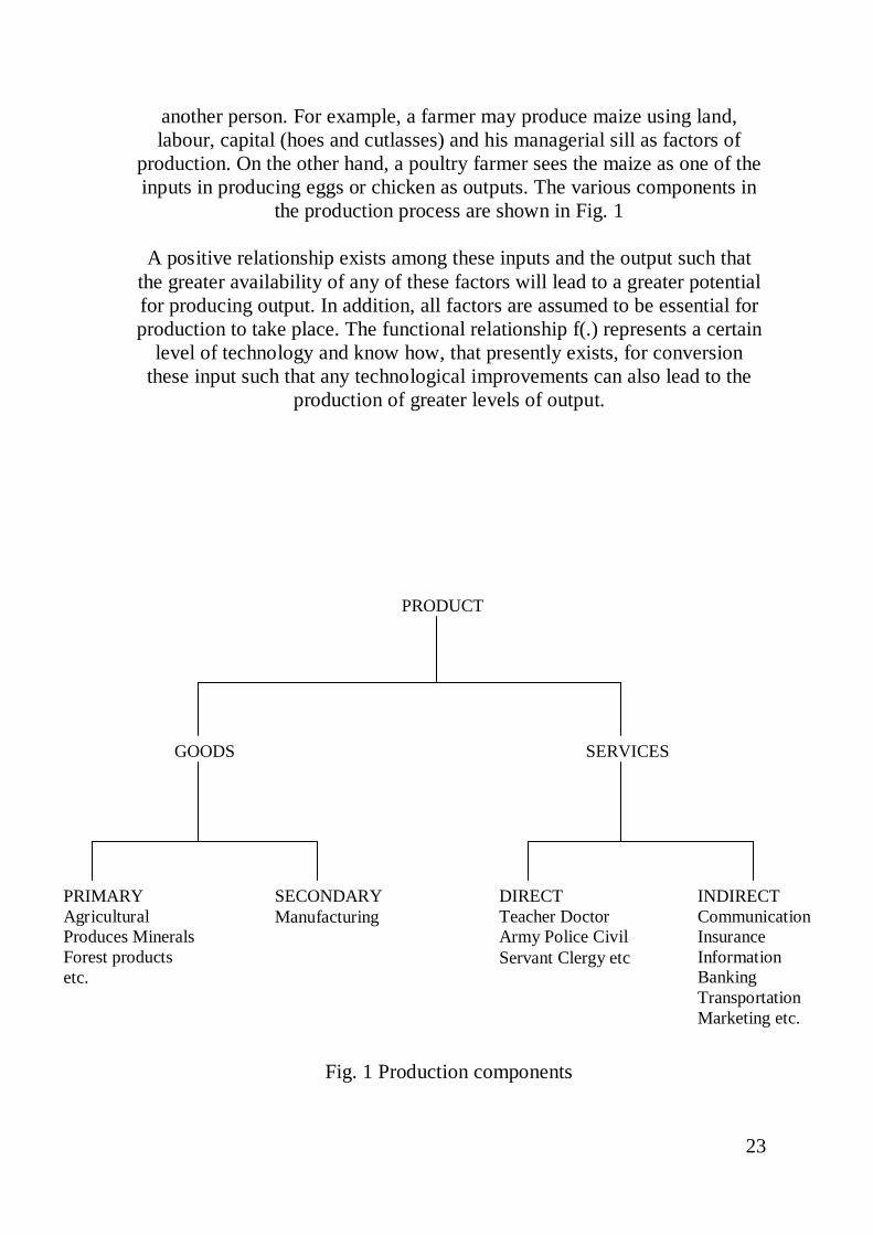
production. On the other hand, a poultry farmer sees the maize as one of the inputs in producing eggs or chicken as outputs. The various components in

the production process are shown in Fig. 1

A positive relationship exists among these inputs and the output such that the greater availability of any of these factors will lead to a greater potential for producing output. In addition, all factors are assumed to be essential for production to take place. The functional relationship f(.) represents a certain

level of technology and know how, that presently exists, for conversion these input such that any technological improvements can also lead to the

production of greater levels of output.

Fig. 1 Production components

PRODUCT

GOODS SERVICES

PRIMARY Agricultural Produces Minerals Forest products etc.

SECONDARY Manufacturing

DIRECT Teacher Doctor Army Police Civil Servant Clergy etc

INDIRECT Communication Insurance Information Banking Transportation Marketing etc.

24

Egg production process requires at least two inputs, feeds and pullets in addition to other fixed input like water, housing etc .in every case,

production can only take place with at least two inputs.

3.2 Factors of Production A factor of production can be defined as that good and service which is

required for production. A factor is indispensable for production because without it no production will be possible. The factors can be grouped

broadly into four categories though the line of demarcation between some of them is not very clear.

3.2.1 Natural Resources

This includes land, water, climate and soil conditions. These are necessary for agricultural production and without them agriculture is impossible. Land is obviously the most important natural resources for agricultural purposes and is often defined economically to include all materials and forces that

supplied by nature for use in the production of goods and services. In other words, land include all the other natural resources e.g. water, forest, soil,

climate, etc

3.2.2 Labour Labour can defined as all human efforts made in the process of transforming inputs to output. Labour is always used in combination with other factors to

produce outputs. The labour may be skilled or unskilled, family, hired or exchange. Labour is measured agriculturally per day, i.e., Man-day. For

accounting purposes, children labour is rated 0.5 unit of adult while woman and old men (over 60 years) are rated 0.75 units of adult. But this practice

may not be totally acceptable in today’s situation.

3.2.3 Capital Capital can be called produced means of production or intermediate

Production. It represents resources produced by past human efforts. Capitals include long-term investment seen as buildings, machinery as well as equipment, implements such as tractors and their implements. Seeds,

fertilizers, as well as cash (at hand) are all capital. Capital may also include tree crops, breeding stock (of animals), dairy cattle, and bullocks (used in land preparation) as well as bullock plough. Some capital normally loss

value with years, the annual loss in momentary term is called depreciation or capital term called appreciation or capital gain or accumulation.

3.2.4 Management or Entrepreneurship

This is a qualitative input as against others, which are quantitative. It is the effective harnessing of the other factors of production for maximum profit.

25

Thus it involves planning, decision-making, supervision, evaluation and general co-ordination of all activities on the farm.

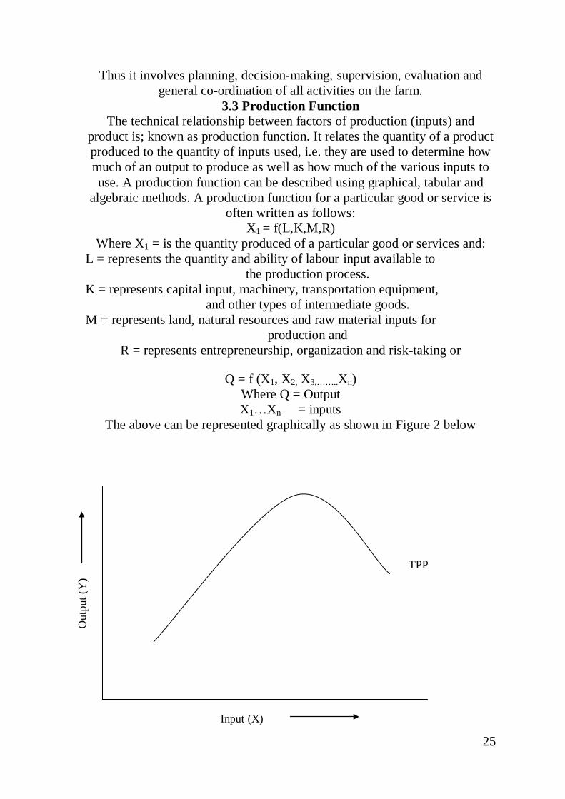
3.3 Production Function The technical relationship between factors of production (inputs) and

product is; known as production function. It relates the quantity of a product produced to the quantity of inputs used, i.e. they are used to determine how much of an output to produce as well as how much of the various inputs to use. A production function can be described using graphical, tabular and

algebraic methods. A production function for a particular good or service is often written as follows:

X1 = f(L,K,M,R) Where X1 = is the quantity produced of a particular good or services and:

L = represents the quantity and ability of labour input available to the production process.

K = represents capital input, machinery, transportation equipment, and other types of intermediate goods.

M = represents land, natural resources and raw material inputs for production and

R = represents entrepreneurship, organization and risk-taking or

Q = f (X1, X2, X3,……..Xn) Where Q = Output X1…Xn = inputs

The above can be represented graphically as shown in Figure 2 below

Out

put (

Y)

TPP

Input (X)

26

Fig. 2: Production Function

The production function can be studied under two situations i.e. short term and long term. Under the short run production function, it is assumed that at

least one input is fixed and hence there are three possibilities.

When only one product is produced, and only one output is variable. This is known as one factor, one product relationship. It determines the most

profitable amount of input to use. When one product is produced but two inputs are variable factors i.e. tow

factor- one product (factor-factor) relationship. It determines the best combination of inputs to use.

When one variable factor is used to produce two products, i.e., one factor-two products (product-product), relationship. It determines right

combination of various products. When many products are produced using as many variable inputs as possible. This is the most realistic especially in Nigeria but the most difficult

to compute and analyse. Its analysis is only possible by use of linear programming.

3.4 Production in the Short and Long run

In this section, we shall be examining both situations when time is so short as to effect any change in the quantity of factors used in the production and a

period long enough for some factors to be variable. 3.4.1 Assumptions under Short-Run and the long –run Functions

There are some assumptions about the production function.

3.4.1.1 Production in the Short Run: in order to better understand the technological nature of production, we distinguish between short run production relationships where only one factor input may vary(typically labour) in quantity holding the other factors of production constant (i.e.,

capital and/or materials)and the long run where all factors of production may vary. The short run allow for the development of a simple two variable

model to understand the behavior between a single variable input and the corresponding level of output. Thus we can write:

X1 = f(L,K,M,R) or X1 =f (L)

For example we could develop a short run model for agricultural production where the output is measures as kilograms of grain and labour is the variable

input. The fixed factor production includes the following:

27

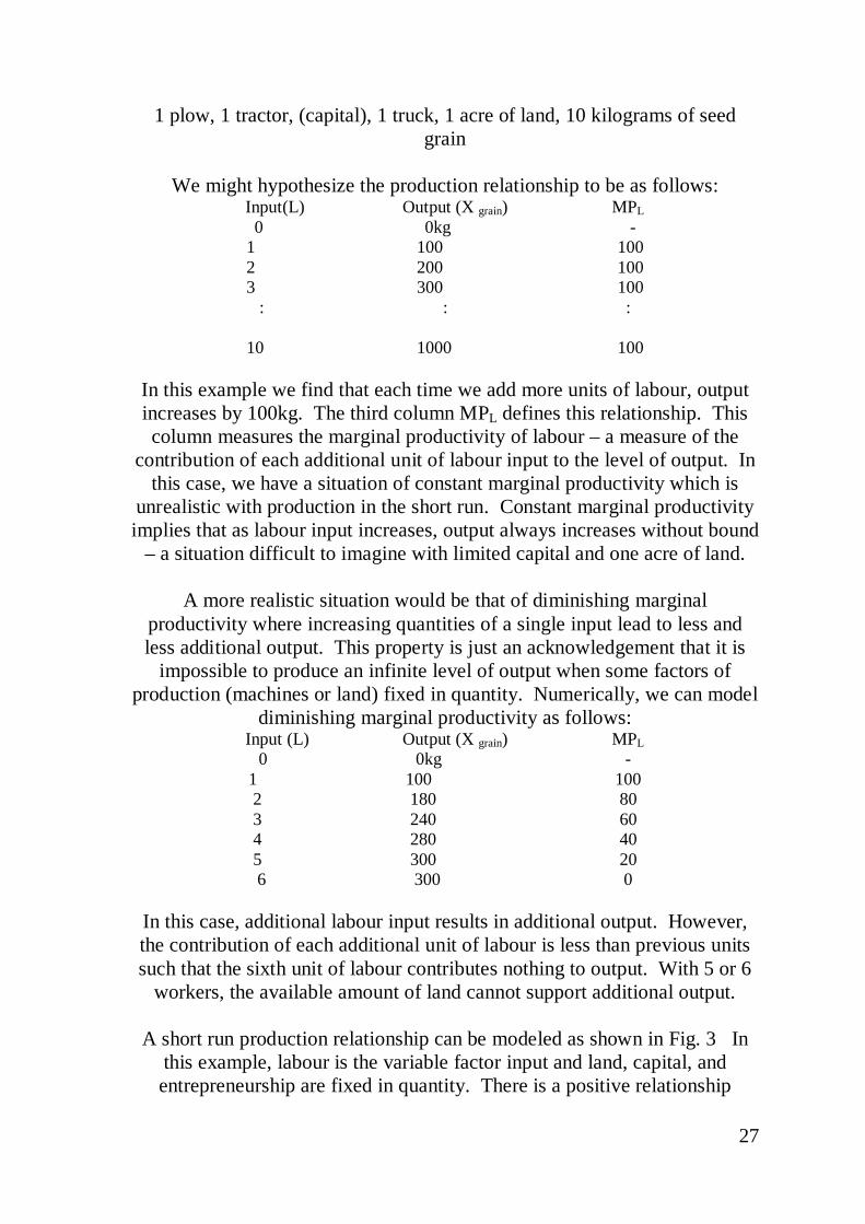
1 plow, 1 tractor, (capital), 1 truck, 1 acre of land, 10 kilograms of seed grain

We might hypothesize the production relationship to be as follows:

Input(L) Output (X grain) MPL 0 0kg -

1 100 100 2 200 100 3 300 100

: : :

10 1000 100

In this example we find that each time we add more units of labour, output increases by 100kg. The third column MPL defines this relationship. This column measures the marginal productivity of labour – a measure of the

contribution of each additional unit of labour input to the level of output. In this case, we have a situation of constant marginal productivity which is

unrealistic with production in the short run. Constant marginal productivity implies that as labour input increases, output always increases without bound

– a situation difficult to imagine with limited capital and one acre of land.

A more realistic situation would be that of diminishing marginal productivity where increasing quantities of a single input lead to less and less additional output. This property is just an acknowledgement that it is

impossible to produce an infinite level of output when some factors of production (machines or land) fixed in quantity. Numerically, we can model

diminishing marginal productivity as follows: Input (L) Output (X grain) MPL

0 0kg - 1 100 100 2 180 80 3 240 60 4 280 40 5 300 20 6 300 0

In this case, additional labour input results in additional output. However, the contribution of each additional unit of labour is less than previous units such that the sixth unit of labour contributes nothing to output. With 5 or 6

workers, the available amount of land cannot support additional output.

A short run production relationship can be modeled as shown in Fig. 3 In this example, labour is the variable factor input and land, capital, and entrepreneurship are fixed in quantity. There is a positive relationship

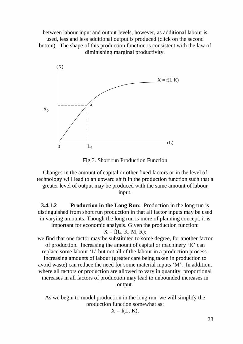
28

between labour input and output levels, however, as additional labour is used, less and less additional output is produced (click on the second

button). The shape of this production function is consistent with the law of diminishing marginal productivity.

Fig 3. Short run Production Function

Changes in the amount of capital or other fixed factors or in the level of technology will lead to an upward shift in the production function such that a

greater level of output may be produced with the same amount of labour input.

3.4.1.2 Production in the Long Run: Production in the long run is

distinguished from short run production in that all factor inputs may be used in varying amounts. Though the long run is more of planning concept, it is

important for economic analysis. Given the production function: X = f(L, K, M, R);

we find that one factor may be substituted to some degree, for another factor of production. Increasing the amount of capital or machinery ‘K’ can

replace some labour ‘L’ but not all of the labour in a production process. Increasing amounts of labour (greater care being taken in production to

avoid waste) can reduce the need for some material inputs ‘M’. In addition, where all factors or production are allowed to vary in quantity, proportional

increases in all factors of production may lead to unbounded increases in output.

As we begin to model production in the long run, we will simplify the

production function somewhat as: X = f(L, K),

X = f(L,K)

X0 a

0 L0 (L)

(X)

29

where we assume that the extraction of raw materials or the development of land is accomplished with combinations of labour and capital input.

Entrepreneurship is embedded in the production technology used [f(.)]. This allows for a two-dimensional representation of combinations of factor inputs

required to produce chosen levels of output. It is possible to produce 100 units of output (X = 100) with the following

combinations of labour and capital. L K

50 200 – Capital Intensive Production 100 100 – Equal Amounts

200 50 -- Labour Intensive Production

4.0 Conclusion If the production technology allows, we could double the quantity of each

input and perhaps double the amount of output. These points represent capital and labour combinations that allow for this greater level of output.

By tripling the original quantity of inputs might allow for a tripling of output. For a given production technology it is not possible to say that using

one factor more intensively than the other is better or more efficient. In economies where capital is relatively scarce and therefore relative more expensive in use as compared to labour, a labour intensive production

process may be more efficient. If the opposite is true (labour being relatively scarce), then capital intensive production may be observed. The

actual combination of factor inputs will depend on their relative productivities and existing factor prices.

5.0 Summary

In this unit, we have studied production, production function, factors of production and production in the Short-run and long-run. While all factors are assumed to be fixed in the short run, they become variable in the long run. Many analyses take the long run concept into consideration for policy making this because it allows adjustments in the nature of inputs such that

all inputs are variable in the long run.

6.0 Tutor-marked Assignment 1. Define Production, and explain capital as a factor of production.

2. Formulate a production function for two variable inputs and three fixed inputs.

3. Why is entrepreneurship so important in production?


30

1. Adegeye, A.J and J.S. Dittoh (1982): Essentials of Agricultural Economics. Centre for Agriculture and Rural Development (CARD)

University of Ibadan, Ibadan. 2. Jhingan, M.L (2006). Microeconomic Theory. Vrinda Publications

Ltd. Delhi. 3. Koutsoyiannis, A. (1984). Modern Microeconomics. Macmillan

Publishers. London. 4. Samuelson, P.A. Economics. Mcmillan, London

31

UNIT 2 PRINCIPLES AND CONCEPTS IN PRODUCTION ANALYSIS


3.0 Main Body 3.1 Law of Diminishing Marginal return 3.2 Principle of maximum Profit

3.3 Principles of Limited Resources 3.4 Physical Product

3.4.1 Total Physical Product 3.4.2 Average Physical Product 3.4.3 Marginal Physical Product

3.5 Elasticity of Production 3.6.1 Total Value Product

3.6.2 Average Value Product 3.6.3 Marginal Value Product

3.6.4 Total Factor Cost 3.6.5 Average Factor Cost 3.6.6 Marginal Factor Cost

3.7 Comparative Advantage 3.8 Gross Margin and farm profit



1.0 Introduction

To get a good grasp of production, some terms and principles must be defined.

2.0 Objective

It is expected that at the end of this unit, you should be able to: -Master some definitions as they relate to the principles of production.

-Apply these learnt principles to practical situations.

Main body PRINCIPLES AND TERMS

3.1 Law of Diminishing Marginal Returns The law states that as a variable input are added to a fixed input(s), added

output increases at a decreasing rate, after initial increasing marginal returns. This is clearly illustrated by the generalized production functions.

3.2 Principles of Maximum Profit

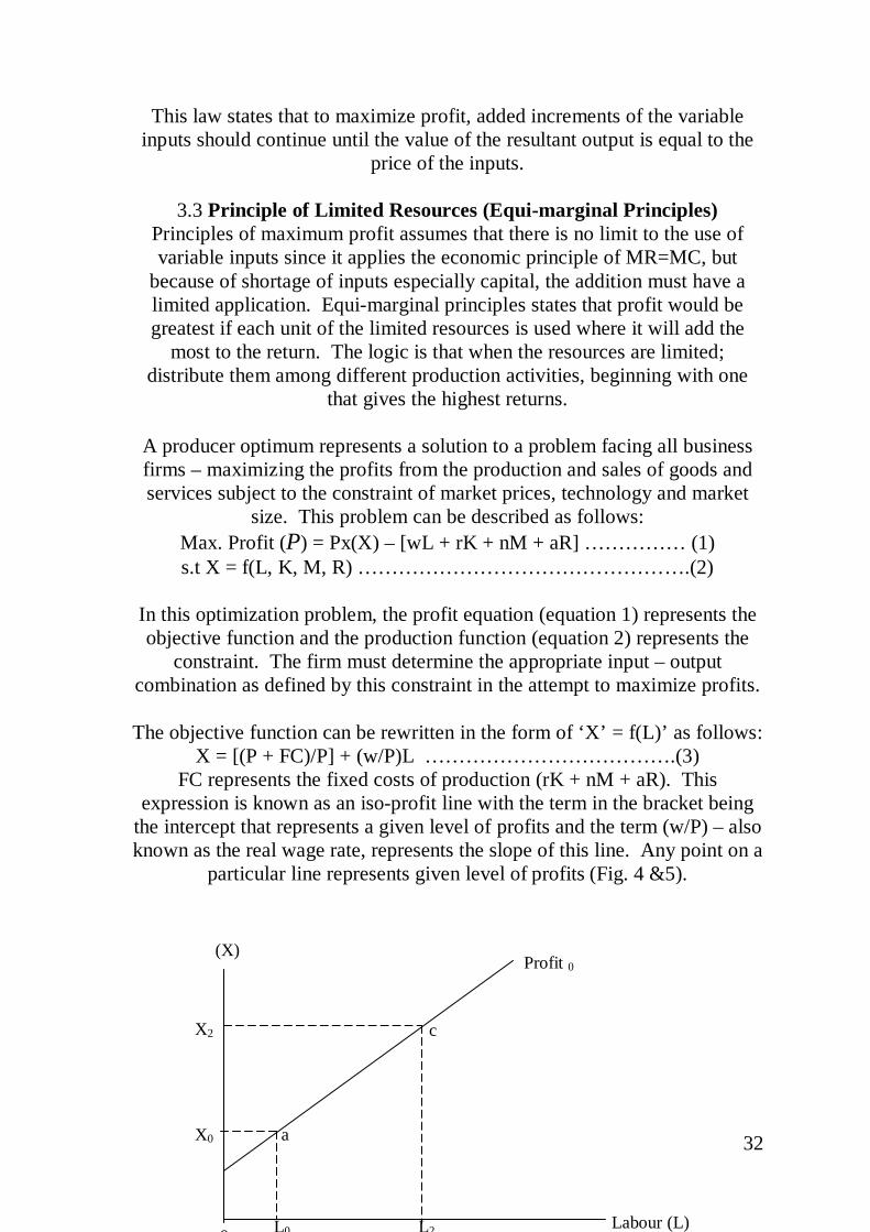
32

This law states that to maximize profit, added increments of the variable inputs should continue until the value of the resultant output is equal to the

price of the inputs.

3.3 Principle of Limited Resources (Equi-marginal Principles) Principles of maximum profit assumes that there is no limit to the use of variable inputs since it applies the economic principle of MR=MC, but

because of shortage of inputs especially capital, the addition must have a limited application. Equi-marginal principles states that profit would be greatest if each unit of the limited resources is used where it will add the

most to the return. The logic is that when the resources are limited; distribute them among different production activities, beginning with one

that gives the highest returns.

A producer optimum represents a solution to a problem facing all business firms – maximizing the profits from the production and sales of goods and services subject to the constraint of market prices, technology and market

size. This problem can be described as follows: Max. Profit (P) = Px(X) – [wL + rK + nM + aR] …………… (1) s.t X = f(L, K, M, R) ………………………………………….(2)

In this optimization problem, the profit equation (equation 1) represents the objective function and the production function (equation 2) represents the

constraint. The firm must determine the appropriate input – output combination as defined by this constraint in the attempt to maximize profits.

The objective function can be rewritten in the form of ‘X’ = f(L)’ as follows:

X = [(P + FC)/P] + (w/P)L ……………………………….(3) FC represents the fixed costs of production (rK + nM + aR). This

expression is known as an iso-profit line with the term in the bracket being the intercept that represents a given level of profits and the term (w/P) – also known as the real wage rate, represents the slope of this line. Any point on a

particular line represents given level of profits (Fig. 4 &5).

Profit 0

X0 a

0 L0 Labour (L)

(X)

c

L2

X2

33

Fig 4 : Producer Optimum The combination of Lo, Xo corresponds to a level of profits of po. Likewise the combination of L2 (greater costs) and x2 (more revenue) also corresponds

to this same level of profits (po) – revenue and costs increase by the same amount. However, the combination of L1 and X1correspond to a greater level of profits relative to the combination of Lo, Xo (revenue increases

more than costs).

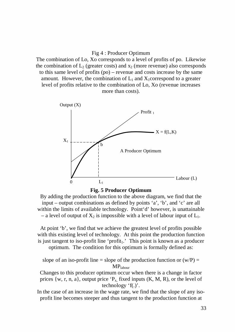
Fig. 5 Producer Optimum By adding the production function to the above diagram, we find that the input – output combinations as defined by points ‘a’, ‘b’, and ‘c’ are all

within the limits of available technology. Point‘d’ however, is unattainable – a level of output of X2 is impossible with a level of labour input of L1.

At point ‘b’, we find that we achieve the greatest level of profits possible

with this existing level of technology. At this point the production function is just tangent to iso-profit line ‘profit1.’ This point is known as a producer

optimum. The condition for this optimum is formally defined as:

slope of an iso-profit line = slope of the production function or (w/P) = MPlabour

Changes to this producer optimum occur when there is a change in factor prices {w, r, n, a}, output price ‘Px, fixed inputs (K, M, R), or the level of

technology ‘f(.)’. In the case of an increase in the wage rate, we find that the slope of any iso-

profit line becomes steeper and thus tangent to the production function at

X = f(L,K)

X1 b

0 L1 Labour (L)

Output (X)

A Producer Optimum

Profit 1

34

some point to the left of the original. At this new producer optimum, we find that the firm will react by hiring less labour now that this input is more expensive, and as a consequence reduces the level of output produced. In

this example, revenue falls, and the costs of production increase (less labour but at a higher wage rate). The profits of the firm will be reduced.

The objective of resources management is therefore: Increase output with the same level of input Get the same level of output with less input Get more output with relatively less input

3.4 Physical Product

3.4.1 Total Physical Product (TPP): This is the quantity of the output measured in physical terms e.g. bags,

mudus, kilograms, baskets, liters, etc.

3.4.1 Average Physical Product (APP): This is the quantity of output per unit of the variable inputs used in its

production. It is sometimes called efficiency of the variable input(s). All lines from the origin intersecting the TPP give the APP at that point of

intersection. APP is calculated thus APPX i = TPP/

APP is measured in respect of each variable input. 3.4.3 Marginal Physical Product (MPP):

This is the addition to TPP as a result of a unit increase in the use of the variable input and it is the slope of the TPP and can be measured at any

point on the TPP curve. It can be calculated thus: MPPX I = ΔTPP/ ΔXi

MPP is measured in terms of each variable input.

3.5 Elasticity of Production (Ep): This measures the response of the output (Q1) to changes in the variable

input. It is calculated thus:

___Ep = percentage change in variable input

percentage change in output__

[ΔQ(Q-1)]/[ΔX/X-1]

= ΔQ X X = ΔQQ ΔX ΔX Q

X X

but APP = Q and MPP = Q X ΔX

Δ Q

35

: . Ep = APP

MPP

If Ep = 1, then there is constant returns to scale, if Ep > 1 then there is increasing returns to scale while if Ep < 1 then there is decreasing returns to

scale. 3.6.1 Total Value Product (TVP)

This is the monetary value of the total output obtained in a production process. It is given as TVP = TPP x P.

3.6.2 Average Value Product (AVP)

This is the average return obtained in a production process. It is obtained as

TVP = AVPx = APPx .PQ = X1 X1 . PQ

TPP

AVP is return per unit of each variable input.

3.6.3 Marginal Value Product (MVP) It is addition to total value product by using one more unit of a variable

input. It is obtained as

ΔTVP = MVPx = MPPx .PQ = X1 X1 .PQ

ΔTPP

Stated in another way, it is the value of additional output resulting from the

use of additional input.

3.6.4 Total Factor Cost (TFC) This is the total money cost of the factors used in a production process. It is

obtained as

TFC = ∑X1 .Px

3.6.5 Average Factor Cost (AFC) This is the average cost of the factors or cost per unit of the factors in a

production process. It is given as

AFC = Xi TFC

3.6.6 Marginal Factor Cost (MFC): This is addition to total costs by using an extra unit of the variable input. It

is given as

ΔTFC MFC = ΔX1 = ΔX1

Δ(∑{X1 .Px })

36

In all the above definitions:

Xi = Variable input(s) Qi = Output(s)

Pxi = Price of input(s) PQ = Price of output(s)

3.7 Comparative advantage The concept of comparative advantage simply is specialization of countries

or regions in production of goods in which it has comparative advantage and imports those in which it has comparative disadvantage. In agriculture, the concept is very important because weather and soil conditions vary from

place to place. If for instance, it costs country A N30 to produce a kilogramme crop X and N40 to produce crop Y wile it costs country B N50 to produce a kilogramme crop X and N30 to produce crop y country A has advantage in producing crop X while country B has advantage in producing

crop Y. The principle encourages country A to concentrate in the production of X while country B concentrates on Y and they in turn imports the other

crop for which they are at disadvantage. A farm firm should produce or engage in enterprises in which it has comparative advantage e.g. in

producing cattle, savannah, and region has comparative advantage over the other areas of country because: i) There is vast grassland

ii) Cattle move freely over a long distance without obstruction iii) There is adequate water supply

iv) There is less tsetse fly infestation, and v) The climate is favourable.

3.8 Gross Margin and Farm Profit

Gross margin of an enterprise is the difference between total value of products and the variable costs of production. The gross margin of an

enterprise measures the contribution of that enterprise to the farm’s total profit given the fixed costs on a farm, the larger the total gross margin from all enterprises on the farm, the larger the profit. When the gross margins for each enterprise has been decided, they are all added together and from this,

the fixed cost (common costs) are deducted. What is left is farm profit? Gross margin = value of gross output - variable costs for each enterprise

combination i.e. GM1 = VGO1– VC1 for enterprise ‘i’

Where VGO = Q.PQ VC = X.Px

It is mostly used in cases where the fixed cost is negligible as in peasant farming.

37

4.0 Conclusion Knowing the definition of Production is not enough but in addition,some

basic practical principles which enable you to apply the knowledge gained to real life issues. The producer is not only interested in total product but average and marginal issues. The students have been exposed to these.

5.0 Summary

Entrepreneurs have to use the concepts of average and marginal issues in order to determine the comparative advantages available to him for his

production decision making process.

6.0 Tutor-marked Assignment 1. What is the relationship between APP, MPP and TPP?

2. Explain the concept of Elasticity of Production and its importance for the Decision maker.

3. Explain the concept of comparative advantage and its application to Nigeria.

7.0 References/Further readings 1. Adegeye, A.J and J.S. Dittoh (1982): Essentials of Agricultural Economics.

Centre for Agriculture and Rural Development (CARD) University of Ibadan, Ibadan.



4. Samuelson, P.A. Economics. Mcmillan, London

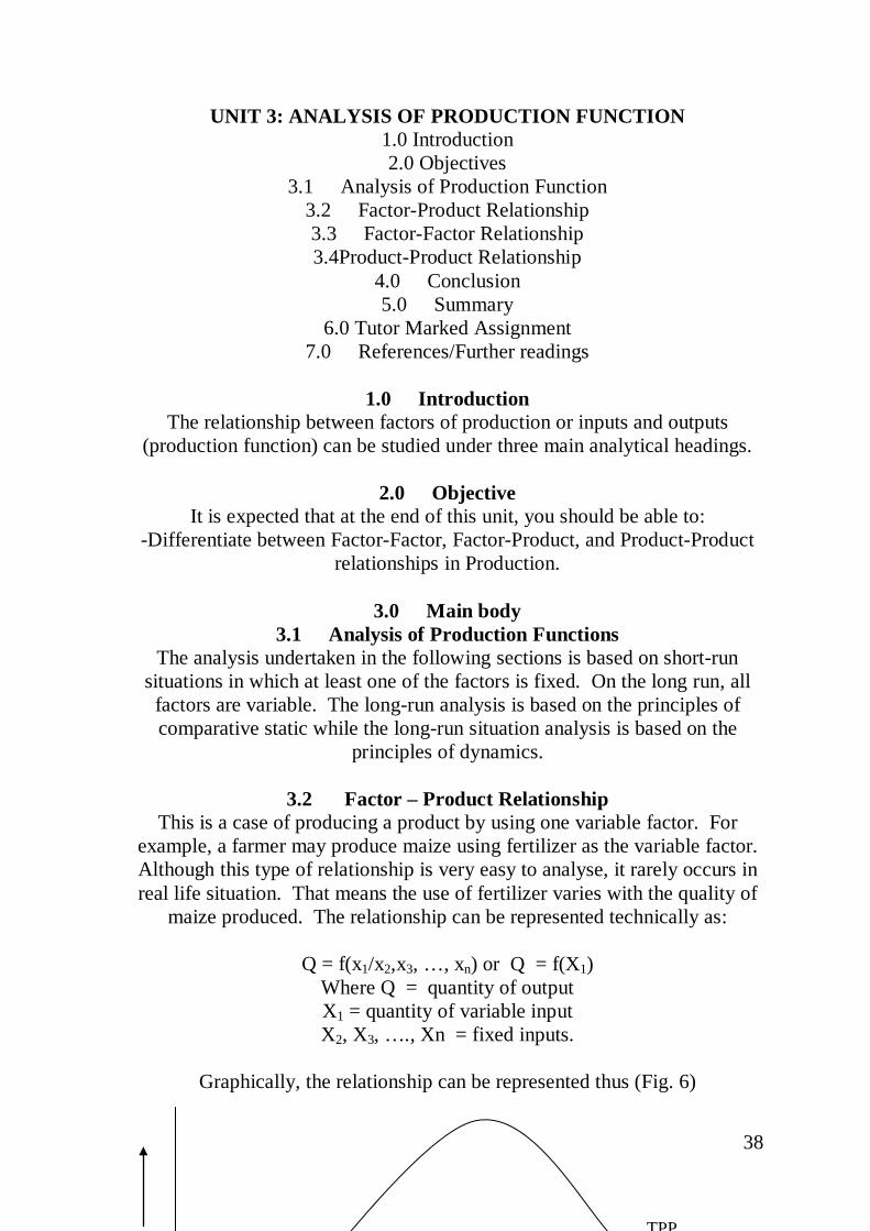
38

UNIT 3: ANALYSIS OF PRODUCTION FUNCTION 1.0 Introduction 2.0 Objectives

3.1 Analysis of Production Function 3.2 Factor-Product Relationship 3.3 Factor-Factor Relationship 3.4Product-Product Relationship



1.0 Introduction

The relationship between factors of production or inputs and outputs (production function) can be studied under three main analytical headings.

2.0 Objective

It is expected that at the end of this unit, you should be able to: -Differentiate between Factor-Factor, Factor-Product, and Product-Product

relationships in Production.

3.0 Main body 3.1 Analysis of Production Functions

The analysis undertaken in the following sections is based on short-run situations in which at least one of the factors is fixed. On the long run, all

factors are variable. The long-run analysis is based on the principles of comparative static while the long-run situation analysis is based on the

principles of dynamics.

3.2 Factor – Product Relationship This is a case of producing a product by using one variable factor. For

example, a farmer may produce maize using fertilizer as the variable factor. Although this type of relationship is very easy to analyse, it rarely occurs in real life situation. That means the use of fertilizer varies with the quality of

maize produced. The relationship can be represented technically as:

Q = f(x1/x2,x3, …, xn) or Q = f(X1) Where Q = quantity of output X1 = quantity of variable input X2, X3, …., Xn = fixed inputs.

Graphically, the relationship can be represented thus (Fig. 6)

Out

put (

Y)

TPP

39

Fig 6 factor- Product Relationship

The above graph clearly demonstrates the law of diminishing returns, i.e. as more of the variable input is added to the fixed factors, the quantity of output

increases at a diminishing rate. Therefore, the job of the economist is to determine the point of optimum production. Because of diminishing returns, the above graph can be divided into three portions as in Fig 7, (the so-called stages of production) based on the relationship between TPP, APP and MPP,

thus:

Out

put (

Y)

TPP

Input (X) MPP

APP

Stage I Stage II Stage III

Ep > 1 Ep > 1 Ep > 0

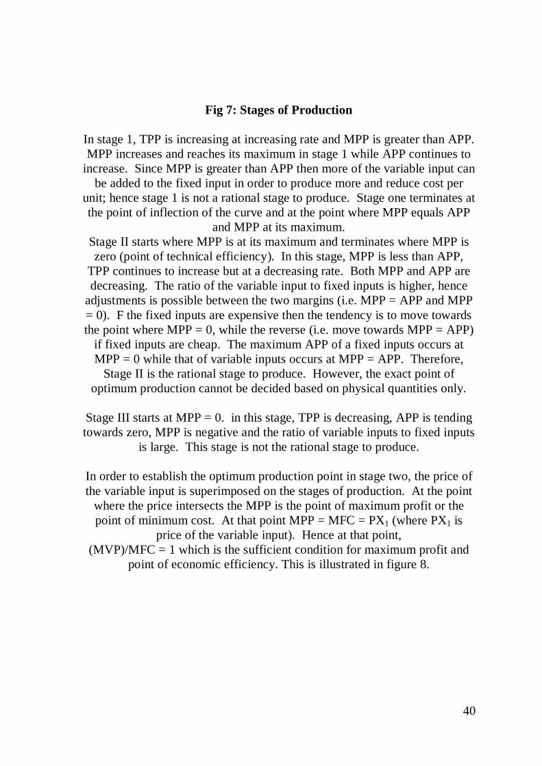
40

Fig 7: Stages of Production

In stage 1, TPP is increasing at increasing rate and MPP is greater than APP. MPP increases and reaches its maximum in stage 1 while APP continues to

increase. Since MPP is greater than APP then more of the variable input can be added to the fixed input in order to produce more and reduce cost per

unit; hence stage 1 is not a rational stage to produce. Stage one terminates at the point of inflection of the curve and at the point where MPP equals APP

and MPP at its maximum. Stage II starts where MPP is at its maximum and terminates where MPP is zero (point of technical efficiency). In this stage, MPP is less than APP,

TPP continues to increase but at a decreasing rate. Both MPP and APP are decreasing. The ratio of the variable input to fixed inputs is higher, hence

adjustments is possible between the two margins (i.e. MPP = APP and MPP = 0). F the fixed inputs are expensive then the tendency is to move towards the point where MPP = 0, while the reverse (i.e. move towards MPP = APP)

if fixed inputs are cheap. The maximum APP of a fixed inputs occurs at MPP = 0 while that of variable inputs occurs at MPP = APP. Therefore,

Stage II is the rational stage to produce. However, the exact point of optimum production cannot be decided based on physical quantities only.

Stage III starts at MPP = 0. in this stage, TPP is decreasing, APP is tending towards zero, MPP is negative and the ratio of variable inputs to fixed inputs

is large. This stage is not the rational stage to produce.

In order to establish the optimum production point in stage two, the price of the variable input is superimposed on the stages of production. At the point

where the price intersects the MPP is the point of maximum profit or the point of minimum cost. At that point MPP = MFC = PX1 (where PX1 is

price of the variable input). Hence at that point, (MVP)/MFC = 1 which is the sufficient condition for maximum profit and

point of economic efficiency. This is illustrated in figure 8.

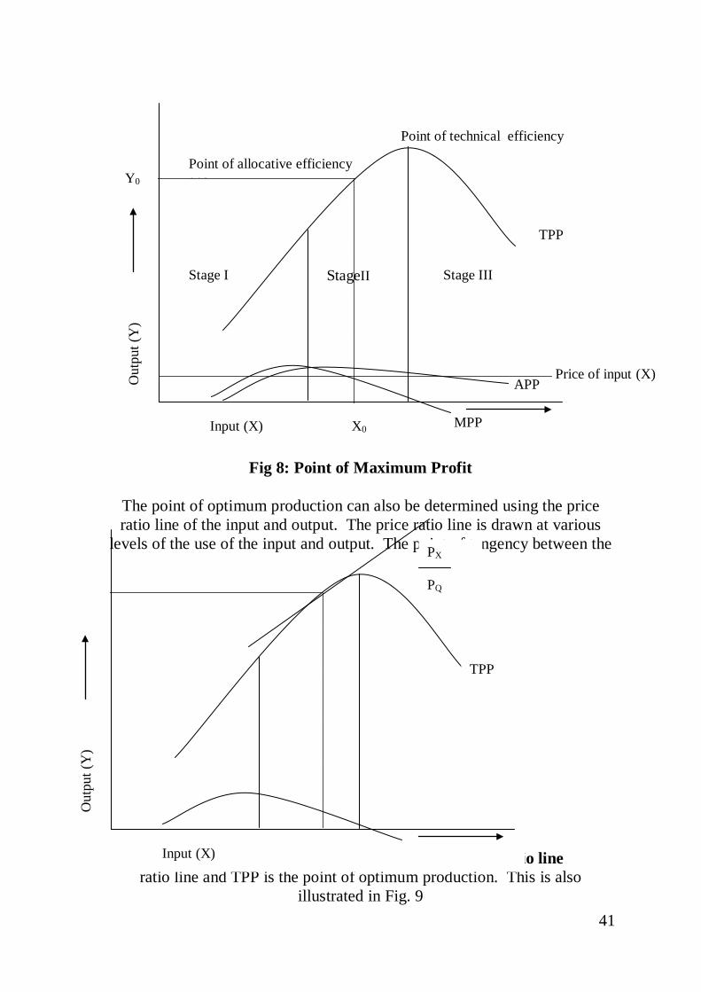
41

Fig 8: Point of Maximum Profit

The point of optimum production can also be determined using the price ratio line of the input and output. The price ratio line is drawn at various

levels of the use of the input and output. The point of tangency between the

Fig 9: Point of Optimum Production using Price ratio line ratio line and TPP is the point of optimum production. This is also

illustrated in Fig. 9

Out

put (

Y)

TPP

Input (X) X0 MPP

APP

Stage I StageII II

Stage III

Point of allocative efficiency ency

Point of technical efficiency

Y0

Price of input (X)

Out

put (

Y)

TPP

Input (X)

PX PQ

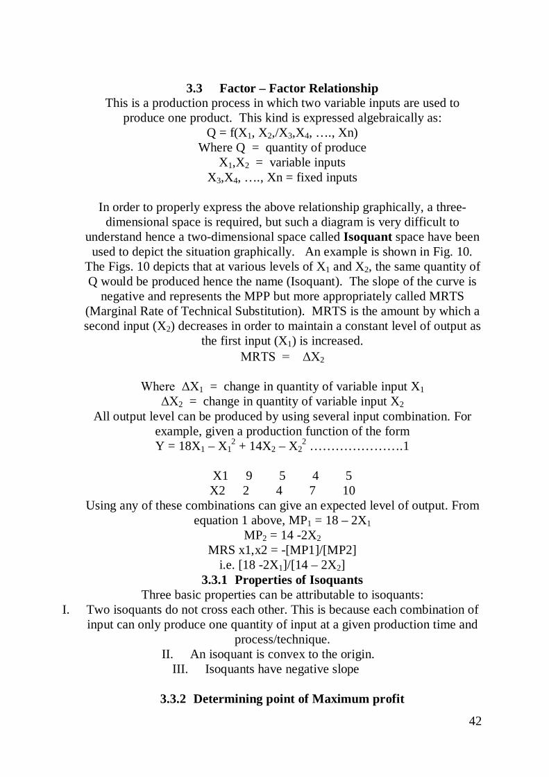
42

3.3 Factor – Factor Relationship

This is a production process in which two variable inputs are used to produce one product. This kind is expressed algebraically as:

Q = f(X1, X2,/X3,X4, …., Xn) Where Q = quantity of produce

X1,X2 = variable inputs X3,X4, …., Xn = fixed inputs

In order to properly express the above relationship graphically, a three-

dimensional space is required, but such a diagram is very difficult to understand hence a two-dimensional space called Isoquant space have been

used to depict the situation graphically. An example is shown in Fig. 10. The Figs. 10 depicts that at various levels of X1 and X2, the same quantity of Q would be produced hence the name (Isoquant). The slope of the curve is

negative and represents the MPP but more appropriately called MRTS (Marginal Rate of Technical Substitution). MRTS is the amount by which a second input (X2) decreases in order to maintain a constant level of output as

the first input (X1) is increased. Δ

MRTS = ΔX2

Where ΔX1 = change in quantity of variable input X1

ΔX2 = change in quantity of variable input X2 All output level can be produced by using several input combination. For

example, given a production function of the form Y = 18X1 – X1

2 + 14X2 – X22 ………………….1

X1 9 5 4 5 X2 2 4 7 10

Using any of these combinations can give an expected level of output. From equation 1 above, MP1 = 18 – 2X1

MP2 = 14 -2X2 MRS x1,x2 = -[MP1]/[MP2]

i.e. [18 -2X1]/[14 – 2X2] 3.3.1 Properties of Isoquants

Three basic properties can be attributable to isoquants: I. Two isoquants do not cross each other. This is because each combination of

input can only produce one quantity of input at a given production time and process/technique.

II. An isoquant is convex to the origin. III. Isoquants have negative slope

3.3.2 Determining point of Maximum profit

43

In order to establish the point of maximum profit, the isocost line is superimposed on the isoquant curve. The isocost line connects all

combinations of two variable inputs, which can be purchased at the same cost. The point of tangency is the point of maximum profit also called line of

least-cost combination (LLCC). The LLCC indicates the point of input combination that gives maximum profit and incurs least cost. Figure 10

illustrates this.

44

Fig 10: Least-cost combination Point

Suppose the farmer is willing to expand the product of Q, all he needs to do is to establish his higher level of production on the isoquant space; and a series of Isoquant lines on one graph give what is called isoquant map.

In order to determine the quantity of output to produce the farmer would simply superimpose the isocost line on each of the isoquants. The line

joining all the LLCC points on the map is called is called expansion path or isocline. Along this isocline, The

Px1

Relationship Px2 = MPPx2 holds true. MPPx1

The sufficient condition for maximum profit along the isocline is the point where MVPx1 = PX1 and MVPx2=Px2….

This implies that the contribution of each input to Q(marginal revenue) must equal price simultaneously (Figure 11).

P1 P2 P3

P3

Q1 Q2 Q3 Q4

Isocost line

Least cost combination point (LCCP)

Isoquant line

45

Fig 11: Expansion Path Connecting the various LLCC

3.4 Product –Product Relationship This is the process in which two products are produced by using one variable input. This process is also called enterprise combination. The relationship is

often represented mathematically as: (Q1,Q2) = f (X1/X2, X3, …..,Xn) or

X1 =f(Q1,Q2) Where X1= variable inputs

X2,X3,…..,Xn =fixed inputs Q1, Q2= products.

Again we would have required a three-dimensional space to represent the

above relationship graphically, but it is instead represented in a two-dimensional space known as production possibility curve (PPC) as shown in

figure 12.

X2

X1

Expansion path

Q2

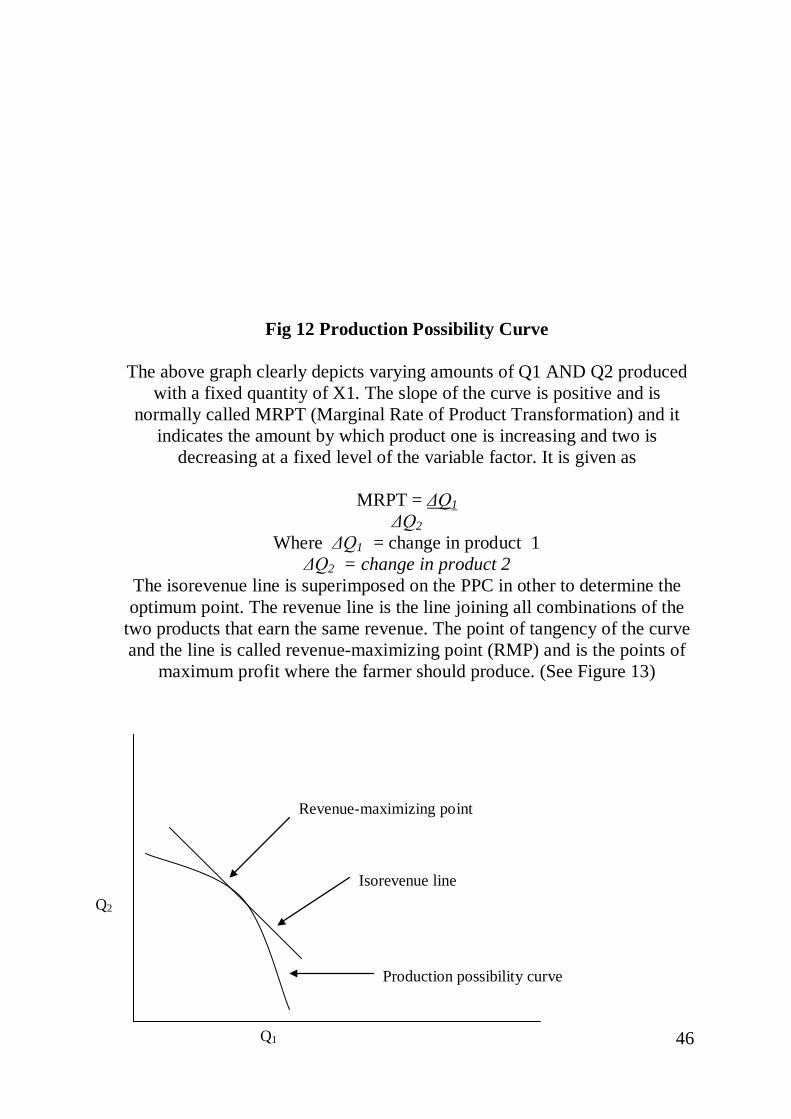
46

Fig 12 Production Possibility Curve

The above graph clearly depicts varying amounts of Q1 AND Q2 produced with a fixed quantity of X1. The slope of the curve is positive and is

normally called MRPT (Marginal Rate of Product Transformation) and it indicates the amount by which product one is increasing and two is

decreasing at a fixed level of the variable factor. It is given as

MRPT = ΔQ2

ΔQ1

Where ΔQ1 = change in product 1 ΔQ2 = change in product 2

The isorevenue line is superimposed on the PPC in other to determine the optimum point. The revenue line is the line joining all combinations of the

two products that earn the same revenue. The point of tangency of the curve and the line is called revenue-maximizing point (RMP) and is the points of

maximum profit where the farmer should produce. (See Figure 13)

Q2

Q1

Revenue-maximizing point

Isorevenue line

Production possibility curve

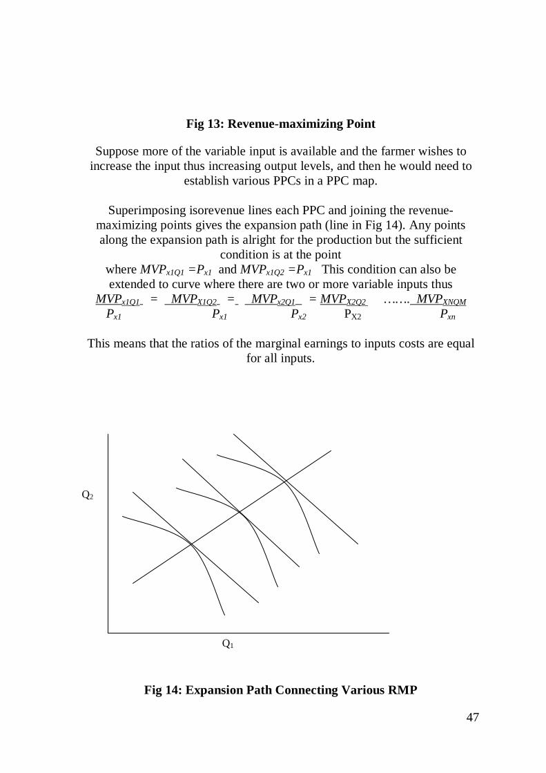
47

Fig 13: Revenue-maximizing Point

Suppose more of the variable input is available and the farmer wishes to increase the input thus increasing output levels, and then he would need to

establish various PPCs in a PPC map.

Superimposing isorevenue lines each PPC and joining the revenue-maximizing points gives the expansion path (line in Fig 14). Any points along the expansion path is alright for the production but the sufficient

condition is at the point where MVPx1Q1 =Px1 and MVPx1Q2 =Px1 This condition can also be extended to curve where there are two or more variable inputs thus

MVPx1Q1 = MVPX1Q2 = MVPx2Q1 = MVPX2Q2 …….Px1 Px1 Px2 PX2 Pxn

MVPXNQM

This means that the ratios of the marginal earnings to inputs costs are equal

for all inputs.

Fig 14: Expansion Path Connecting Various RMP

Q2

Q1

48

4.0 Conclusion

There are three stages in the production process. The stage of rational production is the stage II. However, the point of production which

maximizes the producer’s objective is determined through the imposition of price variable into the model. The producer could thus produce to either

maximise revenue, profit or minimize costs. This is achieved at the point of tangency between the isoquant and the isocost line. For the revenue

maximization, the iso-revenue line must be tangent to the production possibility curve.

5.0 Summary In this unit, we have differentiated between the three relationships in

production. These could be factor-factor, factor-product or product-product relationships. There are three stages in the production process namely: stage

I, stage II and Stage III. While it pays the producer to keep increasing the quantity of variable inputs used in this stage, the reverse is the case in stage

III. Stage II is the stage of rational production.

6.0 Tutor-marked Assignment Determine the Optimum profit point in a factor-factor and factor-product

relationship.




3.Koutsoyiannis, A. (1984). Modern Microeconomics. Macmillan Publishers. London.

4. Samuelson, P.A. Economics. Mcmillan, London

49

UNIT 4: RELATIONSHIPS AMONG INPUTS AND PRODUCTS 1.0 Introduction 2.0 Objectives

3.1 Relationship between Inputs 3.2 Relationships between Outputs



7.0 Introduction

Form the previous unit, you were told that inputs and outputs do substitute one for another. Thus there is a type of relationship existing between these two i.e. inputs and output/products on the farm. The need to realize this is seen in the fact that knowledge of this relationship will help the decision

maker or farm manager know how the inputs are used and how the products are produced in proportions to help in resource allocation and utilization.

8.0 Objectives

At the end of this unit, you are expected to be: a. Able to determine the type of relation existing between inputs and outputs

during the production process. b. Advice on resource allocation for any type of relationship between either

inputs or products.

3.1 Relationships between Inputs Inputs are technical substitutes such that it is possible for an increase in one input to lead to a decrease in the other input while maintaining the level of output. They tend to compete with each other though. The marginal rate of technical substitution for these inputs is negative. There are three types of

substitution basically. a. Decreasing rate of substitution b. Constant rate of substitution

c. Increasing rate of substitution Let us look at each of these types of substitution rates.

3.1.1 Constant rate of substitution

This occurs when the amount of input replaced by another input remain unchanged with the addition of the other input. In other words, the isoquant remains unchanged with the change in the input combination. This type of

input are called constant substitutes.

3.1.2 Increasing rate of substitution

50

This is a situation when an increase in an input replaces larger amount of input being substituted. Again we can say that the marginal rate of

substituting input X1 for x2 increases as x1 is increased along the isoquant.

3.1.3 Decreasing Rate of Substitution This occurs when the input being increased substitute for successively

smaller amount of the input being replaced. This is caused mainly by the law of Diminishing returns. This implies that the rate at which X1 substitutes for

X2 decreases as X1 is increased along the isoquant curve.

3.2 Relationships between Products The Production Possibility Curve (PPC) as discussed in Unit 3 helps to

illustrate the relationship which could exist between products on the farm among enterprises. Products or enterprises compete for limited resources such as land, labour, capital and others. For cocoa and oil palm could be

competing for labour use on the farm. The decision maker must ensure that the resources are allocated among these products lines in a manner that the

goal of the firm is achieved. There are four types of relationships which are likely among enterprises or products name: Competitive, complementary,

supplementary and joint relationships.

3.2.1 Competitive Products Products or enterprises are competitive when in the use of resources on the

farm, when output can only be increased through the reduction in the products of the other enterprise. Such products substitute for each other at

an increasing rate. At times they can substitute for each other at a decreasing or constant rate. Price, as have been said in Module One will determine

which one to produce. Two varieties of a crop can substitute at a constant rate. In that case on a parcel of land (limited resource), the ratio of reduction

in land for the production of one variety to an increase in land for the production of the other variety of the same crop can substitute at constant rate. What the farm manager does in such situation is to produce the one

which commands higher price.

3.2.2 Complementary Products Complementarity of products exists when an increase in the production of one product through the transfer of more resource to its production leads to increase in the production of the other product. This occurs more when one

of the products supplies input(s) to the production of the other. For example, production of legumes in crop rotation increases the nitrogen level in the soil for the use of other crops. The legumes have nitrogen fixing bacteria in their

root system (nodules) which fix nitrogen in the soil thus increase the available nitrogen in the soil. Therefore any additional resource committed

51

to cultivating legumes can result in higher grain production in a legume/cereal mixture or in a legume followed by cereal rotation regime.

This advantage could be explored to some level on the farm as the products could soon become competitive with time.

3.2.3 Supplementary Products

This type of relationship exits when the amount of one product can be increased without any effect on the other products. In other word, they are

independent of one another. To produce cocoa and oil palm using labour and some implement can be said to be complementary. The use of pressing

machine for extracting oil does not affect the production of cocoa as it is not needed in cocoa production. Like in the complementary situation, this could also become competitive at some time in the production process. There are

situations when this type of relationship could be taken advantage of.

3.2.4 Joint Products This is a situation when products results from the same production process. The production of one implies the production of the other. They are atimes produced in some ratios. The production of palm oil and palm kernel for

example is together as the same resources: land and oil palm tree are involved. There are some varieties of the palm oil which produce more

palm oil than kernel. So the farmer could take the advantage of this type of scenario in deciding on what to produce. When the demand for palm oil for example is on the increase and price is increasing, the farmer can decide to

go for the variety which yields more palm oil. Switching from variety however, may take time.

9.0 Conclusion

Farmers can take advantage of the type of relationship between inputs and enterprises on the farm to achieve organizational goal. Prices can be

determinant for the type of input to use especially when the substitute for one another in a constant manner.

10.0 Summary

In this Unit, you have learnt that there are four types of relationships possible between inputs during the production process. These are:

Decreasing rate of substitution, Constant rate of substitution, and increasing rate of substitution. On the other hand for the products, you were also told that products can have any of Competitive, complementary, supplementary or joint relationships. Decision maker therefore needs to take advantage of

these relationships in achieving set goal of production.


52

i. Explain the types of relationship which can exist between inputs on a specified enterprise type.

ii. What disadvantage(s) are there in competitive and joint production?





4. Nmadu, J.N and T.T. Amos 2003. An Introduction to Agricultural Economics. Yekabo Educational publishers. P.172.

53

MODULE 3: THEORY OF COSTS AND REVENUE UNIT 1: THEORY OF COSTS


3.0 Main Body 3.1.1 Costs

3.1.2 Cost Functions 3.2 Types of costs

3.2.1 Total Cost 3.2.2 Average costs 3.2.3 Marginal Cost

3.3 Private versus Social Costs 4.0 Conclusion 5.0 Summary


7.0 Introduction

Firms produce commodities in order to make some profits. In the process of making commodities available, firms incur some costs. These costs go a

long way to determine the profit level of the producer and in turn with the demand, the price of the commodity produced.

8.0 Objective(s)

It is expected that at the end of this unit, you should be able to: -Explain those costs incurred in production

-Differentiate between the different types of costs -Relate the different types of costs to the decision maker’s objective.

3.0 THEORY OF COSTS

3.1.1 Cost Definition Cost refers to the value of inputs used in production. The traditional theory distinguishes two types of costs in terms of the short run and the long run periods. The short run is the period during which some factor(s) is fixed; usually capital equipment and management are considered as fixed in the

short run. The long run is the period over which all factors become variable. Thus the firm’s total cost are split into two groups : total fixed costs and the

total variable costs. These we shall discuss in details shortly. 3.1.2 Cost Function

The cost functions are derived functions. They are derived from the production function, which describes the available efficient methods of

production at any one time. Economic theory always distinguishes between long run and shortrun costs. Thus the cost function is the technical

54

relationship between the quantity of output and the cost of producing the output, e.g.

Q =f(X1) production function

C =f(X1PX1) cost function

The above means the quantity of output is a function of the cost of the variable inputs provided all other factors are fixed. The two functions above

can be represented graphically (in figures 15 A & B) thus:

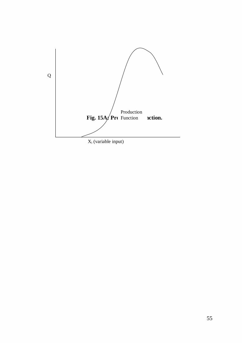
55

Fig. 15A: Production Function.

Q

Xi (variable input)

Production Function

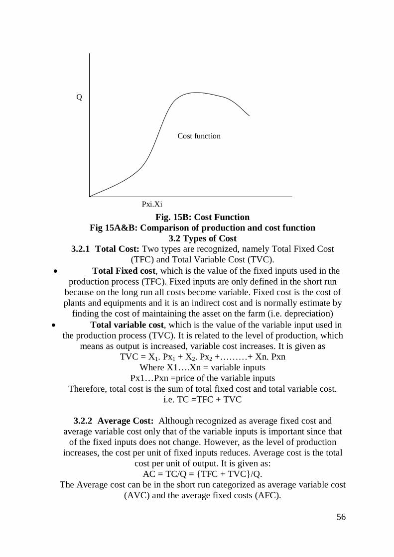
56

Fig. 15B: Cost Function Fig 15A&B: Comparison of production and cost function

3.2 Types of Cost 3.2.1 Total Cost: Two types are recognized, namely Total Fixed Cost

(TFC) and Total Variable Cost (TVC). • Total Fixed cost, which is the value of the fixed inputs used in the

production process (TFC). Fixed inputs are only defined in the short run because on the long run all costs become variable. Fixed cost is the cost of plants and equipments and it is an indirect cost and is normally estimate by

finding the cost of maintaining the asset on the farm (i.e. depreciation) • Total variable cost, which is the value of the variable input used in

the production process (TVC). It is related to the level of production, which means as output is increased, variable cost increases. It is given as

TVC = X1. Px1 + X2. Px2 +………+ Xn. Pxn Where X1….Xn = variable inputs

Px1…Pxn =price of the variable inputs Therefore, total cost is the sum of total fixed cost and total variable cost.

i.e. TC =TFC + TVC

3.2.2 Average Cost: Although recognized as average fixed cost and average variable cost only that of the variable inputs is important since that

of the fixed inputs does not change. However, as the level of production increases, the cost per unit of fixed inputs reduces. Average cost is the total

cost per unit of output. It is given as: AC = TC/Q = {TFC + TVC}/Q.

The Average cost can be in the short run categorized as average variable cost (AVC) and the average fixed costs (AFC).

Q

Pxi.Xi

Cost function

57

AFC = TFC/Q AVC = TVC = X1 P X1 = Px1

Q Q APP 1

The averaged fixed cost is the cost of indirect factors. i.e. the cost of the physical and personal organization of the firm Therefore, average total cost (ATC) is given as ATC =AFC+ AVC. This can be illustrated graphically as

(figure 16):

Fig 16: Average and marginal Costs

3.2.3 Marginal Cost: This is the addition to the cost due to the production of an additional unit of product.

MC = ΔTVC = ΔTFC + ΔTVC but ΔTFC

ΔQ ΔQ ΔQ ΔQ = 0

MC = ΔTVC = ΔX1 P X1 = Px1

ΔQ ΔQ MPP 1

AVC is inversely related to AP while MC is inversely related to MP.

3.3. Private and Social Cost

These terms were first used in the early 1930s. private costs are those costs which firms incurred themselves in the production process. These costs

could be incurred as fixed or variable cost. The production of commodities or services by these firms could lead to some benefits or harm to others. This

is then termed social costs. For example, the production of tobacco by a cigarette firm could lead to the pollution of the environment which leads to

social cost. On the other hand, the production of services like parks and

MC ATC

AVC

MR

AFC

58

schools could lead to social benefits. Adding the private costs of producing units together with the damage others get from the production activities of

these firms e.g environmental pollution; we arrive at the social costs.

4.0 Conclusion The traditional theory of costs recognized the short run and the long run

costs. While the short run is the period so short that costs are fixed. The long run is the period when some cost items become variable. Included in the

former are items such as cost of management and the cost of capital item as building. Costs included in the later category include those for raw materials,

direct labour and running expenses on capital items such as fuel, maintenance costs.

5.0 Summary

The total cost of production can be classified into either fixed or variable. The fixed cost (FC) can be total or average likewise the variable cost (VC). The average variable cost (AVC) is inversely related to the average product

(AP). This is also true for marginal cost and marginal physical product.

6.0 Tutor marked Assignment. 1. Distinguish between fixed and variable cost.

2. Discuss the relationship between Marginal Cost and Marginal Physical Product (MPP).





Publishers. London. 4. Samuelson, P.A. Economics. McMillan, London

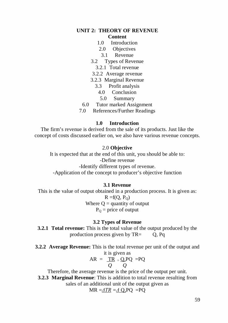
59

UNIT 2: THEORY OF REVENUE Content

1.0 Introduction 2.0 Objectives 3.1 Revenue

3.2 Types of Revenue 3.2.1 Total revenue

3.2.2 Average revenue 3.2.3 Marginal Revenue

3.3 Profit analysis 4.0 Conclusion 5.0 Summary

6.0 Tutor marked Assignment 7.0 References/Further Readings

1.0 Introduction

The firm’s revenue is derived from the sale of its products. Just like the concept of costs discussed earlier on, we also have various revenue concepts.

2.0 Objective

It is expected that at the end of this unit, you should be able to: -Define revenue

-Identify different types of revenue. -Application of the concept to producer’s objective function

3.1 Revenue

This is the value of output obtained in a production process. It is given as: R =f(Q, PQ)

Where Q = quantity of output PQ = price of output

3.2 Types of Revenue

3.2.1 Total revenue: This is the total value of the output produced by the production process given by TR= Q, Pq

3.2.2 Average Revenue: This is the total revenue per unit of the output and

it is given as AR = TR = Q,

Q Q PQ =PQ

Therefore, the average revenue is the price of the output per unit. 3.2.3 Marginal Revenue: This is addition to total revenue resulting from

sales of an additional unit of the output given as MR =ΔTR =Δ Q,PQ =PQ

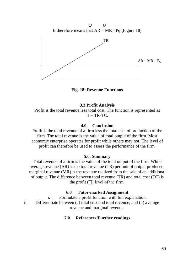
60

Q Q It therefore means that AR = MR =Pq (Figure 18)

Fig. 18: Revenue Functions

3.3 Profit Analysis Profit is the total revenue less total cost. The function is represented as

Π = TR-TC.

4.0. Conclusion Profit is the total revenue of a firm less the total cost of production of the

firm. The total revenue is the value of total output of the firm. Most economic enterprise operates for profit while others may not. The level of

profit can therefore be used to assess the performance of the firm.

5.0. Summary Total revenue of a firm is the value of the total output of the firm. While

average revenue (AR) is the total revenue (TR) per unit of output produced, marginal revenue (MR) is the revenue realized from the sale of an additional of output. The difference between total revenue (TR) and total cost (TC) is

the profit (∏) level of the firm.

6.0 Tutor-marked Assignment i. Formulate a profit function with full explanation.

ii. Differentiate between (a) total cost and total revenue, and (b) average revenue and marginal revenue.


AR = MR = PQ

TR

61




Publishers. London. 4. Samuelson, P.A. Economics. McMillan, London

62

MODULE 4: RESOURCE MANAGEMENT

Unit 1: Nature and Structure of Farm Resources Content


3.0 Nature of Farm Resources 3.1 Renewable Resources

3.2 Non renewable resource 3.3 Demand for Farm Input or Resources

3.4 Valuation of Scare resources 3.4.1 Valuation at cost

3.4.2 Valuation at cost or market price. 3.4.3 Valuation at net selling price.

3.4.4 Valuation at cost less depreciation. 3.4.5 Valuation by reproductive value



3.0 Introduction

In this unit we shall be considering the different farm resources available to the farmer, their nature, type and valuation. This is

needed for planning the allocation of these resources. Planning has to take place because of the innate nature of the resources if the

farmer must achieve set goals.

4.0 Objective i. At the end of this unit, you should be familiar with the nature of farm

resources. ii. The student is expected to be able to classify any resource.

iii. Also, you are expected to be able to value any farm resource.

3.0 Nature of Farm Resources The traditional factors of production are land, labour, capital and

entrepreneur. The major attribute of these resources is the limited nature. These resources must be combined in appropriate manner for production to take place. Time is however required for this transformation process to take place. This period is referred to as the production or transformation period.

Given that economics is briefly the study of how scarce resources are allocated, resource economics is the study of how society allocates scarce

63

natural resource and environmental economics is concerned with the conservation of natural environments and biodiversity. These natural resources are often categorized as either renewable or non-renewable.

3.1 Renewable Resources

A renewable resource must display a significant rate of growth on a relevant economic time scale.

3.2 Non renewable resource

A nonrenewable resource on the other hand does not display significant rate of growth or renewal.

3.3 Demand for Farm Input or Resources

Assuming a perfect competition in the factor market, we can derive the short run demand for farm inputs. Given that the inputs are purchased because of

their contribution to the production process, the demand curves for inputs/resources are thus derived from the production function on the assumption that the goal of the entrepreneur is profit maximization.

Q = f(X1, X2) C = r1X1 + r2X2 + b

Where Q = Output

Xi = inputs 1 & 2 Ri = input ‘i’ price

Ρ = price of output ‘Q’ C = total cost of production involved in producing output ‘Q’

We can derive the lagrangian equation as follows: V = ρf(X1X2) + λ[ΰ – ρf(X1X2) + r1X1 + r2X2 + b]

This can be differentiated with respect to x1, x2 and λ to get equations 1, 2 and 3

δV/δX1 = ρf1 – λρf1 + λr1 …………….1 δV/δX2 = ρf2 – λρf2 + λr2 …………….2

δV/δ λ = ΰ – ρf(X1X2) + r1X1 + r2X2 + b …………….3 λρf1 - ρf1 = λr1 ………………………….4 λρf2 - ρf2 = λr2 …………………………..5

ρf1 = [1/(λ – 1)]r1 i.e. VMP1 ρf2 = [1/ (λ – 1)]r2 i.e. VMP2

Thus VMP1 = Kr1, VMP2 = Kr2 …………..6

Where K = 1/(λ – 1) From equation 6, the demand function for any input depends upon the

particular input’s price, the prices of all other inputs and the price of the

64

product. In that case, it depends upon the product price and this is derived from the demand for the product

3.4 Valuation of Scare resources

There is a constant need for valuation of farm assets and resource at various periods and for various reasons. However, doing this at the end of the

accounting period on a farm shows the true position of the farm at the given time in terms of the worth of the farm. Valuation could be done when the

farm is to be disposed. By valuation, it implies attaching prices farm assets such as building, vehicles, and crops on the field, stored products, stock of animals and raw materials. The method used in valuing an asset affects the

profit and or loss on the farm. It is advisable to stick to one type of valuation during a period to avoid arriving at erroneous figures. There are different

methods of valuing assets on the farm. The method to be adopted is determined by the purpose for which the valuation is meant. Five major

methods shall be discussed herein.

3.4.1 Valuation at cost. In this method, the asset’s actual cost of purchase is used. This is appropriate for such asset as building or equipment which do

not loss value fast. 3.4.2 Valuation at cost or market price. This is more important in valuing

purchased assets. 3.4.3 Valuation at net selling price. This method is also used for assets

which are meant for sale. 3.4.4 Valuation at cost less depreciation. This method is used for such

assets as machinery and breeding livestock. 3.4.5 Valuation by reproductive value otherwise known as replacement cost. It is used for valuing assets in relation to what such asset will cost if it were to be replaced at present price using the current production method.

3.5 Depreciation

Depreciation is closely related to valuation as it helps in determining the actual price of any capital resource on the farm. Depreciation therefore helps in determining values of assets. To understand valuation therefore we must first understand depreciation. It is the spreading of the cost of an asset over

its entire useful life. Thus depreciation represents how much a farmer should set aside annually in order to replace a capital asset.

Rate of depreciation for assets vary from asset to asset. This is mainly a result of the intensity of use, care for the asset and maintenance. Three

common methods exist for depreciating assets. These are the straight line method, the declining balance method, and the sum of year digit method.

You are to read this aspect in the relevant course.

65

4.0 Conclusion The resources on the farm are limited as such, proper management is

necessary for achieving organizational goal. There are different methods for assessing the value of the resources for determining the worth of the

enterprise at any time. 5.0 Summary

The resources on the farm are by nature limited. They can be renewable or nonrenewable. There is need to value the resources for proper determination of the worth of the farm at any time. Closely related to this is depreciation.


i. In an identified enterprise list all the probable resources available and their categorization.

ii. What are the major methods for valuing farm capital resources?

7.0 References/Further Readings i. Heady, E.O and W. Gandler. 1958. Linear Programming methods. Iowa

State University Press Ames, Iowa. ii. Olayemi, J.k and C.E. Onyewaku. 1999. Quantitative methods for Business

Decisions. Department of Agricultural Economics, University of Ibadan, Ibadan.

66

Unit 2: Optimization Techniques 1.0 Introduction

Linear programming (LP) is an optimization tool for managing scarce resources for achieving organizational goal. Linear programming came into prominence in the late 1940s and has since gained wide application in the field of agriculture and non-agricultural production process. It is used by

agricultural economists to solve wide range of farm problems.

This unit will expose you to the basics of linear programming as a management tool. Though many computer software of the linear

programming exist today. There are about 49 packages for solving Linear programming today and many may still be released soon.

2.0 Objectives

This unit is designed to acquaint you with the basics of optimization problems.

It is expected that you will be able to formulate and solve linear programming problems.

3.0 Linear programming

This is an optimization technique which grew out of applied mathematics. It is the simplest and the most common mathematical programming model. It involves a linear function of one or more variables subject to one or more

linear constraints. Linear Programming (LP) is a powerful tool for the analysis of economic problems in agriculture and all phases of business.

3.1 Uses of Linear programming Linear programming is used by agricultural economists to analyze a wide

range of farm problems. These include: i. Specification of optimum organization of resource and enterprises on farm. ii. To specify profit maximizing mixes of commodities produced by marketing

firms. iii. Assessment of cost minimizing method of processing farm products and

providing mixes of farm inputs such as fertilizer and seed. iv. To support feasible and possible farm adjustments processes and

alternatives. v. Provide unique and testable solution into related problems.

a. Components of Linear Programming

There are three main components of a linear programming problem. These are:

67

a. Objective function: it states the aim of the model i.e either for maximization of minimization of the objective.

b. Alternative methods or process specification. There exists several methods by which the objective function may be attained and this enables the choice of from these methods the most efficient method in converting

resources into a given objective function. c. Resource restrictions or limitation of resources. Linear programming

does not exist unless resources are known to be limited. This enables a working with the concept of optimal allocation.

b. Assumption of Linear programming There are some assumptions made about linear programming problems without which it may not provide precise solution to problems at hand.

These assumptions are: i. Additive nature of resources and activities: the total amount of resources

used by several enterprises must be equal to the sum of the resources used by each individual enterprise. This doe not allow interaction in the amount of resources required per unit of output regardless of whether activities are

produced singly or in various proportions. ii. Linearity: Input and output ratios are constant and independent of scale.

They can be added as a series of linear equalities. iii. Divisibility: resources and products are infinitely divisible.

iv. Finiteness: Limited number of alternative activities and resource exist. v. Single-valued expectation: resources supplies, input-output coefficient and

prices are known with accuracy. vi. Non-negativity of assumptions: resources to be used must be positive.

c. Steps in Linear Programming Problems

There are some basic steps in solving Linear programming problem. They are as follows:

a) Formulation of objective and its statement: the objective must be well formulated and stated.

b) Identification and listing of relevant variables. Relevant variables to the linear programming problem to be solved must be identified and well listed.

c) Formulation of available strategies. d) Calculation of possible results e.g. revenue, profit or cost.

e) Decision making. To proceed, the necessary data requirements are made namely: List all possible activities which are to be considered.

Calculate net revenue for each activity Determine resource restrictions and other limitations

Detailing the requirement of the activities.

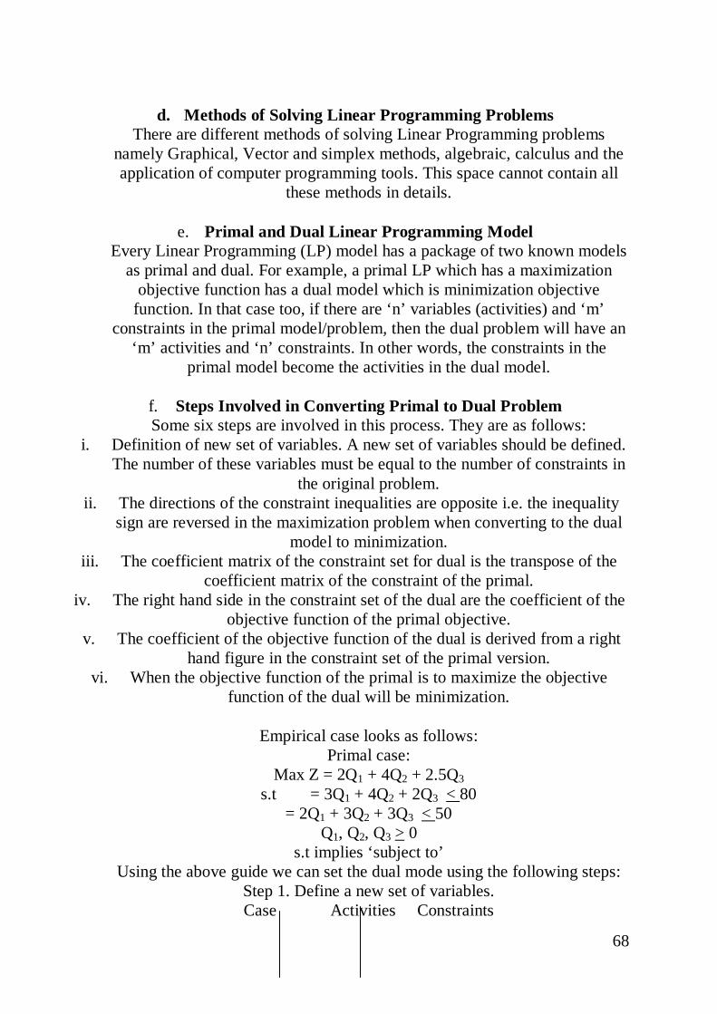
68

d. Methods of Solving Linear Programming Problems

There are different methods of solving Linear Programming problems namely Graphical, Vector and simplex methods, algebraic, calculus and the application of computer programming tools. This space cannot contain all

these methods in details.

e. Primal and Dual Linear Programming Model Every Linear Programming (LP) model has a package of two known models

as primal and dual. For example, a primal LP which has a maximization objective function has a dual model which is minimization objective

function. In that case too, if there are ‘n’ variables (activities) and ‘m’ constraints in the primal model/problem, then the dual problem will have an

‘m’ activities and ‘n’ constraints. In other words, the constraints in the primal model become the activities in the dual model.

f. Steps Involved in Converting Primal to Dual Problem Some six steps are involved in this process. They are as follows:

i. Definition of new set of variables. A new set of variables should be defined. The number of these variables must be equal to the number of constraints in

the original problem. ii. The directions of the constraint inequalities are opposite i.e. the inequality

sign are reversed in the maximization problem when converting to the dual model to minimization.

iii. The coefficient matrix of the constraint set for dual is the transpose of the coefficient matrix of the constraint of the primal.

iv. The right hand side in the constraint set of the dual are the coefficient of the objective function of the primal objective.

v. The coefficient of the objective function of the dual is derived from a right hand figure in the constraint set of the primal version.

vi. When the objective function of the primal is to maximize the objective function of the dual will be minimization.

Empirical case looks as follows:

Primal case: Max Z = 2Q1 + 4Q2 + 2.5Q3

s.t = 3Q1 + 4Q2 + 2Q3 < = 2Q1 + 3Q2 + 3Q3

80 <

Q1, Q2, Q3 > 0 50

s.t implies ‘subject to’ Using the above guide we can set the dual mode using the following steps:

Step 1. Define a new set of variables. Case Activities Constraints

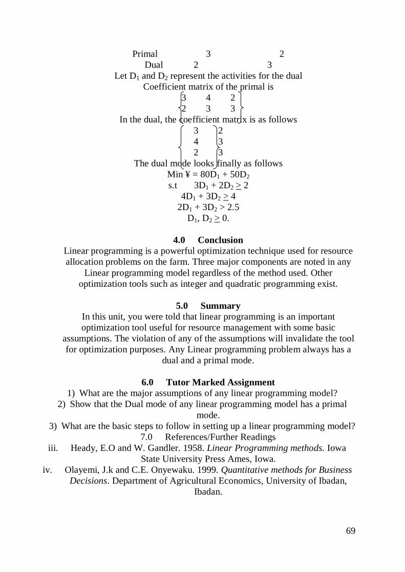
69

Primal 3 2 Dual 2 3

Let D1 and D2 represent the activities for the dual Coefficient matrix of the primal is

3 4 2 2 3 3

In the dual, the coefficient matrix is as follows 3 2 4 3 2 3

The dual mode looks finally as follows Min ¥ = 80D1 + 50D2 s.t 3D1 + 2D2 > 2

4D1 + 3D2 > 4 2D1 + 3D2 > 2.5

D1, D2 > 0.

4.0 Conclusion Linear programming is a powerful optimization technique used for resource allocation problems on the farm. Three major components are noted in any

Linear programming model regardless of the method used. Other optimization tools such as integer and quadratic programming exist.

5.0 Summary

In this unit, you were told that linear programming is an important optimization tool useful for resource management with some basic

assumptions. The violation of any of the assumptions will invalidate the tool for optimization purposes. Any Linear programming problem always has a

dual and a primal mode.

6.0 Tutor Marked Assignment 1) What are the major assumptions of any linear programming model?

2) Show that the Dual mode of any linear programming model has a primal mode.

3) What are the basic steps to follow in setting up a linear programming model? 7.0 References/Further Readings

iii. Heady, E.O and W. Gandler. 1958. Linear Programming methods. Iowa State University Press Ames, Iowa.

iv. Olayemi, J.k and C.E. Onyewaku. 1999. Quantitative methods for Business Decisions. Department of Agricultural Economics, University of Ibadan,

Ibadan.

AEC 403 COURSE TITLE: Agricultural Production Economics ...

Documents

Transcript of AEC 403 COURSE TITLE: Agricultural Production Economics ...