Advances in Nonlinear Waves and Symbolic Computation
76
Advances in Nonlinear Waves and Symbolic Computation Edited By Zhenya Yan Key Laboratory of Mathematics Mechanization Institute of Systems Science, Chinese Academy of Sciences, Beijing 100080, P. R. China Nova Science Publishers, Inc. New York
-
Upload
khangminh22 -
Category
Documents
-
view
4 -
download
0
Transcript of Advances in Nonlinear Waves and Symbolic Computation

Advances in Nonlinear Waves andSymbolic Computation
Edited By
Zhenya Yan
Key Laboratory of Mathematics Mechanization
Institute of Systems Science, Chinese Academy of Sciences,
Beijing 100080, P. R. China
Nova Science Publishers, Inc.
New York


Contents
1 Direct Methods and Symbolic Software for Conservation Laws of NonlinearEquations 11.1 Introduction . . . . . . . . . . . . . . . . . . . . . . . . . . . . . . . . . . 41.2 The Most Famous Example in Historical Perspective . . . . . . . . . . . . 71.3 The Method of Undetermined Coefficients . . . . . . . . . . . . . . . . . . 9
1.3.1 Dilation Invariance of Nonlinear PDEs . . . . . . . . . . . . . . . 91.3.2 The Method of Undetermined Coefficients Applied to a Scalar Non-
linear PDE . . . . . . . . . . . . . . . . . . . . . . . . . . . . . . 101.4 Tools from the Calculus of Variations and Differential Geometry . . . . . . 12
1.4.1 The Continuous Variational Derivative (Euler Operator) . . . . . . 131.4.2 The Continuous Homotopy Operator . . . . . . . . . . . . . . . . . 14
1.5 Conservation Laws of Nonlinear Systems of Polynomial PDEs . . . . . . . 151.5.1 Tools for Systems of Evolution Equations . . . . . . . . . . . . . . 161.5.2 The Drinfel’d-Sokolov-Wilson System: Dilation Invariance and Con-
servation Laws . . . . . . . . . . . . . . . . . . . . . . . . . . . . 161.5.3 Computation of a Conservation Law of the Drinfel’d-Sokolov Wil-
son System . . . . . . . . . . . . . . . . . . . . . . . . . . . . . . 171.5.4 The Boussinesq Equation: Dilation Invariance and Conservation
Laws . . . . . . . . . . . . . . . . . . . . . . . . . . . . . . . . . 191.5.5 Computation of a Conservation Law for the Boussinesq System . . 20
1.6 Conservation Laws of Systems of PDEs with Transcendental Nonlinearities 221.6.1 The sine-Gordon Equation: Dilation Invariance and Conservation
Laws . . . . . . . . . . . . . . . . . . . . . . . . . . . . . . . . . 221.6.2 Computation of a Conservation Law for the sine-Gordon System . . 23
1.7 Conservation Laws of Scalar Equations with Transcendental and MixedDerivative Terms . . . . . . . . . . . . . . . . . . . . . . . . . . . . . . . 251.7.1 The sine-Gordon Equation in Light-Cone Coordinates . . . . . . . 251.7.2 Examples of Equations with Transcendental Nonlinearities . . . . . 26
1.8 Nonlinear DDEs and Conservation Laws . . . . . . . . . . . . . . . . . . . 281.9 The Method of Undetermined Coefficients for DDEs . . . . . . . . . . . . 31
i

ii CONTENTS
1.9.1 A Classic Example: The Kac-van Moerbeke Lattice . . . . . . . . . 311.9.2 The Method of Undetermined Coefficients Applied to a Scalar Non-
linear DDE . . . . . . . . . . . . . . . . . . . . . . . . . . . . . . 321.10 Discrete Euler and Homotopy Operators . . . . . . . . . . . . . . . . . . . 341.11 Conservation Laws of Nonlinear Systems of DDEs . . . . . . . . . . . . . 36
1.11.1 The Toda Lattice . . . . . . . . . . . . . . . . . . . . . . . . . . . 371.11.2 Computation of a Conservation Law of the Toda Lattice . . . . . . 371.11.3 The Ablowitz-Ladik Lattice . . . . . . . . . . . . . . . . . . . . . 391.11.4 Computation of a Conservation Law of the Ablowitz-Ladik Lattice 401.11.5 A “Divide and Conquer” Strategy . . . . . . . . . . . . . . . . . . 41
1.12 A New Method to Compute Conservation Laws of Nonlinear DDEs . . . . 421.12.1 Leading Order Analysis . . . . . . . . . . . . . . . . . . . . . . . 431.12.2 A“Modified” Volterra Lattice . . . . . . . . . . . . . . . . . . . . 45
1.13 The Gardner Lattice . . . . . . . . . . . . . . . . . . . . . . . . . . . . . . 461.13.1 Derivation of the Gardner Lattice . . . . . . . . . . . . . . . . . . 471.13.2 Dilation Invariance of the Gardner Lattice . . . . . . . . . . . . . . 501.13.3 Conservation Laws of the Gardner Lattice . . . . . . . . . . . . . . 51
1.14 Additional Examples of Nonlinear DDEs . . . . . . . . . . . . . . . . . . 521.14.1 The Bogoyavlenskii Lattice . . . . . . . . . . . . . . . . . . . . . 521.14.2 The Belov-Chaltikian Lattice . . . . . . . . . . . . . . . . . . . . . 531.14.3 The Blaszak-Marciniak Lattices . . . . . . . . . . . . . . . . . . . 53
1.15 Software to Compute Conservation Laws for PDEs and DDEs . . . . . . . 541.15.1 Our Mathematica and Maple Software . . . . . . . . . . . . . . . . 551.15.2 Software Packages of Other Researchers . . . . . . . . . . . . . . . 55
1.16 Summary . . . . . . . . . . . . . . . . . . . . . . . . . . . . . . . . . . . 56

Preface
iii
iv CONTENTS

Chapter 1
Direct Methods and SymbolicSoftware for Conservation Laws ofNonlinear Equations
Willy Hereman1,a, Paul J. Adams1, Holly L. Eklund1,Mark S. Hickman2, and Barend M. Herbst3
1Department of Mathematical and Computer Sciences, Colorado School of Mines,Golden, CO 80401-1887, U.S.A.aE-mail: [email protected]
2Department of Mathematics and Statistics, University of Canterbury,Private Bag 4800, Christchurch 8140, New Zealand
3Department of Mathematical Sciences, Applied Mathematics Division,General Engineering Building, University of Stellenbosch
Private Bag X1, Matieland 7602, South Africa.
1

2 W. Hereman, P.J. Adams, H. L. Eklund, M.S. Hickman and B. M. Herbst
IN MEMORY OF MARTIN D. KRUSKAL (1925-2006)
Courtesy of Rutgers, The State University of New Jersey. Photographer, Nick Romanenko

Direct Methods and Symbolic Software for Conservation Laws 3
Abstract
We present direct methods, algorithms, and symbolic software for the computationof conservation laws of nonlinear partial differential equations (PDEs) and differential-difference equations (DDEs).
Our method for PDEs is based on calculus, linear algebra, and variational calculus.First, we compute the dilation symmetries of the given nonlinear system. Next, we builda candidate density as a linear combination with undetermined coefficients of terms thatare scaling invariant. The variational derivative (Euler operator) is used to derive a linearsystem for the undetermined coefficients. This system is then analyzed and solved. Finally,we compute the flux with the homotopy operator.
The method is applied to nonlinear PDEs in (1+1) dimensions with polynomial nonlin-earities which include the Korteweg-de Vries (KdV), Boussinesq, and Drinfel’d-Sokolov-Wilson equations. An adaptation of the method is applied to PDEs with transcendentalnonlinearities. Examples include the sine-Gordon, sinh-Gordon, and Liouville equations.For equations in laboratory coordinates, the coefficients of the candidate density are un-determined functions which must satisfy a mixed linear system of algebraic and ordinarydifferential equations.
For the computation of conservation laws of nonlinear DDEs we use a splitting of theidentity operator. This method is more efficient that an approach based on the discreteEuler and homotopy operators. We apply the method of undetermined coefficients to theKac-van Moerbeke, Toda, and Ablowitz-Ladik lattices. To overcome the shortcomings ofthe undetermined coefficient technique, we designed a new method that first calculates theleading order term and then the required terms of lower order. That method, which is nolonger restricted to polynomial conservation laws, is applied to discretizations of the KdVand modified KdV equations, and a combination thereof. Additional examples includelattices due to Bogoyavlenskii, Belov-Chaltikian, and Blaszak-Marciniak.
The undetermined coefficient methods for PDEs and DDEs have been implemented inMathematica. The code TransPDEDensityFlux.m computes densities and fluxesof systems of PDEs with or without transcendental nonlinearities. The code DDEDensityFlux.m does the same for polynomial nonlinear DDEs. Starting from the leading or-der terms, the new Maple library discrete computes densities and fluxes of nonlinearDDEs.
The software can be used to answer integrability questions and to gain insight in thephysical and mathematical properties of nonlinear models. When applied to nonlinear sys-tems with parameters, the software computes the conditions on the parameters for conser-vation laws to exist. The existence of a hierarchy of conservation laws is a predictor forcomplete integrability of the system and its solvability with the Inverse Scattering Trans-form.

4 W. Hereman, P.J. Adams, H. L. Eklund, M.S. Hickman and B. M. Herbst
1.1 Introduction
This chapter focuses on symbolic methods to compute polynomial conservation laws ofpartial differential equations (PDEs) in (1+1) dimensions and differential-difference equa-tions (DDEs), which are semi-discrete lattices. For the latter we treat systems where timeis continuous and the spatial variable has been discretized.
Nonlinear PDEs that admit conservation laws arise in many disciplines of the appliedsciences including physical chemistry, fluid mechanics, particle and quantum physics, plasmaphysics, elasticity, gas dynamics, electromagnetism, magneto-hydro-dynamics, nonlinearoptics, and the bio-sciences. Conservation laws are fundamental laws of physics that main-tain that a certain quantity will not change in time during physical processes. Familiarconservation laws include conservation of momentum, mass (matter), electric charge, orenergy. The continuity equation of electromagnetic theory is an example of a conservationlaw which relates charge to current. In fluid dynamics, the continuity equation expressesconservation of mass, and in quantum mechanics the conservation of probability of thedensity and flux functions also yields a continuity equation.
There are many reasons to compute conserved densities and fluxes of PDEs explicitly.Invariants often lead to new discoveries as was the case in soliton theory. One may want toverify if conserved quantities of physical importance (e.g. momentum, energy, Hamiltoni-ans, entropy, density, charge) are intact after constitutive relations have been added to closea system. For PDEs with arbitrary parameters one may wish to compute conditions on theparameters so that the model admits conserved quantities. Conserved densities also facili-tate the study of qualitative properties of PDEs [86, 97], such as recursion operators, bi- ortri-Hamiltonian structures, and the like. They often guide the choice of solution methodsor reveal the nature of special solutions. For example, an infinite sequence of conserveddensities is a predictor of the existence of solitons [7] and complete integrability [2] whichmeans that the PDE can be solved with the Inverse Scattering Transform (IST) method [2].
Conserved densities aid in the design of numerical solvers for PDEs [87, 88] and theirstability analysis (see references in [23]). Indeed, semi-discretizations that conserve dis-crete conserved quantities lead to stable numerical schemes that are free of nonlinear in-stabilities and blowup. While solving DDEs, which arise in nonlinear networks and assemi-discretizations of PDEs, one should check that their conserved quantities indeed re-main unchanged as time steps are taken.
Computer algebra systems (CAS) like Mathematica, Maple, and REDUCE, cangreatly assist the computation of conservation laws of nonlinear PDEs and DDEs. UsingCAS interactively, one can make a judicious guess (ansatz) and find a few simple densitiesand fluxes. Yet, that approach is fruitless for complicated systems with nontrivial con-servation laws with increasing complexity. Furthermore, completely integrable equationsPDEs [2,7,74,89] and DDEs [10,75] admit infinitely many independent conservation laws.Computing them is a challenging task. It involves tedious computations which are prone to

Direct Methods and Symbolic Software for Conservation Laws 5
error if done with pen and paper. Kruskal and collaborators demonstrated the complexitiesof calculating conservation laws in their seminal papers [67, 78, 79] on the Korteweg-deVries (KdV) equation from soliton theory [2,7,30]. We use this historical example to intro-duce the method of undetermined coefficients.
In the first part of this chapter we cover the symbolic computation of conservationlaws of completely integrable PDEs in (1 + 1) dimensions (with independent variables xand t). Our approach [8, 38, 51, 53] uses the concept of dilation (scaling) invariance andthe method of undetermined coefficients. Our method proceeds as follows. First, builda candidate density as a linear combination (with undetermined coefficients) of “buildingblocks” that are homogeneous under the scaling symmetry of the PDE. If no such symmetryexists, construct one by introducing parameters with scaling. Next, use the Euler operator(variational derivative) to derive a linear algebraic system for the undetermined coefficients.After the system is analyzed and solved, use the homotopy operator to compute the flux.When applied to systems with parameters, our codes can determine the conditions on theparameters so that a sequence of conserved densities exists.
The method is applied to nonlinear PDEs in (1 + 1) dimensions with polynomial termswhich include the KdV, Boussinesq, and Drinfel’d-Sokolov-Wilson equations. An adapta-tion of the method is applied to PDEs with transcendental nonlinearities. Examples includethe sine-Gordon, sinh-Gordon, and Liouville equations. For equations written in laboratorycoordinates, the coefficients of the candidate density are undetermined functions whichmust satisfy a mixed linear system of algebraic and ordinary differential equations (ODEs).
Capitalizing on the analogy between PDEs and DDEs, the second part of this chapterdeals with the symbolic computation of conservation laws of nonlinear DDEs [33, 39, 42,51,54,57]. Again, we use scaling symmetries and the method of undetermined coefficients.One could use discrete versions of the Euler operator (to verify exactness) and the homo-topy operator (to invert the forward difference). Although these operators might be valuablein theory, they are highly inefficient as tools for the symbolic computation of conservationlaws of DDEs. We advocate the use of a “splitting and shifting” technique, which allows usto compute densities and fluxes simultaneously at minimal cost. The undetermined coeffi-cient method for DDEs is illustrated with the Kac-van Moerbeke, Toda, and Ablowitz-Ladiklattices.
There is a fundamental difference between the continuous and discrete cases in theway densities are constructed. The total derivative has a weight whereas the shift operatordoes not. Consequently, a density of a PDE is bounded in order with respect to the spacevariable. Unfortunately, there is no a priori bound on the number of shifts in the density,unless a leading order analysis is carried out. To overcome this difficulty and other short-comings of the undetermined coefficient method, we present a new method to computeconserved densities of DDEs. That method no longer uses dilation invariance and is nolonger restricted to polynomial conservation laws. Instead of building a candidate densitywith undetermined coefficients, one first computes the leading order term in the density

6 W. Hereman, P.J. Adams, H. L. Eklund, M.S. Hickman and B. M. Herbst
and, secondly, generates the required terms of lower order. The method is fast and effi-cient since unnecessary terms are never computed. The new method is illustrated using amodified Volterra lattice as an example. The new method performs exceedingly well whenapplied to lattices due to Bogoyavlenskii, Belov-Chaltikian, and Blaszak-Marciniak. Thenew method is also applied to completely integrable discretizations of the KdV and mod-ified KdV (mKdV) equations, and a combination thereof, known as the Gardner equation.Starting from a discretized eigenvalue problem, we first derive the Gardner lattice and thencompute conservation laws.
There are several methods (see [51]) to compute conservation laws of nonlinear PDEsand DDEs. Some methods use a generating function [2,7], which requires the knowledge ofkey pieces of the IST. Another common approach uses the link between conservation lawsand symmetries as stated in Noether’s theorem [14, 15, 66, 81]. However, the computationof generalized (variational) symmetries, though algorithmic, is as daunting a task as thedirect computation of conservation laws. Most of the more algorithmic methods [12,13,20,25, 63, 101], require the solution of a determining system of ODEs or PDEs. Despite theirpower, only a few of these methods have been implemented in CAS. We devote a sectionto symbolic software for the computation of conservation laws. Additional reviews can befound in [38, 51, 101].
Over the past decade, in collaboration with students and researchers, we have de-signed and implemented direct algorithms for the computation of conservation laws ofnonlinear PDEs and DDEs. We purposely avoid Noether’s theorem, pre-knowledge ofsymmetries, and a Lagrangian formulation. Neither do we use differential forms or ad-vanced differential-geometric tools. Instead, we concentrate on the undetermined coeffi-cient method for PDEs and DDEs, which uses tools from calculus, linear algebra, and thevariational calculus. Therefore, the method is easy to implement in Mathematica andeasy to use by scientists and engineers. The code TransPDEDensityFlux.m computesdensities and fluxes of systems of PDEs with or without transcendental nonlinearities. Thecode DDEDensityFlux.m does the same for polynomial nonlinear DDEs. Starting fromthe leading order terms, the new Maple library discrete computes densities and fluxesof nonlinear DDEs very efficiently. The software can thus be used to answer integrabil-ity questions and to gain insight in the physical and mathematical properties of nonlinearmodels.
Our software is in the public domain. The Mathematica packages and notebooksare available at [48] and Hickman’s code in Maple is available at [56]. We are currentlyworking on a comprehensive package to compute conservation laws of PDEs in multiplespace dimensions [45, 51, 83].
Part I: Partial Differential Equations in (1 + 1) DimensionsIn this first part we cover PDEs in (1 + 1) dimensions, that is, PDEs in one space variableand time. Starting from a historical example, we introduce the concept of dilation invariance

Direct Methods and Symbolic Software for Conservation Laws 7
and use the method of undetermined coefficients to compute conservation laws of evolutionequations. Later on, we adapt the method of undetermined coefficients to cover PDEs withtranscendental terms.
1.2 The Most Famous Example in Historical Perspective
The story of conservation laws for nonlinear PDEs begins with the discovery of an infinitenumber of conservation laws of the ubiquitous Korteweg-de Vries equation which models avariety of nonlinear wave phenomena, including shallow water waves [46] and ion-acousticwaves in plasmas [2, 7, 30]. The KdV equation can be recast in dimensionless variables as
ut + αuux + u3x = 0, (1.1)
where the subscripts denote partial derivatives, i.e. ut = ∂u∂t , ux = ∂u
∂x , and u3x = ∂3u∂x3 .
The parameter α can be scaled to any real number. Commonly used values are α = ±1 orα = ±6.
Equation (1.1) is an example of a scalar (1 + 1)−dimensional evolution equation,
ut = F (x, t, u, ux, u2x, · · · , unx), (1.2)
of order n in the independent space variable x and of first order in time t. Obviously, thedependent variable is u(x, t). If parameters are present in (1.2), they will be denoted bylower-case Greek letters. A conservation law of (1.2) is of the form
Dt ρ+ Dx J = 0, (1.3)
which is satisfied for all solutions u(x, t) of the PDE. In physics, ρ is called the conserveddensity (or charge); J is the associated flux (or current). In general, both are differentialfunctions (functionals), i.e. functions of x, t, u, and partial derivatives of u with respect tox. In (1.3), Dx denotes the total derivative with respect to x, that is,
DxJ =∂J
∂x+
N∑k=0
∂J
∂ukxu(k+1)x, (1.4)
where N is the order of J, and Dt is the total derivative with respect to t, defined by
Dt ρ =∂ρ
∂t+ ρ′[ut] =
∂ρ
∂t+
M∑k=0
∂ρ
∂ukxDkxut, (1.5)
where ρ′[ut] is the Frechet derivative of ρ in the direction of ut and M is the order of ρ.The densities ρ(1) = u and ρ(2) = u2 of (1.1) were long known. In 1965, Whitham
[98] had found a third density, ρ(3) = u3 − 3αu
2x, which, in the context of water waves,

8 W. Hereman, P.J. Adams, H. L. Eklund, M.S. Hickman and B. M. Herbst
corresponds to Boussinesq’s moment of instability [76]. One can readily verify that
Dt(u) + Dx(12αu
2 + u2x) = 0, (1.6)
Dt(u2) + Dx(23αu
3 − u2x + 2uu2x) = 0, (1.7)
Dt(u3 − 3αu
2x) + Dx(3
4αu4 − 6uu2
x + 3u2u2x + 3αu
22x − 6
αuxu3x) = 0. (1.8)
Indeed, (1.6) is the KdV equation written as a conservation law; (1.7) is obtained aftermultiplying (1.1) by 2u; (1.8) requires more work. Hence, the first three density-flux pairsof (1.1) are
ρ(1) = u, J (1) = 12αu
2 + u2x, (1.9)
ρ(2) = u2, J (2) = 23αu
3 − u2x + 2uu2x, (1.10)
ρ(3) = u3 − 3αu
2x, J (3) = 3
4αu4 − 6uu2
x + 3u2u2x + 3αu
22x − 6
αuxu3x. (1.11)
Integrals of motion readily follow from the densities. Indeed, assuming that J vanishes atinfinity (for example due to sufficiently fast decay of u and its x derivatives), upon integra-tion of (1.3) with respect to x one obtains that
P =∫ ∞−∞
ρ dx (1.12)
is constant in time. Such constants of motion also arise when u is periodic, in whichcase one integrates over the finite period. Depending on the physical setting, the first fewconstants of motion (i.e. integrals (1.12)) express conservation of mass, momentum, andenergy.
Martin Kruskal and postdoctoral fellow Norman Zabusky discovered the fourth and fifthdensities for the KdV equation [111]. However, they failed in finding a sixth conservationlaw due to an algebraic mistake in their computations. Kruskal asked Robert Miura, alsopostdoctoral fellow at the Princeton Plasma Physics Laboratory at New Jersey, to searchfor further conservation laws of the KdV equation. Miura [78] computed the seventh con-servation law. After correcting the mistake mentioned before, he also found the sixth andeventually three additional conservation laws. Rumor [80] has it that in the summer of 1966Miura went up into the Canadian Rockies and returned from the mountains with the first 10conservation laws of the KdV equation engraved in his notebook. This biblical metaphorprobably does not do justice to Miura’s intense and tedious work with pen and paper.
With ten conservation laws in hand, it was conjectured that the KdV equation had aninfinite sequence of conservation laws, later proven to be true [67, 79]. Aficionados of ex-plicit formulas can find the first ten densities (and seven of the associated fluxes) in [79] andthe eleventh density (with 45 terms) in [67], where a recursion formula is given to generateall further conserved densities. As an aside, in 1966 the first five conserved densities werecomputed on an IBM 7094 computer with FORMAC, an early CAS. The sixth density couldno longer be computed because the available storage space was exceeded. In contrast, using

Direct Methods and Symbolic Software for Conservation Laws 9
a method of undetermined coefficients, the first eleven densities were computed in 1969 ona AEC CDC-6600 computer in a record time of 2.2 seconds. Due to limitations in handlinglarge integers, the computer could not correctly produce any further densities.
Undoubtedly, the discovery of conservation laws played a pivotal role in the compre-hensive study of the properties and solutions of nonlinear completely integrable PDEs (likethe KdV equation) and the development of the IST (see e.g. [80] for the history). CliffordGardner, John Greene, Martin Kruskal, and Robert Miura received the 2006 Leroy P. SteelePrize [115], awarded by the American Mathematical Society, for their seminal contributionto research on the KdV equation. In turn, Martin Kruskal has received numerous honors andawards [114] for his fundamental contributions to the understanding of integrable systemsand soliton theory. This chapter is dedicated to Martin Kruskal (1925-2006).
1.3 The Method of Undetermined Coefficients
We now sketch the method of undetermined coefficients to compute conservation laws [38,96], which draws on ideas and observations in before mentioned work by Kruskal andcollaborators.
1.3.1 Dilation Invariance of Nonlinear PDEs
Crucial to the computation of conservation laws is that (1.3) must hold on the PDE. Thisis achieved by substituting ut (and utx, utxx, etc.) from (1.1) in the evaluation of (1.6)-(1.8) and in all subsequent conservation laws of degree larger than 3. The eliminationof all t−derivatives of u in favor of x derivatives has two important consequences: (i)any symmetry of the PDE, in particular, the dilation symmetry, will be adopted by theconservation law, (ii) once Dt is computed and evaluated on the PDE, t becomes a parameterin the computation of the flux.
We will first investigate the dilation (scaling) symmetry of evolution equations. TheKdV equation is dilation invariant under the scaling symmetry
(t, x, u)→ (λ−3t, λ−1x, λ2u), (1.13)
where λ is an arbitrary parameter. Indeed, after a change of variables with t = λ−3t, x =λ−1x, u = λ2u, and cancellation of a common factor λ5, the KdV for u(x, t) arises. Thedilation symmetry of (1.1) can be expressed as
u ∼ ∂2
∂x2,
∂
∂t∼ ∂3
∂x3, (1.14)
which means that u corresponds to two x−derivatives and the time derivative corresponds tothree x−derivatives. If we define the weight, W, of a variable (or operator) as the exponentof λ in (1.13), then W (x) = −1 or W ( ∂
∂x) = 1;W (t) = −3 or W ( ∂∂t) = 3, and W (u) =2.

10 W. Hereman, P.J. Adams, H. L. Eklund, M.S. Hickman and B. M. Herbst
All weights of dependent variables and the weights of ∂/∂x, ∂/∂t, are assumed to benon-negative and rational. The rank of a monomial is defined as the total weight of themonomial. Such monomials may involve the independent and dependent variables and theoperators ∂
∂x ,Dx,∂∂t , and Dt. Ranks must be positive integers or positive rational numbers.
An expression (or equation) is uniform in rank if its monomial terms have equal rank.For example, (1.1) is uniform in rank since each of the three terms has rank 5.
Conversely, if one does not know the dilation symmetry of (1.1), then it can be readilycomputed by requiring that (1.1) is uniform in rank. Indeed, setting W (∂/∂x) = 1 andequating the ranks of the three terms in (1.1) gives
W (u) +W (∂
∂t) = 2W (u) + 1 = W (u) + 3, (1.15)
which yields W (u) = 2,W (∂/∂t) = 3, and, in turn, confirms (1.13). So, requiring uni-formity in rank of a PDE allows one to compute the weights of the variables (and thus thescaling symmetry) with linear algebra.
Dilation symmetries, which are special Lie-point symmetries, are common to manynonlinear PDEs. Needless to say, not every PDE is dilation invariant, but non-uniform PDEscan be made uniform by extending the set of dependent variables with auxiliary parameterswith appropriate weights. Upon completion of the computations one can set these parame-ters to one. In what follows, we setW (∂/∂x) = W (Dx) = 1 andW (∂/∂t) = W (Dt).Ap-plied to (1.6), rank ρ(1) = 2, rank J (1) = 4. Hence, rank (Dt ρ
(1)) = rank (Dx J(1)) = 5.
Therefore, (1.6) is uniform of rank 5. In (1.7), rank ρ(2) = 4 and rank J (2) = 6, conse-quently, (1.7) is uniform of rank 7.
In (1.11), each term in ρ(3) has rank 6 and each term in J (3) has rank 8. Consequently,rank (Dt ρ
(3)) = rank (Dx J(3)) = 9, which makes (1.8) is uniform of rank 9. All densities
of (1.1) are uniform in rank and so are the associated fluxes and the conservation laws.Equation (1.1) also has density-flux pairs that depend explicitly on t and x; for example,
ρ = tu2 +2αxu, J = t
(23αu3 − u2
x + 2uu2x
)− x
(u2 − 2
αu2x
)+
2αux. (1.16)
Since W (x) = −1 and W (t) = −3, one has rank ρ = 1, and rank J = 3. The methodsand algorithms discussed in subsequent sections have been adapted to compute densitiesand fluxes explicitly dependent on x and t. Instead of addressing this issue in this chapter,we refer the reader to [38, 53].
1.3.2 The Method of Undetermined Coefficients Applied to a Scalar Nonlin-ear PDE
We outline how densities and fluxes can be constructed for a scalar evolution equation (1.2).To keep matters transparent, we illustrate the steps for the KdV equation resulting in ρ(3)
of rank R = 6 with associated flux J (3) of rank 8, both listed in (1.11). The tools neededfor the computations will be presented in the next section.

Direct Methods and Symbolic Software for Conservation Laws 11
• Select the rank R of ρ. Make a list, R, of all monomials in u and its x-derivatives sothat each monomial has rank R. This can be done as follows. Starting from the set V ofdependent variables (including parameters with weight, when applicable), make a setM ofall non-constant monomials of rank R or less (but without x−derivatives). Next, for eachterm in M, introduce the right number of x−derivatives to adjust the rank of that term.Distribute the x−derivatives, strip off the numerical coefficients, and gather the resultingterms in a set R. For the KdV equation and R = 6, V = {u} andM = {u3, u2, u}. Sinceu3, u2, and u have ranks 6, 4 and 2, respectively, one computes
∂0u3
∂x0= u3,
∂2u2
∂x2= 2u2
x + 2uu2x,∂4u
∂x4= u4x. (1.17)
Ignoring numerical coefficients in the right hand sides of the equations in (1.17), one getsR = {u3, u2
x, uu2x, u4x}.• Remove fromR all monomials that are total x−derivatives. Also remove all “equivalent”monomials, i.e. the monomials that differ from another by a total x−derivative, keeping themonomial of lowest order. Call the resulting set S. In our example, u4x must be removed(because u4x = Dxu3x) and uu2x must be removed since uu2x and u2
x are equivalent.Indeed, uu2x = Dx(uux)− u2
x. Thus, S = {u3, u2x}.
• Linearly combine the monomials in S with constant undetermined coefficients ci to obtainthe candidate ρ. Continuing with the example,
ρ = c1 u3 + c2 u
2x, (1.18)
which is of first order in x.
• Using (1.5), compute Dt ρ. Applied to (1.18) where M = 1, one gets
Dt ρ = (3c1u2I + 2c2uxDx)[ut]. (1.19)
As usual, D0x = I is the identity operator.
• Evaluate−Dt ρ on the PDE (1.2) by replacing ut by F. The result is a differential functionE in which t is a parameter. For the KdV equation (1.1), F = −(αuux + u3x). Afterreversing the sign, the evaluated form of (1.19) is
E = (3c1u2I + 2c2uxDx)(αuux + u3x)
= 3c1αu3ux + 2c2αu3x + 2c2αuuxu2x + 3c1u2u3x + 2c2uxu4x. (1.20)
• To obtain a conservation law, E must be a total derivative. Starting with highest orders,repeatedly integrate E by parts. Doing so, allows one to write E as the sum of a totalx−derivative, Dx J, and a non-integrable part (i.e. the obstructing terms). J is the (candi-

12 W. Hereman, P.J. Adams, H. L. Eklund, M.S. Hickman and B. M. Herbst
date) flux with rank J = R+W (Dt)− 1. Integration by parts of (1.20) gives
E = Dx(34c1αu
4 + 3c1u2u2x + c2αuu2x + 2c2uxu3x)− 6c1uuxu2x
−2c2u2xu3x + c2αu3x
= Dx(34c1αu
4 − 3c1uu2x + c2αuu
2x + 3c1u2u2x + 2c2uxu3x − c2u2
2x)
+(3c1 + c2α)u3x. (1.21)
The candidate flux therefore is
J =34c1αu
4 − 3c1uu2x + c2αuu
2x + 3c1u2u2x + 2c2uxu3x − c2u2
2x. (1.22)
• Equate the coefficients of the obstructing terms to zero. Solve the linear system for theundetermined coefficients ci. In the example (3c1 + c2α)u3
x is the only obstructing termwhich vanishes for c2 = − 3
αc1, where c1 is arbitrary.
• Substitute the coefficients ci into ρ and J to obtain the final forms of the density andassociated flux (with a common arbitrary factor which can be set to 1). Setting c1 = 1 andsubstituting c2 = − 3
α into (1.18) and (1.22) yields ρ(3) and J (3) as given in (1.11).
Constructing “minimal” densities, i.e. densities which are free of equivalent terms and totalderivatives terms, becomes challenging if the rank R is high. Furthermore, integration byparts is cumbersome and prone to mistakes if done by hand. Moreover, it would be advan-tageous if the integration by parts could be postponed until the undetermined coefficients cihave been computed and substituted in E. Ideally, the computations of the density and theflux should be decoupled. There is a need for computational tools to address these issues,in particular, if one wants to compute conservation laws of systems of evolution equations.
1.4 Tools from the Calculus of Variations and Differential Ge-ometry
A scalar differential function E of order M is called exact (integrable) if and only if thereexists a scalar differential function J of order M − 1 such that E = Dx J. Obviously,J = D−1
x E =∫E dx is then the primitive (or integral) of E. Two questions arise: (i) How
can one test whether or not E is exact? (ii) If E is exact, how can one compute J withoutusing standard integration by parts? To answer the first question we will use the variationalderivative (Euler operator) from the calculus of variations. To perform integration by partswe will use the homotopy operator from differential geometry.

Direct Methods and Symbolic Software for Conservation Laws 13
1.4.1 The Continuous Variational Derivative (Euler Operator)
The continuous variational derivative, also called the Euler operator of order zero , L(0)u(x),
for variable u(x) is defined [81] by
L(0)u(x)E =
M∑k=0
(−Dx)k∂E
∂ukx
=∂E
∂u− Dx
∂E
∂ux+ D2
x
∂E
∂u2x− D3
x
∂E
∂u3x+ · · ·+ (−1)MDM
x
∂E
∂uMx, (1.23)
where E is a differential function in u(x) of order M.
A necessary and sufficient condition for a differential function E to be exact is thatL(0)u(x)E ≡ 0. A proof of this statement is given in e.g. [67]. If L(0)
u(x)E 6= 0, then E is not atotal x−derivative due to obstructing terms.
Application 1. Returning to (1.20), we now use the variational derivative to determine c1and c2 so that E of order M = 4 will be exact. Using nothing but differentiations, wereadily compute
L(0)u(x)E =
∂E
∂u− Dx
∂E
∂ux+ D2
x
∂E
∂u2x− D3
x
∂E
∂u3x+ D4
x
∂E
∂u4x
= 9c1αu2ux + 2c2αuxu2x + 6c1uu3x − Dx(3c1αu3 + 6c2αu2x
+2c2αuu2x + 2c2u4x) + D2x(2c2αuux)− D3
x(3c1u2) + D4x(2c2ux)
= (9c1αu2ux + 2c2αuxu2x + 6c1uu3x)− (9c1αu2ux + 14c2αuxu2x
+2c2αuu3x + 2c2u5x) + (6c2αuxu2x + 2c2αuu3x)
−(18c1uxu2x + 6c1uu3x) + (2c2u5x)
= −6(3c1 + c2α)uxu2x. (1.24)
Note that the terms in u2ux, uu3x, and u5x dropped out. Hence, requiring that L(0)u(x)E ≡ 0
leads to 3c1+c2α = 0. Substituting c1 =1, c2 = − 3α , into (1.18) yields ρ(3) in (1.11).
Application 2. It is paramount that the candidate density is free of total x−derivativesand equivalent terms. If such terms were present, they could be moved into the flux J,and their coefficients ci would be arbitrary. ρ(1) and ρ(2), are equivalent if and only ifρ(1) + kρ(2) = Dx J, for some J and non-zero scalar k. We write ρ(1) ≡ ρ(2). Clearly ρ isequivalent to any non-zero multiple of itself and ρ ≡ 0 if and only if ρ is exact.
Instead of working with different densities, we investigate the equivalence of terms ti inthe same density. For example, returning to the setR = {u3, u2
x, uu2x, u4x}, terms t2 = u2x
and t3 = uu2x are equivalent because t3 + t2 = uu2x + u2x = Dx(uux).
The variational derivative can be used to detect equivalent and exact terms. Indeed, notethat v1 = L(0)
u(x)(uu2x) = 2u2x and v2 = L(0)u(x)u
2x = −2u2x are linearly dependent. Also,
for t4 = u4x = Dxu3x one gets v3 = L(0)u(x)u4x = 0. To weed out the terms ti inR that are

14 W. Hereman, P.J. Adams, H. L. Eklund, M.S. Hickman and B. M. Herbst
equivalent or total derivatives, it suffices to check the linear independence of their imagesvi under the Euler operator.
One can optimize this procedure by starting from a setR where some of the equivalentand total derivatives terms have been removed a priori. Indeed, in view of (1.17), one canignore the highest-order terms (typically the last terms) in each of the right hand sides.Therefore, R = {u3, u2
x} and, for this example, no further reduction would be necessary.Various algorithms are possible to construct minimal densities. Details are given in [38,51].
1.4.2 The Continuous Homotopy Operator
We now discuss the homotopy operator [12, 13, 52, 81] which will allow one to reduce thecomputation of J = D−1
x E =∫E dx to a single integral with respect to an auxiliary
variable denoted by λ (not to be confused with λ in Section 1.3.1). Hence, the homotopyoperator circumvents integration by parts and reduces the inversion of Dx to a problem ofsingle-variable calculus.
The homotopy operator [81, p. 372] for variable u(x), acting on an exact expression Eof order M, is given by
Hu(x)E =∫ 1
0(IuE) [λu]
dλ
λ, (1.25)
where the integrand IuE is given by
IuE =M∑k=1
(k−1∑i=0
uix(−Dx)k−(i+1)
)∂E
∂ukx. (1.26)
In (1.25), (IuE)[λu] means that in IuE one replaces u → λu, ux → λux, etc. Thisis a special case of the homotopy, λ(u(1) − u(0)) + u(0), between two points, u(0) =(u0, u0
x, u02x, · · · , u0
Mx) and u(1) = (u1, u1x, u
12x, · · · , u1
Mx), in the jet space. For our pur-poses we set u(0) = (0, 0, · · · , 0) and u(1) = (u, ux, u2x, · · · , uMx). Formula (1.26) isequivalent to the one in [52], which in turn is equivalent to the formula in terms of higherEuler operators [45, 51].
Given an exact differential function E of order M one has J = D−1x E =
∫E dx =
Hu(x)E. A proof of this statement can be found in [52].
Application. After substituting c1 = 1 and c2 = − 3α into (1.20) we obtain the exact
expression
E = 3αu3ux − 6u3x − 6uuxu2x + 3u2u3x −
6αuxu4x, (1.27)

Direct Methods and Symbolic Software for Conservation Laws 15
of order M = 4. First, using (1.26), we compute
IuE =4∑
k=1
(k−1∑i=0
uix(−Dx)k−(i+1)
)∂E
∂ukx
= (uI)(∂E
∂ux) + (uxI− uDx)(
∂E
∂u2x) + (u2xI− uxDx + uD2
x)(∂E
∂u3x)
+(u3xI− u2xDx + uxD2x − uD3
x)(∂E
∂u4x). (1.28)
After substitution of (1.27), one gets
IuE = (uI)(3αu3 + 18u2x − 6uu2x −
6αu4x) + (uxI− uDx)(−6uux)
+(u2xI− uxDx + uD2x)(3u2) + (u3xI− u2xDx + uxD
2x − uD3
x)(− 6αux)
= 3αu4 − 18uu2x + 9u2u2x +
6αu2
2x −12αuxu3x, (1.29)
which has the correct terms of J (3) but incorrect coefficients. Finally, using (1.25),
J =Hu(x)E =∫ 1
0(IuE)[λu]
dλ
λ
=∫ 1
0
(3αλ3u4 − 18λ2uu2
x + 9λ2u2u2x +6αλu2
2x −12αλuxu3x
)dλ
=34αu4 − 6uu2
x + 3u2u2x +3αu2
2x −6αuxu3x, (1.30)
which matches J (3) in (1.11).
The crux of the homotopy operator method [12, 13, 26, 81] is that the integration byparts of a differential expression like (1.27), which involves an arbitrary function u(x) andits x−derivatives, can be reduced to a standard integration of a polynomial in λ.
1.5 Conservation Laws of Nonlinear Systems of Polynomial PDEs
Thus far we have dealt with the computation of density-flux pairs of scalar evolution equa-tions, with the KdV equation as the leading example. In this section we show how themethod and tools can be generalized to cover systems of evolution equations. We will usethe Drinfel’d-Sokolov-Wilson system and the Boussinesq equation to illustrate the steps.

16 W. Hereman, P.J. Adams, H. L. Eklund, M.S. Hickman and B. M. Herbst
1.5.1 Tools for Systems of Evolution Equations
For differential functions (like densities and fluxes) of two dependent variables (u, v) andtheir x−derivatives, the total derivatives are
Dtρ =∂ρ
∂t+
M1∑k=0
∂ρ
∂ukxDkx ut +
M2∑k=0
∂ρ
∂vkxDkx vt, (1.31)
DxJ =∂J
∂x+
N1∑k=0
∂J
∂ukxu(k+1)x +
N2∑k=0
∂J
∂vkxv(k+1)x, (1.32)
where M1 and M2 are the (highest) orders of u and v in ρ, and N1 and N2 are the (highest)orders of u and v in J.
To accommodate two dependent variables, we need Euler operators L(0)u(x) and L(0)
v(x)
for each dependent variable separately. For brevity, we will use vector notation, that is,L(0)
u(x)E = (L(0)u(x)E,L
(0)v(x)E). Likewise, the homotopy operator in (1.25) must be replaced
by
Hu(x)E =∫ 1
0(IuE + IvE)[λu]
dλ
λ, (1.33)
where
IuE =M1∑k=1
(k−1∑i=0
uix(−Dx)k−(i+1)
)∂E
∂ukx, (1.34)
and
IvE =M2∑k=1
(k−1∑i=0
vix(−Dx)k−(i+1)
)∂E
∂vkx, (1.35)
where M1,M2 are the orders of E in u, v, respectively. In (1.33), u → λu, ux →λux, · · · , v → λv, vx → λvx, etc.
1.5.2 The Drinfel’d-Sokolov-Wilson System: Dilation Invariance and Con-servation Laws
We consider a parameterized family of the Drinfel’d-Sokolov-Wilson (DSW) equations
ut + 3vvx = 0, vt + 2uvx + αuxv + 2v3x = 0, (1.36)
where α is a nonzero parameter. The system with α = 1 was first proposed by Drin-fel’d and Sokolov [31, 32] and Wilson [99]. It can be obtained [59] as a reduction of theKadomtsev-Petviashvili equation (i.e. a two-dimensional version of the KdV equation) andis a completely integrable system. In [109], Yao and Li computed conservation laws of(1.36), where they had introduced four arbitrary coefficients. Using scales on x, t, u and v,all but one coefficients in (1.36) can be scaled to any real number. Therefore, to cover the

Direct Methods and Symbolic Software for Conservation Laws 17
entire family of DSW equations it suffices to leave one coefficient arbitrary, e.g. α in frontof uxv.
To compute the dilation symmetry of (1.36), we assign weights, W (u) and W (v), toboth dependent variables and express that each equation separately must be uniform in rank(i.e. the ranks of the equations in (1.36) may differ from each other).
For the DSW equations (1.36), one has
W (u) +W (∂/∂t) = 2W (v) + 1,
W (v) +W (∂/∂t) = W (u) +W (v) + 1 = W (v) + 3, (1.37)
which yields W (u) = W (v) = 2, W (∂/∂t) = 3. The DSW system (1.36) is thus invariantunder the scaling symmetry
(x, t, u, v)→ (λ−1x, λ−3t, λ2u, λ2v), (1.38)
where λ is an arbitrary scaling parameter.The first three density-flux pairs for the DSW equations (1.36) are
ρ(1) = u, J (1) =32v2, (1.39)
ρ(2) = v, J (2) = 2(uv + v2x), if α = 2, (1.40)
ρ(3) = (α− 1)u2 +32v2, J (3) = 3(αuv2 − v2
x + 2vv2x), (1.41)
Both ρ(1) and ρ(2) have rank 2; their fluxes have rank 4. The pair (ρ(1), J (1)) exists for anyα, whereas (ρ(2), J (2)) only exists if α = 2. Density ρ(3) of rank 4 and flux J (3) of rank 6are valid for any α. At rank R = 6,
ρ(4) = (α+ 1)(α− 2)u3 − 92
(α+ 1)uv2 − 32
(α− 2)u2x −
272v2x. (1.42)
The corresponding flux (not shown) has 7 terms. At rank R = 8,
ρ(5) = u4 − 92u2v2 − 27
8v4 − 9
2uu2
x +34u2
2x +452vuxvx + 27uv2
x −814v22x, (1.43)
provided α = 1. The corresponding flux (not shown) has 15 terms. There exists a density-flux pair for all even ranks R ≤ 10 provided α = 1, for which (1.36) is completely inte-grable.
1.5.3 Computation of a Conservation Law of the Drinfel’d-Sokolov WilsonSystem
To illustrate how the presence of a parameter, like α, affects the computation of densities,we compute ρ(1) and ρ(2) of rank R = 2 given in (1.39) and (1.40).

18 W. Hereman, P.J. Adams, H. L. Eklund, M.S. Hickman and B. M. Herbst
Step 1: Construct the form of the density
The set of dependent variables is V = {u, v}.Both elements are of rank 2 so, no x−derivativesare needed. Thus, M = R = S = {u, v}. Linearly combining the elements in S givesρ = c1u+ c2v.
Step 2: Compute the undetermined coefficients ciEvaluating E = −Dtρ = −(c1ut + c2vt) on (1.36), yields
E = 3c1vvx + c2(2uvx + αuxv + 2v3x), (1.44)
which will be exact if L(0)u(x)E = (L(0)
u(x)E,L(0)v(x)E) ≡ (0, 0). Since E is of order M1 = 1
in u and order M2 = 3 in v,
L(0)u(x)E =
∂E
∂u− Dx
∂E
∂ux= 2c2vx − Dx(c2αv) = (2− α)c2vx, (1.45)
and
L(0)v(x)E =
∂E
∂v− Dx
∂E
∂vx+ D2
x
∂E
∂v2x− D3
x
∂E
∂v3x= 3c1vx + c2αux − Dx(3c1v + 2c2u)− D3
x(2c2)
= (α− 2)c2ux. (1.46)
Both (1.45) and (1.46) will vanish identically if and only if (α − 2)c2 = 0. This equation(with unknowns c1 and c2) is parameterized by α 6= 0. The solution algorithm [38] consid-ers all branches of the solution and possible compatibility conditions. Setting c1 = 1, leadsto either (i) c2 = 0 if α 6= 2, or (ii) c2 arbitrary if α = 2. Setting c2 = 1 leads to the com-patibility condition, α = 2, and c1 arbitrary. Substituting the solutions into ρ = c1u+ c2v
gives ρ = u which is valid for any α; and ρ = u + c2v or ρ = c1u + v provided α = 2.In other words, ρ(1) = u is the only density of rank 2 for arbitrary values of α. For α = 2there exist two independent densities, ρ(1) = u and ρ(2) = v.
Step 3: Compute the associated flux J
As an example, we compute the flux in (1.40) associated with ρ(2) = v and α = 2. In thiscase, c1 = 0, c2 = 1, for which (1.44) simplifies into
E = 2(uvx + uxv + v3x), (1.47)
which is of order M1 = 1 in u and order M2 = 3 in v. Using (1.34) and (1.35), we obtain
IuE = (uI)∂E
∂ux= (uI)(2v) = 2uv, (1.48)
and
IvE = (vI)(∂E
∂vx) + (vxI− vDx)(
∂E
∂v2x) + (v2xI− vxDx + vD2
x)(∂E
∂v3x)
= (vI)(2u) + (v2xI− vxDx + vD2x)(2)
= 2uv + 2v2x. (1.49)

Direct Methods and Symbolic Software for Conservation Laws 19
Hence, using (1.33),
J = Hu(x)E =∫ 1
0(IuE+ IvE)[λu]
dλ
λ=∫ 1
0(4λuv+ 2v2x) dλ = 2(uv+ v2x), (1.50)
which is J (2) in (1.40). The integration of (1.47) could easily be done by hand. The ho-motopy operator method pays off if the expression to be integrated has a large number ofterms.
1.5.4 The Boussinesq Equation: Dilation Invariance and Conservation Laws
The wave equation,u2t − u2x + 3u2
x + 3uu2x + αu4x = 0, (1.51)
for u(x, t) with real parameter α, was proposed by Boussinesq to describe surface waves inshallow water [2]. For what follows, we rewrite (1.51) as a system of evolution equations,
ut + vx = 0, vt + ux − 3uux − αu3x = 0, (1.52)
where v(x, t) is an auxiliary dependent variable.The Boussinesq system (1.52) is not uniform in rank because the terms ux and αu3x
lead to an inconsistent system of weight equations. To circumvent the problem we introducean auxiliary parameter β with (unknown) weight, and replace (1.52) by
ut + vx = 0, vt + βux − 3uux − αu3x = 0. (1.53)
Requiring uniformity in rank, we obtain (after some algebra)
W (u) = 2, W (v) = 3, W (β) = 2, W (∂
∂t) = 2. (1.54)
Therefore, (1.53) is invariant under the scaling symmetry
(x, t, u, v, β)→ (λ−1x, λ−2t, λ2u, λ3v, λ2β). (1.55)
As the above example shows, a PDE that is not dilation invariant can be made so by ex-tending the set of dependent variables with one or more auxiliary parameters with weights.Upon completion of the computations one can set each of these parameters equal to 1.
The Boussinesq equation (1.51) has infinitely many conservation laws and is completelyintegrable [2, 7]. The first four density-flux pairs [8] for (1.53) are
ρ(1) = u, J (1) = v, (1.56)
ρ(2) = v, J (2) = βu− 32u
2 − αu2x, (1.57)
ρ(3) = uv, J (3) = 12βu
2 − u3 + 12v
2 + 12αu
2x − αuu2x, (1.58)
ρ(4) = βu2 − u3 + v2 + αu2x,
J (4) = 2βuv − 3u2v + 2αuxvx − 2αu2xv. (1.59)

20 W. Hereman, P.J. Adams, H. L. Eklund, M.S. Hickman and B. M. Herbst
These densities are of ranks 2, 3, 5 and 6, respectively. The corresponding fluxes are of onerank higher. After setting β = 1 we obtain the conserved quantities of (1.52) even thoughinitially this system was not uniform in rank.
1.5.5 Computation of a Conservation Law for the Boussinesq System
We show the computation of ρ(4) and J (4) of ranks 6 and 7, respectively. The presence ofthe auxiliary parameter β with weight complicates matters. At a fixed rank R, conserveddensities corresponding to lower ranks might appear in the result. These lower-rank densi-ties are easy to recognize for they are multiplied with arbitrary coefficients ci.Consequently,when parameters with weight are introduced, the densities corresponding to distinct ranksare no longer linearly independent. As the example below will show, densities must be splitinto independent pieces.
Step 1: Construct the form of the density
Augment the set of dependent variables with the parameter β (with non-zero weight).Hence, V = {u, v, β}. Construct M = {β2u, βu2, βu, βv, u3, u2, u, v2, v, uv}, whichcontains all non-constant monomials of (chosen) rank 6 or less (without derivatives). Next,for each term inM, introduce the right number of x-derivatives so that each term has rank6. For example,
∂2βu
∂x2=βu2x,
∂2u2
∂x2=2u2
x + 2uu2x,∂4u
∂x4=u4x,
∂(uv)∂x
= vux + uvx, etc.. (1.60)
Gather the terms in the right hand sides of the equations in (1.60) to get
R = {β2u, βu2, u3, v2, vux, u2x, βvx, uvx, βu2x, uu2x, v3x, u4x}. (1.61)
Using (1.23) and a similar formula for v, for every term ti inRwe compute vi = L(0)u(x)ti =
(L(0)u(x)ti,L
(0)v(x)ti). If vi = (0, 0) then ti is discarded and so is vi. If vi 6= (0, 0) we verify
whether or not vi is linearly independent of the non-zero vectors vj , j = 1, 2, · · · , i − 1.If independent, the term ti is kept, otherwise, ti is discarded and so is vi.
Upon application of L(0)u(x), the first six terms in R lead to linearly independent vectors
v1 through v6. Therefore, t1 through t6 are kept (and so are the corresponding vectors).For t7 = βvx we compute v7 =L(0)
u(x)(βvx) = (0, 0). So, t7 is discarded and so is v7. For
t8 = uvx we get v8 =L(0)u(x)(uvx)=(vx,−ux) = −v5. So, t8 is discarded and so is v8.
Proceeding in a similar fashion, t9, t10, t11 and t12 are discarded. Thus, R is replacedby
S = {β2u, βu2, u3, v2, vux, u2x}, (1.62)
which is free of divergences and divergence-equivalent terms. Ignoring the highest-orderterms (typically the last terms) in each of the right hand sides of the equations in (1.60)

Direct Methods and Symbolic Software for Conservation Laws 21
optimizes the procedure. Indeed, R would have had six instead of twelve terms. Coinci-dentally, in this example no further eliminations would be needed to obtain S.Next, linearlycombine the terms in S to get
ρ = c1β2u+ c2βu
2 + c3u3 + c4v
2 + c5vux + c6u2x. (1.63)
Step 2: Compute the undetermined coefficients ciCompute Dtρ. Here, ρ is of order M1 =1 in u and order M2 =0 in v. Hence, application of(1.31) gives
Dtρ =∂ρ
∂uIut +
∂ρ
∂uxDxut +
∂ρ
∂vIvt
= (c1β2 + 2c2βu+ 3c3u2)ut + (c5v + 2c6ux)utx + (2c4v + c5ux)vt. (1.64)
Use (1.53) to eliminate ut, utx, and vt. Then, E=−Dt ρ evaluates to
E = (c1β2 + 2c2βu+ 3c3u2)vx + (c5v + 2c6ux)v2x+(2c4v + c5ux)(βux − 3uux − αu3x), (1.65)
which must be exact. Thus, require that L(0)u(x)E = (L(0)
u(x)E,L(0)v(x)E) ≡ (0, 0). Group like
terms. Set their coefficients equal to zero to obtain the parameterized system
β(c2 − c4) = 0, c3 + c4 = 0, c5 = 0, αc5 = 0, βc5 = 0, αc4 − c6 = 0, (1.66)
where α 6= 0 and β 6= 0. Investigate the eliminant of the system. Set c1 = 1 and obtain thesolution
c1 = 1, c2 = c4, c3 = −c4, c5 = 0, c6 = αc4, (1.67)
which holds without condition on α and β. Substitute (1.67) into (1.63) to get
ρ = β2u+ c4(βu2 − u3 + v2 + αu2x). (1.68)
The density must be split into independent pieces. Indeed, since c4 is arbitrary, set c4 = 0or c4 = 1, thus splitting (1.68) into two independent densities
ρ = β2u ≡ u, ρ = βu2 − u3 + v2 + αu2x, (1.69)
which are ρ(1) and ρ(4) in (1.56)-(1.59).
Step 3: Compute the flux J
Compute the flux corresponding to ρ in (1.69). Substitute (1.67) into (1.65). Take the termsin c4 and set c4 = 1. Thus,
E = 2βuvx + 2βvux − 3u2vx − 6uvux + 2αuxv2x − 2αvu3x, (1.70)

22 W. Hereman, P.J. Adams, H. L. Eklund, M.S. Hickman and B. M. Herbst
which is of order M1 = 3 in u and order M2 = 2 in v. Using (1.34) and (1.35), one readilyobtains
IuE = 2βuv − 6u2v + 2αuxvx − 2αu2xv, (1.71)
andIvE = 2βuv − 3u2v + 2αuxvx − 2αu2xv. (1.72)
Hence, using (1.33),
J = Hu(x)E =∫ 1
0(IuE + IvE)[λu]
dλ
λ
=∫ 1
0
(4βλuv − 9λ2u2v + 4αλuxvx − 4αλu2xv
)dλ
= 2βuv − 3u2v + 2αuxvx − 2αu2xv, (1.73)
which is J (4) in (1.59). One can set β = 1 at the end of the computations.
1.6 Conservation Laws of Systems of PDEs with TranscendentalNonlinearities
We now turn to the symbolic computation of conservation laws of certain classes of PDEswith transcendental nonlinearities. We only consider PDEs where the transcendental func-tions act on one dependent variable u (and not on x−derivatives of u). In contrast to theexamples in the previous sections, the candidate density will no longer have constant unde-termined coefficients but functional coefficients which depend on the variable u. Further-more, we consider only PDEs which have one type of nonlinearity. For example, sine, orcosine, or exponential terms are fine but not a mixture of these functions.
1.6.1 The sine-Gordon Equation: Dilation Invariance and Conservation Laws
The sine-Gordon (sG) equation appears in the literature [17, 69] in two different ways:
• In light-cone coordinates the sG equation, uxt = sinu, has a mixed derivative term, whichcomplicates matters. We return to this type of equation in Section 1.7.1.
• The sG equation in laboratory coordinates , u2t − u2x = sinu, can be recast as
ut + v = 0, vt + u2x + sinu = 0, (1.74)
where v(x, t) is an auxiliary variable. System (1.74) is amenable to our approach, subjectto modifications to accommodate the transcendental nonlinearity.
The sG equation describes the propagation of crystal dislocations, superconductivity ina Josephson junction, and ultra-short optical pulse propagation in a resonant medium [69].In mathematics, the sG equation is long known in the differential geometry of surfaces ofconstant negative Gaussian curvature [30, 80].
Direct Methods and Symbolic Software for Conservation Laws 23
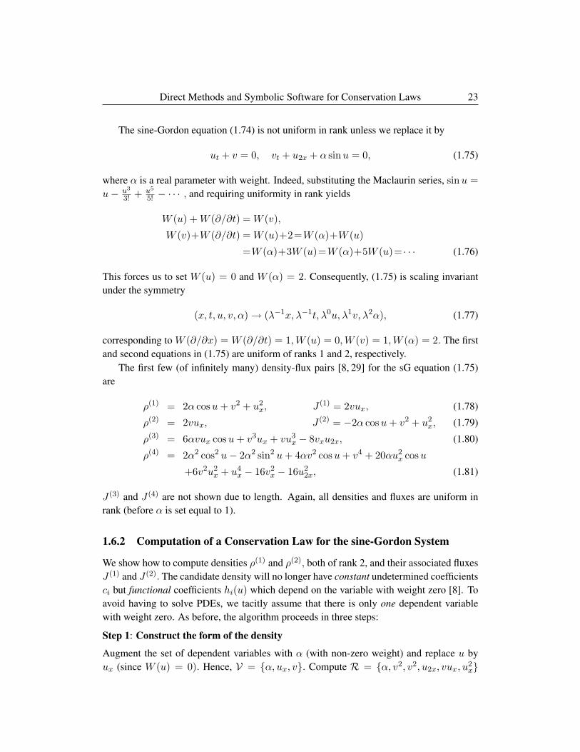
The sine-Gordon equation (1.74) is not uniform in rank unless we replace it by
ut + v = 0, vt + u2x + α sinu = 0, (1.75)
where α is a real parameter with weight. Indeed, substituting the Maclaurin series, sinu =u− u3
3! + u5
5! − · · · , and requiring uniformity in rank yields
W (u) +W (∂/∂t) = W (v),
W (v)+W (∂/∂t) = W (u)+2=W (α)+W (u)
=W (α)+3W (u)=W (α)+5W (u)= · · · (1.76)
This forces us to set W (u) = 0 and W (α) = 2. Consequently, (1.75) is scaling invariantunder the symmetry
(x, t, u, v, α)→ (λ−1x, λ−1t, λ0u, λ1v, λ2α), (1.77)
corresponding to W (∂/∂x) = W (∂/∂t) = 1,W (u) = 0,W (v) = 1,W (α) = 2. The firstand second equations in (1.75) are uniform of ranks 1 and 2, respectively.
The first few (of infinitely many) density-flux pairs [8, 29] for the sG equation (1.75)are
ρ(1) = 2α cosu+ v2 + u2x, J (1) = 2vux, (1.78)
ρ(2) = 2vux, J (2) = −2α cosu+ v2 + u2x, (1.79)
ρ(3) = 6αvux cosu+ v3ux + vu3x − 8vxu2x, (1.80)
ρ(4) = 2α2 cos2 u− 2α2 sin2 u+ 4αv2 cosu+ v4 + 20αu2x cosu
+6v2u2x + u4
x − 16v2x − 16u2
2x, (1.81)
J (3) and J (4) are not shown due to length. Again, all densities and fluxes are uniform inrank (before α is set equal to 1).
1.6.2 Computation of a Conservation Law for the sine-Gordon System
We show how to compute densities ρ(1) and ρ(2), both of rank 2, and their associated fluxesJ (1) and J (2). The candidate density will no longer have constant undetermined coefficientsci but functional coefficients hi(u) which depend on the variable with weight zero [8]. Toavoid having to solve PDEs, we tacitly assume that there is only one dependent variablewith weight zero. As before, the algorithm proceeds in three steps:
Step 1: Construct the form of the density
Augment the set of dependent variables with α (with non-zero weight) and replace u byux (since W (u) = 0). Hence, V = {α, ux, v}. Compute R = {α, v2, v2, u2x, vux, u
2x}

24 W. Hereman, P.J. Adams, H. L. Eklund, M.S. Hickman and B. M. Herbst
and remove divergences and equivalent terms to get S = {α, v2, u2x, vux}. The candidate
densityρ = αh1(u) + h2(u)v2 + h3(u)u2
x + h4(u)vux, (1.82)
with undetermined functional coefficients hi(u).
Step 2: Compute the functions hi(u)
Compute
Dtρ =∂ρ
∂uIut +
∂ρ
∂uxDxut +
∂ρ
∂vIvt
= (αh′1 + v2h′2 + u2xh′3 + vuxh
′4)ut + (2uxh3 + vh4)utx
+(2vh2 + uxh4)vt, (1.83)
where h′i denotes dhidu . After replacing ut and vt from (1.75), E = −Dtρ becomes
E = (αh′1 + v2h′2 + u2xh′3 + vuxh
′4)v + (2uxh3 + vh4)vx
+(2vh2 + uxh4)(α sinu+ u2x). (1.84)
E must be exact. Therefore, require that L(0)u(x)E ≡ 0 and L(0)
v(x)E ≡ 0. Set the coefficientsof like terms equal to zero to get a mixed linear system of algebraic equations and ODEs:
h2(u)− h3(u)=0, h′2(u)=0, h′3(u)=0, h′4(u)=0, h′′2(u)=0,
h′′4(u) = 0, 2h′2(u)− h′3(u) = 0, 2h′′2(u)− h′′3(u) = 0, (1.85)
h′1(u) + 2h2(u) sinu = 0, h′′1(u) + 2h′2(u) sinu+ 2h2(u) cosu = 0.
Solve the system [8] and substitute the solution
h1(u) = 2c1 cosu+ c3, h2(u) = h3(u) = c1, h4(u) = c2, (1.86)
(with arbitrary constants ci) into (1.82) to obtain
ρ = c1(2α cosu+ v2 + u2x) + c2vux + c3α. (1.87)
Step 3: Compute the flux J
Compute the flux corresponding to ρ in (1.87). Substitute (1.86) into (1.84), to get
E = c1(2uxvx + 2vu2x) + c2(αux sinu+ vvx + uxu2x). (1.88)
Since E = DxJ, one must integrate to obtain J. Using (1.26) and (1.35) one gets IuE =2c1vux + c2(αu sinu+ u2
x) and IvE=2c1vux + c2v2. Using (1.33),
J = Hu(x)E =∫ 1
0(IuE + IvE)[λu]
dλ
λ
=∫ 1
0
(4c1λvux + c2(αu sin(λu) + λv2 + λu2
x))dλ
= c1(2vux) + c2(−α cosu+ 1
2v2 + 1
2u2x
). (1.89)

Direct Methods and Symbolic Software for Conservation Laws 25
Finally, split density (1.87) and flux (1.89) into independent pieces (for c1 and c2) to get
ρ(1) = 2α cosu+ v2 + u2x, J (1) = 2vux, (1.90)
ρ(2) = vux, J (2) = −α cosu+ 12v
2 + 12u
2x. (1.91)
For E in (1.88), J in (1.89) can easily be computed by hand [8]. However, the computationof fluxes corresponding to densities of ranks ≥ 2 is cumbersome and requires integrationwith the homotopy operator.
1.7 Conservation Laws of Scalar Equations with Transcendentaland Mixed Derivative Terms
Our method to compute densities and fluxes of scalar equations with transcendental termsand a mixed derivative term (i.e. uxt) is an adaptation of the technique shown in Section 1.5.We only consider single PDEs with one type of transcendental nonlinearity. Since we areno longer dealing with evolution equations, densities and fluxes could dependent on ut, u2t,
etc. We do not cover such cases; instead, we refer the reader to [101].
1.7.1 The sine-Gordon Equation in Light-Cone Coordinates
In light-cone coordinates (or characteristic coordinates) the sG equation,
uxt = sinu, (1.92)
has a mixed derivative as well as a transcendental term. A change of variables, Φ = ux,Ψ =−1 + cosu, allows one to replace (1.92) by
Φxt − Φ− ΦΨ = 0, 2Ψ + Ψ2 + Φ2t = 0, (1.93)
without transcendental terms. Unfortunately, neither (1.92) nor (1.93) can be written as asystem of evolution equations. As shown in Section 1.6.1, to deal with the transcendentalnonlinearity, which imposes W (u) = 0, one has to replace (1.92) by
uxt = α sinu, (1.94)
where α is an auxiliary parameter with weight. Indeed, (1.94) is dilation invariant under thescaling symmetry
(x, t, u, α)→ (λ−1x, λ−1t, λ0u, λ2α), (1.95)

26 W. Hereman, P.J. Adams, H. L. Eklund, M.S. Hickman and B. M. Herbst
corresponding toW (∂/∂x) = W (∂/∂t) = 1,W (u) = 0, andW (α) = 2. The density-fluxpairs [8, 29] of ranks 2, 4, 6, and 8 (which are independent of ut, u2t, etc.), are
ρ(1) = u2x, J (1) = 2α cosu, (1.96)
ρ(2) = u4x − 4u2
2x J (2) = 4αu2x cosu, (1.97)
ρ(3) = u6x − 20u2
xu22x + 8u2
3x,
J (3) = 2α(3u4x cosu+ 8u2
xu2x sinu− 4u22x cosu), (1.98)
ρ(4) = 5u8x − 280u4
xu22x − 112u4
2x + 224u2xu
23x − 64u2
4x, (1.99)
J (4) = 8α(5u6
x cosu+ 40u4xu2x sinu+ 20u2
xu22x cosu+ 16u3
2x sinu
−16u3xu3x cosu− 48uxu2xu3x sinu+ 8u2
3x cosu). (1.100)
There are infinitely many density-flux pairs (all of even rank). Since uxt = (ux)t, one canview (1.94) as an evolution equation in a new variable, U = ux, and construct densitiesas linear combinations with constant coefficients of monomials in U and its x−derivatives.As before, each monomial has a (pre-selected) rank. To accommodate the transcendentalterm(s) one might be incorrectly tempted to linearly combine such monomials with func-tional coefficients hi(u) instead of constant coefficients ci. For example, however, for rankR = 2, one should take ρ = c1u
2x instead of ρ = h1(u)u2
x, because the latter would lead toDtρ = h′1utu
2x + 2h1uxu2x and ut cannot be replaced from (1.94).
1.7.2 Examples of Equations with Transcendental Nonlinearities
In this section we consider additional PDEs of the form uxt = f(u), where f(u) hastranscendental terms. Using the Painleve integrability test, researchers [12] have concludedthat the only PDEs of that type that are completely integrable are equivalent to one ofthe standard forms of the nonlinear Klein-Gordon equation [2, 12]. These standard forms(in light-cone coordinates) include the sine-Gordon equation, uxt = sinu, discussed inSection 1.6.1, the sinh-Gordon equation uxt = sinhu, the Liouville equation uxt = eu,and the double Liouville equations, uxt = eu ± e−2u. The latter is also referred to in theliterature as the Tzetzeica and Mikhailov equations. For each of these equations one cancompute conservation laws with the method discussed in Section 1.7.1. Alternatively, ifthese equations were transformed into laboratory coordinates, one would apply the methodof Section 1.6.2. The multiple sine-Gordon equations, e.g. uxt = sinu+sin 2u, have only afinite number of conservation laws and are not completely integrable, as supported by otherevidence [2].
The sinh-Gordon equation, uxt = sinhu, arises as a special case of the Toda latticediscussed in Section 1.11.1. It also describes the dynamics of strings in constant curva-ture space-times [70]. In thermodynamics, the sinh-Gordon equation can be used to cal-culate partition and correlation functions, and thus support Langevin simulations [64]. InTable 1.1, we show a few density-flux pairs for the sinh-Gordon equation in light-cone co-ordinates, uxt = α sinhu. As with the sG equation (1.92), W (∂/∂x) = W (∂/∂t) = 1,

Direct Methods and Symbolic Software for Conservation Laws 27
W (u) = 0, and W (α) = 2. The ranks in the first column of Table 1.1 correspond tothe ranks of the densities, which are polynomial in U = ux and its x−derivatives. Thesinh-Gordon equation has infinitely many conservation laws and is known to be completelyintegrable [2].
Table 1.1: Conservation Laws of the sinh-Gordon equation, uxt = α sinhu
Rank Density (ρ) Flux (J)2 u2
x −2α coshu4 u4
x + 4u22x −4αu2
x coshu6 u6
x + 20u2xu
22x + 8u2
3x −2α[(3u4x + 4u2
2x) coshu+ 8u2xu2x sinhu]
8 5u8x + 280u4
xu22x + 64u2
4x −8α[(5u6
x − 20u2xu
22x + 16u3
xu3x + 8u23x) coshu
+224u2xu
23x − 112u4
2x +(40u4xu2x − 16u3
2x + 48uxu2xu3x) sinhu].
The Liouville equation, uxt = eu, plays an important role in modern field theory [68],e.g. in the theory of strings, where the quantum Liouville field appears as a conformalanomaly [65]. The first few (of infinitely many) density-flux pairs for the Liouville equationin light-cone coordinates, uxt = αeu, are given in Table 1.2. As before, W (∂/∂x) =W (∂/∂t) = 1, W (u) = 0, and W (α) = 2. The ranks in the table refer to the ranks of thedensities. Dodd and Bullough [29] have shown that the Liouville equation has no densitiesof ranks 3, 5, and 7. As shown in Table 1.2, there are two densities of rank 6, and threedensities of rank 8. Our results agree with those in [29], where one can also find the uniquedensity of rank 9 and the four independent densities of rank 10.
The double Liouville equations,
uxt = eu ± e−2u, (1.101)
arise in the field of “laser-induced vibrational predesorption of molecules physisorbed oninsulating substrates.” More precisely, (1.101) is used to investigate the dynamics of en-ergy flow of excited admolecules on insulating substrates [82]. Double Liouville equationsare also relevant in studies of global properties of scalar-vacuum configurations in generalrelativity and similarly systems in alternative theories of gravity [22].
In Table 1.3, we show some density-flux pairs of uxt = α(eu − e−2u). There are nodensity-flux pairs for ranks 4 and 10. We computed a density-flux pair for rank 12 (notshown due to length). The results for (1.101) with the plus sign are similar.
Part II: Nonlinear Differential-Difference EquationsIn the second part of this chapter we discuss two distinct methods to construct conservationlaws of nonlinear DDEs. The first method follows closely the technique for PDEs discussedin Part I. It is quite effective for certain classes of DDEs, including the Kac-van Moerbeke

28 W. Hereman, P.J. Adams, H. L. Eklund, M.S. Hickman and B. M. Herbst
Table 1.2: Conservation Laws of the Liouville equation, uxt = αeu
R Density (ρ) Flux (J)
2 u2x −2αeu
4 u4x + 4u2
2x −4αu2xeu
6 c1(u6x − 20u3
2x − 12u23x) −α
[6c1(u4
x − 4u2xu2x − 2u2
2x)
+c2(u2xu
22x + u3
2x + u23x) +c2u2x(2u2
x + u2x)]
eu
8 c1(u8x − 56u2
xu32x − 168u2
xu23x −α
[8c1(u6
x − 6u4xu2x + 3u2
xu22x − 20u3
2x
−672u2xu23x − 144u2
4x) −36u3xu3x − 108uxu2xu3x − 18u2
3x)
+c2(u4xu
22x + u2
xu32x + 5u2
xu23x +c2(2u4
xu2x − u2xu
22x + 4u3
2x + 8u3xu3x
+18u2xu23x + 4u2
4x) + c3(u42x +24uxu2xu3x + 4u2
3x)
+3u2xu
23x + 15u2xu
23x + 3u2
4x) +c3(4u32x + 6u3
xu3x + 18uxu2xu3x + 3u23x)]
eu
and Toda lattices, but far less effective for more complicated lattices, such as the Bogoy-avlenskii and the Gardner lattices. The latter examples are treated with a new method basedon a leading order analysis proposed by Hickman [55].
1.8 Nonlinear DDEs and Conservation Laws
We consider autonomous nonlinear systems of DDEs of the form
un = F(un−l, ...,un−1,un,un+1, ...,un+m), (1.102)
where un and F are vector-valued functions with N components. We only consider DDEswith one discrete variable, denoted by integer n. In many applications, n comes from adiscretization of a space variable. The dot stands for differentiation with respect to thecontinuous variable which frequently is time, t. We assume that F is polynomial with con-stant coefficients, although this restriction can be waived for the method presented in Sec-tion 1.12. No restrictions are imposed on the degree of nonlinearity of F. If parameters arepresent in (1.102), they will be denoted by lower-case Greek letters.
F depends on un and a finite number of forward and backward shifts of un.We identifyl with the furthest negative shift of any variable in the system, and m with the furthestpositive shift of any variable in the system. No restrictions are imposed on the integers land m, which measure the degree of non-locality in (1.102).
By analogy with Dx, we define the shift operator D by Dun = un+1. The operator D isoften called the up-shift operator or forward- or right-shift operator. Its inverse, D−1, is the

Direct Methods and Symbolic Software for Conservation Laws 29
Table 1.3: Conservation Laws of the double Liouville equation, uxt = α(eu − e−2u)
Rank Density (ρ) Flux (J)
2 u2x −α(2eu + e−2u)
4 —— ——
6 u6x + 15u2
xu22x − 5u3
2x + 3u23x −3α
[(2u4
x + 2u2xu2x + u2
2x)eu
+(u4x − 8u2
xu2x + 2u22x)e−2u
]8 u8
x + 42u4xu
22x − 14u2
xu32x − 7u4
2x −α[(8u6
x + 36u4xu2x − 18u2
xu22x − 20u3
2x
+21u2xu
23x − 21u2xu
23x + 3u2
4x +6u3xu3x + 18uxu2xu3x + 3u2
3x)eu
+(4u6x − 72u4
xu2x − 18u2xu
22x − 4u3
2x
+48u3xu3x − 72uxu2xu3x + 6u2
3x)e−2u]
10 —— ——
down-shift operator or backward- or left-shift operator, D−1un = un−1. The action of theshift operators is extended to functions by acting on their arguments. For example,
DF(un−l, ...,un−1,un,un+1, ...,un+m)
= F(Dun−l, ...,Dun−1,Dun,Dun+1, ...,Dun+m)
= F(un−l+1, ...,un,un+1,un+2, ...,un+m+1). (1.103)
Following [57], we generate (1.102) from
u0 = F(u−l,u−l+1, ...,u−1,u0,u1, ...,um−1,um), (1.104)
where un = Dnu0 = DnF. To further simplify the notation, we denote the zero-shifteddependent variable, u0, by u. Shifts of u are generated by repeated application of D. Forinstance, uk = Dku. The identity operator is denoted by I, where D0u = Iu = u.
A conservation law of (1.104),
Dt ρ+ ∆ J = 0, (1.105)
links a conserved density ρ to an associated flux J, where both are scalar functions de-pending on u and its shifts. In (1.105), which holds on solutions of (1.104), Dt is the totalderivative with respect to time and ∆ = D− I is the forward difference operator.
For readability (in particular, in the examples), the components of u will be denoted byu, v, w, etc. In what follows we consider only autonomous functions, i.e. F, ρ, and J do notexplicitly depend on t.

30 W. Hereman, P.J. Adams, H. L. Eklund, M.S. Hickman and B. M. Herbst
The time derivatives are defined in a similar way as in the continuous case, see (1.5) and(1.31). We show the discrete analog of (1.31). For a density ρ(up, up+1, · · · , uq, vr, vr+1, · · · ,vs), involving two dependent variables (u, v) and their shifts, the time derivative is com-puted as
Dtρ =q∑
k=p
∂ρ
∂ukuk +
s∑k=r
∂ρ
∂vkvk
=
q∑k=p
∂ρ
∂ukDk
u+
(s∑
k=r
∂ρ
∂vkDk
)v, (1.106)
since D and d/dt commute. Obviously, the difference operator extends to functions. Forexample, ∆J = D J − J for a flux, J.
A density is trivial if there exists a function ψ so that ρ = ∆ψ. Similar to the continuouscase, we say that two densities, ρ(1) and ρ(2), are equivalent if and only if ρ(1) + kρ(2) =∆ψ, for some ψ and some non-zero scalar k.
It is paramount that the density is free of equivalent terms for if such terms were present,they could be moved into the flux J. Instead of working with different densities, we will usethe equivalence of monomial terms ti in the same density (of a fixed rank). Compositions ofD or D−1 define an equivalence relation (≡) on monomial terms. Simply stated, all shiftedterms are equivalent, e.g. u−1v1 ≡ uv2 ≡ u2v4 ≡ u−3v−1 since
u−1v1 = uv2 −∆ (u−1v1) = u2v4 −∆ (u1v3 + uv2 + u−1v1)
= u−3v−1 + ∆ (u−2v + u−3v−1). (1.107)
This equivalence relation holds for any function of the dependent variables, but for theconstruction of conserved densities we will apply it only to monomials.
In the algorithm used in Sections 1.9.2, 1.11.2, and 1.11.4, we will use the followingequivalence criterion: two monomial terms, t1 and t2, are equivalent, t1 ≡ t2, if and onlyif t1 = Dr t2 for some integer r. Obviously, if t1 ≡ t2, then t1 = t2 + ∆J for somepolynomial J, which depends on u and its shifts. For example, u−2u ≡ u−1u1 becauseu−2u = D−1u−1u1. Hence, u−2u = u−1u1 + [−u−1u1 + u−2u] = u−1u1 + ∆J, withJ = −u−2u.
For efficiency we need a criterion to choose a unique representative from each equiva-lence class. There are a number of ways to do this. We define the canonical representativeas that member that has (i) no negative shifts and (ii) a non-trivial dependence on the local(that is, zero-shifted) variable. For example, uu2 is the canonical representative of the class{· · · , u−2u, u−1u1, uu2, u1u3, · · · }. In the case of e.g. two variables (u and v), u2v is thecanonical representative of the class {· · · , u−1v−3, uv−2, u1v−1, u2v, u3v1, · · · }.
Alternatively, one could choose a variable ordering and then choose the member thatdepends on the zero-shifted variable of lowest lexicographical order. The code in [48] uses

Direct Methods and Symbolic Software for Conservation Laws 31
lexicographical ordering of the variables, i.e. u ≺ v ≺ w, etc. Thus, uv−2 (instead of u2v)is chosen as the canonical representative of {· · · , u−1v−3, uv−2, u1v−1, u2v, u3v1, · · · }.
It is easy to show [55] that if ρ is a density then Dkρ is also a density. Hence, using anappropriate “up-shift” all negative shifts in a density can been removed. Thus, without lossof generality, we may assume that a density that depends on q shifts has canonical formρ(u,u1, · · · ,uq).
1.9 The Method of Undetermined Coefficients for DDEs
In this section we show how polynomial conservation laws can be computed for a scalarDDE,
u = F (u−l, u−l+1, · · · , u, · · · , um−1, um). (1.108)
The Kac-van Moerbeke example is used to illustrate the steps.
1.9.1 A Classic Example: The Kac-van Moerbeke Lattice
The Kac-van Moerbeke (KvM) lattice [60, 62], also known as the Volterra lattice,
un = un(un+1 − un−1), (1.109)
arises in the study of Langmuir oscillations in plasmas, population dynamics, etc. Eq.(1.109) appears in the literature in various forms, including Rn = 1
2(exp(−Rn−1) −exp(−Rn+1)), and wn = wn(w2
n+1 − w2n−1), which relate to (1.109) by simple trans-
formations [92]. We continue with (1.109) and, adhering to the simplified notation, write itas
u = u(u1 − u−1), (1.110)
or, with the conventions adopted above, u = u(Du− D−1u).Lattice (1.110) is invariant under the scaling symmetry (t, u) → (λ−1t, λu). Hence, u
corresponds to one derivative with respect to t, i.e. u ∼ ddt . In analogy to the continuous
case, we define the weight W of a variable as the exponent of λ that multiplies the variable[39, 40]. We assume that shifts of a variable have the same weights, that is, W (u−1) =W (u) = W (u1). Weights of dependent variables are nonnegative and rational. The rankof a monomial equals the total weight of the monomial. An expression (or equation) isuniform in rank if all its monomial terms have equal rank.
Applied to (1.110), W (d/dt) = W (Dt) = 1 and W (u) = 1. Conversely, the scalingsymmetry can be computed with linear algebra as follows. Setting W (d/dt) = 1 andrequiring that (1.110) is uniform in rank yields W (u) + 1 = 2W (u). Thus, W (u) = 1,which agrees with the scaling symmetry.
Many integrable nonlinear DDEs are scaling (dilation) invariant. If not, they can bemade so by extending the set of dependent variables with parameters with weights. Exam-ples of such cases are given in Sections 1.11.3 and 1.13.2.

32 W. Hereman, P.J. Adams, H. L. Eklund, M.S. Hickman and B. M. Herbst
The KvM lattice has infinitely many polynomial density-flux pairs. We give the con-served densities of rank R ≤ 4 with associated fluxes (J (4) is omitted due to length):
ρ(1) = u, J (1) =−uu−1, (1.111)
ρ(2) = 12u
2 + uu1, J (2) =−(u−1u2 − u−1uu1), (1.112)
ρ(3) = 13u
3 + uu1(u+ u1 + u2),
J (3) = −(u−1u3 + 2u−1u
2u1 + u−1uu21 + u−1uu1u2), (1.113)
ρ(4) = 14u
4 + u3u1 + 32u
2u21 + uu2
1(u1 + u2)
+uu1u2(u+ u1 + u2 + u3). (1.114)
In addition to infinitely many polynomial conserved densities, (1.110) has a non-polynomialdensity, ρ(0) = lnu with flux J (0) = −(u + u−1). We discuss the computation of non-polynomial densities in Section 1.12.
1.9.2 The Method of Undetermined Coefficients Applied to a Scalar Nonlin-ear DDE
We outline how densities and fluxes can be constructed for a scalar DDE (1.108). Using(1.110) as an example, we compute ρ(3) of rank R = 3 and associated flux J (3) of rankR = 4, both listed in (1.113).
• Select the rank R of ρ. Start from the set V of dependent variables (including parame-ters with weight, when applicable), and form a set M of all non-constant monomials ofrank R or less (without shifts). For each monomial in M introduce the right number oft−derivatives to adjust the rank of that term. Using the DDE, evaluate the t−derivatives,strip off the numerical coefficients, and gather the resulting terms in a set R. For the KvMlattice (1.110), V = {u} andM = {u3, u2, u}. Since u3, u2, and u have ranks 3, 2, and 1,respectively, one computes
d0u3
dt0= u3,
du2
dt= 2uu = 2u2(u1 − u−1) = 2u2u1 − 2u−1u
2, (1.115)
and
d2u
dt2=
dudt
=d (u(u1 − u−1))
dt= u(u1 − u−1) + u(u1 − u−1)
= u(u1 − u−1)2 + u(u1(u2 − u)− u−1(u− u−2))
= uu21 − 2u−1uu1 + u2
−1u+ uu1u2 − u2u1 − u−1u2 + u−2u−1u, (1.116)
where (1.110) (and its shifts) has been used to remove the time derivatives. Build R usingthe terms from the right hand sides of the equations in (1.115) and ignoring numericalcoefficients,
R={u3, u2u1, u−1u2, uu2
1, u−1uu1, u2−1u, uu1u2, u−2u−1u}. (1.117)

Direct Methods and Symbolic Software for Conservation Laws 33
• Identify the elements in R that belong to the same equivalence classes, replace themby their canonical representatives, and remove all duplicates. Call the resulting set S,which has the building blocks of a candidate density. Continuing with (1.117), u−2u−1u ≡u−1uu1 ≡ uu1u2. Likewise, u−1u
2 ≡ uu21 and u2
−1u ≡ u2u1. Thus, S = {u3, u2u1, uu21,
uu1u2}.
• Form an arbitrary linear combination of the elements in S. This is the candidate ρ. Con-tinuing with the example,
ρ = c1 u3 + c2 u
2u1 + c3 uu21 + c4 uu1u2. (1.118)
• Compute
Dtρ =q∑
k=0
∂ρ
∂ukuk =
(q∑
k=0
∂ρ
∂ukDk
)u, (1.119)
where q is the highest shift in ρ. Using (1.118) where q = 2,
Dtρ =(∂ρ
∂uI +
∂ρ
∂u1D +
∂ρ
∂u2D2
)u
= [(3c1u2 + 2c2uu1 + c3u21 + c4u1u2)I+
(c2u2 + 3c3uu1 + c4uu2)D+c4uu1D2]u. (1.120)
• Evaluate Dtρ on the DDE (1.108) by replacing u by F. Call the result E. In (1.110),F = u(u1 − u−1). The evaluated form of (1.120) is
E = (3c1u2 + 2c2uu1 + c3u21 + c4u1u2)u(u1 − u−1) + (c4uu1)u2(u3 − u1)
+(c2u2 + 2c3uu1 + c4uu2)u1(u2 − u)
= (3c1 − c2)u3u1 − 3c1u−1u3 + 2(c2 − c3)u2u2
1 − 2c2u−1u2u1
+c3uu31 − c3u−1uu
21 − c4u−1uu1u2 + (c2 − c4)u2u1u2
+2c3uu21u2 + c4uu1u
22 + c4uu1u2u3. (1.121)
• Set J = 0. Transform E into its canonical form. In doing so modify J so that E + ∆ J
remains unchanged. For example in (1.121), replace−3c1u−1u3 in E by−3c1uu3
1 and add−3c1u1u
3 to J since uu31 − [uu3
1 − u−1u3]. Do the same for all the other terms which are
not in canonical form. After grouping like terms, (1.121) becomes
E = (3c1 − c2)u3u1 + (c3 − 3c1)uu31 + 2(c2 − c3)u2u2
1
+2(c3 − c2)uu21u2 + (c4 − c3)uu1u
22 + (c2 − c4)u2u1u2, (1.122)
withJ = −(3c1u−1u
3 + 2c2u−1u2u1 + c3u−1uu
21 + c4u−1uu1u2). (1.123)

34 W. Hereman, P.J. Adams, H. L. Eklund, M.S. Hickman and B. M. Herbst
• E is now the obstruction to ρ being a density. Set E = 0 and solve for the undeterminedcoefficients ci. Thus,
3c1 − c2 = 0, 3c1 − c3 = 0, c2 − c3 = 0, c3 − c4 = 0, c2 − c4 = 0, (1.124)
which yields c2 = c3 = c4 = 3c1, where c1 is arbitrary.
• Substitute the solution for the ci into the candidates for ρ and J to obtain the final densityand associated flux (up to a common arbitrary factor which can be set to 1 or any othernonzero value). For the example, setting c1 = 1
3 and substituting c2 = c3 = c4 = 1 into(1.118) and (1.123) yields ρ(3) and J (3) as given in (1.113).
1.10 Discrete Euler and Homotopy Operators
For simplicity, we will consider the case of only one discrete (dependent) variable u. First,we remove negative shifts from E. Thus, E = DlE where l corresponds to the lowest shiftin E.
The discrete variational derivative (discrete Euler operator)
An expression E is exact if and only if it is a total difference. The following exactness testis well-known [10,57]: A necessary and sufficient condition for a function E, with positiveshifts, to be exact is that L(0)
u E ≡ 0, where L(0)u is the discrete variational derivative
(discrete Euler operator of order zero) [10] defined by
L(0)u E =
∂
∂u
(m∑k=0
D−k
)E =
∂
∂u
(I + D−1 + D−2 + D−3 + · · ·+ D−m
)E,
= I∂E
∂u+ D−1 ∂E
∂u1+ D−2 ∂E
∂u2+ D−3 ∂E
∂u3+ · · ·+ D−m
∂E
∂um, (1.125)
where m is highest shift occurring in E.
Application. We return to (1.121) where l = 1. Therefore,
E = DE = (3c1 − c2)u31u2 − 3c1uu3
1 + 2(c2 − c3)u21u
22 − 2c2uu2
1u2
+c3u1u32 − c3uu1u
22 − c4uu1u2u3 + (c2 − c4)u2
1u2u3
+2c3u1u22u3 + c4u1u2u
23 + c4u1u2u3u4, (1.126)

Direct Methods and Symbolic Software for Conservation Laws 35
which is free of negative shifts. Applying (1.125) to (1.126), where m = 4, gives
L(0)u E =
∂
∂u
(I + D−1 + D−2 + D−3 + D−4
)E
= 3(3c1 − c2)u2u1 + 3(c3 − 3c1)u−1u2 + 2(c2 − c4)uu1u2
+4(c2 − c3)uu21 + 4(c3 − c2)u−1uu1 + 2(c3 − c2)u2
1u2
+(c3 − 3c1)u31 + (c4 − c3)u−1u
21 + (c4 − c3)u1u
22 (1.127)
+(3c1 − c2)u3−1 + (c2 − c4)u2
−1u1 + 4(c2 − c3)u2−1u
+2(c3 − c2)u−2u2−1 + 2(c4 − c3)u−2u−1u+ (c2 − c4)u2
−2u−1,
which, as expected, vanishes identically when c1 = 13 , c2 = c3 = c4 = 1.
Due to the large amount of terms generated by the Euler operator, this method forfinding the undetermined coefficients is much less efficient than the “splitting and shifting”approach illustrated on the same example in Section 1.9.2.
The discrete homotopy operator
As in the continuous case, the discrete homotopy operator reduces the inversion of thedifference operator, ∆ = D− I, to a problem of single-variable calculus. Indeed, assumingthat E is exact and free of negative shifts, the flux J = ∆−1E can be computed without“summation by parts.” Instead, one computes a single integral with respect to an auxiliaryvariable denoted by λ (not to be confused with λ in Section 1.9.1).
Consider an exact expression E (of one variable u), free of negative shifts, and withhighest shift m. The discrete homotopy operator is defined [61, 71, 72] by
HuE =∫ 1
0(IuE) [λu]
dλ
λ, (1.128)
with
IuE =m∑k=1
(m−k∑i=0
ui∂
∂ui
)D−kE =
m∑k=1
(k∑i=1
D−i
)uk∂E
∂uk, (1.129)
where (IuE)[λu] means that in IuE one replaces u → λu, u1 → λu1, u2 → λu2, etc.The formulas in (1.129) are equivalent to the one in [52], which in turn is equivalent tothe formula in terms of discrete higher Euler operators [51, 54]. Given an exact function Ewithout negative shifts one has J = ∆−1E = HuE. A proof can be found in [61, 72].
Application. Upon substitution of c1 = 13 , c2 = c3 = c4 = 1 into (1.126), we obtain
E = DE
= −uu31 − 2uu2
1u2 + u1u32 − uu1u
22 − uu1u2u3
= +2u1u22u3 + u1u2u
23 + u1u2u3u4, (1.130)

36 W. Hereman, P.J. Adams, H. L. Eklund, M.S. Hickman and B. M. Herbst
where the highest shift is m = 4. Using (1.129),
IuE =4∑
k=1
(k∑i=1
D−i
)uk∂E
∂uk= (D−1)u1
∂E
∂u1+ (D−1 + D−2)u2
∂E
∂u2
+(D−1 + D−2 + D−3)u3∂E
∂u3+ (D−1 + D−2 + D−3 + D−4)u4
∂E
∂u4
= D−1u1(−3uu21 − 4uu1u2 + u3
2 − uu22 − uu2u3 + 2u2
2u3 + u2u23 + u2u3u4)
+(D−1 + D−2)u2(−2uu21 + 3u1u
22 − 2uu1u2 − uu1u3
+4u1u2u3 + u1u23 + u1u3u4)
+(D−1 + D−2 + D−3)u3(−uu1u2 + 2u1u22 + 2u1u2u3 + u1u2u4)
+(D−1 + D−2 + D−3 + D−4)u4(u1u2u3)
= 4(uu31 + 2uu2
1u2 + uu1u22 + uu1u2u3), (1.131)
which has the correct terms of J (3) but incorrect coefficients. Finally, using (1.128)
J = Hu(−E) = −∫ 1
0(IuE)[λu]
dλ
λ
= −4∫ 1
0
(uu3
1 + 2uu21u2 + uu1u
22 + uu1u2u3
)λ3 dλ
= −(uu31 + 2uu2
1u2 + uu1u22 + uu1u2u3). (1.132)
Recall that E = DE. Hence,
J = D−1J = −(u−1u3 + 2u−1u
2u1 + u−1uu21 + u−1uu1u2), (1.133)
which corresponds to J (3) in (1.11).The homotopy method is computationally inefficient. Even for a simple example, like
(1.131), the integrand has a large number of terms, most of which eventually cancel. Tocompute the flux we recommend the “splitting and shifting” approach which was illustrated(on the same example) in Section 1.9.2.
The generalization of the exactness test to an expression E with multiple dependentvariables (u, v, · · · ) is straightforward. For example, an expression E of discrete variablesu, v and their forward shifts will be exact if and only if L(0)
u E = (L(0)u E,L(0)
v E) ≡ (0, 0),where L(0)
v is defined analogously to (1.125). Similar to the continuous case, the homotopyoperator formulas (1.128) and (1.129) straightforwardly generalize to multiple dependentvariables. The reader is referred to [51, 52, 54] for details.
1.11 Conservation Laws of Nonlinear Systems of DDEs
We use the method discussed in Section 1.9.2 to compute conservation laws for the Todaand Ablowitz-Ladik lattices. Using the latter lattice, we illustrate a “divide and conquer”

Direct Methods and Symbolic Software for Conservation Laws 37
strategy, based on multiple scales, which allows on to circumvent difficulties in the compu-tation of densities of DDEs that are not dilation invariant.
1.11.1 The Toda Lattice
One of the earliest and most famous examples of completely integrable DDEs is the Todalattice [93, 94],
yn = exp (yn−1 − yn)− exp (yn − yn+1), (1.134)
where yn is the displacement from equilibrium of the nth particle with unit mass underan exponential decaying interaction force between nearest neighbors. With the change ofvariables, un = yn, vn = exp (yn − yn+1), lattice (1.134) can be written in algebraic form
un = vn−1 − vn, vn = vn(un − un+1). (1.135)
Adhering to the simplified notation, we continue with
u = v−1 − v, v = v(u− u1). (1.136)
As before, we set W (d/dt) = 1, assign unknown weights, W (u),W (v), to the dependentvariables, and require that each equation in (1.136) is uniform in rank. This yields
W (u) + 1 = W (v), W (v) + 1 = W (u) +W (v). (1.137)
The solution W (u) = 1,W (v) = 2 reveals that (1.136) is invariant under the scalingsymmetry
(t, u, v)→ (λ−1t, λu, λ2v), (1.138)
where λ is an arbitrary parameter.The Toda lattice has infinitely many conservation laws [44]. The first two density-flux
pairs are easy to compute by hand. Here we give the densities of rankR ≤ 4 with associatedfluxes, J (4) being omitted due to length:
ρ(1) = u, J (1) =v−1, (1.139)
ρ(2) = 12u
2 + v, J (2) =uv−1, (1.140)
ρ(3) = 13u
3 + u(v−1 + v), J (3) =u−1uv−1 + v2−1, (1.141)
ρ(4) = 14u
4 + u2(v−1 + v) + uu1v + 12v
2 + vv1. (1.142)
1.11.2 Computation of a Conservation Law of the Toda Lattice
As an example, we compute density ρ(3) (of rank R = 3) and associated flux J (3) (of rank4) in (1.141).
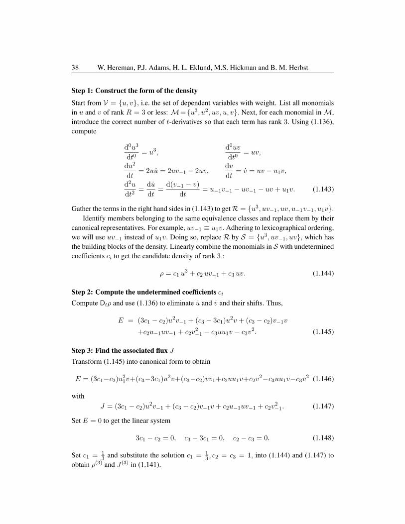
38 W. Hereman, P.J. Adams, H. L. Eklund, M.S. Hickman and B. M. Herbst
Step 1: Construct the form of the density
Start from V = {u, v}, i.e. the set of dependent variables with weight. List all monomialsin u and v of rank R = 3 or less: M={u3, u2, uv, u, v}. Next, for each monomial inM,introduce the correct number of t-derivatives so that each term has rank 3. Using (1.136),compute
d0u3
dt0= u3,
d0uv
dt0= uv,
du2
dt= 2uu = 2uv−1 − 2uv,
dvdt
= v = uv − u1v,
d2u
dt2=
dudt
=d(v−1 − v)
dt= u−1v−1 − uv−1 − uv + u1v. (1.143)
Gather the terms in the right hand sides in (1.143) to getR = {u3, uv−1, uv, u−1v−1, u1v}.Identify members belonging to the same equivalence classes and replace them by their
canonical representatives. For example, uv−1 ≡ u1v.Adhering to lexicographical ordering,we will use uv−1 instead of u1v. Doing so, replace R by S = {u3, uv−1, uv}, which hasthe building blocks of the density. Linearly combine the monomials in S with undeterminedcoefficients ci to get the candidate density of rank 3 :
ρ = c1 u3 + c2 uv−1 + c3 uv. (1.144)
Step 2: Compute the undetermined coefficients ciCompute Dtρ and use (1.136) to eliminate u and v and their shifts. Thus,
E = (3c1 − c2)u2v−1 + (c3 − 3c1)u2v + (c3 − c2)v−1v
+c2u−1uv−1 + c2v2−1 − c3uu1v − c3v2. (1.145)
Step 3: Find the associated flux JTransform (1.145) into canonical form to obtain
E = (3c1−c2)u21v+(c3−3c1)u2v+(c3−c2)vv1+c2uu1v+c2v2−c3uu1v−c3v2 (1.146)
withJ = (3c1 − c2)u2v−1 + (c3 − c2)v−1v + c2u−1uv−1 + c2v
2−1. (1.147)
Set E = 0 to get the linear system
3c1 − c2 = 0, c3 − 3c1 = 0, c2 − c3 = 0. (1.148)
Set c1 = 13 and substitute the solution c1 = 1
3 , c2 = c3 = 1, into (1.144) and (1.147) toobtain ρ(3) and J (3) in (1.141).

Direct Methods and Symbolic Software for Conservation Laws 39
1.11.3 The Ablowitz-Ladik Lattice
In [4–6], Ablowitz and Ladik derived and studied the following completely integrable dis-cretization of the nonlinear Schrodinger equation:
i un = un+1 − 2un + un−1 ± u∗nun(un+1 + un−1), (1.149)
where u∗n is the complex conjugate of un. We continue with (1.149) with the plus sign; thecase with the negative sign is analogous. Instead of splitting un into its real and imaginaryparts, we treat un and vn = u∗n as independent variables and augment (1.149) with itscomplex conjugate equation,
un = (un+1 − 2un + un−1) + unvn(un+1 + un−1),
vn = −(vn+1 − 2vn + vn−1)− unvn(vn+1 + vn−1), (1.150)
where i has been absorbed into a scale on t. Since vn = u∗n we have W (vn) = W (un).Neither equation in (1.150) is dilation invariant. To circumvent this problem we introducean auxiliary parameter α with weight, and replace (1.150) by
u = α(u1 − 2u+ u−1) + uv(u1 + u−1),
v = −α(v1 − 2v + v−1)− uv(v1 + v−1), (1.151)
presented in the simplified notation. Both equations in (1.151) are uniform in rank provided
W (u) + 1 = W (α) +W (u) = 2W (u) +W (v),
W (v) + 1 = W (α) +W (v) = 2W (v) +W (u), (1.152)
which holds when W (u) + W (v) = W (α) = 1. Since W (u) = W (v) we have W (u) =W (v) = 1
2 , and W (α) = 1, which expresses that (1.151) is invariant under the scalingsymmetry
(t, u, v, α)→ (λ−1t, λ12u, λ
12 v, λα). (1.153)
We give the conserved densities of (1.151) of ranks 2 through 4. Only the flux of rank 3associated to ρ(1) is shown. The others are omitted due to length.
ρ(1) = α(c1uv−1 + c2uv1), (1.154)
J (1) = −α [c1(αuv−2 − αu−1v−1 + u−1uv−2v−1)
+ c2(αuv − αu−1v1 − u−1uvv1)] , (1.155)
ρ(2) = α[c1(
12u
2v2−1 + uu1v−1v + αuv−2
)+c2
(12u
2v21 + uu1v1v2 + αuv2
)], (1.156)
ρ(3) = α(c1[
13u
3v3−1 + uu1v−1v(uv−1 + u1v + u2v1) + αuv−1(uv−2 + u1v−1)
+αuv(u1v−2 + u2v−1) + α2uv−3
]+ c2 [+uu1v1v2(uv1 + u1v2 + u2v3)]
+13u
3v31 + αuv2(uv1 + u1v2) + αuv3(u1v1 + u2v2) + α2uv3
]), (1.157)

40 W. Hereman, P.J. Adams, H. L. Eklund, M.S. Hickman and B. M. Herbst
where c1 and c2 are arbitrary constants. Our results confirm those in [6]. Since our methodis restricted to polynomial densities we cannot compute the density with a logarithmic term,
ρn = (u∗n(un−1 + un+1)− 2 ln(1 + unu∗n)) , (1.158)
which corresponds [3, 6] to the Hamiltonian of (1.149), viz. H = −i∑
n ρn.
1.11.4 Computation of a Conservation Law of the Ablowitz-Ladik Lattice
To make (1.150) scaling invariant we had to introduce an auxiliary parameter α. This com-plicates matters in two ways as we will show in this section. First, to compute rather simpleconserved densities, like ρ = uv−1 and ρ = uv1, we will have to select rank R = 2 forwhich the candidate density has twenty terms. However, eighteen of these terms eventuallydrop out. Second, conserved densities corresponding to lower ranks might appear in the re-sult. These lower-rank densities are easy to recognize for they are multiplied with arbitrarycoefficients ci. Consequently, when parameters with weight are introduced, the densitiescorresponding to distinct ranks are no longer linearly independent.
We compute ρ(1) of rank R = 2 in (1.154) with associated flux J (1) in (1.155). Notethat ρ(1) and J (1) cannot be computed with the steps below when R = 1.
Step 1: Construct the form of the density
Augment the set of dependent variables with the parameter α (with non-zero weight).Hence, V = {u, v, α}. Construct
M = {u, v, u2, uv, v2, αu, u3, αv, u2v, uv2, v3, αu2,
u4, αuv, u3v, αv2, u2v2, uv3, v4}, (1.159)
which contains all non-constant monomials of (chosen) rank 2 or less (without shifts). Aswith the previous examples, for each element inM add the right number of t−derivatives.Use (1.151) to evaluate the t−derivatives, gather the terms in the right hand sides, introducethe canonical representatives (based on lexicographical ordering), and remove duplicates toget
S = {αu2, u4, αuu1, αuv−1, αuv, u3v, u2u1v, u
2v−1v, αv2, u2v2, uu1v
2,
uv−1v2, uv3, v4, αuv1, uu
21v1, αvv1, u
2vv1, uv2v1, uu1v
21}. (1.160)
Linearly combine the monomials in S with undetermined coefficients ci to get the candidatedensity of rank 2:
ρ = c1 αu2 + c2 u
4 + c3 αuu1 + c4 αuv−1 + c5 αuv + c6 u3v + c7 u
2u1v
+c8 u2v−1v + c9 αv2 + c10 u
2v2 + c11 uu1v2 + c12 uv−1v
2 + c13 uv3
+c14 v4 + c15 αuv1 + c16 uu
21v1 + c17 αvv1 + c18 u
2vv1
+c19 uv2v1 + c20 uu1v
21. (1.161)

Direct Methods and Symbolic Software for Conservation Laws 41
Step 2: Compute the undetermined coefficients ciThe computations proceed as in the examples in Sections 1.9.2 and 1.11.2. Thus, computeDtρ and use (1.151) to eliminate u and v and their shifts. Next, bring the expression E intocanonical form to obtain the linear system for the undetermined coefficients ci.
Without showing the lengthy computations, one finds that all constants ci = 0, exceptc4 and c15 which are arbitrary. Substitute the coefficients into (1.161) to get ρ(1) in (1.154).
Step 3: Find the associated flux JThe associated flux comes for free when E is transformed into canonical form. Alterna-tively, one could apply the homotopy approach for multiple dependent variables [51, 54] tocompute the flux. In either case, one gets J (1) in (1.155).
1.11.5 A “Divide and Conquer” Strategy
It should be clear from the example in Section 1.11.4 that our method is not efficient if thedensities are not of the form (1.111)-(1.114) for the KvM lattice and (1.139)-(1.142) for theToda lattice. Indeed, the densities for the AL lattice in (1.154)-(1.157) are quite different instructure. Therefore, in [33], Eklund presented alternate strategies to deal more efficientlywith DDEs, in particular with those involving weighted parameters such as (1.151).
A first alternative is to work with multiple scales by setting either W (Dt) = 0 orW (Dt) = 1, the latter choice is what we have used thus far. A second possibility is toleave W (Dt) unspecified and, if needed, introduce extra parameters with weight into theDDE.
Let us explore these ideas for the AL lattice (1.151), which we therefore replace by
u = αβ(u1 − 2u+ u−1) + βuv(u1 + u−1),
v = −αβ(v1 − 2v + v−1)− βuv(v1 + v−1), (1.162)
where β is a second auxiliary parameter with weight. Requiring uniformity in rank leads to
W (u) +W (Dt) = W (α) +W (β) +W (u) = W (β) + 2W (u) +W (v),
W (v) +W (Dt) = W (α) +W (β) +W (v) = W (β) + 2W (v) +W (u),(1.163)
which are satisfied when W (α) = W (u) +W (v) and W (Dt) = W (u) +W (v) +W (β).Therefore, we can set W (Dt) = a,W (u) = b, and W (β) = c with a, b, c rational numbersso that W (v) = a− b− c and W (α) = a− c are strictly positive. Thus (1.162) is dilationinvariant under a three-parameter family of scaling symmetries,
(t, u, v, α, β)→ (λ−at, λbu, λa−b−cv, λa−cα, λcβ). (1.164)
Scaling symmetry (1.153) corresponds to the case where a = 1, b = 12 , and c = 0, more
precisely, β = 1. The fact that (1.162) is invariant under multiple scales is advantageous.

42 W. Hereman, P.J. Adams, H. L. Eklund, M.S. Hickman and B. M. Herbst
Indeed, one can use the invariance under one scale to construct a candidate density and,subsequently, use additional scale(s) to split ρ into smaller densities. This “divide and con-quer” strategy drastically reduces the complexity of the computations. The use of multiplescales has proven to be successful in the computation of conservation laws for PDEs withmore than one space variable [51].
Table 1.4: Candidate densities for the Ablowitz-Ladik lattice (1.162).
i Rank Candidate ρi Final ρi Final Ji1 a+ 2b− c c1αu
2 + c3αuu1 + c6u3v 0 0
+c7u2u1v + c16uu21v1
2 4b c2u4 0 0
3 2(a− c) c4αuv−1 + c5αuv + c8u2v−1v c4αuv−1 J (1) in (1.155)
+c10u2v2 + c11uu1v
2 + c15αuv1 +c15αuv1+c18u
2vv1 + c20uu1v21
4 3a− 2b− 3c c9αv2 + c12uv−1v
2 + c13uv3 0 0
+c17αvv1 + c19uv2v1
5 4(a− b− c) c14v4 0 0
Candidate density (1.161) is uniform of rank 2 under (1.153) but can be split into smallerpieces, ρi, using (1.164), even without specifying values for a, b, and c. Indeed, as shown inTable 1.4, ρ in (1.161) can be split into ρ1 through ρ5 of distinct ranks under (1.164). Steps2 and 3 of the algorithm are then carried out for each of these ρi, (i = 1, · · · , 5) separately.As shown in the table, all but one density lead to a trivial result. The longest density, ρ3,
with 8 terms, leads to ρ(1) and J (1) in (1.154) and (1.155), respectively.
1.12 A New Method to Compute Conservation Laws of Nonlin-ear DDEs
In the continuous case, the total derivative Dx has weight one. Consequently, any densityis bounded with respect to the order in x. For example, as shown in Section 1.3.2 for theKdV case, the candidate density ρ of rank 6 in (1.18) is of first order (after removing thesecond and fourth order terms.) Obviously, a density of rank 6 could never have leadingorder terms of fifth or higher order in x because the rank of such terms would exceed 6.
In the discrete case, however, the shift operator D has no weight. Thus, any shift Dku =uk of a dependent variable u has the same weight as that dependent variable. Simply put,W (uk) = W (u) for any integer k. Consequently, using the total derivative Dt as a toolto construct a (candidate) density has a major shortcoming: the density may lack terms

Direct Methods and Symbolic Software for Conservation Laws 43
involving sufficiently high shifts of the variables. As shown in Section 1.9.2 for the KvMlattice, the candidate density ρ of rank 3 in (1.118) has leading order term uu1u2, i.e. theterm with the highest shift (2 in this example). It is a priori not excluded that ρ mighthave terms involving higher shifts. For example, uu1u3 has rank 3 and so do infinitelymany other cubic terms. Note that for this example we constructed ρ starting from powersof u, viz. u3, u2, u; and, by repeated differentiation, worked our way “down” towards theleading order term uu1u2. In this section we outline the key features of a new method whichgoes in the opposite direction: (i) first compute the leading order term and subsequently (ii)compute the terms involving lower shifts. In step (ii) only the necessary terms are computed,nothing more, nothing less. This method is fast and powerful for it circumvents the use ofthe dilation invariance and the method of undetermined coefficients. More importantly, thenew method is not restricted to densities and fluxes of polynomial form.
1.12.1 Leading Order Analysis
Consider a density, ρ, that depends on q shifts. Since Dq ρ is also a density, we may, withoutloss of generality, assume that ρ has canonical form ρ(u, u1, . . . , uq) with ∂2ρ
∂u ∂uq6= 0.
In [55], Hickman derived necessary conditions on this leading term (which, in the systemcase, is a matrix). First all terms in the candidate density ρ that contribute directly to theflux are removed. Rather than applying the Euler operator on the remaining terms in ρ, thenecessary condition [57],
∂2g
∂u ∂uq= 0, (1.165)
for g to be a total difference is applied to obtain a system of equations for the terms that de-pend on the maximal shift, uq, in ρ. This system is rewritten as a matrix equation. Solutionsto this system will give us the form of the leading term in ρ.
We apply a splitting of the identity operator,
I = (D− I + I) D−1 = ∆ D−1 + D−1, (1.166)
to the part, ρ∗, of the candidate ρ that is independent of the variables with the lowest ordershift. The first term ∆ D−1 ρ∗ contributes to the flux while the second term D−1 ρ∗ has astrictly lower shift than ρ∗. Applying this split repeatedly we get
I = (Dk − I + I) D−k = ∆(Dk−1 + Dk−2 + · · ·+ D + I
)D−k + D−k, (1.167)
where, again, the first term contributes to the flux and the remainder has strictly lower shift.This decomposition is repeatedly applied to terms that do not involve the lowest order
shifted variables. Any terms that remain will involve the lowest order shifted variable.These terms yield the constraints on the undetermined coefficients or unknown functions in

44 W. Hereman, P.J. Adams, H. L. Eklund, M.S. Hickman and B. M. Herbst
the density ρ. As shown in [55], the result of this split is that ρ is a density if and only if
σ = Dl
(F∂
∂u
) l∑j=0
Djρ+q∑
j=l+1
Dj
(F∂
∂u
)ρ (1.168)
is a total difference, where the operator
F∂
∂u=∑α
Fα∂
∂uα(1.169)
involves a summation over the components in the system of DDEs. As before, in the exam-ples we will use u, v, w, etc. to denote the dependent variables uα.
Now, σ depends on the shifted variables u, . . . , uq+L where L = max (l, m). Forq > L, (1.165) gives
∂2σ
∂u ∂uq+L= DL
(∂2ρ
∂u ∂uq
∂F∂u−L
)+ Dq
(∂F∂uL
)T ∂2ρ
∂u ∂uq= 0, (1.170)
where T stands for transpose. The system case is treated in detail in [55]. For brevity, wecontinue with the scalar case. Let
λ =∂F
∂u−L, µ =
∂F
∂uL, (1.171)
then the leading term will satisfy
S ∂2ρ
∂u ∂uq= 0, (1.172)
with S = DL λDL + Dq µ. We immediately see that if l 6= m then either λ or µ is zero and(1.172) has no non-trivial solutions. Let q = pL+ r with p and r integers, 0 ≤ r < L, and
c =
(p−1∏k=1
DkLλ
)DpLζ. (1.173)
Then
S c =p−1∏k=1
DkLλDpL(λDLζ + ζ Drµ
). (1.174)
Thus c 6= 0 lies in the kernel of S if and only if
λDLζ + ζ Drµ = 0 (1.175)
has a non-zero solution ζ. Suppose (1.175) has two non-zero solutions, say, ζ1 and ζ2. Then,
ζ2ζ1
= DL
(ζ2ζ1
). (1.176)

Direct Methods and Symbolic Software for Conservation Laws 45
So, since L 6= 0, ζ2 = aζ1 for some constant a. Therefore, the kernel of S is, at most, onedimensional. This implies that a scalar DDE can have, at most, one conserved density thatdepends on q shifts for q > L. The leading term, ρ, will satisfy
∂2ρ
∂u ∂uq= c, (1.177)
which, upon integration, yields
ρ =∫∫
c du duq. (1.178)
The density (if it exists) may now be computed by a “split and shift” strategy on this leadingterm. Starting with ρ = ρ. the objective is to successively compute the terms (of lowershift!) that must be added to ρ until Dt ρ ≡ 0. First, Dt ρ is computed and evaluated on theDDE. Next, all terms are shifted so that the resulting expression depends on u (and not onlower shifts of u). Then the leading terms, ξ, in Dt ρ are isolated. Last, we solve
Dt ρ(1) = ξ + terms of lower shift. (1.179)
If (1.179) has no solution then a density with q shifts does not exist. On the other hand, if(1.179) has a solution, the “correction” term ρ(1) is then subtracted from ρ and we recom-pute Dt ρ. By construction, the highest shift that occurs in the result will now be lower thanbefore and we repeat the entire procedure to obtain a new correction term ρ(2). After a finitenumber of steps, we will either find an that the correction term does not exist (and so thedensity does not exist) or we will obtain Dt ρ ≡ 0 and ρ will be a density.
This algorithm has been coded [56] in Maple. Further details and worked exampleswill be presented in [58]. For now, we illustrate the algorithm with a simple example.
1.12.2 A“Modified” Volterra Lattice
Consider the DDE,u = u2 (u2 − u−2), (1.180)
which is related to the well-known modified Volterra Lattice [11]. Here L = 2 and, using(1.171),
λ =∂F
∂u−2= − u2, µ =
∂F
∂u2= u2. (1.181)
Thus, the condition (1.175) for a non-trivial density becomes ζ u2r = u2 D2ζ for r = 0, 1.
For r = 0, we have ζ = D2ζ and so we may choose ζ = 1. For r = 1, we have ζ u21 =
u2 D2ζ, which has no non-zero solutions. Thus, densities only exist for r = 0. Sinceq = pL = 2p, with p integer, we conclude that q must be even. In these cases the leadingterm will satisfy
∂2ρ
∂u ∂uq= c =
(p−1∏k=1
u2k
)= uu2 · · · uq−2. (1.182)

46 W. Hereman, P.J. Adams, H. L. Eklund, M.S. Hickman and B. M. Herbst
Therefore, after scaling to remove constants, the leading term is ρ = u2 u2 · · · uq−2 uq.
For example, let us compute the density that depends on q = 4 shifts. We set ρ = ρ =u2 u2 u4. Using (1.180),
Dt ρ = u2u22u4 (u2 − u−2) + 2uu3
2 u4 (u4 − u) + uu22 u
24 (u6 − u2)
≡ uu32 u
24 − u2 u3
2 u4. (1.183)
The highest shift is u4 and so the leading terms are
ξ = uu32 u
24 − u2 u2
3 u4. (1.184)
Note that the terms in u6 must cancel by the construction of ρ. Next, we note that u4 as aleading term must arise as either u2 = u2
2 (u4 − u) or
u2 u = u2 u2 (u2 − u−2) ≡ u2 u2
2 − uu22 u4. (1.185)
The quadratic term must arise from (1.185) (as we have already determined all terms thatinvolve u4, so, we cannot have a quadratic term given by u4u2). Now, we solve (1.179) toget
ρ(1) = −12u2 u2
2 + · · · . (1.186)
Indeed,
Dt
(−1
2 u2 u2
2
)= −uu2
2 u− u2 u2 u2
≡ uu32 u
24 − u2 u3
2 u4 + lower shift terms
= ξ + lower shift terms, (1.187)
with ξ in (1.184). Thus, we update ρ = u2u2u4 by subtracting ρ(1). This yields,
ρ = u2 u2 u4 +12u2 u2
2. (1.188)
We readily verify that Dt ρ ≡ 0 and, thus, ρ in (1.188) is the unique density of (1.180) thatdepends on 4 shifts.
1.13 The Gardner Lattice
In this section we consider the DDE described in [91],
u =(1 + αh2u+ βh2u2
){ 1h3
(12u−2 − u−1 + u1 −
12u2
)+α
2h[u−1u−2 + u2
−1 + u(u−1 − u1)− u21 − u1u2
]+
β
2h[u2−1(u−2 + u)− u2
1(u+ u2)]}
, (1.189)

Direct Methods and Symbolic Software for Conservation Laws 47
which is a completely integrable discretization of the Gardner equation,
ut + 6αuux + 6βu2ux + u3x = 0. (1.190)
Therefore, we call (1.189) the Gardner lattice. Note that (1.190) is a combination of theKdV equation (β = 0) and the mKdV equation (α = 0). Consequently, (1.189) includesthe completely integrable discretizations of the KdV and mKdV equations as special cases.
1.13.1 Derivation of the Gardner Lattice
Based on work by Taha [91], we outline the derivation of the Gardner lattice from a dis-cretized version [4] of the eigenvalue problem of Zakharov and Shabat. Consider the dis-crete system [1, 7],
V1,n+1 = zV1,n +Qn(t)V2,n, V2,n+1 =1zV2,n +Rn(t)V1,n, (1.191)
V1,n = An(z)V1,n +Bn(z)V2,n, V2,n = Cn(z)V1,n +Dn(z)V2,n, (1.192)
where, in general, the coefficients An through Dn depend on the potentials, Rn and Qn.The eigenvalue z is assumed to be time-independent.
Step 1: Expressing the compatibility conditions, Vi,n+1 = DVi,n, for i = 1, 2, and equatingthe coefficients of V1,n and V2,n, we get [7]
CnQn −Bn+1Rn = z(An+1 −An),
BnRn − Cn+1Qn =1z
(Dn+1 −Dn), (1.193)
Qn +DnQn −An+1Qn =1zBn+1 − zBn,
Rn +AnRn −Dn+1Rn =1zCn+1 − zCn. (1.194)
Step 2: Substituting the expansions [91],
An =2∑
j=−2
z2jA(2j)n , Dn =
2∑j=−2
z2jD(2j)n , (1.195)
Bn =2∑
j=−1
z2j−1B(2j−1)n , Cn =
2∑j=−1
z2j−1C(2j−1)n , (1.196)
into (1.193) and (1.194) and setting the coefficients of like powers of z equal to zero, weobtain a system of twenty equations for the eighteen unknowns functions A(2j)
n , D(2j)n with

48 W. Hereman, P.J. Adams, H. L. Eklund, M.S. Hickman and B. M. Herbst
j = −2,−1, 0, 1, 2; and B(2j−1)n , C
(2j−1)n with j = −1, 0, 1, 2. The simplest equations
arise from the coefficients of the terms in z±5 and z±4 :
A(4)n+1 −A
(4)n = 0, D
(−4)n+1 −D
(−4)n = 0, (1.197)
Qn(D(4)n −A
(4)n+1) +B(3)
n = 0, Rn(A(−4)n −D(−4)
n+1 ) + C(−3)n = 0, (1.198)
Qn(D(−4)n −A(−4)
n+1 )−B(−3)n+1 = 0, Rn(A(4)
n −D(4)n+1)− C(3)
n+1 = 0. (1.199)
Step 3: We outline the solution process which follows the strategy in [7, Section 2.2a].From (1.197), we conclude that A(4)
n and D(−4)n are independent of n. Hence, A(4)
n = A(4)
and D(−4)n = D(−4) are constants. The tilde will remind us that we are dealing with
constants. Solving (1.198) and (1.199), we get
B(3)n = (A(4) −D(4)
n )Qn, C(−3)n = (D(−4) −A(−4)
n )Rn, (1.200)
B(−3)n = (D(−4) −A(−4)
n )Qn−1, C(3)n = (A(4) −D(4)
n )Rn−1. (1.201)
Substituting these results into two of the equations coming from z±3, we find that A(−4)n =
A(−4) and D(4)n = D(4) are constants. From equations corresponding to z±3, z±1, we
obtain
∆A(2)n = A
(2)n+1 −A
(2)n = α(QnRn−1 −Qn+1Rn), (1.202)
∆D(−2)n = D
(−2)n+1 −D
(−2)n = β(RnQn−1 −Rn+1Qn), (1.203)
∆A(−2)n = A
(−2)n+1 −A
(−2)n = β(QnRn+1 −Qn−1Rn), (1.204)
∆D(2)n = D
(2)n+1 −D
(2)n = α(RnQn+1 −Rn−1Qn), (1.205)
where α = A(4) − D(4) and β = D(−4) − A(−4). Equations (1.202)-(1.205) are satisfiedfor
A(2)n = A(2) − αQnRn−1, D(−2)
n = D(−2) − βRnQn−1, (1.206)
A(−2)n = A(−2) + βQn−1Rn, D(2)
n = D(2) + αRn−1Qn, (1.207)
where A(2), D(−2) and A(−2), D(2) are constants. Next, we solve equations (from the termsin z±2) for B(±1)
n and C(±1)n , yielding
B(1)n = δQn + αQn+1 − αQn(Qn+1Rn +QnRn−1), (1.208)
C(−1)n = γRn + βRn+1 − βRn(Rn+1Qn +RnQn−1), (1.209)
B(−1)n = γQn−1 + βQn−2 − βQn−1(Rn−1Qn−2 +RnQn−1), (1.210)
C(1)n = δRn−1 + αRn−2 − αRn−1(Qn−1Rn−2 +QnRn−1), (1.211)
where δ = A(2) − D(2) and γ = D(−2) − A(−2). Next, we solve equations coming fromz±1, which involve ∆A(0)
n and ∆D(0)n . These equations, which are similar in structure to

Direct Methods and Symbolic Software for Conservation Laws 49
(1.202)-(1.205), yield
A(0)n = α (−Qn+1Rn−1 −QnRn−2 +QnQn+1Rn−1Rn
+Qn−1QnRn−2Rn−1 +Q2nR
2n−1
)+ A(0) − δRn−1Qn, (1.212)
D(0)n = β (−Rn+1Qn−1 −RnQn−2 +RnRn+1Qn−1Qn
+Rn−1RnQn−2Qn−1 +R2nQ
2n−1
)+ D(0) − γQn−1Rn, (1.213)
where A(0) and D(0) are constants. All the difference equations for the unknown coeffi-cients are now satisfied. We are left with the two DDEs (coming from the terms in z0),
Qn − κQn + (1−QnRn)[−αQn+2 − δQn+1 + γQn−1 + βQn−2
+αQn+1(Qn+2Rn+1 +Qn+1Rn)− βQn−1(Qn−2Rn−1 +Qn−1Rn)
+αQnQn+1Rn−1 − βQnQn−1Rn+1
]= 0, (1.214)
Rn + κRn + (1−RnQn)[−βRn+2 − γRn+1 + δRn−1 + αRn−2
+βRn+1(Rn+2Qn+1 +Rn+1Qn)− αRn−1(Rn−2Qn−1 +Rn−1Qn)
+βRnRn+1Qn−1 − αRnRn−1Qn+1
]= 0, (1.215)
where κ = A(0) − D(0).
Step 4: The terms −κQn in (1.214) and κRn in (1.215) could be removed with a suitabletransformation. Accomplishing the same, we set κ = 0. Next, we substitute
Qn = un, Rn = −h2(α+ βun), (1.216)
into (1.214) and (1.215). Next, we set β = α and γ = δ to remove all constant terms.Doing so, (1.214) and (1.215) collapse into a single DDE,
un + (1 + αh2un + βh2u2n){α(un−2 − un+2) + δ(un−1 − un+1)
+ααh2(un−2un−1 + u2n−1 +un(un−1−un+1)−u2
n+1 −un+1un+2)
+βαh2(u2n−1(un−2+un)−u2
n+1(un+un+2))}
= 0, (1.217)
Step 5: To fix the scale on t, as well as the constants α, β, and δ, we consider the limitof (1.217) for h → 0. Using, limh→0 un(t) = u(x, t), limh→0 un(t) = ut(x, t), andsubstituting
limh→0
un+m(t) = u(x, t) +mhux(x, t) +12
(mh)2u2x(x, t)
+16
(mh)3u3x(x, t) + · · · , (1.218)

50 W. Hereman, P.J. Adams, H. L. Eklund, M.S. Hickman and B. M. Herbst
into (1.217), we obtain
ut − 2h(δ + 2α)ux − 2h3(δ + 8α)(αuux + βu2ux + 1
6u3x
)+O(h5) = 0. (1.219)
The term in h disappears when δ = −2α. Substituting α = −12 , δ = 1, into (1.217) and
(1.219), we get
u =(1 + αh2u+ βh2u2
){12u−2 − u−1 + u1 −
12u2
+12αh2
[u−1u−2 + u2
−1 + u(u−1 − u1)− u21 − u1u2
]+
12βh2
[u2−1(u−2 + u)− u2
1(u+ u2)]}
, (1.220)
andut + h3(6αuux + 6βu2ux + u3x) = 0, (1.221)
where the O(h5) terms were ignored. Using a scale, t→ h3t, we get (1.189) and (1.190).
Remarks. Step 2 is well suited for a CAS. Solving the system, as outlined in Step 3, isa challenging task, in particular, if attempted with pen and paper. The system consistsof two DDEs and eighteen difference equations. None of the CAS has a build-in solverfor such mixed systems. A fully automated solution is therefore impossible. We useda feedback mechanism which mimics what one would do by hand: Solve the simplestdifference equations; enter that partial solution; let CAS simplify the entire system; repeatthe process until all difference equations are satisfied and the two DDEs are simplified asfar as possible. Continuing with (1.214) and (1.215), steps 4 and 5 were straightforwardto implement. The five steps have been implemented in Mathematica [50]. Startingfrom (1.191), the code generates the Gardner lattice (1.220). The code could be modifiedto assist in the derivation of other completely integrable DDEs, such as discrete versions ofthe nonlinear Schrodinger and sine-Gordon equations.
1.13.2 Dilation Invariance of the Gardner Lattice
Since (1.189) is not uniform in rank we must introduce auxiliary parameters with weight.This can be done in several ways. One of the possibilities is to replace (1.189) by
u =(γ + αu+ βu2
){γ
(12u−2 − u−1 + u1 −
12u2
)+α
2[u−1u−2 + u2
−1 + u(u−1 − u1)− u21 − u1u2
]+β
2[u2−1(u−2 + u)− u2
1(u+ u2)]}
, (1.222)
where we have set h = 1 (by scaling) and introduced a parameter γ.

Direct Methods and Symbolic Software for Conservation Laws 51
Expressing uniformity of rank, setting W (Dt) = 1, and solving the linear system forthe weights, one finds that W (u) = W (α) = 1
4 , W (β) = 0, and W (γ) = 12 . So, we do not
need a scale on β and (1.222) is invariant under the scaling symmetry
(t, u, α, γ)→ (λ−1t, λ14u, λ
14α, λ
12γ). (1.223)
For β = 0, (1.222) reduces to
u = (γ + αu){γ
(12u−2 − u−1 + u1 −
12u2
)+α
2[u−1u−2 + u2
−1 + u(u−1 − u1)− u21 − u1u2
]}, (1.224)
which is a completely integrable discretization of the KdV equation, ut+6αuux+u3x = 0.Computing the weights, one can set W (α) = 0, which leads to W (u) = W (γ) = 1
2 . So,
(1.224) is invariant under the scaling symmetry (t, u, γ) → (λ−1t, λ12u, λ
12γ). For α = 0,
(1.222) reduces to
u =(γ + βu2
){γ
(12u−2 − u−1 + u1 −
12u2
)+β
2[u2−1(u−2 + u)− u2
1(u+ u2)]}
, (1.225)
which is a completely integrable discretization of the mKdV equation, ut+6βu2ux+u3x =0. In this case, one can set W (β) = 0. Then W (u) = 1
4 and W (γ) = 12 . Thus, (1.225) is
invariant under the scaling symmetry (t, u, γ)→ (λ−1t, λ14u, λ
12γ).
1.13.3 Conservation Laws of the Gardner Lattice
One can either apply the method of Section 1.12 directly to (1.189) or, alternatively, applyto (1.222) the technique based on dilation invariance outlined in Sections 1.9.2, 1.11.2,and 1.11.4. In particular, one can use the “divide and conquer” strategy of Section 1.11.5to split candidate densities into smaller pieces. Computational details can be found in [33]The results below were computed [58] with the method in Section 1.12. For q = 0 shiftsthere are two (non-polynomial) density-flux pairs:
ρ(0)1 = ln (1 + αh2 u+ βh2 u2), (1.226)
J(0)1 = −1
2
{αh
(u−2 − u−1 − u+ u1) +β
h(2u−2u− 4u−1u+ 2u−1u1)
+α2h(u−1(u−2 + u−1 + u) + u(u−1 + u+ u1)
)+ αβ h
(u2−1u−2
+2u−2u−1u+ 3u2−1u+ 3u−1u
2 + 2u−1uu1 + u2u1
)+2β2 hu−1u
(u−2u−1 + u−1u+ uu1
)}, (1.227)

52 W. Hereman, P.J. Adams, H. L. Eklund, M.S. Hickman and B. M. Herbst
and
ρ(0)2 = arctanh
(h(α+ 2βu)√α2 h2 − 4β
), (1.228)
J(0)2 =
14
√α2h2 − 4β
{1h2 (2u−1 − u−2 − 2u1 + u2)
+α(u−2u−1 + u2
−1 + 2u−1u+ u2 + uu1
)+β(u2−1(u−2 + u) + u2(u−1 + u1)
)}. (1.229)
The next two (of infinitely many polynomial) densities are
ρ(1) = uu1 +α
βu, (1.230)
ρ(2) = uu2
(1 + αh2u1 + βh2u2
1
)+ αh2uu1(u+ u1)
+12βh2u2u2
1 +α
β(1− α2
βh2)u+
α2
2βh2u2, (1.231)
where the associated fluxes have been omitted due to length.
Special Cases.
We consider two important special cases. The first few densities for (1.189) with β = 0 are:
ρ(0)1 = ln (1 + αh2u), ρ(0)
2 = u, (1.232)
ρ(1) = 12 u
2 + uu1,
ρ(2) = uu2(1 + αh2u1) + αh2u(u21 + uu1 + 1
3 u2). (1.233)
The first few densities for (1.189) with α = 0 are
ρ(0)1 = ln (1 + βh2u2), ρ
(0)2 = arctan (
√βhu), (1.234)
ρ(1) = uu1, ρ(2) = uu2(1 + βh2u21) + 1
2 βh2u2u2
1. (1.235)
1.14 Additional Examples of Nonlinear DDEs
1.14.1 The Bogoyavlenskii Lattice
The Bogoyavlenskii lattice [21] and [90, Eq. (17.1.2)],
u = u
p∏j=1
uj −p∏j=1
u−j
, (1.236)
is a generalization of the KvM lattice (1.110). For p = 2, lattice (1.236) becomes
u = u(u1u2 − u−1u−2), (1.237)

Direct Methods and Symbolic Software for Conservation Laws 53
which is invariant under the following scaling symmetry
(t, u)→ (λ−1t, λ12u). (1.238)
Lattice (1.237) has the following density-flux pairs (of infinitely many):
ρ(0) = lnu, J (0) = −(u−1u−2 + u−1u+ uu1), (1.239)
ρ(1) = u, J (1) = −uu−1(u−2 + u1), (1.240)
ρ(2) = uu1, J (2) = −u−1uu1(u−2 + u+ u2), (1.241)
ρ(3) = uu1(12uu1 + u1u2 + u2u3), (1.242)
J (3) = −u−1uu1(u−2uu1 + u2u1 + u−2u1u2 + 2uu1u2 + u1u22
+u−2u2u3 + uu2u3 + u22u3 + u2u3u4). (1.243)
For (1.237), we also computed the densities ρ(4) through ρ(9). Every time the rank increasesby one, the number of terms in the density increases by a factor three. For example, ρ(9)
has 2187 terms and the highest shift is 15.
1.14.2 The Belov-Chaltikian Lattice
The Belov-Chaltikian lattice [18, Eq. (12)],
u = u(u1 − u−1) + v−1 − v, v = v(u2 − u−1), (1.244)
in invariant under the scaling symmetry
(t, u, v)→ (λ−1t, λu, λ2v). (1.245)
The first few density-flux pairs (of infinitely many) are
ρ(1) = u, J (1) = −u−1u+ v−1, (1.246)
ρ(2) = 12u
2 + uu1 − v,J (2) = −u−1u
2 − u−1uu1 + uv−1 + u1v−1 + u−1v, (1.247)
ρ(3) = u(13u
2 + uu1 + u21 + u1u2 − v−2 − v−1 − v − v1), (1.248)
where J (3) has been omitted due to length. Our results match these in [84].
1.14.3 The Blaszak-Marciniak Lattices
In [19], Blaszak and Marciniak used the R matrix approach to derive families of integrablelattices involving three and four fields. Below we consider two cases involving three fields.Examples based on four fields could be dealt with in a similar fashion [113].

54 W. Hereman, P.J. Adams, H. L. Eklund, M.S. Hickman and B. M. Herbst
The Blaszak-Marciniak three field lattice I [84, Eq. (2)],
u = w1 − w−1, v = u−1w−1 − uw, w = w(v − v1), (1.249)
is invariant under the scaling symmetry
(t, u, v, w)→ (λ−1t, λ12u, λv, λ
32w). (1.250)
We computed the following density-flux pairs of (1.249), which is a completely integrablelattice:
ρ(0) = lnw, J (0) = v, (1.251)
ρ(1) = u, J (1) = −w−1 − w, (1.252)
ρ(2) = v, J (2) = u−1w−1, (1.253)
ρ(3) = 12v
2 + uw, J (3) = u−1vw−1 − w−1w, (1.254)
ρ(4) = 13v
3 + uvw + uv1w − ww1, (1.255)
J (4) = w−1(u−1v2 + u−1uw − vw − v1w). (1.256)
Our results confirm those in [84] and [112]. The Blaszak-Marciniak three field lattice II[112, Eq. (1.4)],
u = v1 − v + u(w−1 − w), v = v(w−2 − w), w = u1 − u, (1.257)
is invariant under the scaling symmetry
(t, u, v, w)→ (λ−1t, λ2u, λ3v, λw). (1.258)
The first few density-flux pairs for (1.257), which is completely integrable, are
ρ(1) = w, J (1) = −u, (1.259)
ρ(2) = 12w
2 − u, J (2) = v − uw−1, (1.260)
ρ(3) = 13w
3 + v − uw−1 − uw, J (3) = u−1u+ vw−2 + vw−1 − uw2−1, (1.261)
ρ(4) = 14w
4 + 12u
2 + uu1 + vw−2 + vw−1 − uw2−1
+vw − uw−1w − uw2, (1.262)
J (4) = −u−2v − uv − u−1v1 + vw2−2 + 2u−1uw−1
+vw−2w−1 + vw2−1 − uw3
−1 + u−1uw. (1.263)
Our results agree with those in [84] and [112].
1.15 Software to Compute Conservation Laws for PDEs andDDEs
We first discuss our packages for conservation laws of PDEs and DDEs, followed by a briefsummary of symbolic codes developed by other researchers.

Direct Methods and Symbolic Software for Conservation Laws 55
1.15.1 Our Mathematica and Maple Software
The package TransPDEDensityFlux.m [9] , automates the computation of conserva-tion laws of nonlinear PDEs in (1 + 1) dimensions. In addition to polynomial PDEs, thesoftware can handle PDEs with transcendental nonlinearities. The results in Sections 1.3and 1.5 were computed with TransPDEDensityFlux.m and cross-checked with thenewest version of condens.m, introduced in [38]. We used TransPDEDensityFlux.mto compute the density-flux pairs for the examples in Sections 1.6 and 1.7. Details aboutthe algorithm and a discussion of implementation issues can be found in [8].
The code DDEDensityFlux.m [34] was used to compute the conservation laws inSections 1.9 and 1.11. The results were cross-checked with the latest version of diffdens.m, featured in [39]. Using multiple scales, the efficiency of DDEDensityFlux.mwas dras-tically improved. Nonetheless, the algorithms [33] within DDEDensityFlux.m are im-practical for finding densities and fluxes of high rank. Therefore, we used the new Maplelibrary discrete [56] to compute the results in Sections 1.13 and 1.14.
Some of the features of earlier versions of condens.m and diffdens.m were com-bined into the InvariantsSymmetries.m [39,41], which allows one to compute gen-eralized symmetries as well as conserved densities (but no fluxes). InvariantsSymme-tries.m is available from MathSource, the Mathematica program bank of WolframResearch, Inc.
Our Mathematica packages and notebooks are available at [48] and Hickman’s Maplecode is available at [56]. Our Mathematica codes for the continuous and discrete Eulerand homotopy operators in one dimension are available at [49]. We are currently designinga comprehensive package to compute conservation laws of PDEs in multiple space dimen-sions [45, 51, 83].
Our codes have been used in a variety of research projects. For example, condens.m[38] was used by Sakovich and Tsuchida [85, 95] to compute conservation laws of non-linear Schrodinger equations. In [84], Sahadevan and Khousalya use the algorithms ofdiffdens.m [42] and InvariantsSymmetries.m [39, 41] to compute conserveddensities of the Belov-Chaltikian and Blaszak-Marciniak lattices. Ergenc and Karasozen[35] used our software in the design of Poisson integrators for Volterra lattices.
1.15.2 Software Packages of Other Researchers
Our Mathematica code for conservation laws of PDEs has been “translated” [108–110]into a Maple package, called CONSLAW , which only handles PDEs in (1 + 1) dimensions.Based on the concept of dilation invariance and the method of undetermined coefficients,similar software was developed by Deconinck and Nivala [27] and Yang et al. [107]. Ouralgorithms [38, 42] for DDEs have been adapted to fully-discretized equations [36, 37].
There are several algorithms (see e.g. [101]) to symbolically compute conservation lawsof nonlinear PDEs but few have been fully implemented in CAS. Wolf’s package ConLaw

56 W. Hereman, P.J. Adams, H. L. Eklund, M.S. Hickman and B. M. Herbst
[101, 102, 106] computes first integrals of ODEs and conservation laws of PDEs. ConLawuses the REDUCE package CRACK [103–105], which contains tools to solve overdeterminedsystems of PDEs. Wolf’s application packages heavily rely on the capabilities of CRACK,which took years to develop and perfect. Unfortunately, no such package is available inMathematica.
A common approach is to use the link between conservation laws and symmetries asstated in Noether’s theorem [15, 66, 81]. Among the newest software based on that ap-proach is the Maple code GeM [25] by Cheviakov [23, 24], which allows one to computeconservation laws of systems of ODEs and PDEs based on the knowledge of generalizedsymmetries. However, the computation of such symmetries [47] is as difficult a task as thedirect computation of conservation laws for it requires solving systems of overdeterminedPDEs with, e.g., the Rif package [47, 100]. Some methods circumvent the existence of avariational principle (required by Noether’s theorem) [12,20,101,106] but they still rely onsoftware to solve ODEs or PDEs.
The package DE APPLS [16, 77] also offers commands for constructing conservationlaws from (variational) symmetries by Noether’s theorem, but the computation is not fullyautomated. Likewise, the package Noether [43] in Maple allows one to compute conser-vation laws from infinitesimal symmetry generators corresponding to (simple) Lagrangians.
Based on the formal symmetry approach, Sokolov and Shabat [89], Mikhailov et al.[74, 75], and Adler et al. [10] classified completely integrable PDEs and DDEs in (1 + 1)dimensions. Unfortunately, the software used (see [38]) in the classification is obsolete.
For completeness, we also mention the packages Jets by Marvan [73] and Vessiotby Anderson [16, 77]. Both are general purpose suites of Maple packages for computa-tions on jet spaces. The commands within Jets and Vessiot use differential forms andadvanced concepts from differential geometry. By avoiding differential forms, our codeswere readily adaptable to nonlinear DDEs (not covered in Jets and Vessiot).
Finally, Deconinck and Nivala [26] developed Maple software for the continuous anddiscrete homotopy operators. Their code is available at [28].
1.16 Summary
We presented methods to symbolically compute conservation laws of nonlinear polynomialand transcendental systems of PDEs in (1 + 1) dimensions and polynomial DDEs in onediscrete variable.
The first part of this chapter dealt with nonlinear PDEs for which we showed the com-putation of densities and fluxes in detail. Using the dilation invariance of the given PDE,candidate polynomial densities are constructed as linear combinations with undeterminedcoefficients of scaling invariant building blocks. For polynomial PDEs, the undeterminedcoefficients are constants which must satisfy a linear system of algebraic equations. Thatsystem will be parameterized by constants appearing in the PDE, if any. For transcendental

Direct Methods and Symbolic Software for Conservation Laws 57
PDEs, the undetermined coefficients are functions which much satisfy a linear system whichis a mixture of algebraic equations and ODEs.
The continuous homotopy operator is a powerful, algorithmic tool to compute fluxesexplicitly. Indeed, the homotopy operator handles integration by parts which allowed us toinvert the total derivative operator. The methods for polynomial PDEs are illustrated withclassical examples such as the KdV and Boussinesq equations and the Drinfel’d-Sokolov-Wilson system. The computation of conservation laws of system with transcendental non-linearities is applied to sine-Gordon, sinh-Gordon, and Liouville equations.
In the second part we dealt with the symbolic computation of conservation laws ofnonlinear DDEs. Again, we used the scaling symmetries of the DDE and the method ofundetermined coefficients to find densities and fluxes. In analogy with the continuous case,to compute the flux one could use the discrete homotopy operator, which handles summa-tion by parts and inverts the forward difference operator. However, in comparison with the“splitting and shifting” technique, the discrete Euler and homotopy operators are inefficienttools for the symbolic computation of conservation laws of DDEs. The undetermined co-efficient method is illustrated with classical examples such as the Kac-van Moerbeke, Todaand Ablowitz-Ladik lattices.
There is a fundamental difference between the continuous and discrete cases in theway densities (of selected rank) are constructed. The total derivative has a weight butthe shift operator does not. Consequently, a density of a PDE is bounded in order (withrespect to x). Unfortunately, there is no a priori bound on the number of shifts in thedensity, unless a leading order analysis is carried out. To overcome this difficulty andother shortcomings of the undetermined coefficient method, we presented a new methodto compute conserved densities of DDEs. That method no longer uses dilation invarianceand is no longer restricted to polynomial conservation laws. Instead of building a candidatedensity with undetermined coefficients, one first computes the leading order term in thedensity and, second, generates the correction terms of lower order. The method is fast andefficient since no unnecessary terms are computed. The new method was illustrated usinga modified Volterra lattice as an example, and applied to lattices due to Bogoyavlenskii,Belov-Chaltikian, Blaszak-Marciniak, and Gardner. A derivation of the latter lattice wasalso given.
Acknowledgements
This material is based in part upon work supported by the National Research Foundation(NRF) of South-Africa under Grant No. FA2007032500003.
Jan Sanders (Free University of Amsterdam) and Bernard Deconinck (University ofWashington) are thanked for valuable discussions. Loren “Douglas” Poole is thanked forproof reading the manuscript.
Willy Hereman is grateful for the hospitality and support of the Department of Mathe-

58 W. Hereman, P.J. Adams, H. L. Eklund, M.S. Hickman and B. M. Herbst
matics and Statistics of the University of Canterbury (Christchurch, New Zealand) and theApplied Mathematics Division of the Department of Mathematical Sciences of the Univer-sity of Stellenbosch (Stellenbosch, South Africa) during his sabbatical visits in AY 2007-2008.

Bibliography
[1] M. J. Ablowitz, Nonlinear evolution equations–continuous and discrete, SIAM Rev.19 (1977) 663–684.
[2] M. J. Ablowitz and P. A. Clarkson, Solitons, Nonlinear Evolution Equations and In-verse Scattering, London Mathematical Society Lecture Note Series 149, CambridgeUniversity Press, Cambridge, 1991.
[3] M. J. Ablowitz and B. M. Herbst, On homoclinic structure and numerically inducedchaos for the nonlinear Schrodinger equation, SIAM J. Appl. Math. 50 (1990) 339–351.
[4] M. J. Ablowitz and J. F. Ladik, Nonlinear differential-difference equations, J. Math.Phys. 16 (1975) 598–603.
[5] M. J. Ablowitz and J. F. Ladik, A nonlinear difference scheme and inverse scattering,Stud. Appl. Math. 55 (1976) 213–229.
[6] M. J. Ablowitz and J. F. Ladik, Nonlinear differential-difference equations and Fourieranalysis, J. Math. Phys. 17 (1976) 1011–1018.
[7] M. J. Ablowitz and H. Segur, Solitons and The Inverse Scattering, SIAM Studies inApplied Mathematics 4, SIAM, Philadelphia, 1981.
[8] P. J. Adams, Symbolic Computation of Conserved Densities and Fluxes for Systems ofPartial Differential Equations with Transcendental Nonlinearities, Master of ScienceThesis, Dept. of Mathematical and Computer Sciences, Colorado School of Mines,Golden, Colorado, 2003.
[9] P. J. Adams and W. Hereman, TransPDEDensityFlux.m: A Mathematicapackage for the symbolic computation of conserved densities and fluxes for systemsof partial differential equations with transcendental nonlinearities (2002).
[10] V. E. Adler, A. B. Shabat, and R. I. Yamilov, Symmetry approach to the integrabilityproblem, Theor. Math. Phys. 125 (2000) 1603–1661.
59

60 W. Hereman, P.J. Adams, H. L. Eklund, M.S. Hickman and B. M. Herbst
[11] V. E. Adler, S. I. Svinolupov, and R. I. Yamilov, Multi-component Volterra and Todatype integrable equations. Phys. Lett. A 254 (1999) 24–36.
[12] S. C. Anco and G. Bluman, Direct construction method for conservation laws of partialdifferential equations. Part I: Examples of conservation law classifications, Europ. J.Appl. Math. 13 (2002) 545–566.
[13] S. C. Anco and G. Bluman, Direct construction method for conservation laws of partialdifferential equations. Part II: General treatment, Europ. J. Appl. Math. 13 (2002)567–585.
[14] I. M. Anderson, Introduction to the variational bicomplex, Contemp. Math. 132, AMS,Providence, Rhode Island (1992) 51–73.
[15] I. M. Anderson, The Variational Bicomplex, Dept. of Mathematics, Utah State Uni-versity, Logan, Utah (November, 2004) 318 pages. Manuscript of book available athttp://www.math.usu.edu/˜fg_mp/Publications/VB/vb.pdf.
[16] I. M. Anderson, The Vessiot Package, Dept. of Mathematics, Utah State University,Logan, Utah (November, 2004) 253 pages. Available at http://www.math.usu.edu/˜fg_mp/Pages/SymbolicsPage/VessiotDownloads.html.
[17] A. Barone, F. Esposito, C. J. Magee, and A. C. Scott, Theory and applications of thesine-Gordon equation, Riv. Nuovo Cim. 1 (1971) 227–267.
[18] A. A. Belov and K. D. Chaltikian, Lattice analogues of W−algebras and classicalintegrable equations, Phys. Lett. B 309 (1993) 268–274.
[19] M. Blaszak and K. Marciniak, R matrix approach to lattice integrable systems, J.Math. Phys. 35 (1994) 4661–4682.
[20] G. W. Bluman and S. C. Anco, Symmetry and Integration Methods for DifferentialEquations, Applied Mathematical Sciences 154, Springer Verlag, Berlin, 2002.
[21] O. I. Bogoyavlenskii, Some constructions of integrable dynamical systems, Math.USSR Izv. 31 (1988) 47–75.
[22] K. A. Bronnikov, Scalar vacuum structure in general relativity and alternate theories:conformal continuations, Acta Phys. Polonica B 11 (2001) 3571–3592.
[23] A. F. Cheviakov, GeM software package for computation of symmetries and conser-vation laws of differential equations, Comp. Phys. Comm. 176 (2007) 48–61.
[24] A. F. Cheviakov, GeM symbolic package for symmetry and conservation law com-putation. Applications and recent extensions, Proc. 2008 Int. Symp. on Symbolic and

Direct Methods and Symbolic Software for Conservation Laws 61
Algebraic Computation (ISSAC 2008), Hagenberg, Austria, July 20-23, 2008, to ap-pear.
[25] A. F. Cheviakov, GeM software package and documentation, Available at http://www.math.ubc.ca/˜alexch/gem/.
[26] B. Deconinck and M. Nivala, Symbolic integration using homotopy methods, Preprint,Department of Applied Mathematics, University of Washington, Seattle, WA 98195-2420 (2007), Math. Comput. Simulat. (2008) in press.
[27] B. Deconinck and M. Nivala, Maple software for the symbolic computation of con-servation laws of (1 + 1)−dimensional partial differential equations. Available athttp://www.amath.washington.edu/˜bernard/papers.html.
[28] B. Deconinck and M. Nivala, Maple software for the symbolic integration and sum-mation of expressions that may or may not be exact. Available at http://www.amath.washington.edu/˜bernard/papers.html.
[29] R. K. Dodd and R. K. Bullough, Polynomial conserved densities for the sine-Gordonequations, Proc. Roy. Soc. Lond. A 352 (1977) 481–503.
[30] P. G. Drazin and R. S. Johnson, Solitons: an Introduction, Cambridge UniversityPress, Cambridge, 1989.
[31] V. G. Drinfel’d and V. V. Sokolov, Equations of Korteweg-de Vries type and simpleLie algebras, Sov. Math. Dokl. 23 (1981) 457–462.
[32] V. G. Drinfel’d and V. V. Sokolov, Lie algebras and equations of Korteweg-de Vriestype, J. Sov. Math. 30 (1985) 1975–2036.
[33] H. Eklund, Symbolic Computation of Conserved Densities and Fluxes for Nonlin-ear Systems of Differential-Difference Equations, Master of Science Thesis, Dept. ofMathematical and Computer Sciences, Colorado School of Mines, Golden, Colorado,2003.
[34] H. Eklund and W. Hereman, DDEDensityFlux.m: A Mathematica package forthe symbolic computation of conserved densities and fluxes for nonlinear systems ofdifferential-difference equations (2003).
[35] T. Ergenc and B. Karasozen, Poisson integrators for Volterra lattice equations, Appl.Num. Math. 56 (2006) 879–887.
[36] M. Gao, Y. Kato, and M. Ito, A REDUCE package for finding conserved densities ofsystems of nonlinear difference-difference equations, Comp. Phys. Comm. 148 (2002)242–255.

62 W. Hereman, P.J. Adams, H. L. Eklund, M.S. Hickman and B. M. Herbst
[37] M. Gao, Y. Kato, and M. Ito, A REDUCE package for finding conserved densities ofsystems of implicit difference-difference equations, Comp. Phys. Comm. 160 (2004)69–89.
[38] U. Goktas and W. Hereman, Symbolic computation of conserved densities for systemsof nonlinear evolution equations, J. Symb. Comp. 24 (1997) 591–621.
[39] U. Goktas and W. Hereman, Computation of conservation laws for nonlinear lattices,Physica D 132 (1998) 425–436.
[40] U. Goktas and W. Hereman, Algorithmic computation of higher-order symmetries fornonlinear evolution and lattice equations, Adv. Comput. Math. 11 (1999) 55–80.
[41] U. Goktas and W. Hereman, InvariantsSymmetries.m: A Mathematicaintegrability package for the computation of invariants and symmetries (1997). Avail-able from MathSource (Item: 0208-932, Applications/Mathematics).
[42] U. Goktas, W. Hereman, and G. Erdmann, Computation of conserved densities forsystems of nonlinear differential-difference equations, Phys. Lett. A 236 (1997) 30–38.
[43] P. D. F. Gouveia and D. F. M. Torres, A computer algebra package for de-termining symmetries and conservation laws in the calculus of variations.See: http://ww2.mat.ua.pt/delfim/delfim/Transparencies/Optimization2004.pdf.
[44] M. Henon, Integrals of the Toda lattice, Phys. Rev. B 9 (1974) 1921–1923.
[45] W. Hereman, Symbolic computation of conservation laws of nonlinear partial differ-ential equations in multi-dimensions, Int. J. Quant. Chem. 106 (2006) 278–299.
[46] W. Hereman, Shallow water waves and solitary waves, In: Encyclopedia of Com-plexity and Systems Science, Ed.: R. A. Meyers, Springer Verlag, Berlin, Germany(2008), in press.
[47] W. Hereman, Symbolic Software for Lie Symmetry Analysis. In: CRC Handbook ofLie Group Analysis of Differential Equations 3: New Trends in Theoretical Develop-ments and Computational Methods, Ch. 13, Ed.: N. H. Ibragimov, CRC Press, BocaRaton, Florida (1996) 367–413.
[48] W. Hereman, TransPDEDensityFlux.m and DDEDensityFlux.m: Mathematicapackages for the symbolic computation of conservation laws of partial differentialequations and differential-difference equations (2004). Available from the softwaresection at http://www.mines.edu/fs_home/whereman/.
Direct Methods and Symbolic Software for Conservation Laws 63
[49] W. Hereman, continuous1DHomotopyOperator.m and discrete1DHomotopyOperat-or.m: Mathematica packages for the continuous and discrete homotopy opera-tors in one dimension (2005). Available from the software section at http://www.mines.edu/fs_home/whereman/.
[50] W. Hereman, GardnerLattice.m: A Mathematica package for the derivation of acompletely integrable differential-difference equation with the combined KdV-mKdVequation as the continuous limit (2001). Available from the software section at http://www.mines.edu/fs_home/whereman/.
[51] W. Hereman, M. Colagrosso, R. Sayers, A. Ringler, B. Deconinck, M. Nivala, andM. S. Hickman, Continuous and discrete homotopy operators with applications inintegrability testing. In: Differential Equations with Symbolic Computation, Eds.: D.Wang and Z. Zheng, Birkhauser Verlag, Basel, Switzerland (2005) Ch. 15, 255–290.
[52] W. Hereman, B. Deconinck, and L. D. Poole, Continuous and discrete homotopy ope-rators: A theoretical approach made concrete, Math. Comp. Simul. 74 (2007) 352–360.
[53] W. Hereman and U. Goktas, Integrability tests for nonlinear evolution equations. In:Computer Algebra Systems: A Practical Guide, Ed.: M. Wester, Wiley & Sons, NewYork, New York (1999) Ch. 12, 211–232.
[54] W. Hereman, J. A. Sanders, J. Sayers, and J. P. Wang, Symbolic computation of poly-nomial conserved densities, generalized symmetries, and recursion operators for non-linear differential-difference equations, In: Group Theory and Numerical Analysis,CRM Proc. & Lect. Ser. 39, Eds.: P. Winternitz et al., AMS, Providence, Rhode Is-land (2004) 267–282.
[55] M. Hickman, Leading order integrability conditions for differential-difference equa-tions. J. Nonl. Math. Phys. 15 (2008) 66–86.
[56] M. Hickman, Discrete: Maple 10/11 package for the symbolic computation ofconservation laws of differential-difference equations (2007). Available from [email protected].
[57] M. Hickman and W. Hereman, Computation of densities and fluxes of nonlineardifferential-difference equations, Proc. Roy. Soc. Lond. A 459 (2003) 2705–2729.
[58] M. Hickman and W. Hereman, A direct method to compute conservation laws of non-linear differential-difference equations (2008) in preparation.
[59] R. Hirota, B. Grammaticos, and A. Ramani, Soliton structure of the Drinfel’d-Sokolov-Wilson equation, J. Math. Phys. 27 (1986) 1499–1505.

64 W. Hereman, P.J. Adams, H. L. Eklund, M.S. Hickman and B. M. Herbst
[60] R. Hirota and J. Satsuma,N−soliton solution of nonlinear network equations describ-ing a Volterra system, J. Phys. Soc. Jpn. 40 (1976) 891–900.
[61] P. E. Hydon and E. L. Mansfield, A variational complex for difference equations,Found. Comp. Math. 4 (2004) 187–217.
[62] M. Kac and P. van Moerbeke, On an explicitly soluble system of nonlinear differentialequations related to certain Toda lattices, Adv. Math. 16 (1975) 160-169.
[63] A. H. Kara and F. M. Mahomed, Relationship between symmetries and conservationlaws, Int. J. Theor. Phys. 39 (2000) 23–40.
[64] A. Khare, S. Habib, and A. Saxena, Exact thermodynamics of the double sinh-Gordontheory in (1 + 1) dimensions, Phys. Rev. Lett. 79 (1997) 3797–3801.
[65] A. V. Kiselev, On the geometry of Liouville equation: symmetries, conservation laws,and Backlund transformations, Acta Appl. Math. 72 (2002) 33–49.
[66] I. S. Krasil’shchik and A. M. Vinogradov, Symmetries and Conservation Laws for Dif-ferential Equations of Mathematical Physics, AMS, Providence, Rhode Island, 1998.
[67] M. D. Kruskal, R. M. Miura, C. S. Gardner, and N. J. Zabusky, Korteweg-de Vriesequation and generalizations. V. Uniqueness and nonexistence of polynomial conser-vation laws, J. Math. Phys. 11 (1970) 952–960.
[68] L. Lam, Ed., Introduction to Nonlinear Physics, Springer Verlag, New York, 1997.
[69] G. L. Lamb, Analytical descriptions of ultra short optical pulse propagation in a reso-nant medium, Rev. Mod. Phys. 43 (1971) 99–124.
[70] A. L. Larsen and N. Sanchez, Sinh-Gordon, Cosh-Gordon and Liouville equationsfor strings and multi-strings in constant curvature spacetimes, Phys. Rev. D 54 (1996)2801–2807.
[71] E. L. Mansfield and P. E. Hydon, On a variational complex for difference equations.In: The Geometrical Study of Differential Equations, Proc. NSF-CBMS Conf., Eds.:J. A. Leslie and T. P. Robart, AMS, Providence, Rhode Island (2002) 121–129.
[72] E. L. Mansfield and G. R. W. Quispel, Towards a variational complex for the finiteelement method. In: Group Theory and Numerical Analysis, CRM Proc. and Lect.Series 39, Eds.: P. Winternitz et al., AMS, Providence, Rhode Island (2004) 207–231.
[73] M. Marvan, Jets: A software for Differential Calculus on Jet Spaces and Diffieties,Software Guide, Silesian University, Opava, Czech Republic, Jets v. 4.9 (2003).See: http://diffiety.ac.ru/curvita/marvan.html.

Direct Methods and Symbolic Software for Conservation Laws 65
[74] A. V. Mikhailov, A. B. Shabat, and V. V. Sokolov, The symmetry approach to clas-sification of integrable equations. In: What is Integrability?, Ed.: V. E. Zakharov,Springer Verlag, Berlin (1991) 115–184.
[75] A. V. Mikhailov, A. B. Shabat, and R. I. Yamilov, The symmetry approach to theclassification of nonlinear equations. Complete lists of integrable systems, Usp. Mat.Nauk. 24 (1987) 3–53. Engl. Transl.: Russ. Math. Surveys 42 (1987) 1–63.
[76] J. W. Miles, The Korteweg-de Vries equation: a historical essay, J. Fluid Mech. 106(1981) 131–147.
[77] C. E. Miller, Vessiot: A Maple package for variational and tensor calculusin multiple coordinate frames, Master of Science Thesis, Dept. of Math-ematics, Utah State University, Logan, Utah, 1999. Available at http://www.math.usu.edu/˜fg_mp/Pages/ReportsAndDissertations/ReportsAndDissertations.html. Vessiot is available at http://www.math.usu.edu/˜fg_mp/Pages/SymbolicsPage/Symbolics.html.
[78] R. M. Miura, The Korteweg-de Vries equation: A survey of results, SIAM Rev. 18(1976) 412–459; Errata: ibid., SIAM Rev. 19 (1977) vi.
[79] R. M. Miura, C. S. Gardner, and M. D. Kruskal, Korteweg-de Vries equation andgeneralizations. II. Existence of conservation laws and constants of motion, J. Math.Phys. 9 (1968) 1204–1209.
[80] A. C. Newell, Solitons in Mathematics and Physics, SIAM, Philadelphia, Pennsylva-nia, 1985.
[81] P. J. Olver, Applications of Lie Groups to Differential Equations, 2nd. edition, Grad-uate Texts in Mathematics 107, Springer Verlag, New York, 1993.
[82] Y. Ohtsuki, T. Kato, Y. Fujimura, and S. H. Lin, Adiabatic theory of laser-induced vi-brational predesorption of physisorbed molecules: Application to a CO/NaCl system,J. Chem. Phys. 106 (1997) 4339–4352.
[83] L. D. Poole, Symbolic Computation of Conservation Laws of Nonlinear Partial Dif-ferential Equations in (N+1)-Dimensions Using Homotopy Operators, Ph.D. Thesis,Dept. of Mathematical and Computer Sciences, Colorado School of Mines, Golden,Colorado, 2008.
[84] R. Sahadevan and S. Khousalya, Similarity reduction, generalized symmetries andintegrability of Belov-Chaltikian and Blaszak-Marciniak lattice equations, J. Math.Phys. 42 (2001) 3854–03870.

66 W. Hereman, P.J. Adams, H. L. Eklund, M.S. Hickman and B. M. Herbst
[85] S. Yu. Sakovich and T. Tsuchida, Symmetrically coupled higher-order nonlinearSchrodinger equations: singularity analysis and integrability, J. Phys. A: Math. Gen.33 (2000) 7217–7226.
[86] J. Sanders and J. P. Wang, Classification of conservation laws for KdV-like equations,Math. Comput. Simulat. 44 (1997) 471–481.
[87] J. M. Sanz-Serna, An explicit finite-difference scheme with exact conservation prop-erties, J. Comput. Phys. 47 (1982) 199–210.
[88] J. M. Sanz-Serna, Accuracy and conservation properties in numerical integration: thecase of the Korteweg-de Vries equation, Numer. Math. 75 (1997) 421–445.
[89] V. V. Sokolov and A. B. Shabat, Classification of integrable evolution equations. In:Sov. Scient. Rev. Sec. C Math. Phys. Rev. 4, Harwood Academic Publishers, NewYork (1984) 221–280.
[90] Y. B. Suris, The Problem of Discretization: Hamiltonian Approach, Progress in Math-ematics 209, Birkhauser Verlag, Basel, 2003.
[91] T. R. Taha, A differential-difference equation for a KdV-MKdV equation, Math. Com-put. Simulat. 35 (1993) 509–512.
[92] G. Teschl, Jacobi Operators and Completely Integrable Nonlinear Lattices, AMSMath. Surv. Monogr. 72, AMS, Providence, Rhode Island, 2000.
[93] M. Toda, Vibration of a chain with nonlinear interaction, J. Phys. Soc. Jpn. 22 (1967)431–436.
[94] M. Toda, Theory of nonlinear lattices, Springer Verlag, Berlin, 1981.
[95] T. Tsuchida, U. Hideaki, and M. Wadati, Integrable semi-discretizations of the couplednonlinear Schrodinger equations, J. Phys. A: Math. Gen. 32 (1999) 2239–2262.
[96] F. Verheest and W. Hereman, Conservation laws and solitary wave solutions for gen-eralized Schamel equations, Phys. Scripta 50 (1994) 611–614.
[97] J. P. Wang, Symmetries and Conservation Laws of Evolution Equations, Ph.D. The-sis, Dept. of Mathematical and Computer Sciences, Free University of Amsterdam,Amsterdam, The Netherlands, 1998.
[98] G. B. Whitham, Non-linear dispersive waves, Proc. Roy. Soc. Lond. A 283 (1965)238–261.
[99] G. Wilson, The affine Lie algebra C(1)2 and an equation of Hirota and Satsuma, Phys.
Lett. A 89 (1982) 332–334.

Direct Methods and Symbolic Software for Conservation Laws 67
[100] A. Wittkopf and G. Reid, The Rif Package v. 1.13 (2005) See: Maple help facilityand http://www.cecm.sfu.ca/˜wittkopf/rif.html.
[101] T. Wolf, A comparison of four approaches to the calculation of conservation laws,Europ. J. Appl. Math. 13 (2002) 129–152.
[102] T. Wolf, The REDUCE package ConLaw for computing first integrals of ODEsand conservation laws of PDEs. See: http://lie.math.brocku.ca/crack/src/conlaw.html.
[103] T. Wolf, The REDUCE package CRACK for solving overdetermined systemsof ODEs and PDEs. See: http://lie.math.brocku.ca/crack/src/crack.html.
[104] T. Wolf and A. Brand, The computer algebra package CRACK for investigatingPDEs. In: Proc. ERCIM School on Partial Differential Equations and Group Theory,Ed.: J. F. Pommaret, GMD, Bonn, Germany (1992) 28–51.
[105] T. Wolf and A. Brand, Investigating DEs with CRACK and related programs,SIGSAM Bull. Special Issue, June 1995, 1–8.
[106] T. Wolf, A. Brand, and M. Mohammadzadeh, Computer algebra algorithms and rou-tines for the computation of conservation laws and fixing of gauge in differential ex-pressions, J. Symb. Comp. 27 (1999) 221–238.
[107] X.-D. Yang, H.-Y. Ruan, and S.-Y. Lou, A Maple package on symbolic computationof conserved densities for (1 + 1)−dimensional nonlinear evolution systems, Comm.Theor. Phys. 47 (2007) 961–968.
[108] R.-X. Yao and Z.-B. Li, An algorithm of constructing the conservation laws of non-linear evolution equations, Int. J. Mod. Phys. B 18 (2004) 2633–2639.
[109] R.-X. Yao and Z.-B. Li, CONSLAW: A Maple package to construct the conserva-tion laws for nonlinear evolution equations. In: Differential Equations with SymbolicComputation, Eds.: D. Wang and Z. Zheng, Birkhauser Verlag, Basel, Switzerland(2005) 307–325.
[110] R.-X. Yao and Z.-B. Li, CONSLAW: A Maple package to construct conservationlaws for nonlinear evolution equations, Appl. Math. Comput. 173 (2006) 616–635.
[111] N. J. Zabusky, Fermi-Pasta-Ulam, solitons and the fabric of nonlinear and compu-tational science: History, synergetics, and visiometrics, Chaos 15 (2005) Art. No.015102, 16 pages.
[112] Z.-N. Zhu, X. Wu, W. Xue, and Q. Ding, Infinitely many conservation laws for twoBlaszak-Marciniak three-field lattice hierarchy, Phys. Lett. A 297 (2002) 387–395.

68 W. Hereman, P.J. Adams, H. L. Eklund, M.S. Hickman and B. M. Herbst
[113] Z.-N. Zhu, X. Wu, W. Xue, and Z.-M. Zhu, Infinitely many conservation laws for theBlaszak-Marciniak four-field integrable lattice hierarchy, Phys. Lett. A 296 (2002)280–288.
[114] In Memoriam: Martin D. Kruskal, Department of Mathematics, Rutgers Univer-sity, New Brunswick, New Jersey. See: http://www.math.rutgers.edu/kruskal.
[115] The 2006 Steele Prizes, Notices AMS 53 (2006) 464–470.

Index
Ablowitz-Ladik lattice, 39
Belov-Chaltikian lattice, 53Blaszak-Marciniak lattice, 54Bogoyavlenskii lattice, 52Boussinesq equation, 19
canonical, 30conservation law
continuous, 7discrete, 29
density, 7, 29derivative
Frechet, 7total, 7, 30variational, 13, 34
difference operator, 29dilation
invariant, 9, 31symmetry, 9, 31
double Liouville equation, 27Drinfel’d-Sokolov-Wilson (DSW) equations,
16
equivalence criterion, 30equivalence relation, 30equivalent, 13, 30Euler operator
continuous, 13, 16discrete, 34
exact, 12, 13, 34, 36
flux, 7, 29
Gardner lattice, 46
homotopy operatorcontinuous, 14, 16discrete, 35
invariance, 9, 31, 42
Kac-van Moerbeke (KvM) lattice, 31Korteweg-de Vries (KdV) equation, 7
Liouville equation, 27
methodundetermined coefficients, 9, 10, 31
modified Volterra lattice, 45multiple scales, 41
rank, 10, 31
scaling symmetry, 9, 31shift operator
down-shift, 29up-shift, 28
sine-Gordon (sG) equation, 22in laboratory coordinates, 22in light-cone coordinates, 25
sinh-Gordon equation, 27software
condens.m, 55Conlaw, 55CONSLAW, 55CRACK, 56DDEDensityFlux.m, 55
69

70 W. Hereman, P.J. Adams, H. L. Eklund, M.S. Hickman and B. M. Herbst
diffdens.m, 55discrete, 55GeM, 56InvariantsSymmetries.m, 55Jets, 56Noether, 56TransPDEDensityFlux.m, 55Vessiot, 56
Toda lattice, 37transcendental nonlinearities, 22, 26
uniform in rank, 10, 31
Volterra lattice, 31
weight, 9, 31


![4.1.1] plane waves](https://static.fdokumen.com/doc/165x107/6322513728c445989105b845/411-plane-waves.jpg)