Adolescents and Young Adults in Latin America, Critical Decisions at a Critical Age: Young Adult...

Inter-American Development Bank Banco Interamericano de Desarrollo

Latin American Research Network Red de Centros de Investigación

Research Network Working Paper #R-468

Adolescents and Young Adults in Latin America, Critical Decisions at a Critical Age:

Young Adult Labor Market Experience

by

Josefina Bruni Celli Richard Obuchi

Instituto de Estudios Superiores de Administración

August 2002

Cataloging-in-Publication data provided by the Inter-American Development Bank Felipe Herrera Library Brunicelli, Josefina.

Adolescents and young adults in Latin America, critical decisions at a critical age : young adult labor market experience / by Josefina Bruni Celli, Richard Obuchi.

p. cm. (Research Network Working papers ; R-468) Includes bibliographical references.

1. Young adults--Latin America--Employment. I. Obuchi, Richard. II. Inter-American Development Bank. Research Dept. III. Title. IV. Series.

301.431 B272--dc21 ©2002 Inter-American Development Bank 1300 New York Avenue, N.W. Washington, DC 20577 The views and interpretations in this document are those of the authors and should not be attributed to the Inter-American Development Bank, or to any individual acting on its behalf. The Research Department (RES) produces the Latin American Economic Policies Newsletter, as well as working papers and books, on diverse economic issues. To obtain a complete list of RES publications, and read or download them please visit our web site at: http://www.iadb.org/res

2

http://www.iadb.org/res/32.htm

Abstract

This study explores and analyzes the labor market experience of young adults in 18 Latin American countries. For men, the period of young adulthood (18-25 years of age) was found to be one of smooth convergence towards patterns associated with full adulthood. Females show more complex and less clear-cut trajectories, which seem to be affected by entrance into motherhood.

Educational attainment shapes the labor market experience of young adults, regardless of gender: the more educated postpone entry into the market, and more educated women display higher participation rates as they reach late young adulthood. Also, during young adulthood, the more educated display higher unemployment rates, possibly because they are newer in the market, but their rate of participation in the informal sector of the economy is lower. Female labor market experience was found to be affected by motherhood. In many countries women with lower levels of education leave the labor market during young adulthood, while women with higher levels of education postpone such exits and are also less likely to leave. Finally, young Latin American adults with college education were found to experience rapid labor market absorption, featuring swift entry into the formal sector, high participation rates and low and rapidly decreasing unemployment rates.

Earnings equations show that education, experience and gender have significant and positive effects on the earnings of young adults. In general, returns from education increase with age and educational level, with the sharpest marginal change occurring in early young adulthood. Return for education and experience of young adults tend to be close to those obtained by prime age adults, although in the case of experience the returns obtained by young adults tend to be larger. In general, formal education has a consistently larger effect than experience. Although the previous findings hold for young adults in almost all countries included in the study, it is important to note that the individual countries results show large variation in the levels of all coefficients (education, experience and gender) and among age groups.

3

Introduction This study explores and analyzes the young adult labor market experience in 18 Latin American

countries included in the IADB country household survey database.1 The paper is divided into

two sections. The first focuses on the patterns of entry and consolidation of young adults into the

labor force, describing and analyzing the trajectory of young adults between ages 18 and 25 in

terms of labor market participation and labor market status. The guiding questions throughout

this section are the following: i) how does the labor market experience of young adults change

between the ages of 18 and 25?; ii) is this period one of final definitions and consolidation, or a

segment in a longer transitional period?; iii) to what extent do differences in sex and educational

level affect the young adult labor market experience?; and iv) can country-specific differences be

observed in these experiences?

The second section turns to the determinants of income of young adults. The analysis

focuses on returns to schooling, experience and gender effects on income. In order to identify

the income dimension of the young adult labor market experience, findings pertaining to this age

group are compared and contrasted with those of late adolescents and prime-age adults. Country

differences in the income dimension of young adult labor market experiences are also examined,

and possible causes of these differences are explored. Patterns of Entry and Consolidation in the Labor Force This section explores and analyzes the trajectory of young men and women as they move from

late adolescence into full adulthood. The analysis focuses on the features of labor market

participation and status of men and women ages 18 to 25. The first subsection reviews general

regional patterns for women and men, and the second subsection explores overall regional

patterns in the relationship between educational attainment and labor market participation are

explored. In the third section, country results are compared and the relationship between country

attributes and the educational attainment-participation combination is analyzed. The final

subsection turns to the question of how educational attainment more generally affects the labor

market status of individuals as they move from early young adulthood (18 years of age) to late

young adulthood (25 years of age) and beyond.

1 These are Argentina, Bolivia, Brazil, Chile, Colombia, Costa Rica, the Dominican Republic, Ecuador, Guatemala, Honduras, Mexico, Nicaragua, Panama, Peru, Paraguay, El Salvador, Uruguay and Venezuela.

5

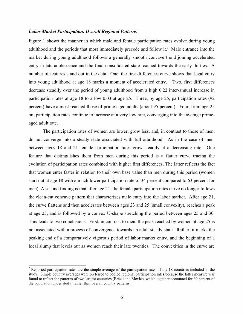
Labor Market Participation: Overall Regional Patterns Figure 1 shows the manner in which male and female participation rates evolve during young

adulthood and the periods that most immediately precede and follow it.2 Male entrance into the

market during young adulthood follows a generally smooth concave trend joining accelerated

entry in late adolescence and the final consolidated state reached towards the early thirties. A

number of features stand out in the data. One, the first differences curve shows that legal entry

into young adulthood at age 18 marks a moment of accelerated entry. Two, first differences

decrease steadily over the period of young adulthood from a high 0.22 inter-annual increase in

participation rates at age 18 to a low 0.03 at age 25. Three, by age 25, participation rates (92

percent) have almost reached those of prime-aged adults (about 95 percent). Four, from age 25

on, participation rates continue to increase at a very low rate, converging into the average prime-

aged adult rate.

The participation rates of women are lower, grow less, and, in contrast to those of men,

do not converge into a steady state associated with full adulthood. As in the case of men,

between ages 18 and 21 female participation rates grow steadily at a decreasing rate. One

feature that distinguishes them from men during this period is a flatter curve tracing the

evolution of participation rates combined with higher first differences. The latter reflects the fact

that women enter faster in relation to their own base value than men during this period (women

start out at age 18 with a much lower participation rate of 34 percent compared to 63 percent for

men). A second finding is that after age 21, the female participation rates curve no longer follows

the clean-cut concave pattern that characterizes male entry into the labor market. After age 21,

the curve flattens and then accelerates between ages 23 and 25 (small convexity), reaches a peak

at age 25, and is followed by a convex U-shape stretching the period between ages 25 and 30.

This leads to two conclusions. First, in contrast to men, the peak reached by women at age 25 is

not associated with a process of convergence towards an adult steady state. Rather, it marks the

peaking end of a comparatively vigorous period of labor market entry, and the beginning of a

local slump that levels out as women reach their late twenties. The convexities in the curve are

2 Reported participation rates are the simple average of the participation rates of the 18 countries included in the study. Simple country averages were preferred to pooled regional participation rates because the latter measure was found to reflect the patterns of two largest countries (Brazil and Mexico, which together accounted for 60 percent of the population under study) rather than overall country patterns.

6

very probably due to temporal entrances into full time child rearing,3 meaning that, in contrast to

men, participation in the labor market may be for many young adult females a provisional status.

Figure 1. Participation Rates in Latin America

Male participation rates in Latin America. Average of country rates.

-0.10

0.10.20.30.40.50.60.70.80.9

1

15 16 17 18 19 20 21 22 23 24 25 26 27 28 29 30 31 32 33 34 35

Particip. Rate First dif f . First dif f .(2yr.Mov.Av.)

Female participation rates in Latin America. Average of country rates.

-0.10

0.10.20.30.40.50.60.70.80.9

1

15 16 17 18 19 20 21 22 23 24 25 26 27 28 29 30 31 32 33 34 35

Particip. Rate First dif f . First dif f .(2yr.Mov.Av.)

Participation Rates of Young Adults by Education Level: Overall Regional Patterns Educational attainment determines when young adults enter the labor force. Figure 2 shows the

age-sequence of male and female participation rates in groups featuring different educational

attainments. A comparison of the curves in both graphs shows an overall pattern whereby

continued schooling implies postponement of entry into the labor market. But other than that,

patterns of men and women differ sharply. As seen in the figure, males enter young adulthood

(age 18) with a wide spread curves featuring higher participation rates among those with lower

levels of education; during young adulthood these curves follow a concave trajectory that

converges (by age 28) into a very narrow range (0.96-0.90) marking the standard participation

rates of all male adults. Convergence over young adulthood among males is as follows: at age

18, the range between the group featuring the highest participation rate and the group featuring

the lowest is 0.82-0.007; at age 21 the range 0.90-0.41, and at age 25, 0.95-0.82. Instead, female

curves start out with a lower spread between educational attainment groups at late adolescence

(0.33-0), their curves then merge into a knot of multiple crossings in the earlier part of young

adulthood (ages 18 to 23); by late young adulthood (age 25) their curves are more widely spread

(0.75-0.37) than in mid-adolescence, but in an inverse way, with groups with higher levels of

3 As shall be shown in the section that follows, the time at which such convexities occur varies by education level.

7

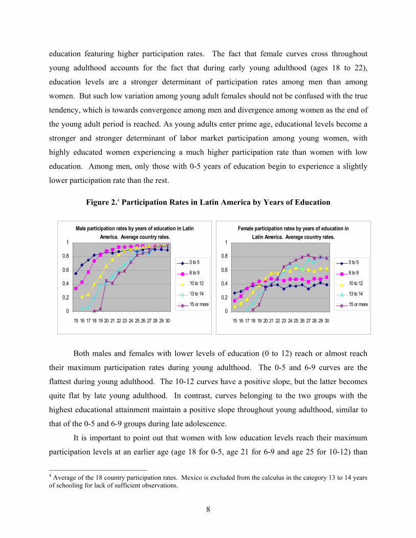
education featuring higher participation rates. The fact that female curves cross throughout

young adulthood accounts for the fact that during early young adulthood (ages 18 to 22),

education levels are a stronger determinant of participation rates among men than among

women. But such low variation among young adult females should not be confused with the true

tendency, which is towards convergence among men and divergence among women as the end of

the young adult period is reached. As young adults enter prime age, educational levels become a

stronger and stronger determinant of labor market participation among young women, with

highly educated women experiencing a much higher participation rate than women with low

education. Among men, only those with 0-5 years of education begin to experience a slightly

lower participation rate than the rest.

Figure 2.4 Participation Rates in Latin America by Years of Education

Male participation rates by years of education in Latin America. Average country rates.

0

0.2

0.4

0.6

0.8

1

15 16 17 18 19 20 21 22 23 24 25 26 27 28 29 30

0 to 5

6 to 9

10 to 12

13 to 14

15 or more

Female participation rates by years of education in Latin America. Average country rates.

0

0.2

0.4

0.6

0.8

1

15 16 17 18 19 20 21 22 23 24 25 26 27 28 29 30

0 to 5

6 to 9

10 to 12

13 to 14

15 or more

Both males and females with lower levels of education (0 to 12) reach or almost reach

their maximum participation rates during young adulthood. The 0-5 and 6-9 curves are the

flattest during young adulthood. The 10-12 curves have a positive slope, but the latter becomes

quite flat by late young adulthood. In contrast, curves belonging to the two groups with the

highest educational attainment maintain a positive slope throughout young adulthood, similar to

that of the 0-5 and 6-9 groups during late adolescence.

It is important to point out that women with low education levels reach their maximum

participation levels at an earlier age (age 18 for 0-5, age 21 for 6-9 and age 25 for 10-12) than

8

4 Average of the 18 country participation rates. Mexico is excluded from the calculus in the category 13 to 14 years of schooling for lack of sufficient observations.

their male equivalents, who at age 25 are still located in an increasing trend line with

participation rates that are still slightly lower than full adult participation. This means that men

with lower levels of education tend to continue entering the labor force as they move through

young adulthood, while females stop.

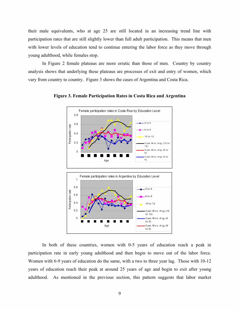
In Figure 2 female plateaus are more erratic than those of men. Country by country

analysis shows that underlying these plateaus are processes of exit and entry of women, which

vary from country to country. Figure 3 shows the cases of Argentina and Costa Rica.

Figure 3. Female Participation Rates in Costa Rica and Argentina

Female participation rates in Costa R ica by Education Level

0

0.2

0.4

0.6

0.8

Age

Parti

cipa

tion

rate

0 to 5

6 t o 9

1 0 t o 1 2

3 per. M ov. A vg . (1 0 t o1 2 )

3 per. M ov. A vg . (6 t o9 )

3 per. M ov. A vg . (0 t o5 )

Female participation rates in Argentina by Education Level

0

0.2

0.4

0.6

0.8

1

Age

Parti

cipa

tion

rate

0 to 5

6 to 9

10 to 12

3 per. M o v . A vg. (10to 12)

3 per. M o v . A vg. (0to 5)

3 per. M o v . A vg. (6to 9)

In both of these countries, women with 0-5 years of education reach a peak in

participation rate in early young adulthood and then begin to move out of the labor force.

Women with 6-9 years of education do the same, with a two to three year lag. Those with 10-12

years of education reach their peak at around 25 years of age and begin to exit after young

adulthood. As mentioned in the previous section, this pattern suggests that labor market

9

participation is a temporary state for many women, who then exit to enter full-time motherhood.

The pattern also suggests that as women opt for higher educational attainment they tend to

postpone childbearing decisions.

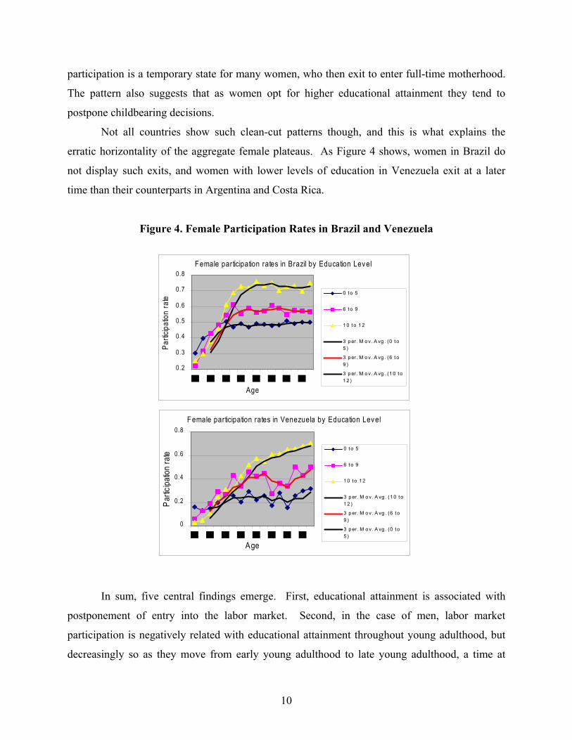
Not all countries show such clean-cut patterns though, and this is what explains the

erratic horizontality of the aggregate female plateaus. As Figure 4 shows, women in Brazil do

not display such exits, and women with lower levels of education in Venezuela exit at a later

time than their counterparts in Argentina and Costa Rica.

Figure 4. Female Participation Rates in Brazil and Venezuela

Female participation rates in Brazil by Education Level

0.2

0.3

0.4

0.5

0.6

0.7

0.8

Age

Parti

cipat

ion

rate

0 to 5

6 t o 9

1 0 t o 1 2

3 per. M ov. A vg . (0 t o5 )

3 per. M ov. A vg . (6 t o9 )

3 per. M ov. A vg . (1 0 t o1 2 )

Female participation rates in Venezuela by Education Level

0

0.2

0.4

0.6

0.8

Age

Partic

ipatio

n ra

te

0 t o 5

6 t o 9

10 t o 12

3 p er. M o v. A vg . (1 0 t o12 )

3 p er. M o v. A vg . (6 t o9 )

3 p er. M o v. A vg . (0 t o5 )

In sum, five central findings emerge. First, educational attainment is associated with

postponement of entry into the labor market. Second, in the case of men, labor market

participation is negatively related with educational attainment throughout young adulthood, but

decreasingly so as they move from early young adulthood to late young adulthood, a time at

10

which participation rates merge into a small range where variations by education level are almost

null. Third, in the case of women, in early young adulthood, educational attainment is not

clearly related with participation because during this period the curve representing different

educational attainments features multiple crossings. Differences emerge towards late young

adulthood when curves diverge in a pattern featuring high and ever increasing participation rates

among more educated women, and lower and stagnant participation rates among the less

educated. Fourth, participation rates of both males and females with 10 or more years of

education were found to grow continuously throughout young adulthood. Instead, those of

people with 9 or fewer years of education grew very slowly in the case of men; in the case of

women they stagnated and even diminished slightly after reaching a local peak in the early and

mid twenties. Finally, in some countries young adult women with nine or less years of education

experience decreases in participation after reaching local participation peaks during early young

adulthood. Sequential lags in this phenomenon by educational level suggest that as women opt

for higher educational attainment they tend to postpone childbearing decisions.

Country Differences in Young Adult Participation Figure 5 shows that there are important country differences in young adult participation. Among

men, such differences are much greater during early young adulthood (range: 0.55-0.84) than

during late young adulthood (range: 0.82-0.94), suggesting that convergence towards prime-age

adult participation rates, with greater postponement of entry in some countries that in others. As

expected from the previous section such convergence is not observed in the case of women.5

The most relevant country difference among the latter lies in the stair-type discontinuities

observed when the curve representing the participation rates of 23-25 year olds is ordered from

smallest to highest (see Figure 6). In order to explore these differences, the relationship between

participation rates and various country attributes were explored.

5 Range in early young adulthood>22-.53. Range in late young adulthood: 0.39-0.71.

11

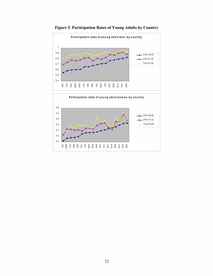
Figure 5. Participation Rates of Young Adults by Country

P a r ti c ip a tio n ra te s o f y o u n g a d u l t m e n , b y c o u n try

0.4

0.5

0.6

0.7

0.8

0.9

1

BOL

SLV

PAN

DOM

ARG

CO

L

VEN

PER

NIC

MEX CR

I

UR

Y

BRA

ECU

PRY

HON

P art 18-20

P art 21-22

P art 23-25

P a r ti c ip a tio n ra te s o f y o u n g a d u l t w o m e n , b y c o u n try

0.2

0.3

0.4

0.5

0.6

0.7

0.8

NIC

DOM

CHL

PAN

VEN

SLV

CR

I

MEX

HON

ARG

PRY

CO

L

BOL

GU

A

PER

ECU

UR

Y

BRA

P art 18-20

P art 21-22

P art 23-25

12

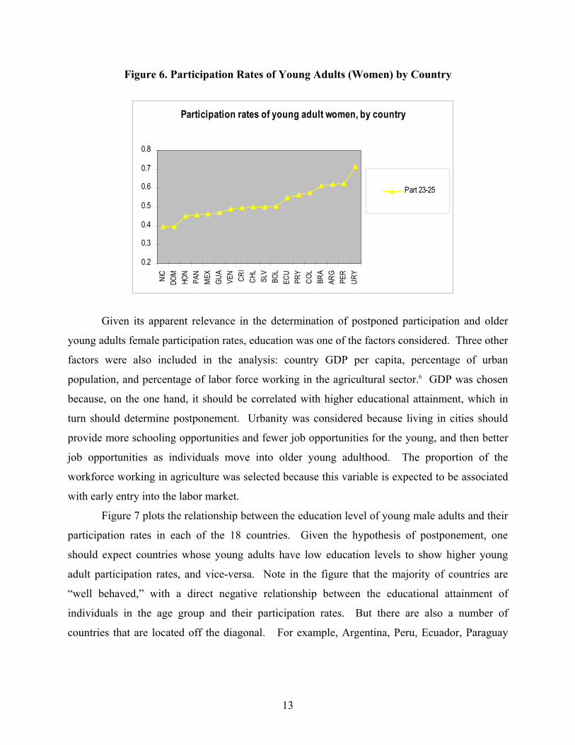
Figure 6. Participation Rates of Young Adults (Women) by Country

Participation rates of young adult women, by country

0.2

0.3

0.4

0.5

0.6

0.7

0.8NI

CDO

MHO

NPA

NM

EXGU

AVE

NCR

ICH

LSL

VBO

LEC

UPR

YCO

LBR

AAR

GPE

RUR

Y

Part 23-25

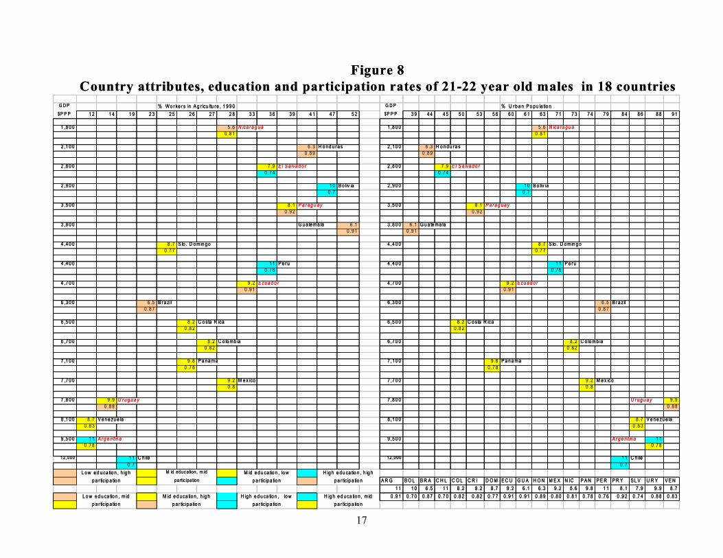
Given its apparent relevance in the determination of postponed participation and older

young adults female participation rates, education was one of the factors considered. Three other

factors were also included in the analysis: country GDP per capita, percentage of urban

population, and percentage of labor force working in the agricultural sector.6 GDP was chosen

because, on the one hand, it should be correlated with higher educational attainment, which in

turn should determine postponement. Urbanity was considered because living in cities should

provide more schooling opportunities and fewer job opportunities for the young, and then better

job opportunities as individuals move into older young adulthood. The proportion of the

workforce working in agriculture was selected because this variable is expected to be associated

with early entry into the labor market.

Figure 7 plots the relationship between the education level of young male adults and their

participation rates in each of the 18 countries. Given the hypothesis of postponement, one

should expect countries whose young adults have low education levels to show higher young

adult participation rates, and vice-versa. Note in the figure that the majority of countries are

“well behaved,” with a direct negative relationship between the educational attainment of

individuals in the age group and their participation rates. But there are also a number of

countries that are located off the diagonal. For example, Argentina, Peru, Ecuador, Paraguay

13

and Uruguay tend to combine high participation rates with high educational attainment, while

Nicaragua and El Salvador combine low participation rates with lower educational attainment.

The question was considered of whether young adults in the first group of countries were more

likely to combine school attendance with labor market participation, but no such relation was

found. The key difference seems to lie instead in educational attainment obtained by late

adolescence.

The possible impact of country GDP per capita, relative size of agricultural labor market

and relative size of urban population on the participation-schooling combination is explored in

Figure 7. The combination of low GDP and relatively large proportions of agricultural labor

and rural populations seems to “explain” the location of Honduras and Guatemala on the top-left

end of Figure 6, but not the location of Brazil, for the latter country has a comparatively high

GDP per capita and a rather small proportion of the labor force in the agricultural sector, and it is

largely urbanized. The two countries combining lower participation rates with low educational

level (Nicaragua and El Salvador) also feature very low GDP and high rurality. Such a

combination could be attributed to insufficient job opportunities in their post-war economies.

Figure 7 shows that there is little relation between country attributes and the location of

countries in the bottom right area of Figure 6. Chile is the only “well behaved” country,

combining low participation rates and high educational attainment (i.e., postponement of entry)

of mid-young adults with high GDP and high levels of urbanization. But then Bolivia and Peru,

two rather poor rural countries, also display low participation rates and high educational

attainment. It remains to be determined what accounts for this feature of Bolivia and Peru, but

aggressive educational policies may be at their root. Two other countries, which like Chile have

high GDP and low rurality, Argentina and Uruguay, feature comparatively high participation

rates relative to educational attainment. This characteristic of Argentina and Uruguay may be

accounted for by the large size of their population reaching retirement age relative to that of

young adults (see Figure 9), which combined with high GDP implies that a large number of older

people may be exiting large labor markets, leaving ample room for the young.

With the exception of Venezuela, all countries in the middle of the diagonal in Figure 6

are “well behaved” in Figure 7. That is, countries with middle levels of education and middle

6 All of these figures were obtained from the World Bank’s World Development Indicators (1998). GNP per capita is in dollars PPP.

14

level participation rates among young adult males, feature intermediate GDP, rurality and

agricultural labor force.

In sum, among males, participation rates tend to be negatively related to educational

attainment in all periods of young adulthood; participation-educational-attainment combinations

are in turn mildly related to country attributes such as GDP and rurality. Peru, Brazil and

Bolivia were the countries whose attributes most evidently did not relate as expected to

participation-educational-attainment combinations. Some countries were also found to be located

off the general diagonal of participation-educational-attainment combination. Hypotheses were

put out for four of countries located off the diagonal. The combination of high educational

attainment with relatively high participation rates in Argentina and Uruguay is possibly related to

the presence of a large elderly population that may be in the process of retirement. The

combination of low educational attainment and low participation in Nicaragua and El Salvador

may be related to the state of their economies.

15

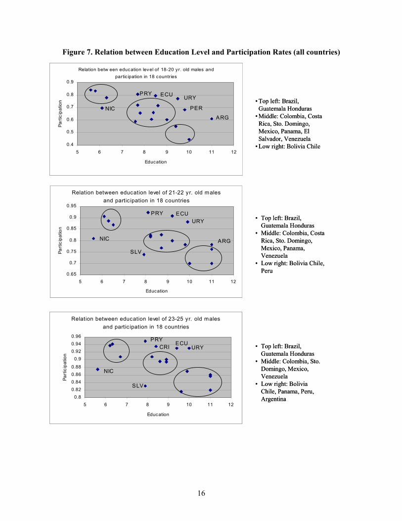
Figure 7. Relation between Education Level and Participation Rates (all countries)

• Top left: Brazil, Guatemala Honduras

• Middle: Colombia, Costa Rica, Sto. Domingo, Mexico, Panama, El Salvador, Venezuela

• Low right: Bolivia Chile


• Middle: Colombia, Costa Rica, Sto. Domingo, Mexico, Panama, Venezuela

• Low right: Bolivia Chile, Peru


• Middle: Colombia, Sto. Domingo, Mexico, Venezuela

• Low right: Bolivia Chile, Panama, Peru, Argentina

Relation betw een education level of 18-20 yr. old males and partic ipation in 18 countries

0.4

0.5

0.6

0.7

0.8

0.9

5 6 7 8 9 10 11 12

Education

Part

icip

atio

n

PRY ECU URY

ARG

PERNIC

Relation between education level of 21-22 yr. old males and partic ipation in 18 countries

0.65

0.7

0.75

0.8

0.85

0.9

0.95

5 6 7 8 9 10 11 12

Education

Part

icip

atio

n

NIC

SLV

PRY ECUURY

ARG


0.80.820.840.860.88

0.90.920.940.96

5 6 7 8 9 10 11 12

Education

Part

icip

atio

n

NIC

SLV

PRYECU

URYCRI


• Middle: Colombia, Costa Rica, Sto. Domingo, Mexico, Panama, El Salvador, Venezuela

• Low right: Bolivia Chile


• Middle: Colombia, Costa Rica, Sto. Domingo, Mexico, Panama, Venezuela

• Low right: Bolivia Chile, Peru


• Middle: Colombia, Sto. Domingo, Mexico, Venezuela

• Low right: Bolivia Chile, Panama, Peru, Argentina

Relation betw een education level of 18-20 yr. old males and partic ipation in 18 countries

0.4

0.5

0.6

0.7

0.8

0.9

5 6 7 8 9 10 11 12

Education

Part

icip

atio

n

PRY ECU URY

ARG

PERNIC


0.65

0.7

0.75

0.8

0.85

0.9

0.95

5 6 7 8 9 10 11 12

Education

Part

icip

atio

n

NIC

SLV

PRY ECUURY

ARG


0.80.820.840.860.88

0.90.920.940.96

5 6 7 8 9 10 11 12

Education

Part

icip

atio

n

NIC

SLV

PRYECU

URYCRI

16

% Wo r ke r s in A g r icu ltu r e , 1 9 9 0 % U r b a n P o p u la tio n1 2 1 4 1 9 2 3 2 5 2 6 2 7 2 8 3 3 3 6 3 9 4 1 4 7 5 2 3 9 4 4 4 5 5 0 5 3 5 6 6 0 6 1 6 3 7 1 7 3 7 4 7 9 8 4 8 6 8 8 9 1

1 ,8 0 0 5 .6 1 ,8 0 0 5 .6 0 .8 1 0 .8 1

2 ,1 0 0 6 .3 H o n d u r a s 2 ,1 0 0 6 .3 H o n d u r a s

0 .8 9 0 .8 9

2 ,8 0 0 7 .9 2 ,8 0 0 7 .9 0 .7 4 0 .7 4

2 ,9 0 0 1 0 B o liv ia 2 ,9 0 0 1 0 B o liv ia

0 .7 0 .7

3 ,5 0 0 8 .1 3 ,5 0 0 8 .1 0 .9 2 0 .9 2

3 ,8 0 0 G u a te ma la 6 .1 3 ,8 0 0 6 .1 G u a te ma la

0 .9 1 0 .9 1

4 ,4 0 0 8 .7 S to . D o min g o 4 ,4 0 0 8 .7 S to . D o min g o 0 .7 7 0 .7 7

4 ,4 0 0 1 1 P e r u 4 ,4 0 0 1 1 P e r u

0 .7 6 0 .7 6

4 ,7 0 0 9 .2 4 ,7 0 0 9 .2 0 .9 1 0 .9 1

6 ,3 0 0 6 .5 B r a zil 6 ,3 0 0 6 .5 B r a z il

0 .8 7 0 .8 7

6 ,5 0 0 8 .2 C o sta R ica 6 ,5 0 0 8 .2 C o sta R ica 0 .8 2 0 .8 2

6 ,7 0 0 8 .2 C o lo mb ia 6 ,7 0 0 8 .2 C o lo mb ia

0 .8 2 0 .8 2

7 ,1 0 0 9 .8 P a n a ma 7 ,1 0 0 9 .8 P a n a ma 0 .7 8 0 .7 8

7 ,7 0 0 9 .2 M e x ico 7 ,7 0 0 9 .2 M e x ico

0 .8 0 .8

7 ,8 0 0 9 .9 7 ,8 0 0 9 .90 .8 8 0 .8 8

8 ,1 0 0 8 .7 V e n e zu e la 8 ,1 0 0 8 .7 V e n e zu e la

0 .8 3 0 .8 3

9 ,5 0 0 1 1 9 ,5 0 0 1 10 .7 8 0 .7 8

12,000 1 1 C h ile 12,000 1 1 C h ile

0 .7 0 .7

A R G B O L B R A C H L C O L C R I D O M E C U G U A H O N M E X N IC P A N P E R P R Y S L V U R Y V E N1 1 1 0 6 .5 1 1 8 .2 8 .2 8 .7 9 .2 6 .1 6 .3 9 .2 5 .6 9 .8 1 1 8 .1 7 .9 9 .9 8 .7

0 .9 1 0 .7 0 0 .8 7 0 .7 0 0 .8 2 0 .8 2 0 .7 7 0 .9 1 0 .9 1 0 .8 9 0 .8 0 0 .8 1 0 .7 8 0 .7 6 0 .9 2 0 .7 4 0 .8 8 0 .8 3H ig h e d u ca tio n , lo w p a r tic ip a tio n

H ig h e d u ca tio n , m id p a r tic ip a tio n

M id e d u ca tio n , lo w p a r tic ip a tio n

L o w e d u ca tio n , m id p a r tic ip a tio n

M id e d u ca tio n , h ig h p a r tic ip a tio n

H ig h e d u ca tio n , h ig h p a r tic ip a tio n

G D P $P P P

G D P $P P P

L o w e d u ca tio n , h ig h p a r tic ip a tio n

M id educ ation, m id partic ipation

Figure 8Country attributes, education and participation rates of 21-22 year old males in 18 countries

% Wo r ke r s in A g r icu ltu r e , 1 9 9 0 % U r b a n P o p u la tio n1 2 1 4 1 9 2 3 2 5 2 6 2 7 2 8 3 3 3 6 3 9 4 1 4 7 5 2 3 9 4 4 4 5 5 0 5 3 5 6 6 0 6 1 6 3 7 1 7 3 7 4 7 9 8 4 8 6 8 8 9 1

1 ,8 0 0 5 .6 1 ,8 0 0 5 .6 0 .8 1 0 .8 1

2 ,1 0 0 6 .3 H o n d u r a s 2 ,1 0 0 6 .3 H o n d u r a s

0 .8 9 0 .8 9

2 ,8 0 0 7 .9 2 ,8 0 0 7 .9 0 .7 4 0 .7 4

2 ,9 0 0 1 0 B o liv ia 2 ,9 0 0 1 0 B o liv ia

0 .7 0 .7

3 ,5 0 0 8 .1 3 ,5 0 0 8 .1 0 .9 2 0 .9 2

3 ,8 0 0 G u a te ma la 6 .1 3 ,8 0 0 6 .1 G u a te ma la

0 .9 1 0 .9 1

4 ,4 0 0 8 .7 S to . D o min g o 4 ,4 0 0 8 .7 S to . D o min g o 0 .7 7 0 .7 7

4 ,4 0 0 1 1 P e r u 4 ,4 0 0 1 1 P e r u

0 .7 6 0 .7 6

4 ,7 0 0 9 .2 4 ,7 0 0 9 .2 0 .9 1 0 .9 1

6 ,3 0 0 6 .5 B r a zil 6 ,3 0 0 6 .5 B r a z il

0 .8 7 0 .8 7

6 ,5 0 0 8 .2 C o sta R ica 6 ,5 0 0 8 .2 C o sta R ica 0 .8 2 0 .8 2

6 ,7 0 0 8 .2 C o lo mb ia 6 ,7 0 0 8 .2 C o lo mb ia

0 .8 2 0 .8 2

7 ,1 0 0 9 .8 P a n a ma 7 ,1 0 0 9 .8 P a n a ma 0 .7 8 0 .7 8

7 ,7 0 0 9 .2 M e x ico 7 ,7 0 0 9 .2 M e x ico

0 .8 0 .8

7 ,8 0 0 9 .9 7 ,8 0 0 9 .90 .8 8 0 .8 8

8 ,1 0 0 8 .7 V e n e zu e la 8 ,1 0 0 8 .7 V e n e zu e la

0 .8 3 0 .8 3

9 ,5 0 0 1 1 9 ,5 0 0 1 10 .7 8 0 .7 8

12,000 1 1 C h ile 12,000 1 1 C h ile

0 .7 0 .7

A R G B O L B R A C H L C O L C R I D O M E C U G U A H O N M E X N IC P A N P E R P R Y S L V U R Y V E N1 1 1 0 6 .5 1 1 8 .2 8 .2 8 .7 9 .2 6 .1 6 .3 9 .2 5 .6 9 .8 1 1 8 .1 7 .9 9 .9 8 .7

0 .9 1 0 .7 0 0 .8 7 0 .7 0 0 .8 2 0 .8 2 0 .7 7 0 .9 1 0 .9 1 0 .8 9 0 .8 0 0 .8 1 0 .7 8 0 .7 6 0 .9 2 0 .7 4 0 .8 8 0 .8 3H ig h e d u ca tio n , lo w p a r tic ip a tio n

H ig h e d u ca tio n , m id p a r tic ip a tio n

M id e d u ca tio n , lo w p a r tic ip a tio n

L o w e d u ca tio n , m id p a r tic ip a tio n

M id e d u ca tio n , h ig h p a r tic ip a tio n

H ig h e d u ca tio n , h ig h p a r tic ip a tio n

G D P $P P P

G D P $P P P

L o w e d u ca tio n , h ig h p a r tic ip a tio n

M id educ ation, m id partic ipation

Figure 8Country attributes, education and participation rates of 21-22 year old males in 18 countries

N ica r a g u a N ica r a g u a

E l S a lva d o r E l S a lva d o r

P a r a g u a y P a r a g u a y

E cu a d o r E cu a d o r

U r u g u a y U r u g u a y

A r g e n tin a A r g e n tin a

N ica r a g u a N ica r a g u a

E l S a lva d o r E l S a lva d o r

P a r a g u a y P a r a g u a y

E cu a d o r E cu a d o r

U r u g u a y U r u g u a y

A r g e n tin a A r g e n tin a

17

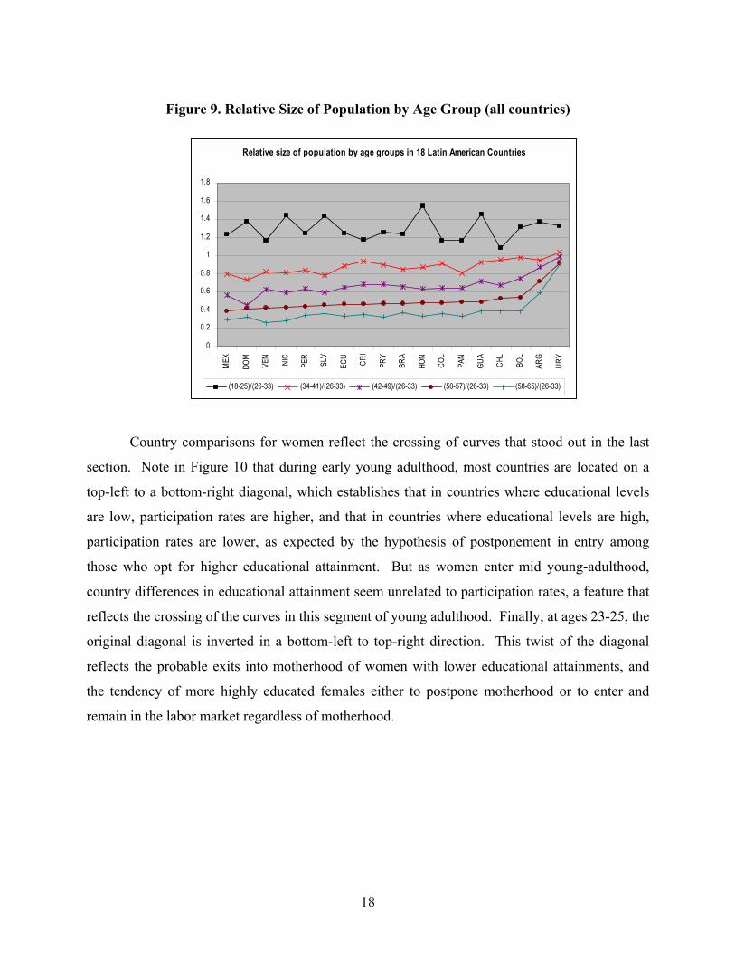
Figure 9. Relative Size of Population by Age Group (all countries)

Relative size of population by age groups in 18 Latin American Countries

0

0.2

0.4

0.6

0.8

1

1.2

1.4

1.6

1.8

MEX

DOM

VEN

NIC

PER

SLV

ECU

CRI

PRY

BRA

HON

COL

PAN

GUA

CHL

BOL

ARG

URY

(18-25)/(26-33) (34-41)/(26-33) (42-49)/(26-33) (50-57)/(26-33) (58-65)/(26-33)

Country comparisons for women reflect the crossing of curves that stood out in the last

section. Note in Figure 10 that during early young adulthood, most countries are located on a

top-left to a bottom-right diagonal, which establishes that in countries where educational levels

are low, participation rates are higher, and that in countries where educational levels are high,

participation rates are lower, as expected by the hypothesis of postponement in entry among

those who opt for higher educational attainment. But as women enter mid young-adulthood,

country differences in educational attainment seem unrelated to participation rates, a feature that

reflects the crossing of the curves in this segment of young adulthood. Finally, at ages 23-25, the

original diagonal is inverted in a bottom-left to top-right direction. This twist of the diagonal

reflects the probable exits into motherhood of women with lower educational attainments, and

the tendency of more highly educated females either to postpone motherhood or to enter and

remain in the labor market regardless of motherhood.

18

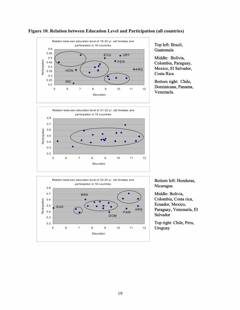
Figure 10. Relation between Education Level and Participation (all countries)

Relation betw een education level of 18-20 yr. old f emales and partic ipation in 18 countries

0.20.25

0.3

0.350.4

0.450.5

0.550.6

5 6 7 8 9 10 11 12

Education

Part

icip

atio

n

ECU URY

ARG

PER

NIC

HON


0.2

0.3

0.4

0.5

0.6

0.7

0.8

5 6 7 8 9 10 11 12

Education

Part

icip

atio

n


0.2

0.3

0.4

0.5

0.6

0.7

0.8

5 6 7 8 9 10 11 12

Education

Part

icip

atio

n

GUAARG

PANDOM

BRA

Bottom left: Honduras, Nicaragua

Middle: Bolivia, Colombia, Costa rica, Ecuador, Mexico, Paraguay, Venezuela, El Salvador

Top right: Chile, Peru, Uruguay

Top left: Brazil, Guatemala

Middle: Bolivia, Colombia, Paraguay, Mexico, El Salvador, Costa Rica

Bottom right: Chile, Dominicana, Panama, Venezuela.


0.20.25

0.3

0.350.4

0.450.5

0.550.6

5 6 7 8 9 10 11 12

Education

Part

icip

atio

n

ECU URY

ARG

PER

NIC

HON


0.2

0.3

0.4

0.5

0.6

0.7

0.8

5 6 7 8 9 10 11 12

Education

Part

icip

atio

n


0.2

0.3

0.4

0.5

0.6

0.7

0.8

5 6 7 8 9 10 11 12

Education

Part

icip

atio

n

GUAARG

PANDOM

BRA

Bottom left: Honduras, Nicaragua

Middle: Bolivia, Colombia, Costa rica, Ecuador, Mexico, Paraguay, Venezuela, El Salvador

Top right: Chile, Peru, Uruguay

Top left: Brazil, Guatemala

Middle: Bolivia, Colombia, Paraguay, Mexico, El Salvador, Costa Rica

Bottom right: Chile, Dominicana, Panama, Venezuela.

19

W o m e n a g e s 1 8 to 2 0 W o m e n a g e s 2 3 to 2 5% W o rk e rs in A g r ic u l tu re , 1 9 9 0 % W o rk e rs in A g r ic u l tu re , 1 9 9 0

$ P P P 1 2 1 4 1 9 2 3 2 5 2 6 2 7 2 8 3 3 3 6 3 9 4 1 4 7 5 2 $ P P P 1 2 1 4 1 9 2 3 2 5 2 6 2 7 2 8 3 3 3 6 3 9 4 1 4 7 5 2

1 ,8 0 0 6 .4 9 N ica ra g u a 1 ,8 0 0 7 .0 N ica ra g u a 0 .2 1 8 0 .3 9 5

2 ,1 0 0 6 .6 7 H o n d u r a s 2 ,1 0 0 6 .7 6 9 H o n d u ra s

0 .3 6 9 0 .4 5

2 ,8 0 0 7 .7 2 7 E l S a lv a d o r 2 ,8 0 0 7 .6 6 E l S a lv a d o r 0 .3 3 9 0 .4 9 9

2 ,9 0 0 B o liv ia 8 .5 3 8 2 ,9 0 0 B o liv ia 8 .8 7 1

0 .4 3 3 0 .5 0 5

3 ,5 0 0 8 .1 6 5 P a r a g u a y 3 ,5 0 0 8 .1 8 1 P a r a g u a y 0 .4 0 .5 6 5

3 ,8 0 0 G u a te ma la 5 .3 3 9 3 ,8 0 0 G u a te ma la 5 .0 3 6

0 .4 5 5 0 .4 7

4 ,4 0 0 9 .2 6 4 S to . D o min g o 4 ,4 0 0 9 .3 S to . D o min g o 0 .2 6 4 0 .3 9 7

4 ,4 0 0 9 .7 4 5 P e r u 4 ,4 0 0 1 0 .3 7 P e ru

0 .4 6 8 0 .6 2 4

4 ,7 0 0 8 .9 3 E cu a d o r 4 ,7 0 0 9 .2 7 4 E cu a d o r 0 .5 0 .5 4 9

6 ,3 0 0 7 .0 3 B r a zil 6 ,3 0 0 7 .4 8 2 B r a zil

0 .5 3 4 0 .6 1 3

6 ,5 0 0 8 .3 9 7 C ta . R ica 6 ,5 0 0 8 .3 4 6 C ta . R ica 0 .3 6 3 0 .4 9 6

6 ,7 0 0 8 .4 5 C o lo mb ia 6 ,7 0 0 8 .5 8 7 C o lo mb ia

0 .4 1 2 0 .5 7 5

7 ,1 0 0 9 .8 0 9 P a n a ma 7 ,1 0 0 1 0 .6 3 P a n a ma 0 .2 7 9 0 .4 5 9

7 ,7 0 0 8 .4 1 2 M e x ico 7 ,7 0 0 8 .8 3 7 M e x ico

0 .3 6 6 0 .4 6 3

7 ,8 0 0 1 0 .1 3 U r u g u a y 7 ,8 0 0 1 0 .8 1 U r u g u a y 0 .5 2 9 0 .7 1 4

8 ,1 0 0 9 .1 7 5 V e n e zu e la 8 ,1 0 0 9 .4 5 V e n e zu e la

0 .2 9 5 0 .4 8 7

9 ,5 0 0 1 1 .1 9 A rg e n tin a 9 ,5 0 0 1 1 .5 1 A r g e n tin a 0 .3 7 6 0 .6 2 1

1 2 ,0 0 0 1 0 .6 2 C h ile 1 2 ,0 0 0 1 1 .5 1 C h ile

0 .2 7 7 0 .4 9 9 H ig h e d u ca tio n , lo w

p a r ticip a tio n

M id e d u ca tio n , h ig h p a r ticip a tio n

L o w e d u ca tio n , mid p a r ticip a tio n

H ig h e d u ca tio n , h ig h p a r ticip a tio n

H ig h e d u ca tio n , mid p a r ticip a tio n

M id e d u ca tio n , mid p a r ticip a tio n

L o w e d u ca tio n , h ig h p a r ticip a tio n

L o w e d u ca tio n , lo w p a r ticip a tio n

M id e d u ca tio n , lo w p a r ticip a tio n

Figure 11

Country attributes, education and participation rates of 18-20 and 23-25 year old females in 18 countriesW o m e n a g e s 1 8 to 2 0 W o m e n a g e s 2 3 to 2 5

% W o rk e rs in A g r ic u l tu re , 1 9 9 0 % W o rk e rs in A g r ic u l tu re , 1 9 9 0$ P P P 1 2 1 4 1 9 2 3 2 5 2 6 2 7 2 8 3 3 3 6 3 9 4 1 4 7 5 2 $ P P P 1 2 1 4 1 9 2 3 2 5 2 6 2 7 2 8 3 3 3 6 3 9 4 1 4 7 5 2

1 ,8 0 0 6 .4 9 N ica ra g u a 1 ,8 0 0 7 .0 N ica ra g u a 0 .2 1 8 0 .3 9 5

2 ,1 0 0 6 .6 7 H o n d u r a s 2 ,1 0 0 6 .7 6 9 H o n d u ra s

0 .3 6 9 0 .4 5

2 ,8 0 0 7 .7 2 7 E l S a lv a d o r 2 ,8 0 0 7 .6 6 E l S a lv a d o r 0 .3 3 9 0 .4 9 9

2 ,9 0 0 B o liv ia 8 .5 3 8 2 ,9 0 0 B o liv ia 8 .8 7 1

0 .4 3 3 0 .5 0 5

3 ,5 0 0 8 .1 6 5 P a r a g u a y 3 ,5 0 0 8 .1 8 1 P a r a g u a y 0 .4 0 .5 6 5

3 ,8 0 0 G u a te ma la 5 .3 3 9 3 ,8 0 0 G u a te ma la 5 .0 3 6

0 .4 5 5 0 .4 7

4 ,4 0 0 9 .2 6 4 S to . D o min g o 4 ,4 0 0 9 .3 S to . D o min g o 0 .2 6 4 0 .3 9 7

4 ,4 0 0 9 .7 4 5 P e r u 4 ,4 0 0 1 0 .3 7 P e ru

0 .4 6 8 0 .6 2 4

4 ,7 0 0 8 .9 3 E cu a d o r 4 ,7 0 0 9 .2 7 4 E cu a d o r 0 .5 0 .5 4 9

6 ,3 0 0 7 .0 3 B r a zil 6 ,3 0 0 7 .4 8 2 B r a zil

0 .5 3 4 0 .6 1 3

6 ,5 0 0 8 .3 9 7 C ta . R ica 6 ,5 0 0 8 .3 4 6 C ta . R ica 0 .3 6 3 0 .4 9 6

6 ,7 0 0 8 .4 5 C o lo mb ia 6 ,7 0 0 8 .5 8 7 C o lo mb ia

0 .4 1 2 0 .5 7 5

7 ,1 0 0 9 .8 0 9 P a n a ma 7 ,1 0 0 1 0 .6 3 P a n a ma 0 .2 7 9 0 .4 5 9

7 ,7 0 0 8 .4 1 2 M e x ico 7 ,7 0 0 8 .8 3 7 M e x ico

0 .3 6 6 0 .4 6 3

7 ,8 0 0 1 0 .1 3 U r u g u a y 7 ,8 0 0 1 0 .8 1 U r u g u a y 0 .5 2 9 0 .7 1 4

8 ,1 0 0 9 .1 7 5 V e n e zu e la 8 ,1 0 0 9 .4 5 V e n e zu e la

0 .2 9 5 0 .4 8 7

9 ,5 0 0 1 1 .1 9 A rg e n tin a 9 ,5 0 0 1 1 .5 1 A r g e n tin a 0 .3 7 6 0 .6 2 1

1 2 ,0 0 0 1 0 .6 2 C h ile 1 2 ,0 0 0 1 1 .5 1 C h ile

0 .2 7 7 0 .4 9 9 H ig h e d u ca tio n , lo w

p a r ticip a tio n

M id e d u ca tio n , h ig h p a r ticip a tio n

L o w e d u ca tio n , mid p a r ticip a tio n

H ig h e d u ca tio n , h ig h p a r ticip a tio n

H ig h e d u ca tio n , mid p a r ticip a tio n

M id e d u ca tio n , mid p a r ticip a tio n

L o w e d u ca tio n , h ig h p a r ticip a tio n

L o w e d u ca tio n , lo w p a r ticip a tio n

M id e d u ca tio n , lo w p a r ticip a tio n

Figure 11

Country attributes, education and participation rates of 18-20 and 23-25 year old females in 18 countries

20

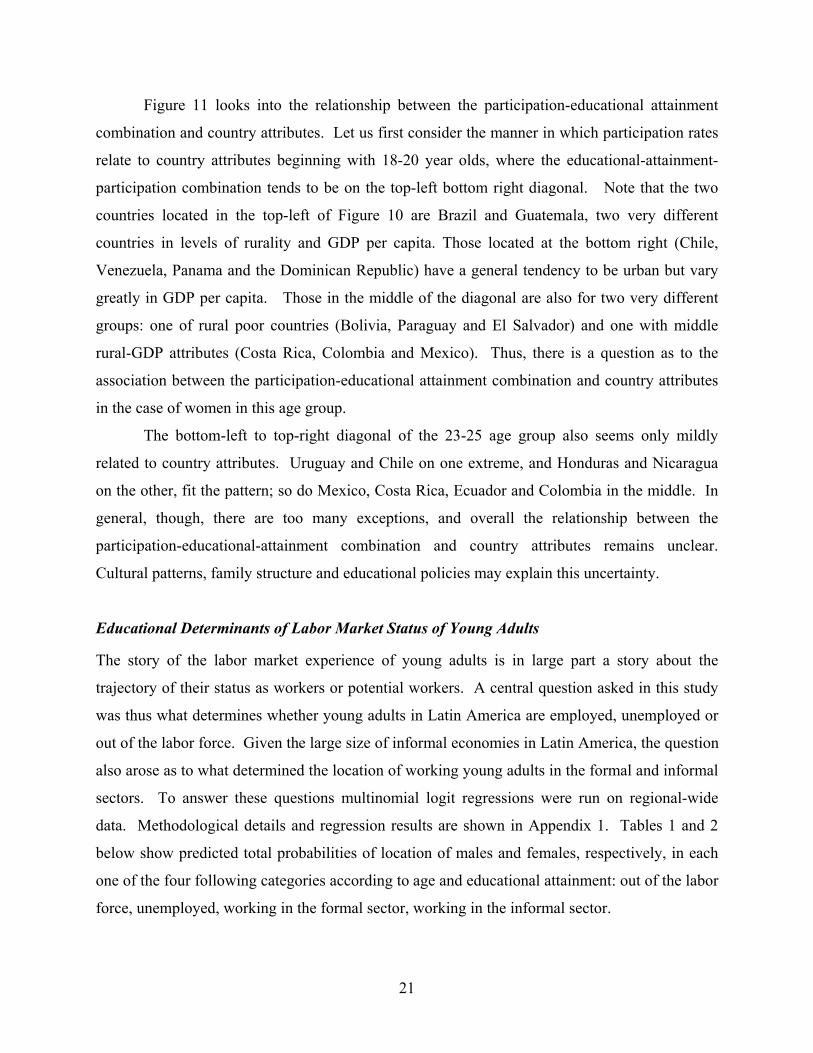
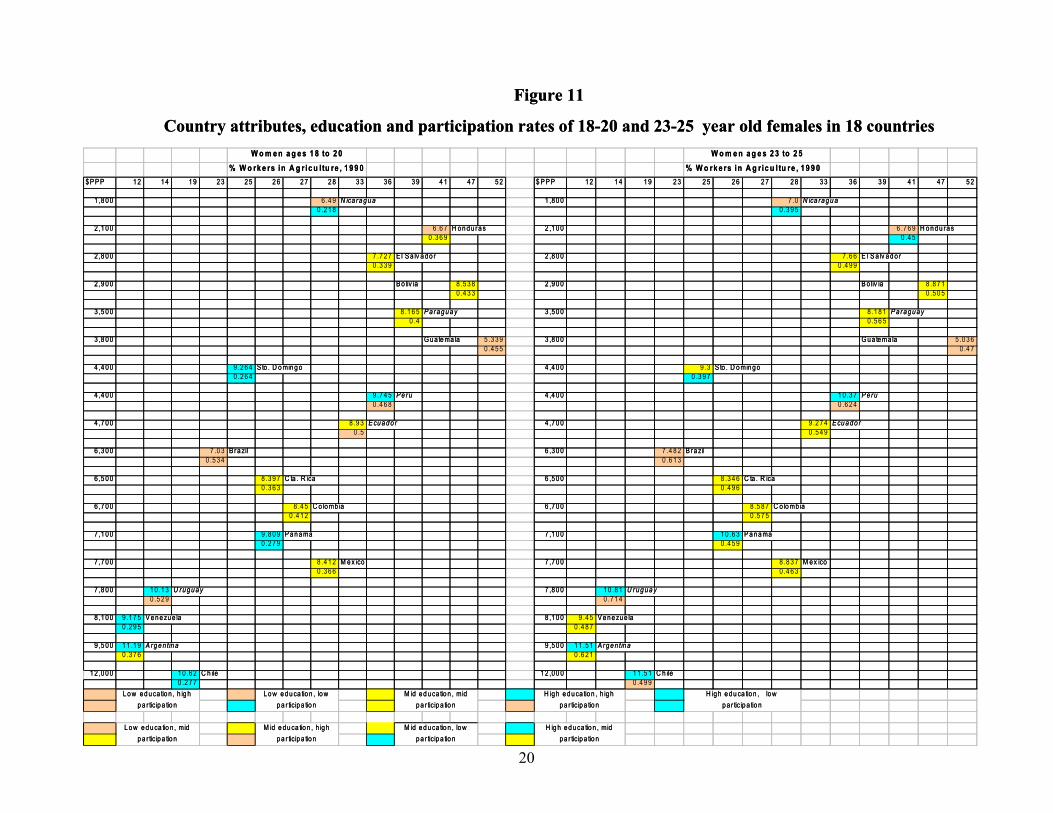
Figure 11 looks into the relationship between the participation-educational attainment

combination and country attributes. Let us first consider the manner in which participation rates

relate to country attributes beginning with 18-20 year olds, where the educational-attainment-

participation combination tends to be on the top-left bottom right diagonal. Note that the two

countries located in the top-left of Figure 10 are Brazil and Guatemala, two very different

countries in levels of rurality and GDP per capita. Those located at the bottom right (Chile,

Venezuela, Panama and the Dominican Republic) have a general tendency to be urban but vary

greatly in GDP per capita. Those in the middle of the diagonal are also for two very different

groups: one of rural poor countries (Bolivia, Paraguay and El Salvador) and one with middle

rural-GDP attributes (Costa Rica, Colombia and Mexico). Thus, there is a question as to the

association between the participation-educational attainment combination and country attributes

in the case of women in this age group.

The bottom-left to top-right diagonal of the 23-25 age group also seems only mildly

related to country attributes. Uruguay and Chile on one extreme, and Honduras and Nicaragua

on the other, fit the pattern; so do Mexico, Costa Rica, Ecuador and Colombia in the middle. In

general, though, there are too many exceptions, and overall the relationship between the

participation-educational-attainment combination and country attributes remains unclear.

Cultural patterns, family structure and educational policies may explain this uncertainty.

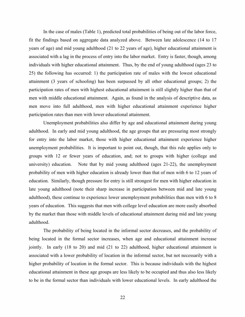
Educational Determinants of Labor Market Status of Young Adults The story of the labor market experience of young adults is in large part a story about the

trajectory of their status as workers or potential workers. A central question asked in this study

was thus what determines whether young adults in Latin America are employed, unemployed or

out of the labor force. Given the large size of informal economies in Latin America, the question

also arose as to what determined the location of working young adults in the formal and informal

sectors. To answer these questions multinomial logit regressions were run on regional-wide

data. Methodological details and regression results are shown in Appendix 1. Tables 1 and 2

below show predicted total probabilities of location of males and females, respectively, in each

one of the four following categories according to age and educational attainment: out of the labor

force, unemployed, working in the formal sector, working in the informal sector.

21

In the case of males (Table 1), predicted total probabilities of being out of the labor force,

fit the findings based on aggregate data analyzed above. Between late adolescence (14 to 17

years of age) and mid young adulthood (21 to 22 years of age), higher educational attainment is

associated with a lag in the process of entry into the labor market. Entry is faster, though, among

individuals with higher educational attainment. Thus, by the end of young adulthood (ages 23 to

25) the following has occurred: 1) the participation rate of males with the lowest educational

attainment (3 years of schooling) has been surpassed by all other educational groups; 2) the

participation rates of men with highest educational attainment is still slightly higher than that of

men with middle educational attainment. Again, as found in the analysis of descriptive data, as

men move into full adulthood, men with higher educational attainment experience higher

participation rates than men with lower educational attainment.

Unemployment probabilities also differ by age and educational attainment during young

adulthood. In early and mid young adulthood, the age groups that are pressuring most strongly

for entry into the labor market, those with higher educational attainment experience higher

unemployment probabilities. It is important to point out, though, that this rule applies only to

groups with 12 or fewer years of education, and; not to groups with higher (college and

university) education. Note that by mid young adulthood (ages 21-22), the unemployment

probability of men with higher education is already lower than that of men with 6 to 12 years of

education. Similarly, though pressure for entry is still strongest for men with higher education in

late young adulthood (note their sharp increase in participation between mid and late young

adulthood), these continue to experience lower unemployment probabilities than men with 6 to 8

years of education. This suggests that men with college level education are more easily absorbed

by the market than those with middle levels of educational attainment during mid and late young

adulthood.

The probability of being located in the informal sector decreases, and the probability of

being located in the formal sector increases, when age and educational attainment increase

jointly. In early (18 to 20) and mid (21 to 22) adulthood, higher educational attainment is

associated with a lower probability of location in the informal sector, but not necessarily with a

higher probability of location in the formal sector. This is because individuals with the highest

educational attainment in these age groups are less likely to be occupied and thus also less likely

to be in the formal sector than individuals with lower educational levels. In early adulthood the

22

probability of being located in the formal sector is within the 22 percent to 28 percent range in all

educational (3, 6, 9 and 12 years of education) groups. As men in each of these educational

groups move into mid-young adulthood, their probability of being located in the formal sector

increases more in higher educational groups than in lower educational groups. By late

adulthood, men with upper secondary education have a 52.76 percent probability of being

located in the formal sector, while tje probability among men with three years of education has

risen only from 22 percent to 25.32 percent between early and late adulthood. As with the case

of unemployment probability, men with higher (college) education never experience a low

probability of being located in the formal sector. In mid adulthood (21-22), when they begin to

enter the labor market, their probability of being located in the formal sector (40.61 percent) is

already almost as high as that of men with upper secondary education (45.25 percent). In late

young adulthood, when they massively enter the labor market, their probability of being located

in the formal sector (about 65 percent) is far above that of men with 12 years of education (52.76

percent). Again, this suggests that the formal sectors of Latin American economies most easily

absorb college and university graduates.

The probability of being located in the informal sector generally7 rises slightly with age,

regardless of educational attainment, even for men with college or university education. While

the possibility of a modeling problem cannot be discarded, such small continuous increases may

be picking up the tendency of men to set up their own small businesses as they move into prime

age.8

Though overestimating the probability of being in the labor force for women with

educational attainment below higher education, estimations of the probability of female location

outside of the labor force generally fit the patterns found through descriptive statistics. In early

young adulthood, women are much more likely than their male age-education equivalents to be

out of the labor force. At that age, moreover, females with upper secondary education are more

likely to be out of the labor force than women with 6 or fewer years of education. As women

move into late young adulthood, those with higher educational levels experience rapid entry into

the labor force. Instead, women with a lower educational level reach a low local peak in labor

market participation in mid-adulthood. They then proceed to move back out of the labor force

7 A small slump is observed in the movement from late adulthood into the early thirties. 8 Recall that informality is operationalized as working in a company with 5 or fewer workers.

23

throughout late young adulthood in the case of women with 3 years of education, and with a lag,

through the early thirties among women with 6 years of education (the childbearing slump).9

A cross-over in female participation rates occurs in late young adulthood (23 to 25 years

of age) according to the model (at age 21 in descriptive statistics). As women move into their

early thirties, the probability of being out of the labor force falls sharply to 22 percent among

those with higher education (similar to descriptive statistics), while it remains about the same (47

percent) among those with lower educational levels.

The Probability of unemployment is lowest among women with high and low educational

attainment, and highest among women with middle educational attainment. The apparently high

capacity of formal economies to absorb individuals with college education may explain the low

unemployment probability of women with high educational attainment. The low unemployment

probability among women with low educational levels may instead result from their higher

tendency to stay out of the labor force, and their tendency to seek and find work in the more

flexible informal sector of the economy. Assuming the above processes are true, the higher

probability of unemployment of women with middle levels of education may derive from the

stronger pressure they put on entry into the market and the formal sector in particular, combined

with the lower capacity of the latter sector to absorb them.

The patterns in Table 2 provide some support to the above hypotheses. First, note that

the unemployment probability of women with 3 years of education is high during early

adulthood (18-20), just when these are pushing into the market. Unemployment probability

decreases sharply when they reach ages 21 to 22, when the inter-period movement into the labor

force also sharply decreases. Note that women with higher educational attainment not only show

higher unemployment probabilities at this age (21-22), but also experienced a much smaller

reduction in relation to the previous period. It is then the stronger push of these more educated

women between ages 18-20 and 21-22 into the labor force that explains the persistence of high

unemployment rates in mid young adulthood. Second, note that the highest unemployment

probability of college graduates taking place in late young adulthood (moment at which they

massively seen entrance into the market) is lower than that which had been experienced by

women of other educational levels at the time in which they were entering the market. The fact

that educated women’s probabilities of unemployment are relatively low regardless of their

9 Note that the model fails to predict the slump for women with 9 and 12 years of education.

24

strong push into the formal sector at that age (23-25) suggests that the formal sector is highly

capable of absorbing them.

As in the case of men, the location of women in the formal sector increases with the joint

growth of education and age. The inverse, though, is not consistently true in the case of the

informal sector, especially in the middle levels of education. This may be due to women’s lower

ability to enter the formal sector at mid levels of education, and their subsequent opting for the

informal sector. It is important to note that throughout young adulthood, the proportion of

occupied women with 6 to 9 years of education in the informal sector is consistently higher than

that of men, and that as women age, this feature tends to accentuate.

25

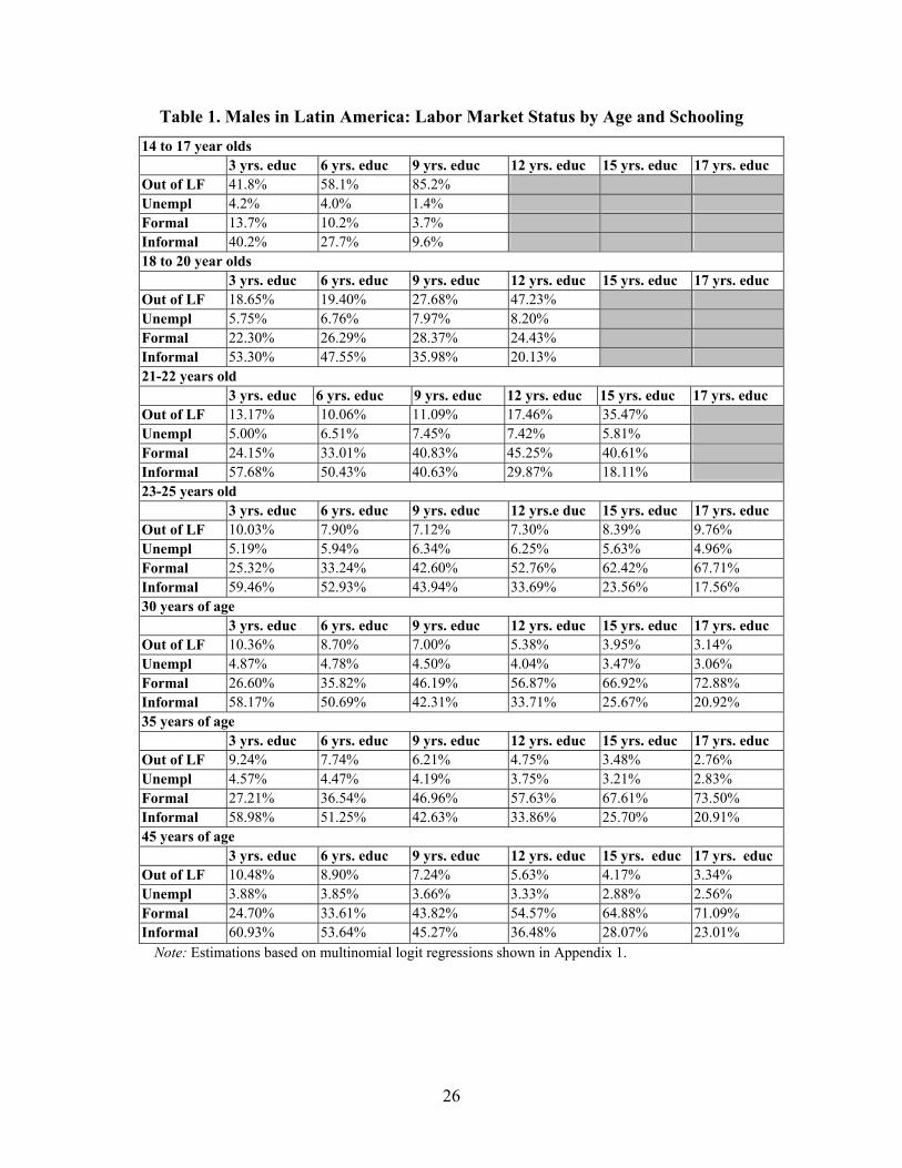
Table 1. Males in Latin America: Labor Market Status by Age and Schooling 14 to 17 year olds 3 yrs. educ 6 yrs. educ 9 yrs. educ 12 yrs. educ 15 yrs. educ 17 yrs. educ Out of LF 41.8% 58.1% 85.2% Unempl 4.2% 4.0% 1.4% Formal 13.7% 10.2% 3.7% Informal 40.2% 27.7% 9.6% 18 to 20 year olds 3 yrs. educ 6 yrs. educ 9 yrs. educ 12 yrs. educ 15 yrs. educ 17 yrs. educ Out of LF 18.65% 19.40% 27.68% 47.23% Unempl 5.75% 6.76% 7.97% 8.20% Formal 22.30% 26.29% 28.37% 24.43% Informal 53.30% 47.55% 35.98% 20.13% 21-22 years old 3 yrs. educ 6 yrs. educ 9 yrs. educ 12 yrs. educ 15 yrs. educ 17 yrs. educ Out of LF 13.17% 10.06% 11.09% 17.46% 35.47% Unempl 5.00% 6.51% 7.45% 7.42% 5.81% Formal 24.15% 33.01% 40.83% 45.25% 40.61% Informal 57.68% 50.43% 40.63% 29.87% 18.11% 23-25 years old 3 yrs. educ 6 yrs. educ 9 yrs. educ 12 yrs.e duc 15 yrs. educ 17 yrs. educ Out of LF 10.03% 7.90% 7.12% 7.30% 8.39% 9.76% Unempl 5.19% 5.94% 6.34% 6.25% 5.63% 4.96% Formal 25.32% 33.24% 42.60% 52.76% 62.42% 67.71% Informal 59.46% 52.93% 43.94% 33.69% 23.56% 17.56% 30 years of age 3 yrs. educ 6 yrs. educ 9 yrs. educ 12 yrs. educ 15 yrs. educ 17 yrs. educ Out of LF 10.36% 8.70% 7.00% 5.38% 3.95% 3.14% Unempl 4.87% 4.78% 4.50% 4.04% 3.47% 3.06% Formal 26.60% 35.82% 46.19% 56.87% 66.92% 72.88% Informal 58.17% 50.69% 42.31% 33.71% 25.67% 20.92% 35 years of age 3 yrs. educ 6 yrs. educ 9 yrs. educ 12 yrs. educ 15 yrs. educ 17 yrs. educ Out of LF 9.24% 7.74% 6.21% 4.75% 3.48% 2.76% Unempl 4.57% 4.47% 4.19% 3.75% 3.21% 2.83% Formal 27.21% 36.54% 46.96% 57.63% 67.61% 73.50% Informal 58.98% 51.25% 42.63% 33.86% 25.70% 20.91% 45 years of age 3 yrs. educ 6 yrs. educ 9 yrs. educ 12 yrs. educ 15 yrs. educ 17 yrs. educ Out of LF 10.48% 8.90% 7.24% 5.63% 4.17% 3.34% Unempl 3.88% 3.85% 3.66% 3.33% 2.88% 2.56% Formal 24.70% 33.61% 43.82% 54.57% 64.88% 71.09% Informal 60.93% 53.64% 45.27% 36.48% 28.07% 23.01%

Note: Estimations based on multinomial logit regressions shown in Appendix 1.

26

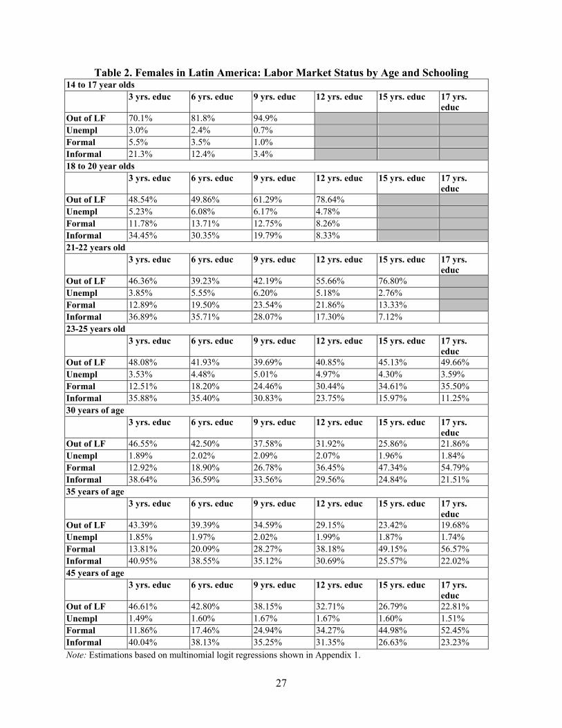
Table 2. Females in Latin America: Labor Market Status by Age and Schooling 14 to 17 year olds 3 yrs. educ 6 yrs. educ 9 yrs. educ 12 yrs. educ 15 yrs. educ 17 yrs.

educ Out of LF 70.1% 81.8% 94.9% Unempl 3.0% 2.4% 0.7% Formal 5.5% 3.5% 1.0% Informal 21.3% 12.4% 3.4% 18 to 20 year olds 3 yrs. educ 6 yrs. educ 9 yrs. educ 12 yrs. educ 15 yrs. educ 17 yrs.

educ Out of LF 48.54% 49.86% 61.29% 78.64% Unempl 5.23% 6.08% 6.17% 4.78% Formal 11.78% 13.71% 12.75% 8.26% Informal 34.45% 30.35% 19.79% 8.33% 21-22 years old 3 yrs. educ 6 yrs. educ 9 yrs. educ 12 yrs. educ 15 yrs. educ 17 yrs.

educ Out of LF 46.36% 39.23% 42.19% 55.66% 76.80% Unempl 3.85% 5.55% 6.20% 5.18% 2.76% Formal 12.89% 19.50% 23.54% 21.86% 13.33% Informal 36.89% 35.71% 28.07% 17.30% 7.12% 23-25 years old 3 yrs. educ 6 yrs. educ 9 yrs. educ 12 yrs. educ 15 yrs. educ 17 yrs.

educ Out of LF 48.08% 41.93% 39.69% 40.85% 45.13% 49.66% Unempl 3.53% 4.48% 5.01% 4.97% 4.30% 3.59% Formal 12.51% 18.20% 24.46% 30.44% 34.61% 35.50% Informal 35.88% 35.40% 30.83% 23.75% 15.97% 11.25% 30 years of age 3 yrs. educ 6 yrs. educ 9 yrs. educ 12 yrs. educ 15 yrs. educ 17 yrs.



educ Out of LF 46.61% 42.80% 38.15% 32.71% 26.79% 22.81% Unempl 1.49% 1.60% 1.67% 1.67% 1.60% 1.51% Formal 11.86% 17.46% 24.94% 34.27% 44.98% 52.45% Informal 40.04% 38.13% 35.25% 31.35% 26.63% 23.23% Note: Estimations based on multinomial logit regressions shown in Appendix 1.

27

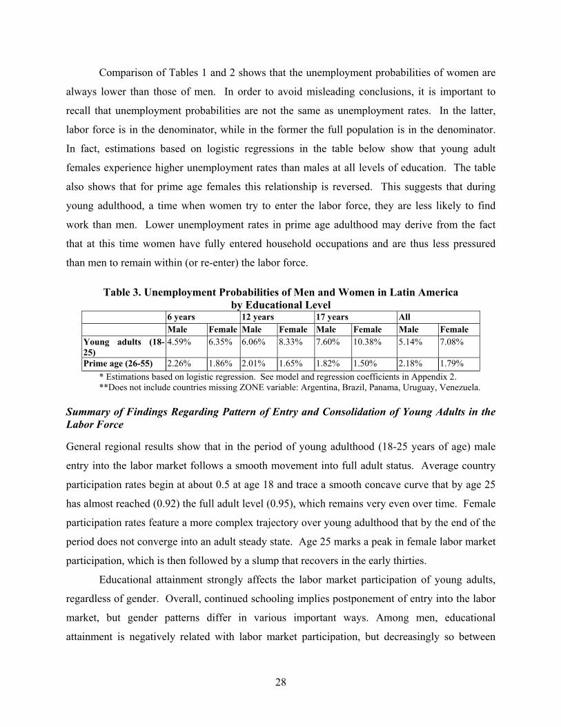
Comparison of Tables 1 and 2 shows that the unemployment probabilities of women are

always lower than those of men. In order to avoid misleading conclusions, it is important to

recall that unemployment probabilities are not the same as unemployment rates. In the latter,

labor force is in the denominator, while in the former the full population is in the denominator.

In fact, estimations based on logistic regressions in the table below show that young adult

females experience higher unemployment rates than males at all levels of education. The table

also shows that for prime age females this relationship is reversed. This suggests that during

young adulthood, a time when women try to enter the labor force, they are less likely to find

work than men. Lower unemployment rates in prime age adulthood may derive from the fact

that at this time women have fully entered household occupations and are thus less pressured

than men to remain within (or re-enter) the labor force. Table 3. Unemployment Probabilities of Men and Women in Latin America

by Educational Level 6 years 12 years 17 years All Male Female Male Female Male Female Male Female Young adults (18-25)

4.59% 6.35% 6.06% 8.33% 7.60% 10.38% 5.14% 7.08%

Prime age (26-55) 2.26% 1.86% 2.01% 1.65% 1.82% 1.50% 2.18% 1.79% * Estimations based on logistic regression. See model and regression coefficients in Appendix 2. **Does not include countries missing ZONE variable: Argentina, Brazil, Panama, Uruguay, Venezuela.

Summary of Findings Regarding Pattern of Entry and Consolidation of Young Adults in the Labor Force General regional results show that in the period of young adulthood (18-25 years of age) male

entry into the labor market follows a smooth movement into full adult status. Average country

participation rates begin at about 0.5 at age 18 and trace a smooth concave curve that by age 25

has almost reached (0.92) the full adult level (0.95), which remains very even over time. Female

participation rates feature a more complex trajectory over young adulthood that by the end of the

period does not converge into an adult steady state. Age 25 marks a peak in female labor market

participation, which is then followed by a slump that recovers in the early thirties.

Educational attainment strongly affects the labor market participation of young adults,

regardless of gender. Overall, continued schooling implies postponement of entry into the labor

market, but gender patterns differ in various important ways. Among men, educational

attainment is negatively related with labor market participation, but decreasingly so between

28

early and late young adulthood. Instead, among women, educational attainment is not clearly

related with participation because at this time the curves representing participation of groups

with different levels of educational attainment feature multiple crossings. Differences among

women emerge towards late young adulthood, a time at which the more educated begin to

experience high and increasing participation rates, while the less educated feature low and

stagnant participation rates.

Country by country analysis of female participation by educational attainment showed

that in many, though not all countries (Brazil being an important exception), the curves tracing

participation by educational attainment reach a peak, followed by evident decreases in

participation that are very possibly due to entry into motherhood. As education levels increase,

these peaks occur at a later age, meaning that among women motherhood is postponed as

educational attainment increases. The pattern also supports the proposition that for many

women, labor market participation is a temporary state that precedes full time motherhood.

In general, in countries where young male adults have higher levels of education, young

adult male participation rates are lower, but a number of countries did not fit this pattern.

Argentina and Uruguay show a combination of high educational attainment with high

participation rates. Nicaragua and El Salvador show a combination of low educational

attainment and low participation rates. Country attributes such as GDP and rurality were found

to be only mildly associated with participation-educational-attainment combinations observed in

the different countries. Other factors such as education policies and the relative size of various

age groups may be behind some of the unexplained differences.

The association between educational attainment and participation rates varied over

different moments of young adulthood in country comparison analysis. In early young

adulthood, females in countries with higher educational attainment generally display lower

participation rates. But during mid young adulthood, no such relation is evident, and by late

young adulthood this relation is reversed. This coincides with the finding that better educated

women experience higher levels of labor market participation. As in the case of men, country

attributes such as GDP and rurality were found to be only mildly associated with the

participation-educational-attainment combinations of women observed in the different countries.

Status analysis shows that, among young adults, the probability of being located in the

formal sector of the economy rises with educational attainment. It was also found that among

29

women the probability of being out of the labor force decreases with educational attainment.

Finally, the probability of being in a state of unemployment is higher among higher educated

younger young adults, but lower among older young adults.

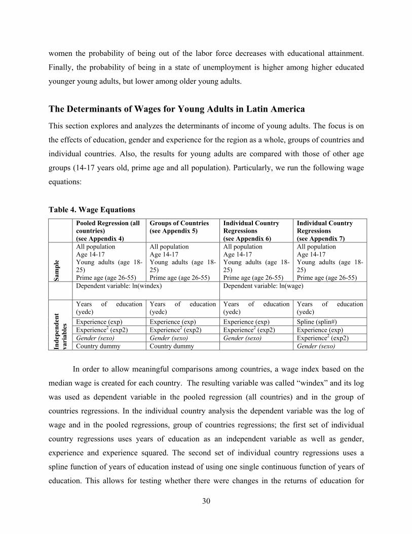
The Determinants of Wages for Young Adults in Latin America This section explores and analyzes the determinants of income of young adults. The focus is on

the effects of education, gender and experience for the region as a whole, groups of countries and

individual countries. Also, the results for young adults are compared with those of other age

groups (14-17 years old, prime age and all population). Particularly, we run the following wage

equations:

Table 4. Wage Equations Pooled Regression (all

countries) (see Appendix 4)

Groups of Countries (see Appendix 5)

Individual Country Regressions (see Appendix 6)

Individual Country Regressions (see Appendix 7)

Sam

ple

All population Age 14-17 Young adults (age 18-25) Prime age (age 26-55)




Dependent variable: ln(windex) Dependent variable: ln(wage)

Years of education (yedc)




Experience (exp) Experience (exp) Experience (exp) Spline (splin#) Experience2 (exp2) Experience2 (exp2) Experience2 (exp2) Experience (exp) Gender (sexo) Gender (sexo) Gender (sexo) Experience2 (exp2)

Inde

pend

ent

vari

able

s

Country dummy Country dummy Gender (sexo)

In order to allow meaningful comparisons among countries, a wage index based on the

median wage is created for each country. The resulting variable was called “windex” and its log

was used as dependent variable in the pooled regression (all countries) and in the group of

countries regressions. In the individual country analysis the dependent variable was the log of

wage and in the pooled regressions, group of countries regressions; the first set of individual

country regressions uses years of education as an independent variable as well as gender,

experience and experience squared. The second set of individual country regressions uses a

spline function of years of education instead of using one single continuous function of years of

education. This allows for testing whether there were changes in the returns of education for

30

threshold values of years of education. The rest of the variables were the same as those used in

the other regressions (in the pooled regressions and group of countries regressions country

dummies were also used to take into account country-specific effects). Finally, earning

differentials were also estimated for each country by educational level using the linear regression

analysis suggested by Freeman (1979). The earning differentials for educational level by country

make it possible to analyze with more detail the effect of education among age groups and

educational levels by country and groups of countries.

Effect of Education on Earnings The regression’s results for the region as a whole (see Appendix 4) show positive and significant

returns for education for young adults in Latin America. The level of returns for young adults

(13.6 percent) is similar to those obtained for late adolescents (13.1 percent) and prime age

adults (13.4 percent). These results suggest that workers realize most of the benefits of education

immediately after entering the labor market.

Freeman’s regressions for males make it possible to explore with more detail the earning

differentials for education by country, age group and educational level. The age-earning profile

constructed using the results of the Freeman’s regression including all countries (see Table 5 and

Figure 12) shows that earning increases continuously with age and educational level. During the

period of young adulthood there is a sharp marginal change in the return for education compared

to late adolescence (14 to 17 years of age). The returns keep increasing during this period of life

although the marginal changes in the returns for education are larger for prime age adults of 26

to 45 years old than the marginal changes occurring during young adulthood.

31

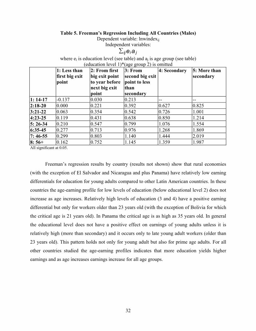
Table 5. Freeman’s Regression Including All Countries (Males) Dependent variable: lnwindexij

Independent variables: ∑ij ji ae

where ei is education level (see table) and aj is age group (see table) (education level 1)*(age group 2) is omitted

1: Less than first big exit point

2: From first big exit point to year before next big exit point

3: From second big exit point to less than secondary

4: Secondary 5: More than secondary

1: 14-17 -0.137 0.030 0.213 -- -- 2:18-20 0.000 0.221 0.392 0.627 0.825 3:21-22 0.063 0.354 0.542 0.726 1.001 4:23-25 0.119 0.431 0.638 0.850 1.214 5: 26-34 0.210 0.547 0.799 1.076 1.554 6:35-45 0.277 0.713 0.976 1.268 1.869 7: 46-55 0.299 0.803 1.140 1.444 2.019 8: 56+ 0.162 0.752 1.145 1.359 1.987 All significant at 0.05.

Freeman’s regression results by country (results not shown) show that rural economies

(with the exception of El Salvador and Nicaragua and plus Panama) have relatively low earning

differentials for education for young adults compared to other Latin American countries. In these

countries the age-earning profile for low levels of education (below educational level 2) does not

increase as age increases. Relatively high levels of education (3 and 4) have a positive earning

differential but only for workers older than 23 years old (with the exception of Bolivia for which

the critical age is 21 years old). In Panama the critical age is as high as 35 years old. In general

the educational level does not have a positive effect on earnings of young adults unless it is

relatively high (more than secondary) and it occurs only to late young adult workers (older than

23 years old). This pattern holds not only for young adult but also for prime age adults. For all

other countries studied the age-earning profiles indicates that more education yields higher

earnings and as age increases earnings increase for all age groups.

32

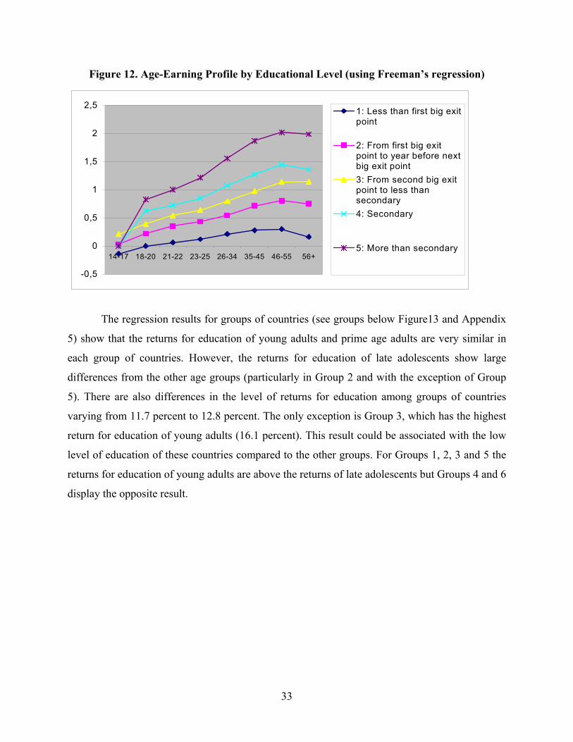
Figure 12. Age-Earning Profile by Educational Level (using Freeman’s regression)

-0,5

0

0,5

1

1,5

2

2,5

14-17 18-20 21-22 23-25 26-34 35-45 46-55 56+

1: Less than first big exitpoint

2: From first big exitpoint to year before nextbig exit point3: From second big exitpoint to less thansecondary4: Secondary

5: More than secondary

The regression results for groups of countries (see groups below Figure13 and Appendix

5) show that the returns for education of young adults and prime age adults are very similar in

each group of countries. However, the returns for education of late adolescents show large

differences from the other age groups (particularly in Group 2 and with the exception of Group

5). There are also differences in the level of returns for education among groups of countries

varying from 11.7 percent to 12.8 percent. The only exception is Group 3, which has the highest

return for education of young adults (16.1 percent). This result could be associated with the low

level of education of these countries compared to the other groups. For Groups 1, 2, 3 and 5 the

returns for education of young adults are above the returns of late adolescents but Groups 4 and 6

display the opposite result.

33

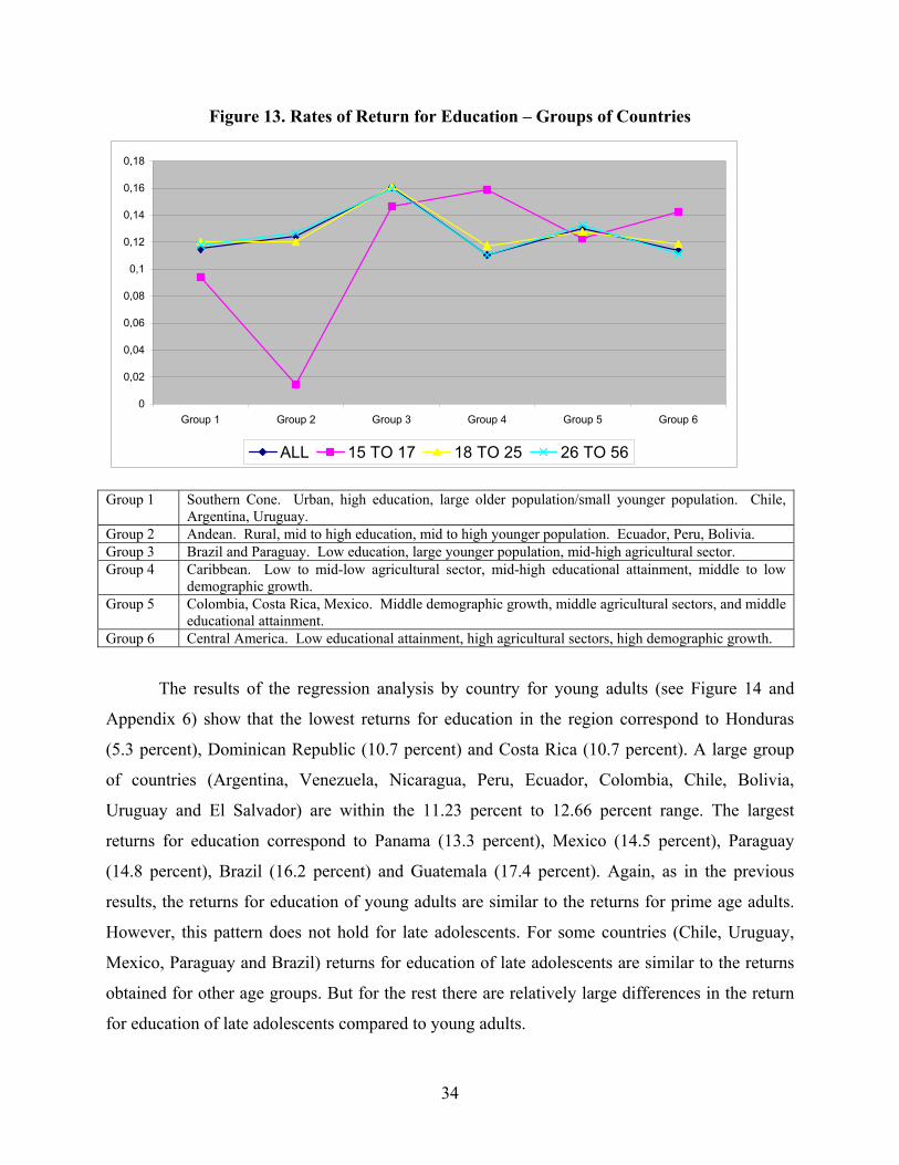
Figure 13. Rates of Return for Education – Groups of Countries

0

0,02

0,04

0,06

0,08

0,1

0,12

0,14

0,16

0,18

Group 1 Group 2 Group 3 Group 4 Group 5 Group 6

ALL 15 TO 17 18 TO 25 26 TO 56

Group 1 Southern Cone. Urban, high education, large older population/small younger population. Chile,

Argentina, Uruguay. Group 2 Andean. Rural, mid to high education, mid to high younger population. Ecuador, Peru, Bolivia. Group 3 Brazil and Paraguay. Low education, large younger population, mid-high agricultural sector. Group 4 Caribbean. Low to mid-low agricultural sector, mid-high educational attainment, middle to low

demographic growth. Group 5 Colombia, Costa Rica, Mexico. Middle demographic growth, middle agricultural sectors, and middle

educational attainment. Group 6 Central America. Low educational attainment, high agricultural sectors, high demographic growth.

The results of the regression analysis by country for young adults (see Figure 14 and

Appendix 6) show that the lowest returns for education in the region correspond to Honduras

(5.3 percent), Dominican Republic (10.7 percent) and Costa Rica (10.7 percent). A large group

of countries (Argentina, Venezuela, Nicaragua, Peru, Ecuador, Colombia, Chile, Bolivia,

Uruguay and El Salvador) are within the 11.23 percent to 12.66 percent range. The largest

returns for education correspond to Panama (13.3 percent), Mexico (14.5 percent), Paraguay

(14.8 percent), Brazil (16.2 percent) and Guatemala (17.4 percent). Again, as in the previous

results, the returns for education of young adults are similar to the returns for prime age adults.

However, this pattern does not hold for late adolescents. For some countries (Chile, Uruguay,

Mexico, Paraguay and Brazil) returns for education of late adolescents are similar to the returns

obtained for other age groups. But for the rest there are relatively large differences in the return

for education of late adolescents compared to young adults.

34

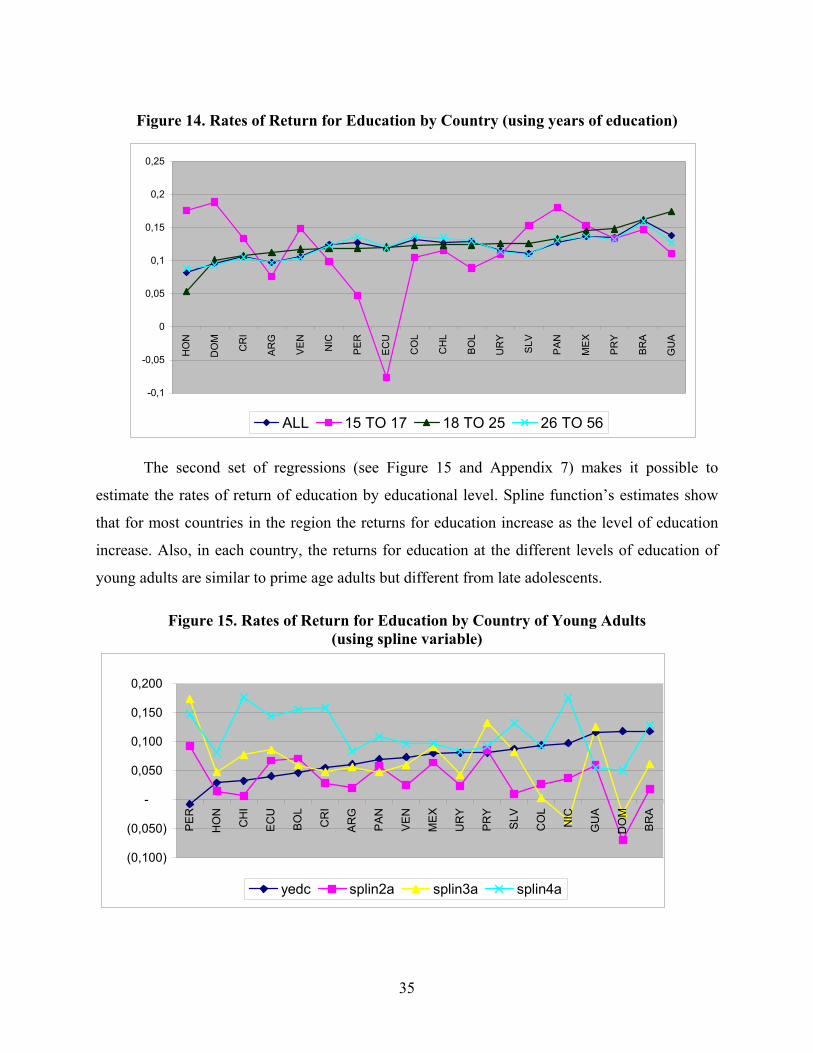
Figure 14. Rates of Return for Education by Country (using years of education)

-0,1

-0,05

0

0,05

0,1

0,15

0,2

0,25

HO

N

DO

M

CR

I

ARG

VEN

NIC

PER

ECU

CO

L

CH

L

BOL

UR

Y

SLV

PAN

MEX

PRY

BRA

GU

A

ALL 15 TO 17 18 TO 25 26 TO 56

The second set of regressions (see Figure 15 and Appendix 7) makes it possible to

estimate the rates of return of education by educational level. Spline function’s estimates show

that for most countries in the region the returns for education increase as the level of education

increase. Also, in each country, the returns for education at the different levels of education of

young adults are similar to prime age adults but different from late adolescents.

Figure 15. Rates of Return for Education by Country of Young Adults (using spline variable)

(0,100)

(0,050)

-

0,050

0,100

0,150

0,200

PER

HO

N

CH

I

ECU

BOL

CR

I

ARG

PAN

VEN

MEX

UR

Y

PRY

SLV

CO

L

NIC

GU

A

DO

M

BRA

yedc splin2a splin3a splin4a

35

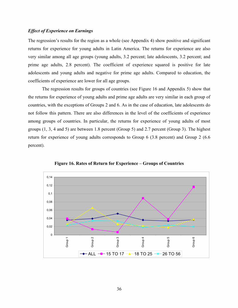
Effect of Experience on Earnings The regression’s results for the region as a whole (see Appendix 4) show positive and significant

returns for experience for young adults in Latin America. The returns for experience are also

very similar among all age groups (young adults, 3.2 percent; late adolescents, 3.2 percent; and

prime age adults, 2.8 percent). The coefficient of experience squared is positive for late

adolescents and young adults and negative for prime age adults. Compared to education, the

coefficients of experience are lower for all age groups.

The regression results for groups of countries (see Figure 16 and Appendix 5) show that

the returns for experience of young adults and prime age adults are very similar in each group of

countries, with the exceptions of Groups 2 and 6. As in the case of education, late adolescents do

not follow this pattern. There are also differences in the level of the coefficients of experience

among groups of countries. In particular, the returns for experience of young adults of most

groups (1, 3, 4 and 5) are between 1.8 percent (Group 5) and 2.7 percent (Group 3). The highest

return for experience of young adults corresponds to Group 6 (3.8 percent) and Group 2 (6.6

percent).

Figure 16. Rates of Return for Experience – Groups of Countries

0

0,02

0,04

0,06

0,08

0,1

0,12

0,14

Gro

up 1

Gro

up 2

Gro

up 3

Gro

up 4

Gro

up 5

Gro

up 6

ALL 15 TO 17 18 TO 25 26 TO 56

36

The regression results by country (see Figure 17 and Appendix 6) show that the returns

for experience of young adults are negative for Paraguay, Chile and Colombia. Even though the

other countries exhibit positive values for experience there are large differences among

countries, varying from 0.2 percent to 10 percent. Compared to late adolescents, prime age adults

tend to have returns for experience closer to those of young adults.

Figure 17. Rates of Return for Experience by Country (using years of education)

-0,1

-0,05

0

0,05

0,1

0,15

0,2

0,25

0,3

PRY

CH

L

CO

L

CR

I

HO

N

NIC

VEN

BOL

PAN

BRA

DO

M

ARG

GU

A

SLV

MEX

UR

Y

PER

ECU

ALL 15 TO 17 18 TO 25 26 TO 56

The spline function results show a change in the level of the experience coefficient of

young adults compared to the results obtained in the first set of individual country regressions

(using only years of education as proxy of education). Although the relative order of countries is

similar, but not identical, the coefficients of experience are systematically higher. This pattern

also holds for the results of experience for prime age adults but not for late adolescents. Returns

for experience of young adults show large variation among countries, ranging from 2.1 percent in

Colombia to 14.4 percent in Ecuador.

Another interesting feature is that returns for experience of young adults are consistently

higher than those obtained for prime age adults in almost all countries (the exception are Bolivia

and Colombia). The smallest differences in returns for experience between young adults and

prime age adults occur in the countries with the lowest return for experience for young adults

(Colombia, Honduras, Chile and Bolivia), while the countries in the middle range are Nicaragua,

37

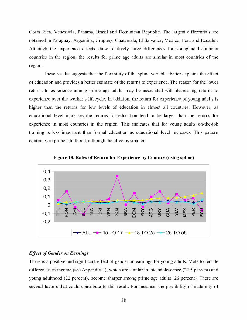
Costa Rica, Venezuela, Panama, Brazil and Dominican Republic. The largest differentials are

obtained in Paraguay, Argentina, Uruguay, Guatemala, El Salvador, Mexico, Peru and Ecuador.

Although the experience effects show relatively large differences for young adults among

countries in the region, the results for prime age adults are similar in most countries of the

region.

These results suggests that the flexibility of the spline variables better explains the effect

of education and provides a better estimate of the returns to experience. The reason for the lower

returns to experience among prime age adults may be associated with decreasing returns to

experience over the worker’s lifecycle. In addition, the return for experience of young adults is

higher than the returns for low levels of education in almost all countries. However, as

educational level increases the returns for education tend to be larger than the returns for

experience in most countries in the region. This indicates that for young adults on-the-job

training is less important than formal education as educational level increases. This pattern

continues in prime adulthood, although the effect is smaller.

Figure 18. Rates of Return for Experience by Country (using spline)

-0,2

-0,1

0

0,1

0,2

0,3

0,4

CO

L

HO

N

CH

I

BOL

NIC

CR

I

VEN

PAN

BRA

DO

M

PRY

ARG

UR

Y

GU

A

SLV

MEX

PER

ECU

ALL 15 TO 17 18 TO 25 26 TO 56

Effect of Gender on Earnings

There is a positive and significant effect of gender on earnings for young adults. Male to female

differences in income (see Appendix 4), which are similar in late adolescence (22.5 percent) and

young adulthood (22 percent), become sharper among prime age adults (26 percent). There are

several factors that could contribute to this result. For instance, the possibility of maternity of

38

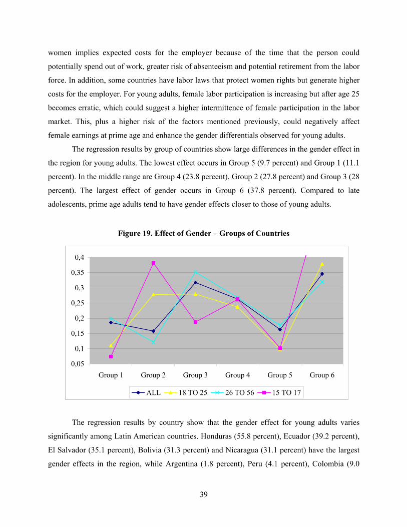
women implies expected costs for the employer because of the time that the person could

potentially spend out of work, greater risk of absenteeism and potential retirement from the labor

force. In addition, some countries have labor laws that protect women rights but generate higher

costs for the employer. For young adults, female labor participation is increasing but after age 25

becomes erratic, which could suggest a higher intermittence of female participation in the labor

market. This, plus a higher risk of the factors mentioned previously, could negatively affect

female earnings at prime age and enhance the gender differentials observed for young adults.

The regression results by group of countries show large differences in the gender effect in

the region for young adults. The lowest effect occurs in Group 5 (9.7 percent) and Group 1 (11.1

percent). In the middle range are Group 4 (23.8 percent), Group 2 (27.8 percent) and Group 3 (28

percent). The largest effect of gender occurs in Group 6 (37.8 percent). Compared to late

adolescents, prime age adults tend to have gender effects closer to those of young adults.

Figure 19. Effect of Gender – Groups of Countries

0,05

0,1

0,15

0,2

0,25

0,3

0,35

0,4

Group 1 Group 2 Group 3 Group 4 Group 5 Group 6

ALL 18 TO 25 26 TO 56 15 TO 17

The regression results by country show that the gender effect for young adults varies

significantly among Latin American countries. Honduras (55.8 percent), Ecuador (39.2 percent),

El Salvador (35.1 percent), Bolivia (31.3 percent) and Nicaragua (31.1 percent) have the largest

gender effects in the region, while Argentina (1.8 percent), Peru (4.1 percent), Colombia (9.0

39

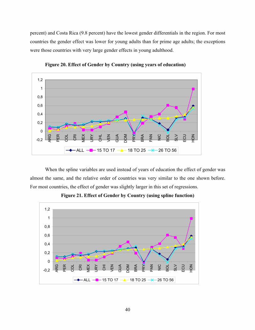
percent) and Costa Rica (9.8 percent) have the lowest gender differentials in the region. For most

countries the gender effect was lower for young adults than for prime age adults; the exceptions

were those countries with very large gender effects in young adulthood.

Figure 20. Effect of Gender by Country (using years of education)

-0,2

0

0,2

0,4

0,6

0,8

1

1,2

ARG

PER

CO

L

CR

I

MEX

UR

Y

CH

L

VEN

GU

A

DO

M

PRY

BRA

PAN

NIC

BOL

SLV

ECU

HO

N

ALL 15 TO 17 18 TO 25 26 TO 56

When the spline variables are used instead of years of education the effect of gender was

almost the same, and the relative order of countries was very similar to the one shown before.

For most countries, the effect of gender was slightly larger in this set of regressions.

Figure 21. Effect of Gender by Country (using spline function)

-0,2

0

0,2

0,4

0,6

0,8

1

1,2

ARG

PER

CO

L

CR

I

MEX

UR

Y

CH

I

VEN

GU

A

DO

M

BRA

PRY

PAN

NIC

BOL

SLV

ECU

HO

N

ALL 15 TO 17 18 TO 25 26 TO 56

40

References Becker, G. 1991. A Treatise on the Family. Enlarged edition. Cambridge, United States: Harvard

University Press.

Becker, G., and N. Tomes. 1993. “Human Capital and the Rise and Fall of Families.” In: G.

Becker, editor. Human Capital. Third edition. Chicago, United States: University of

Chicago Press

Behrman, J., and P. Taubman. 1995. “Birth Order, Schooling, and Earnings.” In: J. Behrman, R.

Pollack and P. Taubman, editors. From Parent to Child. Intrahousehold Allocations and

Intergenerational Relations in the United States. Chicago, United States: University of

Chicago Press.

Behrman, J., and B. Wolfe 1984. “The Socioeconomic Impact of Schooling in a Developing

Country.” Review of Economics and Statistics 66: 296-303.

Cartaya, V.F. 1989. La pobreza y la economía informal: ¿Casualidad o causalidad? Simposios-

IESA. Caracas: Ediciones IESA.

Ellwood, D.T. 1989. “Teenage Unemployment: Permanent Scars or Temporary Blemishes?” In:

R.B. Freeman and D.A. Wise, editors. The Youth Labor Market Problem: Its Nature,

Causes and Consequences. Chicago, United States: University of Chicago Press.

Feldstein, M. 1973. “The Economics of the New Unemployment.” Public Interest (33): 3-42.

Freeman, R.B. 1979. “The Effects of Demographic Factors on Age-Earnings Profiles.” Journal

of Human Resources 14(3): 289-313.

Freeman, R.B., and D.A. Wise. 1982. “The Youth Labor Market Problem: Its Nature, Causes,

and Consequences.” In: R.B. Freeman and D.A. Wise, editors. The Youth Labor Market

Problem: Its Nature, Causes, and Consequences. Chicago, United States: University of

Chicago Press.

Fuller, R., and S.F. Seninger. 1984. “A Discriminant Analysis of Factors Affecting the

Employment of Urban Youth.” Applied Economics 16.

Gabriel, P.E., D.R. Williams and S. Schmitz. 1990. “The Relative Occupational Attainment of

Young Blacks, Whites and Hispanics.” Southern Economic Journal 57(2): 35-46.

Hamilton, S.F. 1990. Apprenticeship for Adulthood. New York, United States: Free Press.

Heckman, J., and J. Hotz. 1986. “An Investigation of the Labor Market Earnings of Panamanian

Males: Evaluating the Sources of Inequality.” Journal of Human Resources 21: 507-42.

41

Juhn, C., K. Murphy and B. Pierce. 1993. “Wage Inequality and the Rise in Returns to Skill.”

Journal of Political Economy 101(3): 410-42.

Kiefer, N.M. 1988. “Economic Duration Data and Hazard Functions.” Journal of Economic

Literature 26(2): 646-79.

Korenman, S., and D. Neumark. 1997. “Cohort Crowding and Youth Labor Market: A Cross-

National Analysis.” NBER Working Paper 6031. Cambridge, United States: National

Bureau of Economic Research.

Lam, D., and R. Schoeni. 1993. “Effects of Family Background on Earnings and Returns to

Schooling: Evidence from Brazil.” Journal of Political Economy 101(4): 710-40.

Macunovich, D.J. 1998. “Relative Cohort Size and Inequality in the United States.” American

Economic Review 88(2): 259-64.

Mazumdar, D. 1976. “The Urban Informal Sector.” World Development 4(8): 655-79.

Miller, P.W. 1989. “Low-Wage Youth Employment: A Permanent or Transitory State?”

Economic Record 65(189).

Mincer, J. 1974. Schooling, Experience and Earnings. New York, United States: Columbia

University Press and National Bureau of Economic Research.

Márquez, G. 1990. “Wage Differentials and Labor Market Equilibrium in Venezuela.” Boston,

United States: Boston University. PhD dissertation.

Newman, J., and P. Gertler. 1994. “Family Productivity, Labor Supply, and Welfare in a Low

Income Country.” Journal of Human Resources 29(4): 989-1026.

Osterman, P. 1980. Getting Started. Cambridge, United States: MIT Press.

Psacharopoulos, G., and A. Alam. 1991. “Earnings and Education in Venezuela: An Update from

the 1987 Household Survey.” Economics of Education Review 10(1).

Psacharopoulos, G., and F. Steier. 1988. “Education and the Labor Market in Venezuela, 1975-

1984.” Economics of Education Review 7.

Psacharopoulos, G., and A. Fiszbein. 1991. “A Cost-Benefit Analysis of Educational Investment

in Venezuela.” Washington, DC, United States: World Bank, Human Resources Division,

Technical Department, Latin America and the Caribbean. Mimeographed document.

Rees, A. 1986. “An Essay on Youth Joblessness.” Journal of Economic Literature 24(2): 613-

28.

42

Robbins, D., and M. Minowa. 1996. “Do Returns to Schooling Vary Across Industries.” In: N.

Birdsall and R. Sabot, editors. Opportunity Foregone: Education in Brazil. Washington,

DC, United States: Inter-American Development Bank.

Ruiz-Quintanilla, S.A., and R. Claes. 1996. “Determinants of Underemployment of Young

Adults: A Multicountry Study.” Industrial and Labor Relations Review 49(3) 424-38.

Schrammel, K. 1998. “Comparing the Labor Market Success of Young Adults from Two

Generations.” Monthly Labor Review 121(2): 3-9.

Singell, L.D., and J.H. Lillydahl. 1989. “Some Alternate Definitions of Youth Unemployment:

A Means for Improved Understanding and Policy Formulation.” American Journal of

Economics and Sociology 48(4).

Tenjo, J. 1990. “Opportunities, Aspirations and Urban Unemployment of Youth: The Case of

Colombia.” Economic Development and Cultural Change 38(4): 733-61.

Witkowski, K., and K. Leicht. 1995. “The Effects of Gender Segregation, Labor Force

Participation, and Family Roles on the Earnings of Young Adult Workers.” Work and

Occupations 22(1): 48-72

World Bank. 1998. World Development Indicators. Washington, DC, United States: World

Bank.

43

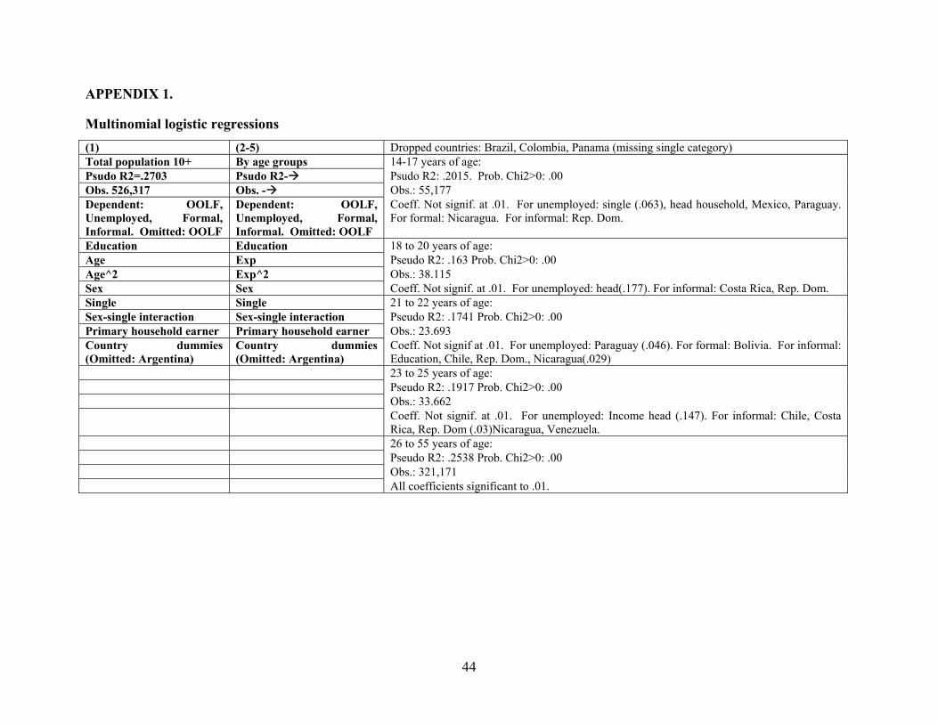
APPENDIX 1. Multinomial logistic regressions (1) (2-5) Dropped countries: Brazil, Colombia, Panama (missing single category) Total population 10+ By age groups 14-17 years of age: Psudo R2=.2703 Psudo R2- Psudo R2: .2015. Prob. Chi2>0: .00 Obs. 526,317 Obs. - Obs.: 55,177 Dependent: OOLF,Unemployed, Formal,Informal. Omitted: OOLF

Dependent: OOLF,Unemployed, Formal,Informal. Omitted: OOLF

Coeff. Not signif. at .01. For unemployed: single (.063), head household, Mexico, Paraguay. For formal: Nicaragua. For informal: Rep. Dom.

Education Education 18 to 20 years of age: Age Exp Pseudo R2: .163 Prob. Chi2>0: .00 Age^2 Exp^2 Obs.: 38.115 Sex Sex Coeff. Not signif. at .01. For unemployed: head(.177). For informal: Costa Rica, Rep. Dom. Single Single 21 to 22 years of age: Sex-single interaction Sex-single interaction Pseudo R2: .1741 Prob. Chi2>0: .00 Primary household earner Primary household earner Obs.: 23.693 Country dummies(Omitted: Argentina)

Country dummies(Omitted: Argentina)

Coeff. Not signif at .01. For unemployed: Paraguay (.046). For formal: Bolivia. For informal: Education, Chile, Rep. Dom., Nicaragua(.029)

23 to 25 years of age: Pseudo R2: .1917 Prob. Chi2>0: .00 Obs.: 33.662 Coeff. Not signif. at .01. For unemployed: Income head (.147). For informal: Chile, Costa Rica, Rep. Dom (.03)Nicaragua, Venezuela. 26 to 55 years of age: Pseudo R2: .2538 Prob. Chi2>0: .00 Obs.: 321,171 All coefficients significant to .01.

44

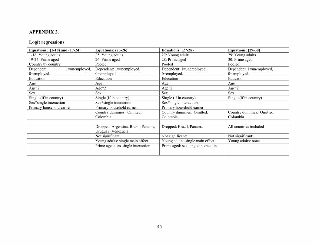
APPENDIX 2. Logit regressions Equations: (1-18) and (17-24) Equations: (25-26) Equations: (27-28) Equations: (29-30)1-18: Young adults 19-24: Prime aged Country by country

25: Young adults 26: Prime aged Pooled



Dependent: 1=unemployed,0=employed.

Dependent: 1=unemployed, 0=employed.



Education Education Education EducationAge Age Age AgeAge^2 Age^2 Age^2 Age^2Sex Sex Sex SexSingle (if in country) Single (if in country) Single (if in country) Single (if in country) Sex*single interaction Sex*single interaction Sex*single interaction Primary household earner Primary household earner Primary household earner Country dummies. Omitted:

Colombia. Country dummies. Omitted: Colombia.

Country dummies. Omitted: Colombia.

Dropped: Argentina, Brazil, Panama, Uruguay, Venezuela.

Dropped: Brazil, Panama All countries included

Not significant: Not significant: Not significant: Young adults: single main effect. Young adults: single main effect. Young adults: none Prime aged: sex-single interaction Prime aged: sex-single interaction

45

APPENDIX 3. Databases used

Argentina 1996 Ecuador 1995 Panama 1997 Bolivia 1997 Ecuador 1998 Peru 1997 Brazil 1996 Honduras 1998 Paraguay 1998 Chile 1996 Guatemala 1998 El Salvador 1995 Colombia 1997 Mexico 1996 El Salvador 1998 Costa Rica 1997 Nicaragua 1993 Uruguay 1997 Dominican Republic 1996 Nicaragua 1998 Venezuela 1997

APPENDIX 4. Wage and its Determinants: All Countries Dependent variable: lnwindex Independent variables: yedc (years of education); exp (expericence=age-6-yedc); exp2 (exp*exp); sexo (gender); lcoun_i (country i dummy). Icoun_18 is omitted Total population Age 14-17 Young adults Prime Age Number of obs. 429.501 18.488 88.464 279.273 AdjR-squared 0.3054 0.0897 0.1862 0.3045 Coef. P>|t| Coef. P>|t| Coef. P>|t| Coef. P>|t| yedc 0,134 - 0,131 - 0,136 - 0,134 - exp 0,042 - 0,032 0,00 0,032 - 0,028 - exp2 (0,000) - 0,004 - 0,001 - (0,000) - sexo 0,245 - 0,225 - 0,220 - 0,254 - Icoun_1 (0,245) - (0,184) - (0,265) - (0,226) - Icoun_2 (0,078) - 0,030 0,54 (0,059) 0,01 (0,048) - Icoun_3 0,316 - 0,110 - 0,190 - 0,384 - Icoun_4 (0,068) - 0,111 0,01 (0,148) - (0,076) - Icoun_5 0,057 - 0,232 - 0,092 - 0,048 - Icoun_6 0,109 - 0,192 - 0,157 - 0,088 - Icoun_7 (0,004) 0,74 (0,030) 0,60 (0,096) - (0,020) 0,13 Icoun_8 (0,166) - (0,136) 0,00 (0,202) - (0,134) - Icoun_9 0,130 - 0,598 - 0,380 - 0,005 0,67 Icoun_10 0,230 - (0,087) 0,03 0,101 - 0,332 - Icoun_11 0,123 - 0,014 0,71 0,035 0,03 0,182 - Icoun_12 0,392 - 0,300 - 0,290 - 0,406 - Icoun_13 (0,181) - (0,225) - (0,229) - (0,168) - Icoun_14 (0,208) - 0,197 0,00 (0,170) - (0,222) - Icoun_15 0,126 - 0,263 0,00 0,264 - 0,122 - Icoun_16 0,218 - 0,149 - 0,187 - 0,244 - Icoun_17 (0,229) - (0,396) - (0,319) - (0,204) - _cons 2,821 - 2,754 - 2,850 - 2,964 - Note: Countries are coded as follow (the number after the country indicates the year of the household survey): 1=Arg, 2=Bol, 3=Bra, 4=Chl, 5=Col, 6=Cri, 7=Dom, 8=Ecu, 9=Hon, 10=Gua, 11=Mex, 12=Nic, 13=Pan, 14=Per, 15=Pry, 16=Slv, 17=Ury and 18=Ven

46

APPENDIX 5. Wage and its Determinants: Regressions by Groups of Countries Dependent variable: ln(windex) Independent variables: yedc (years of education); exp (expericence=age-6-yedc); exp2 (exp*exp); sexo (gender), Lcoun_I (country dummy). Total population

Group 1 Group 2 Group 3 Group 4 Group 5 Group 6 Coef. Coef. Coef. Coef. Coef. Coef. Number of obs. 97.171 25.965 138.062 41.773 84.713 41.817 Adj. R-squared 0,255 0,191 0,425 0,230 0,312 0,239 yedc 0,115 0,124 0,161 0,111 0,130 0,114 exp 0,036 0,040 0,052 0,036 0,034 0,036 exp2 (0,000) (0,001) (0,001) (0,000) (0,000) (0,000) sexo 0,186 0,157 0,317 0,263 0,163 0,346 Icoun_4 0,165 Icoun_17 (0,001) Icoun_2 0,131 Icoun_8 0,035 Icoun_3 0,196 Icoun_13 (0,144) Icoun_18 (0,003) Icoun_5 (0,065) Icoun_6 (0,011) Icoun_10 0,110 Icoun_12 0,251 Icoun_16 0,100 _cons 2,848 2,832 2,576 3,050 3,153 3,115 Notes: Dark gray shading indicates that the variable is not significant at 10%. Light gray shading indicates that the variable is significant at 10%. All other variables are significant at 5%.

47

15 to 17 years old

Group 1 Group 2 Group 3 Group 4 Group 5 Group 6 Coef. Coef. Coef. Coef. Coef. Coef. Number of obs. 1.660 1.122 8.146 1.396 3.712 2.452 Adj. R-squared 0,084 0,020 0,148 0,062 0,049 0,172 yedc 0,094 0,015 0,147 0,159 0,123 0,143 exp 0,040 0,014 0,007 0,089 0,038 0,116 exp2 0,003 (0,000) 0,006 0,005 0,003 0,000 sexo 0,074 0,382 0,188 0,263 0,102 0,598 Icoun_4 0,287 Icoun_17 (0,206) Icoun_2 (0,235) Icoun_8 (0,416) Icoun_3 (0,143) Icoun_13 0,171 Icoun_18 0,209 Icoun_5 0,215 Icoun_6 0,185 Icoun_9 0,436 Icoun_10 (0,250) Icoun_12 0,063 _cons 2,931 3,804 3,013 2,112 2,897 2,348 Young adults Group 1 Group 2 Group 3 Group 4 Group 5 Group 6 Coef. Coef. Coef. Coef. Coef. Coef. Number of obs. 17.287 4.544 31.915 8.468 16.804 9.446 Adj. R-squared 0,144 0,064 0,286 0,141 0,205 0,155 yedc 0,120 0,121 0,162 0,117 0,128 0,119 exp 0,026 0,066 0,027 0,022 0,018 0,038 exp2 0,002 (0,001) 0,002 0,001 0,001 0,000 sexo 0,111 0,278 0,280 0,238 0,097 0,379 Icoun_4 0,121 Icoun_17 (0,055) Icoun_2 0,107 Icoun_8 (0,049) Icoun_3 (0,061) Icoun_7 0,121 Icoun_18 0,209 Icoun_5 0,053 Icoun_6 0,126 Icoun_9 0,267 Icoun_12 0,161 Icoun_16 0,087 _cons 2,809 2,717 2,865 2,828 3,127 2,995 Notes: Dark gray shading indicates that the variable is not significant at 10%. Light gray shading indicates that the variable is significant at 10%. All other variables are significant at 5%.

48

Prime age adults

Group 1 Group 2 Group 3 Group 4 Group 5 Group 6 Coef. Coef. Coef. Coef. Coef. Coef. Number of obs. 67.764 16.696 86.486 27.986 55.482 24.859 Adj. R-squared 0,239 0,195 0,405 0,209 0,331 0,258 yedc 0,118 0,127 0,160 0,111 0,133 0,111 exp 0,023 0,035 0,034 0,018 0,024 0,020 exp2 (0,000) (0,000) (0,000) (0,000) (0,000) (0,000) sexo 0,199 0,121 0,352 0,268 0,177 0,319 Icoun_4 0,144 Icoun_17 0,013 Icoun_2 0,088 Icoun_8 (0,086) Icoun_15 (0,254) Icoun_13 (0,118) Icoun_18 0,010 Icoun_5 (0,047) Icoun_11 0,092 Icoun_9 (0,390) Icoun_10 (0,057) Icoun_16 (0,147) _cons 2,966 2,945 3,008 3,242 3,200 3,639 Notes: Dark gray shading indicates that the variable is not significant at 10%. Light gray shading indicates that the variable is significant at 10%. All other variables are significant at 5%.

49

APPENDIX 6. Wage and its Determinants: Regressions by Country Dependent variable: ln(wage) Independent variables: yedc (years of education); exp (expericence=age-6-yedc); exp2 (exp*exp); sexo (gender). Total population ARG BOL BRA CHL COL CRI DOM ECU HON GUA MEX NIC PAN PER PRY SLV URY VEN

Coef. Coef. Coef. Coef. Coef. Coef. Coef. Coef. Coef. Coef. Coef. Coef. Coef. Coef. Coef. Coef. Coef. Coef.Number of obs. 29952 10173 136217 43824 50902 12744 8176 9374 10208 10635 21067 5832 11570 6418 1845 15142 23395 22077Adj R-squared 0,236 0,280 0,429 0,258 0,330 0,256 0,238 0,137 0,153 0,337 0,308 0,229 0,378 0,209 0,184 0,296 0,275 0,172yedc 0,098 0,129 0,161 0,127 0,133 0,107 0,096 0,119 0,082 0,138 0,137 0,125 0,128 0,127 0,135 0,112 0,115 0,107exp 0,041 0,038 0,052 0,031 0,028 0,028 0,040 0,049 0,008 0,055 0,049 0,037 0,042 0,029 0,026 0,042 0,042 0,032exp2 (0,001) (0,000) (0,001) (0,000) (0,000) (0,000) (0,000) (0,001) (0,000) (0,001) (0,001) (0,000) (0,000) (0,000) (0,000) (0,001) (0,000) (0,000)sexo 0,102 0,032 0,321 0,221 0,168 0,138 0,296 0,339 0,593 0,249 0,151 0,181 0,285 0,088 (0,044) 0,310 0,228 0,237_cons 3,083 3,031 2,765 2,875 3,140 3,396 3,080 2,707 3,579 2,864 2,914 3,336 2,651 2,947 3,445 3,186 2,765 3,160

Age 15-17

ARG BOL BRA CHL COL CRI DOM ECU HON GUA MEX NIC PAN PER PRY SLV URY VENCoef. Coef. Coef. Coef. Coef. Coef. Coef. Coef. Coef. Coef. Coef. Coef. Coef. Coef. Coef. Coef. Coef. Coef.

Number of obs. 604 375 8062 655 1933 735 250 564 728 713 1044 391 256 183 84 620 890Adj R-squared 0,010 0,214 0,147 0,029 0,039 0,045 0,111 0,008 0,138 0,065 0,054 0,087 0,092 0,001 0,042 0,179 0,011 0,041yedc 0,076 0,089 0,147 0,116 0,105 0,134 0,189 (0,077) 0,176 0,111 0,153 0,099 0,180 0,047 0,133 0,154 0,109 0,149exp 0,063 (0,046) 0,008 (0,022) 0,028 0,028 0,247 0,038 0,164 (0,017) 0,045 0,081 0,165 0,067 (0,067) 0,155 0,116 0,030 exp2 (0,002) 0,007 0,006 0,011 0,002 0,007 (0,006) (0,003) 0,000 0,009 0,006 (0,003) (0,000) (0,007) 0,014 (0,000) (0,003) 0,009 sexo 0,078 0,606 0,190 0,108 0,118 0,183 0,451 0,285 0,990 0,338 0,034 0,404 0,342 0,028 (0,049) 0,552 0,030 0,187 _cons 3,052 3,039 2,868 3,115 3,285 2,931 1,570 4,020 2,161 2,759 2,670 3,081 1,740 3,739 3,383 2,181 2,511 2,590

401

Notes: Dark gray shading indicates that the variable is not significant at 10%. Light gray shading indicates that the variable is significant at 10%. All other variables are significant at 5%.

50

Young adults


Number of obs. 5235 1581 31588 7861 9617 2650 1724 1798 2428 2183 4537 1228 2263 1165 327 3607 4191 4481Adj R-squared 0,136 0,194 0,286 0,139 0,221 0,176 0,147 0,029 0,069 0,260 0,191 0,156 0,211 0,105 0,210 0,218 0,131 0,112yedc 0,112 0,124 0,162 0,124 0,123 0,107 0,101 0,121 0,053 0,174 0,145 0,118 0,133 0,119 0,148 0,127 0,126 0,118exp 0,045 0,015 0,027 (0,011) (0,002) 0,002 0,040 0,100 0,008 0,047 0,057 0,010 0,026 0,071 (0,018) 0,054 0,068 0,013 exp2 0,001 0,001 0,002 0,004 0,002 0,002 0,001 (0,003) (0,001) 0,001 0,000 0,001 0,002 (0,003) 0,003 0,000 (0,000) 0,002 sexo 0,018 0,313 0,280 0,169 0,090 0,098 0,268 0,392 0,558 0,256 0,107 0,311 0,290 0,041 0,276 0,351 0,124 0,206_cons 2,877 2,957 2,802 2,981 3,339 3,479 3,008 2,424 3,893 2,512 2,747 3,394 2,600 2,903 3,207 2,922 2,529 3,104

Prime age


Number of obs. 21650 6744 85353 30616 34224 8182 5232 5707 5953 6166 13076 3539 8133 4245 1133 9201 15498 14621Adj R-squared 0,199 0,261 0,408 0,262 0,351 0,258 0,198 0,145 0,171 0,322 0,313 0,217 0,359 0,218 0,179 0,292 0,245 0,154yedc 0,097 0,130 0,160 0,134 0,137 0,106 0,094 0,119 0,088 0,128 0,137 0,123 0,131 0,137 0,133 0,110 0,115 0,105exp 0,032 0,040 0,034 0,016 0,024 0,011 0,019 0,051 0,009 0,028 0,031 0,022 0,028 (0,001) (0,003) 0,019 0,026 0,009exp2 (0,000) (0,001) (0,000) 0,000 (0,000) (0,000) (0,000) (0,001) (0,000) (0,000) (0,000) (0,000) (0,000) 0,000 0,000 (0,000) (0,000) 0,000 sexo 0,116 (0,035) 0,356 0,238 0,182 0,157 0,299 0,317 0,529 0,268 0,165 0,147 0,275 0,097 (0,083) 0,279 0,236 0,256_cons 3,210 3,054 3,000 2,940 3,114 3,625 3,352 2,741 3,531 3,359 3,149 3,596 2,740 3,089 3,864 3,507 2,999 3,462


51

APPENDIX 7. Wage and its Determinants: Regressions by Country Dependent variable: ln(wage) Independent variables: yedc (years of education); splin# (spline variable); exp (expericence=age-6-yedc); exp2 (exp*exp); sexo (gender).

All population ECU HON GUA MEX PAN PRY SLV URY CRI NIC PER VEN ARG BRA DOM BOL COL CHIAll Coef. Coef. Coef. Coef. Coef. Coef. Coef. Coef. Coef. Coef. Coef. Coef. Coef. Coef. Coef. Coef. Coef. Coef.Number of obs.

9.374 10.208 10.635 21.067 11.570 1.845 15.142 23.395 12.744 5.832 6.418 22.027 29.952 136.217 8.176 10.173 50.902 43.824

Adj R-squared

0.140 0.154 0.346 0.313 0.388 0.193 0.312 0.281 0.272 0.234 0.215 0.183 0.244 0.438 0.255 0.287 0.337 0.282

yedc 0.087 0.064 0.088 0.096 0.063 0.087 0.074 0.066 0.062 0.103 0.079 0.066 0.050 0.146 0.078 0.115 0.106 0.067splin2a (0.005) 0.007 0.050 0.049 0.062 0.077 0.006 0.040 0.026 0.035 0.059 0.019 0.024 (0.027) (0.023) 0.007 0.013 0.007 splin3a 0.078 0.036 0.127 0.082 0.065 0.045 0.100 0.035 0.039 (0.016) 0.004 0.058 0.064 0.034 0.004 (0.031) 0.012 0.056splin4a 0.043 0.048 0.056 0.040 0.095 0.148 0.100 0.089 0.111 0.097 0.098 0.103 0.074 0.084 0.093 0.112 0.078 0.142exp 0.049 0.007 0.054 0.050 0.045 0.027 0.041 0.043 0.028 0.037 0.030 0.034 0.042 0.050 0.039 0.035 0.028 0.033exp2 (0.001) (0.000) (0.001) (0.001) (0.001) (0.000) (0.001) (0.001) (0.000) (0.000) (0.000) (0.000) (0.001) (0.001) (0.000) (0.000) (0.000) (0.000)sexo 0.347 0.590 0.268 0.165 0.291 (0.017) 0.325 0.231 0.140 0.174 0.110 0.243 0.113 0.321 0.302 0.049 0.164 0.232 _cons 6.420 1.515 (0.116) 0.010 (1.416) 6.432 0.576 1.524 4.584 0.027 (0.754) 4.865 (0.362) (1.419) 1.232 (0.385) 5.514 4.955Notes: Dark gray shading indicates that the variable is not significant at 10%. Light gray shading indicates that the variable is significant at 10%. All other variables are significant at 5%.

52

Age 15-17

ECU HON GUA MEX PAN PRY SLV URY CRI NIC PER VEN ARG BRA DOM BOL COL CHICoef. Coef. Coef. Coef. Coef. Coef. Coef. Coef. Coef. Coef. Coef. Coef. Coef. Coef. Coef. Coef. Coef. Coef.

Number of obs.

564 728 713 1,044 256 84 620 401 735 391 183 890 604 8,062 250 375 1,933 655

Adj R-squared

0.008 0.137 0.066 0.053 0.115 0.021 0.179 0.009 0.044 0.088 0.002 0.040 0.013 0.147 0.121 0.215 0.041 0.031

yedc 0.030 0.175 0.087 0.140 0.007 0.077 0.174 0.032 0.119 0.118 0.033 0.120 0.049 0.154 0.285 0.184 0.083 0.124 splin2a (0.100) 0.051 0.100 0.020 0.301 0.089 (0.055) 0.103 0.012 (0.116) (0.057) 0.054 0.077 (0.017) (0.084) (0.117) 0.082 (0.079) splin3a (0.399) (0.699) (0.003) 0.108 0.123 0.055 (0.205) 0.073 0.146 0.156 0.166 0.059 (0.285) 0.017 (0.255) (0.143) (0.034) 0.063 splin4a (droppe

d) (dropped)

(dropped)

(dropped)

(dropped)

(dropped)

(dropped)

(dropped)

(dropped)

(dropped)

(dropped)

(dropped)

(dropped)

(dropped)

(dropped)

(dropped)

(dropped)

(dropped)

exp (0.063) 0.165 0.028 0.057 0.346 (0.024) 0.129 0.164 0.052 0.042 0.084 0.072 0.098 0.002 0.140 (0.114) 0.057 (0.024) exp2 0.012 (0.000) 0.004 0.005 (0.025) 0.007 0.003 (0.011) 0.003 0.000 (0.011) 0.004 (0.007) 0.006 0.007 0.017 (0.001) 0.011 sexo 0.297 0.990 0.352 0.034 0.332 (0.037) 0.551 0.031 0.188 0.411 0.062 0.187 0.090 0.191 0.452 0.608 0.110 0.105 _cons 7.083 0.009 (0.378) (0.347) (2.026) 6.425 (0.624) 1.342 3.911 (0.283) (0.093) 4.154 (0.609) (1.457) (0.634) (0.821) 5.510 4.834


53

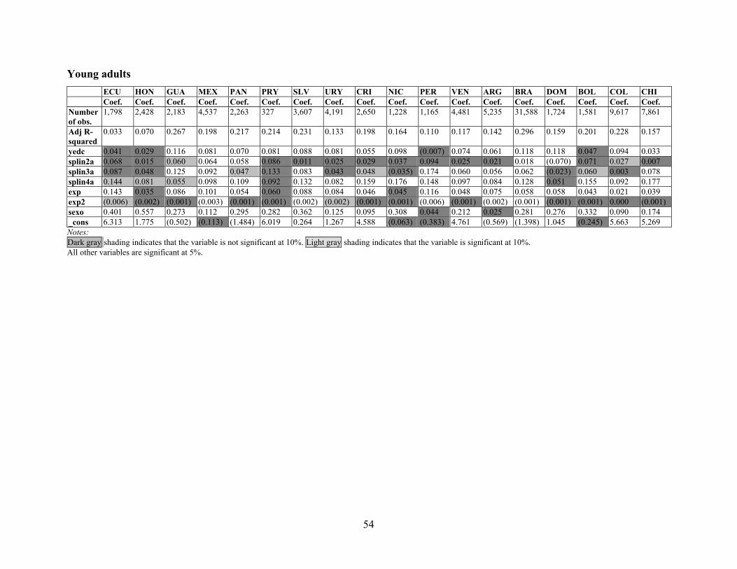
Young adults

ECU HON GUA MEX PAN PRY SLV URY CRI NIC PER VEN ARG BRA DOM BOL COL CHICoef. Coef. Coef. Coef. Coef. Coef. Coef. Coef. Coef. Coef. Coef. Coef. Coef. Coef. Coef. Coef. Coef. Coef.

Number of obs.

1,798 2,428 2,183 4,537 2,263 327 3,607 4,191 2,650 1,228 1,165 4,481 5,235 31,588 1,724 1,581 9,617 7,861

Adj R-squared

0.033 0.070 0.267 0.198 0.217 0.214 0.231 0.133 0.198 0.164 0.110 0.117 0.142 0.296 0.159 0.201 0.228 0.157

yedc 0.041 0.029 0.116 0.081 0.070 0.081 0.088 0.081 0.055 0.098 (0.007) 0.074 0.061 0.118 0.118 0.047 0.094 0.033splin2a 0.068 0.015 0.060 0.064 0.058 0.086 0.011 0.025 0.029 0.037 0.094 0.025 0.021 0.018 (0.070) 0.071 0.027 0.007 splin3a 0.087 0.048 0.125 0.092 0.047 0.133 0.083 0.043 0.048 (0.035) 0.174 0.060 0.056 0.062 (0.023) 0.060 0.003 0.078 splin4a 0.144 0.081 0.055 0.098 0.109 0.092 0.132 0.082 0.159 0.176 0.148 0.097 0.084 0.128 0.051 0.155 0.092 0.177exp 0.143 0.035 0.086 0.101 0.054 0.060 0.088 0.084 0.046 0.045 0.116 0.048 0.075 0.058 0.058 0.043 0.021 0.039exp2 (0.006) (0.002) (0.001) (0.003) (0.001) (0.001) (0.002) (0.002) (0.001) (0.001) (0.006) (0.001) (0.002) (0.001) (0.001) (0.001) 0.000 (0.001) sexo 0.401 0.557 0.273 0.112 0.295 0.282 0.362 0.125 0.095 0.308 0.044 0.212 0.025 0.281 0.276 0.332 0.090 0.174 _cons 6.313 1.775 (0.502) (0.113) (1.484) 6.019 0.264 1.267 4.588 (0.063) (0.383) 4.761 (0.569) (1.398) 1.045 (0.245) 5.663 5.269


54

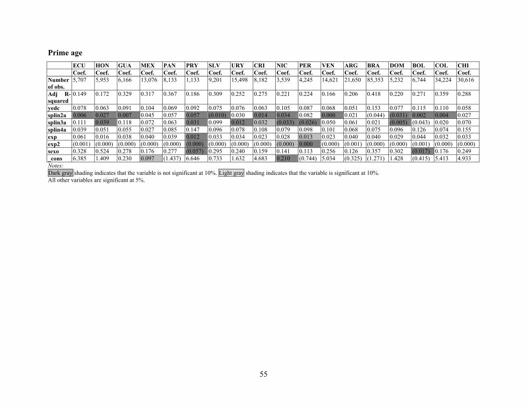
Prime age ECU HON GUA MEX PAN PRY SLV URY CRI NIC PER VEN ARG BRA DOM BOL COL CHI

Coef. Coef. Coef. Coef. Coef. Coef. Coef. Coef. Coef. Coef. Coef. Coef. Coef. Coef. Coef. Coef. Coef. Coef.Number of obs.

5,707 5,953 6,166 13,076 8,133 1,133 9,201 15,498 8,182 3,539 4,245 14,621 21,650 85,353 5,232 6,744 34,224 30,616

Adj R-squared

0.149 0.172 0.329 0.317 0.367 0.186 0.309 0.252 0.275 0.221 0.224 0.166 0.206 0.418 0.220 0.271 0.359 0.288

yedc 0.078 0.063 0.091 0.104 0.069 0.092 0.075 0.076 0.063 0.105 0.087 0.068 0.051 0.153 0.077 0.115 0.110 0.058splin2a 0.006 0.027 0.007 0.045 0.057 0.057 (0.010) 0.030 0.014 0.034 0.082 0.000 0.021 (0.044) (0.031) 0.002 0.004 0.027 splin3a 0.111 0.039 0.118 0.072 0.063 0.031 0.099 0.012 0.032 (0.033) (0.026) 0.050 0.061 0.021 (0.005) (0.043) 0.020 0.070splin4a 0.039 0.051 0.055 0.027 0.085 0.147 0.096 0.078 0.108 0.079 0.098 0.101 0.068 0.075 0.096 0.126 0.074 0.155exp 0.061 0.016 0.038 0.040 0.039 0.012 0.033 0.034 0.023 0.028 0.013 0.023 0.040 0.040 0.029 0.044 0.032 0.033exp2 (0.001) (0.000) (0.000) (0.000) (0.000) (0.000) (0.000) (0.000) (0.000) (0.000) 0.000 (0.000) (0.001) (0.000) (0.000) (0.001) (0.000) (0.000)sexo 0.328 0.524 0.278 0.176 0.277 (0.057) 0.295 0.240 0.159 0.141 0.113 0.256 0.126 0.357 0.302 (0.017) 0.176 0.249 _cons 6.385 1.409 0.230 0.097 (1.437) 6.646 0.733 1.632 4.683 0.210 (0.744) 5.034 (0.325) (1.271) 1.428 (0.415) 5.413 4.933


55

Adolescents and Young Adults in Latin America, Critical Decisions at a Critical Age: Young Adult...

Documents

Transcript of Adolescents and Young Adults in Latin America, Critical Decisions at a Critical Age: Young Adult...