Electronic copy available at: http://ssrn.com/abstract=1824390

Addressing Onsite Sampling in Recreation Site Choice Models

Paul Hindsley,1* Craig E. Landry,2 and Brad Gentner3

1Environmental Studies, Eckerd College, St. Petersburg, FL 33711 hindslpr@eckerd.edu 2 Department of Economics, East Carolina University, Greenville, NC 27858 landryc@ecu.edu

3Gentner Consulting Group, Silver Spring, MD 20901 brad@gentnergroup.com

Abstract

Independent experts and politicians have criticized statistical analyses of recreation behavior that rely upon onsite samples due to their potential for biased inference, prompting some to suggest support for these efforts should be curtailed. The use of onsite sampling usually reflects data or budgetary constraints but can lead to two primary forms of bias in site choice models. First, the strategy entails sampling site choices rather than sampling anglers– a form of bias called endogenous stratification. Under these conditions, sample choices may not reflect the site choices of the true population. Second, the exogenous attributes of the recreational users sampled onsite may differ from the attributes of users in the population – the most common form in recreation demand is avidity bias. We propose addressing these biases by combining two existing methods, Weighted Exogenous Stratification Maximum Likelihood Estimation (WESMLE) and propensity score estimation. We use the National Marine Fisheries Service’s (NMFS) Marine Recreational Fishing Statistics Survey (MRFSS) to illustrate methods of bias reduction employing both simulation and empirical applications. We find that propensity score based weights can significantly reduce bias in estimation. Our results indicate that failure to account for these biases can overstate anglers’ willingness to pay for additional fishing catch. Key words: On-site sampling, propensity score weighting, recreation demand, random

utility models

* Corresponding Author.

Special thanks to John Whitehead, Haiyong Liu, George Parsons, Matt Massey, and numerous attendees at Camp Resources for their helpful comments.

Electronic copy available at: http://ssrn.com/abstract=1824390

Addressing Onsite Sampling in Recreation Site Choice Models

Introduction

Independent experts (CIE 2006; NRC 2006) and politicians (Sergeant 2010) have

noted the inherent bias associated with onsite sampling, leading some to conclude that

federal expenditures should be curtailed until unbiased methods can be devised. Senator

Charles Schumer’s recent criticism of the NOAA’s MRFSS is a noteworthy example. In

studies of recreation behavior, budgetary constraints and data availability often influence

analysts’ choice of sampling strategy. Ideally, samples of recreational users would be

drawn from either simple random samples or exogenously stratified random samples. In

the both cases, common problems, such as non-response bias, can be relatively easy to

address using existing econometric procedures. Unfortunately, it is not always feasible to

use these sampling strategies. Sometimes budgetary or other practical constraints

necessitate the use of inherently biased sampling procedures. In the case of recreation

site choice models, researchers often utilize sampling strategies which target users onsite

through the implementation of intercept surveys. Onsite sampling strategies can entail

lower implementation costs, allow researchers to target resource users, and permit over-

sampling of rare choice patterns that may be of interest.

Statistical methods which utilize onsite samples must account for bias stemming

from non-random sampling (i.e. sample selection bias). In the application of random

utility models (RUMs) to recreation choice, respondents in onsite samples often represent

users with different characteristics than what is found in the “true” recreation population.

This difference can stem from two sources. First, when a sample is collected onsite, the

sample suffers from a type of non-ignorable sample selection bias, where the probability

1

of inclusion in the sample is simultaneously determined with the probability an individual

chooses a site – a process commonly termed endogenous stratification.1 This occurs

because the endogenously stratified sample draws observations from potential choices

and then observes the individuals that make those choices. The second type of bias is

directly connected to size-biased sampling – a type of bias previously identified in

ecology (Patil and Rao 1978) and single-site recreation demand models (Shaw 1988;

Englin and Shonkwiler 1996). When a sample is collected onsite, more avid recreational

users have a higher probability of being sampled than less avid recreational users.2 When

avidity bias occurs in a sample, statistical inferences are more heavily influenced by avid

users, thus failing to meet the requirements of randomness in the sample.

The primary objective of this paper is to provide a clear explanation of the

potential consequences of onsite sampling in site choice models and to convey an

approach for consistent estimation with maximum likelihood methods. We do this by

combining two existing econometric methods, Weighted Exogenous Stratification

Maximum Likelihood (WESML) estimation and propensity score estimation. The

propensity score procedure used herein is more commonly applied in balancing equations

for matching estimation; we use an auxiliary sample, which represents our angler

population, to develop a weight which “quasi-randomizes” the onsite sample. We apply

this joint weighting strategy to address sample selection bias in the National Marine

Fisheries Service’s (NMFS) Marine Recreational Fishing Statistics Survey (MRFSS).

We begin by creating a sample from an existing MRFSS dataset where we simulate an

onsite sampling procedure. We then compare weighted estimation routines using the

1 In RUMs, a sample with endogenous stratification is often called a choice-based sample. 2 Avidity refers to trip frequency. A more avid user has a higher trip frequency than a less avid user.

2

simulated data to routines using the original dataset. We follow this approach by again

estimating a site choice model using the MRFSS data, but now using weights estimated

from a random digit dial (RDD) sample of coastal households.

Our empirical results indicate that onsite sample selection within the MRFSS

leads to upward bias for estimates of anglers’ marginal willingness-to-pay for changes in

catch rates. The bias is not due simply to endogenous stratification, as estimates improve

with the application of propensity-score based weights that are devised to address avidity

bias, as well as differences in other exogenous attributes, in the onsite sample. While

propensity score estimation has been previously applied to weight estimation (Nevo

2002), we are unaware of any similar applications with Random Utility Models. Our

findings indicate that this method provides empirical researchers a viable option for bias

reduction when suitable auxiliary information is available.

Identifying and Correcting Bias from Onsite Sampling

The following description of sampling design for studies of recreation demand

draws heavily from a wide variety of previous works which focus on endogenous

stratification in discrete choice models (Manski and Lerman 1977; Manski and

McFadden 1981; Cosslett 1981a; Hsieh, Manski, and McFadden 1985; and Bierlaire,

Bolduc, and McFadden 2008) and onsite sampling in recreation demand models (Shaw

1988; Englin and Shonkwiler 1996; and Moeltner and Shonkwiler 2005). A rich

literature exists in relation to these topics, but the recreation demand literature lacks a

well defined explanation of the implications of sample selection bias as it relates to the

estimation of site choice models.

3

Onsite samples, otherwise known as intercept samples, suffer from two separate

types of sample selection bias, endogenous stratification and size-biased sampling.

Endogenous stratification occurs when an endogenous variable is part of a stratified

sample selection process. Size-biased sampling occurs when the probability of selection

is a function of the size of one or more exogenous sample characteristics. In recreation

demand, size-biased sampling confounds estimates in the form of avidity bias. Other

works in the recreation demand literature either address bias resulting from just

endogenous stratification in site choice models (Haab and McConnell 2003) or address

endogenous stratification in choice models indirectly by accounting for size-based

sampling bias in a multivariate setting via recreation users’ repeated choices (Moeltner

and Shonkwiler 2005). In this study, we describe these potential biases from the

perspective of general stratified sampling strategies (Manski and McFadden 1981;

Bierlaire, Bolduc, McFadden 2008) and propose one potential method which reduces this

bias in a cross-sectional setting through the use of auxiliary information.

The distribution of recreation choices can be represented via a joint probability

density function, , where each user makes a choice (i) from a finite and exhaustive

set of recreation sites ( ). The exogenous attributes of these choices (z) are

composed of the demographic characteristics of the decision makers and the attributes of

alternatives. The exogenous attributes are elements of an exhaustive set that occurs in the

population (

),( zif

i C∈

Zz∈ ). This joint distribution is the set of all possible combinations of

endogenous and exogenous attributes, which can be depicted as ZCzif ×∈),( .

In the model of interest, we have two important processes: 1) the probability that

an individual is sampled from the population, and 2) the probability that an individual

4

makes a choice, given exogenous attributes. Ideally, sample selection is exogenous to the

choice process. When the probability of selection is endogenous to the choice process,

the estimation procedure will suffer from a form of non-ignorable sample selection bias

(Little and Rubin 1987). When this type of bias occurs as part of a stratified sampling

strategy, it is referred to as endogenous stratification (Manski and McFadden 1981).

For our purposes, it is useful to represent the joint density of site choices as:

)(),|(),Pr( zpziPzi β= (1)

where ),|( βziP represents the choice model of interest - probability of site choice

conditional on exogenous attributes and a vector of unknown parametersβ , and

represents the marginal distribution of exogenous attributes in the population. If a simple

random sample is drawn from , the kernel in equation (1)

)(zp

),( zif ),|( βziP , provides a

basis for estimation of the unknown parameters, β .3 Under a stratified sampling

strategy, the population is partitioned into groups or strata ( S,...,s 1= ) according to either

exogenous or endogenous factors. Let Rs(i, z) be the qualification probability,

determining whether an element of may be included in strata s. Note that Rs(i, z)

can be a function of exogenous attributes, endogenous attributes, or both. If the

endogenous attributes affect the qualification probability, then the unknown parameters

do as well.

), zi(f

The conditional site choice distribution given qualification is:

∫∑∈

=

z Cjs

s

dzzpzjPzjRzpziPziR

sziG)(),|(),(

)(),|(),()|,(

ββ

, (2)

3 The marginal distribution of exogenous attributes, , is ancillary and can be conditioned out of the likelihood function.

)(zp

5

where the denominator is the qualification factor that identifies the proportion of the

population qualifying for stratum s. Unlike a simple random sample, the generalized

conditional distribution in (2) depends upon the unknown parameter vector β and the

distribution of exogenous explanatory variables p(z) (McFadden 1999). If the sample is

only exogenously stratified, the qualification factor simplifies to , which is

independent of β. In this case, the kernel is independent of the stratification structure,

and the sampling strategy can be ignored in estimation of β, but must be taken into

account in estimation of asymptotic standard errors. With an onsite sample, stratification

can be influenced by both endogenous and exogenous factors, in which case there is no

such simplification.

∫z

s dzzpzR )()(

Let n(i, z | s) represent the number of observations in stratum s with observed

variables (i, z). The log-likelihood function for the stratified sample is then:

∑∑∑=

=S

s z isziGszinLL

1)|,(ln)|,()(β . (3)

Consistent estimation can be achieved with a pseudo-maximum likelihood approach.

Weighted Exogenous Sample Maximum Likelihood (WESML) estimation utilizes the

log-likelihood function:

∑∑∑=

=S

s z i

ziPsziwszinLL1

),|(ln),,()|,()( ββ , (4)

where w(i, z, s) is a weight that adjusts for stratification.4 With a sample that is only

endogenously stratified (i.e. pure choice-based sample – so that s = i), the appropriate

weight is the ratio of the population to the sample frequency:

4 An alternative approach to address endogenous stratification in RUM is Conditional Maximum Likelihood (CML) (Manski and McFadden 1981). CML involves pooling observations across strata, and

6

) (5) (/)(),( iHiQsiw ss=

where the weight, ,equals the population proportion of recreational choices i for

strata s, , divided by the sample proportion of recreational choices, i, for each strata

s, . This estimator can be applied if the sample is collected onsite, but the

researcher can be sure that the sample is randomized within a particular site. In this case,

a specific choice may be oversampled, but the individuals making that choice would be

representative of the larger population.

),( siw

)(iQs

)(is

)(iH s

ˆ

5 While Manski and Lerman’s (1977) application

of this weight obtains the sample share, , via the sampling process, it is assumed

that the population share, , is known by the analyst a priori. In Cosslett’s (1981)

application, the weight, , utilizes an estimate of the population share in a given

strata,Q , which replaces the known population share, , in the the pseudo-

likelihood estimator.

)(iH s

)(iQs

),( siw

)(iQs

With both endogenous and exogenous stratification, one can reweight

observations for both factors, producing the weight:

),(/),(),,( ziHziQsziw ss= , (6)

where is the joint probability of choices and exogenous attributes within a given

strata for the population and is the joint probability of choices and exogenous

),( ziQs

),( ziH s

then forming the likelihood of i conditional on z in the pool, which conditions out p(z). Hsieh, Manski, and McFadden (1985) show that CML is a more efficient estimator than WESML, but in recreation demand modeling this added efficiency may come at the expense of additional computational burden. When individuals are faced with a high number of alternative choices, the CML model suffers from the burden of dimensionality. Under these conditions, the decreased computational burden of WESML often outweighs any loss of efficiency. 5 For example, consider the case of a discrete support for z. On a contingency table for f(i, z), with C columns and Z rows, pure choice-based sampling implies that a specific column is over-sampled, but the proportion of cells in that column, which represent all the exogenous characteristics of individuals making that choice, match the proportion found in the population (Manski and McFadden 1981).

7

attributes within a given strata for the sample. The expressions in equations (5) and (6)

are inverse-probability weights that reweight observations in inverse proportion to the

probability with which they qualify from the population. Wooldridge (2002) shows that

inverse probability weights can be used to address sample selection bias within the

general class of M-estimators (which includes linear and nonlinear regression, count data

models, and discrete choice models). In most scenarios, the joint probability of choices

and exogenous attributes for the population, , will be unknown, necessitating an

estimate, .

),( ziQs

),(ˆ ziQs

Methods

We propose to use propensity score based weights to address biases resulting from

exogenous and endogenous stratification in recreation site choice models. The propensity

score refers to the conditional probability of assignment to a particular treatment given a

vector of covariates (Rosenbaum and Rubin 1983). This can either be known a priori or

estimated using auxiliary information. Recent studies have shown that propensity scores

can be used in both matching and selection models to address choice-based sampling.6 In

an empirical application, Nevo (2003) adjusts for non-ignorable sample selection using

inverse probability weights estimated from an auxiliary sample.

The propensity score acts as a balancing factor, b(i,z,s), which renders the

conditional distribution of choices, i, and observed covariates, z, the same for treated (t =

1) and control (t = 0) groups: g(i,z,s | b(i,z,s), t = 1) = g(i,z,s| b(i,z,s) , t = 0) (Rosenbaum

and Rubin 1983). The weighting procedure allows the onsite sample to be treated as

6 See Heckman and Navarro 2004 for a discussion of the different roles for propensity scores.

8

‘quasi-randomized’.7 Previous studies have shown that estimated weights may improve

efficiency relative to estimation procedures using known weights (Cosslett 1981; Hirano,

Imbens, and Ridder 2003). Because our sample selection bias is of a non-ignorable form,

the propensity score must reflect endogenous choice, i , and exogenous characteristics, z ,

for each individual. We assign our onsite sample to the control group (t = 0) and our

random sample to the treatment group (t = 1). We then estimate a weight which will

randomize our control group. This method attempts to alter the distribution of strata,

which are based on choices and exogenous factors, so that the joint distribution of onsite

observations matches the joint distribution of the random sample. Ridgeway (2006)

describes the basic decomposition of the weight as follows:

)0|,,(),,()1|,,( === tszigsziwtszig (7)

where is a weight that equilibrates the joint distributions of for the two

samples. Ridgeway shows that by solving for and applying Bayes’ Theorem to

the conditional distributions of , one obtains:

),,( sziw ),,( szi

),,( sziw

),,( szi

),,|1(1),,|1(),,(szitg

szitgKsziw=−

== . (8)

In this weight, the constant K cancels out in the estimation of the choice model. This

weight has the form:

),,Pr(1),,Pr(

szisziw −= , (9)

and represents the odds that that an angler sampled onsite with features would be a

member of the random sample (the treatment). McCaffrey, Ridgeway, and Morral (2004)

),( zi

7 It is quasi-randomized instead of randomized because the process only accounts for observed differences. There is always the risk that unobserved differences exist.

9

describe the denominator of this weight as accounting for the over sampling of

individuals in the onsite sample and weighting the pooled sample into a collection of

anglers sampled both randomly and onsite. The numerator of this equation weights the

joint distribution of the choices, exogenous factors and strata , in this pooled

sample to match the joint distribution of in the random sample, represented by

. We interpret this as an inverse probability weight because the probability of

inclusion in the onsite sample, depicted by

),,( szi

),,( szi

Pr(1(

),,Pr( szi

)),, szi− , occurs in the denominator of

the weight while inclusion in the population, , occurs in the numerator. ),, szi

)),, szi

Pr(

Pr(1log(

For estimation purposes, we utilize a form of the Bernoulli log-likelihood

function:

)1(),,Pr(log(Pr) tszitLL −−+= . (10)

We take a logistic transformation of so that each estimated probability is

confined to the unit interval. The logistic transformation is:

),, sziPr(

,,(exp(11),,|1

zigszit

−+==Pr(

(ig

, (11) ))s

where represents some functional form for . When is a linear

combination of choices, i , exogenous factors,

),, sz )s,,( zi ),,( szig

z , and strata, s, equation (11) is a linear

logistic regression.

We propose using equation (11) as a first stage regression that estimates

propensity scores via equation (9) that feed into the likelihood function in (4). We let

include a combination of linear, higher-order, and interacted covariates so to

obtain an ignorable treatment assignment (Dehejia and Wahba 2002). The linear, higher-

),,( szig

10

order, and interacted covariates account for non-linear differences in endogenous and

exogenous attributes between the sample and the population.

One issue that must be addressed involves the selection of variables for the

estimation of the propensity score. In practice, the functional form of the propensity

score model is not known, necessitating a decision rule for variable selection. The

propensity score has no behavioral assumptions, as it only acts to reduce the dimensions

of conditioning. There are numerous estimators and variable selection methods available

for propensity score estimation. The logit and probit models are the most commonly

applied method for propensity score estimation but both require a method for variable

selection. Dehejia and Wahba (2002) and Hirano and Imbens (2001) provide methods for

variable selection when using parametric estimation procedures such as the probit and

logit regression models. We choose to focus on a flexible, nonparametric application

proposed by McCaffrey, Ridgeway, and Morral (2004) called the generalized boosted

model (GBM).8

McCaffrey, Ridgeway, and Morral (2004) describe the GBM as an algorithm that

is general, automated, and adaptive in prediction. GBM allows models to be specified

with large numbers of covariates in a nonlinear fashion. In a more general discussion,

Friedman, Hastie, and Tibshirani (2000) define boosting models as committee methods

which combine numerous simple functions (weak classifiers) to estimate one smooth

function.9 Each of the simple functions may lack the necessary characteristics to

8 We estimated numerous propensity score models, including those proposed by Dehejia and Wahba (2002) and Hirano and Imbens (2001). In our applications we found GBM outperformed the alternative choices. We choose this estimator not only because of its precision, but because it is also readily available in the open-source software package R (R Core Development, 2009). 9 Hastie et al. define a weak classifier as a classifier that has an error rate only slightly better than random guessing.

11

adequately approximate the function of interest, but when combined as a committee, the

combination of simple functions “can approximate a smooth function just like a sequence

of line segments can approximate a smooth curve” (McCaffrey, Ridgeway, and Morral

2004).10

Using GBM, we estimate the propensity score by maximizing the Bernoulli

likelihood from equation (10), where the joint distribution of endogenous and exogenous

factors, as well as strata ( ), are represented by a probability model with a logistic

functional form, as seen in equation (11).

),,( szig

11 The GBM algorithm adaptively fits the form

of , thus taking advantage of the boosting procedures’ bias and variance

reduction properties while still employing a common logistic functional form.

),,( szig

The GBM algorithm initiates by setting the log odds to a constant value, which, in

our application, is equal to the log of the average number of observations in the RDD

sample divided by the average number in the intercept sample, represented by

( )tt−1log . The algorithm then iteratively works to improve upon this baseline estimate

by adjusting the logit functional form by a factor ),,( szihλ such that:

))),,(ˆ(())),,(),,(ˆ(( szigLLEszihszigLLE >+ λ , (12)

Each iteration contributes a small adjustment, ),,( szihλ which updates the current

estimate of such that ),,(ˆ szigk

),,(),,(ˆ),,(ˆ 1 szihszigszig kkk λ+←+ (13)

where k represents the current iteration, and k + 1 represents the updated estimate.

10 For a more thorough introduction to boosting, see Hastie, Tibshirani, and Friedman (2001) or McCaffrey, Ridgeway, and Morral (2004). This description relies heavily on those works. 11 GBM estimates this probability through a generalized iteratively reweighted least squares algorithm.

12

GBM iteratively improves estimation by finding a local improvement in the likelihood

function, based on its gradient. Friedman (2001) found that the residual of the expected

log-likelihood contains information on this improvement. The residual is simply the

difference between the treatment indicator and the probability of treatment. GBM then

uses a regression tree algorithm (Breiman et al 1984) to find a piecewise constant

function of the covariates, , that captures correlations with the residuals. The

adjustment contains information pertaining to those values of i ,

),,( szih

z and s which

adequately fit the model. The GBM algorithm then uses the adjustment to update the log

likelihood function, as seen in equation 12. Each iteration of the algorithm then utilizes a

line search to find the coefficientλ with the greatest increase in the log likelihood.

As the number of iterations rise, the complexity of the model also increases.

Ridgeway (2006) describes this as a bias/variance tradeoff where, with additional

iterations, the reduction of bias comes at the expense of increasing variance. The GBM

catalogs a set of propensity scores - one for each iteration. Before running the algorithm,

the analyst determines the total number of iterations to run. After running all the

iterations, the optimal set of propensity scores are chosen using a predetermined set of

selection rules. For the GBM package, one such guideline is finding the smallest average

effect size difference across covariates between the treatment and comparison groups

(Ridgeway 2007a).

We represent saltwater recreational angler choice through the application of the

Random Utility Maximization (RUM) model. Under the assumption that saltwater

recreational anglers engage in utility maximizing behavior, random utility models allow

13

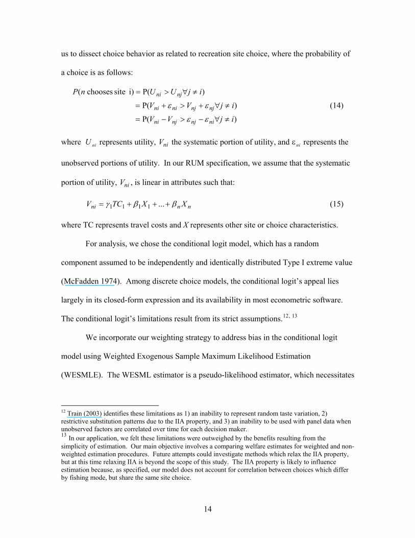
us to dissect choice behavior as related to recreation site choice, where the probability of

a choice is as follows:

)P(

)P(

)P(i) site chooses(

ijVV

ijVV

ijUUnP

ninjnjni

njnjnini

njni

≠∀−>−=

≠∀+>+=

≠∀>=

εε

εε (14)

where U represents utility, the systematic portion of utility, and ε represents the

unobserved portions of utility. In our RUM specification, we assume that the systematic

portion of utility, , is linear in attributes such that:

ni niV ni

niV

nnni XXTCV ββγ +++= ...1111 (15)

where TC represents travel costs and X represents other site or choice characteristics.

For analysis, we chose the conditional logit model, which has a random

component assumed to be independently and identically distributed Type I extreme value

(McFadden 1974). Among discrete choice models, the conditional logit’s appeal lies

largely in its closed-form expression and its availability in most econometric software.

The conditional logit’s limitations result from its strict assumptions.12, 13

We incorporate our weighting strategy to address bias in the conditional logit

model using Weighted Exogenous Sample Maximum Likelihood Estimation

(WESMLE). The WESML estimator is a pseudo-likelihood estimator, which necessitates

12 Train (2003) identifies these limitations as 1) an inability to represent random taste variation, 2) restrictive substitution patterns due to the IIA property, and 3) an inability to be used with panel data when unobserved factors are correlated over time for each decision maker. 13 In our application, we felt these limitations were outweighed by the benefits resulting from the simplicity of estimation. Our main objective involves a comparing welfare estimates for weighted and non-weighted estimation procedures. Future attempts could investigate methods which relax the IIA property, but at this time relaxing IIA is beyond the scope of this study. The IIA property is likely to influence estimation because, as specified, our model does not account for correlation between choices which differ by fishing mode, but share the same site choice.

14

a robust sandwich estimator to calculate the variance-covariance matrix. The corrected

asymptotic covariance structure is:

11 −− ΔΩΩ=V (16)

where

.'

),,(log),(),,(log),(

'),,(log),(

**

*

2

⎥⎥⎦

⎤

⎢⎢⎣

⎡⎟⎟⎠

⎞⎜⎜⎝

⎛∂

∂⎟⎟⎠

⎞⎜⎜⎝

⎛∂

∂=Δ

⎥⎥⎦

⎤

⎢⎢⎣

⎡⎟⎟⎠

⎞⎜⎜⎝

⎛∂∂

∂−=Ω

ββ

β

ββ

ββ

βββ

ziPziwziPziwE

ziPziwE

nnnn

nn

Without this correction, the standard errors are biased downwards.

We compare welfare estimates for our weighting procedures by evaluating the

impact of an increase in catch by one fish. We evaluate this welfare impact using the

following formula

( ) ( )[ ]γ

βγβγ

−

−=Δ ∑∑ ++ *lnln

)(xTCxTC ee

CatchWTP (17)

where βγ xTC + represents the indirect utility of a given choice without a change,

βγ xTC + represents the indirect utility after the change, and γ represents the travel cost

parameter. We first calculate the WTP for a one fish increase in catch rate and then

calculate confidence intervals to compare the accuracy of our weights. We take 1500

random draws of the model coefficients from an asymptotic multivariate normal

distribution of the parameter estimates using the Krinsky-Robb procedure (Krinsky and

Robb, 1986). We then determine confidence intervals for the WTP for each historic

catch measure. These measures are developed to compare the distribution of WTP within

species groupings.

15

Data

In this paper, our primary interest lies in determining the effectiveness of

propensity score based weights which address onsite sample selection biases. First, we

create a dataset which simulates the onsite sampling process. This allows us to compare

estimates of various weighting schemes using the simulated onsite sample to a model

estimated using the true population dataset. We follow this simulation with an empirical

application that focuses on the recreation site choice of anglers living in coastal counties

in the southeastern and Gulf regions of U.S.

Our simulated and empirical applications utilize data from the National Marine

Fisheries Service’s Marine Recreational Fishery Statistics Survey (MRFSS). Since 1994,

NMFS has used the Marine Recreational Fishing Statistics Survey (MRFSS) as its

primary vehicle for revealed preference studies. In addition to information on

recreational fish catch, the MRFSS has been used to gather the travel cost data necessary

to estimate the values of access and changes in catch rates.

The MRFSS, which is designed to estimate recreational fishing catch and effort,

has two primary components, an intercept survey and a RDD telephone survey. The

MRFSS also includes an economic add-on. The simulation and empirical portions of this

study investigate the implications of intercept based sampling procedures in the

estimation of discrete choice models of recreation site choice. Our simulation treats the

intercept data as if it were the true angler population. We then take a sample from the

intercept data by simulating a stratified onsite sampling process. The empirical portion of

this study uses both the intercept and RDD data. The MRFSS employs a choice-based

16

sample (i.e. endogenously stratified) of intercept sites; however, sampling intensity is

proportional to the fishing pressure at each site.

The southeastern and Gulf states sampled by the MRFSS include North Carolina,

South Carolina, Georgia, Florida, Alabama, Mississippi, and Louisiana. The MRFSS

data were stratified by state, fishing mode (private/rental, party/charter, shore), and 2

month wave. Sampling was conducted between the beginning of September 2003 and the

end of August 2004. We limit observations to those anglers fishing by private and rental

boat who were on single day trips. Multiple day trips were eliminated because these

anglers may also be participating in multi-purpose trips and may exhibit different

preferences and single-trip takers.

Because we assume each fisherman in the sample takes a single day trip, we also

chose to limit all angler choice sets using geographic bounds. Our model eliminates all

site choices beyond a 200 mile one way distance. Parsons and Hauber (1998) show that

choice sets can be limited by the number of choices, using distance as an inclusion

threshold. Whitehead and Haab (2000) apply this method to the MRFSS, finding that

limiting choice sets to all sites within 180 miles has minimal impact on welfare estimates.

In our empirical application, we further truncate the intercept survey to meet the

classification of a coastal county population, as sampled in the RDD survey. The

truncation of the intercept sample shrinks the angler population to those anglers residing

in coastal counties who targeted specific species types.14 These forms of sample

truncation were performed for the convenience of comparison and, as a result, we do not

expect our empirical results to represent the larger population of saltwater anglers.

14 An indirect consequence of only including individuals who targeted specific species seems to have led to more avid users within both samples.

17

Because our efforts focus on the role weighting strategies play on correcting non-random

sample selection biases, we felt the need to minimize geographic and non-sampling

related behavioral differences. As such, future studies should focus on obtaining

estimates which cover a more complete portion of the saltwater recreational angler

population. Our simulated datasets are not limited to the coastal county population, but,

as discussed earlier, they are limited by distance. As a result there are differences

between the intercept data used in the simulation exercise and the intercept data used in

the empirical application.

In regional recreation demand models, it is often necessary to aggregate

characteristics of the choice occasion because of limitations in coverage across the data

set. County level site aggregations are necessary due to a lack of RDD data for smaller

geographic scales of site visitation. These site aggregations lead to 67 coastal counties in

the choice set. We also assume recreational anglers target fish among four different

species groupings (Off-Shore Species, In-Shore Species, Reef Species, and Pelagic

Species). These species groupings account for the majority of fish species targeted by

recreational users in the Southeastern and Gulf regions.15 We represent fishing quality at

each site by the 5-year average historical catch (both kept & released fish) for each site.

This proxy measure represents fishing stock quality at each site, specific to the particular

fishing mode. A rationally consistent angler should seek out sites they perceive allow

access to higher quality stocks.16

15 Off-Shore species include individual species such as Amberjack, King Mackerel, and Spanish Mackerel. In-Shore species account for species such as various types of Flounder, Tarpon, Croaker, and Red Drum. Reef species includes Grouper, Red Snapper, Black Seabass, and others. Pelagic species include various species such as Tuna, Wahoo, and Swordfish. 16 We also assume that anglers use information on released fish at a site to estimate site quality in addition to kept fish. Also, some fish, such as Tarpon, are largely catch and release species. Without information on released fish, these species would not be adequately represented in the model.

18

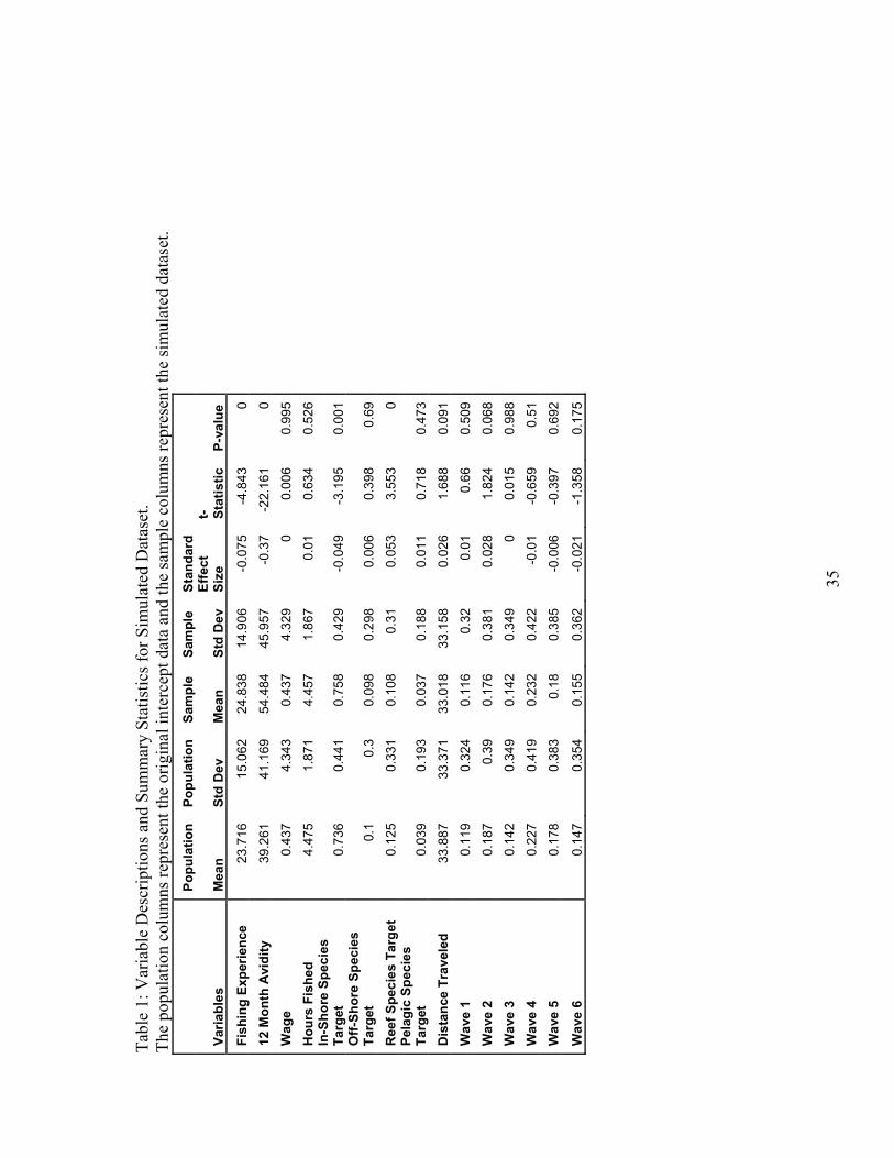
Table 1 provides unweighted descriptive statistics for relevant variables from the

intercept and simulated datasets. For the simulation, we treat the intercept data as the

true population and perform our onsite sampling process using the sample command,

which is a base function within the statistical software system R (R Core Development

Team 2009). In our sampling process, we first stratify the intercept sample by site and

then choose anglers, without replacement, from each site according to fishing pressure at

the site. We make sure to oversample less frequented sites and under-sample more

frequented sites, thus guaranteeing an endogenously stratified sample.17 Within each

strata or site, the random selection of anglers was altered through the use of a vector of

probability weights. The probability weights were calculated by taking the number of

trips taken by an individual angler in the previous year divided by the total number of

days in the year. This weight guarantees a size-biased sampling process.

Table 1 also includes test statistics for t-tests of significance of the differences in

the variable means,18and the standardized effect sizes, which are the difference between

the treatment group mean values and the control group mean values divided by the

treatment group standard deviation. Cohen (1988) states that, when using the

standardized effect size, a rule of thumb generally applies where values up to 0.2

represent small differences in means, values around 0.5 represents medium sized

differences, and values over 0.8 represent large differences.19

17 The MRFSS intercept survey also samples according to fishing pressure. When estimates of fishing pressure match fishing pressure in the general population, this can address endogenous stratification in the discrete choice setting. Endogenous stratification can occur, however, when estimates deviate from the true fishing pressure. 18 When we evaluate the t statistics testing differences in means for all available variables, which include variables in table 1 as well as site specific constants, we find that 33 means are statistically different than zero at the .1 significance level. 19 Using Cohen’s rule of thumb only one variable, 12 month avidity, classifies as a medium sized absolute difference. All other variables represent small absolute differences.

19

Our intercept data set accounts for usable data from anglers that were first

intercepted at fishing sites and then agreed to participate in the Add-On MRFSS

Economic Survey (AMES). The AMES survey collects additional economic information,

such as travel costs and expenditures. In the simulation exercise, our intercept sample

uses 11,821 surveys of anglers in the Southeast and Gulf regions. Of the anglers in this

sample, 73 % targeted inshore species, 10% targeted offshore species, 13% targeted reef

species, and 4% targeted pelagic species. The average intercepted angler has fished for

23.71 years and fished 39 times in the 12 previous months. They traveled 34 miles on

average and fished for 4.48 hours.

In our simulated sample of 6429 anglers, 76% targeted inshore species, 10%

targeted offshore species, 11% targeted reef species, and 4% targeted pelagic species.

The average angler in this dataset has fished for 24.84 years and has fished 54.48 times in

the last year (evidence of avidity bias when compared to the “population” estimate of 39).

On their latest trip, the average angler traveled 33 miles and fished for 4.46 hours.

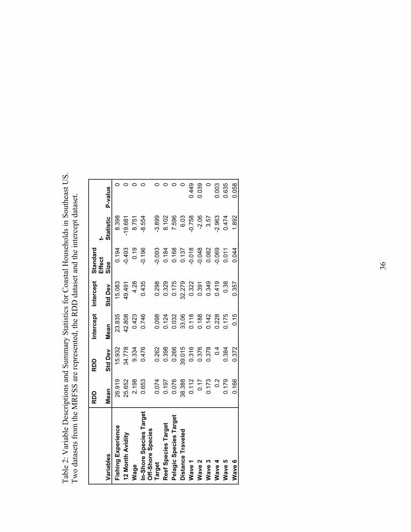
Table 2 provides the descriptive statistics for coastal households in the intercept

and RDD samples.20 We utilize 11,618 anglers from the intercept survey and 2202

anglers from the RDD survey. The average angler in the intercept survey has fished for

24 years and fished 43 times in the previous year. Of these anglers, 75% targeted inshore

species, 10% targeted offshore species, 12% targeted reef species, and 3% targeted

pelagic species. The average angler in this sample traveled 38 miles to their fishing site.

In the RDD sample, roughly 65% targeted inshore species, 7 % targeted offshore species,

20% targeted reef species, and 8% targeted pelagic species. The average angler in the

20 When we evaluate differences between the intercept and RDD surveys, 50 differences in means are statistically different than zero and three variables have medium sized absolute differences.

20

RDD sample has fished for almost 27 years and fished roughly 26 times in the 12 months

before being interviewed. They also traveled 38 miles on average.

It is important to note that there are several differences in the scale of information

between the MRFSS intercept and RDD samples. The RDD survey collects information

on the county in which an angler fishes, but does not collect information on the specific

site. In this way, the intercept distance estimates are more representative of the true

distance traveled by an angler, since the RDD only reveals distances to the center of the

county. Also, individuals in the RDD sample may fish from sites not covered by the

intercept sampling process. These factors likely diminish the level of precision of an

estimated weight within the choice model.

Results

Each of our analyses has two steps. First, we calculate the propensity score based

weight and then we utilize this weight during the estimation of the recreation site choice

models. The first analysis makes use of simulated data (using the intercept sample as the

true population) and the second is an empirical application using MRFSS intercept and

RDD data.

Using simulated data, we compare four different estimation procedures so to

illustrate the effect of onsite sample selection biases on estimation. The estimation

procedures differ according to assumptions defining the data generation process. The

first estimation procedure does not correct for endogenous stratification or size-biased

sampling. The unweighted estimator assumes the intercept data is collected at random.

The second estimation procedure utilizes a variation of Cosslett’s (1981) weight within

21

WESMLE. This second procedure, which we will call the basic WESMLE, assumes that

the sample is a pure choice-based sample, meaning the data generating process within

each sample strata occurs at random. We estimate the basic WESMLE using a logistic

regression with site specific constants to generate the weights.21 The third procedure,

which we refer to as avidity-only WESMLE, only addresses avidity bias. The weights

are produced using a propensity score in which 12 month avidity is the only covariate.

This approach assumes that all sampling bias results from the size biased sampling

process (i.e. avidity bias) and no endogenous stratification exists. The fourth and last

weight, which we call the balanced WESMLE, does not assume random selection within

strata, but rather accounts for both endogenous stratification and avidity bias. This

procedure utilizes the propensity-score weight, which is estimated using GBM

(Ridgeway 2007a).22

In the calculation of both the basic- and balanced-WESMLE weights, the

propensity score based weight is an odds ratio, where the numerator of this ratio

represents the probability of inclusion in the simulated sample conditional on relevant

covariates and the denominator represents the probability of inclusion in the auxiliary

dataset conditional on relevant covariates. The estimation of the propensity score based

weights for the balanced WESMLE requires some type of variable selection process for

determining the proper model specification. Beyond differences resulting from sampling

21 We found that when the odds ratio of this propensity score estimator is standardized by dividing it by its mean value, it is equivalent to the Cosslett estimator (i.e. estimated population shares divided by sample shares). 22 While the GBM function does adaptively fit a model, an analyst is required to choose the relevant variables as well as the number of potential variable interactions and the size of a step in a given iteration. We include all available variables (site, wave, fish targeted, avidity, years fished, distance traveled, and hours fished (if available),) in the model. We allow for up to 4 variable interactions and choose a step size of 0.0005. The small step size can improve precision, but necessitates a higher number of iterations during estimation.

22

intensity between strata and size-biased sampling, there are no theories to drive the

choice of covariates in the weight. GBM uses an algorithm which adaptively selects

variables according to improvements in the log likelihood. Following estimation, we use

the odds ratio, as seen in equation (9), to “quasi-randomize” the intercept data.

Next, we need a method to evaluate the effectiveness of each weight. We

evaluate these weights using two graphical depictions of balance. The first depiction of

balance plots the p-values from t-tests, which compare the variable means in the control

and treatment groups. This graph also includes a 45-degree line, which represents a

uniform cumulative distribution. When p-values are larger than the points on this line,

we can conclude that the differences in means are at least as small as what would be

expected in a randomized study (Ridgeway 2006). Each graph plots both weighted and

unweighted p-values. These graphs for the three weights can be found in figure 1. Using

this graphical depiction of balance, we see that the basic WESMLE weight (graph 1a.)

and the balanced WESMLE weight (graph 1c) appear to improve the balance of most

variables and also outperform the avidity-only WESMLE (graph 1b).

Figure 2 shows the second graph for balance assessment, which Ridgeway (2006)

calls the effect size plot. This graph depicts the effect of the weighting procedure on the

magnitude of differences in variables between the treatment and control groups. More

successful balancing procedures should decrease the magnitude of differences. In this

graph, the magnitude of differences for the unweighted procedure can be found on the

left hand side. This magnitude is compared to the weighted results, which are plotted on

the right hand side. For each variable, a line connects the weighted and unweighted

procedure. When the weighting procedure decreases (increases) the magnitude of the

23

difference between the means, the line has a negative (positive) slope. We see in Figure

2 that the balanced WESMLE weight (graph 2c) performs best, followed by the basic

WESMLE weight (graph 2a). According to this graph, the avidity-only WESMLE

appears to perform the worst (graph 2b).

In our analysis of angler choice between site and fishing mode, we model choice

as a function of travel cost, travel time, the log transformation of the number of intercept

sites in the county aggregation, and fishing quality measures represented by 5 year mean

historic catch rates. For each aggregated historic catch rate, we include the value as well

as the squared value so to capture non-linear responses to catch.

Travel costs are calculated as a combination of the explicit costs of travel and the

anglers’ opportunity costs of time. We estimate the explicit cost of travel as the round

trip distance times 35 cents per mile.23 If anglers lost income by taking the trip, their

opportunity cost of time was estimated as their wage rate multiplied by the average travel

time, which was round trip distance divided by their average speed (40 mph).24 When

anglers did not lose income by taking the trip, we set their opportunity cost of time to

zero. For these anglers, we capture their opportunity cost of time with a separate

measure, travel time. The travel time variable is set to zero for anglers who lost income

and is equal to the travel distance divided by average travel speed (40 mph) for all other

anglers.

We control for site aggregation bias using the natural log transformation for the

number of intercept sites within each county aggregation. In RUMs, site aggregation can

lead to biased coefficient estimates (Haener, Boxall, Adamowicz, and Kuhnke 2004).

23 Travel distances are calculated using the software package PCMiler. 24 We assume that the average travel speed is 40 mph. This measure was previously used with the MRFSS by Hicks et al. (1994).

24

Haener, Boxall, Adamowicz, and Kuhnke recommend including the log transformation of

the site area to capture the size of aggregation. They found that when recreation demand

models of site choice account for the size of aggregates during estimation, model

parameters can be equivalent across scales. It should be noted, however, that our site

aggregations do limit our ability to capture site specific characteristics that would be

captured with finer scale site definitions. These aggregations were the product of the

overall sampling strategy.

Table 3 provides the estimation results for all our models. As expected, the travel

cost measure has a negative sign, indicating the inverse relationship between the

opportunity costs of travel and site choice. The results also show a nonlinear, positive

relationship between the 5-year historic catch rates and the probability of choice. This

coincides with the assumption that anglers seek out sites with higher quality fishing

stocks. In the simulated samples, inclusion of the weight leads to statistically

insignificant coefficients on both offshore catch and squared offshore catch.

Next we compare welfare estimates for our weighting procedures. In each model,

we evaluate the impact of an increase in catch by one fish. These measures are

developed to compare the distribution of WTP within species groupings. Table 4 gives

the results of the WTP point estimates as well as the 95% confidence intervals derived

via the Krinsky-Robb procedure.

Our first welfare measure for comparison represents the 5 year historic catch rate

for inshore species. For the simulated data, when we compare the estimates from our

population to the unweighted and weighted procedures, the basic WESMLE weight

performs best, with a difference in point estimates of 13%. The point estimate for the

25

balanced WESMLE differs from the population measure by 15%. It is interesting that the

Avidity weight actually performs worse (35% difference), than the unweighted model

(19% difference). Figure 3a depicts boxplots of the 95% confidence intervals for this

procedure. We find significant overlap between the different procedures. When we

evaluate the influence of the balanced WESMLE procedure on an increase in inshore

species catch, we find the WTP point estimate decreases by 31%.

When we evaluate WTP for a one fish increase in offshore catch rates, we find

that the only estimation procedures with statistically significant WTP measures are the

results from the population estimator and the avidity weighted estimator for the simulated

datasets. When we evaluate point estimates only, we find the avidity weighted WTP

measure to be 88% greater than the population measure. Figure 3b illustrates the

confidence distribution of the WTP for the different simulated dataset estimators.

Next we compare WTP for an increase in reef species catch rates. In the

simulated dataset, we find the balanced WESMLE performs best with a 12% difference

in point estimates. The basic WESMLE performs second best with a difference of 20%.

The unweighted estimator has a WTP value greater by 48% and the avidity weight has a

WTP value greater by 34%. Figure 3c depicts boxplots of the 95% confidence intervals

for the WTP measures.

Our last comparison utilizes estimates for WTP for pelagic species. Here, the

balanced WESMLE estimator performs much better than the other estimators with a

difference of 43% in the point estimate. The basic WESMLE estimator performs second

best with a difference of 80%. The avidity estimator performs the worst with a difference

26

of 198% and the unweighted estimator has a WTP point estimate 98% greater than the

population dataset. Figure 3d depicts the 95% confidence intervals for WTP.

When we evaluate the overall effectiveness of the various weighting strategies

using the point estimates of WTP, we find that, on average, the balanced WESMLE

performs best with an average difference in WTP of 26%. The second best performing

weight is the basic WESMLE estimator with an average difference in WTP of 39%. The

avidity weight actually performs worse than the unweighted estimator with an average

difference of 89% versus 45% for the unweighted estimator.

We follow our analysis of the simulated data with an empirical application. In

our empirical application, we estimate weights using the RDD sample of coastal

households. Our primary objective involves a comparison of the balanced WESMLE

procedure and the unweighted estimator since the balanced WESMLE outperformed the

other weighting strategies in our simulated exercise. First, we need to evaluate the

performance of the balancing procedure. Figure 4a depicts a graph evaluating the

differences in means for the intercept and RDD samples using the propensity score based

weight. Much like the simulated exercise, we find improvement in the differences in

means between the unweighted and weighted. Figure 4b, which depicts the effect size

plot for the RDD and intercept samples, shows that the propensity score based weight

also reduces the effect size.

Next, we estimate the recreation site choice model with the identical model

specification as used in our simulated exercise. Results for the empirical models can be

found in table 3. Much like the simulated example, inclusion of the weight leads to

statistically insignificant coefficients on both offshore catch and squared offshore catch.

27

The balanced WESMLE also leads to insignificant coefficients on both pelagic and

squared pelagic catch.

Willingness-to-pay point estimates and confidence intervals can be found in table

4. As we found in the simulated exercise, the unweighted estimators appear to suffer

from upward bias in the WTP measures for one additional caught fish. We find that the

weighting strategy leads to a 31% decrease in the WTP for an additional inshore species

and a 6% decrease in the WTP for an additional reef species. We do not find statistically

significant WTP measures for changes in catch of offshore or pelagic species. Figures

5a-5c shows boxplots of the 95% confidence intervals for WTP from the unweighted and

weighted procedures using the RDD weighted dataset.

Discussion & Conclusions

In November of 2006, the Center for Independent Experts (CIE), located in the

Rosenstiel School of Marine and Atmospheric Science at University of Miami, solicited a

review of recreational economic data at the NMFS. The review addressed key questions

dealing with the economic data used in the estimation of revealed preference models,

conjoint analysis, and economic impact analysis (CIE 2006). As one topic addressed by

the CIE, the review discusses the implications of onsite sampling procedures in the

estimation of discrete choice models of recreational site choice. In addition to the

potential bias resulting from endogenous stratified sampling (i.e. stratified by choice),

past studies have indicated that the MRFSS data is also prone to size-biased sampling,

specifically in the form of avidity bias (Thompson 1991).

28

Onsite samples provide a cost effective method of eliciting recreational users’

preferences. For the National Marine Fisheries Service (NMFS), a separate revealed

preference survey would cost more than two times the current costs of the MRFSS

economic add-on (CIE 2006). This dramatic difference in cost highlights the value of

estimation procedures which allow for the utilization of existing data sources. While the

primary purpose of the MRFSS is to estimate fishing catch and effort for recreational

anglers, the data brings additional value when utilized for economic analysis.

Conducting RP studies using data collected from the MRFSS allows the NMFS to extend

resources to other areas of need, including valuation via stated preference methods.

The CIE report identifies onsite sampling as one of the primary sources of bias in

estimating revealed preference studies that use the MRFSS. If the sampling process leads

to differences in the sampling intensity of site choices between the sample and the true

population, this bias occurs in the form of both endogenous stratification and size-biased

sampling. If the MRFSS sampling procedure, which does account for fishing pressure at

intercept sites, does not lead to differences in sampling intensity of site choices, then the

relevant bias occurs in the form of size-biased sampling. We propose utilizing propensity

score based weights to address relevant biases. In our empirical application, we develop

this weight using auxiliary data from a RDD survey of coastal anglers.

Past recreation demand studies have addressed truncation and avidity in single

site recreational demand models. Unlike the single site recreation demand literature,

there have been few studies of recreation site choice which address bias from onsite

sampling. Moeltner and Shonkwiler (2005) utilize panel data to address onsite sampling

for repeated recreation site choices. Moeltner and Shonkwiler sample individual trips,

29

but also collect information on all other trips taken within a system of sites. In their

study, they adopt a Dirichlet-multinomial distribution rather than a multinomial

distribution, which allows them to also address overdispersion in the sample. A

dispersion parameter picks up variability in trip counts, which allows them to control for

size-biased sampling. Their model also accounts for onsite sampling biases by adjusting

the likelihood function for observed trips divided by expected trip counts for the sampled

sites. To our knowledge, there are no studies of recreation site choice that address both

avidity bias and endogenous stratification for single choice occasions in a multinomial

setting.

Our results indicate that failure to account for differences in angler attributes can

lead to significant upward bias in the point estimates of welfare measures. This result

coincides with the well documented effect of avidity bias within other types of recreation

demand models. Utilizing our simulated dataset with an unweighted estimator, on

average, we find point estimates of WTP for changes in fishing catch to be biased upward

by 45%. When we only account for endogenous stratification, the point estimates for

WTP are still biased upward by 39% on average. In the presence of both endogenous

stratification and size-biased sampling, the avidity weight, which only accounts for size-

biased sampling, actually increases the bias in point estimates to an average of 89%.

Our proposed method, the balanced WESMLE accounts for both size-biased

sampling and endogenous stratification. This weight proves to outperform the other

weighting strategies for addressing bias in WTP point estimates. We find significantly

less bias in these WTP point estimates when compared to the other weighting strategies –

upward bias is reduced to roughly 26% on average. These results indicate that, when

30

using onsite samples with both endogenous stratification and size-biased sampling,

analysts must account for differences in characteristics of the recreational user in addition

to differences in sampling intensity. Importantly, in the presence of both endogenous and

size-biased sampling, the weight which only accounts for avidity bias consistently

performs worse than the unweighted estimator.

Our propensity score based weights offer a viable option for correcting bias due to

onsite sampling. One limiting factor involves finding adequate data to qualify as

auxiliary data. In our empirical application, the RDD survey of coastal households may

address some of the relevant biases associated with onsite sampling, but differences in the

scale of measurement likely limits the accuracy of these weights. The RDD survey also

fails to account for anglers who reside outside coastal regions. As states begin to

implement licensing requirements for recreational anglers, management agencies can

periodically collect samples of anglers for weighting purposes. These surveys could also

be used to fine tune the sampling intensity at various intercept sites. Researchers may

also wish to utilize a mixed sampling strategy where they collect an initial RDD sample

followed by a lower cost onsite sampling strategy. The RDD sample could be first used

to gauge the intensity of site choice for onsite sampling and later reweighting to account

for other exogenous/endogenous differences in sample selection.

It should be noted that, while our weights improve the consistency of RUM

estimates, our simplified specification has only limited policy applications. Fishery

management decisions are more likely to focus on individual species, rather than species

aggregations. Unfortunately, the MRFSS does not have adequate coverage to address

every key species on a regional basis. A future extension to this research would apply

31

this method to individual species. Up to this point, the NMFS has addressed some of

these limitations which result from these coverage and flexibility issues with stated

choice experiments. In addition to the limitations associated with species and site

aggregations, our empirical example is also limited to households in coastal counties.

Among the numerous potential differences between anglers in coastal counties and the

larger population, these coastal households are likely to be more avid users. As a result,

our sample is not representative of the larger saltwater angler population.

Last, our method results in consistent estimates when using a conditional logit

model, but does not lead to consistent results in other types of discrete choice models

such as nested logit models, cross-nested logit models, and mixed logit models (Bierlaire,

Bolduc, and McFadden 2008). Future studies should investigate methods which can

address non-random sample selection bias while relaxing the IIA property as well as

incorporating preference heterogeneity.

References

Bierlaire, M., D. Bolduc, and D. McFadden. 2008. “The estimation of Generalized Extreme Value models from choice-based samples.” Transportation Research: Part B. 42: 381-394.

Breiman, L., J.H. Friedman, R.A. Olshen, and C.J. Stone. 1984. Classification and Regression Trees Belmont, CA: Wadsworth International Group.

Center for Independent Experts. 27 November 2006 Review of Recreational Economic Data at the National Marine Fisheries Service. Kenneth McConnell (chair).

Cohen, J. 1988. Statistical Power Analysis for the Behavioral Sciences. Academic Press, New York, 2nd ed.

Cosslett, S. 1981. “Maximum Likelihood Estimator for Choice-based Samples.” Econometrica. 49(5): 1289-1316.

Dehejia, R. and S. Wahba. 2002. “Propensity Score Matching Methods for Nonexperimental Causal Studies.” Review of Economics and Statistics. 84(1): 151-161.

Englin, J. and J. Shonkwiler. 1995. “Estimating Social Welfare using Count Data Models: An Application to Long-run Recreation Demand under Conditions of

32

Endogenous Stratification and Truncation.” The Review of Economics and Statistics. 77: 104-112.

Friedman, J.H. 2001. “Greedy Function Approximation: A Gradient Boosting Machine.” Annals of Statistics. 29: 1189-1232.

Friedman, J.H. 2002. “Stochastic Gradient Boosting.” Computational Statistics and Data Analysis. 38: 367-378.

Friedman, J.H., T. Hastie, and R. Tibshirani. 2000. “Additive logistic regression: A statistical view of boosting.” Annals of Statistics. 28: 337-374.

Haab, T. and K. McConnell. 2003. Valuing Environmental and Natural Resources: The Econometrics of Non-Market Valuation. Edward Elgar: Northampton, MA.

Haener, M.K., P.C. Boxall, W.L. Adamowicz, and D.H. Kuhnke. 2004. “Aggregation Bias in Recreation Site Choice Models: Resolving the Resolution Problem.” Land Economics. 80(4): 561-574.

Hastie, T., R. Tibshirani, and J.H. Friedman. 2001. The Elements of Statistical Learning. New York: Springer-Verlag.

Heckman, J.J. and S. Navarro. 2004. “Using matching, instrumental variables, and control functions to estimate economic choice models.” Review of Economics and Statistics. 86(1): 30-57.

Hirano, K. and G. Imbens. 2001. “Estimation of causal effects using propensity score weighting: An application to data on right heart catheterization.” Health Services and Outcomes Research Methodology. 2: 259-278.

Hirano, K, G. Imbens, and G. Ridder. 2003. “Efficient estimation of average treatment effects using the estimated propensity score.” Econometrica. 71: 1161-1189.

Hsieh D.A., C. Manski, and D. McFadden. 1985. “Estimation of Response Probabilities From Augmented Retrospective Observations.” Journal of the American Statistical Association. 80(391): 651-662.

Krinsky, I, and A.L. Robb. 1986. “On approximating the statistical properties of elasticities.” Review of Economics and Statistics. 68: 715-719

Little R. and D. Rubin. 1987. Statistical Analysis with Missing Data. New York: Wiley. Manski, C. and S. Lerman (1977), ‘The Estimation of Choice Probabilities from Choice

Based Samples’, Econometrica 45, 1977–1988. Manski C.F. and D. McFadden. 1981. “Alternative Estimators and Sample Designs for

Discrete Choice Analysis.” .” In Structural Analysis of Discrete Data, C.R. Manski and D. McFadden (eds) Cambridge, Massachusetts: MIT Press. 1981.

McCaffrey, D., G. Ridgeway, and A. Morral 2004. “Propensity score estimation with boosted regression for evaluating adolescent substance abuse treatment.” Psychological Methods. 9(4): 403-425.

McFadden, D. (1974), ‘Conditional Logit Analysis of Qualitative Choice Behavior’ in P. Zarembka, ed., Frontiers of Econometrics. Academic Press.

McFadden, D. 1999. Econometrics 240B Reader. Unpublished manuscript. UC Berkeley.

Moeltner, K. and J.S. Shonkwiler. 2005. “Correcting for On-Site Sampling in Random Utility Models.” American Journal of Agricultural Economics. 87(2): 327-339.

National Research Council (NRC). 2006. Review of Recreational Fisheries Survey Methods. National Academies Press, Washington, D.C.

33

34

Nevo, A. 2003. “Using weights to adjust for sample selection when auxiliary information is available.” Journal of Business and Economics Statistics. 21(1): 43-52.

Parsons, G. and B. Hauber. 1998. “Spatial Boundaries and Choice Set Definition in a Random Utility Model of Recreation Demand.” Land Economics. 74(1): 32-48.

Patil, G.P. and C.R. Rao. 1978. “Weighted Distributions and Size-Biased Sampling with Applications to Wildlife Populations and Human Families.” Biometrics. 34: 179-189.

R Development Core Team. 2009. R: A Language and Environment for Statistical Computing. R Foundation for Statistical Computing, Vienna, Austria. ISBN 3-900051-07-0. http://R-project.org.

Ridgeway, G. 2006. “Assessing the effect of race bias in post-traffic stop outcomes using propensity scores.” Journal of Quantitative Criminology. 22(1): 1-29.

Ridgeway, G. 2007a. “Generalized Boosted Models: A guide to the gbm package.” http://cran.r-project.org/src/contrib/Descriptions/gbm.html

Ridgeway, G. 2007b. gbm: Generalized booseted Regression models Version 1.6-3. http://cran.r-project.org/doc/vignettes/gbm/gbm.pdf

Ridgeway, G., D McCaffrey, and A. Morral. 2006. twang: Toolkit for Weighting and Analysis of Nonequivalent Groups Version 1.0-1. http://cran.r-project.org/src/contrib/Descriptions/twang.html

Ridgeway, G., D McCaffrey, and A. Morral. 2006. “Toolkit for Weighting and Analysis of Nonequivalent Groups: A tutorial for the twang package.” http://cran.r-project.org/bin/windows/contrib/r-release/twang_1.0-1.zip

Rosenbaum, P. and D.B. Rubin. 1983. “The central role of the propensity score in observational studies for causal effects. Biometrika. 70: 41-55.

Sargeant, F. 2010. “Anglers head to Washington to voice concerns.” Tampa Bay Online. Link: http://www2.tbo.com/content/2010/feb/21/sp-march-madness/sports-outdoors/

Shaw, D. 1988. “On-Site Samples’ Regression: Problems of Non-negative Integers, Truncation, and Endogenous Stratification.” Journal of Econometrics. 37: 211-223.

Train, K. (2003), Discrete Choice Methods with Simulation. Cambridge, UK: Cambridge University Press.

Thompson, C. 1991. “Effects of Avidity Bias on Survey Estimates of Fishing Effort an Economic Value, in Creel and Angler Surveys in Fisheries Management. American Fisheries Society Symposium. 12: 356-66.

Whitehead, J. C., and T. C. Haab. 2000. “Southeast Marine Recreational Fishery Statistical Survey: Distance and Catch Based Choice Sets.” Marine Resource Economics. 14: 283-298.

Wooldridge, J. 2002. “Inverse probability weighted M-estimators for sample selection, attrition, and stratification.” Portuguese Economic Journal. 1: 117-139.

Tabl

e 1:

Var

iabl

e D

escr

iptio

ns a

nd S

umm

ary

Stat

istic

s for

Sim

ulat

ed D

atas

et.

Th

e po

pula

tion

colu

mns

repr

esen

t the

orig

inal

inte

rcep

t dat

a an

d th

e sa

mpl

e co

lum

ns re

pres

ent t

he si

mul

ated

dat

aset

.

Po

pula

tion

Popu

latio

n Sa

mpl

e Sa

mpl

e St

anda

rd

Varia

bles

M

ean

Std

Dev

M

ean

Std

Dev

Ef

fect

Si

ze

t- Stat

istic

P-

valu

e

Fish

ing

Expe

rienc

e 23

.716

15

.062

24

.838

14

.906

-0

.075

-4

.843

0

12 M

onth

Avi

dity

39

.261

41

.169

54

.484

45

.957

-0

.37

-22.

161

0

Wag

e 0.

437

4.34

3 0.

437

4.32

9 0

0.00

6 0.

995

Hou

rs F

ishe

d 4.

475

1.87

1 4.

457

1.86

7 0.

01

0.63

4 0.

526

In-S

hore

Spe

cies

Ta

rget

0.

736

0.44

1 0.

758

0.42

9 -0

.049

-3

.195

0.

001

Off-

Shor

e Sp

ecie

s Ta

rget

0.

1 0.

3 0.

098

0.29

8 0.

006

0.39

8 0.

69

Ree

f Spe

cies

Tar

get

0.12

5 0.

331

0.10

8 0.

31

0.05

3 3.

553

0Pe

lagi

c Sp

ecie

s Ta

rget

0.

039

0.19

3 0.

037

0.18

8 0.

011

0.71

8 0.

473

Dis

tanc

e Tr

avel

ed

33.8

87

33.3

71

33.0

18

33.1

58

0.02

6 1.

688

0.09

1

Wav

e 1

0.11

9 0.

324

0.11

6 0.

32

0.01

0.

66

0.50

9

Wav

e 2

0.18

7 0.

39

0.17

6 0.

381

0.02

8 1.

824

0.06

8

Wav

e 3

0.14

2 0.

349

0.14

2 0.

349

0 0.

015

0.98

8

Wav

e 4

0.22

7 0.

419

0.23

2 0.

422

-0.0

1 -0

.659

0.

51

Wav

e 5

0.17

8 0.

383

0.18

0.

385

-0.0

06

-0.3

97

0.69

2

Wav

e 6

0.14

7 0.

354

0.15

5 0.

362

-0.0

21

-1.3

58

0.17

5

35

Tabl

e 2:

Var

iabl

e D

escr

iptio

ns a

nd S

umm

ary

Stat

istic

s for

Coa

stal

Hou

seho

lds i

n So

uthe

ast U

S.

Two

data

sets

from

the

MR

FSS

are

repr

esen

ted,

the

RD

D d

atas

et a

nd th

e in

terc

ept d

atas

et.

RD

D

RD

D

Inte

rcep

t In

terc

ept

Stan

dard

Varia

bles

M

ean

Std

Dev

M

ean

Std

Dev

Ef

fect

Si

ze

t- Stat

istic

P-

valu

e Fi

shin

g Ex

perie

nce

26.9

19

15.9

32

23.8

35

15.0

83

0.19

4 8.

398

012

Mon

th A

vidi

ty

25.6

52

34.7

78

42.8

08

49.4

91

-0.4

93

-19.

681

0W

age

2.19

8 9.

334

0.42

3 4.

28

0.19

8.

751

0In

-Sho

re S

peci

es T

arge

t 0.

653

0.47

6 0.

746

0.43

5 -0

.196

-8

.554

0

Off-

Shor

e Sp

ecie

s Ta

rget

0.

074

0.26

2 0.

098

0.29

8 -0

.093

-3

.899

0

Ree

f Spe

cies

Tar

get

0.19

7 0.

398

0.12

4 0.

329

0.18

4 8.

102

0Pe

lagi

c Sp

ecie

s Ta

rget

0.

076

0.26

6 0.

032

0.17

5 0.

168

7.59

6 0

Dis

tanc

e Tr

avel

ed

38.3

88

39.0

15

33.0

6 32

.279

0.

137

6.03

0

Wav

e 1

0.11

2 0.

316

0.11

8 0.

322

-0.0

18

-0.7

58

0.44

9W

ave

2 0.

17

0.37

6 0.

188

0.39

1 -0

.048

-2

.06

0.03

9W

ave

3 0.

173

0.37

8 0.

142

0.34

9 0.

082

3.57

0

Wav

e 4

0.2

0.4

0.22

8 0.

419

-0.0

69

-2.9

63

0.00

3W

ave

5 0.

179

0.38

4 0.

175

0.38

0.

011

0.47

4 0.

635

Wav

e 6

0.16

6 0.

372

0.15

0.

357

0.04

4 1.

892

0.05

8

36

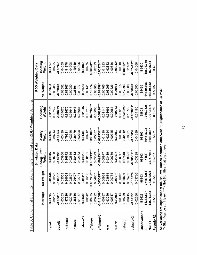
Tabl

e 3:

Con

ditio

nal L

ogit

Estim

atio

n fo

r the

Sim

ulat

ed a

nd R

DD

Wei

ghte

d Sa

mpl

es

Si

mul

ated

Dat

a R

DD

Wei

ghte

d D

ata

In

terc

ept

No

Wei

ght

Endo

g. S

trat

W

eigh

t A

vidi

ty

Wei

ght

Boo

stin

g W

eigh

t N

o W

eigh

t B

oost

ing

Wei

ght

trav

elc

-0.0

1702

-0

.014

35

-0.0

1607

-0

.012

80

-0.0

1521

-0

.016

93

-0.0

1738

0.00

197

0.00

223

0.00

250

0.00

214

0.00

247

0.00

203

0.00

225

trav

elt

-0.8

3616

-0

.886

11

-0.8

9990

-0

.871

42

-0.8

6233

-0

.838

78

-0.6

6940

0.03

003

0.03

553

0.03

900

0.03

439

0.04

075

0.03

092

0.04

655

ln(S

ites)

0.

8732

0 0.

8005

8 0.

8667

2 0.

7982

1 0.

8967

5 0.

8736

7 0.

8197

8

0.02

070

0.02

827

0.02

886

0.02

946

0.03

647

0.02

080

0.04

908

insh

ore

0.28

686

0.26

497

0.28

452

0.26

479

0.25

941

0.26

601

0.19

119

0.

0195

7 0.

0273

1 0.

0266

3 0.

0279

8 0.

0308

1 0.

0197

7 0.

0409

5 in

shor

e^2

-0.0

1583

-0

.014

11

-0.0

1519

-0

.014

00

-0.0

1346

-0

.014

55

-0.0

1065

0.00

142

0.00

206

0.00

191

0.00

212

0.00

215

0.00

141

0.00

275

offs

hore

0.

0993

5 0.

0573

30**

* 0.

0512

19**

* 0.

0901

86**

0.

0452

87**

* 0.

1037

4 0.

0682

0***

0.03

722

0.04

857

0.05

073

0.05

087

0.06

003

0.03

763

0.07

023

offs

hore

^2

-0.0

1858

9*

-.003

545*

**

-0.0

0943

4***

-0

.007

931*

**

-0.0

0629

0***

-0

.018

59*

-0.0

0976

***

0.

0076

7 0.

0095

4 0.

0097

7 0.

0101

0 0.

0114

4 0.

0076

5 0.

0128

3 re

ef

0.03

040

0.03

679

0.03

439

0.02

994

0.03

005

0.03

095

0.02

812

0.

0061

7 0.

0073

5 0.

0078

6 0.

0074

5 0.

0098

1 0.

0062

6 0.

0084

6 re

ef^2

-0

.000

68

-0.0

0071

-0

.000

74

-0.0

0060

-0

.000

63

-0.0

0064

-0

.000

42*

0.

0001

4 0.

0001

6 0.

0001

7 0.

0001

6 0.

0001

8 0.

0001

5 0.

0001

9 pe

lagi

c 0.

1920

9 0.

3060

9 0.

2751

0 0.

4201

2 0.

2452

25*

0.17

293

0.18

066*

**

0.

0641

5 0.

0945

2 0.

0892

1 0.

1038

1 0.

1077

9 0.

0650

0 0.

1118

2 pe

lagi

c^2

-0.0

7135

-0

.107

79

-0.0

8385

1*

-0.1

5059

-0

.089

861*

-0

.069

98

-0.0

7419

**

0.

0256

0 0.

0372

6 0.

0339

8 0.

0428

9 0.

0418

0 0.

0259

0 0.

0406

8

Obs

erva

tions

18

6626

98

803

9880

3 98

803

9880

3 18

5430

18

5430

LL

-1

4332

.527

-7

715.

4251

-7

451

-804

6.83

92

-776

6.95

25

-141

39.7

08

-158

01.7

39

Nul

l LL

-145

91.3

53

-784

6.92

21

-757

4.79

82

-819

3.88

37

-790

7.68

75

-143

49.1

32

-159

96.5

4 Ps

eudo

R2

0.55

6 0.

5556

0.

5757

0.

5352

0.

5575

0.

5565

0.

49

All

Varia

bles

are

sig

nific

ant a

t the

.01

leve

l unl

ess

iden

tifie

d ot

herw

ise;

* - S

igni

fican

ce a

t .05

leve

l;

**

- Sig

nific

ance

at .

1 le

vel;

*** -

Not

Sig

nific

ant a

t the

.1 le

vel

37

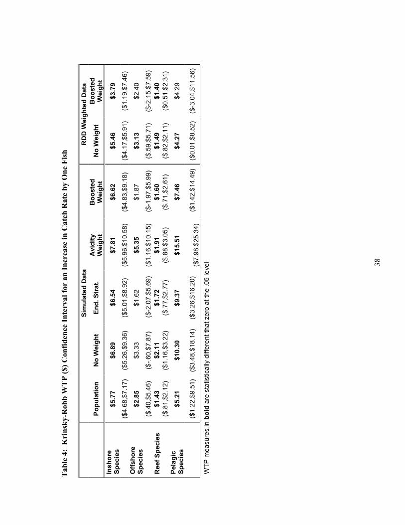
38

Tab

le 4

: K

rins

ky-R

obb

WT

P ($

) Con

fiden

ce In

terv

al fo

r an

Incr

ease

in C

atch

Rat

e by

One

Fis

h

Si

mul

ated

Dat

a

RD

D W

eigh

ted

Dat

a

Po

pula

tion

No

Wei

ght

End.

Str

at.

Avi

dity

W

eigh

t B

oost

ed

Wei

ght

No

Wei

ght

Boo

sted

W

eigh

t In

shor

e Sp

ecie

s $5

.77

$6

.54

$7.8

1

$6.8

9$6

.62

$5.4

6$3

.79

($

4.68

,$7.

17)

($5.

26,$

9.36

) ($

5.01

,$8.

92)

($5.

96,$

10.5

8)($

4.83

,$9.

18)

($4.

17,$

5.91

)($

1.19

,$7.

46)

Offs

hore

Sp

ecie

s $2

.85

$3.3

3 $1

.62

$5.3

5 $1

.87

$3.1

3 $2

.40

($

.40,

$5.4

6)

($-.6

0,$7

.87)

)

($-2

.07,

$5.6

9($

1.16

,$10

.15)

($-1

.97,

$5.9

9)

($.5

9,$5

.71)

($

-2.1

5,$7

.59)

R

eef S

peci

es

$1.4

3

$2

.11

$1.7

2 $1

.91

$1.6

0$1

.49

$1.4

0

($.8

1,$2

.12)

($

1.16

,$3.

22)

) ($

.77,

$2.7

7($

.88,

$3.0

5)

($.7

1,$2

.61)

($

.82,

$2.1

1)

($0.

51,$

2.31

) Pe

lagi

c Sp

ecie

s $5

.21

$7

.46

$4.2

7 $1

0.30

$9.3

7$1

5.51

$4.2

9

($

1.22

,$9.

51)

($3.

48,$

18.1

4)($

3.26

,$16

.20)

($7.

98,$

25.3

4) (

$1.4

2,$1

4.49

) ($

0.01

,$8.

52)

($-3

.04,

$11.

56)

WTP

mea

sure

s in

bol

d ar

e st

atis

tical

ly d

iffer

ent t

hat z

ero

at th

e .0

5 le

vel

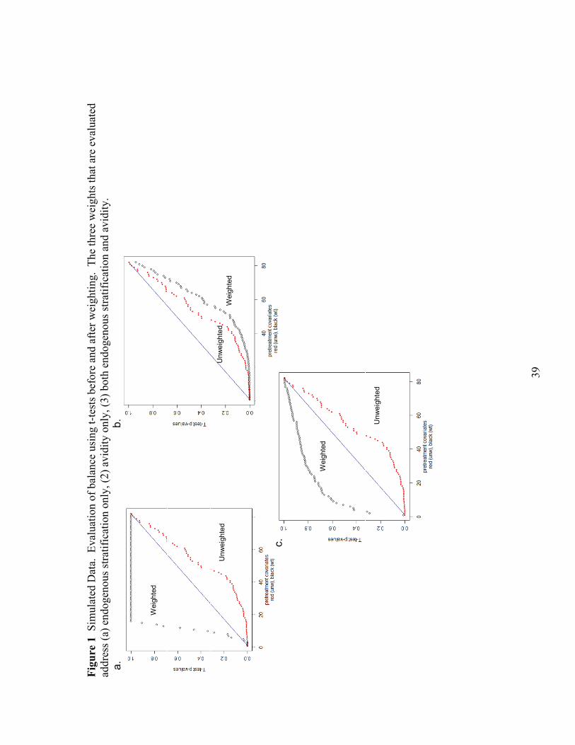
Figu

re 1

Sim

ulat

ed D

ata.

Eva

luat

ion

of b

alan

ce u

sing

t-te

sts b

efor

e an

d af

ter w

eigh

ting.

The

thre

e w

eigh

ts th

at a

re e

valu

ated

ad

dres

s (a)

end

ogen

ous s

tratif

icat

ion

only

, (2)

avi

dity

onl

y, (3

) bot

h en

doge

nous

stra

tific

atio

n an

d av

idity

. a.

b.

c.

Unw

eigh

ted

Wei

ghte

d

Unw

eigh

ted

Wei

ghte

d

Unw

eigh

ted

Wei

ghte

d

39

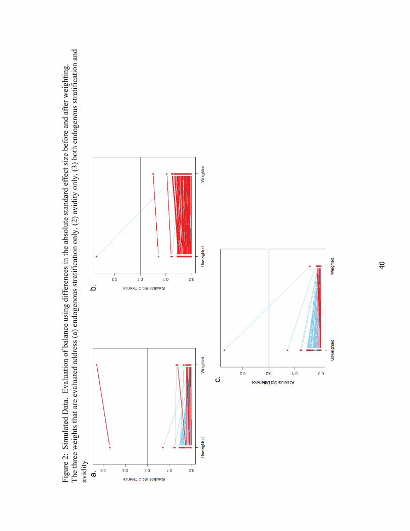
Figu

re 2

: Si

mul

ated

Dat

a. E

valu

atio

n of

bal

ance

usi

ng d

iffer

ence

s in

the

abso

lute

stan

dard

eff

ect s

ize

befo

re a

nd a

fter w

eigh

ting.

Th

e th

ree

wei

ghts

that

are

eva

luat

ed a

ddre

ss (a

) end

ogen

ous s

tratif

icat

ion

only

, (2)

avi

dity

onl

y, (3

) bot

h en

doge

nous

stra

tific

atio

n an

d av

idity

. a.

b.

c.

40

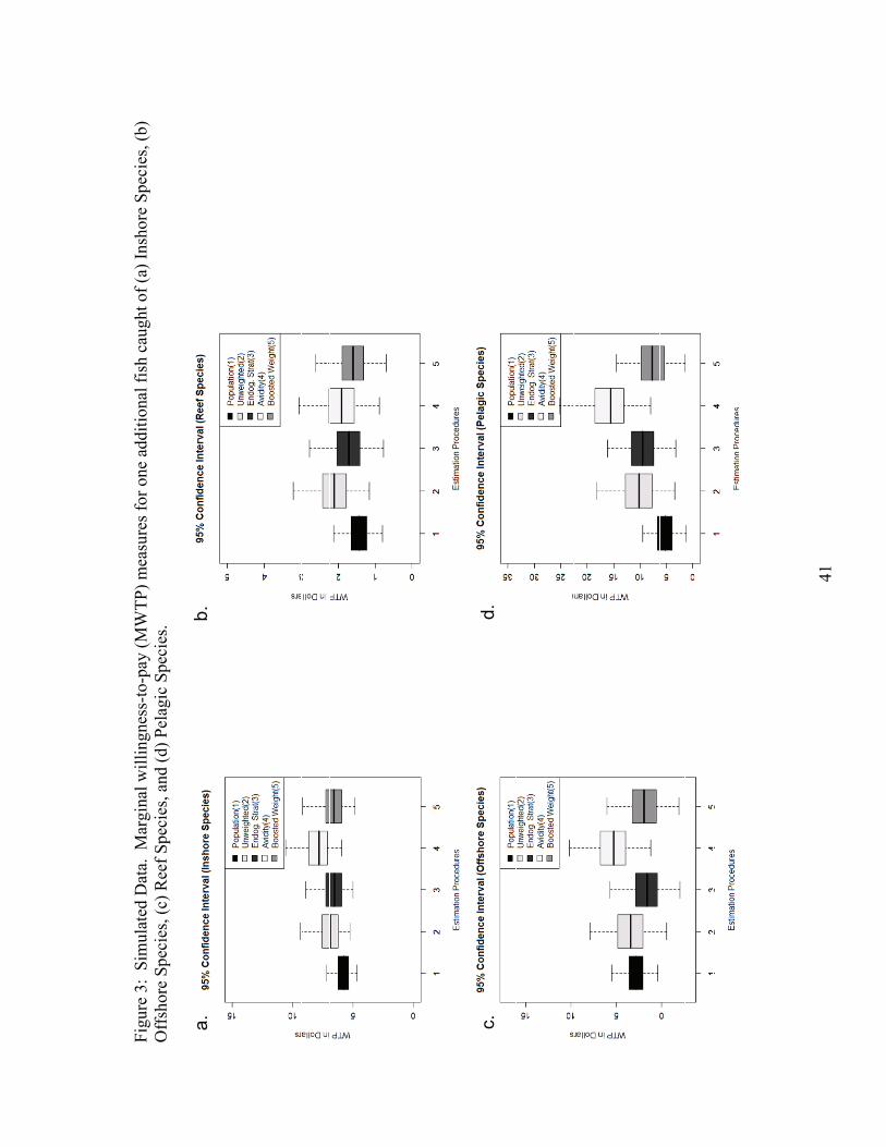
Figu

re 3

: Si

mul

ated

Dat

a. M

argi

nal w

illin

gnes

s-to

-pay

(MW

TP) m

easu

res f

or o

ne a

dditi

onal

fish

cau

ght o

f (a)

Insh

ore

Spec

ies,

(b)

Off

shor

e Sp

ecie

s, (c

) Ree

f Spe

cies

, and

(d) P

elag

ic S

peci

es.

a.b.

c.d.

41

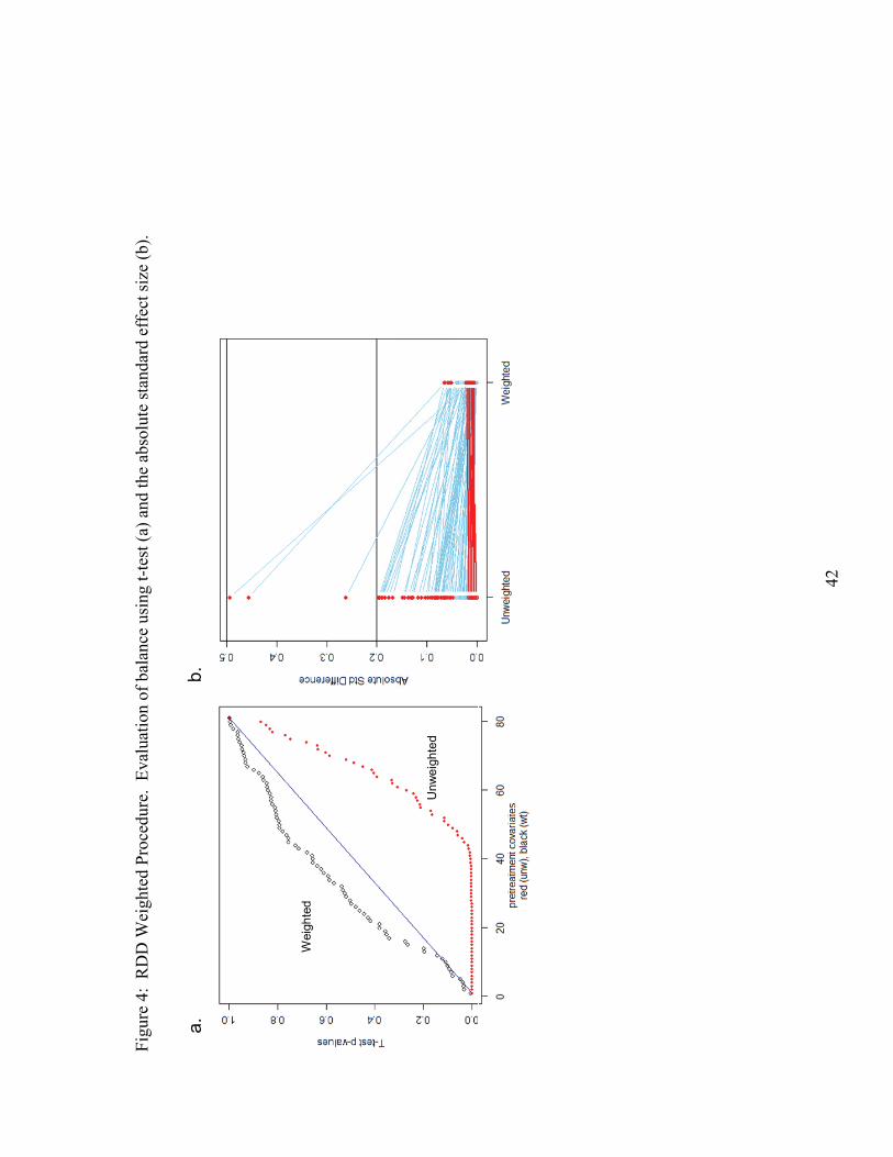
Figu

re 4

: R

DD

Wei

ghte

d Pr

oced

ure.

Eva

luat

ion

of b

alan

ce u

sing

t-te

st (a

) and

the

abso

lute

stan

dard

eff

ect s

ize

(b).

a.b.

Unw

eigh

ted

Wei

ghte

d

42

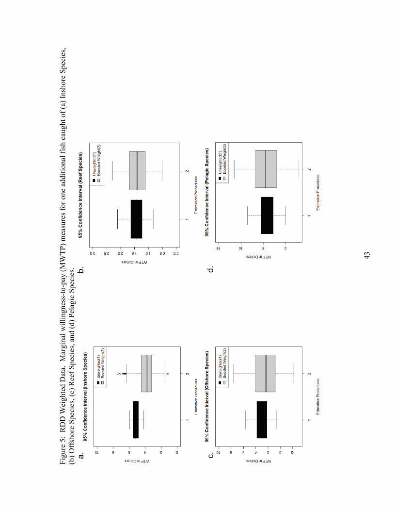
Figu

re 5

: R

DD

Wei

ghte

d D

ata.

Mar

gina

l will

ingn

ess-

to-p

ay (M

WTP

) mea

sure

s for

one

add

ition

al fi

sh c

augh

t of (

a) In

shor

e Sp

ecie

s, (b

) Off

shor

e Sp

ecie

s, (c

) Ree

f Spe

cies

, and

(d) P

elag

ic S

peci

es.

43

c.d.

a.b.