Adaptive dynamics of speciation: ecological underpinnings

Geritz SAH, Kisdi É, Meszéna G & Metz JAJ (2004). Adaptive Dynamics of Speciation: EcologicalUnderpinnings. In: Adaptive Speciation, eds. Dieckmann U, Doebeli M, Metz JAJ & Tautz D, pp. 54–75.

Cambridge University Press. c© International Institute for Applied Systems Analysis

4Adaptive Dynamics of Speciation: Ecological

UnderpinningsStefan A.H. Geritz, Éva Kisdi, Géza Meszéna, and Johan A.J. Metz

4.1 IntroductionSpeciation occurs when a population splits into ecologically differentiated and re-productively isolated lineages. In this chapter, we focus on the ecological side ofnonallopatric speciation: Under what ecological conditions is speciation promotedby natural selection? What are the appropriate tools to identify speciation-proneecological systems?

For speciation to occur, a population must have the potential to become poly-morphic (i.e., it must harbor heritable variation). Moreover, this variation must beunder disruptive selection that favors extreme phenotypes at the cost of intermedi-ate ones. With disruptive selection, a genetic polymorphism can be stable only ifselection is frequency dependent (Pimm 1979; see Chapter 3). Some appropriateform of frequency dependence is thus an ecological prerequisite for nonallopatricspeciation.

Frequency-dependent selection is ubiquitous in nature. It occurs, amongmany other examples, in the context of resource competition (Christiansen andLoeschcke 1980; see Box 4.1), predator–prey systems (Marrow et al. 1992), mul-tiple habitats (Levene 1953), stochastic environments (Kisdi and Meszéna 1993;Chesson 1994), asymmetric competition (Maynard Smith and Brown 1986), mutu-alistic interactions (Law and Dieckmann 1998), and behavioral conflicts (MaynardSmith and Price 1973; Hofbauer and Sigmund 1990).

The theory of adaptive dynamics is a framework devised to model the evolutionof continuous traits driven by frequency-dependent selection. It can be applied tovarious ecological settings and is particularly suitable for incorporating ecologicalcomplexity. The adaptive dynamic analysis reveals the course of long-term evo-lution expected in a given ecological scenario and, in particular, shows whether,and under which conditions, a population is expected to evolve toward a state inwhich disruptive selection arises and promotes speciation. To achieve analyticaltractability in ecologically complex models, many adaptive dynamic models (andmuch of this chapter) suppress genetic complexity with the assumption of clonallyreproducing phenotypes (also referred to as strategies or traits). This enables theefficient identification of interesting features of the engendered selective pressuresthat deserve further analysis from a genetic perspective.

54

4 · Adaptive Dynamics of Speciation: Ecological Underpinnings 55

0

106

–1 +1Strategy, x

Evol

utio

nary

tim

e, t

Figure 4.1 Simulated evolutionary tree for the model described in Box 4.1 with r = 1,K (x) = (1 − x2)+, a(x, x ′) = exp(− 1

2 (x − x ′)2/σ 2a ) with σa = 0.35. The strategy axis

(horizontal) is in arbitrary units; the evolutionary time axis is in units of r−1. For details ofthe simulation, see Geritz et al. (1999) or Kisdi and Geritz (1999).

The analysis begins with the definition of admissible values of the evolvingtraits (including all trade-offs between traits and other constraints upon them), andthe construction of a population dynamic model that incorporates the specific eco-logical conditions to be investigated, along with a specification of how the modelparameters depend on the trait values. From the population dynamic model, onecan derive the fitness of any possible rare mutant in a given resident population. Itis thus possible to deduce which mutants can invade the population, and in whichdirection evolution will proceed via a sequence of successive invasion and fixationevents.

Eventually, directional evolution may arrive at a particular trait value for whicha successful invading mutant does not oust and replace the former resident; instead,the mutant and the resident coexist. If the two strategies coexist, and if selection inthe newly formed dimorphic population is disruptive (i.e., if it favors new mutantsthat are more extreme and suppresses strategies between those of the two resi-dents), then the clonal population undergoes evolutionary branching, whereby thesingle initial strategy is replaced by two strategies separated by a gradually widen-ing gap. Figure 4.1 shows a simulated evolutionary tree with two such branchingevents. With small mutations, such a split can occur when directional evolutionapproaches a particular trait value called a branching point.

Evolutionary branching of clonal strategies cannot be equated with speciation,since clonal models of adaptive dynamics are unable to address the question ofreproductive isolation. Chapter 5 discusses adaptive dynamics with multilocus ge-netics and the emergence of reproductive isolation during evolutionary branching.Yet, evolutionary branching itself signals that adaptive speciation is promoted byselection in the ecological system considered.

In this chapter we outline one particular framework of adaptive dynamics thathas been developed by Metz et al. (1996), Geritz et al. (1997, 1998), and, for direc-tional evolution, Dieckmann and Law (1996). This framework integrates conceptsfrom the modern theory of evolutionarily stable strategies (Maynard Smith 1982;Eshel 1983; Taylor 1989; Nowak 1990; Christiansen 1991) and accommodates

56 A · Theories of Speciation

evolutionary branching. We constrain this summary mainly to a simple graphicapproach; the corresponding analytical treatment (which is indispensable if thetheory is to be applied to multidimensional traits or to polymorphic populationsthat cannot be depicted in simple one- or two-dimensional plots; see Box 4.5) canbe found in Metz et al. (1996) and Geritz et al. (1998).

4.2 Invasion FitnessInvasion fitness is the exponential growth rate of a rare mutant strategy in the en-vironment set by a given resident population (Metz et al. 1992). The calculationof invasion fitness depends on the particular ecological setting to be investigated.Here we sketch the basics of fitness calculations common to all models.

Consider a large and well-mixed population in which a rare mutant strategyappears. The change in the density of mutants can be described by

n(t + 1) = A(E(t))n(t) . (4.1a)

Here n is the density of mutants or, in structured populations, the vector that con-tains the density of mutants in various age or stage classes. The matrix A describespopulation growth as well as transitions between different age or stage classes(Caswell 1989); in an unstructured population, A is simply the annual growth rate.In continuous time, the population growth of the mutant can be described by

dn(t)

dt= B(E(t))n(t) . (4.1b)

The dynamics of the mutant population as specified by A(E) (in discrete time)or B(E) (in continuous time) depends on the properties of the mutant and on theenvironment E . The environment contains all factors that influence populationgrowth, including the abundance of limiting resources, the density of predatorsor parasites, and abiotic factors. Most importantly, E contains all the effects theresident population has directly or indirectly on the mutant; generally, E dependson the population density of the residents. As long as the mutant is rare, its effecton the environment is negligible.

The exponential growth rate, or invasion fitness, of the mutant strategy is de-fined by comparing the total density N (t) of mutants, after a sufficiently longtime, with the initial density N (0), while keeping the mutant’s environment fixed.In structured populations N is the sum of the vector components of n, whereasin unstructured populations there is no difference between the two. Formally, theinvasion fitness is given by (Metz et al. 1992)

f = limt→∞

1

tln

N (t)

N (0). (4.2)

The long time interval is taken to ensure that the population experiences a rep-resentative time series of the possibly fluctuating environment E(t), and that astructured mutant population attains its stationary distribution. For a nonstructuredpopulation in a stable environment (which requires a stable resident population),there is no need to consider a long time interval: the invasion fitness of the mutant


Box 4.1 Invasion fitness in a model of competition for a continuous resource

Consider the Lotka–Volterra competition model

1

ni

dni

dt= r

[1 −

∑j a(xi , xj )nj

K (xi )

], (a)

where the trait value xi determines which part of a resource continuum the i thstrategy can utilize efficiently (e.g., beak size determines which seeds of a con-tinuous distribution of seed sizes are consumed). The more similar two strate-gies are, the more their resources overlap, and the more intense the competi-tion. This can be expressed by the commonly used Gaussian competition functiona(xi , xj ) = exp(− 1

2 (xi − xj )2/σ 2

a ) (see Christiansen and Fenchel 1977). We as-sume that the intrinsic growth rate r is constant and that the carrying capacity Kis unimodal with a maximum at x0; K is given by K (x) = (K0 − λ(x − x0)

2)+,where (...)+ indicates that negative values are set to zero. This model (or a verysimilar model) has been investigated, for example, by Christiansen and Loeschcke(1980), Slatkin (1980), Taper and Case (1985), Vincent et al. (1993), Metz et al.(1996), Doebeli (1996b), Dieckmann and Doebeli (1999), Drossel and McKane(1999), Day (2000), and Doebeli and Dieckmann (2000).

As long as a mutant strategy is rare, its self-competition and impact on the resi-dent strategies are negligible. The density of a rare mutant strategy x ′ thus increasesexponentially according to

1

n′dn′

dt= r

[1 −

∑j a(x ′, xj )n j

K (x ′)

], (b)

where n j is the equilibrium density of the j th resident. These equilibrium densitiescan be obtained by setting Equation (a) equal to zero and solving for ni . The right-hand side of Equation (b) is the exponential growth rate, or invasion fitness, ofthe mutant x ′ in a resident population with strategies x1, ..., xn . Specifically, in amonomorphic resident population with strategy x , the equilibrium density is K (x)

and the mutant’s fitness simplifies to

f (x ′, x) = r

[1 − a(x ′, x)

K (x)

K (x ′)

]. (c)

Figures 4.1 and 4.2, and the figure in Box 4.5, are based on this model.

is then simply f = ln A(E) in discrete time and f = B(E) in continuous time,with E being the environment as set by the equilibrium resident population. Apositive value of f indicates that the mutant strategy can spread in the population,whereas a mutant with negative f will die out. Box 4.1 contains an example ofhow to calculate f for a concrete model.

At the very beginning of the invasion process, typically only a few mutant indi-viduals are present. As a consequence, demographic stochasticity plays an impor-tant role so that the mutant may die out despite having a positive invasion fitnessf . However, the mutant has a positive probability of escaping random extinction


whenever its growth rate f is positive (Crow and Kimura 1970; Goel and Richter-Dyn 1974; Dieckmann and Law 1996). Once the mutant has grown sufficientlyin number so that demographic stochasticity can be neglected, its further inva-sion dynamics is given by Equation (4.1) as long as it is still rare in frequency.Equation (4.1) ceases to hold once the mutant becomes sufficiently common thatit appreciably influences the environment E .

Henceforth the fitness of a rare mutant strategy with trait value x ′ in a residentpopulation of strategy x is denoted by f (x ′, x) to emphasize that the fitness of arare mutant depends on its own strategy as well as on the resident strategy, sincethe latter influences the environment E . This notation suppresses the associatedecological variables, such as the equilibrium density of the residents. It is essentialto realize, however, that the fitness function f (x ′, x) is derived from a popula-tion dynamic model that appropriately incorporates the ecological features of thesystem under study.

4.3 Phenotypic Evolution by Trait SubstitutionA single evolutionary step is made when a new strategy invades the population andousts the former resident. The phenotypes that prevail in the population evolve bya sequence of invasions and substitutions. We assume that mutations occur in-frequently, so that the previously invading mutant becomes established and thepopulation reaches its population dynamic equilibrium (in a deterministic or sta-tistical sense) by the time the next mutant arrives, and also that mutations are ofsmall phenotypic effect (i.e., that a mutant strategy is near the resident strategyfrom which it originated).

Consider a monomorphic resident population with a single strategy x . A mutantstrategy x ′ can invade this population if its fitness f (x ′, x) is positive. If strategy xhas a negative fitness when strategy x ′ is already widespread, then the mutant strat-egy x ′ can eliminate the original resident. We assume that there is no unprotectedpolymorphism and thus infer that strategy x ′ can replace strategy x if and only iff (x ′, x) is positive and f (x, x ′) is negative. On the other hand, if both strategiesspread when rare, that is, if both f (x ′, x) and f (x, x ′) are positive, then the twostrategies form a protected dimorphism.

In the remainder of this section, as well as in Section 4.4, we focus on the evo-lution of strategies specified by a single quantitative trait in monomorphic residentpopulations. To visualize the course of phenotypic evolution it is useful to depictgraphically those mutant strategies that can invade in various resident populationsand those strategy pairs that can form protected dimorphisms. Figure 4.2a showsa so-called pairwise invasibility plot (Matsuda 1985; Van Tienderen and de Jong1986): each point inside the gray area represents a resident–mutant strategy com-bination such that the mutant can invade the population of the resident. Pointsinside the white area correspond to mutant–resident strategy pairs such that themutant cannot invade. A pairwise invasibility plot is constructed by evaluatingthe mutant’s fitness f (x ′, x) for all values of x and x ′ and “coloring” the corre-sponding point of the plot according to whether f (x ′, x) is positive or negative. In


+1–1

+1

–1

+1

+1x*x*

(a) (b)

Mut

ant

stra

tegy

, x′

Stra

tegy

, x′

–1–1Resident strategy, x Strategy, x

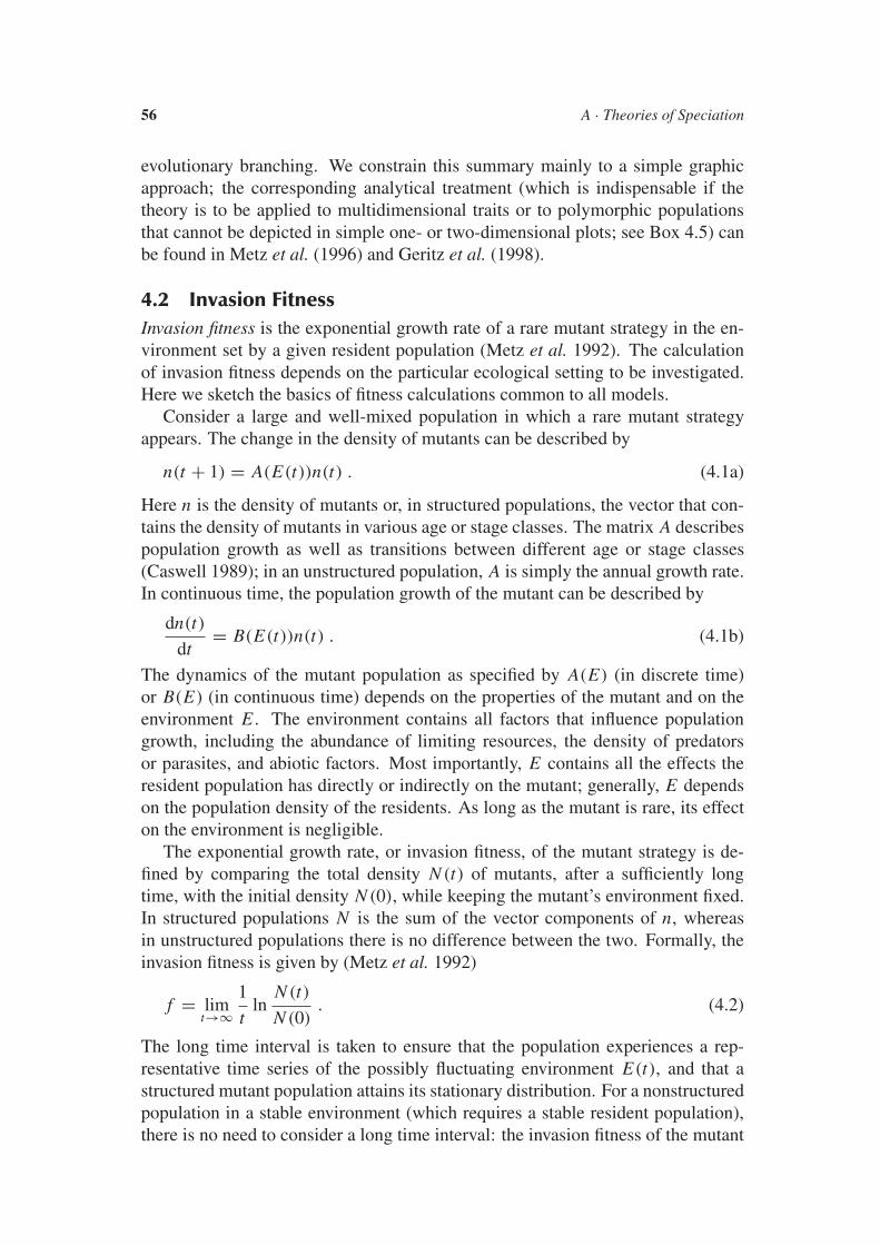
Figure 4.2 Course of phenotypic evolution for the model described in Box 4.1 with r =1, K (x) = (1 − x2)+, a(x, x ′) = exp(− 1

2 (x − x ′)2/σ 2a ) with σa = 0.5. (a) Pairwise

invasibility plot. Gray areas indicate combinations of mutant strategies x ′ and residentstrategies x for which the mutant’s fitness f (x ′, x) is positive; white areas correspond tostrategy combinations such that f (x ′, x) is negative. (b) The set of potentially coexistingstrategies. Gray areas indicate strategy combinations for which both f (x ′, x) and f (x, x ′)are positive; protected coexistence outside the gray areas is not possible. In both (a) and (b),the dotted lines schematically illustrate the narrow band of mutants near the resident thatcan arise by mutations of small phenotypic effect. The singular strategy is denoted by x∗.

Figure 4.2b the gray area indicates that both f (x ′, x) and f (x, x ′) are positive, andhence the two strategies are able to coexist. This plot is obtained by first mirroringthe pairwise invasibility plot along its main diagonal x ′ = x [which amounts to re-versing the roles of the mutant and the resident and gives the sign plot of f (x, x ′)]and then superimposing the mirror image on the original. The overlapping grayareas correspond to strategy pairs that form protected dimorphisms.

With small mutations, x and x ′ are never far apart, so that only a narrow bandalong the main diagonal x ′ = x is of immediate interest. The main diagonal it-self is always a borderline between “invasion” (gray) and “noninvasion” (white)areas, because residents are selectively neutral among themselves, and thereforef (x) = 0 for all x . In Figure 4.2a, resident populations with a trait value less thanx∗ can always be invaded by mutants with slightly larger trait values. Coexistenceis not possible, because away from x∗ any combination of mutant and residentstrategies near the main diagonal lies within the white area of Figure 4.2b. Thus,starting with a trait value left of x∗, the population evolves to the right through aseries of successive substitutions. By the same argument, it follows that a pop-ulation starting on the right of x∗ evolves to the left. Eventually, the populationapproaches x∗, where directional selection ceases. Trait values for which there isno directional selection are called evolutionarily singular strategies (Metz et al.1996; Geritz et al. 1998).

The graphic analysis of Figure 4.2 is sufficient to establish the direction of evo-lution in the case of monomorphic populations in which a single trait is evolving,but gives no explicit information on the speed of evolution. In Box 4.2, we outlinea quantitative approach that assesses the speed of mutation-limited evolution.


Box 4.2 The speed of directional evolution

The speed of mutation-limited evolution is influenced by three factors: how oftena new mutation occurs; how large a phenotypic change this causes; and how likelyit is that an initially rare mutant invades. If the individual mutational steps aresufficiently small, and thus long-term evolution proceeds by a large number of sub-sequent invasions and substitutions, the evolutionary process can be approximatedby the canonical equation of adaptive dynamics (Dieckmann and Law 1996),

dx

dt= 1

2α(x)µ(x)N(x)σ 2

M(x)∂ f (x ′, x)

∂x ′

∣∣∣∣x ′=x

. (a)

Here µ is the probability of a mutation per birth event, and N is the equilibriumpopulation size: the product µN is thus proportional to the number of mutationsthat occur per unit of time. The variance of the phenotypic effect of a mutation isσ 2

M (with symmetric unbiased mutations, the expected phenotypic effect is zero andthe variance measures the size of “typical” mutations). The probability of invasionconsists of three factors. First, during directional evolution, either only mutantswith a trait value larger than the resident, or only mutants with a trait value smallerthan the resident, can invade (see Figure 4.2a); in other words, half of the mutantsare at a selective disadvantage and doomed to extinction. This leads to the factor12 . Second, even mutants at selective advantage may be lost through demographicstochasticity (genetic drift) in the initial phase of invasion, when they are present inonly small numbers. For mutants of small effect, the probability of not being lost isproportional to the selective advantage of the mutant as measured by the fitness gra-dient ∂ f (x ′, x)/∂x ′|x ′=x . Finally, the constant of proportionality α is proportionalto the inverse of the variance in offspring number: with the same expected num-ber of offspring, an advantageous mutant is more easily lost through demographicstochasticity if its offspring number is highly variable. The constant α equals 1for a constant birth–death process in an unstructured population, as considered byDieckmann and Law (1996).

Other models of adaptive dynamics agree that the change in phenotype is pro-portional to the fitness gradient, that is

dx

dt= β

∂ f (x ′, x)

∂x ′

∣∣∣∣x ′=x

(b)

(e.g., Abrams et al. 1993a; Vincent et al. 1993; Marrow et al. 1996). This equa-tion leads to results similar to those from quantitative genetic models (Taper andCase 1992) and, indeed, can be derived as an approximation to the quantitative ge-netic iteration (Abrams et al. 1993b). Equations (a) and (b) have a similar form,though the interpretation of their terms is different: in quantitative genetics, β isthe additive genetic variance and thus measures the standing variation upon whichselection operates; it is often assumed to be constant. In the canonical equation,β depends on the probability and distribution of new mutations; also, β generallydepends on the prevalent phenotype x , if only through the population size N (x).In quantitative genetics, evolutionary change is proportional to the fitness gradient,because stronger selection means faster change in the frequencies of alleles that arepresent from the onset. In mutation-limited evolution, a higher fitness gradient in-creases the probability that a favorable mutant escapes extinction by demographicstochasticity.


x*

(a)

x1 x2

(b) (c)

Mutant strategy, x′

Mut

ant

fitne

ss, f

x1

x2

x3

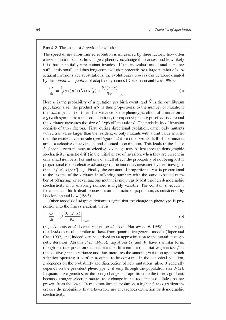
Figure 4.3 Evolutionary branching and a mutant’s fitness as a function of its strategy.(a) Mutant fitness in a monomorphic resident population at a branching point x∗. (b) Mutantfitness in a dimorphic resident population with strategies x1 and x2, both similar to thebranching point x∗. Notice that only those mutants outside the interval spanned by x1 andx2 have a positive fitness and hence can invade. (c) Mutant fitness in a dimorphic residentpopulation with strategies x1 and x3. The former resident x2 now has a negative fitness, andhence is expelled from the population.

4.4 The Emergence of Diversity: Evolutionary BranchingAlthough the evolutionarily singular strategy x∗ in Figure 4.2a is an attractor ofmonomorphic directional evolution, it is not evolutionarily stable in the classicsense (Maynard Smith 1982), that is, it is not stable against invading mutants. Infact, mutants both smaller and larger than x∗ can invade the resident population ofx∗. Unlike in directional evolution, in the neighborhood of x∗ the invasion of a mu-tant results in coexistence of the resident and mutant strategies (Figure 4.2b). Asthe singularity is approached by small but finite mutational steps, the populationactually becomes dimorphic as soon as the next mutant enters the area of coexis-tence (i.e., a little before exactly reaching the singular strategy, Figure 4.2b).

To see how evolution proceeds in the now dimorphic population, it is useful toplot the mutant’s fitness as a function of the mutant trait value (Figure 4.3). Inthe resident population of the singular strategy x∗, all nearby mutants are able toinvade (i.e., they have positive fitness), except for the singular strategy itself, whichhas zero fitness. The fitness function thus attains a minimum at x∗ (Figure 4.3a). Ina dimorphic population with two strategies x1 and x2, both similar to x∗, the fitnessfunction is also similar, but with zeros at x1 and x2, because residents themselvesare selectively neutral (Figure 4.3b).

According to Figure 4.3b, a new mutant that arises in the dimorphic popula-tion with strategies x1 and x2 similar to x∗ has a positive fitness, and thereforecan invade, if and only if it is outside the interval spanned by the two residenttrait values. By contrast, mutants between these values have a negative fitnessand therefore must die out. A mutant cannot coexist with both former resi-dents, because the parabolically shaped fitness function cannot have three zerosto accommodate three established resident strategies. It follows that the success-fully invading mutant will oust the resident that has become the middle strategy(Figure 4.3c).

Since the initial dimorphic population is formed of the most recent monomor-phic resident and its mutant, with small mutations these two strategies are very


Box 4.3 How to recognize evolutionary branching points

One can easily search for evolutionary branching points in a model once the mutantfitness function f (x ′, x) has been determined. If f (x ′, x) is known analytically,then the following criteria must be satisfied by an evolutionary branching point x∗

(Geritz et al. 1998):

1. x∗ must be an evolutionary singularity, i.e., the fitness gradient vanishes at x∗,

∂ f (x ′, x)

∂x ′

∣∣∣∣x ′=x=x∗

= 0 . (a)

2. x∗ must be an attractor of directional evolution (Eshel 1983),

∂2 f (x ′, x)

∂x∂x ′ + ∂2 f (x ′, x)

∂x ′2

∣∣∣∣x ′=x=x∗

< 0 . (b)

3. In the neighborhood of x∗, similar strategies must be able to form protecteddimorphisms (Geritz et al. 1998),

∂2 f (x ′, x)

∂x2+ ∂2 f (x ′, x)

∂x ′2

∣∣∣∣x ′=x=x∗

> 0 . (c)

4. x∗ must lack evolutionary stability (Maynard Smith 1982), which ensures dis-ruptive selection at x∗ (Geritz et al. 1998),

∂2 f (x ′, x)

∂x ′2

∣∣∣∣x ′=x=x∗

> 0 . (d)

As can be verified by inspection of all the generic singularities (see Box 4.4), thesecond-order criteria (2)–(4) are not independent for the case of a single trait and aninitially monomorphic resident population; instead, criteria (2) and (4) are sufficientto ensure (3) as well. This is, however, not true for multidimensional strategiesor for coevolving populations (Geritz et al. 1998). These criteria are thus bestremembered separately.

Alternatively, a graphic analysis can be performed using a pairwise invasibilityplot (Figure 4.2a). Although drawing the pairwise invasibility plot is practical onlyfor the case of single traits and monomorphic populations, it is often used when theinvasion fitness cannot be determined analytically. In a pairwise invasibility plot,the evolutionary branching point is recognized by the following pattern:

� The branching point is at a point of intersection between the main diagonal andanother border line between positive and negative mutant fitness.

� The fitness of mutants is positive immediately above the main diagonal to theleft of the branching point and below the main diagonal to its right.

� Potentially coexisting strategies lie in the neighborhood of the branching point(this can be checked on a plot similar to Figure 4.2b, but, as highlighted above,in the simple case for which pairwise invasibility plots are useful, this criteriondoes not have to be checked separately).

� Looking along a vertical line through the branching point, the mutants immedi-ately above and below are able to invade.


Box 4.4 Types of evolutionary singularities

Eight types of evolutionary singularities occur generically in single-trait evolutionof monomorphic populations, as in the figure below (Geritz et al. 1998). As in Fig-ure 4.2a, gray areas indicate combinations of mutant strategies and resident strate-gies for which the mutant’s fitness is positive.

(a)

(b)

(c)

Resident strategy, x

Mut

ant

stra

tegy

, x′

These types can be classified into three major groups:

� Evolutionary repellors, (a) in the figure above. Directional evolution leads awayfrom this type of singularity, and therefore these types do not play a role asevolutionary outcomes. If the population has several singular strategies, then arepellor separates the basins of attraction of adjacent singularities.

� Evolutionary branching points, (b) in the figure above. This type of singular-ity is an attractor of directional evolution, but it lacks evolutionary stability andtherefore evolution cannot stop here. Invading mutants give rise to a protecteddimorphism in which the constituent strategies are under disruptive selectionand diverge away from each other. Evolution can enter a higher level of poly-morphism by small mutational steps only via evolutionary branching.

� Evolutionarily stable attractors, (c) in the figure above. Singularities of this typeare attractors of directional evolution and, moreover, once established the popu-lation cannot be invaded by any nearby strategy. Such strategies are also calledcontinuously stable strategies (Eshel 1983). Coexistence of strategies may bepossible, but coexisting strategies undergo convergent rather than divergent co-evolution such that eventually the dimorphism disappears. Evolutionarily stableattractors act as final stops of evolution.

similar. After the first substitution in the dimorphic population, however, the newresident population consists of two strategies with a wider gap between. Through aseries of such invasions and replacements, the two strategies of the dimorphic pop-ulation undergo divergent coevolution and become phenotypically clearly distinct(see Figure 4.1).

The process of convergence to a particular trait value in the monomorphic pop-ulation followed by gradual divergence once the population has become dimorphic


Box 4.5 Polymorphic and multidimensional evolution

If the theory of adaptive dynamics were only applicable to the caricature of one-dimensional trait spaces or monomorphic populations, it would be of very limitedutility. Below we therefore describe how this framework can be extended.

We start by considering polymorphic populations. By assuming mutation-limited evolution we can ignore the possibility of simultaneous mutations that occurin different resident strategies. Two strategies x1 and x2 can coexist as a protecteddimorphism if both f (x2, x1) and f (x1, x2) are positive (i.e., when both can invadeinto a population of the other). For each pair of resident strategies x1 and x2 we canconstruct a pairwise invasibility plot for x1 while keeping x2 fixed, and a pairwiseinvasibility plot for x2 while keeping x1 fixed. From this we can see which mutantsof x1 or of x2 could invade the present resident population and which could not (i.e.,in what direction x1 and x2 will evolve by small mutational steps).

In the example shown in the figure below, the arrows indicate the directions ofevolutionary change in x1 and in x2. On the lines that separate regions with differentevolutionary directions, selection in one of the two resident strategies is no longerdirectional: each point on such a line is a singular strategy for the correspondingresident, if the other resident is kept fixed. The points of these lines, therefore,can be classified similarly to the monomorphic singularities in Box 4.4. Within theregions of coexistence in the figure below continuous lines indicate evolutionarystability and dashed lines the lack thereof. At the intersection point of two suchlines, directional evolution ceases for both residents. Such a strategy combinationis called an evolutionarily singular dimorphism. This dimorphism is evolutionarilystable if neither mutants of x1 nor mutants of x2 can invade (i.e., if both x1 and x2

are evolutionarily stable); in the figure this is the case.continued

Strategy, x1

Stra

tegy

, x2

+1

+1

x*x*1–1

–1

x2*

x2*

x*1

Adaptive dynamics in a dimorphic population for the model described in Box 4.1 withr = 1, K (x) = (1 − x2)+, and σa = 0.5. Gray areas indicate strategy pairs (x1, x2) thatcan coexist as a protected dimorphism. Lines inside the gray areas separate regions withdifferent evolutionary directions for the two resident strategies, as illustrated by arrows.On the steeper line, which separates strategy pairs evolving either toward the left ortoward the right, directional evolution in x1 ceases. Likewise, on the shallower line,which separates strategy pairs evolving upward from those evolving downward, direc-tional evolution in x2 ceases. Continuous lines indicate that the corresponding strategyis evolutionarily stable if evolution in the other strategy is arrested. After branching atthe branching point x∗ (open circle), the population evolves into the gray area towardthe evolutionarily stable dimorphism (x∗

1 , x∗2 ) (filled circles), where directional evolution

ceases in both strategies and both strategies also possess evolutionary stability.


Box 4.5 continued

For a singular dimorphism to be evolutionarily attracting it is neither necessary norsufficient that both strategies are attracting if the other resident is kept fixed at itspresent value (Matessi and Di Pasquale 1996; Marrow et al. 1996). With smallevolutionary steps, we can approximate the evolutionary trajectories by utilizingthe canonical equation (see Box 4.2) simultaneously for both coevolving strate-gies. Stable equilibria of the canonical equation then correspond to evolutionarilyattracting singular dimorphisms. If such a dimorphism is evolutionarily stable, itrepresents a final stop of dimorphic evolution. However, if one of the residentstrategies at the singularity is not evolutionarily stable and, moreover, if this resi-dent can coexist with nearby mutants of itself, the population undergoes a secondarybranching event, which leads to a trimorphic resident population (Metz et al. 1996;Geritz et al. 1998). An example of such a process is shown in Figure 4.1.

Next we consider the adaptive dynamics framework in the context of multidi-mensional strategies. In natural environments, strategies are typically characterizedby several traits that jointly influence fitness and that may be genetically correlated.

Though much of the basic framework can be generalized to multidimensionalstrategies, these also pose special difficulties. For example, unlike in the case ofscalar strategies, a mutant that invades a monomorphic resident population maycoexist with the former resident also away from any evolutionary singularity. Thiscoexistence, however, is confined to a restricted set of mutants, such that its volumevanishes for small mutational steps proportionally to the square of the average sizeof mutations. With this caveat, directional evolution of two traits in a monomorphicpopulation can be depicted graphically in a similar way to coevolving strategies.There are two important differences, however. First, the axes of the figure on theprevious page no longer represent different residents, but instead describe differentphenotypic components of the same resident phenotype. Second, if the traits aregenetically correlated such that a single mutation can affect both traits at the sametime, then the evolutionary steps are not constrained to being either horizontal orvertical. Instead, evolutionary steps are possible in any direction within an angle ofplus or minus 90 degrees from the selection gradient vector ∂ f (x ′, x)/∂x ′|x ′=x .

For small mutational steps, the evolutionary trajectory can be approximated by amultidimensional equivalent of the canonical equation (Dieckmann and Law 1996;see Box 4.2), where dx/dt and ∂ f (x ′, x)/∂x ′|x ′=x are vectors, and the mutationalvariance is replaced by the mutation variance–covariance matrix C(x) (the diago-nal elements of this matrix contain the trait-wise mutational variances and the off-diagonal elements represent the covariances between mutational changes in twodifferent traits that may result from pleiotropy). With large covariances, it is pos-sible that a trait changes “maladaptively”, that is, the direction of the net change isopposite to the direct selection on the trait given by the corresponding componentof the fitness gradient (see also Lande 1979b).

An evolutionarily singular strategy x∗, in which all components of the fitnessgradient are zero, is evolutionarily stable if it is, as a function of the traits of themutant strategy x ′, a multidimensional maximum of the invasion fitness f (x ′, x∗).If such a singularity lacks evolutionary stability, evolutionary branching may occur.


Box 4.6 The geography of speciation

Evolutionary branching in a spatially subdivided population based on a simplemodel by Meszéna et al. (1997) is illustrated here. Two habitats coupled by mi-gration are considered. Within each habitat, the population follows logistic growth,in which the intrinsic growth rate is a Gaussian function of strategy, with differentoptima in the two habitats. The model is symmetric, so that the “generalist” strat-egy, which is exactly halfway between the two habitat-specific optima, is alwaysan evolutionarily singular strategy. Depending on the magnitude of the difference� between the local optima relative to the width of the Gaussian curve and onthe migration rate m, this central singularity may either be an evolutionarily stablestrategy, a branching point, or a repellor [(a) in the figure below; see also Box 4.4].

Stra

tegy

, x

–1

1

0 15

x*

1/m1 1/m2 1/m3

x2

x1

15

Patc

h di

ffer

ence

, ∆

00

3

Repellor

Branching point

Evolutionarilystable strategy

Inverse migration rate, 1/m

(a) (b)

Evolutionary properties of singularities in a two-patch model with local adaptation andmigration. (a) A generalist strategy that exploits both patches is an evolutionary repellor,a branching point, or an evolutionarily stable attractor, depending on the difference � be-tween the patch-specific optimal strategies and the migration rate m, as indicated by thethree different parameter regions. (b) Evolutionary singularities as a function of inversemigration rate. The difference between the patch-specific optimal strategies was fixedat � = 1.5. For comparison, the two thin dotted horizontal lines at x1 and x2 denotethe local within-patch optimal strategies (x = ±�/2). Monomorphic singular strategiesare drawn with lines of intermediate thickness, of which the continuous lines correspondto evolutionarily stable attractors, the dashed lines to branching points, and the dottedline to an evolutionary repellor. The monomorphic generalist strategy is indicated by x∗.Along a cross-section at � = 1.5 in (a), indicated by an arrow head, the generalist strat-egy changes with increasing 1/m from an evolutionarily stable attractor into a branchingpoint and then into an evolutionary repellor. The two branches of the bold line indicatethe strategies of the evolutionarily stable dimorphism. Source: Meszéna et al. (1997).

There are four possible evolutionary scenarios [(b) in the figure above]: at highlevels of migration (inverse migration rate smaller than 1/m1), the population ef-fectively experiences a homogeneous environment in which the generalist strategyis evolutionarily stable and branching is not possible. With a somewhat lower mi-gration rate (inverse migration rate between 1/m1 and 1/m2), the generalist is atan evolutionary branching point, and the population evolves to a dimorphism thatconsists of two habitat specialists. Decreasing migration further (inverse migrationrate between 1/m2 and 1/m3), the generalist becomes an evolutionary repellor, but

continued


Box 4.6 continued

there are two additional monomorphic singularities, one on each side of the gener-alist, both of which are branching points. Finally, in case of a very low migrationrate (inverse migration rate greater than 1/m3), these two monomorphic attractorsare evolutionarily stable and branching does not occur, even though there also ex-ists an evolutionarily stable dimorphism of habitat specialists. (A similar sequenceof transitions can be observed if, instead of decreasing the migration rate, the dif-ference between the habitats is increased.) Evolutionary branching is also possibleif the environment forms a gradient instead of discrete habitats, provided there aresufficiently different environments along the gradient and mobility is not too high(Mizera and Meszéna 2003; Chapter 7).

is called evolutionary branching. The singularity at which this happens (x∗ in Fig-ure 4.2a) is an evolutionary branching point. In Box 4.3 we summarize how torecognize branching points by investigating the fitness function f (x ′, x).

The evolutionary branching point, though perhaps the most interesting with re-gard to speciation, is not the only type of singular strategy. In Box 4.4 we brieflysummarize the basic properties of all singularities that occur generically. Through-out this section, we constrain our discussion to single-trait evolution in an initiallymonomorphic population. A brief summary on how to extend these results to poly-morphic populations (including further branching events as in Figure 4.1) and tomultiple-trait evolution is given in Box 4.5; more details can be found in Metzet al. (1996) and Geritz et al. (1998, 1999), and, concerning directional evolution,in Dieckmann and Law (1996), Matessi and Di Pasquale (1996), Champagnat et al.(2001), and Leimar (2001 and in press).

For the adaptive dynamics framework to be applicable to spatially subdividedpopulations, sufficient dispersal must occur between subpopulations for the sta-tionary population distribution to be attained on an ecological time scale. Fullsympatry is, however, by no means a necessary condition, and the framework hasbeen used to analyze evolution in spatially structured populations as well (e.g.,Meszéna et al. 1997; Day 2000; see Box 4.6).

So far we have considered clonally inherited phenotypes. The very same modelcan be applied, however, to the evolution of alleles at a single diploid locus in aMendelian population [Box 4.7; Kisdi and Geritz 1999; see also Christiansen andLoeschcke (1980) for a related approach] when assuming that a continuum of alleletypes is possible, and that the mutant allele codes for a phenotype similar to that ofthe parent allele. Evolutionary branching in alleles then occurs similarly to clonalphenotypes and produces two distinct allele types that may continue to segregatewithin the species. Since intermediate heterozygotes are at a disadvantage underdisruptive selection, selection occurs for dominance and for assortative mating(Udovic 1980; Wilson and Turelli 1986; Van Dooren 1999; Geritz and Kisdi 2000).


Box 4.7 Adaptive dynamics of alleles and stable genetic polymorphisms

As an example for the adaptive dynamics of alleles, consider the classic soft-selection model of Levene (1953; see Box 3.1). We assume that not just two al-leles may segregate (A and a, with fixed selection coefficients s1 and s2), as in theclassic models, but instead that many different alleles may arise by mutations andthat they determine a continuous phenotype in an additive way (i.e., if the pheno-types of AA and aa are, respectively, xA and xa, then the heterozygote phenotype is(xA +xa)/2). Within each habitat, local fitness is a function of the phenotype: ϕi (x)

in habitat i . For example, in the first habitat local fitness values are WAA = ϕ1(xA),WAa = ϕ1((xA + xa)/2), and Waa = ϕ1(xa). For any two alleles A and a, drawnfrom the assumed continuum, the dynamics and equilibrium of allele frequenciescan be obtained as described in Box 3.1. In particular, the frequency of a rare mu-tant allele a increases in a population monomorphic for allele A at a per-generationrate of k1ϕ1((xA + xa)/2)/ϕ1(xA) + k2ϕ2((xA + xa)/2)/ϕ2(xA), where ki is the rel-ative size of habitat i , with k1 + k2 = 1. If this expression is greater than 1 [or,equivalently, if its logarithm, f (xa, xA) in the notation of the main text, is positive],then the mutant allele can invade.

Assuming that mutations only result in small phenotypic change (xa is near xA),we can apply the adaptive dynamics framework to the evolution of alleles (Geritzet al. 1998). Invasion by a mutant allele usually leads to substitution (i.e., thenew allele replaces the former allele, just as in clonal adaptive dynamics). The en-suing directional evolution, however, leads to singular alleles in which protectedpolymorphisms become possible. Evolutionary branching of alleles means that thehomozygote phenotypes diverge from each other, and results in a genetic polymor-phism of distinctly different alleles that segregate in a randomly mating population(Kisdi and Geritz 1999).

Assuming a more flexible genetic variation sheds new light on the old questionof whether stable genetic polymorphisms are sufficiently robust to serve as a basisfor sympatric speciation. Recall from Box 3.1 that if selection coefficients si aresmall, then polymorphism is possible only in a very narrow range of parameters (theparameter region that allows for polymorphism actually has a cusp at s1 = s2 = 0).Given two arbitrary alleles A and a, and therefore given selection coefficients s1

and s2, polymorphism results only if the environmental parameters, in this casethe relative habitat sizes k1 and k2 = 1 − k1, are fine-tuned. This means that apolymorphism of two particular alleles is not robust under weak selection (MaynardSmith 1966; Hoekstra et al. 1985), and this property appeared a significant obstacleto sympatric speciation.

By contrast, the assumption of more flexible genetic variation (a potential con-tinuum of alleles rather than only two alleles) considerably facilitates the evolutionof stable genetic polymorphisms. Here we focus on polymorphisms of similar alle-les (which may arise by a single mutation at the onset of evolutionary branching);this immediately implies that the selection coefficients are small and that the twoalleles cannot form a polymorphism without fine-tuning of the environmental pa-rameters. With many potential alleles, however, the requirement of fine-tuning maybe turned around: given a certain environment (k1 and k2), polymorphism will re-sult if the alleles are chosen from a narrow range. This narrow range turns out to

continued


Box 4.7 continued

coincide with the neighborhood of an evolutionarily singular allele. Thus, startingwith an arbitrary allele A, population genetics and adaptive dynamics agree in thatthe invasion of a mutant allele a usually results in substitution rather than poly-morphism. Repeated substitutions, however, lead toward a singular allele, in theneighborhood of which stable polymorphisms are possible. In other words, evo-lution by small mutational steps proceeds exactly toward those exceptional allelesthat can form polymorphisms: long-term evolution itself takes care of the neces-sary fine-tuning (Kisdi and Geritz 1999; see figure below). If the singularity is abranching point, then the population not only becomes genetically polymorphic,but also is subject to disruptive selection, as is necessary for sympatric speciation.Of course, it remains to be seen whether reproductive isolation can evolve [seeChapters 3 and 5 and references therein; see also Geritz and Kisdi (2000) for ananalysis of the evolution of reproductive isolation through the adaptive dynamics ofalleles]. Fine-tuning is necessary not only in multiple-niche polymorphisms [suchas Levene’s (1953) model and its variants, see Hoekstra et al. (1985)], but also inany generic model in which frequency dependence can maintain protected poly-morphisms; long-term evolution then provides the necessary fine-tuning whenevermany small mutations incrementally change an evolving trait.

(a) (b) (c)

k1 k1

xA

xa

xa – xA xa – xA

00 1 0 11

1

–1–1

1

0

1

*

Allele pairs that can form a stable polymorphism in Levene’s soft selection model withstabilizing selection within each habitat (ϕi is Gaussian with unit width and the twopeaks are located at a distance of � = 3). (a) An arbitrary allele xA = 0.3 can forma polymorphism with allele xa within the shaded area. Notice that if xa − xA is small(i.e., if the two alleles produce similar phenotypes and hence selection is weak), thenpolymorphism is possible only in a narrow range of the environmental parameter k1(fine-tuning). In one particular environment k1 = 0.5 (indicated by arrowheads in the leftand right panels), the allele xA = 0.3 cannot form a polymorphism under weak selection.(b) The set of allele pairs that can form polymorphisms in the particular environmentk1 = 0.5. The thick line corresponds to identical alleles xa = xA; similar alleles withsmall difference xa − xA thus lie in the neighborhood of the thick line. Again, the allelexA = 0.3 (denoted by an asterisk) cannot form a polymorphism with alleles similar toitself in this particular environment. Allele substitutions in the monomorphic population,however, lead to the evolutionary singular allele x∗ = 0, where similar alleles are ableto form polymorphisms in this particular environment. (c) With xA = x∗, the narrowrange of k1 that permits polymorphism with small xa − xA shifts to the actual value ofthe environmental parameter, k1 = 0.5. Note that x∗ depends on the actual value ofthe environmental parameter; it happens to be the central strategy only for the particularchoice k1 = 0.5.


4.5 Evolutionary Branching and SpeciationThe phenomenon of evolutionary branching in clonal models may appear verysuggestive of speciation. First, there is directional evolution toward a well-definedtrait value, the evolutionary branching point. As evolution reaches the branchingpoint, selection turns disruptive. The population necessarily becomes dimorphic inthe neighborhood of the branching point, and disruptive selection causes divergentcoevolution in the two coexisting lineages. The resultant evolutionary pattern is ofa branching evolutionary tree, with phenotypically distinct lineages that developgradually by small evolutionary steps (Figure 4.1).

Naturally, clonal models of adaptive dynamics are unable to account for the ge-netic details of speciation, in particular how reproductive isolation might developbetween the emerging branches (see Dieckmann and Doebeli 1999; Drossel andMcKane 2000; Geritz and Kisdi 2000; Matessi et al. 2001; Meszéna and Chris-tiansen, unpublished; see Chapter 5). What evolutionary branching does imply isthat there is evolution toward disruptive selection and, at the same time, towardpolymorphism in the ecological model in which branching is found. These are theecological prerequisites for speciation and set the selective environment for theevolution of reproductive isolation. Evolutionary branching thus indicates that theecological system under study is prone to speciation.

Speciation by disruptive selection has previously been considered problematic,because disruptive selection does not appear to be likely to occur for a long timeand does not appear to be compatible with the coexistence of different types (eitherdifferent alleles or different clonal types or species). For disruptive selection to oc-cur, the population must be at the bottom of a fitness valley (similar to Figure 4.3).In simple, frequency-independent models of selection, the population “climbs” to-ward the nearest peak of the adaptive landscape (Wright 1931; Lande 1976). Thefitness valleys are thus evolutionary repellors: the population is unlikely to expe-rience disruptive selection, except possibly for a brief exposure before it evolvesaway from the bottom of the valley.

As pointed out by Christiansen (1991) and Abrams et al. (1993a), evolution byfrequency-dependent selection often leads to fitness minima. Even though in eachgeneration the population evolves “upward” on the fitness landscape, the land-scape itself changes such that the population eventually reaches the bottom of avalley. This is what happens during directional evolution toward an evolutionarybranching point.

Disruptive selection has also been thought incompatible with the maintenanceof genetic variability (e.g., Ridley 1993). In simple one-locus models disruptiveselection amounts to heterozygote inferiority, which, in the absence of frequencydependence, leads to the loss of one allele. This is not so under frequency depen-dence (Pimm 1979): at the branching point, the heterozygote is inferior only whenboth alleles are sufficiently common. Should one of the alleles become rare, thefrequency-dependent fitness of the heterozygote increases such that it is no longerat a disadvantage, and therefore the frequency of the rare allele increases again.


Except for asexual species, evolutionary branching corresponds to speciationonly if reproductive isolation emerges between the nascent branches. There aremany ways by which reproductive isolation could, in principle, evolve during evo-lutionary branching (see Chapter 3). Assortative mating based on the same eco-logical trait that is under disruptive selection automatically leads to reproductiveisolation as the ecological trait diverges (Drossel and McKane 2000), and this pos-sibility appears to be widespread in nature (e.g., Chown and Smith 1993; Woodand Foote 1996; Macnair and Gardner 1998; Nagel and Schluter 1998; Grant et al.2000). For example, in the apple maggot fly Rhagoletis pomonella, there is disrup-tive selection on eclosion time; different timing of reproduction helps to preventhybridization between the host races (Feder 1998; see Chapter 11). If differencesin the ecological trait are associated with different habitats, as is the case for the ap-ple maggot fly, then reduced migration, habitat fidelity, or habitat choice ensuresassortative mating (Balkau and Feldman 1973; Diehl and Bush 1989; Kawecki1996, 1997). Assortative mating based on a neutral “marker” trait (e.g., differentflower colors that attract different pollinators) can lead to reproductive isolationbetween the emerging branches only if an association (linkage disequilibrium) isestablished between the ecological trait and the marker. This is considered to bedifficult because of recombination (Felsenstein 1981; but see Dieckmann and Doe-beli 1999; Chapter 5), and possible only if there is strong assortativeness, strongselection on the ecological trait, or low recombination (Udovic 1980; Kondrashovand Kondrashov 1999; Geritz and Kisdi 2000).

The degree of assortativeness in any mate choice system may be sufficientlyhigh at the onset, or else it may increase evolutionarily while the population isat a branching point. Since disruptive selection acts against intermediate pheno-types, assortative mating between phenotypically similar individuals is selectivelyfavored at the branching point. Adaptive increase of assortativeness may be sus-pected if mating is more discriminative in sympatry (Coyne and Orr 1989, 1997;Noor 1995; Sætre et al. 1997) or if some unusual preference appears as a de-rived character (Rundle and Schluter 1998). In models, increased assortativenessreadily evolves if it amounts to the substitution of the same allele in the entire pop-ulation [a “one-allele mechanism” in the sense of Felsenstein (1981)], such as anallele for increased “choosiness” when selecting mates based on the ecological trait(Dieckmann and Doebeli 1999; Chapter 5; but see Matessi et al. 2001; Meszénaand Christiansen, unpublished) or on an allele for reduced migration (Balkau andFeldman 1973). By contrast, two-allele mechanisms depend on the replacementof different alleles in the two branches and thus involve the emergence of linkagedisequilibria, a process counteracted by recombination (Felsenstein 1981). Yetsuch mechanisms have been shown to evolve under certain conditions: when dif-ferent alleles in the two branches code for different habitat preferences, the pro-cess is aided by spatial segregation (Diehl and Bush 1989; Kawecki 1996, 1997),and when the different alleles code for ecologically neutral marker traits, linkagedisequilibria can arise from the deterministic amplification of genetic drift in finitepopulations (Dieckmann and Doebeli 1999; see Chapter 5). Partial reproductive


isolation by one mechanism facilitates the evolution of other isolating mechanisms(Johnson et al. 1996b), whereby the remaining gene flow is further reduced andthe divergent subpopulations attain species rank.

Alternatively, reproductive isolation may arise for reasons independent of dis-ruptive natural selection on the ecological trait. Such mechanisms include sex-ual selection (Turner and Burrows 1995; Payne and Krakauer 1997; Seehausenet al. 1997; Higashi et al. 1999) and the evolution of gamete-recognition systems(Palumbi 1992). If the emergent species experience directional or stabilizing natu-ral selection, they remain ecologically undifferentiated and hence they are unlikelyto coexist for a long time. Evolutionary branching, however, can latch on such thatthe two species evolve into two branches, which ensures the ecological differenti-ation necessary for long-term coexistence (Galis and Metz 1998; Van Doorn andWeissing 2001). Once reproductive isolation has been established between thebranches in any way, further coevolution of the species proceeds as in the clonalmodel of adaptive dynamics.

4.6 Adaptive Dynamics: Alternative ApproachesIn this chapter, we concentrate on the adaptive dynamics framework developedby Metz et al. (1996) and Geritz et al. (1997, 1998). This is by no means theonly approach to adaptive dynamics [see Abrams (2001a) for a review]. We focuson this particular approach because the concept of evolutionary branching mayhelp in the study of nonallopatric speciation. Alternative approaches consider thenumber of species fixed [and hence do not consider speciation at all; see Abrams(2001a) for references to many examples], or assume invasions of new speciesfrom outside the system [the invading species in such cases may be considerablydifferent from the members of the present community and its phenotype is moreor less arbitrary; e.g., Taper and Case (1992)], or establish that polymorphism willoccur at fitness minima, but do not investigate the subsequent coevolution of theconstituent strategies (e.g., Brown and Pavlovic 1992). An important exceptionis the work of Eshel et al. (1997), which paralleled some results of Metz et al.(1996) and Geritz et al. (1997, 1998). A recent paper by Cohen et al. (1999) givessimilar results to those presented in this chapter. This approach uses differentialequations to describe the convergence to the branching point in a monomorphicpopulation and divergence in a dimorphic population; to incorporate the transitionfrom monomorphism to dimorphism, the model has to be modified by adding anew equation at the branching point (see, however, Abrams 2001b). Most modelsof adaptive dynamics agree on the basic form of the equation that describes within-species phenotypic change over time [see Box 4.2, Equation (b)].

In the present framework, analytical tractability comes at the cost of assumingmutation-limited evolution, that is, assuming mutations that occur infrequentlyand, if successful, sweep through the population before the next mutant comesalong. Simulations of the evolutionary process (similar to that shown in Figure 4.1,but with variable size and frequency of mutations) demonstrate that the qualitativepatterns of monomorphic evolution and evolutionary branching are robust with


respect to relaxing this assumption. With a higher frequency of mutations, thenext mutant arises before the previous successful mutant has become fixed, andtherefore there is always some variation in the population. The results are robustwith respect to this variation because the environment, E in Equations (4.1a) and(4.1b), generated by a cluster of similar strategies is virtually the same if the clusteris replaced by a single resident. Therefore, there is no qualitative difference interms of which strategies can invade.

4.7 Concluding CommentsRecent empirical research has highlighted the significance of adaptive speciation(e.g., Schluter and Nagel 1995; Schluter 1996a; Losos et al. 1998; Schneider et al.1999; Schilthuizen 2000); in many instances, natural selection plays a decisiverole in species diversification. It is a challenge for evolutionary theory to constructan appropriate theoretical framework for adaptive speciation. Adaptive dynamicsprovides one facet as it identifies speciation-prone ecological conditions, in whichselection favors diversification with ecological contact.

Classic speciation models (e.g., Udovic 1980; Felsenstein 1981; Kondrashovand Kondrashov 1999) emphasize the population genetics of reproductive isola-tion, and merely assume some disruptive selection, either as an arbitrary exter-nal force or by incorporating only the simplest ecology [very often a version ofLevene’s (1953) model with two habitats; see Chapter 3]. By contrast, adaptivedynamics focuses on the ecological side of speciation. It offers a theoretical frame-work for the investigation in complex ecological scenarios as to whether, and underwhich conditions, speciation can be expected. Beyond the prediction of a certainspeciation event, adaptive dynamics can analyze various patterns in the develop-ment of species diversity (see Box 4.8).

On a paleontological time scale, evolution driven by directional selection and,presumably, adaptive speciation is very fast (McCune and Lovejoy 1998; Hendryand Kinnison 1999). It is thus tempting to think of the paleontological record asa series of evolutionarily stable communities, the changes being brought about bysome physical change in the environment (Rand and Wilson 1993). The emergingbifurcation theory of adaptive dynamics (Geritz et al. 1999; Jacobs, et al. un-published; see Box 4.6 for an example) is capable of studying the properties ofevolutionarily stable communities as a function of environmental parameters.

Evolutionary branching has been found in many diverse ecological models in-cluding, for example, resource competition (Doebeli 1996a; Metz et al. 1996;Day 2000), interference competition (Geritz et al. 1999; Jansen and Mulder 1999;Kisdi 1999), predator–prey systems (Van der Laan and Hogeweg 1995; Doebeliand Dieckmann 2000), spatially structured populations and metapopulations (Doe-beli and Ruxton 1997; Meszéna et al. 1997; Kisdi and Geritz 1999; Parvinen1999; Mathias et al. 2001; Mathias and Kisdi 2002; Mizera and Meszéna 2003),host–parasite systems (Boots and Haraguchi 1999; Koella and Doebeli 1999),mutualistic interactions (Doebeli and Dieckmann 2000; Law et al. 2001), matingsystems (Metz et al. 1992; Cheptou and Mathias 2001; de Jong and Geritz 2001;


Box 4.8 Pattern predictions

In this box, we collect predictions about macroevolutionary patterns derived fromadaptive dynamics. No claim is intended that those predictions are all equally hard,or that they cannot be derived through different arguments.

First assume that the external environment exhibits no changes on the evolu-tionary time scale. [Note that fluctuations on the ecological time scale, like weatherchanges, are incorporated in the invasion fitness; see Metz et al. (1992) and Sec-tion 4.2 of this chapter.] Adaptive dynamics theory then predicts that

� Speciation only occurs at specific, and in principle predictable, trait values; herethese are called evolutionary branching points.

� The ensuing gradual phenotypic differentiation is initially slow compared to thepreceding and ensuing periods of directional evolution. Populations sitting neara branching point experience a locally flat fitness landscape, i.e., far weakerselective pressure than during directional selection. Weak selection slows diver-gence even when assortative mating is readily established. This prediction restson the assumption that phenotypic variation is narrow compared to the curvatureof the fitness function (see Abrams et al. 1993b).

� Speciation typically is splitting into two (i.e., not three or more). As arguedin the main text, for one-dimensional phenotypes the geometry of the fitnesslandscape near branching points precludes the coexistence of more than twotypes. With multi-dimensional traits, three or more coexisting types can arisein but a few mutational steps (Metz et al. 1996). However, we recently showedthat the coevolving incipient species generically align in one dominant direction,making the process effectively one-dimensional.

� Starting with low diversity, many models for adaptive speciation show a quickdecrease of the rate of speciation over evolutionary time as the communitymoves toward a joint ESS (see Box 18.2 for a heuristic explanation). Note, how-ever, that other evolutionary attractors, e.g., evolutionary limit cycles (Dieck-mann et al. 1995; van der Laan and Hogeweg 1995; Khibnik and Kondrashov1997; Kisdi et al. 2001; Dercole et al. 2002; Mathias and Kisdi, in press) arealso possible.

If the external environment does change on a time scale comparable to the initialdivergence of new species, it generally precludes speciation from taking off (Metzet al. 1996), which can be understood as follows. Speciation only occurs at specialtrait values. On these points abut cones within which incipient species can, and out-side of which they cannot, coexist (see Figure 4.2 and Box 4.7). Externally causedenvironmental changes move those cones around, away from the current pairs of in-cipient species, and by snuffing out one branch abort the speciation process beforeits completion.

If the environment changes sufficiently slowly, species keep tracking their adap-tive equilibria till the equilibrium structure undergoes a qualitative change. Thisbrings us in the domain of the bifurcation theory of adaptive dynamics (Box 4.6).Many phenomena seen in the fossil record may be of this type. Two special bifurca-tions deserve attention. First, if an ESS disappears in a merger with an evolutionaryrepellor, a punctuation event occurs: the species goes through a fast evolutionarytransient toward another evolutionary attractor (Rand and Wilson 1993). Second, ifan ESS changes into a branching point, a punctuation event starting with speciationis seen in the fossil record (Metz et al. 1996; Geritz et al. 1999).


Maire et al. 2001), prebiotic replicators (Meszéna and Szathmáry 2001), and manymore. The evolutionary attractors that correspond to fitness minima found, for ex-ample, by Christiansen and Loeschcke (1980), Christiansen (1991), Cohen andLevin (1991), Ludwig and Levin (1991), Brown and Pavlovic (1992), Brown andVincent (1992), Abrams et al. (1993a), Vincent et al. (1993), Doebeli (1996b), andLaw et al. (1997) are all evolutionary branching points.

An important insight that emerges from adaptive dynamics is that evolution toa fitness minimum occurs frequently in eco-evolutionary models, suggesting thatdiversification by evolutionary branching may be common in nature. However,there are a number of caveats. Obviously, the accuracy of the prediction hingeson the assumptions made about the (physiological and other) trade-offs and otherconstraints on the evolving traits, as well as about the ecological interactions andpopulation dynamics as determined by these traits. Most models predict evolutionto a fitness minimum only in some parameter regions but not in others; it is usuallydifficult to make quantitative estimations of critical model parameters. In view ofthe often ingenious adaptations in nature, it seems unlikely that many species arepersistently trapped at fitness minima, but empirical difficulties hinder measuringthe actual shape of the fitness function. Divergence from the fitness minimum byevolutionary branching in diploid multilocus systems requires reproductive isola-tion, i.e., speciation (Doebeli 1996a; Dieckmann and Doebeli 1999; Chapter 5).If evolution to fitness minima are indeed common, and persistently maladaptedspecies are indeed rare, then adaptive speciation may be prevalent.

Acknowledgments This work was supported by grants from the Academy of Finland,from the Turku University Foundation, from the Hungarian Science Foundation (OTKAT 019272), from the Hungarian Ministry of Education (FKFP 0187/1999), and from theDutch Science Foundation (NWO 048-011-039). Additional support was provided by theEuropean Research Training Network ModLife (Modern Life-History Theory and its Ap-plication to the Management of Natural Resources), funded through the Human PotentialProgramme of the European Commission (Contract HPRN-CT-2000-00051).

ReferencesReferences in the book in which this chapter is published are integrated in a single list, whichappears on pp. 395–444. For the purpose of this reprint, references cited in the chapter havebeen assembled below.

Abrams PA (2001a). Modelling the adaptive dynamics of traits involved in inter- and in-traspecific interactions: An assessment of three methods. Ecology Letters 4:166–176

Abrams PA (2001b). Adaptive dynamics: Neither F nor G. Evolutionary Ecology Research3:369–373

Abrams PA, Matsuda H & Harada Y (1993a). Evolutionarily unstable fitness maxima andstable fitness minima of continuous traits. Evolutionary Ecology 7:465–487

Abrams PA, Harada Y & Matsuda H (1993b). On the relationship between quantitativegenetic and ESS models. Evolution 47:982–985

Balkau B & Feldman MW (1973). Selection for migration modification. Genetics 74:171–174

Boots M & Haraguchi Y (1999). The evolution of costly resistance in host–parasite systems.The American Naturalist 153:359–370

Brown JS & Pavlovic NB (1992). Evolution in heterogeneous environments: Effects ofmigration on habitat specialization. Evolutionary Ecology 6:360–382

Brown JS & Vincent TL (1992). Organization of predator–prey communities as an evolu-tionary game. Evolution 46:1269–1283

Caswell H (1989). Matrix Population Models: Construction, Analysis, and Interpretation.Sunderland, MA, USA: Sinauer Associates Inc.

Champagnat N, Ferrière R & Arous BG (2001). The canonical equation of adaptive dynam-ics: A mathematical view. Selection 2:73–83

Cheptou PO & Mathias A (2001). Can varying inbreeding depression select for intermedi-ary selfing rate? The American Naturalist 157:361–373

Chesson P (1994). Multispecies competition in variable environments. Theoretical Popula-tion Biology 45:227–276

Chown SL & Smith VR (1993). Climate change and the short-term impact of feral housemice at the sub-Antarctic Prince Edwards Islands. Oecologia 96:508–516

Christiansen FB (1991). On conditions for evolutionary stability for a continuously varyingcharacter. The American Naturalist 138:37–50

Christiansen FB & Fenchel TM (1977). Theories of Populations in Biological Communities.Berlin, Germany: Springer-Verlag

Christiansen FB & Loeschcke V (1980). Evolution and intraspecific exploitative competi-tion. I. One locus theory for small additive gene effects. Theoretical Population Biology18:297–313

Cohen D & Levin SA (1991). Dispersal in patchy environments: The effects of temporaland spatial structure. Theoretical Population Biology 39:63–99

Cohen Y, Vincent TL & Brown JS (1999). A G-function approach to fitness minima, fitnessmaxima, evolutionarily stable strategies and adaptive landscapes. Evolutionary EcologyResearch 1:923–942

Coyne JA & Orr HA (1989). Patterns of speciation in Drosophila. Evolution 43:362–381Coyne JA & Orr HA (1997). “Patterns of speciation in Drosophila,” revisited. Evolution

51:295–303Crow JF & Kimura M (1970). An Introduction to Population Genetics Theory. New York,

NY, USA: Harper & Row

Day T (2000). Competition and the effect of spatial resource heterogeneity on evolutionarydiversification. The American Naturalist 155:790–803

De Jong TJ & Geritz SAH (2001). The role of geitonogamy in the gradual evolution towardsdioecy in cosexual plants. Selection 2:133–146

Dercole F, Ferrière R & Rinaldi S (2002). Ecological bistability and evolutionary reversalsunder asymmetrical competition. Evolution 56:1081–1090

Dieckmann U, Marrow P & Law R (1995). Evolutionary cycling in predator–prey interac-tions: Population dynamics and the Red Queen. Journal of Theoretical Biology 176:91–102

Dieckmann U & Doebeli M (1999). On the origin of species by sympatric speciation.Nature 400:354–357

Dieckmann U & Law R (1996). The dynamical theory of coevolution: A derivation fromstochastic ecological processes. Journal of Mathematical Biology 34:579–612

Diehl SR & Bush GL (1989). The role of habitat preference in adaptation and speciation.In Speciation and Its Consequences, eds. Otte D & Endler JA, pp. 345–365. Sunderland,MA, USA: Sinauer Associates Inc.

Doebeli M (1996a). A quantitative genetic model for sympatric speciation. Journal ofEvolutionary Biology 9:893–909

Doebeli M (1996b). An explicit genetic model for ecological character displacement. Ecol-ogy 77:510–520

Doebeli M & Dieckmann U (2000). Evolutionary branching and sympatric speciationcaused by different types of ecological interactions. The American Naturalist 156:S77–S101

Doebeli M & Ruxton GD (1997). Evolution of dispersal rates in metapopulation models:Branching and cyclic dynamics in phenotype space. Evolution 51:1730–1741

Drossel B & McKane A (1999). Ecological character displacement in quantitative geneticmodels. Journal of Theoretical Biology 196:363–376

Drossel B & McKane A (2000). Competitive speciation in quantitative genetic models,Journal of Theoretical Biology 204:467–478

Eshel I (1983). Evolutionary and continuous stability. Journal of Theoretical Biology103:99–111

Eshel I, Motro U & Sansone E (1997). Continuous stability and evolutionary convergence.Journal of Theoretical Biology 185:333–343

Feder JL (1998). The apple maggot fly, Rhagoletis pomonella: Flies in the face of con-ventional wisdom about speciation? In Endless Forms: Species and Speciation, eds.Howard DJ & Berlocher SH, pp. 130–144. Oxford, UK: Oxford University Press

Felsenstein J (1981). Scepticism towards Santa Rosalia, or why are there so few kinds ofanimals? Evolution 35:124–138

Galis F & Metz JAJ (1998). Why are there so many cichlid species? Trends in Ecology andEvolution 13:1–2

Geritz SAH & Kisdi É (2000). Adaptive dynamics in diploid sexual populations and theevolution of reproductive isolation. Proceedings of the Royal Society of London B267:1671–1678

Geritz SAH, Metz JAJ, Kisdi É & Meszéna G (1997). Dynamics of adaptation and evolu-tionary branching. Physical Review Letters 78:2024–2027

Geritz SAH, Kisdi É, Meszéna G & JAJ Metz (1998). Evolutionarily singular strategiesand the adaptive growth and branching of the evolutionary tree. Evolutionary Ecology12:35–57

Geritz SAH, Van der Meijden E & Metz JAJ (1999). Evolutionary dynamics of seed sizeand seedling competitive ability. Theoretical Population Biology 55:324–343

Goel NS & Richter-Dyn N (1974). Stochastic Models in Biology. New York, NY, USA:Academic Press

Grant PR, Grant BR & Petren K (2000). The allopatric phase of speciation: The sharp-beaked ground finch (Geospiza difficilis) on the Galapagos islands. Biological Journalof the Linnean Society 69:287–317

Hendry AP & Kinnison MT (1999). The pace of modern life: Measuring rates of contem-porary microevolution. Evolution 53:1637–1653

Higashi M, Takimoto G & Yamamura N (1999). Sympatric speciation by sexual selection.Nature 402:523–526

Hoekstra RF, Bijlsma R & Dolman J (1985). Polymorphism from environmental hetero-geneity: Models are only robust if the heterozygote is close in fitness to the favouredhomozygote in each environment. Genetical Research (Cambridge) 45:299–314

Hofbauer J & Sigmund K (1990). Adaptive dynamics and evolutionary stability. AppliedMathematics Letters 3:75–79

Jacobs FJ, Metz JAJ, Geritz SAH & Meszéna G. Bifurcation analysis for adaptive dynamicsbased on Lotka–Volterra community dynamics. Unpublished

Jansen VAA & Mulder GSEE (1999). Evolving biodiversity. Ecology Letters 2:379–386Johnson PA, Hoppenstaedt FC, Smith JJ & Bush GL (1996). Conditions for sympatric

speciation: A diploid model incorporating habitat fidelity and non-habitat assortativemating. Evolutionary Ecology 10:187–205

Kawecki TJ (1996). Sympatric speciation driven by beneficial mutations. Proceedings ofthe Royal Society of London B 263:1515–1520

Kawecki TJ (1997). Sympatric speciation driven by deleterious mutations with habitat-specific effects. Evolution 51:1751–1763

Khibnik AI & Kondrashov AS (1997). Three mechanisms of Red Queen dynamics. Pro-ceedings of the Royal Society of London B 264:1049–1056

Kisdi É (1999). Evolutionary branching under asymmetric competition. Journal of Theo-retical Biology 197:149–162

Kisdi É & Geritz SAH (1999). Adaptive dynamics in allele space: Evolution of geneticpolymorphism by small mutations in a heterogeneous environment. Evolution 53:993–1008

Kisdi É & Meszéna G (1993). Density dependent life history evolution in fluctuating en-vironments. In Adaptation in a Stochastic Environment, eds. Yoshimura J & Clark C,pp. 26–62, Lecture Notes in Biomathematics Vol. 98. Berlin, Germany: Springer-Verlag

Kisdi É, Jacobs FJA & Geritz SAH (2001). Red Queen evolution by cycles of evolutionarybranching and extinction. Selection 2:161–176

Koella JC & Doebeli M (1999). Population dynamics and the evolution of virulence inepidemiological models with discrete host generations. Journal of Theoretical Biology198:461–475

Kondrashov AS & FA Kondrashov (1999). Interactions among quantitative traits in thecourse of sympatric speciation. Nature 400:351–354

Lande R (1976). Natural selection and random genetic drift in phenotypic evolution. Evo-lution 30:314–334

Lande R (1979b). Quantitative genetic analysis of multivariate evolution, applied tobrain:body size allometry. Evolution 33:402–416

Law R & Dieckmann U (1998). Symbiosis through exploitation and the merger of lineagesin evolution. Proceedings of the Royal Society of London B 265:1245–1253

Law R, Marrow P & Dieckmann U (1997). On evolution under asymmetric competition.Evolutionary Ecology 11:485–501

Law R, Bronstein JL & Ferrière R (2001). On mutualists and exploiters: Plant–insect coevo-lution in pollinating seed–parasite systems. Journal of Theoretical Biology 212:373–389

Leimar O (2001). Evolutionary change and Darwinian demons. Selection 2:65–72Leimar O. Multidimensional convergence stability and the canonical adaptive dynamics.

In Elements of Adaptive Dynamics, eds. Dieckmann U & Metz JAJ. Cambridge, UKCambridge University Press. In press

Levene H (1953). Genetic equilibrium when more than one ecological niche is available.The American Naturalist 87:331–333

Losos JB, Jackman TR, Larson A, de Queiroz K & Rodríguez-Schettino L (1998). Con-tingency and determinism in replicated adaptive radiations of island lizards. Science279:2115–2118

Ludwig D & Levin SA (1991). Evolutionary stability of plant communities and the main-tenance of multiple dispersal types. Theoretical Population Biology 40:285–307

Macnair MR & Gardner M (1998). The evolution of edaphic endemics. In Endless Forms:Species and Speciation, eds. Howard DJ & Berlocher SH, pp. 157–171. Oxford, UK:Oxford University Press

Maire N, Ackermann M & Doebeli M (2001). Evolutionary branching and the evolution ofanisogamy. Selection 2:119–132

Marrow P, Law R & Cannings C (1992). The coevolution of predator–prey interactions:ESSs and Red Queen dynamics. Proceedings of the Royal Society of London B 250:133–141

Marrow P, Dieckmann U & Law R (1996). Evolutionary dynamics of predator–prey sys-tems: An ecological perspective. Journal of Mathematical Biology 34:556–578

Matessi C & Di Pasquale C (1996). Long term evolution of multi-locus traits. Journal ofMathematical Biology 34:613–653

Matessi C, Gimelfarb A & Gavrilets S (2001). Long term buildup of reproductive isolationpromoted by disruptive selection: How far does it go? Selection 2:41–64

Mathias A & Kisdi É (2002). Adaptive diversification of germination strategies. Proceed-ings of the Royal Society of London B 269:151–156

Mathias A & Kisdí É. Evolutionary branching and coexistence of germination strategies.In Elements of Adaptive Dynamics, eds. Dieckmann U & Metz JAJ. Cambridge, UK:Cambridge University Press. In press

Mathias A, Kisdi É & Olivieri I (2001). Divergent evolution of dispersal in a heterogeneouslandscape. Evolution 55:246–259

Matsuda H (1985). Evolutionarily stable strategies for predator switching. Journal of The-oretical Biology 115:351–366

Maynard Smith J (1966). Sympatric speciation. The American Naturalist 100:637–650Maynard Smith J (1982). Evolution and the Theory of Games. Cambridge, UK: Cambridge

University PressMaynard Smith J & Brown RL (1986). Competition and body size. Theoretical Population

Biology 30:166–179Maynard Smith J & Price GR (1973). The logic of animal conflict, Nature 246:15-18McCune AR & Lovejoy NR (1998). The relative rate of sympatric and allopatric specia-

tion in fishes: Tests using DNA sequence divergence between sister species and among

clades. In Endless Forms: Species and Speciation, eds. Howard DJ & Berlocher SH,pp. 172–185. Oxford, UK: Oxford University Press

Meszéna G & Christiansen FB. On the adaptive emergence of reproductive isolation. Un-published

Meszéna G & Szathmáry E (2001). Adaptive dynamics of parabolic replicators. Selection2:147–159

Meszéna G, Czibula I & Geritz SAH (1997). Adaptive dynamics in a 2-patch environment:A toy model for allopatric and parapatric speciation. Journal of Biological Systems5:265–284

Metz JAJ, Nisbet RM & Geritz SAH (1992). How should we define “fitness” for generalecological scenarios? Trends in Ecology and Evolution 7:198–202

Metz JAJ, Geritz SAH, Meszéna G, Jacobs FJA & Van Heerwaarden JS (1996). Adaptivedynamics, a geometrical study of the consequences of nearly faithful reproduction. InStochastic and Spatial Structures of Dynamical Systems, eds. Van Strien SJ & VerduynLunel SM, pp. 183–231. Dordrecht, Netherlands: North Holland

Mizera F & Meszéna G (2003). Spatial niche packing, character displacement and adaptivespeciation along an environmental gradient. Evolutionary Ecology Research 5:363–382

Nagel L & Schluter D (1998). Body size, natural selection, and speciation in sticklebacks.Evolution 52:209–218

Noor MA (1995). Speciation driven by natural selection in Drosophila. Nature 375:674–675

Nowak M (1990). An evolutionarily stable strategy may be inaccessible. Journal of Theo-retical Biology 142:237–241

Palumbi SR (1992). Marine speciation on a small planet. Trends in Ecology and Evolution7:114–118

Parvinen K (1999). Evolution of migration in a metapopulation. Bulletin of MathematicalBiology 61:531–550

Payne RJH & Krakauer DC (1997). Sexual selection, space, and speciation. Evolution51:1–9

Pimm ST (1979). Sympatric speciation: A simulation model. Biological Journal of theLinnean Society 11:131–139

Rand DA & Wilson HB (1993). Evolutionary catastrophes, punctuated equilibria and grad-ualism in ecosystem evolution. Proceedings of the Royal Society of London B 253:137–141

Ridley M (1993). Evolution. Boston, MA, USA: Blackwell Scientific PublicationsRundle HD & Schluter D (1998). Reinforcement of stickleback mate preferences: Sympatry

breeds contempt. Evolution 52:200–208Sætre GP, Moum T, Bures S, Kral M, Adamjan M & Moreno J (1997). A sexually selected

character displacement in flycatchers reinforces premating isolation. Nature 387:589–592

Schilthuizen M (2000). Ecotone: Speciation-prone. Trends in Ecology and Evolution15:130–131

Schluter D (1996a). Ecological causes of adaptive radiation. The American Naturalist148:S40–S64

Schluter D & Nagel LM (1995). Parallel speciation by natural selection. The AmericanNaturalist 146:292–301

Schneider CJ, Smith TB, Larison B & Moritz C (1999). A test of alternative models ofdiversification in tropical rainforests: Ecological gradients vs. rainforest refugia. Pro-ceedings of the National Academy of Sciences of the USA 96:13869–13873

Seehausen O, van Alphen JJM & Witte F (1997). Cichlid fish diversity threatened by eu-trophication that curbs sexual selection. Science 277:1808–1811

Slatkin M (1980). Ecological character displacement. Ecology 61:163–177Taper ML & Case TJ (1985). Quantitative genetic models for the coevolution of character

displacement. Ecology 66:355–371Taper ML & Case TJ (1992). Models of character displacement and the theoretical robust-

ness of taxon cycles. Evolution 46:317–333Taylor P (1989). Evolutionary stability in one-parameter models under weak selection.

Theoretical Population Biology 36:125–143Turner GF & Burrows MT (1995). A model of sympatric speciation by sexual selection.

Proceedings of the Royal Society of London B 260:287–292Udovic D (1980). Frequency-dependent selection, disruptive selection, and the evolution of

reproductive isolation. The American Naturalist 116:621–641Van der Laan JD & Hogeweg P (1995). Predator–prey coevolution: Interactions across

different time scales. Proceedings of the Royal Society of London B 259:35–42Van Dooren TJM (1999). The evolutionary ecology of dominance–recessivity. Journal of

Theoretical Biology 198:519–532Van Doorn GS & Weissing FJ (2001). Ecological versus sexual selection models of sym-

patric speciation. Selection 2:17–40Van Tienderen PH & de Jong G (1986). Sex ratio under the haystack model: Polymorphism

may occur. Journal of Theoretical Biology 122:69–81Vincent TL, Cohen Y & Brown JS (1993). Evolution via strategy dynamics. Theoretical

Population Biology 44:149–176Wilson DS & Turelli M (1986). Stable underdominance and the evolutionary invasion of

empty niches. The American Naturalist 127:835–850Wright S (1931). Evolution in Mendelian populations. Genetics 16:97–159Wood CC & Foote CJ (1996). Evidence for sympatric genetic divergence of anadro-

mous and nonanadromous morphs of sockeye salmon (Oncorhynchus nerka). Evolution50:1265–1279

Adaptive dynamics of speciation: ecological underpinnings

Documents

Transcript of Adaptive dynamics of speciation: ecological underpinnings