ESD-TR-91-io4

AD-A246 666 Technica Report

A Cramer-Rao Type Lower Bound f~orEssentially Unbiased Parameter Estimation

4 A.0. Hero

3 January 1992

Lincoln LaboratoryMAS~SACHUSETTS INSTITUTE OF TECHNOLOGY

LEXINGTON, MASSACHU SETTS

Prepared for the Department of the Air Forceunder Contract F19628-90-C-0002.

Approved for public release. distribution is unlimited.

92-04990

This report is based on studies performed at Lincoln Laboratory. a center forresearch operated by Massachusetts Institute of Technology. The work was sponsoredby the Department of the Air Force under Contract F19628-90-C-0002.

This report mav ie reproduced to satisfy needs of U.S. Government agencies.

The ESD Public Affairs Office has reviewed this report. andit is releasable to the National Technical Information Service.where it will be available to the general public. includingforeign nationals.

Thi. technical report has been reviewed anti is approved for publication.

FOR THE COMMANDER

Hugh I.. Southall. Lt. Col.. USAFChief. ESD Lincoln Laboratory Project Office

Non-Lincoln Recipients

PLEASE DO NOT RETURN

Permission is given to destroy this documentwhen it is no longer needed.

MASSACHUSETTS INSTITUTE OF TECHNOLOGYLINCOLN LABORATORY

A CRAMER-RAO TYPE LOWER BOUND FORESSENTIALLY UNBIASED PARAMETER ESTIMATION

A.0. HEROGroup 44

TECHNICAL REPORT 890)

31 JANUARY 1992

Approved for public release. distribution is unlimited.

LEXINGTON MASSACHUSETTS

ABSTRACT

In this report a new Cramer-Rao (CR) type lower bound is derived which takesinto account a user-specified constraint on the length of the gradient of estimator biaswith respect to the set of underlying parameters. If the parameter space is bounded,the constraint on bias gradient translates into a constraint on the magnitude of thebias itself: the bound reduces to the standard unbiased form of the CR bound forunbiased estimation. In addition to its usefulness as a lower bound that is insensitiveto small biases in the estimator, the rate of change of the new bound providesa quantitative bias "sensitivitv index" for the general bias-dependent CR bound.

An analytical form for this sensitivity index is derived which indicates that smallestimator biases can make the new bound significantly less than the unbiased CRbound when important but difficult-to-estimate nuisance parameters exist. Thisimplies that the application of the CR bound is unreliable for this situation dueto severe bias sensitivity. As a practical illustration of these results, the problemof estimating elements of the 2 x 2 covariance matrix associated with a pair ofindependent identically distributed (IID) zero-mean Gaussian random sequences ispresented.

Accesslon For

ill ~~Dlat : ,. "

........................................ .... ... ...

ACKNOWLEDGMENTS

T would like to thank Larry Horowitz and John Jayne for their numerous

insightful comments and suggestions offered during the preparation of this report.

V

TABLE OF CONTENTS

Abstract in.Acknowledgments v

List of Illustrations ix

1. INTRODUCTION 1

2. PRELIMINARIES 3

2.1 Notation 3

2.2 Identities 4

3. ESSENTIALLY UNBIASED ESTIMATORS 7

4. INTERPRETATIONS OF THE CR BOUND 11

4.1 CR Bounds and Unbiased Estimation of the Mean 134.2 CR Bounds and Sensitivity of the Ambiguity Function 14

5. A NEW CR BOUND FOR ESSENTIALLY UNBIASED ESTIMATORS 23

6. A BIAS-SENSITIVITY INDEX AND A SMALL-b APPROXIMATION 31

7. DISCUSSION 41

7.1 Achievability of New Bound 41

7.2 Properties of the New Bound 44

7.3 Practical Implementation of the Bound 47

8. APPLICATIONS 49

8.1 Estimation of Standard Deviation 498.2 Estimation of Correlation Coefficient 518.3 Numerical Evaluations 51

9. CONCLUSION 55

vii

TABLE OF CONTENTS(Continued)

APPENDIX 57

A. 1 Fisher Information Matrix for Estimation of 2 x 2 Covariance Matrix 57A.2 Bound Derivations for Estimation of 2 x 2 Covariance Matrix 59

REFERENCES 65

viii

LIST OF ILLUSTRATIONS

FigureNo. Page

1 A spherical volume element in the transformed coordinates. 17

2 The induced ellipsoidal volume element in the standard coordinates. 18

3 The constant contours of a hypothetical ambiguity function and the super-imposed differential volume elements. 19

4 A plot of the constant contours of the Q-form (CR bound) and the domainof the bias-gradient constraint. 25

5 The normalized difference between the new bound and the unbiased CR bound. 52

6 The bias-sensitivity index plotted over the same range of parameters as inFigure 5. 53

ix

1. INTRODUCTION

This report deals with the problem of bounding the variance of parameter estimators under theconstraint of small bias. In multiple parameter estimation problems, the variance of the estimatesof a single parameter can appear to violate the unbiased Cramer-Rao (CR) lower bound due tothe presence of extremely small biases; that is, the actual variance of the estimator is lower thanthat predicted by the CR bound (for a particularly simple example of bound violation see Stoicaand Moses [1]). This indicates that the unbiased CR bound may be an unreliable predictor ofperformance even when biases are otherwise insignificant. On the other hand, the application ofthe general CR bound for biased estimators depends on knowledge of the particular bias of theestimator; in particular, it is necessary to know the gradient of the bias with respect to the vectorof unknown parameters. However, the precise evaluation of estimator bias is frequently difficultand not of direct interest when bias is small. Furthermore, for performance comparisons, a usefullower bound should apply to the entire class of estimators with acceptably small bias.

In this report a new CR-type lower bound is derived which takes into account a user-specifiedconstraint on the length of the gradient of estimator bias with respect to the vector of unknownparameters. Alternatively, the bound takes into account a constraint on the actual estimator biasas the unknown parameters range over a specified ellipsoid. This bound is uniform with respect toa special class of biased estimators: those whose bias gradient has a length of less than or equal to6 < 1. In addition to its usefulness as a bias-insensitive lower bound, the slope of the new boundas a function of 6 provides a characterization of the bias sensitivity of the general CR bound onestimator variance. For a given estimation problem, an overly large magnitude of bias sensitivityprovides a warning against use of the unbiased CR bound. If an upper bound on the bias gradientot tne estimator is specified, our lower bound on estimator variance can subsequently be applied.

The specific results developed herein follow.

1. A geometric point of view provides some insight into the behavior of the general CRbound,

2. A functional minimization is performed to arrive at tne new bound based on theFisher information matrix;

3. Results of an asymptotic analysis of the new bound as bias -- 0 indicate importantfactors controlling bias sensitivity of general CR bounds;

4. The asymptotic analysis suggests a "bias-sensitivity index," which is the slope of thenew bound as a function of the length 6 of the bias gradient. This index indicatesthe impact of difficult-to-estimate "nuisance" parameters on the magnitude of thegeneral CR bound;

5. The form of the new bound is suggestive of "superefficient," essentially unbiasedestimator structures which could outperform absolutely unbiased estimators in thesense of mean-squared-error;

m, l m i m ~ mm m mu m mm• 1

6. Sensitivity results are obtained for estimation of the elements of the 2 Y 2 covariancematrix associated with a pair of independent identically distributed (lID) zero-meanGaussian random sequences.

The report is organized as follows. Section 2.1 gives the notation. Section 2.2 is a summaryof useful vector and matrix relations. Section 3 defines the ciass of essentiallv unbiased estimatorb.Section 4 is a geometric interpretation of the CR bound in terms of its bias dependency. The newbound is derived in Section 5. In Section 6 the slope of the bound is derived and an asymptoticapproximation to the new bound is given. Section 7 is a discussion of the results and an interpre-tation of the new bound in terms of the joint "estimability" of the multiple parameters. Finally,Section 8 applies the new bound to covariance estimation for a pair of HD Gaussian sequences.

2

2. PRELIMINARIES

2.1 Notation

General notational conventions are as follows. If {(y, z) : z = g(y)} is the graph of a function.then g denotes the function and g(y) denotes a finctional evaluation at the point y. An exceptionto this convention occurs when g is used to denote g(y) for compactness of notation. In general. anuppercase letter near the end of the alphabet, e.g., X. denotes a random variable, random vector, orrandom process and the corresponding lowercase, e.g., x, denotes its realization. An uppercase letternear the beginning of the alphabet, e.g.. F, denotes a matrix. The ith-jth element of a matrix F isdenoted F, or ((F)),. An underbar denotes a column vector, e.g., d. and a superscript T denotesthe transpose, e.g.. dT. For vectors, subscripts index over the elements, e.g.. =(1.. '0"T , whilesuperscripts discriminate between different vector quantities, e.g., 9 = 10'. oT. The gradientoperator V, is, b. convention, a row vector of partial derivatives ,-. . For convenience.

when there is no risk of confusion the simplified notation V9() ,f g(u)J,= will be used for thegradient of a scalar or vector valued function g(-) at a point u = 9.

Some particularly useful definitions:

"X : the generic observation; e.g., a set of snapshots of the data outputs from multiplesensors.

* x a realization of X.

)e : the rI-dimensional parameter spae.

S0 u : parameter vectors.

* .d the Euclidean norm of vector d, 1ld41 = VdTd.

* f(x: 6") : the probability density function of X evaluated at X ., = 9x.

0 9 = 6(X) : an estimator of 0.

* M(9) : the mean vector EO(_) of 9, where 0 is the true underlying parameter.

* b(9) the bias, m(0) - 0, of .

a cov t() : the n x n covariance matrix of 0, Ej(9 - m(Q))(_ - m())T.

* vare(01) : the variance of 01.

a F(9) : the n x n Fisher information matrix associated with estimators of 0. Thismatrix will always be assumed to have bounded elements and to be invertible witha bounded inverse F- 1(0) over any domain of 0 of interest.

3

e a, b, F, the Fi.;her information for 01, the information coupling between 01 and0. .... ,0,, and the (n - 1) x (v - 1) Fisher information maltrix for 02, ... ,O. Note

that F , where a is positive and F is invertible by assumption._b F, J

* l(q): the log-likelihood function, hif(X;0).

* i(0,__0) : the mean log-likelihood (ambiguity) function, E0o [In f(X;_6)].

* • a user-specified upper bound on the length of the bias-gradient vector.

* Bb, (0) the general CR lower bound on vare(Wi) for estimators with bias b, (_) (28).

* B(O,6) the new lower bound on vare(6l) for estimators with bias b1 (0) such thati:Vbj!! < (56).

* _AB(.6) the normalized difference between the unbiased CR bound and the new

bound. 13(0)-B().6)

.-±d, ,:, the minimizing bias-gradient vector which characterizes B(9,6) (65).

* A •a scaling constant determined by the solution to the constraint equation on the

bias gradient (57).

* ij : the sensitivity index of the general CR bound, derived from B(_,6).

2.2 Identities

Some vector and matrix identities to be used in the sequel are given here.

• Let A be an invertible m x m matrix which has the partition

A A a (1)

!g A,

where a is a nonzero scalar, c is an (m - 1) x 1 vector, and A, is an (m - 1) x (m - 1)invertible matrix. The inverse of A can be expressed in terms of the partition elements

a, c, and A, ([21, Theorem 8.2.1):[ 1

_cTA- 1 ___ _ a-cTAJ . (2)_A-tI. I A-' + A-1tccTA-'s ~ ~ aacAI .- -1 (a_CTA. i £)

" Let A be ai n x ?n invertible matrix and let U and V be 7n x k matrices, -espectively.If the matrix IA +I UVIT ] is nonsingular, the Shernmn-Morrison-Woodbury identitygives the i:,ve-rse as ([3, Section 0.7.4)

JA + uv"]- = A -- A-'U[I + V7 'A-'U]-'VTA - (3)

* For the gradient of quadratic forms and inner products with respect to a vector, wehave the following identities ([21, Section 10.8):

V\7.r Ax = 21_TA, (A symmetric) (4)

VzyTT = yT (5)

If A and B are symmetric matrices which possess identical eigenvectors, then AB =

BA ([31, Theorem 4.1.6). If, in addition, A and B are positive-definite, then AB ispositive-definite ([4], p. 350, Exercise 23).

Let A, B, and C be matrices and assume B is symmetric and positive-definite. If Ais a scalar, a singular value decomposition of B establishes the following for positive

integer k:

d A[I + AB]-kCz - T AB[I + AB]-(k+l)Cx_ (6)

AS

3. ESSENTIALLY UNBIASED ESTIMATORS

This section deals with the following general setup of our estimation problem. Let an obser-vation X have the probability density function f(x; _), where

q = (01 .... ,)T (7,

is a real, nonrandom parameter vector residing in an open subset 9 = O1 x ... x O, of the n-dimensional space WV'. Suitably modified, the theory herein can be applied to more general 0 (e.g.,subsets of ff?' which are defined by differentiable functional inequality and equality constraints) byreplacing the Fisher information matrix F(_) (21), used throughout the report, with a reduced-rankFisher matrix [5]. We use the conventional notation for expectation of a random variable Z, withrespect to f(x;0),

E9[Z] d f Z(x)f(x;6)dx , (8)

where suppf(e: _) = {.r : f(x:0) > 0} is the support of the probability density function (PDF) ffor fixed 0.

Let 0 be an estimator of 01 with mean Ep(01 ) = m 1(0) and bias

bl(6) def 7 l(0) _ 01. (9)

The bias is said to be "globally removable" if b, is a constant independent of 0 and "loc. lyremovable over a region 0 E P- if bi is constant over the region D. By convention, when we rt . rto a "region D in 0" we mean a nonempty, open, connected subset of 0. The estimator 0j is sato be globally (locally) unbiased if the bias is globally (locally) removable. In the sequel we wi.address the problem of lower bounding the variance of 01, given that 01 is "essentially unbiased"in the sense that for a prespecified constant , E [0, 1]

Ob () . Ob1 () )111 <b2 . VEO . (10)

Bias gradients contained in the constraint set {d : dTd < 62} for all values of 0 are called admissiblebias gradients. Note, however, that vector functions d(e) exist which satisfy the constraint in (10)for all _ but are not valid gradient functions, and therefore are not admissible bias gradients. Theimportance of the bias gradient in (10) in lower bounding the variance of 0j will be seen in Equation(28).

The restriction 6 E [0, 1] in (10) is sufficiently general, since for 6 > 1 the gradient can betaken as Vbj = (-1,0 .... 01. This bias gradient corresponds to the trivial estimator 01 = constant,which has zero variance. Observe that for Inequality (10) to be well defined the bias must bedifferentiable. Ibragimov and Has'minskii [6], Chapter 1, Lemma 7.2, shows that under essentiallythe same regularity conditions which guarantee the existence of the Fisher information, the biasexists and is differentiable regardless of the estimator 9i- Hence, the differentiability property isonly dependent on the underlying distribution of the observations, not on the particular form ofthe estimator. Differentiability is therefore not a restrictive assumption in characterizing classes ofbiased estimators for a particular estimation problem.

More significantly, note that Inequality (10) is a constraint on the rate of change of the biasand not on the bias itself. However, the definition of an acceptable range of the bias is typicallymore natural than the definition of an acceptable range of the bias gradient; this issue will bediscussed presently. For sufficiently small 6, (10) implies that in a practical sense the bias is locallyremovable over any prespecified finite region; therefore the estimator is locally unbiased. On theother hand, for bounded parameters (10) can be related to global unbiasedness.

The bound presented here is applicable if, for example, a user is interested in a lower boundon estimator variance which applies to a class of estimators permitted to have small, perhaps-acceptable," biases over a parameter range of interest. As mentioned previously, it is generallymore natural to specify an acceptable range of biases than an acceptable range of bias gradients.We will now show how the former can be converted to the latter. Assume that the user specifiesan ellipsoid of parameters centered at some parameter 0 = v and a maximal allowable variation inthe bias over the ellipsoid. This requirement is stated mathematically as

b_ () - b1 (_0 )j < ", V:, 0 E _ :diag(K.)(_ - _)II < 1} (11)

where diag(Ki) is a diagonal matrix of positive constants and the user-specified quantities Kl,... , Kjand - determine the ellipsoid and the maximal allowable bias variation, respectively. The ellipsoidof (11) also reflectb the user's choice of units to represent each of the parameters.

To standardize the analysis, it is convenient to normalize the ellipsoid to a sphere via a coor-dinate transformation (scaling) of the parameters. This coordinate transformation is implementedby premultiplying parameter vectors in the original coordinates by the diagonal matrix diag(Ki)in (11). The reader may verify that the result of this transformation is to replace the quantities

,0-0 ,,bi(0-), b( 0 ),] (which are parameterized in the original coordinates) in (11) with the quan-tities diag(K-l )q,diag(K,- 1 )_ diag(K- 1 )L, Kjo/ (0), Kj'6-1 bj(60

), K j1 ] (where 0,0, b1 (0), bj(Q0 ), 7are parame.erized in the new coordinates). It is then seen that (11) becomes equivalent to a biasconstraint over a displaced unit sphere in the new coordinates

1b (0) - i(9_) < , V< 0 0 E {Mu0 Iu - L/11 -_ 1} (12)

8

Throughout the rest of the report it is assumed that the user ellipse has been normalized to thestandard spherical region (12).

The following proposition translates the user constraint on the bias (12) to the constraint onthe bias gradient (10).

Proposition 1 Let b] (9) be a differentiable scalar (bias) function, with (bias) gradient VbI, over

the spherical region 9 E S' n {_u : Ily - yll -< 1}. Then the set of n dimensional vectors

D, d!f {d: j]dij < '/2} (13)

defines the largest region in IR' containing gradients Vbj for which b1 (o) satisfies the requirement(12), in the sense that:

1. If Vbj E D-,, 9 E Sn, then bl (9) satisfies the requirement (12).

2. If TY is such that D, C )V (strictly proper subset) then V contains a vector Vbj,0 G S", which is the gradient of a function bl (e) that violates the requirement (12).

Proof of Proposition 1. Because b1 (9) is differentiable and the sphere S is a convex set, wehave from Rudin [7], Theorem 9.19,

b(e) - a(60)l < AlII - 9011, VO,_ 0 E Y' (14)

where Al is an upper bound on I!Vb 1 1 over Sn. Because the maximal distance between any twovectors 0.90 in the unit sphere S" is 2, the inequality (14) can be replaced by

bl (_) - b (9)l < 2211, V0,_0 E S., (15)

Now, if Vbj E DE , then l1Vbjl 1 -y/2 so that, using Al = -y/2 in (15),

bi (_) - bi (0)1 y, VO,o E , (16)

which proves Assertion 1 of the proposition. However, if V contains D., as a proper subset, aconstant vector d E V)' exists such that jadij > -y/2. Let the gradient vector Vb1 be defined as theconstant dT. Because Vbj = dT is independent of 0, we have bi (_) = dTO + C for some constantC. Consider the two vectors

10= , + -d , (17)

9

90 = - (18)

These vectors are on the boundary of the sphere 5" because Ile - 6'11 = 2; furthermore,

Jbl(-) - bi(q&)t = IdT[O_ ]l

= ij T [ '2 d] I= Ih12k ldll-

> (112)2 = 1 (19)

so that the requirement (12) is violated. This establishes Assertion 2 and cumpletes the proof ofProposition 1.

Proposition 1 asserts that to satisfy the bias requirement (12), the constraint IIVbjII < 6.with = ,/2, is the weakest possible gradient constraint which satisfies that requirement and isindependent of 0. It must be emphasized that before the proposition can be used the user ellipsoid16 : j[diag(l',)[0 - v]Il < 1} has to be transformed to a sphere via the coordinate transformationdescribed in the paragraph following requirement (11).

It is important to note that Proposition 1 does not address the existence of estimators havingthe bias function bi prescribed by Assertion 2 and violating the requirement (12). Specifically,in proving Assertion 2 we produced a function bi and its gradient Vb1. which violate constraintson function variation and constraints on gradient magnitude, respectively. While this shows acertain topological equivalence between these two types of constraints, there is no guarantee thatthe function b, is lhe bias E0[e1 - _ of any phyisically realizable estimator 9(X).

10

4. INTERPRETATIONS OF THE CR BOUND

Define the vector of estimators _ (,. )T of parameters in the vector 0. Assume thatthe PDF of the observations is "regular" ([6], Chapter 1, Section 7) and that E[02[ is bounded,i = 1,.. n; then the gradient of the mean m(0) = E0[0i] exists, i = 1,... ,n, and is continuous,and the covariance matrix of b satisfies the matrix CR lower bound Bb(_) ([61, Chapter 1, Theorem7.3):

COV0(b) Bb(_)-= [Vm(_)F-()[Vr(_)IT (20)

In (20). F = F(0) is the nonsingular n x n Fisher information matrix

F() = EoVuln f(X;u)Iu=o]r[Vu In f(X;u)Iu=1 , (21)

and Vn = Vm(0) is an n x n matrix whose rows are the gradient vectors Vri, i = 1. n. Underadditional assumptions (6], Chapter 1, Lemma 8.1) the Fisher information matrix is equivalent tothe Hessian, or "curvature," matrix of the mean of In f(X; u):

F(O) = -EVTV. in f(X; u)l,,=o -VTVUEo In f(X;_u)ju=e (22)

If the vector estimator 9 is locally unbiased, then Vm(_) = I and the lower bound (20) becomesthe unbiased CR bound

cove(_) > F-1 (0) (23)

Comparison between the right-hand sides of the general CR bound (20) and the unbiased CRbound (23) suggests defining the biased Fisher information matrix Fb

Fb (9) 4 1 [V_()]-TF(_)[Vm(_)f-' , (24)

where it has been assumed that the matrix Vrn(_) is invertible. With the definition (24) the generalCR bound (20) becomes

cove(_b) _>(25)

11

Because vare(9l) is the (1,1) element of cove(_), the matrix bound (20) gives the following

bound on the variance of 01:

vare(WI) eT[Vm_(_)]F - 1 (q)[V _(_)] TeI , (26)

where el is the unit (column) vector

ei = [1,0O....01T (27)

Note that, concerning the CR bound on 61, only the first row of Vrn is important. The following,denoted the general CR bound in the sequel, is equivalent to 126):

va rq(0"l) > Bb (9) deV [V m l(6)]F -1(0)[V r l(0)] T

= [el + Vb_(9)T]TF-1(_)[el + Vbi(_)T ] , (28)

where, in the second equality of (28), the relation (9) has been used.

Observe that a lower bound on the mean-squared error (MSE) of 91, AIlSE6_ (9) = EelS:-01can be obtained from the variance lower bound (28) by using the relation MSEO(01 ) = vare(0l) +

AISE(9 1 ) > Bb, (e) + bI(_) (29)

Any lower bound on the variance is also a lower bound on the MSE, as the second term on theright of (29) is non-negative.

For locally unbiased estimators of 01, the gradient vector Vm (_) is the unit row vector e,and the CR bound is the (1,1) element of the inverse Fisher matrix

vare(91 ) > eTF-1 (9)e , (30)

which will be called the unbiased form of the CR bound on 61.

The following interpretations are helpful in understanding the influence of bias on the CRbound.

12

4.1 CR Bounds and Unbiased Estimation of the Mean

The gencral matrix CR bound (20) on the covariance of a biased estimator 9 of 0 can beequivalently interpreted as an unbiased CR bound, just as in (23), on the covariance of 0 viewedas a "differentially unbiased" estimator of iLs mean r(o).

Fix a point 00 E e. An estimator 9 with mean m(o) is defined to be differentially unbiasedat the point 0 = 00 if Vm (0 ) = I, where I is the n x n identity matrix. Note that, under theassumption of differentiability of m(#), a locally unbiased estimator is necessarily differentiallyunbiased. As m(_) is a differentiable function of 0,

m(T) - r(W-) = Vm( 0-)(- - 90) + 0(106 - 0OI) (31)

so that rn() is a locally linear transformation in the neighborhood of 00. Assuming the matrixVm(0) to be invertible, this permits a local reparameterization of E by the values v taken on bythe linear approximation to the function m(_0) over this neighborhood:

L df =L m( O)( _ 0) + m(0o) (32)

and

M + (33)0 9_(v) f[Vr(O)V 1 (vr (0))+ 00(3

Using (33) and the chain rule of vector differentiation,

V_ 0 = V_(_()) (34)

= _M(0)) + 0-0)

When 0 = 0', the last line of the above is the identity matrix so that _ is a differentially unbiasedestimator of the transformed parameter v at the point v = L(9) = m(_0 ).

Because b is a differentially unbiased estimator of _v = m(_0 ), the CR bound on the covarianceof 0 at 60 is given by (23) with Fisher matrix P(_0 )

F'(O_° ) = Eeo[V( In f(X; 0_(u)) 1 ] [Vi In f(X; -(!))i,-mt~o)I (35)

13

Use of the relation (33) and application of the chain rule yields

V1. ln f(X;_0(_v)- ) = V, In f(X; [Vm(0O)] - _l(L - m(90 )) + 0))._(o)

- V, In f(X;u) 01 IVrn(0)V- (36)

Substitution of the above into (35) yields the form

FI(go) = fV_(_0)]- T Eo_[V_ In f(X; u)I=,o]T[V. In f(X;_1).=o I [VM (g0)] 1

= Fb(90 ) (37)

Hence, the Fisher matrix F'(Q) (37) for (differentially) unbiased estimation of m(9) is identical tothe biased Fisher matrix Fb(9) (24) for biased estimation of 0.

We can therefore conclude that there are two equivalent ways of interpreting the biased Fisherinformation, alternately the CR bound (20): a measure of the accuracy with which the mean rn()of 9 can be estimated without bias; and a measure of the accuracy with which the parameter 0 canbe estimated with bias.

4.2 CR Bounds and Sensitivity of the Ambiguity Function

Define the log-likelihood function I

1(0) In f(X; 0) , (38)

and the ambiguity function

V(u__ &9= E[In f (X; _101 (39)

For a fixed value 0 = 0' of the parameter, the ambiguity function is simply the mean log-likelihoodfunction. Although the arguments u and 0 reside in the same space E, it is useful to distinguishbetween the search parameter u and the true parameter 0.

Two important properties of the ambiguity function are 1. l(uO ° ) has a global maximum

over u at u = 0 and consequently, if Vl(4,O°)I uo exists, 1(1_, 90) has a stationary point at u = 0°:

Vu_[(4,O°)]==Oo = 0, and 2. the sharpness of this maximum is related to the Fisher information

matrix F(_0 ). Due to the latter property, the general CR bound (26) can be investigated through

a study of the smoothness of the ambiguity function.

To see 1. as defined in the preceding paragraph, observe that for 0 = 0' and arbitrary u E E,

(_,_) - I(u,6) = E0 [ln f(X;6) - In f(X;u)]

14

= u f(x;_0)[ln f(x;_0) - In f(x;)]dx (40)

where suppf(.;0_) = {x : f(x;_e) > 0}. Using the elementary inequality Iny < y - 1, y > 0 ([8],Theorem 150), we have the following:

, __ = -fs . f(x;/) [n ,:-1dx

-= --ippf(;O) f( x; -)dx - f(;) f (x;u)dx

= - p , (41)

where p E [0, 1]. Hence, since 1 -p > 0 in (41), 1(9,6) > I(u,0), Vu; thus, l(u,0) has a global

maximum at u = 0.

For 2.. observe that the incremental variation Aj, in iu, 0 ) which is produced by an

incremental change in u from u = 0 to u = 0' + Au, is given by the Taylor formula

AU! + [( ° +iu,O ° ) - [(0°,0 )

~~UI T [(V0±jA 60 ))(60 60VUi(U,6)1U=OAU+1 T AU + f . (42)

2 L U

In (42). c is a remainder that falls off to zero as o(IkuAI 2 ). Use the fact that V-j(u,90 )Iu=O = 0and identify the Fisher matrix F (22) in the quadratic form on the right-hand side of Equation(42) to obtain

'S-_ -AuTF(O_)Au±E . (43)

From (43) it is dear that a small variation, Au, in the search parameter u produces a quadratic

variation in 1(u6,0Q), with F playing the role of a gain or sensitivity matrix. Let the difference, Au,between the search parameter and the fixed true parameter 0 vary over some differential regiondefined with respect to the standard orthonormal basis for R. If the Fisher information is a high-gain matrix, e.g., F has large eigenvalues, then the ambiguity function will have a large variationin the corresponding eigenvector directions. In view of the dependence of the unbiased CR bound(30) on F, this suggests that the sharpness of the peak of the ambiguity function in the standardcoordinates is directly related to the CR bound on unbiased estimators of 0.

Now, let Vrn(_0 ) be the gradient matrix (Jacobian) of the mean m(_0 ) of a biased estimator

and assume that Vm(Q° ) is invertible. Using the identity [VM(9o)][VM(O)] - = I in (43), we

15

obtain, by regrouping terms.

- -- AuT [-_r_(o)I T [Vr(9_)] T F(o)[V_(o)-I [F7rn(0°)lAu +

- _ 1[VM(e0)Au1T {-Vm(9O) _TF(9o)[Vr_ (6o)] _ } [Vm(O°)Au] + E

I AVTFb(OO)Av + c (44)

where Fb is the biased Fisher information (24) at 9 = 90 and

AV It V_(_0)AU (45)

is the differential parameter variation Av = i, - v(Q0 ) in the new coordinates induced by the localtransformation (32), L = Vrm(Q0 )Au + m( 0°). The relation (44) is similar to the relation (43) in

that they both relate variations in the search parameter, Au and Av, respectively, to variations inthe ambiguity function 1 via a gain matrix, F(P0 ) and Fb(e 0 ), respectively. If we fix a differentialregion of variation for Au and Av in (43), F(9 0 ) is the gain associated with variation Au over

this differential region in the standard coordinates, while in (44) Fb(e_) is the gain associatedwith variation Av over this differential region in the transformed coordinates (45). In light of the

dependence on b of the general biased-estimation CR bound (25), this suggests that for biased

estimators the sharpness of the peak of the ambiguity function at Au = 0 in the transformedcoordinates (which give a locally linear approximation to the mean function) is directly relatedto the general CR bound, which, as noted previously, is the bound which applies to unbiased

estimation of the mean function of the estimator. Comparing this observation to that made after(43), we see that in either the standard or transformed parameter coordinates the sharpness of

the peak of the ambiguity function is directly related to the CR bound that applies to unbiased

estimation in these coordinates. The relation between the general CR bound and the variation ofI is explained in greater detail in the following paragraphs.

Using (42) and (45), the variation of the ambiguity function as Av varies in the transformed

coordinates of (45) can be explicitly given in terms of the gradient matrix VTrn(R),

Aj = 1(0 + A _ ) - 1( 0 ) (46)

= i(O + [Vr(R)AV- 4i(90)

In (46) [Vm (9o)]- Av is the differential in the standard coordinates that is induced by the differ-

ential Av in the transformed coordinates.

For purposes of illustration, consider Figure 1, denoting a (spherical) volume element {A,

IjAyll = A} in the transformed coordinates Av = [Vm( 0 )]Au, and Figure 2, denoting the induced

16

A v

0

0

F, gure 1. A sphcrzal volume dement {Av : 'AEI = Al m the transformed oordinatesAl = [Vin(O")l~y.

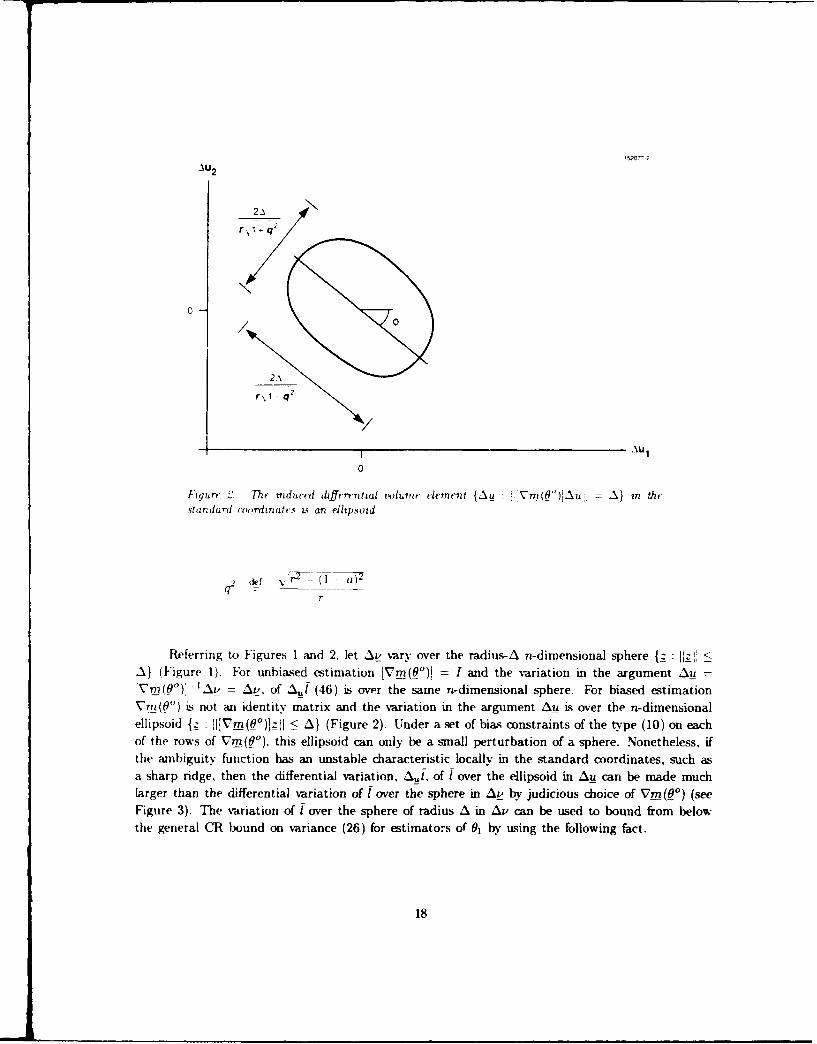
(ellipsoidal) volume element {Au : l[Vm(__)]A: A} in the standard coordinates. Figure 2corresponds to the case

V d. [Ia b]

where a << 1 and b > 0. In Figure 2 the angle of the principal axis can be shown (through

considerable algebra) to be

,P = tan- r( 2 -I- a )2

and the positive parameters r and q2 are given by

clf (I -a)2+b2 + I

2

17

AU 2

r 1 q 2

2A

~H 0r\1 q2

-I Aul

Fgar Thc riduced dzfferential vol)une element {Au Tm(0")iAun = tn tstandan (,ordinatt's u. an elipsoid

def , - (1 aqv_

r

Referring to Figures 1 and 2. let Av vary over the radius-A n-dimensional sphere {z I--' <AJ (Figure 1). For unbiased estimation [Vm( 0 °)I = I and the variation in the argument Au =TVm(O)lAv = AV, of Au[ (46) is over the same n-dimensional sphere. For biased estimationVm(0 ° ) is not an identity matrix and the variation in the argument Au is over the n-dimensionalellipsoid {z : J[Vm(_0 )]_zJl !_ A) (Figure 2). Under a set of bias constraints of the type (10) on eachof the rows of Vrm(e), this ellipsoid can only be a small perturbation of a sphere. Nonetheless, ifthe ambiguity function has an unstable characteristic locally in the standard coordinates, such asa sharp ridge, then the differential variation, AJ1, of 1 over the ellipsoid in Atu can be made muchlarger than the differential variation of ! over the sphere in Av by judicious choice of Vm (e') (seeFigure 3). The variation of I over the sphere of radius A in At, can be used to bound from belowthe general CR bound on variance (26) for estimators of 01 by using the following fact.

18

.12

02

Figuf S. The constant contours of a hypothetical ambiguity function 1(u_, 0 ), over u E Efor fixed 0 = 09, and the superimposed induced differential volume elements of Figures Iand 2. Because the ellipsotdal region includes a greater number of contour hnes, themaximum varatton of over the ellipsoidal rmgion is greater than the variation over thespherical region.

19

FA -:

A 2

B6, >y[ max f (47)2 IlAV12 <A2

where Bb, is the CR bound (28) and ( is o(IIAvlI 2 ) o(A2).

Hence, if the variation of 1 is small, i.e, [ has a broad peak, in the transformed coordinates.,then (47) asserts that Bb, must be large, implying poor variance performance of estimators of 01with mean gradient matrix Vrn(f). More important, if a bias-induced coordinate transformation onthe search parameter Av = [Vm(O)]Au can be found for which the local variation of the ambiguityfunction over the ellipsoid {Au : I[Vm(q)bAuI <_ A} is large, then a reduction in the CR boundmay be possible.

Proof of Fact. Fix a parameter value 0. Define Av:

FAV b ' (48)

where Fb 2 is a square-root factor of the (positive-definite) matrix F - ' [see (24)].

It is shown that Av (48) is a vector contained in the radius-A sphere {z : II <A}, becausethe norm squared of AV is

IIAV112 f, Fb Fb IelA 2

- F -e f-l A 2 =A 2 (49)

Furthermore. substituting Av F A ;nto (42) and (44), nil has the form

1(0 + [V (9)Av - ) TFbV + O(A 2 )

20

= 1 Fb e1 ]T[ Fb A]

A 2 e2eA2 1 1

b- b -,N(+ A)

2 eTF-l + °(A) (50)-1 b e

Now (50) gives the value for A,, evaluated at a point Av (48) contained in the radius-A sphere.Hence, the maximum magnitude of A,) over the radius-A sphere must be at least as great as themagnitude of the right-hand side of (50). This, and the elementary inequality Ix - Yj ? lxi - lyl,gives the bound

A2 1 _ ( 2max AJI > - + 0(A 2 ) (51)

IAL12<A2 2 Bb,(0)

Multiplying this inequality through by Bb / maxlA. 112 <A lAI gives the statement of the fact (47).

21

5. A NEW CR BOUND FOR ESSENTIALLY UNBIASED ESTIMATORS

Here we obtain a new lower bound which is applicable for essentially unbiased estimators,i.e., those whose bias gradient is small. Assume that the bias b, is such that IIVb1(_)I2 < 62 for all0 E e. The starting point for the lower bound is the obvious inequality [see (28)]

varo(1) > Bb, (_) > min Bb, m() rin [feI + d]TF-[e1 + ._ (52)S:llV 9b1 II2 <62 d:Jldll2 <62

This gives the lower bound valid for estimators b, which satisfy the bias-gradient constraint (10)

vare(OI) > B(0,6) , (53)

where

B(,6) d min [ei+4]TF-lki+d] (54)d:l1dll2 <62 -

Note that by definition B(0,0) is just the unbiased CR bound. The bound (53) is independent ofthe particular bias, bl, of the estimator as long as the bias constraint is satisfied. The normalizeddifference

B(_0,0) - B(0,6)AB(O,6) = - B(6,) (55)

is the potential improvement achievable over an absolutely utbiased estimator, i.e., AB(-,b) mea-sures the bias sensitivity of the unbiased CR bound. The sensitivity is a real number between 0and 1, and increased sensitivity corresponds to a larger difference.

The new bound is specified by the solution of the minimization problem (54). We find thesolution in the following theorem and corollary.

Theorem 1 Let 61 be an essentially unbiased estimator of 01 with bias b1 (6) which satisfies theconstraint (10) IVb l [12 < 62 < 1. The lower bound B(2,6) (53) is equal to

B(0,6) = B(6,0) - A62 - eT[I + A]F_1 , (56)

where \ is given by the unique non-negative solution of the following equation involving the mono-tone decreasing convex function g(A) E 10, 1]:

23

g(,) tf _T[I + AF]-2Xel = 62, A > 0 (57)

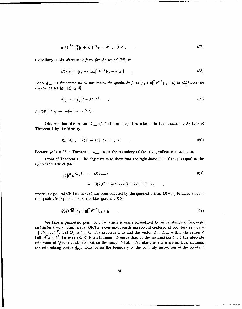
Corollary 1 An alternative form for the bound (56) is

B(e,5) = [feI + dn jTF-l[e +. , (58)

where d,,n is the vector which minimizes the quadratic form ie + d]T Fl [ + ] in (54) over the

constraint set {4: I1dl < 6}

dT = eT[I + AX]- 1 (59)

In (59), A is the solution to (57).

Observe that the vector drain (59) of Corollary 1 is related to the function g(A) (57) of

Theorem 1 by the identity

er[1 + \]-2e,(0

d- n e[ + XF]2n = g(\) (60)

Because g(A) - 2 in Theorem 1, dr is on the boundary of the bias-gradient constraint set.

Proof of Theorem 1. The objective is to show that the right-hand side of (54) is equal to theright-hand side of (56):

nin Q(d) = Q(dn.u) (61)d:1d 112 <62

= B(_,0) - A 2 - eT[I F-_e

where the general CR bound (28) has been denoted by the quadratic form Q(Vbl) to make evidentthe quadratic dependence on the bias gradient VbI

Q(d) [e + d]T F-'[ 1 + d] (62)

We take a geometric point of view which is easily formalized by using standard Lagrange

multiplier theory. Specifically, Q(d) is a convex-upwards paraboloid centered at coordinates -e =

-[1,0,... , 0 ]T, and Q(-el) = 0. The problem is to find the vector d = drain within the radius 6ball, dTd < b2, for which Q(4) is a minimum. Observe that by the assumption 6 < 1 the absoluteminimum of Q is not attained within the radius 6 bal. Therefore, as there are no local minima,the minimizing vector d n must be on the boundary of the ball. By inspection of the constant

24

contours of Q(d) (Figure 4), the minimum is attained when the contour of Q(d) is tangent to theboundary of the radius 6 ball, i.e., the gradients are collinear and of opposite sign;

VdQ(d) = -AVd dTd (63)

for some A > 0. Using the rules of vector differentiation for quadratic forms, (4) and (5), (63) isequivalent to

F- _ + _d] -Ad (64)

152077-4

d2

id

Figure 4. Plot of the constant contours of Q(d) and the domain of the constraint d Td <62. The minimum of Q is achieved at the point indicated by the vector d_.im which isnormal to the tangent plane between Q(d) and drd = 62.

25

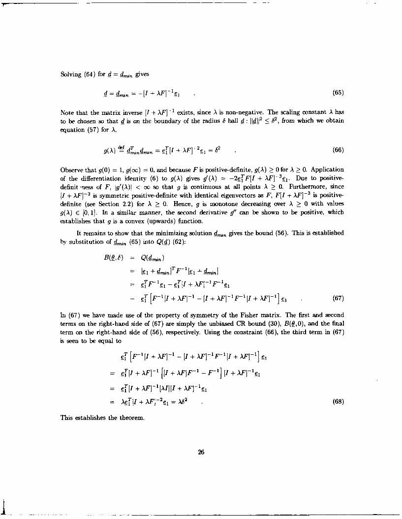
Solving (64) for d - _d,, gives

d = _ -[I + XF]-' _ (65)

Note that the matrix inverse [I + AF] - ' exists, since A is non-negative. The scaling constant A has

to be chosen so that d is on the boundary of the radius 6 ball d: ]jd12 < b2, from which we obtain

equation (57) for A,

g(\) rid= _ = eT[I + XF]-2C1 = 62 (66)

Observe that g(0) = 1, g(oc) = 0, and because F is positive-definite, g(A) > 0 for A _> 0. Application

of the differentiation identity (6) to g(A) gives g'(A) = -2eTF[I + AF]-el. Due to positive-

definit ness of F, Ig'(A)] < oc so that g is continuous at all points A > 0. Furthermore, since

[I + AF]- 3 is symmetric positive-definite with identical eigenvectors as F, F[I + XF]- 3 is positive-

definite (see Section 2.2) for X > 0. Hence, g is monotone decreasing over A > 0 with values

g(A) E [0, 1]. In a similar manner, the second derivative g" can be shown to be positive, which

establishes that g is a convex (upwards) function.

It remains to show that the minimizing solution d,,i,, gives the bound (56). This is establishedby substitution of dMM (65) into Q(d) (62):

B(_,6) -

- e 1 +d iFF-F +n

i _eT-ll, _IT(I + \kF]-'F-'~e,

- T [F-'[1 + AF'-_ [I + XF]-' F-I + 1+ k - 1 . (67)

In (67) we have made use of the property of symmetry of the Fisher matrix. The first and second

terms on the right-hand side of (67) are simply the unbiased CR bound (30), B(6,0), and the final

term on the right-hand side of (56), respectively. Using the constraint (66), the third term in (67)

is seen to be equal to

_T [F-1Il + >FI 1 - [I + AF]-'F-' [I + AF- _el

= 11 + AF1- [11 + AF -1 - F-'] [I +,A]-le I

= _ + XF- 1 [AI][I+ XF-ll

= \e r[I + XF]- 2 el = \6 2 (68)

This establishes the theorem.

26

L ...

As stated, Theorem 1 gives a bound B(9,6) for which the (1,1) element of the inversesof the n x n matrices F[I + AF] and [I + AF]2 must be computed. These calculations can beimplemented by sequential partitioning [9]. A more explicit version of B(6, 6) will be of interest forthe approximations of Section 6.

Let the Fisher information matrix F (21) have the partition

F = a (69)c F,

where a is a scalar, c is a (n - 1) x 1 vector, and F is a (n - 1) x (n - 1) submatrix. Define the

inverse matrices

F [ (70)

(I + X 1 (71)2 J\ V\]

Using the partitioned-matrix inverse identity (2), a, a\, r, f, and O have the following expressionsin terms of the elements of F (69):

a = (a - cTF-lc)- (72)

0 = -aF ,-c

F = F- 1 + aF,-1 ccT F- 1

0A = (1 + Aa - A2 cT[I + A 8 ]-c) (73)

1 = -AaA[I + F 8 I-c

The quantity rA will not be explicitly needed and is omitted.

In (69), c represents the information coupling between estimates of 01 and estimates of theother parameters 02,... 0,. This can be seen from the fact that for unbiased estimation the CRbound on 01 (30) is (F - 1 )11 = a = (a - cTF,-lc)- , which is identical to a-1 in the case c = 0.

27

Theorem 2 In terms of the partitioned Fisher information matrix (69), the bound B(O, 6) and the

associated constraint equation (57) of Theorem 1 have the expressions

B(_,b) = B(_,O) - Ab2 O Taa - (74)

and A is the unique positive solution of

1 + A2cT[I + AF]- 2 C_g(A) = (1 + Aa - A2CT[I + AF,]-Ic) 2

Furthermore, the minimizing vector (65) of Corollary 1 is given by

_dnn=[_a,, __T]T = a,\[-1, Ac'P[I + )Y8]-I]T (76)

In (74), (75), and (76) a, a,\, 3, and 0-\ are the quantities given in (72) and (73).

Proof of Theorem. Substitution of the inverses F- 1 (70) and [I + AF]- 1 (71) into the expressionsfor B(6,b) (56) of Theorem 1 gives

B(9,)_ -_A62 -e1 f

- B(,o) - -[a,3 T]T

= B(_,0) - A62 - aa -33 , (77)

which is expression (74). Similarly, substitution of (71) into the expression for dn (65) of Corol-lary 1 gives

-[I + F I

L rA _AC=,\[-1, AcT[I + XF1]-I]T , (78)

where, in the last line, the identity for --- (73) has been used.

Squaring the matrix [I + AF] - ' (71), we find that the constraint equation (57) of Theorem 1has the following expression:

28

.. ....! .. .. ..

g(A fTI -2 =a2 T, b 2

AF] + 3_3 (79)

Application of the identities (73) to the previous equation gives the equivalent expression for g,

g(A) = + A\_ T[I + AF ]-2 c (80)

= 02[1 + A2 cTI + AF] 2 £]

1 + A2 eT[I + AFs]-2C

(1 + Aa - A2CT[I + \F,]-IC) 2

which is equivalent to the expression in (75). This completes the proof of Theorem 2.

The bound in Theorem 2 does not have an analytic form in general because the solution A to(75) is not given explicitly. Numerical polynomial root-finding techniques can be used to solve (75),or equivalently (57), for A. In particular, as the Fisher matrix F, is positive-definite and symmetricit has the representation F, = Q4pQT, where Q is an orthogonal matrix with columns q, and 4) isa diagonal matrix with diagonal elements Oi > 0, i = 1 . . Hence, we have

E[ + AF] 2 e = I + AQ4QT] 2e (81)

= £T (QOi + A4)IQT)-2ce

j Q[I + A4I- 2QT1

1 (LTq,)2

Therefore, inserting the expression into the left-hand side of (57) and multiplying both sides byHi= 1 [1 + Aoi]2 , we obtain a polynomial equation for A:

Tq) 2 ]JT + Ao,1- + ]2 2(82)i~ 1+ Aoij t%)11+AO [+ o]

3=1 3=1

-i[1 + Oj A 2 (ETq 2 = 62 171[1 + A,, 1i=1 3i j=1

Subtraction of the right-hand side of (82) from the left-hand side gives a polynomial in A of degree2n which must be set to zero.

For the special case of zero information coupling, c = 0, an explicit expression for A can befound and the bound B(0,6) of Theorem 2 has an explicit form. From the definitions of 0, a,, _

and 0,\ (72) and (73), c = Q implies that o = a - ' = B(6,0), cv,\ = (1 + Aa) - ', and = = O.Furthermore, from (75)

29

b2 = =(83)g. =(1 + Aa)2 I

and, consequently,

A = a-1 (6- - 1) (84)

Hence, using (83) in (76)

d -[-C 0 T]T = [-,-OT]T _ b, (85)

and, from (58), the bound is

B([!L) = [e_ 4 dmrF-'[l + dd] (86)

= [- 6e1 rTF-[E - 6 1 ] = (1 - 6) 2eTF-e_

= (1 -6) 2 B(,0)=(1 -6) 2a- '

Observe that zero information coupling implies two important facts: small bias gradients havevery little effect on the general CR bound, as the difference (55) AB(O,b) = 1 - (1 - 6)2 Z 0; andcoupling of the bias, b,, of 9j to the other parameters 02, •. 8,0 is not likely to significantly reducethe CR bound, as the CR bound's minimizing vector d,j, (85) makes the bias of j, independentof the other parameters.

In the following sections we will assume that c $ 0.

30

6. A BIAS-SENSITIVITY INDEX AND A SMALL-6 APPROXIMATION

In the previous section the form of a CR-type bound B(6.6) was given in terms of an un-determined multiplier A given by the solution of 9(A) = 6'2 (75). For the case of zero informationcoupling, g(A) has a simple form, giving an explicit solution for A and B(_,6) (86). Otherwise, anexact analytic form for B(0.6) is difficult to obtain and the solution A to (75) might, for example,be calculated using numerical polynomial root-finding techniques applied to (82). In this sectionan o(b) approximation is developed for B(_, 6) which converges to the true solution as 6 approacheszero. Associated with the approximation is an approximate minimizing bias-gradient vector _,i,,which achieves the o(6) approximation to B(_, 6).

While the approximations offer little computational advantage relative to the implementa-tion of the exact computation indicated in Theorems 1 and 2, the approximate analytical formsprovide some insight into the important factors underlying the bias sensitivity of the CR bound.In particular, the bias sensitivity of the CR bound is characterized by the slope of B(_, 6), at6 = 0. A large slope implies that a small amount of bias can substantially decrease the nominallyunbiased CR bound, corresponding to high sensitivity. In the sequel, this slope will be related toa bias-sensitivity index.

For convenience, formula (75) is repeated here:

'(A) = I + A2cT[I + AF]-2 c =(1 + Aa - A2cT[I + AF,]-1) 2

The idea behind the derivation of the o(6) approximation follows. Theorem 1 established that g(A)is convex and monotone decreasing over A > 0, g(0) = I and g(oo) = 0. Therefore, tor a sufficientlysmall value of 6, the solution A to g(A) = 62 is sufficiently large so that simultaneously

A£T[I +AFs]-1 £rF1c and A2 T[I +AFs 2 c cTF- 2c (88)

If (88) holds, the constraint to be satisfied (87) becomes the simpler equation

1+ cfTF -2c = 2 (89)

(1 +[a - CTF'c])2

from which the solution A is simply computed by taking the square root of both sides of (89) andsolving for A. This solution can be plugged back into (65) and (56) to obtain approximations todmin and B(O.6).

The following proposition puts precise asymptotic conditions on the solution to the constraintequation (87) to guarantee the validity of the approximation (89).

31

Proposition 2 Let A* be given by the non-negative solution of (89)

1 + CT-21C\A~ [a - ,T~l~ , (90)

and assume c $ .Corresponding to A*, define the vector d'ra

With these definitions, A* approximates the actual solution A of g(A) =62 A > 0 (75), in thesense that

1. 0 < g(A*) 62, so that d' does not violate the cornstraint (10) on the bias gradient.(Recall, from (60), that g(A*) = lldid 112.)

As a consequence of 2., A6 = 0(1) and also -1 = 0(b).

To prove Proposition 2 we will use the following:

Lemma 1 Let c - Q and define the positive quantity q;

r TF-lC _.Tr-27q~nn j TF5-2c'C T 3 (92

Then \q -o 0 as 6 ,f 0. Flirthermore, the following bounds are valid for all A > 0:

JFc -F1 (I _ AJ ! C[I + AF8 V'l < cT1 FIC ,(3

C l _ 2 2 \ 2 C [I + AF 8 V-C < CT F-2 C .(94)

A weaker set of bounds is obtained by replacement of q in (93) and (94) by the minimum eigenvalueA , of the matrix F,. Flurthermore, from (93) and (94), ACT[I + AF,]-1 c = cTF,-lc + 0(1) andA 2CTfI + AF.J-2 C = CT F 2 C + 0

32

Proof of Lemma 1. Recall from Theorem I that g is a continuous, monotonically decreasingfunction with limy-.. g(A) = 0. This implies that the inverse function g-1 is continuous monoton-ically decreasing with lini,,-og-'() = oc: therefore, if q is fixed and nonzero, for sufficiently small6 the quantity Aq can be made arbitrarily large. Hence, Aq - oc as 6 - 0 as claimed.

The right-hand inequalities in (9:3) and (9-1) follow from the inequality for a positive-definitematrix A and arbitrary vector x:

XT[I + A]-*, < .'T:I-kX (95)

for any integer k > 0. This can be proven via an eigen-decomposition of A. The left-hand inequal-ities in (93) and (94) are established by application of the Sherman-Morrison-Woodbury identity[Equation (3)];

[I + AF,] - ' F[I, IF'A A As A 3

- - [I + AF]' (96)

Application of (95) and (96) to £T[I + AF,]-'c gives directly

ACrT[I + AF -'c =cTFlc I cT[I + AFs-I'F21c

= - - [I + AF3]-'Fs-[c

> CFsl- I cTF2

= ATF -I£(I - T(97)

Application of (95) and (96) to cT[1 + AFs]-2g yields

A2cr[I+ AF,]- 2 A 2 [I + AFr]-'[I + AFsl-lcA2T1Fs- - A [I + AF. F.,-'][ F3 .AI + AF.h-F] _

= FT F 2 C - 2 £T[I + AF] - ' F 2 c + £T[I + AF]- 2 F[-2 c

> CTF 2- 2CT[I + AFs]-'Fs2c

= CTF' 2 c 2cTF,-'[I + AF,]-'F,'c

> CTF-2C -2 TF'-3

33

7'F-v2_ (1 2-CTF (98)

In obtaining the inequalities (97) and (98) we have used the fact that [I + AF] - 1 , F-', and F 2

are positive-definite matrices with identical eigen-decompositions; hence (see Section 2.2), theseeTF- 2c

matrices commute and [I + AFI- 2 F 2 is positive-definite. By the definition (92), 1/q > C1-

and 1 q > T , so that the right-hand sides of the inequalities (97) and (98) are underbounded

by the right-hand sides of the inequalities (93) and (94) in the statement of the lemma.

Recall the -variational inequality ([31, Theorem 4.2.2) for any compatible vector z and sym-

metric matrix A:

:Tz > , (99)

where A,n, is the minimum eigenvalue of A. Apply (99) to the lower inequality in (97) along with

the definition z dI F-Xc:

T F C (1 1 CTF,- TF -l Z_

>c r, _(1 3 oo

Likewise, the definition z = F- 2c and (98) give

2TF2 K-TFs 3C) T-Fc (1 2 Z)

1 A2 C C

> feTF- 2(- A2 )(1)

This Eftablishes the lemma.

Proof of Proposition 2. Application of the inequalities in the lemma to the expression for

g(A) (87):

g(A) = - (102)(1 + Aa - A2cT[I + XAF cj1 )2

evaluated at A = A* gives

34

I + cTF-2C( I - 2(AqY-') K (A) 1(1~ + 2~ <T~ 1(' < ,q')] [1 + A(a - cTF3-IC)]2

- ~(103)

The right-hand inequality in (103) establishes statement 1. in the statement of the proposition:

g(A*) < 62 .Because the lower bound in ( 103) approaches the uipper bound 62 in (103) as Aq - 00.

g(A') is forced to 62 as A'q - cr- or equivalently. by the definition of A' (90), as 6 -0. To

establish statement 2., recall that g(A) =6(7)and consider the following:

Ab = A V/g (A) (104)

=AV [( _I+ _A2fT[I+ ATFf2

(+ Aa -A2rTjI + AF5])-1 c)2

VI + A2f[I + AF.,1-2c1 -A[I + AF -Ic

Now, by Lemmna 1, (10-4) becomes

A6 71CTS OA)a - J'F-'c + 0( +

-+0O(-) (105)a A

Because A -x as O 0 and~ identifYing n (72), we obtain the limit

limt A ckv I + C 'I C (106)

That lim,...O A6b is identically the righit-hand side of (106) follows directly from the form of A* (90)and the identity (72).

We next derive an exp~licit expression for the slope of B(6. 6) (56) at 6 0. This expressionwill be used to develop an o(6) appr-oximiation to B(9.6).

Theorem 3 Thf derivatives of the bound B(eJ ) and of the normalized difference between the

unbiased CR bound and this bound. _NB6 ) = (e~o) ,&6 exist and are given by

dBq.b -2B(6.0)F an 1 2 ~ (~~ 6=o = 2 1 + i' 2 (107)

:1.5

where 77 is the bias-sensitivity index defined by

2) def

77= IIF8'-Il11 = CT F - 2 C (108)

Proof of Theorem 3. The existenc.e of the derivatives will follow from the existence of limb- 0 6which is derived in the following expressions.

For convenience we repeat (74):

B(e, 6) = B(O, 0) - A6 O- na (109)

where

a =(a - cTF-jc)1 = B(q,O) (110)

and

Ct (1 + Aa - A 2CT [I + XFJf'cf'I (111)

3A -AaA\[I±AF.J'c

The use of the identities for a, a,\, fi, and fl,(110) and (111), gives the following equationfor the difference B(6,0) - B(0,6):

B(9,0) -B(0,6) = A6 2 +±ka + ,L3 (112)

= A62 + o,\ ra+Aa,\f T [I +A;]X F. 1 'ca

- At + a(1 + \AT[I + X F-'7c) a,] 6

so that

B(6,0) - B(9,b) - 6+(+A JX]1 1C) 2 (13

Next we develop the following facts:

e Rohm (93) of Lemma 1 and the forms of a, (111) and a (110),a,\ _ 1 1\(114)

6 - 1±A -A2CT I±F.]c G)

36

1 + A(a -cTF-1c) + .0(l) (6)

I+ -A+ 0(1)

- + 0(b)

A completely analogous argument as used in proving (93) of Lemma 1 establishes

AcT[I+AF]I-lFIc = cTF-2C+O()

= cTF+- c - 0(6) (115)

Substitute relations (114) and (115) into the right-hand side of (113) to obtain

B(e,O) - B(9,6) (116)

6

= A6 l+cTF2c + O(6) A-+(6)

Recalling the result of Proposition 2,

Ab -- aq1 +cTF 2c , as 6--0 , (117)

take the limit of (116) as 6 -, 0 to obtain

dB(, 6) = =lim B(0, 0) - B(0,6)

db 6-0 6

= a 1+ cTF- 2c + a(1 + cTF-2C),

= 2a + TF 2 c (118)

Because a = B(,0), the first identity of (107) is established. The additional observation that

d=B(0,6) dfB(9,o)-B(0,6) = dB(,6) 1db B(0, 0) j d6 B(0_,0)(19

establishes Theorem 3.

37

T'heorem 3 can be used to approximate the form of the bound B(6, 6) up to o(6) accuracy; in

particular, B(6,6) B(6,0) + 6 dB(QI) 16=o for sufficiently small 6. We have the following:

Theorem 4 The lower bound B(Q,b) (56) on the variance of 61 has the representation

B(O, 6) = B* (9,6) +o(6) ,(120)

where

B'(O,6) B(,O) (1 -26V 1cTF;) (121)

Define the vector d; ,.

d~ru. = 6 F- (122)

zs an o(b) approximation to the minimizing vector of B(O,b) in the sense that

[fl + dZ.TFl 1 ~ =* B(O.6) + o(6) .(123)

Proof of Theorem 4. The relation (120) is just a consequence of the form of the derivative (107) ofB(O .6) at 6 =0, given in Theorem 3, and the Taylor expansion

B(O, 6) = B( ,O0) + 6dB (,6) 16 =0 + O6) (124)db

= B(q,0) -2B(V,0)6 1 +cT'+ o,(b)

To establish the second part of the theorem, (123) must be shown to hold. For notationalconvenience, define

def 6 (125)

38

so that d = oj-lcTF,-l]T . The substitution of d**. into the left-hand side of (123) and

identification of the inverse Fisher matrix (70) gives

[I +d** ]T F- 1 + ** (126)

[1 aa,,a.ocTF4 ][ a aT]aCTFl]T3r

a.(1_ )2 a+2 ao(1 0a)J2F,-' c+c FFr

Now recall the definitions (72) for a, 0 and F:

a = (a - cTl<c)- 1 = B(,0) (127)

4 = -aF.'c

r = + aF-Icc T F 1

Substitution of (127) into (126) gives

[g, + d*IT F -1 [e, + d,.] (128)

= a(1 - aoc) 2 - 2aa..(1 - aoo)cTF -2c

+a cT F-[F + aF- cc T F,-F-lc

= a[(1 - 0.) 2 - 2-2(1 - TF)F2 + -(cTF;72 c)2 ]

+a 2_CT F-3 C

= a[l - a. _ -cTF-2C 2 + a2CTF - 3c

= a[1 - a"(1 + CTF;-2 C)]2 + a2 _TF-3

Finally, recalling the definition (125) of ao,

[_tl + d*. n]T F - 1 I + d d n] (129)

6 + cTF-2C)]2 +62 cTF 3 c= [I - c1+cTF-2c

cT ~ 1+cF 2

= B(0,0)[1 - 6V1 +cTF- 2C12 + o(6)

= B'(,6) + o(6)

= B(_,6) + o(6)

39

where in (129) we have used the facts a = B(6.0) (70), and B(6, 6) = B'(2,b) + o(6) (120). Thisfinishes the proof.

The following corollary to Theorem 4 will be needed for the sequel.

Corollary 2 If for a given point 0' the Fisher matrix F(O) is invertible at 9 = 90 and its elementsare uniformly continuous over an open neighborhood U of 9O

, then an open neighborhood V C U of90 exists such that in (120) lo(b) converges to zero uniformly over ( E V as b - 0.

Proof of Corollary 2. Denote by HJAIl the norm of the square matrix A ([3], Section 5.6) and defineE(_) = F(6) - F(O° ). Because the elements of F(6) are uniformly continuous over a neighborhoodU of g0, IIE(_)f converges uniformly to zero as 0 - 90, and since F(2_) is invertible, an openneighborhood IV1 C U of 0' exists such that F(6) = F(6_° )+ E(0) is invertible over 0 E W. Therefore,using the inequality IIF-'(0) - F-( 0 )ll < IIF- 1 (_)11 -. IF-'( 0 )jj IIE(7)II ([3], p. 341, Exercise 13)F-1(2) converges to F-1(6') uniformly over the neighborhood It" of 90. Hence, F(_) and F-'(g)are both uniformly continuous over the neighborhood W of 0. Now recall the definition (57) ofthe function g(A) = go(A): go(A) Lef e[I + AF(0)J2ej. Since I + AF(_) is invertible and uniformlycontinuous over the neighborhood U of 90, a similar argument establishes that g(A) is uniformlycontinuous in 0 over a neighborhood 1V of 00, where without loss of generality we can take W' = W.It can also be verified that for all 6 > 0 the function B'(7,6) (121) is uniformly continuous in 9over the neighborhood HW of 0' . Define f(_ A) = go(A)- 62 where _ef [6, OT]T. From the uniformcontinuity of g_(A) it follows that f(_, A) is uniformly continuous in _ E IR+ x IV. Furthermore,applying the identity (6) to f(, A), the derivative Vof( ,A) = -2eTF(()[I+ AF(()]-3 e is nonzeroand continuous in A for A > 0. Define _ = 6,0T] . By Theorem 1, for any 6 > 0 a unique pointA' exists such that f( 0 , A') = 0. We can now apply the implicit function theorem ([10], Chapter4, Theorem 15.1) to assert that an open neighborhood I C U' exists such that the solutionA = T(6,8) to the equation g_(A) = 62 is uniformly continuous in 8 over 9 E V. Therefore, inview of the functional form (56), the bound B(_,6) is uniformly continuous in 0 over 0 E V. Theremainder term o(b) in (120) is thus equal to the difference B(0,6) - B*((,6) of two uniformlycontinuous functions; therefore lo(b) converges to zero uniformly over 0 E V. This establishes thecorollary.

40

7. DISCUSSION

In this section issues related to the bound of Theorems 1 and 2 will be briefly discussed.Some general issues are of importance: Is the bound of Theorem 1 achievable with any practicalestimator? What does the bound (56) imply about the inherent performance limitations of unbiasedestimators in the presence of nuisance parameters?

7.1 Achievability of New Bound

If for all 0 in a region D C ( an unbiased estimator achieves the (unbiased) CR bound,B(0,0), on MSE (recall that MSE equals variance for unbiased estimators), then the estimator iscalled efficient over the region. An estimator that by virtue of its bias has MSE which is less than orequal to B(6,0) for all 0 in a regic l D C E, and strictly less than B(6,0) for at least one 0 E D, iscalled superefficient over D. Assume that D is a finite rectangular region D = D1 x-.- x D,, whereDk is an open interval, k = 1,... ,n, and also assume that F(e) satisfies the uniform continuityproperties over U = D assumed in the Corollary to Theorem 4. While achievement of the boundB(6, 6) is not necessary for superefficiency, if for a sufficiently small value of 6 (to be specifiedbelow) the variance of an essentially unbiased estimator 01 achieves B(6,6) for all 0 in an openregion D, then an open region V C D exists such that 01 is a superefficient estimator over 0 E V.To be specific, because the bias gradient of 01 satisfies the condition (10), for all 0,0' E D

Ibl (_) - b1 (#')I

lb Ib(_) - bl 18, 02,.. ,S) + bl (00, 02,... ,0n) - bl (tr,802,...- , 0.)

+bl (00, 0 ,. ..... ,O,,) ... .b( , , 0, _1 , 0,.) + bi (00,. -.. , 0.0_-1,0,,) -bi (00)

< lb , (_ ) - bl (01,02,.. ,O- 00 + lb (0 , 02,...- ,0 .) - b l (0 ,02,...- ,O,0 )1

+ -.. + lbl (00,. .0.,0,-1,0.) - bl (e°)l

+ - -1 + &U du 2

n

< 6 max IO, - P I- = D,

= 6M , (130)

41

ITwhere M is a positive constant independent of specific values -0,0° E D:

M2 'max 10i - Oj- (131)D9,

As D is finite, maxD, 1 0i - 61il < 00 and M is finite. Assume without loss of generality that a point00 E D exists such that b (0o) = 0 (if no such point exists, pick an arbitrary go E D and redefine

01 to be 01 - b (- 0)) Assume vare(0 1 ) = B(6, 6) for all 0 E D. While it follows from Theorem 2that for any b > 0, B(-,6) < B(6,0), V, we need to show that MSEo(OI) :_ B(9,0), where strictinequality holds for at least one point 0. The form (120) of B(#, 6) in Theorem 4 gives for all 0 E D

AISEo(01 ) = B(-, 6) + bq(6) (132)= B(,O)1-2b 1 + CTF2c) + o(b) + b(0)

Therefore, subtracting B(,0) from both sides of (132) and using the bound (130),

AISE( - B(-,0) = -6[2B(-,0) V1 -cTF- 2c o(6)] + b() (133)

< -6[2B(9,0)/1 + cTF;2 c_- o(6)] +

= -6[2B(0,O)/1 + TF8 -2c- o(6) -M2 ]

Now, assuming uniform continuity and invertibility of F(e) over 0 E D, by Corollary 2 a regionV C D exists such that the quantity lo(b) converges to zero uniformly over 0 E V. Hence, since

2B(0, 0)1 + cTF 2 c > 0, a sufficiently small positive 6 exists which is independent of 0, such that

MSEo(0 1) < B(9,0), V-0 E V (134)

Therefore, 01 is a superefficient estimator over V.

The condition that the variance of 01 achieves the variance bound B(0, 6) everywhere in D isunnecessarily restrictive. There are two necessary conditions for the achievability of B(-,6). First,a real bias function b, (-) must exist that has the minimizing vector _drai, (-) as its gradient over D.If di,, is the gradient of bl, the gradient Vo4.,,n is equal to the Hessian matrix of bl (-), whichis always symmetric; therefore, the first necessary condition requires that Voed ,,n be a symmetricmatrix. Second, since B(-, 6) is a CR-type bound, the sufficient condition for equality in the Schwarzinequality underlying the derivation of the CR bound must be satisfied. This latter condition canonly be satisfied in the case of parameter ctimation for exponential families of distributions ([11],

42

Theorem 1, 16], Chapter 1, Section 7). As these two necessary conditions cannot always be satisfied,the variance bound B(6, 6) is generally not achievable over any region D.

If for some point 0 an efficient estimator exists for the vector 0 over an open neighborhoodof 00 , then an essentially unbiased locally superefficient estimator can be constructed. 91 is calledan essentially unbiased locally superefficient estimator at the point 0 if 01 is essentially unbiasedand if MSEoo(b1) < B(9_,O) while MSEe(61) :_ B(6,O) for 0 over an open neighborhood of _0.

Local superefficiency is a weaker property than global superefficiency because a locally superefficientestimator only requires superefficient performance in the neighborhood of a particular point 0' andit may have MSE which exceeds B(6,0) outside this neighborhood.

Let 0" be some fixed point in E and let a 6 > 0 be specified. As in Corollary 2, assumethat F(O) is invertible and that F(P) is uniformly continuous over an open neighborhood U of 0.This assumption implies that an open neighborhood V C U of 0 exists such that F-1 () exists

and is uniformly continuous over V. Now assume that 8ff is an efficient estimator for 0 over the

neighborhood V, i.e., bef is unbiased over V and

ER(e l f __)(_ eff _ O)T] = F-'(_), 8 V (135)

The daim is that the following estimator is essentially unbiased, locally superefficient in an openneighborhood of 0:

81 = + dU. (90)]T( 9 - _00) (136)

where d M.(f) is the vector given in Theorem 1. Because Eo[8_f] = 0_, we have for the bias of 81

bi(6) = E_[61 - 01] (137)

= E[Oo + _1 + d,. (o)]T(oefl -f 0) 0 ]

= 1-i1 + d =.(0)]T(e - -o) - (01 - O )

[-, + di. (-)T(- - o) - fT(# - go)

_dT(_O)(_ - "), VO E V

Hence, the bias gradient Vb1(6") is simply dTn (90), which by Theorem 1 satisfies the constraint

d~ d,,n < 62 and the estimator ii (136) is essentially unbiased over 0 E V. Furthermore, the

MSE of 01 is equal to

MSEo(6 1 ) = E1[(0 1 -01)2]

43

= Ee_[(0± + - (-0)]T(-e 1 f -+ 0) -01)2]

E_[e([, + d_. (00)]T(9e!I -0) - _T[ - Qo1)2]

= E[([el + d ,,.(o)JT( 91

- _0) + _ + d..(0°)]T[ - 90] - e_[_ - _o)2]

- Eo[([e, + _ (90)]T(_e -- _8) + d T .(_0°)[ - 0])2]

= [_ + d. ()]TF-l(8)[e - dT (e0 )] + (dT (0)[ - _0 ])2

- [1e + d,.(o) T F-l(_)[ej + 4,(O)j + b(_), V8 ) V (138)

Define the function e(0)

e(O) f MSE_(O,) - B(9,O) (139)

= (o)+ F-,()°)T F ()[e 1 + .d. (0)] - eTF - 1 (O)feI + b()

Note that when 0 = 00 , MSEoo(9,) = B(6 0 ,6) so that e(0) < 0 for all positive 6. Furthermore,

e(0) is uniformly continuous over 0 E V because F-I(0) is uniformly continuous over 0 E V and

b,(0) (137) is linear. Hence, for any -y > 0 and any 2 E V an E = c(-y) independent of 0 exists suchthat

Ie(o) - e(_O){ < (140)

whenever lie - _0°[ < E(-y). Relation (140) implies

e(0) < e(O°) + -

As e(_0 ) < 0 a -y = -y' exists sufficiently small so that e(_) < 0 for all 0 in the neighborhood 09=Ile - 6

011 < E(y'). Consequently, MSE_(0,) < B(0,0) for all 8 E 0 and 01 is locally superefficient.

7.2 Properties of the New Bound

The behavior of the new bound will be treated by listing some of its properties. For conve-nience we repeat equation (107) for the slope of the difference AB(_,6):

dAB(O, 6) -2d1B(, -0 2/1 _ _ ,C (141)d6 6=o 2 1%cT Fa - c ,(1)

where

44

AB(8,-) = B(O,0) - B(_,6) (142)

B(_,0)

Properties:

1. The slope (141) is positive (because F 2 is positive-definite), as expected becauseB(_, 6) is less than the unbiased CR bound B(Q, 0). More significant is the fact thatto o(6) approximation the relation between B(_,b) and B(_,0) is multiplicative as

a function of b: B(_,6) - B(_,0)(1 - 2V1 +cTF- 2c) (recall Theorem 4). Thisprovides indirect evidence for a potential for severe bias sensitivity of the CR bound.

2. The slope (141) of AB(_, 6) is characterized by the length of the vector F-'c, aquantity which has been identified in Theorem 3 as the sensitivity index n,

dlef c=

77 I F,- 1T 2 cc (143)

77 is a dimensionless quantity which measures the inherent sensitivity of the unbiasedCR bound to bias in the sense that -2v/1 + r? is the per 6 decrease of B(9,6)relative to the unbiased CR bound B(6,0). A useful form for 77 is given in terms ofthe elements of the inverse Fisher matrix F - 1 (70) and (72)

I/-- - (144)0

3. The quantity 7 (143) can be interpreted in terms of the "joint estimability" of theset of parameters 0 = (0 ... ,On)

T by recalling the CR matrix inequality (23) forthe covariance of an unbiased vector estimator 0 = (6,,... ,9,)T,

1 0"12 • " ln

cov_(O) > : F - 1(145)

On 1 Cn2 -"- • n

This gives a correspondence between 77 and the covariance between a set of optimalunbiased estimators, i.e., an efficient estimator eff i = 1,... ,n,

IIc T F'- i 211 012 1- in1 I

= id (146)

where Pij is the correlation coefficient between eif ! and eif;

45

&ef O'ijPd = - (147)Oriol,

In light of (146), the set of important but difficult-to-estimate parameters is of par-ticular significance; these are information-coupled with 01 (Pl, $ 0) but their best

unbiased estimators have large variance (var(je9f) a > 0). (143) is a measureof the propensity of these parameters to influence the estimator of 01.

4. Note that the slope (141) of AB(6._6) is minimized for the case 772 = cT F-2C = 0, as

db 6 = T1 +7 Fs ' > 2 (148)

Therefore, B(_. 6) is the most stable with respect to bias when there is no informationcoupling between 01 and the other parameters so that c = 0 and 7/ = 0. Furthermore,if 772 = CTF,-c = 0. F,-lc must be the zero vector and, from (85), the minimizingbias gradient has the form

d.i" = [-6,0. 0 1T (149)

From the form of the gradient (149) the "best" biased estimator has mean

Eo(0 1 ) = (1 - 6)01 + const (150)

This mean can be obtained by a simple "shrinkage" of an efficient estimator eff, ifsuch exists;

=l =(16)(97" - 0 + . (151)

and as discussed in Section 7.1. 9 is locally superefficient in a neighborhood of _0.

5. Let the Fisher information be such that the ith element of cTF,- l dominates the

other elements: £TF,- [0... 0.(.0 ..... 0]. where as in (146) ( 4'f pliai/al. This

can occur if 0, is a coupled but extreniely hard-to-estimate parameter. Then, thesensitivity index is given by

2 = TF2 (152)77 C F cC Z(12

and, under the additional assumption c >> 1. the minimizing bias gradient (122)takes the approximate form

_L, .= [0. b 0.. 0]T (153)

i.e.,

b()= 6, + const (154)

In this case, a small bias due to information coupling between 01 and 0, can give asubstantial decrease in the general CR bound.

-16

7.3 Practical Implen:ntation of the Bound

From (146), the sensitivity index 77 is apparently dependent on the units used to representthe parameters 02,... , , . For example, if 01 is represented in /rads and 02 is represented in MW,the quantity a2/al in (146) will be much smaller than if 01 is expressed in rads and 62 is expressedin aW. Thus, a parameter may be rendered difficult to estimate solely by virtue of the choice ofunits used to represent the parameter. The choice of units is equivalent to the specification of acoordinate system to represent the parameters (see Section 3). This unit dependency is due to thefact that when taken alone the constraint on the bias gradient is not tied to a particular choiceof coordinates for e and therefore does not adequately describe a user constraint on the bias.In order to use the results of this report, the coordinates for E must be specified, e.g., throughthe specification of a constraint ellipsoid (11) in E over which the bias b(_) is allowed to varyby at most -y. This bias constraint (11) will naturally reflect the user's choice of units for theparameters. In Section 3 we transformed the user's units to make the constraint ellipsoid a sphere(12). The results derived in Sections 5 and 6 are valid in these transformed coordinates. Thereason that we chose to work with spherical constraint regions is that for a nonspherical regionwe could not have simultaneously achieved properties 1. and 2. of Proposition 1 for our form ofbias-gradient constraint (10). Thus, expression of the bias gradient in a transformation-inducedspherical-constraint region guarantees maximal bound reduction, i.e., the greatest freedom on thevalue of Vml (0) subject to the requirement (11), as compared with any other choice of coordinates.

47

8. APPLICATIONS

In this sectioi we apply the previous results to estimation of standard deviation and esti-mation of the correlation coefficient, based on measurements of a correlated pair of lID zero-meanGaussian random sequences. Analytical expressions are given for the unbiased CR bound B(g,O)the sensitivity index ?, and the approxi-nation d' in Theorem 4 for both of these estimationproblems. Then, for the estimation of standard deviation, the exact bound B(_,b) (56) of Theorem1 is numerically evaluated and its behavior is compared to the behavior of the sensitivity index.

Consider the following covariance estimation problem. Available for observation are a pair ofrandom scq _.:ces

1X-\ ', -1 = -\11 .... xi,,,

{X2N,'1I = X 2 1 ..... X2,, (155)

where {[Xh. X 2"]T} are lID Gaussian randomn vectors with mean zero and unknown covariancematrix A;

A a12 ] (156)

Define the correlation coeflicient

df (72 *,-(157)O"1 0"2

where Ol and (7 2 are the positive square roots of (72 and (. respectively.

8.1 Estimation of Standard Deviation

The objective here is to estimate the standard deviation a1 of X 1, under the assumption thata 2 and p are unknown. The likelihood function corresponding to this estimation problem has theform (A.2) from Appendix A

- 2In((2t) 2 a 0 [l - - 21 -r ) 2- +

(158)

1')

where in (158) YX2 is the sample variance of {Xj }:'m= and X1 X 2 is the sample covariance between{X, 1 } and {Xi2} for known mean zero. The Fisher information matrix for a,, a2, and p is derivedin Appendix A, Equation (A.11)

_2 l a2 01

__2 2 (159)(7 - --- 2 C 2_ _ _P +_

01 0"2 1-p 2

In the notation of (7), identify the parameter vector 9:01 9--f aI, 9 def o,2 , and 93 4 p. Theunbiased CR bound B(6,0) (30), the sensitivity index 77 (143), and the o(b) approximation d*.(122) are derived in Appendix A, Equations (A.24), (A.25), and (A.26), respectively,

B(-,o)= 1 , (160)- 2m

"" 1 1, 2 ,+ -P (1 P2) (162)

! ,nzn -= ,71 0"1-Ol Ol 12

The following comments are of interest:

1. The CR bound B(9,0) (160) on the variance of an unbiased estimator &I is function-ally independent of the variance o2 of X2j and of the correlation p between XAi andX2i.

2. If p = 0, then ir= 0, and the general CR bound is minimally sensitive to bias-gradientlength 6.

3. The squared sensitivity r/? (161) is the convex combination of two terms: p andS .Since n2 is inversely proportional to o- , the sensitivity of the CR bound to

small bias can be significant when 2 is small.

4. For p2 dose to 0, the ratio of the first and second terms of (161) is approximatelya2p 2 . In this case, if a2 > the first term dominates ?, while if a2 < 1 the

second term dominates. For p2 close to 1, the ratio of the first to second term isapproximately 2 /(1 - p2)2. In this case, if o2 > (1 - p2)2 the first term dominates,

50

while if a2 < (1 - p2 )2 the second term dominates. In any case, it is seen that o2 1

brings about a much higher sensitivity index than o-2 < 1, particularly for p2 > 0.

A related problem is the estimation of the correlation coefficient p for the above pair ofGaussian measurements.

8.2 Estimation of Correlation Coefficient

clef cef defConsider the estimation of 01 = p, when 02 = a1 and 03 = ca2 are unknown. For this casewe have, from Appendix A, Equations (A.39), (A.40), and (A.41), respectively:

B(e,0) = (1 _ p2)2 , (163)

-2 24 pof= +o 0r2 (164)

2 2(1 - p2)2

d~_ , [_1 ' p p '21T(15-__ = 1 K 2 (1 - p2) l '

2 (1 -p2)a2 (165)

We make the following comments concerning the problem of estimation of p:

1. The CR bound B(6,0) (163) on the variance of an unbiased estimator 0 has a formwhich is independent of the standard deviations o and a2 . Hence, the MSE perfor-mance of an unbiased efficient estimator of p is also invariant to these quantities.

2. As occurs in estimation of a,, the case p = 0 corresponds to a CR bound which isminimally sensitive to small biases.

3. The form of the sensitivity index q (164) indicates that the CR bound is sensitive tosmall biases if the average (or1 + a2)/2 is large and if there is significant correlation

I > 0. This, along with the form of dZn (165), suggests that substantial improve-ment in estimator variance may be possible by using an estimator whose bias is notinvariant to the standard deviations a and a2.

8.3 Numerical Evaluations

Surfaces for the normalized difference AB(6,6) (55) and the sensitivity index 77 were generatednumerically for the variance estimation problem of Section 8.1. The matrix F (159) was input to acomputer program which computes AB(6,6) and 77 as the parameter vector 0- (a1 ,a2,p) rangesover the set { } x [0, 10001 x [-1, 11. For this example, 6 was set to 0.001 and m = 1. In Figure 5the quantity AB(_,6) is plotted over (U2,p) and in Figure 6 the sensitivity index is plotted overthe same range of (a2 , p). A comparison between Figures 5 and 6 supports the approximate small

51

AB (0,8)1 52077 5

0.8 •- -,

0.6 -

0.4,

0.2-

0.0p - 4800.0"

o2400.0

200.0 - _0. 81.0

0.0 0.83 0 .6 0 .4 0 . .0 -- . 4 0

Figure 5. The normalized difference A-B(_, 6) plotted as a function of a2 and p for RMSpower estimation. Increasing values of AB(_,6) correspond to increased sensitivity of theCR bound to small bias. Surface is plotted for 6 = 0.001 and ol = 1.0.

6 analysis in Section 8.1, which was based on an investigation of the sensitivity index. Note thatthe region of p for which the bound B(_,b) differs significantly from the unbiased bound becomesincreasingly large as the standard deviation a2 of X2j increases. Further, when p = 0 then 7= 0 in(161), and we see minimal bias sensitivity. In the limit as o2 -- cc the surface AB(_,6) (Figure 5)becomes a deep wedge centered along the line p -= 0; substantial bound reduction is achieved forall nonzero p. Figure 5 indicates that for small a2 the surface AB(6,6) is close to zero for all p.A simple calculation shows that p2 (1 -

2 )2 attains its maximum for p2 = 1/3. Hence, in viewof the expression (161), r/ ./2r + 4/(27at). Thus, for the present example where or = 1.0,

S< a2 + 4/27. Recalling that AB(_,6) ; 6 (- ) = 26V (107), this implies that ittlebound reduction occurs for small a 2 and 6 = 0.001.

52

Ti

00.0 .1127

600.0-

400.0

200.0

0.0

0. 20 0 0. 8 06.040

Figure 6. The bias- sensi tivity index q~ plotted over the same range of the parameters asin Figure 5.

53

9. CONCLUSION

A new lower bound on estimator variance for almost unbiased estimators in the presenceof nuisance parameters has been derived as a function of the Fisher information matrix and theunbiased CR bound. The new bound has the form (56) which involves finding the positive root A ofa convex function (57). The bound (56) is valid over all estimators whose bias gradient has lengthless than or equal to a prespecified constant 6. It reduces to the standard CR bound on unbiasedestimators for 6 = 0. The sensitivity of the general CR bound to small bias has been characterizedby the slope of the normalized difference between the new bound and the CR bound. This slope ismonotone in a sensitivity index q7 (108). The form of the sensitivity index indicates that the newbound is significantly less than the unbiased CR bound when important but difficult-to-estimatenuisance parameters exist. This implies that the application of the CR bound is unreliable for thissituation due to severe bias sensitivity.

We obtained numerical and analytical results for the problem of estimation of the standarddeviations and the correlation coefficient for a pair of IID zero-mean Gaussian sequences. Forestimation of the standard deviation of the first sequence it was shown that a small estimatorbias can significantly affect the CR bound when the variance of the second sequence dominatesthe variance of the first and the correlation coefficient of the two sequences has high magnitude.For correlation estimation, it was shown that a small estimator bias can significantly affect theCR bound when the average of the two variances is high and the correlation coefficient has largemagnitude.

55

APPENDIX

Here the Fisher matrix F for the estimation problem of Section 8 is derived and the quantitiesB(_,O), 7 and dZ of Theorem 3 and Theorem 4 are calculated.

A.1 Fisher Information Matrix for Estimation of 2 x 2 Covariance Matrix

Since X i = [Xi ,Xi2]T are IUD bivariate Gaussian random vectors with mean 0 and covarianceA

Ade~f [ °-12 U12](A1

the log-likelihood function for or,, a2 and p = a1 2 /(aOrc2), given the observations Xl,.. X is

l(al,a2,p) = hf(X,... ,Xm;al,a2,p) (A.2)

M 2 2 m ( X j2 X 2p : r"1 2n((27)2a (1 - )) 2( - )1 2 + )22 121 m --

UsNext2,thelmnsF o the pataFeiaishrFar iply2a computed: eut r

12 - -2 l (2- Y2 - 2-

10-22( P 2) M 2pY

F (( 7r= I __p(A.)

UsNge(A.2, the elemets doftheFisherivatives are computed :2l ~ 02 m( l[0 2 2.--91(A4

0 ,12 - , 1 -p --1 l

ol 7 p l T2 PF =m(i) al 01 02 (A. )

0,P601 W2 - 7

Usng(A2) te aria driatve i Far smpy omutd.Th rsutsar

21 _,(_- _ 2p PX , + -- X1 X 2 (A.6)19U1 09 01(m)l ' al_ U2 91+ a

52 m( - x- 2pxX 2 ]) (A.7)

aa~~~a2 + X(~~2 ~1 ~2521 _____ ___x 1x2 _ Y2 xx (A.8)1902p -P a2 (1-- P) 1 - P2 ' al + -aa2 02 (A.8)

I -_ X X 1 X 2 + X X 1 X 2

0pp (2)2( + ,o) +p2 - 2 + 4p--2C~p2 1 rla 2 a2l02(A.9)

where the remaining terms are omitted due to symmetry of F. As the sample averages in (A.4)-(A.9) are unbiased,

E[Xa21 1-1

21X2

aE j 2 P (A.10)

the elements of F are easily computed by taking the expectation over the quantities in (A.4)-(A.9).

The results are

al 2 p2 0

F1 2 = E[-50-21 M (-p 2 )aa1 a2 1-p 2

F arIa 2

F13 = E[- 5-21 M (-)I-p2 aI

F21 = F 2

F22 = E[-50-21 m

OU2a 2

F2 3 = E[- 5 1 m (-p)OaOp 1- P ar2

58

F3 1 = F1 3

F32 = F23

&21 m 1 +p 2 (A.1)F33 = E[--p]= (.1a 1-2p2 1- p2

A.2 Bound Derivations for Estimation of 2 x 2 Covariance Matrix

Next, the sensitivity index 17 and the approximation to the minimizing bias-gradient vector____ are derived for estimation of the standard deviation, 01 = al, and for correlation estimation,01 = p, respectively.

Estimation of Standard Deviation

In the case where a is of interest, identify the partition

F=[ ] (A.12)c F,

i.e., a = F1 1 , f = F 1 2 , F1 3 )T, and

[., F2 2 F2 3 ] (A. 13)[F 3 2 F33

Specifically, in terms of (A.11),

m 2-(1-p2a4 (A.14)

m [ .P2 IT (A.15)

O-102 O ara2

Fml, (A.16)

Only the inverse F - ' is needed to compute expressions for 77 (143) and _ (122):

r72 = cTF -2C = IIF-C12 , (A.17)

59

_ ,[-1, TF- (A.18)V11 + CT F-2C_

Using Cramer's rule, the inverse of F is, from (A.16),

IF.l1 - p2 2(72

where IF8, is the determinant of F;

_ m 2 2 1 (A.20)p202 -p2

Now, in view of (A.15) and (A.19), the vector cTF 1 is

1-P2 L~lT'crllF~L-T2[

0 '2 2

-T F - 1 M --- 2 P Ml a2l--

1 ( )2 [ p +p2) + p2 p p(2p2)]0" U 1 0 "2 Orl1 0 -2 1 0 -2

- ( rn )2 1 ) 2 ai p 2 (A .21)IF .[ I I - 2 L 1 - 2 '

Use the expression (A.20) for IF,1 in (A.21) to obtain

_TF -.1 = _ 1 _

al [{cT2P,P(-P (A.22)

Now the quantity r TFl c is simply

T Fc =P2, pP[I _ ]2 M

(l p2)al (a2 - I -P2

M 24 (' + (1' - P?))

60

m p2 (A.23)1_p2 Crl

Using (A.23), the unbiased CR bound B(Q,O) is next derived. R~om (30), the definition(A.12), and the idewity (2),

B(8_,O) = Fl 11 -1 a - cTF,-lc

1_rn 2- m

2m (A.24)

The sensitivity index r (A.17) is given by the squared magnitude of (A.22)

2 = cT F 2C = IIcTF- 1 112

11

- a [a2p2, p(1-p2)] 2

Finally, a'ing (A.22) in (A.18), we have the following expression for d**

d -n _ 6 _ (1 - p2) T (A.26)-- al Or1

Estimation of Correlation

In the case where p is of interest, identify the partition

F I F p (A.27)LCpT ap

i.e., aP = F33 , C = [F13 , F231T, and

61

F. 1 1 A-28)F21 F22 ]

Specifically, in terms of the identities (A. 11)

ap -1 p2 (A.29)

m P ,I- --PT (A.30)

1-p 2a p2

2- 2 (A.31)FsP - l102 2:

Only the inverse [F] - 1 is needed to compute expressions (143) for 7, (122) for d and (30) forB(9,0) (Note: we use a reversal of the previous parameter ordering);

-72 = [cPJT [F]-2C , (A.32)

6 [-1, [cp]T [FP l- IJT (A.33)

N1 + [cP]T[FfJ-2cP

Using Cramer's rule, the inverse of [FP] is, from (A.31),

[FPj = 1 m L;2 (A.34)FF-,p I I I-o- 2 p

where IF.[ is the determinant of FP;

a 2 (.5

As a final form, combining (A.34) and (A.35) we obtain

1 a2,(2 - p2 ) P'aja2[F .Pp a(~P) (A.36)- = - [ ( 2 p )l 2 (22 p

62

Now, in view of (A.30) and (A.36), the vector [cp]T[FP]- 1 has the form

[! IT[F.fV 1 -m [-p -PI c2,(2 - p ) p2 C1I 1 12

1 -p 2 Lai' a2 Pla2 a2(2 -p 2 ) J4m

p24() - aip(2- p ) - p -0',o2-p)- p2I

-P 191, 021 (A.37)2(1 - p2),

Now the quantity [cp]T[FP]-lcP is simply

[Cp T [Fp--lp - 2(1-P [C1,( 72 ]

2(m-p 2 )P

_ P r 2 (A.38)(1- p2)2

Using (A.38), the unbiased CR bound B(0,0) is next derived. From (30), the definition

(A.27), and an identity analogous to (2);

B(6,0) !J F- 1 t3 - 1

ap - [cP]T[F]-t cP

1

(i-p 2 )2 (A.39)

m

The sensitivity index r? (A.32) is given by the squared magnitude of (A.37)

772 _- Il[_Cp T [F V'-II12

4(1 -p)2

S + a p2 (A.40)

2 2(1 p2)2

63

Finally, using (A.37) in (A.33), we have the following expression for d**

V/n 1+772 L' 2 (1 - p2)' a 2 ( 1 -p)](.1

64

REFERENCES

1. P. Stoic-. and R.L. Moses, "On biased estimators and the Cramer-Rao lower bound," Signal

Processing, Vol. 21, 349-351 (1990).

2. F.A. Graybill, Matrices with Applications in Statistics, Belmont, CA: Wadsworth (1983).

3. R.A. Horn and C.R. Johnson, Matrix Analysis, Cambridge, UK: Cambridge University Press

(1988).

4. I.N. Herstein, Topics in Algebra, New York, NY: Wiley (1975).

5. J.D. Gorman and A.O. Hero, "Lower bounds on parametric estimation with constraints," IEEETransactions on Information Theory, Vol. 36, No. 6, 1285-1301 (1990).

6. I.A. Ibragimov and RLZ. Has'minskii, Statistical Estimation: Asymptotic Theory, New York,N'Y: Springer-Verlag (1981).

7. W. Rudin, Principles of Mathematical Analysis, New York, NY: McGraw-Hill (1976).

8. G.H. Hardy, J.E. Littlewood, and G. Polya, Inequalities, Cambridge, UK: Cambridge Univer-sity Press (1952).

9. A. Kuruc, "Lower bounds on multiple-source direction finding in the presence of direction-dependent antenna-array-calibration errors," Technical Report 799, M IT Lincoln Laboratory,

Lexington, MA (November 1989). DTIC AD A215825.

10. K. Deimling, Nonlinear Functional Analysis, New York, NY: Springer-Verlag (1985).

11. AN. Fend, "On the attainment of Cramer-Rao and Bhattacharyva bounds for the varianceof an estimate," Ann. Math. Stat., Vol. 30, 381-388 (1959).

12. C.R. Rao. Linear Statistical Inference and Its Applications, New York, NY: Wiley (1973).

65

Form ApprovedREPORT DOCUMENTATION PAGE OMB No. 0704-0188

O ,{ ,eor,~Ng dde' I0' i O decto o nfort on s esr.matea to aera, I no, o oesoonSo cn ong tn. -.,@ o, revfweng ,nst.ctons searcnrg e,.stng data - ce ga ts g ad ma.tnlan.ng e dati a tddeand cot t"ong and -ee ng -e Co. o 0! ntornnanon Send cdmems egafong Mts D wten est sate ot any otter asoent .. t'S no.enno ot nto'aton ,lctuong sg 0estons tot - -d~clng t,s Orde" to W d ngtdO

aOabe.s ,ces 0'ectorare tontt-ardn IoI.razron, ano Repots 1215 jetteso Das Hrlray Sute 204 Atrngto VA 22202 4302 and to te Otice ot Maagertent and 8Oget Paperot R -eceo' P-deer"'04 0881 Wast-.nq DC 20503

1. AGENCY USE ONLY (Leave blank) 2. REPORT DATE 3. REPORT TYPE AND DATES COVERED

I 3 anuary 1192 Technical Report

4. TITLE AND SUBTITLE 5. FUNDING NUMBERSA 'ramer-Rao Tspe Lower Botund forEssentially I nbiased Parameter Estimation

C - F19628-90-C-00026. AUTHOR(S) P'E - 33401(

PR - 281

ktfred 0. Hero

7 PERFORMING ORGANIZATION NAME(S) AND ADDRESS(ES) 8. PERFORMING ORGANIZATION

REPORT NUMBERLint-,ln Labtrators,. MITPA) . Box .3 TR-8911

lexinizion. NI - 1k2173-9108

9 SPONSORING MON, IORING AGENCY NAME(S) AND ADDRESS(ES) 10. SPONSORING'MONITORINGAGENCY REPORT NUMBER

I XSir ForcL'sl) ENKI. ESD-TR-91-10

l[artsctr .l-l. 'c\ i 11731-5(100

" SUOPLEMENTARY NOTES

N tnte

1 2a DISTRIBUTION AVAILABILITY STATEMENT 12b DISTRIBUTION CODE

klrrr,,ed fttr itultblo rI va~e; di-trilition ij unlimited.

13 ABSTRACT (Maximum 200 words)

In tni repo,,rt a ness( Cramer-Ra il. to Itie lower bound is ilerio ed wliich takes into aecount a iser-specified constraint on the length.,f the gradient ttf estimattir hia. with rts)ect to the set of underlying parameters. If the parameter space is bounded. the con.traintitn ltia, gradient translates inttt a eonstraint on the magnitude oef the I)ia.s itself: the bound rethiue- to the standard unbiased form ofthe C bhound for unbiased estimation. In additioin to its usefulness as a lower botind that is insensitive to small biases in the estimator.the rate of ,hange t)f the new bocund ,Irotoides a quantitative bias "sensitiv ity index" for the general ltias-4 eleni(ent CR bound.. Ananalstoal form fttr this enAitisit index is lerived w hih indicates that small estimator biases can make the new bound significantl%I,-. sthan the tinIiated CR I,, |nm w hen impo)rt ant Iut it iffieti It -it t-estimate nuisance parameters exist. This implies that the application..f the (Ai hound is nrelialtle for this sitiatien dlue te se,.ere b)ias sensitivite. As a practical illustration of these results, the Problilem

tI eiatnating elementstI the 2 V 2 c5 ariac'e matrix assicc iated with a pair iif indelendent identicallyI distribeuted IIll) zero-meanGati-tan randen sequtelnecl is presented,

14 " UBJECT TERMS 15. NUMBER OF PAGES(ramerate lttneIl leea0'ed' estimate, "8

estimatioen theers voariante 16. PRICE CODE

17 SECURITY CLASSIFICATION 18. SECURITY CLASSIFICATION 19. SECURITY CLASSIFICATION 20. LIMITATION OFOr REPORT OF THIS PAGE OF ABSTRACT ABSTRACT

I ncla.ifid I nclassified I 'nclassified S-ARNSN 7540-01-280-550. Standard Form 298 (Rev. 2-89)

Prescribed by AMSI Std. 239-18

298-102