Activity-Based Modeling as a Tool for Better Understanding Travel Behaviour

Activity-Based Modeling as a Tool for Better Understanding Travel Behaviour

Yoram Shiftan, Technion Moshe Ben-Akiva, Massachusetts Institute of Technology Kimon Proussaloglou, Cambridge Systematics, Inc. Gerard de Jong, Rand Europe Yasasvi Popuri, Cambridge Systematics, Inc. Krishnan Kasturirangan, Cambridge Systematics, Inc. Shlomo Bekhor, Technion IATBR Conference paper Session XXX

Moving through nets: The physical and social dimensions of travel 10th International Conference on Travel Behaviour Research

Lucerne, 10-15 August 2003

10th International Conference on Travel Behaviour Research ______________________________________________________________________________ August 10-15, 2003

I

Activity-Based Modeling as a Tool for Better Understanding Travel Behaviour Yoram Shiftan Transportation Research Institute Technion, Israel Institute of Technology Haifa, Israel

Phone: 301-466-8044 Fax: 301-347-0101 eMail: [email protected] Moshe Ben-Akiva Department of Civil and Environmental Engineering Massachusetts Institute of Technology Cambridge, MA 02139 Phone: 617-253-5324 eMail: [email protected] Kimon Proussaloglou Cambridge Systematics, Inc. Chicago, IL 60606

Phone: 312-346-9927 eMail: Kimon Proussaloglou/chi/camsys@camsys

Gerard de Jong Rand Europe Hague, The Netherlands, eMail: [email protected]

Yasasvi Popuri Cambridge Systematics, Inc. Chicago, IL 60606 Phone: 312-346-9927 eMail: Yasasvi Popuri/chi/camsys@camsys Krishnan Kasturirangan Cambridge Systematics, Inc. Chicago, IL 60606

Phone: 312-346-9927 eMail: Krishnan Kasturirangan/chi/camsys@camsys

Shlomo Bekhor Transportation Research Institute Technion, Israel Institute of Technology Haifa, Israel.

eMail: [email protected]


II

Abstract Activity-based modeling treats travel as being derived from the demand for personal activities. Travel decisions, therefore, become part of a broader activity scheduling process based on modeling the demand for activities rather than merely trips. This approach provides better understanding of travel behaviour compared to traditional modeling and enables a better analysis of response to policies and their effect on traffic and air quality. While the topic has been widely discussed in the travel demand literature, only a few advanced applications can be found in Europe and North America. This paper describes an advanced activity-based model system currently being developed for the City of Tel-Aviv in Israel. The model is developed as part of a new transportation master plan project for the city. In developing the model, emphasis was put on evaluating the response to different transportation policies such as parking restrictions and pricing in addition to improved and new infrastructures and transit services. Some of the innovative aspects in this new model system are based on a combination of data sources including a tour-based stated-preference survey, a three-day trip diary database enriched in communities adjacent to a rail corridor, and a detailed parking survey that includes information on parking demand and supply.

While the paper presents work in progress, initial results show that it will provide a powerful and a practical tool to better understand travel behaviour helping policy-makers to better analyze the benefits and costs from implementing different transportation policies. The wide variety of data enable the model to include important new policy variables such as congestion pricing, parking search time and walking time from the parking to the destination. This model estimates travelers’ response to policies affecting such variables based on people responses to these specific variables and in a comprehensive framework that can analyze their effect on the person’s daily activity schedule therefore making the estimated response more realistic.

Keywords Activity-based modeling, tours, stated-preference, mode choice, International Conference on Travel Behaviour Research, IATBR

Preferred Citation Yoram Shiftan, Moshe Ben-Akiva, Kimon Proussaloglou, Gerard de Jong, Yasasvi Popuri, Krishnan Kasturirangan, Shlomo Bekhor. Activity-Based Modeling as a Tool for Better Understanding Travel Behaviour, paper presented at the 10th International Conference on Travel Behaviour Research, Lucerne, August 2003.


3

1. Introduction

Activity-based modeling treats travel as being derived from the demand for personal activities. Travel decisions, therefore, become part of a broader activity scheduling process based on modeling the demand for activities rather than merely trips. This approach provides better understanding of travel behaviour compared to traditional modeling and enables a better analysis of response to policies and their effect on traffic and air quality. While the topic has been widely discussed in the travel demand literature, only a few advanced applications can be found in Europe and North America.

This paper describes an advanced activity-based model system currently being developed for the City of Tel-Aviv in Israel. The model is developed as part of a new transportation master plan project for the city. In developing the model, emphasis was put on evaluating the response to different transportation policies such as parking restrictions and pricing in addition to improved and new infrastructures and transit services. Some of the innovative aspects in this new model system are based on a combination of data sources including a tour-based stated-preference survey.

2. Literature Review

Activity-based modeling has been discussed in the literature since the 1970s, but practical applications have been implemented only recently. Tour-based and activity-based models have been estimated and applied in the U.S., among them the Boise urban model (Shiftan, 1999), the New Hampshire statewide model (Rossi and Shiftan, 1997) and the Activity Mobility Simulator (Kitamura et al, 1996) that was applied in Washington, D.C. (Kitamura et al 1995). In Europe, tour-based models have been developed in the Netherlands (Gunn and Van der Hoorn, 1998), in Norway (HCG and TOI, 1990), in Sweden (Algers et al, 1995; Algers et al, 2000), in Germany (Ruppert, 1998) and in Italy (Cascetta & Biggiero, 1997).

Activity-based modeling treats travel as being derived from the demand for personal activities. Travel decisions, therefore, become part of a broader activity scheduling process based on modeling the demand for activities rather than merely trips. In activity-based modeling the basic travel unit is a tour defined as the sequence of trip segments that start at home and end at home. For a more detailed discussion of activity-based models and their developments see among others: Ettema and Timmermans (1997), Axhausen and Garling (1992), Ben-Akiva and Bowman (1998), Bowman and Ben-Akiva (2001), and Bhat and


4

Koppelman (1999). Activity-based modeling continues to attract a lot of attentions in the research, see for example: Recker (2001), Scott and Kanaroglou (2002), and Kharoufeh and Goulias (2002).

Activity-based modeling has an important value for the analysis of travel and emission impacts of travel demand management (TDM) measures. A major advantage of activity-based modeling lies in its ability to give a better understanding and prediction of traveler responses to TDM measures and other types of transportation policies. These improved estimates of the changes in important transportation variables, then, provide the basis for the development of more accurate estimates of emission reductions that would result from the implementation of one or more TDM strategies. For a more detailed discussion of the advantages of activity-based models for TDM analysis see among others Shiftan and Suhrbier (1998) and Kitamura et al (1996).

Few authors have tried to use the activity-based approach to analyze the potential effects of TDM. Recker and Parimi (1999) used an activity-based approach with the Portland data as a case study to show the potential of TDM to reduce vehicle emissions. Shiftan and Suhrbier (2002) used the Portland activity-based model to demonstrate reduction in vehicle mile of travel and emission for various sustainable transportation policies. Kitamura et al (1995) used a dynamic and integrated micro simulation forecasting approach to test few TDM in the Washington D.C. area (see also Pendyala et al, 1997). Kitamura (1997) also provided a review of studies in which activity-based models have been applied to demand forecasting and policy analysis comparing structural equation model systems and microsimulation model systems. Other attempts to forecast behavioural changes to transportation policies using activity-based approach include Bonnel (1995), the STARCHILD model (Recker et al, 1986) the SCHEDULER model (Garling et al, 1994), and Arentze et al (in press).

3. DATA

Various available data sources in addition to data collected specifically for this model development are used for model estimation including:

• A three-day trip diary database that was collected as part of the Israeli national travel habit survey (NTHS).

• An extension of the trip diary survey conducted for this project in communities adjacent to a rail corridor.

• A stated-preference survey that was conducted for a previous study to analyze the potential of a new rapid transit system for the city.


5

• A tour-based stated-preference survey that was designed and conducted specifically for this project.

• A detailed parking survey that includes information on parking demand and supply.

The next paragraphs describe these surveys with some more details.

The National Travel Habit Survey (NTHS)

This survey conducted in 1996 all over Israel samples one percent of the population and includes about 8,000 households in the Tel Aviv metropolitan area. The survey includes socioeconomic data in addition to detailed travel activity data for all household members of age eight and older.

The Rail Corridor Survey

This survey was conducted in response to the lack of observations with trips made by rail in the NTHS. Rail service in the Tel Aviv metropolitan area was limited in 1996 but has continuously been improved since then and is becoming an integrated part of the Tel Aviv transportation plans, providing an important public transit alternative. A new survey was needed to include rail service as an alternative in the mode choice model. Therefore, this survey focuses on a stratified sample of travelers along the rail corridor to supplement the existing NTHS revealed-preference data with new observations that will include rail riders. The survey was designed similarly to the NTHS survey, so they can be easily integrated.

A Previous Stated-Preference Survey

A previous stated-preference survey referred to as the NTA survey was previously conducted by the same research team to develop a mode choice model to analyze various mass transit alternatives for the city.

The Stated-Preference Survey

This innovative tour-based stated-preference survey focused on auto users and their potential responses to auto restrain policies. The survey asked respondents about actual tours they made including the details of this tour: modes and access mode used, purpose, number of stops and time of travel. The stated-preference part then present respondents with various auto restrain policies including various parking charges and congestion pricing and gave


6

respondents various response alternatives to choose from including changing mode and access mode, changing the number of stops and changing the time of travel. Each respondent was asked to respond to six choice experiments.

This survey includes 1,194 completed questionnaires distributed roughly equally among four trip purposes: work, education, shopping and other. The interviews includes only people of 16 years age or older. Twenty-one percent of the respondents didn’t have a car available in the household and 32 percent didn’t have a driver license. Forty-eight percent of the respondents drove in their selected outward trip with addition 15 percent as car passengers. 98 respondents didn’t use the same mode for the return leg as for the outward leg. 72 respondents (six percent) made an intermediate stop on their way to their main destination with 11 out of them making more than one stop. On the way back home, 132 respondents made an intermediate stop, with 20 out of them making more than one stop. The behaviour with regards to the number of stops was not very sensitive to the scenarios although there is some switching. Most respondents also didn’t choose to change their departure time although there is some switching. Two different answers categories were possible for time choice depending on the actual departure time of the respondent. The respondents traveling during the morning peak hours (6:30 a.m. to 9:30 a.m.) were presented the following options:

• Keep traveling during the peak hours;

• Travel before the peak hours; • Travel after the peak hours.

The respondents who traveled outside the peak hours could choose between the following options:

• Depart one-half hour before the actual departure time;

• Depart at the actual departure time; • Depart one-half hour after the actual departure time

The responses to the SP questions showed that 39 percent of the respondents never switched mode, 20 percent always switched and 41 percent switched sometimes. In general car drivers don’t switch easily to a public transport mode, but it does happen in 21 percent to 23 percent of the observations (not including taxi in public transport). Car passenger switch mode more easily, and bus users chose mainly bus.


7

4. MODEL DESIGN

The model system is developed as a system of logit and nested logit models assuming a hierarchy of the model components. Figure 1 shows the model system. At the highest level of the model system there is an auto availability model predicting the probability of having various number of autos available to the household. In additional, an aggregated auto ownership model was prepared to produce control values at the aggregated level in order to validate the Auto Availability Model. Following this model, the primary activity model determines a person’s primary activity. The alternatives include work, education, shopping, other types of activity out of home, and staying at home. For activities outside the home, the model then determines the destination of the primary activity and the main mode of the tour.


8

Figure 1 The Model Structure

Tour Main Mode

P&R, K&R,Walk, Bus

P&R, K&R,Walk

Main Activity

Main Destination

Auto Availability

0 1 2+

Work Education Shopping Other No Tour

Dest 1 Dest 2 Dest 3 Dest 100 Dest 1219

Taxi Driver Pass Bus Rail EPT


9

Figure 1 The Model Structure (continued)

“Before Stop” Type

Work Education Shopping Other No Stop

Dest 1 Dest 2 Dest 3 Dest 100 Dest 1219

Taxi Driver Pass Bus Rail EPT

“After Stop” Type

“Before Stop” Destination

“After Stop” Destination

“Before Stop” Mode

“After Stop” Mode

Same Other

Destination choice models are estimated using the full set of over 1,200 traffic analysis zones as choice alternatives. The main mode of the tour model is a combined revealed-preference and stated-preference model where both the SP and the RP comprise two different data


10

sources as described above. Estimating the model using all these data sources provides a reliable model that is sensitive to policies not currently implemented in the City of Tel-Aviv.

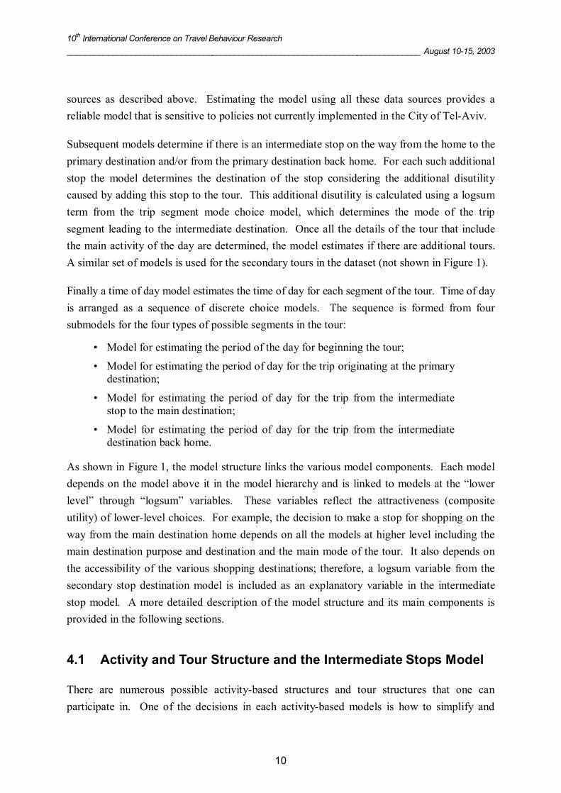
Subsequent models determine if there is an intermediate stop on the way from the home to the primary destination and/or from the primary destination back home. For each such additional stop the model determines the destination of the stop considering the additional disutility caused by adding this stop to the tour. This additional disutility is calculated using a logsum term from the trip segment mode choice model, which determines the mode of the trip segment leading to the intermediate destination. Once all the details of the tour that include the main activity of the day are determined, the model estimates if there are additional tours. A similar set of models is used for the secondary tours in the dataset (not shown in Figure 1).

Finally a time of day model estimates the time of day for each segment of the tour. Time of day is arranged as a sequence of discrete choice models. The sequence is formed from four submodels for the four types of possible segments in the tour:

• Model for estimating the period of the day for beginning the tour;

• Model for estimating the period of day for the trip originating at the primary destination;

• Model for estimating the period of day for the trip from the intermediate stop to the main destination;

• Model for estimating the period of day for the trip from the intermediate destination back home.

As shown in Figure 1, the model structure links the various model components. Each model depends on the model above it in the model hierarchy and is linked to models at the “lower level” through “logsum” variables. These variables reflect the attractiveness (composite utility) of lower-level choices. For example, the decision to make a stop for shopping on the way from the main destination home depends on all the models at higher level including the main destination purpose and destination and the main mode of the tour. It also depends on the accessibility of the various shopping destinations; therefore, a logsum variable from the secondary stop destination model is included as an explanatory variable in the intermediate stop model. A more detailed description of the model structure and its main components is provided in the following sections.

4.1 Activity and Tour Structure and the Intermediate Stops Model

There are numerous possible activity-based structures and tour structures that one can participate in. One of the decisions in each activity-based models is how to simplify and


11

aggregate these various structures to a reasonable number of alternatives to include in the model. In this model it was decided to include up to one intermediate stop on the leg from home to the main destination and up to one intermediate stop on the leg from the main destination to home. Therefore there are only four possible tour structures:

• Home-Main-Home • Home-Intermediate-Main-Home

• Home-Main-Intermediate-Home • Home-Intermediate-Main-Intermediate-Home

The model structures considers the choice of the main destination and the main mode of the tour as higher hierarchy choices, and the choice of the tour structure is following these models and done by estimating a model of whether one make a stop on the way to the primary destination, on the way back and for what purpose. The choices from these models determine the tour structure and the stop various purposes. Avoiding the need to model more than one intermediate stops in each leg significantly simplified the model without loosing a lot of information as these four alternatives include about 95 percent of all the tours. Table 1 shows the distribution of these tour types for primary tours and secondary tours.

The structure of the daily activity pattern is determined by the main tour and by similar set of models to determine if there is a secondary tour and the details of this secondary tour similar to the details of the main tour. Table 2 shows that roughly 40 percent of the activity patterns

Table 1 Tour-Type Distribution

Tour Type Frequency Percentage

Main

Home-Main-Home 22,373 79.0 Home-Intermediate-Main-Home 2,188 7.7

Home-Main-Intermediate-Home 3,015 10.6 Home-Intermediate-Main-Intermediate-Home 759 2.7

Secondary Home-Main-Home 5,766 83.7 Home-Intermediate-Main-Home 519 7.5

Home-Main-Intermediate-Home 471 6.8 Home-Intermediate-Main-Intermediate-Home 131 2.0


12

in the NTHS dataset include no tours. Almost half of the records consist of a singly tour and another 11 percent have a total of two tours per day. Since only two percent of the records have three or more tours, and to simplify the model structure it was decided to model only up to two tours per day.

Table 2 Number of Tours Per Day in the NTHS Dataset

No Tour 1 Tour 2 Tours 3 Tours 4 Tours 5+ Tours

18,637

(39.9%)

22,192

(47.5%)

4,939

(10.6%)

723

(1.6%)

141

(0.3%)

55

(0.11%)

4.2 Mode Choice Modeling

In defining the main modes of the tour and the submodes for the trip segments of the tour three main issues were considered. First the modes should be responsive to policy issues likely to be tested, Second, they should be supported by the data, third, they should be as consistent as possible with the previous NTA model to best make use of both data sources.

There are two main approaches for mode choice analysis in activity-based models, the first approach defines each combination of modes in the tour as an alternative and the second use a two-tier type models, where, first the main mode choice of the tour is determined as one of few main modes, and a second tier where the exact mode of each segment of the tour is determined given the main mode of the tour. Data analysis in support of the decision regarding the mode choice model structure showed that about 91 percent of all tours are single mode tours. Out of the other nine percent tours little more than half are combinations of bus and auto passengers and the rest are small frequencies of a lot of different combinations.

Therefore, more emphasis was devoted to the tour main mode, and secondary efforts to model segments’ modes as deviations from the tour main mode. The tour main mode was defined as the mode of the segment leaving home. Given that more than 90 percent of the tours have a single mode for all segments the definition is of secondary importance, as alternative definitions will not change the tour main mode for most of the tours. However, defining the tour main mode as the mode leaving home makes sense as this constrains the modes of the following segments. For example, if you left without a car you are not likely to use car for following segments. The segment mode choice model will model deviation from the main mode in each of the tour segments following the first segment.


13

The tour main mode model is being estimated using all available data sources including the NTA SP data, the new SP data, the NTHS RP data and the Rail Corridor RP data. First a joint SP model on the two SP data sources was estimated. In the next phase a joint RP model on the two RP data sources will be estimated, and finally a combined RP-SP model will be estimated. The tour main modes are defines as follow:

• Auto driver

• Auto passenger • Premium transit

- Walk access - Bus access

- Kiss-and-Ride (K&R) access - Park-and-Ride (P&R) access

• Bus only - Walk access

- Kiss-and-Ride (K&R) access - Park-and-Ride (P&R) access

• Taxi • (Employer Provided Transportation)

Employer Provided Transportation (EPT) is not part of the mode choice model but will be determined externally to the model. EPT is nine percent of all tours as tour main mode and while not included in the mode choice they are included for all other model components. The taxi mode has a share of only 1.3 percent in the NTHS, but 18 percent of the travelers in the SP chooses taxi. While part of this may be bias, it also may show that it may be an important mode for policy response and it is therefore an important mode.

The same modes are used for the tour segments mode choice model. In most cases the mode of the segment will be the same as the tour mode, however it may be any other mode with some availability constraints. Both multinomial and nested models were tested. In the nested version the first level is a decision between: Same – meaning the mode of the segment is the same as the main mode; and Switch – meaning the person is switching to another mode. Under the switch there is a nest with the possible alternative modes.


14

5. Selected Model Estimation Results

As this is a work in progress only few models have been estimated to date and the results are intermediate ones, as all model estimation will be revised once all the data sources will be used. In nested models we start the model estimation from the lower levels to the higher ones, so we can calculate logsum variables from lower-level models to be includes as accessibility variables in higher-level models. The lowest-level model is the segment mode choice for the secondary tour. However, only 384 out of the 15,032 trip segments in secondary tours had different modes than the main mode. In other words in 97.4 percent of the cases there was no mode switching in secondary tours. Therefore, it was decided to have this as a deterministic model, assuming all trips of secondary tours have the same mode choice as the main mode chosen for the tour.

5.1 Secondary Tour Intermediate Stop Destination Choice

Given that there is no mode choice model for trips of the secondary tours this is the lowest model estimated in the model hierarchy. This model estimates the probability that a person making an intermediate stop in a secondary tour will choose each zone as his destination. The model includes stops made before and after the main activity in the secondary tour. Both the Tel-Aviv household survey data and the rail corridor survey data have been used in the estimation of this model.

In calculating the level of service variables the concept of “additional travel time” is used. This variable represents the additional travel time due to the destination being added to the tour as previously defined. For example, in the case of an intermediate stop before the main destination, this travel time equals the time from home to the intermediate stop plus the time from the intermediate stop to the main destination minus the time from home to the main destination. In other words, this is the additional travel time the person has to make from his home to the main destination because he decided to make a stop in between.

The mode of travel for the trips in the secondary tour are all determined by the tour mode choice model which is of higher hierarchy, and therefore, there is no need to calculate log sum from lower-level mode choice models and the LOS variables of the chosen mode are used. Similar to the additional travel time, there are other additional LOS variables, such as additional transfers, additional parking cost, and additional wait time.

There are a total of 1,248 observations for intermediate stop destinations, most of them for the “other” purpose and only about 100 observations for each of the work (including commute,


15

work-related and education) and shop purposes, therefore one model was estimated for all purposes. There are 1,219 destination choice zone alternatives for each individual and all 1,219 were modeled as alternative choices. Only 448 zones (37 percent) out of these 1,219 zones were actually chosen as intermediate stop destinations.

Table 3 shows the model estimation results for this model.

Table 3 Intermediate Stop Destination Choice Model

Variable Coeff. t-Statistic Description

Auto Travel Time -0.1119 -41.4 Additional auto travel time in minutes

Parking Walk Time -0.0103 -0.4 Time to walk from parking to destination in minutes

Parking Search Time -0.1053 -2.0 Time to search for parking in minutes

Transit Travel Time -0.0531 -5.5 Additional transit travel time in minutes

Number of Transfers -0.2039 -0.8 Additional number of transfers for transit passengers

Area Type Indicators

Cultural area indicator

Educational area indicator

Office area indicator

Shop area indicator

Other area type indicator

0.1751

0.2124

0.3882

-0.0265

0.1900

2.9

3.0

5.4

-0.4

2.8

These are not mutually exclusive

0/1 indicator if zone has cultural centers

0/1 indicator if zone has educational centers

0/1 indicator if zone has office centers

0/1 indicator if zone has shopping centers

0/1 indicator if zone has other type centers

Zone Classification

Open space

CBD zone dummy

Fringe CBD zone dummy

Industrial zone dummy

Residential zone dummy

0

0.2975

-0.3481

-0.8474

-0.2907

1.8

-2.5

-4.7

-3.3

These are mutually exclusive

Takes value 1 if zone is classified as CBD, else 0

Takes value 1 if zone is classified as just outside CBD, else 0

Takes value 1 if zone is classified as industrial, else 0

Takes value 1 if zone is classified as residential, else 0

Total Employment 0 0 Total employment in the zone

Population -0.2155 -1.2 Total population in the zone

Summary Statistics

Log likelihood at zero Log Likelihood at Constants Final Log Likelihood “Rho-Squared” w.r.t. Zero “Rho-Squared” w.r.t. Constants

-8868.02 -7293.26 -6286.17

0.291 0.137


16

All the level of service variables have the expected negative signs with auto travel time, parking time, and transit time being significant, and parking walk and number of transfers not significant. These measures of impedance reflect the greater attractiveness of closer-by (as measure by the “additional” concept) destination zones for intermediate stops during the secondary tour. Travel time sensitivity is greater among auto drivers than transit riders. In model estimation we also tried to test the effect of the parking cost variable but it resulted with a counterintuitive positive coefficient. This variable is highly correlated with the area type dummies and may simply indicates that people prefer going to the CBD to fulfill their needs despite the cost incurred due to parking. The location dummies clearly indicate the attractiveness of intermediate stops located in the CBD compared to any other type of destination (least attractive being the industrial zones). It is important to note from the data that open spaces are not truly empty spaces. Zones indicated as open spaces in the data have various types of employment and population residing in them. The “qualitative” zone indicator variables highlight the greater attractiveness of zones with offices, cultural attractors, and zones with “other” attractors. Finally, total employment and population are the size variables showing the higher probability of larger zones to be selected as destination zones. The employment is used as the reference variable with smaller contributions by population. One should remember that these coefficients are in exponent forms and the actual size coefficients are therefore positive.

5.2 The SP Main Mode Choice

As discussed above the main mode (or the tour mode) choice SP model is a combined model using both the stated-preference collected for this master plan study (SPMP) and the NTA Stated-preference (NTASP) data previously available.

Separate models were estimated for each travel purpose. We present here the structure and results for the work trips purpose. For the SPMP survey, a distinction could be made between primary and secondary tours: two-thirds of the observations belong to primary tours, one-third to secondary tours. The NTASP data cannot give information on this. This means that we could try to have some coefficients in the SPMP split between primary and secondary tours. However if we would do this, it is no longer possible to have common coefficients in SPMP and NTASP. We tried separate primary and secondary tour models on the SPMP data alone and only for ‘other’ purposes were we able to get acceptable split estimation results. In the combined NTASP and SPMP model we did not use this distinction because we want to have common coefficients on both databases.


17

In the SPMP model 10 alternatives were defined:

• Alternative 1 bus with walk access

• Alternative 2 bus with kiss-and-ride (K&R) access • Alternative 3 bus with park-and-ride (P&R) access

• Alternative 4 mass transit (MT) with walk access • Alternative 5 MT with K&R access

• Alternative 6 MT with P&R access • Alternative 7 MT with bus access

• Alternative 8 car driver • Alternative 9 car passenger

• Alternative 10 taxi

In the NTASP model nine alternatives were defined (as in the report ‘NTA model improvement study: development of the mode choice model’ by Hague Consulting Group, 2000):

• Alternative 11 bus with walk access

• Alternative 12 bus with K&R access • Alternative 13 bus with P&R access

• Alternative 14 MT with walk access • Alternative 15 MT with K&R access

• Alternative 16 MT with P&R access • Alternative 17 MT with bus access

• Alternative 18 car driver • Alternative 19 car passenger

In the estimation of the combined SPMP – NTASP model system, the utility functions of the SPMP and NTASP models share as much coefficients as possible. This implies that the tradeoffs (or marginal rates of substitution) among some of the attributes are the same in the SPMP and NTASP data. Other coefficients are specific to either the MP or to the NTA utility functions. The level of randomness in the data sources may vary and their relative difference is captured by the NTA scale parameter.

The structure of the model is displayed in Figure 2. The tree for the combined estimation has two subtrees. The NTASP subtree on the right side of the figures is augmented with nine dummy nodes at the bottom. These dummy nodes are there to include a different scale for the NTASP model.


18

Figure 2 Combined SPMP – NTASP Model Structure for Work Trips

1Bus

Walk

2Bus

K&R

3BusP&R

4MT

Walk

5MT

K&R

6MT

P&R

7MTBus

8Car

Driv.

9Car

Pass.

10Taxi

Level 2Public

TransportPrivateMeans

Level 1Bus MT

NTA Scale

11Bus

Walk

12Bus

K&R

13BusP&R

14MT

Walk

15MT

K&R

16MTP&R

17MTBus

18Car

Driv.

19Car

Pass.

SPMP Alternatives

NTASP Alternatives

Table 4 presents the coefficient names and definitions used in the SPMP and NTASP utility equations and the estimation results. As can be seen from the table all of the level of service variable have the right sign and are significant except the bus and mass transit number of transfers. This model is unique in the number and variety of the level of service variables available for policy analysis including in addition to the traditional cost, in vehicle travel time, wait and walk time for the various modes, car parking search time, car parking walk time, and car parking cost both for the car mode and for the car as an access mode to public transportation.


19

Table 4 The Work Purpose SP Model Estimation Results

Coef. Name Coef.

Estimate t-statistic

Definition

bkco -3.28 -18.4 Bus with K&R access constant mtwco 0.499 3.6 MT with walk access constant mtkco -1.31 -7.3 MT with K&R access constant Mtpco 0.810 1.5 MT with P&R access constant Cardco -1.45 -4.0 Car driver constant Carpco -2.23 -7.5 Car passenger constant Taxico -0.845 -3.9 Taxi constant Binvt_c -0.0419 -14.0 Bus in vehicle travel time Bovt_c -0.0487 -8.1 Bus wait time and transfer time Minvt_c -0.0357 -13.9 MT in vehicle travel time Movt_c -0.0507 -7.6 MT wait time and transfer time Cinvtd_c -0.0456 -10.7 Car driver in vehicle travel time Cinvtp_c -0.0263 -4.8 Car passenger in vehicle travel time Ttime_c -0.0191 -3.4 Taxi in vehicle travel time Cfueld_c -4.5e-4 -3.9 Car driver fuel cost Cfuelp_c -0.0014 -6.0 Car passenger fuel cost Ctolld_c -2.9e-4 -2.7 Car driver toll costs Ctollp_c -5.0e-4 -2.0 Car passenger toll costs Tcost_c -0.0015 -13.0 Taxi cost Ptcost_c -0.0014 -13.8 Public transport fare Bxfer_c 0.0929 1.6 Bus number of transfers Mxfer_c -0.0445 -0.8 MT number of transfers Cpcost_c -2.5e-4 -3.1 Car parking cost Cpst_c -0.0476 -3.9 Car parking search time Cpwt_c -0.0442 -3.6 Car parking walk time LRT_c -0.461 -4.1 MT Light Rail train mode SR_c -0.616 -5.4 MT Suburban Rail mode EB_c -0.842 -6.6 MT Enhanced Bus mode LRT_SR_c -0.348 -3.0 MT Light Rail/Suburban Rail mode LRT_M_c -0.448 -4.1 MT Light Rail/Metromode LRT_EB_c -0.486 -4.5 MT Light Rail/Enhanced Bus mode SR_EB_c -0.604 -5.4 MT Suburban Rail/Enhanced Bus mode SR_M_c -0.301 -2.9 MT Suburban Rail/Metro mode M_EB_c -0.606 -5.5 MT metro/Enhanced Bus mode Busage60+ 1.36 4.0 Dummy for bus passenger of 60 years and older Cpsage1625 0.613 2.6 Dummy for car passenger in the age of 16 to 25 Cdredu14 0.366 3.1 Dummy for car driver who studied more than 14 years Taxedu14 0.569 3.7 Dummy for car passenger who studied more than 14 years cpsoccuwpt -1.70 -3.9 Dummy for car passenger who work part-time Ptawt_c -0.0826 -12.8 Public transport access walk time Ptadt_c -0.0427 -8.2 Public transport access drive time Ptapc_c -0.0014 -6.4 Public transport access parking cost Ptapws_c -0.0390 -2.5 Public transport access parking walk and search time Ptakca1 0.171 4.3 Public transport with K&R access one car availability Ptapca1 -3.77 -7.6 Public transport with P&R access one car availability


20

Ptakca2 0.330 6.3 Public transport with K&R access two car availability Table 4 The Work Purpose SP Model Estimation Results (continued)

Coef. Name Coef. Estimate

t-statistic

Definition

Ptapca2 -3.56 -7.1 Public transport with P&R access two car availability Cdca1 0.935 3.4 Car driver one car availability Cdca2 1.49 5.4 Car driver two or more cars availability Cpca1 -0.379 -2.3 Car passenger one car availability Cpca2 0.0516 0.3 Car passenger two or more car availability Bakr -1.03 -11.4 Bus with K&R access constant Bapr 2.98 5.9 Bus with P&R access constant Mawalk 0.763 7.1 MT with walk access constant Makr -0.386 -3.1 MT with K&R constant Mapr 3.85 7.5 MT with P&R constant Mabus 0.164 1.4 MT with bus access constant Cardr -1.50 -4.5 Car driver constant Carpass -0.987 -4.1 Car passenger constant delay -0.0206 -3.3 Public transport probability of delay more than 10 minutes Seat 0.0284 3.5 Public transport probability of finding a seat Logsum1 0.618 12.1 NTA scale coefficient Logsum2 0.655 10.0 NTA scale coefficient Scale 2.58 11.2 NTA scale factor to combine with MP Final log likelihood -7090.5 No. observations 5612 Rho-sq. (0) 0.307 Rho-sq. (C) 0.142

The resulting values of time from this model are 18 NIS ($ 1 = 4.5 NIS) for bus, 15.3 NIS for mass transit, 60.8 NIS for car driver, 11.3 NIS for car passenger and 7.6 NIS for taxi. These values are reasonable, expect the taxi value of time that is somewhat low.

6. Application

The application of the model for forecasting uses a ‘sample enumeration’ approach with a representative sample of households. A Monte Carlo simulation is used to estimate the decisions of the prototype sample and expand it to the entire population. The model simulates for each individual the decisions regarding his main activity for the day, the location of this activity, and all the related travel decisions, including the mode used to travel there, the number and type of stops made on the way there or back, and the timing of all these different activities and trips. Once the model creates tours for the whole population, these tours are


21

broken down to trip segments to create a daily person origin-destination trip tables by mode for purposes of network assignment.

6.1 Population Generation and Forecasting

The first step in the application procedure is to generate the base year synthetic population and to forecast it for the future year. In creating the base year synthetic population the following data will be used:

• The 1996/1997 Census data

• The NTHS sample • Forecast of marginal demographic data (similar to the type of information

appear in the census data)

The objective is to create a synthetic population over TAZs that maintain the statistical characteristics of the Census. However, the Census data do not provide cross-classified demographics. Because the NTHS contains complete household records we can obtain cross-classified estimates from this sample. The general idea is to use iterative proportional fitting (IPF) of the census summaries to the cross-classified values obtained from the NTHS. In other words, the NTHS represents a sample/seed and the Census data gives the marginal totals. IPF estimates the entries in the sample multi way table to make them exactly match the known margins while maintaining the sample table’s correlation structure. The same procedure can be used to update the synthetic population for future years. Future forecasts of variables will be used as the new margins instead of those based on the Census for the base year.

7. Conclusions

This paper presented the development of a new activity-based model for Tel-Aviv. Continuous increases in traffic congestion and other transport negative externalities has led to increasing need for policy-makers to implement travel demand management policies. Traditional modeling tools, however, are not sufficient to understand travelers’ response to such policies. While this paper presents work in progress, initial results show that it will provide a powerful and a practical tool to better understand travel behaviour helping policy-makers to better analyze the benefits and costs from implementing different transportation policies. The model benefits from a wide variety of data including a tour-based stated-preference survey and a detailed parking survey, enabling the model to include important new policy variables such as congestion pricing, parking search time and walking time from the


22

parking to the destination. This model estimates travelers’ response to policies affecting such variables based on people responses to these specific variables and in a comprehensive framework that can analyze their effect on the person’s daily activity schedule therefore making the estimated response more realistic. Further research and applications are needed to better develop and implement this approach for a wide variety of policy analysis.

8. References

Algers, S., A. Daly, P. Kjellman and S. Widlert, (1995) Stockholm Model System (SIMS): Application, 7th World Conference of Transportation Research, Sydney, Australia, 1995.

Algers, S. and M. Beser (2000), ‘SAMPERS – The new Swedish national travel demand forecasting tool’, Paper presented at the IATBR 2000 conference, Gold Coast, Australia.

Arentze, T., Hofman, F. and Timmermans, H. Predicting multifaceted activity-travel adjustment strategies in response to possible congestion pricing scenarios using an Internet-based stated adaptation experiment. Transport Policy, In Press, Corrected Proof.

Axhausen K.W. and Garling T. (1992) Activity-Based Approaches to Travel Analysis: Conceptual Frameworks, Models and Research Problems. Transport Reviews 12(4): pp. 323-341.

Ben-Akiva M. and Bowman J.L., (1998) Activity-Based Travel Demand Model Systems. In: Equilibrium and Advanced Transportation Modeling, Kluwer Academic Publishers, Boston, MA. Pp. 27-46.

Bonnel, P. (1995) An Application of Activity-Based Travel Analysis to Simulation of Change in Behavior. Transportation 1995/02 22(1) pp. 73-93.

Bowman, J.L., M. Bradley, Y. Shiftan, T.K. Lawton and M. Ben-Akiva. (1998) Demonstration of Activity-Based Model System for Portland in World Transport Research, Selected Proceedings from the 8th World Conference on Transport Research, Antwerp, Belgium, July, edited by H. Meersman, E. Van de Voorde, and W. Winkelmans, Elsevier Science Ltd.

Bowman, J. L. and Ben-Akiva, M. E. (2001) Activity-based disaggregate travel demand model system with activity schedules. Transportation Research Part A: Policy and Practice, 35, 1-28.

Bhat C.R., and F. Koppelman (1999) A Retrospective and Prospective Survey of Time-Use Research. Transportation 26(2) pp. 119-139.

Cambridge Systematics, Inc. (1996a) Data Collection in the Portland, Oregon Metropolitan Area, prepared for the Travel Model Improvement Program, Track D – Data Research, U.S. Department of Transportation, Washington, D.C., April.

Cambridge Systematics Inc. (1996b) Appendix B, Description of the STEP Analysis Package in: Quantifying Air Quality and Other Benefits and Costs of Transportation Control


23

Measures Task 3 Analysis Framework Interim Report. Prepared for the National Cooperative Highway Research Program, Project 8-33.

Cambridge Systematics, Inc., (1997) A System of Activity-Based Models for Portland, Oregon, Draft Report of a Demonstration Project for the FHWA Transportation Model Improvement Program, November.

Cascetta, E., and L. Biggiero, (1997), Integrated Models for Simulating the Italian Passenger Transport System in Papageorgiou M. and A. Poulezos (Ed.) Transportation Systems, Preprints of the 8th IFAC/IFIP/IFORS Symposium, Chania, Greece.

Ettema, D. and Timmermans H. (1997) Theories and Models of Activity Patterns. In: Ettema, D. and Timmermans H. (eds.) Activity-Based Approaches to Travel Analysis (pp. 1-36) Oxford: Pergamon.

Garling, T., M.P. Kwan and R.G. Golledge (1994) Computational-Process Modeling of Household Activity Scheduling. Transportation Research B, 28B(5), pp. 355-364.

Gunn, H.F., A.I.J.M. and Van der Hoorn, A. (1998) The Predictive Power of Operational Demand Models. Paper D14, prepared for the European Transport conference, Loughborough University, September. London: Proceedings of the Seminar Transportation Planning Methods, ISBN 0-86050-313-5.

HCG and TOI (1990), ‘A model system to predict fuel use and emissions from private travel in Norway from 1985 to 2025’, Report to the Norwegian Ministry of Transport, HCG and TOI.

Jones, p.m. (1983) The Practical Application of Activity-Based Approaches in Transport Planning: An Assessment. In Carpenter S. and P. Jones (Ed.) Recent Advances in Travel Demand Analysis, Gower Publishing, Hanst, England.

Kharoufeh, J. P. and Goulias, K. G. (2002) Nonparametric identification of daily activity durations using kernel density estimators. Transportation Research Part B: Methodological, 36, 59-82.

Kitamura, R. (1997) Applications of Models of Activity Behavior for Activity-Based Demand Forecasting. In Activity-Based Travel Forecasting Conference. Proceedings of the Activity-Based Travel Forecasting Conference in New Orleans, June 1996. U.S DOT, Washington D.C.

Kitamura, R., Pendyala, R.M., Pas, E.I. and Reddy, P. (1995) Application of AMOS, an Activity-Based TCM Evaluation Tool to the Washington, D.C. Metropolitan Area. In 23rd European Transport Forum: Proceedings of Seminar E Transportation Planning Methods. PTRC Education and Research Services, Ltd., London, pp. 177-190.

Kitamura, R., Pas, E. I., Lula, C.V., Lawton, T. K., and Benson, P. E. (1996) The Sequenced Activity Mobility Simulator (SAMS): An Integrated Approach to Modeling Transportation, Land Use and Air Quality. Transportation, 23(3), pp. 267-291.

Mark Bradley Research & Consulting, (1998) A System of Activity-Based Models for Portland, Oregon, Prepared under subcontract to Cambridge Systematics, Inc. as part of the Portland Demonstration Project for the Travel Model Improvement Program, Federal Highway Administration, Washington, D.C., May 1998.


24

Pendyala, R.M., R. Kitamura, C. Chen, and E.I.Pas (1997) An Activity-Based Micro simulation Analysis of Transportation Control Measures. Transport Policy, Vol. 4, No. 3 pp 184-192.

Pickrell D.H. (1990). Urban Rail Transit Projects: Forecasts Versus Actual Ridership and Costs. U.S. Department of Transportation, Report No. DOT-T-01-04.

Recker, W. W. (2001) A bridge between travel demand modeling and activity-based travel analysis. Transportation Research Part B: Methodological, 35, 481-506.

Recker W.W., M.G. NcNally and G.S. Root (1986), A Model of Complex Travel Behavior: Part 2: An Operational Model. Transportation Research, 20A(4), pp. 307-18.

Recker W.W. & A. Parimi. (1999) Development of a Microscopic Activity-Based Framework for Analyzing the Potential Impacts of Transportation Control Measures on Vehicle Emissions. Transportation Research Part D pp. 357-378.

Rossi, T. & Y. Shiftan, (1997) Tour-Based Travel Demand Modeling in the U.S., Proceeding of the 8th IFAC/IFIP/IFORS Symposium on Transportation Systems, Chania, Greece, June.

Ruppert, E. (1998). The Regional Transportation Model “TRANSFER.” Paper presented at the 8th World Conference on Transport Research, Antwerp, Belgium, July 1998.

Scott, D. M. and Kanaroglou, P. S. (2002) An activity-episode generation model that captures interactions between household heads: development and empirical analysis. Transportation Research Part B: Methodological, 36, 875-896.

Shiftan Y. (1999) “A Practical Approach to Model Trip Chaining” Transportation Research Record, No. 1645, pp. 17-23, 1999.

Shiftan Y. and J. Suhrbier. (1998) “The Contribution of Activity-Based Models to Analyses of Transportation Control Measures” in World Transport Research, Selected Proceedings from the 8th World Conference on Transport Research, Antwerp, Belgium, July, edited by H. Meersman, E. Van de Voorde, and W. Winkelmans, Elsevier Science Ltd.

Shiftan Y. & Suhrbier J. (2002) “The Analysis of Travel and Emission Impacts of Travel Demand Management Strategies Using Activity-Based Models” Transportation, Vol. 29, No. 2.

Skamris M. and K. Flyvbgerg-Bent, (1997) Inaccuracy of Traffic Forecasts and Cost Estimates on Large Transport Projects. Transport Policy 7.

Stopher, P.R. (1993). Deficiencies of Travel-Forecasting Methods Relative to Mobile Emissions. ASCE Journal of Transportation Engineering, Vol. 119,5.

Walmsley D.A. and M.W. Pickett (1992). The Cost and Partonage of Rapid Transit Systems Compared with Forecasts. Research Report 352, Transportation Research Laboratory, Department of Transport.

Activity-Based Modeling as a Tool for Better Understanding Travel Behaviour

Documents

Transcript of Activity-Based Modeling as a Tool for Better Understanding Travel Behaviour