University of Rhode Island University of Rhode Island

DigitalCommons@URI DigitalCommons@URI

Open Access Master's Theses

2018

Active Contours Implementation Active Contours Implementation

Steven D. Oberhelman University of Rhode Island, soberhelman@my.uri.edu

Follow this and additional works at: https://digitalcommons.uri.edu/theses

Recommended Citation Recommended Citation Oberhelman, Steven D., "Active Contours Implementation" (2018). Open Access Master's Theses. Paper 1193. https://digitalcommons.uri.edu/theses/1193

This Thesis is brought to you for free and open access by DigitalCommons@URI. It has been accepted for inclusion in Open Access Master's Theses by an authorized administrator of DigitalCommons@URI. For more information, please contact digitalcommons@etal.uri.edu.

ACTIVE CONTOURS IMPLEMENTATION

BY

STEVEN D. OBERHELMAN

A THESIS SUBMITTED IN PARTIAL FULFILLMENT OF THE

REQUIREMENTS FOR THE DEGREE OF

MASTER OF SCIENCE

IN

ELECTRICAL ENGINEERING

UNIVERSITY OF RHODE ISLAND

2018

MASTER OF SCIENCE THESIS

OF

STEVEN D. OBERHELMAN

APPROVED:

Thesis Committee:

Major Professor Frederick J. Vetter

Richard Vaccaro

Manbir Sodhi

Nasser H. Zawia

DEAN OF THE GRADUATE SCHOOL

UNIVERSITY OF RHODE ISLAND

2018

ABSTRACT

Many image processing problems require the detection of objects in an image.

In problems such as these, active contours are widely used to extract features of

interest from an image or model for computer analysis. Many examples of active

contour applications come from biomedical image processing, where both healthy

and diseased areas of the body can be detected, counted, and/or measured; how-

ever, a number of other applications of active contours exist outside of the biomed-

ical field. This paper will survey the state of active contours and deliver software

that can be used to explore the various nuances of active contour application. The

topics in this paper include an explanation of internal energy and external energy

using the Marr method, Gradient Vector Flow (GVF) method, and Vector Field

Convolution (VFC) method. This paper will focus on 2-D active contours, but

almost all of these methods can also be used to fit an active surface to 3-D objects.

In the appendix, a Matlab program is provided that implements these methods.

ACKNOWLEDGMENTS

I would like to sincerely thank my major professor, Dr. Fred Vetter, for all

the support and guidance he has given throughout this work. I am grateful for

the opportunity to work with him on this project. My committee members, Dr.

Richard Vaccaro, and Dr. Monbir Sodhi, also deserve recognition for dedicating

their time to reviewing and providing meaningful feedback for my thesis. I would

also like to thank my defense chair, Dr. Chengzhi Yuan.

I would like to thank my parents for their love and for supporting me in

every way possible and to Vanessa for all of her love, support and proofreading.

Additionally I would like to thank all of my friends and coworkers for their support

throughout the year and to Dr. Koch for his professional guidance and constant

support.

iii

TABLE OF CONTENTS

ABSTRACT . . . . . . . . . . . . . . . . . . . . . . . . . . . . . . . . . . ii

ACKNOWLEDGMENTS . . . . . . . . . . . . . . . . . . . . . . . . . . iii

TABLE OF CONTENTS . . . . . . . . . . . . . . . . . . . . . . . . . . iv

LIST OF FIGURES . . . . . . . . . . . . . . . . . . . . . . . . . . . . . . vi

LIST OF TABLES . . . . . . . . . . . . . . . . . . . . . . . . . . . . . . . viii

CHAPTER

1 Introduction . . . . . . . . . . . . . . . . . . . . . . . . . . . . . . . 1

2 Active Contour Mechanics . . . . . . . . . . . . . . . . . . . . . . 5

2.1 Internal Energy . . . . . . . . . . . . . . . . . . . . . . . . . . . 5

2.2 Edge map . . . . . . . . . . . . . . . . . . . . . . . . . . . . . . 6

2.3 External Energy . . . . . . . . . . . . . . . . . . . . . . . . . . . 8

2.4 Kass, Witkin, and Terzopoulos (KWT) Method . . . . . . . . . 11

3 External Energy . . . . . . . . . . . . . . . . . . . . . . . . . . . . 13

3.1 Gradient Vector Flow (GVF) . . . . . . . . . . . . . . . . . . . . 13

3.2 Vector Field Convolution . . . . . . . . . . . . . . . . . . . . . . 15

4 Active Contours Software . . . . . . . . . . . . . . . . . . . . . . 18

4.1 Active Contours Software Introduction . . . . . . . . . . . . . . 18

4.2 Active Contours Software Performance . . . . . . . . . . . . . . 21

5 Future Work . . . . . . . . . . . . . . . . . . . . . . . . . . . . . . 26

5.1 Splines and Models . . . . . . . . . . . . . . . . . . . . . . . . . 26

iv

Page

v

5.2 Active Surfaces . . . . . . . . . . . . . . . . . . . . . . . . . . . 26

5.3 Active Contour Merging, Ballooning Force and GVF BoundaryConditions . . . . . . . . . . . . . . . . . . . . . . . . . . . . 27

5.4 Generalized Gradient Vector Flow . . . . . . . . . . . . . . . . . 27

5.5 Tracking . . . . . . . . . . . . . . . . . . . . . . . . . . . . . . . 28

5.6 Stopping Criteria . . . . . . . . . . . . . . . . . . . . . . . . . . 28

5.7 Clustering . . . . . . . . . . . . . . . . . . . . . . . . . . . . . . 28

LIST OF REFERENCES . . . . . . . . . . . . . . . . . . . . . . . . . . 29

APPENDIX

A Matlab script . . . . . . . . . . . . . . . . . . . . . . . . . . . . . . 31

B Internal Energy Derivation . . . . . . . . . . . . . . . . . . . . . 38

C Gradient Vector Flow Derivation . . . . . . . . . . . . . . . . . . 39

BIBLIOGRAPHY . . . . . . . . . . . . . . . . . . . . . . . . . . . . . . . 41

LIST OF FIGURES

Figure Page

1 A noisy star image. . . . . . . . . . . . . . . . . . . . . . . . . . 2

2 The edge map of the noisy star image. . . . . . . . . . . . . . . 2

3 The initial active contour on the edge map. . . . . . . . . . . . 3

4 The active contour after a few iterations. The red points arethe most recent iteration of the active contour. The blue linesare past active contours. . . . . . . . . . . . . . . . . . . . . . . 3

5 The final active contour. . . . . . . . . . . . . . . . . . . . . . . 4

6 Using the program developed in this work to determine the edgesof a heart slice . . . . . . . . . . . . . . . . . . . . . . . . . . . 4

7 (Upper Left) Image with row 110 highlighted in red. (UpperRight) Pixel values of image row 110 with grayscale pixel valuesbetween 0 and 1. (Lower Left) Edge map of image row 110 usingEquation 3. (Lower Right) External Energy of image row 110using the KWT method [1]. . . . . . . . . . . . . . . . . . . . . 7

8 The external energy using the Marr method. The black line isthe edge map of the image and the blue vectors indicate thedirection and magnitude of the external force. The left paneluses a Gaussian blur with a standard deviation of 10 while theright panel uses a Gaussian blur with a standard deviation of4. Note how the Marr method that uses Gaussian blur with alarge standard deviation does not create large external energiesnear the edge. . . . . . . . . . . . . . . . . . . . . . . . . . . . 10

9 The external force using the GVF with µ = 0.3. The black lineis the edge map of the image and the blue vectors indicate thedirection and magnitude of the external force. . . . . . . . . . . 15

10 (Left Panel) VFC vector field kernel using the magnitude func-tion from Equation 12, ε = 0.01 and γ = 2. (Right Panel) VFCvector field kernel using the magnitude function from Equation13, ξ = 2. . . . . . . . . . . . . . . . . . . . . . . . . . . . . . . 16

vi

Figure Page

vii

11 The external force using the VFC with ξ = 6 in Equation 13.The black line is the edge map of the image and the blue vectorsindicate the direction and magnitude of the external force. . . . 17

12 Demonstration of Active Contour Program. . . . . . . . . . . . 18

13 Image to test the program developed in this work. . . . . . . . . 21

14 Marr external energy test using the test image in Figure 13 . . . 23

15 VFC external energy test using the test image in Figure 13 . . . 24

16 GVF external energy test with an initial external energy usingthe Marr approach using the test image in Figure 13. . . . . . . 25

LIST OF TABLES

Table Page

1 List of variables . . . . . . . . . . . . . . . . . . . . . . . . . . . 20

viii

CHAPTER 1

Introduction

An active contour is a thin curve on an image that can delineate a desired

feature. Active contours are used in image processing to extract features of interest

from an image or model for computer analysis. An active contour is defined as a

list of ordered points or as a continuous parametric function (x(s), y(s)) where the

range of s is defined; typically, sε[0, 1]. The active contour forms to the edge of

an object by minimizing a summation of energies which gives the active contour

its properties. The two main energies are internal and external energy, but others

like a ballooning force [2] can be included [3] [1].

To demonstrate an active contour, consider the image in Figure 1. We then

generate the edge map which is explained in section 2.2. The edge map is large

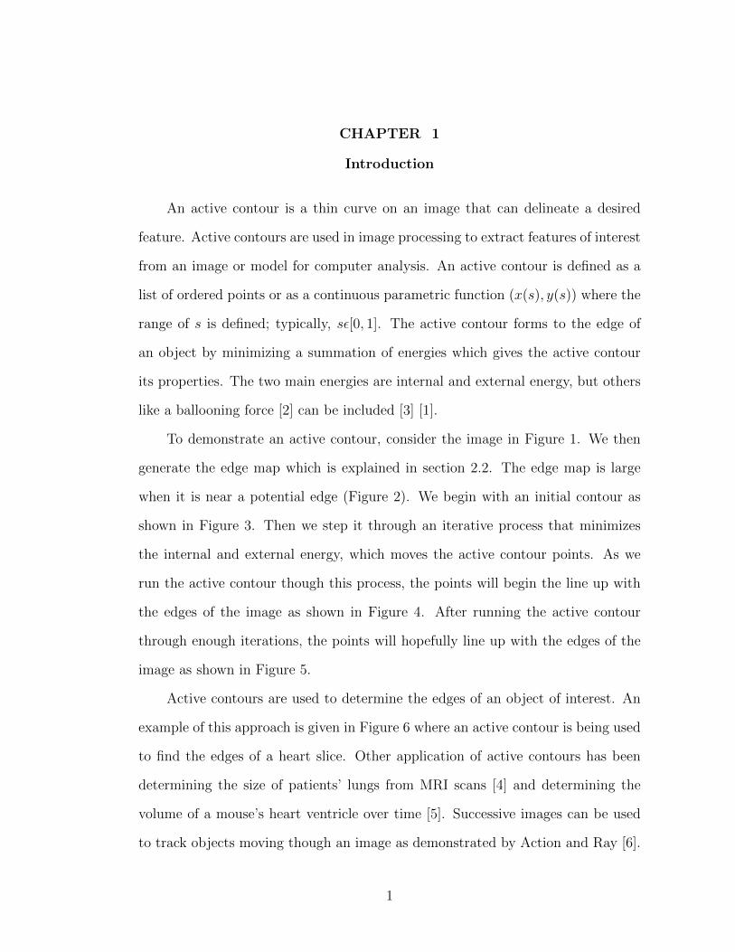
when it is near a potential edge (Figure 2). We begin with an initial contour as

shown in Figure 3. Then we step it through an iterative process that minimizes

the internal and external energy, which moves the active contour points. As we

run the active contour though this process, the points will begin the line up with

the edges of the image as shown in Figure 4. After running the active contour

through enough iterations, the points will hopefully line up with the edges of the

image as shown in Figure 5.

Active contours are used to determine the edges of an object of interest. An

example of this approach is given in Figure 6 where an active contour is being used

to find the edges of a heart slice. Other application of active contours has been

determining the size of patients’ lungs from MRI scans [4] and determining the

volume of a mouse’s heart ventricle over time [5]. Successive images can be used

to track objects moving though an image as demonstrated by Action and Ray [6].

1

Figure 1. A noisy star image.

Figure 2. The edge map of the noisy star image.

2

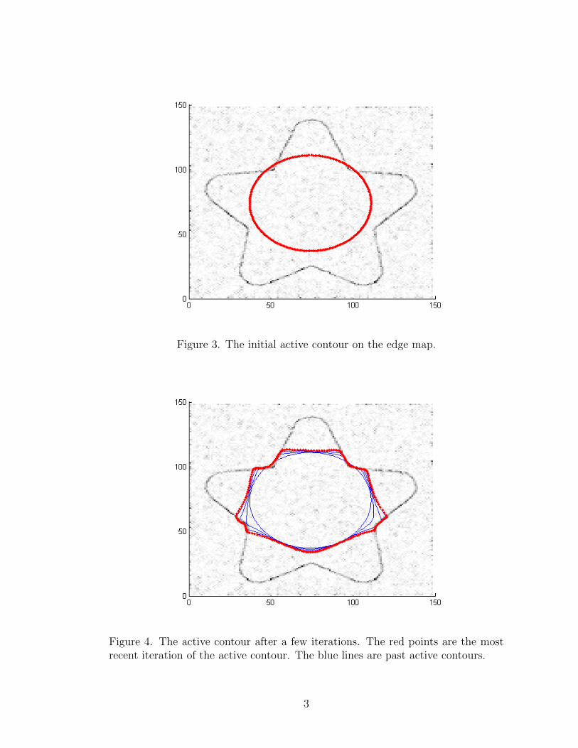
Figure 3. The initial active contour on the edge map.

Figure 4. The active contour after a few iterations. The red points are the mostrecent iteration of the active contour. The blue lines are past active contours.

3

Figure 5. The final active contour.

Figure 6. Using the program developed in this work to determine the edges of aheart slice

4

CHAPTER 2

Active Contour Mechanics

2.1 Internal Energy

The internal energy is defined in such a way that it is minimized when the

active contour is smooth. This will prevent the resulting contour from being jagged,

which makes sense since most edges of interest are smooth. There are two common

ways of representing an active contour and each way has a different way of defining

the internal energy. The first way is an active contour can use a list of points to

define the active contour and the internal energy is minimizing an approximation

of the first and second derivative of the contour. This is the method used in this

paper. The second method is by using splines or parametric equations to represent

the active contour [7] [1]. The internal energy of the active contour is then created

from the constraints placed on it by the spline.

Since we are using a list of points for the active contour, we will define by two

scaling factors which weigh the first and second derivatives of the active contour

to create the internal energy. Conventionally, these weighting factors are α for the

first derivative and β for the second derivative. The Terzopoulos (KWT) active

contour model defines the internal energy as [1]:

Eint(X, Y ) =1

2

∫ 1

0

α

[∣∣∣∣∣dXds∣∣∣∣∣2

+

∣∣∣∣∣dYds∣∣∣∣∣2]

+ β

[∣∣∣∣∣d2Xds2∣∣∣∣∣2

+

∣∣∣∣∣d2Yds2∣∣∣∣∣2]ds (1)

This definition of the active contours results in an internal energy that is minimized

when the first and second derivative are minimized, which occurs when the active

contour is smooth.

With the internal energy defined, we can calculate the internal energy force.

This force needs to “push” the active contour to reach a state with minimal internal

energy. This is done by taking the derivative of the internal energy with respect

5

to the equation of the active contour. Just like the derivative of a function, the

derivative in respect to an equation produces a gradient which can be used to find

a direction to a local minima. Taking the derivative of this internal energy in

Equation 1 results in the following internal forces (Derivation in Appendix B):

Fint X(X) = α∂2X

∂s2− β∂

4X

∂s4(2a)

Fint Y(Y ) = α∂2Y

∂s2− β∂

4Y

∂s4(2b)

2.2 Edge map

Before looking at the external energy of an image, it is worth looking at

the edge map, Iedge(x, y). The edge map is a two dimensional set of values that

measure the change in the gradient in the image. The assumption being made here

is that there is a quick change in color between the object and the background that

occurs at the edge of the object. Many papers define the negative edge map as [1]:

Iedge(x, y) = |∇I(x, y)|2 (3)

A demonstration of the edge map is given in Figure 7. Instead of focusing on

the whole image, the figure will demonstrate the edge map on a one dimensional

case. The upper right panel of Figure 7 shows the pixel grayscale value between 0

(white) and 1 (black) from pixel row 110 of the upper left panel. The edge map of

this row is shown in the lower left panel of Figure 7. As we can see, the peaks of

the edge map at pixel index 50 and 79 correspond with the large change in pixel

values which correspond with the edges of the image.

There are other methods that exist to find an edge map of the image. One

of these approaches is the Canny filter which optimizes the edge map detection

based on assumptions on the size of the object of interest and the amount of noise

present in the image [8].

6

Figure 7. (Upper Left) Image with row 110 highlighted in red. (Upper Right) Pixelvalues of image row 110 with grayscale pixel values between 0 and 1. (Lower Left)Edge map of image row 110 using Equation 3. (Lower Right) External Energy ofimage row 110 using the KWT method [1].

7

2.3 External Energy

The external force “pushes” the active contour points to the edge of the object

of interest. There are many different ways of defining this external energy. This

section is going to look at one of the earliest methods of determining the external

energy, the Marr method [9].

The Marr method was developed by D. Marr [9]. The Marr method uses a

definition of the external energy and then finds the derivative of this function to

find the external force. The external energy in this case is defined in such a way

that it is minimized when the active contour sits near the edge of the feature of

interest:

Eext(x, y) = −∣∣∣∇[G(x, y) ∗ I(x, y)

]∣∣∣2 (4)

where I(X, Y ) is the image, G(x, y) is a Gaussian blur, ∗ is the 2-D convolution

operation, ∇ is the vector gradient operation, and |·| is the magnitude of the vector.

To understand this approach, we first notice that if we remove the Gaussian blur,

then this equation would be the same as the negative edge map (Equation 3).

There are two effects that the Gaussian blur convolution has on this equation.

First, the Gaussian blur spreads out the sharp changes in gradient so that active

contour points that are further away from the edge will be “pulled” towards that

edge (note the difference in width around pixels 50 and 79 between the two spikes

in the bottom panels of Figure 7) [10]. Second, if the image is slightly blurry, the

edge can span over multiple pixels with a weaker gradient. The Gaussian blur will

combine these gradients in such a way that their total energy will be near the same

as a sharp edge that has a large gradient between a few pixels.

An easy way to visualize this phenomenon is to picture the one dimensional

version of this external energy as shown in Figure 7. The bottom right panel in

Figure 7 shows the results of using the Marr method on row 110 of pixels shown

8

in the upper right panel. The Gaussian blur used in the bottom right panel has a

standard deviation of 5. As mentioned before, the edge is located at pixel indexes

50 and 79. These are the points where the Marr method is minimized but with

the added benefit of the wide slow monotonic slope on either side. We can use

this definition of the external energy to find an equation for the external force by

taking the negative gradient of the external energy. This will “push” the active

contour points towards the minima, which hopefully is an edge in the image. The

resulting equation for the external force is:

Fext(x, y) = ∇∣∣∣∇[G(x, y) ∗ I(x, y)

]∣∣∣2 (5)

Since the external force is a vector, it can be broken up into x and y compo-

nents. In this paper, Fext X(x, y) is the x component of the external force vector

and Fext Y(x, y) is the y component of the external force vector.

One thing to note about this approach is that the range is limited in the

Marr method. For example if the active contour point in the lower right panel of

Figure 7 began at pixel index 130, the gradient of the external energy would be

near zero. This would mean that there would be almost no external force on that

active contour point. One way to fix this is to use a wider Gaussian blur which

would cause the points from further away to be drawn in, but then the forces near

the edge will be weakened [10]. This can be seen in the 2-D visualization of the

Marr method shown in Figure 8. Note how the vectors in the left panel are really

small in the immediate vicinity of the edge while the vectors in the right panel are

large in the immediate vicinity of the edge. One way to overcome this issue is to

use multiple external energy maps when updating the active contour. The first

external energy maps will use a wide Gaussian blur (high σ) to “pull” the active

contour points nearby and final external energy maps will use a narrow Gaussian

blur (low σ) to “pull” the active contour points to the edge [10]. This change in

9

Figure 8. The external energy using the Marr method. The black line is the edgemap of the image and the blue vectors indicate the direction and magnitude of theexternal force. The left panel uses a Gaussian blur with a standard deviation of10 while the right panel uses a Gaussian blur with a standard deviation of 4. Notehow the Marr method that uses Gaussian blur with a large standard deviationdoes not create large external energies near the edge.

the external energy will increase the effective range and accuracy of the external

force, but it is still limited in how far the force for an edge can reach before being

lost in the noise. There are other ways of defining the external energy force, and

more of these approaches will be discussed in the next chapter.

Another thing to note about this approach is that the external energy is

typically pre-calculated at the pixel locations of the image but the active contour

points can fall anywhere on the image, even between pixels. This means that when

the active contour is being updated, the external forces on the active contour points

will have to be interpolated. For this paper and for the program developed in this

work, the bi-linear interpolation is used.

10

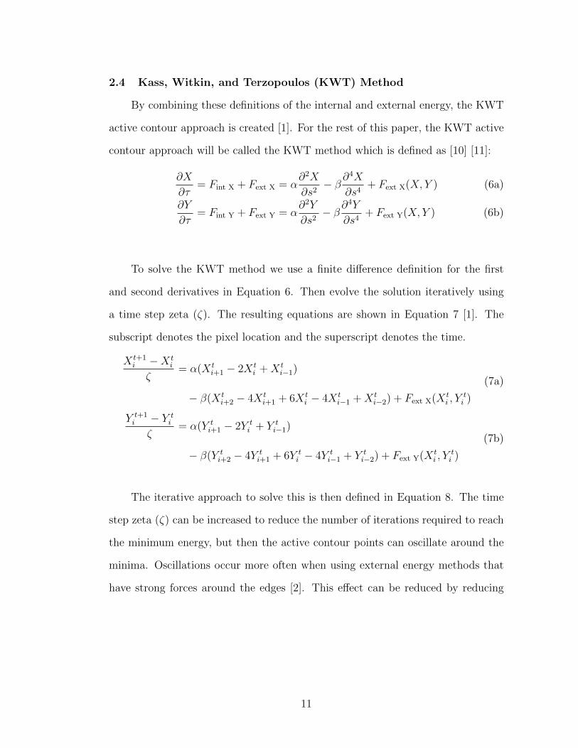
2.4 Kass, Witkin, and Terzopoulos (KWT) Method

By combining these definitions of the internal and external energy, the KWT

active contour approach is created [1]. For the rest of this paper, the KWT active

contour approach will be called the KWT method which is defined as [10] [11]:

∂X

∂τ= Fint X + Fext X = α

∂2X

∂s2− β∂

4X

∂s4+ Fext X(X, Y ) (6a)

∂Y

∂τ= Fint Y + Fext Y = α

∂2Y

∂s2− β∂

4Y

∂s4+ Fext Y(X, Y ) (6b)

To solve the KWT method we use a finite difference definition for the first

and second derivatives in Equation 6. Then evolve the solution iteratively using

a time step zeta (ζ). The resulting equations are shown in Equation 7 [1]. The

subscript denotes the pixel location and the superscript denotes the time.

X t+1i −X t

i

ζ= α(X t

i+1 − 2X ti +X t

i−1)

− β(X ti+2 − 4X t

i+1 + 6X ti − 4X t

i−1 +X ti−2) + Fext X(X t

i , Yti )

(7a)

Y t+1i − Y t

i

ζ= α(Y t

i+1 − 2Y ti + Y t

i−1)

− β(Y ti+2 − 4Y t

i+1 + 6Y ti − 4Y t

i−1 + Y ti−2) + Fext Y(X t

i , Yti )

(7b)

The iterative approach to solve this is then defined in Equation 8. The time

step zeta (ζ) can be increased to reduce the number of iterations required to reach

the minimum energy, but then the active contour points can oscillate around the

minima. Oscillations occur more often when using external energy methods that

have strong forces around the edges [2]. This effect can be reduced by reducing

11

the time step in later iterations.

X t+1i = X t

i + ζ[α(X t

i+1 − 2X ti +X t

i−1)

− β(X ti+2 − 4X t

i+1 + 6X ti − 4X t

i−1 +X ti−2) + Fext X(X t

i , Yti )] (8a)

Y t+1i = Y t

i + ζ[α(Y t

i+1 − 2Y ti + Y t

i−1)

− β(Y ti+2 − 4Y t

i+1 + 6Y ti − 4Y t

i−1 + Y ti−2) + Fext Y(X t

i , Yti )] (8b)

12

CHAPTER 3

External Energy

There are many different ways to define the external force used in active

contours. The Marr approach was described in the previous chapter. In this

chapter, we will explore two other ways of defining the external energy and take a

look at the properties these methods have.

3.1 Gradient Vector Flow (GVF)

The Gradient Vector Flow (GVF) is a method that uses the solution to a pair

of decoupled linear partial differential equations to solve for the external force [12].

These equations are designed to add a smoothing function to the external force

to extend the range of strong external forces into areas that have weak external

energies. This solves that problem with the Marr method where the initial defi-

nition of the external force was limited in range by the Gaussian function used.

The GVF method uses a smoothing weight µ to scale the smoothing effect to the

amount of noise in the image. For images with more noise, a larger µ is used [12].

The smoothing weight µ is bounded between 0 and 1 for stability.

Since this approach is an iterative process, it requires an initial external energy

definition. Any external energy can be used [12]. In the program developed in this

work, the Marr approach to the external force is used to initialize the GVF method.

The Gaussian blur used in the program has variance σ = 1.

The GVF method minimizes the following equation to smooth the external

13

force [12] :

ε =1

2

∫ ∫µ

[(dFext X(x, y)

dx

)2

+

(dFext X(x, y)

dy

)2

+

(dFext Y(x, y)

dx

)2

+

(dFext Y(x, y)

dy

)2]

+∣∣∣F0(x, y)

∣∣∣2∣∣∣Fext(x, y)− F0(x, y)∣∣∣2dxdy (9)

where the initial external force is F0(x, y) and the external force being solved for

is Fext(x, y).

As we can see from this equation, in the areas where the external force is

weak,∣∣∣F0(x, y)

∣∣∣2 is near zero and the equation is mainly a smoothing function. In

areas with high external force,∣∣∣F0(x, y)

∣∣∣2 is large and the equation is dominated

by∣∣∣Fext(x, y)− F0(x, y)

∣∣∣2 which is minimized when Fext(x, y) ≈ F0(x, y).

The solution to minimize the above equation can be solved with calculus

of variations to develop an iterative solution (Derivation in Appendix C). The

resulting discrete equations are shown in Equation 10. Since these equations are

decoupled, they can be solved independently. This means that the GVF is easily

expanded to additional dimensions and it can easily be processed in parallel. The

external force created using the GVF method with µ = 0.3 is shown in Figure 9.

Fext X(x, y)n+1 =[1−

∣∣∣F0(x, y)∣∣∣2]Fext X(x, y)n +

µ

4∇2Fext X(x, y)n

+∣∣∣F0(x, y)

∣∣∣2F0 X(x, y)

(10a)

Fext Y(x, y)n+1 =[1−

∣∣∣F0(x, y)∣∣∣2]Fext Y(x, y)n +

µ

4∇2Fext Y(x, y)n

+∣∣∣F0(x, y)

∣∣∣2F0 Y(x, y)

(10b)

where ∇2 is the Laplace operator approximated as:

∇2Fext X(x, y)n = Fext X(x+ 1, y)n + Fext X(x, y + 1)n + Fext X(x− 1, y)n

+ Fext X(x, y − 1)n − 4Fext X(x, y)n

(11)

14

Figure 9. The external force using the GVF with µ = 0.3. The black line is theedge map of the image and the blue vectors indicate the direction and magnitudeof the external force.

3.2 Vector Field Convolution

Another method of defining the external force is using Vector Field Convolu-

tion (VFC). This approach takes the edge map from of the image and convolves it

with a vector field kernel. This vector field is defined by the user, but it needs to

have specific properties [13] such that all of the vectors point towards the center

of the vector field kernel and the magnitude of the vectors closer to the center are

greater than the magnitude of the vectors at the edges. This produces a defini-

tion for the external force where the external vectors are a weighted sum of the

surrounding edge map with closer edges and larger edge maps are weighed more.

Since the vector field kernel is defined by the user, they have a lot of control over

the field of influence of a single value on the edge map. In [13], Li proposes two

15

Figure 10. (Left Panel) VFC vector field kernel using the magnitude function fromEquation 12, ε = 0.01 and γ = 2. (Right Panel) VFC vector field kernel using themagnitude function from Equation 13, ξ = 2.

types of vector magnitude functions:

m1(x, y) = (r + ε)−γ (12)

m2(x, y) = exp(−r2/ξ2) (13)

where r is the distance from the center of the kernel to the current pixel, ε is a

small number to avoid dividing by zero and γ and ξ scale the field of influence.

An image with more noise should use a vector field kernel with a larger field of

influence (smaller γ, larger ξ) to smooth out the noise [13]. Figure 10 shows an

example of two vector fields by using the two magnitude functions from Equations

12 and 13.

The program developed in this work uses only Equation 13 to implement the

VFC. Using this method produces an external vector field like the one shown in

Figure 11.

16

Figure 11. The external force using the VFC with ξ = 6 in Equation 13. Theblack line is the edge map of the image and the blue vectors indicate the directionand magnitude of the external force.

17

CHAPTER 4

Active Contours Software

4.1 Active Contours Software Introduction

The software in this work is written in Matlab 2015b using GUIDE for the

graphical user interface (GUI). The Matlab code is included in Appendix A with all

of the GUIDE initializations and callbacks omitted. This program has the ability

to load an image, convert it to grayscale, set up an initial active contour on the

image, and show the active contour evolution using the KWT approach and the

Gradient Vector Flow approach. The field descriptions are provided in Table 1.

An example of this interface is shown in Figure 12. The blue lines are the

intermediate active contours and the red dots are the resulting active contour

nodes.

Figure 12. Demonstration of Active Contour Program.

18

Field Description

Load Image

select file Option to type the image location to use

Load Image File Uses a file picker to load an image

grayscale Select the method to convert color images into grayscale

Added NoiseAdd noise to the image as Gaussian noise (value is sigma).The range is then resized to between 0 and 1. The picturedoes not need to be square

Display Image Edges Display the edge map instead of the image

Add Border Width

Add a border around the image with the provided width.The surrounding boarder is white which will add an edgeto the image if the background of the image is not white.This is in case there is an image with an edge that skims theborder.

Load Image SettingsReload the settings in the Load Image section. This will alsoreseed the added noise.

Internal Energy

alpha (α) Scales the first derivative of the active contour

beta (β) Scales the second derivative of the active contour

External Energy

(pulldown menu)Choose the method for the external energy (Marr, VectorField Convolution, or Gradient Vector Field)

Set Magnitude to 1Keep the angle of the external force calculated and set themagnitude of all vectors to 1. (Vectors of zero magnituderemain at 0 magnitude)

VFC Kernel SizeChange the size of the vector field kernel that is applied inthe Marr approach (Figure 10). Entering n results in an 2nby 2n vector field kernel.

VFC xi (ξ)Scaling factor when using the VFC approach. This scalingthe field of influence of the VFC. (Equation 13)

Marr Blur Kernel SizeChange the size of the Gaussian blur that is applied in theMarr approach (Equation 5). Entering n results in an 2n by2n 2-D Gaussian blur.

Marr Blur VarianceChange the variance of the Gaussian blur that is applied inthe Marr approach (Equation 5)

GVF mu (µ)

Scaling factor when using the GVF approach. Weights thetrade off between smoothing and inital external force foruse in noisy images. More noise, higher mu. 0 < mu < 1(Equation 10)

GVF IterationsMax iterations used in calculating the Gradient Vector Field.(Equation 10)

GVF Init. Ext. ForceChose which approach is used when initializing the GVFapproach. (Equation 10)

19

Show External EnergyDisplays the external energy on the image using vectors. Itis recommended to use this with Display Image Edges

Other fields

zeta (ζ) Finite difference time step for active contour iterations

Connect Nodes Connect the nodes in the last iteration of the active contour

Number of Iterations Number of times to update the active contour

Show Multiples ofOnly display the active contours that are multiples of thisvalue

RunRun the active contour using the settings provided in theother fields

Table 1: List of variables

This program processes grayscale images. If the image provided is not

grayscale, there are a few different methods included to convert the color im-

age into a grayscale image. There are methods of finding a weighted average of

the red, green and blue values of a color image that give the greatest distinctions

between the regions to make the edges more defined [7]. The three methods used in

this work to convert color images to grayscale are lightness (Equation 14), average

(Equation 15) and luminosity (Equation 16) [14]. Each of these methods convert

the red, green and blue (RGB) values of the image into a grayscale image.

lightness: I(x, y) =max(R,G,B) + min(R,G,B)

2(14)

average: I(x, y) =R +G+B

3(15)

luminosity: I(x, y) = 0.21R + 0.72G+ 0.07B (16)

The “Show External Energy” button displays the external force vectors on top

of the image. It is recommended to use the “Display Image Edges” in the Load

Image section to clearly see where the edges are. The number of vectors displayed

is always limited to no more than 200 in any row or column in order to not clutter

the image or overload the plot. If there are more than 200 pixels in the image

20

(an therefor more than 200 external force vectors) the program will automatically

down sample in both dimensions to every other pixel recursively until there is less

than 200 external force vectors to display in both directions.

4.2 Active Contours Software Performance

To test the program developed in this work, a test image was used to get a

feel for the performance using different methods. The following test image was

created to test the active software program:

Figure 13. Image to test the program developed in this work.

The notable features of this test image is the protrusion on top, the blurred

corner in the bottom left, and the hard corner on the right. The curved protrusion

on top which can be difficult for active contours to form to because the external

energy wants to “pull” the active contour points to one of the side walls [12]. This

effect can also be seen in Figure 12. The bottom left corner of this image is blurred

so there is no hard edge. The slow gradient will make the edge map weaker in this

area which can affect the performance. Finally, the edge on the right has sharp

21

edges which can be difficult for active contours to form to because the internal

energy will resist sharp changes [1]. The image will also have Gaussian noise

(standard deviation = 0.1) added when it is processed to add some variability.

For each approach, there are parameters that can be tweaked and each will

change the performance of the active contour. The application of the active contour

will also have a big impact on performance. For example in tracking, the active

contour will typically initialize in the next frame of the video displaced by the

current calculated object velocity [6]. This means that the active contour should

be close to the desired edge which is an easier case than if it is far away.

All of the following tests use a 300 point active contour initialized in the same

location and iterated 300 times with time step, zeta, set to ζ = 2.0. Every tenth

active contour is shown in blue and the final active contour points are shown in

red.

Using the Marr external energy force with a Gaussian blur variance of 7 pro-

duced the following results:

22

Figure 14. Marr external energy test using the test image in Figure 13

The high variance is needed to pull the active contours from further away.

The high variance causes the corners to be rounded because the strength of the

active contours is weak in the immediate vicinity of the edge (see Figure 8). The

active contour is also very slow to move to the protrusion in the top of the image.

Using the VFC external energy force with Equation 13 and ξ = 6 produced

the following results:

23

Figure 15. VFC external energy test using the test image in Figure 13

From the definition of the vector field kernel, the external energy increases

its field of influence while maintaining a strong external force in the immediate

vicinity of the edge (see Figure 11). This gives better active contour performance

at the corners of the image and in the protrusion. The active contour has some

trouble with the blurred edge but with enough iterations, the points eventually get

“pulled” to the edge.

The figure below uses the GVF with a Marr initial external energy. The initial

Marr external energy uses a standard deviation of 2. The initial external energy

is iterated though the GVF approach 200 times with mu set to µ = 0.7.

24

Figure 16. GVF external energy test with an initial external energy using the Marrapproach using the test image in Figure 13.

This approach produced good results in the protrusion, in the blurred area,

and in the hard corners. Both corners have good performance because the GVF

has strong external energy forces in the immediate vicinity of the edges from using

a Marr initial external energy using a Gaussian blur with a low standard deviation.

The protrusion has good performance because the smoothing function of the GVF

causes the strong external energy forces to spread into the center of the image

where there is little initial external energy (as demonstrated in Figure 9).

25

CHAPTER 5

Future Work

This paper has established the foundation for a variety of active contour tech-

niques. In this section, we will explore the different modifications that could be

made to the active contour approaches explained in this paper.

5.1 Splines and Models

As explained in section 2.1, the internal energy of the active contour can be

replaced with a spline that uses parametric equations to define a continuous curve

[7] [1]. Depending on how the spline is defined, different restrictions can be placed

on the active contour. For example, the spline chosen could have a continuous first

or second derivative.

Another way to define the internal energy is by using a set of equations. This

transforms the active contour methods into a way of matching a model defined by

the equations to an image [7]. An example of this approach is to use a model for a

person’s eyes determine the direction of their gaze or to use a model of a person’s

mouth to determine if they are smiling [15].

5.2 Active Surfaces

All of the approaches explored in this paper can be expanded to three dimen-

sions [1] [12] [13]. An active surface can be used to form to the edge of a 3-D object

from 3-D data to extract information on size and volume. Active surfaces have

been used to measure human talus cartilage from a stereophotographic image [16].

26

5.3 Active Contour Merging, Ballooning Force and GVF BoundaryConditions

The approaches explored in this paper work best when the object of interest

has a known approximate location in the image. This allows the active contour

to begin near that object and then iterate to reach the edges of the object. If

the approximate location of an object is unknown, then the active contour may

not initialize in a location that will allow it to reach the object of interest. For

example, if the active contour was initialized as a small circle that crossed a strong

edge in the image, all of the active contour points could converge to that edge.

One way to solve this problem is to use many small active contours scattered

throughout the image and add a non-overpowering expansion force to the external

force. As the active contours expand, they will collide with one another in some

areas and settle onto object edges in other areas. If two active contours collide,

then they are held in place until the end of the active contour iterations. At the

end of the active contour iterations, all of the collided active contours are combined

into one large active contour that hopefully outlines the object of interest. One

way of adding this expansion force is by setting boundary conditions on the GVF

method to force the GVF solution to have an external force that points outward

from the active contour [1] [4]. Another way of adding this expansion force is by

adding a ballooning force, which is an additional force that is normal to the active

contour [1].

5.4 Generalized Gradient Vector Flow

The Generalized GVF (GGVF) replaces µ and∣∣∣F0(x, y)

∣∣∣2 with user defined

weighting functions [17]. The GGVF gives the user more control over the trade off

between the smoothing function and the edge map to get better performance on

images with gaps in the edge map and thin protrusion features [17].

27

5.5 Tracking

The approaches explored in this paper can be used to track an object in a series

of images and keep track of where the active contour moves between images. To

improve the ability to track an object, it is useful to add a estimate of the current

object velocity and rotation to more accurately initialize the active contour in the

next image [6].

5.6 Stopping Criteria

Instead of iterating an active contour a set number of times and hoping that it

reached the edge of the object of interest, it would be beneficial to add a stopping

criteria to check if the active contours have aligned with the object edges in the

image. It may be possible to use the sum of the edge map values of all the active

contour points as a stopping criteria. The edge map values of the active contour

points would have to be bilinearly interpolated since the edge map is defined at

the pixels of the image. As the active contour points line up with the edges of the

image, the total edge map value would increase. Once all of the active contour

points line up with the edge, the sum of the edge map values should not change

significantly.

5.7 Clustering

Sometimes the points in an active contour will cluster together, either be-

cause the external force converges or because the points initialize near an edge

that “pulls” them all in. It may be possible to avoid this by adding a force that

makes the points spread apart from one another. Unlike the ballooning force, this

force would be in parallel to the line connecting the active contour points instead

of perpendicular to it. The magnitude of this force would have to be inversely

proportional to the distance between the points to keep the points separated.

28

LIST OF REFERENCES

[1] S. T. Acton and N. Ray, Biomedical Image Analysis: Segmentation. Morganand Claypool, 2009.

[2] L. D. Cohen, “On active contour models and balloons,” Computer Vision,Graphics, and Image Processing: Image Understanding, vol. 53, no. 2, pp.211–218, March 1991.

[3] J. Ivins and J. Porrill, Everything You Always Wanted to Know About Snakes(But Were Afraid to Ask), Artificial Intelligence Vision Research Unit, Uni-versity of Sheffield, July 1993.

[4] N. Ray, S. T. Acton, T. Altes, E. E. de Lange, and J. R. Brookeman, “Mergingparametric active contours within homogeneous image regions for mri-basedlung segmentation,” IEEE Transactions on Medical Imaging, vol. 22, no. 2,pp. 189–199, February 2003.

[5] P. C. Tay, B. Li, C. D. Garson, S. T. Acton, and J. A. Hossack, “Left ventri-cle segmentation using model fitting and active surfaces,” Journal of SignalProcessing Systems, vol. 55, pp. 139–156, May 2008.

[6] S. T. Acton and N. Ray, Biomedical Image Analysis: Tracking. Morgan andClaypool, 2005.

[7] A. Blake and M. Isard, Active Contours. Springer-Verlag London Limited,1998.

[8] J. Canny, “A computational approach to edge detection,” IEEE Transactionson Pattern Analysis and Machine Intelligence, vol. 8, no. 6, pp. 679–698,November 1986.

[9] D. Marr and E. Hildreth, “Theory of edge detection,” Proceedings of the RoyalSociety of London. Series B, Biological Sciences, vol. 207, no. 1167, pp. 187–217, February 1980.

[10] M. Kass, A. Witkin, and D. Terzopoulos, “Snakes: Active contour models,”International Journal of Computer Vision, vol. 1, no. 4, pp. 321–331, 1987.

[11] T. McInerney and D. Teropoulos, “Deformable models in medial image anal-ysis: A survey,” Medical Image Analysis, vol. 1, no. 2, pp. 91–108, 1996.

[12] C. Xu and J. L. Prince, “Snakes, shapes, and gradient vector flow,” IEEETransactions on Image Processing, vol. 7, no. 3, pp. 359–369, March 1998.

29

[13] B. Li and S. T. Acton, “Active contour external force using vector field con-volution for image segmentation,” IEEE Transactions on Image Processing,vol. 16, no. 8, August 2007.

[14] J. D. Cook. John D. Cook Consulting. “converting color to grayscale.”August 2009. [Online]. Available: https://www.johndcook.com/blog/2009/08/24/algorithms-convert-color-grayscale/

[15] A. L. Yuille, P. W. Hallinan, and D. S. Cohen, “Feature extraction fromfaces using deformable templates,” International Journal of Computer Vision,vol. 8, no. 2, pp. 99–111, 1992.

[16] B. Li, S. A. Millington, D. D. Anderson, and S. T. Acton, “Registration ofsurfaces to 3d images using rigid body surfaces,” Fortieth Asilomar Conferenceon Signal, Systems, and Computers, pp. 416–420, 2006.

[17] C. Xu and J. L. Prince, “Generalized gradient vector flow external forces foractive contours,” Signal Processing, vol. 71, pp. 131–139, 1998.

30

APPENDIX A

Matlab script

1 % Omitted a l l GUIDE Cal lbacks and i n i t i a l i z a t i o n s2

3 f unc t i on img = DisplayImage ( handles , f o r c e )4 %check i f the f i l e has changed5 p e r s i s t e n t currentFi leName currentImg6

7 f i leName = get ( handles . s e l e c t e d F i l e , ’ S t r ing ’ ) ;8 i f ˜ strcmp ( fi leName , currentFileName ) | | f o r c e %image has

changed or update i s f o r c ed9 currentFileName = fi leName ;

10 t ry11 [ img , map ] = imread ( f i leName ) ;12 catch13 di sp ( ’ unable to read f i l e ’ )14 r e turn15 end16 img = f l i p u d ( img ) ; %f l i p image due to image convent ion17 %convert to g r a y s c a l e18 i f ˜ isempty (map)19 img = ind2rgb ( img ,map) ;20 end21

22 img = double ( img ) ;23 i f s i z e ( img , 3 )==324 grayscaleMethod = c e l l s t r ( get ( handles .

grayscaleMethod , ’ S t r ing ’ ) ) ;25 grayscaleMethod = grayscaleMethod{ get ( handles .

grayscaleMethod , ’ Value ’ ) } ;26 switch grayscaleMethod27 case ’ l i g h t n e s s ’28 img = (max( img , [ ] , 3 )+min ( img , [ ] , 3 ) ) /2 ;29 case ’ average ’30 img = ( img ( : , : , 1 ) + img ( : , : , 2 ) + img ( : , : , 3 )

) /3 ;31 case ’ luminos i ty ’32 img = 0.21 ∗ img ( : , : , 1 ) + 0 .72 ∗ img ( : , : , 2 )

+ 0 .07 ∗ img ( : , : , 3 ) ;33 end

31

34 end35

36 img = ( img − min( img ( : ) ) ) /(max( img ( : ) )−min( img ( : ) ) ) ;37

38 % add Boarder39 bw = st r2doub l e ( get ( handles . editAddBoarder , ’ S t r ing ’ ) ) ;40 i f bw > 041 img = [ ones (bw, s i z e ( img , 2 ) +2∗bw) ; ones ( s i z e ( img , 1 ) ,

bw) , s i n g l e ( img ) , . . .42 ones ( s i z e ( img , 1 ) ,bw) ; ones (bw, s i z e ( img , 2 ) +2∗bw)

] ;43 end44

45 %add no i s e46 no i s e = st r2doub l e ( get ( handles . editAddedNoise , ’ S t r ing ’ )

) ;47 i f no i s e > 048 img = img + no i s e ∗ randn ( s i z e ( img ) ) ;49 % re−normal ize50 img = ( img − min( img ( : ) ) ) /(max( img ( : ) − min( img ( : ) )

) ) ;51 end52

53 %s t o r e image f o r next time54 currentImg = img ;55 e l s e %image has not changed and update i s not f o r c ed56 img = currentImg ;57 end58

59 %di sp l ay image60 i f get ( handles . d isplayEdges , ’ Value ’ ) %chesk i f d i sp l ay

edges i s checked61 [ gradX , gradY ] = grad i en t ( img ) ;62 imgEdge = double ( s q r t ( gradX .ˆ2 + gradY . ˆ 2 ) ) ;63 imgEdge = imgEdge / max( imgEdge ( : ) ) ;64 axes ( handles . mainDisplay )65 hold o f f , imagesc ( imgEdge , [ 0 , 1 ] ) , s e t ( gca , ’ YDir ’ , ’

normal ’ )66 colormap ( f l i p u d ( gray ) ) , hold on67 e l s e68 axes ( handles . mainDisplay )69 hold o f f , imagesc ( img , [ 0 , 1 ] ) , s e t ( gca , ’ YDir ’ , ’ normal ’ )70 colormap ( gray ) , hold on71 end

32

72

73 f unc t i on DisplayExternalEnergy ( handles )74 img = DisplayImage ( handles , 0) ;75 [ Fx , Fy ] = CalcExternalEnergy ( handles , img ) ;76 s c a l e = 1 ;77 whi le max( s i z e (Fx) )>20078 Fx = downsample (Fx , 2 ) ;79 Fx = downsample (Fx ’ , 2 ) ’ ;80 Fy = downsample (Fy , 2 ) ;81 Fy = downsample (Fy ’ , 2 ) ’ ;82 s c a l e = s c a l e ∗2 ;83 end84 [ u , v ] = meshgrid ( 1 : s c a l e : s i z e ( img , 2 ) , 1 : s c a l e : s i z e ( img , 1 ) ) ;85 axes ( handles . mainDisplay )86 hold on , qu iver (u , v , Fx , Fy) , hold o f f87

88 f unc t i on StartAct iveContours ( handles )89 img = DisplayImage ( handles , 0) ;90 [ Fx , Fy ] = CalcExternalEnergy ( handles , img ) ;91

92 alpha = st r2doub l e ( get ( handles . alphaInput , ’ S t r ing ’ ) ) ;93 beta = st r2doub l e ( get ( handles . betaInput , ’ S t r ing ’ ) ) ;94 zeta = st r2doub l e ( get ( handles . zetaInput , ’ S t r ing ’ ) ) ;95 T = st r2doub l e ( get ( handles . itterNum , ’ S t r ing ’ ) ) ;96 TMulti = s t r2doub l e ( get ( handles . i t t e r M u l t i , ’ S t r ing ’ ) ) ;97 N = str2doub l e ( get ( handles . numberOfPoints , ’ S t r ing ’ ) ) ;98

99 % Calcu la te the A matrix100 A = spar s e ( 1 :N, 1 :N,6∗ beta+2∗alpha ) + spar s e ( [ 2 : N, 1 , 1 :N

] , [ 1 : N, 2 :N, 1 ] , −1∗(4∗beta + alpha ) ) . . .101 + spar s e ( [ 3 : N, 1 , 2 , 1 :N] , [ 1 : N, 3 :N, 1 , 2 ] , beta ) ;102 A = f u l l (A) ;103

104 % I n i t i a l i z e105 Xpos = st r2doub l e ( get ( handles . e d i t I n i t a l X , ’ S t r ing ’ ) ) ;106 Ypos = st r2doub l e ( get ( handles . e d i t I n i t a l Y , ’ S t r ing ’ ) ) ;107 rad iu s = st r2doub l e ( get ( handles . e d i t I n i t i a l R a d i u s , ’ S t r ing ’ )

) ;108

109 % generate the i n t i a l a c t i v e contour as a c i r c l e110 n = [ 1 :N] ’ ; %#ok<NBRAK>111 X = rad iu s ∗ s i n ( ( n/(N+1) ) ∗(2∗ pi ) ) ;112 X = X + Xpos ;113 Y = rad iu s ∗ cos ( ( n/(N+1) ) ∗(2∗ pi ) ) ;

33

114 Y = Y + Ypos ;115

116 axes ( handles . mainDisplay ) %s e t the main d i sp l ay as a c t i v e117 hold on , p l o t ( [X; X(1) ] , [Y; Y(1) ] , ’ b ’ ) %p lo t the i n i t i a l

a c t i v e contour118 drawnow119 f o r t = 1 :T120 X force = in t e rp2 (Fx , X, Y) ;121 Y force = in t e rp2 (Fy , X, Y) ;122 X = ( eye (N)+zeta ∗A) ˆ−1∗(X+zeta ∗X force ) ;123 Y = ( eye (N)+zeta ∗A) ˆ−1∗(Y+zeta ∗Y force ) ;124 X(X<0)=0;125 Y(Y<0)=0;126 X(X>s i z e ( img , 2 ) )=s i z e ( img , 2 ) ;127 Y(Y>s i z e ( img , 1 ) )=s i z e ( img , 1 ) ;128 i f TMulti>0 && rem( t , TMulti )==0 && t˜=T129 hold on , p l o t ( [X; X(1) ] , [Y; Y(1) ] , ’ b ’ ) %i f mu l t ip l e

o f TMulti , p l o t in blue130 drawnow131 end132 end133 i f get ( handles . checkConnectNodes , ’ Value ’ )134 hold on , p l o t ( [X; X(1) ] , [Y; Y(1) ] , ’ .−g ’ , ’ l i n ew id th ’ ,2 , ’

MarkerEdgeColor ’ , ’ red ’ , ’ MarkerSize ’ , 8 )135 e l s e136 hold on , p l o t ( [X; X(1) ] , [Y; Y(1) ] , ’ . ’ , ’ MarkerEdgeColor ’

, ’ red ’ , ’ MarkerSize ’ , 8 )137 end138

139 f unc t i on [ Fx , Fy ] = CalcMarrExternalEnergy ( handles , img )140 kS ize = st r2doub l e ( get ( handles . ed i tMarrBlurS ize , ’ S t r ing ’ ) ) ;141 kVar = st r2doub l e ( get ( handles . editMarrBlurVar , ’ S t r ing ’ ) ) ;142 h = f s p e c i a l ( ’ gauss ian ’ , [ kS i ze kS ize ] , kVar ) ;143 imgBlur = i m f i l t e r ( img , h , ’ r e p l i c a t e ’ ) ;144 imgBlur = imgBlur/max( imgBlur ( : ) ) ;145 [ Xf , Yf ] = grad i en t ( imgBlur ) ;146 [ Fx , Fy ] = grad i en t ( s q r t ( Xf . ˆ2 + Yf . ˆ 2 ) ) ;147

148 %normi lze to max f o r c e = 1149 Fmax = max( abs ( s q r t (Fx ( : ) . ˆ2 + Fy ( : ) . ˆ 2 ) ) ) ;150 Fx = Fx . /Fmax ;151 Fy = Fy . /Fmax ;152

153

34

154 f unc t i on [ Fx , Fy ] = CalcVFCExternalEnergy ( handles , img )155 kS ize = st r2doub l e ( get ( handles . editVFCSize , ’ S t r ing ’ ) ) ;156 x i = st r2doub l e ( get ( handles . editVFCxi , ’ S t r ing ’ ) ) ;157 kS ize = f l o o r ( kS ize /2) ;158

159 [ u , v ] = meshgrid (−1∗ kS ize : kSize ,−1∗ kS ize : kS ize ) ;160 ang le = atan2 (v , u) ;161

162 r = s q r t (u .ˆ2 + v . ˆ 2 ) ;163 m = exp(−1∗ r .ˆ2/ x i ˆ2) ;164 m( r==0)=0;165 % m = m/sum(m( : ) ) ;166

167 m x = m.∗ cos ( ang le ) ;168 m y = m.∗ s i n ( ang le ) ;169

170 [ gradX , gradY ] = grad i en t ( img ) ;171 edge = s q r t ( gradX .ˆ2 + gradY . ˆ 2 ) ;172 edge = edge /max( edge ( : ) ) ;173

174 Fx = i m f i l t e r ( edge , m x , ’ r e p l i c a t e ’ ) ;175 Fy = i m f i l t e r ( edge , m y , ’ r e p l i c a t e ’ ) ;176

177 %normi lze to max f o r c e = 1178 Fmax = max( abs ( s q r t (Fx ( : ) . ˆ2 + Fy ( : ) . ˆ 2 ) ) ) ;179 Fx = Fx . /Fmax ;180 Fy = Fy . /Fmax ;181

182 f unc t i on [ Fx , Fy ] = CalcGVFExternalEnergy ( handles , img )183 mu = st r2doub l e ( get ( handles . editGVFmu , ’ S t r ing ’ ) ) ;184 i t t e r = st r2doub l e ( get ( handles . editGVFIterat ions , ’ S t r ing ’ ) )

;185

186 %I n i t i a l i z e External Force187 i n i t i a l E x t e r n a l F o r c e = c e l l s t r ( get ( handles . popupmenuGVF , ’

S t r ing ’ ) ) ;188 i n i t i a l E x t e r n a l F o r c e = i n i t i a l E x t e r n a l F o r c e { get ( handles .

popupmenuGVF , ’ Value ’ ) } ;189 switch i n i t i a l E x t e r n a l F o r c e190 case ’ Marr ’191 [ iFx , iFy ] = CalcMarrExternalEnergy ( handles , img ) ;192 case ’VFC’193 [ iFx , iFy ] = CalcVFCExternalEnergy ( handles , img ) ;194 end

35

195

196 u = iFx ; v = iFy ; % I n i t i a l i z e GVF with the g rad i en t197 sqrMagF = iFx .∗ iFx + iFy .∗ iFy ; % Squared magnitude o f the

g rad i en t f i e l d198

199 d e l t = 0 . 5 ; % i t e r a t e at h a l f speed f o r s t a b i l i t y200 f o r i =1: i t t e r %Calcu la te the GVF e x t e r n a l f o r c e201 u = u + d e l t ∗(mu∗0.25∗myDel2 (u) + sqrMagF . ∗ ( iFx − u) ) ;202 v = v + d e l t ∗(mu∗0.25∗myDel2 ( v ) + sqrMagF . ∗ ( iFy − v ) ) ;203 end204

205 %normi lze to max f o r c e = 1 , min f o r c e = 0206 Fmax = max( abs ( s q r t (u ( : ) . ˆ2 + v ( : ) . ˆ 2 ) ) ) ;207 Fx = u/Fmax ;208 Fy = v/Fmax ;209

210 f unc t i on [ Fx , Fy ] = CalcExternalEnergy ( handles , img )211 ExternalEnergyType = c e l l s t r ( get ( handles .

ex te rna lEnergySe l e c t , ’ S t r ing ’ ) ) ;212 ExternalEnergyType = ExternalEnergyType{ get ( handles .

ex te rna lEnergySe l e c t , ’ Value ’ ) } ;213 switch ExternalEnergyType214 case ’ Marr ’215 [ Fx , Fy ] = CalcMarrExternalEnergy ( handles , img ) ;216 case ’ Vector F i e ld Convolution ’217 [ Fx , Fy ] = CalcVFCExternalEnergy ( handles , img ) ;218 case ’ Gradient Vector Flow ’219 [ Fx , Fy ] = CalcGVFExternalEnergy ( handles , img ) ;220 end221 i f get ( handles . checkboxMagEqOne , ’ Value ’ )222 mag = s q r t (Fx .ˆ2 + Fy . ˆ 2 ) ;223 mag(mag==0)=1; %Fix zero magnitude f o r c e224 Fx = Fx . /mag ;225 Fy = Fy . /mag ;226 end227

228 f unc t i on C e n t e r I n i t i a l i z a t i o n ( handles , img )229 s e t ( handles . e d i t I n i t a l X , ’ S t r ing ’ , num2str ( s i z e ( img , 2 ) /2 , ’ %.2

g ’ ) ) ;230 s e t ( handles . e d i t I n i t a l Y , ’ S t r ing ’ , num2str ( s i z e ( img , 1 ) /2 , ’ %.2

g ’ ) ) ;231

232 f unc t i on [ B ] = myDel2 ( A )233 %myDel2 i s the d i s c r e t e l a p l a c i a n

36

234 % This func t i on performs the d i s c r e t e l a p l a c i a n de s c r ibedf o r the

235 % func t i on de l2 under Algrithms . This method does notuse l i n e a r

236 % i n t e r p o l a t i o n at the edges .237 [ D1 , D2 ] = s i z e (A) ;238 U = [ ze ro s (1 ,D2) ;A( 1 : end−1 , : ) ] ;239 D = [A( 2 : end , : ) ; z e r o s (1 ,D2) ] ;240 L = [ z e r o s (D1 , 1 ) ,A( : , 1 : end−1) ] ;241 R = [A( : , 2 : end ) , z e r o s (D1 , 1 ) ] ;242

243 B = U + D + L + R − 4∗A;

37

APPENDIX B

Internal Energy Derivation

From the internal energy (Equation 1):

Eint(X, Y ) =1

2

∫ 1

0

α

[∣∣∣∣∣dXds∣∣∣∣∣2

+

∣∣∣∣∣dYds∣∣∣∣∣2]

+ β

[∣∣∣∣∣d2Xds2∣∣∣∣∣2

+

∣∣∣∣∣d2Yds2∣∣∣∣∣2]ds (B.17)

We first separate the X and Y components:

Eint(X, Y ) =1

2

∫ 1

0

α

∣∣∣∣∣dXds∣∣∣∣∣2

+ β

∣∣∣∣∣d2Xds2∣∣∣∣∣2

ds+1

2

∫ 1

0

α

∣∣∣∣∣dYds∣∣∣∣∣2

+ β

∣∣∣∣∣d2Yds2∣∣∣∣∣2

ds (B.18)

We can minimize the internal energy by minimizing both of the integrals inEquation B.18. The minimization can be done by applying the Euler - LagrangeFormula for a formula with a second derivative:∫

F (x, g, g′, g′′)dx is minimized when:

∂F

∂g− ∂

∂s

∂F

∂g′+

∂2

∂s2∂F

∂g′′= 0 (B.19)

where g is a function of x and g′ is the derivative of g in respect to x.This is similar to how the minimum of a function, g(x) occurs at a point where

g′(x) = 0. To find the force that “pushes” the active contour points towards theminimum of Equation B.18, we use gradient decent. We will first focus on the firstintegral in Equation B.18 which will determine the force in the x direction.

Fint X(X, Y ) =1

2×−1×

(∂F∂s− ∂

∂s

∂F

∂x′+

∂2

∂s2∂F

∂x′′

)Fint X(X, Y ) =

1

2×−1×

(0− ∂

∂s

(2α∂X

∂s

)+

∂2

∂s2

(2β∂2X

∂s2

))

Fint X(X, Y ) = α∂2X

∂s2− β∂

4X

∂s4(B.20a)

Similarly for Y:

Fint Y(X, Y ) = α∂2Y

∂s2− β∂

4Y

∂s4(B.20b)

38

APPENDIX C

Gradient Vector Flow Derivation

From the GVF energy equation (Equation 9):

ε =1

2

∫ ∫µ

[(dFext X(x, y)

dx

)2

+

(dFext X(x, y)

dy

)2

+

(dFext Y(x, y)

dx

)2

+

(dFext Y(x, y)

dy

)2]

+∣∣∣F0(x, y)

∣∣∣2∣∣∣Fext(x, y)− F0(x, y)∣∣∣2dxdy (C.21)

This expands to:

ε =1

2

∫ ∫µ

[(dFext X(x, y)

dx

)2

+

(dFext X(x, y)

dy

)2

+

(dFext Y(x, y)

dx

)2

+

(dFext Y(x, y)

dy

)2]

+∣∣∣F0(x, y)

∣∣∣2(Fext X(x, y)− F0X(x, y))2

×(Fext Y(x, y)− F0Y (x, y)

)2dxdy

(C.22)

We apply the same approach as in appendix B except we will use the EulerLagrange for two variables:∫ ∫

F (x, y, g, g′x, g′y, h, h

′x, h

′y)dxdy is minimized when:

∂F

∂g− ∂

∂x

∂F

∂g′x− ∂

∂y

∂F

∂g′y= 0 and (C.23a)

∂F

∂h− ∂

∂x

∂F

∂h′x− ∂

∂y

∂F

∂h′y= 0 (C.23b)

where g is a function of x and y, h is a function of x and y, and g′x is the derivativeof g in respect to x.

Using this, the GVF energy in the x direction is minimized when:∣∣∣F0(x, y)∣∣∣2(Fext X(x, y)− F0X(x, y)

)− µd

2Fext X(x, y)

dx2

− µd2Fext X(x, y)

dy2= 0

(C.24)

39

To solve this, we use the gradient descent resulting in the following:

Fext X(x, y)n+1 − Fext X(x, y)n =

− 1 ∗

[∣∣∣F0(x, y)∣∣∣2(Fext X(x, y)n − F0x(x, y)

)− µd

2Fext X(x, y)ndx2

− µd2Fext X(x, y)n

dy2

] (C.25)

If we replace d2Fext X(x,y)ndx2

+ d2Fext X(x,y)ndy2

with the discrete Laplacian:

∇2Fext X(x, y)n = Fext X(x+ 1, y)n + Fext X(x, y + 1)n + Fext X(x− 1, y)n

+ Fext X(x, y − 1)n − 4Fext X(x, y)n

Equation C.25 simplifies to:

Fext X(x, y)n+1 =[1−

∣∣∣F0(x, y)∣∣∣2]Fext X(x, y)n +

µ

4∇2Fext X(x, y)n

+∣∣∣F0(x, y)

∣∣∣2F0 X(x, y)(C.26a)

Similarly for Y:

Fext Y(x, y)n+1 =[1−

∣∣∣F0(x, y)∣∣∣2]Fext Y(x, y)n +

µ

4∇2Fext Y(x, y)n

+∣∣∣F0(x, y)

∣∣∣2F0 Y(x, y)(C.26b)

40

BIBLIOGRAPHY

Acton, S. T. and Ray, N., Biomedical Image Analysis: Tracking. Morgan andClaypool, 2005.

Acton, S. T. and Ray, N., Biomedical Image Analysis: Segmentation. Morganand Claypool, 2009.

Blake, A. and Isard, M., Active Contours. Springer-Verlag London Limited, 1998.

Canny, J., “A computational approach to edge detection,” IEEE Transactionson Pattern Analysis and Machine Intelligence, vol. 8, no. 6, pp. 679–698,November 1986.

Cohen, L. D., “On active contour models and balloons,” Computer Vision, Graph-ics, and Image Processing: Image Understanding, vol. 53, no. 2, pp. 211–218,March 1991.

Cook, J. D. John D. Cook Consulting. “converting color to grayscale.” August2009. [Online]. Available: https://www.johndcook.com/blog/2009/08/24/algorithms-convert-color-grayscale/

Ivins, J. and Porrill, J., Everything You Always Wanted to Know About Snakes (ButWere Afraid to Ask), Artificial Intelligence Vision Research Unit, Universityof Sheffield, July 1993.

Kass, M., Witkin, A., and Terzopoulos, D., “Snakes: Active contour models,”International Journal of Computer Vision, vol. 1, no. 4, pp. 321–331, 1987.

Li, B. and Acton, S. T., “Active contour external force using vector field con-volution for image segmentation,” IEEE Transactions on Image Processing,vol. 16, no. 8, August 2007.

Li, B., Millington, S. A., Anderson, D. D., and Acton, S. T., “Registration ofsurfaces to 3d images using rigid body surfaces,” Fortieth Asilomar Conferenceon Signal, Systems, and Computers, pp. 416–420, 2006.

Marr, D. and Hildreth, E., “Theory of edge detection,” Proceedings of the RoyalSociety of London. Series B, Biological Sciences, vol. 207, no. 1167, pp. 187–217, February 1980.

McInerney, T. and Teropoulos, D., “Deformable models in medial image analysis:A survey,” Medical Image Analysis, vol. 1, no. 2, pp. 91–108, 1996.

41

Ray, N., Acton, S. T., Altes, T., de Lange, E. E., and Brookeman, J. R., “Mergingparametric active contours within homogeneous image regions for mri-basedlung segmentation,” IEEE Transactions on Medical Imaging, vol. 22, no. 2,pp. 189–199, February 2003.

Tay, P. C., Li, B., Garson, C. D., Acton, S. T., and Hossack, J. A., “Left ventri-cle segmentation using model fitting and active surfaces,” Journal of SignalProcessing Systems, vol. 55, pp. 139–156, May 2008.

Xu, C. and Prince, J. L., “Generalized gradient vector flow external forces foractive contours,” Signal Processing, vol. 71, pp. 131–139, 1998.

Xu, C. and Prince, J. L., “Snakes, shapes, and gradient vector flow,” IEEE Trans-actions on Image Processing, vol. 7, no. 3, pp. 359–369, March 1998.

Yuille, A. L., Hallinan, P. W., and Cohen, D. S., “Feature extraction from faces us-ing deformable templates,” International Journal of Computer Vision, vol. 8,no. 2, pp. 99–111, 1992.

42