www.ietdl.org

2&

Published in IET Science, Measurement and TechnologyReceived on 19th October 2012Revised on 21st March 2013Accepted on 15th April 2013doi: 10.1049/iet-smt.2012.0138

32The Institution of Engineering and Technology 2013

ISSN 1751-8822

Acquisition systemand approximation of brain signalsJosé de Jesús Rubio, Diana M. Vázquez, Dante Mújica-Vargas

Sección de Estudios de Posgrado e Investigación, ESIME Azcapotzalco, Instituto Politecnico Nacional, Av. de las Granjas

no.682, Col. Santa Catarina, México D.F. 02250, México

E-mail: jrubioa@ipn.mx; rubio.josedejesus@gmail.com

Abstract: In this study, one acquisition system of one channel is introduced to obtain the biological brain signals. Such systemconsists of a low-pass filter, an amplifier, a high-pass filter and a data acquisition board. A novel slopes algorithm with guaranteedbounded output is proposed for the approximation of the brain signals. The proposed method is compared with both the least-squares and nearest-neighbour algorithms.

1 Introduction

There are two kinds of signal approximation: one is theestimation of parameters [1–18], and the other is theinterpolation [19–36].The estimation of parameters is the estimation of some

parameters or functions with the objective to approximate ageneral non-linear behaviour. In [1], a biologically plausiblethalamocortical neural population model is extended. Thestudy of [2] proposes an automated procedure for linking anidentification algorithm for magnetic field analysis. In [3],they consider distributed signal estimation in sensornetworks. The work of [4] is focused on the efficientsolution for three-dimensional time-harmonic eddy currentproblems with the conjugate gradient method. In [5], areal-time approach for the identification of second-order ofcomplex valued signals is introduced. In [6], a dynamicreconstruction model, which integrates the measurementinformation and physical evolution information of theobjects of interest is presented. In [7–10], the estimation ofsome non-linear behaviours for the control of somenon-linear systems with dead zone inputs are introduced. In[11], a gas chamber and four defect models were designed.In [12], the authors describe a new dynamic model wheresynapses of the associative memory could be adjusted. In[13, 14], the authors introduce new bidirectionalhetero-associative memory models for true-colour patterns.In [15], a simple, fast and accurate amplitude estimationalgorithm of sinusoidal signals for digital signal processingis proposed. In [16], the authors show that the amplitudeestimation of sinusoidal signals proposed by one previouswork is a particular case of other previous study. The studyof [17] presents a simple and accurate method to estimatetime-varying frequency for single-phase electric powersystems. In [18], theoretical considerations are presented toshow that for a sinusoidal signal, ‘five-point’ estimation is abetter estimation than ‘three-point’ estimation. The aboveworks present good results for the estimation of parameters.However, this paper is not focused on this issue, and the

aforementioned works do not present a medicalinstrumentation application.The interpolation is the consideration of some points of the

input–output data with the objective to approximate a generalnon-linear behaviour. The studies of [19, 22–28, 30, 32] usethe least squares for the design of some kind of evolvingsystems. In [29], the authors use the least squares for thetraining of a support vector machine algorithm. In [31], Phanand Cichocki use the least-squares algorithm for non-negativetensor factorisations. In [34], the least square is used for powersystem frequency estimation. The work of [20] uses thenearest-neighbour method for the codification of a fractalimage. In [21], the authors apply the nearest-neighbourapproach for the pattern recognition problem of oneelectromyographic signal. The study of [33] makes theclassification of letters written by a hand using the nearestneighbour. In [35], a novel hybrid algorithm for compensatingthe distortion of any interpolation has been proposed. Thework of [36] improves both convergence and steady-statemean-square error (MSE) performance of the adaptivesparse-interpolated Volterra filter. From the above studies, twointeresting interpolation methods are highly considered as arethe least squares of [19, 22–32, 34], and the nearest neighbourof [20, 21, 33]. Since this paper is focused in this issue, itwould be interesting to design a novel interpolation methodfor the approximation of non-linear behaviours.In this paper, the second kind of approximation of a signal

is used, that is, a new kind of data interpolation is proposed,which is called slopes algorithm. The proposed method isbetter than other interpolation algorithms because in theother approaches, a straight line from the initial point tofinal point, or the initial point or final point are taken as theapproximation of the signal; while, in the proposed method,a function from the initial point to final point is used toapproximate the signal.The paper is structured as follows. In Section 2, the

proposed acquisition system is introduced. In Section 3, theslopes algorithm for the approximation of brain signals ispresented, its output is guaranteed to be bounded, and its

IET Sci. Meas. Technol., 2013, Vol. 7, Iss. 4, pp. 232–239doi: 10.1049/iet-smt.2012.0138

www.ietdl.org

steps are explained. In Section 4, the proposed method iscompared with other two interpolation techniques. Finallyin Section 5, the conclusion and the future research aredetailed.

2 Acquisition of the electroencephalographysignal (EEG) signals

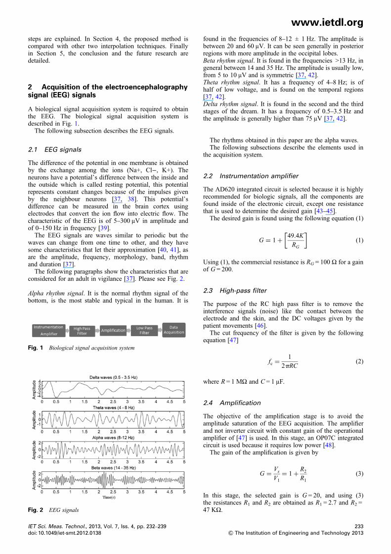
A biological signal acquisition system is required to obtainthe EEG. The biological signal acquisition system isdescribed in Fig. 1.The following subsection describes the EEG signals.

2.1 EEG signals

The difference of the potential in one membrane is obtainedby the exchange among the ions (Na+, Cl−, K+). Theneurons have a potential’s difference between the inside andthe outside which is called resting potential, this potentialrepresents constant changes because of the impulses givenby the neighbour neurons [37, 38]. This potential’sdifference can be measured in the brain cortex usingelectrodes that convert the ion flow into electric flow. Thecharacteristic of the EEG is of 5–300 μV in amplitude andof 0–150 Hz in frequency [39].The EEG signals are waves similar to periodic but the

waves can change from one time to other, and they havesome characteristics that let their approximation [40, 41], asare the amplitude, frequency, morphology, band, rhythmand duration [37].The following paragraphs show the characteristics that are

considered for an adult in vigilance [37]. Please see Fig. 2.

Alpha rhythm signal. It is the normal rhythm signal of thebottom, is the most stable and typical in the human. It is

Fig. 1 Biological signal acquisition system

Fig. 2 EEG signals

IET Sci. Meas. Technol., 2013, Vol. 7, Iss. 4, pp. 232–239doi: 10.1049/iet-smt.2012.0138

found in the frequencies of 8–12 ± 1 Hz. The amplitude isbetween 20 and 60 μV. It can be seen generally in posteriorregions with more amplitude in the occipital lobes.Beta rhythm signal. It is found in the frequencies >13 Hz, ingeneral between 14 and 35 Hz. The amplitude is usually low,from 5 to 10 μV and is symmetric [37, 42].Theta rhythm signal. It has a frequency of 4–8 Hz; is ofhalf of low voltage, and is found on the temporal regions[37, 42].Delta rhythm signal. It is found in the second and the thirdstages of the dream. It has a frequency of 0.5–3.5 Hz andthe amplitude is generally higher than 75 μV [37, 42].

The rhythms obtained in this paper are the alpha waves.The following subsections describe the elements used in

the acquisition system.

2.2 Instrumentation amplifier

The AD620 integrated circuit is selected because it is highlyrecommended for biologic signals, all the components arefound inside of the electronic circuit, except one resistancethat is used to determine the desired gain [43–45].The desired gain is found using the following equation (1)

G = 1+ 49.4K

RG

[ ](1)

Using (1), the commercial resistance is RG = 100 Ω for a gainof G = 200.

2.3 High-pass filter

The purpose of the RC high pass filter is to remove theinterference signals (noise) like the contact between theelectrode and the skin, and the DC voltages given by thepatient movements [46].The cut frequency of the filter is given by the following

equation [47]

fc =1

2pRC(2)

where R = 1 MΩ and C = 1 μF.

2.4 Amplification

The objective of the amplification stage is to avoid theamplitude saturation of the EEG acquisition. The amplifierand not inverter circuit with constant gain of the operationalamplifier of [47] is used. In this stage, an OP07C integratedcircuit is used because it requires low power [48].The gain of the amplification is given by

G = Vs

V1= 1+ R2

R1(3)

In this stage, the selected gain is G = 20, and using (3)the resistances R1 and R2 are obtained as R1 = 2.7 and R2 =47 KΩ.

233& The Institution of Engineering and Technology 2013

www.ietdl.org

2.5 Low-pass filter

In [49], it can be seen that if the order of the low-pass filterincreases, then also the slope and the filter behaviourincreases, the MAX7401 integrated circuit is used becauseit is an eight-order filter, which is recommended for lowerfrequencies [50].The cut frequency of the MAX7401 is given as follows

fosc(KHz) =k × 103

Cosc(4)

where k = 38, fosc = 100fc, and fc is the cut frequency.Using (4), Cosc is obtained as Cosc = 47 nF for a frequency

of fc = 15 Hz.

2.6 Final electronic circuit

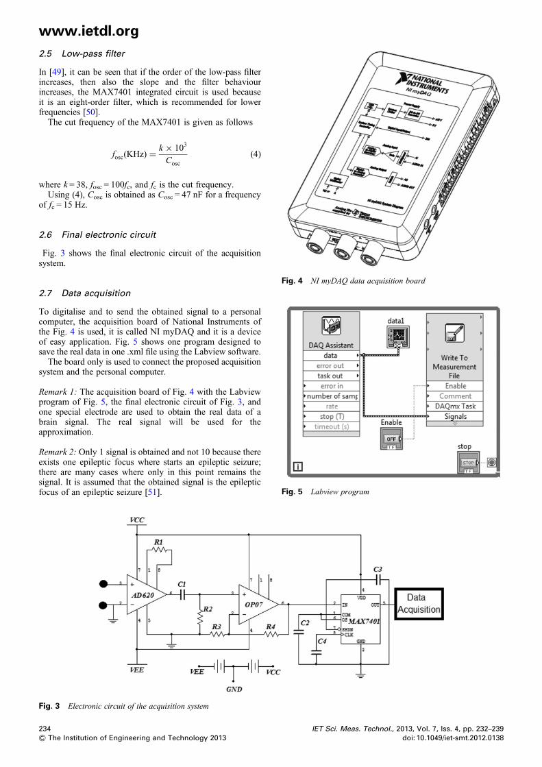
Fig. 3 shows the final electronic circuit of the acquisitionsystem.

Fig. 4 NI myDAQ data acquisition board

Fig. 5 Labview program

2.7 Data acquisition

To digitalise and to send the obtained signal to a personalcomputer, the acquisition board of National Instruments ofthe Fig. 4 is used, it is called NI myDAQ and it is a deviceof easy application. Fig. 5 shows one program designed tosave the real data in one .xml file using the Labview software.The board only is used to connect the proposed acquisition

system and the personal computer.

Remark 1: The acquisition board of Fig. 4 with the Labviewprogram of Fig. 5, the final electronic circuit of Fig. 3, andone special electrode are used to obtain the real data of abrain signal. The real signal will be used for theapproximation.

Remark 2: Only 1 signal is obtained and not 10 because thereexists one epileptic focus where starts an epileptic seizure;there are many cases where only in this point remains thesignal. It is assumed that the obtained signal is the epilepticfocus of an epileptic seizure [51].

Fig. 3 Electronic circuit of the acquisition system

234 IET Sci. Meas. Technol., 2013, Vol. 7, Iss. 4, pp. 232–239& The Institution of Engineering and Technology 2013 doi: 10.1049/iet-smt.2012.0138

www.ietdl.org

Remark 3: The real EEG signal is polluted with noise, thenoise is rejected with the filters constructed with the AD620integrated circuit of Fig. 3, and with a special electrode.

The following section presents the slopes algorithm.

3 Slopes algorithm

The slopes algorithm is described in this section.

3.1 Detailed description of the algorithm

Consider the function yk = f xk( )

[ < with xk [ <, for k =1, 2, …, T, T is the iterations number. The approximationconsists to find yk such that it approximates yk.The slope of yk denoted as mk using the xk and yk data of the

real brain signal is obtained as follows

mk =yk − yk−1

xk − xk−1(5)

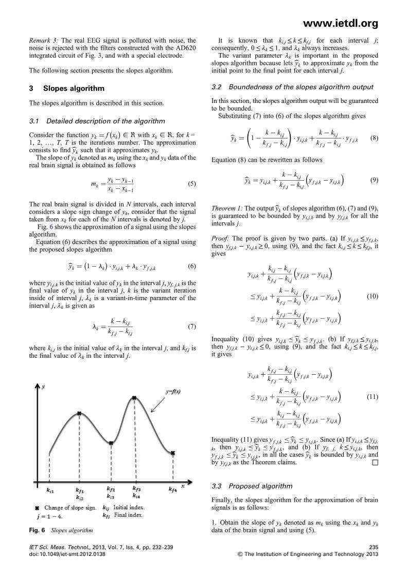
The real brain signal is divided in N intervals, each intervalconsiders a slope sign change of yk, consider that the signaltaken from xk for each of the N intervals is denoted by j.

Fig. 6 shows the approximation of a signal using the slopesalgorithm.Equation (6) describes the approximation of a signal using

the proposed slopes algorithm

yk = 1− lk( ) · yi,j,k + lk · y f ,j,k (6)

where yi,j,k is the initial value of yk in the interval j, yf, j,k is thefinal value of yk in the interval j, k is the variant iterationinside of interval j, λk is a variant-in-time parameter of theinterval j, λk is given as

lk =k − ki,jk f ,j − ki,j

(7)

where ki,j is the initial value of λk in the interval j, and kf,j isthe final value of λk in the interval j.

Fig. 6 Slopes algorithm

IET Sci. Meas. Technol., 2013, Vol. 7, Iss. 4, pp. 232–239doi: 10.1049/iet-smt.2012.0138

It is known that ki,j≤ k≤ kf,j for each interval j;consequently, 0≤ λk≤ 1, and λk always increases.The variant parameter λk is important in the proposed

slopes algorithm because lets yk to approximate yk from theinitial point to the final point for each interval j.

3.2 Boundedness of the slopes algorithm output

In this section, the slopes algorithm output will be guaranteedto be bounded.Substituting (7) into (6) of the slopes algorithm gives

yk = 1− k − ki,jk f ,j − ki,j

( )· yi,j,k +

k − ki,jk f ,j − ki,j

· y f ,j,k (8)

Equation (8) can be rewritten as follows

yk = yi,j,k +k − ki,jk f ,j − ki,j

y f ,j,k − yi,j,k

( )(9)

Theorem 1: The output yk of slopes algorithm (6), (7) and (9),is guaranteed to be bounded by yi,j,k and by yf,j,k for all theintervals j.

Proof: The proof is given by two parts. (a) If yi,j,k≤ yf,j,k,then yf,j,k − yi,j,k≥ 0, using (9), and the fact ki,j≤ k ≤ kf,j, itgives

yi,j,k +ki,j − ki,jk f ,j − ki,j

y f ,j,k − yi,j,k

( )≤ yi,j,k +

k − ki,jk f ,j − ki,j

y f ,j,k − yi,j,k

( )≤ yi,j,k +

k f ,j − ki,jk f ,j − ki,j

y f ,j,k − yi,j,k

( )(10)

Inequality (10) gives yi,j,k ≤ yk ≤ y f ,j,k . (b) If yf,j,k≤ yi,j,k,then yf,j,k − yi,j,k≤ 0, using (9), and the fact ki,j≤ k≤ kf,j,it gives

yi,j,k +k f ,j − ki,jk f ,j − ki,j

y f ,j,k − yi,j,k

( )≤ yi,j,k +

k − ki,jk f ,j − ki,j

y f ,j,k − yi,j,k

( )≤ yi,j,k +

ki,j − ki,jk f ,j − ki,j

y f ,j,k − yi,j,k

( )(11)

Inequality (11) gives y f ,j,k ≤ yk ≤ yi,j,k . Since (a) If yi,j,k≤ yf,j,k, then yi,j,k ≤ yk ≤ y f ,j,k , and (b) If yf, j, k≤ yi,j,k, theny f ,j,k ≤ yk ≤ yi,j,k , in all the cases yk is bounded by yi,j,k andby yf,j,k as the Theorem claims. □

3.3 Proposed algorithm

Finally, the slopes algorithm for the approximation of brainsignals is as follows:

1. Obtain the slope of yk denoted as mk using the xk and ykdata of the brain signal and using (5).

235& The Institution of Engineering and Technology 2013

www.ietdl.org

2. For each slope sign change of yk, obtain one intervaldenoted by j, the maximum number of intervals is N.3. For each interval j, obtain λk with (7).4. For each interval j, obtain yk as the approximation of ykusing (6).

4 Results and discussions

An acquisition system is used to obtain real data of two brainsignals. The acquisition system has an amplification of 4000and a cut frequency of 15 Hz. The acquisition system isapplied with a 28 years old healthy man with closed eyes,the electrode is localised in F3 because of the Internationalsystem 10–20. See Fig. 7, and references [52, 53]. Fig. 8shows the real acquisition system.The brain signals are obtained with the NI myDAQ that is

configured to obtain 1000 iterations per second. The firstbrain signal is obtained in one second from 5.5 to 6.5 s forthe example 1, and the second brain signal is obtained inone second from 150 to 151 s for the example 2.The slopes algorithm is compared with the least-squares

algorithm of [19, 22–32, 34], and with the nearestneighbour of [20, 21, 33] for the approximation of twobrain signals.

Fig. 7 Electrodes on the man

Fig. 8 Acquisition system

236& The Institution of Engineering and Technology 2013

To find the best algorithm, the root-mean-square error(RMSE) is used, it is described as follows [54–58]

RMSE = 1

T

∑Tk=1

e2i (k)

( )12

(12)

where T is the iterations number, and ei(k) = yk − yk is theapproximation error for each iteration.

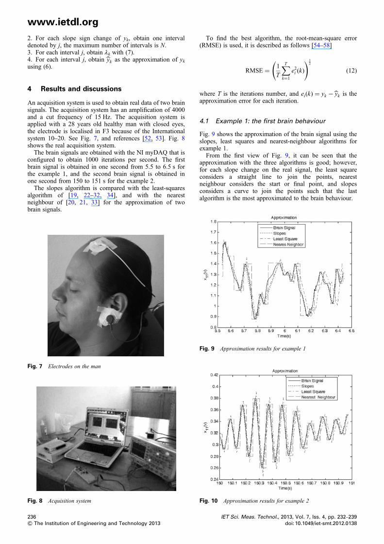
4.1 Example 1: the first brain behaviour

Fig. 9 shows the approximation of the brain signal using theslopes, least squares and nearest-neighbour algorithms forexample 1.From the first view of Fig. 9, it can be seen that the

approximation with the three algorithms is good; however,for each slope change on the real signal, the least squareconsiders a straight line to join the points, nearestneighbour considers the start or final point, and slopesconsiders a curve to join the points such that the lastalgorithm is the most approximated to the brain behaviour.

Fig. 9 Approximation results for example 1

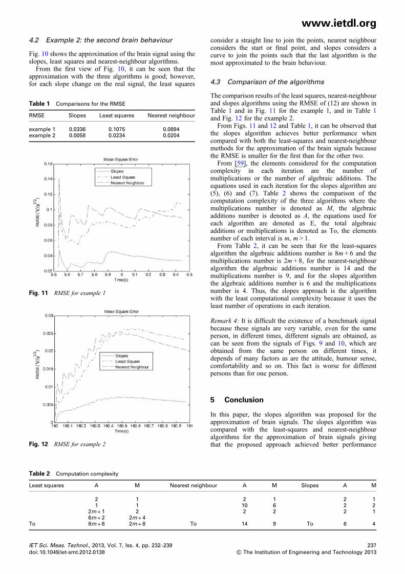
Fig. 10 Approximation results for example 2

IET Sci. Meas. Technol., 2013, Vol. 7, Iss. 4, pp. 232–239doi: 10.1049/iet-smt.2012.0138

www.ietdl.org

4.2 Example 2: the second brain behaviour

Fig. 10 shows the approximation of the brain signal using theslopes, least squares and nearest-neighbour algorithms.From the first view of Fig. 10, it can be seen that the

approximation with the three algorithms is good; however,for each slope change on the real signal, the least squares

Fig. 12 RMSE for example 2

Fig. 11 RMSE for example 1

Table 1 Comparisons for the RMSE

RMSE Slopes Least squares Nearest neighbour

example 1 0.0336 0.1075 0.0894example 2 0.0058 0.0234 0.0204

Table 2 Computation complexity

Least squares A M Nearest neighb

2 11 1

2m + 1 26m + 2 2m + 4

To 8m + 6 2m + 8 To

IET Sci. Meas. Technol., 2013, Vol. 7, Iss. 4, pp. 232–239doi: 10.1049/iet-smt.2012.0138

consider a straight line to join the points, nearest neighbourconsiders the start or final point, and slopes considers acurve to join the points such that the last algorithm is themost approximated to the brain behaviour.

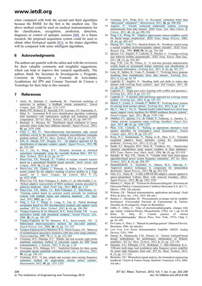
4.3 Comparison of the algorithms

The comparison results of the least squares, nearest-neighbourand slopes algorithms using the RMSE of (12) are shown inTable 1 and in Fig. 11 for the example 1, and in Table 1and Fig. 12 for the example 2.From Figs. 11 and 12 and Table 1, it can be observed that

the slopes algorithm achieves better performance whencompared with both the least-squares and nearest-neighbourmethods for the approximation of the brain signals becausethe RMSE is smaller for the first than for the other two.From [59], the elements considered for the computation

complexity in each iteration are the number ofmultiplications or the number of algebraic additions. Theequations used in each iteration for the slopes algorithm are(5), (6) and (7). Table 2 shows the comparison of thecomputation complexity of the three algorithms where themultiplications number is denoted as M, the algebraicadditions number is denoted as A, the equations used foreach algorithm are denoted as E, the total algebraicadditions or multiplications is denoted as To, the elementsnumber of each interval is m, m > 1.From Table 2, it can be seen that for the least-squares

algorithm the algebraic additions number is 8m + 6 and themultiplications number is 2m + 8, for the nearest-neighbouralgorithm the algebraic additions number is 14 and themultiplications number is 9, and for the slopes algorithmthe algebraic additions number is 6 and the multiplicationsnumber is 4. Thus, the slopes approach is the algorithmwith the least computational complexity because it uses theleast number of operations in each iteration.

Remark 4: It is difficult the existence of a benchmark signalbecause these signals are very variable, even for the sameperson, in different times, different signals are obtained, ascan be seen from the signals of Figs. 9 and 10, which areobtained from the same person on different times, itdepends of many factors as are the attitude, humour sense,comfortability and so on. This fact is worse for differentpersons than for one person.

5 Conclusion

In this paper, the slopes algorithm was proposed for theapproximation of brain signals. The slopes algorithm wascompared with the least-squares and nearest-neighbouralgorithms for the approximation of brain signals givingthat the proposed approach achieved better performance

our A M Slopes A M

2 1 2 110 6 2 22 2 2 1

14 9 To 6 4

237& The Institution of Engineering and Technology 2013

www.ietdl.org

when compared with both the second and third algorithmsbecause the RMSE for the first is the smallest one. Theabove method could be used on medical instrumentation forthe classification, recognition, prediction, detection,diagnosis or control of epileptic seizures [60]. As a futureresearch, the proposed acquisition system could be used toobtain other biological signals [61], or the slopes algorithmwill be compared with some intelligent algorithms.

6 Acknowledgments

The authors are grateful with the editor and with the reviewersfor their valuable comments and insightful suggestions,which can help to improve this research significantly. Theauthors thank the Secretara de Investigación y Posgrado,Comisión de Operación y Fomento de ActividadesAcadémicas del IPN and Consejo Nacional de Ciencia yTecnologa for their help in this research.

7 References

1 Amiri, M., Bahrami, F., Janahmadi, M.: ‘Functional modeling ofastrocytes in epilepsy: a feedback system perspective’, NeuralComput. Appl., 2011, 20, pp. 1131–1139

2 Barba, P.D., Komeza, K., Juszczak, E.N., Lecointe, J.P., Napieralski, P.,Hihat, N.: ‘Automated B–H curve identification algorithm combiningfield simulation with optimisation methods and exploiting parallelcomputation’, IET Sci. Meas. Technol., 2012, 6, (5), pp. 369–375

3 Bertrand, A., Moonen, M.: ‘Distributed signal estimation in sensornetworks where nodes have different interests’, Signal Process., 2012,92, pp. 1679–1690

4 Chen, C., Bro, O.: ‘Three-dimensional time-harmonic eddy currentproblems solved by the geometric multigrid preconditioned conjugategradient method’, IET Sci. Meas. Technol., 2012, 6, (5), pp. 319–323

5 Jelfs, B., Mandic, D.P., Douglas, S.C.: ‘An adaptive approach for theidentification of improper complex signals’, Signal Process., 2012, 92,pp. 335–344

6 Lei, J., Liu, S., Wang, X.Y.: ‘Dynamic inversion in electricalcapacitance tomography using the ensemble Kalman filter’, IET Sci.Meas. Technol., 2012, 6, (2), pp. 63–77

7 Pérez-Cruz, J.H., Poznyak, A.: ‘Control of nuclear research reactorsbased on a generalized Hopfield neural network’, Intell. Autom. SoftComput., 2010, 16, (1), pp. 39–60

8 Pérez-Cruz, J.H., Chairez, I., Poznyak, A., Rubio, J.J.: ‘Constrainedneural control for the adaptive tracking of power profiles in a Trigareactor’, Int. J. Innov. Comput., Inf. Control, 2011, 7, (7),pp. 4575–4788

9 Pérez Cruz, J.H., Ruiz Velázquez, E., Rubio, J.J., de Alba Padilla, C.A.:‘Robust adaptive neurocontrol of SISO nonlinear systems preceded byunknown deadzone’, Math. Probl. Eng., 2012, 2012, pp. 1–23

10 Pérez-Cruz, J.H., Rubio, J.J., Ruiz-Velázquez, E., Sols-Perales, G.:‘Tracking control based on recurrent neural networks for nonlinearsystems with multiple inputs and unknown deadzone’, Abs. Appl.Anal., 2012, 2012, pp. 1–18

11 Tang, J., Liu, F., Zhang, X., Liang, X., Fan, Q.: ‘Partial dischargerecognition based on SF6 decomposition products and support vectormachine’, IET Sci. Meas. Technol., 2012, 6, (4), pp. 198–204

12 Vazquez-Espinosa de los Monteros, R.A., Sossa-Azuela, J.H.: ‘A newassociative model with dynamical synapses’, Neural Process. Lett.,2008, 28, (3), pp. 189–207

13 Vazquez-Espinosa de los Monteros, R.A., Sossa-Azuela, J.H.: ‘Abidirectional hetero-associative memory for true-color patterns’,Neural Process. Lett., 2008, 28, (3), pp. 131–153

14 Vazquez-Espinosa de los Monteros, R.A., Sossa-Azuela, J.H.: ‘Behaviorof morphological associative memories with true-color image patterns’,Neurocomputing, 2009, 73, (1–3), pp. 225–244

15 Vizireanu, D.N., Halunga, S.V.: ‘Simple, fast and accurate eight pointsamplitude estimation method of sinusoidal signals for DSP basedinstrumentation’, J. Instrum., 2012, 7, (4), pp. 1–10

16 Vizireanua, D.N., Halunga, S.V.: ‘Analytical formula for three pointssinusoidal signals amplitude estimation errors’, Int. J. Electron., 2012,99, (1), pp. 149–151

17 Vizireanu, D.N.: ‘A fast, simple and accurate time-varying frequencyestimation method for single-phase electric power systems’,Measurement, 2012, 45, pp. 1331–1333

238& The Institution of Engineering and Technology 2013

18 Vizireanu, D.N., Preda, R.O.: ‘Is “five-point” estimation better than“three-point” estimation?’, Measurement, 2013, 46, pp. 840–842

19 Angelov, P.: ‘Fuzzily connected multimodel systems evolvingautonomously from data streams’, IEEE Trans. Syst. Man Cybern. B,Cybern., 2011, 41, (4), pp. 898–910

20 Tong, C.S., Wong, M.: ‘Adaptive approximate nearest neighbor searchfor fractal image compression’, IEEE Trans. Image Process., 2002,11, (6), pp. 605–615

21 Dening, D.C., Gray, F.G., Haralick Robert, M.: ‘Prosthesis control usinga nearest neighbor electromyographic pattern classifier’, IEEE Trans.Biomed. Eng., 1983, BME-30, (6), pp. 356–360

22 Iglesias, J.A., Angelov, P., Ledezma, A., Sanchis, A.: ‘Creating evolvinguser behavior profiles automatically’, IEEE Trans. Knowl. Data Eng.,2011, 24, (5), pp. 854–867

23 Jang, Y.M., Lee, M., Ozawa, S.: ‘A real-time personal authenticationsystem based on incremental feature extraction and classification ofaudiovisual information’, Evolving Syst., 2011, 2, (4), pp. 261–272

24 Leite, D., Ballini, R., Costa, P., Gomide, F.: ‘Evolving fuzzy granularmodeling from nonstationary fuzzy data streams’, Evolving Syst.,2012, 3, (2), pp. 65–79

25 Lughofer, E., Angelov, P.: ‘Handling drifts and shifts in online datastreams with evolving fuzzy systems’, Appl. Soft Comput., 2011, 11,(2), pp. 2057–2068

26 Lughofer, E.: ‘Single pass active learning with conflict and ignorance’,Evolving Syst., 2012, 3, pp. 251–271

27 Lughofer, E.: ‘A dynamic split-and-merge approach for evolving clustermodels’, Evolving Syst., 2012, 3, pp. 135–151

28 Maciel, L., Lemos, A., Gomide, F., Ballini, R.: ‘Evolving fuzzy systemsfor pricing fixed income options’, Evolving Syst., 2012, 3, pp. 5–18

29 Mu, C., Sun, C., Yu, X.: ‘Internal model control based on a novel leastsquare support vector machines for MIMO nonlinear discrete systems’,Neural Comput. Appl., 2011, 20, pp. 1159–1166

30 Ordóñez, F.J., Iglesias, J.A., de Toledo, P., Ledezma, A., Sanchis, A.:‘Online activity recognition using evolving classifiers’, Expert Syst.Appl., 2013, 40, (4), pp. 1248–1255

31 Phan, A.H., Cichocki, A.: ‘Seeking an appropriate alternative leastsquares algorithm for nonnegative tensor factorizations’, NeuralComput. Appl., 2012, 21, pp. 623–637

32 Rong, H.-J., Sundararajan, N., Huang, G.-B., Zhao, G.-S.: ‘Extendedsequential adaptive fuzzy inference system for classificationproblems’, Evolving Syst., 2011, 2, (2), pp. 71–82

33 Smith, S.J., Bourgoin, M.O., Sims, K., Voorhees, H.L.: ‘Handwrittencharacter classification using nearest neighbor in large databases’,IEEE Trans. Pattern Anal. Mach. Intell., 1994, 16, (9), pp. 915–919

34 Subudhi, B., Ray, P.K., Ghosh, S.: ‘Variable leaky least mean-squarealgorithm-based power system frequency estimation’, IET Sci. Meas.Technol., 2012, 6, (4), pp. 288–297

35 ParandehGheibi, A., Ayremlou, A., Akhaee, M.A., Marvasti, F.:‘Improved iterative techniques to compensate for interpolationdistortions’, Signal Process., 2012, 92, pp. 963–976

36 Ortiz, E.L., Seara, R.: ‘A fully LMS/NLMS adaptive scheme applied tosparse-interpolated Volterra filters with removed boundary effect’,Signal Process., 2012, 92, pp. 2381–2393

37 Martnez, C., Rojas, B.: ‘Técnicas de electroencefalografa’ (Secretaria deEducación Pública, Comunicaciones Cientficas Mexicanas S.A. de C.V.,México, 1998, 2da edición)

38 Webster, J.B.: ‘Medical instrumentation, applicattion and design’ (JonhWiley & Sons, Inc., USA, 2010, 4th edn.)

39 Ramrez, C., Hernández, M.: ‘Procesamiento en tiempo real de variablesfisiológicas’ (Universidad Nacional de Experimental de Táchira,Decanato de Investigación, Grupo de Biomédica)

40 Gibbs, F., Gibbs, E.: ‘Atlas of electroencephalography, changes whitage, asleep’ (Addison-Wesley, Massachusetts, 1950), vol. 1, pp. 82–89

41 Klass, D., Daly, D.: ‘Current practice of clinicalelectroencephalography’ (Raven Press, New York, 1975), Chap 5,pp. 69–109

42 De Castro, S., Pérez, J.: ‘Manual de patologa general’ (Masson/Elsevier,Barcelona, 2006, 6ta edición)

43 Low Cost, Low Power Instrumentation Amplifier AD620, AnalogDevices, USA, 1999

44 Darraji, R., Ghannouchi, F.M., Hammi, O.: ‘Generic load-pull-baseddesign methodology for performance optimisation of Dohertyamplifiers’, IET Sci. Meas. Technol., 2012, 6, (3), pp. 132–138

45 Hussaini, A.S., Elfergani, I.T.E., Rodriguez, J., Abd-Alhameed, R.A.:‘Efficient multi-stage load modulation radio frequency power amplifierfor green radio frequency front end’, IET Sci. Meas. Technol., 2012,6, (3), pp. 117–124

46 Bronzino, J.D.: ‘Biomedical signal analysis, the biomedical engineeringhandbook’ (Taylor & Francis Group, Hartford, Conneticut, USA, 2006,3rd edn.)

IET Sci. Meas. Technol., 2013, Vol. 7, Iss. 4, pp. 232–239doi: 10.1049/iet-smt.2012.0138

www.ietdl.org

47 Boylestad, R.L., Nashelsky, L.: ‘Electronic devices and circuit theory’

(Prentice-Hall, 2008, 10th edn.)48 Ultralow Offset Voltage Operational Amplifier, OP07, Analog Devices49 Rubio, J.J., Vazquez, D., Pacheco, J., Garcia, V.: ‘Mathematical model

of low pass filters’, Recent Patents Eng., 2011, 5, (2), pp. 155–16250 8th-Order, Lowpass, Bessel, Switched-Capacitor Filters, Max7401,

Maxim, USA, 199951 Gutiérrez, J.: ‘Detección del foco epiléptico y su ruta de propagación’.

Congreso Latinoamericano de Ingeniera Boimédica, 200152 Homan, R.: ‘Cerebral location of international 10–20 system electrode

placement’, Electroencephalogr. Clin. Neurophysiol., 1987, 66,pp. 376–382

53 Jasper, H.: ‘The ten-twenty electrode system of the internationalfederation, recommendations for the practice of clinicalneurophysiology’ (The International Federation Societies forElectroencephalography and Clinical Neurophysiology, Elsevier,Amsterdam, 1983), pp. 3–10

54 Rubio, J.J., Angelov, P., Pacheco, J.: ‘An uniformly stablebackpropagation algorithm to train a feedforward neural network’,IEEE Trans. Neural Netw., 2011, 22, (3), pp. 356–366

IET Sci. Meas. Technol., 2013, Vol. 7, Iss. 4, pp. 232–239doi: 10.1049/iet-smt.2012.0138

55 Rubio, J.J., Garca, E., Pacheco, J.: ‘Trajectory planning and collisionsdetector for robotic arms’, Neural Comput. Appl., 2012, 21, (8),pp. 2105–2114

56 Rubio, J.J.: ‘Modified optimal control with a backpropagation network forRobotic arms’, IET Control Theory Appl., 2012, 6, (14), pp. 2216–2225

57 Rubio, J.J., Figueroa, M., Perez-Cruz, J.H., Bejarano, F.J.: ‘Geometricapproach and structure at infinite controls for the disturbancerejection’, IET Control Theory Appl., 2012, 6, (16), pp. 2528–2537

58 Rubio, J.J., Figueroa, M., Pérez-Cruz, J.H., Rumbo, J.: ‘Control tostabilize and mitigate disturbances in a rotary inverted pendulum’,Mex. J. Phys. E, 2012, 58, (2), pp. 107–112

59 Khalil, W., Kleinfinger, J., Gautier, M.: ‘Reducing the computationalburden of the dynamic models of robots’, IEEE Int. Conf. Robot.Autom., 1986, 3, pp. 525–531

60 Bairagi, V.K., Sapkal, A.M.: ‘Automated region-based hybridcompression for digital imaging and communications in medicinemagnetic resonance imaging images for telemedicine applications’,IET Sci. Meas. Technol., 2012, 6, (4), pp. 247–253

61 Rubio, J.J., Ortiz, F., Mariaca, C.R., Tovar, J.C.: ‘A method for onlinepattern recognition for abnormal eye movements’, Neural Comput.Appl., 2013, 22, (3–4), pp. 597–605

239& The Institution of Engineering and Technology 2013