Accounting and Statistical Analyses for Sustainable ... - OAPEN
288
Sustainable Management, Wertschöpfung und Effizienz Accounting and Statistical Analyses for Sustainable Development Multiple Perspectives and Information-Theoretic Complexity Reduction Claudia Lemke
-
Upload
khangminh22 -
Category
Documents
-
view
2 -
download
0
Transcript of Accounting and Statistical Analyses for Sustainable ... - OAPEN

Sustainable Management, Wertschöpfung und Effizienz
Accounting and Statistical Analyses for Sustainable Development Multiple Perspectives and Information-Theoretic Complexity Reduction
Claudia Lemke

Sustainable Management,Wertschopfung und Effizienz
Series Editors
Gregor Weber, Breunigweiler, Germany
Markus Bodemann, Warburg, Germany
René Schmidpeter, Köln, Germany

In dieser Schriftenreihe stehen insbesondere empirische und praxisnahe Studienzu nachhaltigem Wirtschaften und Effizienz im Mittelpunkt. Energie-, Umwelt-,Nachhaltigkeits-, CSR-, Innovations-, Risiko- und integrierte Managementsys-teme sind nur einige Beispiele, die Sie hier wiederfinden. Ein besonderer Fokusliegt dabei auf dem Nutzen, den solche Systeme für die Anwendung in der Pra-xis bieten, um zu helfen die globalen Nachhaltigkeitsziele (SDGs) umzusetzen.Publiziert werden nationale und internationale wissenschaftliche Arbeiten.
Reihenherausgeber:Dr. Gregor Weber, ecoistics.instituteDr. Markus BodemannProf. Dr. René Schmidpeter, Center for Advanced Sustainable Management,Cologne Business School
This series is focusing on empirical and practical research in the fields of sustaina-ble management and efficiency. Management systems in the context of energy,environment, sustainability, CSR, innovation, risk as well as integrated manage-ment systems are just a few examples which can be found here. A special focus ison the value such systems can offer for the application in practice supporting theimplementation of the global sustainable development goals, the SDGs. Nationaland international scientific publications are published (English and German).
Series Editors:Dr. Gregor Weber, ecoistics.instituteDr. Markus BodemannProf. Dr. René Schmidpeter, Center for Advanced Sustainable Management,Cologne Business School
More information about this series at http://www.springer.com/series/15909

Claudia Lemke
Accounting andStatistical Analysesfor SustainableDevelopmentMultiple Perspectives andInformation-Theoretic ComplexityReduction

Claudia LemkeBerlin, Germany
Dissertation Technische Universität Berlin, 2020
ISSN 2523-8620 ISSN 2523-8639 (electronic)Sustainable Management, Wertschöpfung und EffizienzISBN 978-3-658-33245-7 ISBN 978-3-658-33246-4 (eBook)https://doi.org/10.1007/978-3-658-33246-4
© The Editor(s) (if applicable) and The Author(s). This book is an open access publication. 2021Open Access This book is licensed under the terms of the Creative Commons Attribution 4.0International License (http://creativecommons.org/licenses/by/4.0/), which permits use, sharing,adaptation, distribution and reproduction in any medium or format, as long as you give appropriatecredit to the original author(s) and the source, provide a link to the Creative Commons license andindicate if changes were made.The images or other third party material in this book are included in the book’s Creative Commonslicense, unless indicated otherwise in a credit line to the material. If material is not included in thebook’s Creative Commons license and your intended use is not permitted by statutory regulation orexceeds the permitted use, you will need to obtain permission directly from the copyright holder.The use of general descriptive names, registered names, trademarks, service marks, etc. in thispublication does not imply, even in the absence of a specific statement, that such names are exemptfrom the relevant protective laws and regulations and therefore free for general use.The publisher, the authors and the editors are safe to assume that the advice and information in thisbook are believed to be true and accurate at the date of publication. Neither the publisher nor theauthors or the editors give a warranty, expressed or implied, with respect to the material containedherein or for any errors or omissions that may have been made. The publisher remains neutral withregard to jurisdictional claims in published maps and institutional affiliations.
Planung/Lektorat: Carina ReiboldThis Springer Gabler imprint is published by the registered company Springer FachmedienWiesbaden GmbH part of Springer Nature.The registered company address is: Abraham-Lincoln-Str. 46, 65189 Wiesbaden, Germany

Preface
Claudia Lemke’s dissertation addresses the aim to develop a sustainable development
indicator set that
1. includes the economic, environmental, and social domains and maps their interre-
lations into a composite measure;
2. incorporates the so-called “multilevel perspective”, i.e. it is applicable to economic
units of different size; and
3. overcomes critical conceptual and methodological deficiencies identified in index
construction for sustainable development.
To meet this objective, Claudia Lemke derives a profound conceptual framework
of sustainable development. Theoretical principles for the assessment of contributions
to sustainable development are outlined and an overview of assessment methodologies
is provided. Because the thesis identifies indicator sets and composite indicators (i.e.
indices) derived from them as an expedient method to meet conceptual requirements
and assessment principles, the methodology of a novel index, the Multilevel Sustainable
Development Index (MLSDI), is derived subsequently.
Weighting and aggregation are crucial steps in index construction. In terms of weight-
ing, the thesis identifies statistical procedures as expedient to yield the most promising
results, because they are able to account for the correlations of underlying variables
from the environmental, economic, and social domains. Three specific techniques are
identified and tested against each other: Principal Component Analysis (PCA), Partial
Triadic Analysis (PTA), and the information-theoretic Maximum Relevance Minimum
Redundancy Backward (MRMRB) algorithm. For aggregation purposes, geometric
aggregation is identified as the only method that accounts for non-comparable and
ratio-scaled indicators.
The methodology is applied to a sample of the German economy for the years 2008
to 2016 in the empirical part of the dissertation. A comparable assessment of different
branches is performed within each of the three domains and the aggregated MLSDI is
derived for selected branches of the German economy.
This work has far-reaching implications for research and practice. With regards
to sustainable development research, major contributions include the inclusion of the
v
vi Preface
multilevel perspective. A wide range of indicators from all three domains of sustainable
development are integrated and the analysis of their interconnections is performed in
the statistical procedure of the innovative MRMRB algorithm. The thesis further uses
open source data and makes all methodological choices transparent. Its Implications
for practice include the support of policy-level decisions, because a methodologically
sound and comparable tool is proposed to assess the sustainability performances of
different units of account. The MLSDI is further proposed as an alternative to the Gross
Domestic Product (GDP) as a measure of societal wellbeing at the policy level, because
economic growth is limited and the additional dimensions of environmental protection
and social development need to be considered when assessing societal wellbeing.
Claudia Lemke’s dissertation therefore represents an important contribution to the
research field of how a comparable evaluation of sustainability performances of units
of different size can be performed. The results are equally important for science and
practice. I wish Claudia Lemke’s work the attention it certainly deserves.
Berlin, July 2020 JProf. Dr. Karola Bastini

Foreword
After submitting her dissertation to Technische Universitat Berlin, Claudia Lemke
joined the Beiersdorf AG as a Supply Chain Sustainability Manager. Since 1882, the
name Beiersdorf stands for innovative skin care. We continuously develop our products
and brands to win consumers’ loyalty and trust through best-in-class quality. Nowadays,
quality and trust do not only refer to the use phase of a product, but the consumers of
today – and even more the consumers of tomorrow – demand products with a reduced
environmental impact as well as an increased value for society. Innovative value creation
goes beyond improving the consumer’s experience of product application. Sustainable
production and consumption are one of the great challenges of the 21st century, and
especially global corporations have to take on the responsibility to contribute to societal
wellbeing by taking the entire value chain and life cycle of their products into account.
Beiersdorf meets the needs of these increased demands and has publicly pledged to
improve its environmental footprint and social impact at global level.
Beiersdorf quantifies its sustainable development performances according to the
Global Reporting Initiative (GRI) and allocates its contributions to the Sustainable
Development Goals (SDGs). These two guiding frameworks are the foundation of
Claudia Lemke’s dissertation. By aligning the corporate GRI framework and the
societal SDG framework at indicator level, Claudia Lemke enables the measurement of
corporate contributions to societal sustainable development. Moreover, by developing
a methodologically sound sustainable development index from this newly aligned
indicator base, Claudia Lemke facilitates benchmarking throughout all aspects of
sustainable development. Benchmarking in turn facilitates decision making in modern-
day corporations, often dealing with several competing priorities.
By co-funding the open access publication of Claudia Lemke’s dissertation, Beiersdorf
supports the public accessibility of this excellent theoretical and methodological research.
Knowledge and education should not be exclusive, but inclusiveness is part of sustainable
development and Beiersdorf’s vision. We are proud to care beyond skin.
Hamburg, November 2020 Jean-Francois PascalVice President SustainabilityBeiersdorf AG
vii

Acknowledgement
The present dissertation was developed during my occupation as a (senior) research
associate at the economic research institute WifOR and later in the Field of Sustainability
Accounting and Management Control at the Technische Universitat Berlin under the
supervision of JProf. Dr. Karola Bastini. This dissertation is submitted to acquire
the academic degree of Doctor of Business and Economic Sciences (Dr. rer. oec.) at
the Technische Universitat Berlin. Parts of the dissertation are published in Lemke
and Bastini (2020). I state my deepest recognition to everyone who has supported me
during my time as a doctoral student.
First, I am grateful to JProf. Dr. Karola Bastini for her supervision and far-reaching
feedback. Her eager willingness and engaged passion for scientific debates contributed
considerably to the successful completion of my dissertation project. I also thank Prof.
Dr. Maik Lachmann, Chair of Accounting and Management Control at the Technische
Universitat Berlin, for being the secondary referee of my dissertation.
I am grateful to Prof. Dr. Dennis A. Ostwald for supporting my dissertation project
during my tenure at WifOR with his stimulating visions and encouraging leadership. I
am also thankful for fruitful methodological debates with Dr. Marcus Cramer. I thank
Rita Bergmann for her secondary authorships of the first two working papers of my
dissertation project as well as her strengthening joy and ease in life. I appreciate the
permission to include data on the German health economy by Jochen Puth-Weissenfels,
Federal Ministry for Economic Affairs and Energy (BMWi).
Furthermore, I thank Fares Getzin for exchanging valuable thoughts and mutual
motivations on progresses of our dissertations throughout my time at the Technische
Universitat Berlin. I also appreciate the fruitful debates and the motivating moments
with all other colleagues at the Technische Universitat Berlin and WifOR.
Last but foremost, I thank my partner Alexander Andor for never-ending encourage-
ment, tolerance, and patience in both good and bad times of my dissertation. I am also
thankful to my friend Cordula Klaus for her long-lasting support and cheering spirits. I
am grateful to my parents Soon Boon and Bernd Lemke as well as my sister Susanne
Lemke for providing a network of safety throughout all ups and downs of my entire
academic career.
Berlin, February 2020 Claudia Lemke
ix
x Acknowledgement
To Clea and all future generations to come
The publication of this work was funded by the Open Access Publication Fund of
Technische Universitat Berlin and the Beiersdorf AG.

Table of contents
Preface v
Foreword vii
Acknowledgement ix
Table of contents xi
List of abbreviations xv
List of figures xix
List of tables xxiii
List of equations xxvii
List of symbols xxix
1 Introduction 1
1.1 Background and motivation . . . . . . . . . . . . . . . . . . . . . . . . 1
1.2 Research question and aim of the dissertation . . . . . . . . . . . . . . 4
1.3 Procedure . . . . . . . . . . . . . . . . . . . . . . . . . . . . . . . . . . 6
2 Conceptual framework of sustainable development 9
2.1 Definition of sustainable development and sustainability . . . . . . . . . 10
2.2 The three contentual domains of sustainable development . . . . . . . . 13
2.2.1 Environmental protection . . . . . . . . . . . . . . . . . . . . . 13
2.2.2 Social development . . . . . . . . . . . . . . . . . . . . . . . . . 15
2.2.3 Economic prosperity . . . . . . . . . . . . . . . . . . . . . . . . 18
2.2.4 Integration of the three contentual domains . . . . . . . . . . . 20
2.3 Stakeholders and change agents of sustainable development . . . . . . . 24
2.3.1 The multilevel perspective . . . . . . . . . . . . . . . . . . . . . 25
2.3.2 Corporate sustainability . . . . . . . . . . . . . . . . . . . . . . 26
2.3.3 Political goal setting: The United Nations’s (UN) Sustainable
Development Goals (SDGs) . . . . . . . . . . . . . . . . . . . . 32
xi

xii Table of contents
2.3.4 Sustainability science . . . . . . . . . . . . . . . . . . . . . . . . 36
2.4 Summary . . . . . . . . . . . . . . . . . . . . . . . . . . . . . . . . . . 38
3 Measuring and assessing contributions to sustainable development 41
3.1 Principles of sustainable development measurement and assessment methods 43
3.2 Overview of quantitative sustainable development assessment methods 46
3.3 Sustainable development indicators . . . . . . . . . . . . . . . . . . . . 52
3.3.1 Corporate indicator frameworks . . . . . . . . . . . . . . . . . . 53
3.3.2 Meso-level indices . . . . . . . . . . . . . . . . . . . . . . . . . . 54
3.3.3 Macro-level indices . . . . . . . . . . . . . . . . . . . . . . . . . 55
3.4 Summary . . . . . . . . . . . . . . . . . . . . . . . . . . . . . . . . . . 60
4 Methodology 63
4.1 Overview of sustainable development indices’ calculation steps and meth-
odological requirements . . . . . . . . . . . . . . . . . . . . . . . . . . . 64
4.2 Methodological evaluation of sustainable development indices . . . . . . 67
4.3 Methodology of the Multilevel Sustainable Development Index (MLSDI) 72
4.3.1 Collection of sustainable development key figures . . . . . . . . 72
4.3.2 Preparation of sustainable development key figures . . . . . . . 74
4.3.2.1 Meso-level transformation to macro-economic categories 74
4.3.2.2 Macro-level transformation of statistical classifications 74
4.3.3 Imputation of missing values . . . . . . . . . . . . . . . . . . . . 76
4.3.3.1 Characterisation of missing values . . . . . . . . . . . . 77
4.3.3.2 Single time series imputation: Various methods depend-
ing on the missing data pattern . . . . . . . . . . . . . 78
4.3.3.3 Multiple panel data imputation: Amelia II algorithm . 80
4.3.3.4 Statistical tests of model assumptions . . . . . . . . . 82
4.3.4 Standardisation to sustainable development key indicators . . . 84
4.3.5 Outlier detection and treatment . . . . . . . . . . . . . . . . . . 88
4.3.5.1 Characterisation of outliers . . . . . . . . . . . . . . . 89
4.3.5.2 Univariate Interquartile Range (IQR) method . . . . . 89
4.3.6 Scaling . . . . . . . . . . . . . . . . . . . . . . . . . . . . . . . . 91
4.3.6.1 Characterisation of scales . . . . . . . . . . . . . . . . 92
4.3.6.2 Rescaling between ten and 100 . . . . . . . . . . . . . 93
4.3.7 Weighting . . . . . . . . . . . . . . . . . . . . . . . . . . . . . . 95
4.3.7.1 Overview of weighting methods . . . . . . . . . . . . . 96
4.3.7.2 Multivariate statistical analysis: Principal Component
Analysis (PCA) . . . . . . . . . . . . . . . . . . . . . . 98
4.3.7.3 Multivariate statistical analysis: Partial Triadic Ana-
lysis (PTA) . . . . . . . . . . . . . . . . . . . . . . . . 100

Table of contents xiii
4.3.7.4 Information theory: Maximum Relevance Minimum
Redundancy Backward (MRMRB) algorithm . . . . . 101
4.3.7.5 Statistical tests of model assumptions . . . . . . . . . 103
4.3.8 Aggregation . . . . . . . . . . . . . . . . . . . . . . . . . . . . . 104
4.3.9 Sensitivity analyses . . . . . . . . . . . . . . . . . . . . . . . . . 106
4.4 Summary and interim conclusion . . . . . . . . . . . . . . . . . . . . . 107
5 Empirical findings 113
5.1 Data base, objects of investigation, and time periods . . . . . . . . . . 114
5.2 Sustainable development key figures . . . . . . . . . . . . . . . . . . . . 116
5.2.1 Collection and preparation of sustainable development key figures 117
5.2.2 Imputation of missing values . . . . . . . . . . . . . . . . . . . . 121
5.3 Sustainable development key indicators . . . . . . . . . . . . . . . . . . 126
5.3.1 Alignment of the Global Reporting Initiative (GRI) and the
Sustainable Development Goal (SDG) disclosures . . . . . . . . 127
5.3.1.1 Environmental sustainable development key indicators 127
5.3.1.2 Social sustainable development key indicators . . . . . 130
5.3.1.3 Economic sustainable development key indicators . . . 133
5.3.2 Summary statistics of the sustainable development growth indicators136
5.3.3 Outlier detection and treatment . . . . . . . . . . . . . . . . . . 139
5.3.4 Empirical findings of the cleaned and rescaled sustainable devel-
opment key indicators . . . . . . . . . . . . . . . . . . . . . . . 140
5.3.4.1 Summary statistics . . . . . . . . . . . . . . . . . . . . 141
5.3.4.2 Comparative analysis of the selected branches . . . . . 153
5.4 Weighting . . . . . . . . . . . . . . . . . . . . . . . . . . . . . . . . . . 158
5.4.1 The Principal Component (PC) family’s eigenvalues and explained
cumulative variances . . . . . . . . . . . . . . . . . . . . . . . . 158
5.4.2 The Maximum Relevance Minimum Redundancy Backward
(MRMRB) algorithm’s discretisation and backward elimination . 160
5.4.3 Comparative analysis of weights . . . . . . . . . . . . . . . . . . 160
5.4.4 Statistical tests of the Principal Component (PC) family . . . . 166
5.5 Empirical findings of the four composite sustainable development measures168
5.5.1 Summary statistics . . . . . . . . . . . . . . . . . . . . . . . . . 168
5.5.2 Comparative analysis of the selected branches . . . . . . . . . . 171
5.6 Sensitivity analyses . . . . . . . . . . . . . . . . . . . . . . . . . . . . . 175
5.7 Summary . . . . . . . . . . . . . . . . . . . . . . . . . . . . . . . . . . 178
6 Discussion and conclusion 181
6.1 Implications for research . . . . . . . . . . . . . . . . . . . . . . . . . . 181
6.2 Implications for practice . . . . . . . . . . . . . . . . . . . . . . . . . . 184
xiv Table of contents
6.3 Limitations and future outlook . . . . . . . . . . . . . . . . . . . . . . 186
6.4 Summary and conclusion . . . . . . . . . . . . . . . . . . . . . . . . . . 190
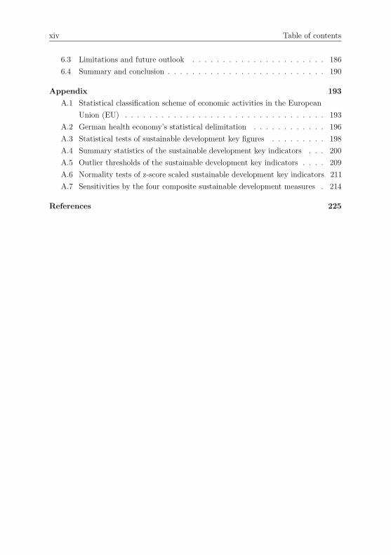
Appendix 193
A.1 Statistical classification scheme of economic activities in the European
Union (EU) . . . . . . . . . . . . . . . . . . . . . . . . . . . . . . . . . 193
A.2 German health economy’s statistical delimitation . . . . . . . . . . . . 196
A.3 Statistical tests of sustainable development key figures . . . . . . . . . 198
A.4 Summary statistics of the sustainable development key indicators . . . 200
A.5 Outlier thresholds of the sustainable development key indicators . . . . 209
A.6 Normality tests of z-score scaled sustainable development key indicators 211
A.7 Sensitivities by the four composite sustainable development measures . 214
References 225

List of abbreviations
A4S Prince’s Accounting for Sustainability Project
aHC average Headcount
AIChE American Institute of Chemical Engineers
ARIMA Autoregressive Integrated Moving Average
BA Federal Employment Agency
Bellagio STAMP Bellagio Sustainability Assessment and Measurement Principles
BLI Better Life Index
BMJV Federal Ministry of Justice and Consumer Protection
BMWi Federal Ministry for Economic Affairs and Energy
CBS Centre for Bhutan Studies
CEFIC European Chemical Industry Council
CEPI Composite Environmental Performance Index
CIS Compass Index of Sustainability
CIT Corporate Income Tax
CO2 Carbon Dioxide
CO2e Carbon Dioxide Equivalents
CPA Classification of Products by Activity
CRAN Comprehensive R Archive Network
Destatis Federal Bureau of Statistics
DJSI Dow Jones Sustainability Indices
EC European Commission
EDP Eco Domestic Product
EEA European Environment Agency
EPI Environmental Performance Index
ESA European System of Accounts
xv
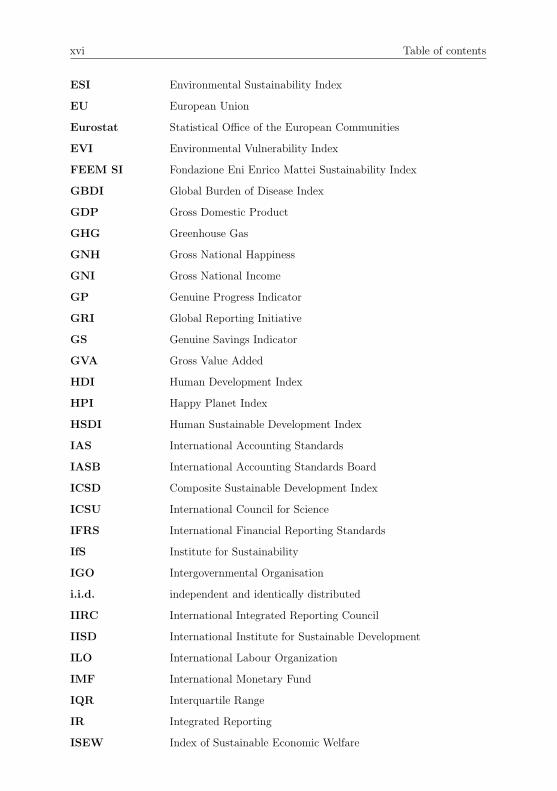
xvi Table of contents
ESI Environmental Sustainability Index
EU European Union
Eurostat Statistical Office of the European Communities
EVI Environmental Vulnerability Index
FEEM SI Fondazione Eni Enrico Mattei Sustainability Index
GBDI Global Burden of Disease Index
GDP Gross Domestic Product
GHG Greenhouse Gas
GNH Gross National Happiness
GNI Gross National Income
GP Genuine Progress Indicator
GRI Global Reporting Initiative
GS Genuine Savings Indicator
GVA Gross Value Added
HDI Human Development Index
HPI Happy Planet Index
HSDI Human Sustainable Development Index
IAS International Accounting Standards
IASB International Accounting Standards Board
ICSD Composite Sustainable Development Index
ICSU International Council for Science
IFRS International Financial Reporting Standards
IfS Institute for Sustainability
IGO Intergovernmental Organisation
i.i.d. independent and identically distributed
IIRC International Integrated Reporting Council
IISD International Institute for Sustainable Development
ILO International Labour Organization
IMF International Monetary Fund
IQR Interquartile Range
IR Integrated Reporting
ISEW Index of Sustainable Economic Welfare

Table of contents xvii
ISO International Organization for Standardization
ISSC International Social Science Council
IT Information Technology
IW Inclusive Wealth Index
KMO Kaiser-Meyer-Olkin
LPI Living Planet Index
MAR Missing at Random
MCAR Missing Completely at Random
MDG Millennium Development Goal
MISD Mega Index of Sustainable Development
MLSDI Multilevel Sustainable Development Index
MNAR Missing Not at Random
MRMRB Maximum Relevance Minimum Redundancy Backward
n/a not applicable
NACE Statistical Classification of Economic Activities in the EuropeanCommunity
NEF New Economic Foundation
NDP Net Domestic Product
NNI Net National Income
OAT One-at-a-Time
OECD Organisation for Economic Co-operation and Development
p.c. per capita
PC Principal Component
PCA Principal Component Analysis
p.h. per hour
PTA Partial Triadic Analysis
R&D Research and Development
SASB Sustainability Accounting Standards Boards
SDG Sustainable Development Goal
SDGI Sustainable Development Goal Index
SDI Sustainable Development Index
SNBI Sustainable Net Benefit Index
SSI Sustainable Society Index
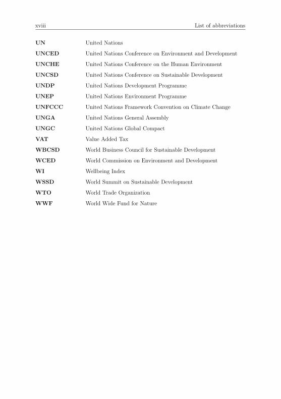
xviii List of abbreviations
UN United Nations
UNCED United Nations Conference on Environment and Development
UNCHE United Nations Conference on the Human Environment
UNCSD United Nations Conference on Sustainable Development
UNDP United Nations Development Programme
UNEP United Nations Environment Programme
UNFCCC United Nations Framework Convention on Climate Change
UNGA United Nations General Assembly
UNGC United Nations Global Compact
VAT Value Added Tax
WBCSD World Business Council for Sustainable Development
WCED World Commission on Environment and Development
WI Wellbeing Index
WSSD World Summit on Sustainable Development
WTO World Trade Organization
WWF World Wide Fund for Nature

List of figures
Figure 2.1 The first two dimensions of the sustainable development space . . . 11
Figure 2.2 The first three dimensions of the sustainable development space . . 12
Figure 2.3 Nine planetary boundaries and current statuses of exploitation . . . 15
Figure 2.4 Maslow’s hierarchy of needs and the principle of justice . . . . . . . 17
Figure 2.5 12 social boundaries and current statuses of achievement . . . . . . 18
Figure 2.6 Relationship of the three contentual domains . . . . . . . . . . . . 22
Figure 2.7 The safe and just operating space for humanity . . . . . . . . . . . 23
Figure 2.8 Venn and concentric diagrams of weak and strong sustainability . . 24
Figure 2.9 The first four dimensions of the sustainable development space . . . 25
Figure 2.10 The first five dimensions of the sustainable development space . . . 27
Figure 2.11 The six-dimensional sustainable development space and the threeconceptual principles of its management . . . . . . . . . . . . . . . 29
Figure 2.12 The Sustainable Development Goals (SDGs) . . . . . . . . . . . . . 34
Figure 2.13 Conceptual agenda of a transdisciplinary research processes . . . . 37
Figure 3.1 Overview of sustainable development assessment methods by theaggregational size of an object of investigation . . . . . . . . . . . . 47
Figure 3.2 Capability evaluation of assessment principle compliance by indicatorsets and footprints . . . . . . . . . . . . . . . . . . . . . . . . . . . 51
Figure 3.3 Evaluation of assessment principle compliance by meso-level indicesof sustainable development . . . . . . . . . . . . . . . . . . . . . . 54
Figure 3.4 Overview of Gross Domestic Product (GDP) alternatives . . . . . . 57
Figure 3.5 Evaluation of assessment principle compliance by macro-level indicesof sustainable development . . . . . . . . . . . . . . . . . . . . . . 58
Figure 3.6 Ranking of sustainable development indices by assessment principlecompliance . . . . . . . . . . . . . . . . . . . . . . . . . . . . . . . 60
Figure 4.1 Calculation steps of a sustainable development index . . . . . . . . 65
Figure 4.2 Layers of an overall sustainable development index . . . . . . . . . 66
Figure 4.3 Evaluation of methodological soundness and linkage to assessmentprinciples by meso-level indices of sustainable development . . . . . 68
xix

xx List of figures
Figure 4.4 Evaluation of methodological soundness and linkage to assessmentprinciples by macro-level indices of sustainable development . . . . 70
Figure 4.5 Structure of the sustainable development key figures’ data set . . . 73
Figure 4.6 Examples of missing data patterns . . . . . . . . . . . . . . . . . . 78
Figure 4.7 Spectrum from normal data to strong outliers . . . . . . . . . . . . 89
Figure 5.1 Missing data pattern in the German economy in 2008 . . . . . . . . 122
Figure 5.2 Missing data pattern in the German economy in 2013 . . . . . . . . 123
Figure 5.3 Single time series imputation on import in billion Euro for the selectedbranches in the German economy from 2008 to 2016 . . . . . . . . 124
Figure 5.4 Multiple imputation on import in billion Euro for the selectedbranches in the German economy from 2008 to 2016 . . . . . . . . 125
Figure 5.5 Frequency distribution of import and air emissions in the Germaneconomy in 2016 . . . . . . . . . . . . . . . . . . . . . . . . . . . . 126
Figure 5.6 Convergence of the Amelia II algorithm with overdispersed startvalues for the largest Principal Component (PC) . . . . . . . . . . 127
Figure 5.7 Outliers of the air emissions intensity in gram Carbon Dioxide Equi-valents (CO2e) in the German economy from 2008 to 2016 . . . . . 139
Figure 5.8 Outliers of the share of imported input in percentage of input in theGerman economy from 2008 to 2016 . . . . . . . . . . . . . . . . . 140
Figure 5.9 Environmental ratio indicators in rescaled performance scores for theselected branches in the German economy in 2016 . . . . . . . . . . 154
Figure 5.10 Environmental growth indicators in rescaled performance scores forthe selected branches in the German economy . . . . . . . . . . . . 155
Figure 5.11 Social ratio indicators in rescaled performance scores for the selectedbranches in the German economy in 2016 . . . . . . . . . . . . . . 156
Figure 5.12 Social and economic growth indicators in rescaled performance scoresfor the selected branches in the German economy . . . . . . . . . . 157
Figure 5.13 Economic ratio indicators in rescaled performance scores for theselected branches in the German economy in 2016 . . . . . . . . . . 158
Figure 5.14 Eigenvalues and explained cumulative variances of the PrincipalComponent Analysis (PCA) and the Partial Triadic Analysis (PTA) 159
Figure 5.15 Importance factors of the Principal Component Analysis (PCA),Partial Triadic Analysis (PTA), and the Maximum Relevance Min-imum Redundancy Backward (MRMRB) algorithm . . . . . . . . . 167
Figure 5.16 The four composite measures in rescaled performance scores in theGerman economy from 2008 to 2016 . . . . . . . . . . . . . . . . . 171
Figure 5.17 Frequency distribution and density of the four composite measuresin the German economy in 2016 . . . . . . . . . . . . . . . . . . . . 171
Figure 5.18 Environmental subindex in rescaled performance scores for the selec-ted branches in the German economy from 2008 to 2016 . . . . . . 172

List of figures xxi
Figure 5.19 Social subindex in rescaled performance scores for the selectedbranches in the German economy from 2008 to 2016 . . . . . . . . 173
Figure 5.20 Economic subindex in rescaled performance scores for the selectedbranches in the German economy from 2008 to 2016 . . . . . . . . 174
Figure 5.21 Overall Multilevel Sustainable Development Index (MLSDI) in res-caled performance scores for the selected branches in the Germaneconomy from 2008 to 2016 . . . . . . . . . . . . . . . . . . . . . . 174
Figure 5.22 The four composite measures by the three outlier detection methodsin rescaled performance scores in the German economy in 2016 . . 176
Figure 5.23 The four composite measures by the three weighting methods inrescaled performance scores in the German economy in 2016 . . . . 177
Figure A.1 Frequency distribution of z-score scaled average compensation ofemployees per capita (p.c.) and consumed capital productivity in theGerman economy in 2016 . . . . . . . . . . . . . . . . . . . . . . . 213
Figure A.2 Frequency distribution by the four composite measures and thethree outlier detection methods in rescaled performance scores in theGerman economy in 2016 . . . . . . . . . . . . . . . . . . . . . . . 218
Figure A.3 Frequency distribution of the four composite measures by the threeweighting methods in rescaled performance scores in the Germaneconomy in 2016 . . . . . . . . . . . . . . . . . . . . . . . . . . . . 223
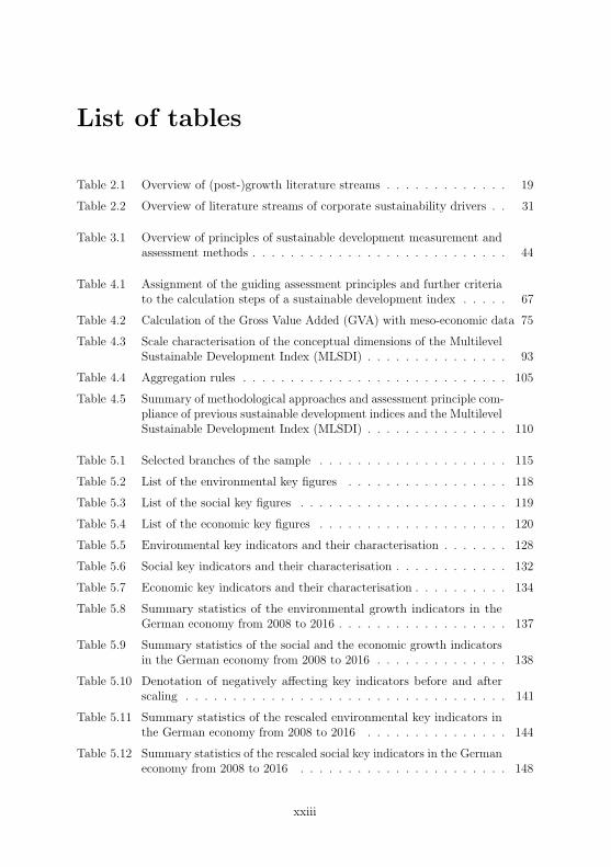
List of tables
Table 2.1 Overview of (post-)growth literature streams . . . . . . . . . . . . . 19
Table 2.2 Overview of literature streams of corporate sustainability drivers . . 31
Table 3.1 Overview of principles of sustainable development measurement andassessment methods . . . . . . . . . . . . . . . . . . . . . . . . . . . 44
Table 4.1 Assignment of the guiding assessment principles and further criteriato the calculation steps of a sustainable development index . . . . . 67
Table 4.2 Calculation of the Gross Value Added (GVA) with meso-economic data 75
Table 4.3 Scale characterisation of the conceptual dimensions of the MultilevelSustainable Development Index (MLSDI) . . . . . . . . . . . . . . . 93
Table 4.4 Aggregation rules . . . . . . . . . . . . . . . . . . . . . . . . . . . . 105
Table 4.5 Summary of methodological approaches and assessment principle com-pliance of previous sustainable development indices and the MultilevelSustainable Development Index (MLSDI) . . . . . . . . . . . . . . . 110
Table 5.1 Selected branches of the sample . . . . . . . . . . . . . . . . . . . . 115
Table 5.2 List of the environmental key figures . . . . . . . . . . . . . . . . . 118
Table 5.3 List of the social key figures . . . . . . . . . . . . . . . . . . . . . . 119
Table 5.4 List of the economic key figures . . . . . . . . . . . . . . . . . . . . 120
Table 5.5 Environmental key indicators and their characterisation . . . . . . . 128
Table 5.6 Social key indicators and their characterisation . . . . . . . . . . . . 132
Table 5.7 Economic key indicators and their characterisation . . . . . . . . . . 134
Table 5.8 Summary statistics of the environmental growth indicators in theGerman economy from 2008 to 2016 . . . . . . . . . . . . . . . . . . 137
Table 5.9 Summary statistics of the social and the economic growth indicatorsin the German economy from 2008 to 2016 . . . . . . . . . . . . . . 138
Table 5.10 Denotation of negatively affecting key indicators before and afterscaling . . . . . . . . . . . . . . . . . . . . . . . . . . . . . . . . . . 141
Table 5.11 Summary statistics of the rescaled environmental key indicators inthe German economy from 2008 to 2016 . . . . . . . . . . . . . . . 144
Table 5.12 Summary statistics of the rescaled social key indicators in the Germaneconomy from 2008 to 2016 . . . . . . . . . . . . . . . . . . . . . . 148
xxiii

xxiv List of tables
Table 5.13 Summary statistics of the rescaled economic key indicators in theGerman economy from 2008 to 2016 . . . . . . . . . . . . . . . . . . 152
Table 5.14 Rescaled key indicators’ ranking according to the backward elim-ination of the Maximum Relevance Minimum Redundancy Back-ward (MRMRB) algorithm . . . . . . . . . . . . . . . . . . . . . . . 161
Table 5.15 Environmental key indicators’ weights derived by the Principal Com-ponent Analysis (PCA), Partial Triadic Analysis (PTA), and theMaximum Relevance Minimum Redundancy Backward (MRMRB)algorithm . . . . . . . . . . . . . . . . . . . . . . . . . . . . . . . . 162
Table 5.16 Social key indicators’ weights derived by the Principal ComponentAnalysis (PCA), Partial Triadic Analysis (PTA), and the MaximumRelevance Minimum Redundancy Backward (MRMRB) algorithm . 164
Table 5.17 Economic key indicators’ weights derived by the Principal ComponentAnalysis (PCA), Partial Triadic Analysis (PTA), and the MaximumRelevance Minimum Redundancy Backward (MRMRB) algorithm . 165
Table 5.18 Summary statistics of the subindices and the overall Multilevel Sus-tainable Development Index (MLSDI) in the German economy from2008 to 2016 . . . . . . . . . . . . . . . . . . . . . . . . . . . . . . . 169
Table 5.19 Average rank shifts of economic objects by the four composite meas-ures and the three outlier and weighting methods in 2016 . . . . . . 175
Table A.1 Sections and divisions in the German economy according to theStatistical Classification of Economic Activities in the EuropeanCommunity (NACE) . . . . . . . . . . . . . . . . . . . . . . . . . . 196
Table A.2 German health economy’s stakes in divisions at two-digit level inpercentage from 2008 to 2016 . . . . . . . . . . . . . . . . . . . . . 198
Table A.3 Environmental key figures’ test statistics and p-values of the Shapiro-Wilk (SW), Kolmogorov-Smirnov (KS), augmented Dickey-Fuller(aDF), and the Ljung-Box (LB) tests . . . . . . . . . . . . . . . . . 198
Table A.4 Social key figures’ test statistics and p-values of the Shapiro-Wilk(SW), Kolmogorov-Smirnov (KS), augmented Dickey-Fuller (aDF),and the Ljung-Box (LB) tests . . . . . . . . . . . . . . . . . . . . . 199
Table A.5 Economic key figures’ test statistics and p-values of the Shapiro-Wilk(SW), Kolmogorov-Smirnov (KS), augmented Dickey-Fuller (aDF),and the Ljung-Box (LB) tests . . . . . . . . . . . . . . . . . . . . . 200
Table A.6 Summary statistics of the environmental key indicators in the Germaneconomy from 2008 to 2016 . . . . . . . . . . . . . . . . . . . . . . 202
Table A.7 Summary statistics of the social key indicators in the German economyfrom 2008 to 2016 . . . . . . . . . . . . . . . . . . . . . . . . . . . . 205
Table A.8 Summary statistics of the economic key indicators in the Germaneconomy from 2008 to 2016 . . . . . . . . . . . . . . . . . . . . . . 209
Table A.9 Environmental key indicators’ upper and lower outlier thresholds . . 209
Table A.10 Social key indicators’ upper and lower outlier thresholds . . . . . . 210

List of tables xxv
Table A.11 Economic key indicators’ upper and lower outlier thresholds . . . . 211
Table A.12 Z-score scaled environmental key indicators’ average test statisticsand p-values of the Shapiro-Wilk (SW) and the Kolmogorov-Smirnov(KS) tests from 2008 to 2016 . . . . . . . . . . . . . . . . . . . . . . 211
Table A.13 Z-score scaled social key indicators’ average test statistics and p-values of the Shapiro-Wilk (SW) and the Kolmogorov-Smirnov (KS)tests from 2008 to 2016 . . . . . . . . . . . . . . . . . . . . . . . . . 212
Table A.14 Z-score scaled economic key indicators’ average test statistics andp-values of the Shapiro-Wilk (SW) and the Kolmogorov-Smirnov (KS)tests from 2008 to 2016 . . . . . . . . . . . . . . . . . . . . . . . . . 213
Table A.15 Ranking of the economic objects in Statistical Classification of Eco-nomic Activities in the European Community (NACE) codes by thefour composite measures and the three outlier detection methods inthe German economy in 2016 . . . . . . . . . . . . . . . . . . . . . 217
Table A.16 Ranking of the economic objects in Statistical Classification of Eco-nomic Activities in the European Community (NACE) codes by thefour composite measures and the three weighting methods in theGerman economy in 2016 . . . . . . . . . . . . . . . . . . . . . . . . 222

List of equations
Equation 4.1 Set of sustainable development key figures . . . . . . . . . . . . . 72
Equation 4.2 Technology matrix for transformation of statistical classifications 76
Equation 4.3 Transformation of statistical classifications from Classificationof Products by Activity (CPA) to Statistical Classification ofEconomic Activities in the European Community (NACE) . . . . 76
Equation 4.4 Set of sustainable development key figures in Statistical Classifica-tion of Economic Activities in the European Community (NACE) 76
Equation 4.5 Basic structural time series model . . . . . . . . . . . . . . . . . 79
Equation 4.6 Relative efficiency in convergence of an estimate in multiple im-putation . . . . . . . . . . . . . . . . . . . . . . . . . . . . . . . 80
Equation 4.7 Set of sustainable development key indicators . . . . . . . . . . . 85
Equation 4.8 Sustainable development ratio indicator . . . . . . . . . . . . . . 87
Equation 4.9 Sustainable development growth indicator . . . . . . . . . . . . . 87
Equation 4.10 Thresholds for outlying sustainable development key indicators . 90
Equation 4.11 Interquartile Range (IQR) measure . . . . . . . . . . . . . . . . . 90
Equation 4.12 Outlying sustainable development key indicator . . . . . . . . . . 91
Equation 4.13 Rescaling of a sustainable development key indicator . . . . . . . 95
Equation 4.14 Set of rescaled sustainable development key indicators . . . . . . 95
Equation 4.15 Weight of a sustainable development key indicator derived by thePrincipal Component Analysis (PCA) . . . . . . . . . . . . . . . 99
Equation 4.16 Importance factor of a sustainable development key indicatorderived by the Principal Component Analysis (PCA) . . . . . . . 99
Equation 4.17 Set of sustainable development key components . . . . . . . . . . 100
Equation 4.18 Weight of a time period derived by the Partial Triadic Analysis (PTA)100
Equation 4.19 Weight of a sustainable development key indicator derived by thePartial Triadic Analysis (PTA) . . . . . . . . . . . . . . . . . . . 100
Equation 4.20 Importance factor of a sustainable development key indicatorderived by the Partial Triadic Analysis (PTA) . . . . . . . . . . . 101
Equation 4.21 Bin size of equal frequency discretisation for the Maximum Relev-ance Minimum Redundancy Backward (MRMRB) algorithm . . . 103
Equation 4.22 Number of bins of equal frequency discretisation for the MaximumRelevance Minimum Redundancy Backward (MRMRB) algorithm 103
xxvii

xxviii List of equations
Equation 4.23 Weight of a sustainable development key indicator derived by theMaximum Relevance Minimum Redundancy Backward (MRMRB)algorithm . . . . . . . . . . . . . . . . . . . . . . . . . . . . . . . 103
Equation 4.24 Importance factor of a sustainable development key indicatorderived by the Maximum Relevance Minimum Redundancy Back-ward (MRMRB) . . . . . . . . . . . . . . . . . . . . . . . . . . . 103
Equation 4.25 Weighted product to compute a subindex of a contentual domain 106
Equation 4.26 Set of the sustainable development subindices . . . . . . . . . . . 106
Equation 4.27 Geometric mean to compute the overall Multilevel SustainableDevelopment Index (MLSDI) . . . . . . . . . . . . . . . . . . . . 106

List of symbols
α Outlier coefficient
β Outlier rate
c1 Overall Multilevel Sustainable Development Index (MLSDI)
c2 Set of sustainable development subindices
c3 Set of sustainable development key components
c4 Set of sustainable development key indicators
c4s Set of rescaled sustainable development key indicators
c5 Set of sustainable development key figures
cNACE5 Set of sustainable development key figures in Statistical Classification of
Economic Activities in the European Community (NACE)
χn Number of bins of equal frequency discretisation for the Maximum RelevanceMinimum Redundancy Backward (MRMRB) algorithm
χs Bin size of equal frequency discretisation for the Maximum RelevanceMinimum Redundancy Backward (MRMRB) algorithm
d Subindex of a contentual domain
D Number of subindices
δmax Maximum of the rescaling range
δmin Minimum of the rescaling range
ε Random noise in a basic structural time series model
η Relative efficiency in convergence of an estimate in multiple imputation
γ Seasonal component in a basic structural time series model
I Identity matrix
λ Rate of missing values
m Number of imputations in multiple imputation
MT Technology matrix
μ Trend component in a basic structural time series model
xxix

xxx List of equations
n Economic object
N Number of economic objects
ω Weight of a sustainable development key indicator
ωMRMRB Weight of a sustainable development key indicator derived by the MaximumRelevance Minimum Redundancy Backward (MRMRB) algorithm
ωPC Weights of a sustainable development key indicator derived by the PrincipalComponent (PC) family
ωPCA Weight of a sustainable development key indicator derived by the PrincipalComponent Analysis (PCA)
ωPCAt Weight of a sustainable development key indicator derived by the Principal
Component Analysis (PCA) in a time period
ωPTA Weight of a sustainable development key indicator derived by the PartialTriadic Analysis (PTA)
ΩPTA Weight of a time period derived by the Partial Triadic Analysis (PTA)
p Sustainable development key component
P Number of sustainable development key components
ψ Importance factor of a sustainable development key indicator
ψMRMRB Importance factor of a sustainable development key indicator derived by theMaximum Relevance Minimum Redundancy Backward (MRMRB) algorithm
ψPC Importance factor of a sustainable development key indicator derived by thePrincipal Component (PC) family
ψPCA Importance factor of a sustainable development key indicator derived by thePrincipal Component Analysis (PCA)
ψPTA Importance factor of a sustainable development key indicator derived by thePartial Triadic Analysis (PTA)
q Interquartile Range (IQR)
Q1 25th percentile of a distribution
Q3 75th percentile of a distribution
r Geographical region
R Number of geographical regions
S Supply table
t Time period
T Number of time periods
θ Outlier thresholds
θmax Upper outlier threshold

List of symbols xxxi
θmin Lower outlier threshold
x Sustainable development key figure
xCPA Sustainable development key figure in Classification of Products byActivity (CPA)
xNACE Sustainable development key figure in Statistical Classification of EconomicActivities in the European Community (NACE)
xstd Standardising sustainable development key figure
X Number of sustainable development key figures
ξ Effective direction of a sustainable development key indicator
ξ+ Positive effective direction of a sustainable development key indicator
ξ− Negative effective direction of a sustainable development key indicator
y Sustainable development key indicator
yg Sustainable development growth indicator
ygs Rescaled sustainable development growth indicator
ymax Maximum of a sustainable development key indicator in the sample
ymin Minimum of a sustainable development key indicator in the sample
yo Outlying sustainable development key indicator
yr Sustainable development ratio indicator
yrs Rescaled sustainable development ratio indicator
ys Rescaled sustainable development key indicator
yz Z-score scaled sustainable development key indicator
Y Number of sustainable development key indicators
Yg Number of sustainable development growth indicators
Ygs Number of rescaled sustainable development growth indicators
Yo Number of outlying sustainable development key indicators
Yr Number of sustainable development ratio indicators
Yrs Number of rescaled sustainable development ratio indicators
Ys Number of rescaled sustainable development key indicators
Yz Number of z-score scaled sustainable development key indicators

Chapter 1
Introduction
“The world has enough for everyone’s need, but not enough for everyone’s greed.”
Mohandas K. Gandhi
1.1 Background and motivation
The Atlantic hurricane season terminated for this term with category-5 hurricanes
such as Dorian (National Weather Service, 2019). Because of climate change, intense
and damaging hurricanes are three times more frequent nowadays than 100 years ago
(Grinsted, Ditlevsen & Hesselbjerg, 2019; McGrath, 2019). Likewise, scientific evidence
suggests that climate change made Europe’s major heatwave in 2018 more than twice
as likely to occur (Schiermeier, 2018; World Weather Attribution, 2018). Less dominant
in public but at higher and more alarming risk than climate change is the genetic
biodiversity of the biosphere (Steffen et al., 2015). Extinction rates may be 100 to
1,000 times higher than corresponding natural background rates (Ceballos et al., 2015;
de Vos, Joppa, Gittleman, Stephens & Pimm, 2015). These examples demonstrate the
abandonment of the Holocene and the entering of the Anthropocene, a new geological
era that is characterised by threatening human activities towards fundamental Earth
system dynamics (e.g. Griggs et al., 2013; Rockstrom et al., 2009b; Sachs, 2012). In
addition to that, humanitarian crises persist. The number of people living in extreme
poverty is declining, but projections estimate that 479 million people will remain in
extreme poverty in 2030 (Roser & Ortiz-Ospina, 2019) – 479 million people too many.
Sustainable development and sustainability consist of three contentual domains:
environmental protection, social development, and economic prosperity. Today’s and
tomorrow’s human needs should be satisfied subject to respecting present and future
environmental limits (Holden, Linnerud & Banister, 2017; WCED, 1987). Economic
prosperity serves this purpose (UNCED, 1992). Traditionally, the satisfaction of needs is
enabled by economic growth at the expense of the environment and social justice (A. B.
Atkinson, 2015; Holden et al., 2017; Piketty, 2014). Decoupling the nexus of economic
© The Author(s) 2021C. Lemke, Accounting and Statistical Analyses for SustainableDevelopment, Sustainable Management, Wertschöpfung undEffizienz, https://doi.org/10.1007/978-3-658-33246-4_1
2 Chapter 1. Introduction
growth and environmental degradation or social deprivation is a current challenge for
decision makers (Holden, Linnerud & Banister, 2014). Human-nature interactions in a
complex socio-ecological system (Clark, van Kerkhoft, Lebel & Gallopın, 2016; Hall,
Feldpausch-Parker, Peterson, Stephens & Wilson, 2017; WCED, 1987) are studied
in sustainability science, with the objective to develop a solution-oriented agenda
(Kates, 2015) for sustainable development and sustainability. Generally, sustainable
development and sustainability are characterised by complexity, which might be held
liable for our unsustainable world. From an economic theory perspective, unsustainable
outcomes are present due to market failures. Environmental and social externalities are
not internalised (Patterson, McDonald & Hardy, 2017; Sala, Ciuffo & Nijkamp, 2015),
and governmental regulation is demanded for correction. At the moment, sustainable
development and sustainability are visions of future (White, 2013), and the goal is to
turn the sustainable future into the present as soon as possible. Pursuing this goal
is widely referred to be the major and the most difficult challenge of today’s society
(van Poeck, Læssøe & Block, 2017).
To take up the challenge of making our world environmentally and socially sus-
tainable, measurement and assessment of sustainable development performances are
inevitable. Only what is measured can be managed (e.g. Parris & Kates, 2003). Indic-
ator sets are central for sustainable development measurement because they are able
to capture complexity: Indicator sets can cover a wide range of aspects of the three
contentual domains (Almassy & Pinter, 2018), multiple objects of investigations, large
time series, and diverse geographical regions. Including an index or a composite measure
in an indicator set yields further advantages. An index is a compressed description of
a multidimensional state (Ebert & Welsch, 2004) and hence reduces complexity (Bell
& Morse, 2018). The important focus in measurement is recaptured (Griggs et al.,
2014), combating the disadvantage of a rich indicator set to potentially cause more
confusion than understanding (Wu & Wu, 2012). Several scholars even argue that a
sustainable development index is necessarily required because such complexity cannot
be mapped by standalone indicators (Almassy & Pinter, 2018; Costanza, Fioramonti
& Kubiszewski, 2016; Hanley, Moffatt, Faichney & Wilson, 1999; Nardo et al., 2008;
Ramos & Moreno Pires, 2013). Moreover, sustainable development indices have the
potential to replace the Gross Domestic Product (GDP) as a measure of societal well-
being (Costanza, Fioramonti & Kubiszewski, 2016; Costanza et al., 2014). GDP has
been heavily criticised for being an insufficient measure of wellbeing because it only
quantifies the size of an economy in terms of final goods and services (Costanza et al.,
2014; Giannetti, Agostinho, Villas Boas de Almeida & Huisingh, 2015; van den Bergh,
2009). In contrast, sustainable development indices are metrics that fulfil the ambitions
of measures of wellbeing as they comprehensively describe environmental, social, and
economic aspects. A further major advantage of sustainable development indices is
their capability to explore interactions of individual sustainable development elements
1.1. Background and motivation 3
(Costanza, Fioramonti & Kubiszewski, 2016; T. Hahn & Figge, 2011). Knowledge
about these interactions are prerequisites for the effectiveness of coordinated actions
and thus for maximising progress on sustainable development (Costanza, Fioramonti
& Kubiszewski, 2016; ICSU & ISSC, 2015; Spaiser, Ranganathan, Swain & Sumpter,
2017; Weitz, Carlsen, Nilsson & Skanberg, 2018).
Several weaknesses and gaps are present in the field of sustainable development
indicators and indices, which motivate this research. First, conceptual frameworks of
sustainable development lack multiple perspectives (e.g. Baumgartner, 2014; Boron
& Murray, 2004; Chofreh & Goni, 2017; Griggs et al., 2014; Maletic, Maletic, Dahl-
gaard, Dahlgaard-Park & Gomiscek, 2014), such that previous sustainable development
indicators and indices can only be applied to economic objects of the same aggrega-
tional size. However, a comparable multilevel assessment of economic objects of any
aggregational size is crucial because sustainable development is a society level concept
(T. Hahn, Pinkse, Preuss & Figge, 2015; Jennings & Zandbergen, 1995), and effects on
the planet (macro level) are the cumulative results of individuals (micro level) (Dahl,
2012). Sustainable development and sustainability can only be achieved if micro and
meso objects contribute (Griggs et al., 2014; Sachs, 2012). A positive side effect of
this mandatory requirement of multilevel comparability is the provision of objective
macro-economic benchmarks that prevent meso-economic objects such as corporations
from greenwashing their sustainable development performances. The micro-to-macro
connection is seen as the major challenge that scholars from business and economics
face (McGregor & Pouw, 2017). The management literature calls for a meso-to-macro
connection in order to stop missing the “big picture” (Whiteman, Walker & Perego,
2013). To the best of the author’s knowledge, multilevel indicators and indices that ad-
dress this perspective gap by being comparably applicable to micro (individuals), meso
(organisations such as corporations), and macro objects (conglomerates of organisations
such as industries or overall economies) are absent in the academic literature. This
work is motivated by this call and will make significant contributions to this challenge.
Second, sustainable development and sustainability is mostly integrated at operational
tiers while lacking strategic and normative tiers (Baumgartner & Rauter, 2017; Tseng,
Lim & Wu, 2018). This operational-to-normative gap is a further reason for deficiencies
in the progress towards sustainability. The conceptual part of this work will address
the operational-to-normative gap. Third, a knowledge gap on interactions of individual
sustainable development elements is present (see above), and generating insights about
synergies and trade-offs of individual sustainable development elements is a subject of
current research (e.g. Allen, Metternicht & Wiedmann, 2019; Nilsson, Griggs & Visback,
2016; Pradhan, Costa, Rybski, Lucht & Kropp, 2017; Spaiser et al., 2017; Weitz et al.,
2018). This work is motivated by the knowledge gap and will contribute new meth-
odological and empirical understandings. Fourth, bottlenecks in the science-practice
linkage persist (Agyeman, 2005; Christie & Warburton, 2001; Hall et al., 2017; Sala,
4 Chapter 1. Introduction
Farioli & Zamagni, 2013), further harming the progress towards sustainability. The
empirical part of this work will contribute to this knowledge-to-action or sustainab-
ility gap. Fifth and last, previous sustainable development indices such as the Dow
Jones Sustainability Indices (DJSI) (e.g. RobecoSAM, 2018a), Composite Sustainable
Development Index (ICSD) (Krajnc & Glavic, 2005), Sustainable Development Goal
Index (SDGI) (e.g. Schmidt-Traub, Kroll, Teksoz, Durand-Delacre & Sachs, 2017a),
or the Sustainable Society Index (SSI) (e.g. van de Kerk, Manuel & Kleinjans, 2014)
feature methodological shortcomings, such that decisions based on these metrics may be
misled (Bohringer & Jochem, 2007; Mayer, 2008). This study is motivated by making
methodological contributions to the (sustainable development) index literature.
The following section, Section 1.2, explains how the present work will take up these
challenges and fill the five identified research gaps, setting the research question and
aim of this dissertation.
1.2 Research question and aim of the dissertation
Against this background, the present dissertation aspires to contribute to the science
and practice community to accelerate progress in sustainable development. In doing so,
it addresses the call that sustainable development demands performance measurement
by an indicator set that includes a composite measure to replace GDP as a measure of
wellbeing (see Section 1.1; e.g. Costanza, Fioramonti & Kubiszewski, 2016). It further
acknowledges that multiple perspectives must be comparably captured (see Section 1.1;
e.g. Dahl, 2012) in a methodologically sound manner to avoid misled decision making
(see Section 1.1; e.g. Bohringer & Jochem, 2007). As multilevel sustainable development
indices are not represented in the literature (see Section 1.1), the aim of the dissertation
is to develop a sustainable development indicator set that includes a composite measure,
with the following features: First, the indicator set should include environmental, social,
and economic indicators as well as a composite measure; second, it should be applicable
to multiple levels meaningfully; and third, it should be constructed in a methodologically
sound manner. The newly derived index will be called the “Multilevel Sustainable
Development Index (MLSDI)”. Because of the multilevel applicability, the MLSDI will
be able to support taking up the challenge of managing decoupling economic growth
and environmental degradation or social deprivation (see Section 1.1; Holden et al.,
2014) at corporate, industry, and national levels.
This work will draw on prior research and will contribute to existing studies. First,
Rotmans, Kemp and van Asselt’s (2001) multilevel perspective is incorporated in
the conceptual framework to tackle the perspective gap. Sustainable development
indicators and indices will be identified as the most suitable multilevel assessment
method, and a multilevel indicator set will be contributed. Second, the conceptual
framework is amplified by the St. Gallen management model (Ulrich, 2001) for decision

1.2. Research question and aim of the dissertation 5
making at operational, strategic, and normative tiers. Third, this work will address the
knowledge gap and contribute insights about interconnections of individual sustainable
development elements. These interconnections will be investigated by three different,
sophisticated weighting methods from the fields of multivariate statistics and information
theory. The three weighting methods will be compared against each other, and the
methods’ sensitivities will be analysed. This procedure enhances previous studies
in several ways: Compared to indices that apply equal weighting (e.g. the SDGI;
Schmidt-Traub et al., 2017a), interconnections are studied; by contrast with indices
that rely on expert elicitation (e.g. the ICSD; Krajnc & Glavic, 2005), objectivity,
which is a critical sustainable development assessment principle (Sala et al., 2015),
is ensured; in comparison with indices that do not study sensitivities, transparency
and robustness, which are further central assessment principles (e.g. Pinter, Hardi,
Martinuzzi & Hall, 2018; Sala et al., 2015), are improved. Fourth, this work contributes
to the sustainability gap by delivering a sustainable development index that can be
re-built and re-used, given the full transparency in its methodology, data sources,
and empirical findings. The present work will contribute 44 sustainable development
indicators of the environmental, social, and the economic domains that originate in an
alignment of the meso Global Reporting Initiative (GRI) and the macro Sustainable
Development Goal (SDG) frameworks (GRI, 2016; UN, 2018), three subindices for
each contentual domain and an overall index, the MLSDI. The sample consists of
62 industries and five aggregated branches (Eurostat, 2008b), including the cross-
sectional health economy (Gerlach, Legler & Ostwald, 2018), in the German economy
from 2008 to 2016. Thereby, this study contributes objective benchmarks that may
prevent greenwashing (see Section 1.1). The application is expected to be more useful
than previous indices because a wider, multilevel scope of decisions can be covered:
management decisions, national industry policy, and international affairs. Fifth and
last, this work will contribute profound methodological knowledge to the (sustainable
development) index literature. Methodological shortcomings of existing sustainable
development indices will be highlighted by a systematical evaluation based on sustainable
development assessment principles. The MLSDI will overcome these deficits by profound
methodological research. It will further contribute to the (sustainable development)
index literature by making use of methods from further disciplines that are neither
common in sustainability science nor in business statistics yet. Identified lacks of previous
sustainable development indices will involve insufficient data cleaning, weighting of the
indicators, and aggregation into the composite measures as well as a lack in sensitivity
analyses. The MLSDI is further expected to be more accurate for decision making
because of its overall methodological soundness.
The next section, Section 1.3, outlines the procedure of this dissertation.
6 Chapter 1. Introduction
1.3 Procedure
To investigate and tackle the research gaps as presented in Section 1.2, this work is
structured as follows. The next chapter, Chapter 2, will derive a conceptual framework
of sustainable development. Definitions of sustainable development and sustainability
will be reviewed and adopted for this work. The conceptual framework will provide
a guiding structure throughout the remainder of this dissertation. It will consist of
six dimensions, thereof two major ones that require detailed examinations. First,
the three contentual domains of sustainable development – environmental protection,
social development, and economic prosperity – will be explored and integrated into the
framework. The contentual domains will constitute the topics and aspects of sustainable
development that are aimed to be mapped quantitatively. Second, the three major
change agent groups of sustainable development – business, policy, and science – will
be examined. The change agent group business will form the objects of investigation.
Chapter 3 will focus on measurement and assessment methods of sustainable de-
velopment. Sustainable development measurement and assessment principles will be
reviewed and harmonised in order to systematically evaluate diverse measurement
methods and previous indices. An overview on sustainable development assessment
methods will be given and the most suitable method for comprehensive multilevel
sustainable development assessment will be determined. Previous meso and macro
indices of sustainable development will be analysed.
In Chapter 4, profound methodological research on sustainable development index
construction will be accomplished. First, an overview on the calculation steps will
be given, and the assessment principles and further criteria will be allocated to the
calculation steps they are relevant to. A systematic assessment of the reviewed indices’
methodological approaches by means of the assessment principles and further criteria
will follow. Last, the methodology for the new sustainable development index – the
MLSDI – will be researched and explained.
In Chapter 5, the MLSDI will be applied to a sample of 62 industries as well as
five aggregated branches, including the cross-sectional health economy, in the German
economy from 2008 to 2016. The empirical findings will be described and analysed.
This chapter will be structured according to the calculation steps of a sustainable
development index.
The dissertation will terminate with a discussion of the research results and an
overall summary and conclusion (see Chapter 6).

1.3. Procedure 7
Open Access This chapter is licensed under the terms of the Creative Commons At -tribution 4.0 International License (http://creativecommons.org/licenses/by/4.0/), which permits use, sharing, adaptation, distribution and reproduction in any medium or format, as long as you give appropriate credit to the original author(s) and the source, provide a link to the Creative Commons license and indicate if changes were made.
The images or other third party material in this chapter are included in the chapter’s Creative Commons license, unless indicated otherwise in a credit line to the mate-rial. If material is not included in the chapter’s Creative Commons license and your intended use is not permitted by statutory regulation or exceeds the permitted use, you will need to obtain permission directly from the copyright holder.

Chapter 2
Conceptual framework of
sustainable development
In this chapter, a conceptual framework of sustainable development is elaborated by an
extensive literature research. Along with this, the first four research gaps are uncovered.
Jabareen (2009) defines a “conceptual framework as a network [...] of interlinked concepts
that together provide a comprehensive understanding of a phenomenon or phenomena”.
Therefore, a conceptual framework is a result of a theorisation, and it is required to
understand soft facts and enable interpretations (Jabareen, 2009). Furthermore, it helps
to navigate complexity (Pope, Bond, Huge & Morrison-Saunders, 2017) and thereby
supports decision makers during the implementation phase of sustainable development
(Chofreh & Goni, 2017).
Among existing sustainable development frameworks (e.g. Baumgartner, 2014;
Boron & Murray, 2004; Chofreh & Goni, 2017; Griggs et al., 2014; Maletic et al., 2014),
comprehensive approaches are rare, and there is a lack of conflation of various aspects.
Hence, a synthesis and integration of multiple sustainable development dimensions is
accomplished in this chapter. Established fragments are adopted, and novel elements
are added.
Constructing the conceptual framework, this chapter is structured as follows. Sec-
tion 2.1 discusses distinct definitions of sustainable development and sustainability and
adopts one for the remainder of this work. The underlying concepts of the three conten-
tual domains of sustainable development – environmental protection (see Section 2.2.1),
social development (see Section 2.2.2), and economic prosperity (see Section 2.2.3) –
as well as their linkages (see Section 2.2.4) are presented in Section 2.2. Stakeholders
and change agents of sustainable development are introduced in Section 2.3. Multilevel
perspectives are present (see Section 2.3.1), and the change agent groups business,
policy, and science are debated in Section 2.3.2 to Section 2.3.4. The chapter ends with
a summary (see Section 2.4).
© The Author(s) 2021C. Lemke, Accounting and Statistical Analyses for SustainableDevelopment, Sustainable Management, Wertschöpfung undEffizienz, https://doi.org/10.1007/978-3-658-33246-4_2
10 Chapter 2. Conceptual framework of sustainable development
2.1 Definition of sustainable development and sus-
tainability
The modern debate on sustainable development is led by the United Nations (UN),
who has held world summits for more than 40 years and released the most elaborated
concept of sustainable development (Lock & Seele, 2017). The start of their global
agenda for a change was the United Nations Conference on the Human Environment
(UNCHE), which took place in Stockholm in 1972. In this conference, the foundation
of the concept of sustainable development was clarified as the alignment of human
development and the planet’s environmental limits (Kates, 2015; UNCHE, 1972). 26
principles on the capacity of the Earth, social as well as economic development for
a favourable living, and an action plan with 69 recommendations were worked out
(UNCHE, 1972). Further elaborating on the concept of sustainable development, the
World Commission on Environment and Development (WCED), also known as the
Brundtland Commission, defined sustainable development as a development “that
meets the needs of the present without compromising the ability of future generations
to meet their needs” (WCED, 1987). To this day, the definition is contemporary
and even referred to as an “ethical standard” (Baumgartner, 2014). Centrepiece
of this definition is the intergenerational justice (Jerneck et al., 2011) of today’s
and tomorrow’s generation regarding two concepts: needs and limits (WCED, 1987).
Intergenerational justice spans the first dimension of the sustainable development
space: the temporal horizon. The second dimension of sustainable development deals
with intragenerational justice of the two concepts. The United Nations Conference
on Environment and Development (UNCED) subdivided this second dimension into
three contentual domains: environmental protection (given the concept of limits),
social development (given the concept of needs), and economic prosperity (UNCED,
1992).1 These first two dimensions are visualised in Figure 2.1. In spite of the splitting
into the three contentual domains, each of them is not a separate crisis, but they
are interdependent and mutually reinforcing, requiring a simultaneous and integrated
consideration (see Section 2.2.4; WSSD, 2002). Furthermore, sustainable development
is a collective responsibility at local, national, regional,2 and global levels (WSSD, 2002).
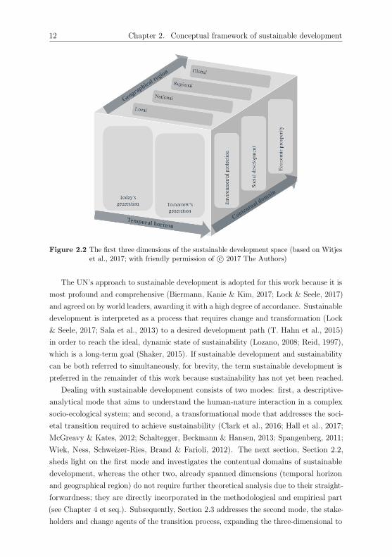
This notion constitutes the third sustainable development dimension, the geographical
region, depicted in Figure 2.2.
Despite the fact that the UN’s approach to sustainable development and sustainab-
1Some authors, e.g. Jesinghaus (2018), interpret the Agenda 21 to subdivide sustainable devel-opment into four domains: environment, society, economy, and institutions (UNCED, 1992). Asinstitutions deal with the three contentual domains, a separation at the same level is not systematic,and is thus not adopted in this work. Confirming this view, the SDG 17, “Partnerships for the goals”,does not clearly span its own, institutional domain (see Figure 2.12b).
2The term “regional” may also refer to an area smaller than the national level (e.g. Ramos &Caeiro, 2010). However, the WSSD’s (2002) classification is adopted in this work.

2.1. Definition of sustainable development and sustainability 11
Figure 2.1 The first two dimensions of the sustainable development space (based on Witjeset al., 2017; with friendly permission of c© 2017 The Authors)
ility now represents a global consensus (Costanza, Fioramonti & Kubiszewski, 2016;
Vermeulen, 2018), both terms are controversially discussed in the academic literature.
On the one hand, scholars such as T. Hahn et al. (2015); Lozano (2008); Sala et al.
(2013); Shaker (2015); and Reid (1997) are in line with the UN’s approach, interpreting
sustainable development not as a steady state but as a journey or a process of change,
adaption, and learning. Contrasting, sustainability is the ideal, dynamic state to achieve.
In this case, the pathway of sustainable development ought to be pursued in order
to obtain the long-term goal of sustainability (Dragicevic, 2018). On the other hand,
authors such as Clark et al. (2016); Holden et al. (2014); and Waas et al. (2014) use
both terms interchangeably. Further scholars such as P. James, Magee, Scerri and
Steger (2015) argue vice versa: Sustainability is the capacity to persist over time,
and therefore, it is a process to achieve the goal sustainable development (Dragicevic,
2018). An overview of different approaches to sustainable development can be found
in, e.g. Hopwood, Mellor and O’Brien (2005). Arising from the numerous existing
definitions, other works intend to capture the terminology by generating a tag cloud
of commonly-used elements in peer-review-published definitions (White, 2013). This
approach might be questionable because, for example, in highly subjective areas such
as the social domain of sustainable development (see Section 2.2.2), a larger group than
the science community should be consulted. However, for merely identifying the main
research domains, this reflective method might be legitimate (Kajikawa, Ohno, Takeda,
Matsushima & Komiyama, 2007).
12 Chapter 2. Conceptual framework of sustainable development
Figure 2.2 The first three dimensions of the sustainable development space (based on Witjeset al., 2017; with friendly permission of c© 2017 The Authors)
The UN’s approach to sustainable development is adopted for this work because it is
most profound and comprehensive (Biermann, Kanie & Kim, 2017; Lock & Seele, 2017)
and agreed on by world leaders, awarding it with a high degree of accordance. Sustainable
development is interpreted as a process that requires change and transformation (Lock
& Seele, 2017; Sala et al., 2013) to a desired development path (T. Hahn et al., 2015)
in order to reach the ideal, dynamic state of sustainability (Lozano, 2008; Reid, 1997),
which is a long-term goal (Shaker, 2015). If sustainable development and sustainability
can be both referred to simultaneously, for brevity, the term sustainable development is
preferred in the remainder of this work because sustainability has not yet been reached.
Dealing with sustainable development consists of two modes: first, a descriptive-
analytical mode that aims to understand the human-nature interaction in a complex
socio-ecological system; and second, a transformational mode that addresses the soci-
etal transition required to achieve sustainability (Clark et al., 2016; Hall et al., 2017;
McGreavy & Kates, 2012; Schaltegger, Beckmann & Hansen, 2013; Spangenberg, 2011;
Wiek, Ness, Schweizer-Ries, Brand & Farioli, 2012). The next section, Section 2.2,
sheds light on the first mode and investigates the contentual domains of sustainable
development, whereas the other two, already spanned dimensions (temporal horizon
and geographical region) do not require further theoretical analysis due to their straight-
forwardness; they are directly incorporated in the methodological and empirical part
(see Chapter 4 et seq.). Subsequently, Section 2.3 addresses the second mode, the stake-
holders and change agents of the transition process, expanding the three-dimensional to
2.2. The three contentual domains of sustainable development 13
a six-dimensional sustainable development space. The six-dimensional space is the final
conceptual framework of sustainable development, required to adequately measure and
assess sustainable development. In turn, the adequate assessment is the prerequisite for
sustainable development management and its transition (see Chapter 3; e.g. Parris &
Kates, 2003).
2.2 The three contentual domains of sustainable de-
velopment
The UNCED (1992) classified sustainable development into three contentual domains:
environmental protection, social development and economic prosperity (see Section 2.1).
The following sections, Section 2.2.1 to Section 2.2.3, review and analyse the academic
literature of these domains. Other segmentations such as the natural capital approach
by Costanza and Daly (1992), the five capital approach by Porritt (2007), or the place-
permanence-persons approach by Seghezzo (2009) are not further considered because
these attempts “explain the composition of the cake by cutting it into thinner [or
different] slices” (Hacking & Guthrie, 2008). The last section, Section 2.2.4 integrates
the three domains to a unified dimension of sustainable development.
2.2.1 Environmental protection
In the academic literature of sustainable development, the use of the terms environment
and ecology is not precise (e.g. Costanza, Fioramonti and Kubiszewski, 2016; Kates,
2015; and T. Hahn et al., 2015 vs. Hall et al., 2017; and Holden et al., 2014). Ecology
is defined as “the branch of biology that deals with the relations of organisms to one
another and to their physical surroundings” (Oxford Dictionaries, 2018a). In contrast,
the environment is defined as (1) “the surrounding or conditions in which a person,
animal, or planet lives or operates”, or as (2) “the natural world, as a whole or in
a particular geographical area, especially being affected by human activity” (Oxford
Dictionaries, 2018b). Ecology refers to the relationship between an organism and its
natural environment, whereas the environment as of definition (1) is something an
organism possesses (Mebratu, 1998). In the context of sustainable development, the term
ecology is too narrow because only the human-nature interaction would be regarded.
The first definition of the term environment is too wide since it would include, in
addition to the natural environment, the economic, political, and cultural environment
(Mebratu, 1998). These aspects are already assigned to the other two domains –
social development (see Section 2.2.2) and economic prosperity (see Section 2.2.3).
Finally, the second definition of the environment suits the sustainable development
context: The natural environment itself and the human-nature interaction are referred

14 Chapter 2. Conceptual framework of sustainable development
to simultaneously. It follows that, in this work, environmental protection is defined
as the path to environmental sustainability, a state in which the natural world is not
harmed nor degraded by human activity, such that needs of today’s generation are met
without compromising needs of tomorrow’s generation.
For highly anthropocentric reasons, the natural world is pointed at: The envir-
onmental system of the Earth is intended to remain stable because it provides life-
supporting services to humans and is thus a prerequisite for thriving societies (Griggs
et al., 2013; Kates, 2015; Steffen et al., 2015). Scientific insights deduced by the natural
science community are in the centre of the environmental domain. The main focus is
on limits or threshold values as well as interdependences of ecological and Earth system
processes (Holden et al., 2017; Patterson et al., 2017; Sala et al., 2015). Especially
the research group around Rockstrom spreads new knowledge in this field. Their
concept of planetary boundaries (Rockstrom et al., 2009a, 2009b; Steffen et al., 2015)
perfectly reflects the UN’s concept of limits (see Section 2.1). Planetary boundaries are
threshold values of life-supporting Earth system processes above which an unacceptable
global environmental change might not be possible to be avoided. This zone is the
zone of high risk. The threshold itself lies in the zone of uncertainty that features an
increasing risk. Below the boundary, the zone of safe operating space for humanity
is located. Core boundaries are boundaries “each of which has the potential on its
own to drive the Earth system into a new state should they be substantially and
persistently transgressed” (Steffen et al., 2015). Nine planetary boundaries, thereof
two core boundaries (climate change and biosphere integrity), are identified. Figure 2.3
displays the nine planetary boundaries and their current statuses of exploitation.3 The
planetary boundaries stratospheric ozone depletion, ocean acidification, and freshwater
use are currently operating in the safe zone. Climate change and land system change
are in the zone of uncertainty, while the boundaries biochemical flows and the biosphere
integrity’s subboundary genetic diversity are in the zone of high risk. For novel entities,
atmospheric aerosol loading, and the subboundary functional diversity, thresholds could
not be quantified yet.
Despite the derivation from natural science, the concept of planetary boundaries
draws on both objective and subjective matters. Measuring thresholds is objective, but
assessing and setting the level of the boundaries is highly subjective because it implies
defining the acceptable risk. Therefore, boundary setting is eventually a social decision
(Griggs et al., 2014; Leach, Raworth & Rockstrom, 2013) that requires political decision
making (see Section 2.3.3).
3Detailed descriptions of the planetary boundaries, their functioning, and role in the Earth systemare not further outlined but can be found in Rockstrom et al. (2009b).

2.2. The three contentual domains of sustainable development 15
Figure 2.3 Nine planetary boundaries and current statuses of exploitation (from Steffen et al.,2015; with permission of c© 2015, American Association for the Advancement ofScience)
2.2.2 Social development
Of the three contentual domains, the social domain of sustainable development is least
developed (Missimer, Robert & Broman, 2017a, 2017b). The concept remains open
and contested (Bostrom, 2012), different meanings circulate, and there are difficulties
in identifying purely social issues (Murphy, 2012). The literature is fragmented and
limited (Ajmal, Khan, Hussain & Helo, 2018; Dempsey, Bramley, Power & Brown,
2011), such that a further development of this domain is required (see Section 6.3).
Murphy (2012) identifies four dimensions in the social domain of sustainable de-
velopment: equity, awareness, participation, and social cohesion. Cuthill (2010) also
points out four key concepts, though, slightly different: social capital, social infrastruc-
ture, social justice and equity, and engaged governance. Overviews and more detailed
concepts of the social domain can be found in, e.g. Ajmal et al. (2018); Bostrom (2012);
Missimer et al. (2017a); Missimer et al. (2017b); and Murphy (2012). Core concepts
include, among others, quality of life, wellbeing, subjective welfare, happiness, life
satisfaction, social inclusion, dignity, affection, freedom, and safety (Harangozo, Csutora
& Kocsis, 2018; Vavik & Keitsch, 2010). These involve material as well as non-material
aspects and their achievement is highly subjective and individually determined (Mc-
Gregor & Pouw, 2017). Especially the former concepts rather refer to the developed
world, where basic needs have been successfully addressed and higher order needs are
focused (Vallance, Perkins & Dixon, 2011).4 Vallance et al. (2011) subdivide the social
domain into three categories: development sustainability, bridge sustainability, and
4Vallance et al. (2011) neither specify basic nor higher order needs. The concept of needs adoptedin this work follows shortly.
16 Chapter 2. Conceptual framework of sustainable development
maintenance sustainability. Development sustainability addresses basic needs, justice,
and equity, whereas bridge sustainability covers the changes in behaviour to achieve
environmental sustainability. Maintenance sustainability aims to preserve socio-cultural
patterns. In this work, the social domain is understood as development sustainability.
Bridge sustainability and the notion of changes in behaviour is the underlying process
of sustainable development in general, not only a means of obtaining environmental
sustainability. Furthermore, social conditions correlate with environmental protection,
but this linkage is not the focal point of the social domain. Maintenance sustainability
is disregarded as the preservation of socio-cultural patterns is not necessarily desired.
Thus, maintenance is not an overriding principle, but it is actively and explicitly gov-
erned. Further authors agree on the notion of development sustainability by Vallance
et al. (2011): In view of Ajmal et al. (2018); Holden et al. (2017); Stumpf, Baumgartner,
Becker and Sievers-Glotzbach (2015); and Stumpf, Becker and Baumgartner (2016),
social development is characterised by moral principles and philosophy on needs, equity,
and justice. Needs are in-born requirements of humans to be physically, emotionally,
and mentally healthy (Missimer et al., 2017a). Equity regards “situations in which
the claimant is equally off” (Young, 1995), whereas justice is concerned with the “fair
balance of mutual claims and obligations within a community” (Stumpf et al., 2015).
Equality also appears frequently in the context of social development and deals with
equal considerations as a claim holder or equal shares in distribution (Stumpf et al.,
2015). Because equity and equality are principles of justice (Stumpf et al., 2015; Stumpf
et al., 2016; Young, 1995), they become obsolete in working out the overarching concepts
of the social domain. The guiding principle is justice on its own, supporting the concept
of needs. Satisfaction of needs must be fairly balanced across regions (intragenerational
justice) and time (intergenerational justice) (Dower, 2004; Stumpf et al., 2015). A
definition of social development might therefore read: Social development is the path
to social sustainability, a state in which human needs of today’s generation are satisfied
in a just manner without compromising the human needs of tomorrow’s generation.
Because the core of the social domain are human needs (see Section 2.1), concepts
of human needs ought to be adduced in theorising this domain. The most well-known
concept of human needs is the hierarchy of needs by Maslow (1943).5 He points out
that humans are motivated by in-born needs that are ordered hierarchically and can
be visualised in a pyramid (see Figure 2.4). At the bottom of the pyramid are needs
that humans first seek to satisfy. After their satisfaction, needs from a higher layer
are desired to be met, until the top of the pyramid is reached. Physiological needs at
the bottom consist of homeostasis and appetite needs. Safety needs include, among
others, the need for security, protection, freedom of fear and chaos, as well as structure
and law. Belongingness and love needs are the third step on the hierarchy of needs
5Other works on human needs include, e.g. Max-Neef, Elizalde and Hopenhayn (1991), but are notfurther examined.

2.2. The three contentual domains of sustainable development 17
Figure 2.4 Maslow’s hierarchy of needs and the principle of justice (Maslow, 1943, 1987)
and refer to relations with other people to get and receive affection. Esteem needs
can be categorised into two parts: first, self-esteem such as the desire for strength,
achievement, competence, and confidence; and second, esteem of others such as desire
for reputation, fame, recognition, attention, and dignity. The last stage consists of
needs for self-actualisation, which Maslow (1987) described as the “desire to become
[...] what one idiosyncratically is”. In other words, humans desire self-fulfilment and
seek to become actualised in what they potentially are (Maslow, 1943, 1987).6 The
principle of justice is applicable to every hierarchy level: justice among physiological
needs at the bottom and justice among needs to self-actualisation at the top.
The concept of social boundaries is designed in analogy to the concept of planetary
boundaries. Social boundaries represent thresholds above which basic conditions are met
and below which critical human deprivations occur (Raworth, 2012, 2017). These bound-
aries count water, food, health, education, income and work, peace and justice, political
voice, social equity, gender equality, housing, networks, and energy (see Figure 2.5).
Water, for example, is measured as the “population without access to improved drinking
water [and sanitation]”, or food quantifies the “population undernourished” (Raworth,
2017). The setting of the threshold values and current statuses of achievement as of
Raworth (2017) are also displayed in Figure 2.5.7 Although referencing to the UN’s
approach, in particular the SDGs (see Section 2.3.3), Raworth’s social boundaries are
mainly applicable to the developing world, which is not in line with the UN suggesting
a universally applicable approach. A merger of Maslow’s hierarchy of needs, which
includes needs of the developed and the developing world, with Raworth’s concept
of social boundaries yields a valuable conceptual framework of the social domain of
sustainable development. In this connection, Maslow’s hierarchy is dissolved to a
6Maslow (1972) added self-transcendence at the top of the pyramid. However, since he did notinclude it in his work in 1987, it is also disregarded in this work.
7Worldwide data set; in the majority of cases one year of calculation between 2008 and 2015.

18 Chapter 2. Conceptual framework of sustainable development
Figure 2.5 12 social boundaries and current statuses of achievement (from Raworth, 2017;with friendly permission of c© The Author)
circle of boundaries. The dissolution is legitimate because the hierarchy might not be
significant, but needs might be independent of each other (Tay & Diener, 2011). An
illustrative example is an artist not having satisfied all material needs but being rich in
terms of self-actualisation.
2.2.3 Economic prosperity
Economic growth or profits are often incorporated in the economic domain. However,
neither economic growth nor profits are key to sustainable development, nor are they
required for a broader conception of it (Jackson, 2009; McGregor & Pouw, 2017;
Vermeulen, 2018). Even happiness does not necessarily require economic growth.
Empirical evidence suggests diminishing marginal happiness in the course of a rising
GDP per capita (p.c.) (Jackson, 2009). The misconception of economic growth or profits
being key to sustainable development can be traced back to Elkington (1997) and the
triple bottom line of people, planet, profit (Vermeulen, 2018).8 This misconception is
carried forward, and only 8% of reviewed corporate sustainable development literature
negatively invoke the term triple bottom line (Isil & Hernke, 2017). Economic prosperity
is the third contentual domain of sustainable development, and economic growth is only
needed in places where human needs are not met in order to bring people out of poverty
(Holden et al., 2014, 2017; McGregor & Pouw, 2017; WCED, 1987). In other words,
the production of resources is only required to maintain a reasonable standard of living
(Bansal, 2002). Prosperity is defined as the state of being successful in material and
financial terms (Oxford Dictionaries, 2018c, 2018d). In contrast, Jackson (2009) does
8Elkington (2018) himself requested to revise his framework of the triple bottom line. It was notdesigned to be an accounting tool that balances financial, environmental, and social aspects, but itintended to induce reflections about capitalism and its future.

2.2. The three contentual domains of sustainable development 19
Literature stream Assumption, description Example references
Degrowth eco-nomy, negativegrowth economy
The throughput of an economy can be reducedby political and social transitions while increas-ing quality of life and wellbeing.
Buch-Hansen, 2018;Harangozo et al.,2018; Kallis et al.,2018; Latouche, 2009;Magee and Devezas,2017; Schneider,Martinez-Alier andKallis, 2011
Zero growtheconomy, steadystate economy
The throughput of an economy, capital stocks,and population remain constant at a desiredmaintenance rate to stay within the planetary[and social] boundaries. Economic growth isnot required for increasing wellbeing.
H. E. Daly, 1977,1991, 1996; Har-angozo et al., 2018;Kallis et al., 2018;Kerschner, 2010
A-growth eco-nomy
Environmental effectiveness is the central pointand an a-growth economy is indifferent abouteconomic growth.
van den Bergh, 2011
Positive growtheconomy, greengrowth economy
Economic growth can be decoupled from envir-onmental usage and is based on efficiency aswell as environmental-friendly technologies.
Harangozo et al.,2018; Schneider et al.,2011; UNEP, 2011
Green economy Economic growth is not explicitly addressed,but the improvement of human wellbeing andsocial equity is focused as well as the reductionof environmental risks and ecological scarcities.
Harangozo et al.,2018; UNEP, 2010,2011
Table 2.1 Overview of (post-)growth literature streams
not define prosperity based on only material success, but prosperity further includes
social and psychological aspects. However, as these aspects are already subsumed in the
social domain (see Section 2.2.2), economic prosperity in this work follows the Oxford
Dictionaries’ definition: Economic prosperity is the path to economic sustainability, a
state in which material and financial success is achieved, such that today’s environmental
limits and social (or human) needs are met without compromising future generations’
limits and needs.
The effect of economic growth on sustainable development is ambiguous. On the
one hand, economic growth might contribute to sustainable development because
first, it might induce technological advancement required to mitigate environmental
degradation (Holden et al., 2017; Stern, 2015; van den Bergh, 2011), and second, it
might lift people out of poverty, improve social welfare, and satisfy human needs. On the
other hand, economic growth might harm sustainable development as it typically entails
environmental damages and might reduce social equality (A. B. Atkinson, 2015; Holden
et al., 2017; Piketty, 2014) and justice. Because of this ambiguity, various streams of
(post-)growth literature have emerged. These are presented in Table 2.1. Degrowth,
negative growth, zero growth, steady state, positive growth, and green growth economies

20 Chapter 2. Conceptual framework of sustainable development
are disregarded by definition since the concept of sustainable development purports
that economic growth is merely a means to an end. In contrast, an a-growth economy
and a green economy comply with this notion: Economic growth is not a driving force,
but human needs and environmental limits are centred.
Economic growth can be understood in terms of GDP, employment, consumption,
production and further measures (EC, IMF, OECD, UN & World Bank, 2009). The
most widely used economic performance measurement is the GDP, which is defined
as the “monetary market value of all final goods and services produced in a country”
(Giannetti et al., 2015; van den Bergh, 2009). GDP receives severe criticism for its
construction and its use, while its founder, Kuznets (1934a, 1934b), was well aware
of its shortcomings – or rather its pointedness. For instance, he was aware of the
fact that GDP cannot measure economic welfare because the distribution of income
and means of earning the income remain unknown. He even warned not to equalise
GDP growth and economic or social wellbeing (Costanza, Hart, Kubiszewski, Posner &
Talberth, 2018; Costanza et al., 2014; Kuznets, 1934a, 1934b). Moreover, GDP does
not differentiate between desirable and undesirable activities but positively accounts all
expenditures. For example, undesired clean-up costs of an oil spill lead to an increase in
GDP (Cobb, Halstead & Rowe, 1995; Giannetti et al., 2015; Kubiszewski et al., 2013).
GDP gives an incomplete picture by only including priced goods. Social costs such
as environmental damages are known as negative externalities and remain unpriced
with the result that GDP encourages the depletion of natural resources faster than
their renewal rate (Costanza et al., 2018; Costanza et al., 2014; Giannetti et al., 2015;
van den Bergh, 2009). Further limitations and examples can be found in, e.g. Cobb et al.
(1995); Costanza et al. (2014); Giannetti et al. (2015); Kubiszewski et al. (2013); Stiglitz,
Sen and Fitoussi (2009); and van den Bergh (2009). Even the argument that GDP
positively correlates with wellbeing indicators such as life expectancy or literacy rate is
not enough for GDP being utilised as a measure of wellbeing because a correlation does
not attest causality (van den Bergh, 2009). However, GDP is not a wrong measure, but
it is wrongly used (Giannetti et al., 2015; Stiglitz et al., 2009). Instead of attempting to
measure welfare or progress, ending up with wrong conclusions, GDP’s original purpose
should be stuck to: GDP quantifies the size of an economy in monetary terms of final
goods and services.
2.2.4 Integration of the three contentual domains
In the previous sections, Section 2.2.1 to Section 2.2.3, it has come to light that
a strict separation of the three domains is not feasible, but the three domains are
deeply interlinked (WSSD, 2002). To investigate the demanded synchronisation and
coordination of the three subsystems nature, society, and economy (Bossel, 1998;
Spangenberg, 2011), cross-disciplines such as environmental sociology, economic sociology

2.2. The three contentual domains of sustainable development 21
(Bostrom, 2012), or ecological economics (e.g. Costanza & Daly, 1992) have emerged.
The interlacing is driven by the socio-economic subsystem’s embeddedness in and
dependence on the global biophysical system (Griggs et al., 2014; Patterson et al., 2017;
Sala et al., 2015). Changes in environmental circumstances (environmental domain)
have resulted in economic gains (economic domain) but not for all people (social domain)
(Kates, 2015; Turner II et al., 1990). The principles of limits and needs are combined,
and clear cuts between the domains are challenging. Environmental pollution that
pushes people back below the social foundation (Raworth, 2012) might be interpreted as
an environmental-economic or environmental-social issue. Also, environmental pollution
that arises from higher living standards (typically leading to pollution at global level) or
environmental pollution that originates in poverty (mostly resulting in pollution at local
level (WCED, 1987)) may be classified as environmental-economic or environmental-
social problems. This example further evokes thoughts about environmental justice, and
it illustrates the ambiguous correlation of income and environmental degradation: Higher
living standards but also poverty can lead to environmental degradation. However, it
is certain that people only take up with environmental protection if their basic needs
are met (Bansal, 2002; Vallance et al., 2011). Similarly, corporations are more likely
to engage with sustainable development if they feature a strong financial performance
(Campbell, 2007). A more clear-cut example of the linkage of the environmental and
the social domains is the discussion whether an environmental tax should be a fixed or
progressive tax. Furthermore, the social and economic domains are closely intertwined
as income and prosperity brings people out of poverty, ensuring a minimum wellbeing
and typically enhancing social cohesiveness (Dragicevic, 2018). Here, ambiguities are
also present because economic prosperity at a macro level might reduce social equality, a
setback in social development (A. B. Atkinson, 2015; Holden et al., 2017; Piketty, 2014).
The relationship of the three domains are illustrated in Figure 2.6. The arrows symbolise
the direction of the relationship. Environmental protection and social development are
both focal points and mutually dependent, whereas economic prosperity only serves the
other two domains and should be adjusted according to their requirements.
On the conceptual side of integrating the three domains, the concepts of planetary and
social boundaries are combined, obeying the UN’s core concepts limits and needs. The
result is the so-called safe and just space for humanity or doughnut for the Anthropocene
(see Figure 2.7a; Raworth, 2012, 2017). The outer boundary represents the environmental
ceiling and should not be exceeded. The inner boundary expresses the social foundation
and should not be deceeded. Critical natural thresholds are located above the outer
boundary, and critical deprivations of human needs occur below the inner boundary.
As a result, the safe and just space for humanity is located below the planetary and
above the social boundaries, respectively (O’Neill, Fanning, Lamb & Steinberger, 2018;
Raworth, 2012, 2017). The current status of the safe and just operating space is

22 Chapter 2. Conceptual framework of sustainable development
Figure 2.6 Relationship of the three contentual domains
displayed in Figure 2.7b.9
Within the safe and just space, a range of possible pathways that could yield
sustainability can be mapped. The preferred trail is highly subjective because it is a
function of, among others, cultures, visions, values, costs, risks, and distribution of power
(Leach et al., 2013). The existence of a range of possible pathways makes sustainable
development a deeply political topic. The role of policy and their current goal setting
will be further discussed in Section 2.3.3. Moreover, the range of possible pathways
implies that weak sustainability can be applied. The notion of weak sustainability
originates from capital theory and assumes substitutability of the different types of
capital. Natural and manufactured capital can be reduced individually as long as the
overall level of capital passed to future generations remains constant or grows (Cabeza
Gutes, 1996; Figge & Hahn, 2004; Neumayer, 2010; Pearce & Atkinson, 1993; Pope
et al., 2017; Sala et al., 2013). This type of sustainability is often represented in a Venn
diagram (see Figure 2.8a), the most common graphical representation of sustainability
(Dragicevic, 2018; Lozano, 2008; Mebratu, 1998). On the contrary, strong sustainability
assumes that the different types of capital are complements and need to be preserved
for future generations (Costanza & Daly, 1992; H. E. Daly, 1990; Dragicevic, 2018;
Figge & Hahn, 2004; Neumayer, 2010; Sala et al., 2013). Therefore, the capital with
the shortest supply is a limiting factor (H. E. Daly, 1990; Dragicevic, 2018). The
graphical representation of strong sustainability is often a concentric diagram (see
Figure 2.8b; Dragicevic, 2018; Griggs et al., 2013; Lozano, 2008; Mebratu, 1998), with
the environmental domain on the outside and the economic domain on the inside because
the socio-economic subsystem is embedded in the global biophysical system (see above;
Patterson et al., 2017; Sala et al., 2015).10 Strong sustainability is in line with most
9Denotations and statuses of the boundaries slightly differ from Steffen et al. (2015; see Figure 2.3).10Lozano (2008) suggests further graphical representations grounded in a critical review of the
existing visualisations. Major criticism includes compartmentalisation of the linked domains and themissing representation of dynamics.

2.2. The three contentual domains of sustainable development 23
(a) The concept of the safe and just operatingspace for humanity
(b) Current statuses of the nine planetary and12 social boundaries
Figure 2.7 The safe and just operating space for humanity (based on/from Leach et al.,2013; Raworth, 2012, 2017; with friendly permissions of c© ISSC, UNESCO 2013;c© Oxfam International February 2012; c© 2017 The Author)
ecological economists (e.g. Costanza & Daly, 1992; H. E. Daly, 2005; Holden et al.,
2014; Isil & Hernke, 2017). The reasons behind are twofold. First, the anthropocentric,
natural science perspective recognises that human outcomes depend on the functioning
of the Earth system (O’Neill et al., 2018) and acknowledges that the limiting factor has
become exactly this system (Costanza & Daly, 1992; H. E. Daly, 2005). Second, from
an economic perspective, strong sustainability is required as natural and manufactured
capital are often complements by their nature (Costanza & Daly, 1992). Synthesising
Leach et al.’s (2013) and the ecological economists’ viewpoints, weak sustainability,
which is allowed within the safe and just operating space for humanity, should be
accompanied by minimised substitutability to respond to both factor limitations and
complementarity. However, outside the safe and just space, strong sustainability must
be applied because factors of the environmental or the social domain are exhausted and
thus become limiting factors. The environmental and the social boundaries must be
known to determine whether weak or strong sustainability should be in use.
After dealing with the descriptive-analytical mode of sustainable development by
analysing the three contentual domains and their linkages, the next section, Section 2.3,
examines stakeholders and change agents of sustainable development. These are
prerequisites for the second, transformational mode of sustainable development that
aims to put the normative concept of sustainable development into practice (see
Section 2.1; Wiek et al., 2012).

24 Chapter 2. Conceptual framework of sustainable development
(a) Venn diagram of the contentual domains,visualising weak sustainability
(b) Concentric diagram of the contentual do-mains, visualising strong sustainability
Figure 2.8 Venn and concentric diagrams of weak and strong sustainability (based onDragicevic, 2018; Griggs et al., 2013; Lozano, 2008; Mebratu, 1998; with friendlypermissions of c© 2018 John Wiley & Sons, Ltd and ERP Environment; c© 2013Macmillan Publishers Limited. All rights reserved; c© 2008 Elsevier Ltd. Allrights reserved; c© 1998 Elsevier Science Inc. All rights reserved)
2.3 Stakeholders and change agents of sustainable
development
At the start of the UN’s debate on sustainable development in the 1970s, the UNCHE
(1972) recognised that citizens, communities, enterprises, and institutions at any level
should share equitable efforts in the sustainability transition. Groups or individuals
that can affect or be affected by actions are stakeholders (Freeman, 1984, 2010; Horisch,
Freeman & Schaltegger, 2014). Change agents are defined as “internal or external
actors that play a significant role in initiating, managing, or implementing change”
(Caldwell, 2003; van Poeck et al., 2017). Because sustainable development requires
change and transformation (see Section 2.1; e.g. Lock & Seele, 2017), it is desired that
all stakeholders become change agents who devote actions, behaviour, decision making,
and solutions (Hall et al., 2017) towards sustainable development. Thus, the change
agent group builds the fourth dimension of the sustainable development framework and
can be arranged into four clusters: business, policy, society (Hajer et al., 2015), and
science (Lock & Seele, 2017).11 Each group acts on every sustainable development
dimension. To facilitate the visualisation of the sustainable development space, the
11Lock and Seele (2017) divide change agents into several categories: companies, governments,Intergovernmental Organisations (IGOs), private citizens, non-governmental organisations, charitableorganisations or non-profit organisations, grassroot organisations, media, future generations (though,being passive stakeholders), and academia. For this work, this granularity is not required but thegeneral structure is adopted.
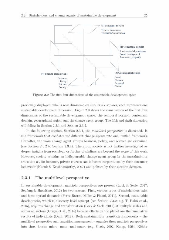
2.3. Stakeholders and change agents of sustainable development 25
Figure 2.9 The first four dimensions of the sustainable development space
previously displayed cube is now disassembled into its six squares; each represents one
sustainable development dimension. Figure 2.9 shows the visualisation of the first four
dimensions of the sustainable development space: the temporal horizon, contentual
domain, geographical region, and the change agent group. The fifth and sixth dimension
will follow in Section 2.3.1 and Section 2.3.2.
In the following section, Section 2.3.1, the multilevel perspective is discussed. It
is a framework that conflates the different change agents into one, unified framework.
Hereafter, the main change agent groups business, policy, and science are examined
(see Section 2.3.2 to Section 2.3.4). The group society is not further investigated as
deeper insights from sociology or further disciplines are beyond the scope of this work.
However, society remains an indispensable change agent group in the sustainability
transition as, for instance, private citizens can influence corporations by their consumer
behaviour (Kucuk & Krishnamurthy, 2007) and politics by their election decision.
2.3.1 The multilevel perspective
In sustainable development, multiple perspectives are present (Lock & Seele, 2017;
Seyfang & Haxeltine, 2012) for two reasons. First, various types of stakeholders exist
and have myriad demands (Perez-Batres, Miller & Pisani, 2011). Second, sustainable
development, which is a society level concept (see Section 2.3.2; e.g. T. Hahn et al.,
2015), requires change and transformation (Lock & Seele, 2017) at multiple scales and
across all sectors (Griggs et al., 2014) because effects on the planet are the cumulative
results of individuals (Dahl, 2012). Both sustainability transition frameworks – the
multilevel perspective and transition management – organise these multiple perspectives
into three levels: micro, meso, and macro (e.g. Geels, 2002; Kemp, 1994; Kohler

26 Chapter 2. Conceptual framework of sustainable development
et al., 2019; Loorbach, 2010; Markard, Raven & Truffer, 2012; Rip & Kemp, 1998;
Rotmans et al., 2001; Smith, Voß & Grin, 2010). By doing so, the big picture and
the broader problem framing can be captured (Smith et al., 2010), which is in turn
necessary for a successful transition to sustainability. Only if multiple actors cooperate,
their actions can intensify each other, leading to a successful transition (Loorbach,
2007). On the one hand, the multilevel perspective regards technological change for
sustainable development and organises the analysis into niches (micro), regimes (meso),
and landscapes (macro) (e.g. Geels, 2002; Kemp, 1994; Loorbach, 2007; Rip & Kemp,
1998; Smith et al., 2010). Niche is the level of innovation inside which novelties are
created, tested, and diffused. A regime is the “dominant culture, structure and practice
embodied by physical and immaterial infrastructures”, whereas a landscape is defined
as the overall societal setting (e.g. social values, political cultures, or economic trends),
in which a process of technological change occurs (Loorbach, 2007).12 Given its focus on
technological change, this framework is not further regarded in this work. On the other
hand, the transition management framework by Rotmans et al. (2001) is of relevance
for this work because it is a decision-oriented framework that sorts the aggregational
size of stakeholders and change agents of sustainable development into micro, meso,
and macro. A micro object comprises individuals and individual actors, a meso object
is composed of networks, communities, or organisations, whereas a macro object is a
conglomerate of institutions or organisations. Because this framework also addresses
micro, meso, and macro levels, it is also referred to as the multilevel perspective. Every
stakeholder can be divided to the three aggregational sizes. For example, business
may be an individual economic agent (micro), a corporation (meso), or a branch or an
overall economy (macro); policy may be a single politician (micro), a single national
government (meso), or an IGO (macro); and so on ad nauseam. Figure 2.10 illustrates
this novel dimension within the sustainable development space, which is disregarded
in existing sustainable development frameworks (see Chapter 2; e.g. Chofreh & Goni,
2017). This perspective gap is closed by the present framework. The sixth and last
dimension follows in the next section, Section 2.3.2, which deals with the change agent
group business.
2.3.2 Corporate sustainability
Without dedication and leadership by corporations to sustainable development, sus-
tainable development will not be reached (Sachs, 2012). Sustainable production and
consumption are the major challenges of sustainable development (Sala et al., 2013;
Weitz et al., 2018), and corporations represent the productive sources of the economy,
producing and consuming resources (Bansal, 2002; T. Hahn & Figge, 2011).
12Further definitions of landscapes, regimes, and niches exist and can be found in, e.g. Geels (2002);and Rip and Kemp (1998).
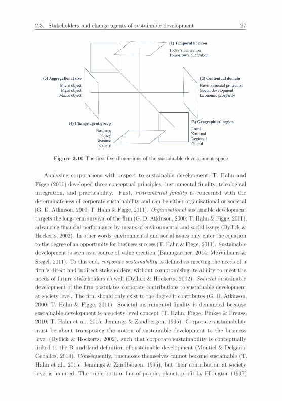
2.3. Stakeholders and change agents of sustainable development 27
Figure 2.10 The first five dimensions of the sustainable development space
Analysing corporations with respect to sustainable development, T. Hahn and
Figge (2011) developed three conceptual principles: instrumental finality, teleological
integration, and practicability. First, instrumental finality is concerned with the
determinateness of corporate sustainability and can be either organisational or societal
(G. D. Atkinson, 2000; T. Hahn & Figge, 2011). Organisational sustainable development
targets the long-term survival of the firm (G. D. Atkinson, 2000; T. Hahn & Figge, 2011),
advancing financial performance by means of environmental and social issues (Dyllick &
Hockerts, 2002). In other words, environmental and social issues only enter the equation
to the degree of an opportunity for business success (T. Hahn & Figge, 2011). Sustainable
development is seen as a source of value creation (Baumgartner, 2014; McWilliams &
Siegel, 2011). To this end, corporate sustainability is defined as meeting the needs of a
firm’s direct and indirect stakeholders, without compromising its ability to meet the
needs of future stakeholders as well (Dyllick & Hockerts, 2002). Societal sustainable
development of the firm postulates corporate contributions to sustainable development
at society level. The firm should only exist to the degree it contributes (G. D. Atkinson,
2000; T. Hahn & Figge, 2011). Societal instrumental finality is demanded because
sustainable development is a society level concept (T. Hahn, Figge, Pinkse & Preuss,
2010; T. Hahn et al., 2015; Jennings & Zandbergen, 1995). Corporate sustainability
must be about transposing the notion of sustainable development to the business
level (Dyllick & Hockerts, 2002), such that corporate sustainability is conceptually
linked to the Brundtland definition of sustainable development (Montiel & Delgado-
Ceballos, 2014). Consequently, businesses themselves cannot become sustainable (T.
Hahn et al., 2015; Jennings & Zandbergen, 1995), but their contribution at society
level is haunted. The triple bottom line of people, planet, profit by Elkington (1997)
28 Chapter 2. Conceptual framework of sustainable development
is not only a misconception in the society level concept of sustainable development
but also in corporate sustainability. In the society level concept, economic prosperity
and not economic growth is key to sustainable development (see Section 2.2.3; e.g.
Vermeulen, 2018); for corporate sustainability, also economic prosperity and not profit is
key as societal instrumental finality is required (see above). Furthermore, the defensive
approach of corporate social responsibility is not enough because it only addresses
corporations’ responsibility to society and regards the moral obligation of managers
(Bansal & Song, 2017). Only negative impacts of businesses on society are eliminated
(Baumgartner, 2014; Carpenter & White, 2004), but contributions to sustainable
development must be tackled by a scientific system perspective (Bansal & Song, 2017).
This perspective is pursued by corporate sustainability and societal instrumental finality.
Second, teleological integration deals with the integration of environmental, social,
and economic aspects (T. Hahn & Figge, 2011). This integration is seen as a major
challenge in post-modern society and thus in corporate sustainability (Gladwin, Kennelly
& Krause, 1995; T. Hahn & Figge, 2011; Taylor, 1989) as the interlinkages include
tensions (T. Hahn et al., 2015). Tensions may arise along each sustainable development
dimension visualised in Figure 2.10, forthcoming in Figure 2.11.13 Four management
approaches are identified that cope with tensions. The win-win perspective regards
situations in which the three domains are in harmony, such that economic, social, and
environmental objectives can be reached simultaneously (T. Hahn et al., 2010). The
business case for sustainable development is realised (Dyllick & Hockerts, 2002; T. Hahn
et al., 2010) by avoiding tensions through alignment of the three domains. This typically
implies an economic bias, which is referred to as bounded instrumentality (T. Hahn &
Figge, 2011; T. Hahn et al., 2010; van der Byl & Slawinski, 2015). The triple bottom
line leads to bounded instrumentality. By limiting itself to profit maximisation, this
perspective is likely to dismiss potential positive corporate contributions to sustainable
development (T. Hahn et al., 2010). The trade-off perspective recognises that there
are situations in which the three domains cannot be obtained simultaneously. Owing
to the multidimensionality of sustainable development, these situations are rather the
rule than the exception,14 and thus, corporate sustainability is required to conceptually
be able to deal with trade-offs (T. Hahn & Figge, 2011; T. Hahn et al., 2010). In this
management perspective, tensions are avoided by choosing one sustainable development
element over the other. Typically, profits are sought to be maximised (van der Byl &
Slawinski, 2015). Thinking “beyond the business case” is required (Dyllick & Hockerts,
13According to T. Hahn et al. (2015), tensions may only arise along three dimensions: levels, processof change, and context. Levels refer to the aggregational size and can be individuals, organisations, orsystems. This view is in line with the multilevel perspective by Rotmans et al. (2001) (see Section 2.3.1).Process of change regards the three contentual domains, and context refers to the temporal and spatialcontext (i.e. intergenerational and intragenerational aspects, respectively).
14Opposing, Pradhan et al. (2017) conclude in their empirical study that there are typically moresynergies than trade-offs. Nonetheless, conceptual ability to deal with trade-offs remains essentialbecause they have to be managed regardless of their relative frequency.

2.3. Stakeholders and change agents of sustainable development 29
Figure 2.11 The six-dimensional sustainable development space and the three conceptualprinciples of its management
2002; T. Hahn & Figge, 2011; T. Hahn et al., 2010, 2018; T. Hahn et al., 2015), and
businesses should not have any a priori economic superiority (T. Hahn & Figge, 2011)
but simultaneously address the three, interconnected sustainable development domains
(T. Hahn et al., 2015). The integrative perspective requests managers to pursue different
sustainable development aspects at once even if they are oppositional (T. Hahn et al.,
2015). The focus is shifted from economic to environmental and social issues (van der
Byl & Slawinski, 2015), and solutions for the entire system of interrelated elements are
looked for (Gao & Bansal, 2013). Last, the paradox perspective explicitly acknowledges
tensions (T. Hahn et al., 2018) by coexistence of oppositional elements (Clegg, Vieira da
Cunha & Pina e Cunha, 2002; T. Hahn et al., 2015; Lewis, 2000). These situations are
managed by first accepting the contradictions and second exploring them (van der Byl
& Slawinski, 2015), such that managers are able to achieve competing objectives (T.
Hahn et al., 2018). T. Hahn et al. (2018); T. Hahn et al. (2015); and van der Byl and
Slawinski (2015) agree that in terms of teleological integration, the paradox perspective
must be implemented. Notwithstanding, Landrum and Ohsowski (2018) find that the
dominating mindset is the business case for sustainable development, which neither
acknowledges the paradox theory nor tensions in general.
Third, practicability refers to the need of effectively informing and guiding decision
makers (Boron & Murray, 2004; T. Hahn & Figge, 2011). These three conceptual
principles do not only apply to their original field of corporate sustainability but can
be transferred to the management of sustainable development in general. Therefore,
they enter the conceptual framework of sustainable development (see Figure 2.11).
The three conceptual principles – societal instrumental finality, paradox teleological
integration, and practicability – are urged to be embedded into all decisional tiers

30 Chapter 2. Conceptual framework of sustainable development
(Engert, Rauter & Baumgartner, 2016; Galbreath, 2009; R. Hahn, 2013), opening the
sixth and last dimension of the sustainable development space. The decisional tier can
be divided into three levels: normative, strategic, and operational (Baumgartner, 2014;
Ulrich, 2001). The normative tier deals with the management philosophy and basic
beliefs as well as values of the corporation that influence behaviours and decisions of
management and employees (Baumgartner, 2014; Ulrich, 2001). The strategic tier is
responsible for the effectiveness of the sustainability strategy. The process of planning,
implementing, and evaluating effects is dealt with in order to achieve the long-term goals
(Baumgartner, 2014; David, 2009). The operational tier is concerned with efficiency
and implements normative and strategic goals (Baumgartner, 2014; Ulrich, 2001).
This model is known as the St. Gallen management model (Ulrich, 2001). Similar to
the conceptual principles, the decisional tiers are not only of relevance for corporate
sustainability but for sustainable development management in general, entering the
conceptual framework. The final version of the framework, with its six dimensions and
three conceptual principles, is pictured in Figure 2.11. Despite the need to address
all three decisional tiers, many corporations only integrate corporate sustainability
at the operational tier (Engert et al., 2016; Galbreath, 2009; R. Hahn, 2013). This
operational-to-normative gap is seen as the major reason in the lack of progress towards
(corporate) contributions to sustainable development (Baumgartner & Rauter, 2017;
Tseng et al., 2018) and is hence taken into consideration in the selection process of the
sustainable development measurement method (see Section 3.1 to Section 3.2).
Generally, corporations need an incentive to engage in corporate contributions
to sustainable development (T. Hahn & Figge, 2011; Husted & de Jesus Salazar,
2006). Incentives and drivers can be of internal or external nature (Lozano, 2015), and
several theories exist to explain engagements in corporate sustainability. An overview
on literature streams, their main assumptions, and example references from theory-
building, summarising, or empirical studies are given in Table 2.2. The last column of
Table 2.2 evaluates the fulfilment of the respective theory with the conceptual principles
of societal instrumental finality and paradox teleological integration (see Figure 2.11).
Practicability is not meaningful to be evaluated in this context but will be taken up on
in Chapter 3. The natural resource-based view focuses on competitive advantage and
maximisation of the firm, such that bounded instrumentality is present. The win-win
or the trade-off perspective might be the managing view. Institutional, legitimacy,
and stakeholder theories are driven by stakeholders and therefore may fit the criteria
of instrumental finality and teleological integration if stakeholders desire or enforce
these. Stewardship theory and sustaincentrism are the only theories that conceptually
include societal instrumental finality and paradox teleological integration at any time.
Consequently, corporations are encouraged to take actions to employ stewards and
implement sustaincentrism in their organisation. Further studies on drivers of corporate
sustainability include Engert et al. (2016); and Lozano (2015). Eccles, Ioannou and

2.3. Stakeholders and change agents of sustainable development 31
Literature
stream
Assumption
Example
references
Societal
instrumentalfinal-
ity
and
paradox
teleolo-
gicalintegration
Natural
resource-
basedview,agency
theory
Corporationsdep
endon
naturalan
dman
u-
facturedresources
andrega
rdtheirscarcity
togain
competitiveadvantage.
Managers
are
rationalagents
andmaxim
iseprofits.
T.H
ahnan
dFigge,20
11;Hart,19
95;Hartan
dDow
ell,
2011;JensenandMeckling,1976;McW
illiamsand
Siegel,2011;Montiel
andDelgado-C
eballos,
2014
No
Stakeholder
theory
Corporationskeep
the
interest
oftheir
stakeholdersin
mindin
order
toachieve
asuperiorperform
ance.
Freem
an,1984,2010;R.HahnandKuhnen,2013;
Lap
lume,Son
par
andLitz,20
08;Mon
tielan
dDelga
do-
Ceballos,
2014
;Perez-B
atreset
al.,20
11;Shevchenko,
LevesqueandPagell,2016
Only
ifstak
eholdersdesire
Legitim
acy
theory
Corporationsrequirealicence
tooperate,
grantedbytheirstakeholders.
BansalandClelland,2004;Baumgartner,2014;Dee-
gan,2002;DiM
aggio
andPow
ell,1983;Dow
lingand
Pfeffer,1975;R.Hahn
and
Kuhnen,2013;Perez-
Batres
etal.,2011;Schaltegger
andHorisch,2017;
Suchman,1995
Only
ifstak
eholdersdesire
Institution
altheory
Institution
alculture
ofthecorporationen-
ablesan
dconstrainsbeh
aviour.
Campbell,2007;DiM
aggio
andPow
ell,1983;Egels-
Zanden
and
Wahlqvist,
2007;
Galbreath,
2010;
LinnenlueckeandGriffiths,
2010;J.W
.Meyer
and
Row
an,1977;Montiel
andDelgado-C
eballos,
2014
Only
ifregulations
or
stakeholdersenforceand
institutionalise
Stewardship
theory
Managersreceive
ahigher
utility
from
pro-organisational,collectivisticthanself-
servingbeh
aviouran
dactively
shap
epath-
waysofsocialandenvironmentalchange.
Davis,Schoorman
andDon
aldson,19
97;Folke,Biggs,
Norstrom,Reyersan
dRockstrom,20
16;Godos-D
ıez,
Fernan
dez-G
agoan
dMartınez-C
ampillo,20
11;Tseng
etal.,2018
Yes
Sustaincentrism
Man
agersaregu
ided
byan
environ
mental
andmoralcompass.
Gladwin
etal.,1995;Montiel
andDelgado-C
eballos,
2014;Valente,2012
Yes
Table
2.2
Overview
ofliterature
streamsofcorporate
sustainabilitydrivers

32 Chapter 2. Conceptual framework of sustainable development
Serafeim (2014) investigate vice versa and tackle the impact of corporate sustainability
on organisational processes and performances.
2.3.3 Political goal setting: The United Nations’s (UN) Sus-
tainable Development Goals (SDGs)
Policy making and the involvement of governments are inherent in sustainable develop-
ment (Meadowcroft, 1997, 2011). The subjective nature of sustainable development
means going beyond efficiency and deciding upon one of the multiple pathways (see
Section 2.2.4; Leach et al., 2013), requiring negotiations in a democratic system (Mc-
Gregor & Pouw, 2017). Moreover, governments exercise control by launching laws or
regulations and by providing public goods such as infrastructure (Clarkson, 1995; Hood
& Margetts, 2007; Lock & Seele, 2017). IGOs frame political interactions (Meadowcroft,
2011), and in this vein, the UN has released the most elaborated concept of sustainable
development (see Section 2.1; Lock & Seele, 2017). Further international organisations
such as the Organisation for Economic Co-operation and Development (OECD) and
International Labour Organization (ILO) spread advices on political landscapes and
legal frameworks for sustainable development in documents such as ILO (2013); and
OECD (2016).15 However, as in previous sections, this work continues to concentrate
on the UN’s approach to sustainable development. Section 2.1 has dealt with the
normative concept of the UN’s approach, whereas this section regards the strategic
level and the release of development goals.
The first development goals were the Millennium Development Goals (MDGs). The
MDGs are an integrated framework adopted by 189 countries around the world in
the 2000s, aiming at social development and improved living standards of the world’s
poor (Glaser, 2012; Griggs et al., 2014; Sachs, 2012; UNGA, 2000). With the MDGs,
measurable and timebound objectives were set, promoting global awareness, political
accountability, social feedback, and public pressure for sustainable development (Sachs,
2012). In 2015, the MDGs were replaced by the SDGs. The SDGs do not only embrace
developing countries but are universally applicable to all countries and geographical
regions (Glaser, 2012; Sachs, 2012). Given the third dimension of the sustainable
development space (see Figure 2.11), an essential improvement is realised. The SDGs
promote social development and economic prosperity in harmony with nature for all
nations and are globally accepted as the content and meaning of sustainable development
(Dahl, 2018; UNCSD, 2012; UNGA, 2015). There are 17 SDGs with 169 targets and 232
indicators in total. The goals and targets are agreed on by international negotiation,
whereas the indicators are worked out and annually refined by an expert group (UN,
2018, 2019a; UNGA, 2015). With the numerous, quantitative indicators, progress can
be monitored, policy may be informed, and accountability of all stakeholders can be
15The ILO focuses topics of labour and thus only regards the social or economic domain.

2.3. Stakeholders and change agents of sustainable development 33
ensured (UN, 2019a). The SDGs are, similar to the MDGs, voluntary, time-bounded
targets (Glaser, 2012) and can be summarised to poverty elimination, sustainable
lifestyles for all, and a stable resilient planetary life-supporting system (Griggs et al.,
2014). In detail, the 17 SDGs read (UN, 2018):
• SDG 1: End poverty in all its forms everywhere.
• SDG 2: End hunger, achieve food security and improved nutrition, and promotesustainable agriculture.
• SDG 3: Ensure healthy lives and promote wellbeing for all at all ages.
• SDG 4: Ensure inclusive and equitable quality education and promote lifelonglearning opportunities for all.
• SDG 5: Achieve gender equality and empower all women and girls.
• SDG 6: Ensure availability and sustainable management of water and sanitationfor all.
• SDG 7: Ensure access to affordable, reliable, sustainable, and modern energyfor all.
• SDG 8: Promote sustained, inclusive, and sustainable economic growth; fulland productive employment; and decent work for all.
• SDG 9: Build resilient infrastructure, promote inclusive and sustainable indus-trialisation, and foster innovation.
• SDG 10: Reduce inequality within and among countries.
• SDG 11: Make cities and human settlements inclusive, safe, resilient, and sus-tainable.
• SDG 12: Ensure sustainable consumption and production patterns.
• SDG 13: Take urgent action to combat climate change and its impacts.
• SDG 14: Conserve and sustainably use the oceans, seas, and marine resourcesfor sustainable development.
• SDG 15: Protect, restore, and promote sustainable use of terrestrial ecosystems;sustainably manage forests; combat desertification; halt and reverseland degradation; and halt biodiversity loss.
• SDG 16: Promote peaceful and inclusive societies for sustainable development;provide access to justice for all; and build effective, accountable, andinclusive institutions at all levels.
• SDG 17: Strengthen the means of implementation and revitalise the globalpartnership for sustainable development.
Figure 2.12a displays the 17 SDGs and Figure 2.12b shows their allocation to the
three contentual domains. Four goals are assigned to the environmental domain, eight
goals belong to the social domain, another four goals make up the economic domain and
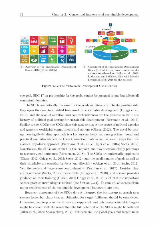
34 Chapter 2. Conceptual framework of sustainable development
(a) Overview of the Sustainable DevelopmentGoals (SDGs) (UN, 2019b)
(b) Assignment of the Sustainable DevelopmentGoals (SDGs) to the three contentual do-mains (from/based on Folke et al., 2016;Rockstrom and Sukhdev, 2014; with friendlypermission of c© 2016 by the authors)
Figure 2.12 The Sustainable Development Goals (SDGs)
one goal, SDG 17 on partnership for the goals, cannot be assigned to any but affects all
contentual domains.
The SDGs are critically discussed in the academic literature. On the positive side,
they open the door to a unified framework of sustainable development (Griggs et al.,
2014), and the level of ambition and comprehensiveness are the greatest so far in the
history of political goal setting for sustainable development (Biermann et al., 2017).
Similar to the MDGs, the SDGs place this goal setting at the centre of political agendas
and generate worldwide commitments and actions (Glaser, 2012). The novel bottom-
up, non-legally-binding approach is a key success factor as, among others, moral and
practical commitments feature lower transaction costs as well as fewer delays than the
classical top-down approach (Biermann et al., 2017; Hajer et al., 2015; Sachs, 2012).
Nonetheless, the SDGs are explicit in the endpoint and may therefore clarify pathways
to necessary end outcomes (Vermeulen, 2018). The SDGs are universally applicable
(Glaser, 2012; Griggs et al., 2013; Sachs, 2012), and the small number of goals as well as
their simplicity are essential for focus and effectivity (Griggs et al., 2014; Sachs, 2012).
Yet, the goals and targets are comprehensive (Pradhan et al., 2017). Besides, they
are practicable (Sachs, 2012), measurable (Griggs et al., 2013), and science provides
guidance on their framing (Glaser, 2012; Griggs et al., 2014), such that the important
science-practice interlinkage is realised (see Section 2.3.4). To sum up, advocates claim
major requirements of the sustainable development framework are met.
However, opponents of the SDGs do not interpret the bottom-up approach as a
success factor but claim that an obligation for target fulfilment should be established.
Otherwise, counterproductive drivers are supported, and only easily achievable targets
might be chosen with the result that the full potential of the SDGs might be forfeited
(Allen et al., 2019; Spangenberg, 2017). Furthermore, the global goals and targets must
2.3. Stakeholders and change agents of sustainable development 35
be translated into corresponding efforts at the national level (Dahl, 2018). In addition,
the SDGs are said to be vague, weak, or meaningless (Holden et al., 2017; Stokstad,
2015). 54% of the targets require further work and need to be strengthened by, for
instance, determining endpoints and time frames for an accurate measurement. 17% of
the targets are non-essential and can be disregarded (ICSU & ISSC, 2015; Stokstad,
2015). Spaiser et al. (2017) reinforce these qualitative assertions by empirical evidence
derived by several multivariate techniques. They conclude that the economic domain is
valid, the social domain is well represented, but the environmental domain is poorly
defined and incoherent. Scholars generally agree that further research is demanded in the
environmental domain, among others, the planetary boundaries must be linked to the
SDGs and broken down to national or corporate level (see Section 2.2.1 and Section 6.3;
e.g. O’Neill et al., 2018; Whiteman et al., 2013). Further criticism involves that there
are repetitions and that the environmental goals 12 to 15 are not quantifiable (Holden
et al., 2017).16 The author of this work does not agree on this criticism as the UN (2018)
lists numerous solid, quantitative indicators. Nonetheless, the author agrees on Holden
et al.’s (2017) criticism that the SDGs rest on wrong premises by balancing the three
dimensions. The UN (2018) includes economic growth as a sustainable development
indicator but does not specify a threshold above which economic growth is not required
anymore. Further criticism includes having too many goals results in not having a
goal at all. Therefore, only relevant indicators should be chosen (see Section 3.1; Hak,
Janouskova & Moldan, 2016; Holden et al., 2017; Janouskova, Hak & Moldan, 2018;
Reyers, Stafford-Smith, Erb, Scholes & Selomane, 2017). Reyers et al. (2017) offer an
approach to monitor the SDGs with only essential variables. Moreover, prioritisation
of the SDGs is a prerequisite for effectiveness of actions. The SDGs are individually
straight forward but the system as a whole, its dynamics, synergies, and trade-offs
have to be understood (Allen et al., 2019; Nilsson et al., 2016; Pradhan et al., 2017;
Sachs, 2012; Spaiser et al., 2017; Weitz et al., 2018). This knowledge gap must be
solved for maximising progress on the SDGs (Costanza, Fioramonti & Kubiszewski,
2016; ICSU & ISSC, 2015; Spaiser et al., 2017; Weitz et al., 2018), critically determining
the selection process of the sustainable development assessment method (see Section 3.1
to Section 3.2). If decision makers ignore the interlinkages and overlaps, important
contributions to sustainable development may be missed. However, decision makers
require science-based assistance for complexity reduction and prioritisation. First works
on SDG prioritisation include, for instance, Allen et al. (2019); Pradhan et al. (2017);
and Weitz et al. (2018). New insights on the system dynamics, synergies, and trade-offs
will be contributed by the empirical part of this work (see Chapter 5).
To sum up, the SDGs entail both risks and opportunities: The SDGs bear the risk of
16Folke et al. (2016); and Rockstrom and Sukhdev (2014) assign SDG 12 on responsible consumptionand production to the economic domain. The author of this work rather agrees with Holden et al.(2017) and the SDG 12 being an environmental goal (see Section 5.3.1).

36 Chapter 2. Conceptual framework of sustainable development
creating a huge bureaucratic burden with failure of practical results, and they have the
potential to transform the globe towards sustainable development. To reduce the risk
of failure, the knowledge gap must be closed. This is a task for the science community
(including this work), which is characterised in the next section, Section 2.3.4.
2.3.4 Sustainability science
Last, the science community is fundamental in the process of sustainable development
because it crafts knowledge, facilitates the transition with the new knowledge, passes
the knowledge on to young people in institutions of higher education, and publishes
the information for the public (Bachmann, 2016; Barth, 2016; Clark, 2007; Clark et al.,
2016; Folke et al., 2016; Lock & Seele, 2017). The discipline sustainability science was
initiated by Kates et al. (2001), decades after the start of the intergovernmental debate
headed by the UN (see Section 2.1 and Section 2.3.3). Kates (2015); and Kates et al.
(2001) raised seven core questions to be answered by the discipline, drawing on both
the descriptive-analytical and the transformational mode (see Section 2.1; Wiek et al.,
2012). The dual mission of sustainability science (Hall et al., 2017; McGreavy & Kates,
2012) shapes this discipline, always seeking solutions to real world problems and being
teleologically directed towards sustainable development (Spangenberg, 2011). Most
importantly is the connection of science (knowledge) and practice (societal action and
informed decision making) between which sustainability science creates a dynamic bridge
(Clark, 2007; Kates, 2015; Sala et al., 2015; Turner II et al., 2003). To manage both
the descriptive-analytical and the transformational mode, sustainability science needs
to be transdisciplinary (Jahn, Bergmann & Keil, 2012; Lang et al., 2012; Schaltegger
et al., 2013; Spangenberg, 2011). Transdisciplinary research is not only characterised
by science-practice collaborations that focus on societally relevant problems and seek
for real-world solutions, but also by methodological pluralism and collaborations of
various disciplines (Lang et al., 2012; Schaltegger et al., 2013; Spangenberg, 2011).17
In sustainability science, pluralism is required to handle the complexity arising from
the multidimensionality of the framework. A conceptual agenda for transdisciplinary
research can be found in Jahn et al. (2012); and Lang et al. (2012) and is reproduced in
Figure 2.13. Societal and scientific practice work hand in glove. During the first phase
(Phase A), a societal problem is identified and triggers the scientific research question.
Herefrom, the joint problem is framed, and collaborative teams from academia and
practice are built, such that mutual learning among researchers and practitioners is
enabled. In Phase B, solution-oriented and transferable knowledge is generated and
disclosed. Subsequently, this knowledge is reintegrated and applied, leading to useful
and relevant results for social and scientific practice in Phase C. This in turn loops
17A detailed differentiation of disciplinary, multidisciplinary, interdisciplinary, and transdisciplinaryresearch can be found in Schaltegger et al. (2013).

2.3. Stakeholders and change agents of sustainable development 37
Figure 2.13 Conceptual agenda of a transdisciplinary research processes (based on Jahnet al., 2012; Lang et al., 2012; with friendly permissions of c© 2012 Elsevier B.V.All rights reserved; c© Springer 2012)
back into Phase B and Phase A.
Taking into account the research reviewed for this work, the discipline sustainability
science has accomplished Phase A to the point of being on hold for further feedback
loops. Societal and scientific problems are framed, which, for example, resulted in the
SDGs (see Section 2.3.3). The development of a sustainable development indicator set
demands scientific knowledge production as well as political norm creation (Rametsteiner,
Pulzl, Alkan-Olsson & Frederiksen, 2011). The SDGs successfully draw this line from
science to practice first by the process itself (see Section 2.3.3) and second by providing
results of the goals, targets, and indicators for political decision making as well as
scientific analysis. Actor specific and scientific disclosure (Phase B) has been performed.
Examples include corporations that disclose sustainability reports in accordance with
the standard of the GRI (see Section 3.3.1; GRI, 2016) and the growing number of
academic publications (Kates, 2015). Phase C has been entered but it is not finalised
yet, such that sustainable development remains a vision of future (White, 2013). Useful
and relevant results for society and science have been generated but are not completed.
On the scientific side, not all planetary boundaries have been quantified, the concept of
social boundaries demands further refinement, and the corresponding economic system
has to be designed (see Section 2.2). On the societal side, for instance, practicability
and effectiveness of the SDGs have to be tested and concluded on. Future research will
be discussed in Section 6.3. In spite of having entered Phase C, there are bottlenecks in

38 Chapter 2. Conceptual framework of sustainable development
the science-practice linkage (Castellani, Piazzalunga & Sala, 2013; Sala et al., 2015),
also called the knowledge-to-action gap (Sala et al., 2013) or the sustainability gap
(Agyeman, 2005; Christie & Warburton, 2001; Hall et al., 2017). This work aims to
contribute to closing this fourth research gap by easily applicable measurement methods,
which will be discussed and selected in Section 3.2 et seq.
2.4 Summary
In this chapter, a six-dimensional framework of sustainable development has been
developed, and three central conceptual principles of the management of sustainable
development have been identified. The finalised framework includes both the descriptive-
analytical and the transformational mode of sustainable development. The dimensions
(1) to (3) in Figure 2.11 primarily refer to the descriptive-analytical mode, whereas
dimensions (4) to (6) primarily bear upon the transformational mode. The temporal
horizon (1) implies that present and forward-looking time series analysis instead of
single points in time should be incorporated. The contentual domain (2) consists of
several concepts. Environmental protection rests on the concept of limits, represented
by the planetary boundaries. Social development is theorised by the concept of needs,
captured by the social boundaries, within which the principle of justice should be applied.
Combining these concepts, the safe and just operating space for humanity results, for
which the green economy should be calibrated. This ideal system should be applied
around the whole globe and at every regional scope (3). Sustainable development is a
vision of future, which is aimed to become the present as soon as possible. Necessary
to this end is change and transition, managed and guided by change agents (4) of every
aggregational size (5), who take decisions at normative, strategic, and operational tiers
(6). By including the multilevel perspective on the aggregational size of change agents
and the St. Gallen management model for the decisional tiers, the perspective and the
operational-to-normative gaps are closed, respectively. The conceptual management
principles of societal instrumental finality (i), paradox teleological integration (ii), and
practicability (iii) ought to be obeyed with regard to every dimension of the framework.
Sustainable development requires a transdisciplinary working agenda, whose main
characteristic is the connection from science to practice. The SDGs are a successful
transdisciplinary result. Nonetheless, a knowledge gap of the individual sustainable
development elements and their dynamic interactions as well as a sustainability gap
concerning the application of crafted scientific knowledge to political, entrepreneurial,
and societal practice is present.
The next chapter, Chapter 3, deals with the measurement and assessment of
contributions to sustainable development. Any pursued method should comply with
the conceptual framework of sustainable development and is critically determined by
the ability to address the knowledge and the sustainability gaps.

2.4. Summary 39
Open Access This chapter is licensed under the terms of the Creative Commons At -tribution 4.0 International License (http://creativecommons.org/licenses/by/4.0/), which permits use, sharing, adaptation, distribution and reproduction in any medium or format, as long as you give appropriate credit to the original author(s) and the source, provide a link to the Creative Commons license and indicate if changes were made.
The images or other third party material in this chapter are included in the chapter’s Creative Commons license, unless indicated otherwise in a credit line to the mate-rial. If material is not included in the chapter’s Creative Commons license and your intended use is not permitted by statutory regulation or exceeds the permitted use, you will need to obtain permission directly from the copyright holder.
Chapter 3
Measuring and assessing
contributions to sustainable
development
Measurement and assessment of sustainable development must be executed to reduce
the risk of failure in the transition to sustainability. The old axiom “what gets measured
gets managed” (e.g. Parris & Kates, 2003) or its reverse “what is not measured
often gets ignored” (e.g. Giljum, Burger, Hinterberger, Lutter & Bruckner, 2011)
prevails. Measurement and assessment address both the descriptive-analytical and the
transformational mode of sustainable development (see Section 2.1; Wiek et al., 2012):
They generate and structure information to serve decision making (Waas et al., 2014).
The measurement of contributions to sustainable development can involve the
measurement of practices or performances (e.g. Gjølberg, 2009). Practice measurement
quantifies activities, but it does not include a practice’s result and is therefore unrelated
to a practice’s success (Gjølberg, 2009; Wood, 1991) or effectiveness. In contrast,
performance measurement quantifies results that allow for inferences back to performed
practices despite the absence of direct information about these practices (Searcy,
2012; Tangen, 2005). Hence, performance measurement supports managing, controlling,
planning, implementing, and evaluating practices and activities (Ramos & Moreno Pires,
2013; Searcy, 2012; Tangen, 2005) that are directed towards sustainable development
(Bond, Pope & Morrison-Saunders, 2015; Hacking & Guthrie, 2008). Because of this
superior property, performance measurement and not practice measurement is adopted
for the remainder of this work.
Besides the overarching objective to support both modes of sustainable development,
several reasons for measurement and assessment of sustainable development are present.
Measurement helps to better understand and interpret the current situation as well
as the desired end state (Searcy, 2012; Waas et al., 2014) by enabling evaluation of
progress towards goals (Kates, 2015; Searcy, 2012; Spangenberg, 2015; Vermeulen, 2018),
© The Author(s) 2021C. Lemke, Accounting and Statistical Analyses for SustainableDevelopment, Sustainable Management, Wertschöpfung undEffizienz, https://doi.org/10.1007/978-3-658-33246-4_3

42 Chapter 3. Measuring and assessing contributions to sustainable development
adherence of standards (Ramos, Caeiro & Joanaz de Melo, 2004), or derivations from
baselines and principles (Hacking & Guthrie, 2006, 2008). Quantification further facilit-
ates comparison of performances (Esty, 2018; Waas et al., 2014), policy appraisal, and
identification of superior regulatory approaches (Esty, 2018). Eventually, measurement
serves as a basis for efficient decision making (Baumgartner, 2014; de Villiers & Hsiao,
2018; Parris & Kates, 2003; Ramos et al., 2004; Waas et al., 2014; Wu & Wu, 2012) and
is thus required for goal achievement (Almassy & Pinter, 2018). Moreover, measurement
and assessment results can be reported to stakeholders for reduction of information
asymmetries (R. Hahn & Kuhnen, 2013; Maroun, 2018). Asymmetric information are
present when “different people know different things” (Spence, 1973; Stiglitz, 2002), and
in signalling theory, asymmetric information are sought to be reduced by “high quality
firms” to increase their payoff (Connelly, Certo, Ireland & Reutzel, 2011). Above aver-
age sustainable development performances may be signalled to stakeholders for image
enhancement; building relationships, legitimacy, and accountability with stakeholders
(see Section 2.3.2; Landrum & Ohsowski, 2018; Maroun, 2018). However, only effective
green practices and not greenwashing, which is the overstatement of environmental
commitments, is positively correlated with the firm value (Testa, Miroshnychenko,
Barontini & Frey, 2018). Underperformance might lead to shame, which is the origin
of the power of monitoring (Kelley & Simmons, 2015). To be in line with societal
instrumental finality (see Section 2.3.2; e.g. T. Hahn & Figge, 2011), an increased payoff
should not be the ultimate goal but a byproduct.
Criticism on measurement and assessment of contributions to sustainable devel-
opment is scarce. One objection could be that sustainable development might be
immeasurable (Bell & Morse, 2008; Bohringer & Jochem, 2007). The measurement of
sustainable development depends on the body performing it, and hence, subjectivity is
inevitable. Sustainable development becomes defined when measured by quantifiable
variables, instead of being defined before measuring it (Bell & Morse, 2008). This
finding comes into effect in the methodological choices (see Section 4.3.7.1). In contrast,
the temperature is an example for a measurable, pre-defined variable. In spite of this
possible objection, sustainable development should be measured as benefits dominate.
The chapter is structured as follows. In the next section, Section 3.1, principles of
sustainable development measurement and assessment methods are summarised and
harmonised. Hereafter, an overview on quantitative assessment methods is given in
Section 3.2. The various assessment methods are evaluated against the conceptual
framework (see Figure 2.11) and assessment principles (see Section 3.1) to derive the
most suitable method for addressing the first four identified research gaps: First, the
assessment method must be able to address the perspective gap (see Section 2.3.1),
second tackle the operational-to-normative gap (see Section 2.3.2; e.g. Baumgartner &
Rauter, 2017), third, give indication on the interlinkages of the individual sustainable
development elements (knowledge gap) (see Section 2.3.3; e.g. Weitz et al., 2018), and

3.1. Principles of sustainable development measurement and assessment methods 43
fourth, be easily applicable in practice to close the sustainability gap (see Section 2.3.4;
e.g. Hall et al., 2017). Section 3.3 gives an overview on micro, meso, and macro
sustainable development indicators (see Section 3.3.1) and indices (see Section 3.3.2
and Section 3.3.3). A summary is provided in Section 3.4.
3.1 Principles of sustainable development measure-
ment and assessment methods
In 1997, a group of practitioners from the International Institute for Sustainable Devel-
opment (IISD) developed principles for the measurement of sustainable development
(IISD, 1997). These principles became known as the Bellagio Sustainability Assessment
and Measurement Principles (Bellagio STAMP) and were updated by Pinter, Hardi,
Martinuzzi and Hall (2012, 2018). The Bellagio STAMP consist of eight principles:
guiding vision; essential considerations of the underlying subsystems’ environment, soci-
ety, and economy, including implications of synergies and trade-offs for decision making;
adequate temporal and geographical scope; framework and standardised indicators that
enable comparisons;18 transparency of data, methods, and results; effective communica-
tion to attract a broad audience; broad stakeholder participation for legitimacy; and
last, continuity and capacity of and for measurement.
Hacking and Guthrie (2008) identify the following principles in sustainable develop-
ment assessment: comprehensiveness of theme coverage; integratedness of themes and
techniques; and strategicness of goals, benchmarks, scales, and scope, including altern-
atives, cumulative impacts, and uncertainties. Sala et al. (2015) add to Hacking and
Guthrie’s (2008) principles boundary orientedness, stakeholder involvement, scalability,
transparency, as well as objectivity and robustness in measurement.
According to Esty (2018), benchmarking must be possible across all scales and
issues (i.e. along the temporal horizon, contentual domain, geographical region, and
aggregational size) for understanding and judging relative performances. Benchmarking
and multilevel comparability is essential to enable quantification of micro-level and
meso-level contributions to the society level concept of sustainable development (see
Section 2.3.2; e.g. T. Hahn et al., 2015). Establishing a micro-to-macro connection
is essential because effects on the planet (macro level) are the cumulative results of
individuals (micro level) (Dahl, 2012), such that sustainable development can only
be achieved if micro and meso objects contribute (Griggs et al., 2014; Sachs, 2012).
Furthermore, benchmarking is important because rankings are rendered possible, pre-
venting greenwashing, forcing objects of investigation to question their own performance,
facilitating the detection of underperformance and thereby creating social pressure
18Indicators play a crucial role in the assessment of sustainable development and therefore enteredthe Bellagio STAMP. Section 3.3 will reveal the reason for their centrality.

44 Chapter 3. Measuring and assessing contributions to sustainable development
Bellagio
STAMP
(IISD,
1997;
Pinteret
al.,2012,2018)
HackingandGuthrie,
2008;Sala
etal.,2015
Further
authors
Summary
andharm
onisation
Guidingvision,adequate
scope,
framew
ork,continuity
Comprehen
siven
ess,strategicnessof
scalesan
dscope,
scalability
Compliance
withframew
ork
Indicatorcomparison
Strategicnessofbenchmarksandal-
ternatives
Benchmarking
(Becker
etal.,2017;
Esty,2018;Kelley&
Sim
mons,
2015),
multilevel
comparability
Comparability
Essentialconsiderations
Integratednessofthem
esInterconnection
ofgoals
(Costanza,
Fioramon
ti&
Kubiszewski,20
16),
syn-
ergiesand
trade-offs(G
riggset
al.,
2014;T.Hahn&
Figge,
2011)
Synergiesan
dtrade-offs
Strategicnessofcu
mulative
impacts
Efficiency
andeff
ectiveness(F
igge&
Hahn,2004)
Efficien
cyandeff
ectiveness
Strategicnessofgoals,boundary
ori-
entedness
Targetan
dbou
ndaryorientedness
Continuityandcapacity
Practicab
ility(T
.Hah
n&
Figge,20
11)
Practicability
Stakeholder
participation
Stakeholder
involvem
ent
Salience,legitimacy(C
ashet
al.,20
03;
Parris
&Kates,
2003)
Stakeholder
involvem
ent
Effective
communication
Effective
communication
Transparency
Transparency
Transparency
Integratednessoftechniques,stra-
tegicnessof
uncertainties,ob
jectivity,
robustness
Credibility(C
ashet
al.,20
03;Parris&
Kates,
2003),
relevance,validity,
reli-
ability(Janouskov
aet
al.,2018)
Methodologicalsoundness
Table
3.1
Overview
ofprinciplesof
sustainable
developmentmeasurementandassessmentmethods

3.1. Principles of sustainable development measurement and assessment methods 45
towards stakeholders (see above; Kelley & Simmons, 2015). Therefore, benchmarking
and rankings are interpreted as drivers of behaviour and change (Becker, Saisana,
Paruolo & Vandecasteele, 2017; Kelley & Simmons, 2015) by triggering motivation
(Dahl, 2018), which eventually leads to progress (Esty, 2018). Interconnection of goals
is necessary because individual sustainable development elements depend on each other
and contribute to the overarching objective of sustainability in an unequal manner
(Costanza, Fioramonti & Kubiszewski, 2016; Griggs et al., 2014; T. Hahn & Figge, 2011).
Synergies and trade-offs are present. Synergies are interactions that favour each other,
whereas trade-offs are interactions that hinder each other (Pradhan et al., 2017). Figge
and Hahn (2004) postulate the inclusion of both relative and absolute measurement
to project efficiency as well as effectiveness, necessary to control for rebound effects
(Berkhout, Muskens & Velthuijsen, 2000; Dyllick & Hockerts, 2002; Harangozo et al.,
2018; Schneider et al., 2011). T. Hahn and Figge (2011) press for practicability of
measurement tools.19 For Cash et al. (2003); and Parris and Kates (2003), assessment
principles are salience, credibility, and legitimacy. Salience refers to relevance of the
measurement to decision makers, credibility regards the scientific and technical adequacy
of measurement, and legitimacy is concerned with the stakeholders’ views. Closely
related are Janouskova et al.’s (2018) principles: relevance, validity, and reliability.
Relevance is “the importance of something” or “the relationship of something to the
matter at hand” (Janouskova et al., 2018). It functions as a selective criterion, and
only relevant, important, and useful information gets observed. Hence, relevance and
its maximisation is key to human cognition (Janouskova et al., 2018; Sperber & Wilson,
1999), and it has become a major area in information science (Cosijn & Ingwersen,
2000; Janouskova et al., 2018). With regard to sustainable development, relevance
represents the importance of the contentual domains and their individual elements
(Janouskova et al., 2018). In Chapter 4 et seq., it will be revealed that this work is also
shaped by information-theoretic relevance. Validity refers to the “degree to which the
measurement tool measures what it claims to measure” (Janouskova et al., 2018), and
reliability regards the consistency of measurement. Methodological soundness is crucial
for policy or management conclusions to be accurate and non-misleading (Bohringer
& Jochem, 2007; Nardo et al., 2008). Holden et al. (2017); and Spangenberg (2015)
list the same principles with slightly different wording. An overview on the presented
assessment principles is given in Table 3.1. The last column of Table 3.1 summarises and
harmonises the various principles into one structure, which is then utilised to evaluate
a quantification method’s aptitude to measure and assess contributions to sustainable
development by micro, meso, and macro objects of investigation. An evaluation of
quantitative assessment methods follows in the next section, Section 3.2.
19Practicabiliy entered the sustainable development framework as a conceptual principle (seeSection 2.3.2). Due to its inherent conceptual and practical relevance, it is also incorporated in theassessment priniples.
46 Chapter 3. Measuring and assessing contributions to sustainable development
3.2 Overview of quantitative sustainable develop-
ment assessment methods
Quantitative sustainable development measurement and assessment methods can be cat-
egorised by their temporal focus (e.g. Ness, Urbel-Piirsalu, Anderberg & Olsson, 2007),
methodological approach (e.g. Sala et al., 2015), or measurement unit (e.g. Gasparatos
& Scolobig, 2012). Because this work aims to implement the multilevel perspective
(see Section 2.3.1; Rotmans et al., 2001), a categorisation by the aggregational size of
an object of investigation is expedient. Figure 3.1 gives an overview on micro, meso,
macro, and multilevel assessment methods.
As only multilevel methods are relevant, single level assessment methods are not
further explained but only listed.
At the micro level, products or projects might be assessed. Major techniques
for product assessment include life cycle costing, life cycle assessment, and contingent
valuation. Details on these methods can be found in, e.g. Curran (1996); Finnveden et al.
(2009); Finnveden and Moberg (2005); Finnveden and Ostlund (1997); McWilliams and
Siegel (2011); Ness et al. (2007); and Patterson et al. (2017). Projects can be appraised
by cost benefit analysis or various impact assessment methods, such as environmental
impact assessment or integrated sustainability assessment (e.g. Finnveden & Moberg,
2005; Ness et al., 2007; Petts, 1999a, 1999b; Pope et al., 2017; Sala et al., 2015;
Weaver & Rotmans, 2006). Assessment tools for corporations include, for example, the
sustainable value added and measures for relative sustainable performance (Cubas-Dıaz
& Martınez Sedano, 2018; Figge & Hahn, 2004; T. Hahn & Figge, 2011). Policy, plans,
and programmes can be evaluated by the strategic environmental impact assessment
(e.g. Finnveden & Moberg, 2005; Ness et al., 2007; Partidario, 1999; Therivel &
Partidario, 1996). Probably the most prominent example of macro-level measurement
is the ecological footprint by Wackernagel and Rees (1996).20 Other macro-level
environmental accounting or green accounting methods include the adjusted national
accounts, in which key figures such as the GDP or the Net Domestic Product (NDP)
and the Gross National Income (GNI) or the Net National Income (NNI) are greened
(e.g. Bartelmus, 2018; Finnveden & Moberg, 2005; Hanley, 2000; Hueting & de Boer,
2018; Singh et al., 2012). Input-output analysis as well as system assessment and
modelling, including vulnerability analysis, multiagent simulation models, Bayesian
network models, and system dynamic models, are further macro tools (e.g. Boulanger
& Brechet, 2005; Costanza, Daly et al., 2016; Finnveden & Moberg, 2005; Ness et al.,
2007; Patterson et al., 2017; Todorov & Marinova, 2011; Turner II et al., 2003).
Multilevel methods comprise, for instance, regression analysis, full cost accounting,
20The ecological footprint is often listed as an index (e.g. Saisana & Philippas, 2012; Singh, Murty,Gupta & Dikshit, 2012). However, Wackernagel et al. (2018) clarify it to be an environmental accountingsystem.

3.2. Overview of quantitative sustainable development assessment methods 47
Figure
3.1
Overview
ofsustainable
developmentassessm
entmethodsbytheaggregationalsize
ofanobject
ofinvestigation;GDP,Gross
Domestic
Product;GNI,Gross
NationalIncome;
NDP,Net
DomesticProduct;NNI,Net
NationalIncome
48 Chapter 3. Measuring and assessing contributions to sustainable development
material flow accounting, indicator sets, footprints, as well as risk and uncertainty
analysis. Regression analysis studies the relationship of variables. Typically, there is
one dependent variable and one or more independent variables. Examples in the field of
sustainable development involve Asıcı (2013); dos Santos Gaspar, Cardoso Marques and
Fuinhas (2017); Gao and Bansal (2013); Godos-Dıez et al. (2011); M. V. Lopez, Garcia
and Rodriguez (2007); Menegaki and Ozturk (2013); Menegaki and Tiwari (2017);
and Testa et al. (2018). Because regression analysis requires a dependent variable and
focuses on the relationship of few variables, it is not suitable nor able to capture the
multiple facets of sustainable development. However, investigating relationships of
variables (i.e. their synergies and trade-offs) remains important in closing the knowledge
gap (see Section 2.3.3; e.g. Weitz et al., 2018). Full cost accounting is the assessment of
costs arising from all three contentual domains. This method generally complies with
the conceptual framework (see Figure 2.11) but involves the conversion of non-monetary
units, such as physical units stemming from the environmental domain, to monetary
units (e.g. G. D. Atkinson, 2000; Ness et al., 2007). Reasons for avoidance of this
procedure will be discussed in Section 4.3.4. Material flow accounting deals with the
flow of materials in production processes. Energy analysis, emergy analysis, and exergy
analysis are examples of this method (e.g. Finnveden & Moberg, 2005; Finnveden &
Ostlund, 1997; Ness et al., 2007; Odum, 1996; Patterson et al., 2017; Wu & Wu, 2012).
Due to its focus on materials, other elements of sustainable development are disregarded,
and thus, a comprehensive picture of sustainable development cannot be drawn.
Indicator sets have played an important role in the debate on sustainable development
assessment.21 Practitioners as well as scientific scholars demanded the deployment
of sustainable development indicators for a solid base for decision making since the
1990s (e.g. Antonini & Larrinaga, 2017; Baumgartner, 2014; Bohringer & Jochem, 2007;
Cabeza Gutes, 1996; Costanza, Fioramonti & Kubiszewski, 2016; Eurostat, 2018; Kelley
& Simmons, 2015; Nardo et al., 2008; Parris & Kates, 2003; Ramos & Moreno Pires, 2013;
Singh et al., 2012; Spangenberg, 2015; UNCED, 1992; UNEP, 2011; Vermeulen, 2018;
Wu & Wu, 2012). The reasons for this urge are manifold. Indicator sets generally have a
high potential to comply with the sustainable development framework (see Figure 2.11)
and the assessment principles (see Table 3.1). Indicators can be easily computed
for a time series, the multiple facets of the contentual domains can be represented
by individual indicators, an indicator set can be repetitively computed for diverse
geographical regions, and indicators are – when designed accordingly (see Section 4.3.2
and Section 4.3.4) – capable of applying the multilevel perspective (see Section 2.3.1;
Rotmans et al., 2001), ensuring object comparability. Moreover, each change agent
group can contribute to the establishment and the use of indicators. Businesses may be
objects of investigation and change agents simultaneously. On behalf of society, policy
and science may decide upon the design of the indicator set or compute the set to
21Technical terms and definitions of indicators will be introduced in Section 3.3.
3.2. Overview of quantitative sustainable development assessment methods 49
draw conclusions for management and policy making. Indicators further serve the last
dimension of the sustainable development space: With indicators, the (often-forgotten)
strategic tier can be addressed in addition to the operational tier (Baumgartner, 2014)
because indicators can measure distances to strategic goals. Thereby, the operational-
to-normative gap (see Section 2.3.2; e.g. Baumgartner & Rauter, 2017) is tackled. The
normative tier does not need to be managed by the measurement because sustainable
development indicators are inherently normative (Bakkes et al., 1994; Waas et al., 2014).
The normative tier is a prerequisite dealt with in the conceptual phase (see Section 2.3.2)
and later on reflected by the methodology (see Chapter 4). Indicator sets can follow
societal instrumental finality by linking indicator targets to societal targets. For instance,
thresholds of the planetary boundaries can be broken down into thresholds for micro,
meso, or macro objects of investigation (e.g. O’Neill et al., 2018; Whiteman et al., 2013).
However, further research is needed in this field (see Section 4.3.6.2) and will be discussed
in Section 6.3. In fact, Section 3.3 will reveal that the possible linkage to reference values
(i.e. targets and boundaries) is the defining feature of indicators. Paradox teleological
integration and the acknowledgement of the coexistence of oppositional elements can
be managed by individually pursuing targets of the indicators. Exploring sustainable
development elements’ synergies and trade-offs can be reached by including a composite
measure in an indicator set (Costanza, Fioramonti & Kubiszewski, 2016; T. Hahn &
Figge, 2011). Portraying both efficiency and effectiveness is feasible by incorporating
relative as well as absolute values. With relative measures, relative decoupling of
economic growth and environmental degradation (see Section 2.2.3) can be managed,
a major challenge for decision makers (Holden et al., 2014). Enclosing absolute, non-
standardised measures implies to sacrifice comparability and may therefore be only
realised to some extent. Section 4.3.4 will further discuss this conflict. Given indicators’
simplicity, they are practicable in computation, viable in stakeholder participation and
consensus building (Parris & Kates, 2003), and effective in communication with the
public at large (Spangenberg, 2015). A closure of the sustainability gap (see Section 2.3.4;
e.g. Hall et al., 2017) can thus be yielded. Transparency and methodological soundness
can be in place for any measurement method.
The main advantage of including a composite measure in an indicator set is the
exploration of synergies and trade-offs, thereby addressing the knowledge gap (see
Section 2.3.3; e.g. Weitz et al., 2018). Furthermore, comprising various indicators in an
index implies presenting complexity in simple ways (Bell & Morse, 2018): A composite
measure is a compressed description of a multidimensional state (Ebert & Welsch, 2004),
providing a simple summary picture (Becker et al., 2017). Thereby, the important focus
in measurement is recaptured (Griggs et al., 2014), such that a better understanding of
the data is obtained (Jesinghaus, 2018), combating the disadvantage of a rich indicator
set to potentially cause more confusion than understanding (Wu & Wu, 2012). Almassy
and Pinter (2018); Costanza, Fioramonti and Kubiszewski (2016); Hanley et al. (1999);

50 Chapter 3. Measuring and assessing contributions to sustainable development
Nardo et al. (2008); and Ramos and Moreno Pires (2013) even argue that sustainable
development necessarily requires an index because it is a multifaceted concept that
cannot be captured by standalone indicators, and GDP as a measure of wellbeing needs
to be replaced. Moreover, an index further facilitates benchmarking (Almassy & Pinter,
2018; Ebert & Welsch, 2004), decision making (Bolis, Morioka & Sznelwar, 2017), and
communication with policy, management, and the public (Becker et al., 2017; Moldan
& Dahl, 2007; Ramos & Moreno Pires, 2013; Schmidt-Traub et al., 2017a).
Despite the manifold benefits, indicators and indices are critically discussed in
the literature. First, (composite) indicators may not always be objective, precise, or
certain. Subjectivity is inevitable (see Chapter 3; Bell & Morse, 2008) because it
originates in the choices taken over the indicator computation method (Bondarchik,
Jab�lonska-Sabuka, Linnanen & Kauranne, 2016; Singh et al., 2012; Waas et al., 2014;
Wu & Wu, 2012). Precision cannot be proven because sustainable development only
becomes defined when measured (see Chapter 3; Bell & Morse, 2008). Uncertainty
cannot be eliminated but only accounted for (see below). Second, indices are criticised
for their defining characteristic: Aggregation implies weak sustainability, such that
underperformance in one aspect can be compensated by overperformance in another
aspect (Holden et al., 2017). This mechanism grants decision makers with mediating
power, and they might be tempted to set low weights on underperforming elements and
high weights on overperforming elements (Jesinghaus, 2018). Objections to this criticism
are that on the one hand, non-compensatory aggregation functions that do not allow
for compensation may be applied (see Section 4.3.8; Pollesch & Dale, 2015), and on the
other hand, weak sustainability is permitted within the safe and just operating space in
any case (see Section 2.2.4). Moreover, full freedom in weight definition should not be
granted (Rogge, 2012), but weights should be set universally to minimise arbitrariness
and subjectivity as well as to ensure comparability. Universal validity of weights (as
well as, e.g. outlier handling) will be further discussed in Section 4.3.5 and Section 4.3.7.
Third, given the complexity reduction, indices may invite narrow-minded pathways
and simplistic management and policy conclusions (Nardo et al., 2008; Spangenberg,
2015). To counter this argument, conclusions should always be double checked with the
subjacent layers. Finally, the computation of a meaningful, methodological sound index
is difficult (Ebert & Welsch, 2004), and therefore, the computation of a sustainable
development index might not be practicable for all change agent groups. Support might
be required. A summary of the evaluation of indicator sets against the assessment
principles is visualised in Figure 3.2a. Towards the interior of the radar chart, the
assessment method is not capable of fulfilling the principle, and at the exterior, it is
qualified to accomplish the principle.
A footprint is the quantification of direct and indirect effects of human activity
on, for example, global warming (carbon footprint) or water reserves (water footprint)
(e.g. Cucek, Klemes & Kravanja, 2012; Ewing et al., 2012; Galli, Weinzettel, Cranston

3.2. Overview of quantitative sustainable development assessment methods 51
Unknown
No
Partially
Yes
Conceptual frameworkMethodological
soundness
Transparency
Effective communication
Stakeholder involvement
Practicability
Target and boundary orientedness
Efficiency and
effectiveness
Synergies and trade−offs
Comparability●
●
●
●
●
●
●
●
●
●
● Indicator sets
(a) Indicator sets
Unknown
No
Partially
Yes
Conceptual frameworkMethodological
soundness
Transparency
Effective communication
Stakeholder involvement
Practicability
Target and boundary orientedness
Efficiency and
effectiveness
Synergies and trade−offs
Comparability●
●
●
●
●
●
●
●
●
●
● Footprints
(b) Footprints
Figure 3.2 Capability evaluation of assessment principle compliance by indicator sets andfootprints (based on Sala et al., 2015; with friendly permission of c© 2015 TheAuthors)
& Ercin, 2013; Galli et al., 2012; Patterson et al., 2017). Given the possibility of
computing a footprint for many variables and aggregating them into one composite
measure, similar to indicator sets, footprints have a high potential of being in line with
the conceptual framework (see Figure 2.11) and assessment principles (see Table 3.1).
In contrast to indicators, footprints are informationally richer because they additionally
include indirect effects. GRI (2016) sets the corporate standard to include upstream and
downstream effects of direct suppliers and direct consumers (see Section 3.3.1). Though,
to quantify total indirect effects of the entire value chain of upstream supply and
downstream consumption, process methods or input-output analysis have to be applied
and performed (Patterson et al., 2017). Similar to the computation of a sustainable
development index, the computation of footprints might not be practicable for every
change agent group. However, footprints do not produce easily understandable results
as indices do, but outputs are rather complex. Stakeholders can neither be involved
for acquiring legitimacy nor are footprints effective in communication. The analysis
of footprints’ compliance with the sustainable development assessment principles is
shown in Figure 3.2b. Last, risk and uncertainty analysis are multilevel analyses, which
can and should be performed after finalising any assessment in order to evaluate and
minimise potential risks (Ness et al., 2007).
In conclusion, indicator sets that include a composite measure are the most successful
assessment method in comprehensively quantifying sustainable development and tackling
the first four identified research gaps: Comparability of micro, meso, and macro objects
is ensured (perspective gap; see Section 2.3.1), each decisional tier can be addressed
(operational-to-normative gap; see Section 2.3.2; e.g. Baumgartner & Rauter, 2017),
synergies and trade-offs can be explored (knowledge gap; see Section 2.3.3; e.g. Weitz et
al., 2018), and indicators are easily applicable (sustainability gap; see Section 2.3.4; e.g.
Hall et al., 2017). In this respect, this work concentrates on sustainable development
indicators and indices. The next section, Section 3.3, reviews previous indicator
52 Chapter 3. Measuring and assessing contributions to sustainable development
frameworks and indices. As a concluding remark, it is emphasised that the other
presented methods are also valuable in the analysis of and transformation towards
sustainable development. For instance, life cycle assessment is a crucial approach
at micro level, indirectly supporting the macro SDG 12 on responsible consumption
and production. Standalone micro, meso, and macro assessment approaches should
complement multilevel methods.
3.3 Sustainable development indicators
An indicator is an operationalisation of a system characteristic (Gallopın, 1997; Waas
et al., 2014; Wu & Wu, 2012), and an indicator set is a group of indicators used for a
particular purpose (Wu & Wu, 2012). An indicator can be a composite indicator, also
called index, which is a function of its underlying indicators (Saltelli et al., 2008; Waas
et al., 2014). As already pointed out in Section 3.2, comparability to reference values is
the defining feature of indicators: A variable becomes an indicator when it is linked to a
reference value or a benchmark (Waas et al., 2014). These can be targets or thresholds,
expressing a normal or a desired state. Consequently, an indicator can assess progress
while a variable cannot. To determine useful reference values, system knowledge and
understanding is necessary (Wu & Wu, 2012). Examples of such macro-level system
knowledge are the planetary boundaries (see Section 2.2.1; Steffen et al., 2015) and
industry benchmarks, enabling to judge and pin down a corporation’s performance at
meso level (Cubas-Dıaz & Martınez Sedano, 2018; Figge & Hahn, 2004).
The next sections review meso (composite) indicators (see Section 3.3.1 and Sec-
tion 3.3.2) and macro indices (see Section 3.3.3) and examine their conformity with
the assessment principles (see Table 3.1). Reference to synergies and trade-offs is not
made because they are inherent in indices (see Section 4.3.7). Methodological soundness
will be investigated in Section 4.2. Macro indicator frameworks are not included in
this section as the most elaborated framework – the SDGs – has been covered in
Section 2.3.3. This section neither contains a section on micro nor multilevel indices.
Micro indicator frameworks could not be identified, and only one micro index – the
Better Life Index (BLI) (OECD, 2017) – could be detected. It is listed along with
macro subjective indices in Section 3.3.3. Multilevel indices could not be traced at all;
disregarding the multilevel perspective (see Section 2.3.1; Rotmans et al., 2001) is a
general shortcoming of sustainable development measurement and assessment methods
and consequently the main theoretical, methodological, and empirical contribution of
this work.

3.3. Sustainable development indicators 53
3.3.1 Corporate indicator frameworks
Indicator frameworks can serve management control purposes (Parris & Kates, 2003) and
are therefore used by corporations to integrate sustainable development into strategy (e.g.
Bui & de Villiers, 2018; Gond, Grubnic, Herzig & Moon, 2012; Wijethilake, 2017; Witjes
et al., 2017). The most widely used standard for corporate reporting on sustainable
development indicators is the GRI framework, used by 63% of reporting companies in
2017 (KPMG, 2017).22 The GRI standard was established in the 1990s with the goal
to provide a trusted and credible framework (Ogata, Inoue, Ueda & Yagi, 2018) that
“can be used by an organisation of any size, type, sector, or geographic location” (GRI,
2016) to quantify corporate contributions to sustainable development. The framework is
divided into six disclosures: an organisation’s reporting principles, reporting practices,
management approach, and indicators of the three contentual domains. Details on the
currently valid standard can be found in GRI (2016).23 Given the large variety of topic
coverage, the GRI framework can be considered as comprehensively picturing sustainable
development contributions. Within the world of business, comparability is enhanced
by creating a common language (GRI, 2016). However, the framework is criticised
for following the business case of sustainable development (Landrum & Ohsowski,
2018) instead of engaging in societal instrumental finality and paradox teleological
integration. The author of this work does not agree on this criticism because first, the
GRI standard is a reporting standard that does not provide integrated information on
the importance of the individually reported indicators, such that dominance of one
aspect over the other is not a subject matter. Second, reports are released to guide
business in their alignment with the societal level SDGs (GRI & UNGC, 2018a, 2018b;
GRI, UNGC & WBCSD, 2015, 2017), which follow societal instrumental finality and
paradox teleological integration by definition. Antonini and Larrinaga (2017) criticise
GRI reports for not including boundary values. To set against, the science community is
required to derive meaningful corporate boundaries from the macro level; first research
exists, but more work is necessary to integrate boundaries into corporate practice (see
Section 3.2 and Section 6.3; e.g. Haffar & Searcy, 2018; Whiteman et al., 2013).
Further sustainable development reporting standards for corporations involve, for
instance, the Prince’s Accounting for Sustainability Project (A4S), Integrated Reporting
<IR> by the International Integrated Reporting Council (IIRC), and the Sustainability
Accounting Standards Boards (SASB) (A4S, 2018; IIRC, 2013; Ogata et al., 2018;
SASB, 2018). These are not further considered because of their deviating focus (e.g.
on finance and investment). An overview of corporate reporting tools on sustainable
development can be found in, e.g. Siew (2015).
22Sample: 4,900 top 100 companies in terms of revenues in 49 countries.23Minor updates will become effective in 2021 (GRI, 2019).

54 Chapter 3. Measuring and assessing contributions to sustainable development
Unknown
No
Partially
YesConceptual framework
Transparency
Effective communication
Stakeholder involvement
Practicability
Target and boundary orientedness
Efficiency and
effectiveness
Comparability
●
●
●
●
●
●
●
●
● DJSI
(a) Dow Jones Sustainability Indices (DJSI) (e.g.RobecoSAM, 2018a)
Unknown
No
Partially
YesConceptual framework
Transparency
Effective communication
Stakeholder involvement
Practicability
Target and boundary orientedness
Efficiency and
effectiveness
Comparability●
●
●
●●
●
●
●
● ICSD
(b) Composite Sustainable Development Index(ICSD) (Krajnc & Glavic, 2005)
Figure 3.3 Evaluation of assessment principle compliance by meso-level indices of sustainabledevelopment
3.3.2 Meso-level indices
According to the multilevel perspective by Rotmans et al. (2001; see Section 2.3.1),
meso-level indices are metrics for networks, communities, or organisations such as
corporations. Two expedient meso-level indices for the assessment of sustainable
development contributions by corporations are identified and discussed in the following.
The family of the DJSI aims to provide investors with benchmarks of corporate
performances for “managing their sustainability investment portfolios” (S&P Dow Jones
Indices, 2018). Aspects of sustainable development are widely covered (RobecoSAM,
2018a). However, the indices’ objective misses the conceptual framework of sustainable
development by definition: Societal instrumental finality is clearly not the purpose but
management of investment is (RobecoSAM, 2019). The non-transparent presentation
of the DJSI hampers its evaluation against the assessment principles. The methodology
report (S&P Dow Jones Indices, 2018) as well as further documents available on the
RobecoSAM website (RobecoSAM, 2018c) neither deliver a clear picture. Examining the
available information, it seems that the DJSI involve both efficiency and effectiveness
measures. However, it seems that the DJSI are neither comparable,24 nor target
oriented or practicable, but corporations can apply and are invited for an assessment.
Therefore, stakeholder involvement is reduced. Effective communication may also be
harmed, given the great number of indices and low transparency. In conclusion, the
DJSI are inappropriate instruments in assessing corporate contributions to sustainable
development. However, they may be valuable for investors. Figure 3.3a summarises the
DJSI’s properties, evaluated against the assessment principles.
In contrast, the ICSD was explicitly developed to monitor corporate contributions
to sustainable development (Krajnc & Glavic, 2005). The data input of this index
is based on the GRI framework, generally ensuring data quality and coverage of the
24This conclusion is drawn from the floating and industry-specific weights (see Section 4.2; Robe-coSAM, 2018b; S&P Dow Jones Indices, 2018, 2019).
3.3. Sustainable development indicators 55
three contentual domains. However, the social domain is not sufficiently dealt with,
for example, aspects concerning equality (SDG 5 on gender equality) are missing.
Furthermore, profits enter the economic domain despite the fact that they are not
key to sustainable development (see Section 2.2.3 and Section 2.3.2; e.g. Vermeulen,
2018). Comparability is not ensured because indicators are standardised to the unit of
production, which is further discussed in Section 4.3.4. However, absolute as well as
relative values are included, and targets are set. Given the ICSD’s transparency and
simple structure, this index is practicable (as far as possible, see Figure 3.2a), suitable
for stakeholder involvement, and effective in communication. The appraisal of this
index against the assessment principles is visualised in Figure 3.3b.
Several authors engage in the construction of corporate social responsibility indices
(e.g. Amor-Esteban, Galindo-Villardon & Garcıa-Sanchez, 2018; Gjølberg, 2009; Ruf,
Muralidhar & Paul, 1998; Skouloudis, Isaac & Evaggelinos, 2016). Such indices generally
fail in complying with the conceptual framework because corporate social responsibility
seeks to eliminate negative effects of businesses instead of actively contributing to
sustainable development (see Section 2.3.2; e.g. Bansal & Song, 2017). Further indices
can be found in, e.g. Singh et al. (2012). However, these indices are unrewarding for
the comparable measurement of contributions to sustainable development by micro,
meso, and macro objects and are thus not further investigated.
3.3.3 Macro-level indices
GDP plays a central role in macro-level measurement of sustainable development
because GDP is the most widely used measure of macro-economic performances (see
Section 2.2.3; Giannetti et al., 2015). Macro-level measures of sustainable development
seek to replace GDP by going beyond economic performance and are thus called GDP
alternatives. The SDGs might be a potential vehicle for GDP alternatives, which
can be classified into three types: adjusted economic measures, subjective measures
of wellbeing, and weighted composite indicators of wellbeing (Costanza et al., 2014).
Adjusted economic measures are macro-economic measures in monetary units that
are supplemented with environmental and social aspects. Examples include the Eco
Domestic Product (EDP) (e.g. Hanley, 2000), Genuine Progress Indicator (GP) (e.g.
Lawn, 2003), Genuine Savings Indicator (GS) (e.g. Pearce & Atkinson, 1993; Pearce,
Hamilton & Atkinson, 2001), Index of Sustainable Economic Welfare (ISEW) (e.g. Beca
& Santos, 2010; Costanza & Daly, 1992; H. E. Daly & Cobb, 1989), Inclusive Wealth
Index (IW) (e.g. Dasgupta, 2010), and the Sustainable Net Benefit Index (SNBI) (e.g.
Bohringer & Jochem, 2007; Mayer, 2008; Saisana & Philippas, 2012; Singh et al., 2012;
van den Bergh, 2009). As this type of measure can only be applied at the macro level and
quantifies sustainable economic welfare instead of sustainable development as a whole
(Lawn, 2003), it cannot serve the research question of the present work. Subjective

56 Chapter 3. Measuring and assessing contributions to sustainable development
welfare measures are survey-based metrics and aspire to quantify subjective wellbeing.
The BLI (e.g. OECD, 2017),25 Compass Index of Sustainability (CIS) (e.g. Atkisson &
Hatcher, 2001), Gross National Happiness (GNH) (e.g. CBS & GNH Research, 2016),
and the Happy Planet Index (HPI) (e.g. Bondarchik et al., 2016; NEF, 2012) are
examples of (at least partially) subjective welfare measures. Subjective wellbeing highly
varies between societies and cultures. A universal and comparable measure is difficult
to obtain (Costanza et al., 2014), which is not in line with the conceptual framework of
being universally applicable (see Section 2.1; WSSD, 2002) and the assessment principle
objectivity (see Table 3.1; Sala et al., 2015). Thus, subjective measures of welfare
are not further considered. Last, weighted composite indicators of wellbeing give a
comprehensive picture of sustainable societal wellbeing (Costanza et al., 2014), capturing
the notion of sustainable development as a whole. A prerequisite for comprehensiveness
is the inclusion of the three contentual domains. Indices that omit one domain are
disregarded. Examples include the Composite Environmental Performance Index (CEPI)
(e.g. Garcıa-Sanchez, das Neves Almeida & de Barros Camara, 2015), Environmental
Performance Index (EPI) (e.g. Esty & Emerson, 2018), Environmental Sustainability
Index (ESI), Environmental Vulnerability Index (EVI) (e.g. Dahl, 2018), and the Living
Planet Index (LPI) (e.g. WWF, 1998). Moreover, the suggestion that both subjective
and objective indicators should be integrated (Costanza et al., 2007; Costanza et al.,
2014) is not followed because it would violate the assessment principle objectivity
(see Table 3.1; Sala et al., 2015). In the following, seven macro-level indices that
include the three contentual domains of sustainable development are examined: the
Fondazione Eni Enrico Mattei Sustainability Index (FEEM SI), Human Sustainable
Development Index (HSDI), Mega Index of Sustainable Development (MISD), SDGI,
Sustainable Development Index (SDI), SSI, and the Wellbeing Index (WI). An overview
on the mentioned GDP alternatives, sorted by their capability of capturing sustainable
development, is displayed in Figure 3.4.
The FEEM SI is an index that projects future evolution of macro-economic contri-
butions to sustainable development by being based on a general equilibrium model. It is
able to generate scenarios under different policy assumptions (Carraro et al., 2013; Pinar,
Cruciani, Giove & Sostero, 2014) and is therefore a macro-economic tool that supports
target setting and policy making for the transition to sustainability. It can neither be
transferred to micro nor meso objects but disregards the multilevel perspective (see
Figure 3.5a). Because of the modelling complexity, it is neither practicable, effective
in communication, nor can stakeholders be involved. On the positive side, the index
includes efficiency as well as effectiveness and is transparent.
The HSDI is a composite measure that investigates the aggregate of four indicators:
life expectancy at birth, years of schooling, purchasing power adjusted GDP p.c., and
25The BLI is a micro index quantifying “whether life is getting better for people” (OECD, 2017). Itis listed in this section as it is the only identified micro index (see Section 3.3).

3.3. Sustainable development indicators 57
Figure 3.4 Overview of Gross Domestic Product (GDP) alternatives
Greenhouse Gas (GHG) emissions p.c. (Bravo, 2014, 2018; Singh et al., 2012; Togtokh,
2011; Togtokh & Gaffney, 2010; UNDP, 1990).26 Given its few variables, this index is
neither able to comprehensively map the environmental domain (Bravo, 2014, 2018)
nor sustainable development as a whole (see Figure 3.5b). Furthermore, the index
cannot be computed in a meaningful way for businesses. However, it can be universally
applied to different regions, it includes absolute values (e.g. life expectancy at birth)
and relative values (e.g. GHG emissions p.c.), and targets and boundaries are set
(e.g. 100% literacy rate) (UNDP, 1990). Given the HSDI’s simplicity, it is practicable
(as far as possible, see Figure 3.2a), stakeholders can be involved, and results can be
communicated effectively. Its methodology and data are transparent.
The MISD is a function of 31 known indices (Shaker, 2015, 2018), which makes
an evaluation with the assessment principles difficult. Transparency is only given
partially, and the principles comparability, efficiency and effectiveness, as well as target
and boundary orientedness remain unknown (see Figure 3.5c). A mega index is not
practicable because a huge variety of methods are implemented. The complexity also
harms stakeholder involvement and effective communication.
Apart from the Global Burden of Disease Index (GBDI), which is a health-related
index, the SDGI is the only index that is clearly linked to the SDGs (Lim et al., 2016;
Schmidt-Traub et al., 2017a, 2017b). Therefore, it is a highly relevant candidate in
comparably quantifying contributions to sustainable development. By definition, it
maps the sustainable development domains well and is universally applicable to any
26The HSDI is a successor of the Human Development Index (HDI), which did not include GHGemissions p.c. (UNDP, 1990).
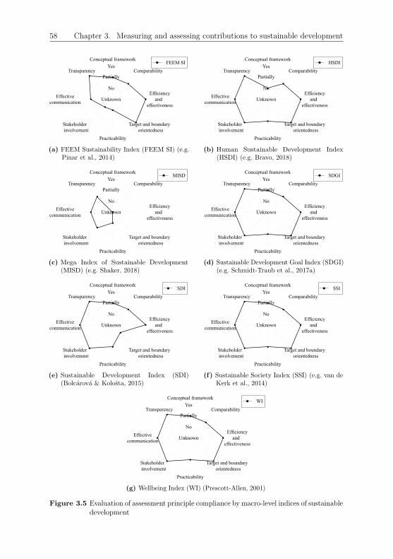
58 Chapter 3. Measuring and assessing contributions to sustainable development
Unknown
No
Partially
YesConceptual framework
Transparency
Effective communication
Stakeholder involvement
Practicability
Target and boundary orientedness
Efficiency and
effectiveness
Comparability●
●
●
●
●
●
●
●
● FEEM SI
(a) FEEM Sustainability Index (FEEM SI) (e.g.Pinar et al., 2014)
Unknown
No
Partially
YesConceptual framework
Transparency
Effective communication
Stakeholder involvement
Practicability
Target and boundary orientedness
Efficiency and
effectiveness
Comparability
●
●
●
●●
●
●
●
● HSDI
(b) Human Sustainable Development Index(HSDI) (e.g. Bravo, 2018)
Unknown
No
Partially
YesConceptual framework
Transparency
Effective communication
Stakeholder involvement
Practicability
Target and boundary orientedness
Efficiency and
effectiveness
Comparability
●
●
●
●
●
●●●
● MISD
(c) Mega Index of Sustainable Development(MISD) (e.g. Shaker, 2018)
Unknown
No
Partially
YesConceptual framework
Transparency
Effective communication
Stakeholder involvement
Practicability
Target and boundary orientedness
Efficiency and
effectiveness
Comparability●
●
●
●●
●
●
●
● SDGI
(d) Sustainable Development Goal Index (SDGI)(e.g. Schmidt-Traub et al., 2017a)
Unknown
No
Partially
YesConceptual framework
Transparency
Effective communication
Stakeholder involvement
Practicability
Target and boundary orientedness
Efficiency and
effectiveness
Comparability●
●
●
●●
●
●
●
● SDI
(e) Sustainable Development Index (SDI)(Bolcarova & Kolosta, 2015)
Unknown
No
Partially
YesConceptual framework
Transparency
Effective communication
Stakeholder involvement
Practicability
Target and boundary orientedness
Efficiency and
effectiveness
Comparability●
●
●
●●
●
●
●
● SSI
(f) Sustainable Society Index (SSI) (e.g. van deKerk et al., 2014)
Unknown
No
Partially
YesConceptual framework
Transparency
Effective communication
Stakeholder involvement
Practicability
Target and boundary orientedness
Efficiency and
effectiveness
Comparability●
●
●
●●
●
●
●
● WI
(g) Wellbeing Index (WI) (Prescott-Allen, 2001)
Figure 3.5 Evaluation of assessment principle compliance by macro-level indices of sustainabledevelopment

3.3. Sustainable development indicators 59
geographical region (see Figure 3.5d). However, its macro-economic focus and resulting
indicator selection prevents it to be applicable to micro and meso objects. Efficiency as
well as effectiveness are measured, targets are included in terms of the SDG agenda or
top five performers, and the transparent presentation enables stakeholder involvement
as well as effective communication.
The SDI aims to quantify a country’s contribution to macro-level sustainable de-
velopment. It includes 12 indicators in areas such as socio-economic development,
sustainable consumption and production, social inclusion, demographic changes, public
health, climate change and energy, sustainable transport, natural resources, and global
partnership (Bolcarova & Kolosta, 2015). The SDI maps the contentual domains of
sustainable development well and is universally applicable to different countries (see
Figure 3.5e). However, given its indicator selection, a computation for micro and
meso objects is not possible, such that comparability across aggregational sizes is not
enabled. Absolute and relative indicators are present, but targets and boundaries
are not included. Its simplicity further ensures practicability (as far as possible, see
Figure 3.2a), stakeholder involvement, and effective communication. The assessment
principle transparency is complied with.
The SSI also aspires to measure macro-level sustainable development of countries,
and contains 21 indicators in the categories basic needs, health, personal and social
development, natural resources, climate and energy, transition, and economy (Saisana
& Philippas, 2012; van de Kerk & Manuel, 2008; van de Kerk et al., 2014). It generally
complies with the conceptual framework by depicting the contentual domains well and
by being universally applicable; scores for 151 countries are computed (see Figure 3.5f).
However, it is only computable for macro objects, and the multilevel perspective is
dismissed. Data and methods are transparently disclosed; targets are included in
terms of a sustainability value, and efficiency as well as effectiveness are included.
Practicability, stakeholder involvement, and effective communication are ensured.
Last, the WI is an index that comprises 87 indicators, thereof 36 indicators that
summarise human wellbeing and 51 indicators that aggregate into ecosystem wellbeing.
Topics covered are health and population, wealth, knowledge and culture, community,
equity, land, water, air, species and genes, and resource use (Mayer, 2008; Prescott-Allen,
2001). The contentual domains of sustainable development are mapped well, but this
index features the same shortcomings as the previously mentioned indices: It is not
compliant with the multilevel perspective, disabling comparability across aggregational
sizes (see Figure 3.5g). However, the WI is in line with the further assessment principles.
Summarising, the review yields following conclusions:
1. Multilevel indices do not exist, and the reviewed indices’ scopes and objectives
disable multilevel applications.
2. If indices encompass the three contentual domains (a prerequisite of this review),
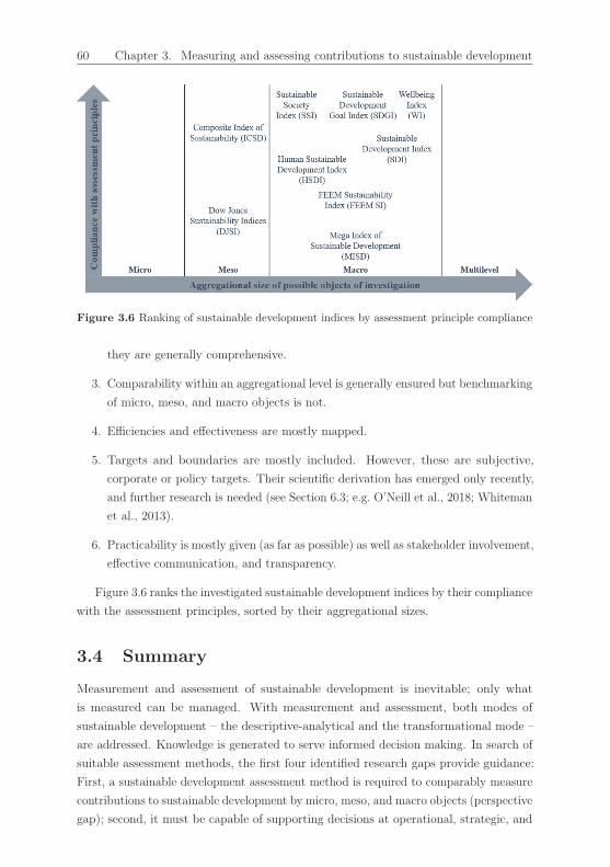
60 Chapter 3. Measuring and assessing contributions to sustainable development
Figure 3.6 Ranking of sustainable development indices by assessment principle compliance
they are generally comprehensive.
3. Comparability within an aggregational level is generally ensured but benchmarking
of micro, meso, and macro objects is not.
4. Efficiencies and effectiveness are mostly mapped.
5. Targets and boundaries are mostly included. However, these are subjective,
corporate or policy targets. Their scientific derivation has emerged only recently,
and further research is needed (see Section 6.3; e.g. O’Neill et al., 2018; Whiteman
et al., 2013).
6. Practicability is mostly given (as far as possible) as well as stakeholder involvement,
effective communication, and transparency.
Figure 3.6 ranks the investigated sustainable development indices by their compliance
with the assessment principles, sorted by their aggregational sizes.
3.4 Summary
Measurement and assessment of sustainable development is inevitable; only what
is measured can be managed. With measurement and assessment, both modes of
sustainable development – the descriptive-analytical and the transformational mode –
are addressed. Knowledge is generated to serve informed decision making. In search of
suitable assessment methods, the first four identified research gaps provide guidance:
First, a sustainable development assessment method is required to comparably measure
contributions to sustainable development by micro, meso, and macro objects (perspective
gap); second, it must be capable of supporting decisions at operational, strategic, and
3.4. Summary 61
normative tier (operational-to-normative gap); third, it is demanded to investigate
interlinkages of the individual sustainable development elements (knowledge gap);
and fourth, it must be easily applicable to put the crafted knowledge into practice
(sustainability gap). To be able to systematically determine a method’s potential in
approaching these gaps, sustainable development assessment principles are reviewed first.
By summarising and harmonising this review, ten assessment principles are yielded:
compliance with framework; comparability in all sustainable development dimensions;
synergies and trade-offs of interconnected themes and goals; efficiency and effectiveness
of impacts; target and boundary orientedness of individual sustainable development
elements; practicability for decision makers; stakeholder involvement for legitimacy;
effective communication to stakeholders; transparency of data, methods, and results;
and methodological soundness. Second, multilevel assessment methods are evaluated
based on these principles. Indicator sets that include a weighted composite indicator
(i.e. a sustainable development index) result to be the most successful assessment
method in tackling the first four identified research gaps. Two meso-level and seven
macro-level indices are identified: the DJSI, ICSD, FEEM SI, HSDI, MISD, SDGI,
SDI, SSI, and the WI. Examining these indices, substantial lacks in the assessment
principles are ascertained. These involve, for instance, the non-comprehensive depiction
of sustainable development elements, the violation of societal instrumental finality,
and lacks in transparency. Moreover, multilevel indices could not be identified in
the literature despite their compelling necessity, demonstrating the expansion of the
perspective gap, which regards the conceptual framework, into methods and empirical
findings. The multilevel perspective is neglected in the conceptual framework, leading to
an absence of multilevel indices. This in turn results in a lack of multilevel comparable
empirical findings. Given these deficiencies, this work develops a new index – the
MLSDI – that comparably measures multilevel contributions to sustainable development,
supports decisions at all tiers, comprehensively studies interconnections of sustainable
development elements, and is applicable in practice. The MLSDI’s methodology follows
in the next chapter, Chapter 4.

62 Chapter 3. Measuring and assessing contributions to sustainable development
Open Access This chapter is licensed under the terms of the Creative Commons At -tribution 4.0 International License (http://creativecommons.org/licenses/by/4.0/), which permits use, sharing, adaptation, distribution and reproduction in any medium or format, as long as you give appropriate credit to the original author(s) and the source, provide a link to the Creative Commons license and indicate if changes were made.
The images or other third party material in this chapter are included in the chapter’s Creative Commons license, unless indicated otherwise in a credit line to the mate-rial. If material is not included in the chapter’s Creative Commons license and your intended use is not permitted by statutory regulation or exceeds the permitted use, you will need to obtain permission directly from the copyright holder.
Chapter 4
Methodology
Because sustainable development only becomes defined when measured (see Chapter 3;
e.g. Bell & Morse, 2008), sustainable development index construction is an unsupervised
modelling task without a supervising output variable (G. James, Witten, Hastie &
Tibshirani, 2013). Consequently, sustainable development measurement is diverse
in methods and methodologies (see Section 3.2, Section 3.3, and Section 4.2) and
hallmarked by subjectivity and arbitrariness (e.g. Bohringer & Jochem, 2007), such
that sustainable development indicators are rather confusing and non-consensual (Pope
et al., 2017; Ramos & Moreno Pires, 2013). To counteract this finding and to achieve
objectivity in assessment (see Table 3.1; Sala et al., 2015), the previous theoretical
research is coupled with a profound methodological research. The conceptual framework
derived in Chapter 2 has resulted in assessment principles in Section 3.1, and these now
guide the methodological choices to be made from a pool of alternative techniques for
each index calculation step. Thereby, methodological shortcomings of previous indices
are overcome, which constitute the fifth and last research gap. Moreover, methodological
understanding of the interactions of the individual sustainable development elements
will be established by the end of this chapter: The knowledge gap (see Section 2.3.3;
e.g. Weitz et al., 2018) is addressed by the index computation (see Section 3.2).
The first part of this chapter, Section 4.1, introduces the calculation steps of a
sustainable development index and establishes methodological requirements based on the
assessment principles in Section 3.1. By means of these requirements, the methodological
approaches of the indices identified in Section 3.3.2 and Section 3.3.3 are evaluated
in Section 4.2. The main part of this chapter, Section 4.3, addresses the MLSDI’s
methodology. First, data are collected (see Section 4.3.1), prepared (see Section 4.3.2
and Section 4.3.4), and cleaned (see Section 4.3.3 and Section 4.3.5); second, the major
index computation steps are executed (see Section 4.3.6 to Section 4.3.8); and third,
sensitivities are investigated (see Section 4.3.9). This chapter ends with a summary and
interim conclusion in Section 4.4 that conflate the theoretical investigation of Chapter 2
and Chapter 3 as well as the methodological research of this chapter.
© The Author(s) 2021C. Lemke, Accounting and Statistical Analyses for SustainableDevelopment, Sustainable Management, Wertschöpfung undEffizienz, https://doi.org/10.1007/978-3-658-33246-4_4

64 Chapter 4. Methodology
4.1 Overview of sustainable development indices’
calculation steps and methodological require-
ments
Sustainable development indices are typically constructed in nine steps. These are
visualised in Figure 4.1, and a primer can be found in Nardo et al. (2008). The
first calculation step comprises the collection of sustainable development key figures
(see Section 4.3.1). Key figures are the raw data to collect. For transparency (see
Table 3.1; e.g. Pinter et al., 2018), data acquisition should be open access. The
preparation of sustainable development key figures is realised in the second calculation
step (see Section 4.3.2) and is necessary because data from different aggregational objects
(micro, meso, and macro) must be harmonised for multilevel object comparability (see
Table 3.1; e.g. Hacking & Guthrie, 2008) and methodological soundness in terms of
credibility, validity, and reliability (see Table 3.1; e.g. Cash et al., 2003; Janouskova
et al., 2018). This step is typically not included in sustainable development index
calculations because Rotmans et al.’s (2001; see Section 2.3.1) multilevel perspective
is disregarded (see Section 3.3.2 and Section 3.3.3). Imputation of missing values is
performed (see Section 4.3.3) to turn the key figures’ incomplete data set into a complete
one (van Buuren, 2012), reducing statistical biases (e.g. Little & Rubin, 2002) and
ensuring the assessment principle methodological soundness (see step two). Imputation
is deployed on key figures (i.e. the raw data) in order to prevent possible biases
that would arise from afore-going calculations such as standardisation accomplished
in the next step. Standardisation to sustainable development key indicators is realised
with the complete sample of key figures (see Section 4.3.4). It accounts for different
aggregational sizes of micro, meso, and macro objects of investigation and ensures the
assessment principle multilevel object comparability (see Table 3.1; e.g. Hacking &
Guthrie, 2008). Moreover, the key indicators are primarily in charge of the assessment
principle compliance with framework (see Table 3.1; e.g. Pinter et al., 2018). For
instance, the key indicators critically determine the comprehensiveness (e.g. Bohringer
& Jochem, 2007) and capability of multilevel application of an index because the key
indicators are an index’s data input. Both key figures and key indicators are variables
in terms of input data at certain stages of an index. In this context, Waas et al.’s (2014;
see Section 3.3) finding that a variable becomes an indicator when linked to a reference
value is disregarded. In order to prevent misunderstandings, the term “variable” is only
used in general contexts of a method’s input data, and when referring to input data of
a sustainable development index, “key figure” or “key indicator” is quoted, respectively.
Furthermore, a methodologically sound index only contains relevant key indicators (see
Table 3.1; Janouskova et al., 2018) and maps both efficiencies and effectivenesses of
sustainable development performances (see Table 3.1; e.g. Figge & Hahn, 2004).
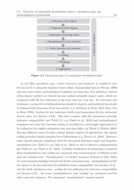
4.1. Overview of sustainable development indices’ calculation steps andmethodological requirements 65
Figure 4.1 Calculation steps of a sustainable development index
In the fifth calculation step, outlier detection and treatment is conducted (see
Section 4.3.5) to diminish statistical biases (Hadi, Rahmatullah Imon & Werner, 2009)
and once more induce methodological soundness (see step two). Key indicators’ instead
of key figures’ outliers are treated because outliers primarily impact scales, which are
computed with the key indicators in the next step (see step six). For detection and
treatment, a perspective of information loss should be adopted, and statistical bias should
be balanced with distortion of the true picture (e.g. McGregor & Pouw, 2017; Zhou, Fan
& Zhou, 2010). Scaling the key indicators (sixth step) harmonises the key indicators’
diverse units (see Section 4.3.6). This step complies with the assessment principle
indicator comparability (see Table 3.1; e.g. Pinter et al., 2018) and methodological
soundness (see step two) because scaling is essential for a meaningful aggregation to
be realised in the eighth calculation step (see step eight; e.g. Ebert & Welsch, 2004).
Because different types of scales contain distinct degrees of information, the chosen
scaling procedure should minimise loss of information (e.g. Zhou et al., 2010). Moreover,
scales should empower compliance with the assessment principles target and boundary
orientedness (see Table 3.1; e.g. Sala et al., 2015) as well as effective communication
(see Table 3.1; e.g. Pinter et al., 2018). A further clarification of terminology is required:
Both standardisation and scaling are concerned with transformation of different scales
onto one common scale. “Normalisation” is a further synonym (Pollesch & Dale, 2016).
To avoid misunderstandings between the fourth calculation step – standardisation of the
key figures to the key indicators for multilevel object comparability (see Section 4.3.4) –
and the sixth calculation step – scaling the key indicators for indicator comparability
(see Section 4.3.6) – the terms “standardisation” and “scaling” are exclusively used for
their respective purposes. The expression “normalisation” remains unused.

66 Chapter 4. Methodology
Figure 4.2 Layers of an overall sustainable development index
The seventh calculation step accomplishes weighting of scaled key indicators (see
Section 4.3.7). This step is essential for assessing relationships among the data (e.g.
Greco, Ishizaka, Tasiou & Torrisi, 2019) and accounting for synergies and trade-offs (see
Table 3.1; e.g. Costanza, Fioramonti & Kubiszewski, 2016). Thereby, it is the substantive
step in closing the knowledge gap (see Section 2.3.3; e.g. Weitz et al., 2018). In doing
so, methodological soundness in terms of objectivity (see Table 3.1; Sala et al., 2015)
and relevance should be guaranteed (see Table 3.1; Janouskova et al., 2018). The eighth
step performs aggregation (see Section 4.3.8). First, scaled and weighted key indicators
are aggregated into sustainable development subindices of each contentual domain.
Second, these are combined to an overall sustainable development index. Figure 4.2
visualises the layers of an overall sustainable development index. The implemented
aggregation function moderates the degree of substitutability (Grabisch, Marichal,
Mesiar & Pap, 2009) and is hence guided by the allowance of weak sustainability with
minimised substitutability within the safe and just operating space for humanity (see
Section 2.2.4). Furthermore, the aggregation function must interplay meaningfully
with the underlying scales for methodological soundness (see step six; e.g. Ebert &
Welsch, 2004) and also minimise loss of information (e.g. Zhou et al., 2010). Last,
sensitivity analyses are carried out for calculation steps that provide alternatives (see
Section 4.3.9). The aim is to ensure methodological soundness in terms of credibility,
validity, reliability, and robustness (see Table 3.1; e.g. Cash et al., 2003; Janouskova
et al., 2018; Sala et al., 2015) and enhance transparency (see Table 3.1; e.g. Pinter
et al., 2018). In case of the MLSDI sensitivities are tested for missing value imputation,
outlier detection, and weighting. For the other calculation steps, the theoretical and
methodological research points to one unique approach.
Methodological soundness is emphasised in individual calculation steps despite being
effective in each step and the overall computation. Table 4.1 provides a summary of the

4.2. Methodological evaluation of sustainable development indices 67
Calculation step Guiding assessment principle and further cri-teria
1. Collection of key figures Transparency
2. Preparation of key fig-ures
Multilevel object comparability, methodolo-gical soundness (credibility, validity, reliabil-ity)
3. Imputation of missingvalues
Methodological soundness (see step two)
4. Standardisation to keyindicators
Comprehensiveness, multilevel object com-parability, methodological soundness (relev-ance), efficiency and effectiveness
5. Outlier detection andtreatment
Methodological soundness (see step two), bal-anced information loss
6. Scaling Indicator comparability, methodologicalsoundness (see step two), minimum informa-tion loss, target and boundary orientedness,effective communication
7. Weighting Synergies and trade-offs, methodologicalsoundness (objectivity, relevance)
8. Aggregation Weak sustainability with minimised substi-tutability, methodological soundness (seestep two), minimum information loss
9. Sensitivity analyses Methodological soundness (credibility, valid-ity, reliability, robustness), transparency
Table 4.1 Assignment of the guiding assessment principles and further criteria to the calcu-lation steps of a sustainable development index
assignment of the guiding assessment principles and further criteria to the calculation
steps of a sustainable development index. Based on this assignment, methodological
approaches of the nine identified sustainable development indices (see Section 3.3.2 and
Section 3.3.3) are evaluated in the following section, Section 4.2. In contrast to the
indices’ evaluation in Section 3.3.2 and Section 3.3.3, methodological soundness and
the assessment principles’ connection to an index’s major calculation steps – step six to
step nine – are focused on.
4.2 Methodological evaluation of sustainable devel-
opment indices
The first evaluated index in Section 3.3.2 is the family of DJSI (e.g. S&P Dow Jones
Indices, 2018, 2019). It has been concluded that the DJSI are not presented transparently.
In this vein, data cleaning (missing value imputation and outlier treatment), sensitivity

68 Chapter 4. Methodology
Unknown
No
Partially
YesSound data cleaning
Sensitivity analyses
Sound aggregation
Sound weighting
Sound scaling
●●●
●
●
● DJSI
(a) Dow Jones Sustainability Indices (DJSI) (e.g.S&P Dow Jones Indices, 2018)
Unknown
No
Partially
YesSound data cleaning
Sensitivity analyses
Sound aggregation
Sound weighting
Sound scaling●
●
● ●
●
● ICSD
(b) Composite Sustainable Development Index(ICSD) (Krajnc & Glavic, 2005)
Figure 4.3 Evaluation of methodological soundness and linkage to assessment principles bymeso-level indices of sustainable development
analyses, scaling, and aggregation are unknown. Full information on weighting is not
provided, but it is announced that weights are floating and industry specific. Individual
weight adjustment should be refrained from because it disables comparability (see
Section 4.3.6.2; Nardo et al., 2008) and grants developers mediating power, setting
low weights on underperforming elements (see Section 3.2; Jesinghaus, 2018). The
evaluation of the DJSI’s methodological soundness and major calculation steps’ linkage
to assessment principles is portrayed in Figure 4.3a.27
The other identified micro-level sustainable development index is the ICSD (Krajnc
& Glavic, 2005). It does not impute missing values, treat outliers, nor does it test
sensitivities (see Figure 4.3b). Data cleaning might be superfluous because of the small
sample size, but a holistic methodological approach prepares for occasions in which data
cleaning becomes necessary (Nardo et al., 2008). Scaling is accomplished by ratio scaling
with target setting. Key indicators are divided by company targets, implementing the
assessment principle target and boundary orientedness. However, ratio scaling entails
mathematical inconsistencies (see Section 4.3.6.2; Pollesch & Dale, 2016), and scores
are difficult to interpret, such that effective communication is harmed. Weights are
determined by the analytical hierarchy process, which involves critical subjectivities
(see Section 4.3.7.1; Zhou, Ang & Poh, 2006). Arithmetic aggregation is applied, but
this aggregation function is not compatible with the underlying scales, leading to
meaningless results (see Section 4.3.8; e.g. Ebert & Welsch, 2004). Moreover, arithmetic
aggregation implements weak sustainability but does not minimise substitutability (see
Section 4.3.8; e.g. Pollesch & Dale, 2015).
Among the identified macro-level indices, the FEEM SI is the first index to be
examined (e.g. Pinar et al., 2014). Missing values are not imputed, but outliers are
treated with lower weights (see Figure 4.4a). Compared to a non-treatment, this
procedure is progressive, but biases remain (see Section 4.3.5.2; Rassler, Rubin & Zell,
27References and sources of the assessment principles are not repeated in this section but can befound in Section 3.1, Section 4.1, and Section 4.3.

4.2. Methodological evaluation of sustainable development indices 69
2013). Policy targets are included in the scaling procedure, which is performed by
rescaling. The data range on a discrete interval from zero to one. Rescaling yields easily
understandable scores, encouraging effective communication. However, scales should
be continuous to minimise information loss (see Section 4.3.6 and Section 4.3.7.4; e.g.
Yang & Webb, 2009; Zhou et al., 2010). Weights are determined by experts’ elicitation,
and aggregation relies on the Choquet integral, which allows for preference-based
index construction. Both experts’ elicitation and Choquet integral do not follow the
assessment principle objectivity. Notwithstanding, sensitivities of experts’ preferences
are tested.
The HSDI does not clean data, nor does it test sensitivities (see Figure 4.4b; e.g.
Bravo, 2018). Equal weights are applied, ignoring correlations of indicators. Equally
weighted correlated variables entail double counting of the correlated information,
implicitly upgrading their weights (see Section 4.3.7.1; Greco et al., 2019; Nardo et al.,
2008). Hence, equal weights are “universally considered to be wrong” (see Section 4.3.7.1;
e.g. Chowdhury & Squire, 2006). Data are scaled between zero and one and aggregated
geometrically. Geometric aggregation implements weak sustainability with minimised
substitutability (see Section 4.3.8; e.g. Pollesch & Dale, 2015). However, it obtains
overall zero results when combined with a lower rescaling bound of zero. In other words,
substitutability vanishes, and thus, the lower bound should be raised (see Section 4.3.6.2
and Section 4.3.8; Saisana & Philippas, 2012).
The MISD comprises 31 indices (e.g. Shaker, 2018). Therefore, an overall methodo-
logical evaluation is not feasible. Concentrating on the MISD, it does not treat outliers
despite recognising issues in computation (see Figure 4.4c). However, it overcomes other
indices’ methodological shortcomings in terms of missing value imputation: The MISD
fills missing values by multiple imputation, reducing statistical biases (see Section 4.3.3;
e.g. Little & Rubin, 2002) and accounting for uncertainties in the imputation process
(see Section 4.3.3.3; e.g. Schafer & Graham, 2002). Furthermore, it determines weights
by multivariate statistical analysis, which is generally the preferred field of methods (see
Section 4.3.7.1; Mayer, 2008). However, factor analysis is not suitable for sustainable
development index construction because it is a top-down approach (see Section 4.3.7.1;
Haerdle & Simar, 2012). Similar to the HSDI, rescaling between zero and one is
combined with geometric aggregation. Sensitivities are not investigated.
The SDGI does not treat missing values on purpose in order to draw attention
to missing data. Although, few exceptions carried out cold deck or mean imputation
(see Figure 4.4d; Schmidt-Traub et al., 2017b). Both methods do not fully eliminate
statistical biases (see Section 4.3.3.2; Rassler et al., 2013). The SDGI claims to follow
Nardo et al.’s (2008)28 recommendation “truncating the data by removing the bottom
2.5 percentile from the distribution” (Schmidt-Traub et al., 2017b). Replacing outliers
28Schmidt-Traub et al. (2017b) reference a 2016 publication. To the best of the author’s knowledge,the here cited 2008 publication by Nardo et al. is the most recent one at the time of research.

70 Chapter 4. Methodology
Unknown
No
Partially
YesSound data cleaning
Sensitivity analyses
Sound aggregation
Sound weighting
Sound scaling
●
●
● ●
●
● FEEM SI
(a) FEEM Sustainability Index (FEEM SI) (e.g.Pinar et al., 2014)
Unknown
No
Partially
YesSound data cleaning
Sensitivity analyses
Sound aggregation
Sound weighting
Sound scaling●
●
●
●
●
● HSDI
(b) Human Sustainable Development Index(HSDI) (e.g. Bravo, 2018)
Unknown
No
Partially
YesSound data cleaning
Sensitivity analyses
Sound aggregation
Sound weighting
Sound scaling
●
●
●
●
●
● MISD
(c) Mega Index of Sustainable Development(MISD) (e.g. Shaker, 2018)
Unknown
No
Partially
YesSound data cleaning
Sensitivity analyses
Sound aggregation
Sound weighting
Sound scaling
●
●
● ●
●
● SDGI
(d) Sustainable Development Goal Index (SDGI)(e.g. Schmidt-Traub et al., 2017b)
Unknown
No
Partially
YesSound data cleaning
Sensitivity analyses
Sound aggregation
Sound weighting
Sound scaling
●
●
●
●
●
● SDI
(e) Sustainable Development Index (SDI)(Bolcarova & Kolosta, 2015)
Unknown
No
Partially
YesSound data cleaning
Sensitivity analyses
Sound aggregation
Sound weighting
Sound scaling
●
●
●
●
●
● SSI
(f) Sustainable Society Index (SSI) (e.g. van deKerk et al., 2014)
Unknown
No
Partially
YesSound data cleaning
Sensitivity analyses
Sound aggregation
Sound weighting
Sound scaling
●
●
● ●
●
● WI
(g) Wellbeing Index (WI) (Prescott-Allen, 2001)
Figure 4.4 Evaluation of methodological soundness and linkage to assessment principles bymacro-level indices of sustainable development

4.2. Methodological evaluation of sustainable development indices 71
with thresholds is methodologically sound, but Nardo et al. (2008) advises to shorten
the bottom and top of a distribution; one-sided treatment is not reasonable (see
Section 4.3.5.2). Rescaling between zero and 100 is appropriate in the context of
arithmetic aggregation. However, the arithmetic mean should be avoided and likewise
should equal weights (see above). Sensitivities are tested for outlier thresholds and the
aggregation function.
The SDI does not treat outliers, nor does it investigate sensitivities (see Figure 4.4e;
Bolcarova & Kolosta, 2015). It imputes missing values, but the chosen mean imputation
still leads to invalid inferences (see Section 4.3.3.2; Rassler et al., 2013). Sound
weighting is executed by application of multivariate statistical analysis. In particular,
the bottom-up Principal Component Analysis (PCA) is deployed (see Section 4.3.7.1
and Section 4.3.7.2; e.g. Mayer, 2008). Classical scaling and aggregation in PCA are
z-scores (mean equal to zero and variance equal to one) and arithmetic aggregation.
Both are retained in the SDI. Arithmetic aggregation does not fulfil the methodological
criteria (see above). Z-scores are not favourable because they are difficult to interpret,
and due to negative values, they cannot be combined with geometric aggregation (see
Section 4.3.6.2; e.g. Field, 2009).
The SSI imputes missing values by expert judgement (e.g. van de Kerk et al.,
2014). Compared to a non-imputation case, bias is reduced, but the assessment
principle objectivity is violated (see Figure 4.4f). Outliers are identified with thresholds
on skewness and kurtosis and treated by non-linear scale transformations. Both
methods are not recommendable. First, skewness and kurtosis are not robust to outliers
because outliers inflate these measures, such that outliers might not be detected as
such (see Section 4.3.5.2; e.g. Aggarwal, 2017; Hadi et al., 2009). Second, non-linear
transformation is particularly harmful in index calculation because it changes correlations
between variables (see Section 4.3.5.2; Oh & Lee, 1994), while correlations should be
investigated in statistical weighting procedures (see Section 4.3.7.1; e.g. Mayer, 2008).
The SSI does not deploy statistical but top-down equal weighting. On the positive side,
the non-linear transformations are not harmful because correlations are not investigated.
On the other side, equal weights are not sufficient (see above). Furthermore, the
justification of the SSI to implement equal weighting because “[t]here are no highly
correlated indicators (all Pearson correlations coefficients are lower than 0.82)” (Saisana
& Philippas, 2012) might be false: Correlation coefficients greater than 0.8 typically
indicate very high correlations (Field, 2009). Apart from that, Pearson’s coefficient
might be inappropriate because it assumes normality (see Section 4.3.3.3; Field, 2009),
which is not tested in the SSI. Nonetheless, sound scaling, sound aggregation, and
sensitivity analyses are executed: Geometric aggregation is applied on the rescaled
indicators, and sensitivities are tested for the weighting procedure. The rescaling range
starts at one and ends at ten; substitutability is maintained throughout the entire range.
The WI partially deals with missing values, but the method remains unknown (see

72 Chapter 4. Methodology
Figure 4.4g; Prescott-Allen, 2001). Outliers are detected and replaced by respective
threshold values. However, the detection is one-sided (at the top). Weighting is arbitrary,
arithmetic aggregation is applied, and sensitivities are not tested. On the positive side,
rescaling between zero and 100 is implemented.
In conclusion, previous sustainable development indices do not only lack compliance
with the assessment principles (see Section 3.3.2 and Section 3.3.3) but fail to meet
methodological and scientific requirements (see above; e.g. Bohringer & Jochem, 2007).
This forms the fifth and last research gap. Major criticisms include non-comprehensive
scope (das Neves Almeida, Cruz, Barata & Garcıa-Sanchez, 2017; Frugoli, Villas Boas
de Almeida, Agostinho, Giannetti & Huisingh, 2015; Singh et al., 2012); insufficient
weighting, not addressing interconnections of indicators (i.e. knowledge gap; see
Section 2.3.3; e.g. Weitz et al., 2018); meaningless aggregation; missing sensitivity
analyses (Bohringer & Jochem, 2007; Singh et al., 2012); and statistical biases as a
result of unsatisfactory data cleaning.
To overcome these conceptual and methodological shortcomings, the following
section, Section 4.3, conducts profound methodological research on each calculation
step of a sustainable development index. The MLSDI’s methodology will be the result.
4.3 Methodology of the Multilevel Sustainable De-
velopment Index (MLSDI)
This section addresses each calculation step of a sustainable development index in detail
and derives the MLSDI. On that account, broad methodological research is carried
out, and a variety of methods are reviewed to make profound decisions. This section’s
structure follows the nine calculation steps (see Figure 4.1).
4.3.1 Collection of sustainable development key figures
The first step in the calculation process is the collection of sustainable development key
figures. These are inferred from the sustainable development key indicators, and further
information will follow in Section 4.3.4. Decisive in the key figure collection process
is data availability: Data must be available by official statistics. Official statistics are
open access and hence easily acquired (Zuo, Hua, Dong & Hao, 2017), addressing the
sustainability gap (see Section 2.3.4; e.g. Hall et al., 2017) and ensuring the assessment
principle transparency (see Table 3.1; e.g. Pinter et al., 2018).
The structure of the set of sustainable development key figures c5 follows from the
conceptual framework (see Chapter 2) and is formally denoted by:
c5 = c5(n, x, t, r), (4.1)

4.3. Methodology of the Multilevel Sustainable Development Index (MLSDI) 73
Figure 4.5 Structure of the sustainable development key figures’ data set
where nε[1, N ] represents an economic object of the change agent group business of
any aggregational size, xε[1, X] portrays a sustainable development key figure, tε[1, T ]
depicts a time period, and rε[1, R] is a geographical region. The structure of the set
of key figures c5 is illustrated in Figure 4.5. Economic objects n are stored in rows,
columns contain key figures x, tables represent time periods t, and geographical regions
r constitute the fourth axis.
Neither society, policy, nor science are objects of investigation but participate in
the transition to sustainability by, for instance, designing, performing, or drawing
conclusions on the analysis (see Section 3.2). Moreover, as a consequence of the
multilevel perspective, economic objects n are organised in an inclusive hierarchy :
Multiple layers are nested within each other (Steenbergen & Jones, 2002), and higher
ranked economic objects n contain lower ranked economic objects n. That is, macro-
economic objects n such as conglomerates of institutions or organisations comprise
meso-economic objects n such as networks, communities, or organisations, and these in
turn encompass micro-economic objects n such as individuals and individual actors (see
Section 2.3.1; Rotmans et al., 2001). In contrast, in an exclusive hierarchy, objects that
are ranked lower are not included in objects that are ranked higher (Gibson, Ostrom &
Ahn, 2000). To avoid complex multilevel methods, which implicitly account for double
counts arising from the inclusive hierarchy, the inclusive hierarchical multilevel data
structure is eliminated before the MLSDI’s modelling process. Section 5.1 will reveal
that the industry level is maintained, while potential corporations, aggregated branches,
or overall economies are eliminated. Bias from the elimination is not expected because
of the inclusiveness. Not potential corporations at the meso level but industries at the

74 Chapter 4. Methodology
macro level are maintained because sustainable development is a macro-level concept
(see Section 2.3.2; e.g. T. Hahn et al., 2015).
The following section, Section 4.3.2, describes the preparation of key figures x.
4.3.2 Preparation of sustainable development key figures
The key figures’ preparation homogenises data formats to enable multilevel comparability
and to accomplish the assessment principle methodological soundness in terms of
credibility, validity, and reliability (see Table 3.1; e.g. Cash et al., 2003; Janouskova
et al., 2018). With respect to multilevel comparability, meso-economic company data
are transferred to macro-economic categories (see Section 4.3.2.1). A transfer from meso
to macro and not vice versa is performed because economic objects n at the macro
level (i.e. industries) are maintained (see Section 4.3.1). In Section 4.3.2.2, statistical
classifications of macro-economic data are transformed because not all data are released
in the same classification scheme. For both transformations, it is anticipated that
Germany is the sample region r (see Section 5.1) and that data are acquired from the
Statistical Office of the European Communities (Eurostat) and the Federal Bureau
of Statistics (Destatis). The implemented transformation methods in this work are
equivalent to the approaches by the statistical offices.
4.3.2.1 Meso-level transformation to macro-economic categories
Typically, corporations report revenues, costs, and profits, while the macro-economic
Gross Value Added (GVA) is required for standardisation of the key figures x. This
finding is derived in Section 4.3.4. To allow for the demanded standardisation, meso-
economic data is transferred to the GVA, which “is a measure of the contribution to
GDP made by an individual producer, industry or sector” (EC et al., 2009). It can
be calculated in several ways. Computation via the gross and net output is shown
in Table 4.2.29 Another way of calculation is to first determine the intermediate
consumption or input (marked with “†” in Table 4.2) and subsequently subtract it
from the gross output. The output measures all goods and services produced and
not used up by the same establishment, while the intermediate consumption or input
comprises goods and services used up in the production process (EC et al., 2009).
Further definitions can be found in Destatis (2019c); and EC et al. (2009).
4.3.2.2 Macro-level transformation of statistical classifications
This section deals with transformations of official statistical classifications. In the EU and
hence in Germany, official macro-economic statistical data are released in Classification
of Products by Activity (CPA) or Statistical Classification of Economic Activities in
29Publications in German from Destatis are utilised because, in contrast to methodological aspects,meso-economic data collection is decentralised in the European Union (EU).

4.3. Methodology of the Multilevel Sustainable Development Index (MLSDI) 75
+ Revenue of own production
+ Revenue of merchandise
+ Commission fees from trade intermediation
+ Revenue from other, non-industrial activities
− Stock of unfinished and finished goods and services from own productionat the beginning of a period
+ Stock of unfinished and finished goods and services from own productionat the end of a period
+ Self-produced equipment
= Gross output
− Stock of raw materials and supplies at the beginning of a period†
+ Stock of raw materials and supplies at the end of a period†
− Receipt of raw materials and supplies†
− Stock of merchandise at the beginning of a period†
+ Stock of merchandise at the end of a period†
− Receipt of merchandise†
− Cost of subcontractors†
= Net output
− Costs of temporary agency workers†
− Cost of other industrial services†
− Costs of leases and rents†
− Other costs†
= Gross Value Added (GVA)
Table 4.2 Calculation of the Gross Value Added (GVA) with meso-economic data (Destatis,2019c); †, intermediate consumption
the European Community (NACE) (Eurostat, 2008a, 2008b). The first classification
scheme classifies products, and the latter groups industries, which typically produce
more than one product. For the analysis of sustainable development performances by
macro-economic objects n, both classifications are valid. However, because companies
usually produce various products that belong to more than one CPA class, meso-
economic corporate data are generally classified according to NACE. A company’s
NACE assignment is accomplished according to its main field of activity (Destatis,
2019c). Therefore, data classified according to NACE are prerequisites for multilevel
comparability (see Section 4.3.4) that is methodologically sound.
Some official macro-economic statistical data are released in CPA, such that trans-
formations from CPA to NACE are necessary. This is undertaken by methods deployed

76 Chapter 4. Methodology
in the calculation of input-output tables. Input-output tables are symmetric matrices
that serve to present the process of production, use of goods and services, as well
as the income generated (Eurostat, 2008a).30 They are transformations of supply
and use tables, and both contain products in CPA in their rows and industries in
NACE in their columns. Transforming supply and use tables to input-output tables
either yields industry-by-industry or product-by-product tables. Destatis computes
product-by-product tables with the product technology assumption (Destatis, 2010a).
This assumption states that “[e]ach product is produced in its own specific way, irre-
spective of the industry where it is produced” (Eurostat, 2008a). In the computation
process, secondary products are relocated to industries, such that they become primary
products. Primary products are products that are related to one industry by defini-
tion (Eurostat, 2008a). For input-output tables, these are diagonal elements, whereas
secondary products are off-diagonal elements. The technology matrix MT realises the
transformation of classifications and reads:
MT =((I · S)−1 · S)t, (4.2)
where I is an identity matrix, and S depicts a symmetric supply table. Due to
the transposition, the technology matrix MT contains industries in the rows and
products in the columns. To complete the transformation, the technology matrix MT
is multiplied with a sustainable development key figure in CPA xCPA, yielding the
respective sustainable development key figure in NACE xNACE:
xNACE(n, t, r) = MT · xCPA(n, t, r). (4.3)
The set of sustainable development key figures in NACE cNACE5 is represented by:
cNACE5 = cNACE
5 (n, xNACE, t, r). (4.4)
For the remainder of this work, key figures in NACE xNACE are regarded but simply
denoted by “x”. Their set is also simply quoted by “c5”.
On this data set, missing values are imputed as described in the following section,
Section 4.3.3.
4.3.3 Imputation of missing values
Missing values or missing data are underlying but unobserved data (Rassler et al., 2013).
Assuming that missing values are meaningful for the modelling and analysis process,
30Eurostat’s (2008a) Manual of supply, use and input-output tables was released under the EuropeanSystem of Accounts (ESA) 1995. The currently valid standard is ESA 2010 (Eurostat, 2013). Anupdated manual has not been released at the time of research. However, the utilised method is expectedto remain valid without changes under the updated standard.
4.3. Methodology of the Multilevel Sustainable Development Index (MLSDI) 77
they cause a bias if they remain untreated: The observed data dominate the result
(Little & Rubin, 2002). As missing data frequently occur in sustainable development
quantification (e.g. Schmidt-Traub et al., 2017a), dealing with them is an essential step,
contributing to the methodological soundness of an index in terms of credibility, validity,
and reliability (see Table 3.1; e.g. Cash et al., 2003; Janouskova et al., 2018). Generally,
there are four approaches to address missing values, converting the incomplete sample
to a complete one (van Buuren, 2012): complete case analyses, weighting procedures,
model-based procedures, and imputation-based procedures. Complete case analyses
ignore objects with missing data, weighting procedures weight non-response objects less,
model-based procedures specify a model with the observed data, and last, imputation-
based procedures estimate missing values (Little & Rubin, 2002; Rassler et al., 2013).
Generally, only model-based and imputation-based procedures yield valid inferences
(Rassler et al., 2013). Imputation is chosen to handle missing values because it does
not require modelling that is specific to the missing data; this would lead to a loss of
generality in application.
This section is structured as follows. First, missing values are characterised (see
Section 4.3.3.1). Second, two imputation methods are presented: The MLSDI’s single
imputation method is derived in Section 4.3.3.2, and its multiple imputation method
follows in Section 4.3.3.3. Last, statistical tests of model assumptions are outlined in
Section 4.3.3.4.
4.3.3.1 Characterisation of missing values
Three characteristics of missing values are crucial in determining suitable imputation
methods: the missing data pattern, degree of missingness, and the missing data
mechanism. Themissing data pattern describes the structure of observed and unobserved
data in the data set and can be, for instance, univariate, monotone, or general (Little
& Rubin, 2002). General missingness is also referred to as non-monotone (van Buuren,
2012) or arbitrary (Schafer & Graham, 2002). Figure 4.6 visualises these patterns.
Further patterns can be found in, e.g. Little and Rubin (2002).
The degree of missingness can be analysed according to unit non-response and item
non-response. Unit non-response refers to objects that do not deliver any information.
Item non-response regards an object’s missingness of one or more variables. The rate
of missing values λ is the ratio of unobserved to total data and indicates the severity of
the missing data problem (Rassler et al., 2013; van Buuren, 2012).
The relationship between observed and unobserved data is characterised by the
missing data mechanism. The missing data mechanism can be classified into three types.
First, if data are Missing Completely at Random (MCAR), missingness is independent
of the observed as well as the unobserved data. Second, Missing at Random (MAR)
implies that missingness is independent of the unobserved but depends on the observed

78 Chapter 4. Methodology
(a) Univariate (b) Monotone (c) General, non-monotone, orarbitrary
Figure 4.6 Examples of missing data patterns (based on Little and Rubin, 2002; with friendlypermission of c© 2002 by John Wiley & Sons, Inc. All rights reserved)
data. In both cases, distributions of variables are unaffected by inclusion of the missing
data, such that the same modelling process can be performed. The non-response is
ignorable. Third, Missing Not at Random (MNAR) means that missingness depends
on both the observed and the unobserved data, and distributions are influenced by
the missingness. In this non-ignorable case, the model for the complete data differs
from the incomplete data’s model (Little & Rubin, 2002; Rassler et al., 2013; Rubin,
1976; Schafer & Graham, 2002; van Buuren, 2012). Ignorability and MAR are typical
in practice (Enders, 2010) and therefore assumed for the MLSDI, such that only MAR
methods are researched.
4.3.3.2 Single time series imputation: Various methods depending on the
missing data pattern
Generally, methods for missing value imputation can be divided into single and multiple
imputation. Single imputation methods impute missing values only once, whereas
multiple imputation methods are simulation techniques that compute several plausible
values for the final fill (Rassler et al., 2013). Single imputation does not account for
uncertainties in the imputation process, but multiple imputation does (Little & Rubin,
2002). The MLSDI makes use of both single and multiple imputation methods. Single
imputation methods are expected to yield valid results because the uncertainty of the
imputation process is assumed to be relatively low: Either further data in the time series
or higher aggregational economic objects n of the inclusive hierarchy (see Section 4.3.1)
are observed (see Section 5.2.1). In order to confirm or reject the expectation of
uncertainties having a relatively low effect on the MLSDI’s imputation process, single
imputation is tested against multiple imputation (see Section 4.3.3.3).
Single imputation methods comprise hot deck imputation, substitution, cold deck
imputation, imputation by mean, and (stochastic) regression imputation. In hot deck
imputation, data from similar objects serve to impute missing values. Substitution

4.3. Methodology of the Multilevel Sustainable Development Index (MLSDI) 79
replaces blanks with objects that are not in the initial sample, and cold deck imputation
fills missing values with data from external sources (Little & Rubin, 2002; Nardo et al.,
2008). Mean imputation uses the sample mean for estimating missing values. In regres-
sion imputation, observed data represent independent variable(s) to predict missing,
dependent variable(s) (Little & Rubin, 2002). Hot deck and regression imputation are
single imputation methods that are capable of correctly reflecting variability of the
imputation process (Rassler et al., 2013) and are thus applied in the MLSDI.
Generally, a univariate time series point of view is adopted in the MLSDI’s single
imputation process for two reasons: First, key figures x show stable trends (see e.g.
Figure 5.3), such that time periods t are expected to be reliable predictors; and
second, each economic object n is assumed to feature distinct sustainable development
characteristics with the result that cross sections are expected to be unreliable predictors.
Kalman smoothing on a basic structural time series model fitted by the maximum
likelihood method is the preferred single imputation method because it yields more
stable results than further time series models such as Autoregressive Integrated Moving
Average (ARIMA) models (Harvey, 1989; Kalman, 1960). Additionally, its application
enables imputation of the first time period (Moritz, 2018).
A basic structural time series model regards an observation (i.e. a key figure x) as a
permanent trend component μ, seasonal component γ, and an irregular random noise ε
in time period t. The model is described by the following formula (Harvey, 1989):
x(t) = μ(t) + γ(t) + ε(t). (4.5)
On this model, the Kalman filter is applied. It is a recursive algorithm for estimating
observations based on the available information (Harvey, 1989). The estimation is a
maximum likelihood estimation, and parameters that maximise the likelihood function
are searched for. The Kalman filter assumes normally distributed variables, stationarity
(i.e. time invariant distributional properties) of data, and independent and identically
distributed (i.i.d.) residuals (Greene, 2003; Harvey, 1989). However, Harvey (1989)
asserts the Kalman filter to remain an optimal linear estimator that minimises the
mean square error if the normality assumption is violated.
Kalman smoothing on a basic structural time series model is not applicable to any
missing data pattern but requires a minimum of three observations in a time series.
If there are only two observations, the Stineman algorithm is applied (Moritz, 2018).
The Stineman algorithm features monotonical properties and thus gives smoother
results as, for example, polynomial interpolations (Stineman, 1980). Once again, this
property suits the key figures’ stable trends (see e.g. Figure 5.3). If there is only one
observation in the time series, this value is held constant, and a modified hot deck
imputation is deployed: Data from the same economic object n but other time period
t are imputed. If an economic objects’ total time series is unobserved, the inclusive

80 Chapter 4. Methodology
hierarchy (see Section 4.3.1) is taken advantage of: Key figures x of higher aggregational
economic objects n are always observed, and their key indicators y (see Section 4.3.4)
are computed back to the missing lower aggregational key figures x. This is essentially
equivalent to imputing higher aggregational industry means. Rassler et al. (2013) do
not approve mean imputation. However, the presented modified mean imputation is
expected to obtain valid results because the inclusive hierarchy reduces uncertainty in
the imputation process.
To summarise, the missing data pattern imposes limitations on the applicability of
methods, and four single time series imputation techniques are implemented:
• ≥ 3 observations: Kalman smoothing on a basic structural time series modelfitted by a maximum likelihood estimation,
• 2 observations: Stineman algorithm,
• 1 observation: modified hot deck imputation with the only observation,
• 0 observation: modified mean imputation by computing higher aggregationalkey indicators y (see Section 4.3.4) back to the missing lower aggregational keyfigures x.
The MLSDI’s multiple imputation method is determined in the following section,
Section 4.3.3.3.
4.3.3.3 Multiple panel data imputation: Amelia II algorithm
Multiple imputation is a simulation technique that treats parameters as random rather
than fixed. Thereby, multiple plausible results are rendered possible, and uncertainty
of the imputation process is accounted for by adding random noise (Rassler et al., 2013;
Schafer & Graham, 2002; Schafer & Olsen, 1998). The imputation is accomplished by
random draws from a posterior distribution (Rassler et al., 2013; van Buuren, 2012). The
multiple results are combined into one result; usually by the arithmetic mean (Schafer &
Graham, 2002). The convergence of the algorithm to the posterior distribution depends
on the rate of missing values λ and the number of imputations m. Rubin (1987) shows
that the relative efficiency in convergence of an estimate η equals (Schafer & Graham,
2002; Schafer & Olsen, 1998):
η =
(1 +
λ
m
)−1
.31 (4.6)
Equalising the number of imputations m to the percentage rate of missing values λ
is recommended by van Buuren (2012). Furthermore, multiple imputation methods are
well suited for any missing data pattern (Enders, 2010), and differentiations as in single
imputation (see Section 4.3.3.2) are not required.
31Rubin’s (1987) original formula in units of standard deviations has been adjusted.

4.3. Methodology of the Multilevel Sustainable Development Index (MLSDI) 81
Generally, two modelling types exist in the field of multiple imputation: joint
modelling (e.g. Rubin, 1987; Schafer, 1997) and fully conditional specification (e.g.
van Buuren, 2007; van Buuren, Brand, Groothuis-Oudshoorn & Rubin, 2006). Joint
modelling fills missing data by drawing simultaneously from one joint multivariate
distribution. In contrast, fully conditional specification imputes missing values One-
at-a-Time (OAT) on a series of univariate distributions that are directly specified by
the modeller (Mistler & Enders, 2017; van Buuren, 2012). According to Hughes et al.
(2014); Liu, Gelman, Hill, Su and Kropko (2014); and Mistler and Enders (2017),
joint modelling and fully conditional specification are equivalent under single level
multivariate normal data. In contrast, van Buuren (2012) emphasises better theoretical
properties of joint modelling and advises to prefer this modelling type if the data fulfil
the modelling assumptions and if flexibility of individual specification is not demanded.
In addition to van Buuren’s (2012) argument, joint modelling is preferable for the
MLSDI because multiple panel data imputation is aimed to be tested against single
time series imputation. A joint multivariate distribution is therefore favoured over a
series of univariate distributions.
Several software packages for multiple imputation by joint modelling exist, and
overviews can be found in, e.g. Mistler and Enders (2017); and Yucel (2011). Amelia II
is applied for multiply imputing the MLSDI’s missing data (Honaker, King & Blackwell,
2018). It is the most promising software application in multiple imputation for four
reasons: First, it is the only application that uses an expectation maximisation with
bootstrapping algorithm (see below), second, several prior information can be included,
third, simulation studies provide evidence that Amelia II outperforms other programmes
such as NORM (Blankers, Koeter & Schippers, 2010; Novo & Schafer, 2015; Schafer,
1997), and fourth, its developers claim it to work well under violation of the normality
assumption (Honaker, King & Blackwell, 2011). Non-normal data are likely in index
construction, given the numerous key figures x and key indicators y to include for
comprehensiveness of the index (see Table 3.1 and Section 4.3.4; e.g. Hacking & Guthrie,
2008). However, the last argument should be carefully considered. Demirtas, Freels
and Yucel (2008) show that a violation of normality in multiple imputation produces
biased results in their small sample of size 40. The results are only not distorted for
their large sample of size 400, even with high rates of missing values λ such as 75%.
Amelia II works in three steps: bootstrapping, expectation maximisation, and
imputation. These are repeated m times. Bootstrapping is a random sampling technique
that is faster, more flexible, and easier to use than other techniques such as Markov
chain Monte Carlo approaches (Blankers et al., 2010; Honaker et al., 2011).32 An
expectation maximisation algorithm is a framework for maximum likelihood estimation
and estimates parameters of a predictive distribution function (Han, Kamber & Pei,
32More information on bootstrapping can be found in, e.g. Davison and Hinkley (1998); Efron andTibshirani (1993); and G. James et al. (2013).
82 Chapter 4. Methodology
2012).33 Last, missing values are imputed by drawing from the bootstrapped parameters.
Given the m repetitions, m imputed data sets are at hand and combined into one result
(Honaker et al., 2011, 2018).
For the MLSDI, Amelia II’s panel data model is applied on the set of key figures c5.
As many key figures x as possible are included in the model: Complete key figures x are
generally incorporated, and only highly correlated key figures x are excluded (Honaker
et al., 2011; Rassler et al., 2013). The correlation analysis can be based on three
different correlation coefficients: Pearson’s coefficient, Spearman’s rho, or Kendall’s
tau. Pearson’s coefficient assumes normally distributed data, while Spearman’s rho and
Kendall’s tau are non-parametric statistics without distributional assumptions (Field,
2009). Normality of key figures x is tested (see Section 4.3.3.4 and Section 5.2.2) to
determine the adequate coefficient. Should the data be normal, Pearson’s coefficient
is chosen. Otherwise, Kendall’s tau is calculated because it features better statistical
properties than Spearman’s rho despite being less popular. The threshold for being
highly correlated is set to 0.8 (Field, 2009), boundaries on estimates are equalised to the
observed range of values, time effects are specified to be linear and constant across time
series and cross sections, the number of imputations m is levelled to the percentage
rate of missing values λ, and last, the arithmetic mean is applied to combine the results
(see above; Schafer & Graham, 2002; van Buuren, 2012).
In the following section, Section 4.3.3.4, tests for the underlying assumptions of
both single and multiple imputation are outlined.
4.3.3.4 Statistical tests of model assumptions
The first assumption to be tested of both single and multiple imputation is the MAR
assumption (see Section 4.3.3.1). However, MCAR is the only testable missing data
mechanism as the required information for a MAR or MNAR test is missing (Enders,
2010; van Buuren, 2007). Enders (2010) predicate the impossibility of MAR and MNAR
tests to be an important problem in practice. In contrast, Collins, Schafer and Kam
(2001); Rassler et al. (2013); and Schafer and Graham (2002) assert minor effects
and valid inferences as a result of violating assumptions on missing data mechanisms.
Furthermore, Rassler et al. (2013) recommend MAR methods in any case because they
facilitate the modelling and analysis process while still reducing biases compared to
non-treatment. For the MLSDI, Little’s (1988) MCAR test is performed because a
confirmation of MCAR implies approving MAR. The MCAR test is a multivariate
extension of the t-test, evaluating mean differences across subgroups. Under the null
hypothesis, data are MCAR: The missing data patterns share a common mean, and
the test statistic is approximately χ2 distributed (Beaujean, 2015; Enders, 2010). The
null hypothesis is desired to be accepted, and large p-values, which represent standard
33More information on expectation maximisation algorithms can be found in, e.g. Han et al. (2012);and McLachlan and Krishnan (1997).

4.3. Methodology of the Multilevel Sustainable Development Index (MLSDI) 83
normal probabilities, are demanded. Statistical significance is chosen to occur above
p-values of 0.05. However, the test suffers from low power, and its usefulness is therefore
limited (Enders, 2010).34
Regarding single time series imputation, the three assumptions of the basic structural
time series model – normality, stationarity, and i.i.d. – are tested. The Shapiro-Wilk
and Kolmogorov-Smirnov tests serve to investigate normality (Conover, 1980; CRAN,
2019; Royston, 1982; Shapiro & Wilk, 1965), stationarity is examined by the augmented
Dickey-Fuller test (Dickey & Fuller, 1979, 1981; Trapletti, Hornik & LeBaron, 2018),
and the Ljung-Box test is implemented to control for independence of residuals (CRAN,
2019; Ljung & Box, 1978). The Shapiro-Wilk and Kolmogorov–Smirnov tests are non-
parametric tests that compare variance scores and distribution functions of the sample
to a normal distribution, respectively. Under the null hypothesis, the data are normally
distributed. The null hypothesis is desired to be accepted with p-values larger than
0.05. Tests are performed for every time period t because time is an implicit variable.
For conciseness, the test results are compiled into one result by the arithmetic mean. In
large samples, both tests suffer from type I error (rejection of a true null hypothesis),
and thus, visualisation of the data by, for example, histograms should accompany the
tests (Field, 2009). The augmented Dickey-Fuller test is a likelihood ratio test, and
its null hypothesis states that data are generated by a unit root. That is, data are
non-stationary (Dickey & Fuller, 1979, 1981). Consequently, the null hypothesis is
desired to be rejected with p-values smaller than 0.05 (Greene, 2003). Last, under the
null hypothesis of the Ljung-Box test, residuals are i.i.d. The null hypothesis is desired
to be accepted with p-values larger than 0.05 (Brockwell & Davis, 2016; Ljung & Box,
1978). Both the augmented Dickey-Fuller and Ljung-Box tests refer to the temporal
dimension, and the tests are carried out once for the total time series; compiling test
results is not required.
In the case of the Amelia II algorithm, joint multivariate normality is tested
with the multivariate Shapiro-Wilk test (Jarek, 2015). Convergence of the algorithm
is investigated with overdispersed start values. Amelia II functions correctly if its
convergence is independent of the diverse start values (Honaker et al., 2011).
As missing values are not allowed in the aforementioned tests (CRAN, 2019; Jarek,
2015; Trapletti et al., 2018), they are performed after the imputation process. Circular
effects might be present, but these are assumed to be low, such that robust tests results
are obtained.
34Details on shortcomings of this test can be found in Enders (2010).

84 Chapter 4. Methodology
4.3.4 Standardisation to sustainable development key indicat-
ors
Standardisation is the transformation of different scales into one common scale and is
generally a univariate problem. It is also referred to as scaling or normalisation (Pollesch
& Dale, 2016). In this fourth calculation step, the key figures x are standardised to the
sustainable development key indicators y. When regarding this type of transformation,
the term “standardisation” is exclusively used.
To implement the multilevel perspective (see Section 2.3.1; Rotmans et al., 2001),
only key indicators y that are applicable at micro, meso, and macro levels are admitted
to the MLSDI. Object comparability (see Table 3.1; e.g. Hacking & Guthrie, 2008)
of micro, meso, and macro objects is ensured by the standardisation. Moreover, key
indicators y define “the whole issue” (Moldan, Janouskova & Hak, 2012; Pollesch
& Dale, 2016) and critically determine the comprehensiveness (Bohringer & Jochem,
2007; Custance & Hillier, 1998; Zuo et al., 2017) and quality (Amor-Esteban et al.,
2018) of an index. Therefore, the key indicators y must be connected to the definition
of sustainable development (Bohringer & Jochem, 2007; Pezzey, 1992). Only then,
information about sustainable development is captured appropriately, pertinently, and
correctly (Amor-Esteban et al., 2018; Janouskova et al., 2018). In conclusion, key
indicators are responsible for assuring the assessment principles compliance with a
framework (see Table 3.1; e.g. Hacking & Guthrie, 2008; Pinter et al., 2018) and
relevance (see Table 3.1; Janouskova et al., 2018).
In Section 2.1, various definitions of sustainable development have been discussed,
and in Section 2.2, each contentual domain has been defined. These definitions now
serve to define environmental, social, and economic key indicators: Environmental key
indicators are data that reflect harm induced by mankind or degradation of the natural
world, social key indicators are defined as data that indicate a just satisfaction of human
needs, and last, economic key indicators are data that allude to material and financial
success required for environmental protection and social development.
At the macro level, 234 SDG indicators (see Section 2.3.3; UN, 2018, 2019b) are
relevant, as the UN has released the most elaborated concept of sustainable development
(see Section 2.1; Lock & Seele, 2017). At the meso level, the GRI disclosures (see
Section 3.3.1; GRI, 2016) are most pertinent because GRI is the most widely used
standard for corporate reporting on sustainable development (see Section 3.3.1; KPMG,
2017). The economic domain’s disclosures are supported by the International Accounting
Standards (IAS) and the International Financial Reporting Standards (IFRS) (IASB,
2018) because the GRI and the SDG frameworks lack several economic disclosures,
presumably to avoid repetitions with the IAS and the IFRS. Micro frameworks could
not be identified, such that embracement of multiple perspectives is currently limited
to the meso and the macro levels. The intersection of the meso GRI and the macro

4.3. Methodology of the Multilevel Sustainable Development Index (MLSDI) 85
SDG frameworks determines the ideal set of sustainable development key indicators c4,
which is formally represented by:
c4 = c4(n, y, t, r), (4.7)
where yε[1, Y ]. The alignment of the frameworks is based on GRI and UNGC
(2018a). From the ideal set of key indicators c4, the ideal set of key figures c5 is inferred
(see Section 4.3.1). By aligning the GRI and the SDG frameworks, the criticism of the
GRI framework following the business case of sustainability (see Section 3.3.1; Landrum
& Ohsowski, 2018) is implicitly handled because the SDGs follow societal instrumental
finality and paradox teleological integration by definition (see Section 2.3.3).
Furthermore, the set of key indicators c4 is required to fulfil the assessment principle
efficiency and effectiveness (see Table 3.1; Figge & Hahn, 2004). Therefore, two types
of indicators – efficiency and effectiveness indicators – build the MLSDI. Efficiency
indicators were initially developed in the environmental domain (Schaltegger & Sturm,
1989) and termed “eco-efficiency indicators”. Maxime, Marcotte and Arcand (2006);
and Verfaillie and Bidwell (2000) define an eco-efficiency indicator as the ratio of
the production value and corresponding environmental influence. The production
value quantifies the volume of produced products in physical or monetary units.35
The environmental influence measures the effect on the environment arising from the
production. Hence, eco-efficiency indicators capture the relationship of economic growth
and environmental degradation. Their decoupling is desired, but their causal relationship
is ambiguous (see Section 2.2.3). The eco-efficiency concept can be transferred to the
social and economic domain, with the general indicator label efficiency indicator.
Efficiency indicators are also referred to as productivity indicators (e.g. Eurostat, 2018;
Huppes & Ishikawa, 2005; UN, 2018), whereas their reciprocal yields intensity indicators
(Huppes & Ishikawa, 2005; Maxime et al., 2006; Verfaillie & Bidwell, 2000).36
Efficiency indicators’ components – their specific metrics and reporting units – are
controversially discussed, and diverse recommendations are given. Examples include
standardisation by units of products, production volume in physical units (GRI, 2016;
Maxime et al., 2006; Schneider et al., 2011; Verfaillie & Bidwell, 2000), revenues in
monetary units, or sales in monetary units (GRI, 2016). Despite a preference for units of
products or production volume in physical units in the literature, these standardisations
metrics are disadvantageous as they harm comparability. “Apples and oranges” cannot
be compared meaningfully neither can one kilogram of “apples” and one kilogram of
35In a macro-economic context, the production value is the value that quantifies all activities of anestablishment. It comprises the production of goods and provision of services to another unit of thesame establishment. In constrast, the output only includes production, disregarding internal provisions,and should thus be the generally preferred measure (see Section 4.3.2.1; EC et al., 2009).
36Huppes and Ishikawa (2005) further classify measures on environmental improvements such asenvironmental cost-effectiveness as eco-efficiency measures. However, as they regard effectiveness, theyare classified as effectiveness indicators in this work (see below).

86 Chapter 4. Methodology
“oranges”. Cubas-Dıaz and Martınez Sedano’s (2018) statement that benchmarks are
only meaningful across companies of the same industry applies. To enable meaningful
multilevel object comparability, the standardising measure should be stated in monetary
units. However, revenues and sales as recommended by GRI (2016) are inexpedient.
First, costs are not but should be deducted because they include goods and services used
up in the production process (see Section 4.3.2.1; EC et al., 2009). Second, revenues
and sales are not but should be comparable to the macro level (see Section 4.3.2).
GVA overcomes both shortcomings: It does not include intermediate consumption,
and it links the meso and the macro levels because it measures an economic object’s
contribution to GDP (see Section 4.3.2.1; EC et al., 2009). Furthermore, recall that
the GDP quantifies the size of an economy in terms of monetary market value (see
Section 2.2.3; e.g. van den Bergh, 2009), and therefore, GVA as a standardisation
measure exactly meets its purpose. The GVA and, respectively, the GDP approach is
also used by, e.g. Eurostat (2018); and UN (2018).
Moreover, reporting units of the environmental domain are controversially discussed.
Assessment methods may involve transformation of physical to monetary units (see
Section 3.2). However, it was already pointed out in the late 1990s that market
prices should not be assigned to ecosystem services. Monetary-based approaches
mislead and distort the analysis, irrespective of the assignment mechanism. Several
reasons are demonstrated: Biophysical properties are endogenous qualities that are
independent of current prices, and thus, prices cannot reflect biophysical scarcity;
nature’s goods and services are rather complements than substitutes; future biophysical
goods and services cannot be discounted as money can; and last, money can grow but
nature cannot (Prescott-Allen, 2001; Rees & Wackernagel, 1999; Wackernagel & Rees,
1996). Additionally, empirical studies demonstrate the difficulty in monetisation of
environmental impacts: Wide value ranges result, and clear pricing cannot be achieved
(e.g. Antheaume, 2004; Epstein et al., 2011). In conclusion, transfers to monetary units
should be refrained from, and units ought to be retained according to their domains:
physical units in the environmental domain and monetary units in the economic domain.
Efficiency indicators may feature mixed units.
Some scholars regard efficiency indicators as valuable tools and improved measures
because they link sustainable development influences and economic performances,
facilitating management and decision making (e.g. Charmondusit, Phatarachaisakul &
Prasertpong, 2014; Gusmao Caiado, de Freitas Dias, Veiga Mattos, Goncalves Quelhas
& Leal Filho, 2017; Maxime et al., 2006; Muller, Holmes, Deurer & Clothier, 2015;
Uhlman & Saling, 2010). Spangenberg (2015) even argues that data on sustainable
development influences are meaningless if not put in relation to their generating activity.
Nonetheless, efficiency indicators require caution. For instance, eco-efficiency indic-
ators reflect trade-offs between the environmental and the economic domains (Carvalho,
Govindan, Azevedo & Cruz-Machado, 2017; Gusmao Caiado et al., 2017). However,
4.3. Methodology of the Multilevel Sustainable Development Index (MLSDI) 87
paradox teleological integration is required (see Section 2.3.2), explicitly acknowledging
tensions of oppositional sustainable development elements. Therefore, efficiency in-
dicators need to be coupled with further indicators (Gusmao Caiado et al., 2017; B.
Zhang, Bi, Fan, Yuan & Ge, 2008), contradicting Spangenberg’s (2015) autocracy on
efficiency indicators. Figge and Hahn (2004) suggest absolute measures to accompany
relative measures (see Table 3.1). Managing only relative decoupling is not sufficient,
but absolute decoupling should be overseen additionally. The inclusion of absolute
measures would sacrifice comparability across economic objects n. If economic sizes
are unknown, “apples” are compared to “oranges” (see above). Growth rates assist
to circumvent this inherent trade-off between comparability and inclusion of absolute
measures. Growth rates indicate percentage changes to a prior time period and are thus
relative measures that capture effectiveness. As sustainability is a long-term goal (see
Section 2.1; Dragicevic, 2018), long-term growth rates are the effectiveness indicators
of the MLSDI.
In conclusion, the MLSDI deploys three approaches to compute the set of key
indicators c4: First, key figures x are standardised by an economic object’s size in
terms of GVA, second, key figures x are standardised by another reference, and third,
key figures x are expressed in growth rates from the first period (t = 1) to the last
period (t = T ) of the time horizon. Clearly, the first type is an intensity indicator
referring to efficiency, while the latter reflects effectiveness. Intensity indicators instead
of productivity indicators are computed, given their popularity (e.g. Eurostat, 2018;
UN, 2018).37 According to the definition of, e.g. Maxime et al. (2006), the MLSDI’s
second type of key indicators y does not depict intensity indicators because the reference
is rather a total of the respective sustainable development influence (e.g. share of
marginally-employed employees; Table 5.6). However, this type of key indicator y may
be regarded as an intensity indicator in a broader sense because the calculation scheme
is identical. The MLSDI adopts the broader view and a sustainable development ratio
indicator yr, referring to efficiency, reads:
yr(n, t, r) =x(n, t, r)
xstd(n, t, r), (4.8)
where yrε[1, Yr], xstdε[1, X] portrays a standardising key figure with xstd �= x. A
sustainable development growth indicator yg, reflecting effectiveness, is calculated by:
yg(n, r) =x(n, t = T, r)− x(n, t = 1, r)
x(n, t = 1, r), (4.9)
where ygε[1, Yg].
At this point, the effective direction ξ of a key indicator y can be positive or
37However, several indicators will be changed to productivity indicators later on (see Table 5.10).
88 Chapter 4. Methodology
negative. Key indicators y with a positive effective direction ξ+ increase their sustainable
development performance with an increasing score, whereas key indicators y with a
negative effective direction ξ− decrease their sustainable development performance with
an increasing score (Krajnc & Glavic, 2005). Harmonisation of the key indicators’
effective directions ξ is accomplished during the scaling process (see Section 4.3.6).
Previous to that, outliers are detected and treated in the next section, Section 4.3.5.
4.3.5 Outlier detection and treatment
An outlying observation, outlier, or anomaly is defined as a data point that deviates
significantly from other members of the sample (Barnett & Lewis, 1994; Grubbs, 1969;
Han et al., 2012). Assuming that at least 50% of the data set is homogeneous, outliers
represent the minority (Hadi et al., 2009), not fitting the normal pattern (Aggarwal, 2017;
Barnett & Lewis, 1994). Outliers need to be detected and treated because statistical
analyses customarily assume homogeneous data (Hadi et al., 2009). Otherwise, the
assessment principle methodological soundness (credibility, validity, and reliability)
would be violated (see Table 3.1; Cash et al., 2003; Janouskova et al., 2018). In index
construction, the scaling process especially suffers from outliers (see Section 4.3.6; Nardo
et al., 2008) because outliers are extreme values (Barnett & Lewis, 1994), setting a
scale’s limits. The weighting process is indirectly affected via scales (see Section 4.3.7).
In outlier detection, data points with significantly diverging behaviour are identified
(Han et al., 2012). The outlier rate β is the ratio of outlying to total data and alludes
to the severity of the outlier problem. Outlier treatment regards the handling process.
Criticism on “overidentifying” outliers is expressed by, e.g. McGregor and Pouw (2017).
Outlier treatment distorts the true picture of data by ignoring the minority of cases and
focusing on average behaviour. Information loss as expressed for aggregation by Zhou
et al. (2010) is caused. Therefore, when determining the MLSDI’s outlier detection
and treatment method, the trade-off between statistical distortion and distortion of
the true picture is taken into account to balance statistical bias and information loss.
Furthermore, temporal comparability and progress analysis (see Section 4.3.6.1; Nardo
et al., 2008) should be enabled. Outlier handling should thus – similar to scales and
weights (see Section 4.3.6 and Section 4.3.7) – be time invariant. With respect to
geographical regions r, variability is suggested by Nilsson et al. (2016), such that
countries can interpret progress in sustainable development according to their national
circumstances. This approach disables country comparison and should be abandoned if
the goal is to conduct multinational analyses.
In the following, outliers are characterised (see Section 4.3.5.1), and the MLSDI’s
detection and treatment method is established (see Section 4.3.5.2).
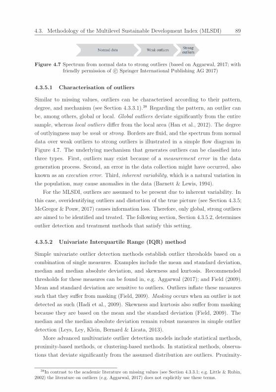
4.3. Methodology of the Multilevel Sustainable Development Index (MLSDI) 89
Figure 4.7 Spectrum from normal data to strong outliers (based on Aggarwal, 2017; withfriendly permission of c© Springer International Publishing AG 2017)
4.3.5.1 Characterisation of outliers
Similar to missing values, outliers can be characterised according to their pattern,
degree, and mechanism (see Section 4.3.3.1).38 Regarding the pattern, an outlier can
be, among others, global or local. Global outliers deviate significantly from the entire
sample, whereas local outliers differ from the local area (Han et al., 2012). The degree
of outlyingness may be weak or strong. Borders are fluid, and the spectrum from normal
data over weak outliers to strong outliers is illustrated in a simple flow diagram in
Figure 4.7. The underlying mechanism that generates outliers can be classified into
three types. First, outliers may exist because of a measurement error in the data
generation process. Second, an error in the data collection might have occurred, also
known as an execution error. Third, inherent variability, which is a natural variation in
the population, may cause anomalies in the data (Barnett & Lewis, 1994).
For the MLSDI, outliers are assumed to be present due to inherent variability. In
this case, overidentifying outliers and distortion of the true picture (see Section 4.3.5;
McGregor & Pouw, 2017) causes information loss. Therefore, only global, strong outliers
are aimed to be identified and treated. The following section, Section 4.3.5.2, determines
outlier detection and treatment methods that satisfy this setting.
4.3.5.2 Univariate Interquartile Range (IQR) method
Simple univariate outlier detection methods establish outlier thresholds based on a
combination of single measures. Examples include the mean and standard deviation,
median and median absolute deviation, and skewness and kurtosis. Recommended
thresholds for these measures can be found in, e.g. Aggarwal (2017); and Field (2009).
Mean and standard deviation are sensitive to outliers. Outliers inflate these measures
such that they suffer from masking (Field, 2009). Masking occurs when an outlier is not
detected as such (Hadi et al., 2009). Skewness and kurtosis also suffer from masking
because they are based on the mean and the standard deviation (Field, 2009). The
median and the median absolute deviation remain robust measures in simple outlier
detection (Leys, Ley, Klein, Bernard & Licata, 2013).
More advanced multivariate outlier detection models include statistical methods,
proximity-based methods, or clustering-based methods. In statistical methods, observa-
tions that deviate significantly from the assumed distribution are outliers. Proximity-
38In contrast to the academic literature on missing values (see Section 4.3.3.1; e.g. Little & Rubin,2002) the literature on outliers (e.g. Aggarwal, 2017) does not explicitly use these terms.
90 Chapter 4. Methodology
based methods detect outliers based on proximity measures from a data point to its
neighbours. Last, clustering-based methods declare data points as outliers that belong to
a small or no cluster (Han et al., 2012). Each method has advantages and disadvantages,
and details can be found in, e.g. Aggarwal (2017); and Han et al. (2012). Simulation
studies suggest preferring proximity-based over clustering-based methods (e.g. Aggarwal
& Sathe, 2015, 2017; Goldstein & Uchida, 2016), and generally, simple intuitive models
are likely to yield better results than highly complex models (Aggarwal, 2017).
For the MLSDI, outliers are detected by univariate methods because the primary
goal of outlier detection is the reduction of scale distortion (see Section 4.3.5), and
scaling is a univariate task (see Section 4.3.6.1). Two robust univariate outlier detection
methods that are based on the median and the median absolute deviation are present.
First, the Interquartile Range (IQR) method classifies an observation as outlying if it
surpasses or falls below the outlier thresholds θ. These are defined by:
⎧⎪⎨⎪⎩
θmax(y, r) = Q3(y, r) + α · q(y, r)
θmin(y, r) = Q1(y, r)− α · q(y, r)
⎫⎪⎬⎪⎭ , (4.10)
where θmax is the upper threshold, θmin represents the lower threshold, α portrays
the outlier coefficient, Q3 is the 75th percentile, Q1 depicts the 25th percentile, and q
measures the IQR. The outlier coefficient α is typically set equal to 1.5. The 75th
percentile is also called the third or upper quartile and cuts off the highest 25% of the
data. Accordingly, the 25th percentile is also referred to as the first or lower quartile
and truncates the lowest 25% of the data (Aggarwal, 2017; Han et al., 2012). Last, the
IQR q is described by:
q(y, r) = Q3(y, r)−Q1(y, r). (4.11)
The second method that is based on the median and the median absolute deviation
is suggested by Leys et al. (2013). The 75th and the 25th percentiles Q3 and Q1 of
Equation (4.10) are replaced by the median, and the IQR q is substituted by the median
absolute deviation. The outlier coefficient α is recommended to be set equal to 2.5.
Both methods are essentially the same because they are based on deviations from the
median. As the IQR method is more widely spread and used in, for example, boxplots
(see Figure 5.7b and Figure 5.8b; e.g. Han et al., 2012), the IQR method is applied in
the MLSDI, with the typical coefficient α set equal to 1.5.
After outlier detection, outlier treatment is the next step. It can be conducted in four
ways: Outliers may be removed and ignored; data may be transformed, such that outliers
do not occur; outliers may be weighted less; or the score of the outlying observation
may be changed (Field, 2009). Analogous to addressing missing values, removing
and weighting are procedures that yield invalid inferences (see Section 4.3.3; Rassler
et al., 2013). Furthermore, transformations are not recommended in index calculation.

4.3. Methodology of the Multilevel Sustainable Development Index (MLSDI) 91
First, a transformation is a form of scaling (Pollesch & Dale, 2016), and clarity may
be forfeited if it is performed in addition to scaling for indicator comparability (see
Section 4.3.6). Second, particularly non-linear transformations are harmful in index
calculation because they impact correlations (Oh & Lee, 1994), while the determination
of the key indicators’ weights is based on correlation analysis (see Section 4.3.7). In
conclusion, an outlying sustainable development key indicator yo is treated by changing
its score to the thresholds θ:
y(n, t, r) = yo(n, t, r) =
⎧⎨⎩θmax(y, r), if y(n, t, r) > θmax(y, r)
θmin(y, r), if y(n, t, r) < θmin(y, r), (4.12)
where yoε[1, Yo].
The MLSDI’s outlier detection and treatment cannot be tested because it is an
unsupervised problem setting. The true outlyingness is unknown and impossible to
learn (Aggarwal, 2017).
4.3.6 Scaling
By definition, a variety of key indicators y are reported in index calculation. These
typically feature diverse units (Pollesch & Dale, 2016), such that the required cross
indicator comparability (see Table 3.1; e.g. Pinter et al., 2018) and meaningful ag-
gregation (see Section 4.3.8; e.g. Ebert & Welsch, 2004) for methodological soundness
in terms of credibility, validity, and reliability (see Table 3.1; e.g. Cash et al., 2003;
Janouskova et al., 2018) is not guaranteed. To ensure achievement of these principles,
key indicators y are scaled. As stated in Section 4.3.4, scaling is a univariate problem
and refers to the transformation of diverse scales into one common scale (Pollesch &
Dale, 2016). The denotation “scaling” is exclusively used for the present calculation
step of unifying key indicators’ scales. Scales are time invariant but may vary over
geographical regions (see Section 4.3.5; Nardo et al., 2008; Nilsson et al., 2016).
Non-internal scaling depends on additional exogenous data (Pollesch & Dale, 2016)
and should be deployed in sustainable development indices to incorporate targets and
boundaries, enabling the assessment principle target and boundary orientedness (see
Table 3.1; Sala et al., 2015). Resulting scores from this type of scaling can then be
interpreted as distance to target (Moldan et al., 2012; Pollesch & Dale, 2016). The
scaling procedure should also minimise information loss (Zhou et al., 2006; Zhou et al.,
2010), and resulting scales should be easily understandable to effectively communicate
an index’s results, attracting a broad audience (see Table 3.1; e.g. Pinter et al., 2018).
In the following, scales are characterised in Section 4.3.6.1, and the MLSDI’s scaling
procedure is derived and described in Section 4.3.6.2.

92 Chapter 4. Methodology
4.3.6.1 Characterisation of scales
To fully understand a sustainable development index’s scaling problem, several defin-
itions are introduced. Subsequently, scales of a sustainable development index are
characterised. A scale is the dimension (e.g. temporal, spatial, or analytical) used
to measure a phenomenon. Its extent forms the overall size or magnitude, and its
resolution regards the precision (Gibson et al., 2000; Rotmans, 2002). An absolute
scale is objectively calibrated, whereas a relative scale is a transformation of the former
to picture relationships of objects to each other (Gibson et al., 2000; Turner, Dale &
Gardner, 1989). A scale’s type can be nominal, ordinal, interval, or ratio. A nominal
scale assigns labels; an ordinal scale results from rank ordering (Pollesch & Dale, 2016;
Stevens, 1946); an interval scale preserves constant distances between values, and zero
does not indicate absence of a variable; and last, a ratio scale is characterised by a
natural fixed origin, with a vanished variable at zero. The type of scale determines the
form of a variable’s comparability. A nominal variable’s equality may be ascertained,
an ordinal variable’s ordinal position may be determined, an interval variable’s absolute
differences may be evaluated, and a relative distance of a ratio variable may be assessed
(Ebert & Welsch, 2004; Pollesch & Dale, 2016; Stevens, 1946).
A sustainable development index’s scales correspond to the conceptual framework’s
dimensions (see Figure 2.11). Table 4.3 reports the technical dimension, extent, resol-
ution, hierarchy, relation, and type of each conceptual dimension that is captured in
the MLSDI. The temporal horizon contains yearly reported time periods t and is an
absolute interval scale (Gibson et al., 2000; Stevens, 1946). The contentual domain is an
analytical scale (Gibson et al., 2000) and is composed of key indicators y with diverse
units on relative ratio scales (see Section 4.3.4; Pollesch & Dale, 2015). Geographical
regions r are recorded in countries on an absolute nominal scale.39 The change agent
group business is a quantitative dimension (Gibson et al., 2000) with economic objects
n on an absolute nominal scale. Hierarchical ordering of economic objects n occurs
when incorporating the multilevel perspective (see Section 2.3.1; Rotmans et al., 2001)
and the dimension aggregational size. The aggregational size is a functional dimension
(Rotmans, 2002), which is organised in an inclusive hierarchy (see Section 4.3.1; Gib-
son et al., 2000) and features a trivariate resolution (micro, meso, and macro). The
decisional tier is also classified as a functional dimension, with the trivariate options
operational, strategic, and normative (see Section 2.3.2; e.g. Baumgartner, 2014). All
scales except the functional scales are captured in the MLSDI’s data structure (see
Figure 4.5). The aggregational size is included in the economic objects n, and the
decisional tier is addressed before and after the calculation in conceptualisation and
decision making.
39Any other resolution for time periods t and geographical regions r is possible but may be limitedby data availability.
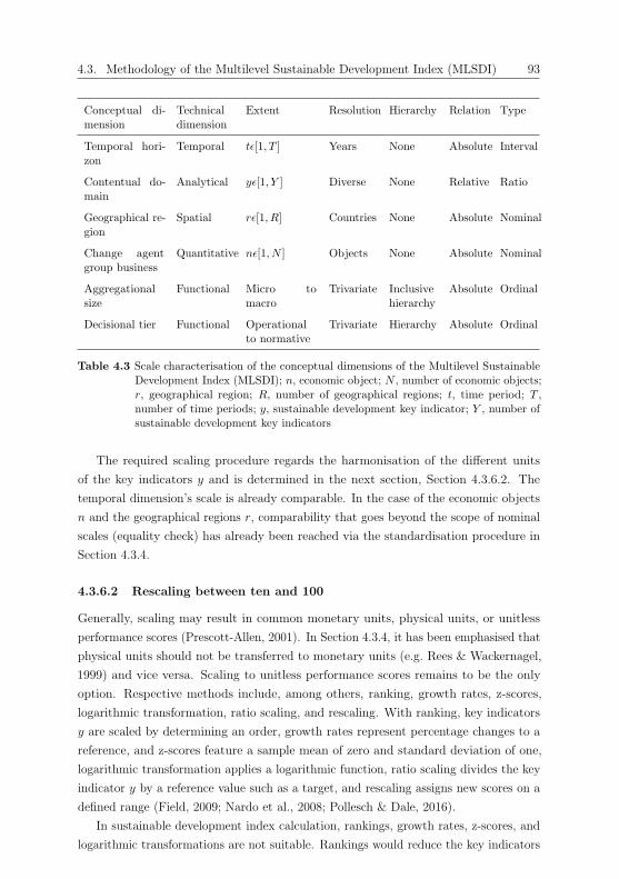
4.3. Methodology of the Multilevel Sustainable Development Index (MLSDI) 93
Conceptual di-mension
Technicaldimension
Extent Resolution Hierarchy Relation Type
Temporal hori-zon
Temporal tε[1, T ] Years None Absolute Interval
Contentual do-main
Analytical yε[1, Y ] Diverse None Relative Ratio
Geographical re-gion
Spatial rε[1, R] Countries None Absolute Nominal
Change agentgroup business
Quantitative nε[1, N ] Objects None Absolute Nominal
Aggregationalsize
Functional Micro tomacro
Trivariate Inclusivehierarchy
Absolute Ordinal
Decisional tier Functional Operationalto normative
Trivariate Hierarchy Absolute Ordinal
Table 4.3 Scale characterisation of the conceptual dimensions of the Multilevel SustainableDevelopment Index (MLSDI); n, economic object; N , number of economic objects;r, geographical region; R, number of geographical regions; t, time period; T ,number of time periods; y, sustainable development key indicator; Y , number ofsustainable development key indicators
The required scaling procedure regards the harmonisation of the different units
of the key indicators y and is determined in the next section, Section 4.3.6.2. The
temporal dimension’s scale is already comparable. In the case of the economic objects
n and the geographical regions r, comparability that goes beyond the scope of nominal
scales (equality check) has already been reached via the standardisation procedure in
Section 4.3.4.
4.3.6.2 Rescaling between ten and 100
Generally, scaling may result in common monetary units, physical units, or unitless
performance scores (Prescott-Allen, 2001). In Section 4.3.4, it has been emphasised that
physical units should not be transferred to monetary units (e.g. Rees & Wackernagel,
1999) and vice versa. Scaling to unitless performance scores remains to be the only
option. Respective methods include, among others, ranking, growth rates, z-scores,
logarithmic transformation, ratio scaling, and rescaling. With ranking, key indicators
y are scaled by determining an order, growth rates represent percentage changes to a
reference, and z-scores feature a sample mean of zero and standard deviation of one,
logarithmic transformation applies a logarithmic function, ratio scaling divides the key
indicator y by a reference value such as a target, and rescaling assigns new scores on a
defined range (Field, 2009; Nardo et al., 2008; Pollesch & Dale, 2016).
In sustainable development index calculation, rankings, growth rates, z-scores, and
logarithmic transformations are not suitable. Rankings would reduce the key indicators

94 Chapter 4. Methodology
y to ordinal scales, leading to information loss. Growth rates would entail information
loss of the original scores (Nardo et al., 2008), and growth rates are not able to
include targets and boundaries.40 Z-scores are difficult to interpret because a z-score
indicates the distance to the mean measured in standard deviations. Furthermore,
z-scores are defined on positive and negative value ranges, limiting the possibilities of
aggregation (see Section 4.3.8). However, z-scores are required for multivariate statistical
weighting techniques (see Section 4.3.7.2 and Section 4.3.7.3). Last, because logarithmic
transformations are non-linear, they are harmful in index calculation and should not
be applied. Non-linear transformations affect correlations (see Section 4.3.5.2; Oh &
Lee, 1994), which are investigated in the weighting process (see Section 4.3.7). Nardo
et al.’s (2008) statement that arithmetic aggregation of logarithmically transformed
indicators is equivalent to geometric aggregation of non-transformed indicators only
holds true if weights are not derived by statistical procedures. This in turn is not the
ideal approach (see Section 4.3.7). Ratio scaling is a candidate for the key indicators’
scaling procedure because it does not result in information loss nor in negative values.
Moreover, targets and boundaries can be included. However, ratio scaling affects key
indicators y differently depending on their effective direction ξ. Rescaling in combination
with target setting stands out as a scaling method (Pollesch & Dale, 2016).41 Targets
and boundaries can be included, and mathematical discrepancies between key indicators
y of different effective directions ξ are not present (Pollesch & Dale, 2016). Last,
resulting scores are straightforward to interpret: The score depicts the performance of
an economic object n in time period t in geographical region r relative to the minimum
of the rescaling range δmin and the maximum of the rescaling range δmax. This clear
interpretation benefits the assessment principle effective communication (see Table 3.1;
e.g. Pinter et al., 2018).
For the MLSDI, key indicators y are rescaled on an identical range from ten to 100.
A minimum of zero is avoided because the subsequent geometric aggregation would lead
to an overall index score of zero (see Equation (4.25); Saisana & Philippas, 2012). For
key indicators y with a positive effective direction ξ+, a rescaled score of ten represents
the minimum of a sustainable development key indicator in the sample ymin, and a
rescaled score of 100 depicts the maximum of a sustainable development key indicator
in the sample ymax. For key indicators y with a negative effective direction ξ−, minima
ymin and maxima ymax are reverted. Moreover, a score of ten indicates a boundary,
whereas a score of 100 denotes a target. If an economic object n exceeds a target, the
rescaled score will be higher than 100. However, targets and boundaries have not been
finalised at corporate nor at national levels yet (see Section 6.3; e.g. O’Neill et al., 2018;
40In this context, growth rates would only refer to ratio indicators yr. Growth indicators yg (seeSection 4.3.4) would not require a further scaling.
41Pollesch and Dale (2016) refer to rescaling with target setting as “target normalisation”. Thisterm is not adopted because it does not indicate the underlying scaling method and could be mistakenfor ratio scaling with target setting.

4.3. Methodology of the Multilevel Sustainable Development Index (MLSDI) 95
Whiteman et al., 2013). Therefore, the rescaling range is merely determined by internal
data. For positively affecting key indicators y, a rescaled score of 100 represents the
sample maximum of the respective key indicator ymax. For negatively affecting key
indicators y, a rescaled score of 100 represents the sample minimum of the respective
key indicator ymin. Scores that exceed 100 are not possible with internal scaling. To
realise the above described rescaling, a rescaled sustainable development key indicator
ys is computed by the following formula (Bravo, 2014; Krajnc & Glavic, 2005; Saisana
& Philippas, 2012):
ys(n, t, r) =
⎧⎨⎩(δmax − δmin)
y(n,t,r)−ymin(r)ymax(r)−ymin(r)
+ δmin, if ξ = ξ+
(δmax − δmin)ymax(r)−y(n,t,r)ymax(r)−ymin(r)
+ δmin, if ξ = ξ−, (4.13)
where ysε[1, Ys] and Ys = Y . A rescaled key indicator ys may be a rescaled sustainable
development ratio indicator yrsε[1, Yrs] or a rescaled sustainable development growth
indicator ygsε[1, Ygs]. Because rescaling relies on the extremes (i.e. ymax and ymin), it is
highly sensitive to outliers (Nardo et al., 2008). Hence, outliers have been detected and
treated in the previous calculation step (see Section 4.3.5.2).
The rescaled scores are interpreted as follows (Prescott-Allen, 2001):
• 10 ≤ ys < 20: bad performance (unacceptable),
• 20 ≤ ys < 40: poor performance (undesirable),
• 40 ≤ ys < 60: medium performance,
• 60 ≤ ys < 80: fair performance (acceptable),
• 80 ≤ ys ≤ 100: good performance (desirable).
The set of rescaled sustainable development indicators c4s is formally described by:
c4s = c4s(n, ys, t, r). (4.14)
The rescaled key indicators ys are weighted in the following section, Section 4.3.7.
4.3.7 Weighting
Weighting in index calculation refers to the process of assigning coefficients to the
index’s underlying variables in order to increase or decrease a variable’s importance
on the composite measure (Greco et al., 2019; Nardo et al., 2008). In sustainable
development index calculation, weighting leads to compliance of the principles synergies
and trade-offs as well as relevance: Weighting integrates themes, addresses relation-
ships, determines interconnection of goals, and assesses their unequal contributions
to sustainable development (see Table 3.1; e.g. Costanza, Fioramonti & Kubiszewski,
2016; Janouskova et al., 2018). Eventually, weighting closes the knowledge gap (see

96 Chapter 4. Methodology
Section 2.3.3; e.g. Weitz et al., 2018). Moreover, weighting ideally captures the relative
benefit or harmfulness to society (T. Hahn & Figge, 2011) and should be objective (see
Table 3.1; Sala et al., 2015).
In the MLSDI’s weighting procedure, all contentual domains are addressed simul-
taneously in a multivariate setting because sustainable development is one integrated
crisis and not three separate crises (see Section 2.1; WSSD, 2002). However, to account
for the unbalanced number of key indicators y within the three contentual domains (see
Section 5.3.1), the initially estimated coefficients are adjusted to sum up to one in each
domain. An adjusted coefficient is a weight, denoting a key indicator’s importance within
a domain. An importance factor is a modified weight that signals a key indicator’s
influence on the overall index (Becker et al., 2017). The modification is accomplished
by the rule of three: Weights are related to the number of indicators within a domain,
and importance factors are related to the total number of indicators included in the
MLSDI. Consistent with outlier detection and scales, weights are time invariant but
may vary over geographical regions r (see Section 4.3.5 and Section 4.3.6; Nardo et al.,
2008; Nilsson et al., 2016).
In the following section, Section 4.3.7.1, an overview on weighting methods is
given to determine the MLSDI’s approach. The applied methods are introduced in
Section 4.3.7.2 to Section 4.3.7.4. Statistical tests are performed in Section 4.3.7.5.
4.3.7.1 Overview of weighting methods
Weighting methods in sustainable development index construction are controversially
discussed because a range of possible pathways to sustainability exists (see Section 2.2.4;
Leach et al., 2013). These possibilities are coupled with uncertainties in, for example,
the environmental domain (see Section 2.2.1; Steffen et al., 2015). Weights of the
environmental domain can only be determined properly if the natural scientific rela-
tionship is known (see Section 6.3; Ebert & Welsch, 2004). Established targets and
boundaries are irrelevant for the weighting method because they are limits expressed
in the scales (see Section 4.3.6.2). The possible pathways and uncertainties lead to
three different approaches on weighting: expert surveys, equal weighting, and statistical
weighting. Expert surveys and inclusion of subjective opinion can be advantageous be-
cause, for example, experts are a key source of information in corporate decision making
(Escrig-Olmedo, Munoz-Torres, Fernandez-Izquierdo & Rivera-Lirio, 2017). However,
subjective methods are severely criticised because subjectivity leads to volatile results,
disagreements, and a lack of science (Giannetti, Bonilla, Silva & Villas Boas de Almeida,
2009; Rogge, 2012). Mixed methods such as multicriteria decision-making methods
(e.g. Boggia & Cortina, 2010; Triantaphyllou, 2000) reduce the amount of subjectivity
by providing “objective mathematics to process subjective and personal preferences”
(Saaty, 2001). One example of such a method is the analytical hierarchy process.
4.3. Methodology of the Multilevel Sustainable Development Index (MLSDI) 97
Weights are determined by decomposing the problem into a system of hierarchies and
comparing the decomposed elements in a pairwise manner (Saaty, 1980; Triantaphyllou,
2000). Despite being diminished, subjectivity remains a critical issue (Zhou et al.,
2006) as decision makers might be tempted to take advantage of their mediating power
(see Section 3.2; Jesinghaus, 2018). Second, e.g. Schmidt-Traub et al. (2017b) argue
equal weighting should be applied because a consensus on weights in expert surveys
could not be established, and equal weights would reflect a policy maker’s commitment
of equal goal priority. Further arguments for equal weighting include simplicity of
construction, a lack of theoretical structure to justify other weighting schemes, and
inadequate statistical knowledge (Decancq & Lugo, 2013; Greco et al., 2019; Nardo
et al., 2008). Top-down equal weighting is an enhanced version of equal weighting
because variables are first equally weighted into categories, then categories are equally
weighted into domains, and last, domains are equally weighted into an overall index
(e.g. Schmidt-Traub et al., 2017b; Zuo et al., 2017). Nilsson et al. (2016) warn to ignore
overlaps of targets and goals: Double counting would occur, resulting in an implicit
higher weighting of equally weighted correlated variables (Greco et al., 2019; Nardo
et al., 2008). Rogge (2012) also concludes that the simplicity of equal weighting “is
often thoroughly misleading”. In conclusion, equal weighting is “convenient but [...]
universally considered to be wrong” (Chowdhury & Squire, 2006; Decancq & Lugo, 2013;
Greco et al., 2019). To tackle synergies and trade-offs as well as relevance, statistical
methods must be applied until the natural scientific relationships are known (see above;
Ebert & Welsch, 2004) because statistical weighting is least biased and least subjective
(Greco et al., 2019; Mayer, 2008; Zhou, Ang & Poh, 2007).
Statistical weighting in index calculation essentially regards data reduction (Mayer,
2008). The sustainable development elements (i.e. the rescaled key indicators ys) are
cleaned with respect to correlations and mutually included information. Multivariate
statistical techniques for dimensionality reduction include a variety of methods, and an
overview can be found in, e.g. Meng et al. (2016). In the field of sustainable development
assessment, data envelopment analysis, factor analysis, and PCA are conducted (e.g.
Bolcarova & Kolosta, 2015; Shaker, 2018; Tseng et al., 2018; B. Zhang et al., 2008;
Zhou et al., 2007). Data envelopment analysis is not suitable as a weighting method for
a sustainable development index because it is a technique for measuring efficiencies of
decision-making objects, not being concerned with data reduction (Charnes, Cooper &
Rhodes, 1978; Ramanathan, 2003; Rogge, 2012). Moreover, efficiencies are obtained
by dividing weighted sums of data outputs by weighted sums of data inputs. Weights
in turn are determined by an optimisation function defined by the modeller (Greco
et al., 2019). This procedure entails three issues. First, weights maximise the composite
indicator (Ramanathan, 2003), while sustainable development index construction is
not an optimisation problem. Instead, the index is designed to quantify unsupervised
sustainable development performances (see Chapter 3 and Chapter 4; e.g. Bell &

98 Chapter 4. Methodology
Morse, 2008). Data envelopment analysis overemphasises well-performing elements,
such that economic objects n may appear as brilliant performers, while they are not
(Rogge, 2012). Second, the target function involves a modeller’s subjectivity, and third,
aggregation by weighted sums does not minimise substitutability as required along with
weak sustainability (see Section 2.2.4 and Section 4.3.8). Factor analysis and PCA are
dimensionality reduction techniques and generally suitable for weighting. They are
closely related to each other but differ in the direction of analysis. Factor analysis is
a top-down approach that aims to describe a number of latent factors with a smaller
number of observed variables. A model is fitted, and the solution to it is non-unique
(Haerdle & Simar, 2012). PCA functions vice versa: PCA is a bottom-up method
that reduces observed variables into a smaller number of latent components. Because
sustainable development index calculation is an unsupervised modelling task, it is a
bottom-up problem setting in which the latent index is driven by the behaviour of
the observed variables (Mayer, 2008). Consequently, PCA instead of factor analysis
is suitable for weighting. Furthermore, PCA yields one unique solution, such that
subjective interpretations are absent (Haerdle & Simar, 2012). However, factor analysis
is a useful tool in problem settings such as studied by Tseng et al. (2018). An explanatory
factor analysis is applied to derive latent constructs by underlying, observed attributes
of corporate sustainability such as stakeholder management and corporate culture.
The next section, Section 4.3.7.2, describes the PCA as the first method to derive
a weight of a sustainable development key indicator ω and an importance factor of a
sustainable development key indicator ψ. Two further methods follow in Section 4.3.7.3
and Section 4.3.7.4.
4.3.7.2 Multivariate statistical analysis: Principal Component Analysis
(PCA)
PCA (Pearson, 1901) is a linear, static technique to reduce a data set’s dimensionality
by only incorporating data that are responsible for a certain variation (Haerdle & Simar,
2012; G. James et al., 2013; Jolliffe, 2002). This technique can be used for determining
key indicators’ weights ω because rescaled key indicators ys that are responsible for
more variation in the data set contain more information and should thus receive a higher
weight. Because PCA focuses on variances (G. James et al., 2013; Jolliffe, 2002), data
must be free of outliers and z-score scaled (see Section 4.3.5.2 and Section 4.3.6.2; Field,
2009). Otherwise, weights of high variance variables would be overestimated (G. James
et al., 2013). PCA does not impose a distributional assumption (Jolliffe, 2002), but as
linear correlations are investigated, it is assumed that variables are linearly related.
To achieve the dimensionality reduction, data are transformed to a number of latent,
uncorrelated Principal Components (PCs), which are sorted in a descending order
according to their variation along with the original data set (G. James et al., 2013;

4.3. Methodology of the Multilevel Sustainable Development Index (MLSDI) 99
Jolliffe, 2002). A system of linear equations is set up and solved subject to several
constraints. The linear equations contain original variables and associated coefficients,
also referred to as loadings. The first PC is found by maximising the PC’s variance
subject to the loadings having a unit length of one. This is obtained by equalising the
sum of squared elements of the vector of loadings to one. The second PC is derived by
maximising the variance and appending the constraint of being orthogonal to the first
PC; the product of the first and the second PCs’ loadings is equalised to zero. The
following PCs are found in a similar fashion. After solving the system for each equation,
each PC’s loading and eigenvalue are specified (Jolliffe, 2002). Definitions of eigenvalues
are typically complex, mathematical definitions (Field, 2009) and can be found in, e.g.
Haerdle and Simar (2012). In PCA, eigenvalues refer to the variance-covariance matrix
and reveal the evenness of distribution of variances throughout the data set (Field, 2009).
Loadings are stored in a matrix with variables in the rows and PCs in the columns
(Jolliffe, 2002). Squaring each element of this matrix yields the substantive importance
of a variable to a PC (Field, 2009). To receive the weights, this matrix is multiplied
with a vector of variances of the PCs. However, not all PCs are included, but only a
few are chosen that adequately account for a certain variation in the data set. Rules for
inclusion involve thresholds on eigenvalues and the explained cumulative variance. These
thresholds are critically discussed in the literature. Kaiser (1960) suggests including
PCs with eigenvalues larger than one as these explain at least one variable. Jolliffe
(2002) argues that Kaiser’s (1960) criterion is too strict and recommends a threshold
of 0.7. There is evidence that Kaiser’s (1960) criterion is accurate if the chosen PCs
explain a cumulative variance greater or equal than 70% with a sample size smaller
than 30 or 60% with a sample size greater than 250 (Field, 2009).
For the MLSDI, the sample size equals 62 (see Section 5.1), and thus, PCs with
eigenvalues larger than one or to reach a cumulative variance of 70% are included.
The PCA is performed (CRAN, 2019) for each time period t, and a weight of a
sustainable development key indicator derived by the PCA ωPCA is obtained by applying
the arithmetic mean over the time periods t:
ωPCA(ys, r) =1
T
T∑t=1
ωPCAt (ys, t, r), (4.15)
where ωPCAt represents a weight of a sustainable development key indicator derived
by the PCA in a time period t. The corresponding importance factor of a sustainable
development key indicator derived by the PCA ψPCA is formally represented by:
ψPCA = ψPCA(ys, r). (4.16)
A PC is the weighted sum of the loadings and z-score scaled key indicators yz, where

100 Chapter 4. Methodology
yzε[1, Yz] and Yz = Y . It corresponds to a sustainable development key component
p, and its set – the set of sustainable development key components c3 – is formally
represented by:
c3 = c3(n, p, t, r), (4.17)
where pε[1, P ]. However, as the weighted sum is not deployed for aggregation (see
Section 4.3.8), key components p and their set c3 are obsolete.
Disadvantages of the PCA are incorrect assessment of the temporal dimension and
limitation to linearity (see above). In the following section, Section 4.3.7.3, the PCA is
extended to the Partial Triadic Analysis (PTA) to overcome the first shortcoming of
the incorrect temporal assessment.
4.3.7.3 Multivariate statistical analysis: Partial Triadic Analysis (PTA)
The PTA expands the PCA by incorporating time. Three-dimensional panel data
are interpreted as a sequence of two-dimensional tables.42 In doing so, a multivariate
time series structure is captured in three steps. The first step is called interstructure
and aims to derive the importance of each time period. A matrix of scalar products
between two-dimensional tables is computed to derive temporal weights. In a second
step, the weighted sum of the original time series of tables is computed, yielding the
so-called compromise matrix. This matrix captures the common structure of the two-
dimensional tables. As a last step, rows and columns of all original tables of the time
series are projected onto a PCA of the compromise. Thus, this step is called trajectory.
The trajectories summarise the variability of the time series around the compromise
(Gallego-Alvarez, Galindo-Villardon & Rodrıguez-Rosa, 2015; Thioulouse et al., 2004).
The application utilised in the MLSDI is based on Dray, Dufour and Thioulouse
(2018). A weight of a time period derived by the PTA ΩPTA is formally denoted by:
ΩPTA = ΩPTA(t, r). (4.18)
A weight of a sustainable development key indicator derived by the PTA ωPTA is
determined similarly to the PCA (see Section 4.3.7.2), but the temporal dimension is
implicitly accounted for (see above), such that the arithmetic mean is not required:
ωPTA = ωPTA(ys, r). (4.19)
The corresponding importance factor of a sustainable development key indicator
42Several authors controversially discuss the originality and mathematical details of this approach(e.g. Kroonenberg, 1983; Thioulouse, Simier & Chessel, 2004). According to the research of this work,first versions of temporal extensions date back to Tucker (1964), who extended factor analysis tothree-dimensional matrices. Levin (1965); and Tucker (1966) followed this approach and referred to itas “three-mode factor analysis”. Kroonenberg (1983) applied the idea to PCA and named it “PartialTriadic Analysis (PTA)”. Thioulouse and Chessel (1987) first applied it to ecology.
4.3. Methodology of the Multilevel Sustainable Development Index (MLSDI) 101
derived by the PTA ψPTA is represented by:
ψPTA = ψPTA(ys, r). (4.20)
Discussion on the number of PCs to retain could not be identified in the literature.
Transferring Kaiser’s (1960) criterion to the PTA and its implicit inclusion of time,
PCs with eigenvalues exceeding the number of time periods T are retained. Given
the cumulative variance’s relative character, its threshold value remains at 70%. Key
components p would be determined analogously to their derivation in the PCA but are
also redundant (see Section 4.3.7.2).
The following section, Section 4.3.7.4, deals with the Maximum Relevance Minimum
Redundancy Backward (MRMRB) algorithm. It is an information-theoretic application
that overcomes the shortcoming of the PCA and the PTA of being limited to linearity
(see Section 4.3.7.2). Hereafter, the term “PC family” is used when referring to both
PCA and PTA. Their weights and importance factors are summarised in the symbols
ωPC and ψPC , respectively.
4.3.7.4 Information theory: Maximum Relevance Minimum Redundancy
Backward (MRMRB) algorithm
Information theory has its origins in communication theory (Shannon, 1948) but relates
to many disciplines nowadays. Of interest for this work are its relations to statistics
and computer science (Cover & Thomas, 1991). How can key indicators’ weights ω be
derived by statistical approaches of information theory, and what are efficient algorithms
in application? Motivation for information-theoretic applications are non-linearity as
well as its known efficiency and effectiveness (P. E. Meyer, 2008; P. E. Meyer, Lafitte &
Bontempi, 2008; Peng, Long & Ding, 2005; Yu & Liu, 2004). Similar to the PC family,
information theory is a bottom-up approach, in which the underlying variables drive
the index’s behaviour (see Section 4.3.7.1; Mayer, 2008).
Information-theoretic index construction may be based on the Fisher information
or entropy. Fisher information measures the amount of information that a variable
contains about a parameter and is defined in the context of a family of parametric
distributions. Similar to the Fisher information is entropy, which also measures the
amount of information a variable contains. It is a function of an underlying process’s
probability distribution and “is a measure of the average uncertainty in the random
variable”. In contrast to the Fisher information, entropy is non-parametric and defined
for all distributions (Cover & Thomas, 1991). Because an index is based on a variety
of variables that originate in diverse distributions, entropy is the preferred measure.
Mutual information is closely related to entropy and is the reduction of uncertainty in a
random variable due to another random variable. It measures the dependency between
two random variables but can be extended to be multivariate (Cover & Thomas, 1991).

102 Chapter 4. Methodology
Moreover, it is also referred to as total correlation and is a natural measure of relevance
(Jakulin & Bratko, 2004; P. E. Meyer, 2008; Watanabe, 1960). A variable is relevant
if it reduces uncertainty (Kojadinovic, 2005) and if its removal alters the overall or a
subset’s conditional probability distribution (Kohavi & John, 1997; P. E. Meyer, 2008).
In contrast, a variable is redundant if and only if it is not relevant (Yu & Liu, 2004).
To yield inference about the variables’ relationships, multivariate data are understood
as a network, and three steps are carried out. First, data are discretised, second, a
matrix containing mutual information is calculated, and third, an inference algorithm
is performed. Discretisation is the partitioning of an interval into subintervals. It
suffers from information loss because differentiation between values of one interval is
not possible (Schafer & Strimmer, 2005; Yang & Webb, 2009). Nonetheless, estimators
are constructed for discrete variables (P. E. Meyer, 2008) because simulation studies
provide evidence that discretisation yields better results than basing the analysis on
distributional assumptions (Dougherty, Kohavi & Sahami, 1995; Yang & Webb, 2009).
Several algorithms were developed to assess gene networks in the field of bioinformat-
ics (e.g. P. E. Meyer et al., 2008). These types of algorithms are of interest in sustainable
development index calculation because the individual sustainable development elements
also represent a network of mutually correlated nodes that go beyond linear correlations.
In this work, the MRMRB algorithm is deployed (P. E. Meyer et al., 2008, 2019)
because experiments deliver evidence of superior performance relative to several other
algorithms (Bourdakou, Athanasiadis & Spyrou, 2016; P. E. Meyer, Marbach, Roy &
Kellis, 2010). The MRMRB algorithm first determines the difference of mutual informa-
tion between two random variables (i.e. relevance) and the average mutual information
along the selected variables (i.e. redundancy). Subsequently, the algorithm ranks these
differences, with direct interactions being ranked before indirect interactions. As a third
step, backward elimination is performed: Variables with the lowest mutual information
are first eliminated from the network (P. E. Meyer et al., 2010). With the MRMRB
algorithm, four estimators can be implemented: empirical estimator, Miller-Madow cor-
rected estimator, Shrink entropy estimator, and Schurmann-Grassberger estimator (P. E.
Meyer et al., 2008). In calculating the MLSDI, the Miller-Madow corrected estimator is
chosen as it corrects the asymptotic bias of the empirical estimator. The Shrink entropy
estimator is less general and only suitable for small sample sizes (P. E. Meyer et al.,
2008; Schafer & Strimmer, 2005). The Schurmann-Grassberger estimator is parametric
and makes distributional assumptions (P. E. Meyer et al., 2008). Key indicators y
are discretised by equal frequency discretisation. In this discretisation method, the
partitioned interval may be of different sizes, but the frequency of occurrence within an
interval is identical in each interval (P. E. Meyer, 2008; Yang & Webb, 2009). Especially
when combined with the Miller-Madow corrected estimator, this discretisation method
is more efficient than methods such as equal width (P. E. Meyer, 2008; Yang & Webb,
2003). The number of intervals controls the variance-bias trade-off in estimation: Too
4.3. Methodology of the Multilevel Sustainable Development Index (MLSDI) 103
many intervals result in too few data points and an increased variance, whereas too few
intervals lead to information loss and an increased bias (see above; Cover & Thomas,
1991; P. E. Meyer, 2008; Yang & Webb, 2009). Recommendation by P. E. Meyer et al.
(2008); and Yang and Webb (2003) on the bin size of the interval is followed: The bin
size of equal frequency discretisation χs, which depicts the number of economic objects
N in one bin, is set equal to the square root of the sample size:
χs =√N. (4.21)
Given the square root, the number of bins of equal frequency discretisation χn is
equivalent to the bin size χs:
χn =N
χs
=N√N
=√N = χs. (4.22)
A weight of a sustainable development key indicator derived by the MRMRB algorithm
ωMRMRB is formally denoted as follows:
ωMRMRB = ωMRMRB(ys, r). (4.23)
The corresponding importance factor of a sustainable development key indicator
derived by the MRMRB ψMRMRB is formally described by:
ψMRMRB = ψMRMRB(ys, r). (4.24)
Because the MRMRB algorithm is capable of detecting higher order correlations, it
is expected to yield superior results compared to the PC family.
The next section, Section 4.3.7.5, deals with statistical tests of the PC family (see
Section 4.3.7.2 and Section 4.3.7.3). The MRMRB algorithm does not require statistical
tests because it does not make distributional assumptions (see above), and the total
correlation is simply zero in the absence of correlations (Cover & Thomas, 1991).
4.3.7.5 Statistical tests of model assumptions
The PC family is tested with the Kaiser-Meyer-Olkin (KMO) measure of sampling
adequacy (Kaiser, 1970) and Bartlett’s test of sphericity (Bartlett, 1950, 1951).43 The
KMO measure is the ratio of squared correlations between variables to the squared
partial correlation between variables. It indicates the degree of diffusion in the pattern
of correlations: A value close to zero indicates a relatively small numerator and diffusion
in the pattern of correlations, whereas a value close to one indicates a relatively large
43These tests were initially developed for factor analysis but can also be applied to PCA (Field,2009; Jolliffe, 2002).

104 Chapter 4. Methodology
numerator and a compact pattern of correlations. In the latter case, the sample is
adequate for performing the PC family (Field, 2009; Kaiser, 1970). Values of the KMO
measure and resulting factorial simplicity are interpreted as follows (Kaiser, 1974):
• KMO < 0.5: unacceptable,
• 0.5 ≤ KMO < 0.6: miserable,
• 0.6 ≤ KMO < 0.7: mediocre,
• 0.7 ≤ KMO < 0.8: middling,
• 0.8 ≤ KMO < 0.9: meritorious,
• 0.9 ≤ KMO ≤ 1.0: marvellous.
To evaluate whether the KMO measure should be based on Pearson’s coefficient or
Kendall’s tau (see Section 4.3.3.3; Field, 2009), normality of the z-score scaled key
indicators yz is tested. Similar to the key figures x, the univariate Shapiro-Wilk and
Kolmogorov-Smirnov tests are performed (see Section 4.3.3.4; e.g. CRAN, 2019). For
consistency to the PC family’s calculation procedure, tests are performed for each year
and averaged subsequently.
Bartlett’s test of sphericity examines whether there are PCs to determine. Under
the null hypothesis, the correlation matrix is proportional to the identity matrix: Group
variances are the same or similar to each other, and covariances are equal or close
to zero. In this case, variables are not correlated, and PCs do not exist. The null
hypothesis is desired to be rejected with p-values smaller than 0.05 (Field, 2009). The
same correlation coefficient (Pearson vs. Kendall) as for the KMO test is chosen.
Multicollinearity is not an issue for the PC family (Field, 2009) and thus not tested.
4.3.8 Aggregation
Aggregation theory is an area of mathematics that investigates aggregation functions
(Pollesch & Dale, 2015). An index or composite measure is an aggregate, which is
a single value that represents “an arbitrary long set of related values” (Pollesch &
Dale, 2015). An aggregation function performs the mathematical operation of mapping
diverse variables into one aggregate (Grabisch et al., 2009; Pollesch & Dale, 2015).
This mathematical operation is called aggregation. Aggregation is considered as the
major step in index construction (Zhou et al., 2010) because it moderates the degree of
substitutability (Grabisch et al., 2009). To map weak sustainability with minimised
substitutability (see Section 2.2.4), a compensatory aggregation function ought to be
applied because high input components may be offset by low input components and vice
versa. In contrast, setoffs are not possible in non-compensatory aggregation functions
(Pollesch & Dale, 2015). These hence map strong sustainability. For methodologically
sound aggregation in terms of credibility, validity, and reliability (see Table 3.1; Cash et
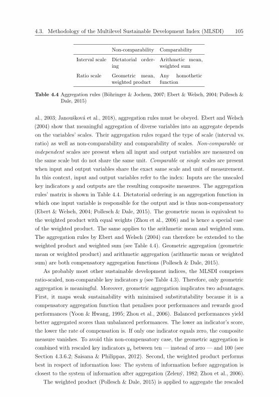
4.3. Methodology of the Multilevel Sustainable Development Index (MLSDI) 105
Non-comparability Comparability
Interval scale Dictatorial order-ing
Arithmetic mean,weighted sum
Ratio scale Geometric mean,weighted product
Any homotheticfunction
Table 4.4 Aggregation rules (Bohringer & Jochem, 2007; Ebert & Welsch, 2004; Pollesch &Dale, 2015)
al., 2003; Janouskova et al., 2018), aggregation rules must be obeyed. Ebert and Welsch
(2004) show that meaningful aggregation of diverse variables into an aggregate depends
on the variables’ scales. Their aggregation rules regard the type of scale (interval vs.
ratio) as well as non-comparability and comparability of scales. Non-comparable or
independent scales are present when all input and output variables are measured on
the same scale but do not share the same unit. Comparable or single scales are present
when input and output variables share the exact same scale and unit of measurement.
In this context, input and output variables refer to the index: Inputs are the unscaled
key indicators y and outputs are the resulting composite measures. The aggregation
rules’ matrix is shown in Table 4.4. Dictatorial ordering is an aggregation function in
which one input variable is responsible for the output and is thus non-compensatory
(Ebert & Welsch, 2004; Pollesch & Dale, 2015). The geometric mean is equivalent to
the weighted product with equal weights (Zhou et al., 2006) and is hence a special case
of the weighted product. The same applies to the arithmetic mean and weighted sum.
The aggregation rules by Ebert and Welsch (2004) can therefore be extended to the
weighted product and weighted sum (see Table 4.4). Geometric aggregation (geometric
mean or weighted product) and arithmetic aggregation (arithmetic mean or weighted
sum) are both compensatory aggregation functions (Pollesch & Dale, 2015).
As probably most other sustainable development indices, the MLSDI comprises
ratio-scaled, non-comparable key indicators y (see Table 4.3). Therefore, only geometric
aggregation is meaningful. Moreover, geometric aggregation implicates two advantages.
First, it maps weak sustainability with minimised substitutability because it is a
compensatory aggregation function that penalises poor performances and rewards good
performances (Yoon & Hwang, 1995; Zhou et al., 2006). Balanced performances yield
better aggregated scores than unbalanced performances. The lower an indicator’s score,
the lower the rate of compensation is. If only one indicator equals zero, the composite
measure vanishes. To avoid this non-compensatory case, the geometric aggregation is
combined with rescaled key indicators ys between ten — instead of zero — and 100 (see
Section 4.3.6.2; Saisana & Philippas, 2012). Second, the weighted product performs
best in respect of information loss: The system of information before aggregation is
closest to the system of information after aggregation (Zeleny, 1982; Zhou et al., 2006).
The weighted product (Pollesch & Dale, 2015) is applied to aggregate the rescaled

106 Chapter 4. Methodology
key indicators ys of a contentual domain, accounting for synergies and trade-offs (see
Table 3.1; e.g. Costanza, Fioramonti & Kubiszewski, 2016) and yielding a subindex of a
contentual domain d:
d(n, t, r) =Ys∏
ys=1
ys(n, t, r)ω(ys,r), (4.25)
where dε[1, D]. The set of sustainable development subindices c2 then reads:
c2 = c2(n, d, t, r). (4.26)
To yield the overall MLSDI c1, the geometric mean is deployed on the subindices d:
c1(n, t, r) =D∏
d=1
d(n, t, r)1D . (4.27)
Statistical weighting of the contentual domains is not feasible because methods
approximately reflect the contentual domains’ number of key indicators Y . Scores of
the four composite measures – the subindices of each contentual domains d and the
overall MLSDI c1 – are interpreted in the same fashion as the rescaled key indicators’
scores (see Section 4.3.6.2).
In the final step of the MLSDI, sensitivities are investigated. The following section,
Section 4.3.9, outlines the methodology of this investigation.
4.3.9 Sensitivity analyses
Sensitivity analysis is the study of appointing individual sources of uncertainty in the
model input to variances of the model output (Saisana, Saltelli & Tarantola, 2005; Saltelli
et al., 2008; Saltelli, Tarantola, Campolongo & Ratto, 2004). In index construction,
sensitivities of each calculation step should be analysed to ensure methodological
soundness in terms of credibility, validity, and reliability as well as robustness and
transparency (see Table 3.1; Cash et al., 2003; Janouskova et al., 2018; Pinter et al.,
2018; Saisana et al., 2005; Sala et al., 2015).
Sophisticated methods for sensitivity analyses include, for instance, elementary
effects methods, variance-based methods, factor mapping, and meta-modelling (Saltelli
et al., 2008). However, for the MLSDI, profound theoretical and methodological research
has been carried out (see Chapter 2 to Section 4.3.8), such that a simple OAT sampling
for non-unique calculation steps is sufficient. In an OAT sampling, one parameter
is varied at a time (Saltelli et al., 2008). Non-unique calculation steps that involve
alternatives are missing value imputation (see Section 4.3.3), outlier detection (see
Section 4.3.5), and weighting (see Section 4.3.7). For missing value imputation and
weighting, sensitivities of the different presented methods are investigated. Regarding
outlier detection, the outlier coefficient α is varied, and three cases are investigated:

4.4. Summary and interim conclusion 107
the outlier coefficient α equals 1.5, 3.0, and infinity. The first case is the base case (see
Section 4.3.5.2; e.g. Aggarwal, 2017) and depicts the inner fence, the second case is
laxer and constitutes the outer fence (Tukey, 1977), and the last case corresponds to a
non-treatment case (see Section 4.3.9). The latter is of importance as distortion of the
true picture is a general concern in outlier treatment (see Section 4.3.5; McGregor &
Pouw, 2017). Sensitivities are examined by economic objects’ average rank shift in the
four composite measures and changes in their performance scores (Greco et al., 2019).
4.4 Summary and interim conclusion
Thus far, a conceptual framework of sustainable development has been derived, and in
doing so, the first four related research gaps – the perspective, operational-to-normative,
knowledge, and the sustainability gaps – have been identified and partially addressed.
By including the multilevel perspective and the St. Gallen management model in
the conceptual framework, the perspective and the operational-to-normative gaps
are theoretically closed. Comprehensive and comparable measurement of sustainable
development performances by multilevel objects are inevitable for the sustainability
transition because sustainable development is a society-level concept and can only be
achieved if micro and meso objects contribute. Sustainable development assessment
principles that account for the first four related gaps assist to determine the most useful
analytical tool for a comprehensive and comparable measurement. Indicator sets that
include a composite measure stand out as such tools. Indicators are able to map all six
dimensions of the conceptual framework, including the aggregational size for multilevel
measurement, and are capable of obeying the conceptual as well as the assessment
principles. They continue closing the perspective and the operational-to-normative gaps.
Sustainable development indices address the knowledge gap by exploring synergies
and trade-offs of individual sustainable development elements. However, multilevel
sustainable development indices could not be identified in the academic literature, and
previous single level indices lack compliance of the assessment principles and exhibit
methodological shortcomings. The lack of methodological soundness constitutes the
fifth and last research gap. Hence, the MLSDI’s main contributions are multilevel
applicability and methodological strength.
To quantify meso-level corporate contributions to the macro concept sustainable
development, the MLSDI is derived in nine well-researched steps: collection of key figures,
preparation of key figures, imputation of missing values, standardisation to key indicators,
outlier detection and treatment, scaling, weighting, aggregation, and sensitivity analyses.
The data collection of key figures relies on official, open source statistics to address the
sustainability gap and ensure the assessment principle transparency. Two methods for
missing value imputation are tested: single time series imputation and multiple panel
data imputation. The key indicators are determined by aligning the meso GRI and

108 Chapter 4. Methodology
the macro SDG frameworks. Multilevel comparability is established by standardisation
to the GVA and further metrics. Macro-level GVA instead of, for example, meso-level
profits is chosen because comparable measurement of meso contributions to the macro
SDGs is aimed at. Outliers are detected and treated by the IQR method, and key
indicators are rescaled between ten and 100. Three weighting methods are examined:
the PCA, PTA, and the MRMRB algorithm. The latter is theoretically superior and
thus expected to yield more accurate results. Geometric aggregation is implemented to
project weak sustainability with minimised substitutability. Sensitivities of the four
composite measures – the three subindices and the overall MLSDI – are tested for
missing value imputation, outlier detection, and weighting. In conclusion, the MLSDI
overcomes previous indices’ methodological shortcomings in several aspects:
1. The MLSDI cleans data objectively and credibly. In contrast, only one of the
reviewed indices reduces the statistical bias of missing values objectively, and
none treats outliers credibly.
2. The MLSDI weights individual sustainable development elements by sophisticated
multivariate statistical techniques and an information-theoretic algorithm. On the
other hand, less than half of the reviewed indices investigate the interconnections
and relevance of indicators, and only one of these does so in an objective and
credible manner.
3. The MLSDI obeys mathematical aggregation rules, whereas only one third of the
reviewed indices perform objective and credible aggregation.
4. The MLSDI performs sensitivity analyses for three calculation steps. On the
contrary, only one third of the reviewed indices investigate sensitivities, and only
one of these does so for more than one calculation step.
A summary of the methodological approaches and assessment principle compliance by
each calculation step of previous sustainable development indices and the MLSDI is
displayed in Table 4.5.
In the following chapter, Chapter 5, the MLSDI is applied to a sample region.
The application crafts reliable empirical knowledge about sustainable development
performances of this region and empirically tackles the knowledge gap. By broadly
disclosing the calculation results, the sustainability gap is further approached.

4.4. Summary and interim conclusion 109
Calculation
step,
assessm
ent
principle
DJSI
ICSD
FEEM
SI
HSDI
MISD
SDGI
SDI
SSI
WI
MLSDI
1.Collection
Company
data
Company
data
IGO
data
IGO
data
UIG
Odata
Officialdata
IGO
and
fur-
ther
data
IGO
and
fur-
ther
data
Officialdata
Transp
arency
NY
YY
NY
YY
YY
2.Preparation
UN
NN
Transform
ation
tonorm
ality
NN
NN
Y
Multilev
elco
mparability
NN
NN
NN
NN
NY
Methodological
soundness
UU
UU
YU
UU
UY
3.Im
puta
tion
UN
NN
Multiple
PMea
nExpert
judge-
men
tP
Single,
multiple
Methodological
soundness
UP
NN
YN
PN
NY
4.
Sta
ndardisa-
tion
U;81
indicat-
ors
Y,
e.g.
per
production
unit;38
GRI
indicators
Y,
e.g.
per
GDP;
19
in-
dicators
Y,e.g.p.c.;4
indicators
U;31indices
Y,e.g.
p.c.;
77SDG
indic-
ators
Y,
e.g.
per
GDP;
12
in-
dicators
Y,e.g.p.c.;21
indicators
Y,
e.g.
per
GDP;
86
in-
dicators
Y,
e.g.
per
GVA;44GRI
and
SDG
indicators
†
Comprehen
siven
ess
YP
YN
UY
YY
YY
Multilev
elco
mparability
NN
NN
NN
NN
NY
Methodological
soundness
UN
YY
UY
YY
YY
Efficien
cyand
ef-
fectiven
ess
YY
YY
UY
YY
YY
5.Outlier
UN
Lower
weights
onoutliers
NN
Tru
nca
tion
of
the
bottom
below
the2.5
percentile
NThresh
olds
on
skew
ness
and
kurtosis;
non-linea
rtransform
ation
Tru
nca
tion
of
thetopabove
the90%
base-
best
IQR
method
Methodological
soundness
UP
PN
NP
NN
PY
6.Scaling
UContinuous
ratioscaling
Discrete
rescaling
Continuous
rescaling
Continuous
rescaling
Continuous
rescaling
Continuousz-
scores
Continuous
rescaling
Continuous
rescaling
Continuous
rescaling
Indicatorco
mpar-
ability
UY
YY
YY
YY
YY
Methodological
soundness
UN
NP
PY
PY
YY

110 Chapter 4. Methodology
continued
Calculation
step,
assessm
ent
principle
DJSI
ICSD
FEEM
SI
HSDI
MISD
SDGI
SDI
SSI
WI
MLSDI
Target
orien
ted-
ness
NY
YY
UY
NY
YY
Effective
commu-
nication
NN
YY
YY
NY
YY
7.W
eighting
U;
floating,
industry-
specific
weights
Analytica
lhierarchy
process
Experts’
elicitation
Equalweight-
ing
Factor
analysis
Top-down
equal
weight-
ing
PCA
Top-down
equal
weight-
ing
Arb
itrary
weighting
PCA,
PTA,
MRMRB
Synergies
and
trade-offs
UY
YN
YN
YN
UY
Methodological
soundness
NN
NN
PN
YN
NY
8.Aggregation
UArith
metic
aggregation
Choquet
integral
Geo
metricag-
gregation
Geo
metricag-
gregation
Arith
metic
aggregation
Arith
metic
aggregation
Geo
metric
ag-
gregation
Arith
metic
aggregation
Geo
metricag-
gregation
Minim
ised
substi-
tutability,
meth-
odological
sound-
ness
UN
NY
YN
NY
NY
9.
Sensitivity
analyse
sU
NW
eighting
NN
Outliers,
ag-
gregation
NW
eighting
NIm
putation,
outliers,
weighting
Methodological
soundness,
transp
arency
NN
YN
NY
NY
NY
Table
4.5
Summaryof
methodolog
ical
approaches
andassessmentprinciple
complian
ceof
previoussustainab
ledevelop
mentindices
andtheMLSDI;Y,
yes;P,partially;N,no;U,unknow
n;† ,seeSection5.3.1;DJSI,Dow
Jones
SustainabilityIndices;FEEM
SI,FEEM
SustainabilityIndex;
GDP,Gross
Dom
esticProduct;GRI,Global
Rep
ortingInitiative;GVA,Gross
ValueAdded;HSDI,Human
Sustainab
leDevelop
mentIndex;
ICSD,Com
positeSustainab
leDevelop
mentIndex;IG
O,IntergovernmentalOrgan
isation;IQ
R,Interquartile
Ran
ge;MISD,MegaIndex
ofSustainable
Development;
MRMRB,Maxim
um
Relevance
Minim
um
Redundancy
Backward
algorithm;p.c.,per
capita;PCA,Principal
ComponentAnalysis;
PTA,PartialTriadic
Analysis;
SDG,Sustainable
DevelopmentGoal;SDGI,Sustainable
DevelopmentGoalIndex;
SDI,Sustainable
DevelopmentIndex;SSI,Sustainable
SocietyIndex;W
I,WellbeingIndex
4.4. Summary and interim conclusion 111
Open Access This chapter is licensed under the terms of the Creative Commons At -tribution 4.0 International License (http://creativecommons.org/licenses/by/4.0/), which permits use, sharing, adaptation, distribution and reproduction in any medium or format, as long as you give appropriate credit to the original author(s) and the source, provide a link to the Creative Commons license and indicate if changes were made.
The images or other third party material in this chapter are included in the chapter’s Creative Commons license, unless indicated otherwise in a credit line to the mate-rial. If material is not included in the chapter’s Creative Commons license and your intended use is not permitted by statutory regulation or exceeds the permitted use, you will need to obtain permission directly from the copyright holder.
Chapter 5
Empirical findings
In this chapter, the previously developed methodology of the MLSDI (see Chapter 4) is
computed for a sample region, and the empirical findings are presented and discussed.
Thereby, the knowledge (see Section 2.3.3; e.g. Weitz et al., 2018) and the sustainability
gap (see Section 2.3.4; e.g. Hall et al., 2017) are tackled.
This chapter is structured as follows. First, the sample (except the key figures x and
the key indicators y) is introduced in Section 5.1. Hereafter, results of the sustainable
development key figures are exhibited in Section 5.2: Section 5.2.1 presents results
of the data collection and preparation process, and Section 5.2.2 fills the incomplete
sample’s data gaps. Section 5.3 deals with the multilevel key indicators y. First, they
are derived from the meso GRI and the macro SDG frameworks in Section 5.3.1, and
second, their empirical findings are analysed. To this end, summary statistics of the
unscaled growth indicators yg are investigated in Section 5.3.2, whereas an analysis
of the unscaled ratio indicators yr is refrained from, given their non-comparability.
The key indicators’ outlier detection and treatment are outlined in Section 5.3.3, and
the empirical findings of the cleaned and rescaled key indicators ys are examined in
Section 5.3.4. The main contribution to the knowledge gap’s missing understanding
of the dynamic interactions of the individual sustainable development elements makes
Section 5.4. A comparative analysis of weights ω and importance factors ψ by the three
applied weighting methods – PCA, PTA, and MRMRB algorithm – is carried out in
Section 5.4.3. Section 5.4.1 and Section 5.4.4 deal with the PC family’s statistics, and
Section 5.4.2 outlines the MRMRB algorithm’s diagnostics. Section 5.5 analyses the
four composite sustainable development measures’ summary statistics (see Section 5.5.1)
and results for the selected branches (see Section 5.5.2). Last, sensitivities of the applied
methods are tested in Section 5.6.
© The Author(s) 2021C. Lemke, Accounting and Statistical Analyses for SustainableDevelopment, Sustainable Management, Wertschöpfung undEffizienz, https://doi.org/10.1007/978-3-658-33246-4_5

114 Chapter 5. Empirical findings
5.1 Data base, objects of investigation, and time
periods
Because the MLSDI’s calculation mechanisms are driven by macro-economic objects
n (see Section 4.3.1), macro-economic data from official statistics comprise the data
base. These statistics deliver best benchmarks (Carraro et al., 2013) for methodological
soundness (see Section 3.1; e.g. Cash et al., 2003) and are open access. Therefore, they
are easily acquired (Zuo et al., 2017), and transparency is provided (see Section 3.1;
e.g. Pinter et al., 2018). As it has been anticipated in Section 4.3.2, the sample’s
geographical region r is Germany, and thus, data are collected from the following three
official institutions: Destatis, Eurostat, and the Federal Employment Agency (BA).
Destatis and Eurostat mainly cover key figures x of the environmental and the economic
domain, whereas social key figures x are primarily acquired from the BA. More
information on the collected key figures x will follow in Section 5.2.1. The time horizon
reaches from 2008 (t = 1) to 2016 (T = 9). Data before 2008 are not comparable
as they are released in a predecessor classification of the currently valid NACE Rev.
2 standard (Eurostat, 2008b). 2016 is the most recent year of major statistics by
economic objects n at the time of research (e.g. Destatis, 2018h). The macro-economic
objects n are industries or branches in NACE (see Section 4.3.2.2) that are organised
in an inclusive hierarchy (see Section 4.3.1; Gibson et al., 2000). NACE’s granularity
varies according to four levels: classes, groups, divisions, and sections. 385 classes nest
in 177 groups, 177 groups add up to 64 divisions, and 64 divisions condense into 20
sections (Eurostat, 2008b). Owing to their identifying NACE code, economic objects
n at these levels are also said to be classified at one-digit, two-digit, three-digit, or
four-digit level, respectively. For the MLSDI, computation at all levels is desired to
support the collective responsibility for sustainable development (see Section 2.1; WSSD,
2002). As many stakeholders as possible should be informed, and a broad audience
should be attracted with effective communication (see Section 3.1; e.g. Pinter et al.,
2018). However, data for groups and classes are rarely available (i.e. unit non-response
occurs), and the MLSDI’s determinative economic objects n are divisions at two-digit
level. The 64 divisions as well as their superordinate sections are listed in Table A.1 in
the Appendix A.1. The last two divisions – 97-98 Activities of households as employers;
undifferentiated goods- and services-producing activities of households for own use
and 99 Activities of extraterritorial organisations and bodies – are omitted due to
their frequent zero output (e.g. Destatis, 2018h). Therefore, the sample’s number of
economic objects N equals 62. In parts of the analysis, not all but selected economic
objects n are focused. These selected branches involve the health economy, agricultural
sector, manufacturing sector, chemical industry, car industry, service sector, Information
Technology (IT) industry, financial industry, real estate industry, and the overall German
economy. Sectors correspond to sections at one-digit level, and industries are divisions

5.1. Data base, objects of investigation, and time periods 115
Section code Division code Abbreviated denotation
n/a n/a Health economy
A-S 01-96 Overall German economy
A 01-03 Agricultural sector
C 10-33 Manufacturing sector
20 Chemical industry
29-30 Car industry
G-S 45-96 Service sector
62-63 IT industry
64 Financial industry
L 68 Real estate industry
Table 5.1 Selected branches of the sample (Eurostat, 2008b); IT, Information Technology;n/a, not applicable
at two-digit level. These abbreviated denotations and the associated NACE codes
(except for the health economy; see below) are enumerated in Table 5.1.
The health economy is a cross-sectional industry, and its definition is based on
product delimitation performed by the economic research institute WifOR and the
Federal Ministry for Economic Affairs and Energy (BMWi) (Gerlach et al., 2018). For
consistency to the MLSDI’s determinative economic objects n, the health economy is
defined at NACE two-digit level in this work. The health economy’s stakes in two-digit
divisions are attached to the Appendix A.2, Table A.2. The health economy is of
interest because it contributes most to the German GDP and labour market among
the divisions, with GVA and working population shares of 12.1% and 17.0% in 2018,
respectively (BMWi, 2019). Furthermore, corporate responsibility44 reporting in the
worldwide health economy features a considerably increasing trend: Its reporting rate
grew from 68% in 2015 to 76% in 2017 (KPMG, 2017).45 The overall German economy
and aggregated sectors (agricultural, manufacturing, and service sectors) are selected
to attract a broad audience (see above). The chemical industry is worthwhile to be
examined because of its negative impact on the environment and efforts in industry
self-regulation (e.g. Johnson, 2012; King & Lenox, 2000). Large corporations such
as BASF engage in environmental sustainable development (e.g. Saling et al., 2002;
Uhlman & Saling, 2010), voluntary initiatives such as the Responsible Care Program
(CEFIC, 2019) are found, and an industry-specific sustainable development index has
44Generally, the present work is concerned with corporate sustainability and not corporate respons-ibility (see Section 2.3.2; e.g. Bansal & Song, 2017). However, a distinction of these terms is not madein the cited reference (KPMG, 2017), and the original wording is adopted.
45Sample: 4,900 top 100 companies in terms of revenues in 49 countries, thereof corporationsallocated to healthcare.
116 Chapter 5. Empirical findings
been developed (AIChE & IfS, 2019). Similar to the health economy, the chemical
industry’s corporate responsibility reporting rate experienced a substantial increase from
75% in 2015 to 81% in 2017 (KPMG, 2017).46 In contrast, the German car industry,
which is the largest industry in the manufacturing sector in terms of GVA (share of
22.6% in 2016; Destatis, 2018h), rather attracts attention with embroilment in fraud
scandals on cars’ true Carbon Dioxide (CO2) emission factors. A timeline of the fraud
scandal can be found in, e.g. Clean Energy Wire (2019). However, the car industry
earns the fourth place in global corporate responsibility reporting, with a rate of 79% in
2017 (KPMG, 2017).47 The IT industry is examined due to digitalisation being a global
megatrend, requiring enhanced computer programming as well as data and information
services across industries and business functions (Alcacer & Cruz-Machado, 2019). Its
importance for society is also reflected by the fact that IT skills are addressed in the
SDGs (SDG 4.4.1; UN, 2018). The finance industry pursues sustainable development
by, for example, the implementation of a sustainable development index (i.e. the DJSI;
see Section 3.3.2 and Section 4.2; e.g. RobecoSAM, 2018a) or innovative sustainable
products and services (de Bettignies & Lepineux, 2009; Wiek & Weber, 2014). However,
sustainable development performances of the financial industry’s activities as a whole
might be questionable (Wiek & Weber, 2014). In terms of corporate responsibility
reporting, the financial industry decreased its rate from 75% in 2015 to 71% in 2017
(KPMG, 2017).48 Last, the real estate industry is a selected branch because housing
prices constantly rise since 2015 (Eurostat, 2019b), causing debates on inequalities and
social justice (Dustmann, Fitzenberger & Zimmermann, 2018). Moreover, it is the
biggest two-digit level industry in the service sector in terms of GVA, with a share of
15.9% in 2016 (Destatis, 2018h).
The sample does not include meso-economic objects n yet, but especially corporations
are strongly encouraged to quantify their sustainable development performances as
advised in this work. Corporations should benchmark their results to the results of
macro-economic objects n of this sample in order to derive coordinated actions for
improved sustainable development.
The next section, Section 5.2, deals with the sample’s key figures x.
5.2 Sustainable development key figures
This section presents the empirical findings of the calculation steps one to three (see
Section 4.3.1 to Section 4.3.3) and is structured accordingly. First, the MLSDI’s key
46Sample: 4,900 top 100 companies in terms of revenues in 49 countries, thereof corporationsallocated to chemicals.
47Sample: 4,900 top 100 companies in terms of revenues in 49 countries, thereof corporationsallocated to automotive.
48Sample: 4,900 top 100 companies in terms of revenues in 49 countries, thereof corporationsallocated to financial services.

5.2. Sustainable development key figures 117
figures x are collected, defined, and prepared in Section 5.2.1. Because the key figures
x are inferred from the key indicators y (see Section 4.3.1 and Section 4.3.4), derivation
of the key figures’ significance in relation to sustainable development is postponed
to Section 5.3.1. Second, results of the missing value imputation are exhibited and
discussed in Section 5.2.2.
5.2.1 Collection and preparation of sustainable development
key figures
The MLSDI’s ideal set of key indicators c4 is the intersection of the GRI and the SDG
frameworks (see Section 4.3.4 and Section 5.3.1). From this intersection, the ideal set
of key figures c5 is inferred (see Section 4.3.1). The actual sets are reduced versions
of the ideal sets because of macro-data restrictions by official statistics. Severe item
non-response entails too high uncertainties in the imputation process, and the item
is excluded from the calculation. Three different forms of severe item non-response
are present: A key figure x may be totally unavailable, only available at one-digit
level, or only available for several divisions with incomplete sections. The present
sample comprises six environmental, 16 social, and 14 economic key figures x, with the
total number of key figures X amounting to 36. The unbalanced number of available
key figures x across the contentual domains might demonstrate a focus on social and
economic issues. However, indicators of the environmental domain are less similar to
each other (e.g. the social domain contains four tax indicators; see Table 5.3) and
the main topics and impacts are covered by the relatively small number of indicators.
Table 5.2 to Table 5.4 list and characterise the MLSDI’s environmental, social, and
economic key figures x by their statistical classifications and reporting units. Data
sources are provided in the last columns of the tables.
Definitions of the key figures x are provided in the following, and if not indicated
otherwise, they are compiled by definitions of their data sources and Eurostat (2019c).
The environmental domain reports air emissions (see Table 5.2), which are the amount
of pollution of a plant or a product released into the air and include GHG emissions
according to the Kyoto protocol (UNFCCC, 1998). The value of taxes levied on
physical units that negatively impact the environment is called environmental tax and
involves energy taxes and transport taxes. Energy taxes are composed of the energy
tax, electricity tax, emission rights, fee for the Compulsory Oil Storage Association,
and the nuclear fuel tax. Transport taxes consist of the motor vehicle tax and the air
traffic tax. Hazardous waste regards the amount of hazardous substances generated by
primary producers that require records according to the European regulation of waste
(BMJV, 2019b). Primary energy consumption is the amount of energy used in the first
place, irrespective of its purpose (energy or non-energy purpose) and conversation losses
or other leakages. Waste water is used water that does not fulfil the quality criteria of

118 Chapter 5. Empirical findings
Environmental key figure x Classification Unit Data source
Air emissions CPA KilogramCO2e
Destatis, 2018f
Environmental tax NACE Euro Destatis, 2019e
Hazardous waste NACE Kilogram Destatis, 2011b, 2012b, 2013c,2014d, 2016f, 2016g, 2017d,2019d
Primary energy consumption CPA Joule Destatis, 2018e
Waste water NACE Litre Destatis, 2018g
Water use NACE Litre Destatis, 2018g
Table 5.2 List of the environmental key figures; CO2e, Carbon Dioxide Equivalents; CPA,Classification of Products by Activity; NACE, Statistical Classification of EconomicActivities in the European Community
its initial purpose. The amount of water used by end users is termed water use.
The social domain’s key figures x encompass the following (see Table 5.3). Ap-
prentices are the number of employees in vocational training. The value of tax levied
on taxable incomes of the economic objects n is referred to as the Corporate Income
Tax (CIT). The compensation of employees represents the value of remuneration by
employers to employees in return for work. It includes gross wages and salaries as well
as social insurance contributions by both employers and employees. German compulsory
social insurances involve the accident, health, nursing care, and the unemployment
insurances. The key figure employees comprises the number of people contracted to
carry out work for an employer in return for remuneration. The female labour force is
constituted by the number of economically active females and includes female employees,
self-employed, and unemployed women.49 The number of female employees with a
compensation below 450 Euro per month or a short-term contract below approximately
three months of duration are termed female marginally-employed employees. Marginal
employment is not subject to participation in the compulsory social insurances. In
contrast, the female socially-insured employees are the number of female employees
contributing to and benefiting from compulsory social insurances. The gender-unspecific
counterparts labour force, marginally-employed employees, and socially-insured employ-
ees are defined correspondingly. After defining the last type of employment in the
economic domain (see below), relations of the different employment types are established.
The allocation of employment key figures to the social as well as the economic domain
is based on the key indicators’ assignment (see Section 5.3.1.2 and Section 5.3.1.3) and
demonstrates the employment’s dual purpose: It is a source of income but goes beyond
49As unemployed people cannot be assigned to an industry, the (female) labour force is only availablefor the overall German economy. Industry-specific data are not required as the labour forces only servethe computation of the key indicators y on gender differences, further elaborated in Section 5.3.1.2.
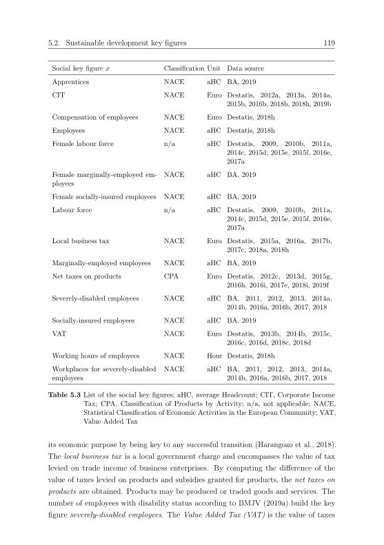
5.2. Sustainable development key figures 119
Social key figure x Classification Unit Data source
Apprentices NACE aHC BA, 2019
CIT NACE Euro Destatis, 2012a, 2013a, 2014a,2015b, 2016b, 2018b, 2018h, 2019b
Compensation of employees NACE Euro Destatis, 2018h
Employees NACE aHC Destatis, 2018h
Female labour force n/a aHC Destatis, 2009, 2010b, 2011a,2014c, 2015d, 2015e, 2015f, 2016e,2017a
Female marginally-employed em-ployees
NACE aHC BA, 2019
Female socially-insured employees NACE aHC BA, 2019
Labour force n/a aHC Destatis, 2009, 2010b, 2011a,2014c, 2015d, 2015e, 2015f, 2016e,2017a
Local business tax NACE Euro Destatis, 2015a, 2016a, 2017b,2017c, 2018a, 2018h
Marginally-employed employees NACE aHC BA, 2019
Net taxes on products CPA Euro Destatis, 2012c, 2013d, 2015g,2016h, 2016i, 2017e, 2018i, 2019f
Severely-disabled employees NACE aHC BA, 2011, 2012, 2013, 2014a,2014b, 2016a, 2016b, 2017, 2018
Socially-insured employees NACE aHC BA, 2019
VAT NACE Euro Destatis, 2013b, 2014b, 2015c,2016c, 2016d, 2018c, 2018d
Working hours of employees NACE Hour Destatis, 2018h
Workplaces for severely-disabledemployees
NACE aHC BA, 2011, 2012, 2013, 2014a,2014b, 2016a, 2016b, 2017, 2018
Table 5.3 List of the social key figures; aHC, average Headcount; CIT, Corporate IncomeTax; CPA, Classification of Products by Activity; n/a, not applicable; NACE,Statistical Classification of Economic Activities in the European Community; VAT,Value Added Tax
its economic purpose by being key to any successful transition (Harangozo et al., 2018).
The local business tax is a local government charge and encompasses the value of tax
levied on trade income of business enterprises. By computing the difference of the
value of taxes levied on products and subsidies granted for products, the net taxes on
products are obtained. Products may be produced or traded goods and services. The
number of employees with disability status according to BMJV (2019a) build the key
figure severely-disabled employees. The Value Added Tax (VAT) is the value of taxes

120 Chapter 5. Empirical findings
Economic key figure x Classification Unit Data source
Consumption of fixed capital NACE Euro Destatis, 2018h
Export CPA Euro Destatis, 2018h
Gross fixed assets NACE Euro Destatis, 2018h
Gross fixed capital formation NACE Euro Destatis, 2018h
GVA NACE Euro Destatis, 2018h
Import CPA Euro Destatis, 2018h
Imported input CPA Euro Destatis, 2012c, 2013d, 2015g,2016h, 2016i, 2017e, 2018i, 2019f
Input NACE Euro Destatis, 2018h
Internal R&D expenditures NACE Euro Eurostat, 2019a
Net fixed assets NACE Euro Destatis, 2018h
Output NACE Euro Destatis, 2018h
R&D employees NACE aHC Eurostat, 2019d
Working hours of working popu-lation
NACE Hour Destatis, 2018h
Working population NACE aHC Destatis, 2018h
Table 5.4 List of the economic key figures; aHC, average Headcount; CPA, Classificationof Products by Activity; GVA, Gross Value Added; NACE, Statistical Classific-ation of Economic Activities in the European Community; R&D, Research andDevelopment
levied on the value added of goods and services, and is computed by the difference
of total VAT and deductible VAT on inputs. The number of hours actually worked
by employees (excluding, e.g. holidays and sick days) composes the working hours of
employees. Workplaces for severely-disabled employees are the number of mandatory
workplaces for severely-disabled employees, set by an employer’s type and size.
Last, the economic domain’s key figures x (see Table 5.4) are defined. Consumption
of fixed capital is the value of impairment of fixed assets (see below). The value of goods
and services that change ownerships from residents to non-residents is termed export.
Gross fixed assets represent the reinstatement value of stock of fixed assets that are
used in production for more than one year. Fixed assets include machinery, equipment,
buildings, and other structures. The gross fixed capital formation refers to the value of
acquisitions of fixed assets, excluding fixed asset disposals, and is therefore also termed
“investment”. Definitions of GVA, output, and input can be found in Section 4.3.2.1.
The key figure import regards the value of goods and services that change ownerships
from non-residents to residents; the imported input is defined correspondingly. The value
of expenditures within a statistical unit on creative work conducted by own employees

5.2. Sustainable development key figures 121
to increase the stock and use of knowledge is reported in the internal Research and
Development (R&D) expenditures. Net fixed assets regard the current value of stock of
fixed assets, which is equivalent to gross fixed assets less the accumulated consumption
of fixed capital. The number of employees in the field of R&D depicts the key figure
R&D employees. Working hours of working population is the working population’s
equivalent of working hours of employees, where the working population represents the
number of people that perform a production activity. The relations of apprentices,
employees, labour force, marginally-employed employees, socially-insured employees,
and working population are as follows. The labour force is the broadest key figure
x as it comprises employees, self-employed, and unemployed people. The working
population is obtained by disregarding unemployed people. Self-employed people are
not further distinguished but employees are. These include apprentices, marginally-
employed employees, socially-insured employees, and further employment types such
as civil servants. However, data of these key figures x are not comparable as they are
retrieved from different data bases.
Key figures x are generally defined on a positive value range. Exceptions are the
VAT and the net taxes on products. Positive values indicate monetary outflows from
the object of investigation, and negative values denote monetary inflows to the object
of investigation.
Preparation of key figures x cover macro-level transformations from NACE to
CPA. These yield standard results and are thus not disclosed. Data sources for the
transformation include Destatis’ supply tables retrieved from the national accounts
(Destatis, 2012c, 2013d, 2015g, 2016h, 2016i, 2017e, 2018i, 2019f).
The following section, Section 5.2.2, turns the incomplete sample into a complete
one by missing value imputation.
5.2.2 Imputation of missing values
The collected sample (see Section 5.2.1) contains item non-responses and features a
general missing data pattern. Sustainable development data remain to be scarce despite
the digital era of big data that is deemed to generate richness of data and information
(Esty, 2018). 17 of 36 key figures x require missing value imputation and the average
rate of missing values λ amounts to 22.63%, with a minimum of 14.87% in 2013 and a
maximum of 32.19% in 2008. The missing data patterns of these years are illustrated
in Figure 5.1 and Figure 5.2. The x-axis contains the key figures x, while the y-axis
comprises the economic objects n. Light patches signal missing data. More than
twice as many values are missing in the service sector (λ = 28.13%) compared to
the manufacturing sector (λ = 13.29%). In Figure 5.1 and Figure 5.2, approximately
the upper half represents the manufacturing sector, and approximately the lower half
depicts the service sector (see Table A.1).

122 Chapter 5. Empirical findings
Air
emis
sion
sEn
viro
nmen
tal t
axH
azar
dous
was
tePr
imar
y en
ergy
con
sum
ptio
nW
aste
wat
erW
ater
use
App
rent
ices
CIT
Com
pens
atio
n of
em
ploy
ees
Empl
oyee
sFe
mal
e m
argi
nally
−em
ploy
ed e
mpl
oyee
sFe
mal
e so
cial
ly−i
nsur
ed e
mpl
oyee
sLo
cal b
usin
ess t
axM
argi
nally
−em
ploy
ed e
mpl
oyee
sN
et ta
xes o
n pr
oduc
tsSe
vere
ly−d
isab
led
empl
oyee
sSo
cial
ly−i
nsur
ed e
mpl
oyee
sVA
TW
orki
ng h
ours
of e
mpl
oyee
sW
orkp
lace
s for
seve
rely
−dis
able
d em
ploy
ees
Con
sum
ptio
n of
fixe
d ca
pita
lEx
port
Gro
ss fi
xed
asse
tsG
ross
fixe
d ca
pita
l for
mat
ion
GVA
Impo
rtIm
porte
d in
put
Inpu
tIn
tern
al R
&D
exp
endi
ture
sN
et fi
xed
asse
tsO
utpu
tR
&D
em
ploy
ees
Wor
king
hou
rs o
f wor
king
pop
ulat
ion
Wor
king
pop
ulat
ion
96...
...NACE code A
Observed economic objects nMissing economic objects n
Figure 5.1 Missing data pattern in the German economy in 2008; CIT, Corporate IncomeTax; GVA, Gross Value Added; NACE, Statistical Classification of EconomicActivities in the European Community; R&D, Research and Development; VAT,Value Added Tax
The first application to gain upon the data shortage is single time series imputation
(see Section 4.3.3.2). The imputation generally yields stable results, and exemplary
results of the key figure import for the selected branches are displayed in Figure 5.3. The
import’s missing data pattern is monotone in the temporal dimension and thus easily
visualised with solid lines for observed data and dashed lines for imputed data. The
Kalman smoothing and maximum likelihood estimation (see Section 4.3.3.2; e.g. Harvey,
1989) are applied on the agricultural sector and industries in the manufacturing sector
in 2008 and 2009. Industries in the service sector require modified mean imputation
as their total time series are unobserved. Because single imputation produces stable
results as expected, estimates are considered to be valid. Test results on the model

5.2. Sustainable development key figures 123
Air
emis
sion
sEn
viro
nmen
tal t
axH
azar
dous
was
tePr
imar
y en
ergy
con
sum
ptio
nW
aste
wat
erW
ater
use
App
rent
ices
CIT
Com
pens
atio
n of
em
ploy
ees
Empl
oyee
sFe
mal
e m
argi
nally
−em
ploy
ed e
mpl
oyee
sFe
mal
e so
cial
ly−i
nsur
ed e
mpl
oyee
sLo
cal b
usin
ess t
axM
argi
nally
−em
ploy
ed e
mpl
oyee
sN
et ta
xes o
n pr
oduc
tsSe
vere
ly−d
isab
led
empl
oyee
sSo
cial
ly−i
nsur
ed e
mpl
oyee
sVA
TW
orki
ng h
ours
of e
mpl
oyee
sW
orkp
lace
s for
seve
rely
−dis
able
d em
ploy
ees
Con
sum
ptio
n of
fixe
d ca
pita
lEx
port
Gro
ss fi
xed
asse
tsG
ross
fixe
d ca
pita
l for
mat
ion
GVA
Impo
rtIm
porte
d in
put
Inpu
tIn
tern
al R
&D
exp
endi
ture
sN
et fi
xed
asse
tsO
utpu
tR
&D
em
ploy
ees
Wor
king
hou
rs o
f wor
king
pop
ulat
ion
Wor
king
pop
ulat
ion
96...
...NACE code A
Observed economic objects nMissing economic objects n
Figure 5.2 Missing data pattern in the German economy in 2013; CIT, Corporate IncomeTax; GVA, Gross Value Added; NACE, Statistical Classification of EconomicActivities in the European Community; R&D, Research and Development; VAT,Value Added Tax
assumptions follow below.
With regard to Amelia II (see Section 4.3.3.3; e.g. Honaker et al., 2011), dropped,
highly correlated key figures x that are free from missing values encompass the compens-
ation of employees, employees, female marginally-employed employees, socially-insured
employees, workplaces for severely-disabled employees, consumption of fixed capital,
gross fixed assets, net fixed assets, and the output. Kendall’s tau is the used correlation
coefficient because the key figures x are non-normal (see below). The compensation of
employees and the output correlate with the GVA and the input; female marginally-
employed employees are associated with marginally-employed employees; female socially-
insured employees, socially-insured employees, and employees depend on the working
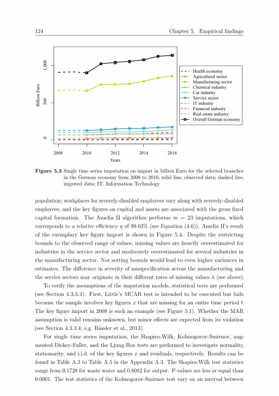
124 Chapter 5. Empirical findings
2008 2010 2012 2014 2016Years
Bill
ion
Euro
● ● ● ● ● ● ●
0
500
1,00
0
●
Health economyAgricultural sectorManufacturing sectorChemical industryCar industryService sectorIT industryFinancial industryReal estate industryOverall German economy
Figure 5.3 Single time series imputation on import in billion Euro for the selected branchesin the German economy from 2008 to 2016; solid line, observed data; dashed line,imputed data; IT, Information Technology
population; workplaces for severely-disabled employees vary along with severely-disabled
employees; and the key figures on capital and assets are associated with the gross fixed
capital formation. The Amelia II algorithm performs m = 23 imputations, which
corresponds to a relative efficiency η of 99.03% (see Equation (4.6)). Amelia II’s result
of the exemplary key figure import is shown in Figure 5.4. Despite the restricting
bounds to the observed range of values, missing values are heavily overestimated for
industries in the service sector and moderately overestimated for several industries in
the manufacturing sector. Not setting bounds would lead to even higher variances in
estimates. The difference in severity of misspecification across the manufacturing and
the service sectors may originate in their different rates of missing values λ (see above).
To verify the assumptions of the imputation models, statistical tests are performed
(see Section 4.3.3.4). First, Little’s MCAR test is intended to be executed but fails
because the sample involves key figures x that are missing for an entire time period t.
The key figure import in 2008 is such an example (see Figure 5.1). Whether the MAR
assumption is valid remains unknown, but minor effects are expected from its violation
(see Section 4.3.3.4; e.g. Rassler et al., 2013).
For single time series imputation, the Shapiro-Wilk, Kolmogorov-Smirnov, aug-
mented Dickey-Fuller, and the Ljung-Box tests are performed to investigate normality,
stationarity, and i.i.d. of the key figures x and residuals, respectively. Results can be
found in Table A.3 to Table A.5 in the Appendix A.3. The Shapiro-Wilk test statistics
range from 0.1728 for waste water and 0.8082 for output. P-values are less or equal than
0.0001. The test statistics of the Kolmogorov-Smirnov test vary on an interval between
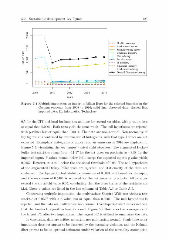
5.2. Sustainable development key figures 125
2008 2010 2012 2014 2016Years
Bill
ion
Euro
● ● ● ● ● ● ●
0
500
1,00
01,
500
2,00
0
●
Health economyAgricultural sectorManufacturing sectorChemical industryCar industryService sectorIT industryFinancial industryReal estate industryOverall German economy
Figure 5.4 Multiple imputation on import in billion Euro for the selected branches in theGerman economy from 2008 to 2016; solid line, observed data; dashed line,imputed data; IT, Information Technology
0.5 for the CIT and local business tax and one for several variables, with p-values less
or equal than 0.0001. Both tests yield the same result: The null hypotheses are rejected
with p-values less or equal than 0.0001. The data are non-normal. Non-normality of
key figures x is confirmed by examination of histograms, such that type I errors are not
expected. Exemplary histograms of import and air emissions in 2016 are displayed in
Figure 5.5, visualising the key figures’ typical right skewness. The augmented Dickey-
Fuller test statistics range from −11.17 for the net taxes on products to −3.88 for the
imported input. P-values remain below 0.01, except the imported input’s p-value yields
0.0152. However, it is still below the decisional threshold of 0.05. The null hypotheses
of the augmented Dickey-Fuller tests are rejected, and stationarity of the data are
confirmed. The Ljung-Box test statistics’ minimum of 0.0001 is obtained for the input,
and the maximum of 0.5481 is achieved for the net taxes on products. All p-values
exceed the threshold value 0.05, concluding that the error terms of the residuals are
i.i.d. These p-values are listed in the last columns of Table A.3 to Table A.5.
Concerning multiple imputation, the multivariate Shapiro-Wilk test yields a test
statistic of 0.0327 with a p-value less or equal than 0.0001. The null hypothesis is
rejected, and the data are multivariate non-normal. Overdispersed start values indicate
that the Amelia II algorithm functions well. Figure 5.6 illustrates the convergence of
the largest PC after two imputations. The largest PC is utilised to summarise the data.
In conclusion, data are neither univariate nor multivariate normal. Single time series
imputation does not appear to be distorted by the normality violation, and the Kalman
filter proves to be an optimal estimator under violation of the normality assumption
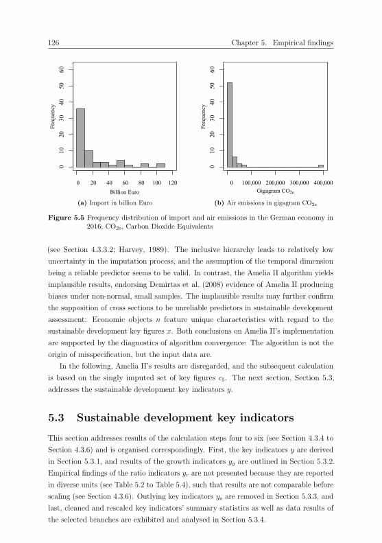
126 Chapter 5. Empirical findings
Billion Euro
Freq
uenc
y0
1020
3040
5060
0 20 40 60 80 100 120
(a) Import in billion Euro
Gigagram CO2e
Freq
uenc
y0
1020
3040
5060
0 100,000 200,000 300,000 400,000
(b) Air emissions in gigagram CO2e
Figure 5.5 Frequency distribution of import and air emissions in the German economy in2016; CO2e, Carbon Dioxide Equivalents
(see Section 4.3.3.2; Harvey, 1989). The inclusive hierarchy leads to relatively low
uncertainty in the imputation process, and the assumption of the temporal dimension
being a reliable predictor seems to be valid. In contrast, the Amelia II algorithm yields
implausible results, endorsing Demirtas et al. (2008) evidence of Amelia II producing
biases under non-normal, small samples. The implausible results may further confirm
the supposition of cross sections to be unreliable predictors in sustainable development
assessment: Economic objects n feature unique characteristics with regard to the
sustainable development key figures x. Both conclusions on Amelia II’s implementation
are supported by the diagnostics of algorithm convergence: The algorithm is not the
origin of misspecification, but the input data are.
In the following, Amelia II’s results are disregarded, and the subsequent calculation
is based on the singly imputed set of key figures c5. The next section, Section 5.3,
addresses the sustainable development key indicators y.
5.3 Sustainable development key indicators
This section addresses results of the calculation steps four to six (see Section 4.3.4 to
Section 4.3.6) and is organised correspondingly. First, the key indicators y are derived
in Section 5.3.1, and results of the growth indicators yg are outlined in Section 5.3.2.
Empirical findings of the ratio indicators yr are not presented because they are reported
in diverse units (see Table 5.2 to Table 5.4), such that results are not comparable before
scaling (see Section 4.3.6). Outlying key indicators yo are removed in Section 5.3.3, and
last, cleaned and rescaled key indicators’ summary statistics as well as data results of
the selected branches are exhibited and analysed in Section 5.3.4.
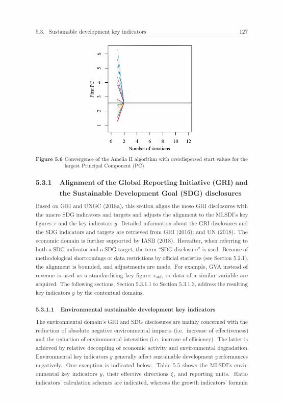
5.3. Sustainable development key indicators 127
Figure 5.6 Convergence of the Amelia II algorithm with overdispersed start values for thelargest Principal Component (PC)
5.3.1 Alignment of the Global Reporting Initiative (GRI) and
the Sustainable Development Goal (SDG) disclosures
Based on GRI and UNGC (2018a), this section aligns the meso GRI disclosures with
the macro SDG indicators and targets and adjusts the alignment to the MLSDI’s key
figures x and the key indicators y. Detailed information about the GRI disclosures and
the SDG indicators and targets are retrieved from GRI (2016); and UN (2018). The
economic domain is further supported by IASB (2018). Hereafter, when referring to
both a SDG indicator and a SDG target, the term “SDG disclosure” is used. Because of
methodological shortcomings or data restrictions by official statistics (see Section 5.2.1),
the alignment is bounded, and adjustments are made. For example, GVA instead of
revenue is used as a standardising key figure xstd, or data of a similar variable are
acquired. The following sections, Section 5.3.1.1 to Section 5.3.1.3, address the resulting
key indicators y by the contentual domains.
5.3.1.1 Environmental sustainable development key indicators
The environmental domain’s GRI and SDG disclosures are mainly concerned with the
reduction of absolute negative environmental impacts (i.e. increase of effectiveness)
and the reduction of environmental intensities (i.e. increase of efficiency). The latter is
achieved by relative decoupling of economic activity and environmental degradation.
Environmental key indicators y generally affect sustainable development performances
negatively. One exception is indicated below. Table 5.5 shows the MLSDI’s envir-
onmental key indicators y, their effective directions ξ, and reporting units. Ratio
indicators’ calculation schemes are indicated, whereas the growth indicators’ formula

128 Chapter 5. Empirical findings
Environmental key indic-ator y
Calculation scheme Effectivedirection ξ
Unit
Growth of air emissions −1 Percentage
Air emissions intensityAir emissions
GVA−1 Gram CO2e
per Euro
Growth of primary energyconsumption
−1 Percentage
Energy intensityPrimary energy consumption
GVA−1 Mega joule
per Euro
Growth of water use −1 Percentage
Water intensityWater use
GVA−1 Litre per Euro
Growth of waste water −1 Percentage
Waste water intensityWaste water
GVA−1 Litre per Euro
Growth of hazardous waste −1 Percentage
Hazardous waste intensityHazardous waste
GVA−1 Gram per
Euro
Environmental tax intens-ity
Environmental tax
GVA+1 Percentage
Table 5.5 Environmental key indicators and their characterisation; CO2e, Carbon DioxideEquivalents; GVA, Gross Value Added
can be found in Equation (4.9).
As a first topic, air pollution is covered, which is addressed in several GRI and SDG
disclosures. Air pollution leads to climate change (Rockstrom et al., 2009b), a planetary
boundary that has been transgressed (see Section 2.2.1; e.g. Steffen et al., 2015).
Therefore, there is an urgent need to measure and manage air pollution. Substances
into the air should be reduced (SDG 12.4), impacts of ocean acidification ought to
be minimised (SDG 14.3), and forests are required to be managed sustainably (SDG
15.2). From a societal perspective, reduction of deaths and illnesses from air pollution
should be aimed at (SDG 3.9), and resilience to climate related hazards is required
to be strengthened (SDG 13.1). Contributing to the management of these targets,
the MLSDI collects data of the key figure air emissions (GRI 305-1) and computes
the key indicators growth of air emissions (GRI 305-5)50 and air emissions intensity
(GRI 305-4; SDG 8.4; SDG 9.4.1). The latter is obtained by the ratio of air emissions
and GVA (see Table 5.5), specifying the amount of emissions in gram Carbon Dioxide
Equivalents (CO2e) released into the air per Euro of generated GVA. A reduction of this
50The GRI disclosure 305-5 comprises reduction of air emissions. However, as data of the key figureair emissions are collected, its growth rate is computed, and its effective direction ξ is accounted for inthe scaling procedure (see Section 4.3.6.2 and Section 5.3.4). This case occurs for further key indicatorsy but is not pointed out repetitively.

5.3. Sustainable development key indicators 129
ratio indicator yr implies a successful relative decoupling of environmental degradation
in terms of air emissions and economic activity measured by GVA. All ratio indicators
yr that are labelled with “intensity” operate in this fashion. Data on GVA are collected
in the economic domain (see below).
A major cause of air emissions is energy consumption as its supply mainly relies on
air-polluting technologies (Destatis, 2018f; EEA, 2018). To further support the SDG
targets 8.4 and 13.1, natural resources for energy consumption should be managed
sustainably and efficiently (SDG 12.2). For this purpose, data on primary energy
consumption are acquired, and the key indicators growth of primary energy consumption
(GRI 302-4) and energy intensity (GRI 302-3; SDG 7.3.1; SDG 8.4) are encompassed
in the MLSDI.
A further natural resource to be managed sustainably and efficiently (SDG 12.2) is
water. The planetary boundary freshwater use is currently in the safe zone and has not
been crossed (see Section 2.2.1; e.g. Steffen et al., 2015). For prevalence of this status,
economic objects n should contribute to the improvement of water quality (SDG 6.3),
protection of water-related ecosystems (SDG 6.6), and reduction of water pollution
(SDG 12.4; SDG 14.1). Moreover, similar to air pollution, deaths and illnesses from
water contamination ought to be minimised (SDG 3.9). Both key figures water use and
waste water add to the meso-to-macro comparable measurement of these targets with
their growth indicators growth of water use (GRI 303-1) and growth of waste water
(GRI 306-1) as well as their ratio indicators water intensity (SDG 6.4.1; SDG 8.4) and
waste water intensity (SDG 8.4).
Waste is another source of pollution, and especially hazardous waste should be
assessed and managed (SDG 12.4). The key figure hazardous waste (GRI 306-2) results
in the key indicators growth of hazardous waste (SDG 12.5) and hazardous waste
intensity (SDG 8.4; SDG 12.4.2).
The last included topic of the environmental domain are taxation matters. Generally,
fiscal policies should be adopted for greater equality (SDG 10.4), and in particular,
environmental harmful subsidies should be phrased out (SDG 12.c.1). The polluter pays
principle should be implemented, which was already a subject in the 1970s (UNCHE,
1972; WCED, 1987). Data on environmental tax are collected to compute the key
indicator environmental tax intensity (SDG 12.c.1). This key indicator y features the
exceptional positive effective direction as paying up environmental damages positively
impacts environmental protection. The relation to GVA is not optimal but standardising
by the environmental damage in physical units would be. Necessary to this end would
be an aggregation of the diverse physical units arising from the multiple tax bases (see
Section 5.2.1). The aggregation in turn would require a scaling procedure such as the
scaling of the key indicators y (see Section 4.3.6). For rectilinearity, GVA is chosen as
the standardising key figure xstd, implying that high value-generating economic objects
n should channel financial resources for environmental protection. Furthermore, growth
130 Chapter 5. Empirical findings
of environmental tax is not computed because it would not indicate the effectiveness of
the taxation system but an increase in the tax bases and environmentally-damaging
consumption. Evaluation of a taxation system’s effectiveness is complex and typically
investigated with computable general equilibrium models (e.g. Bergman, 2005). Research
on environmental tax’s effectiveness and relation to sustainable development can be
found in, e.g. Bosquet (2000); R. E. Lopez and Figueroa (2016); and Morley (2012).
The social key indicators y are determined in the following section, Section 5.3.1.2.
5.3.1.2 Social sustainable development key indicators
Main topics of the social domain’s intersection of the meso GRI and the macro SDG
disclosures are income and employment. Employment is more than a source of income
(see Section 5.2.1; Harangozo et al., 2018), and both income and employment are key for
life above the social boundaries (see Section 2.2.2; e.g. Raworth, 2012). However, social
boundaries are not as well developed as the planetary boundaries are. The current
framework is not universal but rather applicable to the developing than the developed
world (see Section 2.2.2; Raworth, 2017). As the investigated geographical region
is Germany, one of the seven major economies of the world (UN, 2019c), the social
boundaries are disregarded, and only the GRI and the SDG disclosures are relied on.
Social key indicators y generally feature a positive effective direction ξ+ (see Table 5.6),
and negatively affecting key indicators y are explicitly emphasised.
The first target to be covered by meso-economic and macro-economic objects n is
poverty reduction (SDG 1.2), entailing the target full employment and decent work for
all (SDG 8.5). Assessing contributions to these targets, the key figures compensation
of employees (SDG 10.1) and employees (GRI 102-8) are acquired for computing the
following growth indicators yg and ratio indicators yr: the growth of compensation of
employees (SDG 10.1.1), growth of employees, average compensation of employees p.c.,
average compensation of employees per hour (p.h.) (SDG 8.5.1), and the labour share
(SDG 10.4.1). The average compensations of employees are obtained by standardising
the compensations of employees to the employees and, their working hours, respectively
(see Table 5.6), alluding to an employee’s average purchasing power. Employees are
measured in headcount, including both part-time as well as full-time employees. This
imprecision causes a distortion but cannot be avoided because data on employees in
full-time equivalents are unavailable at two-digit level. The labour share provides
information on the proportion of GVA granted to employees (see Table 5.6). Growth
of working hours of employees is not computed. It is an accumulated measure that
does not unfold information on the number of hours worked per employee per day or
per week. Hours per employee per day or per week is a meso sustainable development
disclosure (GRI 102-17), but macro data are not available.
In further achieving poverty reduction (SDG 1.2), social protection systems should
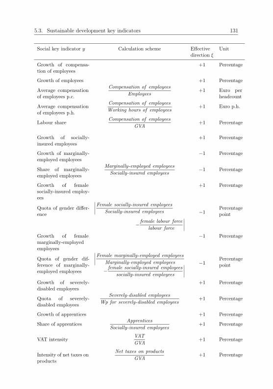
5.3. Sustainable development key indicators 131
Social key indicator y Calculation scheme Effectivedirection ξ
Unit
Growth of compensa-tion of employees
+1 Percentage
Growth of employees +1 Percentage
Average compensationof employees p.c.
Compensation of employees
Employees+1 Euro per
headcount
Average compensationof employees p.h.
Compensation of employees
Working hours of employees+1 Euro p.h.
Labour shareCompensation of employees
GVA+1 Percentage
Growth of socially-insured employees
+1 Percentage
Growth of marginally-employed employees
−1 Percentage
Share of marginally-employed employees
Marginally-employed employees
Socially-insured employees−1 Percentage
Growth of femalesocially-insured employ-ees
+1 Percentage
Quota of gender differ-ence
∣∣∣∣Female socially-insured employees
Socially-insured employees −1Percentagepoint
− female labour force
labour force
∣∣∣∣Growth of femalemarginally-employedemployees
−1 Percentage
Quota of gender dif-ference of marginally-employed employees
∣∣∣∣Female marginally-employed employees
Marginally-employed employees −1Percentagepoint
− female socially-insured employees
socially-insured employees
∣∣∣∣Growth of severely-disabled employees
+1 Percentage
Quota of severely-disabled employees
Severely-disabled employees
Wp for severely-disabled employees+1 Percentage
Growth of apprentices +1 Percentage
Share of apprenticesApprentices
Socially-insured employees+1 Percentage
VAT intensityVAT
GVA+1 Percentage
Intensity of net taxes onproducts
Net taxes on products
GVA+1 Percentage

132 Chapter 5. Empirical findings
continued
Social key indicator y Calculation scheme Effectivedirection ξ
Unit
CIT intensityCIT
GVA+1 Percentage
Local business tax in-tensity
Local business tax
GVA+1 Percentage
Table 5.6 Social key indicators and their characterisation; CIT, Corporate Income Tax; GVA,Gross Value Added; p.c., per capita; p.h., per hour; VAT, Value Added Tax; Wp,Workplaces
be in force (SDG 1.3). Hence, the key figures socially-insured employees and marginally-
employed employees are gathered. Their growth indicators yg comprise the growth of
socially-insured employees and the growth of marginally-employed employees, with the
resulting ratio indicator share of marginally-employed employees (SDG 1.3.1). The
effective directions ξ of the growth and the share of marginally-employed employees are
negative: Marginally-employed employees are not covered by social security systems
(see Section 5.2.1; BA, 2019), and thus, employees should be prevented from this type
of employment.
Supporting SDG 10.2 and SDG 10.3 on inclusion and equal opportunities, discrimin-
ation against all women and girls should be ended (SDG 5.1). Assessing meso-economic
and macro-economic objects’ contributions to these targets, data on female socially-
insured employees, (female) labour force, and female marginally-employed employees
are collected. Growth indicators yg encompass the growth of female socially-insured em-
ployees and the growth of female marginally-employed employees. Because the (female)
labour force is composed of the working population and unemployed people, its growth
rate is only meaningful for overall economies and hence not implied in the MLSDI.
Ratio indicators yr are the quota of gender difference (SDG 16.7.1) and the quota of
gender difference of marginally-employed employees (SDG 1.3.1). Calculation schemes
of the quotas of gender differences are displayed in Table 5.6. The first parts of the
differences represent the status of employment by gender in percentage. The second
parts of the differences indicate possibilities of employment by gender with regard to the
first parts of the equations: The share of female labour force represents the population
of the share of female socially-insured employees, and the share of socially-insured em-
ployees constitute the population of the share of female marginally-employed employees.
Because equality is aimed at (SDG 10.2; SDG 10.3), neither men nor women should be
privileged, and absolute values are taken. Moreover, striving for equality, an increase of
the quotas of gender differences degrade social development, such that their effective
directions ξ are negative.
Continuing to operationalise empowerment and equal opportunities for all (SDG

5.3. Sustainable development key indicators 133
10.2; SDG 10.3), the key figures severely-disabled employees and workplaces for severely-
disabled employees are gathered. The growth of severely-disabled employees and the
quota of severely-disabled employees (SDG 16.7.1) are computed to measure meso-
economic and macro-economic objects’ contributions to these targets. Growth of
workplaces for severely-disabled employees is not calculated because these workplaces
depend on the type and the size of an employer (see Section 5.2.1; BA, 2018). This fixed
calculation scheme prevents individual performances, and the key figure workplaces for
severely-disabled employees only serves standardisation.
Equal access to vocational education (SDG 4.3) and the increase in number of youths
and adults who possess vocational skills (SDG 4.4) should be endeavoured. The key
figure apprentices is gathered, and its key indicators growth of apprentices and share of
apprentices are computed to assess meso and macro contributions to the aforementioned
targets. The share of apprentices is the proportion of apprentices in socially-insured
employees (see Table 5.6).
Fiscal instruments are demanded for reaching social development (SDG 10.4). The
data collection for this target results in the key figures VAT (GRI 201-1), net taxes on
products (GRI 201-1), CIT (GRI 201-1), and local business tax (GRI 201-1). Their
ratio indicators yr are intensities (see Table 5.6) that state the share of GVA passed
to the government. These taxes’ growth indicators yg are excluded from the MLSDI
because, similar to the environmental tax, their growth would not reveal effectiveness
of the taxation system but an increase in the tax bases and economic activity, which is
not part of sustainable development (see Section 2.2.3; e.g. Jackson, 2009).
The next section, Section 5.3.1.3, derives the MLSDI’s economic key indicators y.
5.3.1.3 Economic sustainable development key indicators
The economic domain’s alignment of GRI and SDG disclosures results in key indicators y
that mainly strive for economic productivity. Enhancements of economic key indicators
y imply improved sustainable development performances. Their effective directions
ξ are positive. Because economic growth is only required to eliminate poverty (see
Section 2.2.3; e.g. WCED, 1987), and Germany is one of the seven major economies of
the world (see Section 5.3.1.2; UN, 2019c), economic growth indicators yg are disregarded
for the present sample. One exemption is made: The growth of working population is
investigated as it contributes – jointly with the key indicators y on employment of the
social domain – to the achievement of full and productive employment as well as decent
work for all (SDG 8.5; see Section 5.3.1.2).
To increase economic productivities, technological upgrading should be accomplished
(SDG 8.2). To this end, the key figures gross fixed assets (IAS 16.73d), net fixed assets
(IAS 1.54), consumption of fixed capital (IAS 1.102; IAS 1.103; IAS 1.104), and gross
fixed capital formation (IAS 7.21) are collected. The MLSDI’s resulting ratio indicators

134 Chapter 5. Empirical findings
Economic key indicator y Calculation scheme Effectivedirection ξ
Unit
Gross capital productiv-ity
GVA
Gross fixed assets+1 Percentage
Net capital productivityGVA
Net fixed assets+1 Percentage
Degree of modernityNet fixed assets
Gross fixed assets+1 Percentage
Consumed capital pro-ductivity
GVA
Consumption of fixed capital+1 Percentage
Investment intensityGross fixed capital formation
GVA+1 Percentage
Internal R&D intensityInternal R&D expenditures
GVA+1 Percentage
Share of R&D employeesR&D employees
Employees+1 Percentage
GVA rateGVA
Output+1 Percentage
Growth of working popu-lation
+1 Percentage
Labour productivity p.c.GVA
Working population+1 Euro per head-
count
Labour productivity p.h.GVA
Working hours of WP+1 Euro per hour
Net import intensityImport − export
GVA+1 Percentage
Share of imported inputImported input
Input+1 Percentage
Table 5.7 Economic key indicators and their characterisation; GVA, Gross Value Added;p.c., per capita; p.h., per hour; R&D, Research and Development; WP, WorkingPopulation
yr read: gross capital productivity, net capital productivity, degree of modernity, consumed
capital productivity, and investment intensity. The gross capital productivity indicates
the value of the factor input gross fixed assets to realise GVA (see Table 5.7). The
other productivity indicators of the economic domain function analogically. The gross
fixed capital formation’s ratio indicator yr is an intensity. The degree of modernity
is the ratio of net and gross fixed assets, shedding light on the process of ageing as
it represents the share of fixed assets that has not been consumed (Schmalwasser &
Weber, 2012).
Targeting productivity through innovation (SDG 8.2), data on internal R&D ex-

5.3. Sustainable development key indicators 135
penditures (IAS 38.126; IAS 38.127) and R&D employees are collected. Technological
knowledge may result in future economic benefits (IASB, 2018). The computed ratio in-
dicators yr are internal R&D intensity (SDG 9.5.1) and share of R&D employees (SDG
9.5.2). Because R&D is an investment (Schmalwasser & Weber, 2012), its intensity
instead of productivity is computed.
Additionally, SDG 8.2 suggests emphasising high value-added sectors. The key figure
output is gathered for the computation of the GVA rate, which states the proportion of
GVA in the output.
Labour-intensive sectors should be focused to achieve higher levels of economic
productivity (SDG 8.2). The key figures working population and working hours of
working population are collected to compute the key indicators growth of working
population (SDG 8.5; see Section 5.3.1.2), labour productivity p.c. (SDG 8.2.1), and
labour productivity p.h.
As a last topic of the economic domain, international trade is considered. To
strengthen developing countries, reduction of poverty (SDG 1.2; see Section 5.3.1.2)
and enablement of decent work (SDG 8.5; see Section 5.3.1.2) should be targeted by
significantly increasing exports of these countries (SDG 17.11). From Germany’s point
of view, imports from developing countries should be augmented because Germany
is one of the major seven world economies (see Section 5.3.1.2; UN, 2019c). The key
figures import, export, and imported input are collected to calculate the following
ratio indicators yr: net import intensity and share of imported input. Their calculation
schemes are indicated in Table 5.7.
To sum up, the MLSDI comprises several ratio indicators yr and several growth
indicators yg to map efficiency and effectiveness. From the 36 acquired key figures
x, 30 ratio indicators yr are computed of which six belong to the environmental, 12
to the social, and another 12 to the economic domain. The total number of growth
indicators Yg amounts to 14, with five environmental, eight social, and one economic
growth indicator yg. The number of ratio indicators Yr and growth indicators Yg as well
as the number of key indicators Y across the contentual domains are unbalanced. The
environmental domain contains 11, the social domain is built by 20, and the economic
domain consists of 13 key indicators y. The total number of key indicators Y amounts
to 44. Due to limitations on data availabilities for economic objects n at two-digit level,
several topics could not be included in the MLSDI.
Concluding on Section 5.3.1.1 to Section 5.3.1.3, several SDG targets are repetitively
stated and measured by more than one key indicator y. Moreover, SDG targets do
not always follow their goals’ assignment to the contentual domains (e.g. Folke et al.,
2016). For instance, a target that belongs to a social goal might be assigned to the
environmental domain. Especially the environmental domain connects all three domains:
Environmental efficiency regards the environmental and the economic domains, and
health-related issues caused by environmental degradation concern the environmental
136 Chapter 5. Empirical findings
and the social domains. Other examples have been provided in Section 2.2.4. These find-
ings verify the interconnectedness of the goals and strengthen the assessment principle
synergies and trade-offs (see Section 3.1; e.g. Costanza, Fioramonti & Kubiszewski, 2016)
to be tackled by the MLSDI’s weighting procedure (see Section 4.3.7 and Section 5.4).
The following section, Section 5.3.2, describes and analyses the summary statistics
of the growth indicators yg.
5.3.2 Summary statistics of the sustainable development
growth indicators
At this stage of the calculation, the key indicators y are unscaled and not comparable to
each other. However, growth indicators yg are uniformly reported in percentages, and
their empirical results reveal greater insights when unscaled: Their signs indicate the
direction of change. The direction of change is desired to be in line with the effective
direction ξ. For example, positively affecting key indicators y are desired to exhibit
positive growth rates. Rescaled growth indicators ygs trade this straightforwardness
for comparability to rescaled ratio indicators yrs (see Section 4.3.6.2) and subsequent
aggregation (see Section 4.3.8). Therefore, summary statistics of the unscaled growth
indicators yg are analysed in this section before the scaling procedure. Outlying key
indicators yo are untreated, but conclusions of this analysis remain valid as growth
indicators yg are characterised by a relatively low outlier rate β (see Section 5.3.3). Full
summary statistics of both the unscaled growth indicators yg and the unscaled ratio
indicators yr are provided in the Appendix A.4, Table A.6 to Table A.8.
Summary statistics classify a distribution according to its centre, spread or dispersion,
and frequency. Central measures to be analysed are the mean and median. High central
measures are endeavoured for key indicators y that feature a positive effective direction
ξ+. Common measures of dispersion are the standard deviation, median absolute
deviation, minimum, maximum, and the 25th and the 75th percentiles. Neither the
standard deviation nor the median absolute deviation are included in the analysis
because deviations from central measures are not crucial in sustainable development
assessment, but deviations from targets should be quantified (see Section 3.1; e.g. Sala
et al., 2015). Owing to lacks in data, targets could not be included but are replaced by
distributional minima and maxima (see Section 4.3.6.2). Changes in the extremes signal
alteration in the performance of the worst and the best economic object n, respectively.
If a key indicator’s effective direction ξ is positive, an increase in the extremes is desired.
The 25th and the 75th percentiles are of interest in order to localise the interior 50%
of the distribution. Analysed frequency measures are skewness and kurtosis. The
relation of the mean and the median raise expectations about the skewness. If the mean
exceeds the median, frequent values occur at the bottom, such that the distribution
is positively (right) skewed. Vice versa, if the median surpasses the mean, frequent

5.3. Sustainable development key indicators 137
Environmental growth indicator ygYear Mean Median Min Max Q1 Q3 Skewness Kurtosis
Growth of air emissions
2008-2016 -0.0197 -0.0560 -0.5725 0.8553 -0.1543 0.1370 0.6864 1.0852
Growth of primary energy consumption
2008-2016 -0.0158 -0.0479 -0.4671 0.5762 -0.1336 0.0803 0.5046 0.5235
Growth of water use
2008-2016 -0.0096 -0.0049 -0.6255 0.6064 -0.1261 0.1022 0.0996 1.0119
Growth of waste water
2008-2016 -0.0304 -0.0098 -1.0000 0.6045 -0.1407 0.0870 -0.6825 2.6684
Growth of hazardous waste
2008-2016 -0.0607 -0.0969 -0.6637 1.4894 -0.2958 0.1581 1.2043 2.6282
Table 5.8 Summary statistics of the environmental growth indicators in the German economyfrom 2008 to 2016; Max, Maximum; Min, Minimum; Q1, 25
th percentile; Q3, 75th
percentile
scores are located at the top, entailing negative (left) skewness. These rules on resulting
skewness hold true in most but not all cases (von Hippel, 2005). A distribution is fairly
symmetrical if absolute skewness remains below 0.5. Moderate skewness ranges between
absolute values of 0.5 to 1.0, and distributions with absolute skewness higher than
1.0 are highly skewed (Bulmer, 1979). Negatively skewed distributions are favourable
for sustainable development. In this case, light tails (negative kurtosis) are desired
because the tail refers to the bottom of the distribution. The opposite is preferred
for positively skewed distributions, such that the kurtosis is ambiguous for sustainable
development. A distribution is platykurtic (light tails) for kurtosis values below −2.0,
mesokurtic (normal) for scores between −2.0 and 2.0, and leptokurtic (heavy tails) for
values above 2.0 (George & Mallery, 2005). If sustainability is reached, the distribution
of key indicators y will be non-normal (Schmidt-Traub et al., 2017b). All statements can
be reverted for key indicators y that have a negative effect on sustainable development.
Summary statistics of the growth indicators yg are provided in Table 5.8 for the
environmental domain and in Table 5.9 for the social and the economic domains.
Central measures of the environmental domain’s growth indicators yg are negative (see
Table 5.8). Given their negative effective direction ξ−, this finding is desirable with
regard to improved environmental effectiveness, supporting a variety of SDGs (see
Section 5.3.1.1). The lowest negative growth rate is obtained for the median growth of
hazardous waste. Median hazardous waste reduced by −9.69% from 2008 to 2016. Its
mean amounts to −6.07%. Moreover, growth of hazardous waste are highly positively
skewed (skewness of 1.20) and leptokurtic (kurtosis of 2.63). Asymmetry is directed
towards the bottom (in favour of environmental protection), but frequent observations
occur in the tails, which approach the top of the distribution. The other key indicators’

138 Chapter 5. Empirical findings
Social or economic growth indicator ygYear Mean Median Min Max Q1 Q3 Skewness Kurtosis
Growth of compensation of employees
2008-2016 0.2581 0.2504 -0.2456 0.7671 0.1438 0.3701 0.0959 0.4252
Growth of employees
2008-2016 0.0426 0.0358 -0.3789 0.4471 -0.0471 0.1495 -0.1090 0.4946
Growth of socially-insured employees
2008-2016 0.0928 0.0735 -0.3922 0.4890 -0.0249 0.1863 0.0227 -0.1974
Growth of marginally-employed employees
2008-2016 -0.1113 -0.1125 -0.4362 0.3536 -0.2603 -0.0006 0.4193 -0.4219
Growth of female socially-insured employees
2008-2016 0.1036 0.1061 -0.4750 0.4394 -0.0154 0.2130 -0.3150 0.5848
Growth of female marginally-employed employees
2008-2016 -0.2078 -0.2056 -0.4707 0.2130 -0.3575 -0.1061 0.4022 -0.7059
Growth of severely-disabled employees
2008-2016 0.2331 0.1962 -0.8048 1.0693 0.0816 0.3610 0.1145 2.3748
Growth of apprentices
2008-2016 -0.0950 -0.0889 -0.6537 0.7309 -0.2206 0.0351 0.4514 2.1157
Growth of working population
2008-2016 0.0254 0.0205 -0.3763 0.3393 -0.0512 0.1129 -0.2320 0.3135
Table 5.9 Summary statistics of the social and economic growth indicators in the Germaneconomy from 2008 to 2016; Max, Maximum; Min, Minimum; Q1, 25
th percentile;Q3, 75
th percentile
growth rates feature moderate positive skewnesses and are mesokurtic. Growth of waste
water is an exception as it is moderately skewed to the left and leptokurtic (undesired).
Results of the central measures of the growth indicators yg of the social and the
economic domains follow their effective directions ξ (see Table 5.9), contributing to
effective achievement of the respective SDGs (see Section 5.3.1.2 and Section 5.3.1.3).
Only the growth of apprentices is not in line with this finding, and its mean and median
are negative with values amounting to −9.50% and −8.89%, respectively. The SDG
target to increase the number of people with vocational skills (SDG 4.4) is missed,
exacerbating the shortage of future skilled workers, which are already missing today
(e.g. Bonin, 2019). The growth of severely-disabled employees experiences the lowest
minimum (−80.48%) and highest maximum (106.93%). Skewnesses and kurtoses of the
social growth indicators yg are mostly negligible and close to be normal. Growth of
severely-disabled employees and apprentices are exceptions with leptokurtic distributions;
their kurtoses amount to 2.37 and 2.12, respectively. Because skewness is negligible,
frequent values occur at both the bottom and the top. Bottom results are desired to be
shifted towards the top.

5.3. Sustainable development key indicators 139
Gram CO2e per Euro
Freq
uenc
y0
100
200
300
400
500
0 2,000 6,000 10,000
HistogramMeanMedianOutlier threshold
(a) Histogram and frequency distribution
●
●
●
●
●
●
●
●
●
●●
●
●
●
●
●●
●
●
●
●
●
●●
●
●●
●
●●
●
●
●●
●
●
●
●
●●
●
●●
●
●
●
●
●
●●
●
●●
●
●●
●
●
●
●
●
●●
●
●
●
●
●●
●
●
●●
●
●●
●
●
●
●●●
●
●
●●
●
●
●
●●
●
●●
●
●
●●
●
●
●
●
●
●
●●
●
●●
●
●
●
●
Gra
m C
O2e
per
Eur
o
0
2,00
04,
000
6,00
08,
000
(b) Boxplot and quartiles
Figure 5.7 Outliers of the air emissions intensity in gram Carbon Dioxide Equivalents (CO2e)in the German economy from 2008 to 2016
The following section, Section 5.3.3, detects and removes outlying key indicators yo.
5.3.3 Outlier detection and treatment
Outlier rates β and degrees of outlyingness are diverse across the three contentual
domains and across ratio indicators yr and growth indicators yg. The environmental
domain suffers most from outlyingness, with an outlier rate β of 10.77% and very strong
outlying key indicators yo especially for ratio indicators yr. The economic domain
exhibits an outlier rate β of 8.66% and diverse degrees of outlyingness, ranging from
none (e.g. GVA rate), weak (e.g. share of imported input), moderate (e.g. investment
intensity), to strong (e.g. labour productivity p.h.). The social domain’s outlier rate β
is the lowest (3.09%), and outlyingness is weak. The outlier rate β of ratio indicators
yr is more than twice as high as the growth indicators’ outlier rate β: 8.06% vs. 3.34%.
Outlier illustration in histograms as displayed earlier in Figure 5.5 may assist
outliers’ visual analysis. However, boxplots are more valuable in this context because
they picture the IQR method. Boxes indicate the IQR q, whiskers denote the product
of the outlier coefficient α and the IQR q, and outliers are expressed by circles. An
exemplary histogram and boxplot of the key indicator air emissions intensity are shown
in Figure 5.7a and Figure 5.7b, respectively. The key indicator air emissions intensity is
chosen due to its exemplariness of the environmental domain. The distribution of the
air emissions intensity is positively skewed (average skewness of 3.16; see Table A.6),
and numerous outlying key indicators yo exist at the top of the distribution. The mean
equals 665.35 gCO2e per Euro, while the median only reaches 65.94 gCO2e per Euro
from 2008 to 2016 (see Table A.6). This finding demonstrates the effect of masking

140 Chapter 5. Empirical findings
Percentage of input
Freq
uenc
y
0.0 0.2 0.4 0.6 0.8
020
4060
8010
012
014
0HistogramMeanMedianOutlier threshold
(a) Histogram and frequency distribution
●
●
●●●
●●
●
●
●
●
●
●
●●
0.0
0.2
0.4
0.6
0.8
Perc
enta
ge o
f inp
ut(b) Boxplot and quartiles
Figure 5.8 Outliers of the share of imported input in percentage of input in the Germaneconomy from 2008 to 2016
and inappropriateness of the mean and measures based on it for outlier detection (see
Section 4.3.5.2; Field, 2009): The vast number of outlying key indicators yo at the top
influence the mean to a degree that it exceeds the upper outlier threshold θmax equal to
619.63 gCO2e per Euro (see Table A.9). Outlier thresholds of each key indicator y can
be found in Table A.9 to Table A.11 in the Appendix A.5.
As a further example, the share of imported input and its weak outlyingness are
chosen (see Figure 5.8). Because outlying key indicators yo are weaker and fewer in
number compared to the air emissions intensity, the box of the boxplot is larger, and
whiskers are longer (see Figure 5.8b). Given the weakness of outlyingness, the mean is
close to the median, not approaching the outlier thresholds θ (see Figure 5.8a).
In both examples, outlying key indicators yo occur at the top of the distribution.
However, outlying key indicators yo at the bottom occur for the key indicators share of
apprentices, VAT intensity, intensity of net taxes on products and net import intensity.
Therefore, a two-sided outlier treatment is required.
After replacing outlying key indicators yo with the respective thresholds θ (see
Table A.9 to Table A.11), key indicators y are rescaled and described along with their
empirical findings in the following section, Section 5.3.4.
5.3.4 Empirical findings of the cleaned and rescaled sustain-
able development key indicators
The rescaled key indicators ys feature positive effective directions ξ+ (see Section 4.3.6.2)
and are free from missing values and outliers (see Figure 4.1). Key indicators y with a
positive effective direction ξ+ retain their labels after scaling, while negatively affecting

5.3. Sustainable development key indicators 141
Key indicator y Rescaled key indicator ys
Growth of air emissions Reduction of air emissions
Air emissions intensity Air emissions efficiency
Growth of primary energy con-sumption
Reduction of primary energy con-sumption
Energy intensity Energy efficiency
Growth of water use Reduction of water use
Water intensity Water efficiency
Growth of waste water Reduction of waste water
Waste water intensity Waste water efficiency
Growth of hazardous waste Reduction of hazardous waste
Hazardous waste intensity Hazardous waste efficiency
Growth of marginally-employed em-ployees
Reduction of marginally-employedemployees
Share of marginally-employed em-ployees
Share of non-marginally-employedemployees
Quota of gender difference Quota of gender equality
Growth of female marginally-employed employees
Reduction of female marginally-employed employees
Quota of gender difference ofmarginally-employed employees
Quota of gender equality ofmarginally-employed employees
Table 5.10 Denotation of negatively affecting key indicators before and after scaling
key indicators’ notations change. Negatively affecting growth indicators yg alter their
denotation from “growth” to “reduction”, environmental ratio indicators yr except the
environmental tax intensity are now reported as efficiencies, the share of marginally-
employed employees is interpreted as non-marginally-employed employees, and gender
differences are translated into gender equalities. The labels are compared in Table 5.10.
The empirical findings of the cleaned and rescaled key indicators ys are analysed in
two manners: Summary statistics are investigated in Section 5.3.4.1, and the selected
branches (see Table 5.1) are analysed in Section 5.3.4.2. The evaluation of the perform-
ance scores follows Prescott-Allen (2001; see Section 4.3.6.2). Scores should be at least
fair to be acceptable. Bad results require actions for improvements.
5.3.4.1 Summary statistics
Interpretations of the summary statistics towards sustainable development (see Sec-
tion 5.3.2) remain valid for rescaled performance scores with one additional aspect:
If a key indicator’s score of the 25th or the 75th percentile is higher than 25.00 (poor
142 Chapter 5. Empirical findings
performance) or 75.00 (fair performance), respectively, it approximately contributes
more to sustainable development than a normally-distributed key indicator y would.51
Therefore, scores exceeding 25.00 and 75.00, respectively, are strived for.
Results of the rescaled growth indicators ygs of the environmental domain (see
Table 5.11) are in line with their unscaled counterparts analysed in Section 5.3.2.
Distributional properties among the rescaled environmental growth indicators ygs are
relatively homogeneous. The economic objects n exhibit a medium central (mean and
median) performance of environmental effectiveness. Only the median reduction of air
emissions and both mean and median reduction of hazardous waste score fair results.
The outstanding median reduction of hazardous waste of −9.69% (see Section 5.3.2) is
converted into a score of 67.04, a fair and acceptable performance. Rescaled environ-
mental ratio indicators yrs yield fair mean performances and good median performances
(see Table 5.11). Central measures generally show stable, increasing trends. This is a
positive finding for environmental efficiency as relative decoupling of environmental
degradation and economic activity (SDG 8.4) is centrally achieved. The biggest increase
in central environmental efficiency occurs for the hazardous waste efficiency’s mean: It
increased from 72.60 in 2008 to 77.67 in 2016, which corresponds to a growth rate of
6.98%. Because the median only increased by 2.40%, it is supposed that the mean’s
increase is caused by few economic objects n. Enhancements by further economic objects
n are desirable. The improvement of the hazardous waste efficiency is followed by the
waste water efficiency’s mean, which grew by 6.57% from 2008 to 2016. Concerning the
25th and the 75th percentiles, 50% of the distribution is shifted upward by one bracket:
Instead of the normal poor to fair performances, at least medium to good performances
are reached by 50% of the distribution, respectively. As a result, the distributions are
mostly highly negatively skewed. Kurtoses are mostly negative but relatively small
and negligible. Not in favour of environmental protection are the extremes as they are
nearly invariant over time without improvements. Constant extremes appear due to
outlier treatment. The environmental tax intensity is an exception to these findings. Its
central outcomes are poor to medium, the 25th and the 75th percentiles are below those
of a normal distribution, and the data are highly positively skewed. Improvements over
time are reported but insignificant.
Rescaled key indicators ys of the social domain are more diverse than those of the
environmental domain (see Table 5.12). Central measures feature wider ranges (poor to
good), their trends are increasing as well as decreasing, and skewnesses and kurtoses are
both positive and negative. The rescaled growth indicators ygs of the compensation of
employees and employees achieve medium results with a rather normal shape. Average
compensations of employees (p.c. and p.h.) exhibit central performances at the lower
end of being medium. However, the average compensations of employees’ minima
51The contribution is only “approximately” higher because key indicators y are not rescaled on aninterval from zero to 100 but ten to 100.

5.3. Sustainable development key indicators 143
Rescaled environmental key indicator ysYear Mean Median Min Max Q1 Q3 Skewness Kurtosis
Reduction of air emissions
2008-2016 58.22 63.85 10.00 100.00 44.49 72.06 -0.3345 -0.4290
Air emissions efficiency
2008 70.89 89.35 10.00 99.88 60.46 93.54 -1.0737 -0.6268
2009 70.85 90.46 10.00 99.95 56.69 94.19 -1.0485 -0.6845
2010 70.87 90.43 10.00 99.95 59.28 93.89 -1.0516 -0.6745
2011 71.78 91.44 10.00 100.00 62.00 94.78 -1.0974 -0.5997
2012 72.15 91.44 10.00 99.98 62.46 94.76 -1.1186 -0.5604
2013 72.02 91.83 10.00 99.99 63.08 94.74 -1.1107 -0.5659
2014 72.71 92.33 10.00 99.98 62.19 94.68 -1.1202 -0.5494
2015 72.83 92.14 10.00 99.93 62.67 94.93 -1.1307 -0.5177
2016 73.08 92.01 10.00 99.90 59.82 94.98 -1.1149 -0.5618
Reduction of primary energy consumption
2008-2016 52.44 56.09 10.00 100.00 37.24 66.25 -0.0612 -0.4713
Energy efficiency
2008 69.71 87.81 10.00 99.88 57.25 90.93 -1.0431 -0.5586
2009 69.34 89.00 10.00 99.93 52.79 91.96 -1.0083 -0.6775
2010 69.36 87.87 10.00 99.89 57.34 91.00 -1.0208 -0.6160
2011 70.85 89.63 10.00 100.00 62.50 92.40 -1.0941 -0.4749
2012 71.51 89.44 10.00 99.93 64.31 92.99 -1.1516 -0.3423
2013 71.21 89.40 10.00 99.97 60.13 92.70 -1.1109 -0.4305
2014 72.29 90.09 10.00 99.99 62.33 93.38 -1.1503 -0.3136
2015 72.13 90.42 10.00 99.91 64.57 93.26 -1.1553 -0.3463
2016 72.53 91.14 10.00 99.92 66.13 93.55 -1.1788 -0.2861
Reduction of water use
2008-2016 51.13 52.51 10.00 100.00 35.85 65.80 -0.0164 -0.5466
Water efficiency
2008 72.43 91.57 10.00 100.00 56.70 97.26 -1.0635 -0.5928
2009 71.66 90.25 10.00 99.99 54.04 97.44 -1.0257 -0.6702
2010 72.41 91.25 10.00 99.99 54.54 97.20 -1.0657 -0.6007
2011 73.30 92.03 10.00 100.00 62.02 97.10 -1.1311 -0.4504
2012 73.70 91.46 10.00 99.99 65.29 96.98 -1.1675 -0.3766
2013 74.40 91.21 10.00 99.99 67.93 97.12 -1.2155 -0.2894
2014 74.58 91.80 10.00 99.99 67.96 97.40 -1.2268 -0.2490
2015 75.04 92.05 10.00 100.00 70.46 97.54 -1.2513 -0.2143
2016 75.28 92.54 10.00 100.00 72.20 97.54 -1.2709 -0.1668
Reduction of waste water
2008-2016 51.68 52.18 10.00 100.00 38.61 64.72 0.0602 -0.5638
Waste water efficiency
2008 69.56 85.49 10.00 100.00 58.57 95.47 -0.9662 -0.6636
2009 68.59 84.46 10.00 100.00 48.54 95.15 -0.8927 -0.8238
2010 69.62 84.23 10.00 100.00 56.87 95.51 -0.9752 -0.6576
2011 70.79 85.59 10.00 100.00 61.70 95.73 -1.0432 -0.4924
2012 71.38 85.15 10.00 100.00 62.68 95.80 -1.0941 -0.3422
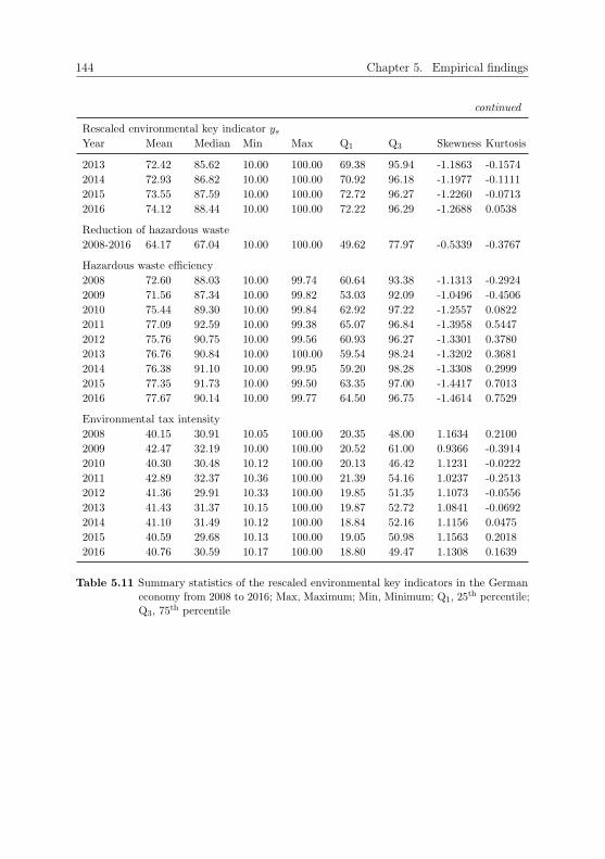
144 Chapter 5. Empirical findings
continued
Rescaled environmental key indicator ysYear Mean Median Min Max Q1 Q3 Skewness Kurtosis
2013 72.42 85.62 10.00 100.00 69.38 95.94 -1.1863 -0.1574
2014 72.93 86.82 10.00 100.00 70.92 96.18 -1.1977 -0.1111
2015 73.55 87.59 10.00 100.00 72.72 96.27 -1.2260 -0.0713
2016 74.12 88.44 10.00 100.00 72.22 96.29 -1.2688 0.0538
Reduction of hazardous waste
2008-2016 64.17 67.04 10.00 100.00 49.62 77.97 -0.5339 -0.3767
Hazardous waste efficiency
2008 72.60 88.03 10.00 99.74 60.64 93.38 -1.1313 -0.2924
2009 71.56 87.34 10.00 99.82 53.03 92.09 -1.0496 -0.4506
2010 75.44 89.30 10.00 99.84 62.92 97.22 -1.2557 0.0822
2011 77.09 92.59 10.00 99.38 65.07 96.84 -1.3958 0.5447
2012 75.76 90.75 10.00 99.56 60.93 96.27 -1.3301 0.3780
2013 76.76 90.84 10.00 100.00 59.54 98.24 -1.3202 0.3681
2014 76.38 91.10 10.00 99.95 59.20 98.28 -1.3308 0.2999
2015 77.35 91.73 10.00 99.50 63.35 97.00 -1.4417 0.7013
2016 77.67 90.14 10.00 99.77 64.50 96.75 -1.4614 0.7529
Environmental tax intensity
2008 40.15 30.91 10.05 100.00 20.35 48.00 1.1634 0.2100
2009 42.47 32.19 10.00 100.00 20.52 61.00 0.9366 -0.3914
2010 40.30 30.48 10.12 100.00 20.13 46.42 1.1231 -0.0222
2011 42.89 32.37 10.36 100.00 21.39 54.16 1.0237 -0.2513
2012 41.36 29.91 10.33 100.00 19.85 51.35 1.1073 -0.0556
2013 41.43 31.37 10.15 100.00 19.87 52.72 1.0841 -0.0692
2014 41.10 31.49 10.12 100.00 18.84 52.16 1.1156 0.0475
2015 40.59 29.68 10.13 100.00 19.05 50.98 1.1563 0.2018
2016 40.76 30.59 10.17 100.00 18.80 49.47 1.1308 0.1639
Table 5.11 Summary statistics of the rescaled environmental key indicators in the Germaneconomy from 2008 to 2016; Max, Maximum; Min, Minimum; Q1, 25
th percentile;Q3, 75
th percentile

5.3. Sustainable development key indicators 145
Rescaled social key indicator ysYear Mean Median Min Max Q1 Q3 Skewness Kurtosis
Growth of compensation of employees
2008-2016 55.10 54.35 10.00 100.00 43.96 65.94 0.0939 0.0603
Growth of employees
2008-2016 54.09 53.24 10.00 100.00 44.13 65.89 -0.0425 0.2290
Average compensation of employees p.c.
2008 40.96 39.15 10.00 80.45 28.48 56.10 0.1618 -1.0535
2009 41.51 38.40 10.35 84.16 28.55 58.63 0.2776 -0.9296
2010 42.82 40.35 10.85 82.01 28.85 59.86 0.2001 -1.0649
2011 44.74 41.87 11.36 87.96 29.84 60.93 0.2900 -0.9443
2012 45.70 42.88 11.77 97.06 30.40 61.16 0.3135 -0.8280
2013 46.75 43.79 11.94 90.55 31.41 62.40 0.2494 -1.0653
2014 48.25 45.04 12.78 90.94 32.21 64.56 0.2231 -1.1074
2015 50.14 46.08 13.98 100.00 34.46 66.48 0.2900 -1.0037
2016 51.40 47.93 14.71 96.96 36.63 68.18 0.2942 -0.9838
Average compensation of employees p.h.
2008 39.33 35.10 10.00 73.28 27.60 54.20 0.3180 -1.0283
2009 42.43 37.41 10.86 90.76 29.62 58.64 0.4109 -0.8332
2010 43.00 37.44 11.18 86.30 30.29 60.64 0.3181 -0.9929
2011 44.73 38.30 13.03 88.76 31.42 61.13 0.3625 -0.9759
2012 46.87 40.52 13.62 98.81 33.74 63.29 0.3956 -0.8187
2013 48.20 40.66 15.13 91.62 35.01 65.22 0.3986 -0.9901
2014 49.68 41.67 15.98 96.57 36.03 67.58 0.4191 -0.9604
2015 51.49 43.40 16.49 100.00 37.13 69.66 0.4234 -0.9610
2016 53.33 46.25 18.40 96.70 39.47 73.24 0.4256 -0.9522
Labour share
2008 58.82 61.95 10.02 96.06 44.82 72.46 -0.3736 -0.4180
2009 62.17 67.43 10.04 97.90 46.00 77.95 -0.5212 -0.4225
2010 59.95 63.67 10.07 97.28 45.18 72.32 -0.4230 -0.3094
2011 59.94 64.24 10.00 96.02 43.20 71.04 -0.3408 -0.3462
2012 60.37 63.73 10.19 94.97 44.67 72.08 -0.4006 -0.3166
2013 60.38 64.15 10.01 95.52 43.65 73.54 -0.5000 -0.3311
2014 60.46 63.79 10.16 95.11 44.57 72.88 -0.4271 -0.3507
2015 59.79 63.64 10.20 97.36 45.58 71.62 -0.3987 -0.2410
2016 60.07 61.75 10.35 100.00 47.11 72.32 -0.2688 -0.2626
Growth of socially-insured employees
2008-2016 57.16 54.98 10.00 100.00 44.55 67.13 0.0932 -0.4334
Reduction of marginally-employed employees
2008-2016 65.70 67.10 10.00 100.00 52.45 85.03 -0.4750 -0.6180
Share of non-marginally-employed employees
2008 70.67 80.26 10.00 99.59 58.61 93.43 -1.0404 -0.1308
2009 70.75 80.45 10.00 99.73 59.39 93.64 -1.0340 -0.1559
2010 71.17 80.85 10.00 99.65 59.18 93.64 -1.0569 -0.1071
2011 71.70 81.53 10.00 99.79 59.40 94.08 -1.0819 -0.0465
2012 72.21 82.14 10.00 99.83 60.32 94.24 -1.1094 0.0189

146 Chapter 5. Empirical findings
continued
Rescaled social key indicator ysYear Mean Median Min Max Q1 Q3 Skewness Kurtosis
2013 72.41 82.23 10.00 99.81 60.62 94.12 -1.1304 0.0585
2014 72.86 82.41 10.00 99.87 61.00 93.85 -1.1447 0.1019
2015 74.19 83.16 10.00 99.98 62.59 93.78 -1.2147 0.3628
2016 74.93 83.89 10.00 100.00 63.68 93.47 -1.2612 0.5464
Growth of female socially-insured employees
2008-2016 62.31 62.38 10.00 100.00 48.82 74.43 -0.0535 -0.3389
Quota of gender equality
2008 54.94 54.69 10.00 97.40 34.36 74.31 0.0409 -1.1385
2009 55.00 53.83 10.53 98.94 34.44 75.11 0.0487 -1.1417
2010 54.89 54.57 11.09 99.01 34.77 75.48 0.0669 -1.1529
2011 54.56 54.59 10.92 98.77 33.95 73.97 0.1088 -1.1442
2012 54.79 54.46 12.07 99.06 34.49 73.34 0.1108 -1.1364
2013 54.86 54.13 12.40 98.55 34.18 73.47 0.0958 -1.1526
2014 54.95 54.64 13.30 99.50 34.02 73.55 0.0886 -1.1746
2015 55.09 55.29 13.90 99.65 33.64 73.89 0.0872 -1.1878
2016 55.42 56.30 13.99 99.96 33.58 74.05 0.0956 -1.1772
Reduction of female marginally-employed employees
2008-2016 65.39 65.11 10.00 100.00 52.39 85.07 -0.3935 -0.7714
Quota of gender equality of marginally-employed employees
2008 62.42 60.80 10.00 98.23 48.47 78.87 0.0031 -0.4813
2009 63.30 61.69 10.00 98.56 50.17 80.27 -0.0981 -0.4790
2010 64.27 62.71 11.94 98.88 50.74 81.11 -0.0994 -0.5372
2011 65.58 63.97 16.71 99.27 51.91 80.51 -0.0937 -0.5829
2012 66.91 65.05 24.59 99.95 52.71 81.57 -0.0350 -0.8109
2013 68.32 66.65 28.05 98.27 54.81 82.73 -0.0376 -0.8852
2014 69.72 68.35 32.45 99.41 56.58 83.32 -0.0544 -0.9419
2015 72.06 72.00 38.38 99.55 58.56 84.97 0.0667 -1.0547
2016 73.26 72.37 39.89 100.00 59.68 85.40 0.0788 -1.0101
Growth of severely-disabled employees
2008-2016 55.80 52.98 10.00 100.00 43.82 65.80 0.4418 0.0470
Quota of severely-disabled employees
2008 51.64 52.78 10.00 92.93 40.25 61.82 0.1020 0.0099
2009 54.12 54.61 15.66 97.60 42.52 64.08 0.2105 0.0382
2010 55.45 56.06 13.82 100.00 42.87 65.19 0.2147 -0.0128
2011 55.45 56.09 15.39 100.00 43.50 64.93 0.0945 -0.0054
2012 56.81 57.29 19.28 100.00 44.99 66.31 0.1780 -0.1356
2013 57.61 58.92 20.43 100.00 45.64 66.62 0.0944 -0.2096
2014 57.77 58.84 20.37 100.00 45.49 67.20 0.2036 -0.2337
2015 58.26 60.35 20.35 100.00 44.55 67.51 0.1971 -0.4598
2016 57.64 59.44 20.49 98.37 44.49 67.80 0.1085 -0.5001
Growth of apprentices
2008-2016 55.59 55.76 10.00 100.00 44.15 66.35 0.0705 0.0546
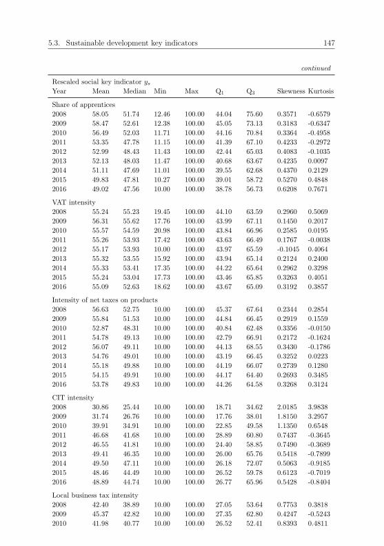
5.3. Sustainable development key indicators 147
continued
Rescaled social key indicator ysYear Mean Median Min Max Q1 Q3 Skewness Kurtosis
Share of apprentices
2008 58.05 51.74 12.46 100.00 44.04 75.60 0.3571 -0.6579
2009 58.47 52.61 12.38 100.00 45.05 73.13 0.3183 -0.6347
2010 56.49 52.03 11.71 100.00 44.16 70.84 0.3364 -0.4958
2011 53.35 47.78 11.15 100.00 41.39 67.10 0.4233 -0.2972
2012 52.99 48.43 11.43 100.00 42.44 65.03 0.4083 -0.1035
2013 52.13 48.03 11.47 100.00 40.68 63.67 0.4235 0.0097
2014 51.11 47.69 11.01 100.00 39.55 62.68 0.4370 0.2129
2015 49.83 47.81 10.27 100.00 39.01 58.72 0.5270 0.4848
2016 49.02 47.56 10.00 100.00 38.78 56.73 0.6208 0.7671
VAT intensity
2008 55.24 55.23 19.45 100.00 44.10 63.59 0.2960 0.5069
2009 56.31 55.62 17.76 100.00 43.99 67.11 0.1450 0.2017
2010 55.57 54.59 20.98 100.00 43.84 66.96 0.2585 0.0195
2011 55.26 53.93 17.42 100.00 43.63 66.49 0.1767 -0.0038
2012 55.17 53.93 10.00 100.00 43.97 65.59 -0.1045 0.4064
2013 55.32 53.55 15.92 100.00 43.94 65.14 0.2124 0.2400
2014 55.33 53.41 17.35 100.00 44.22 65.64 0.2962 0.3298
2015 55.24 53.04 17.73 100.00 43.46 65.85 0.3263 0.4051
2016 55.09 52.63 18.62 100.00 43.67 65.09 0.3192 0.3857
Intensity of net taxes on products
2008 56.63 52.75 10.00 100.00 45.37 67.64 0.2344 0.2854
2009 55.84 51.53 10.00 100.00 44.84 66.45 0.2919 0.1559
2010 52.87 48.31 10.00 100.00 40.84 62.48 0.3356 -0.0150
2011 54.78 49.13 10.00 100.00 42.79 66.91 0.2172 -0.1624
2012 56.07 49.11 10.00 100.00 44.13 68.55 0.3430 -0.1786
2013 54.76 49.01 10.00 100.00 43.19 66.45 0.3252 0.0223
2014 55.18 49.88 10.00 100.00 44.19 66.07 0.2739 0.1280
2015 54.15 49.91 10.00 100.00 44.17 64.40 0.2693 0.3485
2016 53.78 49.83 10.00 100.00 44.26 64.58 0.3268 0.3124
CIT intensity
2008 30.86 25.44 10.00 100.00 18.71 34.62 2.0185 3.9838
2009 31.74 26.76 10.00 100.00 17.76 38.01 1.8150 3.2957
2010 39.91 34.91 10.00 100.00 22.85 49.58 1.1350 0.6548
2011 46.68 41.68 10.00 100.00 28.89 60.80 0.7437 -0.3645
2012 46.55 41.81 10.00 100.00 24.40 58.85 0.7490 -0.3689
2013 49.41 46.35 10.00 100.00 26.00 65.76 0.5418 -0.7899
2014 49.50 47.11 10.00 100.00 26.18 72.07 0.5063 -0.9185
2015 48.46 44.49 10.00 100.00 26.52 59.78 0.6123 -0.7019
2016 48.89 44.74 10.00 100.00 26.77 65.96 0.5428 -0.8404
Local business tax intensity
2008 42.40 38.89 10.00 100.00 27.05 53.64 0.7753 0.3818
2009 45.37 42.82 10.00 100.00 27.35 62.80 0.4247 -0.5243
2010 41.98 40.77 10.00 100.00 26.52 52.41 0.8393 0.4811

148 Chapter 5. Empirical findings
continued
Rescaled social key indicator ysYear Mean Median Min Max Q1 Q3 Skewness Kurtosis
2011 46.01 44.98 10.00 100.00 30.17 59.59 0.5739 -0.1319
2012 46.57 45.57 10.00 100.00 28.03 57.67 0.5841 -0.3130
2013 45.13 44.71 10.00 100.00 27.22 55.40 0.4980 -0.1700
2014 45.80 46.26 10.00 100.00 27.47 56.07 0.5600 -0.2632
2015 45.12 45.58 10.00 100.00 27.90 54.34 0.6508 0.0884
2016 44.96 45.62 10.00 100.00 28.15 55.86 0.6750 0.1738
Table 5.12 Summary statistics of the rescaled social key indicators in the German economyfrom 2008 to 2016; CIT, Corporate Income Tax; Max, Maximum; Min, Minimum;p.c., per capita; p.h., per hour; Q1, 25
th percentile; Q3, 75th percentile; VAT,
Value Added Tax
experienced increases of 47.13% and 83.98%, respectively, and the 25th percentiles
advanced by 28.62% and 43.00%, respectively, from 2008 to 2016. Contributions to the
SDG target of sustaining income growth of the bottom 40% are made (SDG 10.1). The
labour share yields higher performances with mostly fair central measures. The IQR is
reduced over time, and the GVA distributed to employees becomes more homogeneous
across economic objects n. Central reduction of marginally-employed employees as
well as the mean share of non-marginally-employed employees achieve fair results.
Additionally, the latter rescaled key indicator ys steadily increases its performance, and
its medians are appraised with good. The 25th and the 75th percentiles exceed those of a
normal distribution, and 75% of the economic objects n perform at least medium (58.61
in 2008). This leads to a highly negatively skewed distribution with skewness amounting
to −1.26 in 2016. This is favourable for implementation of social protection systems
(SDG 1.3). Economic objects n perform fair in central rescaled growth indicators ygs on
female employees and the quota of gender equality of marginally-employed employees.
In contrast, medium results are reported for the quota of gender equality. The quota of
gender equality should be enhanced. However, marginal employment is more critical in
view of social development as social protection is not provided (see Section 5.3.2; BA,
2019). Furthermore, the improvement of the minima of the quota of gender equality of
marginally-employed employees is remarkable: It enhanced from 10.00 in 2008 to 39.89
in 2016. This improvement is attributable to the divisions 17 Manufacture of paper and
paper products and 93 Sports activities and amusement and recreation activities (see
Table A.1). Such results are also desirable for the quota of gender equality. The growth
rate and the quota of severely-disabled employees report medium central performances,
with the quota experiencing a positive evolution over time. Their 25th percentiles exceed
scores of 25.00, but the 75th percentiles remain below 75.00. Improvements in inclusion
and equal opportunities for all are demanded (SDG 10.2). Unscaled growth rates of

5.3. Sustainable development key indicators 149
apprentices are negative (see Table 5.9) and are translated into a mean and median score
of 55.59 and 55.76, respectively. Both results are classified as medium performances,
requiring improvements. Apprentices’ ratio indicator, share of apprentices, exhibits a
negative trend (mean reduction of −15.56% from 2008 to 2016), and the 75th percentiles
remain below the normal 75.00 after the first year of reporting. The aggravation of
skilled workers’ shortage revealed by the growth of apprentices (see Section 5.3.2) is
confirmed with the ratio indicator share of apprentices. Rescaled social ratio indicators
yrs on taxes score poor to medium central results. Owing to outlier treatment, the
minima and the maxima are mostly constant. The VAT intensity varies over time, but
the trend is not steady. The 75th percentiles of the tax intensities remain below 75.00,
and the distributions are positively skewed. Concluding, contributions to fiscal policies
for greater equality (SDG 10.4) should be upgraded.
Summary statistics of the economic domain’s rescaled key indicators ys are shown in
Table 5.13. Similar to the social domain, distributional properties of rescaled economic
key indicators ys diverge. The capital productivities and the investment intensity
yield poor to medium central measures, ranging between 28.28 (median gross capital
productivity in 2009) and 43.15 (mean net capital productivity in 2016). The extremes
neither experience significant evolution at the bottom nor at the top. The 25th and the
75th percentiles are mostly located below normal percentiles, and the distributions are
moderately to highly skewed to the right. The degree of modernity performs better
and mostly achieves fair central scores. However, its trend is decreasing with a mean
reduction of −5.49% from 2008 to 2016. A decreasing trend is also observed in its
maxima. These diminished from 100.00 in 2010 to 88.81 in 2016. During the same
period, the minima advanced from 10.00 to 20.78 (107.76%), entering the bracket of
poor performance. Enhancement of economic productivity through technology (SDG
8.2) is realised only by bottom performers for the degree of modernity. In respect
of innovation triggered by R&D activities, economic productivity is neither tackled.
Performances of the internal R&D intensity and the share of R&D employees are bad
(median) to poor (mean). The 75th percentiles remain below 50.00 (medium instead of
normal fair performance), and the distributions are highly skewed to the right, which is
unfavourable for economic sustainable development. GVA rates achieve medium central
results and a positive incline of 82.70% in its minima from 2008 to 2016. However,
the worst performer’s growth is accompanied by a reduction of the best performer
(−10.89%). Labour productivities yield poor to medium central scores and feature
increasing trends in the minima. However, in this case, the advancement of the minima
is not associated with a deterioration of the best performer. Undesired positive skewness
is present, signalling frequent values at the bottom. Performances supporting economic
productivity through GVA-intensive and labour-productive activities (SDG 8.2) should
be improved. Rescaled ratio indicators yrs on trade yield poor (central share of imported
input) to fair (median net import intensity) scores. The 25th and the 75th percentiles

150 Chapter 5. Empirical findings
Rescaled economic key indicator ysYear Mean Median Min Max Q1 Q3 Skewness Kurtosis
Gross capital productivity
2008 42.36 30.00 10.44 100.00 21.22 52.74 0.9228 -0.6244
2009 40.61 28.28 10.31 100.00 21.59 55.56 0.9698 -0.4878
2010 41.42 30.14 10.25 100.00 21.05 51.19 0.9377 -0.4885
2011 41.89 31.98 10.27 100.00 20.81 51.57 0.9142 -0.5609
2012 41.89 32.27 10.12 100.00 20.52 48.17 0.9339 -0.5331
2013 41.88 32.24 10.11 100.00 20.85 49.07 0.9473 -0.5063
2014 42.19 33.35 10.05 100.00 20.62 49.80 0.9284 -0.5299
2015 42.77 34.17 10.04 100.00 21.16 51.19 0.9106 -0.5110
2016 43.05 34.40 10.00 100.00 21.55 52.32 0.8892 -0.4931
Net capital productivity
2008 42.08 33.85 10.25 99.79 21.19 53.75 0.8458 -0.6573
2009 40.35 32.01 10.16 100.00 20.93 54.38 0.9119 -0.5025
2010 41.26 33.49 10.13 100.00 21.45 51.46 0.8580 -0.5198
2011 41.72 34.52 10.16 100.00 21.44 54.45 0.8375 -0.5619
2012 41.75 35.10 10.05 100.00 21.48 51.03 0.8537 -0.5540
2013 41.81 34.37 10.06 100.00 21.74 51.18 0.8585 -0.5593
2014 42.20 34.65 10.01 100.00 21.61 52.44 0.8376 -0.5912
2015 42.86 35.51 10.02 100.00 21.76 52.43 0.8222 -0.5577
2016 43.15 36.18 10.00 100.00 22.17 54.21 0.8055 -0.5224
Degree of modernity
2008 61.40 62.03 10.00 99.13 48.49 78.51 -0.2833 -0.5965
2009 60.48 62.29 10.00 95.87 48.13 75.46 -0.2817 -0.5359
2010 60.09 62.51 10.00 100.00 47.25 74.58 -0.2457 -0.4480
2011 59.97 62.83 11.33 96.16 47.23 73.01 -0.2775 -0.4788
2012 59.42 62.31 14.14 90.76 47.71 73.04 -0.3439 -0.4840
2013 58.75 60.59 16.82 90.86 47.61 72.93 -0.3664 -0.5066
2014 58.41 59.07 20.79 89.63 47.53 72.14 -0.3690 -0.5220
2015 58.13 60.27 21.40 89.06 48.39 70.84 -0.3972 -0.4005
2016 58.03 60.42 20.78 88.81 49.18 69.29 -0.3761 -0.2630
Consumed capital productivity
2008 41.56 31.33 10.63 100.00 20.94 55.35 1.0285 -0.2310
2009 39.59 28.78 10.26 100.00 20.04 57.60 1.0355 -0.1924
2010 40.07 29.68 10.23 100.00 20.71 51.78 1.0562 -0.1022
2011 40.38 31.19 10.21 100.00 19.98 52.22 1.0131 -0.1438
2012 40.22 30.68 10.00 100.00 19.89 50.74 1.0521 -0.0550
2013 40.33 31.04 10.01 100.00 20.51 49.82 1.0895 0.0304
2014 40.57 31.49 10.26 100.00 20.06 49.73 1.0592 -0.0254
2015 41.06 33.10 10.41 100.00 20.34 50.84 1.0524 -0.0098
2016 41.40 34.10 10.29 100.00 21.08 51.69 1.0801 0.1030
Investment intensity
2008 42.87 35.84 10.00 100.00 22.86 54.45 0.9193 -0.1735
2009 42.15 33.13 10.32 100.00 22.17 58.52 0.9417 -0.2366
2010 41.12 32.64 11.00 100.00 24.74 47.93 1.1283 0.3028
2011 41.47 32.87 11.80 100.00 24.72 53.51 1.0900 0.2291
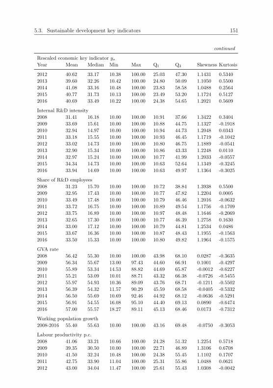
5.3. Sustainable development key indicators 151
continued
Rescaled economic key indicator ysYear Mean Median Min Max Q1 Q3 Skewness Kurtosis
2012 40.62 33.17 10.38 100.00 25.03 47.30 1.1431 0.5340
2013 39.60 32.26 10.42 100.00 24.80 50.09 1.1050 0.5500
2014 41.08 33.16 10.48 100.00 23.83 58.58 1.0488 0.2564
2015 40.77 31.73 10.13 100.00 23.49 53.20 1.1724 0.5127
2016 40.69 33.49 10.22 100.00 24.38 54.65 1.2021 0.5609
Internal R&D intensity
2008 31.41 16.18 10.00 100.00 10.91 37.66 1.3422 0.3404
2009 33.69 15.61 10.00 100.00 10.88 44.75 1.1327 -0.1918
2010 32.94 14.97 10.00 100.00 10.94 44.73 1.2048 0.0343
2011 33.18 15.55 10.00 100.00 10.93 46.45 1.1719 -0.1042
2012 33.02 14.73 10.00 100.00 10.80 46.75 1.1889 -0.0541
2013 32.90 15.34 10.00 100.00 10.86 43.33 1.2248 0.0110
2014 32.97 15.24 10.00 100.00 10.77 41.99 1.2033 -0.0557
2015 34.34 14.73 10.00 100.00 10.63 52.64 1.1349 -0.3245
2016 33.94 14.69 10.00 100.00 10.63 49.97 1.1364 -0.3025
Share of R&D employees
2008 31.23 15.70 10.00 100.00 10.72 38.84 1.3938 0.5500
2009 32.95 17.43 10.00 100.00 10.77 47.82 1.2204 0.0005
2010 33.49 17.48 10.00 100.00 10.79 46.46 1.2016 -0.0632
2011 33.72 16.75 10.00 100.00 10.89 49.54 1.1756 -0.1709
2012 33.75 16.89 10.00 100.00 10.97 48.48 1.1646 -0.2069
2013 32.65 17.30 10.00 100.00 10.77 46.39 1.2758 0.1630
2014 33.00 17.12 10.00 100.00 10.79 44.81 1.2534 0.0486
2015 33.67 16.36 10.00 100.00 10.87 48.43 1.1955 -0.1563
2016 33.50 15.33 10.00 100.00 10.80 49.82 1.1964 -0.1575
GVA rate
2008 56.42 55.30 10.00 100.00 43.98 68.10 0.0287 -0.3635
2009 56.34 55.67 13.00 97.43 44.60 66.91 0.1001 -0.4297
2010 55.89 53.34 14.53 88.82 44.69 65.87 -0.0012 -0.6227
2011 55.21 53.09 10.01 88.71 43.32 66.38 -0.0726 -0.5455
2012 55.97 54.93 10.36 89.09 43.76 68.71 -0.1211 -0.5502
2013 56.39 54.32 11.57 90.29 45.59 68.58 -0.0405 -0.5332
2014 56.50 55.69 10.69 92.46 44.92 68.12 -0.0636 -0.5291
2015 56.91 54.55 16.08 95.10 44.40 69.13 0.0890 -0.6474
2016 57.00 55.57 18.27 89.11 45.13 68.46 0.0173 -0.7312
Working population growth
2008-2016 55.40 55.63 10.00 100.00 43.16 69.48 -0.0750 -0.3053
Labour productivity p.c.
2008 41.06 33.21 10.66 100.00 24.28 51.32 1.2254 0.5718
2009 39.35 30.50 10.00 100.00 22.71 46.89 1.3106 0.6708
2010 41.50 32.24 10.48 100.00 24.38 55.45 1.1102 0.1707
2011 42.75 33.90 11.04 100.00 25.31 55.86 1.0488 0.0621
2012 43.00 34.04 11.47 100.00 25.61 55.43 1.0308 -0.0042

152 Chapter 5. Empirical findings
continued
Rescaled economic key indicator ysYear Mean Median Min Max Q1 Q3 Skewness Kurtosis
2013 43.52 34.97 11.09 100.00 25.81 55.18 1.0563 0.0962
2014 44.67 35.95 11.67 100.00 27.31 57.81 0.9862 -0.0592
2015 46.63 37.58 12.57 100.00 28.92 62.84 0.8237 -0.5247
2016 47.58 39.13 12.83 100.00 28.80 62.76 0.7862 -0.6243
Labour productivity p.h.
2008 41.83 33.73 10.53 100.00 28.13 49.98 1.2922 1.1815
2009 40.96 33.67 10.00 100.00 27.85 54.82 1.3147 1.2922
2010 43.28 34.96 10.72 100.00 27.86 57.25 1.0695 0.3496
2011 44.45 34.97 11.78 100.00 28.04 54.88 1.0495 0.1819
2012 45.40 36.14 12.80 100.00 29.01 59.44 0.9821 0.0693
2013 46.41 38.31 12.77 100.00 31.08 60.12 1.0464 0.2055
2014 47.69 38.49 13.87 100.00 33.11 60.75 1.0312 0.0522
2015 49.00 39.99 15.05 100.00 33.86 61.79 0.9078 -0.2007
2016 50.44 40.83 15.67 100.00 33.89 63.33 0.8672 -0.3456
Net import intensity
2008 56.30 64.19 10.00 100.00 46.69 65.91 -0.3258 -0.8759
2009 56.77 65.04 10.00 100.00 48.76 66.45 -0.3748 -0.8862
2010 56.22 64.44 10.00 100.00 46.85 67.30 -0.3340 -0.8976
2011 58.06 64.89 10.00 100.00 53.62 69.09 -0.4384 -0.6789
2012 56.87 66.25 10.00 100.00 47.04 66.25 -0.3690 -0.7118
2013 55.75 63.76 10.00 100.00 36.23 74.75 -0.2481 -0.8921
2014 54.20 61.67 10.00 100.00 33.27 63.07 -0.1502 -0.8442
2015 53.86 61.67 10.00 100.00 26.10 61.67 -0.1184 -0.9193
2016 55.19 61.19 10.00 100.00 49.86 61.19 -0.2208 -0.7384
Share of imported input
2008 35.61 28.01 10.50 100.00 20.51 46.34 1.1876 0.7299
2009 34.38 27.35 10.37 100.00 19.58 44.90 1.3586 1.5468
2010 37.32 30.30 10.27 100.00 20.41 52.24 1.0514 0.5389
2011 37.71 29.62 10.00 100.00 20.91 52.58 1.0248 0.4422
2012 38.64 31.06 10.02 100.00 21.96 51.58 1.0007 0.3388
2013 38.65 29.78 12.70 100.00 22.16 53.06 1.0452 0.5051
2014 38.25 29.94 12.22 100.00 21.82 53.12 1.0649 0.5651
2015 39.06 29.49 12.20 100.00 22.21 55.41 0.9321 0.0487
2016 38.89 29.79 11.71 100.00 22.09 55.14 1.0423 0.3256
Table 5.13 Summary statistics of the rescaled economic key indicators in the German economyfrom 2008 to 2016; GVA, Gross Value Added; Max, Maximum; Min, Minimum;p.c., per capita; p.h., per hour; Q1, 25
th percentile; Q3, 75th percentile; R&D,
Research and Development
of the share of imported input are located below normal percentiles, such that the
distribution is heavily skewed to the right. Contributions to international trade (SDG
17.11) should be advanced.
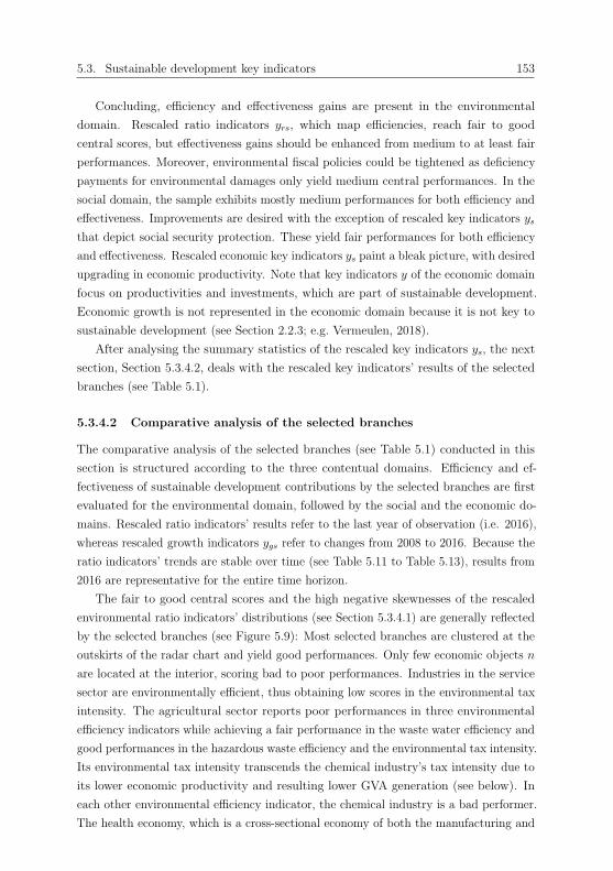
5.3. Sustainable development key indicators 153
Concluding, efficiency and effectiveness gains are present in the environmental
domain. Rescaled ratio indicators yrs, which map efficiencies, reach fair to good
central scores, but effectiveness gains should be enhanced from medium to at least fair
performances. Moreover, environmental fiscal policies could be tightened as deficiency
payments for environmental damages only yield medium central performances. In the
social domain, the sample exhibits mostly medium performances for both efficiency and
effectiveness. Improvements are desired with the exception of rescaled key indicators ys
that depict social security protection. These yield fair performances for both efficiency
and effectiveness. Rescaled economic key indicators ys paint a bleak picture, with desired
upgrading in economic productivity. Note that key indicators y of the economic domain
focus on productivities and investments, which are part of sustainable development.
Economic growth is not represented in the economic domain because it is not key to
sustainable development (see Section 2.2.3; e.g. Vermeulen, 2018).
After analysing the summary statistics of the rescaled key indicators ys, the next
section, Section 5.3.4.2, deals with the rescaled key indicators’ results of the selected
branches (see Table 5.1).
5.3.4.2 Comparative analysis of the selected branches
The comparative analysis of the selected branches (see Table 5.1) conducted in this
section is structured according to the three contentual domains. Efficiency and ef-
fectiveness of sustainable development contributions by the selected branches are first
evaluated for the environmental domain, followed by the social and the economic do-
mains. Rescaled ratio indicators’ results refer to the last year of observation (i.e. 2016),
whereas rescaled growth indicators ygs refer to changes from 2008 to 2016. Because the
ratio indicators’ trends are stable over time (see Table 5.11 to Table 5.13), results from
2016 are representative for the entire time horizon.
The fair to good central scores and the high negative skewnesses of the rescaled
environmental ratio indicators’ distributions (see Section 5.3.4.1) are generally reflected
by the selected branches (see Figure 5.9): Most selected branches are clustered at the
outskirts of the radar chart and yield good performances. Only few economic objects n
are located at the interior, scoring bad to poor performances. Industries in the service
sector are environmentally efficient, thus obtaining low scores in the environmental tax
intensity. The agricultural sector reports poor performances in three environmental
efficiency indicators while achieving a fair performance in the waste water efficiency and
good performances in the hazardous waste efficiency and the environmental tax intensity.
Its environmental tax intensity transcends the chemical industry’s tax intensity due to
its lower economic productivity and resulting lower GVA generation (see below). In
each other environmental efficiency indicator, the chemical industry is a bad performer.
The health economy, which is a cross-sectional economy of both the manufacturing and

154 Chapter 5. Empirical findings
0
20
40
60
80
100
Air emissions efficiency
Energy efficiency
Water efficiency
Waste water efficiency
Hazardous waste efficiency
Environmental tax intensity
●
●
●
●
●
●
●
●
●
●
●
●
●
●
Health economyAgricultural sectorManufacturing sectorChemical industryCar industryService sectorIT industryFinancial industryReal estate industryOverall German economy
Figure 5.9 Environmental ratio indicators in rescaled performance scores for the selectedbranches in the German economy in 2016; IT, Information Technology
the service sectors, is clustered along with the service sector’s selected branches. Its
stakes in the manufacturing sector are not concentrated on environmentally polluting
industries. For example, only 5.23% of the chemical industry is attributable to the
health economy in 2016 (see Appendix A.2).
The environmental growth indicators’ distributions are clustered approximately
between medium and fair performance scores (see Figure 5.10). Best displayed per-
formers are the financial industry in the reduction of air emissions (63.94 in 2016)
and primary energy consumption (67.60 in 2016) as well as the car industry in the
reduction of water use (65.83 in 2016) and waste water (65.06 in 2016). The IT industry
scores best among the selected branches in the reduction of hazardous waste (77.05 in
2016). However, the IT industry’s further outcomes are sparse. The chemical industry
neither scores with environmental efficiency (see Figure 5.9) nor with environmental
effectiveness: Its reduction rates are among the lowest, and only yield medium for the
reduction of air emissions (44.26 in 2016) and hazardous waste (42.51 in 2016). The
agricultural industry obtains consistent medium scores, with the exceptions of a fair
performance in the reduction of air emissions and a bad performance in the reduction
of hazardous waste. However, it achieves a good performance in the ratio indicator
hazardous waste efficiency (see Figure 5.9), and it may be concluded that a lack in the
reduction of hazardous waste is less harming.
Rescaled ratio indicators yrs of the social domain are rather distributed across
the scale, and performances of the selected branches range from bad to good (see
Figure 5.11). In contrast to the environmental domain, a segmentation of industries in

5.3. Sustainable development key indicators 155
0
20
40
60
80
100
Reduction of air emissions
Reduction of primary energy
consumption
Reduction of water use
Reduction of waste water
Reduction of hazardous
waste
●
●
●●
●
●
●
● ●
●
●
●
Health economyAgricultural sectorManufacturing sectorChemical industryCar industryService sectorIT industryFinancial industryReal estate industryOverall German economy
Figure 5.10 Environmental growth indicators in rescaled performance scores for the selectedbranches in the German economy; IT, Information Technology
the manufacturing and the service sectors is not observed. Positively outstanding is the
financial industry with regard to three tax indicators, average compensations of employ-
ees, labour share, and the share of non-marginally-employed employees, contributing
to approaching decent work for all (SDG 8.5). A further leading industry is the car
industry with highest results among the selected branches for the average compensations
of employees, share of non-marginally-employed employees, and the quota of severely-
disabled employees. Despite the high values in the average compensations of employees,
the car industry only performs medium in the labour share and could distribute more
income to its employees. Weaknesses of this industry are the quota of gender equality
and the VAT intensity. Contributions to inclusion and equal opportunities (SDG 10.2;
SDG 10.3; SDG 10.4) should be improved. The real estate industry’s performances are
diverse. It yields good performances in the gender equalities but bad performances in
the labour share and the share of non-marginally-employed employees, harming decent
work for all (SDG 8.5). The IT industry is a mid-ranging industry, which is neither
among the best nor among the worst performers. The health economy operates well
in the quota of gender equality of marginally-employed employees; fairly in the labour
share, share of non-marginally-employed employees and the quota of severely-disabled
employees; but it features medium performances in the average compensation of em-
ployees p.h., the quota of gender equality, and the share of apprentices. Its average
compensation of employees p.c. is only poor. Targets on social protection are managed
(SDG 1.3), but targets on decent work (SDG 8.5) are not succeeded in. The overall
German economy, which is typically located between the manufacturing and the service
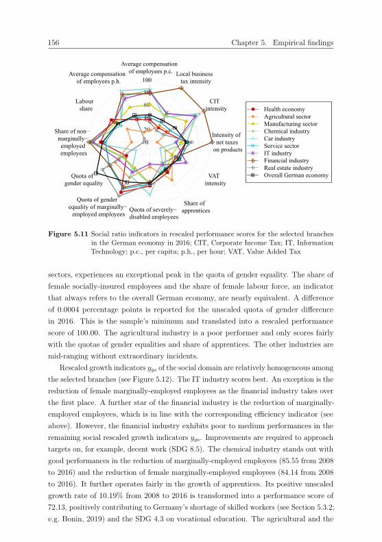
156 Chapter 5. Empirical findings
0
20
40
60
80
100
Average compensation of employees p.c.Average compensation
of employees p.h.
Labour share
Share of non− marginally− employed employees
Quota of gender equality
Quota of gender equality of marginally−
employed employees Quota of severely− disabled employees
Share of apprentices
VAT intensity
Intensity of net taxes
on products
CIT intensity
Local business tax intensity
●●●
●
●
●
●
●
●
●
●
●●
●
●●
●
●
●
●
●
●
●●
●
●
Health economyAgricultural sectorManufacturing sectorChemical industryCar industryService sectorIT industryFinancial industryReal estate industryOverall German economy
Figure 5.11 Social ratio indicators in rescaled performance scores for the selected branchesin the German economy in 2016; CIT, Corporate Income Tax; IT, InformationTechnology; p.c., per capita; p.h., per hour; VAT, Value Added Tax
sectors, experiences an exceptional peak in the quota of gender equality. The share of
female socially-insured employees and the share of female labour force, an indicator
that always refers to the overall German economy, are nearly equivalent. A difference
of 0.0004 percentage points is reported for the unscaled quota of gender difference
in 2016. This is the sample’s minimum and translated into a rescaled performance
score of 100.00. The agricultural industry is a poor performer and only scores fairly
with the quotas of gender equalities and share of apprentices. The other industries are
mid-ranging without extraordinary incidents.
Rescaled growth indicators ygs of the social domain are relatively homogeneous among
the selected branches (see Figure 5.12). The IT industry scores best. An exception is the
reduction of female marginally-employed employees as the financial industry takes over
the first place. A further star of the financial industry is the reduction of marginally-
employed employees, which is in line with the corresponding efficiency indicator (see
above). However, the financial industry exhibits poor to medium performances in the
remaining social rescaled growth indicators ygs. Improvements are required to approach
targets on, for example, decent work (SDG 8.5). The chemical industry stands out with
good performances in the reduction of marginally-employed employees (85.55 from 2008
to 2016) and the reduction of female marginally-employed employees (84.14 from 2008
to 2016). It further operates fairly in the growth of apprentices. Its positive unscaled
growth rate of 10.19% from 2008 to 2016 is transformed into a performance score of
72.13, positively contributing to Germany’s shortage of skilled workers (see Section 5.3.2;
e.g. Bonin, 2019) and the SDG 4.3 on vocational education. The agricultural and the

5.3. Sustainable development key indicators 157
0
20
40
60
80
100
Growth of compensation of employees
Growth of employees
Growth of socially−insured
employees
Reduction ofmarginally−employed
employees
Growth of female socially−insured
employees
Reduction of female marginally−employed
employees
Growth of severely−disabled
employees
Growth of apprentices
Growth of working population
●
●
●
●
●
●●
●
●
●
●
●
●
●
●
●
●
●
●
●
Health economyAgricultural sectorManufacturing sectorChemical industryCar industryService sectorIT industryFinancial industryReal estate industryOverall German economy
Figure 5.12 Social and economic growth indicators in rescaled performance scores for theselected branches in the German economy; IT, Information Technology
real estate industries are not able to strike with efficiencies but achieve mid-ranging
results in effectiveness.
Economic performances of the selected branches in the rescaled ratio indicators
yrs are displayed in Figure 5.13. In accordance with impressions from the summary
statistics (see Section 5.3.4.1), performances of the selected branches are skewed towards
the interior of the radar chart. However, the real estate industry stands out in five
economic rescaled ratio indicators yrs as the best performer among the selected branches.
It achieves good results in the degree of modernity, investment intensity, GVA rate, and
the labour productivities (p.c. and p.h.). It further stands out as the worst performer
among the selected branches in six economic rescaled ratio indicators yrs: the gross
capital productivity, net capital productivity, consumed capital productivity, internal
R&D intensity, share of R&D employees, and the share of imported input. Economic
productivity ought to be improved (SDG 8.2). The IT industry performs best in the
gross and the net capital productivity with further medium to good performances in
several economic rescaled ratio indicators yrs. The chemical and the car industries
yield similar performances with fair results in the rescaled ratio indicators yrs on R&D
and labour productivities. The agricultural sector’s economic performance remains
bad to medium, except for fair performances in the net import intensity. Economic
productivity (SDG 8.2) is not provided, but contributions to international trade (SDG
17.11) are realised. The manufacturing sector generally overshoots the service sector,
with the health and the overall German economies in its midst.
The economic domain’s only growth indicator – growth of working population – is

158 Chapter 5. Empirical findings
0
20
40
60
80
100
Gross capital productivityNet capital
productivity
Degree of modernity
Consumed capital
productivity
Investment intensity
Internal R&D intensity Share of
R&D employees
GVA rate
Labour productivity p.c.
Labour productivity
p.h.
Net import intensity
Share of imported input
●●
●
●
●
● ●
●
●
●
●
●
●●
●
●
●
●●
●
●
●
●
●
●
●
Health economyAgricultural sectorManufacturing sectorChemical industryCar industryService sectorIT industryFinancial industryReal estate industryOverall German economy
Figure 5.13 Economic ratio indicators in rescaled performance scores for the selected branchesin the German economy in 2016; GVA, Gross Value Added; IT, InformationTechnology; p.c., per capita; p.h., per hour; R&D, Research and Development
reported along with the social domain (see Figure 5.12) and yields similar results to
the social domain’s growth indicators ygs.
After scaling, weights ω are derived, and the diverse weighting methods’ results are
presented in the next section, Section 5.4.
5.4 Weighting
Three methods are applied to determine the MLSDI’s weights ω and importance
factors ψ: the PCA (see Section 4.3.7.2), PTA (see Section 4.3.7.3), and the MRMRB
algorithm (see Section 4.3.7.4). The PC family requires a priori analyses of eigenvalues
and explained cumulative variances to determine the included PCs. This is accomplished
in the first subsection of this section, Section 5.4.1. Section 5.4.2 outlines the MRMRB
algorithm’s diagnostics, and Section 5.4.3 compares and discusses the empirical findings
of the three weighting methods. The PC family further demands posteriori evaluations
of statistical test results, conducted in Section 5.4.4.
5.4.1 The Principal Component (PC) family’s eigenvalues and
explained cumulative variances
In the case of the PCA, PCs with eigenvalues larger than one are included (Kaiser’s
criterion), and at least 70% of the cumulative variance must be explained (see Sec-
tion 4.3.7.2; e.g. Field, 2009). The modified Kaiser’s criterion for the PTA requests
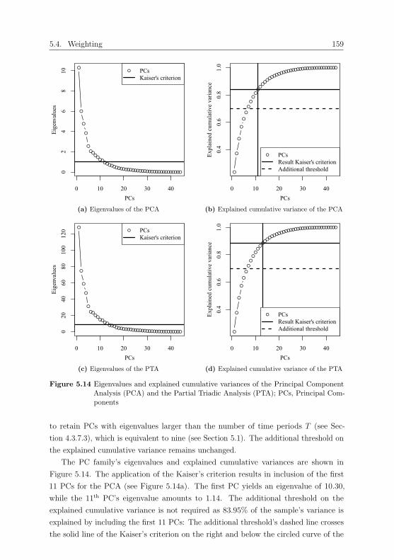
5.4. Weighting 159
●
●
●
●
●
●●●●
●●●●●●●●●●●●●●●●●●●●●●●●●●●●●●●●●●●
0 10 20 30 40
02
46
810
PCs
Eige
nval
ues
● PCsKaiser's criterion
(a) Eigenvalues of the PCA
●
●
●
●
●
●
●
●●
●●
●●
●●●●●●●●●●●●●●●●●●●●●●●●●●●●●●●
0 10 20 30 40
0.4
0.6
0.8
1.0
PCs
Expl
aine
d cu
mul
ativ
e va
rianc
e
● PCsResult Kaiser's criterionAdditional threshold
(b) Explained cumulative variance of the PCA
●
●
●
●
●
●●●●
●●●●●●●●●●●●●●●●●●●●●●●●●●●●●●●●●●●
0 10 20 30 40
020
4060
8010
012
0
PCs
Eige
nval
ues
● PCsKaiser's criterion
(c) Eigenvalues of the PTA
●
●
●
●
●
●
●
●●
●●
●●
●●●●●●●●●●●●●●●●●●●●●●●●●●●●●●●
0 10 20 30 40
0.4
0.6
0.8
1.0
PCs
Expl
aine
d cu
mul
ativ
e va
rianc
e
● PCsResult Kaiser's criterionAdditional threshold
(d) Explained cumulative variance of the PTA
Figure 5.14 Eigenvalues and explained cumulative variances of the Principal ComponentAnalysis (PCA) and the Partial Triadic Analysis (PTA); PCs, Principal Com-ponents
to retain PCs with eigenvalues larger than the number of time periods T (see Sec-
tion 4.3.7.3), which is equivalent to nine (see Section 5.1). The additional threshold on
the explained cumulative variance remains unchanged.
The PC family’s eigenvalues and explained cumulative variances are shown in
Figure 5.14. The application of the Kaiser’s criterion results in inclusion of the first
11 PCs for the PCA (see Figure 5.14a). The first PC yields an eigenvalue of 10.30,
while the 11th PC’s eigenvalue amounts to 1.14. The additional threshold on the
explained cumulative variance is not required as 83.95% of the sample’s variance is
explained by including the first 11 PCs: The additional threshold’s dashed line crosses
the solid line of the Kaiser’s criterion on the right and below the circled curve of the
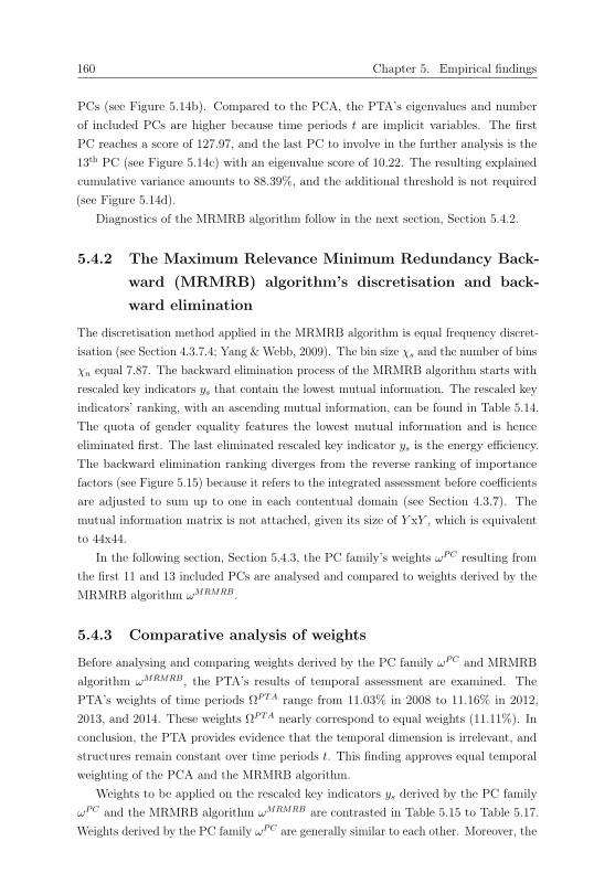
160 Chapter 5. Empirical findings
PCs (see Figure 5.14b). Compared to the PCA, the PTA’s eigenvalues and number
of included PCs are higher because time periods t are implicit variables. The first
PC reaches a score of 127.97, and the last PC to involve in the further analysis is the
13th PC (see Figure 5.14c) with an eigenvalue score of 10.22. The resulting explained
cumulative variance amounts to 88.39%, and the additional threshold is not required
(see Figure 5.14d).
Diagnostics of the MRMRB algorithm follow in the next section, Section 5.4.2.
5.4.2 The Maximum Relevance Minimum Redundancy Back-
ward (MRMRB) algorithm’s discretisation and back-
ward elimination
The discretisation method applied in the MRMRB algorithm is equal frequency discret-
isation (see Section 4.3.7.4; Yang & Webb, 2009). The bin size χs and the number of bins
χn equal 7.87. The backward elimination process of the MRMRB algorithm starts with
rescaled key indicators ys that contain the lowest mutual information. The rescaled key
indicators’ ranking, with an ascending mutual information, can be found in Table 5.14.
The quota of gender equality features the lowest mutual information and is hence
eliminated first. The last eliminated rescaled key indicator ys is the energy efficiency.
The backward elimination ranking diverges from the reverse ranking of importance
factors (see Figure 5.15) because it refers to the integrated assessment before coefficients
are adjusted to sum up to one in each contentual domain (see Section 4.3.7). The
mutual information matrix is not attached, given its size of Y xY , which is equivalent
to 44x44.
In the following section, Section 5.4.3, the PC family’s weights ωPC resulting from
the first 11 and 13 included PCs are analysed and compared to weights derived by the
MRMRB algorithm ωMRMRB.
5.4.3 Comparative analysis of weights
Before analysing and comparing weights derived by the PC family ωPC and MRMRB
algorithm ωMRMRB, the PTA’s results of temporal assessment are examined. The
PTA’s weights of time periods ΩPTA range from 11.03% in 2008 to 11.16% in 2012,
2013, and 2014. These weights ΩPTA nearly correspond to equal weights (11.11%). In
conclusion, the PTA provides evidence that the temporal dimension is irrelevant, and
structures remain constant over time periods t. This finding approves equal temporal
weighting of the PCA and the MRMRB algorithm.
Weights to be applied on the rescaled key indicators ys derived by the PC family
ωPC and the MRMRB algorithm ωMRMRB are contrasted in Table 5.15 to Table 5.17.
Weights derived by the PC family ωPC are generally similar to each other. Moreover, the

5.4. Weighting 161
Rank Rescaled key indicator ys Rank Rescaled key indicator ys
1 Quota of gender equality 23 Local business tax intensity
2 Share of apprentices 24 Environmental tax intensity
3 Intensity of net taxes on products 25 Reduction of marginally-employed em-ployees
4 Quota of gender equality ofmarginally-employed employees
26 Growth of female socially-insured em-ployees
5 Quota of severely-disabled employees 27 Hazardous waste efficiency
6 GVA rate 28 Labour productivity p.h.
7 Labour share 29 Consumed capital productivity
8 Degree of modernity 30 Growth of compensation of employees
9 Growth of apprentices 31 Investment intensity
10 VAT intensity 32 Air emissions efficiency
11 Share of non-marginally-employed em-ployees
33 Net import intensity
12 Reduction of air emissions 34 Average compensation of employeesp.h.
13 Reduction of primary energy consump-tion
35 Working population growth
14 Reduction of hazardous waste 36 Net capital productivity
15 Share of imported input 37 Water efficiency
16 Growth of severely-disabled employees 38 Waste water efficiency
17 Reduction of waste water 39 Internal R&D intensity
18 CIT intensity 40 Growth of employees
19 Reduction of female marginally-employed employees
41 Gross capital productivity
20 Labour productivity p.c. 42 Share of R&D employees
21 Reduction of water use 43 Growth of socially-insured employees
22 Average compensation of employeesp.c.
44 Energy efficiency
Table 5.14 Rescaled key indicators’ ranking according to the backward elimination of theMaximum Relevance Minimum Redundancy Backward (MRMRB) algorithm;CIT, Corporate Income Tax; GVA, Gross Value Added; p.c., per capita; p.h.,per hour; R&D, Research and Development; VAT, Value Added Tax
PC family’s weights ωPC remain close to equal weights. Equal weights would correspond
to values of 9.09% in the environmental domain, 5.00% in the social domain, and 7.69%
in the economic domain. Weights derived by the MRMRB algorithm ωMRMRB feature
higher variations.
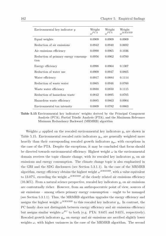
162 Chapter 5. Empirical findings
Environmental key indicator y WeightωPCA
WeightωPTA
WeightωMRMRB
Equal weights 0.0909 0.0909 0.0909
Reduction of air emissions 0.0942 0.0940 0.0692
Air emissions efficiency 0.0990 0.0965 0.1036
Reduction of primary energy consump-tion
0.0956 0.0962 0.0700
Energy efficiency 0.0998 0.0964 0.1307
Reduction of water use 0.0909 0.0947 0.0805
Water efficiency 0.0917 0.0884 0.1114
Reduction of waste water 0.0865 0.0946 0.0760
Waste water efficiency 0.0888 0.0850 0.1115
Reduction of hazardous waste 0.0842 0.0895 0.0705
Hazardous waste efficiency 0.0885 0.0863 0.0904
Environmental tax intensity 0.0809 0.0782 0.0863
Table 5.15 Environmental key indicators’ weights derived by the Principal ComponentAnalysis (PCA), Partial Triadic Analysis (PTA), and the Maximum RelevanceMinimum Redundancy Backward (MRMRB) algorithm
Weights ω applied on the rescaled environmental key indicators ys are shown in
Table 5.15. Environmental rescaled ratio indicators yrs are generally weighted more
heavily than their corresponding rescaled growth indicators ygs, with exceptions in
the case of the PTA. Despite the exceptions, it may be concluded that focus should
be directed towards environmental efficiency. Highest weight ω in the environmental
domain receives the topic climate change, with its rescaled key indicators ys on air
emissions and energy consumption. The climate change topic is also emphasised in
the GRI and the SDG disclosures (see Section 5.3.1.1). In the case of the MRMRB
algorithm, energy efficiency obtains the highest weight ωMRMRB, with a value equivalent
to 13.07%, exceeding the weight ωMRMRB of the closely related air emissions efficiency
(10.36%). From a natural science perspective, rescaled key indicators ys on air emissions
are contentually richer. However, from an anthropocentric point of view, sources of
air emissions – among others primary energy consumption – ought to be managed
(see Section 5.3.1.1). Thus, the MRMRB algorithm upgrades the energy efficiency and
assigns the highest weight ωMRMRB to this rescaled key indicator ys. In contrast, the
PC family does not distinguish between energy efficiency and air emissions efficiency
but assigns similar weights ωPC to both (e.g. PTA: 9.64% and 9.65%, respectively).
Rescaled growth indicators ygs on energy and air emissions are ascribed slightly lower
weights ω, with higher variances in the case of the MRMRB algorithm. The second
5.4. Weighting 163
most important environmental topic identified by the MRMRB algorithm is efficiency
of water use and waste water. The rescaled ratio indicators yrs on water obtain similar
weights by the MRMRB algorithm ωMRMRB (11.14% and 11.15%, respectively), but
the PC family allocates a higher weight ωPC to the water efficiency compared to the
waste water efficiency (e.g. PCA: 9.17% vs. 8.88%, respectively). These weights ωPC
are in line with the MRMRB algorithm’s result on rescaled ratio indicators yrs on
climate change: Rescaled key indicators ys that point towards the source of pollution
receive a higher weight ω. Relatively low weights ω are allocated to the hazardous
waste efficiency (e.g. MRMRB algorithm: 9.04%), despite the fact that it achieves best
central results among the rescaled key indicators ys of the environmental domain (see
Section 5.3.4.1). This finding demonstrates that weights’ magnitudes do not depend
on the empirical results of the rescaled key indicators ys but their interconnectedness,
reflecting synergies and trade-offs as desired (see Section 3.1; e.g. Costanza, Fioramonti
& Kubiszewski, 2016).
Regarding the social domain, rescaled growth indicators ygs receive higher weights
ω than their rescaled ratio indicators’ counterparts (see Table 5.16). Most important in
the social domain across the three weighting methods are the growth of socially-insured
employees and the growth of employees (e.g. MRMRB algorithm: 7.85% and 7.38%,
respectively). This finding is reasonable in two aspects: First, employment possesses
a dual purpose (source of income and key to transition; see Section 5.2.1; Harangozo
et al., 2018), and second, the key figure socially-insured employees is contentually richer
than the key figure employees because employees include decent as well as precarious
employment (see Section 5.2.1). A further interesting finding rests in the weighting of
the rescaled key indicators ys on compensations of employees. The average compensation
of employees p.h. receives a higher weight by the MRMRB algorithm ωMRMRB (6.89%)
than the average compensation of employees p.c. (5.36%). This is reasonable because the
latter rescaled key indicator ys is less precise, given its standardising key figure’s mixture
of full-time and part-time employees (see Section 5.2.1). Moreover, the labour share
receives the lowest weight ωMRMRB (4.02%) among the rescaled key indicators ys on
compensations of employees. From an employee’s perspective this finding is reasonable:
Not the proportion of the GVA distributed is of interest but the monetary value received
in relation to the work done. The PTA follows the MRMRB algorithm’s relation, but
the magnitude is nearly insignificant. In opposition, the PCA does not pursue this
relation but weights the labour share more heavily than the average compensation of
employees p.c. A further reasonable finding is the MRMRB algorithm’s higher (though,
nearly insignificant) weight ωMRMRB of the quota of gender equality of marginally-
employed employees and the quota of gender equality (3.51% and 3.17%, respectively).
At least two SDG targets are addressed with the first mentioned rescaled key indicator
ys – SDG 1.3 (social protection) and SDG 5.1 (end discrimination against women and
girls) – while the latter rescaled key indicator ys only addresses the SDG 1.3. The PCA
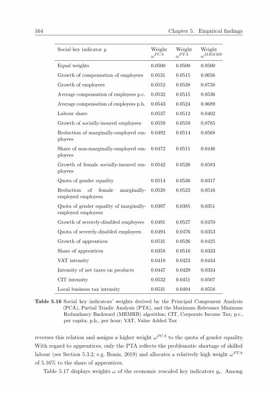
164 Chapter 5. Empirical findings
Social key indicator y WeightωPCA
WeightωPTA
WeightωMRMRB
Equal weights 0.0500 0.0500 0.0500
Growth of compensation of employees 0.0531 0.0515 0.0656
Growth of employees 0.0552 0.0538 0.0738
Average compensation of employees p.c. 0.0532 0.0515 0.0536
Average compensation of employees p.h. 0.0543 0.0524 0.0689
Labour share 0.0537 0.0512 0.0402
Growth of socially-insured employees 0.0559 0.0559 0.0785
Reduction of marginally-employed em-ployees
0.0492 0.0514 0.0568
Share of non-marginally-employed em-ployees
0.0472 0.0511 0.0446
Growth of female socially-insured em-ployees
0.0542 0.0526 0.0583
Quota of gender equality 0.0514 0.0536 0.0317
Reduction of female marginally-employed employees
0.0528 0.0523 0.0516
Quota of gender equality of marginally-employed employees
0.0397 0.0385 0.0351
Growth of severely-disabled employees 0.0491 0.0527 0.0470
Quota of severely-disabled employees 0.0494 0.0476 0.0353
Growth of apprentices 0.0531 0.0526 0.0425
Share of apprentices 0.0358 0.0516 0.0333
VAT intensity 0.0418 0.0423 0.0434
Intensity of net taxes on products 0.0447 0.0429 0.0334
CIT intensity 0.0532 0.0451 0.0507
Local business tax intensity 0.0531 0.0494 0.0558
Table 5.16 Social key indicators’ weights derived by the Principal Component Analysis(PCA), Partial Triadic Analysis (PTA), and the Maximum Relevance MinimumRedundancy Backward (MRMRB) algorithm; CIT, Corporate Income Tax; p.c.,per capita; p.h., per hour; VAT, Value Added Tax
reverses this relation and assigns a higher weight ωPCA to the quota of gender equality.
With regard to apprentices, only the PTA reflects the problematic shortage of skilled
labour (see Section 5.3.2; e.g. Bonin, 2019) and allocates a relatively high weight ωPTA
of 5.16% to the share of apprentices.
Table 5.17 displays weights ω of the economic rescaled key indicators ys. Among

5.4. Weighting 165
Economic key indicator y WeightωPCA
WeightωPTA
WeightωMRMRB
Equal weights 0.0769 0.0769 0.0769
Gross capital productivity 0.0862 0.0844 0.0940
Net capital productivity 0.0858 0.0843 0.0891
Degree of modernity 0.0692 0.0686 0.0518
Consumed capital productivity 0.0824 0.0825 0.0797
Investment intensity 0.0784 0.0763 0.0815
Internal R&D intensity 0.0840 0.0815 0.0907
Share of R&D employees 0.0820 0.0788 0.0961
GVA rate 0.0650 0.0650 0.0492
Working population growth 0.0776 0.0764 0.0885
Labour productivity p.c. 0.0852 0.0821 0.0646
Labour productivity p.h. 0.0785 0.0808 0.0729
Net import intensity 0.0596 0.0740 0.0842
Share of imported input 0.0661 0.0652 0.0578
Table 5.17 Economic key indicators’ weights derived by the Principal Component Analysis(PCA), Partial Triadic Analysis (PTA), and the Maximum Relevance MinimumRedundancy Backward (MRMRB) algorithm; GVA, Gross Value Added; p.c.,per capita; p.h., per hour; R&D, Research and Development
the rescaled ratio indicators yrs on capital, the gross capital productivity receives the
highest weight ω by all three weighting methods. This finding may be justified by
the fact that the gross capital productivity contains most information: It includes the
current value of assets as well as the depreciated value in relation to the generated GVA
(see Section 5.2.1; Section 5.3.1.3). The degree of modernity receives the lowest weight
ω among the capital indicators because it disregards the GVA, which is essential in
assessing economic productivity enhancements as of SDG 8.2. The GVA rate receives a
relatively low weight by the MRMRB algorithm ωMRMRB (4.92%). It does not indicate
productivity but merely value generation in proportion of the output (see Section 5.3.1.3).
The PC family does not recognise the GVA rate’s low explanatory power regarding
productivity and assigns weights ωPC of 6.50%. Similar to the average compensations
of employees, the labour productivities are weighted in an economically reasonable way
by the MRMRB algorithm: The rescaled key indicator p.h. receives a higher weight
ωMRMRB than its p.c. counterpart (7.29% vs. 6.46%, respectively). In contrast, the
PC family neglects this aspect and valorises the rescaled key indicator p.c. Last, the
MRMRB algorithm weights the net import intensity more heavily than the share of
imported input (8.42% vs. 5.78%, respectively). The net import intensity includes both

166 Chapter 5. Empirical findings
imports of input and imports for final consumption and is thus informationally richer.
The PTA follows this relation (however with a lower spread), but the PCA does not.
Weights ω indicate importances within a contentual domain but not towards the
overall MLSDI c1. The key indicators’ importance factors ψ towards the overall MLSDI
c1 are computed by adjusting weights ω with the rule of three (see Section 4.3.7).
Figure 5.15 portrays the importance factors ψ in a decreasing order according to the
MRMRB algorithm. Equal importance factors would correspond to values of 2.27%. In
view of the MRMRB algorithm, most important towards the overall MLSDI c1 are the
growth of socially-insured employees, growth of employees, and the energy efficiency.
Least important are the quota of gender equality, GVA rate, and the share of apprentices.
Ordering of the importance factors derived by the PC family ψPC differs from the
MRMRB algorithm’s ordering: Highest importance factors ψPC are assigned to the
gross capital productivity, growth of socially-insured employees, and the net capital
productivity. Because employment serves a dual mission (see Section 5.2.1; Harangozo
et al., 2018) and climate change is the main topic of the environmental domain (see
Section 5.3.1.1), the MRMRB algorithm’s ordering of importance factors ψMRMRB is
more plausible.
To sum up, the PC family does not clearly differentiate between diverse rescaled
key indicators ys, but weights ωPC are sticky around equal weights. The main aspects
of sustainable development are not captured. In contrast, the MRMRB algorithm
assigns higher weights ωMRMRB to informationally richer rescaled key indicators ys by
detecting higher order correlations. As a result, importance factors ψMRMRB towards
the overall MLSDI c1 correctly reflect most important topics of sustainable development.
In conclusion, the MRMRB algorithm outperforms the PC family, and the theoretical
superiority of the MRMRB algorithm (see Section 4.3.7.4) is supported by empirical
evidence. The MRMRB algorithm is the preferred and applied weighting method in
the further analysis. For the German sample, the MRMRB algorithm asserts to focus
efficiency in the environmental domain and effectiveness in the social domain.
Before applying weights derived by the MRMRB algorithm ωMRMRB on the rescaled
key indicators ys, statistical tests of the PC family are examined in the following section,
Section 5.4.4.
5.4.4 Statistical tests of the Principal Component (PC) family
Statistical tests of the PC family are conducted and analysed to verify the statistical
validity of the PC family’s results. Performed statistical tests include the KMO test
for sampling adequacy and the Bartlett’s test of sphericity (see Section 4.3.7.5; e.g.
Bartlett, 1950; Kaiser, 1970). To evaluate whether the tests should be based on Pearson’s
correlation coefficient for normal data or Kendall’s tau for non-normal data, normality of
z-score scaled key indicators yz are tested in the fashion of the key figures’ normality tests

5.4. Weighting 167
Quota of gender equalityGVA rate
Share of apprenticesIntensity of net taxes on products
Degree of modernityQuota of gender equality of marginally−employed employees
Quota of severely−disabled employeesShare of imported input
Reduction of air emissionsReduction of primary energy consumption
Reduction of hazardous wasteLabour share
Reduction of waste waterLabour productivity p.c.
Growth of apprenticesVAT intensity
Reduction of water useShare of non−marginally−employed employees
Growth of severely−disabled employeesLabour productivity p.h.
Environmental tax intensityHazardous waste efficiency
CIT intensityReduction of female marginally−employed employees
Consumed capital productivityInvestment intensity
Average compensation of employees p.c.Net import intensity
Local business tax intensityReduction of marginally−employed employees
Air emissions efficiencyWorking population growth
Net capital productivityGrowth of female socially−insured employees
Internal R&D intensityGross capital productivity
Water efficiencyWaste water efficiency
Share of R&D employeesGrowth of compensation of employees
Average compensation of employees p.h.Energy efficiency
Growth of employeesGrowth of socially−insured employees
Importance factors0.000 0.010 0.020 0.030
PCAPTAMRMRB
Figure 5.15 Importance factors of the Principal Component Analysis (PCA), Partial TriadicAnalysis (PTA), and the Maximum Relevance Minimum Redundancy Backward(MRMRB) algorithm; CIT, Corporate Income Tax; GVA, Gross Value Added;p.c., per capita; p.h., per hour; R&D, Research and Development; VAT, ValueAdded Tax
(see Section 4.3.3.4 and Section 5.2.2). The Shapiro-Wilk and the Kolmogorov-Smirnov
tests both conclude that 20 z-score scaled key indicators yz are normally distributed
and 14 z-score scaled key indicators yz are non-normal. Ambiguous results are obtained

168 Chapter 5. Empirical findings
for the remaining ten z-score scaled key indicators yz, with the following pattern: Data
are non-normal under the Shapiro-Wilk test but normal under the Kolmogorov-Smirnov
test. Therefore, histograms are consulted, but a clear decision cannot be made. The
test statistics and p-values are disclosed in Table A.12 to Table A.14, and two example
histograms of z-score scaled key indicators yz with ambiguous test results are provided
in Figure A.1 in the Appendix A.6. The average compensation of employees p.c. and
the consumed capital productivity experience the weakest and the strongest rejections
of the null hypotheses by the Shapiro-Wilk tests, respectively, with p-values of 0.04
and 0.0000, respectively. According to the multivariate Shapiro-Wilk test, the data are
multivariate non-normal, with a test statistic of 0.7483 and a p-value less or equal than
0.0001 (rejection of the null hypothesis). Given the ambiguities, the non-parametric
Kendall’s tau is preferred over the parametric Pearson’s coefficient for the KMO test of
sampling adequacy.
The KMO measure reveals the meritorious sampling adequacy of both the PCA
and the PTA with values amounting to 0.8370 (average from 2008 to 2016) and 0.8391,
respectively. The null hypotheses of the Bartlett’s tests are rejected in both cases with
p-values less or equal than 0.0001. The data are suitable for applying the PC family.
In conclusion, results of the PC family as of Section 5.4.3 remain valid.
The following section, Section 5.5, analyses the resulting subindices d and the overall
MLSDI c1 based on the MRMRB algorithm’s weights ωMRMRB.
5.5 Empirical findings of the four composite sus-
tainable development measures
The rescaled key indicators ys are weighted and geometrically aggregated to obtain the
subindices of each contentual domain d (see Section 4.3.8). The subindices d are then
aggregated into the overall MLSDI c1 via the geometric mean. Summary statistics of
the four composite measures are analysed in Section 5.5.1, and results of the selected
branches are evaluated in Section 5.5.2.
5.5.1 Summary statistics
The summary statistics of the subindices d mirror the impressions gained in the detailed
descriptions and analyses of the rescaled key indicators ys (see Section 5.3.4.1). Highest
scores in terms of the mean, median, maximum, and the 75th percentile are reached by
the environmental subindex (see Table 5.18). Its lead is followed by the social domain,
whereas the economic domain scores lowest.
The environmental subindex yields medium to fair central performances. Progress
over time is insignificant, but the distributional shape is in favour of environmental

5.5. Empirical findings of the four composite sustainable development measures 169
Composite measure
Year Mean Median Min Max Q1 Q3 Skewness Kurtosis
Environmental subindex
2008 55.19 61.04 12.61 82.86 41.91 69.80 -0.6895 -0.6591
2009 54.86 60.85 12.61 83.00 41.87 69.93 -0.6379 -0.7408
2010 55.22 61.31 12.61 82.65 42.12 69.87 -0.6775 -0.7207
2011 56.32 62.27 12.61 83.29 42.92 70.49 -0.7388 -0.6524
2012 56.27 61.99 12.61 82.93 42.70 70.08 -0.7648 -0.6346
2013 56.55 62.03 12.61 83.66 42.52 70.60 -0.7506 -0.6500
2014 56.83 63.01 12.61 83.87 42.64 70.51 -0.7727 -0.6090
2015 56.95 62.91 12.61 84.34 42.76 70.72 -0.7606 -0.6632
2016 57.16 63.33 12.61 84.40 42.90 70.78 -0.7604 -0.6782
Social subindex
2008 49.19 49.60 31.42 70.42 43.66 54.19 0.2653 -0.1445
2009 49.97 49.46 31.25 71.84 44.39 55.12 0.2807 -0.0123
2010 50.29 49.93 31.59 72.36 44.73 55.74 0.3624 0.0664
2011 51.19 50.52 34.80 72.76 45.74 55.88 0.3944 0.0219
2012 51.66 51.24 33.86 73.42 46.12 56.76 0.4416 0.1150
2013 51.98 51.63 33.77 73.88 45.99 57.40 0.3840 0.0409
2014 52.31 51.55 33.98 73.93 46.48 57.19 0.3986 0.0367
2015 52.48 52.19 34.54 74.16 46.82 57.49 0.4811 0.2606
2016 52.74 52.29 35.16 74.65 46.86 57.65 0.5000 0.2418
Economic subindex
2008 35.98 34.23 23.90 60.29 28.83 42.10 0.8642 -0.2037
2009 35.56 33.83 23.86 59.75 28.16 40.45 0.8844 -0.0433
2010 36.19 34.01 23.24 59.75 28.51 42.23 0.8258 -0.3054
2011 36.68 34.86 22.70 61.04 28.99 43.63 0.7793 -0.3650
2012 36.73 34.71 22.29 60.95 29.03 43.34 0.7658 -0.3882
2013 36.66 34.62 22.15 62.97 29.37 42.93 0.8159 -0.1276
2014 36.85 35.06 21.96 61.42 29.59 43.19 0.7642 -0.2943
2015 37.33 34.82 22.05 62.46 29.77 43.73 0.8390 -0.2724
2016 37.65 34.76 21.16 61.31 30.06 45.03 0.7827 -0.4680
Overall MLSDI c12008 45.16 45.71 30.78 62.33 39.70 50.48 -0.1574 -0.8220
2009 45.10 46.11 30.71 62.21 39.48 50.48 -0.1775 -0.7813
2010 45.58 46.88 30.97 62.86 39.68 51.41 -0.1570 -0.8301
2011 46.38 47.49 31.97 63.96 40.93 51.87 -0.1372 -0.8286
2012 46.50 47.63 31.68 64.34 41.09 51.98 -0.1618 -0.7792
2013 46.69 47.54 31.84 63.97 40.98 52.04 -0.1279 -0.8010
2014 46.96 47.73 32.37 64.03 42.27 52.12 -0.1343 -0.8289
2015 47.22 48.18 32.00 65.18 42.15 52.61 -0.1477 -0.8216
2016 47.49 48.54 31.60 65.20 42.44 53.10 -0.1301 -0.8264
Table 5.18 Summary statistics of the subindices and the overall Multilevel SustainableDevelopment Index (MLSDI) in the German economy from 2008 to 2016; Max,Maximum; Min, Minimum; Q1, 25
th percentile; Q3, 75th percentile

170 Chapter 5. Empirical findings
protection: The medians exceed the means, the 25th percentiles are located above a
score of 25.00, resulting in moderate negative skewnesses. Bottom performers should be
focused to enhance their performances, lifting the central measures to be at least fair.
Compared to the environmental subindex, the social subindex’s central performances
are weaker. A higher effort is required to yield fair performances. The social subindex’s
minima are the highest among the four composite measures’ minima. However, the
75th percentiles do not reach the fair bracket the normal score of 75.00 is located in.
Not the bottom but the centre of the distribution should be focused to improve social
development.
Among the three subindices d, the economic subindex performs worst. Its central
scores are rated as poor performances, and enhancements over time of the central meas-
ures, maxima, and the percentiles are insignificant. Additionally, minima deteriorate in
the course of time. The 25th percentiles just surpass the normal score of 25.00, and the
75th percentiles just reach the bracket of medium performances, remaining far from the
normal fair performances at scores of 75.00. Moderate positive skewnesses result, which
are undesirable distributional properties for economic prosperity. Major improvements
are required across the whole distribution.
The overall MLSDI’s distributional properties result from the subindices’ properties.
Central measures are located between the medium to fair performances of the environ-
mental subindex and the poor performances of the economic subindex. However, the
effect of the geometric aggregation comes to light. The overall MLSDI c1 is inclined
towards the poor economic performances: Its central measures only yield medium
performances at the lower end of the bracket, and the 75th percentiles do not yield the
normal 75.00.
The sample’s results of the four composite measures are illustrated in Figure 5.16
and Figure 5.17. Figure 5.16 contains the four composite measures’ performance
scores of the 62 economic objects n in the German economy from 2008 to 2016. The
environmental subindex features the highest spread, with relatively few economic objects
n at the bottom and relatively many economic objects n at the top of the distribution.
Compared, the social subindex’s spread is smaller, and especially the bottom of the
distribution is enhanced. The economic subindex features relatively many outcomes at
the bottom, and the overall MLSDI c1 overlaps the subindices d. Progress over time
has been made but should be enhanced for higher significance.
Figure 5.17 plots the four composite measures’ frequency distributions and densities,
strengthening the empirical findings of the previous analysis. The environmental
domain exhibits economic objects n with bad performances. These should be focused
for improvements. The social domain is not but should be represented at the top of the
distribution. Last, economic performances should be enhanced in their entirety.
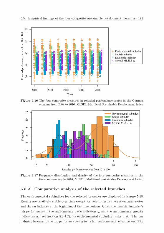
5.5. Empirical findings of the four composite sustainable development measures 171
2008 2010 2012 2014 2016
2040
6080
100
Years
Res
cale
d pe
rfor
man
ce sc
ores
from
10
to 1
00
● ● ● ● ● ● ●● ●
● ● ● ● ● ● ● ● ●●● ●
● ● ● ● ● ●
●● ●
●● ● ●
●●
● ● ● ● ● ● ● ● ●
●● ● ● ● ● ● ● ●
● ● ● ● ● ● ● ● ●● ● ● ● ● ● ● ● ●
● ● ● ● ● ● ● ● ●
●●
●
● ●●
●
● ●
● ● ● ● ● ● ● ● ●● ● ● ●
● ● ● ● ●
● ● ●● ● ● ● ● ●
● ● ● ● ● ● ● ● ●●
● ● ● ● ● ● ● ●●
● ● ● ● ● ● ● ●● ● ● ● ● ● ● ● ●● ● ● ● ● ●
● ● ●●
● ● ● ● ● ● ● ●
● ● ●● ● ●
● ● ●
● ● ●●
●● ●
●●
● ● ● ● ● ● ● ● ●
● ● ● ● ● ● ● ● ●● ● ●●
● ● ● ● ●
● ● ● ● ● ● ● ● ●
● ● ● ● ● ● ● ● ●
● ● ● ● ● ● ● ● ●● ● ● ● ● ● ● ● ●● ●
● ● ● ● ● ● ●
● ● ● ● ● ● ● ● ●
● ● ● ● ● ● ● ● ●
● ● ● ● ● ● ● ●●
● ●● ●
●● ● ● ●
● ● ● ● ● ● ● ● ●
● ● ● ● ● ● ●● ●
● ● ● ● ● ● ● ● ●● ● ● ● ● ●●
● ●● ● ● ● ●
● ● ● ●
● ● ●● ● ● ● ● ●
● ● ● ●● ● ● ● ●
● ● ● ● ● ● ● ● ●● ● ● ● ● ● ● ● ●
● ● ● ● ● ● ● ● ●
● ● ● ● ● ● ● ● ●
●●
● ●● ● ● ● ●
● ● ● ● ● ● ● ● ●
● ●● ● ● ● ● ● ●
●● ● ● ● ● ● ● ●
●● ●
● ● ● ● ● ●
● ● ● ● ● ● ● ● ●
● ● ● ● ● ● ● ● ●
● ●●
●● ● ● ● ●
● ● ●●
● ● ● ● ●
● ● ● ● ● ● ● ● ●● ● ● ● ● ● ● ● ●● ● ● ● ● ● ● ● ●
● ● ● ● ● ● ● ● ●● ● ● ● ● ● ● ● ●
● ● ●● ● ● ● ● ●
● ● ● ● ● ● ● ● ●●● ● ● ● ● ● ● ●
● ● ● ● ● ● ● ● ●
●
Environmental subindexSocial subindexEconomic subindexOverall MLSDI c1
Figure 5.16 The four composite measures in rescaled performance scores in the Germaneconomy from 2008 to 2016; MLSDI, Multilevel Sustainable Development Index
Rescaled performance scores from 10 to 100
Freq
uenc
y0
24
68
1012
10 20 40 60 80 100
Environmental subindexSocial subindexEconomic subindexOverall MLSDI c1
Figure 5.17 Frequency distribution and density of the four composite measures in theGerman economy in 2016; MLSDI, Multilevel Sustainable Development Index
5.5.2 Comparative analysis of the selected branches
The environmental subindices for the selected branches are displayed in Figure 5.18.
Results are relatively stable over time except for volatilities in the agricultural sector
and the car industry at the beginning of the time horizon. Given the financial industry’s
fair performances in the environmental ratio indicators yr and the environmental growth
indicators yg (see Section 5.3.4.2), its environmental subindex ranks first. The car
industry belongs to the top performers owing to its fair environmental effectiveness. The
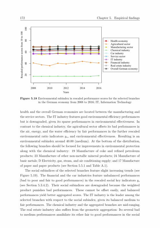
172 Chapter 5. Empirical findings
2008 2010 2012 2014 2016
2040
6080
100
Years
Res
cale
d pe
rfor
man
ce sc
ores
from
10
to 1
00
●● ●
● ●●
●● ●
● ● ● ● ● ● ● ● ●
●
●
Health economyAgricultural sectorManufacturing sectorChemical industryCar industryService sectorIT industryFinancial industryReal estate industryOverall German economy
Figure 5.18 Environmental subindex in rescaled performance scores for the selected branchesin the German economy from 2008 to 2016; IT, Information Technology
health and the overall German economies are located between the manufacturing and
the service sectors. The IT industry features good environmental efficiency performances
but is downgraded, given its sparse performances in environmental effectiveness. In
contrast to the chemical industry, the agricultural sector offsets its bad performances in
the air, energy, and the water efficiency by fair performances in the further rescaled
environmental ratio indicators yrs and environmental effectiveness. Resulting is an
environmental subindex around 40.00 (medium). At the bottom of the distribution,
the following branches should be focused for improvements in environmental protection
along with the chemical industry: 19 Manufacture of coke and refined petroleum
products; 23 Manufacture of other non-metallic mineral products; 24 Manufacture of
basic metals; D Electricity, gas, steam, and air conditioning supply; and 17 Manufacture
of paper and paper products (see Section 5.5.1 and Table A.1).
The social subindices of the selected branches feature slight increasing trends (see
Figure 5.19). The financial and the car industries feature unbalanced performances
(bad to poor and fair to good performances) in the rescaled social key indicators ys
(see Section 5.3.4.2). Their social subindices are downgraded because the weighted
product punishes bad performances. These cannot be offset easily, and balanced
performances yield better aggregated scores. The IT industry is the leader among the
selected branches with respect to the social subindex, given its balanced medium to
fair performances. The chemical industry and the aggregated branches are mid-ranging.
The real estate industry also suffers from the geometric aggregation: Its several bad
to medium performances annihilate its other fair to good performances in the social
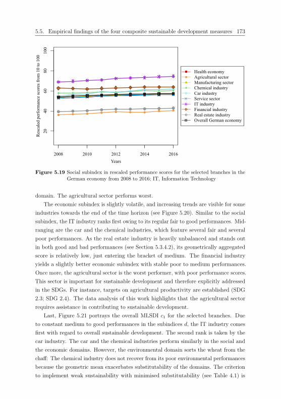
5.5. Empirical findings of the four composite sustainable development measures 173
2008 2010 2012 2014 2016
2040
6080
100
Years
Res
cale
d pe
rfor
man
ce sc
ores
from
10
to 1
00
● ● ● ● ● ● ● ● ●● ● ● ● ● ● ● ● ●
●
●
Health economyAgricultural sectorManufacturing sectorChemical industryCar industryService sectorIT industryFinancial industryReal estate industryOverall German economy
Figure 5.19 Social subindex in rescaled performance scores for the selected branches in theGerman economy from 2008 to 2016; IT, Information Technology
domain. The agricultural sector performs worst.
The economic subindex is slightly volatile, and increasing trends are visible for some
industries towards the end of the time horizon (see Figure 5.20). Similar to the social
subindex, the IT industry ranks first owing to its regular fair to good performances. Mid-
ranging are the car and the chemical industries, which feature several fair and several
poor performances. As the real estate industry is heavily unbalanced and stands out
in both good and bad performances (see Section 5.3.4.2), its geometrically aggregated
score is relatively low, just entering the bracket of medium. The financial industry
yields a slightly better economic subindex with stable poor to medium performances.
Once more, the agricultural sector is the worst performer, with poor performance scores.
This sector is important for sustainable development and therefore explicitly addressed
in the SDGs. For instance, targets on agricultural productivity are established (SDG
2.3; SDG 2.4). The data analysis of this work highlights that the agricultural sector
requires assistance in contributing to sustainable development.
Last, Figure 5.21 portrays the overall MLSDI c1 for the selected branches. Due
to constant medium to good performances in the subindices d, the IT industry comes
first with regard to overall sustainable development. The second rank is taken by the
car industry. The car and the chemical industries perform similarly in the social and
the economic domains. However, the environmental domain sorts the wheat from the
chaff: The chemical industry does not recover from its poor environmental performances
because the geometric mean exacerbates substitutability of the domains. The criterion
to implement weak sustainability with minimised substitutability (see Table 4.1) is

174 Chapter 5. Empirical findings
2008 2010 2012 2014 2016
2040
6080
100
Years
Res
cale
d pe
rfor
man
ce sc
ores
from
10
to 1
00
● ● ● ● ●● ● ● ●
● ● ● ● ● ● ● ● ●
●
●
Health economyAgricultural sectorManufacturing sectorChemical industryCar industryService sectorIT industryFinancial industryReal estate industryOverall German economy
Figure 5.20 Economic subindex in rescaled performance scores for the selected branches inthe German economy from 2008 to 2016; IT, Information Technology
2008 2010 2012 2014 2016
2040
6080
100
Years
Res
cale
d pe
rfor
man
ce sc
ores
from
10
to 1
00
● ● ●● ● ● ● ● ●
● ● ● ● ● ● ● ● ●
●
●
Health economyAgricultural sectorManufacturing sectorChemical industryCar industryService sectorIT industryFinancial industryReal estate industryOverall German economy
Figure 5.21 Overall Multilevel Sustainable Development Index (MLSDI) in rescaled per-formance scores for the selected branches in the German economy from 2008 to2016; IT, Information Technology
realised and comes into effect in aggregating the rescaled key indicators ys into the
subindices d (see above) and in aggregating the subindices d into the overall MLSDI c1.
The next section, Section 5.6, analyses the MLSDI’s sensitivities.

5.6. Sensitivity analyses 175
α = 1.5 vs.α = 3
α = 1.5 vs.α = ∞
α = 3.0 vs.α = ∞
PCA vs.PTA
PCA vs.MRMRB
PTA vs.MRMRB
Environmentalsubindex
2.9412 11.2647 9.6765 0.3824 1.7353 1.9706
Socialsubindex
2.5294 3.7941 1.8529 0.9118 1.9118 1.8529
Economicsubindex
2.5000 8.5588 7.4706 0.7353 1.7059 1.3824
OverallMLSDI c1
3.0882 9.4706 8.7059 0.9706 1.8824 2.0882
Table 5.19 Average rank shifts of economic objects by the four composite measures andthe three outlier and weighting methods in 2016; α, outlier coefficient; MLSDI,Multilevel Sustainable Development Index; MRMRB, Maximum Relevance Min-imum Redundancy Backward algorithm; PCA, Principal Component Analysis;PTA, Partial Triadic Analysis
5.6 Sensitivity analyses
Sensitivity analyses should be carried out for calculation steps with alternative ap-
proaches (see Section 4.3.9). These include missing value imputation (see Section 4.3.3
and Section 5.2.2), outlier detection (see Section 4.3.5 and Section 5.3.3), and weighting
(see Section 4.3.7 and Section 5.4). However, because Amelia II yields implausible
results (see Section 5.2.2), options for missing value imputation vanish. Hence, only
sensitivities of outlier detection and weighting are tested and analysed.
Average shifts in economic objects’ ranks by the four composite measures and the
three outlier detection methods are displayed in the first three columns of Table 5.19.
Full disclosure of the economic objects’ ranks by outlier coefficient α can be found in
Table A.15 in the Appendix A.7. As a result of a change of the outlier coefficient α from
1.5 to 3.0, economic objects n alter their ordinal rank position in the environmental
subindex on average by 2.94. With regard to the social and the economic subindices,
average rank shifts are slightly lower with values approximately equal to 2.50. Lower
outlier rates β in these two domains are responsible for this result. The average rank
shifts of the social and the economic subindices are approximately equal despite the fact
that the economic domain’s outlier rate β exceeds the social domain’s outlier rate β
(8.66% vs. 3.09%; see Section 5.3.3). This finding is explained by the differences in the
degree of outlyingness: The social domain involves strong outlying key indicators yo (e.g.
key indicators y on taxes; see Section 5.3.3) that are treated in both outlier treatment
cases (α = 1.5 and α = 3.0), whereas the economic domain features mixed outlying
key indicators yo (weak to strong; see Section 5.3.3) that are only treated partially in
the laxer case. The highest average rank shift is reported for the overall MLSDI c1
(3.09) because average rank shifts of the contentual domains enforce each other. When

176 Chapter 5. Empirical findings
2040
6080
100
Res
cale
d pe
rfor
man
ce sc
ores
from
10
to 1
00
● ● ●● ● ●
● ●●● ● ●
●●
●
● ●
●● ●
●
●●
●
● ●●
● ● ●
●●
●
●●
●●
●
●● ●●
● ●●
●●
●
● ●
●
●●
●
●●
●
●●
●
●●
●
●●
●●●
●
●●
●● ●●
●●
●●
●●
●●
●
●●
●
●●
●●
●●
● ●●
● ●●
●●
●● ●
●● ●●
● ●●
●●
●
● ●●
●
●
●● ●●
● ●
●
●●
●
●●
●
●●
●●
●
●
● ●●●
●●
●●
●● ●●
●●
●
● ●●
●●
●● ●●● ● ●
● ●●●
●●
●●
●●
● ●
● ●●
●●
●● ●●
α =
1.5
α =
3α
= ∞
α =
1.5
α =
3α
= ∞
α =
1.5
α =
3α
= ∞
α =
1.5
α =
3α
= ∞
●
Environmental subindexSocial subindexEconomic subindexOverall MLSDI
Figure 5.22 The four composite measures by the three outlier detection methods in res-caled performance scores in the German economy in 2016; MLSDI, MultilevelSustainable Development Index
comparing both outlier detection cases to the non-treatment case, average rank shifts
increase. The increases in rank shifts are in line with the outlier rates β because in
the non-treatment case, outlying key indicators yo are not treated at all irrespective
of the degree of outlyingness. The maximum average rank shift is reported by the
environmental subindex and detection at the inner fence vs. the non-treatment case.
Generally, average rank shifts of this case exceed average rank shifts of the detection at
the outer fence vs. the non-treatment case because detection at the outer fence is laxer,
such that fewer key indicators y are classified as outlying key indicators yo.
Figure 5.22 displays the sample’s four composite measures by the three outlier
detection methods. First, distributional differences are remarkable for the subindices d
that feature relatively high outlier rates β. These are the environmental and economic
subindices. In the non-treatment case, the economic objects n are closely clustered, and
the distributions feature low spreads. In the environmental domain, the distribution is
clustered at the top because strong outlying key indicators yo exist at the bottom (see e.g.
Figure 5.7b52). As a result of removing these, scales of the key indicators y are shortened,
such that more economic objects n feature bad or poor performances in the key indicators
y. As a result, these economic objects’ environmental subindices are downgraded towards
the lower end of the distribution. In the economic domain, the opposite occurs: In the
wake of outlier treatment, the distribution spreads towards the top because outlying
52Because of the air emissions intensity’s negative effective direction ξ−, the portrayed outlying keyindicators yo at the top constitute outlying key indicators yo at the bottom in view of the compositemeasures.

5.6. Sensitivity analyses 177
2040
6080
100
Res
cale
d pe
rfor
man
ce sc
ores
from
10
to 1
00
● ● ●● ● ●
● ● ●
● ● ●
● ● ●● ●●
● ● ●
● ● ●
● ●●
● ● ●
● ● ●
● ● ●
● ● ●
● ● ●● ● ●
● ● ●● ● ●● ● ●● ● ●● ●
●● ●
●● ● ●
● ● ●
● ● ●
● ●●
● ● ●
● ● ●● ● ●
● ● ●● ● ●● ● ●
● ● ●
● ● ●
● ● ●
● ● ●● ● ●
● ● ●
● ● ●
● ●●
● ●●
● ● ●● ● ●
● ● ●
● ● ●
● ● ●
● ●●
● ● ●● ● ●
● ● ●
● ● ●
● ● ●
● ● ●● ● ●
● ●●
● ● ●
● ● ●● ● ●● ● ●● ● ●
● ● ●
● ●●
● ● ●
PCA
PTA
MR
MR
B
PCA
PTA
MR
MR
B
PCA
PTA
MR
MR
B
PCA
PTA
MR
MR
B
●
Environmental subindexSocial subindexEconomic subindexOverall MLSDI c1
Figure 5.23 The four composite measures by the three weighting methods in rescaled perform-ance scores in the German economy in 2016; MLSDI, Multilevel SustainableDevelopment Index; MRMRB, Maximum Relevance Minimum RedundancyBackward algorithm; PCA, Principal Component Analysis; PTA, Partial Tri-adic Analysis
key indicators yo rather exist at the top (see e.g. Figure 5.8b). Second, variations in
the outlier coefficient α only result in significant changes in the economic domain. This
domain is the only domain with numerous weak to moderate outlying key indicators yo.
These are not detected in the laxer detection case. Sensitivities of the outlier detection
method of the sample’s full frequency distributions can be found in Figure A.2 in the
Appendix A.7.
Average rank shifts as a result of a change in the weighting method range from
0.3824 to 2.09 (see Table 5.19). The four composite measures are relatively robust
against changes in the weighting method. Average rank shifts of the PC family remain
below 1.00: On average, economic objects n change their ranks of the four composite
measures below one position. This finding is in line with the PC family’s similar weights
ωPC (see Section 5.4.3). Changing the weighting method from the PC family to the
MRMRB algorithm yields slightly higher average rank shifts. A complete report of
the economic objects’ ranks by the four composite measures and the three weighting
methods is provided in Table A.16 in the Appendix A.7.
Figure 5.23 illustrates the sample’s distributional changes as a result of the different
weighting methods, endorsing the average rank shifts’ finding: The four composite
measures’ distributions are relatively stable and robust to alterations in the weighting
method. Full frequency distributions of the sample by the four composite measures and
the three weighting methods can be found in Figure A.3 in the Appendix A.7.

178 Chapter 5. Empirical findings
In conclusion, economic objects’ rankings and performance scores are sensitive to
outlier detection but not to weighting. Outlier treatment distorts the true picture (see
Section 4.3.5.1; McGregor & Pouw, 2017) but is desired to remove statistical biases.
Outlier treatment should be accomplished in order to shorten scales and dissolve the
closely clustered economic objects n. Differentiation between economic objects n is
enabled, which is required to direct actions for improvement in sustainable development.
Especially the environmental domain profits from distortion of the true picture because
observations are lowered towards the bottom. Economic objects n at the bottom should
be focused for improved environmental protection. The strictness of the outlier detection
method only has an impact if weak to moderate outlying key indicators yo are present.
This is especially the case in the economic domain. To also reduce statistical bias in
this domain, the stricter base case (α = 1.5) is preferred. Furthermore, the superior
MRMRB algorithm remains to be recommended for weighting.
5.7 Summary
In this chapter, the novel methodology of the MLSDI has been deployed to the sample
region Germany. 62 branches of the German economy as well as five aggregated branches,
including the cross-sectional health economy, constitute the objects of investigation.
The time horizon reaches from 2008 to 2016. Sustainable development key figures
are collected from statistical authorities, and missing values are imputed by single
time series imputation. The sophisticated multiple panel data imputation algorithm
Amelia II fails because the normality assumption is violated. Missing values are
filled by single time series imputation. 44 sustainable development key indicators
are derived by aligning the meso GRI and the macro SDG frameworks, establishing
multilevel comparability of the MLSDI and finally addressing the perspective gap
empirically. Outliers are treated by the IQR method and are especially strong in the
environmental domain. Weights are derived by the PCA, PTA, and the MRMRB
algorithm. The theoretical advantage of the MRMRB algorithm to capture higher order
correlations is confirmed by the empirical findings: The MRMRB algorithm weights
informationally richer indicators more heavily, while the PC family does not establish
this clear pattern. Environmental efficiency indicators on climate change and social
effectiveness indicators on employment receive highest weights and should be focused
for improvements in sustainable development performances. The application of the
geometric aggregation achieves the desired effect of weak sustainability with minimised
substitutability: Bad performances are punished and cannot be easily compensated.
In conclusion, industries with unbalanced performances lag industries with rather
balanced results. The comparative analysis of the selected branches demonstrates
their contributions to sustainable development. The IT industry contributes most,
while improvements in the chemical industry’s environmental performance and the

5.7. Summary 179
agricultural industry’s performance with respect to all domains are required. The
agricultural industry’s importance for sustainable development is highlighted in the
SDGs and thus, actions and aid are urgently needed. Generally, the environmental
domain yields the highest central outcomes, while the economic domain yields the lowest
results. The environmental domain requires improvements in its bottom performers,
whereas the economic domain demands enhancements across the whole distribution.
The sensitivity analyses on outlier detection and weighting confirm the previously
derived results.

180 Chapter 5. Empirical findings
Open Access This chapter is licensed under the terms of the Creative Commons At -tribution 4.0 International License (http://creativecommons.org/licenses/by/4.0/), which permits use, sharing, adaptation, distribution and reproduction in any medium or format, as long as you give appropriate credit to the original author(s) and the source, provide a link to the Creative Commons license and indicate if changes were made.
The images or other third party material in this chapter are included in the chapter’s Creative Commons license, unless indicated otherwise in a credit line to the mate-rial. If material is not included in the chapter’s Creative Commons license and your intended use is not permitted by statutory regulation or exceeds the permitted use, you will need to obtain permission directly from the copyright holder.

Chapter 6
Discussion and conclusion
This chapter discusses and reflects on the accomplished theoretical (see Chapter 2
and Chapter 3), methodological (see Chapter 4), and the empirical research (see
Chapter 5). The present work is part of Phase C of the transdisciplinary research
agenda in sustainability science (see Section 2.3.4; e.g. Lang et al., 2012). It draws on
previous studies and problem framings from research and practice (Phase A), makes
use of prior disclosures from the scientific and the practitioner community (Phase B),
and finally provides new results that are relevant for both research and practice (Phase
C). Implications of the results for research, which bear on the descriptive-analytical
mode of sustainable development, are discussed in Section 6.1. Section 6.2 provides
implications for practice, which relate to the transformational mode outside the science
community (see Section 2.1; Wiek et al., 2012). Section 6.3 discusses limitations of the
present study, unfolding opportunities for future research. This dissertation ends with
an overall summary and conclusion in Section 6.4.
6.1 Implications for research
This work contributes to the debate on measurement and assessment of sustainable
development performances. In particular, it contributes a novel sustainable development
indicator set that includes a composite measure. Five related research gaps have been
identified: the perspective, operational-to-normative, knowledge, and the sustainab-
ility gaps as well as methodological deficiencies of existing sustainable development
indices. On the one hand, sustainable development demands multiple perspectives (see
Section 2.3.1; e.g. Lock & Seele, 2017) because the macro SDGs can only be achieved
if micro and meso objects contribute (see Section 2.3.1 and Section 2.3.2; e.g. Dahl,
2012; Griggs et al., 2014; T. Hahn et al., 2015). However, multiple perspectives are
frequently disregarded outside the sustainability transitions literature, constituting
the perspective gap. This work is the first to include the multilevel perspective in a
conceptual framework of sustainable development (see Section 2.3.1; Rotmans et al.,
© The Author(s) 2021C. Lemke, Accounting and Statistical Analyses for SustainableDevelopment, Sustainable Management, Wertschöpfung undEffizienz, https://doi.org/10.1007/978-3-658-33246-4_6
182 Chapter 6. Discussion and conclusion
2001) and thereby updates existing frameworks (see Chapter 2; e.g. Chofreh & Goni,
2017). The perspective gap has been closed theoretically, and further contributions
result. First, this work is the first to review sustainable development assessment meth-
ods by a method’s level of applicability (i.e. by the aggregational size of an object
of investigation; see Figure 3.1). This organisation is advantageous in further aspects
that are outlined in Section 6.2. Second, resulting from this review and based on the
sustainable development assessment principles, this work is the first to identify the
most suitable multilevel assessment method for comprehensive sustainable development
measurement. Indicator sets that include a composite measure have been revealed
as such a method. Third, this work contributes an advanced multilevel indicator set
that includes a composite measure and can be applied to meso and macro objects for
comparative analyses and benchmarking. The intersection of the meso GRI and the
macro SDG frameworks at target level as outlined in GRI and UNGC (2018a) has been
refined to indicator level and adjusted to current data availabilities for the German
economy by official statistics. On the other hand, decisions for sustainable development
should be made at operational, strategic, and normative tiers (see Section 2.3.2; e.g.
Ulrich, 2001). An operational-to-normative gap is present because decision makers
mostly address the operational tier only (see Section 2.3.2; e.g. Baumgartner & Rauter,
2017). Including the St. Gallen management model in the conceptual framework also
points towards indicator sets that include a composite measure as the most successful
tool in comprehensive multilevel measurement of sustainable development performances:
Indicators and indices address the operational and the strategic tiers (see Section 3.2;
e.g. Baumgartner, 2014) while being inherently normative (see Section 3.2; e.g. Waas
et al., 2014).
The third identified research gap is the knowledge gap (see Section 2.3.3; e.g. Weitz et
al., 2018). By tackling this gap, this work contributes insights about the interconnections
of individual sustainable development elements. In doing so, this work is the first to
apply an entropy-based information-theoretic algorithm to compute a sustainable
development index. Indices in the field of environmental sustainable development that
apply methods of information theory include, e.g. Fath and Cabezas (2004); P. E. Meyer,
Kontos, Lafitte and Bontempi (2007); and Pawlowski, Fath, Mayer and Cabezas (2005).
These are based on the parametric Fisher information, but the non-parametric entropy
should be preferred (see Section 4.3.7.4). Entropy-based index approaches include,
e.g. Rajsekhar, Singh and Mishra (2015); Ulanowicz, Goerner, Lietaer and Gomez
(2009); and Y. Zhang, Yang and Li (2006). Furthermore, Nie, Lv and Gao (2017) apply
information-theoretic entropy and the multilevel perspective on technological change
(see Section 2.3.1; Geels, 2002) to develop an index for power system transitions. An
example of an entropy-based application in a broader context of sustainable development
includes Wang et al. (2015), who assess sustainable development capacities with an
entropy-based weighting coefficient. However, to the best of the author’s knowledge,
6.1. Implications for research 183
aggregated sustainable development performances have not been estimated by means of
information-theoretic entropy. The application of an information-theoretic algorithm to
tackle synergies and trade-offs of individual sustainable development elements constitutes
the major methodological contribution of this work. Moreover, this study is the first
to compare two multivariate statistical techniques – the PCA and the PTA – to an
information-theoretic approach. It is also the first to estimate the three weighting
methods’ sensitivities on four composite measures of sustainable development.
The fourth identified research gap – the sustainability gap – regards the bottleneck
of the science-practice linkage (see Section 2.3.4; e.g. Hall et al., 2017). The present work
contributes to this bottleneck by providing detailed information about its methodological
approach and data sources, such that the MLSDI can be re-built by interested change
agents. Furthermore, this work is the first to publish data on 44 sustainable development
key indicators, three subindices, and an overall sustainable development index for 62 two-
digit industries as well as five aggregated branches, including the cross-sectional health
economy, in the German economy from 2008 to 2016. Providing detailed information
about the methodological approach, data sources, and objective, macro-economic
benchmarks entails two advantages: First, it enhances decision usefulness across the
decisional tiers by identifying and improving relevant sustainable development key
indicators; and second, it encourages corporations and further objects of investigation
to compare their performances to the provided macro-economic benchmarks, preventing
greenwashing.
Fifth and last, previous sustainable development indices do not only lack compli-
ance with the conceptual framework (see Section 3.3 and above), but especially the
assessment principle methodological soundness is violated (see Section 4.2). Insufficient
data cleaning, weighting, aggregation, and a lack of sensitivity analyses are frequent
shortcomings. This work has overcome these deficits and contributes a methodologically
sound sustainable development index: The MLSDI imputes missing values and treats
outliers, establishing credibility, validity, and reliability of measurement; it applies a
sophisticated information-theoretic algorithm to objectively determine relevances and
interconnections of individual sustainable development elements; it obeys mathematical
aggregation rules for credibility, validity, and reliability; and it conducts sensitivity
analyses, proving the measurement’s robustness and confirming its previously claimed
credibility, validity, and reliability.
Compared to the reviewed sustainable development indices, the MLSDI is the only
index that can be deployed at multiple levels (see Table 4.5). Hence, it features a wider
scope than the previous indices. Because the reviewed indices are distinct in their
indicator bases and regional scopes, data results are not comparable, and the MLSDI
is only related to the previous indices in respect of its methodology. The MLSDI may
serve management decisions, national industry policy, and international affairs, whereas
single level indices only address one level of decision making. For example, the DJSI
184 Chapter 6. Discussion and conclusion
support corporate decision making, and the SSI assists international policy making by
comparing country performances. In comparison with indices of single domains (e.g.
the EPI; Esty & Emerson, 2018), the MLSDI supports decision making with regard to
all three contentual domains of sustainable development. The MLSDI is based on 44
key indicators and exceeds the number of indicators of five of the nine reviewed indices.
Previous indices with a narrower indicator base include the ICSD (Krajnc & Glavic,
2005), FEEM SI (e.g. Pinar et al., 2014), HSDI (e.g. Bravo, 2018), SDI (Bolcarova &
Kolosta, 2015), and the SSI (e.g. van de Kerk et al., 2014). Their number of indicators
range from four to 38 (HSDI vs. ICSD, respectively). In conclusion, the MLSDI
assists a broader range of essential topics in sustainable development performance
measurement. Moreover, decision making based on the MLSDI will be more accurate in
general because of its overall methodological soundness. Only one of the nine reviewed
indices – the MISD (e.g. Shaker, 2018) – eliminates statistical biases by sound missing
value imputation. Statistical biases that originate in outlying observations remain for
all nine previous indices. With regard to scaling, three of the nine reviewed indices –
the SDGI (e.g. Schmidt-Traub et al., 2017a), SSI, and the WI (Prescott-Allen, 2001) –
apply a scaling method that correctly interplays with the deployed aggregation method.
However, of these three indices, the SSI is the only index that implements geometric
aggregation, which is essential to map the desired weak sustainability with minimised
substitutability (see Section 2.2.4 and Table 4.1). Only one of the reviewed indices – the
SDI – deploys the required bottom-up statistical weighting. The SDI determines weights
by a PCA, a powerful tool that is used in further sustainable development indices (e.g.
Barrios & Komoto, 2006; T. Li, Zhang, Yuan, Liu & Fan, 2012) and adjacent fields of
quantitative investigations of sustainable development (e.g. Fernandez-Feijoo, Romero
& Ruiz, 2014; Hansmann, Mieg & Frischknecht, 2012; Wallis, 2006). Nonetheless,
the methodological and empirical analyses have shown that the information-theoretic
algorithm outperforms this multivariate statistical technique because both linear and
higher order correlations are detected. Among the reviewed indices, the MLSDI is the
only index that implements an information-theoretic algorithm (see above) and hence
contributes a major methodological advancement to the index literature in general.
Last, only three of the reviewed indices – the FEEM SI, SDGI, and the SSI – investigate
sensitivities. The MLSDI improves their sensitivity analyses by intending to investigate
three calculation steps instead of one or two steps only. However, testing sensitivities
of missing value imputation becomes superfluous, given the Amelia II’s failure (see
Section 5.2.2).
6.2 Implications for practice
The present work provides several implications for corporate and political practices on
sustainable development. This work encourages practitioners to always view sustainable

6.2. Implications for practice 185
development as one integrated crisis of environmental protection, social development,
and economic prosperity (see Section 2.2.4; WSSD, 2002). The economic domain is
hallmarked by the misconception that economic growth or profits are part of sustainable
development. This work reminds practitioners to eliminate this misconception (see
Section 2.2.3; e.g. Jackson, 2009; Vermeulen, 2018). The present study advises corporate
practitioners to follow societal instrumental finality (see Section 2.3.2; e.g. T. Hahn &
Figge, 2011) because not the long-term survival of the company (i.e. profits) is part of
corporate sustainability, but corporations should contribute to the society level concept
of sustainable development. In fact, their contributions are inevitable for achieving
the SDGs (see Section 2.3.1; e.g. Dahl, 2012; Griggs et al., 2014). Furthermore, this
work recommends politicians to abandon GDP (i.e. economic growth) as a measure
of societal wellbeing (see Section 3.3.3; Costanza, Fioramonti & Kubiszewski, 2016)
and replace it by the MLSDI, which alludes to progress comprehensively and soundly.
However, political will might be lacking to let up on GDP (Jesinghaus, 2018).
This work further provides practitioners with an updated compilation of sustainable
development assessment principles, which should be considered in any sustainable devel-
opment assessment. The present study also delivers an updated overview of sustainable
development methods. For practitioners, the provided overview by aggregational size
might be easier to follow than, for example, overviews that are structured by the method-
ological approach (see Section 3.2; e.g. Sala et al., 2015). Practitioners might be unaware
of the methods required for their problem setting, but they most likely know if they
want to appraise, among others, a product, corporation, or a policy. The evaluation of
sustainable development assessment methods by means of the assessment principles (see
Section 3.2) entails two implications for practice. First, this work delivers an understand-
ing of each method, and second, the present study encourages practitioners to implement
sustainable development indicator sets that include a composite measure if they aim to
comprehensively measure sustainable development performances by multilevel objects.
Moreover, the evaluations of assessment principle compliances (see Section 3.3) and
methodological approaches (see Section 4.2) of previous sustainable development indices
result in two implications for practice. First, this work informs practitioners about
existing alternatives of sustainable development indices. Second, the present study
serves practitioners information about “do’s” and “don’ts” in sustainable development
index construction with regard to both the conceptual and the methodological phase.
Concerning the methodology, this work discloses profound knowledge, such that the
MLSDI can be re-built (see Section 6.1). The probably most important methodological
aspect for corporations provided in this work might be the utilisation of GVA instead
of revenues, sales, or profits (see Section 4.3.4). By means of the derived effectiveness
and efficiency indicators, the present study supports practitioners to manage absolute
and relative decoupling of sustainable development influences and economic activity,
respectively. This is a major challenge for decision makers (see Section 3.2; Holden et al.,
186 Chapter 6. Discussion and conclusion
2014). Furthermore, this work promotes the implementation of paradox teleological
integration to practitioners. All indicators should be followed at the same time, even
if they are conflicting (see Section 2.3.2; e.g. T. Hahn & Figge, 2011). Moreover, this
study delivers an advanced alignment of the GRI and the SDG frameworks at indicator
level for the geographical region Germany. The indicator base is expected to be valid in
further European countries. It further invites corporations that seek to report their per-
formances on the macro SDGs to rely on this alignment. The provided alignment might
be especially useful for corporations that are not able to allocate sufficient resources to
report on the comprehensive option of the GRI framework but are not satisfied with
the sparse core option. This study suggests collecting 36 key figures, a number that
balances comprehensiveness and resources in practice. Further, this work encourages
practitioners who are interested in data beyond the selected branches or Germany to
take advantage of the benchmarking opportunities the MLSDI provides by enclosing
detailed empirical analyses and data sources to re-produce the sample. Last, this work
may support the action plan for financing green growth in the EU. First, the present
study contributes to Action 1 of this plan, which encompasses the establishment of a
unified classification system for sustainable activities, also termed “EU taxonomy” (EC,
2018). On the one hand, the derived conceptual framework (see Figure 2.11) may guide
the establishment of the “shared understanding of what ‘sustainable’ means” (EC, 2018).
On the other hand, the elaborated indicator set that is applicable to both the meso and
the macro levels may support determining the environmental and the social objectives
investors should aim for. Second and foremost, this work contributes to Action 5:
developing sustainability benchmarks. More transparent and sounder methodologies
of sustainable development indices are demanded in order to halt greenwashing (EC,
2018). The MLSDI and its well-researched and transparently exposed methodology (see
Chapter 4) is capable to serve exactly this purpose.
6.3 Limitations and future outlook
Several limitations remain and may be investigated in future research. The social domain
requires further conceptual development. The leading framework of the social boundaries
(see Section 2.2.2; e.g. Raworth, 2017) mostly applies to needs of the developing, not the
developed world. Because Maslow’s hierarchy of needs (e.g. Maslow, 1987) covers needs
of both developing and developed countries, an alignment of the social boundaries and
Maslow’s hierarchy of needs might be expedient (see Section 2.2.2). Further research
on the concept of needs and possible harmonisations should be carried out. Similar to
the concept of the planetary boundaries (see Section 2.2.1; e.g. Steffen et al., 2015), the
finalised framework of social boundaries should be able to verify an indicator’s relevance
towards sustainable development (see Section 5.3.1.1 and Section 5.3.1.2).
The consideration of multiple levels sacrifices detailed analysis within one level.
6.3. Limitations and future outlook 187
In contrast to footprints, indicator sets typically report sustainable development per-
formances of one object of investigation while disregarding upstream or downstream
sustainable development performances. To deliver a holistic picture of the supply
chain, the MLSDI should be combined with footprint analyses: A multilevel sustainable
development footprint should be derived in future research. A combination of the
multilevel index with single level life cycle assessment, a powerful tool to quantify a
product’s sustainable development performance, for example, from “cradle to grave”
(see Section 3.2; Finnveden et al., 2009), might also spread interesting insights but
could be methodologically challenging. Topics such as economic proximity (e.g. Torre &
Zuindeau, 2009) are only reflected in the performance scores, and benefits that economic
objects may experience through proximity cannot be analysed in detail. The literature
review is limited by the definition of sustainable development indices, but indices that
are not included in the review might provide valuable methodological insights. Further
indices that apply information-theoretic weighting have been outlined in Section 6.1.
Moreover, the MLSDI’s methodology is subject to several limitations. Adjustments
of current prices of key figures reported in monetary units would increase methodological
soundness (see Section 4.3.1) because nine years of calculation are covered, and efficiency
indicators rely on both monetary and non-monetary units. An iterative algorithm on
the single missing value imputation that matches the aggregated branches would refine
the imputation results (see Section 4.3.3.2) and also enhance methodological soundness.
The multiple missing value imputation by the Amelia II algorithm might not only
fail because of the violation of the normality assumption, but because outliers are
still present (see Section 4.3.3.3 and Section 5.2.2). An iterative algorithm over the
calculation steps missing value imputation and outlier treatment could be tested. Only
one micro index – the BLI (see Section 3.3.3; OECD, 2017) – has been identified in the
literature, and the MLSDI’s key indicator base is currently limited to the alignment of
the meso GRI and the macro SDG frameworks (see Section 4.3.4). Further micro indices
and a micro framework should be developed. Literature to verify the GRI and the SDG
frameworks might unfold gaps and weaknesses in these reporting schemes. Conflicts
might be present (Spaiser et al., 2017), and the frameworks’ reflections of the planetary
and the social boundaries (i.e. the safe and just operating space) could be investigated.
Despite theoretical justifications, more sophisticated outlier detection and treatment
methods could be explored in future studies because the conducted sensitivity analyses
have revealed the importance of this calculation step. As the information-theoretic
algorithm outperformed established multivariate statistical methods for weighting,
information-theoretic outlier detection and treatment might be of interest. Further
information can be found in, e.g. Aggarwal (2017).
Probably the major limitation of the MLSDI is the applied internal scaling (see
Section 4.3.6.2). Targets and boundaries are excluded due to unavailable data. Results
depend on the distribution, and their significance is reduced. For example, there will

188 Chapter 6. Discussion and conclusion
still be well performing economic objects, if all objects feature a bad performance
(Dahl, 2018). Therefore, the safe and just operating space must be converted into lower
aggregational levels of corporations, industries, and nations expressed in terms of the
SDGs (Dahl, 2018; Schmidt-Traub et al., 2017a; Steffen et al., 2015). Research on this
breakdown only emerged recently and especially lacks the connection of the safe and just
operating space and the SDGs. The probably most relevant study is released by O’Neill
et al. (2018), who split up the planetary and the social boundaries into 150 nations.
Linkage of the planetary boundaries and the SDGs is not available as a peer-reviewed
contribution yet (Randers, Rockstrom & Stoknes, 2019), and literature regarding the
nexus of the social boundaries and the SDGs could not be identified. Other adjacent
studies, for example, design a framework for translating the planetary boundaries into
fair shares at national levels (Hayha, Lucas, van Vuuren, Cornell & Hoff, 2016), develop a
methodology to assess a country’s contribution to transgressing the planetary boundary
phosphorus (M. Li, Wiedmann & Hadjikakou, 2019), or investigate whether growth
has occurred within the planetary boundaries (i.e. genuine green growth) (Stoknes
& Rockstrom, 2018). Studies that deal with linking corporate sustainability and the
planetary boundaries include, e.g. Antonini and Larrinaga (2017); Dahlmann, Stubbs,
Griggs and Morrell (2019); Haffar and Searcy (2018); and Whiteman et al. (2013).
Nonetheless, to the best of the author’s knowledge, the safe and just operating space
has neither been disassembled to corporate nor to industry level yet. Consequently,
targets and boundaries could not be included in the German sample (nor in any other
geographical region). Methods and precise data generation at corporate, industry, and
national levels of the planetary and the social boundaries constitute a major future
field of research. The MLSDI connects to this new stream: Once the boundaries are
broken down, these data can be fed in the MLSDI to precisely quantify a meso object’s
contribution to the macro SDGs. Moreover, the boundaries’ scientific relationship must
be known and hence explored in future research for accurate weighting (see Section 4.3.7;
e.g. Ebert & Welsch, 2004; Steffen et al., 2015), making statistical weighting obsolete.
Furthermore, the three applied weighting methods (see Section 4.3.7) will never assign
zero weights because indicators that are not perfectly correlated always add variation to
the data set. The indicator selection and derivation process (see Section 4.3.4) cannot be
reverted. Weighting across the contentual domains currently fails, and the sum of weights
of one domain reflects the number of included key indicators. Subsequent adjustment is
accomplished (see Section 4.3.7), but the MLSDI remains biased towards efficiency. More
ratio than growth indicators are comprised without subsequent adjustments. Further
research is required to develop methods that implicitly account for unbalanced numbers
of indicators. The equal temporal weighting of the MRMRB algorithm is justified by the
PTA’s temporal weights (see Section 4.3.7.4 and Section 5.4.3). This procedure might
be inaccurate as the PC family is generally outperformed. Structures of the temporal
dimension could be investigated by information-theoretic applications in future studies.
6.3. Limitations and future outlook 189
To strengthen the MRMRB algorithm’s empirical results, sensitivities of discretisation
methods could be tested. Despite successful punishment of bad performances by the
geometric aggregation, the MLSDI is not capable of indicating urgency. This judgement
remains with decision makers and is hence subjective. Sensitivity analyses could be
advanced as OAT is generally criticised in the literature. More sophisticated methods
are available (Saltelli & Annoni, 2010; Saltelli et al., 2008).
The current sample is limited to meso-level and macro-level applications because
micro-level frameworks are not available. For a complete micro-to-macro connection,
micro frameworks must be developed, and macro boundaries must be downscaled to
lower aggregational levels (see above). To demonstrate the MLSDI’s capability of im-
plementing the multilevel perspective and highlighting the benchmarking opportunities
across aggregational levels, an empirical application to meso objects (i.e. corporations)
should be prospectively performed. Data sources are attached in the supplementary
material to facilitate future applications. Generally, the change agent group society is
underrepresented in the present sample. Business is involved by constituting the objects
of investigation, policy is reflected by the SDG framework, and science is included by the
investigation itself. Incorporating micro objects of investigation (i.e. individuals) would
solve these two limitations simultaneously. Moreover, the present indicator selection
exhibits several limitations. First, the inclusion of more indicators in the MLSDI is
desirable to cover all multilevel aspects of the SDGs, but further data are missing for
the German sample. Second, interpretability of existing indicators may be limited. For
example, the environmental tax intensity, which is the ratio of environmental taxes and
the GVA, rises if more environmental taxes are paid. On the one hand, the increase
affects sustainable development positively because pollution is paid up for. On the other
hand, more taxes are paid because more pollution is generated, harming sustainable
development. Effectiveness as well as efficiency of a taxation system remains subject to
further investigations (see Section 5.3.1.1). Regarding the social domain, the VAT’s
effective direction may also be questionable as the VAT is a non-progressive tax on an
economic object’s created value added. Financially well-placed economic objects are
equally burdened in nominal terms as economic objects in weaker financial positions.
The latter might suffer from financing social development. The key indicators on
apprentices might be limited in their explanatory power. The number of university
students may complete the picture on education, and data on labour market demands
by educational level is required to draw reliable conclusions on the effective directions
key indicators on education should carry. Indicators on trade also feature ambiguities.
First, trade’s effect on sustainable development may be ambiguous in general. Further
information on the contribution of trade to the SDGs can be found in, e.g. WTO (2018).
Second, Germany’s net import intensity might not indicate support for developing
countries. Products are mainly imported from the People’s Republic of China, the
Netherlands, France, United States of America, and Italy (descending order; Destatis,
190 Chapter 6. Discussion and conclusion
2019a). Only China is an economy in transition, while the other countries of origin
are developed countries (UN, 2019c). The poor to medium performances of the capital
indicators entail uncertain interpretations. Classically, a decrease in capital indicators
is interpreted negatively. However, in the digital era of big data and digitalisation,
economic prosperity might be possible to be achieved despite decapitalisation and
deinvestments – the IT industry stands out as the best performer (see Section 5.5.2).
Forward-looking scenarios as approached by, e.g. Carraro et al. (2013; see Sec-
tion 3.3.3) should be explored to develop future pathways for comprehensive multilevel
solutions by means of the MLSDI (see Section 2.2.4 and Section 2.3.4; e.g. Lang et al.,
2012; Leach et al., 2013). A forecast of six SDG indicators can be found in Joshi,
Hughes and Sisk (2015), and a review that provides assistance for national SDG scen-
ario modelling can be found in Allen, Metternicht and Wiedmann (2017). More research
is required in this field. The MLSDI’s current selection of key indicators focuses on
developed countries such as Germany. For instance, growth indicators of the economic
domain are disregarded because Germany is one of the major economies of the world
(see Section 5.3.1.3; UN, 2019c). However, the SDGs are universally applicable to all
countries (see Section 2.3.3; e.g. Glaser, 2012), inviting multinational applications and
country comparisons. In such applications, outlier thresholds, scales, and weights must
be homogeneous. To evaluate the usefulness of national vs. multinational calculations,
the MLSDI’s sample should be enlarged to explore both scopes.
Effectiveness of performance measurement by the MLSDI is not investigated in
the present work. Testa et al. (2018) find that greenwashing does not pay off (see
Chapter 3). However, more case studies on the use of sustainable development indicators
are required (Bell & Morse, 2018) to further evaluate the influence of sustainable
development indicator sets that include a composite measure on sustainable development
performance. Do such indicator systems only entail a bureaucratic burden, or do they
trigger improved sustainable development performances? Research on the nexus of
sustainable development indicators and sustainable development performances include,
e.g. Bond and Morrison-Saunders (2013); Bond et al. (2015); and Ramos and Caeiro
(2010), but further studies are needed. Additionally, future research should investigate
whether indicators or other tools should be mandatory and rather standardised in view
of effectiveness of measurement, supporting political decisions on reporting regulations.
Last, the usefulness of comprehensive, multilevel indicators and indices for managerial
and political decision making might be explored in future studies.
6.4 Summary and conclusion
In this dissertation, a methodological sound sustainable development index that is
applicable to the micro, meso, and the macro levels has been developed. Multilevel
assessment is crucial because the society level concept sustainable development can only

6.4. Summary and conclusion 191
be achieved if micro and meso objects contribute. Moreover, methodological soundness
is a prerequisite for serving as a credible, valid, and reliable basis for decision making.
First, this work has elaborated a conceptual framework and assessment principles
of sustainable development. Based on these, indicator sets that include a composite
measure have been proven to be most successful in comprehensively quantifying mul-
tilevel sustainable development performances. A new index – the MLSDI – has been
derived by linking the conceptual framework and the assessment principles to each index
calculation step. The empirical analysis has confirmed the accuracy and robustness
of the MLSDI’s methodology. For improved sustainable development, environmental
efficiency indicators on climate change and social effectiveness indicators on employment
as well as the chemical industry’s environmental performances and the agricultural
industry’s performances in all three contentual domains should be focused.
Manifold implications for research and practice follow from the conducted research.
This work is the first to contribute a methodologically sound multilevel indicator
set and a multilevel index (perspective gap) that address operational, strategic, and
normative tiers (operational-to-normative gap). It is also the first to deploy an entropy-
based, information-theoretic algorithm to examine interactions of individual sustainable
development elements (knowledge gap). This work provides unrestricted transparency
for replicability (sustainability gap), and the MLSDI serves a wide scope of managerial
and political decision-making purposes. An alignment of the meso GRI and the macro
SDG frameworks at indicator level is delivered for corporate practice, and politicians
are encouraged to replace GDP as a measure of wellbeing with the MLSDI.
In conclusion, the usefulness of the suggested approach for informed managerial and
political decision making is expected to be high from both theoretical and methodological
viewpoints but remains subject to further investigations at the micro, meso, and the
macro levels to succeed in the long-term goal and vision of sustainability.
192 Chapter 6. Discussion and conclusion
Open Access This chapter is licensed under the terms of the Creative Commons At -tribution 4.0 International License (http://creativecommons.org/licenses/by/4.0/), which permits use, sharing, adaptation, distribution and reproduction in any medium or format, as long as you give appropriate credit to the original author(s) and the source, provide a link to the Creative Commons license and indicate if changes were made.
The images or other third party material in this chapter are included in the chapter’s Creative Commons license, unless indicated otherwise in a credit line to the mate-rial. If material is not included in the chapter’s Creative Commons license and your intended use is not permitted by statutory regulation or exceeds the permitted use, you will need to obtain permission directly from the copyright holder.

Appendix
A.1 Statistical classification scheme of economic
activities in the European Union (EU)
Sectioncode
Divisioncode
Denotation
n/a n/a Health economy
A-U 01-99 Total German economy
A 01-03 Agriculture, forestry, and fishing
01 Crop and animal production, hunting and related service activities
02 Forestry and logging
03 Fishing and aquaculture
B 05-09 Mining and quarrying
C 10-33 Manufacturing
10-12 Manufacture of food products; manufacture of beverages; manufactureof tobacco products
13-15 Manufacture of textiles; manufacture of wearing apparel; manufacture ofleather and related products
16 Manufacture of wood and of products of wood and cork, except furniture;manufacture of articles of straw and plaiting materials
17 Manufacture of paper and paper products
18 Printing and reproduction of recorded media
19 Manufacture of coke and refined petroleum products
20 Manufacture of chemicals and chemical products
21 Manufacture of basic pharmaceutical products and pharmaceutical pre-parations
22 Manufacture of rubber and plastic products
23 Manufacture of other non-metallic mineral products
24 Manufacture of basic metals
© The Author(s) 2021C. Lemke, Accounting and Statistical Analyses for SustainableDevelopment, Sustainable Management, Wertschöpfung undEffizienz, https://doi.org/10.1007/978-3-658-33246-4

194 Appendix
continued
Sectioncode
Divisioncode
Denotation
25 Manufacture of fabricated metal products, except machinery and equip-ment
26 Manufacture of computer, electronic, and optical products
27 Manufacture of electrical equipment
28 Manufacture of machinery and equipment not elsewhere classified
29 Manufacture of motor vehicles, trailers, and semi-trailers
30 Manufacture of other transport equipment
31-32 Manufacture of furniture; other manufacturing
33 Repair and installation of machinery and equipment
D 35 Electricity, gas, steam, and air conditioning supply
E 36-39 Water supply; sewerage, waste management, and remediation activities
36 Water collection, treatment, and supply
37-39 Sewerage; waste collection, treatment, and disposal activities; materialsrecovery; remediation activities and other waste management services
F 41-43 Construction
G-S 45-96 Services
G 45-47 Wholesale and retail trade; repair of motor vehicles and motorcycles
45 Wholesale and retail trade, and repair of motor vehicles and motorcycles
46 Wholesale trade, except of motor vehicles and motorcycles
47 Retail trade, except of motor vehicles and motorcycles
H 49-53 Transportation and storage
49 Land transport and transport via pipelines
50 Water transport
51 Air transport
52 Warehousing and support activities for transportation
53 Postal and courier activities
I 55-56 Accommodation and food service activities
J 58-63 Information and communication
58 Publishing activities
59-60 Motion picture, video, and television programme production, soundrecording and music publishing activities; programming and broadcastingactivities
61 Telecommunications
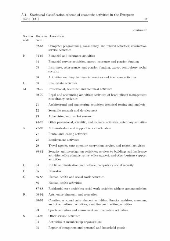
A.1. Statistical classification scheme of economic activities in the EuropeanUnion (EU) 195
continued
Sectioncode
Divisioncode
Denotation
62-63 Computer programming, consultancy, and related activities; informationservice activities
K 64-66 Financial and insurance activities
64 Financial service activities, except insurance and pension funding
65 Insurance, reinsurance, and pension funding, except compulsory socialsecurity
66 Activities auxiliary to financial services and insurance activities
L 68 Real estate activities
M 69-75 Professional, scientific, and technical activities
69-70 Legal and accounting activities; activities of head offices; managementconsultancy activities
71 Architectural and engineering activities; technical testing and analysis
72 Scientific research and development
73 Advertising and market research
74-75 Other professional, scientific, and technical activities; veterinary activities
N 77-82 Administrative and support service activities
77 Rental and leasing activities
78 Employment activities
79 Travel agency, tour operator reservation service, and related activities
80-82 Security and investigation activities; services to buildings and landscapeactivities; office administrative, office support, and other business supportactivities
O 84 Public administration and defence; compulsory social security
P 85 Education
Q 86-88 Human health and social work activities
86 Human health activities
87-88 Residential care activities; social work activities without accommodation
R 90-93 Arts, entertainment, and recreation
90-92 Creative, arts, and entertainment activities; libraries, archives, museums,and other cultural activities; gambling and betting activities
93 Sports activities and amusement and recreation activities
S 94-96 Other service activities
94 Activities of membership organisations
95 Repair of computers and personal and household goods
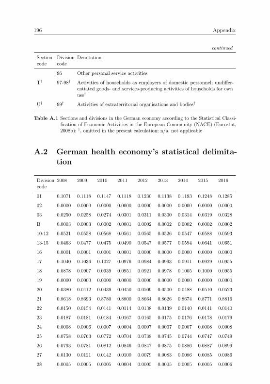
196 Appendix
continued
Sectioncode
Divisioncode
Denotation
96 Other personal service activities
T† 97-98† Activities of households as employers of domestic personnel; undiffer-entiated goods- and services-producing activities of households for ownuse†
U† 99† Activities of extraterritorial organisations and bodies†
Table A.1 Sections and divisions in the German economy according to the Statistical Classi-fication of Economic Activities in the European Community (NACE) (Eurostat,2008b); †, omitted in the present calculation; n/a, not applicable
A.2 German health economy’s statistical delimita-
tion
Divisioncode
2008 2009 2010 2011 2012 2013 2014 2015 2016
01 0.1071 0.1118 0.1147 0.1118 0.1230 0.1138 0.1193 0.1248 0.1285
02 0.0000 0.0000 0.0000 0.0000 0.0000 0.0000 0.0000 0.0000 0.0000
03 0.0250 0.0258 0.0274 0.0301 0.0311 0.0300 0.0314 0.0319 0.0328
B 0.0003 0.0003 0.0002 0.0001 0.0002 0.0002 0.0002 0.0002 0.0002
10-12 0.0521 0.0558 0.0568 0.0561 0.0565 0.0526 0.0547 0.0588 0.0593
13-15 0.0463 0.0477 0.0475 0.0490 0.0547 0.0577 0.0594 0.0641 0.0651
16 0.0001 0.0001 0.0001 0.0001 0.0000 0.0000 0.0000 0.0000 0.0000
17 0.1040 0.1036 0.1027 0.0976 0.0984 0.0993 0.0911 0.0929 0.0955
18 0.0878 0.0907 0.0939 0.0951 0.0921 0.0978 0.1005 0.1000 0.0955
19 0.0000 0.0000 0.0000 0.0000 0.0000 0.0000 0.0000 0.0000 0.0000
20 0.0380 0.0412 0.0439 0.0450 0.0509 0.0500 0.0488 0.0510 0.0523
21 0.8618 0.8693 0.8780 0.8800 0.8664 0.8626 0.8674 0.8771 0.8816
22 0.0150 0.0154 0.0141 0.0114 0.0138 0.0139 0.0140 0.0141 0.0140
23 0.0187 0.0181 0.0184 0.0167 0.0165 0.0175 0.0176 0.0178 0.0179
24 0.0008 0.0006 0.0007 0.0004 0.0007 0.0007 0.0007 0.0008 0.0008
25 0.0758 0.0763 0.0772 0.0704 0.0738 0.0745 0.0744 0.0747 0.0749
26 0.0793 0.0781 0.0812 0.0846 0.0847 0.0875 0.0886 0.0887 0.0899
27 0.0130 0.0121 0.0142 0.0100 0.0079 0.0083 0.0086 0.0085 0.0086
28 0.0005 0.0005 0.0005 0.0004 0.0005 0.0005 0.0005 0.0005 0.0006

A.2. German health economy’s statistical delimitation 197
continued
Divisioncode
2008 2009 2010 2011 2012 2013 2014 2015 2016
29 0.0000 0.0000 0.0000 0.0000 0.0000 0.0000 0.0000 0.0000 0.0000
30 0.0140 0.0145 0.0139 0.0149 0.0094 0.0103 0.0110 0.0124 0.0124
31-32 0.4077 0.4040 0.4084 0.4310 0.4221 0.4295 0.4317 0.4321 0.4328
33 0.0085 0.0078 0.0078 0.0079 0.0077 0.0078 0.0077 0.0081 0.0080
D 0.0004 0.0004 0.0004 0.0004 0.0003 0.0003 0.0003 0.0003 0.0003
36 0.0000 0.0000 0.0000 0.0000 0.0003 0.0003 0.0003 0.0003 0.0003
37-39 0.0001 0.0001 0.0001 0.0001 0.0001 0.0001 0.0001 0.0001 0.0001
F 0.0493 0.0513 0.0497 0.0461 0.0468 0.0466 0.0471 0.0474 0.0471
45 0.0000 0.0000 0.0000 0.0000 0.0000 0.0000 0.0000 0.0000 0.0000
46 0.1036 0.1052 0.1045 0.1061 0.1094 0.1102 0.1094 0.1113 0.1122
47 0.1445 0.1494 0.1493 0.1385 0.1443 0.1447 0.1470 0.1495 0.1511
49 0.0027 0.0029 0.0027 0.0029 0.0037 0.0039 0.0038 0.0040 0.0041
50 0.0000 0.0000 0.0000 0.0000 0.0000 0.0000 0.0000 0.0000 0.0000
51 0.0001 0.0001 0.0001 0.0000 0.0000 0.0000 0.0000 0.0000 0.0000
52 0.0000 0.0000 0.0000 0.0000 0.0000 0.0000 0.0000 0.0000 0.0000
53 0.0000 0.0000 0.0000 0.0000 0.0000 0.0000 0.0000 0.0000 0.0000
I 0.1089 0.1084 0.1061 0.1001 0.0999 0.0975 0.0958 0.0938 0.0936
58 0.1322 0.1362 0.1365 0.1240 0.1360 0.1462 0.1514 0.1517 0.1489
59-60 0.0003 0.0004 0.0004 0.0003 0.0003 0.0002 0.0002 0.0003 0.0003
61 0.0181 0.0188 0.0189 0.0193 0.0164 0.0175 0.0176 0.0178 0.0178
62-63 0.0329 0.0350 0.0336 0.0304 0.0332 0.0338 0.0332 0.0332 0.0334
64 0.0000 0.0000 0.0000 0.0000 0.0000 0.0000 0.0000 0.0000 0.0000
65 0.1351 0.1255 0.1407 0.1328 0.1285 0.1331 0.1193 0.1392 0.1248
66 0.0000 0.0000 0.0000 0.0000 0.0000 0.0000 0.0000 0.0000 0.0000
L 0.0097 0.0105 0.0102 0.0106 0.0097 0.0104 0.0106 0.0105 0.0106
69-70 0.0140 0.0143 0.0140 0.0129 0.0126 0.0139 0.0135 0.0139 0.0136
71 0.0230 0.0241 0.0232 0.0202 0.0196 0.0204 0.0206 0.0203 0.0201
72 0.1230 0.1215 0.1169 0.1243 0.1441 0.1494 0.1482 0.1431 0.1508
73 0.0532 0.0491 0.0448 0.0452 0.0464 0.0497 0.0470 0.0475 0.0456
74-75 0.0000 0.0000 0.0000 0.0000 0.0000 0.0000 0.0000 0.0000 0.0000
77 0.0197 0.0205 0.0198 0.0196 0.0255 0.0224 0.0224 0.0224 0.0224
78 0.0245 0.0244 0.0237 0.0272 0.0248 0.0272 0.0263 0.0263 0.0260

198 Appendix
continued
Divisioncode
2008 2009 2010 2011 2012 2013 2014 2015 2016
79 0.0354 0.0356 0.0351 0.0325 0.0312 0.0348 0.0340 0.0322 0.0323
80-82 0.0200 0.0211 0.0205 0.0209 0.0238 0.0253 0.0251 0.0249 0.0249
O 0.0593 0.0596 0.0609 0.0586 0.0589 0.0584 0.0579 0.0582 0.0596
P 0.0722 0.0654 0.0641 0.0636 0.0680 0.0658 0.0666 0.0672 0.0662
86 0.9990 0.9991 0.9990 0.9988 0.9988 0.9989 0.9987 0.9986 0.9987
87-88 0.6493 0.6521 0.6525 0.6393 0.6319 0.6427 0.6320 0.6398 0.6458
90-92 0.0000 0.0000 0.0000 0.0000 0.0000 0.0000 0.0000 0.0000 0.0000
93 0.5792 0.5775 0.5752 0.5799 0.5804 0.5841 0.5815 0.5807 0.5816
94 0.0191 0.0203 0.0200 0.0203 0.0253 0.0240 0.0241 0.0242 0.0239
95 0.0539 0.0564 0.0571 0.0570 0.0604 0.0675 0.0691 0.0671 0.0652
96 0.0119 0.0128 0.0127 0.0128 0.0142 0.0147 0.0151 0.0143 0.0150
Table A.2 German health economy’s stakes in divisions at two-digit level in percentage from2008 to 2016; see Table A.1 for denotation of section codes
A.3 Statistical tests of sustainable development key
figures
Environmental key figure x SWstatistic****
KSstatistic****
aDFstatistic**
LB stat-istic
LBp-values
Air emissions 0.2453 1.0000 -7.0959 0.0022 0.9624
Environmental tax 0.6172 1.0000 -7.9234 0.0014 0.9700
Hazardous waste 0.4722 0.9442 -8.0509 0.0012 0.9725
Primary energy consumption 0.3594 1.0000 -6.1263 0.0035 0.9528
Waste water 0.1728 0.8420 -8.5787 0.3866 0.5341
Water use 0.2258 0.8884 -8.3291 0.4063 0.5239
Table A.3 Environmental key figures’ test statistics and p-values of the Shapiro-Wilk (SW),Kolmogorov-Smirnov (KS), augmented Dickey-Fuller (aDF), and the Ljung-Box(LB) tests; **, p-values ≤ 0.01; ****, p-values ≤ 0.0001

A.3. Statistical tests of sustainable development key figures 199
Social key figure x SWstatistic****
KSstatistic****
aDFstatistic**
LB stat-istic
LBp-values
Apprentices 0.6837 1.0000 -9.0546 0.0061 0.9377
CIT 0.5082 0.5000 -8.5699 0.0003 0.9853
Compensation of employees 0.7636 0.8981 -8.5447 0.0001 0.9918
Employees 0.7473 0.9987 -8.4599 0.0003 0.9852
Female marginally-employed em-ployees
0.5427 1.0000 -6.8606 0.1399 0.7084
Female socially-insured employees 0.5749 1.0000 -8.5962 0.0003 0.9871
Local business tax 0.6772 0.5000 -8.1844 0.0005 0.9818
Marginally-employed employees 0.5994 1.0000 -6.4522 0.1828 0.6690
Net taxes on products 0.6405 0.8835 -11.1679 0.5481 0.4591
Severely-disabled employees 0.4205 1.0000 -7.2963 0.0009 0.9763
Socially-insured employees 0.7668 1.0000 -9.2555 0.0003 0.9870
VAT 0.7808 0.8351 -8.2260 0.0010 0.9752
Working hours of employees 0.7507 1.0000 -8.3081 0.0003 0.9855
Workplaces for severely-disabledemployees
0.5614 1.0000 -7.3779 0.0011 0.9735
Table A.4 Social key figures’ test statistics and p-values of the Shapiro-Wilk (SW),Kolmogorov-Smirnov (KS), augmented Dickey-Fuller (aDF), and the Ljung-Box(LB) tests; **, p-values ≤ 0.01; ****, p-values ≤ 0.0001; CIT, Corporate IncomeTax; VAT, Value Added Tax
Economic key figure x SWstatistic****
KSstatistic****
aDFstatistic**
LB stat-istic
LBp-values
Consumption of fixed capital 0.3806 0.7074 -8.9499 0.0004 0.9835
Export 0.5526 0.7726 -5.6363 0.0132 0.9085
Gross fixed assets 0.2117 0.9651 -9.2947 0.0004 0.9835
Gross fixed capital formation 0.3447 0.6847 -8.5214 0.0015 0.9690
GVA 0.7037 0.9616 -9.4581 0.0002 0.9900
Import 0.6851 0.7572 -5.2980 0.0002 0.9895
Imported input 0.6601 1.0000 -3.8761* 0.0014 0.9700
Input 0.7859 0.9575 -5.8920 0.0001 0.9925
Internal R&D expenditures 0.3853 0.8138 -6.1364 0.0002 0.9882
Net fixed assets 0.2000 0.9191 -9.1827 0.0004 0.9834
Output 0.8082 0.9692 -9.0331 0.0001 0.9920
R&D employees 0.4832 0.9839 -6.7173 0.0009 0.9760
200 Appendix
continued
Economic key figure x SWstatistic****
KSstatistic****
aDFstatistic**
LB stat-istic
LBp-values
Working hours of working popula-tion
0.7568 1.0000 -7.4592 0.0006 0.9800
Working population 0.7523 1.0000 -7.9765 0.0004 0.9840
Table A.5 Economic key figures’ test statistics and p-values of the Shapiro-Wilk (SW),Kolmogorov-Smirnov (KS), augmented Dickey-Fuller (aDF), and the Ljung-Box(LB) tests; *, p-values ≤ 0.05; **, p-values ≤ 0.01; ****, p-values ≤ 0.0001; GVA,Gross Value Added; R&D, Research and Development
A.4 Summary statistics of the sustainable develop-
ment key indicators
Environmental key indicator y
Year Mean Median Min Max Q1 Q3 Skewness Kurtosis
Growth of air emissions
2008-2016 -0.0197 -0.0560 -0.5725 0.8553 -0.1543 0.1370 0.6864 1.0852
Air emissions intensity
2008 740.0618 76.5767 4.5252 7,633.74 47.9451 274.3351 2.9616 8.2157
2009 702.1362 68.9819 4.0484 6,938.17 43.4678 300.0807 2.8036 7.3242
2010 650.8067 69.2182 4.0557 7,198.94 45.5473 282.4208 2.7945 7.8123
2011 693.1062 62.3071 3.7265 8,305.25 39.4546 263.7724 3.1604 10.1605
2012 657.2317 62.2896 3.8583 7,342.85 39.5712 260.6077 2.9123 7.9614
2013 625.6249 59.6361 3.8028 8,073.17 39.7349 256.3883 3.2539 11.3931
2014 664.4906 56.2030 3.8716 8,313.35 40.1189 262.4902 3.1647 10.0471
2015 621.3121 57.4957 4.2395 8,560.17 38.4426 259.1875 3.4037 12.7795
2016 633.3430 58.4076 4.4250 8,151.27 38.0750 278.6782 3.2551 10.8856
2008-2016 665.3459 65.9377 3.7265 8,560.17 41.6562 272.8455 3.1634 10.0871
Growth of primary energy consumption
2008-2016 -0.0158 -0.0479 -0.4671 0.5762 -0.1336 0.0803 0.5046 0.5235
Energy intensity
2008 9.2799 1.5279 0.1338 121.7181 1.1676 5.0548 3.6302 13.7945
2009 8.6230 1.3904 0.1280 102.0254 1.0484 5.5702 3.3188 11.9052
2010 8.0307 1.5207 0.1325 70.7095 1.1586 5.0453 2.6260 6.2292
2011 8.4961 1.3170 0.1202 109.2000 0.9972 4.4493 3.4865 13.2817
2012 8.0524 1.3397 0.1284 94.8419 0.9289 4.2402 3.2299 10.7227
2013 7.8677 1.3444 0.1235 87.1698 0.9633 4.7223 3.0704 9.5571
2014 8.3229 1.2642 0.1210 106.3678 0.8848 4.4682 3.3892 12.1084
2015 7.4378 1.2266 0.1301 79.1303 0.8978 4.2100 2.9808 8.8616
2016 7.5598 1.1435 0.1289 75.9435 0.8649 4.0302 2.9719 8.3767
2008-2016 8.1856 1.4090 0.1202 121.7181 0.9687 4.7851 3.4236 12.7592
A.4. Summary statistics of the sustainable development key indicators 201
continued
Environmental key indicator y
Year Mean Median Min Max Q1 Q3 Skewness Kurtosis
Growth of water use
2008-2016 -0.0096 -0.0049 -0.6255 0.6064 -0.1261 0.1022 0.0996 1.0119
Water intensity
2008 25.2698 0.5808 0.0093 398.5435 0.1953 2.9462 3.5481 12.2671
2009 27.7041 0.6703 0.0095 384.1619 0.1830 3.1265 3.3905 10.8404
2010 25.8273 0.6028 0.0095 375.2354 0.1988 3.0925 3.5223 11.8754
2011 24.9958 0.5496 0.0093 382.8308 0.2060 2.5853 3.5830 12.5445
2012 22.7153 0.5887 0.0098 311.2781 0.2142 2.3637 3.3038 10.2336
2013 22.0370 0.6051 0.0097 332.6692 0.2042 2.1844 3.4091 11.1674
2014 21.7927 0.5653 0.0096 322.5074 0.1856 2.1823 3.4109 11.2472
2015 21.0388 0.5483 0.0093 310.5653 0.1760 2.0128 3.4553 11.5052
2016 20.2084 0.5155 0.0091 310.1846 0.1761 1.8949 3.5167 12.0757
2008-2016 23.5099 0.5885 0.0091 398.5435 0.1814 2.5543 3.6177 12.8055
Growth of waste water
2008-2016 -0.0304 -0.0098 -1.0000 0.6045 -0.1407 0.0870 -0.6825 2.6684
Waste water intensity
2008 15.1231 0.4646 0.0000 380.3413 0.1451 1.3264 4.9920 24.7270
2009 16.4905 0.4976 0.0000 366.6164 0.1552 1.6474 4.8457 22.7362
2010 15.7122 0.5047 0.0000 358.0976 0.1437 1.3807 4.8961 23.1271
2011 15.5349 0.4613 0.0000 367.9070 0.1368 1.2261 4.9055 23.3314
2012 13.4333 0.4755 0.0000 299.8621 0.1346 1.1947 4.8083 22.4942
2013 13.0867 0.4604 0.0000 320.7330 0.1299 0.9801 4.9417 24.0018
2014 13.2695 0.4219 0.0000 311.2860 0.1223 0.9308 4.8628 23.1090
2015 12.7358 0.3973 0.0000 300.2054 0.1193 0.8735 4.9070 23.2931
2016 12.3534 0.3700 0.0000 300.4149 0.1187 0.8893 4.9367 23.7086
2008-2016 14.1933 0.4517 0.0000 380.3413 0.1346 1.2333 5.0949 25.3993
Growth of hazardous waste
2008-2016 -0.0607 -0.0969 -0.6637 1.4894 -0.2958 0.1581 1.2043 2.6282
Hazardous waste intensity
2008 12.7503 2.1804 0.1070 195.0220 1.2337 7.0249 4.3639 19.0733
2009 13.7338 2.3026 0.0940 201.8064 1.4607 8.3719 4.1945 17.7138
2010 12.1120 1.9556 0.0907 197.9858 0.5538 6.6220 4.4817 19.9947
2011 10.8786 1.3732 0.1714 179.8533 0.6202 6.2422 4.5241 20.3257
2012 11.4148 1.6980 0.1405 176.5302 0.7214 6.9751 4.3659 19.1437
2013 11.1520 1.6831 0.0619 171.8367 0.3739 7.2200 4.2847 18.4622
2014 11.2985 1.6358 0.0702 168.5726 0.3664 7.2813 4.1763 17.6493
2015 10.5369 1.5248 0.1505 158.3226 0.5929 6.5457 4.2126 17.8944
2016 10.8324 1.8063 0.1026 160.8691 0.6365 6.3423 4.0731 16.5535
2008-2016 11.6344 1.9324 0.0619 201.8064 0.5948 6.7510 4.4526 19.9410
Environmental tax intensity
2008 0.0137 0.0072 0.0004 0.1181 0.0037 0.0127 3.3405 11.8295
2009 0.0152 0.0076 0.0003 0.1221 0.0038 0.0170 3.1639 10.3301
2010 0.0130 0.0070 0.0004 0.0797 0.0036 0.0122 2.5053 5.9596
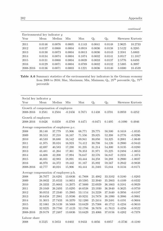
202 Appendix
continued
Environmental key indicator y
Year Mean Median Min Max Q1 Q3 Skewness Kurtosis
2011 0.0146 0.0076 0.0005 0.1143 0.0041 0.0148 2.9625 10.2733
2012 0.0137 0.0068 0.0004 0.0918 0.0036 0.0138 2.5122 6.3285
2013 0.0130 0.0073 0.0004 0.0813 0.0036 0.0143 2.3581 5.6803
2014 0.0134 0.0074 0.0004 0.1074 0.0032 0.0141 3.0517 11.1017
2015 0.0131 0.0068 0.0004 0.0839 0.0033 0.0137 2.5776 6.6493
2016 0.0129 0.0071 0.0004 0.0789 0.0032 0.0132 2.5305 6.3997
2008-2016 0.0136 0.0071 0.0003 0.1221 0.0036 0.0140 3.0300 10.4539
Table A.6 Summary statistics of the environmental key indicators in the German economyfrom 2008 to 2016; Max, Maximum; Min, Minimum; Q1, 25
th percentile; Q3, 75th
percentile
Social key indicator y
Year Mean Median Min Max Q1 Q3 Skewness Kurtosis
Growth of compensation of employees
2008-2016 0.2581 0.2504 -0.2456 0.7671 0.1438 0.3701 0.0959 0.4252
Growth of employees
2008-2016 0.0426 0.0358 -0.3789 0.4471 -0.0471 0.1495 -0.1090 0.4946
Average compensation of employees p.c.
2008 39,140 37,779 15,906 68,771 29,775 50,500 0.1618 -1.0535
2009 39,553 37,218 16,167 71,556 29,825 52,398 0.2776 -0.9296
2010 40,533 38,680 16,542 69,941 30,050 53,325 0.2001 -1.0649
2011 41,975 39,824 16,923 74,412 30,798 54,126 0.2900 -0.9443
2012 42,697 40,583 17,230 81,235 31,214 54,300 0.3135 -0.8280
2013 43,481 41,264 17,361 76,353 31,971 55,225 0.2494 -1.0653
2014 44,608 42,200 17,994 76,647 32,576 56,847 0.2231 -1.1074
2015 46,031 42,983 18,891 83,444 34,258 58,288 0.2900 -1.0037
2016 46,970 44,372 19,442 81,167 35,892 59,567 0.2942 -0.9838
2008-2016 42,777 40,024 15,906 83,444 31,2401 55,044 0.3134 -0.8171
Average compensation of employees p.h.
2008 26.7077 24.8291 13.6836 41.7808 21.4982 33.3102 0.3180 -1.0283
2009 28.0832 25.8533 14.0651 49.5385 22.3940 35.2803 0.4109 -0.8332
2010 28.3333 25.8683 14.2075 47.5600 22.6929 36.1663 0.3181 -0.9929
2011 29.1049 26.2493 15.0295 48.6538 23.1930 36.3840 0.3625 -0.9759
2012 30.0553 27.2340 15.2905 53.1154 24.2228 37.3440 0.3956 -0.8187
2013 30.6458 27.2981 15.9596 49.9231 24.7878 38.1990 0.3986 -0.9901
2014 31.3015 27.7433 16.3370 52.1200 25.2414 39.2481 0.4191 -0.9604
2015 32.1061 28.5139 16.5668 53.6429 25.7308 40.1712 0.4234 -0.9610
2016 32.9225 29.7780 17.4123 52.1786 26.7676 41.7613 0.4256 -0.9522
2008-2016 29.9178 27.2487 13.6836 53.6429 23.4066 37.0156 0.4282 -0.7378
Labour share
2008 0.5525 0.5853 0.0402 0.9433 0.4056 0.6957 -0.3736 -0.4180
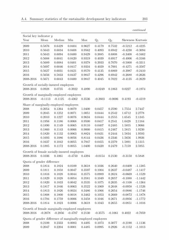
A.4. Summary statistics of the sustainable development key indicators 203
continued
Social key indicator y
Year Mean Median Min Max Q1 Q3 Skewness Kurtosis
2009 0.5876 0.6429 0.0404 0.9627 0.4179 0.7532 -0.5212 -0.4225
2010 0.5643 0.6034 0.0408 0.9562 0.4093 0.6942 -0.4230 -0.3094
2011 0.5643 0.6094 0.0400 0.9429 0.3885 0.6808 -0.3408 -0.3462
2012 0.5688 0.6041 0.0420 0.9319 0.4039 0.6917 -0.4006 -0.3166
2013 0.5689 0.6084 0.0401 0.9378 0.3933 0.7070 -0.5000 -0.3311
2014 0.5697 0.6046 0.0417 0.9334 0.4029 0.7001 -0.4271 -0.3507
2015 0.5627 0.6031 0.0421 0.9570 0.4135 0.6869 -0.3987 -0.2410
2016 0.5656 0.5833 0.0437 0.9847 0.4296 0.6942 -0.2688 -0.2626
2008-2016 0.5671 0.6043 0.0400 0.9847 0.4045 0.7022 -0.4135 -0.2629
Growth of socially-insured employees
2008-2016 0.0928 0.0735 -0.3922 0.4890 -0.0249 0.1863 0.0227 -0.1974
Growth of marginally-employed employees
2008-2016 -0.1113 -0.1125 -0.4362 0.3536 -0.2603 -0.0006 0.4193 -0.4219
Share of marginally-employed employees
2008 0.2054 0.1264 0.0079 1.0400 0.0457 0.2590 1.7554 2.7447
2009 0.2045 0.1252 0.0071 1.0051 0.0444 0.2542 1.6712 2.2778
2010 0.2010 0.1227 0.0076 0.9634 0.0444 0.2555 1.6545 2.1345
2011 0.1956 0.1186 0.0068 0.9500 0.0417 0.2541 1.6428 2.1164
2012 0.1890 0.1149 0.0065 0.9110 0.0407 0.2485 1.5855 1.9066
2013 0.1860 0.1143 0.0066 0.9000 0.0415 0.2467 1.5815 1.9230
2014 0.1820 0.1132 0.0063 0.8824 0.0431 0.2444 1.5834 1.9593
2015 0.1693 0.1086 0.0056 0.8144 0.0436 0.2346 1.5656 1.9926
2016 0.1637 0.1042 0.0055 0.7947 0.0455 0.2279 1.5891 2.1315
2008-2016 0.1885 0.1172 0.0055 1.0400 0.0420 0.2479 1.7159 2.5955
Growth of female socially-insured employees
2008-2016 0.1036 0.1061 -0.4750 0.4394 -0.0154 0.2130 -0.3150 0.5848
Quota of gender difference
2008 0.1814 0.1824 0.0109 0.3618 0.1036 0.2640 -0.0409 -1.1385
2009 0.1811 0.1858 0.0047 0.3597 0.1004 0.2637 -0.0487 -1.1417
2010 0.1816 0.1828 0.0044 0.3575 0.0989 0.2624 -0.0669 -1.1529
2011 0.1829 0.1828 0.0054 0.3581 0.1049 0.2657 -0.1088 -1.1442
2012 0.1820 0.1833 0.0042 0.3535 0.1075 0.2635 -0.1108 -1.1364
2013 0.1817 0.1846 0.0063 0.3522 0.1069 0.2648 -0.0958 -1.1526
2014 0.1813 0.1826 0.0024 0.3486 0.1066 0.2654 -0.0886 -1.1746
2015 0.1808 0.1800 0.0018 0.3462 0.1053 0.2669 -0.0872 -1.1878
2016 0.1794 0.1759 0.0006 0.3458 0.1046 0.2671 -0.0956 -1.1772
2008-2016 0.1814 0.1823 0.0006 0.3618 0.1043 0.2655 -0.0851 -1.1016
Growth of female marginally-employed employees
2008-2016 -0.2078 -0.2056 -0.4707 0.2130 -0.3575 -0.1061 0.4022 -0.7059
Quota of gender difference of marginally-employed employees
2008 0.2109 0.2333 0.0083 0.4495 0.1073 0.3077 -0.2190 -1.1136
2009 0.2047 0.2204 0.0001 0.4485 0.0995 0.2926 -0.1152 -1.1013
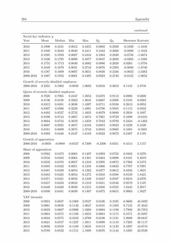
204 Appendix
continued
Social key indicator y
Year Mean Median Min Max Q1 Q3 Skewness Kurtosis
2010 0.1996 0.2101 0.0012 0.4355 0.0902 0.2939 -0.1039 -1.1649
2011 0.1940 0.2043 0.0048 0.4411 0.1042 0.2866 -0.0890 -1.1043
2012 0.1895 0.1959 0.0007 0.4316 0.1004 0.2830 -0.0738 -1.0674
2013 0.1826 0.1795 0.0090 0.4077 0.0947 0.2689 -0.0305 -1.1088
2014 0.1755 0.1713 0.0040 0.4062 0.0986 0.2626 0.0265 -1.0756
2015 0.1649 0.1679 0.0031 0.3742 0.0876 0.2393 -0.0093 -1.0740
2016 0.1587 0.1609 0.0007 0.3651 0.0820 0.2346 -0.0023 -1.0263
2008-2016 0.1867 0.1952 0.0001 0.4495 0.0923 0.2740 -0.0125 -1.0052
Growth of severely-disabled employees
2008-2016 0.2331 0.1962 -0.8048 1.0693 0.0816 0.3610 0.1145 2.3748
Quota of severely-disabled employees
2008 0.7820 0.7965 0.2447 1.3053 0.6378 0.9112 0.0906 0.0308
2009 0.8136 0.8198 0.3263 1.3645 0.6667 0.9398 0.2105 0.0382
2010 0.8312 0.8381 0.3030 1.4397 0.6711 0.9538 0.2613 0.0953
2011 0.8307 0.8386 0.3229 1.4091 0.6790 0.9505 0.1115 0.0332
2012 0.8492 0.8537 0.3722 1.4935 0.6979 0.9680 0.2958 0.1697
2013 0.8590 0.8744 0.3867 1.4674 0.7061 0.9720 0.1699 -0.0416
2014 0.8604 0.8734 0.3859 1.4350 0.7042 0.9793 0.2424 -0.1462
2015 0.8697 0.8925 0.3857 1.6183 0.6924 0.9833 0.4229 0.1620
2016 0.8581 0.8809 0.3875 1.3743 0.6916 0.9869 0.1085 -0.5001
2008-2016 0.8393 0.8440 0.2447 1.6183 0.6822 0.9673 0.2407 0.1195
Growth of apprentices
2008-2016 -0.0950 -0.0889 -0.6537 0.7309 -0.2206 0.0351 0.4514 2.1157
Share of apprentices
2008 0.0562 0.0473 0.0065 0.1407 0.0393 0.0722 0.9402 0.5276
2009 0.0558 0.0482 0.0064 0.1381 0.0404 0.0696 0.8101 0.4919
2010 0.0532 0.0476 0.0057 0.1310 0.0395 0.0672 0.7368 0.5472
2011 0.0495 0.0432 0.0051 0.1258 0.0366 0.0633 0.7707 0.7991
2012 0.0491 0.0439 0.0054 0.1262 0.0377 0.0612 0.8356 1.3821
2013 0.0482 0.0435 0.0054 0.1272 0.0358 0.0598 0.9129 1.8421
2014 0.0471 0.0431 0.0050 0.1249 0.0347 0.0587 0.9218 2.0376
2015 0.0457 0.0433 0.0042 0.1219 0.0341 0.0546 0.9579 2.1107
2016 0.0449 0.0430 0.0039 0.1215 0.0338 0.0525 1.0445 2.3917
2008-2016 0.0500 0.0441 0.0039 0.1407 0.0375 0.0615 0.9963 1.5627
VAT intensity
2008 0.0924 0.0637 -0.1069 2.0527 0.0106 0.1035 6.8608 48.8492
2009 0.0961 0.0656 -0.1149 1.9647 0.0101 0.1203 6.7125 47.4342
2010 0.0823 0.0607 -0.0996 1.3269 0.0094 0.1196 5.7892 38.7353
2011 0.0904 0.0575 -0.1166 1.9224 0.0084 0.1174 6.5571 45.9287
2012 0.0834 0.0575 -0.3102 1.6769 0.0100 0.1131 5.8098 39.6847
2013 0.0821 0.0557 -0.1237 1.3911 0.0099 0.1110 5.7205 38.1117
2014 0.0898 0.0550 -0.1169 1.8645 0.0112 0.1133 6.4297 44.6718
2015 0.0788 0.0532 -0.1151 1.1808 0.0076 0.1144 5.1695 32.9538
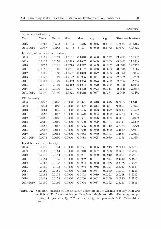
A.4. Summary statistics of the sustainable development key indicators 205
continued
Social key indicator y
Year Mean Median Min Max Q1 Q3 Skewness Kurtosis
2016 0.0767 0.0513 -0.1108 1.0816 0.0086 0.1107 4.7974 29.6315
2008-2016 0.0858 0.0583 -0.3102 2.0527 0.0090 0.1162 6.7882 52.5273
Intensity of net taxes on products
2008 0.0153 0.0173 -0.3144 0.1610 0.0086 0.0347 -3.2862 15.2532
2009 0.0132 0.0158 -0.2929 0.1037 0.0080 0.0333 -3.8463 17.0385
2010 0.0097 0.0121 -0.3278 0.1217 0.0033 0.0287 -3.3638 14.9952
2011 0.0129 0.0130 -0.2791 0.1107 0.0056 0.0338 -3.0039 12.5115
2012 0.0159 0.0130 -0.2567 0.1043 0.0072 0.0358 -3.0055 13.3004
2013 0.0146 0.0129 -0.2122 0.0995 0.0061 0.0333 -2.6728 10.7209
2014 0.0156 0.0139 -0.2460 0.1263 0.0073 0.0329 -2.8453 12.8765
2015 0.0146 0.0139 -0.2412 0.1284 0.0072 0.0309 -2.6529 11.9293
2016 0.0145 0.0139 -0.2507 0.1302 0.0073 0.0311 -2.6640 12.7958
2008-2016 0.0140 0.0140 -0.3278 0.1610 0.0067 0.0331 -3.2438 15.2486
CIT intensity
2008 0.0043 0.0028 0.0000 0.0321 0.0016 0.0045 3.2890 11.5411
2009 0.0044 0.0030 0.0000 0.0327 0.0014 0.0051 3.3081 12.2824
2010 0.0064 0.0045 0.0000 0.0485 0.0023 0.0072 3.3515 12.7592
2011 0.0083 0.0057 0.0000 0.0578 0.0034 0.0092 3.1430 11.1754
2012 0.0086 0.0058 0.0000 0.0601 0.0026 0.0088 3.0365 10.2052
2013 0.0090 0.0066 0.0000 0.0630 0.0029 0.0101 3.2415 12.0399
2014 0.0087 0.0067 0.0000 0.0605 0.0029 0.0112 3.2465 12.4870
2015 0.0086 0.0062 0.0000 0.0649 0.0030 0.0090 3.4070 13.8647
2016 0.0087 0.0063 0.0000 0.0683 0.0030 0.0101 3.4635 14.5648
2008-2016 0.0074 0.0050 0.0000 0.0683 0.0025 0.0080 3.5376 15.1636
Local business tax intensity
2008 0.0172 0.0144 0.0000 0.0771 0.0085 0.0218 2.2310 6.8476
2009 0.0187 0.0164 0.0000 0.0910 0.0087 0.0263 2.1599 7.5294
2010 0.0170 0.0154 0.0000 0.0901 0.0082 0.0212 2.5591 9.5505
2011 0.0194 0.0175 0.0000 0.0962 0.0101 0.0247 2.4412 8.3855
2012 0.0198 0.0178 0.0000 0.0994 0.0090 0.0238 2.3458 7.5485
2013 0.0189 0.0173 0.0000 0.0934 0.0086 0.0227 2.5317 8.9029
2014 0.0189 0.0181 0.0000 0.0812 0.0087 0.0230 1.9393 5.4216
2015 0.0188 0.0178 0.0000 0.0803 0.0089 0.0221 2.0268 5.5312
2016 0.0188 0.0178 0.0000 0.0800 0.0091 0.0229 2.0530 5.3517
2008-2016 0.0186 0.0166 0.0000 0.0994 0.0087 0.0232 2.3247 7.6911
Table A.7 Summary statistics of the social key indicators in the German economy from 2008to 2016; CIT, Corporate Income Tax; Max, Maximum; Min, Minimum; p.c., percapita; p.h., per hour; Q1, 25
th percentile; Q3, 75th percentile; VAT, Value Added
Tax

206 Appendix
Economic key indicator y
Year Mean Median Min Max Q1 Q3 Skewness Kurtosis
Gross capital productivity
2008 0.8185 0.3238 0.0409 10.2611 0.1969 0.6527 4.5418 20.7242
2009 0.7150 0.2989 0.0391 8.1873 0.2022 0.6935 4.4190 19.8595
2010 0.7520 0.3259 0.0382 9.6093 0.1944 0.6302 4.5956 21.6902
2011 0.7540 0.3525 0.0385 9.8559 0.1909 0.6358 4.6739 22.6935
2012 0.7339 0.3567 0.0364 9.3491 0.1868 0.5866 4.6423 22.7405
2013 0.7412 0.3563 0.0362 9.7401 0.1915 0.5997 4.7230 23.8312
2014 0.7434 0.3723 0.0353 9.6715 0.1882 0.6102 4.7076 23.5246
2015 0.7459 0.3841 0.0352 9.5349 0.1960 0.6303 4.7149 23.7958
2016 0.7303 0.3874 0.0346 8.4730 0.2017 0.6466 4.4713 21.3951
2008-2016 0.7482 0.3577 0.0346 10.2611 0.1905 0.6488 4.7617 23.5961
Net capital productivity
2008 1.5360 0.7208 0.0651 19.5957 0.3692 1.2737 4.5891 21.2061
2009 1.3412 0.6696 0.0628 15.3358 0.3619 1.2914 4.4387 20.0417
2010 1.4012 0.7110 0.0618 16.7112 0.3763 1.2103 4.5124 20.7685
2011 1.3871 0.7394 0.0627 16.1049 0.3761 1.2932 4.4752 20.6132
2012 1.3549 0.7558 0.0597 15.4591 0.3771 1.1981 4.4391 20.6293
2013 1.3698 0.7353 0.0598 16.2299 0.3843 1.2024 4.5107 21.6411
2014 1.3806 0.7431 0.0586 16.3239 0.3807 1.2374 4.5241 21.6233
2015 1.3989 0.7669 0.0589 16.5517 0.3851 1.2372 4.5664 22.1342
2016 1.3795 0.7856 0.0582 15.1008 0.3963 1.2867 4.3948 20.4261
2008-2016 1.3944 0.7378 0.0582 19.5957 0.3754 1.2488 4.6758 22.7766
Degree of modernity
2008 0.5265 0.5287 0.3522 0.6462 0.4858 0.5809 -0.3294 -0.4590
2009 0.5236 0.5295 0.3549 0.6359 0.4846 0.5712 -0.3188 -0.4255
2010 0.5225 0.5302 0.3596 0.6490 0.4818 0.5684 -0.2637 -0.3971
2011 0.5222 0.5312 0.3680 0.6368 0.4818 0.5635 -0.2775 -0.4788
2012 0.5204 0.5296 0.3769 0.6197 0.4833 0.5636 -0.3439 -0.4840
2013 0.5183 0.5241 0.3854 0.6200 0.4830 0.5632 -0.3664 -0.5066
2014 0.5172 0.5193 0.3980 0.6161 0.4827 0.5607 -0.3690 -0.5220
2015 0.5163 0.5231 0.3999 0.6143 0.4854 0.5566 -0.3972 -0.4005
2016 0.5160 0.5236 0.3980 0.6135 0.4879 0.5517 -0.3761 -0.2630
2008-2016 0.5203 0.5246 0.3522 0.6490 0.4839 0.5640 -0.3048 -0.2896
Consumed capital productivity
2008 11.5439 6.6066 1.1992 115.1420 3.8919 12.8816 4.4002 22.8315
2009 10.3365 5.9400 1.1023 93.2455 3.6583 13.4676 4.0937 20.5200
2010 10.8589 6.1751 1.0956 116.7000 3.8318 11.9480 4.9387 28.9186
2011 10.9139 6.5692 1.0897 119.8667 3.6428 12.0642 5.1386 31.0443
2012 10.5720 6.4374 1.0348 107.2395 3.6173 11.6762 4.8873 28.8094
2013 10.6097 6.5304 1.0376 108.7338 3.7812 11.4374 4.9492 29.4587
2014 10.6087 6.6479 1.1023 104.4061 3.6628 11.4133 4.7826 27.8628
2015 10.6090 7.0677 1.1415 98.7944 3.7356 11.7030 4.6440 26.6881
2016 10.4520 7.3297 1.1113 87.5120 3.9282 11.9263 4.2165 22.8075
2008-2016 10.7227 6.5277 1.0348 119.8667 3.6716 12.0207 4.8856 28.9152
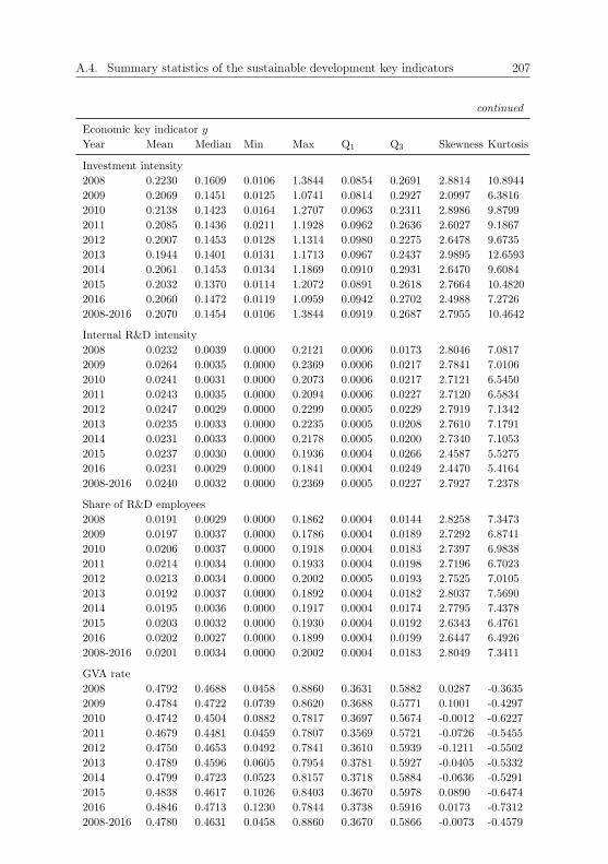
A.4. Summary statistics of the sustainable development key indicators 207
continued
Economic key indicator y
Year Mean Median Min Max Q1 Q3 Skewness Kurtosis
Investment intensity
2008 0.2230 0.1609 0.0106 1.3844 0.0854 0.2691 2.8814 10.8944
2009 0.2069 0.1451 0.0125 1.0741 0.0814 0.2927 2.0997 6.3816
2010 0.2138 0.1423 0.0164 1.2707 0.0963 0.2311 2.8986 9.8799
2011 0.2085 0.1436 0.0211 1.1928 0.0962 0.2636 2.6027 9.1867
2012 0.2007 0.1453 0.0128 1.1314 0.0980 0.2275 2.6478 9.6735
2013 0.1944 0.1401 0.0131 1.1713 0.0967 0.2437 2.9895 12.6593
2014 0.2061 0.1453 0.0134 1.1869 0.0910 0.2931 2.6470 9.6084
2015 0.2032 0.1370 0.0114 1.2072 0.0891 0.2618 2.7664 10.4820
2016 0.2060 0.1472 0.0119 1.0959 0.0942 0.2702 2.4988 7.2726
2008-2016 0.2070 0.1454 0.0106 1.3844 0.0919 0.2687 2.7955 10.4642
Internal R&D intensity
2008 0.0232 0.0039 0.0000 0.2121 0.0006 0.0173 2.8046 7.0817
2009 0.0264 0.0035 0.0000 0.2369 0.0006 0.0217 2.7841 7.0106
2010 0.0241 0.0031 0.0000 0.2073 0.0006 0.0217 2.7121 6.5450
2011 0.0243 0.0035 0.0000 0.2094 0.0006 0.0227 2.7120 6.5834
2012 0.0247 0.0029 0.0000 0.2299 0.0005 0.0229 2.7919 7.1342
2013 0.0235 0.0033 0.0000 0.2235 0.0005 0.0208 2.7610 7.1791
2014 0.0231 0.0033 0.0000 0.2178 0.0005 0.0200 2.7340 7.1053
2015 0.0237 0.0030 0.0000 0.1936 0.0004 0.0266 2.4587 5.5275
2016 0.0231 0.0029 0.0000 0.1841 0.0004 0.0249 2.4470 5.4164
2008-2016 0.0240 0.0032 0.0000 0.2369 0.0005 0.0227 2.7927 7.2378
Share of R&D employees
2008 0.0191 0.0029 0.0000 0.1862 0.0004 0.0144 2.8258 7.3473
2009 0.0197 0.0037 0.0000 0.1786 0.0004 0.0189 2.7292 6.8741
2010 0.0206 0.0037 0.0000 0.1918 0.0004 0.0183 2.7397 6.9838
2011 0.0214 0.0034 0.0000 0.1933 0.0004 0.0198 2.7196 6.7023
2012 0.0213 0.0034 0.0000 0.2002 0.0005 0.0193 2.7525 7.0105
2013 0.0192 0.0037 0.0000 0.1892 0.0004 0.0182 2.8037 7.5690
2014 0.0195 0.0036 0.0000 0.1917 0.0004 0.0174 2.7795 7.4378
2015 0.0203 0.0032 0.0000 0.1930 0.0004 0.0192 2.6343 6.4761
2016 0.0202 0.0027 0.0000 0.1899 0.0004 0.0199 2.6447 6.4926
2008-2016 0.0201 0.0034 0.0000 0.2002 0.0004 0.0183 2.8049 7.3411
GVA rate
2008 0.4792 0.4688 0.0458 0.8860 0.3631 0.5882 0.0287 -0.3635
2009 0.4784 0.4722 0.0739 0.8620 0.3688 0.5771 0.1001 -0.4297
2010 0.4742 0.4504 0.0882 0.7817 0.3697 0.5674 -0.0012 -0.6227
2011 0.4679 0.4481 0.0459 0.7807 0.3569 0.5721 -0.0726 -0.5455
2012 0.4750 0.4653 0.0492 0.7841 0.3610 0.5939 -0.1211 -0.5502
2013 0.4789 0.4596 0.0605 0.7954 0.3781 0.5927 -0.0405 -0.5332
2014 0.4799 0.4723 0.0523 0.8157 0.3718 0.5884 -0.0636 -0.5291
2015 0.4838 0.4617 0.1026 0.8403 0.3670 0.5978 0.0890 -0.6474
2016 0.4846 0.4713 0.1230 0.7844 0.3738 0.5916 0.0173 -0.7312
2008-2016 0.4780 0.4631 0.0458 0.8860 0.3670 0.5866 -0.0073 -0.4579

208 Appendix
continued
Economic key indicator y
Year Mean Median Min Max Q1 Q3 Skewness Kurtosis
Growth of working population
2008-2016 0.0254 0.0205 -0.3763 0.3393 -0.0512 0.1129 -0.2320 0.3135
Labour productivity p.c.
2008 83,714 58,713 20,113 568,205 43,433 89,709 3.5559 15.4814
2009 80,662 54,075 18,989 573,754 40,740 82,131 3.6039 15.9809
2010 86,576 57,059 19,804 577,276 43,595 96,779 3.2723 12.9202
2011 86,779 59,897 20,773 608,305 45,196 97,475 3.7824 18.0996
2012 87,675 60,133 21,499 596,640 45,705 96,739 3.5958 16.5577
2013 89,753 61,721 20,852 630,222 46,046 96,315 3.7517 17.6535
2014 90,118 63,410 21,846 633,637 48,607 100,820 4.0163 20.4509
2015 96,000 66,191 23,383 644,676 51,370 109,415 3.5961 16.3852
2016 97,914 68,836 23,837 660,073 51,159 109,285 3.6413 16.5231
2008-2016 88,799 59,897 18,989 66,0073 45,991 96,803 3.7307 17.3894
Labour productivity p.h.
2008 51.6057 36.3282 14.3602 463.3060 31.0183 51.7074 5.6110 35.6733
2009 51.3303 36.2651 13.8568 470.3569 30.7558 56.2915 5.4967 34.3859
2010 54.8477 37.4930 14.5352 469.7346 30.7674 58.5954 4.8999 27.8048
2011 54.8121 37.5007 15.5386 504.7401 30.9396 56.3481 5.7151 36.9783
2012 56.3741 38.6033 16.5086 499.3387 31.8539 60.6704 5.4545 34.2123
2013 58.1160 40.6606 16.4775 538.8513 33.8150 61.3120 5.6866 36.3289
2014 58.7549 40.8332 17.5250 538.3009 35.7346 61.9106 5.8460 38.2331
2015 60.9196 42.2494 18.6414 545.7635 36.4462 62.8906 5.5248 34.6680
2016 63.1494 43.0463 19.2219 559.4446 36.4785 64.3460 5.4108 33.4357
2008-2016 56.6567 39.6446 13.8568 559.4446 33.9144 59.9764 5.6701 36.4428
Net import intensity
2008 0.1783 -0.0069 -1.8850 10.0502 -0.0428 -0.0034 5.1643 30.3137
2009 0.2097 -0.0052 -1.9642 11.9215 -0.0386 -0.0023 5.4430 33.8348
2010 0.1985 -0.0064 -2.0627 12.2980 -0.0425 -0.0006 6.0411 40.4506
2011 0.2881 -0.0055 -2.3804 15.3353 -0.0286 0.0031 5.7782 36.4375
2012 0.2413 -0.0027 -2.5228 15.4300 -0.0421 -0.0027 6.0742 40.4449
2013 0.2591 -0.0078 -2.1258 16.8597 -0.0643 0.0147 6.3208 42.7579
2014 0.2344 -0.0121 -2.4746 15.6015 -0.0703 -0.0092 5.9848 39.1775
2015 0.1652 -0.0121 -2.6442 12.4731 -0.0850 -0.0121 5.7149 37.7941
2016 0.1267 -0.0131 -3.3450 11.2043 -0.0363 -0.0131 5.2493 34.6466
2008-2016 0.2112 -0.0121 -3.3450 16.8597 -0.0488 -0.0027 6.2108 43.7853
Share of imported input
2008 0.1834 0.1330 0.0218 0.7231 0.0854 0.2495 1.4618 2.1279
2009 0.1773 0.1288 0.0210 0.7415 0.0795 0.2403 1.8248 3.9068
2010 0.1956 0.1476 0.0203 0.7140 0.0848 0.2869 1.4522 2.3560
2011 0.1974 0.1432 0.0186 0.7641 0.0879 0.2890 1.4350 2.5109
2012 0.2042 0.1524 0.0188 0.7725 0.0946 0.2827 1.4617 2.5433
2013 0.2043 0.1442 0.0358 0.7610 0.0959 0.2921 1.5133 2.7375
2014 0.2007 0.1453 0.0328 0.7356 0.0937 0.2925 1.4219 2.2985
2015 0.2052 0.1424 0.0326 0.7119 0.0962 0.3071 1.2011 1.3309

A.5. Outlier thresholds of the sustainable development key indicators 209
continued
Economic key indicator y
Year Mean Median Min Max Q1 Q3 Skewness Kurtosis
2016 0.2074 0.1444 0.0295 0.7695 0.0955 0.3053 1.6098 2.9522
2008-2016 0.1973 0.1424 0.0186 0.7725 0.0905 0.2904 1.5176 2.6939
Table A.8 Summary statistics of the economic key indicators in the German economy from2008 to 2016; GVA, Gross Value Added; Max, Maximum; Min, Minimum; p.c.,per capita; p.h., per hour; Q1, 25
th percentile; Q3, 75th percentile; R&D, Research
and Development
A.5 Outlier thresholds of the sustainable develop-
ment key indicators
Environmental key indicator y Lower thresh-old θmin
Upper thresh-old θmax
Growth of air emissions -0.5912 0.5740
Air emissions intensity -305.1278† 619.6294
Growth of primary energy consumption -0.4546 0.4012
Energy intensity -4.7559† 10.5097
Growth of water use -0.4870 0.4754
Water intensity -3.3779† 6.1136
Growth of waste water -0.4823 0.4286
Waste water intensity -1.5134† 2.8812
Growth of hazardous waste -0.9767 0.8390
Hazardous waste intensity -8.6396† 15.9854
Environmental tax intensity -0.0121† 0.0297
Table A.9 Environmental key indicators’ upper and lower outlier thresholds; †, theoreticalthreshold (domain ≥ 0)
Social key indicator y Lower thresh-old θmin
Upper thresh-old θmax
Growth of compensation of employees -0.1957 0.7095
Growth of employees -0.3420 0.4444
Average compensation of employees p.c. -4,463.27† 90,748.08
Average compensation of employees p.h. 2.9932 57.4291
Labour share -0.0420† 1.1488

210 Appendix
continued
Social key indicator y Lower thresh-old θmin
Upper thresh-old θmax
Growth of socially-insured employees -0.3416 0.5031
Growth of marginally-employed employ-ees
-0.6498 0.3889
Share of marginally-employed employees -0.2668† 0.5567
Growth of female socially-insured em-ployees
-0.3579 0.5555
Quota of gender difference -0.1376 0.5073
Growth of female marginally-employedemployees
-0.7346 0.2710
Quota of gender difference of marginally-employed employees
-0.1802 0.5465
Growth of severely-disabled employees -0.3376 0.7802
Quota of severely-disabled employees 0.2546 1.3949
Growth of apprentices -0.6041 0.4186
Share of apprentices 0.0014 0.0976
VAT intensity -0.1519 0.2771
Intensity of net taxes on products -0.0328 0.0726
CIT intensity -0.0058† 0.0163
Local business tax intensity -0.0130† 0.0449
Table A.10 Social key indicators’ upper and lower outlier thresholds; †, theoretical threshold(domain ≥ 0); CIT, Corporate Income Tax; p.c., per capita; p.h., per hour; VAT,Value Added Tax
Economic key indicator y Lower thresh-old θmin
Upper thresh-old θmax
Gross capital productivity -0.4969† 1.3362
Net capital productivity -0.9346† 2.5589
Degree of modernity 0.3638 0.6841
Consumed capital productivity -8.8522† 24.5445
Investment intensity -0.1733† 0.5340
Internal R&D intensity -0.0329† 0.0561
Share of R&D employees -0.0264† 0.0451
GVA rate 0.0376 0.9160
Growth of working population -0.2974 0.3591

A.6. Normality tests of z-score scaled sustainable development key indicators 211
continued
Economic key indicator y Lower thresh-old θmin
Upper thresh-old θmax
Labour productivity p.c. -30,228.50† 17,3022.17
Labour productivity p.h. -5.1786† 99.0694
Net import intensity -0.1180 0.0665
Share of imported input -0.2093 0.5902
Table A.11 Economic key indicators’ upper and lower outlier thresholds; †, theoreticalthreshold (domain ≥ 0); GVA, Gross Value Added; p.c., per capita; p.h., perhour; R&D, Research and Development
A.6 Normality tests of z-score scaled sustainable
development key indicators
Z-score scaled environmental key indic-ator yz
SW stat-istic
SWp-values
KS stat-istic
KSp-values
Reduction of air emissions 0.9666 0.0891 0.1242 0.2944
Air emissions efficiency 0.6910 0.0000 0.2928 0.0001
Reduction of primary energy consump-tion
0.9694 0.1235 0.0900 0.6973
Energy efficiency 0.7343 0.0000 0.2504 0.0009
Reduction of water use 0.9876 0.7890 0.0485 0.9986
Water efficiency 0.6909 0.0000 0.2875 0.0002
Reduction of waste water 0.9828 0.5331 0.0614 0.9734
Waste water efficiency 0.7558 0.0000 0.2234 0.0077
Reduction of hazardous waste 0.9618 0.0512 0.0886 0.7148
Hazardous waste efficiency 0.7350 0.0000 0.2759 0.0004
Environmental tax intensity 0.8254 0.0000 0.1747 0.0471
Table A.12 Z-score scaled environmental key indicators’ average test statistics and p-valuesof the Shapiro-Wilk (SW) and the Kolmogorov-Smirnov (KS) tests from 2008to 2016
Z-score scaled social key indicator yz SW stat-istic
SWp-values
KS stat-istic
KSp-values
Growth of compensation of employees 0.9815 0.4721 0.0788 0.8357
Growth of employees 0.9887 0.8408 0.0808 0.8131
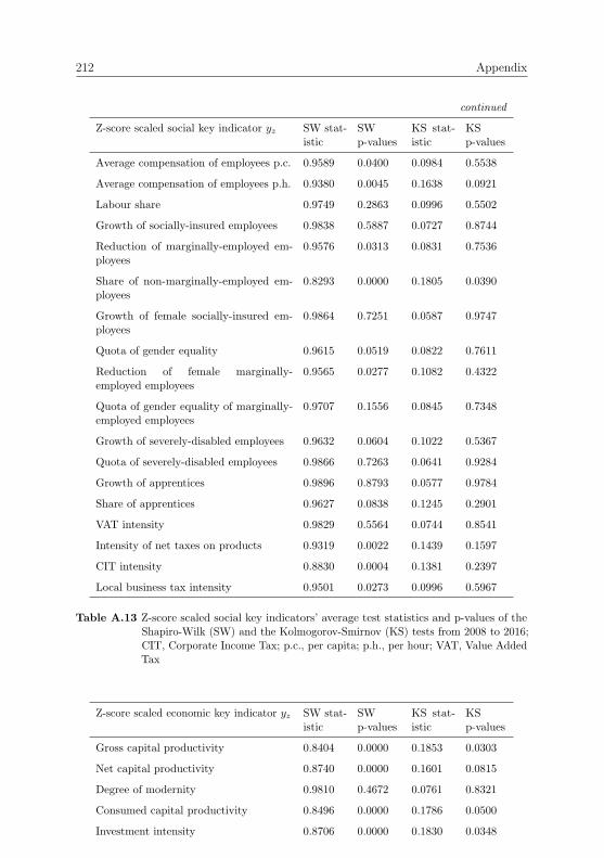
212 Appendix
continued
Z-score scaled social key indicator yz SW stat-istic
SWp-values
KS stat-istic
KSp-values
Average compensation of employees p.c. 0.9589 0.0400 0.0984 0.5538
Average compensation of employees p.h. 0.9380 0.0045 0.1638 0.0921
Labour share 0.9749 0.2863 0.0996 0.5502
Growth of socially-insured employees 0.9838 0.5887 0.0727 0.8744
Reduction of marginally-employed em-ployees
0.9576 0.0313 0.0831 0.7536
Share of non-marginally-employed em-ployees
0.8293 0.0000 0.1805 0.0390
Growth of female socially-insured em-ployees
0.9864 0.7251 0.0587 0.9747
Quota of gender equality 0.9615 0.0519 0.0822 0.7611
Reduction of female marginally-employed employees
0.9565 0.0277 0.1082 0.4322
Quota of gender equality of marginally-employed employees
0.9707 0.1556 0.0845 0.7348
Growth of severely-disabled employees 0.9632 0.0604 0.1022 0.5367
Quota of severely-disabled employees 0.9866 0.7263 0.0641 0.9284
Growth of apprentices 0.9896 0.8793 0.0577 0.9784
Share of apprentices 0.9627 0.0838 0.1245 0.2901
VAT intensity 0.9829 0.5564 0.0744 0.8541
Intensity of net taxes on products 0.9319 0.0022 0.1439 0.1597
CIT intensity 0.8830 0.0004 0.1381 0.2397
Local business tax intensity 0.9501 0.0273 0.0996 0.5967
Table A.13 Z-score scaled social key indicators’ average test statistics and p-values of theShapiro-Wilk (SW) and the Kolmogorov-Smirnov (KS) tests from 2008 to 2016;CIT, Corporate Income Tax; p.c., per capita; p.h., per hour; VAT, Value AddedTax
Z-score scaled economic key indicator yz SW stat-istic
SWp-values
KS stat-istic
KSp-values
Gross capital productivity 0.8404 0.0000 0.1853 0.0303
Net capital productivity 0.8740 0.0000 0.1601 0.0815
Degree of modernity 0.9810 0.4672 0.0761 0.8321
Consumed capital productivity 0.8496 0.0000 0.1786 0.0500
Investment intensity 0.8706 0.0000 0.1830 0.0348
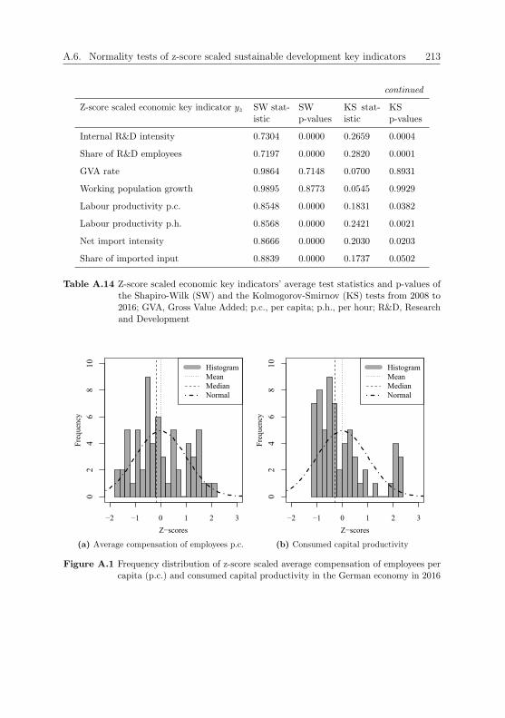
A.6. Normality tests of z-score scaled sustainable development key indicators 213
continued
Z-score scaled economic key indicator yz SW stat-istic
SWp-values
KS stat-istic
KSp-values
Internal R&D intensity 0.7304 0.0000 0.2659 0.0004
Share of R&D employees 0.7197 0.0000 0.2820 0.0001
GVA rate 0.9864 0.7148 0.0700 0.8931
Working population growth 0.9895 0.8773 0.0545 0.9929
Labour productivity p.c. 0.8548 0.0000 0.1831 0.0382
Labour productivity p.h. 0.8568 0.0000 0.2421 0.0021
Net import intensity 0.8666 0.0000 0.2030 0.0203
Share of imported input 0.8839 0.0000 0.1737 0.0502
Table A.14 Z-score scaled economic key indicators’ average test statistics and p-values ofthe Shapiro-Wilk (SW) and the Kolmogorov-Smirnov (KS) tests from 2008 to2016; GVA, Gross Value Added; p.c., per capita; p.h., per hour; R&D, Researchand Development
Z−scores
Freq
uenc
y0
24
68
10
−2 −1 0 1 2 3
HistogramMeanMedianNormal
(a) Average compensation of employees p.c.
Z−scores
Freq
uenc
y0
24
68
10
−2 −1 0 1 2 3
HistogramMeanMedianNormal
(b) Consumed capital productivity
Figure A.1 Frequency distribution of z-score scaled average compensation of employees percapita (p.c.) and consumed capital productivity in the German economy in 2016
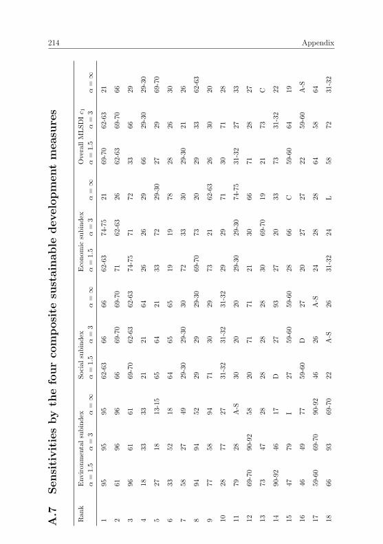
214 Appendix
A.7
Sensitivitiesbyth
efourco
mposite
sustainable
developmentmeasu
res
Rank
Environmentalsubindex
Socialsubindex
Economic
subindex
OverallMLSDIc 1
α=
1.5
α=
3α=
∞α=
1.5
α=
3α=
∞α=
1.5
α=
3α=
∞α=
1.5
α=
3α=
∞1
9595
9562-63
66
6662
-63
74-75
2169
-70
62-63
21
261
9696
66
69-70
69-70
7162
-63
2662
-63
69-70
66
396
6161
69-70
62-63
62-63
74-75
7172
3366
29
418
3333
2121
6426
2629
6629-30
29-30
527
1813
-15
65
64
2133
7229
-30
2729
69-70
633
5218
6465
6519
1978
2826
30
758
2749
29-30
29-30
3072
3330
29-30
2126
894
9452
29
2929
-30
69-70
7320
2933
62-63
977
5894
71
3029
7321
62-63
2630
20
1028
7727
31-32
31-32
31-32
2929
7130
7128
1179
28A-S
3020
2029
-30
29-30
74-75
31-32
2733
1269
-70
90-92
5820
71
7121
3066
7128
27
1373
4728
28
2828
3069
-70
1921
73C
1490
-92
4617
D27
9327
2033
7331
-32
22
15
47
79
I27
59-60
59-60
28
66
C59-60
64
19
1646
4977
59-60
D27
2027
2722
59-60
A-S
17
59-60
69-70
90-92
46
26
A-S
24
28
28
64
58
64
1866
9369
-70
22
A-S
2631
-32
24L
5872
31-32
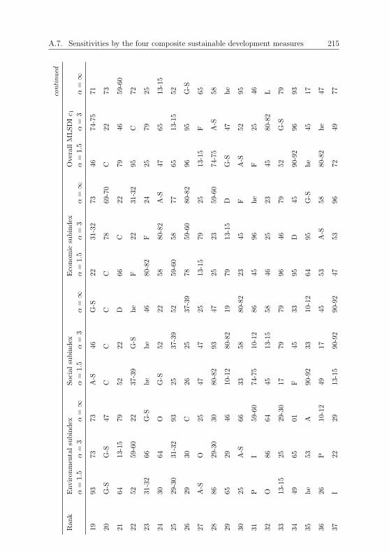
A.7. Sensitivities by the four composite sustainable development measures 215
continued
Rank
Environmentalsubindex
Socialsubindex
Economic
subindex
OverallMLSDIc 1
α=
1.5
α=
3α=
∞α=
1.5
α=
3α=
∞α=
1.5
α=
3α=
∞α=
1.5
α=
3α=
∞19
93
73
73
A-S
46
G-S
22
31-32
73
46
74-75
71
20
G-S
G-S
47
CC
CC
78
69-70
C22
73
2164
13-15
7952
22
D66
C22
7946
59-60
22
52
59-60
22
37-39
G-S
he
F22
31-32
95
C72
23
31-32
66
G-S
he
he
46
80-82
F24
25
79
25
24
30
64
OG-S
52
22
58
80-82
A-S
47
65
13-15
2529
-30
31-32
9325
37-39
5259
-60
5877
6513
-15
52
26
29
30
C26
25
37-39
78
59-60
80-82
96
95
G-S
27A-S
O25
47
4725
13-15
7925
13-15
F65
2886
29-30
3080-82
93
4725
2359
-60
74-75
A-S
58
29
65
29
46
10-12
80-82
19
79
13-15
DG-S
47
he
30
25
A-S
66
33
58
80-82
23
45
FA-S
52
95
31
PI
59-60
74-75
10-12
86
45
96
he
F25
46
32O
8664
45
13-15
5846
2523
4580
-82
L
33
13-15
25
29-30
17
79
79
96
46
79
52
G-S
79
3449
6501
F45
3395
D45
90-92
9693
35
he
53
A90-92
33
10-12
64
95
G-S
he
45
17
36
26
P10-12
49
17
45
53
A-S
58
80-82
he
47
37I
2229
13-15
90-92
90-92
4753
9672
4977

216 Appendix
continued
Rank
Environmentalsubindex
Socialsubindex
Economic
subindex
OverallMLSDIc 1
α=
1.5
α=
3α=
∞α=
1.5
α=
3α=
∞α=
1.5
α=
3α=
∞α=
1.5
α=
3α=
∞38
02
he
23
79
86
13-15
D64
53
49
90-92
90-92
3945
45P
86
74-75
74-75
A-S
4713
-15
8653
49
40L
2631
-32
19
F17
IL
3694
7724
41
22
F20
58
19
Fhe
he
46
77
86
96
4287
-88
0226
93
49
4916
I95
9393
23
43C
L21
23
36
7265
6517
5378
F
4453
87-88
8636
73
O49
G-S
37-39
1894
78
45
F62-63
53
24
23
73
G-S
49
II
L86
4662
-63
7824
87-88
72
3617
7752
6118
10-12
4778
C65
1624
2302
16B
PI
45
48
21
80-82
he
95
16
87-88
94
52
51
78
O80-82
49
80-82
21
19
72
87-88
51
52
02
64
O87-88
O
5071
7136
OO
2486
9490
-92
87-88
PI
5150
7202
51
5353
6136
86L
0236
5272
A45
53
5116
90-92
8647
0261
53
53A
74-75
F03
95
9510
-12
1887
-88
1616
37-39
5474
-75
03L
77L
L36
90-92
10-12
10-12
2094
5516
5087
-88
73
77
77B
B50
2403
87-88
56
03
16
16
P03
PP
17
P20
10-12
74-75

A.7. Sensitivities by the four composite sustainable development measures 217
continued
Rank
Environmentalsubindex
Socialsubindex
Economic
subindex
OverallMLSDIc 1
α=
1.5
α=
3α=
∞α=
1.5
α=
3α=
∞α=
1.5
α=
3α=
∞α=
1.5
α=
3α=
∞57
10-12
0151
96
II
LP
9403
AP
5801
10-12
62-63
IP
0303
37-39
65D
37-39
18
5937
-39
37-39
B94
96
9418
0303
A36
51
6051
3678
L94
9677
6149
37-39
DD
6136
5137
-39
50
18
B37
-39
10-12
0117
2316
62B
1703
78
B01
87-88
87-88
A36
2401
6317
2380
-82
18
50
A51
O93
2301
A
64D
B50
AA
50A
A18
5050
B
6524
2071
01
0118
O01
O51
1703
6623
D72
B02
0201
5102
1951
02
6720
24D
0278
7893
9316
0119
61
6819
1974
-75
61
61
6150
5061
BB
50
Table
A.15Rankingoftheeconomic
objectsin
StatisticalClassificationofEconomic
Activitiesin
theEuropeanCommunity(N
ACE)codes
bythe
fourcompositemeasuresan
dthethreeou
tlierdetection
methodsin
theGerman
econ
omyin
2016
;seeTab
leA.1
fordenotationof
section
codes;α,ou
tliercoeffi
cient;MLSDI,Multilevel
Sustainable
DevelopmentIndex
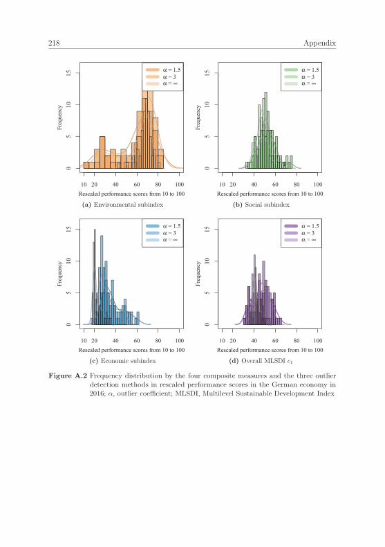
218 Appendix
Rescaled performance scores from 10 to 100
Freq
uenc
y0
510
15
10 20 40 60 80 100
α = 1.5α = 3α = ∞
(a) Environmental subindex
Rescaled performance scores from 10 to 100Fr
eque
ncy
05
1015
10 20 40 60 80 100
α = 1.5α = 3α = ∞
(b) Social subindex
Rescaled performance scores from 10 to 100
Freq
uenc
y0
510
15
10 20 40 60 80 100
α = 1.5α = 3α = ∞
(c) Economic subindex
Rescaled performance scores from 10 to 100
Freq
uenc
y0
510
15
10 20 40 60 80 100
α = 1.5α = 3α = ∞
(d) Overall MLSDI c1
Figure A.2 Frequency distribution by the four composite measures and the three outlierdetection methods in rescaled performance scores in the German economy in2016; α, outlier coefficient; MLSDI, Multilevel Sustainable Development Index
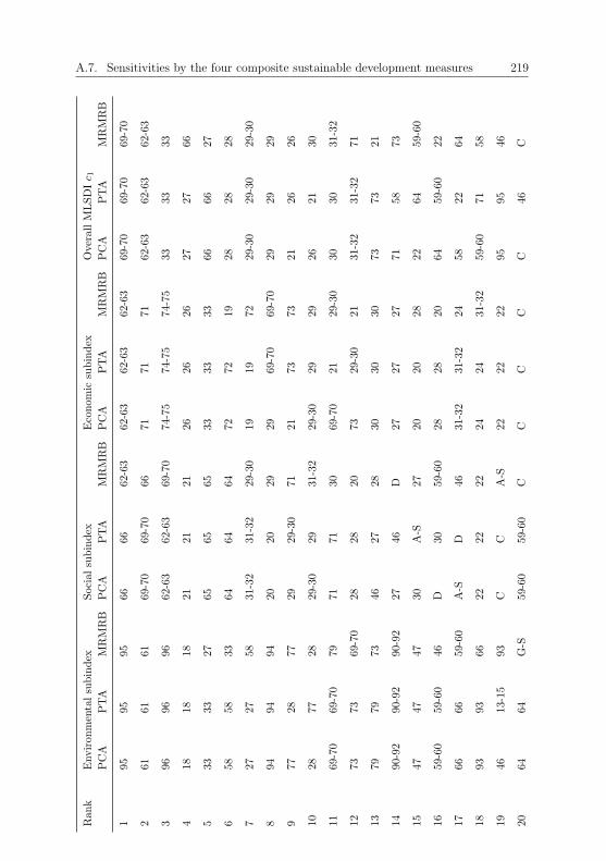
A.7. Sensitivities by the four composite sustainable development measures 219
Rank
Environmentalsubindex
Socialsubindex
Economic
subindex
OverallMLSDIc 1
PCA
PTA
MRMRB
PCA
PTA
MRMRB
PCA
PTA
MRMRB
PCA
PTA
MRMRB
195
95
95
66
66
62-63
62-63
62-63
62-63
69-70
69-70
69-70
261
6161
69-70
69-70
6671
7171
62-63
62-63
62-63
396
96
96
62-63
62-63
69-70
74-75
74-75
74-75
33
33
33
418
1818
2121
2126
2626
2727
66
533
3327
6565
6533
3333
6666
27
658
5833
6464
6472
7219
2828
28
727
27
58
31-32
31-32
29-30
19
19
72
29-30
29-30
29-30
894
9494
2020
2929
69-70
69-70
2929
29
977
2877
2929
-30
7121
7373
2126
26
1028
7728
29-30
2931
-32
29-30
2929
2621
30
1169
-70
69-70
79
71
7130
69-70
2129
-30
3030
31-32
1273
7369-70
2828
2073
29-30
2131
-32
31-32
71
1379
7973
4627
2830
3030
7373
21
1490
-92
90-92
90-92
27
46D
2727
2771
5873
1547
4747
30A-S
2720
2028
2264
59-60
1659
-60
59-60
46
D30
59-60
2828
2064
59-60
22
1766
6659-60
A-S
D46
31-32
31-32
2458
2264
1893
9366
2222
2224
2431
-32
59-60
7158
1946
13-15
93
CC
A-S
2222
2295
9546
20
64
64
G-S
59-60
59-60
CC
CC
C46
C

220 Appendix
continued
Rank
Environmentalsubindex
Socialsubindex
Economic
subindex
OverallMLSDIc 1
PCA
PTA
MRMRB
PCA
PTA
MRMRB
PCA
PTA
MRMRB
PCA
PTA
MRMRB
21G-S
4664
5252
5266
6666
46C
79
22
13-15
G-S
52
G-S
G-S
37-39
FF
F25
79
95
23
52
52
31-32
he
he
he
59-60
58
80-82
65
25
25
24
31-32
31-32
30
26
25
G-S
58
59-60
58
79
13-15
47
25
A-S
25
29-30
37-39
37-39
25
25
80-82
59-60
13-15
65
65
2625
A-S
2925
2626
80-82
7878
9696
96
27
29-30
30
A-S
10-12
10-12
47
78
25
13-15
47
47
13-15
28
P29-30
86
13-15
47
80-82
23
13-15
25
A-S
A-S
74-75
29
30
I65
80-82
17
10-12
13-15
45
79
G-S
G-S
G-S
3029
P25
47
4533
4579
2390
-92
45A-S
3186
29P
17
13-15
74-75
7923
4545
52F
32I
86O
45
80-82
4546
4646
5290
-92
45
33
OO
13-15
90-92
33
17
96
96
96
he
F52
34
65
65
49
33
74-75
F64
64
95
Fhe
90-92
35
49
49
he
74-75
90-92
90-92
95
95
64
74-75
61
he
3626
2626
58
F49
DD
5349
9480
-82
3722
22I
F36
13-15
5353
4794
7772
38
he
he
02
36
79
79
A-S
47
D80-82
49
49
3945
4545
49
5886
47A-S
A-S
6186
86
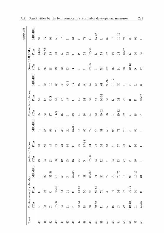
A.7. Sensitivities by the four composite sustainable development measures 221
continued
Rank
Environmentalsubindex
Socialsubindex
Economic
subindex
OverallMLSDIc 1
PCA
PTA
MRMRB
PCA
PTA
MRMRB
PCA
PTA
MRMRB
PCA
PTA
MRMRB
40L
LL
7993
1965
65I
7774
-75
94
41
02
02
22
93
86
58
he
he
he
86
80-82
77
42
CC
87-88
23
49
93
17
G-S
16
18
18
93
43
87-88
87-88
C86
19
23
G-S
16
65
93
93
53
4453
5353
19
2336
1617
4972
O18
45
21
21
F95
95
24
I49
G-S
53
72
I
46F
F62-63
16
O87
-88
49I
17O
I61
4762
-63
62-63
7824
16
1661
6102
IP
P
4878
5021
O87
-88
9536
9494
P53
78
4950
7880
-82
87-88
24
7294
3652
87-88
87-88
O
5080
-82
80-82
7153
72
O52
5286
LL
87-88
5171
7150
72
0351
90-92
90-92
6178
78L
52A
A72
51
5353
8686
90-92
0202
02
5316
16A
03
5103
LL
10-12
1616
16
5403
0374
-75
73
77
7710
-12
0236
2424
10-12
5572
7216
77
7373
0277
B20
10-12
24
5610
-12
10-12
03P
PP
77B
P10
-12
D20
5701
0110
-12
96
96
9618
PL
D20
03
5874
-75
B01
II
IP
10-12
0317
36D

222 Appendix
continued
Rank
Environmentalsubindex
Socialsubindex
Economic
subindex
OverallMLSDIc 1
PCA
PTA
MRMRB
PCA
PTA
MRMRB
PCA
PTA
MRMRB
PCA
PTA
MRMRB
59B
74-75
37-39
9494
94B
37-39
1836
17A
6036
3651
18
18L
5118
7750
5037
-39
6117
1736
LL
5037
-39
5137
-39
0303
17
62
DD
B50
50
78
03
03
87-88
23
37-39
36
6337
-39
2417
BB
18O
O51
37-39
2323
6424
37-39
D78
AA
87-88
87-88
AA
A50
6551
5124
A01
0193
93O
BB
51
6623
2323
01
78B
AA
0151
0119
6720
2020
02
0202
0101
9301
5101
6819
1919
61
6161
5050
5019
19B
Table
A.16Rankingoftheeconomic
objectsin
StatisticalClassificationofEconomic
Activitiesin
theEuropeanCommunity(N
ACE)codes
bythe
fourcompositemeasuresan
dthethreeweigh
tingmethodsin
theGerman
econ
omyin
2016
;seeTab
leA.1
fordenotationof
sectioncodes;
MLSDI,Multilevel
Sustainable
DevelopmentIndex;MRMRB,Maxim
um
Relevance
Minim
um
Red
undancy
Backward
algorithm;PCA,
PrincipalCompon
entAnalysis;
PTA,PartialTriadic
Analysis

Appendix 223
Rescaled performance scores from 10 to 100
Freq
uenc
y0
24
68
1012
14
10 20 40 60 80 100
PCAPTAMRMRB
(a) Environmental subindex
Rescaled performance scores from 10 to 100Fr
eque
ncy
02
46
810
1214
10 20 40 60 80 100
PCAPTAMRMRB
(b) Social subindex
Rescaled performance scores from 10 to 100
Freq
uenc
y0
24
68
1012
14
10 20 40 60 80 100
PCAPTAMRMRB
(c) Economic subindex
Rescaled performance scores from 10 to 100
Freq
uenc
y0
24
68
1012
14
10 20 40 60 80 100
PCAPTAMRMRB
(d) Overall MLSDI c1
Figure A.3 Frequency distribution of the four composite measures by the three weightingmethods in rescaled performance scores in the German economy in 2016; MLSDI,Multilevel Sustainable Development Index; MRMRB, Maximum Relevance Min-imum Redundancy Backward algorithm; PCA, Principal Component Analysis;PTA, Partial Triadic Analysis
References
A4S. (2018). A4S knowledge hub: Guides. Retrieved November 21, 2019, from https://www.accountingforsustainability.org/content/a4s/corporate/en/knowledge-hub.html?tab1=guides
Aggarwal, C. C. (2017). Outlier analysis (2nd Ed.). Cham: Springer.
Aggarwal, C. C. & Sathe, S. (2015). Theoretical foundations and algorithms for outlierensembles. SIGKDD Explorations, 17 (1), 24–47. doi:10.1145/2830544.2830549
Aggarwal, C. C. & Sathe, S. (2017). Outlier ensembles: An introduction. Cham: Springer.
Agyeman, J. (2005). Sustainable communities and the challenge of environmental justice.New York: New York University Press.
AIChE & IfS. (2019). American Institute of Chemical Engineers (AIChE) SustainabilityIndex. Retrieved November 21, 2019, from https://www.aiche.org/ifs/resources/sustainability-index
Ajmal, M. M., Khan, M., Hussain, M. & Helo, P. (2018). Conceptualizing and in-corporating social sustainability in the business world. International Journal ofSustainable Development & World Ecology, 25 (4), 327–339. doi:10.1080/13504509.2017.1408714
Alcacer, V. & Cruz-Machado, V. (2019). Scanning the industry 4.0: A literature reviewon technologies for manufacturing systems. Engineering Science and Technology,an International Journal, 22 (3), 899–919. doi:10.1016/j.jestch.2019.01.006
Allen, C., Metternicht, G. & Wiedmann, T. O. (2017). An iterative framework fornational scenario modelling for the Sustainable Development Goals (SDGs). Sus-tainable Development, 25 (5), 372–385. doi:10.1002/sd.1662
Allen, C., Metternicht, G. & Wiedmann, T. O. (2019). Prioritising SDG targets:Assessing baselines, gaps and interlinkages. Sustainability Science, 14 (2), 421–438.doi:10.1007/s11625-018-0596-8
Almassy, D. & Pinter, L. (2018). Environmental governance indicators and indices insupport of policy-making. In S. Bell & S. Morse (Eds.), Routledge handbook ofsustainability indicators (Chap. 13, pp. 204–223). Abingdon: Routledge.
Amor-Esteban, V., Galindo-Villardon, M.-P. & Garcıa-Sanchez, I.-M. (2018). Usefulinformation for stakeholder engagement: A multivariate proposal of an IndustrialCorporate Social Responsibility Practices Index. Sustainable Development, 26 (6),620–637. doi:10.1002/sd.1732
Antheaume, N. (2004). Valuing external costs - From theory to practice: Implications forfull cost environmental accounting. European Accounting Review, 13 (3), 443–464.doi:10.1080/0963818042000216802
© The Author(s) 2021C. Lemke, Accounting and Statistical Analyses for SustainableDevelopment, Sustainable Management, Wertschöpfung undEffizienz, https://doi.org/10.1007/978-3-658-33246-4

226 References
Antonini, C. & Larrinaga, C. (2017). Planetary boundaries and sustainability indicators:A survey of corporate reporting boundaries. Sustainable Development, 25 (2),123–137. doi:10.1002/sd.1667
Asıcı, A. A. (2013). Economic growth and its impact on environment: A panel dataanalysis. Ecological Indicators, 24, 324–333. doi:10.1016/j.ecolind.2012.06.019
Atkinson, A. B. (2015). Inequality: What can be done? Cambridge: Harvard UniversityPress.
Atkinson, G. D. (2000). Measuring corporate sustainability. Journal of EnvironmentalPlanning and Management, 43 (2), 235–252. doi:10.1080/09640560010694
Atkisson, A. & Hatcher, R. L. (2001). The Compass Index of Sustainability: Prototype fora comprehensive sustainability information system. Journal of Environmental As-sessment Policy and Management, 3 (4), 509–532. doi:10.1142/S1464333201000820
BA. (2011). Arbeitsmarkt in Zahlen Beschaftigungsstatistik: Schwerbehinderte Menschenin Beschaftigung 2008. Nurnberg: Bundesagentur fur Arbeit (BA).
BA. (2012). Arbeitsmarkt in Zahlen Beschaftigungsstatistik: Schwerbehinderte Menschenin Beschaftigung 2009. Nurnberg: Bundesagentur fur Arbeit (BA).
BA. (2013). Arbeitsmarkt in Zahlen Beschaftigungsstatistik: Schwerbehinderte Menschenin Beschaftigung 2010. Nurnberg: Bundesagentur fur Arbeit (BA).
BA. (2014a). Arbeitsmarkt in Zahlen Beschaftigungsstatistik: SchwerbehinderteMenschen in Beschaftigung 2011. Nurnberg: Bundesagentur fur Arbeit (BA).
BA. (2014b). Arbeitsmarkt in Zahlen Beschaftigungsstatistik: SchwerbehinderteMenschen in Beschaftigung 2012. Nurnberg: Bundesagentur fur Arbeit (BA).
BA. (2016a). Arbeitsmarkt in Zahlen Beschaftigungsstatistik: SchwerbehinderteMenschen in Beschaftigung 2013. Nurnberg: Bundesagentur fur Arbeit (BA).
BA. (2016b). Arbeitsmarkt in Zahlen Beschaftigungsstatistik: SchwerbehinderteMenschen in Beschaftigung 2014. Nurnberg: Bundesagentur fur Arbeit (BA).
BA. (2017). Arbeitsmarkt in Zahlen Beschaftigungsstatistik: Schwerbehinderte Menschenin Beschaftigung 2015. Nurnberg: Bundesagentur fur Arbeit (BA).
BA. (2018). Arbeitsmarkt in Zahlen Beschaftigungsstatistik: Schwerbehinderte Menschenin Beschaftigung 2016. Nurnberg: Bundesagentur fur Arbeit (BA).
BA. (2019). Beschaftigte nach Wirtschaftszweigen (WZ 2008) (Zeitreihe Quartalszahlen)2018. Nurnberg: Bundesagentur fur Arbeit (BA).
Bachmann, G. (2016). Science for sustainability - A societal and political perspective. InH. Heinrichs, P. Martens, G. Michelsen & A. Wiek (Eds.), Sustainability science:An introduction (Chap. 30, pp. 359–367). Dordrecht: Springer.
Bakkes, J. A., van den Born, G. J., Helder, J. C., Swart, R. J., Hope, C. W. &Parker, J. D. (1994). An overview of environmental indicators: State of the artand perspectives. Nairobi: United Nations Environment Programme (UNEP),Rijksinstituut voor Volksgezondheid en Milieu (RIVM).
Bansal, P. (2002). The corporate challenges of sustainable development. Academy ofManagement Executive, 16 (2), 122–131. doi:10.5465/AME.2002.7173572

References 227
Bansal, P. & Clelland, I. (2004). Talking trash: Legitimacy, impression management,and unsystematic risk in the context of the natural environment. Academy ofManagement Journal, 47 (1), 93–103. doi:10.2307/20159562
Bansal, P. & Song, H.-C. (2017). Similar but not the same: Differentiating corporatesustainability from corporate responsibility. Academy of Management Annals,11 (1), 105–149. doi:10.5465/annals.2015.0095
Barnett, V. & Lewis, T. (1994). Outliers in statistical data (3rd Ed.). Chichester: JohnWiley & Sons.
Barrios, E. & Komoto, K. (2006). Some approaches to the construction of a sustain-able development index for the Philippines. International Journal of SustainableDevelopment and World Ecology, 13 (4), 277–288. doi:10.1080/13504500609469679
Bartelmus, P. (2018). Green accounting: Balancing environment and economy. In S. Bell& S. Morse (Eds.), Routledge handbook of sustainability indicators (Chap. 15,pp. 235–243). Abingdon: Routledge.
Barth, M. (2016). Teaching and Learning in Sustainability Science. In H. Heinrichs, P.Martens, G. Michelsen & A. Wiek (Eds.), Sustainability science: An introduction(Chap. 27, pp. 325–334). Dordrecht: Springer.
Bartlett, M. S. (1950). Tests of significance in factor analysis. British Journal ofStatistical Psychology, 3 (2), 77–85. doi:10.1111/j.2044-8317.1950.tb00285.x
Bartlett, M. S. (1951). A further note on tests of significance in factor analysis. BritishJournal of Statistical Psychology, 4 (1), 1–2. doi:10.1111/j.2044-8317.1951.tb00299.x
Baumgartner, R. J. (2014). Managing corporate sustainability and CSR: A concep-tual framework combining values, strategies and instruments contributing tosustainable development. Corporate Social Responsibility and Environmental Man-agement, 21 (5), 258–271. doi:10.1002/csr.1336
Baumgartner, R. J. & Rauter, R. (2017). Strategic perspectives of corporate sustain-ability management to develop a sustainable organization. Journal of CleanerProduction, 140 (Part 1), 81–92. doi:10.1016/j.jclepro.2016.04.146
Beaujean, A. A. (2015). Package ’BaylorEdPsych’. Comprehensive R Archive Network(CRAN).
Beca, P. & Santos, R. (2010). Measuring sustainable welfare: A new approach to theISEW. Ecological Economics, 69 (4), 810–819. doi:10.1016/j.ecolecon.2009.11.031
Becker, W., Saisana, M., Paruolo, P. & Vandecasteele, I. (2017). Weights and importancein composite indicators: Closing the gap. Ecological Indicators, 80, 12–22. doi:10.1016/j.ecolind.2017.03.056
Bell, S. & Morse, S. (2008). Sustainability indicators: Measuring the immeasurable?(2nd Ed.). London: Earthscan.
Bell, S. & Morse, S. (2018). What next? In S. Bell & S. Morse (Eds.), Routledge handbookof sustainability indicators (Chap. 34, pp. 543–555). Abingdon: Routledge.
Bergman, L. (2005). CGE modeling of environmental policy and resource management.In Handbook of environmental economics (Chap. 24, Vol. 3, pp. 1273–1306).Amsterdam: Elsevier.

228 References
Berkhout, P. H., Muskens, J. C. & Velthuijsen, J. W. (2000). Defining the reboundeffect. Energy Policy, 28 (6-7), 425–432. doi:10.1016/S0301-4215(00)00022-7
Biermann, F., Kanie, N. & Kim, R. E. (2017). Global governance by goal-setting: Thenovel approach of the UN Sustainable Development Goals. Current Opinion inEnvironmental Sustainability, 26-27, 26–31. doi:10.1016/j.cosust.2017.01.010
Blankers, M., Koeter, M. W. & Schippers, G. M. (2010). Missing data approaches ineHealth research: Simulation study and a tutorial for nonmathematically inclinedresearchers. Journal of Medical Internet Research, 12 (5), e54. doi:10.2196/jmir.1448
BMJV. (2019a). Sozialgesetzbuch Neuntes Buch: Rehabilitation und Teilhabe vonMenschen mit Behinderungen - § 2 Begriffsbestimmungen. Retrieved November21, 2019, from https://www.sozialgesetzbuch-sgb.de/sgbix/2.html
BMJV. (2019b). Verordnung uber das Europaische Abfallverzeichnis. Retrieved Novem-ber 21, 2019, from https://www.gesetze-im-internet.de/avv/
BMWi. (2019). Gesundheitswirtschaft Fakten & Zahlen, Ausgabe 2018: Ergebnisseder Gesundheitswirtschaftlichen Gesamtrechnung. Berlin: Bundesministerium furWirtschaft und Energie (BMWi).
Boggia, A. & Cortina, C. (2010). Measuring sustainable development using a multi-criteria model: A case study. Journal of Environmental Management, 91 (11),2301–2306. doi:10.1016/j.jenvman.2010.06.009
Bohringer, C. & Jochem, P. E. (2007). Measuring the immeasurable - A survey ofsustainability indices. Ecological Economics, 63 (1), 1–8. doi:10.1016/j.ecolecon.2007.03.008
Bolcarova, P. & Kolosta, S. (2015). Assessment of sustainable development in the EU27 using aggregated SD index. Ecological Indicators, 48, 699–705. doi:10.1016/j.ecolind.2014.09.001
Bolis, I., Morioka, S. N. & Sznelwar, L. I. (2017). Are we making decisions in a sustain-able way? A comprehensive literature review about rationalities for sustainabledevelopment. Journal of Cleaner Production, 145, 310–322. doi:10.1016/j.jclepro.2017.01.025
Bond, A. & Morrison-Saunders, A. (2013). Challenges in determining the effectiveness ofsustainability assessment. In A. Bond, A. Morrison-Saunders & R. Howitt (Eds.),Sustainability assessment: Pluralism, practice and progress (Chap. 3, pp. 37–50).London: Taylor & Francis.
Bond, A., Pope, J. & Morrison-Saunders, A. (2015). Introducing the roots, evolutionand effectiveness of sustainability assessment. In A. Morrison-Saunders, J. Pope& A. Bond (Eds.), Handbook of sustainability assessment (Chap. 1, pp. 3–19).Cheltenham: Edward Elgar.
Bondarchik, J., Jab�lonska-Sabuka, M., Linnanen, L. & Kauranne, T. (2016). Improvingthe objectivity of sustainability indices by a novel approach for combining con-trasting effects: Happy Planet Index revisited. Ecological Indicators, 69, 400–406.doi:10.1016/j.ecolind.2016.04.044

References 229
Bonin, H. (2019). Fachkraftemangel in der Gesamtperspektive. In K. Jacobs, A. Kuhlmey,S. Greß, J. Klauber & A. Schwinger (Eds.), Pflege-Report 2019: Mehr Personalin der Langzeitpflege - Aber woher? (Chap. 4, pp. 61–70). Berlin: Springer.
Boron, S. & Murray, K. (2004). Bridging the unsustainability gap: A framework forsustainable development. Sustainable Development, 12 (2), 65–73. doi:10.1002/sd.231
Bosquet, B. (2000). Environmental tax reform: Does it work? A survey of the empiricalevidence. Ecological Economics, 34 (1), 19–32. doi:10.1016/S0921-8009(00)00173-7
Bossel, H. (1998). Earth at a crossroads: Paths to a sustainable future. Cambridge:Cambridge University Press.
Bostrom, M. (2012). A missing pillar? Challenges in theorizing and practicing socialsustainability: Introduction to the special issue. Sustainability: Science, Practiceand Policy, 8 (1), 3–14. doi:10.1080/15487733.2012.11908080
Boulanger, P.-M. & Brechet, T. (2005). Models for policy-making in sustainable devel-opment: The state of the art and perspectives for research. Ecological Economics,55 (3), 337–350. doi:10.1016/j.ecolecon.2005.07.033
Bourdakou, M. M., Athanasiadis, E. I. & Spyrou, G. M. (2016). Discovering genere-ranking efficiency and conserved gene-gene relationships derived from geneco-expression network analysis on breast cancer data. Nature Scientific Reports,6, 20518. doi:10.1038/srep20518
Bravo, G. (2014). The Human Sustainable Development Index: New calculations and afirst critical analysis. Ecological Indicators, 37 (Part A), 145–150. doi:10.1016/j.ecolind.2013.10.020
Bravo, G. (2018). Human Sustainable Development Index. In S. Bell & S. Morse (Eds.),Routledge handbook of sustainability indicators (Chap. 18, pp. 284–293). Abingdon:Routledge.
Brockwell, P. J. & Davis, R. A. (2016). Introduction to time series and forecasting (3rdEd.). Basel: Springer.
Buch-Hansen, H. (2018). The prerequisites for a degrowth paradigm shift: Insights fromcritical political economy. Ecological Economics, 146, 157–163. doi:10.1016/j.ecolecon.2017.10.021
Bui, B. & de Villiers, C. (2018). Management control systems to support sustainabilityand integrated reporting. In C. de Villiers & W. Maroun (Eds.), Sustainabilityaccounting and integrated reporting (Chap. 11, pp. 121–148). Abingdon: Routledge.
Bulmer, M. (1979). Principles of statistics. New York: Dover.
Cabeza Gutes, M. (1996). The concept of weak sustainability. Ecological Economics,17 (3), 147–156. doi:10.1016/S0921-8009(96)80003-6
Caldwell, R. (2003). Models of change agency: A fourfold classification. British Journalof Management, 14 (2), 131–142. doi:10.1111/1467-8551.00270
Campbell, J. L. (2007). Why would corporations behave in socially responsible ways?An institutional theory of corporate social responsibility. Academy of ManagementReview, 32 (3), 946–967. doi:10.5465/amr.2007.25275684
230 References
Carpenter, G. & White, P. (2004). Sustainable development: Finding the real businesscase. Corporate Environmental Strategy, 11 (2), 51–56.
Carraro, C., Campagnolo, L., Eboli, F., Giove, S., Lanzi, E., Parrado, R., . . . Portale,E. (2013). The FEEM Sustainability Index: An integrated tool for sustainabil-ity assessment. In M. G. Erechtchoukova, P. A. Khaiter & P. Golinska (Eds.),Sustainability appraisal: Quantitative methods and mathematical techniques forenvironmental performance evaluation (Chap. 2, pp. 9–32). Berlin: Springer.
Carvalho, H., Govindan, K., Azevedo, S. G. & Cruz-Machado, V. (2017). Modelling greenand lean supply chains: An eco-efficiency perspective. Resources, Conservationand Recycling, 120, 75–87. doi:10.1016/j.resconrec.2016.09.025
Cash, D. W., Clark, W. C., Alcock, F., Dickson, N. M., Eckley, N., Guston, D. H.,. . . Mitchell, R. B. (2003). Knowledge systems for sustainable development.Proceedings of the National Academy of Sciences, 100 (14), 8086–8091. doi:10.1073/pnas.1231332100
Castellani, V., Piazzalunga, A. & Sala, S. (2013). Research findings and decisionmaking: The case of renewable energy. Environmental Sciences Europe, 25 (22).doi:10.1186/2190-4715-25-22
CBS & GNH Research. (2016). A compass towards a just and harmonious society:GNH survey report. Thimphu: Centre for Bhutan Studies (CBS), Gross NationalHappiness (GNH) Research.
Ceballos, G., Ehrlich, P. R., Barnosky, A. D., Garcıa, A., Pringle, R. M. & Palmer, T. M.(2015). Accelerated modern human- induced species losses: Entering the sixthmass extinction. Science Advances, 1 (5), e1400253. doi:10.1126/sciadv.1400253
CEFIC. (2019). Responsible care. Retrieved November 21, 2019, from https://cefic.org/our-industry/responsible-care/
Charmondusit, K., Phatarachaisakul, S. & Prasertpong, P. (2014). The quantitativeeco-efficiency measurement for small and medium enterprise: A case study ofwooden toy industry. Clean Technologies and Environmental Policy, 16 (5), 935–945. doi:10.1007/s10098-013-0693-4
Charnes, A., Cooper, W. W. & Rhodes, E. (1978). Measuring the efficiency of decisionmaking units. European Journal of Operational Research, 2, 429–444. doi:10.1016/0377-2217(78)90138-8
Chofreh, A. G. & Goni, F. A. (2017). Review of frameworks for sustainability imple-mentation. Sustainable Development, 25 (3), 180–188. doi:10.1002/sd.1658
Chowdhury, S. & Squire, L. (2006). Setting weights for aggregate indices: An applicationto the commitment to Development Index and Human Development Index. Journalof Development Studies, 42 (5), 761–771. doi:10.1080/00220380600741904
Christie, I. & Warburton, D. (2001). From here to sustainability: Politics in the realworld. London: Earthscan.
Clark, W. C. (2007). Sustainability Science: A room of its own. Proceedings of theNational Academy of Sciences, 104 (6), 1737–1738. doi:10.1073/pnas.0611291104

References 231
Clark, W. C., van Kerkhoft, L., Lebel, L. & Gallopın, G. C. (2016). Crafting usableknowledge for sustainable development. Proceedings of the National Academy ofSciences, 113 (17), 4570–4578. doi:10.1073/pnas.1601266113
Clarkson, M. B. (1995). A stakeholder framework for analyzing and evaluating corporatesocial performance. Academy of Management Review, 20 (1), 92–117. doi:10.2307/258888
Clean Energy Wire. (2019). “Dieselgate” - A timeline of Germany’s car emissions fraudscandal. Retrieved November 21, 2019, from https://www.cleanenergywire.org/factsheets/dieselgate-timeline-car-emissions-fraud-scandal-germany
Clegg, S. R., Vieira da Cunha, J. & Pina e Cunha, M. (2002). Management paradoxes: Arelational view. Human Relations, 55 (5), 483–503. doi:10.1177/0018726702555001
Cobb, C., Halstead, T. & Rowe, J. (1995). If the GDP is up, why is America down?Atlantic Monthly, 276 (4), 59–78.
Collins, L. M., Schafer, J. L. & Kam, C.-M. (2001). A comparison of inclusive andrestrictive strategies in modern missing data procedures. Psychological Methods,6 (4), 330–351. doi:10.1037//1082-989X.6.4.330
Connelly, B. L., Certo, S. T., Ireland, R. D. & Reutzel, C. R. (2011). Signaling theory:A review and assessment. Journal of Management, 37 (1), 39–67. doi:10.1177/0149206310388419
Conover, W. J. (1980). Practical nonparametric statistics (2nd Ed.). New York: JohnWiley & Sons.
Cosijn, E. & Ingwersen, P. (2000). Dimensions of relevance. Information Processing andManagement, 36 (4), 533–550. doi:10.1016/S0306-4573(99)00072-2
Costanza, R. & Daly, H. E. (1992). Natural capital and sustainable development.Conservation Biology, 6 (1), 37–46. doi:10.1046/j.1523-1739.1992.610037.x
Costanza, R., Daly, L., Fioramonti, L., Giovannini, E., Kubiszewski, I., Fogh Mortensen,L., . . . Wilkinson, R. (2016). Modelling and measuring sustainable wellbeing inconnection with the UN Sustainable Development Goals. Ecological Economics,130, 350–355. doi:10.1016/j.ecolecon.2016.07.009
Costanza, R., Fioramonti, L. & Kubiszewski, I. (2016). The UN Sustainable DevelopmentGoals and the dynamics of well-being. Frontiers in Ecology and the Environment,14 (2), 59. doi:10.1002/fee.1231
Costanza, R., Fisher, B., Ali, S., Beer, C., Bond, L., Boumans, R., . . . Snapp, R.(2007). Quality of life: An approach integrating opportunities, human needs, andsubjective well-being. Ecological Economics, 61 (2-3), 267–276. doi:10.1016/j.ecolecon.2006.02.023
Costanza, R., Hart, M., Kubiszewski, I., Posner, S. & Talberth, J. (2018). Lessonsfrom the history of GDP in the effort to create better indicators of prosperity,well-being and happiness. In S. Bell & S. Morse (Eds.), Routledge handbook ofsustainability indicators (Chap. 7, pp. 117–123). Abingdon: Routledge.
Costanza, R., Kubiszewski, I., Giovannini, E., Lovins, H., McGlade, J., Pickett, K. E.,. . . Wilkinson, R. (2014). Time to leave GDP behind. Nature, 505 (7483), 283–285.doi:10.1038/505283a
232 References
Cover, T. M. & Thomas, J. A. (1991). Elements of information theory. New York: JohnWiley & Sons.
CRAN. (2019). Package ’stats’. Comprehensive R Archive Network (CRAN). RetrievedNovember 21, 2019, from https://stat.ethz.ch/R-manual/R-devel/library/stats/html/00Index.html
Cubas-Dıaz, M. & Martınez Sedano, M. A. (2018). Measures for sustainable investmentdecisions and business strategy - A triple bottom line approach. Business Strategyand the Environment, 27 (1), 16–38. doi:10.1002/bse.1980
Cucek, L., Klemes, J. J. & Kravanja, Z. (2012). A review of footprint analysis tools formonitoring impacts on sustainability. Journal of Cleaner Production, 34, 9–20.doi:10.1016/j.jclepro.2012.02.036
Curran, M. A. (1996). Environmental life-cycle assessment. New York: McGraw-Hill.
Custance, J. & Hillier, H. (1998). Statistical issue in developing indicators of sustainabledevelopment. Journal of the Royal Statistical Society (Series A), 161 (3), 281–290.doi:10.1111/1467-985X.00108
Cuthill, M. (2010). Strengthening the “social” in sustainable development: Developinga conceptual framework for social sustainability in a rapid urban growth regionin Australia. Sustainable Development, 18 (6), 362–373. doi:10.1002/sd.397
Dahl, A. L. (2012). Achievements and gaps in indicators for sustainability. EcologicalIndicators, 17, 14–19. doi:10.1016/j.ecolind.2011.04.032
Dahl, A. L. (2018). Contributions to the evolving theory and practice of indicators ofsustainability. In S. Bell & S. Morse (Eds.), Routledge handbook of sustainabilityindicators (Chap. 3, pp. 42–58). Abingdon: Routledge.
Dahlmann, F., Stubbs, W., Griggs, D. & Morrell, K. (2019). Corporate actors, the UNSustainable Development Goals and Earth system governance: A research agenda.Anthropocene Review, 6 (1-2), 167–176. doi:10.1177/2053019619848217
Daly, H. E. (1977). Steady-state economics. San Francisco: W. H. Freeman.
Daly, H. E. (1990). Toward some operational principles of sustainable development.Ecological Economics, 2 (1), 1–6. doi:10.1016/0921-8009(90)90010-R
Daly, H. E. (1991). Steady-state economics (2nd Ed.). Washington, D.C.: Island Press.
Daly, H. E. (1996). Beyond growth: The economics of sustainable development. Boston:Beacon Press.
Daly, H. E. (2005). Economics in a full world. Scientific American, 293, 100–107.doi:10.1038/scientificamerican0905-100
Daly, H. E. & Cobb, J. B. (1989). For the common good: Redirecting the economy towardcommunity, the environment, and a sustainable future. Boston: Beacon.
das Neves Almeida, T. A., Cruz, L., Barata, E. & Garcıa-Sanchez, I.-M. (2017). Economicgrowth and environmental impacts: An analysis based on a Composite Index ofEnvironmental Damage. Ecological Indicators, 76, 119–130. doi:10.1016/j.ecolind.2016.12.028

References 233
Dasgupta, P. (2010). Nature’s role in sustaining economic development. PhilosophicalTransactions of the Royal Society B: Biological Sciences, 365 (1537), 5–11. doi:10.1098/rstb.2009.0231
David, F. R. (2009). Strategic management: Concepts and cases (12th Ed.). UpperSaddle River: Pearson.
Davis, J. H., Schoorman, F. D. & Donaldson, L. (1997). Toward a stewardship theoryof management. Academy of Management Review, 22 (1), 20–47. doi:10.5465/amr.1997.9707180258
Davison, A. C. & Hinkley, D. V. (1998). Bootstrap methods and their application.Cambridge: Cambridge University Press.
de Bettignies, H.-C. & Lepineux, F. (2009). Finance for a better world: The Shift towardsustainability. Basingstoke: Palgrave Macmillan.
de Villiers, C. & Hsiao, P.-C. K. (2018). Integrated reporting. In Sustainability accountingand integrated reporting (Chap. 2, pp. 13–24). Abingdon: Routledge.
de Vos, J. M., Joppa, L. N., Gittleman, J. L., Stephens, P. R. & Pimm, S. L. (2015).Estimating the normal background rate of species extinction. Conservation Biology,29 (2), 452–462. doi:10.1111/cobi.12380
Decancq, K. & Lugo, M. A. (2013). Weights in multidimensional indices of wellbeing: Anoverview. Econometric Reviews, 32 (1), 7–34. doi:10.1080/07474938.2012.690641
Deegan, C. (2002). Introduction: The legitimising effect of social and environmentaldisclosures - A theoretical foundation. Accounting, Auditing & AccountabilityJournal, 15 (3), 282–311. doi:10.1108/09513570210435852
Demirtas, H., Freels, S. A. & Yucel, R. M. (2008). Plausibility of multivariate normal-ity assumption when multiply imputing non-Gaussian continuous outcomes: Asimulation assessment. Journal of Statistical Computation and Simulation, 78 (1),69–84. doi:10.1080/10629360600903866
Dempsey, N., Bramley, G., Power, S. & Brown, C. (2011). The social dimensionof sustainable development: Defining urban social sustainability. SustainableDevelopment, 19 (5), 289–300. doi:10.1002/sd.417
Destatis. (2009). Mikrozensus: Bevolkerung und Erwerbstatigkeit - Stand und Ent-wicklung der Erwerbstatigkeit in Deutschland (Fachserie 1 Reihe 4.1.1) 2008.Wiesbaden: Statistisches Bundesamt (Destatis).
Destatis. (2010a). Input-Output-Rechnung im Uberblick. Wiesbaden: StatistischesBundesamt (Destatis).
Destatis. (2010b). Mikrozensus: Bevolkerung und Erwerbstatigkeit - Stand und Ent-wicklung der Erwerbstatigkeit in Deutschland (Fachserie 1 Reihe 4.1.1) 2009.Wiesbaden: Statistisches Bundesamt (Destatis).
Destatis. (2011a). Mikrozensus: Bevolkerung und Erwerbstatigkeit - Stand und Ent-wicklung der Erwerbstatigkeit in Deutschland (Fachserie 1 Reihe 4.1.1) 2010.Wiesbaden: Statistisches Bundesamt (Destatis).
Destatis. (2011b). Umwelt: Abfallentsorgung (Fachserie 19 Reihe 1) 2009. Wiesbaden:Statistisches Bundesamt (Destatis).

234 References
Destatis. (2012a). Finanzen und Steuern: Jahrliche Korperschaftsteuerstatistik 2008.Wiesbaden: Statistisches Bundesamt (Destatis).
Destatis. (2012b). Umwelt: Abfallentsorgung (Fachserie 19 Reihe 1) 2010. Wiesbaden:Statistisches Bundesamt (Destatis).
Destatis. (2012c). Volkswirtschaftliche Gesamtrechnungen: Input-Output-Rechnung(Fachserie 18 Reihe 2) 2008. Wiesbaden: Statistisches Bundesamt (Destatis).
Destatis. (2013a). Finanzen und Steuern: Jahrliche Korperschaftsteuerstatistik 2009.Wiesbaden: Statistisches Bundesamt (Destatis).
Destatis. (2013b). Finanzen und Steuern: Umsatzsteuerstatistik (Veranlagungen) (Fach-serie 14 Reihe 8.2) 2008. Wiesbaden: Statistisches Bundesamt (Destatis).
Destatis. (2013c). Umwelt: Abfallentsorgung (Fachserie 19 Reihe 1) 2011. Wiesbaden:Statistisches Bundesamt (Destatis).
Destatis. (2013d). Volkswirtschaftliche Gesamtrechnungen: Input-Output-Rechnung(Fachserie 18 Reihe 2) 2009. Wiesbaden: Statistisches Bundesamt (Destatis).
Destatis. (2014a). Finanzen und Steuern: Jahrliche Korperschaftsteuerstatistik 2010.Wiesbaden: Statistisches Bundesamt (Destatis).
Destatis. (2014b). Finanzen und Steuern: Umsatzsteuerstatistik (Veranlagungen) (Fach-serie 14 Reihe 8.2) 2009. Wiesbaden: Statistisches Bundesamt (Destatis).
Destatis. (2014c). Mikrozensus: Bevolkerung und Erwerbstatigkeit - Stand und Ent-wicklung der Erwerbstatigkeit in Deutschland (Fachserie 1 Reihe 4.1.1) 2013.Wiesbaden: Statistisches Bundesamt (Destatis).
Destatis. (2014d). Umwelt: Abfallentsorgung (Fachserie 19 Reihe 1) 2012. Wiesbaden:Statistisches Bundesamt (Destatis).
Destatis. (2015a). Finanzen und Steuern: Gewerbesteuer (Fachserie 14 Reihe 10.2 )2010. Wiesbaden: Statistisches Bundesamt (Destatis).
Destatis. (2015b). Finanzen und Steuern: Jahrliche Korperschaftsteuerstatistik 2011.Wiesbaden: Statistisches Bundesamt (Destatis).
Destatis. (2015c). Finanzen und Steuern: Umsatzsteuerstatistik (Veranlagungen) (Fach-serie 14 Reihe 8.2) 2010. Wiesbaden: Statistisches Bundesamt (Destatis).
Destatis. (2015d). Mikrozensus: Bevolkerung und Erwerbstatigkeit - Stand und Ent-wicklung der Erwerbstatigkeit in Deutschland (Fachserie 1 Reihe 4.1.1) 2011.Wiesbaden: Statistisches Bundesamt (Destatis).
Destatis. (2015e). Mikrozensus: Bevolkerung und Erwerbstatigkeit - Stand und Ent-wicklung der Erwerbstatigkeit in Deutschland (Fachserie 1 Reihe 4.1.1) 2012.Wiesbaden: Statistisches Bundesamt (Destatis).
Destatis. (2015f). Mikrozensus: Bevolkerung und Erwerbstatigkeit - Stand und Ent-wicklung der Erwerbstatigkeit in Deutschland (Fachserie 1 Reihe 4.1.1) 2014.Wiesbaden: Statistisches Bundesamt (Destatis).
Destatis. (2015g). Volkswirtschaftliche Gesamtrechnungen: Input-Output-Rechnung(Fachserie 18 Reihe 2) 2010. Wiesbaden: Statistisches Bundesamt (Destatis).
Destatis. (2016a). Finanzen und Steuern: Gewerbesteuer (Fachserie 14 Reihe 10.2 )2011. Wiesbaden: Statistisches Bundesamt (Destatis).

References 235
Destatis. (2016b). Finanzen und Steuern: Jahrliche Korperschaftsteuerstatistik 2012.Wiesbaden: Statistisches Bundesamt (Destatis).
Destatis. (2016c). Finanzen und Steuern: Umsatzsteuerstatistik (Veranlagungen) (Fach-serie 14 Reihe 8.2) 2011. Wiesbaden: Statistisches Bundesamt (Destatis).
Destatis. (2016d). Finanzen und Steuern: Umsatzsteuerstatistik (Veranlagungen) (Fach-serie 14 Reihe 8.2) 2012. Wiesbaden: Statistisches Bundesamt (Destatis).
Destatis. (2016e). Mikrozensus: Bevolkerung und Erwerbstatigkeit - Stand und Ent-wicklung der Erwerbstatigkeit in Deutschland (Fachserie 1 Reihe 4.1.1) 2015.Wiesbaden: Statistisches Bundesamt (Destatis).
Destatis. (2016f). Umwelt: Abfallentsorgung (Fachserie 19 Reihe 1) 2013. Wiesbaden:Statistisches Bundesamt (Destatis).
Destatis. (2016g). Umwelt: Abfallentsorgung (Fachserie 19 Reihe 1) 2014. Wiesbaden:Statistisches Bundesamt (Destatis).
Destatis. (2016h). Volkswirtschaftliche Gesamtrechnungen: Input-Output-Rechnung(Fachserie 18 Reihe 2) 2011. Wiesbaden: Statistisches Bundesamt (Destatis).
Destatis. (2016i). Volkswirtschaftliche Gesamtrechnungen: Input-Output-Rechnung(Fachserie 18 Reihe 2) 2012. Wiesbaden: Statistisches Bundesamt (Destatis).
Destatis. (2017a). Bevolkerung und Erwerbstatigkeit: Erwerbsbeteiligung der Bevolkerung- Ergebnisse des Mikrozensus zum Arbeitsmarkt (Fachserie 1 Reihe 4.1) 2016.Nurnberg: Statistisches Bundesamt (Destatis).
Destatis. (2017b). Finanzen und Steuern: Gewerbesteuer (Fachserie 14 Reihe 10.2 )2012. Wiesbaden: Statistisches Bundesamt (Destatis).
Destatis. (2017c). Finanzen und Steuern: Gewerbesteuer (Fachserie 14 Reihe 10.2 )2013. Wiesbaden: Statistisches Bundesamt (Destatis).
Destatis. (2017d). Umwelt: Abfallentsorgung (Fachserie 19 Reihe 1) 2015. Wiesbaden:Statistisches Bundesamt (Destatis).
Destatis. (2017e). Volkswirtschaftliche Gesamtrechnungen: Input-Output-Rechnung(Fachserie 18 Reihe 2) 2013. Wiesbaden: Statistisches Bundesamt (Destatis).
Destatis. (2018a). Finanzen und Steuern: Gewerbesteuer (Fachserie 14 Reihe 10.2 )2014. Wiesbaden: Statistisches Bundesamt (Destatis).
Destatis. (2018b). Finanzen und Steuern: Jahrliche Korperschaftsteuerstatistik (Fach-serie 14 Reihe 7.2) 2013. Wiesbaden: Statistisches Bundesamt (Destatis).
Destatis. (2018c). Finanzen und Steuern: Umsatzsteuerstatistik (Veranlagungen) (Fach-serie 14 Reihe 8.2) 2013. Wiesbaden: Statistisches Bundesamt (Destatis).
Destatis. (2018d). Finanzen und Steuern: Umsatzsteuerstatistik (Veranlagungen) (Fach-serie 14 Reihe 8.2) 2014. Wiesbaden: Statistisches Bundesamt (Destatis).
Destatis. (2018e). Umweltnutzung und Wirtschaft: Tabellen zu den Umweltokonomisch-en Gesamtrechnungen - Teil 2: Energie 2000-2016. Wiesbaden: StatistischesBundesamt (Destatis).
Destatis. (2018f). Umweltnutzung und Wirtschaft: Tabellen zu den Umweltokonomisch-en Gesamtrechnungen - Teil 3: Anthropogene Luftemissionen 2018. Wiesbaden:Statistisches Bundesamt (Destatis).
236 References
Destatis. (2018g). Umweltnutzung und Wirtschaft: Tabellen zu den Umweltokonomisch-en Gesamtrechnungen - Teil 4: Wassereinsatz, Abwasser 2018. Wiesbaden: Stat-istisches Bundesamt (Destatis).
Destatis. (2018h). Volkswirtschaftliche Gesamtrechnungen: Inlandsproduktberechnung- Detaillierte Jahresergebnisse (Fachserie 18 Reihe 1.4) 2017. Wiesbaden: Stat-istisches Bundesamt (Destatis).
Destatis. (2018i). Volkswirtschaftliche Gesamtrechnungen: Input-Output-Rechnung(Fachserie 18 Reihe 2) 2014. Wiesbaden: Statistisches Bundesamt (Destatis).
Destatis. (2019a). Außenhandel: Rangfolge der Handelspartner im Außenhandel derBundesrepublik Deutschland 2018. Wiesbaden: Statistisches Bundesamt (Destatis).
Destatis. (2019b). Finanzen und Steuern: Jahrliche Korperschaftsteuerstatistik (Fach-serie 14 Reihe 7.2) 2014. Wiesbaden: Statistisches Bundesamt (Destatis).
Destatis. (2019c). Produzierendes Gewerbe: Kostenstruktur der Unternehmen des Ver-arbeitenden Gewerbes sowie des Bergbaus und der Gewinnung von Steinen undErden (Fachserie 4 Reihe 4.3) 2017. Wiesbaden: Statistisches Bundesamt (Des-tatis).
Destatis. (2019d). Umwelt: Abfallentsorgung (Fachserie 19 Reihe 1) 2016. Wiesbaden:Statistisches Bundesamt (Destatis).
Destatis. (2019e). Umweltokonomische Gesamtrechnungen: Umweltbezogene Steuern2008-2016. Wiesbaden: Statistisches Bundesamt (Destatis).
Destatis. (2019f). Volkswirtschaftliche Gesamtrechnungen: Input-Output-Rechnung(Fachserie 18 Reihe 2) 2015. Wiesbaden: Statistisches Bundesamt (Destatis).
Dickey, D. A. & Fuller, W. A. (1979). Distribution of the estimators for autoregressivetime series with a unit root. Journal of the American Statistical Association,74 (366), 427–431. doi:10.2307/2286348
Dickey, D. A. & Fuller, W. A. (1981). Likelihood ratio statistics for autoregressive timeseries with a unit root. Econometrica, 49 (4), 1057–1072. doi:10.2307/1912517
DiMaggio, P. J. & Powell, W. W. (1983). The iron cage revisited: Institutional iso-morphism and collective rationality in organizational fields. American SociologicalReview, 48 (2), 147–160. doi:10.2307/2095101
dos Santos Gaspar, J., Cardoso Marques, A. & Fuinhas, J. A. (2017). The traditionalenergy-growth nexus: A comparison between sustainable development and eco-nomic growth approaches. Ecological Indicators, 75, 286–296. doi:10.1016/j.ecolind.2016.12.048
Dougherty, J., Kohavi, R. & Sahami, M. (1995). Supervised and unsupervised discretiz-ation of continuous features. Proceedings of the 12th International Conference onMachine Learning, 194–202. doi:10.1016/B978-1-55860-377-6.50032-3
Dower, N. (2004). Global economy, justice and sustainability. Ethical Theory and MoralPractice, 7 (4), 399–415. doi:10.1007/s10677-004-2215-2
Dowling, J. & Pfeffer, J. (1975). Organizational legitimacy: Social values and organiza-tional behavior. Pacific Sociological Review, 18 (1), 122–136. doi:10.2307/1388226
Dragicevic, A. Z. (2018). Deconstructing sustainability. Sustainable Development, 26 (6),525–532. doi:10.1002/sd.1746

References 237
Dray, S., Dufour, A.-B. & Thioulouse, J. (2018). Package ’ade4’. Comprehensive RArchive Network (CRAN).
Dustmann, C., Fitzenberger, B. & Zimmermann, M. (2018). Housing expenditures andincome inequality. ZEW Discussion Paper, (18), 048. doi:10.2139/ssrn.3289094
Dyllick, T. & Hockerts, K. (2002). Beyond the business case for corporate sustainability.Business Strategy and the Environment, 11 (2), 130–141. doi:10.1002/bse.323
Ebert, U. & Welsch, H. (2004). Meaningful environmental indices: A social choiceapproach. Journal of Environmental Economics and Management, 47 (2), 270–283.doi:10.1016/j.jeem.2003.09.001
EC. (2018). Action plan: Financing sustainable growth. Brussels: European Commission(EC).
EC, IMF, OECD, UN & World Bank. (2009). The system of national accounts 2008.New York: European Commission (EC), International Monetary Fund (IMF),Organisation for Economic Co-operation and Development (OECD), UnitedNations (UN), World Bank.
Eccles, R. G., Ioannou, I. & Serafeim, G. (2014). The impact of corporate sustainabilityon organizational processes and performance. Management Science, 60 (11), 2835–2857. doi:10.1287/mnsc.2014.1984
EEA. (2018). Trends and projections in Europe 2018: Tracking progress towards Europe’sclimate and energy targets. Luxembourg: European Environment Agency (EEA).
Efron, B. & Tibshirani, R. (1993). An introduction to the bootstrap. New York: Chapman& Hall.
Egels-Zanden, N. & Wahlqvist, E. (2007). Post-partnership strategies for definingcorporate responsibility: The business social compliance initiative. Journal ofBusiness Ethics, 70 (2), 175–189. doi:10.1007/s10551-006-9104-7
Elkington, J. (1997). Cannibals with forks: The triple bottom line of 21st century business.Oxford: Capstone.
Elkington, J. (2018). 25 years ago I coined the phrase “Triple Bottom Line.” Here’swhy it’s time to rethink it. Harvard Business Review.
Enders, C. K. (2010). Applied missing data analysis. New York: Guilford Press.
Engert, S., Rauter, R. & Baumgartner, R. J. (2016). Exploring the integration ofcorporate sustainability into strategic management: A literature review. Journalof Cleaner Production, 112 (Part 4), 2833–2850. doi:10.1016/j.jclepro.2015.08.031
Epstein, P. R., Buonocore, J. J., Eckerle, K., Hendryx, M., Stout, B. M., Heinberg, R.,. . . Glustrom, L. (2011). Full cost accounting for the life cycle of coal. Annalsof the New York Academy of Sciences, 1219 (1), 73–98. doi:10 . 1111/ j . 1749 -6632.2010.05890.x
Escrig-Olmedo, E., Munoz-Torres, M. J., Fernandez-Izquierdo, M. A. & Rivera-Lirio,J. M. (2017). Measuring corporate environmental performance: A methodology forsustainable development. Business Strategy and the Environment, 26 (2), 142–162.doi:10.1002/bse.1904

238 References
Esty, D. C. (2018). Measurement matters: Toward data-driven environmental policy-making. In S. Bell & S. Morse (Eds.), Routledge handbook of sustainability indic-ators (Chap. 31, pp. 494–506). Abingdon: Routledge.
Esty, D. C. & Emerson, J. W. (2018). From crises and gurus to science and metrics:Yale’s Environmental Performance Index and the rise of data-driven policymaking.In S. Bell & S. Morse (Eds.), Routledge handbook of sustainability indicators(Chap. 5, pp. 93–102). Abingdon: Routledge.
Eurostat. (2008a).Manual of supply, use and input-output tables. Luxembourg: EuropeanCommunities.
Eurostat. (2008b). NACE Rev. 2: Statistical classification of economic activities in theEuropean Community. Luxembourg: European Communities.
Eurostat. (2013). European system of accounts: ESA 2010. Luxembourg: EuropeanUnion (EU).
Eurostat. (2018). Sustainable development in the European Union: Monitoring reporton progress towards the SDGs in an EU context. Luxembourg: European Union(EU).
Eurostat. (2019a). Business expenditure on R&D (BERD) by NACE Rev. 2 activity[rd e berdindr2]. Retrieved February 12, 2019, from https://appsso.eurostat.ec.europa.eu/nui/show.do?dataset=rd e berdindr2&lang=en
Eurostat. (2019b). House price index (2015 = 100) - Quarterly data [prc hpi q]. RetrievedJuly 18, 2019, from https://appsso.eurostat.ec.europa.eu/nui/show.do?dataset=prc hpi q&lang=en
Eurostat. (2019c). Statistics explained: Thematic glossaries. Retrieved November 21,2019, from https ://ec .europa.eu/eurostat/statistics - explained/index.php/Thematic glossaries
Eurostat. (2019d). Total R&D personnel and researchers in business enterprise sector byNACE Rev. 2 activity and sex [rd p bempoccr2]. Retrieved February 12, 2019, fromhttp://appsso.eurostat.ec.europa.eu/nui/show.do?dataset=rd p bempoccr2&lang=en
Ewing, B. R., Hawkins, T. R., Wiedmann, T. O., Galli, A., Ercin, A. E., Weinzettel, J.& Steen-Olsen, K. (2012). Integrating ecological and water footprint accountingin a multi-regional input-output framework. Ecological Indicators, 23, 1–8. doi:10.1016/j.ecolind.2012.02.025
Fath, B. D. & Cabezas, H. (2004). Exergy and Fisher information as ecological indices.Ecological Modelling, 174 (1-2), 25–35. doi:10.1016/j.ecolmodel.2003.12.045
Fernandez-Feijoo, B., Romero, S. & Ruiz, S. (2014). Effect of stakeholders’ pressureon transparency of sustainability reports within the GRI framework. Journal ofBusiness Ethics, 122 (1), 53–63. doi:10.1007/s10551-013-1748-5
Field, A. (2009). Discovering statistics using SPSS (3rd Ed.). London: Sage.
Figge, F. & Hahn, T. (2004). Sustainable value added - Measuring corporate contribu-tions to sustainability beyond eco-efficiency. Ecological Economics, 48 (2), 173–187.doi:10.1016/j.ecolecon.2003.08.005
References 239
Finnveden, G., Hauschild, M. Z., Ekvall, T., Guinee, J., Heijungs, R., Hellweg, S.,. . . Suh, S. (2009). Recent developments in life cycle assessment. Journal ofEnvironmental Management, 91 (1), 1–21. doi:10.1016/j.jenvman.2009.06.018
Finnveden, G. & Moberg, A. (2005). Environmental systems analysis tools - An overview.Journal of Cleaner Production, 13 (12), 1165–1173. doi:10.1016/j.jclepro.2004.06.004
Finnveden, G. & Ostlund, P. (1997). Exergies of natural resources in life-cycle assessmentand other applications. Energy, 22 (9), 923–931. doi:10.1016/S0360-5442(97)00022-4
Folke, C., Biggs, R., Norstrom, A. V., Reyers, B. & Rockstrom, J. (2016). Social-ecological resilience and biosphere-based sustainability science. Ecology and Society,21 (3), 41. doi:10.5751/ES-08748-210341
Freeman, R. E. (1984). Strategic management: A stakeholder approach. Marshfield:Pitman.
Freeman, R. E. (2010). Strategic management: A stakeholder approach. Cambridge:Cambridge University Press.
Frugoli, P. A., Villas Boas de Almeida, C. M., Agostinho, F., Giannetti, B. F. &Huisingh, D. (2015). Can measures of well-being and progress help societies toachieve sustainable development? Journal of Cleaner Production, 90, 370–380.doi:10.1016/j.jclepro.2014.11.076
Galbreath, J. (2009). Building corporate social responsibility into strategy. EuropeanBusiness Review, 21 (2), 109–127. doi:10.1108/09555340910940123
Galbreath, J. (2010). Drivers of corporate social responsibility: The role of formalstrategic planning and firm culture. British Journal of Management, 21 (2), 511–525. doi:10.1111/j.1467-8551.2009.00633.x
Gallego-Alvarez, I., Galindo-Villardon, M.-P. & Rodrıguez-Rosa, M. (2015). Evolutionof sustainability indicator worldwide: A study from the economic perspectivebased on the X-STATICO method. Ecological Indicators, 58, 139–151. doi:10.1016/j.ecolind.2015.05.025
Galli, A., Weinzettel, J., Cranston, G. & Ercin, A. E. (2013). A footprint family extendedMRIO model to support Europe’s transition to a one planet economy. Science ofthe Total Environment, 461-462, 813–818. doi:10.1016/j.scitotenv.2012.11.071
Galli, A., Wiedmann, T. O., Ercin, A. E., Knoblauch, D., Ewing, B. R. & Giljum,S. (2012). Integrating ecological, carbon and water footprint into a “footprintfamily” of indicators: Definition and role in tracking human pressure on the planet.Ecological Indicators, 16, 100–112. doi:10.1016/j.ecolind.2011.06.017
Gallopın, G. C. (1997). Indicators and their use: Information for decision-making. InB. Moldan, S. Billharz & R. Matravers (Eds.), Sustainability indicators: A reportof the project on indicators of sustainable development (Chap. 1, pp. 13–27).Chichester: John Wiley & Sons.
Gao, J. & Bansal, P. (2013). Instrumental and integrative logics in business sustainability.Journal of Business Ethics, 112 (2), 241–255. doi:10.1007/s10551-012-1245-2

240 References
Garcıa-Sanchez, I.-M., das Neves Almeida, T. A. & de Barros Camara, R. P. (2015).A proposal for a Composite Index of Environmental Performance (CIEP) forcountries. Ecological Indicators, 48, 171–188. doi:10.1016/j.ecolind.2014.08.004
Gasparatos, A. & Scolobig, A. (2012). Choosing the most appropriate sustainabilityassessment tool. Ecological Economics, 80, 1–7. doi:10.1016/j.ecolecon.2012.05.005
Geels, F. W. (2002). Technological transitions as evolutionary configuration processes:A multi-level perspective and a case study. Research Policy, 31 (8-9), 1257–1274.doi:10.1016/S0048-7333(02)00062-8
George, D. & Mallery, P. (2005). SPSS for Windows step by step: A simple guide andreference (12.0 Update) (5th Ed.). Boston: Pearson.
Gerlach, J. N., Legler, B. & Ostwald, D. A. (2018). Gesundheitswirtschaft Fakten undZahlen: Handbuch zur Gesundheitswirtschaftlichen Gesamtrechnung mit Erlaute-rungen und Lesehilfen. Berlin: Bundesministerium fur Wirtschaft und Energie(BMWi).
Giannetti, B. F., Agostinho, F., Villas Boas de Almeida, C. M. & Huisingh, D. (2015). Areview of limitations of GDP and alternative indices to monitor human wellbeingand to manage eco-system functionality. Journal of Cleaner Production, 87, 11–25.doi:10.1016/j.jclepro.2014.10.051
Giannetti, B. F., Bonilla, S. H., Silva, C. & Villas Boas de Almeida, C. M. (2009). Thereliability of experts’ opinions in constructing a composite environmental index:The case of ESI 2005. Journal of Environmental Management, 90 (8), 2448–2459.doi:10.1016/j.jenvman.2008.12.018
Gibson, C. C., Ostrom, E. & Ahn, T. (2000). The concept of scale and the humandimensions of global change: A survey. Ecological Economics, 32 (2), 217–239.doi:10.1016/S0921-8009(99)00092-0
Giljum, S., Burger, E., Hinterberger, F., Lutter, S. & Bruckner, M. (2011). A compre-hensive set of resource use indicators from the micro to the macro level. Resources,Conservation and Recycling, 55 (3), 300–308. doi:10.1016/j.resconrec.2010.09.009
Gjølberg, M. (2009). Measuring the immeasurable? Constructing an index of CSR prac-tices and CSR performance in 20 countries. Scandinavian Journal of Management,25 (1), 10–22. doi:10.1016/j.scaman.2008.10.003
Gladwin, T. N., Kennelly, J. J. & Krause, T.-s. (1995). Shifting paradigms for sustainabledevelopment: Implications for management theory and research. Academy ofManagement Review, 20 (4), 874–907. doi:10.2307/258959
Glaser, G. (2012). Base Sustainable Development Goals on science. Nature, 491 (7422),35. doi:10.1038/491035a
Godos-Dıez, J. L., Fernandez-Gago, R. & Martınez-Campillo, A. (2011). How importantare CEOs to CSR practices? An analysis of the mediating effect of the perceivedrole of ethics and social responsibility. Journal of Business Ethics, 98 (4), 531–548.doi:10.1007/s10551-010-0609-8
Goldstein, M. & Uchida, S. (2016). A comparative evaluation of unsupervised anomalydetection algorithms for multivariate data. PLoS One, 11 (4), e0152173. doi:10.1371/journal.pone.0152173

References 241
Gond, J.-P., Grubnic, S., Herzig, C. & Moon, J. (2012). Configuring management controlsystems: Theorizing the integration of strategy and sustainability. ManagementAccounting Research, 23 (3), 205–223. doi:10.1016/j.mar.2012.06.003
Grabisch, M., Marichal, J.-L., Mesiar, R. & Pap, E. (2009). Aggregation functions.Cambridge: Cambridge University Press.
Greco, S., Ishizaka, A., Tasiou, M. & Torrisi, G. (2019). On the methodological frame-work of composite indices: A review of the issues of weighting, aggregation, androbustness. Social Indicators Research, 141 (1), 61–94. doi:10.1007/s11205-017-1832-9
Greene, W. H. (2003). Econometric analysis (5th Ed.). Upper Saddle River: PrenticeHall.
GRI. (2016). Consolidated set of GRI sustainability reporting standards. Amsterdam:Global Reporting Initiative (GRI).
GRI. (2019). GRI standards download center. Retrieved November 21, 2019, fromhttps://www.globalreporting.org/standards/gri-standards-download-center/
GRI & UNGC. (2018a). An analysis of the goals and targets. Amsterdam: GlobalReporting Initiative (GRI), United Nations Global Compact (UNGC).
GRI & UNGC. (2018b). Integrating the SDGs in corporate reporting: A practical guide.Amsterdam: Global Reporting Initiative (GRI), United Nations Global Compact(UNGC).
GRI, UNGC & WBCSD. (2015). SDG compass: The guide for business action onthe SDGs. Amsterdam: Global Reporting Initiative (GRI), United NationsGlobal Compact (UNGC), World Business Council for Sustainable Development(WBCSD).
GRI, UNGC & WBCSD. (2017). SDG compass annex: Linking the SDGs and GRI.Amsterdam: Global Reporting Initiative (GRI), United Nations Global Compact(UNGC), World Business Council for Sustainable Development (WBCSD).
Griggs, D., Stafford-Smith, M., Gaffney, O., Rockstrom, J., Ohman, M. C., Shyamsundar,P., . . . Noble, I. (2013). Sustainable Development Goals for people and planet.Nature, 495 (7441), 305–307. doi:10.1038/495305a
Griggs, D., Stafford-Smith, M., Rockstrom, J., Ohman, M. C., Gaffney, O., Glaser, G., . . .Shyamsundar, P. (2014). An integrated framework for Sustainable DevelopmentGoals. Ecology and Society, 19 (4), 49. doi:10.5751/ES-07082-190449
Grinsted, A., Ditlevsen, P. & Hesselbjerg, J. (2019). Normalized US hurricane damageestimates using area of total destruction, 1900-2018. Proceedings of the NationalAcademy of Sciences, 1–5. doi:10.1073/pnas.1912277116
Grubbs, F. E. (1969). Procedures for detecting outlying observations in samples. Tech-nometrics, 11 (1), 1–21. doi:10.1080/00401706.1969.10490657
Gusmao Caiado, R. G., de Freitas Dias, R., Veiga Mattos, L., Goncalves Quelhas,O. L. & Leal Filho, W. (2017). Towards sustainable development through theperspective of eco-efficiency - A systematic literature review. Journal of CleanerProduction, 165, 890–904. doi:10.1016/j.jclepro.2017.07.166

242 References
Hacking, T. & Guthrie, P. (2006). Sustainable development objectives in impact as-sessment: Why are they needed and where do they come from? Journal ofEnvironmental Assessment Policy & Management, 8 (3), 341–371. doi:10.1142/S1464333206002554
Hacking, T. & Guthrie, P. (2008). A framework for clarifying the meaning of triplebottom-line, integrated, and sustainability assessment. Environmental ImpactAssessment Review, 28 (2-3), 73–89. doi:10.1016/j.eiar.2007.03.002
Hadi, A. S., Rahmatullah Imon, A. & Werner, M. (2009). Detection of outliers. WIREsComputational Statistics, 1 (1), 57–70. doi:10.1002/wics.6
Haerdle, W. K. & Simar, L. (2012). Applied multivariate statistical analysis (3rd Ed.).Berlin: Springer.
Haffar, M. & Searcy, C. (2018). Target-setting for ecological resilience: Are companiessetting environmental sustainability targets in line with planetary thresholds?Business Strategy and the Environment, 27 (7), 1079–1092. doi:10.1002/bse.2053
Hahn, R. (2013). ISO 26000 and the standardization of strategic management processesfor sustainability and corporate social responsibility. Business Strategy and theEnvironment, 22 (7), 442–455. doi:10.1002/bse.1751
Hahn, R. & Kuhnen, M. (2013). Determinants of sustainability reporting: A reviewof results, trends, theory, and opportunities in an expanding field of research.Journal of Cleaner Production, 59, 5–21. doi:10.1016/j.jclepro.2013.07.005
Hahn, T. & Figge, F. (2011). Beyond the bounded instrumentality in current corporatesustainability research: Toward an inclusive notion of profitability. Journal ofBusiness Ethics, 104 (3), 325–345. doi:10.1007/s10551-011-0911-0
Hahn, T., Figge, F., Pinkse, J. & Preuss, L. (2010). Trade-offs in corporate sustainability:You can’t have your cake and eat it. Business Strategy and the Environment,19 (4), 217–229. doi:10.1002/bse.674
Hahn, T., Figge, F., Pinkse, J. & Preuss, L. (2018). A paradox perspective on corpor-ate sustainability: Descriptive, instrumental, and normative aspects. Journal ofBusiness Ethics, 148 (2), 235–248. doi:10.1007/s10551-017-3587-2
Hahn, T., Pinkse, J., Preuss, L. & Figge, F. (2015). Tensions in corporate sustainability:Towards an integrative framework. Journal of Business Ethics, 127 (2), 297–316.doi:10.1007/s10551-014-2047-5
Hajer, M., Nilsson, M., Raworth, K., Bakker, P., Berkhout, F., de Boer, Y., . . . Kok,M. (2015). Beyond cockpit-ism: Four insights to enhance the transformativepotential of the Sustainable Development Goals. Sustainability, 7 (2), 1651–1660.doi:10.3390/su7021651
Hak, T., Janouskova, S. & Moldan, B. (2016). Sustainable Development Goals: A needfor relevant indicators. Ecological Indicators, 60, 565–573. doi:10.1016/j.ecolind.2015.08.003
Hall, D. M., Feldpausch-Parker, A., Peterson, T. R., Stephens, J. C. & Wilson, E. J.(2017). Social-ecological system resonance: A theoretical framework for brokeringsustainable solutions. Sustainability Science, 12 (3), 381–392. doi:10.1007/s11625-017-0424-6

References 243
Han, J., Kamber, M. & Pei, J. (2012). Data mining: Concepts and techniques (3rd Ed.).Waltham: Morgan Kaufmann.
Hanley, N. (2000). Macroeconomic measures of “sustainability”. Journal of EconomicSurveys, 14 (1), 1–30. doi:10.1111/1467-6419.00102
Hanley, N., Moffatt, I., Faichney, R. & Wilson, M. (1999). Measuring sustainability:A time series of alternative indicators for Scotland. Ecological Economics, 28 (1),55–73. doi:10.1016/S0921-8009(98)00027-5
Hansmann, R., Mieg, H. A. & Frischknecht, P. (2012). Principal sustainability compon-ents: Empirical analysis of synergies between the three pillars of sustainability.International Journal of Sustainable Development and World Ecology, 19 (5), 451–459. doi:10.1080/13504509.2012.696220
Harangozo, G., Csutora, M. & Kocsis, T. (2018). How big is big enough? Toward asustainable future by examining alternatives to the conventional economic growthparadigm. Sustainable Development, 26 (2), 172–181. doi:10.1002/sd.1728
Hart, S. L. (1995). A natural-resource-based view of the firm. Academy of ManagementReview, 20 (4), 986–1014. doi:10.2307/258963
Hart, S. L. & Dowell, G. (2011). A natural-resource-based view of the firm: Fifteen yearsafter. Journal of Management, 37 (5), 1464–1479. doi:10.1177/0149206310390219
Harvey, A. C. (1989). Forecasting, structural time series models and the Kalman filter.Cambridge: Cambridge University Press.
Hayha, T., Lucas, P. L., van Vuuren, D. P., Cornell, S. E. & Hoff, H. (2016). Fromplanetary boundaries to national fair shares of the global safe operating space -How can the scales be bridged? Global Environmental Change, 40, 60–72. doi:10.1016/j.gloenvcha.2016.06.008
Holden, E., Linnerud, K. & Banister, D. (2014). Sustainable development: Our commonfuture revisited. Global Environmental Change, 26, 130–139. doi:10 . 1016 / j .gloenvcha.2014.04.006
Holden, E., Linnerud, K. & Banister, D. (2017). The imperatives of sustainable devel-opment. Sustainable Development, 25 (3), 213–226. doi:10.1002/sd.1647
Honaker, J., King, G. & Blackwell, M. (2011). Amelia II: A program for missing data.Journal of Statistical Software, 45 (7), 1–54. doi:10.18637/jss.v045.i07
Honaker, J., King, G. & Blackwell, M. (2018). Package ’Amelia’. Comprehensive RArchive Network (CRAN).
Hood, C. & Margetts, H. Z. (2007). The tools of government in the digital age. Basings-toke: Palgrave Macmillan.
Hopwood, B., Mellor, M. & O’Brien, G. (2005). Sustainable development: Mappingdifferent approaches. Sustainable Development, 13 (1), 38–52. doi:10.1002/sd.244
Horisch, J., Freeman, R. E. & Schaltegger, S. (2014). Applying stakeholder theoryin sustainability management: Links, similarities, dissimilarities, and a concep-tual framework. Organization and Environment, 27 (4), 328–346. doi:10.1177/1086026614535786

244 References
Hueting, R. & de Boer, B. (2018). Environmental sustainable national income, anindicator. In S. Bell & S. Morse (Eds.), Routledge handbook of sustainabilityindicators (Chap. 14, pp. 224–234). Abingdon: Routledge.
Hughes, R. A., White, I. R., Seaman, S. R., Carpenter, J. R., Tilling, K. & Sterne, J. A.(2014). Joint modelling rationale for chained equations. BMC Medical ResearchMethodology, 14, 28. doi:10.1186/1471-2288-14-28
Huppes, G. & Ishikawa, M. (2005). Eco-efficiency and its terminology. Journal ofIndustrial Ecology, 9 (4), 43–46. doi:10.1162/108819805775247891
Husted, B. W. & de Jesus Salazar, J. (2006). Taking Friedman seriously: Maximizingprofits and social performance. Journal of Management Studies, 43 (1), 75–91.doi:10.1111/j.1467-6486.2006.00583.x
IASB. (2018). International Financial Reporting Standards (IFRS). London: Interna-tional Accounting Standards Board (IASB).
ICSU & ISSC. (2015). Review of targets for the Sustainable Development Goals: Thescience perspective. Paris: International Council for Science (ICSU), InternationalSocial Science Council (ISSC).
IIRC. (2013). The international IR framework. London: International Integrated Re-porting Council (IIRC).
IISD. (1997). Assessing sustainable development: Principles in practice. Winnipeg:International Institute for Sustainable Development (IISD).
ILO. (2013). Decent work indicators: Guidelines for producers and users of statistical andlegal framework indicators (2nd Ed.). Geneva: International Labour Organization(ILO).
Isil, O. & Hernke, M. T. (2017). The triple bottom line: A critical review from atransdisciplinary perspective. Business Strategy and the Environment, 26 (8),1235–1251. doi:10.1002/bse.1982
Jabareen, Y. (2009). Building a conceptual framework: Philosophy, definitions, andprocedure. International Journal of Qualitative Methods, 8 (4), 49–62. doi:10.1177/160940690900800406
Jackson, T. (2009). Prosperity without growth: Economics for a finite planet. London:Earthscan.
Jahn, T., Bergmann, M. & Keil, F. (2012). Transdisciplinarity: Between mainstreamingand marginalization. Ecological Economics, 79, 1–10. doi:10.1016/j.ecolecon.2012.04.017
Jakulin, A. & Bratko, I. (2004). Quantifying and visualizing attribute interactions: Anapproach based on entropy, 1–30. arXiv: cs/0308002 [abs]
James, G., Witten, D., Hastie, T. & Tibshirani, R. (2013). An introduction to statisticallearning with applications in R. New York: Springer.
James, P., Magee, L., Scerri, A. & Steger, M. (2015). Urban sustainability in theoryand practice: Circles of sustainability. Abingdon: Earthscan.
Janouskova, S., Hak, T. & Moldan, B. (2018). Relevance - A neglected feature ofsustainability indicators. In S. Bell & S. Morse (Eds.), Routledge handbook ofsustainability indicators (Chap. 30, pp. 477–493). Abingdon: Routledge.

References 245
Jarek, S. (2015). Package ’mvnormtest’. Comprehensive R Archive Network (CRAN).
Jennings, P. D. & Zandbergen, P. A. (1995). Ecologically sustainable organizations:An institutional approach. Academy of Management Review, 20 (4), 1015–1052.doi:10.2307/258964
Jensen, M. C. & Meckling, W. H. (1976). Theory of the firm: Managerial behavior,agency costs and ownership structure. Journal of Financial Economics, 3 (4),305–360. doi:10.1016/0304-405X(76)90026-X
Jerneck, A., Olsson, L., Ness, B., Anderberg, S., Baier, M., Clark, E., . . . Persson,J. (2011). Structuring sustainability science. Sustainability Science, 6 (1), 69–82.doi:10.1007/s11625-010-0117-x
Jesinghaus, J. (2018). How evil is aggregation? Lessons from the dashboard of sustainab-ility. In S. Bell & S. Morse (Eds.), Routledge handbook of sustainability indicators(Chap. 26, pp. 392–406). Abingdon: Routledge.
Johnson, E. (2012). Sustainability in the chemical industry. Dordrecht: Springer.
Jolliffe, I. T. (2002). Principal component analysis (2nd Ed.). New York: Springer.
Joshi, D. K., Hughes, B. B. & Sisk, T. D. (2015). Improving governance for the post-2015Sustainable Development Goals: Scenario forecasting the next 50 years. WorldDevelopment, 70, 286–302. doi:10.1016/j.worlddev.2015.01.013
Kaiser, H. F. (1960). The application of electronic computers to factor analysis.Educational and Psychological Measurement, 20 (1), 141–151. doi:10 . 1177 /001316446002000116
Kaiser, H. F. (1970). A second generation little jiffy. Psychometrika, 35 (4), 401–415.doi:10.1007/BF02291817
Kaiser, H. F. (1974). An index of factorial simplicity. Psychometrika, 39 (1), 31–36.doi:10.1007/BF02291575
Kajikawa, Y., Ohno, J., Takeda, Y., Matsushima, K. & Komiyama, H. (2007). Creatingan academic landscape of sustainability science: An analysis of the citation network.Sustainability Science, 2, 221–231. doi:10.1007/s11625-007-0027-8
Kallis, G., Kostakis, V., Lange, S., Muraca, B., Paulson, S. & Schmelzer, M. (2018).Research on degrowth. Annual Review of Environment and Resources, 43 (1),291–316. doi:10.1146/annurev-environ-102017-025941
Kalman, R. E. (1960). A new approach to linear filtering and prediction problems.Journal of Basic Engineering (Series D), 82 (1), 35–45. doi:10.1115/1.3662552
Kates, R. W. (2015). Sustainability and sustainability science. In J. D. Wright (Ed.),International encyclopedia of the social & behavioral sciences (2nd Ed., pp. 801–806). Oxford: Elsevier.
Kates, R. W., Clark, W. C., Corell, R. W., Hall, J. M., Jaeger, C. C., Lowe, I., . . .Svedin, U. (2001). Sustainability science. Science, 292 (5517), 641–642. doi:10.1126/science.1059386
Kelley, J. G. & Simmons, B. A. (2015). Politics by number: Indicators as social pressurein international relations. American Journal of Political Science, 59 (1), 55–70.doi:10.1111/ajps.12119

246 References
Kemp, R. (1994). Technology and the transition to environmental sustainability: Theproblem of technological regime shifts. Futures, 26 (10), 1023–1046. doi:10.1016/0016-3287(94)90071-X
Kerschner, C. (2010). Economic de-growth vs. steady-state economy. Journal of CleanerProduction, 18 (6), 544–551. doi:10.1016/j.jclepro.2009.10.019
King, A. A. & Lenox, M. J. (2000). Industry self-regulation without sanctions: Thechemical industry’s responsible care program. Academy of Management Journal,43 (4), 698–716. doi:10.5465/1556362
Kohavi, R. & John, G. H. (1997). Wrappers for feature subset selection. ArtificialIntelligence, 97 (1-2), 273–324. doi:10.1016/S0004-3702(97)00043-X
Kohler, J., Geels, F. W., Kern, F., Markard, J., Onsongo, E., Wieczorek, A., . . . Wells,P. (2019). An agenda for sustainability transitions research: State of the art andfuture directions. Environmental Innovation and Societal Transitions, 31, 1–32.doi:10.1016/j.eist.2019.01.004
Kojadinovic, I. (2005). Relevance measures for subset variable selection in regressionproblems based on k-additive mutual information. Computational Statistics &Data Analysis, 49 (4), 1205–1227. doi:10.1016/j.csda.2004.07.026
KPMG. (2017). The road ahead: The KPMG survey of corporate responsibility reporting.Zurich: KPMG International.
Krajnc, D. & Glavic, P. (2005). A model for integrated assessment of sustainabledevelopment. Resources, Conservation and Recycling, 43 (2), 189–208. doi:10.1016/j.resconrec.2004.06.002
Kroonenberg, P. M. (1983). Three-mode principal component analysis. Leiden: DSWOPress.
Kubiszewski, I., Costanza, R., Franco, C., Lawn, P. A., Talberth, J., Jackson, T. &Aylmer, C. (2013). Beyond GDP: Measuring and achieving global genuine progress.Ecological Economics, 93, 57–68. doi:10.1016/j.ecolecon.2013.04.019
Kucuk, S. U. & Krishnamurthy, S. (2007). An analysis of consumer power on theinternet. Technovation, 27 (1-2), 47–56. doi:10.1016/j.technovation.2006.05.002
Kuznets, S. (1934a). National Income, 1929-1932. National Bureau of Economic Research,49, 1–12.
Kuznets, S. (1934b). National Income, 1929-32. Washington, D.C.: United StatesGovernment Printing Office.
Landrum, N. E. & Ohsowski, B. (2018). Identifying worldviews on corporate sustainab-ility: A content analysis of corporate sustainability reports. Business Strategy andthe Environment, 27 (1), 128–151. doi:10.1002/bse.1989
Lang, D. J., Wiek, A., Bergmann, M., Stauffacher, M., Martens, P., Moll, P., . . .Thomas, C. J. (2012). Transdisciplinary research in sustainability science: Practice,principles, and challenges. Sustainability Science, 7 (Supplement 1), 25–43. doi:10.1007/s11625-011-0149-x
Laplume, A. O., Sonpar, K. & Litz, R. A. (2008). Stakeholder theory: Reviewing atheory that moves us. Journal of Management, 34 (6), 1152–1189. doi:10.1177/0149206308324322

References 247
Latouche, S. (2009). Farewell to growth. Cambridge: Polity Press.
Lawn, P. A. (2003). A theoretical foundation to support the Index of SustainableEconomic Welfare (ISEW), Genuine Progress Indicator (GPI), and other relatedindexes. Ecological Economics, 44 (1), 105–118. doi:10.1016/S0921-8009(02)00258-6
Leach, M., Raworth, K. & Rockstrom, J. (2013). Between social and planetary boundar-ies: Navigating pathways in the safe and just space for humanity. In World socialscience report: Changing global environments (Chap. 6, pp. 84–89). Paris: UnitedNations Educational, Scientific and Cultural Organization (UNESCO).
Lemke, C. & Bastini, K. (2020). Embracing multiple perspectives of sustainable devel-opment in a composite measure: The Multilevel Sustainable Development Index.Journal of Cleaner Production, 246, 118884. doi:10.1016/j.jclepro.2019.118884
Levin, J. (1965). Three-mode factor analysis. Psychological Bulletin, 64 (6), 442–452.doi:10.1037/h0022603
Lewis, M. W. (2000). Exploring paradox: Toward a more comprehensive guide. Academyof Management Review, 25 (4), 760–776. doi:10.2307/259204
Leys, C., Ley, C., Klein, O., Bernard, P. & Licata, L. (2013). Detecting outliers: Donot use standard deviation around the mean, use absolute deviation around themedian. Journal of Experimental Social Psychology, 49 (4), 764–766. doi:10.1016/j.jesp.2013.03.013
Li, M., Wiedmann, T. O. & Hadjikakou, M. (2019). Towards meaningful consumption-based planetary boundary indicators: The phosphorus exceedance footprint. GlobalEnvironmental Change, 54, 227–238. doi:10.1016/j.gloenvcha.2018.12.005
Li, T., Zhang, H., Yuan, C., Liu, Z. & Fan, C. (2012). A PCA-based method forconstruction of composite sustainability indicators. International Journal of LifeCycle Assessment, 17 (5), 593–603. doi:10.1007/s11367-012-0394-y
Lim, S. S., Allen, K., Dandona, L., Forouzanfar, M. H., Fullman, N., Goldberg, E. M.,. . . Zonies, D. (2016). Measuring the health-related Sustainable DevelopmentGoals in 188 countries: A baseline analysis from the Global Burden of DiseaseStudy 2015. Lancet, 388 (10053), 1813–1850. doi:10.1016/S0140-6736(16)31467-2
Linnenluecke, M. K. & Griffiths, A. (2010). Corporate sustainability and organizationalculture. Journal of World Business, 45 (4), 357–366. doi:10.1016/j.jwb.2009.08.006
Little, R. J. (1988). A test of missing completely at random for multivariate datawith missing values. Journal of the American Statistical Association, 83 (404),1198–1202. doi:10.1080/01621459.1988.10478722
Little, R. J. & Rubin, D. B. (2002). Statistical analysis with missing data (2nd Ed.).Hoboken: John Wiley & Sons.
Liu, J., Gelman, A., Hill, J., Su, Y.-S. & Kropko, J. (2014). On the stationary distributionof iterative imputations. Biometrika, 101 (1), 155–173. doi:10.1093/biomet/ast044
Ljung, G. M. & Box, G. E. (1978). On a measure of lack of fit in time series models.Biometrika, 65 (2), 297–303. doi:10.2307/2335207
Lock, I. & Seele, P. (2017). Theorizing stakeholders of sustainability in the digital age.Sustainability Science, 12 (2), 235–245. doi:10.1007/s11625-016-0404-2

248 References
Loorbach, D. A. (2007). Transition management: New mode of governance for sustainabledevelopment. Utrecht: International Books.
Loorbach, D. A. (2010). Transition management for sustainable development: A pre-scriptive, complexity-based governance framework. Governance, 23 (1), 161–183.doi:10.1111/j.1468-0491.2009.01471.x
Lopez, M. V., Garcia, A. & Rodriguez, L. (2007). Sustainable development and corporateperformance: A study based on the Dow Jones Sustainability Index. Journal ofBusiness Ethics, 75 (3), 285–300. doi:10.1007/s10551-006-9253-8
Lopez, R. E. & Figueroa, E. B. (2016). On the nexus between fiscal policies andsustainable development. Sustainable Development, 24 (4), 201–219. doi:10.1002/sd.1622
Lozano, R. (2008). Envisioning sustainability three-dimensionally. Journal of CleanerProduction, 16 (17), 1838–1846. doi:10.1016/j.jclepro.2008.02.008
Lozano, R. (2015). A holistic perspective on corporate sustainability drivers. CorporateSocial Responsibility and Environmental Management, 22 (1), 32–44. doi:10.1002/csr.1325
Magee, C. L. & Devezas, T. C. (2017). A simple extension of dematerialization the-ory: Incorporation of technical progress and the rebound effect. TechnologicalForecasting and Social Change, 117, 196–205. doi:10.1016/j.techfore.2016.12.001
Maletic, M., Maletic, D., Dahlgaard, J. J., Dahlgaard-Park, S.-M. & Gomiscek, B. (2014).Sustainability exploration and sustainability exploitation: From a literature reviewtowards a conceptual framework. Journal of Cleaner Production, 79, 182–194.doi:10.1016/j.jclepro.2014.05.045
Markard, J., Raven, R. & Truffer, B. (2012). Sustainability transitions: An emergingfield of research and its prospects. Research Policy, 41 (6), 955–967. doi:10.1016/j.respol.2012.02.013
Maroun, W. (2018). Consequences of reporting. In C. de Villiers & W. Maroun (Eds.),Sustainability accounting and integrated reporting (Chap. 9, pp. 90–100). Abingdon:Routledge.
Maslow, A. H. (1943). A theory of human motivation. Psychological Review, 50 (4),370–396. doi:10.1037/h0054346
Maslow, A. H. (1972). The farther reaches of human nature. Harmondsworth: PenguinBooks.
Maslow, A. H. (1987). Motivation and personality (3rd Ed.). New York: Harper & Row.
Max-Neef, M. A., Elizalde, A. & Hopenhayn, M. (1991). Human scale development:Conception, application and further reflections. New York: Apex Press.
Maxime, D., Marcotte, M. & Arcand, Y. (2006). Development of eco-efficiency indicatorsfor the Canadian food and beverage industry. Journal of Cleaner Production,14 (6-7), 636–648. doi:10.1016/j.jclepro.2005.07.015
Mayer, A. L. (2008). Strengths and weaknesses of common sustainability indices formultidimensional systems. Environment International, 34 (2), 277–291. doi:10.1016/j.envint.2007.09.004

References 249
McGrath, M. (2019). Climate change: Bigger hurricanes are now more damaging.Retrieved November 21, 2019, from https : / /www .bbc . com/news/ science -environment-50380431
McGreavy, B. & Kates, R. W. (2012). Interview with Robert Kates, pathfinder insustainability science. Maine Policy Review, 21 (1), 14–21.
McGregor, J. A. & Pouw, N. (2017). Towards an economics of well-being. CambridgeJournal of Economics, 41 (4), 1123–1142. doi:10.1093/cje/bew044
McLachlan, G. J. & Krishnan, T. (1997). The EM algorithm and extensions. New York:John Wiley & Sons.
McWilliams, A. & Siegel, D. S. (2011). Creating and capturing value: Strategic corporatesocial responsibility, resource-based theory, and sustainable competitive advantage.Journal of Management, 37 (5), 1480–1495. doi:10.1177/0149206310385696
Meadowcroft, J. (1997). Planning for sustainable development: Insights from the literat-ures of political science. European Journal of Political Research, 31 (4), 427–454.doi:10.1111/1475-6765.00324
Meadowcroft, J. (2011). Engaging with the politics of sustainability transitions. En-vironmental Innovation and Societal Transitions, 1 (1), 70–75. doi:10.1016/j.eist.2011.02.003
Mebratu, D. (1998). Sustainability and sustainable development: Historical and concep-tual review. Environmental Impact Assessment Review, 18 (6), 493–520. doi:10.1016/S0195-9255(98)00019-5
Menegaki, A. N. & Ozturk, I. (2013). Growth and energy nexus in Europe revisited:Evidence from a fixed effects political economy model. Energy Policy, 61, 881–887.doi:10.1016/j.enpol.2013.06.076
Menegaki, A. N. & Tiwari, A. K. (2017). The Index of Sustainable Economic Welfarein the energy-growth nexus for American countries. Ecological Indicators, 72,494–509. doi:10.1016/j.ecolind.2016.08.036
Meng, C., Zeleznik, O. A., Thallinger, G. G., Kuster, B., Gholami, A. M. & Culhane,A. C. (2016). Dimension reduction techniques for the integrative analysis of multi-omics data. Briefings in Bioinformatics, 17 (4), 628–641. doi:10.1093/bib/bbv108
Meyer, J. W. & Rowan, B. (1977). Institutionalized organizations: Formal structure asmyth and ceremony. American Journal of Sociology, 83 (2), 340–363. doi:10.1086/226550
Meyer, P. E. (2008). Information-theoretic variable selection and network inferencefrom microarray data. Brussels: de l’Universite Libre de Bruxelles (Departementd’Informatique).
Meyer, P. E., Kontos, K., Lafitte, F. & Bontempi, G. (2007). Information-theoreticinference of large transcriptional regulatory networks. Journal on Bioinformaticsand Systems Biology, 2007 (1), 79879.
Meyer, P. E., Lafitte, F. & Bontempi, G. (2008). minet: A R/Bioconductor pack-age for inferring large transcriptional networks using mutual information. BMCBioinformatics, 9, 461. doi:10.1186/1471-2105-9-461

250 References
Meyer, P. E., Lafitte, F. & Bontempi, G. (2019). Package ’minet’. Comprehensive RArchive Network (CRAN).
Meyer, P. E., Marbach, D., Roy, S. & Kellis, M. (2010). Information-theoretic infer-ence of gene networks using backward elimination. International Conference onBioinformatics & Computational Biology (BIOCOMP).
Missimer, M., Robert, K. H. & Broman, G. (2017a). A strategic approach to socialsustainability - Part 1: Exploring the social system. Journal of Cleaner Production,140 (Part 1), 32–41. doi:10.1016/j.jclepro.2016.03.170
Missimer, M., Robert, K. H. & Broman, G. (2017b). A strategic approach to socialsustainability - Part 2: A principle-based definition. Journal of Cleaner Production,140 (Part 1), 42–52. doi:10.1016/j.jclepro.2016.04.059
Mistler, S. A. & Enders, C. K. (2017). A comparison of joint model and fully conditionalspecification imputation for multilevel missing data. Journal of Educational andBehavioral Statistics, 42 (4), 432–466. doi:10.3102/1076998617690869
Moldan, B. & Dahl, A. L. (2007). Challenges to sustainability indicators. In T. Hak,B. Moldan & A. L. Dahl (Eds.), Sustainability indicators: A scientific assessment(Chap. 1, pp. 1–24). Washington, D.C.: Island Press.
Moldan, B., Janouskova, S. & Hak, T. (2012). How to understand and measure envir-onmental sustainability: Indicators and targets. Ecological Indicators, 17, 4–13.doi:10.1016/j.ecolind.2011.04.033
Montiel, I. & Delgado-Ceballos, J. (2014). Defining and measuring corporate sus-tainability: Are we there yet? Organization and Environment, 27 (2), 113–139.doi:10.1177/1086026614526413
Moritz, S. (2018). Package ’imputeTS’. Comprehensive R Archive Network (CRAN).
Morley, B. (2012). Empirical evidence on the effectiveness of environmental taxes.Applied Economics Letters, 19 (18), 1817–1820. doi:10.1080/13504851.2011.650324
Muller, K., Holmes, A., Deurer, M. & Clothier, B. E. (2015). Eco-efficiency as asustainability measure for kiwifruit production in New Zealand. Journal of CleanerProduction, 106, 333–342. doi:10.1016/j.jclepro.2014.07.049
Murphy, K. (2012). The social pillar of sustainable development: A literature reviewand framework for policy analysis. Sustainability: Science, Practice, and Policy,8 (1), 15–29. doi:10.1080/15487733.2012.11908081
Nardo, M., Saisana, M., Saltelli, A., Tarantola, S., Hoffman, A. & Giovannini, E. (2008).Handbook on constructing composite indicators: Methodology and user guide. Paris:Organisation for Economic Co-operation and Development (OECD).
National Weather Service. (2019). Hurricane Dorian - September 6, 2019. RetrievedNovember 21, 2019, from https://www.weather.gov/mhx/Dorian2019
NEF. (2012). The Happy Planet Index: 2012 Report - A global index of sustainablewell-being. London: New Economics Foundation (NEF).
Ness, B., Urbel-Piirsalu, E., Anderberg, S. & Olsson, L. (2007). Categorising tools forsustainability assessment. Ecological Economics, 60 (3), 498–508. doi:10.1016/j.ecolecon.2006.07.023
Neumayer, E. (2010). Weak versus strong sustainability. Cheltenham: Edward Elgar.
References 251
Nie, Y., Lv, T. & Gao, J. (2017). Co-evolution entropy as a new index to explore powersystem transition: A case study of China’s electricity domain. Journal of CleanerProduction, 165, 951–967. doi:10.1016/j.jclepro.2017.07.122
Nilsson, M., Griggs, D. & Visback, M. (2016). Map the interactions between SustainableDevelopment Goals. Nature, 534 (7607), 320–322. doi:10.1038/534320a
Novo, A. A. & Schafer, J. L. (2015). Package ’norm’. Comprehensive R Archive Network(CRAN).
O’Neill, D. W., Fanning, A. L., Lamb, W. F. & Steinberger, J. K. (2018). A good lifefor all within planetary boundaries. Nature Sustainability, 1, 88–95. doi:10.1038/s41893-018-0021-4
Odum, H. T. (1996). Environmental accounting: EMERGY and environmental decisionmaking. New York: John Wiley & Sons.
OECD. (2016). Better policies for 2030: An OECD action plan on the Sustainable De-velopment Goals. Paris: Organisation for Economic Co-operation and Development(OECD).
OECD. (2017). How’s life? Measuring well-being. Paris: Organisation for EconomicCo-operation and Development (OECD).
Ogata, K., Inoue, S., Ueda, A. & Yagi, H. (2018). The functional differentiationbetween the International Integrated Reporting Council (IIRC) and the GlobalReporting Initiative (GRI) in the sphere of sustainability reporting. In K.-H. Lee& S. Schaltegger (Eds.), Accounting for sustainability: Asia pacific perspectives(Chap. 11, pp. 261–279). Cham: Springer.
Oh, S.-H. & Lee, Y.-J. (1994). Effect of nonlinear transformations on correlation betweenweighted sums in multilayer perceptrons. IEEE Transactions on Neural Networks,5 (3), 508–510. doi:10.1109/72.286927
Oxford Dictionaries. (2018a). Definition of “ecology”. Oxford University Press. RetrievedNovember 21, 2019, from https://en.oxforddictionaries.com/definition/ecology
Oxford Dictionaries. (2018b). Definition of “environment”. Oxford University Press.Retrieved November 21, 2019, from https://en.oxforddictionaries.com/definition/environment
Oxford Dictionaries. (2018c). Definition of “prosperity”. Oxford University Press. Re-trieved November 21, 2019, from https://en.oxforddictionaries.com/definition/prosperity
Oxford Dictionaries. (2018d). Definition of “prosperous”. Oxford University Press.Retrieved November 21, 2019, from https://en.oxforddictionaries.com/definition/prosperous
Parris, T. M. & Kates, R. W. (2003). Characterizing and measuring sustainable devel-opment. Annual Review of Environmental Resource, 28 (1), 559–586. doi:10.1146/annurev.energy.28.050302.105551
Partidario, M. R. (1999). Strategic environmental assessment - Principals and potential.In J. Petts (Ed.), Handbook of environmental impact assessment: Volume 1(Chap. 4, pp. 60–73). Oxford: Blackwell.
252 References
Patterson, M., McDonald, G. & Hardy, D. (2017). Is there more in common thanwe think? Convergence of ecological footprinting, emergy analysis, life cycleassessment and other methods of environmental accounting. Ecological Modelling,362, 19–36. doi:10.1016/j.ecolmodel.2017.07.022
Pawlowski, C. W., Fath, B. D., Mayer, A. L. & Cabezas, H. (2005). Towards a sustain-ability index using information theory. Energy, 30 (8), 1221–1231. doi:10.1016/j.energy.2004.02.008
Pearce, D. W. & Atkinson, G. D. (1993). Capital theory and the measurement ofsustainable development. Ecological Economics, 8 (2), 103–108. doi:10.1016/0921-8009(93)90039-9
Pearce, D. W., Hamilton, K. & Atkinson, G. D. (2001). Valuing nature. In E. C. V.Ierland, J. van der Straaten & H. Vollebergh (Eds.), Economic growth and valuationof the environment: A debate (Chap. 9, pp. 211–224). Cheltenham: Edward Elgar.
Pearson, K. (1901). LIII. On lines and planes of closest fit to systems of pointsin space. Philosophical Magazine (Series 6), 2 (11), 559–572. doi:10 . 1080 /14786440109462720
Peng, H., Long, F. & Ding, C. (2005). Feature selection based on mutual informa-tion: Criteria of max-dependency, max-relevance and min-redundancy. IEEETransactions on Pattern Analysis and Machine Intelligence, 27 (8), 1226–1238.doi:10.1109/TPAMI.2005.159
Perez-Batres, L. A., Miller, V. V. & Pisani, M. J. (2011). Institutionalizing sustainability:An empirical study of corporate registration and commitment to the UnitedNations Global Compact guidelines. Journal of Cleaner Production, 19 (8), 843–851. doi:10.1016/j.jclepro.2010.06.003
Petts, J. (1999a). Handbook of environmental impact assessment: Volume 1. Oxford:Blackwell.
Petts, J. (1999b). Handbook of environmental impact assessment: Volume 2. Oxford:Blackwell.
Pezzey, J. (1992). Sustainable Development Concepts: An economic analysis. Washington,D.C.: World Bank.
Piketty, T. (2014). Capital in the twenty-first century. Cambridge: Harvard UniversityPress.
Pinar, M., Cruciani, C., Giove, S. & Sostero, M. (2014). Constructing the FEEMSustainability Index: A Choquet integral application. Ecological Indicators, 39,189–202. doi:10.1016/j.ecolind.2013.12.012
Pinter, L., Hardi, P., Martinuzzi, A. & Hall, J. (2012). Bellagio STAMP: Principlesfor sustainability assessment and measurement. Ecological Indicators, 17, 20–28.doi:10.1016/j.ecolind.2011.07.001
Pinter, L., Hardi, P., Martinuzzi, A. & Hall, J. (2018). Bellagio STAMP: Principlesfor sustainability assessment and measurement. In S. Bell & S. Morse (Eds.),Routledge handbook of sustainability indicators (Chap. 2, pp. 21–41). Abingdon:Routledge.

References 253
Pollesch, N. L. & Dale, V. H. (2015). Applications of aggregation theory to sustainabilityassessment. Ecological Economics, 114, 117–127. doi:10.1016/j.ecolecon.2015.03.011
Pollesch, N. L. & Dale, V. H. (2016). Normalization in sustainability assessment:Methods and implications. Ecological Economics, 130, 195–208. doi:10.1016/j.ecolecon.2016.06.018
Pope, J., Bond, A., Huge, J. & Morrison-Saunders, A. (2017). Reconceptualisingsustainability assessment. Environmental Impact Assessment Review, 62, 205–215.doi:10.1016/j.eiar.2016.11.002
Porritt, J. (2007). Capitalism as if the world matters. Abingdon: Earthscan.
Pradhan, P., Costa, L., Rybski, D., Lucht, W. & Kropp, J. P. (2017). A systematicstudy of Sustainable Development Goal (SDG) interactions. Earth’s Future, 5 (11),1169–1179. doi:10.1002/2017EF000632
Prescott-Allen, R. (2001). The wellbeing of nations: A country-by-country index ofquality of life and the environment. Washington, D.C.: Island Press.
Rajsekhar, D., Singh, V. P. & Mishra, A. K. (2015). Multivariate drought index: Aninformation theory based approach for integrated drought assessment. Journal ofHydrology, 526, 164–182. doi:10.1016/j.jhydrol.2014.11.031
Ramanathan, R. (2003). An introduction to data envelopment analysis: A tool forperformance measurement. New Delhi: Sage.
Rametsteiner, E., Pulzl, H., Alkan-Olsson, J. & Frederiksen, P. (2011). Sustainabilityindicator development - Science or political negotiation? Ecological Indicators,11 (1), 61–70. doi:10.1016/j.ecolind.2009.06.009
Ramos, T. B. & Caeiro, S. (2010). Meta-performance evaluation of sustainabilityindicators. Ecological Indicators, 10 (2), 157–166. doi:10.1016/j.ecolind.2009.04.008
Ramos, T. B., Caeiro, S. & Joanaz de Melo, J. (2004). Environmental indicator frame-works to design and assess environmental monitoring programs. Impact Assessmentand Project Appraisal, 22 (1), 47–62. doi:10.3152/147154604781766111
Ramos, T. B. & Moreno Pires, S. (2013). Sustainability assessment: The role of indicators.In S. Caeiro, W. Leal Filho, C. Jabbour & U. M. Azeiteiro (Eds.), Sustainabilityassessment tools in higher education institutions: Mapping trends and good practicesaround the world (Chap. 5, pp. 81–100). Cham: Springer.
Randers, J., Rockstrom, J. & Stoknes, P.-E. (2019). Achieving the 17 SustainableDevelopment Goals within 9 planetary boundaries. EarthArXiv. doi:10.31223/OSF.IO/XWEVB
Rassler, S., Rubin, D. B. & Zell, E. R. (2013). Imputation. WIREs ComputationalStatistics, 5 (1), 20–29. doi:10.1002/wics.1240
Raworth, K. (2012). A safe and just space for humanity: Can we live within thedoughnut? Oxford: Oxfam International.
Raworth, K. (2017). A doughnut for the Anthropocene: Humanity’s compass in the21st century. Lancet Planetary Health, 1 (2), e48–e49. doi:10.1016/S2542-5196(17)30028-1

254 References
Rees, W. E. & Wackernagel, M. (1999). Monetary analysis: Turning a blind eye onsustainability. Ecological Economics, 29 (1), 47–52. doi:10.1016/S0921-8009(98)00079-2
Reid, D. (1997). Sustainable development: An introductory guide. London: Earthscan.
Reyers, B., Stafford-Smith, M., Erb, K.-H., Scholes, R. J. & Selomane, O. (2017).Essential variables help to focus Sustainable Development Goals monitoring.Current Opinion in Environmental Sustainability, 26-27, 97–105. doi:10.1016/j.cosust.2017.05.003
Rip, A. & Kemp, R. (1998). Technological change. In S. Rayner & E. L. Malone (Eds.),Human choice and climate change (Chap. 6, pp. 327–399). Columbus: BattellePress.
RobecoSAM. (2018a). Corporate sustainability assessment companion. Zurich: Robe-coSAM.
RobecoSAM. (2018b). Corporate sustainability assessment: Criterion weights. Zurich:RobecoSAM.
RobecoSAM. (2018c). CSA Methodology. RobecoSAM. Retrieved November 21, 2019,from https://www.robecosam.com/en/csa/csa-resources/csa-methodology.html
RobecoSAM. (2019). DJSI index family. Retrieved November 21, 2019, from https://www.sustainability-indices.com/index-family-overview/djsi-index-family.html
Rockstrom, J., Steffen, W. L., Noone, K., Persson, A., Chapin III, F. S., Lambin, E., . . .Foley, J. (2009a). A safe operating space for humanity. Nature, 461 (24), 472–475.doi:10.1038/461472a
Rockstrom, J., Steffen, W. L., Noone, K., Persson, A., Chapin III, F. S., Lambin, E.,. . . Foley, J. (2009b). Planetary boundaries: Exploring the safe operating spacefor humanity. Ecology and Society, 14 (2), 32.
Rockstrom, J. & Sukhdev, P. (2014). From MDGs to SDGs: Transition to a developmentparadigm of human prosperity within a safe operating space on Earth. Input tothe 11th session of the UN Open Working Group on Sustainable DevelopmentGoals.
Rogge, N. (2012). Undesirable specialization in the construction of composite policyindicators: The Environmental Performance Index. Ecological Indicators, 23, 143–154. doi:10.1016/j.ecolind.2012.03.020
Roser, M. & Ortiz-Ospina, E. (2019). Global extreme poverty. Retrieved November 21,2019, from https://ourworldindata.org/extreme-poverty#is-the-world-on-track-to-end-extreme-poverty-by-2030
Rotmans, J. (2002). Scaling in integrated assessment: Problem or challenge? IntegratedAssessment, 3 (2-3), 266–279. doi:10.1076/iaij.3.2.266.13572
Rotmans, J., Kemp, R. & van Asselt, M. (2001). More evolution than revolution:Transition management in public policy. Foresight, 3 (1), 15–31. doi:10.1108/14636680110803003
Royston, J. P. (1982). An extension of Shapiro and Wilk’s W test for normality tolarge samples. Journal of the Royal Statistical Society (Series C), 31 (2), 115–124.doi:10.2307/2347973

References 255
Rubin, D. B. (1976). Inference and missing data. Biometrika, 63 (3), 591–592. doi:10.1093/biomet/63.3.581
Rubin, D. B. (1987). Multiple imputation for nonresponse in surveys. New York: JohnWiley & Sons.
Ruf, B. M., Muralidhar, K. & Paul, K. (1998). The development of a systematic,aggregate measure of corporate social performance. Journal of Management,24 (1), 119–133. doi:10.1177/014920639802400101
S&P Dow Jones Indices. (2018). Dow Jones Sustainability Indices: Methodology. NewYork: S&P Dow Jones Indices.
S&P Dow Jones Indices. (2019). Float adjustment: Methodology. New York: S&P DowJones Indices.
Saaty, T. L. (1980). The analytic hierarchy process. New York: McGraw-Hill.
Saaty, T. L. (2001). Fundamentals of the analytic hierarchy process. In D. L. Schmoldt,J. Kangas, G. A. Mendoza & M. Pesonen (Eds.), The analytic hierarchy processin natural resource and environmental decision making (Chap. 2, pp. 15–36).Dordrecht: Springer.
Sachs, J. D. (2012). From Millennium Development Goals to Sustainable DevelopmentGoals. Lancet, 379 (9832), 2206–2211. doi:10.1016/S0140-6736(12)60685-0
Saisana, M. & Philippas, D. (2012). Sustainable Society Index (SSI): Taking societies’pulse along social, environmental and economic issues: The Joint Research Centreaudit on the SSI. Luxembourg: European Union (EU).
Saisana, M., Saltelli, A. & Tarantola, S. (2005). Uncertainty and sensitivity analysistechniques as tools for the quality assessment of composite indicators. Journalof the Royal Statistical Society, 168 (2), 307–323. doi:10.1111/j.1467-985X.2005.00350.x
Sala, S., Ciuffo, B. & Nijkamp, P. (2015). A systemic framework for sustainabilityassessment. Ecological Economics, 119, 314–325. doi:10.1016/j.ecolecon.2015.09.015
Sala, S., Farioli, F. & Zamagni, A. (2013). Progress in sustainability science: Lessonslearnt from current methodologies for sustainability assessment (Part 1). Interna-tional Journal of Life Cycle Assessment, 18 (9), 1653–1672. doi:10.1007/s11367-012-0508-6
Saling, P., Kicherer, A., Dittrich-Kramer, B., Wittlinger, R., Zombik, W., Schmidt, I., . . .Schmidt, S. (2002). Eco-efficiency analysis by BASF: The method. InternationalJournal of Life Cycle Assessment, 7 (4), 203–218. doi:10.1007/bf02978875
Saltelli, A. & Annoni, P. (2010). How to avoid a perfunctory sensitivity analysis.Environmental Modelling and Software, 25 (12), 1508–1517. doi:10.1016/j.envsoft.2010.04.012
Saltelli, A., Ratto, M., Andres, T., Campolongo, F., Cariboni, J., Gatelli, D., . . .Tarantola, S. (2008). Global sensitivity analysis: The primer. Chichester: JohnWiley & Sons.
Saltelli, A., Tarantola, S., Campolongo, F. & Ratto, M. (2004). Sensitivity analysis inpractice: A guide to assessing scientific models. Chichester: John Wiley & Sons.

256 References
SASB. (2018). SASB standards. Sustainability Accounting Standards Board (SASB).Retrieved November 21, 2019, from https://www.sasb.org/standards-overview/
Schafer, J. L. (1997). Analysis of incomplete multivariate data. Boca Raton: Chapman& Hall.
Schafer, J. L. & Graham, J. W. (2002). Missing data: Our view of the state of the art.Psychological Methods, 7 (2), 147–177. doi:10.1037//1082-989X.7.2.147
Schafer, J. L. & Olsen, M. K. (1998). Multiple imputation for multivariate missing-dataproblems: A data analyst’s perspective. Multivariate Behavioral Research, 33 (4),545–571. doi:10.1207/s15327906mbr3304 5
Schafer, J. & Strimmer, K. (2005). An empirical Bayes approach to inferring large-scale gene association networks. Bioinformatics, 21 (6), 754–764. doi:10.1093/bioinformatics/bti062
Schaltegger, S., Beckmann, M. & Hansen, E. G. (2013). Transdisciplinarity in corporatesustainability: Mapping the field. Business Strategy and the Environment, 22 (4),219–229. doi:10.1002/bse.1772
Schaltegger, S. & Horisch, J. (2017). In search of the dominant rationale in sustainabilitymanagement: Legitimacy- or profit-seeking? Journal of Business Ethics, 145 (2),259–276. doi:10.1007/s10551-015-2854-3
Schaltegger, S. & Sturm, A. (1989). Okologieinduzierte Entscheidungsprobleme des Ma-nagements: Ansatzpunkte zur Ausgestaltung von Instrumenten. Basel: Wirtschaft-swissenschaftliches Zentrum, Universitat Basel.
Schiermeier, Q. (2018). Droughts, heatwaves and floods: How to tell when climatechange is to blame. Nature, 560 (7716), 20–22. doi:10.1038/d41586-018-05849-9
Schmalwasser, O. & Weber, N. (2012). Revision der Anlagevermogensrechnung fur denZeitraum 1991 bis 2011. WISTA - Wirtschaft und Statistik, 11 (3), 933–947.
Schmidt-Traub, G., Kroll, C., Teksoz, K., Durand-Delacre, D. & Sachs, J. D. (2017a).National baselines for the Sustainable Development Goals assessed in the SDGindex and dashboards. Nature Geoscience, 10, 547–555. doi:10.1038/NGEO2985
Schmidt-Traub, G., Kroll, C., Teksoz, K., Durand-Delacre, D. & Sachs, J. D. (2017b).Supplementary information to: National baselines for the Sustainable Develop-ment Goals assessed in the SDG index and dashboards. Nature Geoscience, 10,Supplement. doi:10.1038/NGEO2985
Schneider, F., Martinez-Alier, J. & Kallis, G. (2011). Sustainable degrowth. Journal ofIndustrial Ecology, 15 (5), 654–656. doi:10.1111/j.1530-9290.2011.00388.x
Searcy, C. (2012). Corporate sustainability performance measurement systems: A reviewand research agenda. Journal of Business Ethics, 107 (3), 239–253. doi:10.1007/s10551-011-1038-z
Seghezzo, L. (2009). The five dimensions of sustainability. Environmental Politics, 18 (4),539–556. doi:10.1080/09644010903063669
Seyfang, G. & Haxeltine, A. (2012). Growing grassroots innovations: Exploring therole of community-based initiatives in governing sustainable energy transitions.Environment and Planning C: Government and Policy, 30 (3), 381–400. doi:10.1068/c10222
References 257
Shaker, R. R. (2015). The spatial distribution of development in Europe and itsunderlying sustainability correlations. Applied Geography, 63, 304–314. doi:10.1016/j.apgeog.2015.07.009
Shaker, R. R. (2018). A mega-index for the Americas and its underlying sustainabledevelopment correlations. Ecological Indicators, 89, 466–479. doi:10.1016/j.ecolind.2018.01.050
Shannon, C. E. (1948). A mathematical theory of communication. Bell System TechnicalJournal, 27 (3), 379–423. doi:10.1002/j.1538-7305.1948.tb01338.x
Shapiro, S. S. & Wilk, M. B. (1965). An analysis of variance test for normality (completesamples). Biometrika, 52 (3/4), 591–611. doi:10.2307/2333709
Shevchenko, A., Levesque, M. & Pagell, M. (2016). Why firms delay reaching truesustainability. Journal of Management Studies, 53 (5), 911–935. doi:10.1111/joms.12199
Siew, R. Y. (2015). A review of corporate sustainability reporting tools (SRTs). Journalof Environmental Management, 164, 180–195. doi:10.1016/j.jenvman.2015.09.010
Singh, R. K., Murty, H. R., Gupta, S. K. & Dikshit, A. K. (2012). An overview ofsustainability assessment methodologies. Ecological Indicators, 15 (1), 281–299.doi:10.1016/j.ecolind.2011.01.007
Skouloudis, A., Isaac, D. & Evaggelinos, K. (2016). Revisiting the national corporatesocial responsibility index. International Journal of Sustainable Development andWorld Ecology, 23 (1), 61–70. doi:10.1080/13504509.2015.1099121
Smith, A., Voß, J.-P. & Grin, J. (2010). Innovation studies and sustainability transitions:The allure of the multi-level perspective and its challenges. Research Policy, 39 (4),435–448. doi:10.1016/j.respol.2010.01.023
Spaiser, V., Ranganathan, S., Swain, R. B. & Sumpter, D. J. (2017). The sustainabledevelopment oxymoron: Quantifying and modelling the incompatibility of Sus-tainable Development Goals. International Journal of Sustainable Developmentand World Ecology, 24 (6), 457–470. doi:10.1080/13504509.2016.1235624
Spangenberg, J. H. (2011). Sustainability science: A review, an analysis and someempirical lessons. Environmental Conservation, 38 (3), 275–287. doi:10.1017/S0376892911000270
Spangenberg, J. H. (2015). Indicators for sustainable development. In M. R. Redclift &D. Springett (Eds.), Routledge international handbook of sustainable development(Chap. 20, pp. 308–322). Abingdon: Routledge.
Spangenberg, J. H. (2017). Hot air or comprehensive progress? A critical assessment ofthe SDGs. Sustainable Development, 25 (4), 311–321. doi:10.1002/sd.1657
Spence, M. (1973). Job market signaling. Quarterly Journal of Economics, 87 (3), 355–374. doi:10.2307/1882010
Sperber, D. & Wilson, D. (1999). Relevance: Communication and cognition (2nd Ed.).Oxford: Blackwell.
Steenbergen, M. R. & Jones, B. S. (2002). Modeling multilevel data structures. AmericanJournal of Political Science, 46 (1), 218–237. doi:10.2307/3088424

258 References
Steffen, W. L., Richardson, K., Rockstrom, J., Cornell, S. E., Fetzer, I., Bennett, E. M.,. . . Sorlin, S. (2015). Planetary boundaries: Guiding human development on achanging planet. Science, 347 (6223), 736–746. doi:10.1126/science.1259855
Stern, N. (2015). Why are we waiting? The logic, urgency, and promise of tacklingclimate change. Cambridge: MIT Press.
Stevens, S. S. (1946). On the theory of scales of measurement. Science, 103 (2684),677–680. doi:10.1126/science.103.2684.677
Stiglitz, J. E. (2002). Information and the change in the paradigm in economics.American Economic Review, 92 (3), 460–501. doi:10.1257/00028280260136363
Stiglitz, J. E., Sen, A. & Fitoussi, J.-P. (2009). Report by the Commission on theMeasurement of Economic Performance and Social Progress (CMEPSP). Paris:CMEPSP.
Stineman, R. W. (1980). A consistently well-behaved method of interpolation. CreativeComputing, 6, 54–57.
Stoknes, P. E. & Rockstrom, J. (2018). Redefining green growth within planetaryboundaries. Energy Research and Social Science, 44, 41–49. doi:10.1016/j.erss.2018.04.030
Stokstad, E. (2015). Sustainable goals from UN under fire. Science, 347 (6223), 702–703.doi:10.1126/science.347.6223.702
Stumpf, K. H., Baumgartner, S., Becker, C. U. & Sievers-Glotzbach, S. (2015). Thejustice dimension of sustainability: A systematic and general conceptual framework.Sustainability, 7 (6), 7438–7472. doi:10.3390/su7067438
Stumpf, K. H., Becker, C. U. & Baumgartner, S. (2016). A conceptual structure ofjustice - Providing a tool to analyse conceptions of justice. Ethical Theory andMoral Practice, 19 (5), 1187–1202. doi:10.1007/s10677-016-9728-3
Suchman, M. C. (1995). Managing legitimacy: Strategic and institutional approaches.Academy of Management Review, 20 (3), 571–610. doi:10 . 5465 / amr . 1995 .9508080331
Tangen, S. (2005). Analysing the requirements of performance measurement systems.Measuring Business Excellence, 9 (4), 46–54. doi:10.1108/13683040510634835
Tay, L. & Diener, E. (2011). Needs and subjective well-being around the world. Journalof Personality and Social Psychology, 101 (2), 354–365. doi:10.1037/a0023779
Taylor, C. (1989). Sources of the self: The making of the modern identity. Cambridge:Cambridge University Press.
Testa, F., Miroshnychenko, I., Barontini, R. & Frey, M. (2018). Does it pay to be agreenwasher or a brownwasher? Business Strategy and the Environment, 27 (7),1104–1116. doi:10.1002/bse.2058
Therivel, R. & Partidario, M. R. (1996). The practice of strategic environmental assess-ment. London: Earthscan.
Thioulouse, J. & Chessel, D. (1987). Les analyses multi-tableaux en ecologie factorielle- I de la typologie d’etat a la typologie de fonctionnement par l’analyse triadique.Acta Oecologica, Oecologia Generalis, 8 (4), 463–480.

References 259
Thioulouse, J., Simier, M. & Chessel, D. (2004). Simultaneous analysis of a sequence ofpaired ecological tables. Ecology, 85 (1), 272–283. doi:10.1890/02-0605
Todorov, V. I. & Marinova, D. (2011). Modelling sustainability. Mathematics andComputers in Simulation, 81 (7), 1397–1408. doi:10.1016/j.matcom.2010.05.022
Togtokh, C. (2011). Time to stop celebrating the polluters. Nature, 479 (7373), 269.doi:10.1038/479269a
Togtokh, C. & Gaffney, O. (2010). 2010 Human Sustainable Development Index. OurWorld. Retrieved November 21, 2019, from https://ourworld.unu.edu/en/the-2010-human-sustainable-development-index
Torre, A. & Zuindeau, B. (2009). Proximity economics and environment: Assessmentand prospects. Journal of Environmental Planning and Management, 52 (1), 1–24.doi:10.1080/09640560802504613
Trapletti, A., Hornik, K. & LeBaron, B. (2018). Package ’tseries’. Comprehensive RArchive Network (CRAN).
Triantaphyllou, E. (2000). Multi-criteria decision making methods: A comparative study.Dordrecht: Springer.
Tseng, M.-L., Lim, M. K. & Wu, K.-J. (2018). Corporate sustainability performanceimprovement using an interrelationship hierarchical model approach. BusinessStrategy and the Environment, 27 (8), 1334–1346. doi:10.1002/bse.2182
Tucker, L. R. (1964). The extension of factor analysis to three-dimensional matrices. InN. Frederiksen & R. P. Abelson (Eds.), Contributions to mathematical psychology(Chap. 4, pp. 110–127). New York: Holt, Rinehart & Winston.
Tucker, L. R. (1966). Some mathematical notes on three-mode factor analysis. Psycho-metrika, 31 (3), 279–311. doi:10.1007/BF02289464
Tukey, J. W. (1977). Exploratory data analysis. Reading: Addison-Wesley.
Turner II, B. L., Clark, W. C., Kates, R. W., Richards, J. F., Mathews, J. T. & Meyer,W. B. (1990). The Earth as transformed by human action: Global and regionalchanges in the biosphere over the past 300 years. Cambridge: Cambridge UniversityPress, Clark University Press.
Turner II, B. L., Kasperson, R. E., Matson, P. A., McCarthy, J. J., Corell, R. W.,Christensen, L., . . . Schiller, A. (2003). A framework for vulnerability analysis insustainability science. Proceedings of the National Academy of Sciences, 100 (14),8074–8079. doi:10.1073/pnas.1231335100
Turner, M. G., Dale, V. H. & Gardner, R. (1989). Predicting across scales: Theorydevelopment and testing. Landscape Ecology, 3 (3/4), 245–252. doi:10 . 1007 /BF00131542
Uhlman, B. W. & Saling, P. (2010). Measuring and communicating sustainabilitythrough eco-efficiency analysis. Chemical Engineering Progress, 106 (12), 17–29.
Ulanowicz, R. E., Goerner, S. J., Lietaer, B. & Gomez, R. (2009). Quantifying sus-tainability: Resilience, efficiency and the return of information theory. EcologicalComplexity, 6 (1), 27–36. doi:10.1016/j.ecocom.2008.10.005
Ulrich, H. (2001). Das St. Galler Management-Modell. Bern: Paul Haupt.

260 References
UN. (2018). Global indicator framework for the Sustainable Development Goals andtargets of the 2030 agenda for sustainable development. New York: United Nations(UN).
UN. (2019a). Sustainable Development Goal indicators website. United Nations (UN).Retrieved November 21, 2019, from https://unstats.un.org/sdgs/
UN. (2019b). Sustainable development knowledge platform: Sustainable Develop-ment Goals. United Nations (UN). Retrieved November 21, 2019, from https://sustainabledevelopment.un.org/sdgs
UN. (2019c). World economic situation prospects. New York: United Nations (UN).
UNCED. (1992). Report of the United Nations Conference on Environment and Devel-opment (UNCED). Rio de Janeiro: United Nations (UN).
UNCHE. (1972). Report of the United Nations Conference on the Human Environment(UNCHE). Stockholm: United Nations (UN).
UNCSD. (2012). Report of the United Nations Conference on Sustainable Development(UNCSD). Rio de Janeiro: United Nations (UN).
UNDP. (1990). Human development report. New York: United Nations DevelopmentProgramme (UNDP).
UNEP. (2010). Green economy: Developing countries success stories. Geneva: UnitedNations Environment Programme (UNEP).
UNEP. (2011). Towards a green economy: Pathways to sustainable development andpoverty eradication. Nairobi: United Nations Environment Programme (UNEP).
UNFCCC. (1998). Kyoto Protocol to the UNFCCC. Kyoto: United Nations FrameworkConvention on Climate Change (UNFCCC).
UNGA. (2000). United Nations millennium declaration. New York: United NationsGeneral Assembly (UNGA).
UNGA. (2015). Transforming our world: The 2030 agenda for sustainable development.New York: United Nations General Assembly (UNGA).
Valente, M. (2012). Theorizing firm adoption of sustaincentrism. Organization Studies,33 (4), 563–591. doi:10.1177/0170840612443455
Vallance, S., Perkins, H. C. & Dixon, J. E. (2011). What is social sustainability? Aclarification of concepts. Geoforum, 42 (3), 342–348. doi:10.1016/j.geoforum.2011.01.002
van de Kerk, G. & Manuel, A. R. (2008). A comprehensive index for a sustainablesociety: The SSI - The Sustainable Society Index. Ecological Economics, 66 (2-3),228–242. doi:10.1016/j.ecolecon.2008.01.029
van de Kerk, G., Manuel, A. R. & Kleinjans, R. (2014). Sustainable Society Index:SSI-2014. The Hague: Sustainable Society Foundation.
van den Bergh, J. C. (2009). The GDP paradox. Journal of Economic Psychology, 30 (2),117–135. doi:10.1016/j.joep.2008.12.001
van den Bergh, J. C. (2011). Environment versus growth - A criticism of “degrowth”and a plea for “a-growth”. Ecological Economics, 70 (5), 881–890. doi:10.1016/j.ecolecon.2010.09.035

References 261
van der Byl, C. A. & Slawinski, N. (2015). Embracing tensions in corporate sustainability:A review of research from win-wins and trade-offs to paradoxes and beyond.Organization and Environment, 28 (1), 54–79. doi:10.1177/1086026615575047
van Buuren, S. (2007). Multiple imputation of discrete and continuous data by fullyconditional specification. Statistical Methods in Medical Research, 16 (3), 219–242.doi:10.1177/0962280206074463
van Buuren, S. (2012). Flexible imputation of missing data. Boca Raton: Chapman &Hall.
van Buuren, S., Brand, J. P., Groothuis-Oudshoorn, C. G. & Rubin, D. B. (2006).Fully conditional specification in multivariate imputation. Journal of StatisticalComputation and Simulation, 76 (12), 1049–1064. doi:10.1080/10629360600810434
van Poeck, K., Læssøe, J. & Block, T. (2017). An exploration of sustainability changeagents as facilitators of nonformal learning: Mapping a moving and intertwinedlandscape. Ecology and Society, 22 (2), 33. doi:10.5751/ES-09308-220233
Vavik, T. & Keitsch, M. M. (2010). Exploring relationships between universal designand social sustainable development: Some methodological aspects to the debateon the sciences of sustainability. Sustainable Development, 18 (5), 295–305. doi:10.1002/sd.480
Verfaillie, H. A. & Bidwell, R. (2000). Measuring ecoefficiency: A guide to reporting com-pany performance. Geneva: World Business Council for Sustainable Development(WBCSD).
Vermeulen, W. J. (2018). Substantiating the rough consensus on concept of sustainabledevelopment as point of departure for indicator development. In S. Bell & S.Morse (Eds.), Routledge handbook of sustainability indicators (Chap. 4, pp. 59–90).Abingdon: Routledge.
von Hippel, P. T. (2005). Mean, median, and skew: Correcting a textbook rule. Journalof Statistics Education, 13 (2), 1–13. doi:10.1080/10691898.2005.11910556
Waas, T., Huge, J., Block, T., Wright, T., Benitez-Capistros, F. & Verbruggen, A. (2014).Sustainability assessment and indicators: Tools in a decision-making strategy forsustainable development. Sustainability, 6 (9), 5512–5534. doi:10.3390/su6095512
Wackernagel, M., Galli, A., Hanscom, L., Lin, D., Mailhes, L. & Drummond, T. (2018).Ecological footprint accounts: Principles. In S. Bell & S. Morse (Eds.), Rout-ledge handbook of sustainability indicators (Chap. 16, pp. 244–263). Abingdon:Routledge.
Wackernagel, M. & Rees, W. E. (1996). Our ecological footprint: Reducing human impacton the Earth. Gabriola Island: New Society.
Wallis, A. M. (2006). Sustainability indicators: Is there consensus among stakeholders?International Journal of Environment and Sustainable Development, 5 (3), 287–296. doi:10.1504/IJESD.2006.010898
Wang, Q., Yuan, X., Zhang, J., Gao, Y., Hong, J., Zuo, J. & Liu, W. (2015). Assessmentof the sustainable development capacity with the entropy weight coefficient method.Sustainability, 7 (10), 13542–13563. doi:10.3390/su71013542
262 References
Watanabe, S. (1960). Information theoretical analysis of multivariate correlation. IBMJournal of Research and Development, 4 (1), 66–82. doi:10.1147/rd.41.0066
WCED. (1987). Report of the World Commission on Environment and Development(WCED): Our common future. Oxford: Oxford University Press.
Weaver, P. M. & Rotmans, J. (2006). Integrated sustainability assessment: What isit, why do it and how? International Journal of Innovation and SustainableDevelopment, 1 (4), 284–303. doi:10.1504/IJISD.2006.013732
Weitz, N., Carlsen, H., Nilsson, M. & Skanberg, K. (2018). Towards systemic andcontextual priority setting for implementing the 2030 agenda. SustainabilityScience, 13 (2), 531–548. doi:10.1007/s11625-017-0470-0
White, M. A. (2013). Sustainability: I know it when I see it. Ecological Economics, 86,213–217. doi:10.1016/j.ecolecon.2012.12.020
Whiteman, G., Walker, B. & Perego, P. (2013). Planetary boundaries: Ecologicalfoundations for corporate sustainability. Journal of Management Studies, 50 (2),307–336. doi:10.1111/j.1467-6486.2012.01073.x
Wiek, A., Ness, B., Schweizer-Ries, P., Brand, F. S. & Farioli, F. (2012). From com-plex systems analysis to transformational change: A comparative appraisal ofsustainability science projects. Sustainability Science, 7 (Supplement 1), 5–24.doi:10.1007/s11625-011-0148-y
Wiek, A. & Weber, O. (2014). Sustainability challenges and the ambivalent role ofthe financial sector. Journal of Sustainable Finance and Investment, 4 (1), 9–20.doi:10.1080/20430795.2014.887349
Wijethilake, C. (2017). Proactive sustainability strategy and corporate sustainabilityperformance: The mediating effect of sustainability control systems. Journal ofEnvironmental Management, 196, 569–582. doi:10.1016/j.jenvman.2017.03.057
Witjes, S., Vermeulen, W. J. & Cramer, J. M. (2017). Assessing corporate sustainabilityintegration for corporate self-reflection. Resources, Conservation and Recycling,127, 132–147. doi:10.1016/j.resconrec.2017.08.026
Wood, D. J. (1991). Corporate Social Performance Revisited. Academy of ManagementReview, 16 (4), 691–718. doi:10.2307/258977
World Weather Attribution. (2018). Heatwave in northern Europe, summer 2018.Retrieved November 21, 2019, from https://www.worldweatherattribution.org/attribution-of-the-2018-heat-in-northern-europe/
WSSD. (2002). Report of the World Summit on Sustainable Development (WSSD).Johannesburg: United Nations (UN).
WTO. (2018). Mainstreaming trade to attain the Sustainable Development Goals.Lausanne: World Trade Organization (WTO).
Wu, J. & Wu, T. (2012). Sustainability indicators and indices: An overview. In C. N.Madu & C.-H. Kuei (Eds.), Handbook of sustainability management (Chap. 4,pp. 65–86). Singapore: World Scientific.
WWF. (1998). Living planet report. Gland: World Wide Fund for Nature (WWF).
Yang, Y. & Webb, G. I. (2003). On why discretization works for naive-Bayes classifiers.In T. D. Gedeon & L. C. Che Fung (Eds.), Advances in artificial intelligence: 16th

References 263
Australian conference on artificial intelligence (Chap. 37, pp. 440–452). Berlin:Springer.
Yang, Y. & Webb, G. I. (2009). Discretization for naive-Bayes learning: Managingdiscretization bias and variance. Machine Learning, 74 (1), 39–74. doi:10.1007/s10994-008-5083-5
Yoon, K.-S. P. & Hwang, C.-L. (1995). Multiple attribute decision making: An introduc-tion. Thousand Oaks: Sage.
Young, H. P. (1995). Equity: In theory and practice. Princeton: Princeton UniversityPress.
Yu, L. & Liu, H. (2004). Efficient feature selection via analysis of relevance andredundancy. Journal of Machine Learning Research, 5, 1205–1224.
Yucel, R. M. (2011). State of the multiple imputation software. Journal of StatisticalSoftware, 45 (1), v45/i01.
Zeleny, M. (1982). Multiple criteria decision making. New York: McGraw-Hil.
Zhang, B., Bi, J., Fan, Z., Yuan, Z. & Ge, J. (2008). Eco-efficiency analysis of industrialsystem in China: A data envelopment analysis approach. Ecological Economics,68 (1-2), 306–316. doi:10.1016/j.ecolecon.2008.03.009
Zhang, Y., Yang, Z. & Li, W. (2006). Analyses of urban ecosystem based on informationentropy. Ecological Modelling, 197 (1-2), 1–12. doi:10.1016/j.ecolmodel.2006.02.032
Zhou, P., Ang, B.-W. & Poh, K.-L. (2006). Comparing aggregating methods for con-structing the composite environmental index: An objective measure. EcologicalEconomics, 59 (3), 305–311. doi:10.1016/j.ecolecon.2005.10.018
Zhou, P., Ang, B.-W. & Poh, K.-L. (2007). A mathematical programming approach toconstructing composite indicators. Ecological Economics, 62 (2), 291–297. doi:10.1016/j.ecolecon.2006.12.020
Zhou, P., Fan, L.-W. & Zhou, D.-Q. (2010). Data aggregation in constructing compositeindicators: A perspective of information loss. Expert Systems with Applications,37 (1), 360–365. doi:10.1016/j.eswa.2009.05.039
Zuo, X., Hua, H., Dong, Z. & Hao, C. (2017). Environmental Performance Indexat the provincial level for China 2006-2011. Ecological Indicators, 75, 48–56.doi:10.1016/j.ecolind.2016.12.016