Accelerated flow past a symmetric aerofoil: experiments and computations

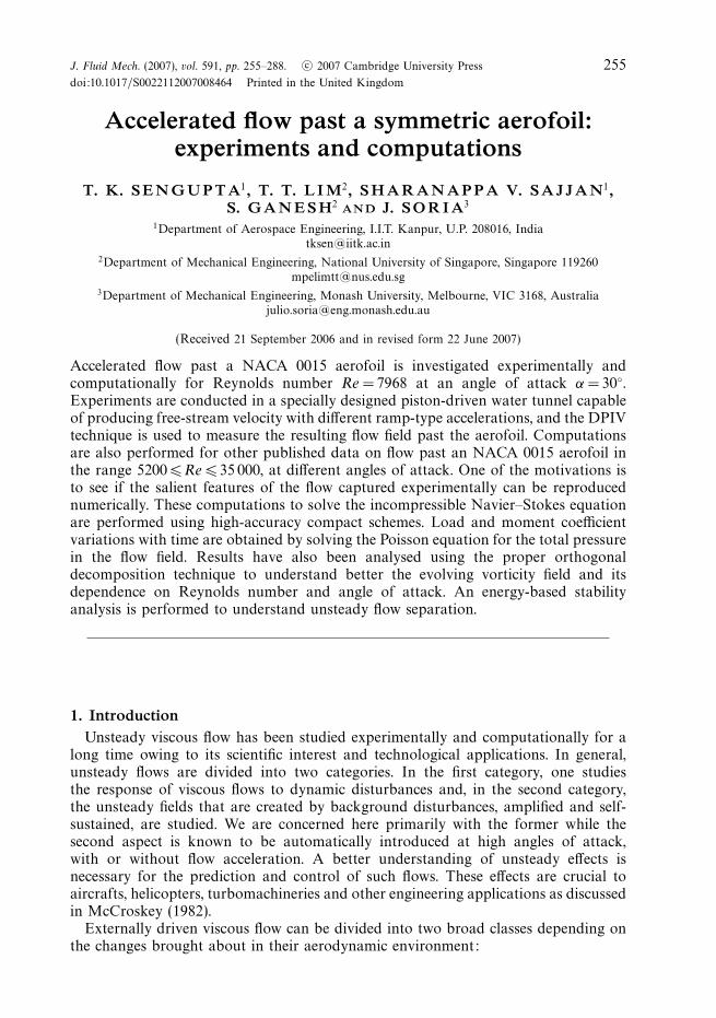
J. Fluid Mech. (2007), vol. 591, pp. 255–288. c© 2007 Cambridge University Press

doi:10.1017/S0022112007008464 Printed in the United Kingdom

255

Accelerated flow past a symmetric aerofoil:experiments and computations

T. K. SENGUPTA1, T. T. L IM2, SHARANAPPA V. SAJJAN1,S. GANESH2 AND J. SORIA3

1Department of Aerospace Engineering, I.I.T. Kanpur, U.P. 208016, [email protected]

2Department of Mechanical Engineering, National University of Singapore, Singapore [email protected]

3Department of Mechanical Engineering, Monash University, Melbourne, VIC 3168, [email protected]

(Received 21 September 2006 and in revised form 22 June 2007)

Accelerated flow past a NACA 0015 aerofoil is investigated experimentally andcomputationally for Reynolds number Re =7968 at an angle of attack α = 30◦.Experiments are conducted in a specially designed piston-driven water tunnel capableof producing free-stream velocity with different ramp-type accelerations, and the DPIVtechnique is used to measure the resulting flow field past the aerofoil. Computationsare also performed for other published data on flow past an NACA 0015 aerofoil inthe range 5200 � Re � 35 000, at different angles of attack. One of the motivations isto see if the salient features of the flow captured experimentally can be reproducednumerically. These computations to solve the incompressible Navier–Stokes equationare performed using high-accuracy compact schemes. Load and moment coefficientvariations with time are obtained by solving the Poisson equation for the total pressurein the flow field. Results have also been analysed using the proper orthogonaldecomposition technique to understand better the evolving vorticity field and itsdependence on Reynolds number and angle of attack. An energy-based stabilityanalysis is performed to understand unsteady flow separation.

1. IntroductionUnsteady viscous flow has been studied experimentally and computationally for a

long time owing to its scientific interest and technological applications. In general,unsteady flows are divided into two categories. In the first category, one studiesthe response of viscous flows to dynamic disturbances and, in the second category,the unsteady fields that are created by background disturbances, amplified and self-sustained, are studied. We are concerned here primarily with the former while thesecond aspect is known to be automatically introduced at high angles of attack,with or without flow acceleration. A better understanding of unsteady effects isnecessary for the prediction and control of such flows. These effects are crucial toaircrafts, helicopters, turbomachineries and other engineering applications as discussedin McCroskey (1982).

Externally driven viscous flow can be divided into two broad classes depending onthe changes brought about in their aerodynamic environment:

256 T. K. Sengupta, T. T. Lim, S. V. Sajjan, S. Ganesh and J. Soria

(i) when a body is moving in oscillating or plunging motion with a prescribedacceleration and

(ii) when a body is held fixed and the oncoming flow is allowed to change. e.g. asin translational acceleration or deceleration.

The case of translational acceleration is important as it relates to the flow establish-ment process in an experimental facility and in real-time applications, as in aero-dynamic decelerators. The acceleration and deceleration process can induce largetransient loads, limiting the performance and even leading to failure of the device. Inthis context, the most studied case is the impulsive start of the body. The reason behindthe assumption of impulsive motion is that in many practical applications this isadequate and, furthermore, it results in significant simplifications of the mathematicalformulations of the problem and can be used for validation of various numericalmethods. Early studies of typical impulsive viscous flow problems are due to Stokes(1851) and Rayleigh (1911) and involved obtaining the solution for an infinite flatplate started impulsively into motion in its own plane. Stuart (1963) and Schlichting(1979) have discussed another class of problems involving the establishment of free-stream speed with uniform acceleration. The problems of the boundary layer overa flat plate and circular cylinder with uniform acceleration were solved initially byBlasius and later extended by Gortler (see Schlichting 1979) for a general class ofnon-uniform acceleration. Collins & Dennis (1974) and Badr, Dennis & Kocabiyik(1996) have studied the symmetrical flow past accelerated circular cylinders. Theyobtained analytical and computational solutions of the Navier–Stokes equations inthe boundary layer coordinates using a perturbation series technique.

In numerical computations one often makes an implicit assumption that the long-time dynamics of the flow is independent of the initial start-up process. In Gendrich,Koochesfahani & Visbal (1995) and Koochesfahani & Smiljanovski (1993) it hasbeen shown that for a dynamically pitching aerofoil, the load and surface pressuredistribution on the aerofoil suction surface is affected only for a short time after theend of the initial acceleration period. Lugt & Haussling (1978) have studied the effectof acceleration on an ellipse of thickness to chord ratio (t/c) of 0.1 and concludedthat after the acceleration phase is over, differences in the flow characteristics amongvarious types of accelerations vanish rapidly. However, it should be noted that inboth Gendrich et al. (1995) and Lugt & Haussling (1978), the acceleration endedbefore leading-edge separation began. Sarpkaya (1991) has studied the effect ofuniform acceleration for flow past a circular cylinder. He defined a non-dimensionalacceleration parameter Ap given by

Ap = DdU∞

dt

/U 2

∞

where D is the cylinder diameter, U∞ is the final velocity and U∞ is the instantaneousvelocity. He noted that for Ap > 0.27, the drag coefficient beyond the period of initialacceleration does not measurably depend on Ap and the flow can be considered asimpulsively started. The drag overshoot and the relative displacement of the cylinderto reach this value remain more or less the same. For Ap < 0.27, the drag overshootreduces to its commonly accepted quasi-steady value as soon as the acceleration isremoved. However, Sarpkaya (1991) could not get repeatability of lift force for hisexperiments and stated that the lift force depends on initial disturbances that werenot maintainable during different experimental runs. Furthermore, he argued on thebasis of his experimental results that the manner in which acceleration is removedfrom the flow to sustain a constant velocity turned out to be more important than

Accelerated flow past a symmetric aerofoil 257

the manner in which the acceleration is imposed. For a dynamically pitching aerofoil,Choudhuri & Knight (1996), Currier & Fung (1992) and Carr & Chandrasekhara(1996) have noted that the compressibility is one of the major parameters affecting theflow. For the translational accelerations studied here, compressibility does not playa major role, as noted by comparing the peak suction values for the present casesto the results of Currier & Fung (1992). In the present work, we concentrate on theeffects of translational flow acceleration at low Reynolds numbers for incompressibleflow past aerofoils at high angles of attack.

One of the earliest computational works on the starting solution for flow pastan aerofoil is by Mehta & Lavan (1975) who studied the problem of laminar flowpast an impulsively started 9 % thick Joukowski aerofoil at Re = 1000. The flow pastthe aerofoil was seen to be dominated by the formation, growth and breakup ofseparation bubbles at this Reynolds number. Depending on the Reynolds numberand angle of attack, the unsteady separated flow may undergo laminar to turbulenttransition to form long or short bubbles. Whereas the short bubbles have only a smalleffect on the pressure distribution, the long bubbles result in a pressure distributionthat is different from the inviscid value. Ohmi et al. (1991) have presented someexperimental and computational results for a NACA 0012 aerofoil at 30◦ angleof attack for Re =3000. Nair & Sengupta (1998) have presented results for initialtimes with different start-up processes. Morikawa & Gronig (1995) have studied,experimentally and computationally, the unsteady aerodynamics of a NACA 0015aerofoil and provided a record of tunnel free-stream speed as a function of timefor the starting process. In the present study, we compute and compare with thisexperimental result for uniform flow past a NACA 0015 aerofoil at an angle of attackof 30◦ for Re = 35 000 for the given time history of the free-stream speed. A tangenthyperbolic representation was closest to the measured speed distribution in Morikawa& Gronig (1995) and is given by

U∞(t) = U∞ tanh

(t∗

τ ∗

)(1.1)

with U∞ the final steady tunnel speed and τ ∗ = 50 ms, as given in the reference.All calculations reported here are performed with times non-dimensionalized by theconvection time scale, constructed from U∞ and the chord of the aerofoil, and arerepresented by quantities without asterisks. For the numerical procedure followed inMorikawa & Gronig (1995), acceleration of the mean flow was accounted for by anadditional source term in the x-momentum equation derived from the time derivativeof (1.1). In an earlier experimental work, Freymuth (1985) studied the effect of uniformacceleration on flow past a NACA 0015 aerofoil at different Reynolds numbers andangles of attack by flow visualization. Note that in that work, the Reynolds numberwas defined in terms of the uniform acceleration and the chord of the aerofoil. Hisresults are reported for Reynolds number held constant, and thus by our conventionthe Reynolds number based on instantaneous convection speed will vary linearly withtime.

Here, we investigate constant acceleration cases (ramp-start) as shown in figure 3below. Zaman, McKinzie & Rumsey (1989) have shown, based on their experimentalresults, that the flow past aerofoils near stall can be two-dimensional. This is alsosupported in Lin & Pauley (1996), Huang & Lin (1995) and Brendal & Mueller (1988)for results obtained at early times after the flow start-up. In the present investigation,our focus is mainly on the flow onset process and the results obtained from the


solution of two-dimensional Navier–Stokes equation are considered adequate. Forflow over aerofoils near stall at high Reynolds numbers, the unsteadiness is largelydue to the low-frequency events of shed vortices and their convection.

A stream function–vorticity formulation is preferred for the computations herebecause the smaller number of unknowns compared to using primitive variablesmakes higher resolution calculations possible. Also, this formulation ensures exactsatisfaction of mass conservation, making a smaller demand on computationalrequirements than needed in the primitive variable formulation. Furthermore, ahigher accuracy is achieved by using compact schemes as developed and used inSengupta (2004) and Sengupta, Vikas & Johri (2005) for the discretization of nonlinearconvection terms of the vorticity transport equation. An orthogonal numerical gridgeneration technique developed in Nair & Sengupta (1998) is used here, which helpsto further reduce numerical error. In that work, some comparisons are made withthe results of Morikawa & Gronig (1995) for flow past a NACA 0015 aerofoil at aReynolds number of 35 000 and 30◦ angle of attack. The calculation was performedusing the same formulation, but with a third-order upwinding scheme.

In the present work, we further investigate the constant acceleration case experimen-tally for Re = 7968 and α = 30◦ for different acceleration parameters, and the detailsare given in § 2. In § 3, the formulation and the numerical methods used for thecomputations are given. The following cases are studied here, when flow acceleratesfrom zero velocity at t = 0:

A. A uniform acceleration case with Re = 7968, α =30◦ and τ =3.75 for which theexperimental results are provided in § 2.

B. A uniform flow with a tangent hyperbolic dependence of free-stream speed ontime for Re = 35 000, α = 30◦ and τ = 0.6. This case corresponds to the experimentsof Morikawa & Gronig (1995).

C. A uniform flow using a ramp start for Re = 35 000, α = 30◦ and τ = 0.5 to com-pare with the case B.

D. A uniform acceleration for Re = 5 200, α = 60◦ and 90◦ with very large τ . Thiscorresponds to the experiments of Freymuth (1985). The definition of the Reynoldsnumber for this case is given in § 4.3.

In § 4, computational and various experimental results are discussed case by case.In § 5, proper orthogonal decomposition of two cases is presented for different anglesof attack and Reynolds number to distinguish the flow structures at high angles ofattack. The paper concludes with a summary in § 6.

2. Experimental setup and proceduresThe experiments were conducted in a piston-driven closed-circuit water tunnel

in the Fluid Mechanics Laboratory of the National University of Singapore. Aschematic drawing of the tunnel is presented in figure 1. Unlike the conventional watertunnel with a continuous flow, this tunnel is driven by a square Plexiglas piston of198 mm × 198 mm, which pushes the water ahead of it as it slides along the testsection with the same dimensions. The piston is driven by a micro-stepper motor(Sanyo Denki, Model 103-8960-0140) via a ball and screw mechanism, which convertsthe rotational motion into a linear motion of the piston. The motor, which is poweredby a micro-steps driver (2D88M) and controlled by TTL signals generated by a Lab-view Program in a PC, can achieve 10 000 micro-steps per revolution or 0.036◦ perstep. With a pitch of the ball-screw of 25 mm, this translates into a linear resolution of3.125 × 10−4 mm per step. For safety reasons, the piston is confined to move between


Mirror

198 mmAirfoil Flow Piston

Steppermotor

Limit switches

Cylindricallens

Nd YagLaser

PC3 PC2 PC1

To PIVcamera

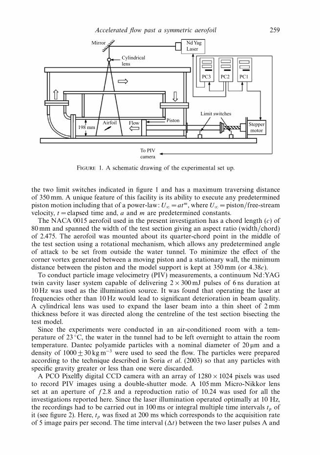
Figure 1. A schematic drawing of the experimental set up.

the two limit switches indicated in figure 1 and has a maximum traversing distanceof 350 mm. A unique feature of this facility is its ability to execute any predeterminedpiston motion including that of a power-law: U∞ = atm, where U∞ = piston/free-streamvelocity, t = elapsed time and, a and m are predetermined constants.

The NACA 0015 aerofoil used in the present investigation has a chord length (c) of80 mm and spanned the width of the test section giving an aspect ratio (width/chord)of 2.475. The aerofoil was mounted about its quarter-chord point in the middle ofthe test section using a rotational mechanism, which allows any predetermined angleof attack to be set from outside the water tunnel. To minimize the effect of thecorner vortex generated between a moving piston and a stationary wall, the minimumdistance between the piston and the model support is kept at 350 mm (or 4.38c).

To conduct particle image velocimetry (PIV) measurements, a continuum Nd:YAGtwin cavity laser system capable of delivering 2 × 300 mJ pulses of 6 ns duration at10 Hz was used as the illumination source. It was found that operating the laser atfrequencies other than 10 Hz would lead to significant deterioration in beam quality.A cylindrical lens was used to expand the laser beam into a thin sheet of 2 mmthickness before it was directed along the centreline of the test section bisecting thetest model.

Since the experiments were conducted in an air-conditioned room with a tem-perature of 23 ◦C, the water in the tunnel had to be left overnight to attain the roomtemperature. Dantec polyamide particles with a nominal diameter of 20 µm and adensity of 1000 ± 30 kg m−3 were used to seed the flow. The particles were preparedaccording to the technique described in Soria et al. (2003) so that any particles withspecific gravity greater or less than one were discarded.

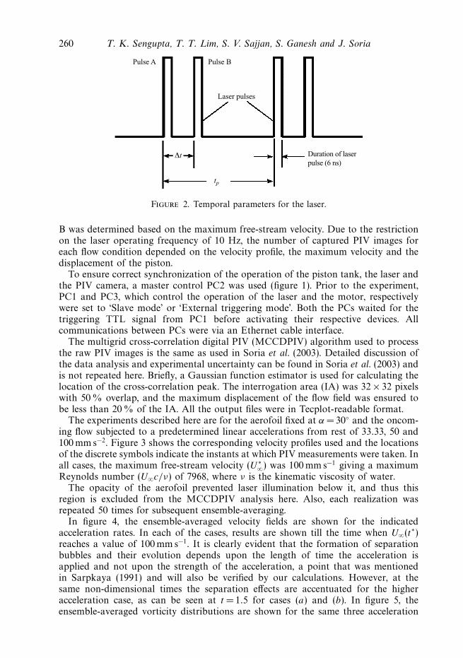
A PCO Pixelfly digital CCD camera with an array of 1280 × 1024 pixels was usedto record PIV images using a double-shutter mode. A 105 mm Micro-Nikkor lensset at an aperture of f 2.8 and a reproduction ratio of 10.24 was used for all theinvestigations reported here. Since the laser illumination operated optimally at 10 Hz,the recordings had to be carried out in 100 ms or integral multiple time intervals tp ofit (see figure 2). Here, tp was fixed at 200 ms which corresponds to the acquisition rateof 5 image pairs per second. The time interval (�t) between the two laser pulses A and


Pulse A Pulse B

Laser pulses

∆t

tp

Duration of laserpulse (6 ns)

Figure 2. Temporal parameters for the laser.

B was determined based on the maximum free-stream velocity. Due to the restrictionon the laser operating frequency of 10 Hz, the number of captured PIV images foreach flow condition depended on the velocity profile, the maximum velocity and thedisplacement of the piston.

To ensure correct synchronization of the operation of the piston tank, the laser andthe PIV camera, a master control PC2 was used (figure 1). Prior to the experiment,PC1 and PC3, which control the operation of the laser and the motor, respectivelywere set to ‘Slave mode’ or ‘External triggering mode’. Both the PCs waited for thetriggering TTL signal from PC1 before activating their respective devices. Allcommunications between PCs were via an Ethernet cable interface.

The multigrid cross-correlation digital PIV (MCCDPIV) algorithm used to processthe raw PIV images is the same as used in Soria et al. (2003). Detailed discussion ofthe data analysis and experimental uncertainty can be found in Soria et al. (2003) andis not repeated here. Briefly, a Gaussian function estimator is used for calculating thelocation of the cross-correlation peak. The interrogation area (IA) was 32 × 32 pixelswith 50 % overlap, and the maximum displacement of the flow field was ensured tobe less than 20 % of the IA. All the output files were in Tecplot-readable format.

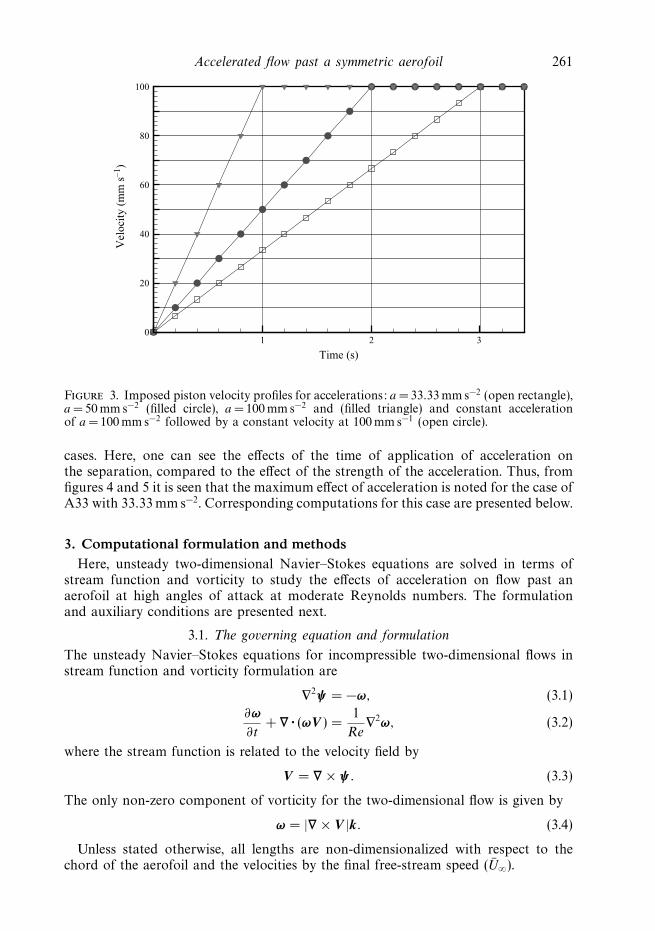
The experiments described here are for the aerofoil fixed at α = 30◦ and the oncom-ing flow subjected to a predetermined linear accelerations from rest of 33.33, 50 and100 mms−2. Figure 3 shows the corresponding velocity profiles used and the locationsof the discrete symbols indicate the instants at which PIV measurements were taken. Inall cases, the maximum free-stream velocity (U ∗

∞) was 100 mms−1 giving a maximumReynolds number (U∞c/ν) of 7968, where ν is the kinematic viscosity of water.

The opacity of the aerofoil prevented laser illumination below it, and thus thisregion is excluded from the MCCDPIV analysis here. Also, each realization wasrepeated 50 times for subsequent ensemble-averaging.

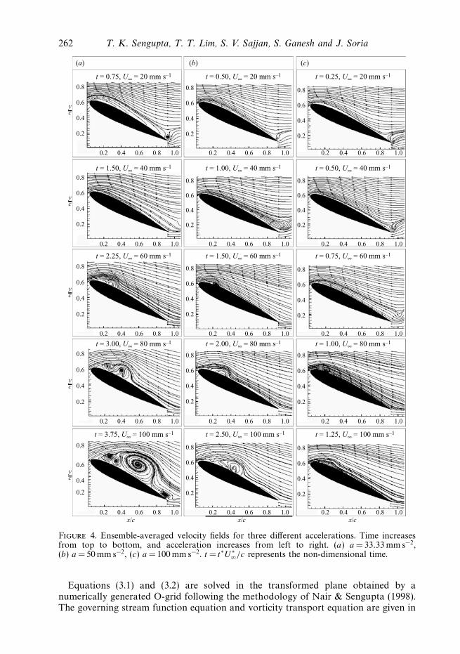
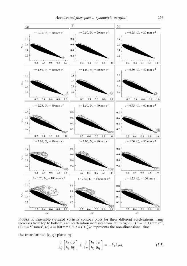
In figure 4, the ensemble-averaged velocity fields are shown for the indicatedacceleration rates. In each of the cases, results are shown till the time when U∞(t∗)reaches a value of 100 mms−1. It is clearly evident that the formation of separationbubbles and their evolution depends upon the length of time the acceleration isapplied and not upon the strength of the acceleration, a point that was mentionedin Sarpkaya (1991) and will also be verified by our calculations. However, at thesame non-dimensional times the separation effects are accentuated for the higheracceleration case, as can be seen at t = 1.5 for cases (a) and (b). In figure 5, theensemble-averaged vorticity distributions are shown for the same three acceleration


Time (s)

Vel

ocit

y (m

m s

–1)

1 2 30

20

40

60

80

100

Figure 3. Imposed piston velocity profiles for accelerations: a = 33.33mm s−2 (open rectangle),a = 50 mm s−2 (filled circle), a = 100mm s−2 and (filled triangle) and constant accelerationof a = 100 mm s−2 followed by a constant velocity at 100mm s−1 (open circle).

cases. Here, one can see the effects of the time of application of acceleration onthe separation, compared to the effect of the strength of the acceleration. Thus, fromfigures 4 and 5 it is seen that the maximum effect of acceleration is noted for the case ofA33 with 33.33 mms−2. Corresponding computations for this case are presented below.

3. Computational formulation and methodsHere, unsteady two-dimensional Navier–Stokes equations are solved in terms of

stream function and vorticity to study the effects of acceleration on flow past anaerofoil at high angles of attack at moderate Reynolds numbers. The formulationand auxiliary conditions are presented next.

3.1. The governing equation and formulation

The unsteady Navier–Stokes equations for incompressible two-dimensional flows instream function and vorticity formulation are

∇2ψ = −ω, (3.1)

∂ω

∂t+ ∇ · (ωV ) =

1

Re∇2ω, (3.2)

where the stream function is related to the velocity field by

V = ∇ × ψ . (3.3)

The only non-zero component of vorticity for the two-dimensional flow is given by

ω = |∇ × V |k. (3.4)

Unless stated otherwise, all lengths are non-dimensionalized with respect to thechord of the aerofoil and the velocities by the final free-stream speed (U∞).


t = 0.75, U∞ = 20 mm s–1 t = 0.50, U∞ = 20 mm s–1 t = 0.25, U∞ = 20 mm s–1





0.8

(a) (b) (c)

0.6

0.4

0.2

0.2 0.4 0.6 0.8 1.0 0.2 0.4 0.6 0.8 1.0 0.2 0.4 0.6 0.8 1.0

0.2 0.4 0.6 0.8 1.0 0.2 0.4 0.6 0.8 1.0 0.2 0.4 0.6 0.8 1.0

0.2 0.4 0.6 0.8 1.0 0.2 0.4 0.6 0.8 1.0 0.2 0.4 0.6 0.8 1.0

0.2 0.4 0.6 0.8 1.0 0.2 0.4 0.6 0.8 1.0 0.2 0.4 0.6 0.8 1.0

0.2 0.4 0.6x/c x/c x/c

0.8 1.0 0.2 0.4 0.6 0.8 1.0 0.2 0.4 0.6 0.8 1.0

0.8

0.6

0.4

0.2

0.8

0.6

0.4

0.2

0.8

0.6

0.4

0.2

0.8

0.6

0.4

0.2

0.8

0.6

0.4

0.2

0.8

0.6

0.4

0.2

0.8

0.6

0.4

0.2

0.8

0.6

0.4

0.2

0.8

0.6

0.4

0.2

0.8

0.6

0.4

0.2

0.8

0.6

0.4

0.2

0.8

0.6

0.4

0.2

0.8

0.6

0.4

0.2

0.8

0.6

0.4

0.2

yc

yc

yc

yc

yc

Figure 4. Ensemble-averaged velocity fields for three different accelerations. Time increasesfrom top to bottom, and acceleration increases from left to right. (a) a = 33.33 mm s−2,(b) a = 50 mm s−2, (c) a =100 mm s−2. t = t∗U ∗

∞/c represents the non-dimensional time.

Equations (3.1) and (3.2) are solved in the transformed plane obtained by anumerically generated O-grid following the methodology of Nair & Sengupta (1998).The governing stream function equation and vorticity transport equation are given in







0.8

(a) (b) (c)

0.6

0.4

0.2

0.2 0.4 0.6 0.8 1.0 0.2 0.4 0.6 0.8 1.0 0.2 0.4 0.6 0.8 1.0

0.2 0.4 0.6 0.8 1.0 0.2 0.4 0.6 0.8 1.0 0.2 0.4 0.6 0.8 1.0

0.2 0.4 0.6 0.8 1.0 0.2 0.4 0.6 0.8 1.0 0.2 0.4 0.6 0.8 1.0

0.2 0.4 0.6 0.8 1.0 0.2 0.4 0.6 0.8 1.0 0.2 0.4 0.6 0.8 1.0

0.2 0.4 0.6

x/c x/c x/c

0.8 1.0 0.2 0.4 0.6 0.8 1.0 0.2 0.4 0.6 0.8 1.0

0.8

0.6

0.4

0.2

0.8

0.6

0.4

0.2

0.8

0.6

0.4

0.2

0.8

0.6

0.4

0.2

0.8

0.6

0.4

0.2

0.8

0.6

0.4

0.2

0.8

0.6

0.4

0.2

0.8

0.6

0.4

0.2

0.8

0.6

0.4

0.2

0.8

0.6

0.4

0.2

0.8

0.6

0.4

0.2

0.8

0.6

0.4

0.2

0.8

0.6

0.4

0.2

0.8

0.6

0.4

0.2

yc

yc

yc

yc

yc

Figure 5. Ensemble-averaged vorticity contour plots for three different accelerations. Timeincreases from top to bottom, and acceleration increases from left to right. (a) a = 33.33 mm s−2,(b) a = 50 mm s2, (c) a = 100 mm s−2. t = t∗U ∗

∞/c represents the non-dimensional time.

the transformed (ξ, η)-plane by

∂

∂ξ

[h2

h1

∂ψ

∂ξ

]+

∂

∂η

[h1

h2

∂ψ

∂η

]= −h1h2ω, (3.5)


h1h2

∂ω

∂t+ h2u

∂ω

∂ξ+ h1v

∂ω

∂η=

1

Re

[∂

∂ξ

(h2

h1

∂ω

∂ξ

)+

∂

∂η

(h1

h2

∂ω

∂η

)], (3.6)

where h1 and h2 are scale factors of the transformation, given by h21 = (x2

ξ + y2ξ ) and

h22 = (x2

η + y2η).

In the transformed plane, the components of velocity are,

u =1

h2

∂ψ

∂η, v = − 1

h1

∂ψ

∂ξ. (3.7)

The stream function–vorticity formulation provides higher accuracy with respect toincompressibility assumption, but it does not yield the pressure field. Currier & Fung(1992) and Ramiz & Acharya (1992) have used experimental pressure coefficients tostudy unsteady separation. There is a need to accurately evaluate the pressure fieldbetter to understand unsteady flows since pressure fluctuations contain the signatureof coherent vortices located at the pressure trough. It has also been noted by Lesieur &Metais (1996) that low-pressure regions are better indicators of the coherent vorticesthan the high vorticity regions.

Thus, we solve the Poisson equation for the total pressure to obtain the pressurefield over the full computational domain. The governing Poisson equation for pressureis obtained by taking the divergence of the Navier–Stokes equation in primitivevariables. For an orthogonal curvilinear coordinate system, this is

∂

∂ξ

(h2

h1

∂P

∂ξ

)+

∂

∂η

(h1

h2

∂P

∂η

)=

∂

∂ξ(h2vω) − ∂

∂η(h1uω). (3.8)

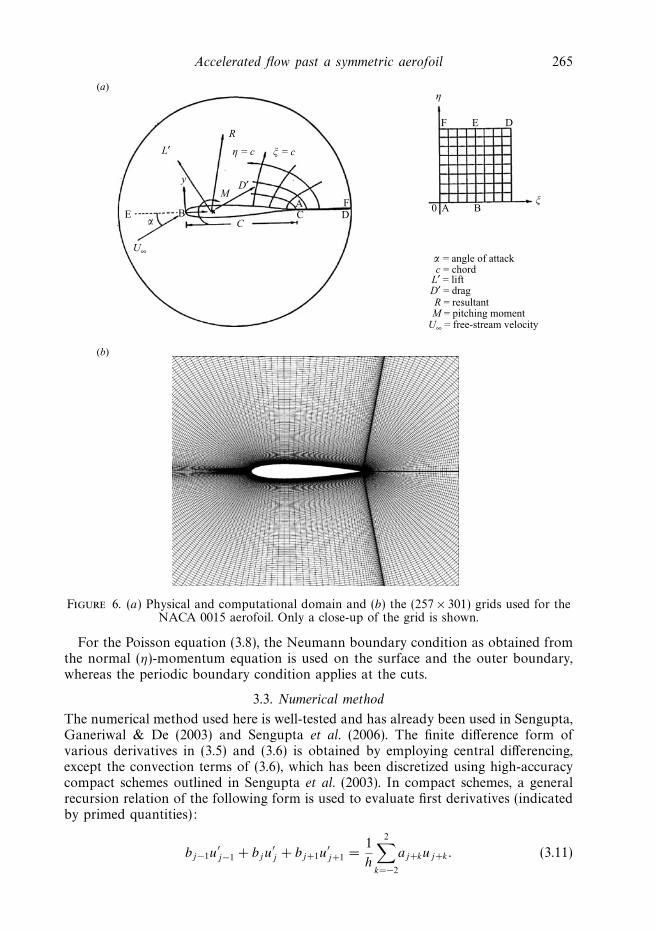
This formulation in an orthogonal grid was used earlier in Nair & Sengupta (1997a),which can be consulted for further details. The physical and computational domainsfor the present investigation are shown in figure 6(a). The numerically obtainedorthogonal grid is shown in figure 6(b). Note that a similar calculation for the effectof acceleration was reported in Nair & Sengupta (1997b), where a third-order upwindscheme (as given in Nair & Sengupta 1997a) was used with similar grids. In Senguptaet al. (2006), the same formulation has been used for flow past an aerofoil executingflapping and hovering motion using compact schemes. It is well known that compactschemes provide much higher resolution than explicit higher-order upwind schemes,thus enabling us to obtain numerical solutions with significantly enhanced accuracy.

3.2. Initial and boundary conditions

On the solid boundary ABC (in figure 6) the no-slip conditions apply,

ψ = constant,∂ψ

∂η= 0. (3.9)

These conditions also fix the wall vorticity, which is required as the boundarycondition for the vorticity transport equation. Periodic boundary conditions areapplied at the cuts (AF and CD) for all variables. For the stream function equation,at the outer boundary the Neumann boundary condition is used: ∂ψ/∂η = U∞∂y/∂η.To solve the vorticity transport equation, a fully developed condition is used as theboundary condition: ∂ω/∂η = 0. From equation (3.5), wall vorticity is calculated as

ω|body = − 1

h22

∂2ψ

∂η2

∣∣∣∣body

. (3.10)


L′

D′

ξ = cη = c

M

F

A0 B

E D

E

(a)

(b)

U∞

B

y

A FDC

C

R

α

η

ξ

α = angle of attackc = chord

L′ = liftD′ = dragR = resultantM = pitching moment

U∞ = free-stream velocity

Figure 6. (a) Physical and computational domain and (b) the (257 × 301) grids used for theNACA 0015 aerofoil. Only a close-up of the grid is shown.

For the Poisson equation (3.8), the Neumann boundary condition as obtained fromthe normal (η)-momentum equation is used on the surface and the outer boundary,whereas the periodic boundary condition applies at the cuts.

3.3. Numerical method

The numerical method used here is well-tested and has already been used in Sengupta,Ganeriwal & De (2003) and Sengupta et al. (2006). The finite difference form ofvarious derivatives in (3.5) and (3.6) is obtained by employing central differencing,except the convection terms of (3.6), which has been discretized using high-accuracycompact schemes outlined in Sengupta et al. (2003). In compact schemes, a generalrecursion relation of the following form is used to evaluate first derivatives (indicatedby primed quantities):

bj−1u′j−1 + bju

′j + bj+1u

′j+1 =

1

h

2∑k=−2

aj+kuj+k. (3.11)


In the periodic ξ -direction, the truncation error is minimized in the least-squaressense, by choosing the following coefficients in the above equation: bj±1 =0.3793894912, bj = 1, aj±1 = ± 0.7877868, aj±2 =±0.0458012 and aj = 0. The periodictridiagonal system obtained by the application of (3.11) for different nodes is solvedto evaluate the required ξ -derivatives in this direction.

In the non-periodic η-direction, one cannot apply the stencil (3.11) for all the nodes.For example, stable boundary closure schemes are required for the first and secondnode. The ones used are given by

u′1 =

(−3u1 + 4u2 − u3)

2h, (3.12)

u′2 =

[(2β2

3− 1

3

)u1 −

(8β2

3+

1

2

)u2 + (4β2 + 1)u3 −

(8β2

3+

1

6

)u4 +

2β2

3u5

]/h,

(3.13)

with β2 as a parameter to be chosen to ensure accuracy and stability. Similarly,boundary closure schemes are used for j = (N −1) and j = N with another parameter,βN−1. For the boundary closure, we have used β2 = −0.09 and βN−1 = 0.09. Applicationof (3.11) and the boundary closure schemes for different nodes in the η-direction leadsto a tridiagonal system that can be solved to obtain the derivatives with respect toη for the vorticity. To numerically stabilize the computations, an explicit fourthdissipation term is added to the calculated first derivatives (see Sengupta et al. 2006for further details).

4. Results and discussionThe orthogonal grids of size (257 × 301) were generated for the aerofoil by the

procedure developed in Nair & Sengupta (1998) and shown in figure 6(b), for fewrepresentative grid lines close to the aerofoil. The grid generation method is basedon the solution of the Beltrami equation, a hyperbolic partial differential equation oforder two, in which, starting from the aerofoil surface, constant-η lines are generatedby marching outwards with prescribed grid spacing in the hyperbolic direction. Thisability to prescribe the spacing in the normal direction is an added advantage ofthe grid generation method used and helps to provide adequate resolution in thewall-normal direction and in the wake region. Also, the spacing in the normaldirection is chosen in such a way that the truncation error does not give rise tospurious dispersion and dissipation. This is one of the important aspects of thepresent solution methodology. The outer boundary is located 12 chords away fromthe body. The present orthogonal grid needs fewer terms to be discretized than anon-orthogonal grid, which reduces the sources of truncation error. For the resultspresented here, a grid spacing of 0.00001c was used in the direction normal to theaerofoil surface.

The time integration of VTE uses a time step of �t = 0.00001 for the calculationspresented. The choice of the time step was dictated by the required accuracy and toavoid numerical instability for the explicit four-stage Runge–Kutta method used. Also,it should be noted that the loads are obtained by the vorticity values and the pressurevalues on the surface obtained by solving the pressure Poisson equation. One of theadvantages of the present method is that the pressure field can be calculated off-line,which increases the speed of the overall computations. As noted earlier, the purposeof the computation is to aid in understanding the effects of different levels and typesof acceleration on the growth and shedding of vortices. Before discussing these, it


is necessary to introduce some general terminologies used in this section. A surfacebubble is considered closed if it is completely enclosed by the body streamline. Addi-tional closed streamline loops can also be present inside an enclosed bubble, and theircentres are different from the centre of the enclosed bubble. Bubbles are defined asclockwise or anticlockwise depending on the direction of the velocity vector associatedwith the closed streamline inside them. Similarly a vortex is represented by a closedequivorticity line. Perry, Chong & Lim (1982) provide a descriptive understanding ofnear-wake vortex formation, and have used the term alleyway to describe the vortexshedding phenomena by examining instantaneous streamlines. Alleyway refers to aninstantaneous passage in the near-wake region where the streamlines upstream donot begin or end at critical points (i.e. points where all velocity components are zero).

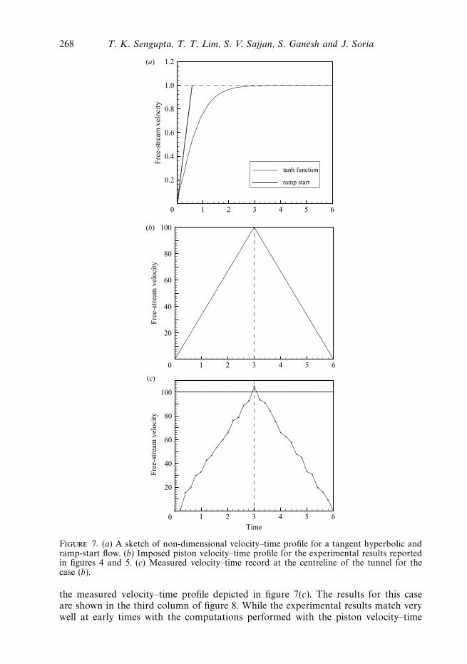
Some preliminary results were presented by Nair & Sengupta (1997b, 1998) andcompared their simulations with the corresponding experimental results at differentRe. For a truly impulsive start, the conditions at t = 0 should correspond to that ofan inviscid flow. Different types of flow start-up that are studied here are shown infigures 7(a) and 7(b). In figure 7(a), two different approaches to achieve the same finalvelocity are presented: the first one is that used in Morikawa & Gronig (1995) andgiven by equation (1.1); the second is the case of a ramp-start that takes the flowfrom zero to the final velocity by a uniform acceleration. In figure 7(b), the pistonvelocity–time profile used in the present experiment and computation is presentedfor the A33 case. In the experiments, a constant accelerated start is followed by aconstant deceleration, so that the flow velocity is zero after 6 s. In all the experiments,the maximum velocity attained is 100 mm s−1 and computations are performed hereonly for the case a = 33.33 mms−2. While the velocity shown in figure 7(b) correspondsto the piston velocity, we have also measured the actual flow velocity at the centrelineof the tunnel, and the velocity–time record is shown in figure 7(c). Note that thekinks in the velocity profile in figure 7(c) are caused by an uneven expansion of thesquare Plexiglas piston tank when filled with water. In air, the piston slides smoothlyalong the walls of the tank, but with water, the uneven absorption of the water bythe Plexiglas wall plus the weight of the water distorts the test section slightly fromits original square shape. Attempts were made to rectify the problem by trimmingthe dimension of the piston to match that of the tank, but the size of the pistoncould not be reduced too much, otherwise the mismatch would cause the flow toleak through the gaps between the piston and the tank. Despite the unavoidableproblem, the velocity distribution (in an average sense) still displays a reasonable‘constant’ acceleration and deceleration. The occurrence of the kinks equidistant intime is due to the DPIV system which only allows velocity measurements at discretetime intervals. We have performed computations for both the cases depicted in figures7(b) and 7(c) and compared them to understand the role of the small variation inacceleration seen in figure 7(c). Next we present results for different cases identifiedat the end of § 1 as Cases A to D.

4.1. Case A

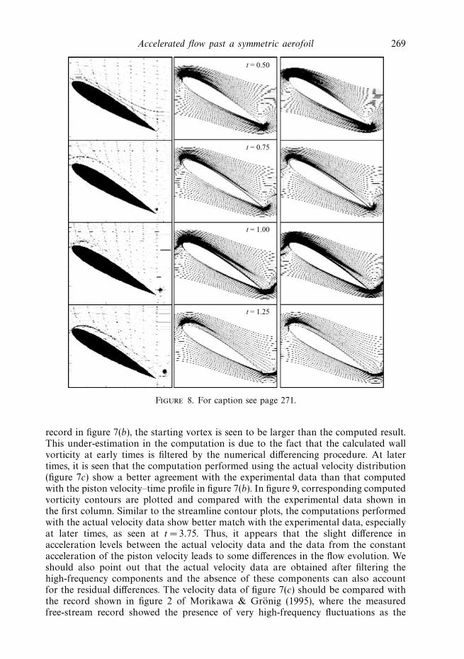
In this case, the acceleration of flow from zero to a final velocity of 100 mm s−1 wasachieved in 3 s via a uniform acceleration, and the corresponding results are shownin figures 4 and 5 (case a). Experimentally obtained instantaneous integral curvesgenerated from the instantaneous velocity field are compared with the computedstreamline contours obtained up to t = 3.75 (non-dimensional time) in figure 8 forthe piston velocity–time profile shown in figure 7(b). These two sets of results areshown in the first and middle columns of figure 8. Another case is computed using


Fre

e-st

ream

vel

ocit

y

0 1 2 3 4 5 6

0.2

0.4

0.6

0.8

1.0

1.2

tanh function

ramp start

(a)

Fre

e-st

ream

vel

ocit

y

0 1 2 3 4 5 6

20

40

60

80

100(b)

Time

Fre

e-st

ream

vel

ocit

y

0 1 2 3 4 5 6

20

40

60

80

100

(c)

Figure 7. (a) A sketch of non-dimensional velocity–time profile for a tangent hyperbolic andramp-start flow. (b) Imposed piston velocity–time profile for the experimental results reportedin figures 4 and 5. (c) Measured velocity–time record at the centreline of the tunnel for thecase (b).

the measured velocity–time profile depicted in figure 7(c). The results for this caseare shown in the third column of figure 8. While the experimental results match verywell at early times with the computations performed with the piston velocity–time


t = 0.50

t = 0.75

t = 1.00

t = 1.25

Figure 8. For caption see page 271.

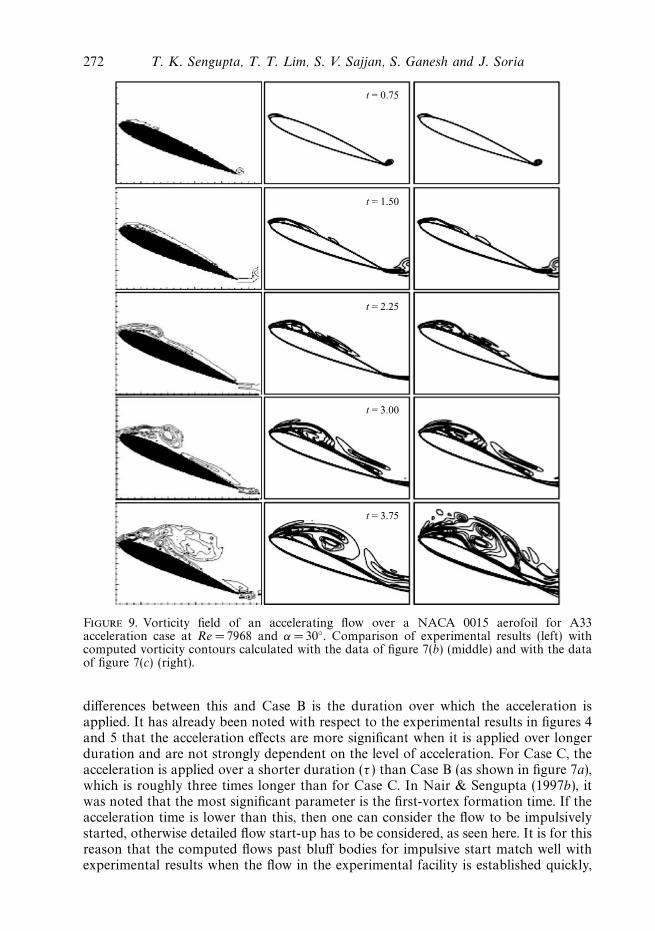
record in figure 7(b), the starting vortex is seen to be larger than the computed result.This under-estimation in the computation is due to the fact that the calculated wallvorticity at early times is filtered by the numerical differencing procedure. At latertimes, it is seen that the computation performed using the actual velocity distribution(figure 7c) show a better agreement with the experimental data than that computedwith the piston velocity–time profile in figure 7(b). In figure 9, corresponding computedvorticity contours are plotted and compared with the experimental data shown inthe first column. Similar to the streamline contour plots, the computations performedwith the actual velocity data show better match with the experimental data, especiallyat later times, as seen at t = 3.75. Thus, it appears that the slight difference inacceleration levels between the actual velocity data and the data from the constantacceleration of the piston velocity leads to some differences in the flow evolution. Weshould also point out that the actual velocity data are obtained after filtering thehigh-frequency components and the absence of these components can also accountfor the residual differences. The velocity data of figure 7(c) should be compared withthe record shown in figure 2 of Morikawa & Gronig (1995), where the measuredfree-stream record showed the presence of very high-frequency fluctuations as the


t = 1.50

t = 1.75

t = 2.00

t = 2.50

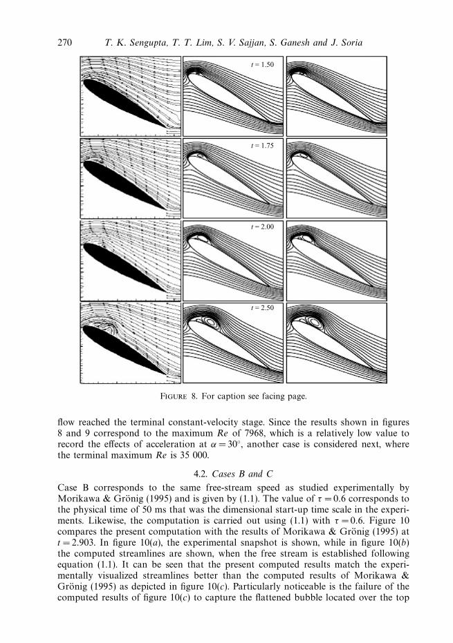
Figure 8. For caption see facing page.

flow reached the terminal constant-velocity stage. Since the results shown in figures8 and 9 correspond to the maximum Re of 7968, which is a relatively low value torecord the effects of acceleration at α =30◦, another case is considered next, wherethe terminal maximum Re is 35 000.

4.2. Cases B and C

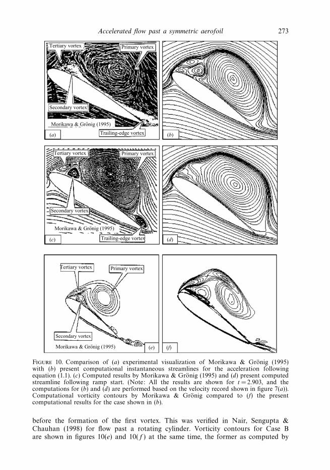
Case B corresponds to the same free-stream speed as studied experimentally byMorikawa & Gronig (1995) and is given by (1.1). The value of τ = 0.6 corresponds tothe physical time of 50 ms that was the dimensional start-up time scale in the experi-ments. Likewise, the computation is carried out using (1.1) with τ = 0.6. Figure 10compares the present computation with the results of Morikawa & Gronig (1995) att = 2.903. In figure 10(a), the experimental snapshot is shown, while in figure 10(b)the computed streamlines are shown, when the free stream is established followingequation (1.1). It can be seen that the present computed results match the experi-mentally visualized streamlines better than the computed results of Morikawa &Gronig (1995) as depicted in figure 10(c). Particularly noticeable is the failure of thecomputed results of figure 10(c) to capture the flattened bubble located over the top


t = 2.75

t = 3.00

t = 3.50

t = 3.75

Figure 8. Flow field of an accelerating flow over a NACA 0015 aerofoil for A33 accelerationcase at Re = 7968 and α = 30◦. Comparison of experimental results (left) with computedstreamline contours calculated with the data of figure 7(b) (middle) and with the data offigure 7(c) (right) from t = 0.5 to t = 3.75.

surface of the aerofoil in the experimental results. In contrast, this feature of theseparation bubble is clearly seen in figure 10(b). As discussed in Nair & Sengupta(1997b, 1998), the computational results of figure 10(c) resemble a case computedby the present method using the free-stream speed established by an impulsive startcondition. The distorted primary bubble with flattened top is captured by followingthe correct free-stream speed variation, thus emphasizing the need to correctly specifythe start-up process.

To show this sensitivity to the start-up process, we have performed anothercalculation (Case C) where the final free-stream speed is achieved following a rampstart, i.e. the flow starts from zero velocity and reaches the terminal speed at t = τ .Computed streamlines are shown in figure 10(d), and it is evident that the separationbubble for this case is under-developed compared to that in figure 10(b). Also, thesecondary and tertiary vortices are either significantly weaker or not visible, whilethe primary bubble covers and extends beyond the top surface. The reason for the


t = 0.75

t = 1.50

t = 2.25

t = 3.00

t = 3.75

Figure 9. Vorticity field of an accelerating flow over a NACA 0015 aerofoil for A33acceleration case at Re = 7968 and α = 30◦. Comparison of experimental results (left) withcomputed vorticity contours calculated with the data of figure 7(b) (middle) and with the dataof figure 7(c) (right).

differences between this and Case B is the duration over which the acceleration isapplied. It has already been noted with respect to the experimental results in figures 4and 5 that the acceleration effects are more significant when it is applied over longerduration and are not strongly dependent on the level of acceleration. For Case C, theacceleration is applied over a shorter duration (τ ) than Case B (as shown in figure 7a),which is roughly three times longer than for Case C. In Nair & Sengupta (1997b), itwas noted that the most significant parameter is the first-vortex formation time. If theacceleration time is lower than this, then one can consider the flow to be impulsivelystarted, otherwise detailed flow start-up has to be considered, as seen here. It is for thisreason that the computed flows past bluff bodies for impulsive start match well withexperimental results when the flow in the experimental facility is established quickly,


Tertiary vortex Primary vortex



Secondary vortex

Secondary vortex

Secondary vortex

Trailing-edge vortex

Morikawa & Gronig (1995)¨

(a)

Trailing-edge vortex(c) (d)

(e) (f)

(b)



Figure 10. Comparison of (a) experimental visualization of Morikawa & Gronig (1995)with (b) present computational instantaneous streamlines for the acceleration followingequation (1.1). (c) Computed results by Morikawa & Gronig (1995) and (d) present computedstreamline following ramp start. (Note: All the results are shown for t = 2.903, and thecomputations for (b) and (d) are performed based on the velocity record shown in figure 7(a)).Computational vorticity contours by Morikawa & Gronig compared to (f) the presentcomputational results for the case shown in (b).

before the formation of the first vortex. This was verified in Nair, Sengupta &Chauhan (1998) for flow past a rotating cylinder. Vorticity contours for Case Bare shown in figures 10(e) and 10(f ) at the same time, the former as computed by


Cl

0 5 10 15 20 25 30 35 40 45 50

0 5 10 15 20 25 30 35 40 45 50

0 5 10 15 20 25 30 35 40 45 50

–60

–40

–20

0

20

Cd

–40

–20

0

20

CMle

–40

–20

0

20

Time

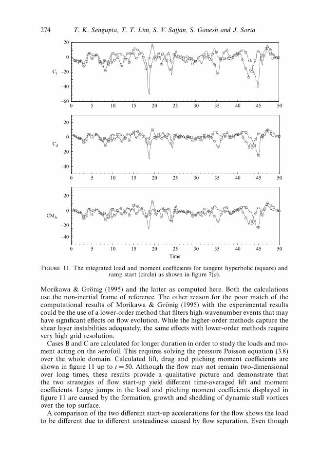
Figure 11. The integrated load and moment coefficients for tangent hyperbolic (square) andramp start (circle) as shown in figure 7(a).

Morikawa & Gronig (1995) and the latter as computed here. Both the calculationsuse the non-inertial frame of reference. The other reason for the poor match of thecomputational results of Morikawa & Gronig (1995) with the experimental resultscould be the use of a lower-order method that filters high-wavenumber events that mayhave significant effects on flow evolution. While the higher-order methods capture theshear layer instabilities adequately, the same effects with lower-order methods requirevery high grid resolution.

Cases B and C are calculated for longer duration in order to study the loads and mo-ment acting on the aerofoil. This requires solving the pressure Poisson equation (3.8)over the whole domain. Calculated lift, drag and pitching moment coefficients areshown in figure 11 up to t =50. Although the flow may not remain two-dimensionalover long times, these results provide a qualitative picture and demonstrate thatthe two strategies of flow start-up yield different time-averaged lift and momentcoefficients. Large jumps in the load and pitching moment coefficients displayed infigure 11 are caused by the formation, growth and shedding of dynamic stall vorticesover the top surface.

A comparison of the two different start-up accelerations for the flow shows the loadto be different due to different unsteadiness caused by flow separation. Even though


the loads for the two cases do not follow the same curve as in Lugt & Haussling(1978) and Gendrich et al. (1995), they have the same order of magnitude and followsimilar trends. In Lugt & Haussling (1978) and Gendrich et al. (1995), accelerationwas completed by time t = 0.25, which is before the formation of the first leading-edgebubble. Sarpkaya (1991) also obtained a similar trend for drag, following the samecurve for the case where the acceleration parameter Ap was greater than 0.27. For allother cases where Ap < 0.27, the drag reached a quasi-steady state. In contrast, theleading-edge vortices observed here are already formed before the acceleration phaseis completed and the detailed load variation depends on the formation time of thefirst vortex and subsequent instabilities of the separated shear layer.

In both cases, there is little interaction between vortices shed from leading andtrailing edges at this Reynolds number and the angle of attack of the aerofoil, as alsonoted in Huang & Lin (1995). The vortex shedding is predominantly from the leadingedge only, and is different from the Karman vortex streets behind bluff bodies. Forthe lower Reynolds number case shown in figure 8, the shear layer separated fromthe leading edge does not shed clearly and interacts with the separated shear layerfrom the trailing edge, causing slow time variation of physical variables in the wake.Such an interacting leading-edge laminar separation bubble was also noted by Lin &Pauley (1996), Zaman et al. (1989) and Sugavanam & Wu (1982). They concludedthat the low-frequency oscillation over the aerofoil is due to the vortex shedding fromlaminar separation bubbles.

Similarly, comparing the present computations for flow past an aerofoil to that forellipses in Nair & Sengupta (1997a), it is noticed that the leading-edge stagnationpoint does not move for the aerofoil at post-stall angles of attack of 30◦. Also, the rearstagnation point is always near the trailing edge except when alleyways are formed.This is due to the presence of the sharp trailing edge and the resultant interactionsof vortices in the wake are relatively weaker for aerofoils than to ellipses.

4.3. Case D

This case corresponds to the experimental results reported in Freymuth (1985) for theuniform acceleration case at significantly higher angles of attack, while the maximumReynolds number is fixed at 5200. This particular case of uniform acceleration has ahigher acceleration level, with τ much larger than for the previous cases. Of all theexperimental cases in Freymuth (1985), 60◦ and 90◦ angle of attack cases are computedbecause of the stronger vortical structures seen in the experimental visualizations, andsuch cases have not been computed before. For the flow visualization in Freymuth(1985), liquid titanium tetrachloride (TiCl4) is applied on the aerofoil surface, andthe ‘smoke’ produced by the evaporation of the injected liquid is accumulated in thelow-velocity recirculation zone. It is therefore difficult to give a proper interpretationof the visualization pictures. These are in a strict sense not streaklines as the amountof liquid injected is so large that the ‘smoke’ does not emanate from a single point.The visualization pictures reveal a combination of high-stress and low-convectionpockets. Thus, the pictures can be compared qualitatively with vorticity and pressurecontours. Also, due to the slightly reflective surface of the aerofoil, a mirror image ofthe detected structures is also captured in the visualization pictures.

4.3.1. Cases of α =60◦ and 90◦ for Re = 5200

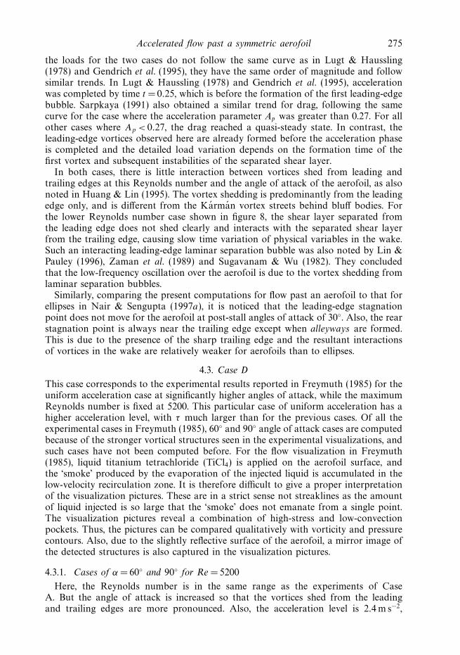
Here, the Reynolds number is in the same range as the experiments of CaseA. But the angle of attack is increased so that the vortices shed from the leadingand trailing edges are more pronounced. Also, the acceleration level is 2.4 m s−2,


t = 1.49

t = 1.60

t = 2.10

t = 2.40

Figure 12. For caption see facing page.

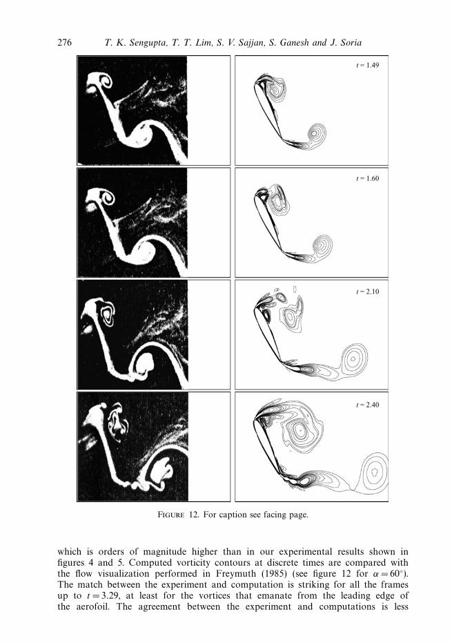
which is orders of magnitude higher than in our experimental results shown infigures 4 and 5. Computed vorticity contours at discrete times are compared withthe flow visualization performed in Freymuth (1985) (see figure 12 for α = 60◦).The match between the experiment and computation is striking for all the framesup to t = 3.29, at least for the vortices that emanate from the leading edge ofthe aerofoil. The agreement between the experiment and computations is less


t = 2.73

t = 3.16

t = 3.29

t = 3.84

Figure 12. Comparison of present vorticity contours (right) with visualization pictures (left)from Freymuth (1985) for Re =5200 and α = 60◦ and time increasing from t = 1.49 to t = 3.84.

satisfactory for the vortical structures released from the trailing edge of the aerofoil.While two-dimensional calculations are capable of capturing vortices created by thecombined action of local flow acceleration followed by rapid deceleration near theleading edge, vortices emerging from the trailing edge show a tendency of mergingin a two-dimensional simulation, as noted in Lesieur & Metais (1996). This so-calledbackscatter problem was discussed in Mathaeus et al. (1991) and Brachet et al.


t = 1.49 t = 2.73

t = 1.60 t = 3.16

t = 2.10 t = 3.29

t = 2.40 t = 3.84

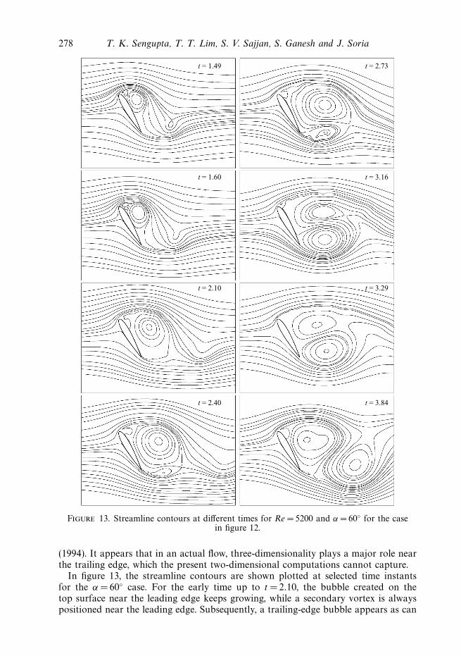
Figure 13. Streamline contours at different times for Re =5200 and α =60◦ for the casein figure 12.

(1994). It appears that in an actual flow, three-dimensionality plays a major role nearthe trailing edge, which the present two-dimensional computations cannot capture.

In figure 13, the streamline contours are shown plotted at selected time instantsfor the α = 60◦ case. For the early time up to t = 2.10, the bubble created on thetop surface near the leading edge keeps growing, while a secondary vortex is alwayspositioned near the leading edge. Subsequently, a trailing-edge bubble appears as can


t = 1.49

t = 1.60 t = 3.16

t = 2.10 t = 3.29

t = 2.40 t = 3.84

t = 2.73

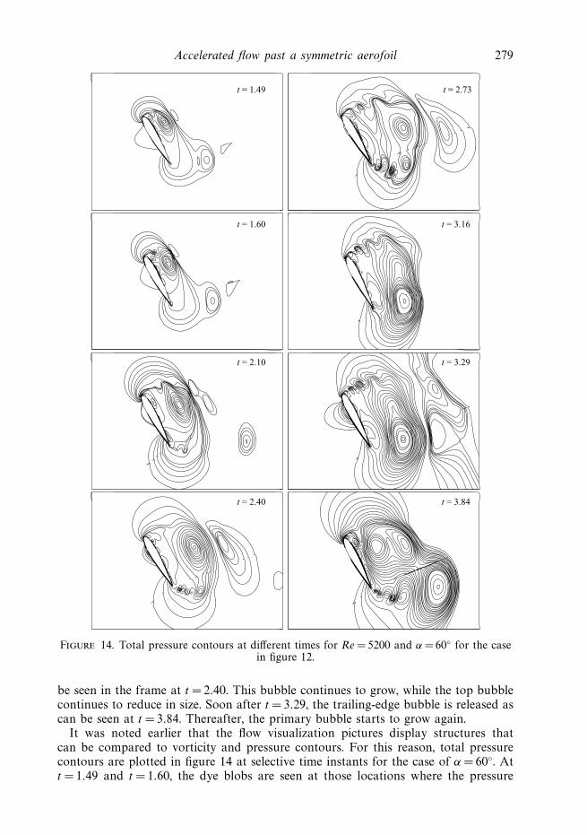
Figure 14. Total pressure contours at different times for Re = 5200 and α = 60◦ for the casein figure 12.

be seen in the frame at t = 2.40. This bubble continues to grow, while the top bubblecontinues to reduce in size. Soon after t = 3.29, the trailing-edge bubble is released ascan be seen at t =3.84. Thereafter, the primary bubble starts to grow again.

It was noted earlier that the flow visualization pictures display structures thatcan be compared to vorticity and pressure contours. For this reason, total pressurecontours are plotted in figure 14 at selective time instants for the case of α = 60◦. Att = 1.49 and t =1.60, the dye blobs are seen at those locations where the pressure


t = 0.93

t = 1.92

t = 2.42

t = 2.92

t = 3.42

t = 3.90

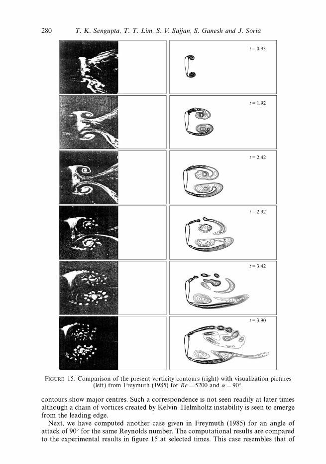
Figure 15. Comparison of the present vorticity contours (right) with visualization pictures(left) from Freymuth (1985) for Re =5200 and α = 90◦.

contours show major centres. Such a correspondence is not seen readily at later timesalthough a chain of vortices created by Kelvin–Helmholtz instability is seen to emergefrom the leading edge.

Next, we have computed another case given in Freymuth (1985) for an angle ofattack of 90◦ for the same Reynolds number. The computational results are comparedto the experimental results in figure 15 at selected times. This case resembles that of


t = 0.93 t = 2.92

t = 1.92 t = 3.42

t = 2.42 t = 3.90

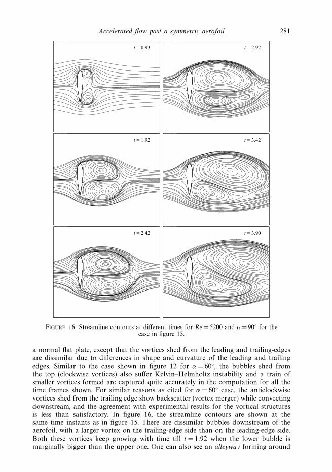
Figure 16. Streamline contours at different times for Re = 5200 and α = 90◦ for thecase in figure 15.

a normal flat plate, except that the vortices shed from the leading and trailing-edgesare dissimilar due to differences in shape and curvature of the leading and trailingedges. Similar to the case shown in figure 12 for α = 60◦, the bubbles shed fromthe top (clockwise vortices) also suffer Kelvin–Helmholtz instability and a train ofsmaller vortices formed are captured quite accurately in the computation for all thetime frames shown. For similar reasons as cited for α = 60◦ case, the anticlockwisevortices shed from the trailing edge show backscatter (vortex merger) while convectingdownstream, and the agreement with experimental results for the vortical structuresis less than satisfactory. In figure 16, the streamline contours are shown at thesame time instants as in figure 15. There are dissimilar bubbles downstream of theaerofoil, with a larger vortex on the trailing-edge side than on the leading-edge side.Both these vortices keep growing with time till t = 1.92 when the lower bubble ismarginally bigger than the upper one. One can also see an alleyway forming around


Number of modes

Ens

trop

hy c

onte

nt

5 10 15 20 25 30 35 40

0.6

0.7

0.8

0.9

1.0

α = 30°

α = 60°

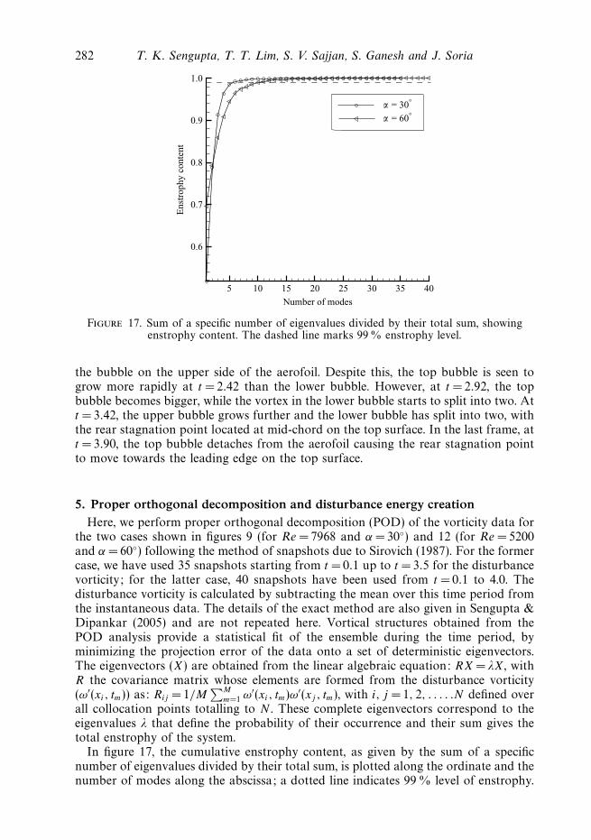
Figure 17. Sum of a specific number of eigenvalues divided by their total sum, showingenstrophy content. The dashed line marks 99 % enstrophy level.

the bubble on the upper side of the aerofoil. Despite this, the top bubble is seen togrow more rapidly at t =2.42 than the lower bubble. However, at t =2.92, the topbubble becomes bigger, while the vortex in the lower bubble starts to split into two. Att = 3.42, the upper bubble grows further and the lower bubble has split into two, withthe rear stagnation point located at mid-chord on the top surface. In the last frame, att = 3.90, the top bubble detaches from the aerofoil causing the rear stagnation pointto move towards the leading edge on the top surface.

5. Proper orthogonal decomposition and disturbance energy creationHere, we perform proper orthogonal decomposition (POD) of the vorticity data for

the two cases shown in figures 9 (for Re = 7968 and α = 30◦) and 12 (for Re = 5200and α = 60◦) following the method of snapshots due to Sirovich (1987). For the formercase, we have used 35 snapshots starting from t = 0.1 up to t = 3.5 for the disturbancevorticity; for the latter case, 40 snapshots have been used from t = 0.1 to 4.0. Thedisturbance vorticity is calculated by subtracting the mean over this time period fromthe instantaneous data. The details of the exact method are also given in Sengupta &Dipankar (2005) and are not repeated here. Vortical structures obtained from thePOD analysis provide a statistical fit of the ensemble during the time period, byminimizing the projection error of the data onto a set of deterministic eigenvectors.The eigenvectors (X) are obtained from the linear algebraic equation: RX = λX, withR the covariance matrix whose elements are formed from the disturbance vorticity(ω′(xi, tm)) as: Rij = 1/M

∑M

m=1 ω′(xi, tm)ω′(xj , tm), with i, j = 1, 2, . . . . .N defined overall collocation points totalling to N . These complete eigenvectors correspond to theeigenvalues λ that define the probability of their occurrence and their sum gives thetotal enstrophy of the system.

In figure 17, the cumulative enstrophy content, as given by the sum of a specificnumber of eigenvalues divided by their total sum, is plotted along the ordinate and thenumber of modes along the abscissa; a dotted line indicates 99 % level of enstrophy.


1

0y

–1

–20 1 2 3 4

Eigen vector 1

5 6 7 8

1

0y

–1

–20 1 2 3 4

Eigen vector 2

Eigen vector 3

5 6 7 8

1

0y

–1

–1.5

–20 1 2 3 4

x5 6 7 8

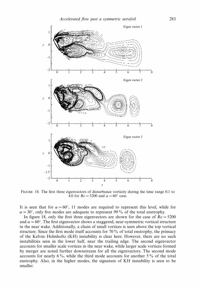
Figure 18. The first three eigenvectors of disturbunce vorticity during the time range 0.1 to4.0 for Re =5200 and α =60◦ case.

It is seen that for α =60◦, 11 modes are required to represent this level, while forα = 30◦, only five modes are adequate to represent 99 % of the total enstrophy.

In figure 18, only the first three eigenvectors are shown for the case of Re = 5200and α = 60◦. The first eigenvector shows a staggered, near-symmetric vortical structurein the near wake. Additionally, a chain of small vortices is seen above the top vorticalstructure. Since the first mode itself accounts for 70 % of total enstrophy, the primacyof the Kelvin–Helmholtz (KH) instability is clear here. However, there are no suchinstabilities seen in the lower half, near the trailing edge. The second eigenvectoraccounts for smaller scale vortices in the near wake, while larger scale vortices formedby merger are noted further downstream for all the eigenvectors. The second modeaccounts for nearly 6 %, while the third mode accounts for another 5 % of the totalenstrophy. Also, in the higher modes, the signature of KH instability is seen to besmaller.


0.4

0.2

0

y–0.2

–0.4

–0.6

–0.8

0 0.5 1

1

Eigenvector 1

1.5 2 2.5 3

0.4

0.2

0

y–0.2

–0.4

–0.6

–0.8

0 0.5

Eigenvector 2

1.5 2 2.5 3

1

0.4

0.2

0

y–0.2

–0.4

–0.6

–0.8

0 0.5

Eigenvector 3

1.5x

2 2.5 3

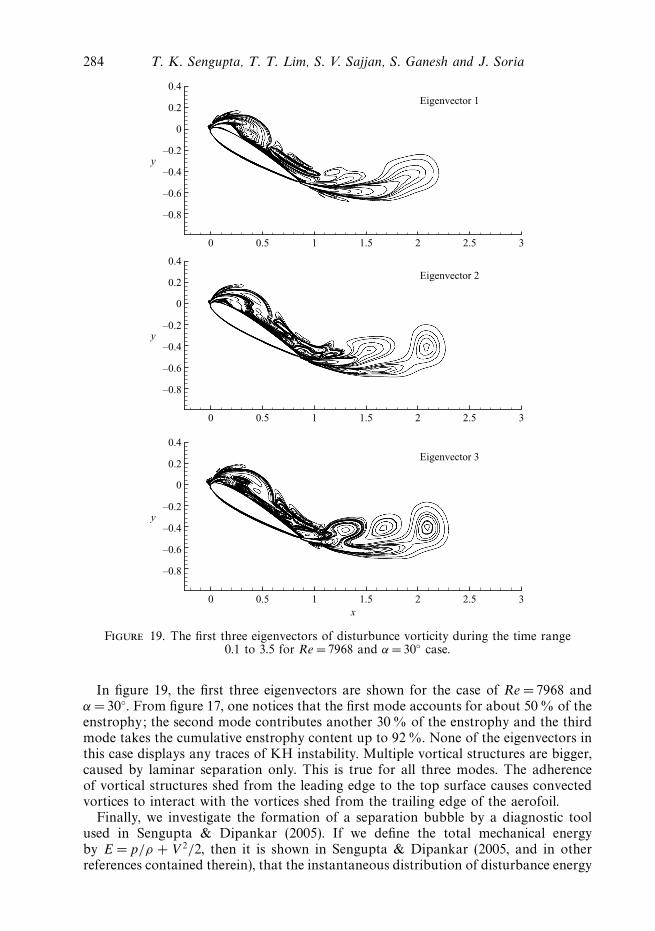
Figure 19. The first three eigenvectors of disturbunce vorticity during the time range0.1 to 3.5 for Re = 7968 and α = 30◦ case.

In figure 19, the first three eigenvectors are shown for the case of Re = 7968 andα = 30◦. From figure 17, one notices that the first mode accounts for about 50 % of theenstrophy; the second mode contributes another 30 % of the enstrophy and the thirdmode takes the cumulative enstrophy content up to 92 %. None of the eigenvectors inthis case displays any traces of KH instability. Multiple vortical structures are bigger,caused by laminar separation only. This is true for all three modes. The adherenceof vortical structures shed from the leading edge to the top surface causes convectedvortices to interact with the vortices shed from the trailing edge of the aerofoil.

Finally, we investigate the formation of a separation bubble by a diagnostic toolused in Sengupta & Dipankar (2005). If we define the total mechanical energyby E = p/ρ + V 2/2, then it is shown in Sengupta & Dipankar (2005, and in otherreferences contained therein), that the instantaneous distribution of disturbance energy


t = 2.00

t = 2.50

t = 3.00

t = 3.50

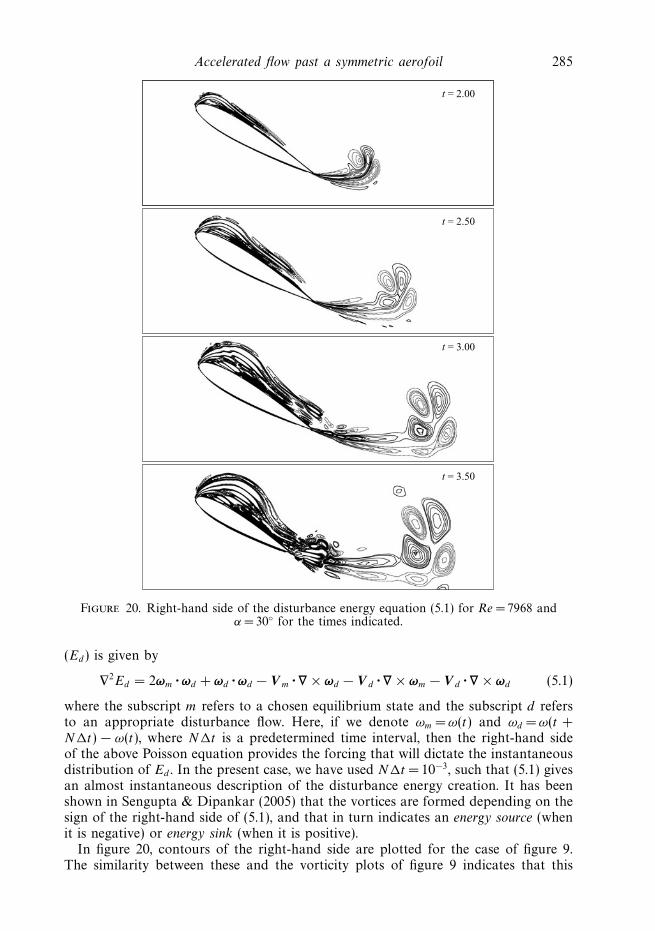
Figure 20. Right-hand side of the disturbance energy equation (5.1) for Re = 7968 andα = 30◦ for the times indicated.

(Ed) is given by

∇2Ed = 2ωm · ωd + ωd · ωd − V m · ∇ × ωd − V d · ∇ × ωm − V d · ∇ × ωd (5.1)

where the subscript m refers to a chosen equilibrium state and the subscript d refersto an appropriate disturbance flow. Here, if we denote ωm =ω(t) and ωd = ω(t +N�t) − ω(t), where N�t is a predetermined time interval, then the right-hand sideof the above Poisson equation provides the forcing that will dictate the instantaneousdistribution of Ed . In the present case, we have used N�t = 10−3, such that (5.1) givesan almost instantaneous description of the disturbance energy creation. It has beenshown in Sengupta & Dipankar (2005) that the vortices are formed depending on thesign of the right-hand side of (5.1), and that in turn indicates an energy source (whenit is negative) or energy sink (when it is positive).

In figure 20, contours of the right-hand side are plotted for the case of figure 9.The similarity between these and the vorticity plots of figure 9 indicates that this


type of vortex-dominated flow is dictated by the mechanism of disturbance energycreation given by (5.1) that is adequate when using the solution of two-dimensionalNavier–Stokes equation.

6. Summary and concluding remarksIncompressible accelerated flow past an aerofoil is studied here experimentally and

computationally at low Reynolds numbers and high angles of attack. Different typesof acceleration are considered, for which the major effects seen are related to unsteadyflow separation and their instabilities.

Specifically, a constant acceleration case and another case where the free-streamspeed reaches its final value via a non-uniform acceleration following a tangenthyperbolic variation are studied. For both cases, limited experimental results areavailable and additional experiments were conducted for NACA 0015 aerofoilexperiencing uniform acceleration for Re = 7968 and an angle of attack of α =30◦.The experiments have been performed in a piston-driven closed-circuit water tunnel.Experimentally obtained velocity and vorticity fields through PIV measurements havebeen presented in figures 4 and 5 for three different levels of accelerations in thepiston-driven water tunnel. It is noted from these results that the unsteady separationleading to bubble formation depends more on the duration of applied accelerationthan on the severity of the acceleration.

Computational results have been presented for different cases using an accuratemethod to solve time-dependent two-dimensional Navier–Stokes equations in streamfunction–vorticity formulation. This methodology has been well-tested on manyproblems of unsteady flows undergoing transition. The case of uniform accelerationthat displayed maximum unsteady separation in the experiments performed have beenstudied computationally and the results compared in figures 8 and 9. We have alsomeasured the flow velocity in the tunnel and noted some variations with the pistonvelocity as shown in figures 7(b) and 7(c). The reason for the difference is traced tothe fluid loading in the tunnel causing a small deformation of the square section.Despite the small variations between these two cases, we note only small differencesand found that the simulations performed with actual measured velocity match betterwith the experimental data. Since the measured velocity was low-pass filtered, thecomparison should improve further, if the higher frequency components of the actualvelocity are also included.

To study the effects of different types of accelerations, experimental results ofMorikawa & Gronig (1995) were simulated for Re = 35 000 and α =30◦, whenthe free-stream speed varies according to equation (1.1). Comparison between theexperimental results and computations shows very good agreement (see figure 10)when the computations are performed with the actual time variation of the freestream. Our computed results show even better agreement with the experiment thanthat provided in Morikawa & Gronig (1995) by a finite volume formulation. Thisestablishes the superiority of the formulation and methods employed in the presentstudy.

Effects of higher angles of attack have been investigated by computing some casesreported in Freymuth (1985) for Re =5200, with the flow experiencing accelerationlevels eighty times higher than in our experiments. The cases computed here are forα = 60◦ and 90◦ and the comparisons are shown in figures 12, 13 and 15. Displayedresults in figures 12 to 16 show the central importance of Kelvin–Helmholtz (KH)type instability of the separated shear layer at these high angles of attack. It is


also noted that the agreement between the experiments and the computations isparticularly good for the top part of the flow that shows shedding of clockwisevortices that undergo KH instability to create smaller vortices. The agreement is lesssatisfactory for the weaker bubble created at the trailing edge. Calculations revealbackscatter or merger of smaller vortices near the trailing edge, a well-known featureof two-dimensional simulations. This leads us to believe that the flow is affected moreby three-dimensionality near the trailing edge than the leading edge. This can explaincomputational observations.

The lack of small-scale vortices formed by KH instability for lower angles of attackis also supported by the POD results shown in figures 17 to 19, for the cases whosevorticity contours are shown in figures 9 and 12. It is noted that for the lower angleof attack (α =30◦), there is no evidence of KH instability, and the bubble formednear the leading edge slowly convects down the top surface and interact with vorticesformed at the trailing edge. The first eigenvector accounts for nearly 50 % of thetotal enstrophy and overall only five modes are necessary to represent 99 % of totalenstrophy. For the α = 60◦ case, first mode accounts for 70 % of total enstrophyand 11 modes are needed to describe 99 % of total enstrophy. It is noted that thevortical structures in the near wake are elongated in the streamwise direction for thelow angle of attack case, while for the higher angle of attack, the structures occupythe full base region. Finally, vortex creation by the disturbance energy description ofSengupta & Dipankar (2005) is analysed for a case tested and computed here. Closecorrespondence of vortex location with the location of the major disturbance sourcesand sinks establishes the utility of (5.1) as a diagnostic tool to predict flow separation.

REFERENCES

Badr, H. M., Dennis, S. C. R. & Kocabiyik, S. 1996 Symmetrical flow past an accelerated circularcylinder. J. Fluid Mech. 308, 97–110.

Brachet, M., Meneguzzi, M., Politano, H. & Sulem, P. 1988 The dynamics of freely decayingtwo-dimensional turbulence. J. Fluid Mech. 194, 333–349.

Brendel, M. & Mueller, T. J. 1988 Boundary-layer measurements on an airfoil at low Reynoldsnumbers. J. Aircraft 25, 612–617.

Carr, L. W. & Chandrasekhara, M. S. 1996 Compressibility effects on dynamic stall. Prog. Aero.Sci. 32, 523–573.

Choudhuri, P. G. & Knight, D. D. 1996 Effects of compressibility, pitch rate, and Reynolds numberon unsteady incipient leading-edge boundary layer separation over a pitching aerofoil. J. FluidMech. 308, 195–217.

Collins, W. M. & Dennis, S. C. R. 1974 Symmetrical flow past a uniformly accelerated circularcylinder. J. Fluid Mech. 65, 461–480.

Currier, J. F. & Fung, K. Y. 1992 Analysis of the onset of dynamic stall. AIAA J. 30, 2469–2477.

Freymuth, P. 1985 The vortex patterns of dynamic separation: a parametric and comparative study.Prog. Aero. Sci. 22, 161–208.

Gendrich, S. C., Koochesfahani, M. M. & Visbal, M. R. 1995 Effects of initial acceleration onthe flow field development around rapidly pitching airfoils. Trans. ASME: J. Fluids Engng117, 45–49.

Huang, R. F. & Lin, C. L. 1995 Vortex shedding and shear-layer instability of wing at low-Reynoldsnumbers. AIAA J. 33, 1398–1403.

Koochesfahani, M. M. & Smiljanovski, V. 1993 Initial acceleration effects on flow evolutionaround airfoils pitching to high angles of attack. AIAA J. 31 1529–1531.

Lesieur, M. & Metais, O. 1996 New trends in large-eddy simulations of turbulence. Annu. Rev.Fluid Mech. 28, 45–82.

Lin, J. C. M. & Pauley, L. L. 1996 Low-Reynolds-number separation on an airfoil. AIAA J. 34,1570–1577.


Lugt, H. J. & Haussling, H. J. 1978 The acceleration of thin cylindrical bodies in a viscous fluid.J. Appl. Mech. 45, 1–6.

Mathaeus, W. H., Stribling, W. T., Martinez, D., Oughton, S. & Montgomery, D. 1991 Selectivedecay and coherent vortices in two-dimensional incompressible turbulence. Phys. Rev. Lett.66, 2731–2734.

McCroskey, W. J. 1982 Unsteady airfoils. Annu. Rev. Fluid Mech. 24, 285–311.

Mehta, U. B. & Lavan, Z. 1975 Starting vortex, separation bubbles and stall: a numerical study oflaminar unsteady flow around an airfoil. J. Fluid Mech. 67, 227–256.

Morikawa, K. & Gronig, H. 1995 Formation and structure of vortex systems around a translatingand oscillating airfoil. Z. Flugwiss. Weltraumforsch 19, 391–396.

Nair, M. T. 1998 Accurate numerical simulation of two-dimensional unsteady incompressible flows.PhD Thesis, Dept. Aero. Engng, Indian Institute of Technology Kanpur, India.

Nair, M. T. & Sengupta, T. K. 1997a Unsteady flow past elliptic cylinders. J. Fluids Struct. 11,555–595.

Nair, M. T & Sengupta, T. K. 1997b Accelerated incompressible flow past aerofoils. Proc. 7thAsian Congress of Fluid Mechanics Madras, India, Dec. 1997.

Nair, M. T. & Sengupta, T. K. 1998 Orthogonal grid generation for Navier-Stokes computations.Intl J. Numer. Meth. Fluids 28, 215–224.

Nair, M. T., Sengupta, T. K. & Chauhan, U. S. 1998 Flow past rotating cylinders at high Reynoldsnumbers using higher order upwind scheme. Computers Fluids 27(1), 47–70.

Ohmi, K., Coutanceau, M., Loc, T. P. & Dulieu, A. 1991 Further experiments on vortex formationaround an oscillating and translating airfoil at large incidences. J. Fluid Mech. 225, 607–630.

Perry, A. E., Chong, M. S. & Lim, T. T. 1982 The vortex shedding process behind two-dimensionalbluff bodies. J. Fluid Mech. 116, 77–90.

Ramiz, M. A. & Acharya, M. 1992 Detection of flow state in an unsteady separating flow. AIAAJ. 30, 117–123.

Rayleigh, Lord 1911 On the motion of solid bodies through viscous liquids. Phil. Mag. (6) 21,697–711.

Sarpkaya, T. 1991 Nonimpulsively started steady flow about a circular cylinder. AIAA J. 29,1283–1289.

Schlichting, H. 1979 Boundary Layer Theory, VII edn. McGraw Hill.

Sengupta, T. K. 2004 Fundamentals of Computational Fluid Dynamics. Universities Press, Hyderabad,India.

Sengupta, T. K. & Dipankar, A. 2005 Subcritical instability on the attachment-line of an infiniteswept wing. J. Fluid Mech. 529, 147–171.

Sengupta, T. K., Ganeriwal, G. & De, S. 2003 Analysis of central and upwind compact schemes.J. Comput. Phys. 192, 677–694.

Sengupta, T. K., Vikas, V. & Johri, A. 2006 An improved method for calculating flow past flappingand hovering airfoils. Theor. Comput. Fluid Dyn. 19, 417–440.

Sirovich, L. 1987 Turbulence and the dynamics of coherent structures. Parts 1-3: Coherentstructures. Q. Appl. Maths 45, 561–584.

Soria, J., New, T. H., Lim, T. T. & Parker, K. 2003 Multigrid CCDPIV measurements of acceleratedflow past an airfoil at an angle of attack of 30◦. Expl Therm. Fluid Sci. 27, 667–676.

Stokes, G. G. 1851 On the effect of the internal friction of fluids on the motion of pendulums.Trans. Camb. Phil. Soc. 9, 8–106.

Stuart, J. T. 1963 Unsteady boundary layers. In Laminar Boundary Layers (ed. L. Rosenhead).Clarendon Press.

Sugavanam, A. & Wu, J. C. 1982 Numerical study of separated turbulent flow over airfoils. AIAAJ. 20, 464–470.

Zaman, K. B. M. Q., McKinzie, D. J. & Rumsey, C. L. 1989 A natural low-frequency oscillationof the flow over an airfoil near stalling conditions. J. Fluid Mech. 202, 403–442.

Accelerated flow past a symmetric aerofoil: experiments and computations

Documents

Transcript of Accelerated flow past a symmetric aerofoil: experiments and computations