
Ability of a global three-dimensional model to locate regional events
68
-
Upload
independent -
Category
Documents
-
view
1 -
download
0
Transcript of Ability of a global three-dimensional model to locate regional events

JOURNAL OF GEOPHYSICAL RESEARCH, VOL. , NO. , PAGES 1{42,
The ability of a global 3-D model to locate
regional events
M.H. Ritzwoller, N.M. Shapiro, A.L. Levshin, E.A. Bergman, E.R. Engdahl
Center for Imaging the Earth's Interior, Department of Physics, University
of Colorado at Boulder, Boulder, Colorado, USA
Resubmitted after review to J. Geophys. Res., March 31, 2003.
M.H. Ritzwoller, Department of Physics, University of Colorado at Boulder, Boulder, CO
80309-0390, USA. ([email protected])
N.M. Shapiro, Department of Physics, University of Colorado at Boulder, Boulder, CO 80309-
0390, USA. ([email protected])
A.L. Levshin, Department of Physics, University of Colorado at Boulder, Boulder, CO 80309-
0390, USA. ([email protected])
E.A. Bergman, Department of Physics, University of Colorado at Boulder, Boulder, CO 80309-
0390, USA. ([email protected])
E.R. Engdahl, Department of Physics, University of Colorado at Boulder, Boulder, CO 80309-
0390, USA. ([email protected])
D R A F T April 18, 2003, 2:16pm D R A F T

2 RITZWOLLER ET AL.: GLOBAL MODEL AND REGIONAL EVENTS
Abstract. We assess the ability of a global 3-D seismic model of the crust
and upper mantle (CUB2.0) to locate seismic events using regional travel time
data alone (epicentral distances < 20�). Assessments are based on a \Ground
Truth" (GT) data base comprising nearly 1000 uncommonly well located events
which occur in 23 event clusters across Eurasia and North Africa, groomed
P and Pn arrival time data observed at regional distances from individual
events, and about 1000 empirical phase path anomalies produced from event
clusters. Evidence is presented that supports the conversion of the shear ve-
locities (vs) in CUB2.0 to compressional velocities (vp) in the upper man-
tle using the thermoelastic properties of an assumed mantle composition rather
than traditional empirical scaling relationships. Two principal results are pre-
sented. First, this 3-D vp model �ts the empirical P and Pn phase path anoma-
lies very well in both pattern and absolute level. Second, location assessments
demonstrate that intrinsic regional location accuracy is �5 km using the 3-
D vp model and �10 km using the 1-D model AK135. These �ndings high-
light the importance of GT data bases in assessing regional travel time mod-
els and establish that a global 3-D vs model, together with vp inferred from
it, provide a solid basis on which to build improvements in regional location
capabilities.
D R A F T April 18, 2003, 2:16pm D R A F T
RITZWOLLER ET AL.: GLOBAL MODEL AND REGIONAL EVENTS 3
1. Introduction
The seismic location inverse problem has a history dating back almost a century, at least
to Geiger [1912]. There has been a recent resurgence of interest in improving abilities to
estimate reliable seismic locations for both earthquakes and explosions [e.g., Thurber &
Rabinowitz, 2000]. One reason for this resurgence is the desire to apply advances in seis-
mological models and practice to improve event locations in global catalogs produced, for
example, by the International Seismological Centre (ISC), the U.S. National Earthquake
Information Service (NEIS), or the International Data Center (IDC). Another reason is
that the Comprehensive Nuclear Test-Ban Treaty (CTBT), irrespective of its current sta-
tus, has motivated greater emphasis on locating small natural or human-produced seismic
events. The CTBT speci�es a location uncertainty of 1000 km2 or less for events with
magnitudes greater than or equal to 4.0 [e.g., Ringdal & Kennett, 2001]. In addition,
there has been growing recognition of the importance of high quality locations in seismic
tomography and fault zone characterization.
E�orts to improve the location of seismic events have fallen into two broad categories:
advances in seismic travel time models to improve absolute locations and innovations in
location methods, in particular using multiple event location methods to improve relative
location capabilities [e.g., Poupinet et al., 1984; Fr�emont & Malone, 1987; Pavlis, 1992;Got
et al., 1994; Waldhauser & Ellsworth, 2000]. These categories are not mutually exclusive
and each possesses characteristic strengths and limitations. The emphasis of this paper
will be on testing a speci�c type of travel time model in which regional seismic phases
are computed from a global 3-D seismic model. The key words here are \regional" and
\global 3-D seismic model" which we describe further here.
D R A F T April 18, 2003, 2:16pm D R A F T
4 RITZWOLLER ET AL.: GLOBAL MODEL AND REGIONAL EVENTS
The phrase \regional" refers to epicentral distances less than about 20�, in contrast with
teleseismic distances. At present, regional seismic phases remain relatively poorly studied
and modeled except in regions of the world that are heavily populated, seismically active,
and well instrumented (e.g., Western U.S., Japan, parts of Europe, part of China, etc.).
Regional data, therefore, are typically weighted down strongly in location procedures
that mix regional and teleseismic phases. In particular, the need for consistency in global
catalogs has inhibited the adoption of modern seismic models in the major global seismic
catalogs. For example, the ISC and the NEIS continue to use the Je�reys-Bullen travel-
time tables [Je�reys & Bullen, 1940] and the IDC uses travel times from the 1-D model
IASP91 [Kennett & Engdahl, 1991], neither of which is designed to �t regional travel
times nor identify regional phases. Substantial improvements in global seismicity catalogs
would derive through better use of regional data, which would be made possible by better
travel time models. In addition, the concentration of monitoring e�orts stimulated by
the CTBT has focused attention on small seismic events that may be clandestine nuclear
explosions. Small events are recorded primarily at regional distances, perhaps with a few
reported teleseismic phases. The on-site inspection provisions of the CTBT also require
the locations of these small events to be of high quality. The focus of research e�orts
motivated by the technical requirements of the CTBT, therefore, is on regional locations
with a sparse network of recording stations.
Our concentration will be on travel time models derived from a \global 3-D seismic
model", in contrast with travel time models that derive from local models or directly from
observations of regionally propagating seismic phases such as Pn. Although high quality
regional travel time observations from well located events are available in some regions
D R A F T April 18, 2003, 2:16pm D R A F T
RITZWOLLER ET AL.: GLOBAL MODEL AND REGIONAL EVENTS 5
of the world (e.g., China, parts of Europe, Japan, Western U.S., parts of Russia and the
former Soviet Republics, etc.), this information is sparse within a world-wide context and
may exist for only certain phases, most commonly Pn. The advantage of using a global
3-D seismic model to predict regional travel times is that the model exists everywhere and
can be used to predict the travel times of all seismic phases, although probably not with
equal accuracy. If they are su�ciently accurate, the travel times computed using a global
3-D model would provide the foundation on which to build future improvements, such as
assimilating observations of regional phases and regional travel time models where they
exist. The assimilation of regional empirical information, however, requires international
cooperation as well as a strong will to achieve. In lieu of this e�ort, travel times from a
global 3-D model across much of the earth's surface may be the best feasible alternative
now and in the near future. They also provide a benchmark to improve upon in developing
future capabilities, a role similar to that played by 1-D travel time models now.
To date, most published attempts to improve body wave travel time models have been
devoted to improving teleseismic location capabilities by concentrating on the application
of current-generation 1-D and 3-D mantle models. For example, Engdahl et al. [1998]
showed that global improvements in teleseismic locations are possible by applying new
methods using the 1-D model AK135 [Kennett et al., 1995]. Several researchers have in-
vestigated how the use of 3-D tomographic models of the whole mantle a�ect hypocenter
determinations based on teleseismic travel time data [e.g., Smith & Ekstr�om, 1996; Antolik
et al., 2001; Chen & Willemann, 2001]. These studies established that teleseismic misloca-
tions are reduced relative to 1-D model locations (e.g., Je�reys-Bullen travel-time tables,
PREM [Dziewonski & Anderson, 1981], IASP91 [Kennett & Engdahl, 1991]) when recent
D R A F T April 18, 2003, 2:16pm D R A F T
6 RITZWOLLER ET AL.: GLOBAL MODEL AND REGIONAL EVENTS
generation 3-D mantle models based on either global [e.g., Su et al., 1994; Su & Dziewon-
ski, 1997] or local basis functions [e.g., van der Hilst et al., 1997; Bijwaard et al., 1998;
Boschi & Dziewonski, 1999] are applied. E�orts to predict teleseismic travel times with
empirical teleseismic heterogeneity corrections have been more rare, but show promise
[e.g., Piromallo & Morelli, 2001].
At regional distances, travel time predictions depend on the ability to model the crust
and upper mantle. Regional travel time predictions are less accurate than teleseismic
predictions because heterogeneity is much stronger and because data that constrain the
crust and upper mantle are more limited in distribution and somewhat more di�cult to
interpret unambiguously. For example, regional triplication crossover distances are highly
variable which makes it di�cult to identify phases correctly. This is true both for Pn
triplications, as well as for distinguishing Pn from P arrivals. For these reasons, model-
based approaches to predicting regional travel times [e.g., Firbas, 2000] have played a
subordinate role to the development of purely empirical corrections [e.g.,Myers & Schultz,
2000] that may be combined with spatial interpolation schemes [e.g., Schultz et al., 1998].
The result is that the ability of 3-D models, particularly global models, to predict
regional travel times remains largely uninvestigated and, consequently, the applicability
of 3-D models to the problem of regional location is poorly understood. The purpose
of this paper is to help �ll in this gap in knowledge. Although our concentration is on
Eurasia, the general features of the results should also hold for shallow events on other
continents.
We are able to perform the study of the utility of a global 3-D model to improve regional
locations because of two recent advances. First, we have developed a global 3-D model of
D R A F T April 18, 2003, 2:16pm D R A F T

RITZWOLLER ET AL.: GLOBAL MODEL AND REGIONAL EVENTS 7
the crust and uppermost mantle that is designed speci�cally to be used to predict regional
travel times. To predict reliable regional travel times it is, �rst, desirable that the model
exists throughout the region of study. It is also necessary for attention to be paid to
the crustal part of the model and, because regional travel times are controlled largely
by the turning point of the ray, to the vertical gradient of the model. For regional travel
times, the vertical resolution is probably more important than the lateral resolution of the
model. To satisfy these criteria we use a 3-D vs model derived from surface wave dispersion
which we convert to vp by applying information about the thermoelastic properties of an
assumed mantle composition. The use of a vs model to predict regional vp travel times is
not ideal, but is the consequence of the existence of much better information about upper
mantle vs than vp structure.
The second advance is the development of a unique data base of nearly 1000 \Ground
Truth" (GT) locations in 23 event clusters across much of Eurasia. These locations,
together with the groomed arrival time data set and the empirical phase path anomalies
that emerge for each cluster, provide information needed to determine the capability of
any travel time model or set of empirical travel time correction surfaces to predict regional
travel times and locate seismic events using regional travel time data alone.
We restrict the study to the use of P and Pn travel times for stations within 20� of the
source locations. While optimal regional locations would include crustal phases as well as
later P phases and S phases, the consideration of these phases is not necessary to test the
performance of the 3-D model and, in fact, unnecessarily complicates the interpretation
of the location exercise.
D R A F T April 18, 2003, 2:16pm D R A F T
8 RITZWOLLER ET AL.: GLOBAL MODEL AND REGIONAL EVENTS
In section 2, we discuss the procedure used to construct the data base of GT locations,
the groomed arrival time data set, and the empirical phase path anomalies for each event
cluster. The 3-D model construction and the ray-tracing procedure are discussed in section
4. The �rst test of the 3-D model is its ability to predict regional travel times. We discuss
the �t to the empirical phase path anomalies in section 5. The second test of the 3-D
model is the ability to locate the GT events using regional data alone. The grid-search
location procedure is described in section 6 and the location tests are presented in section
7.
2. Validating Data Set
2.1. Motivation
The assessment of a seismic velocity model requires a validating data set that is inde-
pendent of the data used to derive the model. For this study, we have assembled a data
set of seismic events whose locations and origin times are known with greater than usual
accuracy, either because they have been located with a local seismic network or because
they were anthropogenic explosions. These so-called \Ground Truth" (GT) events are
used to obtain reliable empirical estimates of source-station path anomalies (relative to a
1-D reference model) that can be compared with predictions from seismic models. The
known locations of the GT events can also be compared to locations obtained from seismic
models.
In this section, we discuss the development of the validating data set by multiple event
relocation of clustered earthquake and explosion sequences in Eurasia and northern Africa.
Primarily, we use phase arrival time data reported to the ISC and to the NEIS, but for
some clusters we have obtained additional data (usually at regional distances) from other
D R A F T April 18, 2003, 2:16pm D R A F T
RITZWOLLER ET AL.: GLOBAL MODEL AND REGIONAL EVENTS 9
sources. The arrival time data are �rst \groomed" on an event by event basis, using a
procedure described by Engdahl et al. [1998] in the development of the EHB catalog. A
multiple event location method is then used to re�ne the locations and identify outliers
in the arrival time data. The resulting catalog of GT events, the groomed travel time
data base, and the empirical phase path anomalies create a data base that can be used in
experiments to assess 3-D models and to address systematic errors in event location.
The Ground Truth events occur in the clusters shown in Figure 1 and are listed in Table
1.
2.2. The GT Location Data Base
We seek clusters of earthquakes where at least one of the events has been very well
located by a local seismic network or a temporary deployment of instruments, commonly
in after-shock studies. We have used events from 1964-2001 in this study. The clusters
typically are 50-100 km across and comprise up to about 100 events of magnitude 3.5 or
greater that are well recorded at regional and teleseismic distances.
The multiple event location method used in this study is based on the Hypocentroidal
Decomposition (HDC) method [Jordan & Sverdrup, 1981], which is schematically illus-
trated in Figure 2. The EHB single-event locations are used as the starting locations
for the HDC analysis, which converges in several iterations. We perform HDC analysis
many times on each cluster, however, in the process of identifying outliers and estimating
empirical reading errors.
The depths for all events were �xed in the HDC analysis. We �xed depths at the local
network determination of focal depth for those events for which we have that information,
and at an optimum depth (usually an average of the local network depths) for all remaining
D R A F T April 18, 2003, 2:16pm D R A F T
10 RITZWOLLER ET AL.: GLOBAL MODEL AND REGIONAL EVENTS
events in the cluster. To ensure that no gross errors in the assumed focal depths are made,
we also examined reported depth phases at teleseismic distances [Engdahl et al., 1998].
We refer to the resulting set of 989 locations listed in Table 1 as the GT locations.
The accuracy of the GT locations and the shift in the origin time (\cluster time baseline
shift") are discussed further below.
The reference event source parameters, which form the heart of the GT data base, were
compiled from many sources, but were based exclusively on work done by the original
investigators in each source region. We attempt to validate the claimed accuracy and
assign a GT level of accuracy by analyzing the local network data and through tests of
consistency with the HDC results. We discovered that many proposed reference events are
in fact seriously mislocated. The consistency between the relative locations as determined
by HDC analysis of global arrival time data and the relative locations derived from the
reference event data is one of the criteria we use to validate candidate reference events.
Shifts in epicenter and origin time to match the reference event locations are typically in
the range of 5-15 km and �2 seconds, respectively.
We follow Bondar et al. [2003] and represent location con�dence bounds using the
Ground Truth GTXC% classi�cation, where the \X" su�x designates location accuracy
in km and C% is the percent con�dence. For simplicity here, we report only 95% con�dence
bounds, so that, for example, a GT5 classi�cation represents 95% con�dence in location
accuracy of 5 km or better.
We use the \GT-level" classi�cations in two senses. First, is the sense of the accuracy
level of individual reference events, as discussed above. Second, we use the same concept
to describe the level of accuracy of entire clusters after shifting to best match the reference
D R A F T April 18, 2003, 2:16pm D R A F T

RITZWOLLER ET AL.: GLOBAL MODEL AND REGIONAL EVENTS 11
locations. The GT-level assigned to a cluster is more subjective, related to the GT-level
of individual reference events, the number of reference events, the degree of consistency
between the relative locations as expressed by the HDC analysis and reference data, and
other factors. For example, the Aqaba cluster is calibrated by a single reference event,
which quali�es as GT5, but we assign the cluster a GT10 level of accuracy because there
is only a single reference event and because the event occurred in a region of very strong
lateral heterogeneity, the transition from continental to oceanic lithosphere.
We shift the hypocentroid in space and time to achieve the best �t for absolute locations
and origin times between the HDC-derived locations and the reference event locations,
as illustrated in Figure 2d. The \cluster time baseline shift" is the average di�erence
between the reference event origin times and the origin times obtained by HDC analysis
for those same events (Table 1). This correction is added to the HDC-derived origin times
to produce a best estimate of absolute origin times. Positive corrections (i.e., shorter
travel times) indicate faster velocities relative to AK135. The cluster time baseline shift
arises in part from di�erences between the 1-D model travel time used in the HDC analysis
and the true travel times, but may also re ect bias in the reference event origin times.
Myers & Schultz [2001] have shown that origin times estimated from local network data
can be biased by several seconds if the local velocity model is not well-calibrated, even
though the hypocenters may be estimated with high accuracy. The cluster time baseline
shifts assist in phase identi�cation and are also used to compare results between clusters
and are included in estimates of empirical phase path anomalies relative to AK135, as
discussed below.
D R A F T April 18, 2003, 2:16pm D R A F T
12 RITZWOLLER ET AL.: GLOBAL MODEL AND REGIONAL EVENTS
This method has resulted in a data base of 23 event clusters, including 6 explosion
clusters with source locations generally known to better than 2 km, and 17 earthquake
clusters, 11 of whose locations are believed to be accurate to within 5 km and the remainder
to within 10 km. There are 989 events that compose these 23 clusters of which 753 are
GT5 or better. The locations of the clusters studied are plotted in Figure 1. Relevant
parameters for all clusters are listed in Table 1. The location and depth given are for the
shifted hypocentroid, representing the best �t to reference event locations.
2.3. The Groomed Arrival Time Data Set
Multiple event location e�ciently rejects outliers which results in a data set of
\groomed" arrival times for each of the events in the GT data base. The number of
these data is listed in Table 2 and Figure 3 shows a plot of the Pn and P residuals for all
groomed arrival times included in this data base, adjusted by the cluster time baseline
shift. Estimates of the residual median and spread show considerable variation over the
regional distance range. In particular, residuals for Pn arrivals between about 9 and 17
degrees, corresponding to ray paths bottoming in the lithosphere well below the crust and
perhaps encountering low velocity zones, are more spread, with a maximum spread at dis-
tances of 12-13 degrees. A contributing factor to this spread at larger regional distances
is the di�culty of phase identi�cation; e.g., distinguishing between various Pn branches
or between Pn and P in regions where the crossover distance between the �rst-arriving
branches of these phases is poorly known.
D R A F T April 18, 2003, 2:16pm D R A F T
RITZWOLLER ET AL.: GLOBAL MODEL AND REGIONAL EVENTS 13
2.4. The Empirical Phase Path Anomalies
The basic premise of all multiple event location methods is that path anomalies from
each station to all observed events in a given cluster are correlated. Thus, multiple
event location analysis produces robust estimates of source-station path anomalies that
are far more di�cult to extract from single event location catalogs. The set of groomed
residuals for regional P and Pn, relative to shifted hypocenters derived by HDC analysis
and adjusted for cluster time baseline shifts, are used to calculate source-station phase
path anomalies. These anomalies are estimated relative to the 1-D reference model AK135.
Medians and spreads for all groomed residuals for each cluster are calculated for the phases
of interest (primarily P and Pn, here) at each of the reporting stations for that cluster.
The resulting source-station \empirical phase path anomalies" (the median) are accepted
with a minimum requirement of �ve observations and a spread of less than 1.40 sec for
P�type phases. (\Spread" is a robust analog to the standard deviation.)
At regional distances there are 836 Pn and 178 P path anomalies, respectively. Results
are plotted in Figure 4. These empirical estimates range from about -7.5 sec to +5.0 sec,
with the largest anomalies occurring at distances from 11 to 18 degrees (similar to Figure
3). In this distance range, Pn typically has a triplication and P has a back branch (Figure
4b) making phase identi�cation di�cult.
3. Evaluation Metric
In section 2 we described three data sets that are useful for assessing 3-D seismic models.
First, there is the set of 989 GT locations that are available to test location capabilities.
In fact, only 753 of these events are identi�ed as GT5 or better, and it is these events
that will be most useful in this study. Second, there is the groomed travel time data,
D R A F T April 18, 2003, 2:16pm D R A F T
14 RITZWOLLER ET AL.: GLOBAL MODEL AND REGIONAL EVENTS
particularly regional P and Pn, from the ISC and NEIS bulletins as well as some data
from regional networks, that formed the basis for the HDC analyses. These data are used
to relocate the GT events in section 7 below. Finally, there are the empirical phase path
anomalies that in section 5 are compared with the travel times predicted from several
models (both 1-D and 3-D).
Studies aimed at evaluating the location capabilities of certain models or location tech-
niques commonly concentrate exclusively on the accuracy of the locations relative to some
benchmark. Although this is also an important part of the present study, we argue that
the ability to model regional travel time data is a better measure of the quality of 3-D
models and is, in fact, a more robust predictor of regional location capabilities. This
is because evaluations based on location alone are complicated by a variety of factors
that inhibit clear assessment; e.g., variations in network geometry from one region to
another, di�erent mixes of regional phases, di�erential quality of reported travel times,
and so forth. The carefully constructed empirical phase path anomaly data set gives us
con�dence that assessments of the �t to regional travel time data provide meaningful,
relatively unambiguous information about the quality of the models. The groomed travel
time data set alone is probably too noisy to be used for this purpose.
4. 3D Model and Travel Time Computation
4.1. Model Construction
The 3-D model is based on broad-band surface wave group and phase speed measure-
ments. The group velocities were measured using the frequency - time method described
by Ritzwoller & Levshin [1998], which involves analyst interaction to choose the frequency
band of measurement and to guide the extraction of the fundamental mode from noise,
D R A F T April 18, 2003, 2:16pm D R A F T

RITZWOLLER ET AL.: GLOBAL MODEL AND REGIONAL EVENTS 15
scattered and multipathed signals, overtones, and fundamental modes of di�erent wave
types. We use group speed measurements from 16 s to 200 s period for Rayleigh waves
and from 16 s to 150 s period for Love waves. The phase speed measurements were per-
formed at Harvard University [Ekstr�om et al., 1997] and Utrecht University [Trampert and
Woodhouse, 1995] separately and we merged these data sets. The phase speed measure-
ments extend from 40 s to 150 s for both Rayleigh and Love waves. We use measurements
only from earthquakes shallower than 50 km to reduce the size of the source group time
shifts, which we do not attempt to correct [Levshin et al., 1999]. All measurements are
subjected to the quality control procedures described by Ritzwoller & Levshin [1998], but
the number of group speed measurements has multiplied several times since that study.
The construction of the group and phase speed maps uses the tomographic method
described by Barmin et al. [2001], which is based on geometrical ray-theory with intuitive
Gaussian smoothing constraints to simulate surface wave sensitivities. We refer to this
method as Gaussian tomography. In fact we apply an update of this method [Ritzwoller
et al., 2002a], referred to as di�raction tomography, which uses a simpli�ed version of
the scattering sensitivity kernels that emerge from the Born or Rytov approximations.
Di�raction tomography accounts for path-length-dependent sensitivity, wave-front healing
and associated di�raction e�ects, and provides a more accurate assessment of spatially
variable resolution than traditional tomographic methods. The resolution procedure is
described by Barmin et al. [2001]. We produce a resolution surface at every nodal point
on the globe, �t a cone to the surface in the neighborhood of each node, and de�ne
resolution as the half-width of the base of the cone (or identically, the full-width at half-
max). Surface wave resolution estimates averaged over the region of study are presented
D R A F T April 18, 2003, 2:16pm D R A F T
16 RITZWOLLER ET AL.: GLOBAL MODEL AND REGIONAL EVENTS
in Figure 5. Surface wave Fresnel zones widen appreciably at long periods and narrow only
near sources and receivers, so resolution is best at short periods and in areas with sources
or receivers. The dispersion maps are produced on a 2� � 2� grid world-wide. Di�raction
tomography a�ects the amplitude and geometry of the dispersion features particularly
at long period, as described by Ritzwoller et al. [2002a]. Figures 6a and 6b show two
examples of surface wave dispersion maps across the region of study constructed with
di�raction tomography.
The shear velocity model is constructed using a Monte-Carlo method, which is described
in detail by Shapiro and Ritzwoller [2002]. The shear velocity model of Shapiro and
Ritzwoller [2002] was based on Gaussian tomography and is referred to here as CUB1.0.
The 3-D shear velocity model we use here is based on di�raction tomography and we
will refer to it as CUB2.0. These models only include vp in the crust. The vp part
of CUB2.0 in the mantle is derived by converting from vs using two di�erent methods,
We will distinguish between these two vp models by introducing su�ces to the names
(CUB2.0 TH, CUB2.0 EMP), as discussed below.
The inversion for a velocity pro�le is performed at each node on a 2� � 2� grid world-
wide, producing an ensemble of acceptable models down to a depth of 400 km. The
model is constrained by a variety of a priori information, including the initial crustal
model CRUST2.0 (G. Laske, personal communication) and the initial mantle model S20A
of Ekstr�om & Dziewonski [1998]. Perturbations are allowed within speci�ed tolerances
to both vs and vp in the crust, to vs in the mantle, and to Moho depth. The model is
radially anisotropic (vsh 6= vsv) from the Moho to a variable depth that averages about
200 km. The strength of radial anisotropy is constrained to decrease monotonically with
D R A F T April 18, 2003, 2:16pm D R A F T

RITZWOLLER ET AL.: GLOBAL MODEL AND REGIONAL EVENTS 17
depth and crustal speeds are constrained to increase monotonically with depth. Shapiro
and Ritzwoller [2002] fully describes the set of constraints and a priori information.
Figure 7 presents an example of the results of the Monte-Carlo inversion at a single
point. The center and half-width of the ensemble of acceptable models summarize the
model at each depth. The e�ective isotropic model, vs, is de�ned as the average of vsh
and vsv at each depth. Figures 7b-d show that model uncertainties are reduced and,
hence, vertical resolution is improved appreciably by simultaneously inverting the group
and phase speed curves. Using phase velocities alone produces large uncertainties in the
crust and, consequently, also in the upper mantle. Inverting group velocities alone yields
relatively small uncertainties in the crust and uppermost mantle due to the measurements
at periods shorter than 40 sec, but uncertainties deeper in the upper mantle are larger.
When phase and the group velocities are inverted simultaneously, however, uncertainties
are signi�cantly reduced at all depths. In particular, the simultaneous inversion of broad-
band group and phase speed data in the presence of a priori constraints on allowable
structures in the crust and upper mantle ameliorates the trade-o� between crustal and
upper mantle structures that plague inversions of surface waves in continental areas.
Figures 6c-d and 8 present horizontal and vertical slices of the vs model to demonstrate
the nature of the heterogeneities. It is noteworthy that the mantle features inferred from
di�raction tomography tend to have larger amplitudes and extend deeper than those from
Gaussian tomography. Based on the dispersion resolution information given in Figure 5,
we infer that average lateral resolution is between 400 and 500 km in the uppermost
mantle but degrades with depth. As length-scales in the model approach the estimated
resolution, however, the amplitude of heterogeneity tends to be underestimated.
D R A F T April 18, 2003, 2:16pm D R A F T
18 RITZWOLLER ET AL.: GLOBAL MODEL AND REGIONAL EVENTS
4.2. Conversion of vs to vp in the Mantle
To be able to predict Pn and P travel times, the 3-D vs model CUB2.0 must be converted
to a vp model. There are two general approaches to doing this. The �rst is to use \empirical
scaling relations" that convert vs anomalies into vp anomalies. The most successful of these
map shear-speed perturbations, �vs, relative to a reference S-model, vs0, to compressional-
velocity perturbations, �vp, relative to a reference P -model, vp0, where d ln vp=d ln vs is
then taken to be an empirically constrained constant that may be a function of depth,
but is usually depth invariant. The second approach is to use a \thermoelastic conversion"
based on laboratory measurements of thermoelastic properties of mantle minerals and on
models of the average mineralogical composition of the mantle. The vp model that results
from CUB2.0 vs by the thermoelastic conversion will be referred to here as CUB2.0 TH
and the vp model derived from the empirical scaling relation (d ln vs=d ln vp = 1:9) in which
the 1-D reference model is AK135 will be called CUB2.0 EMP. We convert only isotropic
vs to vp. In the radially anisotropic part of CUB2.0 we, therefore, use vs = (vsv + vsh)=2.
We prefer the thermoelastic conversion from vs to vp for two reasons. First, as we will
show below, the thermoelastic conversion appears to work somewhat better in that the
regional P and Pn empirical phase path anomalies are �t better by travel times predicted
by CUB2.0 TH than by CUB2.0 EMP. Second, the thermoelastic conversion leads natu-
rally to future improvement. It can be regionally tuned in a physically meaningful way
by modifying the mineralogical composition and temperatures within the anelastic model,
and it can be updated as better mineralogical data become available.
The thermoelastic conversion between vs and vp in the mantle is mediated by a conver-
sion to temperature. There have been numerous previous studies that have explored the
D R A F T April 18, 2003, 2:16pm D R A F T

RITZWOLLER ET AL.: GLOBAL MODEL AND REGIONAL EVENTS 19
relationship between the seismic velocities, temperature, and composition [e.g., Du�y &
Anderson, 1989; Graham et al., 1989; Furlong et al., 1995; Sobolev et al., 1996; Goes et al.,
2000; R�ohm et al., 2000; Trampert et al., 2001; van Wijk et al., 2001]. The method we
use here is based on that of Goes et al. [2000], and is described in detail by Shapiro and
Ritzwoller [2003]. The mantle is considered to be composed of four principal minerals.
The elastic moduli and density can be computed for each mineral independently as a
function of temperature, pressure, and iron content, extrapolating values of each quantity
at surface conditions to depth with zero iron content by using experimentally-determined
partial derivatives. For a speci�c mineralogical composition, the elastic moduli and den-
sity, and hence the seismic velocities, are computed using the Voigt-Reuss-Hill mixing
scheme. The result holds at high frequencies or very low temperatures where anelastic-
ity contributes minimally. At mantle temperatures and seismic frequencies, however, the
temperature-velocity relation must include a correction for physical dispersion. Because
upper-most mantle Q is poorly known, we use the attenuation model of Minster & An-
derson [1981] that relates Q to temperature. We follow Sobolev et al. [1996] in specifying
the parameters in this conversion (frequency exponent, activation energy and volume),
but we calibrate the amplitude of the correction based on the average shear-velocity in
the region of study and an assumed average upper mantle temperature of 1400�C at 200
km depth. We use a single mineralogical composition here for the entire region of study,
the average o�-cratonic continental composition advocated by McDonough & Rudnick
[1998]: 68% Olivine, 18% Orthopyroxene, 11% Clinopyroxene, and 3% Garnet with an
Iron:Magnesium ratio of 10%.
D R A F T April 18, 2003, 2:16pm D R A F T

20 RITZWOLLER ET AL.: GLOBAL MODEL AND REGIONAL EVENTS
Figure 9a shows the resulting vs to vp thermoelastic conversion. Figure 9b displays
this conversion presented as the logarithmic scaling relation, d ln vs=d ln vp, which varies
with both vs and depth. The vs pro�le from AK135 is overplotted, nearly paralleling the
contours of the thermoelastic predictions. This illustrates why depth-independent values
of the scaling relation tend to work fairly well in the upper mantle. For the values of vs in
AK135, the thermoelastic prediction for the scaling relation is d ln vs=d ln vp � 1:6� 1:8.
Figure 9b also shows that the vs pro�le converted from the AK135 vp pro�le by the
thermoelastic conversion agrees fairly well with the vs pro�le in AK135 at depths below
about 100 km. The thermoelastic conversion between vs and vp di�ers appreciably from
the vs and vp parts of AK135 only above about 100 km. Figure 10a exempli�es this by
showing representative vp pro�les from tectonic (e.g., A�A0) and platform (e.g., B�B0)
regions of CUB2.0 TH and CUB2.0 EMP. The empirical relation produces somewhat
faster vp in the uppermost mantle than the thermoelastic conversion.
4.3. Travel Times and Correction Surfaces
To compute travel times for Pn and P we use a modi�ed version of the 2-D ray tracer
developed by �Cerven�y & P�sen�c�ik [1984]. Villase~nor et al. [2003] shows that this code
applied to the CUB 3-D models agrees well with travel times from the �nite di�erence
code of Podvin & Lecomte [1991] modi�ed to be applied on a spherical earth. They also
show that travel time variations from 3-D excursions in regional rays through the CUB
3-D models are small and do not substantiate the computational cost of computing 3-D
rays. Even in 2-D, however, Pn is a very complex phase as the rays and travel time curves
shown in Figure 11 illustrate.
D R A F T April 18, 2003, 2:16pm D R A F T

RITZWOLLER ET AL.: GLOBAL MODEL AND REGIONAL EVENTS 21
The travel times of the Pn phase from the 3-D P -models derived with the two con-
version schemes can di�er appreciably, as Figure 12 shows. In a geographically averaged
sense, CUB2.0 EMP produces Pn travel times that are about 1 sec faster than Pn times
from CUB2.0 TH. This discrepancy is strongest in tectonic areas, but in shield areas the
thermoelastic conversion actually tends to produce faster times at distance beyond about
100 km because the deeper parts of the model beneath the shallow mantle lid are faster
and rays tend to dive deeper. The di�erence between the empirical and thermoelastically
converted Pn travel times is largest at distances beyond about 2000 km. This is probably
because second-order pressure dependencies are needed in the thermoelastic conversion
for rays turning deeper than about 250 km. Future advances in the thermoelastic conver-
sion based on �nite-strain theory may correct this e�ect, but for the present study it is
a moot point, at least for Pn, which is rarely observed beyond 2000 km. The use of the
thermoelastic conversion for longer baseline P phases, however, will need to take this into
consideration.
For the validation exercises in later sections, we compute \travel time correction sur-
faces" for Pn and P for all of the 854 stations in the groomed arrival time data set.
Separate surfaces are computed for a discrete set of hypothesized event depths (0, 10, 20,
30, 40 km) and are then interpolated to provide correction surfaces for events between
this set of depths. These travel time surfaces depict the predicted travel times from events
on a grid of epicentral locations and depths observed at a particular station, and are pre-
sented relative to the travel time predicted from a 1-D model. Figure 13 presents examples
of regional station-centered travel time correction surfaces for P and Pn computed from
D R A F T April 18, 2003, 2:16pm D R A F T
22 RITZWOLLER ET AL.: GLOBAL MODEL AND REGIONAL EVENTS
CUB2.0 TH relative to the travel times from IASP91. Figure 14 presents examples of
event-centered correction surfaces relative to travel times from AK135.
5. Fit to Regional Travel Times
The �rst assessment of the 3-D model is to determine how well regional travel times
predicted by the 3-D vp models CUB2.0 TH and CUB2.0 EMP �t well determined regional
travel time observations. This test is made possible by the empirical phase path anomaly
data set described in section 2. We compute travel times from each model tested by using
the GT locations, depths, and origin times. We will argue that the systematics of mis�t
establish that the 3-D model greatly improves the �t to regional travel times over 1-D
models and that the thermoelastic conversion from vs is preferable to the empirical scaling
relation.
Comparisons are performed both cluster-by-cluster and aggregated over clusters, segre-
gating the results by event type (e.g., explosions, GT5 or GT10 earthquakes). Examples
of cluster-speci�c comparisons are presented in Figures 14 and 15. In each case, we allow
an o�set to the predicted correction surface to minimize the rms travel time residual.
A similar shift was also introduced in the HDC analysis and in the construction of the
empirical phase path anomalies discussed in section 2, referred to as \cluster time base-
line shifts". These shifts are listed in Table 1 in which the 1-D model AK135 and both
regional and teleseismic data were used. Using just regional data, they are listed in Tables
3 - 5 for the 3-D model CUB2.0 TH and the 1-D model AK135. Tables 3 - 5 also pro-
vide information about mis�t and correlation between the model predicted travel times
and the empirical phase path anomalies. Note that correlation is de�ned with respect to
perturbations relative to AK135. The correlation of AK135 travel times with the empir-
D R A F T April 18, 2003, 2:16pm D R A F T

RITZWOLLER ET AL.: GLOBAL MODEL AND REGIONAL EVENTS 23
ical phase path anomalies is zero, therefore, because the perturbations are all zero. The
variance reductions to the travel times a�orded by the 3-D model CUB2.0 TH relative to
the 1-D model AK135 are also presented in Tables 3 - 5.
Figure 14 presents examples of cluster-centered travel time correction surfaces produced
using CU2.0 TH compared with the empirical path anomalies for Pn. Plots such as these
establish the qualitative agreement between the empirical path anomalies and the model
predicted travel times, at least with respect to the large-scale features of the correction
surfaces. More quantitative comparisons are seen in Figure 15, which also demonstrates
the e�ect of phase re-identi�cation using the 3-D model. Aggregated comparisons, such
those shown in Figure 16 and the averages presented in Tables 3 -5, demonstrate that the
model �t to the empirical path anomalies depends strongly on the accuracy of the event
locations, with explosions being �t best, followed by GT5 and �nally GT10 earthquakes.
Figures 15 and 16 display as dashed lines the �3 sec residual levels to demonstrate that
mis�ts at this level are rare, especially for explosions. In the location assessments below,
we will, therefore, use �3 sec as the cut-o� for outlier identi�cation. Residuals whose
absolute values are greater than 3 sec are suspicious measurements or are phases that are
particularly di�cult to identify.
The rms-mis�t averaged over the explosion clusters for CUB2.0 TH is about 1.02 sec,
and mis�t averaged over the GT5 and GT10 earthquake clusters averages 1.24 sec and
1.54 sec, respectively. These values are to be contrasted with mis�t using the 1-D model
AK135: 1.73 sec, 1.69 sec, and 2.04 sec, respectively. The 3-D model, therefore, delivers
a 65% variance reduction relative to the 1-D model for the explosions and about a 45%
variance reduction for the earthquakes. The fact that the GT level a�ects the �t to
D R A F T April 18, 2003, 2:16pm D R A F T

24 RITZWOLLER ET AL.: GLOBAL MODEL AND REGIONAL EVENTS
the regional travel times is not surprising, but does lend support to the procedure that
established the GT-level discussed in section 2.
Tables 3 - 5 also list the cluster time baseline shifts for CUB2.0 TH and AK135 using
the regional empirical phase path anomalies alone (i.e., in contrast to Table 1 in which
teleseismic travel times were used). The cluster time baseline shifts are introduced to com-
pensate for origin time errors in the GT data base and to aid in phase identi�cation, but
they also act to correct model errors in both the crust and uppermost mantle, particularly
beneath the cluster. Tables 3 - 5 show that, on average, the cluster time baseline shifts
are systematically smaller for CUB2.0 TH than for AK135 (explosions: 1.04 sec versus
2.02 sec; GT5 earthquakes: 0.76 sec versus 1.42 sec; GT10 earthquakes: 0.28 sec versus
1.41 sec). In fact, they are smaller for all but two of the clusters which have anomalously
small shifts for the 1-D model. This is presumably because the 3-D model CUB2.0 TH
more accurately models near-cluster structure than the 1-D model AK135. (Results are
not presented for the Aden or Sahara clusters because there are too few regional data for
meaningful statistics.)
Because the cluster time baseline shifts may obscure some problems with the model,
it is also important to perform travel time comparisons without the shifts. Fig-
ure 17 compares the empirical P and Pn path anomalies with the travel times
predicted by a number number of models (1-D: AK135, PREM; 3-D: CU2.0 TH,
CU2.0 EMP, AK135+CRUST5.1+S20A TH) as a function of epicentral distance. The
model AK135+CRUST5.1+S20A TH is a vp model of the crust and mantle constructed
by placing CRUST5.1 [Mooney et al., 1998] on top of the vp model converted from the
3-D mantle vs model S20A [Ekstr�om & Dziewonski, 1998]. The model S20A was, in fact,
D R A F T April 18, 2003, 2:16pm D R A F T

RITZWOLLER ET AL.: GLOBAL MODEL AND REGIONAL EVENTS 25
developed as an aspherical perturbation to PREM, but because PREM was not developed
to �t regional travel times, we replace it with AK135 as the spherical reference for this
model. Finally, we use the thermoelastic conversion from vs to vp to compute the vp part
of the mantle model; hence the su�x on the name AK135+CRUST5.1+S20A TH.
Figures 17a - 17e show residuals for every empirical path anomaly in the data base.
These residuals are averaged in distance bins and broken into a vertical o�set (or bias)
and the standard deviation around the o�set as shown in Figures 17f and 17g. We divide
the comparison in this way because it is possible for a model to �t the geographical pattern
of travel time residuals well but be systematically biased. The overall rms-residual would,
therefore, be large, but that alone would provide little insight into the reason behind the
large residuals.
Figures 17f and 17g demonstrate that the 1-D model AK135, which was constructed
to �t regional travel times on average, �ts the empirical path anomalies better than
PREM, which displays a bias of about 4 sec at distances less than 1500 km. This is
largely due to thin crust in PREM (�20 km after the ocean was removed for continental
application). The pattern of bias for CUB2.0 EMP re ects the bias in AK135, probably
because of the reliance of the empirical vs to vp conversion on AK135. The travel times
from the two 3-D models that have been converted to vp with the thermoelastic conversion
(CUB2.0 TH, AK135+CRUST5.1+S20A) are much less biased. This is one of the reasons
for our preference for the thermoelastic vs to vp conversion. We will, therefore, not consider
CUB2.0 EMP in the location exercises below.
The �t to the geographical pattern of empirical phase path anomalies is revealed in
the standard deviation shown in Figure 17g. The 3-D models all �t better than the 1-D
D R A F T April 18, 2003, 2:16pm D R A F T
26 RITZWOLLER ET AL.: GLOBAL MODEL AND REGIONAL EVENTS
models. CUB2.0 TH has only a slightly smaller standard deviation than CUB2.0 EMP,
but both �t the pattern of empirical phase path anomalies somewhat better than
AK135+CRUST5.1+S20A. This is a promising because CUB2.0 TH was built by per-
turbing AK135+CRUST5.1+S20A. This perturbation was accomplished by introducing
many regional group speed measurements in the attempt to improve lateral and, more
importantly, vertical resolution in the resulting model (e.g., Figure 7). There was no
guarantee that this procedure would produce a vp model that would improve the �t to
regional P -phases, but these results establish that it has. This points the way to future
advancements in vs models providing further improvements in regional location capabili-
ties.
6. Location Method
We developed a grid-search location method for use in the second assessment of the
3-D model. In addition to the three principal unknowns, origin time (t0), depth (z), and
epicentral location (x; y), we consider phase identi�cation to be unknown. We �x the
depth because it trades o� with origin time and �xing it has little e�ect on the epicentral
location. To simplify the inversion, we re-identify phases only at the grid-center rather
than at each grid node separately, and use only Pn and P data observed between � 3�
and 20�. The use of Sn and S travel times would improve the locations, particularly for
locations with few reporting stations. The quality and distribution of reported regional
S-phases, however, are much more variable than P -phases and their use would make
the results more di�cult to interpret. These simpli�cations result in much more stable
location results, but the location method di�ers substantially from procedures that are
used to construct global catalogs. Thus, our reports of location capabilities are probably
D R A F T April 18, 2003, 2:16pm D R A F T
RITZWOLLER ET AL.: GLOBAL MODEL AND REGIONAL EVENTS 27
more meaningful in a relative sense (e.g., location error with the 3-D model relative to the
1-D mode) than in an absolute sense. The 3-D model that is tested here is CUB2.0 TH
and the 1-D model is AK135.
The location procedure progresses in �ve steps. (1) Fix event depth. The depth z is
�xed to the value in the GT location data base. (2) Create the grid. The grid is chosen
with the grid-center at the EHB location [Engdahl et al., 1998] for earthquakes and the
PDE location for explosions, and nodes are located every 1 km to create a 50 km � 50
km grid. The PDE location is chosen for the grid-center for explosions because the EHB
location for explosions is commonly of GT0-2 quality, which would create an asymmetry
between earthquakes and explosions. The EHB and PDE locations are probably more
accurately characterized as GT10 - GT15. (3) Phase identi�cation and origin time.
With a hypothesized epicenter at the grid-center, each travel time is identi�ed as either
P or Pn and the origin time is shifted (relative to an input estimate) to give the smallest
over-all rms-residual. (4) Outlier rejection. Residuals larger than �3 sec using the 3-D
model are considered to be outliers and are rejected. The 3 sec criterion is based on �ts to
the empirical phase path anomalies (e.g., Figure 16). It is about the 3� level for explosions
and 2� for earthquakes. The details of this choice have little e�ect on the overall statistics
because the number of observations that are rejected is small. In principal, this procedure
could be performed separately at each grid node, but this produces di�erent data sets for
each model, which would complicate interpretation of the results. We also believe that
the 3-D model accurately identi�es erroneous measurements. (5) Epicenter estimate.
Hypothetical epicenters are moved to each grid node and the estimated event location is
D R A F T April 18, 2003, 2:16pm D R A F T
28 RITZWOLLER ET AL.: GLOBAL MODEL AND REGIONAL EVENTS
identi�ed with the grid node that produces the minimum mis�t to the observed travel
times in the groomed arrival time data set.
An example of the location grid for an explosion on the Lop Nor test site is shown in
Figure 18.
7. Regional Location Experiment
The location experiment is performed using only P and Pn travel times from the
groomed arrival time data set, observed within 20� of the epicenter. The �gure-of-merit
is the ability to locate those events in the GT data set with location accuracy of GT5
or better. We compare the location capabilities of the 3-D model CUB2.0 TH to that
of the 1-D model AK135. Examples of locations using these models are shown in Figure
19 for the Lop Nor and Racha clusters. Qualitatively, it can be seen that the 3-D model
improves the agreement with the GT locations and reduces systematic bias.
The geometry of the network of reporting stations plays a major role in location accu-
racy. Figure 20 presents examples of how location error varies with the number of stations
and open azimuth. These results are determined by estimating locations repeatedly using
randomly chosen subsets of the reported data in the groomed arrival time data set with
a speci�ed number of recording stations. The location systematics for the 3-D model are
clear and reasonable: as the number of stations decreases and open azimuth increases the
location accuracy degrades. We aim, however, for the statistics on location accuracy to
re ect the capabilities of the model rather than the vagaries of station geometry. It is,
therefore, important to limit the role that variations in network geometry between di�er-
ent event regions play on the reported locations. For this reason, the location statistics
reported in Tables 6 - 8 are only for the GT events in which the regional phases have
D R A F T April 18, 2003, 2:16pm D R A F T
RITZWOLLER ET AL.: GLOBAL MODEL AND REGIONAL EVENTS 29
an open azimuth less than 180�. This reduces the GT data set by more than 60%, from
989 to 366 events. The number of explosions is most severely reduced, from 312 to 38
events, but the number of events remains high enough to draw statistically meaningful
conclusions.
Using the 3-D model CUB1.0 TH, the location accuracy improves systematically with
the con�dence in the GT location: 5.1 km, 7.2 km, and 12.3 km errors for explosions
(GT0-GT2), GT5 earthquakes, and GT10 earthquakes, respectively. By the following
reasoning, we believe that these results are consistent with an intrinsic location accuracy
of about 5 km for the 3-D model. Assuming that the regional location errors and the
reported GT con�dence levels are uncorrelated, we would expect a location error of about
(52 + 52)1=2 km � 7 km for GT5 events if the intrinsic location error is itself 5 km, and
(102 + 52)1=2 km � 12 km for GT10 events. These expectations are very similar to to the
results of our tests, and give us further con�dence in the GT levels reported in Table 1.
Location errors for the 1-D model do not trend as simply with GT level. Location errors
are 14.1 km, 10.9 km, and 13.3 km, respectively, for explosions, GT5 earthquakes, and
GT10 earthquakes. The location error for the explosions is elevated by the di�culties that
the 1-D model experiences in locating the Azgir events. The reason is the nature of the
3-D structure near Azgir: fast continental platforms to the north and slow tectonic regions
to the south. The 3-D model corrects for this large-scale variability very well, but the
1-D model produces systematically biased locations similar to its performance at Racha
(Figure 19d). It is, nevertheless, reasonable to conclude that the 1-D model possesses an
average intrinsic location accuracy of about 10 km from which we would expect estimated
location errors of about 10 km, 11 km, and 14 km, respectively, for explosions, GT5
D R A F T April 18, 2003, 2:16pm D R A F T

30 RITZWOLLER ET AL.: GLOBAL MODEL AND REGIONAL EVENTS
earthquakes, and GT10 earthquakes. This accuracy is much more geographically variable
than for the 3-D model, however.
These estimates of intrinsic location accuracies (5 km for the 3-D model, 10 km for the
1-D model) have been determined for relatively large events for which a large number of
regional phases were available. It is important in a number of applications, particularly
in nuclear monitoring, to understand how location accuracy degrades as the network
of recording stations becomes increasingly sparse. Figure 21 addresses this question by
considering location accuracy as a function of random subsets of the reported stations.
The approach is similar to that taken in Figure 20, but here we have aggregated the
results over di�erent types of events: explosions in Figure 21a and GT5 events in Figure
21b. The averages and standard deviations of the distributions of locations are presented
as a function of the number of stations retained, with the constraint that open azimuth
remains less than 180�. Note that the locations of the explosions using the 3-D model
degrade from about 5 km using a large number of stations to about 8 km on average for 5
reported stations. GT5 earthquake locations using the 3-D model similarly degrade from
averages of about 7 km to 11 km. Figures 21a and 21b also show that (1) the average
location error grows as the number of stations decreases with degradation setting on at
about 10 stations, (2) the mean and standard deviation of the distributions are smaller
for the 3-D model than for the 1-D model, and (3) the mean and standard deviation are
smaller for explosions than for GT5 earthquakes.
What is not shown in Figures 21a and 21b is that the distributions of location error for
the two models are highly correlated. Therefore, even though the location error distri-
butions for the two models for the GT5 earthquakes overlap appreciably, the 3-D model
D R A F T April 18, 2003, 2:16pm D R A F T
RITZWOLLER ET AL.: GLOBAL MODEL AND REGIONAL EVENTS 31
location is better than the 1-D model location in no less than 70% of the cases considered.
For the GT5 earthquakes, this number remains approximately constant with the number
of reporting stations. For the explosions, however, it degrades from more than 90% for
large numbers of stations used to about 75 - 80% for sparse networks containing fewer
than 10 regional stations.
8. Discussion
The assessments reported above yield a number of general lessons that we discuss further
here.
8.1. GT Data Bases
Data bases of earthquake and explosion locations with high accuracy and quanti�ed
uncertainties (Ground Truth data bases) provide valuable information needed to test earth
models and to determine seismic location capabilities. Such data bases are very di�cult
to assemble, however, as they require substantial e�orts to validate. The Hypocentroidal
Decomposition (HCD) method of multiple event location, in particular, is well suited to
the requirements of Ground Truth (GT) validation exercises. The empirical phase path
anomalies that can be constructed from clusters of events provide important ancillary
information about the capabilities of earth models. Certainly, other data bases of locations
and regional travel times exist in addition to those that we have applied here, for example
there are other nuclear explosions across Eurasia that we have not used [e.g., Murphy
et al., 2001]. Although these data bases also provide information relevant to testing
regional travel time models, our reliance on event clusters has the advantage of producing
D R A F T April 18, 2003, 2:16pm D R A F T
32 RITZWOLLER ET AL.: GLOBAL MODEL AND REGIONAL EVENTS
multiple arrivals for every path, which allows outlier rejection and the establishment of
an uncertainty for every reported travel time.
8.2. The Role of a Global 3-D Earth Model in Improving Regional Locations
The 3-D models tested here (CUB2.0, S20A) are, in essence, vs models of the upper
mantle that have been derived largely from information about surface wave dispersion.
Surface waves possess the salutary characteristic that they sample the entire earth, and
over large regions data coverage is dense and relatively homogeneous. Another advantage
is that broad-band surface wave dispersion constrains the vertical velocity gradient in the
upper mantle. The vertical gradient controls ray turning depths which, in turn, largely
control travel times. Finally, recent global models have been produced using Monte-Carlo
methods that generate ensembles of models from which uncertainties can be estimated.
The principal disadvantage of global earth models is that they contain little direct in-
formation about vp in the mantle, but it is the regional P -wave travel times that are most
needed for location. For this reason, most recent e�orts to improve regional location capa-
bilities have been based either on compilations of regional empirical phase path anomalies
to be used directly to construct empirical travel time \correction surfaces" or on regional
P -wave tomography. An understanding of the di�culties of these approaches identi�es
the role of global 3-D models in regional location.
First, our experience is that information of GT10 quality or better results only after
strenuous e�orts, and accrues only in isolated regions of the globe where reference events
are available (e.g., from nuclear explosions or regions with outstanding local instrumen-
tation). It is not likely, therefore, that empirically-derived regional correction surfaces
can be developed from GT10 data bases in a general sense. It remains to be determined
D R A F T April 18, 2003, 2:16pm D R A F T
RITZWOLLER ET AL.: GLOBAL MODEL AND REGIONAL EVENTS 33
if empirical correction surfaces that derive from lower quality locations will be able to
perform as well as existing 3-D earth models, such as CUB2.0 TH, over large, diverse,
and widely dispersed regions.
Second, it is also much more di�cult to provide constraints on 3-D variations in vp in
the uppermost mantle directly than to constrain vs variations, except in rare regions with
exceptional station coverage and seismicity. Pn tomography typically yields 2-D surfaces
of vp in the uppermost mantle and provides little or no information about the vertical
velocity gradient needed to predict the turning point of regionally propagating phases.
As discussed above, accurate determination of the turning point is crucial to determine
regional travel times. In addition, as Ritzwoller et al. [2002b] show, the absolute level of vp
in the uppermost mantle trades o� with the station and event statics that are commonly
introduced in Pn tomography. Pn tomography is, therefore, very good at diagnosing lateral
variability in vp in the uppermost mantle, and Pn tomographic maps have been shown
by Ritzwoller et al. [2002b] to correlate well with uppermost mantle vs models of Eurasia
[Villase~nor et al., 2001]. However, because absolute levels of vp are poorly determined, it
remains unclear how to assimilate the results from Pn tomography into 3-D models. This
is exacerbated by the inhomogeneity of the Pn coverage and the fact that Pn is a very
complicated phase, whose general characteristics exhibit substantial regional variation
(e.g., number and location of triplications).
The use of global 3-D seismic models to improve regional location capabilities needs
to be understood within the context of these di�culties that are inherent in acquiring
information about regional P -wave travel times. The purpose of the 3-D model is not to
replace regional information where it exists, but to complement and extend the informa-
D R A F T April 18, 2003, 2:16pm D R A F T

34 RITZWOLLER ET AL.: GLOBAL MODEL AND REGIONAL EVENTS
tion. We have shown here that relatively high quality baseline information from existing
3-D models now exists and provides the context into which more direct information about
P -wave speeds can be introduced in the future. In addition, absolute locations from
global 3-D seismic models may also be useful in combination with relative event location
methods that, ultimately, must be tied to absolute locations.
The quality of vs models of the mantle has been improving rapidly over the past few
years and vs models are continuing to evolve. Future improvements in vs models, both
through theoretical developments as well as the assimilation of a variety of data that have
hitherto not been used (e.g., heat ow, Shapiro and Ritzwoller [2003]; receiver functions,
Julia et al. [2000]), will provide a natural path for advancements in regional location
capabilities.
8.3. Importance and Promise of the \Thermoelastic" vs to vp Conversion
The conversion of vs to vp has been a major stumbling block to adopting global 3-
D seismic models as part of both teleseismic and regional location methods. Recent
advances in mineral physics have greatly improved the thermoelastic conversion of vs to vp.
Continued improvements in the theory (e.g., �nite strain theory) as well as development
of ancillary information (e.g., information about the upper mantle composition) can be
incorporated naturally into this conversion scheme. In addition, the conversion can be
tuned regionally by varying mantle composition and optimizing the anelastic correction
as well as other parameters in the conversion. To date, we have applied the vs to vp
conversion directly from the mineral physics literature. Empirical phase path data sets,
in particular, could be used to tune the conversion by optimizing certain parameters that
are set in the conversion. These factors argue that the thermoelastic conversion from vs
D R A F T April 18, 2003, 2:16pm D R A F T

RITZWOLLER ET AL.: GLOBAL MODEL AND REGIONAL EVENTS 35
to vp provides a promising basis for future improvements in regional location capabilities
based on 3-D seismic models.
Acknowledgments. We would like to thank Paul Richards and an anonymous re-
viewer for helpful, critical reviews. We gratefully acknowledge the sta�s at the IRIS-DMC
and the GEOFON and GEOSCOPE data centers for providing most of the waveform data
on which the 3-D model is based. We are also particularly grateful to Jeannot Trampert at
Utrecht University and Michael Antolik, Goran Ekstr�om, and Adam Dziewonski at Har-
vard University for providing phase speed measurements. The ray tracing software was
written by Mikhail Barmin. Istvan Bondar, Joydeep Bhattacharyya, Vadim Levin, and
Antonio Villase~nor provided useful feed-back on its use. All maps were generated with the
Generic Mapping Tools (GMT) data processing and display package (Wessel and Smith,
1991, 1995). This work was supported by contracts from the Defense Threat Reduction
Agency, contracts DTRA01-99-C-0019, DTRA01-00-C-0013, and DTRA 01-00-C-0032.
References
Antolik, M., G. Ekstr�om, and A.M. Dziewonski, Global event location with full and
sparse data sets using three-dimensional models of mantle P -wave velocity, Pure Appl.
Geophys., 158, 291-317, 2001.
Barmin, M.P., A.L. Levshin, and M.H. Ritzwoller, A fast and reliable method for surface
wave tomography, Pure Appl. Geophys., 158, 1351-1375, 2001.
Bijwaard, H., W. Spakman, and E.R. Engdahl, Closing the gap between regional and
global travel time tomography, J. Geophys. Res., 103, 30,055-30,078, 1998.
D R A F T April 18, 2003, 2:16pm D R A F T
36 RITZWOLLER ET AL.: GLOBAL MODEL AND REGIONAL EVENTS
Bondar, I., S.C. Meyers, E.R. Engdahl and E.A. Bergman, Epicenter accuracy based on
seismic network criteria, Geophys. J. Int., submitted, 2003.
Boschi, L. and A.M. Dziewonski, High and low-resolution images of the Earth's mantle:
Implications of di�erent approaches to tomographic modeling, J. Geophys. Res., 104,
25,567-25,594, 1999.
�Cerven�y, V., and I. P�sen�c�ik, SEIS83 { Numerical modeling of seismic wave �elds in 2-D
laterally varying layered structures by the ray method, it Documentation of earthquake
algorithms, Report SE-35, E.R. Engdahl (ed.), pp. 36-40, Boulder: World Data Center
A for Solid Earth Geophysics, 1984.
Chen, Q.-F. and R.J. Willemann, Global test of seismic event locations using three-
dimensional earth models, Bull. Seismol. Soc. Am., 91, 1704-1716, 2001.
Du�y, T.S. & Anderson, D.L., Seismic velocities in mantle minerals and the mineralogy
of the upper mantle, J. Geophys. Res., 94, 1895-1912, 1989.
Dziewonski, A.M. and D.L. Anderson, Preliminary reference earth model, Phys. Earth
Planet. Inter., 25, 297-356, 1981.
Ekstr�om, G. & Dziewonski, A.M., The unique anisotropy of the Paci�c upper mantle,
Nature, 394, 168-172, 1998.
Ekstr�om, G., Tromp, J., & Larson, E.W.F., Measurements and global models of surface
waves propagation, J. Geophys. Res., 102, 8137-8157, 1997.
Engdahl, E. R., R. van der Hilst, and R. Buland, Global teleseismic earthquake relocation
with improved travel time and procedures for depth determination, Bull. Seismol. Soc.
Am., 88, 722 - 743, 1998.
D R A F T April 18, 2003, 2:16pm D R A F T
RITZWOLLER ET AL.: GLOBAL MODEL AND REGIONAL EVENTS 37
Firbas, P., Location calibration based on 3-D modelling: Steps towards the calibration
of the global CTBT network, in Advances in Seismic Event Location, edited by C.H.
Thurber and N. Rabinowitz, pp. 135-161, Kluwer Acad. Publ., Netherlands, 2000.
Fr�emont, M.-J. and S.D. Malone, High precision relative locations of earthquakes at Mount
St. Helens, Washington, J. Geophys. Res., 92, 10,223-10,2365, 1987.
Furlong, K.P., Spakman, W., and Wortel, R., Thermal structure of the continental litho-
sphere: constraints from seismic tomography, Tectonophys., 244, 107-117, 1995.
Geiger, L., Probability method for the determination of earthquake epicenters from the
arrival time only, Bull. St. Louis University, 8, 60-71, 1912.
Goes, S., Govers, R., & Vacher, R., Shallow mantle temperatures under Europe from P
and S wave tomography, J. Geophys. Res., 105, 11,153-11,169, 2000.
Got, J.-L., J. Fr�echet, and F.W. Klein, Deep fault plane geometry inferred from multiplet
relative location beneath the south ank of Kilauea, J. Geophys. Res., 99, 15,375-15,386,
1994.
Graham, E.K., B. Yan, and K.P. Furlong, Lateral variations in upper mantle thermal
structure inferred from three-dimensional seismic inversion models, Geophys. Res. Lett.,
16, 449-452, 1989.
Je�reys, H. and K.E. Bullen, Seismological Tables, British Association for the Advance-
ment of Science, London, 1940.
Jordan, T.H. and K.A. Sverdrup, Teleseismic location techniques and their application to
earthquake clusters in the south-central Paci�c, Bull. Seismol. Soc. Am., 71, 1105-1130,
1981.
D R A F T April 18, 2003, 2:16pm D R A F T

38 RITZWOLLER ET AL.: GLOBAL MODEL AND REGIONAL EVENTS
Julia, J., C.J. Ammon, R.B. Herrmann, and A.M. Correig, Joint inversion of receiver
function and surface wave dispersion observations, Geophys. J. Int., 143, 99-112, 2000.
Kennett, B.L.N. and E.R. Engdahl, Traveltimes for global earthquake location and phase
identi�cation, Geophys. J. Int., 105, 429-465, 1991.
Kennett, B.L.N., E.R. Engdahl, and R. Buland, Constraints on seismic velocities in the
Earth from travel times, Geophys. J. Int., 122, 108-124, 1995.
Levshin, A.L., M.H. Ritzwoller, and J.S. Resovsky, Source e�ects on surface wave group
travel times and group velocity maps, Phys. Earth Planet. Inter., 115, 293 - 312, 1999.
McDonough, W.F. & Rudnick, R.L., Mineralogy and composition of the upper mantle, in:
Ultrahigh-pressure mineralogy: physics and chemistry of the Earth's deep interior, R.J.
Hemley, Editor, Mineralogical Society of America, Washington, DC, 1998.
Minster, J.B. & Anderson, D.L., A model of dislocation-controlled rheology for the mantle,
Philos. Trans. R. Soc. London, 299, 319-356, 1981.
Mooney, W.D., G. Laske, and G. Masters., CRUST5.1: A global model at 5 degrees by 5
degrees. J. Geophys. Res., 102, 727-748, 1998.
Murphy, J.R., I.O. Kitov, B.W. Barker, and D.D. Sultanov, Seismic source characteristics
of Soviet peaceful nuclear explosions, Pure Appl. Geophys., 158, 2077-2101, 2001.
Myers, S.C., and C.A. Schultz, Improving sparse network seismic location with Bayesian
Kriging and teleseismically constrainted calibration events, Bull. Seismol. Soc. Am., 90,
199-211, 2000.
Myers, S.C., and C.A. Schultz, Statistical characterization of reference event accuracy
(abstract), Seismol. Res. Lett., 72, 244, 2001.
D R A F T April 18, 2003, 2:16pm D R A F T

RITZWOLLER ET AL.: GLOBAL MODEL AND REGIONAL EVENTS 39
Pavlis, G.L., Appraising relative earthquake location errors, Bull. Seism. Soc. Am., 82,
836-859, 1992.
Piromallo, C. and A. Morelli, Improving seismic event location: An alternative to three-
dimensional structural models, Pure Appl. Geophys., 158, 319-347, 2001.
Podvin, P. and I. Lecompte, Finite di�erence computation of travel times in very con-
trasted velocity models: a massively parallel approach and its associated tools, Geophys.
J. Int., 105, 271-284, 1991.
Poupinet G., W.L. Ellsworth, J. Frechet, Monitoring velocity variations in the crust using
doublets: An application to the Calaveras fault, California, J. Geophys. Res., 89, 5719-
5731, 1984.
Ringdal, F. and B.L.N. Kennett, (Eds.), Monitoring the Comprehensive Nuclear-Test-Ban
Treaty: Source Location, Pure Appl. Geophys., 158(1-2), pp. 428, 2001.
Ritzwoller, M.H. and A.L. Levshin, Eurasian surface wave tomography: Group velocities,
J. Geophys. Res., 103, 4839-4878, 1998.
Ritzwoller, M.H., N.M. Shapiro, M.P. Barmin, and A.L. Levshin, Global surface wave
di�raction tomography, J. Geophys. Res., 107(B12), 2335, 2002a.
Ritzwoller, M.H., M.P. Barmin, A. Villasenor, A.L. Levshin, and E.R. Engdahl, Pn and
Sn tomography across Eurasia, Tectonophys., 358 (1-4), 39-55, 2002b.
R�ohm, A.H.E., Snieder, R., Goes, S., & Trampert, J., Thermal structure of continental
upper mantle inferred from S�wave velocity and surface heat ow, Earth Planet. Sci.
Lett., 181, 395-407, 2000.
Schultz, C.A., S.C. Myers, J. Hipp, and C.J. Young, Nonstationary Bayesian kriging: A
predictive technique to generate spatial corrections for seismic detection, location, and
D R A F T April 18, 2003, 2:16pm D R A F T

40 RITZWOLLER ET AL.: GLOBAL MODEL AND REGIONAL EVENTS
identi�cation, Bull. Seismol. Soc. Am., 88, 1275-1288, 1998.
Shapiro, N.M. and M.H. Ritzwoller, Monte Carlo inversion for a global shear velocity
model of the crust and upper mantle, Geophys. J. Int., in press, 2002.
Shapiro, N.M. and M.H. Ritzwoller, Thermodynamic constraints on seismic inversions,
Geophys J. Int., in press, 2003.
Smith, G.P. and G. Ekstr�om, Improving teleseismic event locations using a three-
dimensional earth model, Bull. Seismol. Soc. Am., 86, 788-796, 1996.
Sobolev, S.V., Zeyen, H., Stoll, G., Werling, F., Altherr, R., & Fuchs, K., Upper mantle
temperatures from teleseismic tomography of French Massif Central including e�ects
of composition, mineral reactions, anharmonicity, anelasticity and partial melt. Earth
Planet. Sci. Lett., 157, 193-207, 1006, 1996.
Su, W.-J., R.L. Woodward, and A.M. Dziewonski, Degree 12 model of shear velocity
heterogeneity in the mantle, J. Geophys. Res., 99, 6945-6980, 1994.
Su, W., and A.M. Dziewonski, Simultaneous inversion for 3-D variations in shear and bulk
velocity in the mantle, Phys. Earth Planet. Inter., 100, 135-156, 1997.
Thurber, C.H. and N. Rabinowitz, (Eds.), Advances in Seismic Event Location, Kluwer
Acad., Netherlands, pp. 266, 2000.
Trampert, J., and J. Woodhouse, Global phase velocity maps of Love and Rayleigh waves
between 40 and 150 seconds, Geophys. J. Int., 122, 675-690, 1995.
Trampert, J., Vacher, P., and Vlaar, N., Sensitivities of seismic velocities to temperature,
pressure, and composition of the lower mantle, Phys. Earth Planet. Inter., 124, 255-267,
2001.
D R A F T April 18, 2003, 2:16pm D R A F T

RITZWOLLER ET AL.: GLOBAL MODEL AND REGIONAL EVENTS 41
van der Hilst, R.D., S. Widiyantoro, and E.R. Engdahl, Evidence for deep mantle circu-
lation from global tomography, Nature, 386, 578-584, 1997.
van Wijk, J.W., Govers, R., and K.P. Furlong, Three-dimensional thermal modeling of
the California upper mantle: a slab window vs. stalled slab, Earth Planet. Sci. Lett.,
186, 175-186, 2001.
Villase~nor, A., M.H. Ritzwoller, A.L. Levshin, M.P. Barmin, E.R. Engdahl, W. Spakman,
and J. Trampert, Shear velocity structure of Central Eurasia from inversion of surface
wave velocities, Phys. Earth Planet. Inter., 123, 169 - 184, 2001.
Villase~nor, A., M.P. Barmin, M.H. Ritzwoller, and A.L. Levshin, Computation of regional
travel times and station corrections from three-dimensional velocity models, Stud. Geo-
phys. Geod., in press, 2003.
Waldhauser, F. and W.L. Ellsworth, A double-di�erence earthquake location algorithm:
Method and application to the northern Hayward fault, California, Bull. Seism. Soc.
Am., 90, 1353-1368, 2000.
Wessel, P., and W.H.F. Smith, Free software helps map and display data, Eos Trans.
AGU, 72, 441, 1991.
Wessel, P., and W.H.F. Smith, New version of the Generic Mapping Tools released, Eos
Trans. AGU, 76, 329, 1995.
D R A F T April 18, 2003, 2:16pm D R A F T
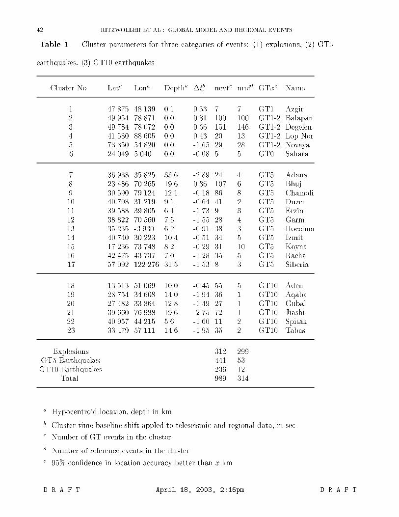
42 RITZWOLLER ET AL.: GLOBAL MODEL AND REGIONAL EVENTS
Table 1. Cluster parameters for three categories of events: (1) explosions, (2) GT5
earthquakes, (3) GT10 earthquakes.
Cluster No. Lata Lona Deptha �tb�
nevtc nrefd GTxe Name
1 47.875 48.139 0.1 0.53 7 7 GT1 Azgir2 49.954 78.871 0.0 0.81 100 100 GT1-2 Balapan3 49.784 78.072 0.0 0.66 151 146 GT1-2 Degelen4 41.580 88.605 0.0 0.43 20 13 GT1-2 Lop Nor5 73.350 54.820 0.0 -1.65 29 28 GT1-2 Novaya6 24.049 5.040 0.0 -0.08 5 5 GT0 Sahara
7 36.938 35.825 33.6 -2.89 24 4 GT5 Adana8 23.486 70.265 19.6 0.36 107 6 GT5 Bhuj9 30.590 79.124 12.1 -0.18 86 8 GT5 Chamoli10 40.798 31.219 9.1 -0.64 41 2 GT5 Duzce11 39.588 39.805 6.4 -1.73 9 3 GT5 Erzin12 38.822 70.560 7.5 -1.55 28 4 GT5 Garm13 35.235 -3.930 6.2 -0.91 38 3 GT5 Hoceima14 40.740 30.223 10.4 -0.51 34 5 GT5 Izmit15 17.236 73.748 8.2 -0.29 31 10 GT5 Koyna16 42.475 43.737 7.0 -1.28 35 5 GT5 Racha17 57.092 122.276 31.5 -1.53 8 3 GT5 Siberia
18 13.513 51.069 10.0 -0.45 55 5 GT10 Aden19 28.754 34.608 14.0 -1.94 36 1 GT10 Aqaba20 27.482 33.864 12.8 -1.49 27 1 GT10 Gubal21 39.660 76.988 19.6 -2.75 72 1 GT10 Jiashi22 40.957 44.215 5.6 -1.60 11 2 GT10 Spitak23 33.479 57.111 14.6 -1.95 35 2 GT10 Tabas
Explosions 312 299GT5 Earthquakes 441 53GT10 Earthquakes 236 12
Total 989 314
a Hypocentroid location, depth in km.
b Cluster time baseline shift appled to teleseismic and regional data, in sec.c Number of GT events in the cluster.
d Number of reference events in the cluster.e 95% con�dence in location accuracy better than x km.
D R A F T April 18, 2003, 2:16pm D R A F T

RITZWOLLER ET AL.: GLOBAL MODEL AND REGIONAL EVENTS 43
Table 2. Number of travel times in the groomed arrival time and the empirical phase
path anomaly data sets.
Groomed Arrival Times Empirical Path Anomalies
Pn P Pn P
Explosions 1521 477 121 35
GT5 8974 1380 558 108
GT10 3106 539 157 35
total 13601 2396 836 178
Table 3. Fit to empirical phase path anomalies for explosions.
CUB2.0 TH AK135
Cluster No. Name Na VRb RMSc Correld �t�e RMSc �t�
e
1 Azgir 18 87 0.94 0.88 1.17 2.58 1.99
2 Balapan 39 50 0.98 0.74 1.69 1.38 2.29
3 Degelen 14 57 0.98 0.67 0.54 1.49 1.61
4 Lop Nor 71 19 1.50 0.63 1.66 1.67 1.29
5 Novaya 14 79 0.70 0.83 0.15 1.53 2.90
averagef 65 1.02 0.75 1.04 1.73 2.02
a Number of measurements in cluster.
b Variance reduction in percent relative to AK135.c Rms-mis�t between observed and predicted travel times, in sec.
d Correlation between observed and predicted travel times.e Cluster time baseline shift applied to regional data alone, in sec.
f Average of absolute values.
D R A F T April 18, 2003, 2:16pm D R A F T
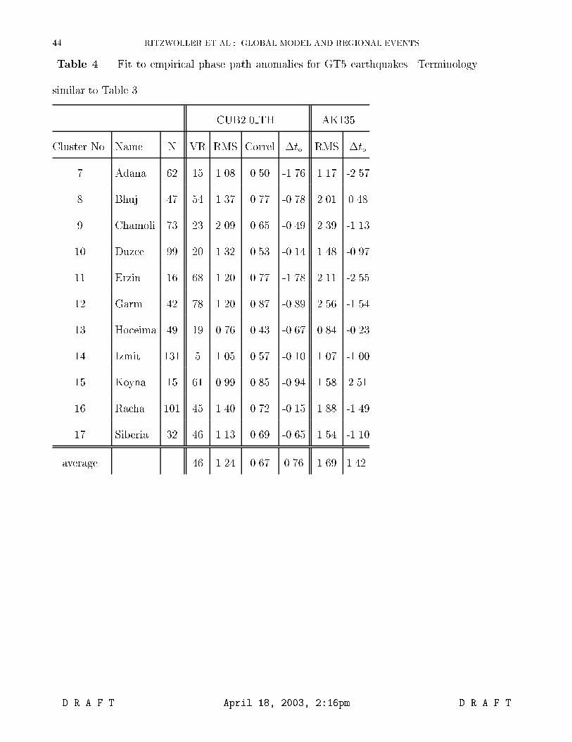
44 RITZWOLLER ET AL.: GLOBAL MODEL AND REGIONAL EVENTS
Table 4. Fit to empirical phase path anomalies for GT5 earthquakes. Terminology
similar to Table 3.
CUB2.0 TH AK135
Cluster No. Name N VR RMS Correl �t� RMS �t�
7 Adana 62 15 1.08 0.50 -1.76 1.17 -2.57
8 Bhuj 47 54 1.37 0.77 -0.78 2.01 0.48
9 Chamoli 73 23 2.09 0.65 -0.49 2.39 -1.13
10 Duzce 99 20 1.32 0.53 -0.14 1.48 -0.97
11 Erzin 16 68 1.20 0.77 -1.78 2.11 -2.55
12 Garm 42 78 1.20 0.87 -0.89 2.56 -1.54
13 Hoceima 49 19 0.76 0.43 -0.67 0.84 -0.23
14 Izmit 131 5 1.05 0.57 -0.10 1.07 -1.00
15 Koyna 15 61 0.99 0.85 -0.94 1.58 2.51
16 Racha 101 45 1.40 0.72 -0.15 1.88 -1.49
17 Siberia 32 46 1.13 0.69 -0.65 1.54 -1.10
average 46 1.24 0.67 0.76 1.69 1.42
D R A F T April 18, 2003, 2:16pm D R A F T
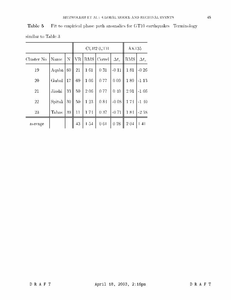
RITZWOLLER ET AL.: GLOBAL MODEL AND REGIONAL EVENTS 45
Table 5. Fit to empirical phase path anomalies for GT10 earthquakes. Terminology
similar to Table 3.
CUB2.0 TH AK135
Cluster No. Name N VR RMS Correl �t� RMS �t�
19 Aqaba 80 21 1.61 0.31 -0.11 1.81 -0.26
20 Gubal 17 69 1.06 0.77 0.09 1.89 -1.13
21 Jiashi 33 50 2.06 0.77 0.40 2.91 -1.66
22 Spitak 30 50 1.23 0.84 -0.08 1.74 -1.40
23 Tabas 39 11 1.74 0.37 -0.71 1.84 -2.58
average 43 1.54 0.61 0.28 2.04 1.41
D R A F T April 18, 2003, 2:16pm D R A F T

46 RITZWOLLER ET AL.: GLOBAL MODEL AND REGIONAL EVENTS
Table 6. Location results for nuclear explosions.
CUB2.0 TH AK135
Cluster No. Name Eventsa Stationsb Errorc RMSd Errorc RMSd
1 Azgir 6 19 4.2 1.08 24.0 1.49
2 Balapan 10 25 3.9 1.10 11.2 1.22
3 Degelen 3 18 3.1 1.01 12.0 1.36
4 Lop Nor 16 45 6.1 1.22 9.6 1.49
5 Novaya 3 15 8.0 1.03 13.6 1.57
overalle 38 24 5.1 1.09 14.1 1.43
a Number of events with open azimuth < 180� and � 5 stations.
b Median number of stations.c Average distance from estimated to GT location, in km.
d Rms di�erence between observed and predicted travel times, in sec.e Total or average of cluster values.
D R A F T April 18, 2003, 2:16pm D R A F T
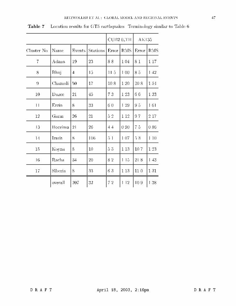
RITZWOLLER ET AL.: GLOBAL MODEL AND REGIONAL EVENTS 47
Table 7. Location results for GT5 earthquakes. Terminology similar to Table 6.
CUB2.0 TH AK135
Cluster No. Name Events Stations Error RMS Error RMS
7 Adana 19 23 8.8 1.04 8.1 1.17
8 Bhuj 4 15 11.5 1.00 8.5 1.42
9 Chamoli 50 17 10.8 1.20 20.8 1.54
10 Duzce 21 45 7.3 1.23 6.6 1.33
11 Erzin 8 33 6.0 1.29 9.5 1.61
12 Garm 26 21 5.2 1.12 9.7 2.17
13 Hoceima 21 26 4.4 0.90 7.5 0.86
14 Izmit 8 116 5.1 1.07 5.3 1.10
15 Koyna 8 10 5.5 1.13 10.7 1.23
16 Racha 34 20 8.2 1.15 21.8 1.43
17 Siberia 8 33 6.3 1.13 11.0 1.31
overall 207 32 7.2 1.12 10.9 1.38
D R A F T April 18, 2003, 2:16pm D R A F T
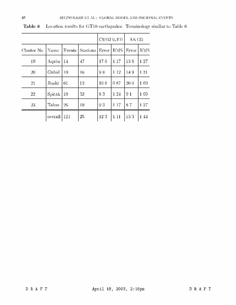
48 RITZWOLLER ET AL.: GLOBAL MODEL AND REGIONAL EVENTS
Table 8. Location results for GT10 earthquakes. Terminology similar to Table 6.
CUB2.0 TH AK135
Cluster No. Name Events Stations Error RMS Error RMS
19 Aqaba 14 47 17.6 1.17 13.8 1.27
20 Gubal 10 16 9.8 1.12 14.9 1.31
21 Jiashi 61 12 16.6 0.87 20.0 1.69
22 Spitak 10 32 8.3 1.24 9.1 1.69
23 Tabas 26 19 9.3 1.17 8.7 1.27
overall 121 25 12.3 1.11 13.3 1.44
D R A F T April 18, 2003, 2:16pm D R A F T
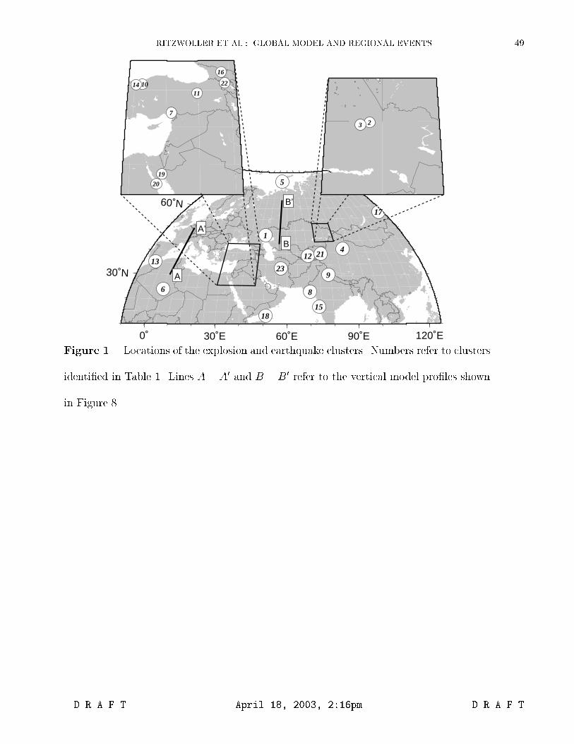
RITZWOLLER ET AL.: GLOBAL MODEL AND REGIONAL EVENTS 49
0˚ 30˚E 60˚E 90˚E 120˚E
30˚N
60˚N
1
8
9
1213
21
15
4
5
6
18
17
23
7
19
1011
20
14
16
22
23
B
B’
A
A’
Figure 1. Locations of the explosion and earthquake clusters. Numbers refer to clusters
identi�ed in Table 1. Lines A� A0 and B �B0 refer to the vertical model pro�les shown
in Figure 8.
D R A F T April 18, 2003, 2:16pm D R A F T
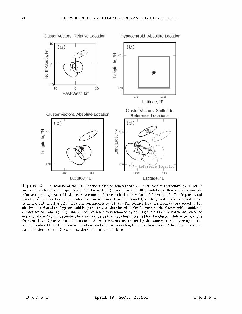
50 RITZWOLLER ET AL.: GLOBAL MODEL AND REGIONAL EVENTS
10
0
-10-10 0 10
12
3
4
East-West, km
Nor
th-S
outh
, km
Cluster Vectors, Relative Location
(a)
12
3
4
73.2 73.3
47.0
47.1
Long
itude
, °N
Latitude, °E
Cluster Vectors, Absolute Location
(c)
47.1
73.2 73.3
47.0
Long
itude
, °N
Latitude, °E
Hypocentroid, Absolute Location
(b)
47.1
73.2 73.3
47.0
Long
itude
, °N
Latitude, °E
12
3
4
Cluster Vectors, Shifted toReference Locations
= Reference Location
(d)
Figure 2. Schematic of the HDC analysis used to generate the GT data base in this study. (a) Relativelocations of cluster event epicenters (\cluster vectors") are shown with 90% con�dence ellipses. Locations arerelative to the hypocentroid, the geometric mean of current absolute locations of all events. (b) The hypocentroid(solid star) is located using all cluster event arrival time data (appropriately shifted) as if it were an earthquake,using the 1-D model AK135. The box corresponds to (a). (c) The relative locations from (a) are added to theabsolute location of the hypocentroid in (b) to give absolute locations for all events in the cluster, with con�denceellipses scaled from (a). (d) Finally, the location bias is removed by shifting the cluster to match the referenceevent locations (from independent local seismic data) that have been obtained for this cluster. Reference locationsfor event 1 and 3 are shown by open stars. All cluster events are shifted by the same vector, the average of theshifts calculated from the reference locations and the corresponding HDC locations in (c). The shifted locationsfor all cluster events in (d) compose the GT location data base.
D R A F T April 18, 2003, 2:16pm D R A F T
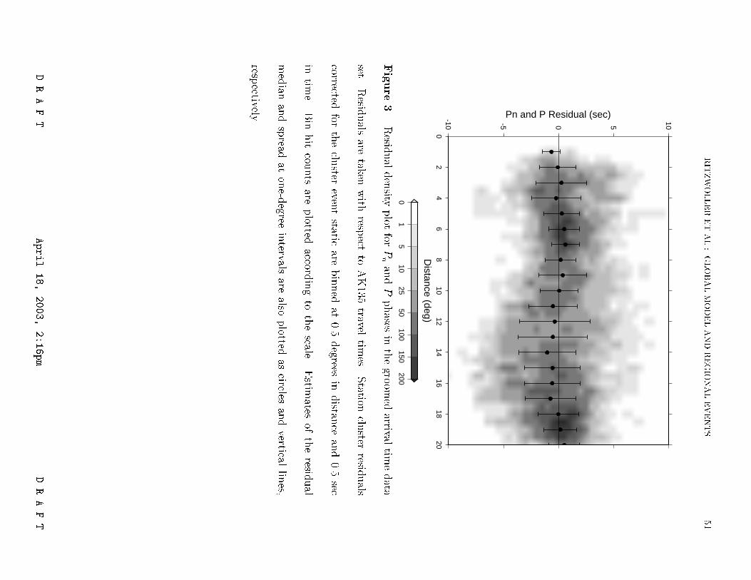
RITZWOLLERETAL.:GLOBALMODELANDREGIONALEVENTS
51
-10 -5 0 5 10
Pn and P Residual (sec)
02
46
810
1214
1618
20
Distance (deg)
01
510
2550
100150
200
Figure3.
Resid
ualdensity
plot
forPnandPphases
inthegro
omed
arrivaltim
edata
set.Resid
uals
aretaken
with
respect
toAK135
traveltim
es.Station
cluster
residuals
correctedfor
theclu
stereven
tstatic
arebinned
at0.5
degrees
indistan
ceand0.5
sec
intim
e.Bin
hit
counts
areplotted
accordingto
thescale.
Estim
atesof
theresid
ual
median
andspread
atone-d
egreeintervals
arealso
plotted
ascircles
andvertical
lines,
respectively.
DR
AF
TApril
18,
2003,
2:16pm
DRA
FT

52 RITZWOLLER ET AL.: GLOBAL MODEL AND REGIONAL EVENTS
-8
-6
-4
-2
0
2
4
6
8
Pat
h C
orre
ctio
n (s
ec)
0 2 4 6 8 10 12 14 16 18 20
Distance (deg)
-10
-5
0
5
10
15
Red
uced
Tra
vel T
ime
(sec
)
14 16 18 20
Distance (deg)
(a) (b)
Figure 4. Reduced Pn (white) and P (black) empirical phase path anomalies plotted
as the median and spread estimates with respect to distance. Travel times are corrected
for cluster time baseline shifts. (a) Results are presented as residuals with respect to the
AK135 travel times. (b) Results are presented near the Pn=P cross-over as reduced travel
times (relative to 8.0 km/s). AK135 predicted Pn and P travel time branches are also
shown.
D R A F T April 18, 2003, 2:16pm D R A F T
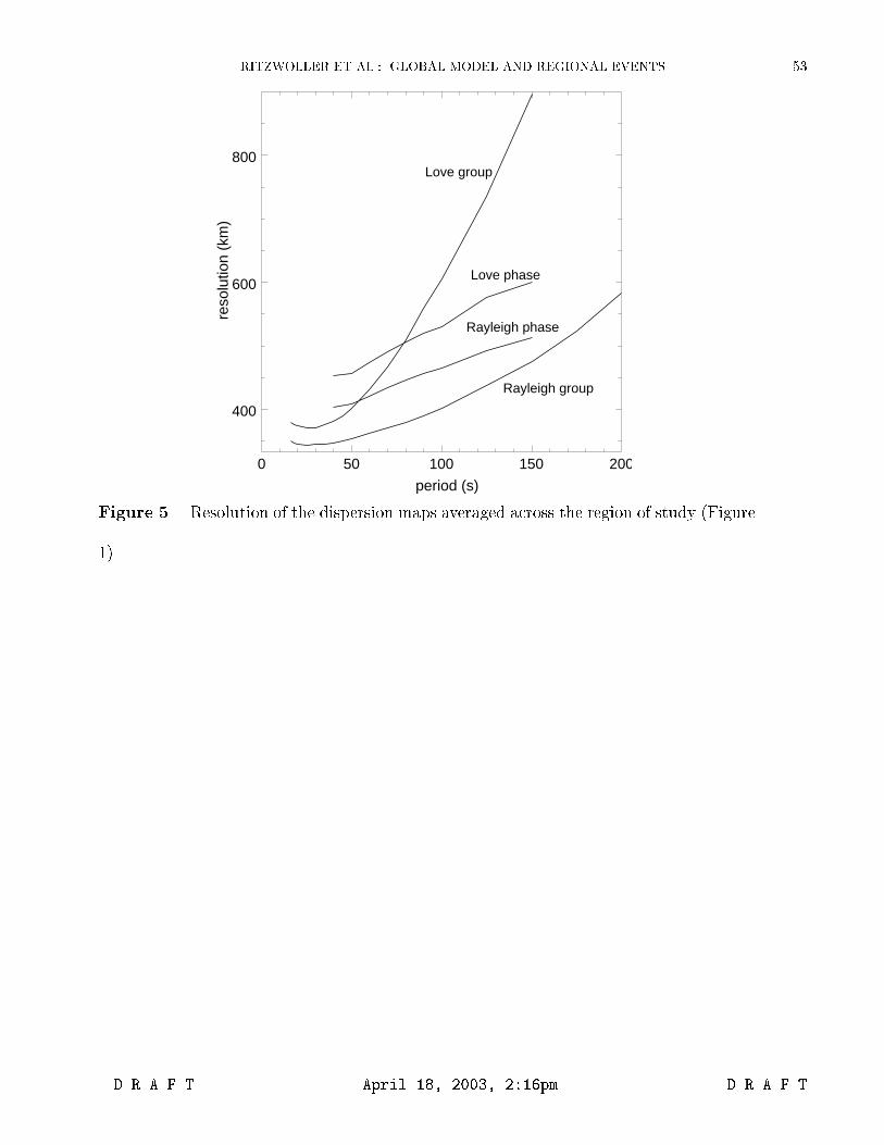
RITZWOLLER ET AL.: GLOBAL MODEL AND REGIONAL EVENTS 53
0 50 100 150 200
400
600
800
period (s)
reso
lutio
n (k
m)
Rayleigh group
Rayleigh phase
Love phase
Love group
Figure 5. Resolution of the dispersion maps averaged across the region of study (Figure
1).
D R A F T April 18, 2003, 2:16pm D R A F T
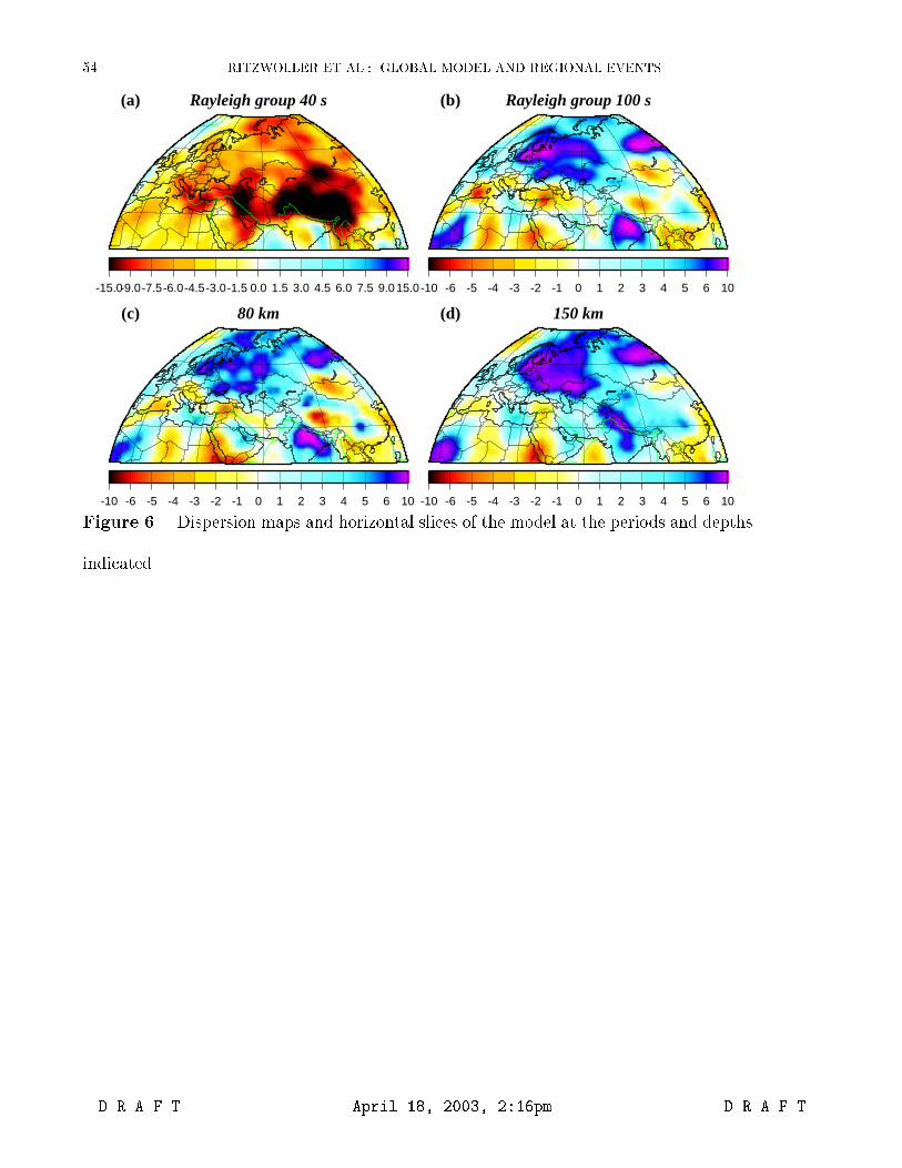
54 RITZWOLLER ET AL.: GLOBAL MODEL AND REGIONAL EVENTS
-15.0-9.0-7.5-6.0-4.5-3.0-1.5 0.0 1.5 3.0 4.5 6.0 7.5 9.0 15.0-10 -6 -5 -4 -3 -2 -1 0 1 2 3 4 5 6 10
-10 -6 -5 -4 -3 -2 -1 0 1 2 3 4 5 6 10 -10 -6 -5 -4 -3 -2 -1 0 1 2 3 4 5 6 10
Rayleigh group 40 s Rayleigh group 100 s
80 km 150 km
(a) (b)
(c) (d)
Figure 6. Dispersion maps and horizontal slices of the model at the periods and depths
indicated.
D R A F T April 18, 2003, 2:16pm D R A F T

RITZWOLLER ET AL.: GLOBAL MODEL AND REGIONAL EVENTS 55
300
200
100
0
dept
h (k
m)
3.0 3.5 4.0 4.5 5.0
S-wave velocity (km/s)
300
200
100
0
dept
h (k
m)
3.0 3.5 4.0 4.5 5.0
S-wave velocity (km/s)
300
200
100
0
dept
h (k
m)
3.0 3.5 4.0 4.5 5.0
S-wave velocity (km/s)
3
4
5
velo
city
(km
/s)
20 50 100 200
period (s)
Rayleigh phase
Love phase
Love group
Rayleigh group
a) b)
c) d)
Figure 7. (a) Observed dispersion curves at a point in Iran (30�N, 60�E). The black lines
are observations derived from the dispersion maps and the grey shaded zones represent
the range of dispersion curves from the the ensemble of acceptable models shown in
(b). Inversion results for three data sets: (b) simultaneous inversion of group and phase
speeds (CUB2.0), (c) group speed alone, and (d) phase speed alone. The full width of the
ensemble of acceptable models is indicated, where vsh is dark grey and vsv is light grey.
D R A F T April 18, 2003, 2:16pm D R A F T

56 RITZWOLLER ET AL.: GLOBAL MODEL AND REGIONAL EVENTS
dVs/Vs (%)
400
300
200
100
0
dept
h (k
m)
30 40 50latitude
A A'a)
400
300
200
100
0
dept
h (k
m)
50 60latitude
B B'b)
-7 -5 -3 -1 1 3 5 7
Figure 8. Vertical slices of the vs model from CUB2.0 plotted as percent deviation
from AK135. Locations of the pro�les are shown in Figure 1.
400
350
300
250
200
150
100
50
dept
h (k
m)
4.0 4.5 5.0Vs (km/s)
dept
h (k
m)
Vs (km/s)
400
350
300
250
200
150
100
50
4.0 4.5 5.0
Vp (km/s) scaling factor
a) b)
7.3 7.6 7.9 8.2 8.5 8.8 9.1 1.2 1.4 1.6 1.8 2.0 2.2
Figure 9. (a) Grid used for the thermoelastic vs to vp conversion. (b) The thermoelastic
conversion presented as the logarithmic scaling factor d ln vs=d ln vp. The solid black line
is vs from the 1-D model AK135 and the dashed line is vs converted from AK135 vp by
the thermoelastic conversion.
D R A F T April 18, 2003, 2:16pm D R A F T

RITZWOLLER ET AL.: GLOBAL MODEL AND REGIONAL EVENTS 57
7.5 8 8.5 9 9.5400
350
300
250
200
150
100
50
0
Vp (km/s)
dept
h (k
m)
7.5 8 8.5 9 9.5400
350
300
250
200
150
100
50
0
Vp (km/s)
dept
h (k
m)
a) b)A-A' B-B'
Figure 10. vp model at the mid-points of pro�les (a) A�A0 and (b) B�B0 from Figures
1 and 8. The solid line represents the thermoelastic conversion from vs (i.e., CUB2.0 TH)
and the dashed line is from the empirical scaling relation d ln vs=d ln vp = 2:0 in which
AK135 is used as the reference (i.e., CUB2.0 EMP).
D R A F T April 18, 2003, 2:16pm D R A F T
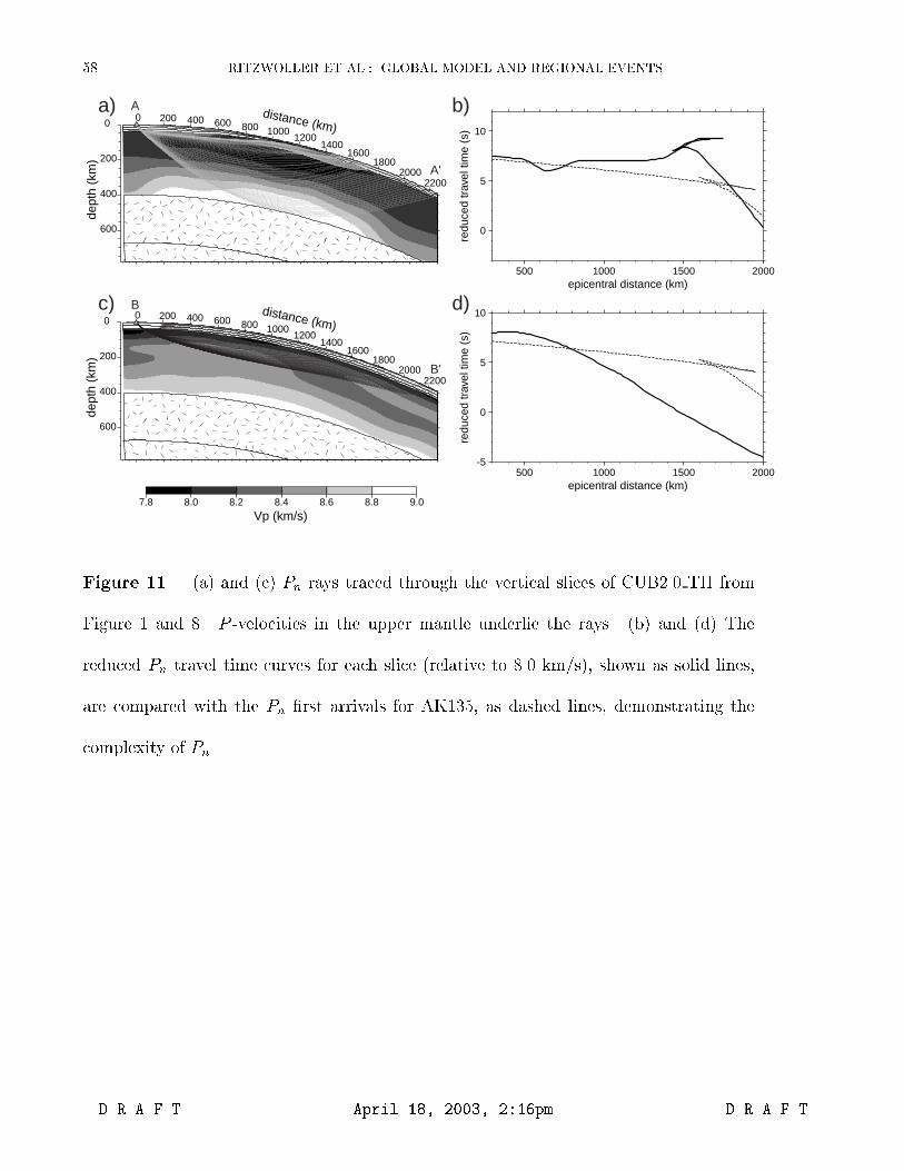
58 RITZWOLLER ET AL.: GLOBAL MODEL AND REGIONAL EVENTS
Vp (km/s)
0
5
10
redu
ced
trav
el ti
me
(s)
500 1000 1500 2000epicentral distance (km)
-5
0
5
10
redu
ced
trav
el ti
me
(s)
500 1000 1500 2000epicentral distance (km)
7.8 8.0 8.2 8.4 8.6 8.8 9.0
600
400
200
0
dept
h (k
m)
800 10001200
14001600
18002000
2200
0 200 400 600distance (km)
A
A'
600
400
200
0
dept
h (k
m)
800 10001200
14001600
18002000
2200
0 200 400 600distance (km)
B
B'
a) b)
c) d)
Figure 11. (a) and (c) Pn rays traced through the vertical slices of CUB2.0 TH from
Figure 1 and 8. P -velocities in the upper mantle underlie the rays. (b) and (d) The
reduced Pn travel time curves for each slice (relative to 8.0 km/s), shown as solid lines,
are compared with the Pn �rst arrivals for AK135, as dashed lines, demonstrating the
complexity of Pn.
D R A F T April 18, 2003, 2:16pm D R A F T

RITZWOLLER ET AL.: GLOBAL MODEL AND REGIONAL EVENTS 59
Pn time difference (s)
200 600 1000 1400 1800-4
-3
-2
-1
0
1
Pn
time
diffe
renc
e (s
)
distance (km)
20˚E
40˚E60˚E
20˚N
30˚N
40˚N
50˚N
60˚N
a) b)
-2.5 -2.0 -1.5 -1.0 -0.5 0.0 0.5 1.0
Figure 12. E�ect of the vs to vp conversion on Pn travel times. (a) Di�erence be-
tween Pn travel times from CUB2.0 TH and CUB2.0 EMP centered on stations KIV
(Kislovodsk, Russia). Positive values mean CUB2.0 TH travel times are faster than those
from CUB2.0 EMP. (b) Solid line shows the Pn travel time di�erence for pro�le B � B0
and the dashed line for A�A0 from Figures 1 and 8. One standard deviation errors bars
show the geographical average across the region of study (Figure 1).
D R A F T April 18, 2003, 2:16pm D R A F T
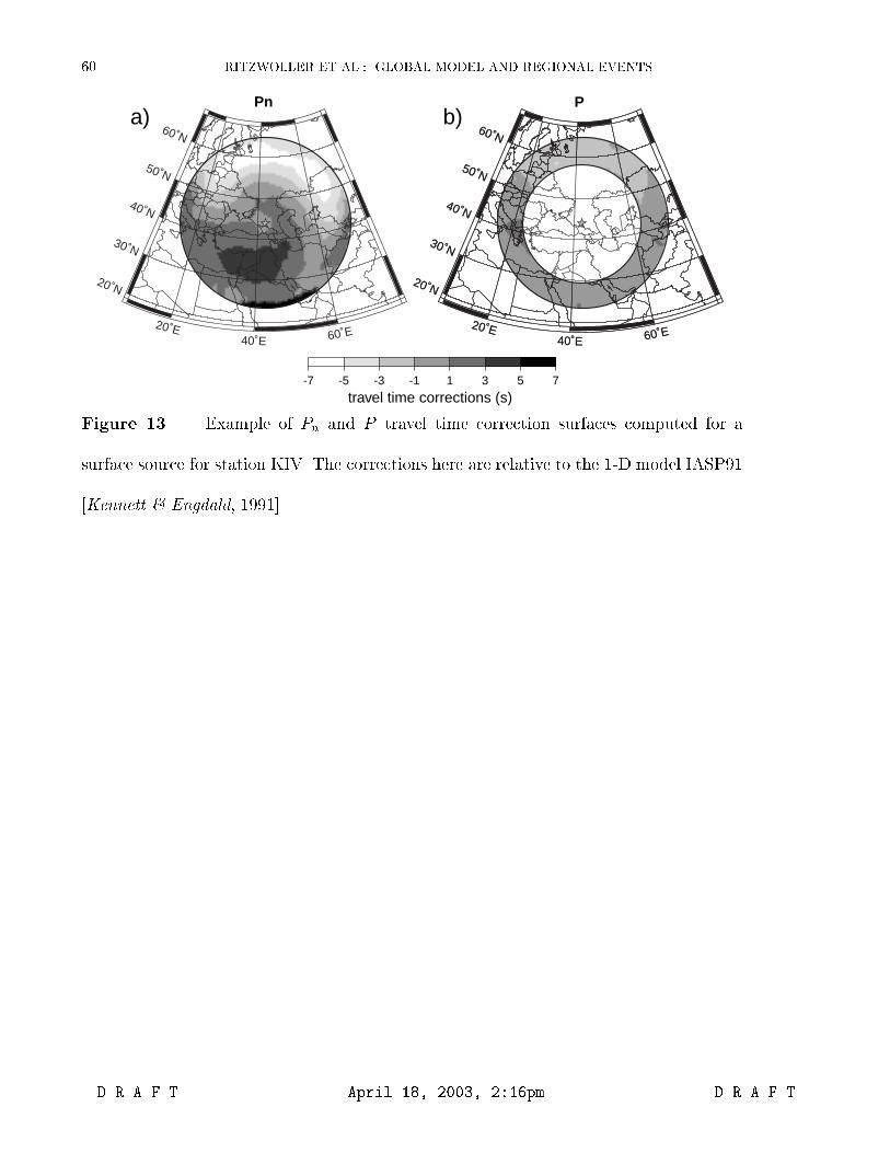
60 RITZWOLLER ET AL.: GLOBAL MODEL AND REGIONAL EVENTS
-7 -5 -3 -1 1 3 5 7
travel time corrections (s)
Pn Pa) b)
20 E40 E 60 E
20 N
30 N
40 N
50 N
60 N
20 E40 E 60 E
20 N
30 N
40 N
50 N
60 N
20 E40 E 60 E
20 N
30 N
40 N
50 N
60 N
Figure 13. Example of Pn and P travel time correction surfaces computed for a
surface source for station KIV. The corrections here are relative to the 1-D model IASP91
[Kennett & Engdahl, 1991].
D R A F T April 18, 2003, 2:16pm D R A F T

RITZWOLLER ET AL.: GLOBAL MODEL AND REGIONAL EVENTS 61
60 E80 E 100 E
10 N
20 N
30 N
40 N
50 N
20 E40 E 60 E
20 N
30 N
40 N
50 N
60 N
-7 -5 -3 -1 1 3 5 7travel time correction relative to AK135 (s)
a) b)
c) d)
Azgir
20 E40 E 60 E
80 E
30 N
40 N
50 N
60 N
70 N
Chamoli
60 E80 E 100 E
120 E
20 N
30 N
40 N
50 N
60 N
Lop Nor
Racha
Figure 14. Cluster-centered travel time correction surfaces for four cluster regions.
The colored contours are the predictions from the 3-D model CUB2.0 TH referenced to
the travel time from the 1-D model AK135. The symbols are the empirical phase path
anomalies, color-coded similarly to the model predictions. The cluster time baseline shift
is indicated in Tables 3 and 4. (a) and (b) are explosions in the Azgir and Lop Nor clusters
and (c) and (d) are earthquakes in the Chamoli and Racha clusters, respectively.
D R A F T April 18, 2003, 2:16pm D R A F T

62 RITZWOLLER ET AL.: GLOBAL MODEL AND REGIONAL EVENTS
a) b)
c) d)
-5
0
53D
mod
el p
redi
ctio
n(s)
-5 0 5empirical path anomalies (s)
-5
0
5
3D m
odel
pre
dict
ion(
s)
-5 0 5empirical path anomalies (s)
-5
0
5
3D m
odel
pre
dict
ion(
s)
-5 0 5empirical path anomalies (s)
-5
0
53D
mod
el p
redi
ctio
n(s)
-5 0 5empirical path anomalies (s)
Azgir Lop Nor
Chamoli Racha
Figure 15. Comparison between the P and Pn travel times predicted by the 3-D model
CUB2.0 TH and the empirical phase path anomalies for the four event clusters shown in
Figure 14. The empirical path anomalies are on the horizontal axis, paired with the model
predictions on the vertical axis. Circles are Pn and triangles are P . Phases have been
re-identi�ed using the 3-D model; bars link phases originally identi�ed with the 1-D model
AK135 (shaded gray) to the re-identi�ed phases (unshaded). The cluster time baseline
shifts listed in Tables 3 and 4 have been applied. The dashed lines mark the location of
�3 sec residuals.
D R A F T April 18, 2003, 2:16pm D R A F T
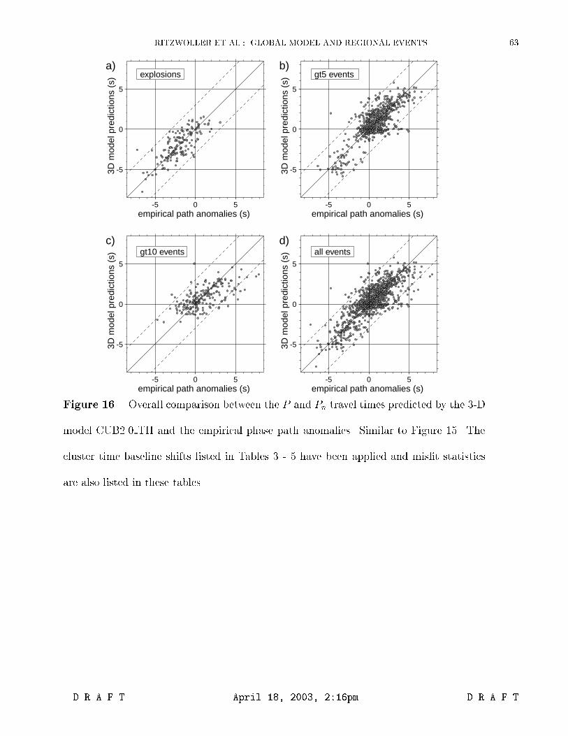
RITZWOLLER ET AL.: GLOBAL MODEL AND REGIONAL EVENTS 63
-5
0
5
3D m
odel
pre
dict
ions
(s)
-5 0 5empirical path anomalies (s)
-5
0
5
3D m
odel
pre
dict
ions
(s)
-5 0 5empirical path anomalies (s)
-5
0
5
3D m
odel
pre
dict
ions
(s)
-5 0 5empirical path anomalies (s)
-5
0
5
3D m
odel
pre
dict
ions
(s)
-5 0 5empirical path anomalies (s)
a) b)
c) d)
explosions
all events
gt5 events
gt10 events
Figure 16. Overall comparison between the P and Pn travel times predicted by the 3-D
model CUB2.0 TH and the empirical phase path anomalies. Similar to Figure 15. The
cluster time baseline shifts listed in Tables 3 - 5 have been applied and mis�t statistics
are also listed in these tables.
D R A F T April 18, 2003, 2:16pm D R A F T
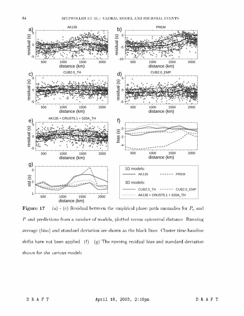
64 RITZWOLLER ET AL.: GLOBAL MODEL AND REGIONAL EVENTS
AK135 PREM
CUB2.0_TH CUB2.0_EMP
AK135 + CRUST5.1 + S20A_TH
-5
0
5re
sidu
al (
s)
500 1000 1500 2000distance (km)
-5
0
5
resi
dual
(s)
500 1000 1500 2000distance (km)
-5
0
5
resi
dual
(s)
500 1000 1500 2000distance (km)
-5
0
5
resi
dual
(s)
500 1000 1500 2000distance (km)
-10
-5
0
resi
dual
(s)
500 1000 1500 2000distance (km)
-4
-2
0
bias
(s)
500 1000 1500 2000distance (km)
1
2
3
std
(s)
500 1000 1500 2000distance (km)
PREMAK135
CUB2.0_TH CUB2.0_EMP
AK135 + CRUST5.1 + S20A_TH
1D models:
3D models:
a) b)
g)
e) f)
c) d)
Figure 17. (a) - (e) Residual between the empirical phase path anomalies for Pn and
P and predictions from a number of models, plotted versus epicentral distance. Running
average (bias) and standard deviation are shown as the black lines. Cluster time baseline
shifts have not been applied. (f) - (g) The running residual bias and standard deviation
shown for the various models.
D R A F T April 18, 2003, 2:16pm D R A F T

RITZWOLLER ET AL.: GLOBAL MODEL AND REGIONAL EVENTS 65
41o24'
41o36'
41o48'
88o36' 88o48' 89o00'
1.2
1.4
1.4
1.6
1.6
1.6
1.8
1.8
1.8
2
2
2
2.2 2.4
2.6
22 km
GT location
1D location
PDE location
3D location
Figure 18. Contours of rms-mis�t using the 3-D model CUB2.0 TH for a grid of
hypothesized epicenters for an explosion at the Lop Nor test site (May 26, 1990; 54
reporting stations). Units are seconds. The GT1-2 location is indicated with a star, the
best-�t locations using the 3-D model CUB2.0 TH and the 1-D model AK135 are shown
with a triangle and a circle, respectively, and the PDE location is shown with a diamond.
D R A F T April 18, 2003, 2:16pm D R A F T

66 RITZWOLLER ET AL.: GLOBAL MODEL AND REGIONAL EVENTS
42o12'
42o24'
42o36'
42o48'
43o12' 43o36' 44o00' 44o24'41o24'
41o36'
41o48'
88o12' 88o24' 88o36' 88o48'
41o24'
41o36'
41o48'
88o12' 88o24' 88o36' 88o48'
42o12'
42o24'
42o36'
42o48'
43o12' 43o36' 44o00' 44o24'
11km
11km
11km
11km
(a)
(c)
(b)
(d)
Lop Nor Racha
3-D
1-D
GT location 3D location 1D location
Figure 19. Mislocation vectors from two event clusters for (left column) explosions
on the Lop Nor test site and (right column) earthquakes near Racha, Georgia. (a) and
(b) 3-D model (CUB2.0 TH) locations. (c) and (d) 1-D model (AK135) locations. Stars
mark GT locations, triangles and circles are 3-D and 1-D model locations, respectively.
D R A F T April 18, 2003, 2:16pm D R A F T

RITZWOLLER ET AL.: GLOBAL MODEL AND REGIONAL EVENTS 67
a) Lop Nor b) Lop Nor c) Racha d) Racha
50
100
150
200
250op
en a
zim
uth
5 10 15 20 25number of stations
0 4 8 12 16 20location error (km)
50
100
150
200
250
open
azi
mut
h
5 10 15 20 25number of stations
50
100
150
200
250
open
azi
mut
h
5 10 15 20 25number of stations
50
100
150
200
250
open
azi
mut
h
5 10 15 20 25number of stations
Figure 20. Mislocation using the 3-D model CUB2.0 TH, presented as a function of
number of stations and open azimuth, determined by randomly choosing subsets of the
reported travel times for four events: (a) Lop Nor, May 26, 1990; (b) Lop Nor, Sept 25,
1992; (c) Racha, May 3, 1991; (d) Racha, July 4, 1991.
D R A F T April 18, 2003, 2:16pm D R A F T

68 RITZWOLLER ET AL.: GLOBAL MODEL AND REGIONAL EVENTS
5 10 15 200
5
10
15
20
25
5 10 15 200
5
10
15
20
25(a) Explosions (b) GT5
5 10 15 2060
70
80
90
100(c)
number of stations number of stations
number of stations
explosions
GT5
AK135AK135
CUB2.0_THCUB2.0_THlo
catio
n er
ror
(km
)
loca
tion
erro
r (k
m)
perc
ent i
mpr
oved
Figure 21. Location error for the 3-D and 1-D models, plotted as a function of the
number of reporting stations, determined by randomly choosing subsets of the reported
travel times in which open-azimuth is constrained to be less than 180�. (a) and (b)
Average (solid lines) and standard deviation (dashed lines) are shown for explosions and
GT5 earthquakes for CUB2.0 TH (black lines) and AK135 (grey lines). (c) Percent of the
events for which the location error is smaller using the 3-D model than the 1-D model for
explosions (solid line) and GT5 earthquakes (dashed line).
D R A F T April 18, 2003, 2:16pm D R A F T