SO.2d ----, 2008 WL 5411659 (Fla. 1 - Florida Bar Business ...

Ramin Shamshiri ABE 6986, HW #1 Due 09/03/08
Homework #1
Due 09/03/08
ABE 6986
Ramin Shamshiri
UFID # 90213353
1- Calculate the ratio W/H for each age.
Answer:
Table 1: Dependence of height (H) and weight (W) on age (t) for males in Belgium.
yr H W W/H
0 0.5 3.2 6.4
1 0.7 10 14.28571
2 0.8 12 15
3 0.86 13.21 15.36047
4 0.93 15.07 16.2043
5 0.99 16.7 16.86869
6 1.05 18.04 17.18095
7 1.11 20.16 18.16216
8 1.17 22.26 19.02564
9 1.23 24.09 19.58537
10 1.28 26.12 20.40625
11 1.33 27.85 20.93985
12 1.36 31 22.79412
13 1.4 35.32 25.22857
14 1.49 40.5 27.18121
15 1.56 46.41 29.75
16 1.61 53.39 33.16149
17 1.67 57.4 34.37126
18 1.7 61.26 36.03529
19 1.71
20 1.71 65 38.0117
25 1.72 68.29 39.70349
30 1.72 68.9 40.05814
40 1.71 68.81 40.23977
50 1.67 67.45 40.38922
60 1.64 65.5 39.93902
70 1.62 63.03 38.90741
80 1.61 61.22 38.02484
Ramin Shamshiri ABE 6986, HW #1 Due 09/03/08
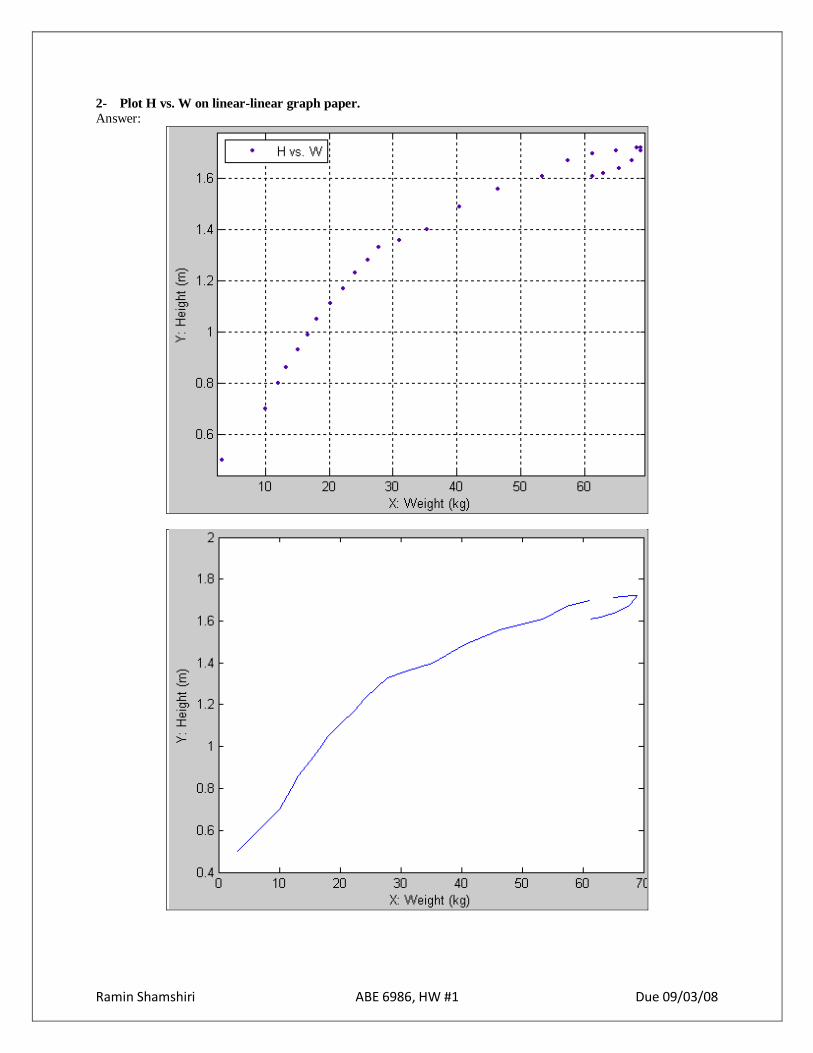
2- Plot H vs. W on linear-linear graph paper.
Answer:

Ramin Shamshiri ABE 6986, HW #1 Due 09/03/08
3- Plot W/H vs. W on linear-linear graph paper.
Answer:
Ramin Shamshiri ABE 6986, HW #1 Due 09/03/08
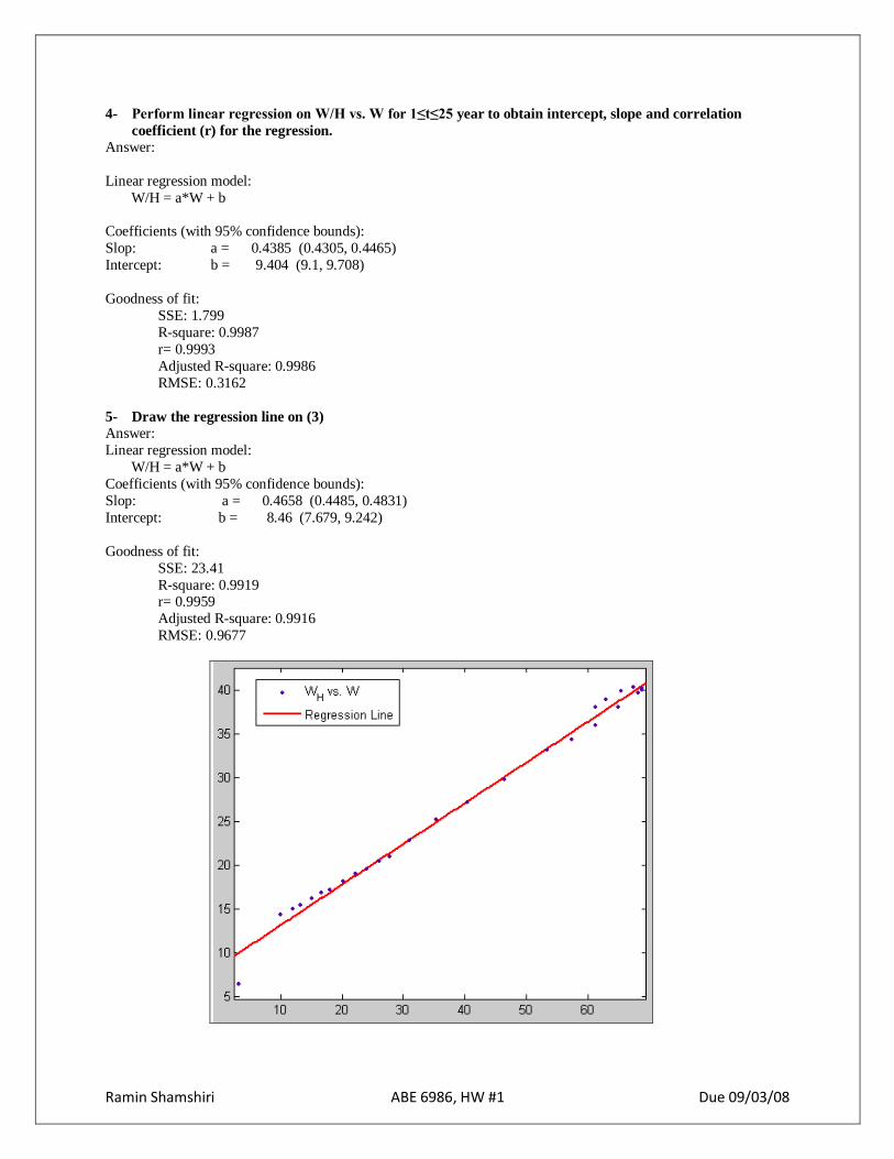
4- Perform linear regression on W/H vs. W for 1≤t≤25 year to obtain intercept, slope and correlation
coefficient (r) for the regression.
Answer:
Linear regression model:
W/H = a*W + b
Coefficients (with 95% confidence bounds):
Slop: a = 0.4385 (0.4305, 0.4465)
Intercept: b = 9.404 (9.1, 9.708)
Goodness of fit:
SSE: 1.799
R-square: 0.9987
r= 0.9993
Adjusted R-square: 0.9986
RMSE: 0.3162
5- Draw the regression line on (3)
Answer:
Linear regression model:
W/H = a*W + b
Coefficients (with 95% confidence bounds):
Slop: a = 0.4658 (0.4485, 0.4831)
Intercept: b = 8.46 (7.679, 9.242)
Goodness of fit:
SSE: 23.41
R-square: 0.9919 r= 0.9959
Adjusted R-square: 0.9916
RMSE: 0.9677
Ramin Shamshiri ABE 6986, HW #1 Due 09/03/08
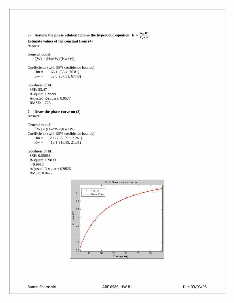
6- Assume the phase relation follows the hyperbolic equation: 𝑯 =𝑯𝒎.𝑾
𝑲𝒘+𝑾.
Estimate values of the constant from (4)
Answer:
General model:
f(W) = (Hm*W)/(Kw+W)
Coefficients (with 95% confidence bounds):
Hm = 66.1 (55.4, 76.81)
Kw = 52.5 (37.51, 67.48)
Goodness of fit:
SSE: 53.47
R-square: 0.9599
Adjusted R-square: 0.9577
RMSE: 1.723
7- Draw the phase curve on (2) Answer:
General model:
f(W) = (Hm*W)/(Kw+W)
Coefficients (with 95% confidence bounds):
Hm = 2.177 (2.093, 2.261)
Kw = 19.1 (16.89, 21.31)
Goodness of fit:
SSE: 0.05688
R-square: 0.9833
r=0.9916 Adjusted R-square: 0.9826
RMSE: 0.0477
Ramin Shamshiri ABE 6986, HW #1 Due 09/03/08
8- Discuss your results.
Does the phase equation appear reasonable for these data? How would you justify the phase relation Eq. (1)?
Answer:
From the result, we can see that the correlation coefficient (r) in the linear model is close to 1 which shows a very good fit. In the other side, the phase equation seems to fit most of the data spots on its curve. The question is that
which equation, the linear or the phase is more reasonable in this case. If the accuracy is not a big issue, I think the
linear model is enough in this case, however for a sensitive case, if the higher accuracy is required; a more complex
equation such as hyperbolic equation is a better representative of the correlation. Results show that up to a certain
age point, the data lie on the phase curve, but after that the phase equation model does not perform a good
prediction. A question that comes to my mind is that, can we compare the goodness of fit for two models? For
example, here we have a linear and a hyperbolic model with r=0.9959 and r=0.9916 respectively. Are we allowed to
compare these two values to conclude which one is a better prediction model?
Ramin Shamshiri ABE 6986, HW #2 Due 09/10/08
Homework #2
Due 09/10/08
ABE 6986
Ramin Shamshiri
UFID # 90213353
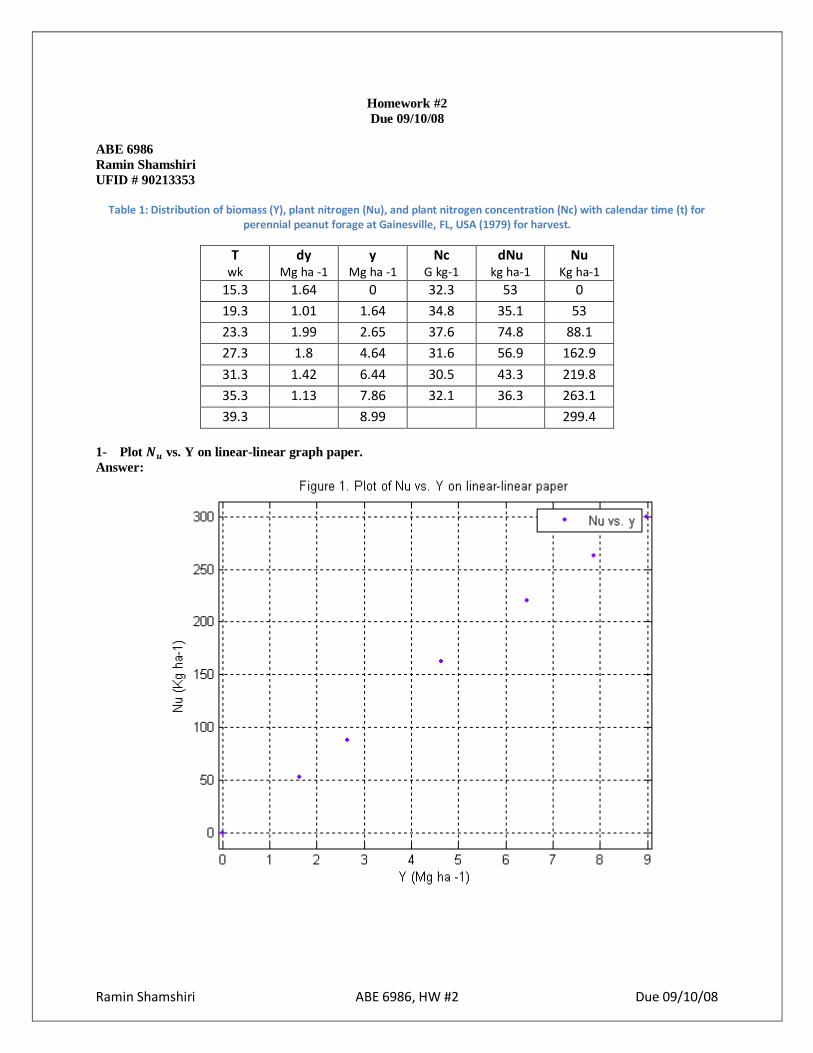
Table 1: Distribution of biomass (Y), plant nitrogen (Nu), and plant nitrogen concentration (Nc) with calendar time (t) for
perennial peanut forage at Gainesville, FL, USA (1979) for harvest.
T wk
dy Mg ha -1
y Mg ha -1
Nc G kg-1
dNu kg ha-1
Nu Kg ha-1
15.3 1.64 0 32.3 53 0
19.3 1.01 1.64 34.8 35.1 53
23.3 1.99 2.65 37.6 74.8 88.1
27.3 1.8 4.64 31.6 56.9 162.9
31.3 1.42 6.44 30.5 43.3 219.8
35.3 1.13 7.86 32.1 36.3 263.1
39.3 8.99 299.4
1- Plot 𝑵𝒖 vs. Y on linear-linear graph paper.
Answer:
Ramin Shamshiri ABE 6986, HW #2 Due 09/10/08
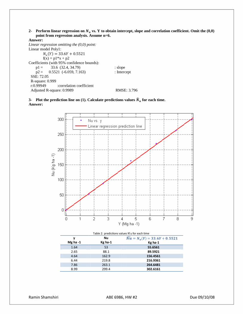
2- Perform linear regression on 𝑵𝒖 vs. Y to obtain intercept, slope and correlation coefficient. Omit the (0,0)
point from regression analysis. Assume n=6.
Answer:
Linear regression omitting the (0,0) point:
Linear model Poly1:
𝑁𝑢 𝑌 = 33.6𝑌 + 0.5521 f(x) = p1*x + p2
Coefficients (with 95% confidence bounds):
p1 = 33.6 (32.4, 34.79) : slope
p2 = 0.5521 (-6.059, 7.163) : Intercept
SSE: 72.05
R-square: 0.999
r:0.99949 :correlation coefficient
Adjusted R-square: 0.9989 RMSE: 3.796
3- Plot the prediction line on (1). Calculate predictions values 𝑵 𝒖 for each time.
Answer:
Table 2: predictions values N ̂u for each time
y Mg ha -1
Nu Kg ha-1
𝑵𝒖 = 𝑵𝒖 𝒀 = 𝟑𝟑.𝟔𝒀+ 𝟎.𝟓𝟓𝟐𝟏 Kg ha-1
1.64 53 55.6561 2.65 88.1 89.5921 4.64 162.9 156.4561 6.44 219.8 216.9361 7.86 263.1 264.6481 8.99 299.4 302.6161
Ramin Shamshiri ABE 6986, HW #2 Due 09/10/08
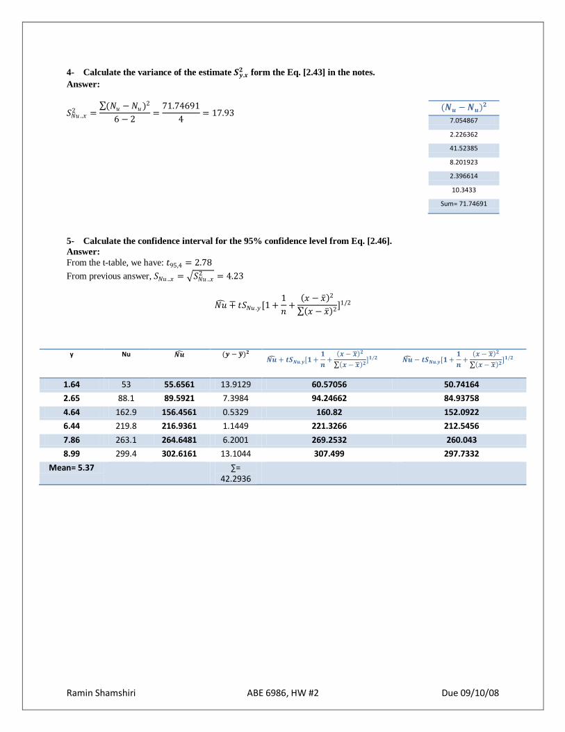
4- Calculate the variance of the estimate 𝑺𝒚.𝒙𝟐 form the Eq. [2.43] in the notes.
Answer:
𝑆𝑁𝑢 ..𝑥2 =
(𝑁𝑢 −𝑁𝑢 )2
6 − 2=71.74691
4= 17.93
(𝑵𝒖 −𝑵𝒖)𝟐
7.054867
2.226362
41.52385
8.201923
2.396614
10.3433
Sum= 71.74691
5- Calculate the confidence interval for the 95% confidence level from Eq. [2.46].
Answer:
From the t-table, we have: 𝑡95,4 = 2.78
From previous answer, 𝑆𝑁𝑢 ..𝑥 = 𝑆𝑁𝑢 ..𝑥2 = 4.23
𝑁𝑢 ∓ 𝑡𝑆𝑁𝑢 .𝑦 [1 +1
𝑛+
𝑥 − 𝑥 2
𝑥 − 𝑥 2]1/2
y Nu 𝑵𝒖 (𝒚 − 𝒚 )𝟐 𝑵𝒖 + 𝒕𝑺𝑵𝒖.𝒚[𝟏+
𝟏
𝒏+
𝒙 − 𝒙 𝟐
𝒙 − 𝒙 𝟐]𝟏/𝟐
𝑵𝒖 − 𝒕𝑺𝑵𝒖.𝒚[𝟏+𝟏
𝒏+
𝒙 − 𝒙 𝟐
𝒙 − 𝒙 𝟐]𝟏/𝟐
1.64 53 55.6561 13.9129 60.57056 50.74164
2.65 88.1 89.5921 7.3984 94.24662 84.93758
4.64 162.9 156.4561 0.5329 160.82 152.0922
6.44 219.8 216.9361 1.1449 221.3266 212.5456
7.86 263.1 264.6481 6.2001 269.2532 260.043
8.99 299.4 302.6161 13.1044 307.499 297.7332
Mean= 5.37 ∑= 42.2936

Ramin Shamshiri ABE 6986, HW #2 Due 09/10/08
6- Plot the confidence band on (1).
Answer:

Ramin Shamshiri ABE 6986, HW #2 Due 09/10/08
7- Discuss your results. How well does the linear model fit the data? What is the physical significance of the
model? What the physical significance of the slope? Would it be appropriate to round off the correlation
coefficient to r=1.00? Why?
Answer:
The linear model has a very high correlation coefficient which shows a very well fit to the data. The linear model shows a good prediction of the response variable, yet it is a simple linear model, easy to plot and analyze. It is not
appropriate to round the correlation coefficient to 1.0 because although the model is a very good one but it is not
perfect. In the other words, r=0.999 does not mean 1.0 and should not be rounded.
Ramin Shamshiri ABE 6986, HW #3 Due 09/17/08
Homework #3
Due 09/17/08
ABE 6986
Ramin Shamshiri
UFID # 90213353
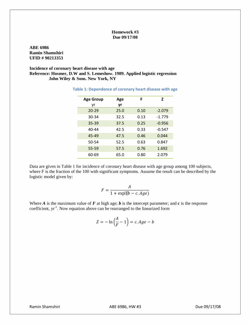
Incidence of coronary heart disease with age
Reference: Hosmer, D.W and S. Lemeshow. 1989. Applied logistic regression
John Wiley & Sons. New York, NY
Table 1: Dependence of coronary heart disease with age
Age Group yr
Age yr
F
Z
20-29 25.0 0.10 -2.079
30-34 32.5 0.13 -1.779
35-39 37.5 0.25 -0.956
40-44 42.5 0.33 -0.547
45-49 47.5 0.46 0.044
50-54 52.5 0.63 0.847
55-59 57.5 0.76 1.692
60-69 65.0 0.80 2.079
Data are given in Table 1 for incidence of coronary heart disease with age group among 100 subjects, where F is the fraction of the 100 with significant symptoms. Assume the result can be described by the
logistic model given by:
𝐹 =𝐴
1 + exp(𝑏 − 𝑐.𝐴𝑔𝑒)
Where A is the maximum value of F at high age; b is the intercept parameter; and c is the response
coefficient, yr-1
. Now equation above can be rearranged to the linearized form
𝑍 = − ln 𝐴
𝐹− 1 = 𝑐.𝐴𝑔𝑒 − 𝑏
Ramin Shamshiri ABE 6986, HW #3 Due 09/17/08
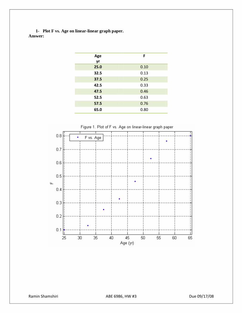
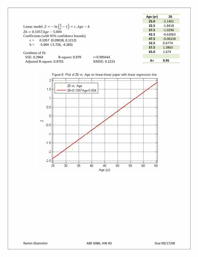
1- Plot F vs. Age on linear-linear graph paper.
Answer:
Age yr
F
25.0 0.10
32.5 0.13
37.5 0.25
42.5 0.33
47.5 0.46
52.5 0.63
57.5 0.76
65.0 0.80
Ramin Shamshiri ABE 6986, HW #3 Due 09/17/08
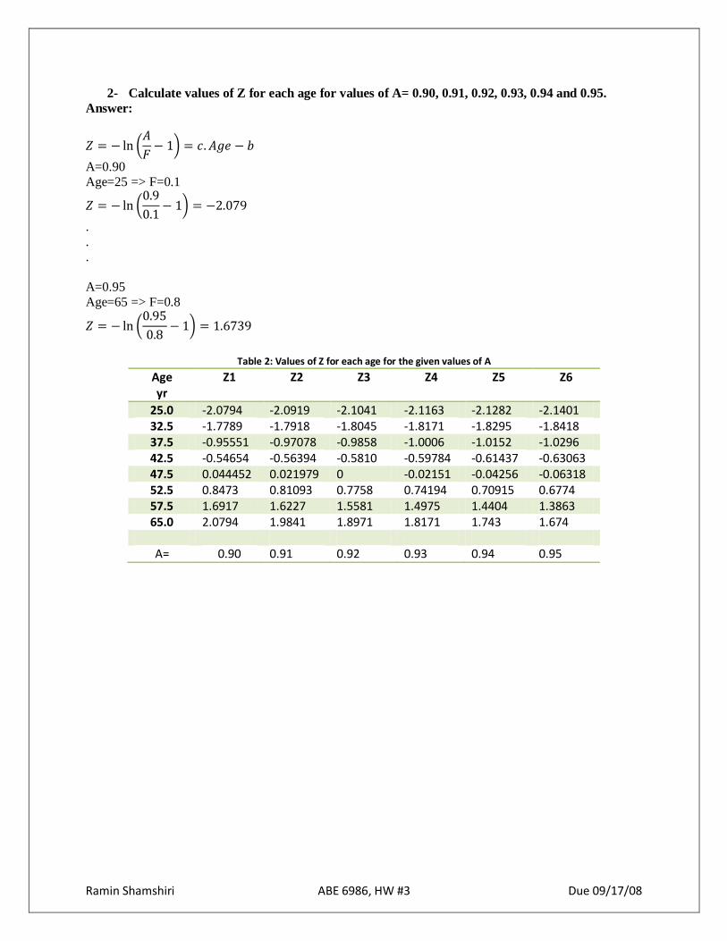
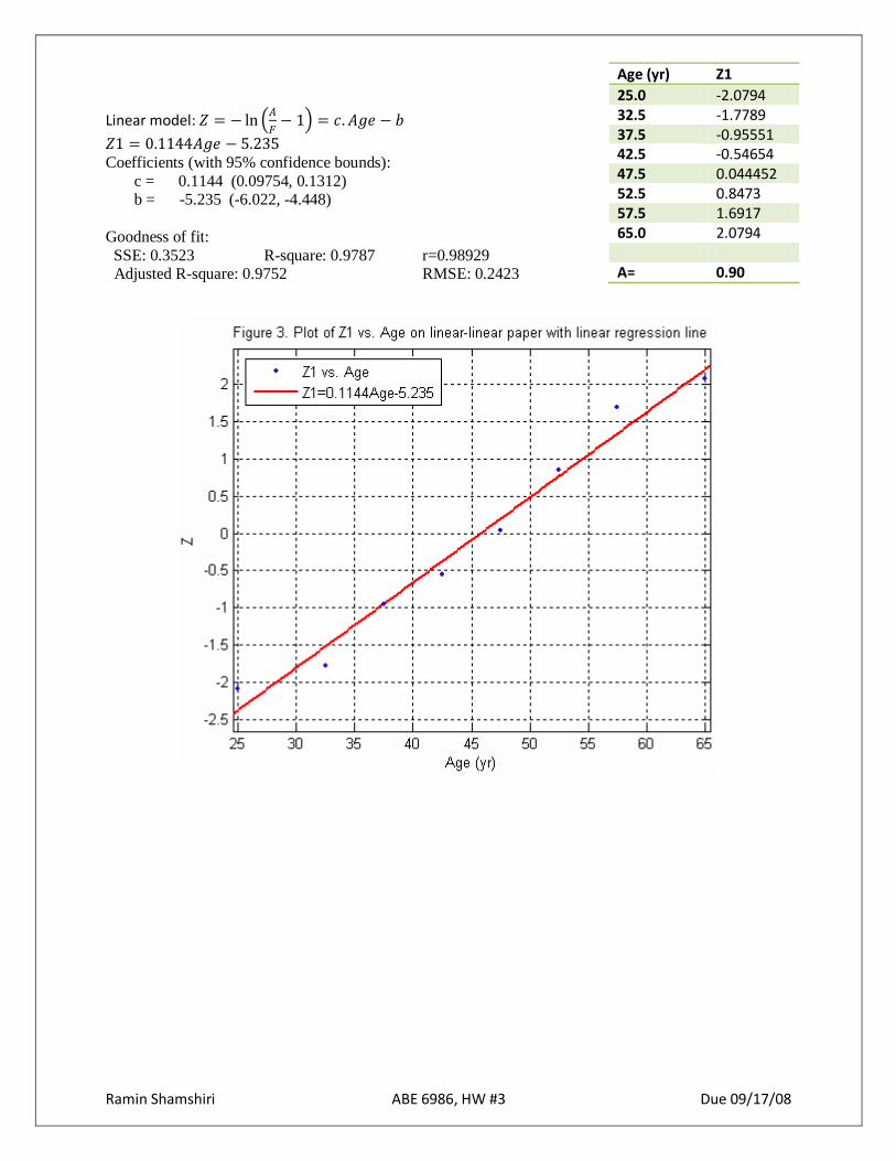
2- Calculate values of Z for each age for values of A= 0.90, 0.91, 0.92, 0.93, 0.94 and 0.95.
Answer:
𝑍 = − ln 𝐴
𝐹− 1 = 𝑐.𝐴𝑔𝑒 − 𝑏
A=0.90
Age=25 => F=0.1
𝑍 = − ln 0.9
0.1− 1 = −2.079
.
.
.
A=0.95
Age=65 => F=0.8
𝑍 = − ln 0.95
0.8− 1 = 1.6739
Table 2: Values of Z for each age for the given values of A
Age yr
Z1
Z2
Z3
Z4 Z5 Z6
25.0 -2.0794 -2.0919 -2.1041 -2.1163 -2.1282 -2.1401 32.5 -1.7789 -1.7918 -1.8045 -1.8171 -1.8295 -1.8418 37.5 -0.95551 -0.97078 -0.9858 -1.0006 -1.0152 -1.0296 42.5 -0.54654 -0.56394 -0.5810 -0.59784 -0.61437 -0.63063 47.5 0.044452 0.021979 0 -0.02151 -0.04256 -0.06318 52.5 0.8473 0.81093 0.7758 0.74194 0.70915 0.6774 57.5 1.6917 1.6227 1.5581 1.4975 1.4404 1.3863 65.0 2.0794 1.9841 1.8971 1.8171 1.743 1.674
A= 0.90 0.91 0.92 0.93 0.94 0.95
Ramin Shamshiri ABE 6986, HW #3 Due 09/17/08
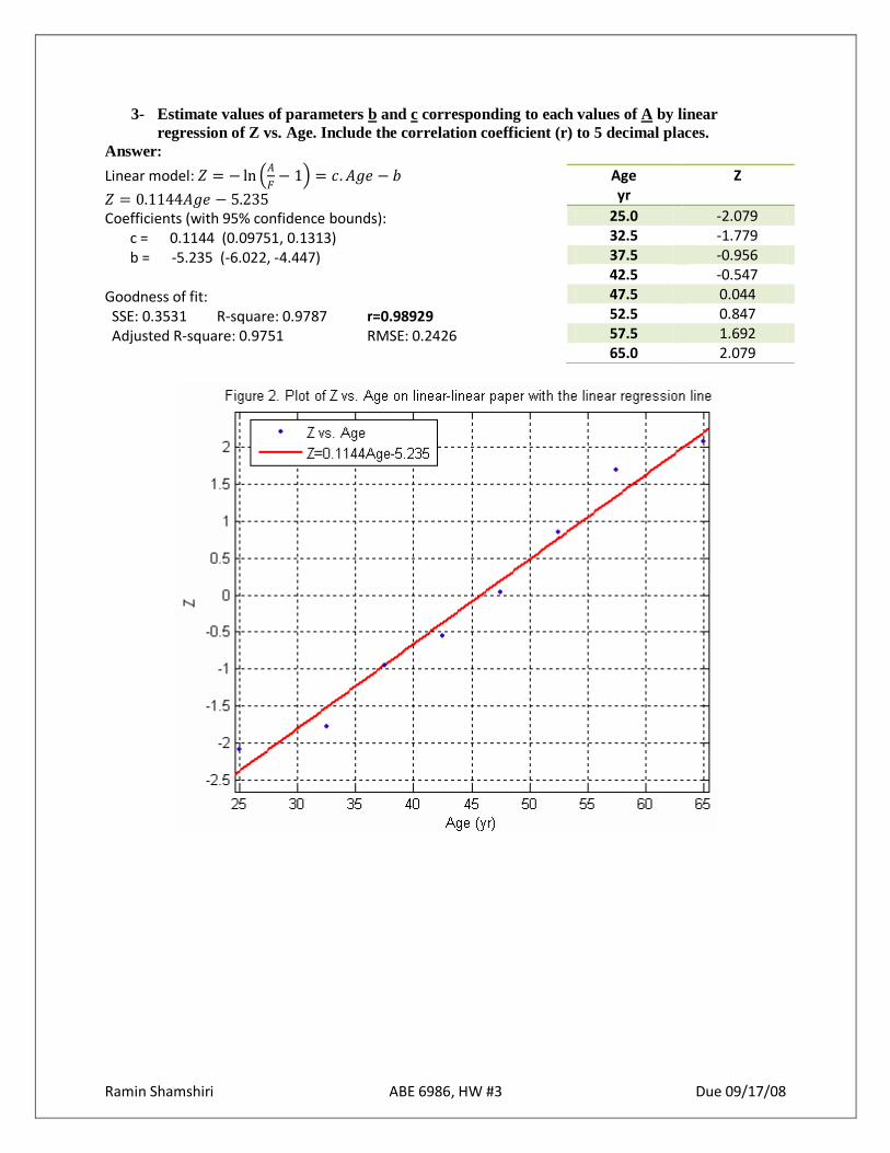
3- Estimate values of parameters b and c corresponding to each values of A by linear
regression of Z vs. Age. Include the correlation coefficient (r) to 5 decimal places.
Answer:
Linear model: 𝑍 = − ln 𝐴
𝐹− 1 = 𝑐.𝐴𝑔𝑒 − 𝑏
𝑍 = 0.1144𝐴𝑔𝑒 − 5.235
Coefficients (with 95% confidence bounds): c = 0.1144 (0.09751, 0.1313) b = -5.235 (-6.022, -4.447) Goodness of fit: SSE: 0.3531 R-square: 0.9787 r=0.98929 Adjusted R-square: 0.9751 RMSE: 0.2426
Age yr
Z
25.0 -2.079 32.5 -1.779 37.5 -0.956 42.5 -0.547 47.5 0.044 52.5 0.847 57.5 1.692 65.0 2.079
Ramin Shamshiri ABE 6986, HW #3 Due 09/17/08
Linear model: 𝑍 = − ln 𝐴
𝐹− 1 = 𝑐.𝐴𝑔𝑒 − 𝑏
𝑍1 = 0.1144𝐴𝑔𝑒 − 5.235
Coefficients (with 95% confidence bounds):
c = 0.1144 (0.09754, 0.1312) b = -5.235 (-6.022, -4.448)
Goodness of fit:
SSE: 0.3523 R-square: 0.9787 r=0.98929 Adjusted R-square: 0.9752 RMSE: 0.2423
Age (yr) Z1
25.0 -2.0794 32.5 -1.7789 37.5 -0.95551 42.5 -0.54654 47.5 0.044452 52.5 0.8473 57.5 1.6917 65.0 2.0794
A= 0.90
Ramin Shamshiri ABE 6986, HW #3 Due 09/17/08
Linear model: 𝑍 = − ln 𝐴
𝐹− 1 = 𝑐.𝐴𝑔𝑒 − 𝑏
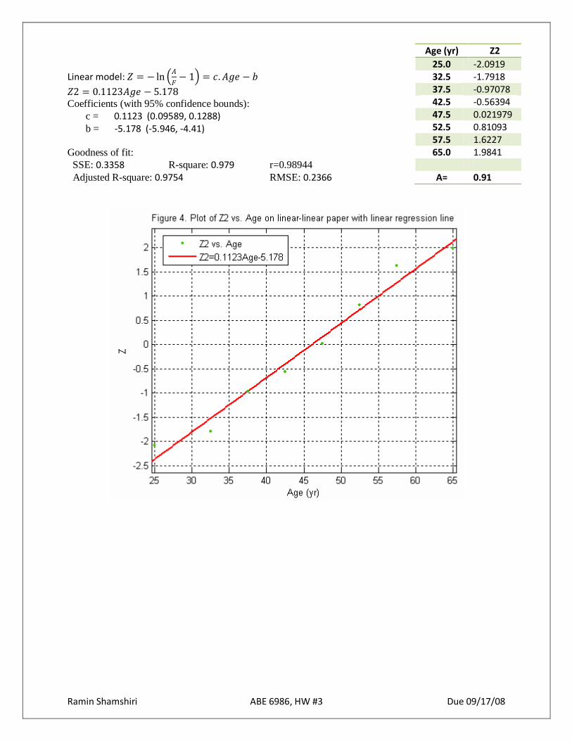
𝑍2 = 0.1123𝐴𝑔𝑒 − 5.178
Coefficients (with 95% confidence bounds):
c = 0.1123 (0.09589, 0.1288) b = -5.178 (-5.946, -4.41) Goodness of fit:
SSE: 0.3358 R-square: 0.979 r=0.98944
Adjusted R-square: 0.9754 RMSE: 0.2366
Age (yr) Z2
25.0 -2.0919 32.5 -1.7918 37.5 -0.97078 42.5 -0.56394 47.5 0.021979 52.5 0.81093 57.5 1.6227 65.0 1.9841
A= 0.91
Ramin Shamshiri ABE 6986, HW #3 Due 09/17/08
Linear model: 𝑍 = − ln 𝐴
𝐹− 1 = 𝑐.𝐴𝑔𝑒 − 𝑏
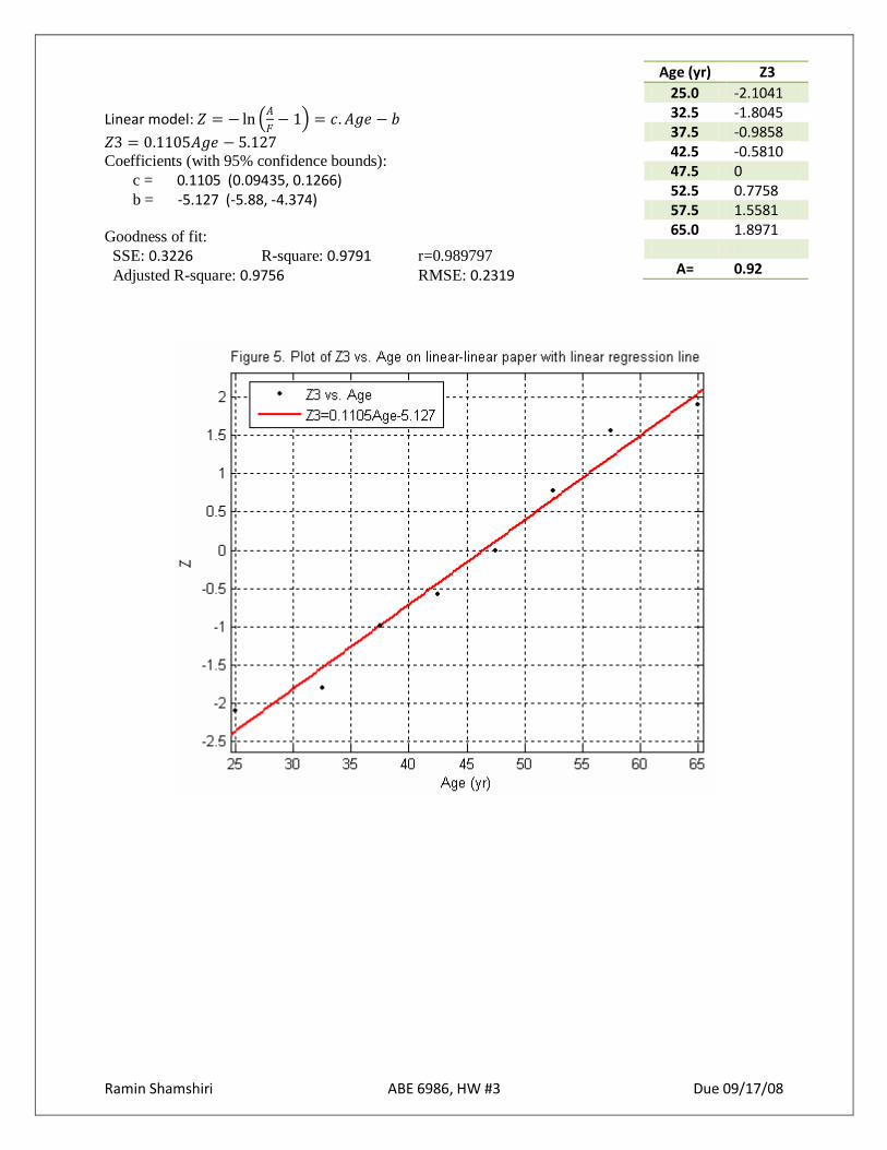
𝑍3 = 0.1105𝐴𝑔𝑒 − 5.127
Coefficients (with 95% confidence bounds):
c = 0.1105 (0.09435, 0.1266) b = -5.127 (-5.88, -4.374) Goodness of fit:
SSE: 0.3226 R-square: 0.9791 r=0.989797
Adjusted R-square: 0.9756 RMSE: 0.2319
Age (yr) Z3
25.0 -2.1041 32.5 -1.8045 37.5 -0.9858 42.5 -0.5810 47.5 0 52.5 0.7758 57.5 1.5581 65.0 1.8971
A= 0.92

Ramin Shamshiri ABE 6986, HW #3 Due 09/17/08
Linear model: 𝑍 = − ln 𝐴
𝐹− 1 = 𝑐.𝐴𝑔𝑒 − 𝑏
𝑍4 = 0.1088𝐴𝑔𝑒 − 5.082
Coefficients (with 95% confidence bounds):
c = 0.1088 (0.09291, 0.1246) b = -5.082 (-5.823, -4.341) Goodness of fit:
SSE: 0.312 R-square: 0.9791 r=0.989494
Adjusted R-square: 0.9757 RMSE: 0.2281
Age (yr) Z4
25.0 -2.1163 32.5 -1.8171 37.5 -1.0006 42.5 -0.59784 47.5 -0.02151 52.5 0.74194 57.5 1.4975 65.0 1.8171
A= 0.93
Ramin Shamshiri ABE 6986, HW #3 Due 09/17/08
Linear model: 𝑍 = − ln 𝐴
𝐹− 1 = 𝑐.𝐴𝑔𝑒 − 𝑏
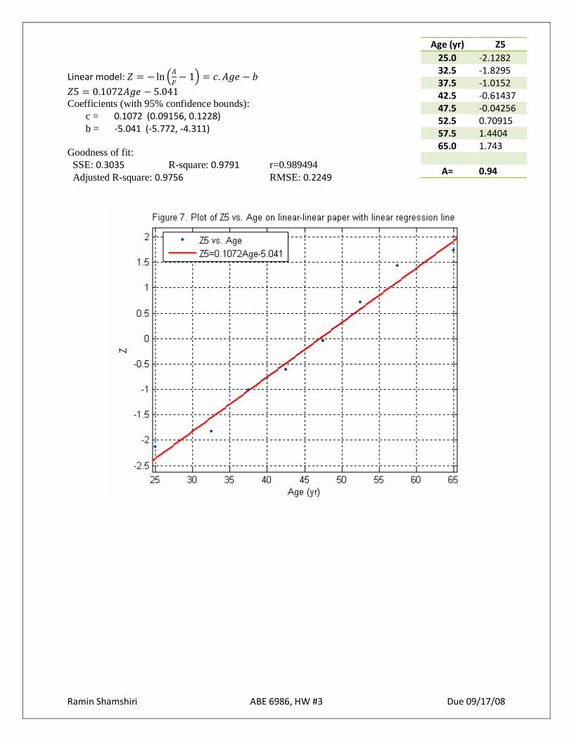
𝑍5 = 0.1072𝐴𝑔𝑒 − 5.041
Coefficients (with 95% confidence bounds):
c = 0.1072 (0.09156, 0.1228) b = -5.041 (-5.772, -4.311) Goodness of fit:
SSE: 0.3035 R-square: 0.9791 r=0.989494
Adjusted R-square: 0.9756 RMSE: 0.2249
Age (yr) Z5
25.0 -2.1282 32.5 -1.8295 37.5 -1.0152 42.5 -0.61437 47.5 -0.04256 52.5 0.70915 57.5 1.4404 65.0 1.743
A= 0.94
Ramin Shamshiri ABE 6986, HW #3 Due 09/17/08
Linear model: 𝑍 = − ln 𝐴
𝐹− 1 = 𝑐.𝐴𝑔𝑒 − 𝑏
𝑍6 = 0.1057𝐴𝑔𝑒 − 5.004
Coefficients (with 95% confidence bounds):
c = 0.1057 (0.09028, 0.1212) b = -5.004 (-5.726, -4.283) Goodness of fit:
SSE: 0.2964 R-square: 0.979 r=0.989444
Adjusted R-square: 0.9755 RMSE: 0.2223
Age (yr) Z6
25.0 -2.1401 32.5 -1.8418 37.5 -1.0296 42.5 -0.63063 47.5 -0.06318 52.5 0.6774 57.5 1.3863 65.0 1.674
A= 0.95
Ramin Shamshiri ABE 6986, HW #3 Due 09/17/08
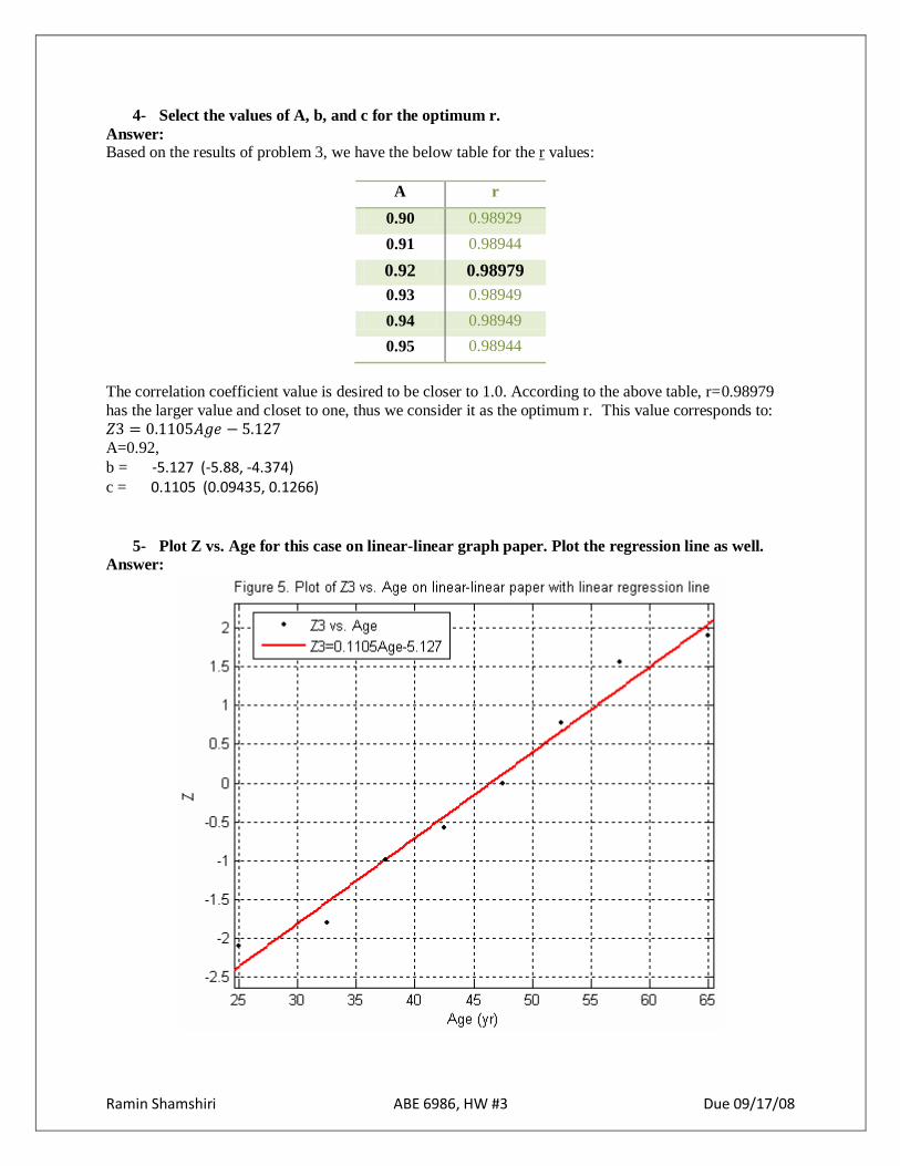
4- Select the values of A, b, and c for the optimum r.
Answer: Based on the results of problem 3, we have the below table for the r values:
A r
0.90 0.98929
0.91 0.98944
0.92 0.98979
0.93 0.98949
0.94 0.98949
0.95 0.98944
The correlation coefficient value is desired to be closer to 1.0. According to the above table, r=0.98979
has the larger value and closet to one, thus we consider it as the optimum r. This value corresponds to:
𝑍3 = 0.1105𝐴𝑔𝑒 − 5.127
A=0.92,
b = -5.127 (-5.88, -4.374) c = 0.1105 (0.09435, 0.1266)
5- Plot Z vs. Age for this case on linear-linear graph paper. Plot the regression line as well.
Answer:
Ramin Shamshiri ABE 6986, HW #3 Due 09/17/08
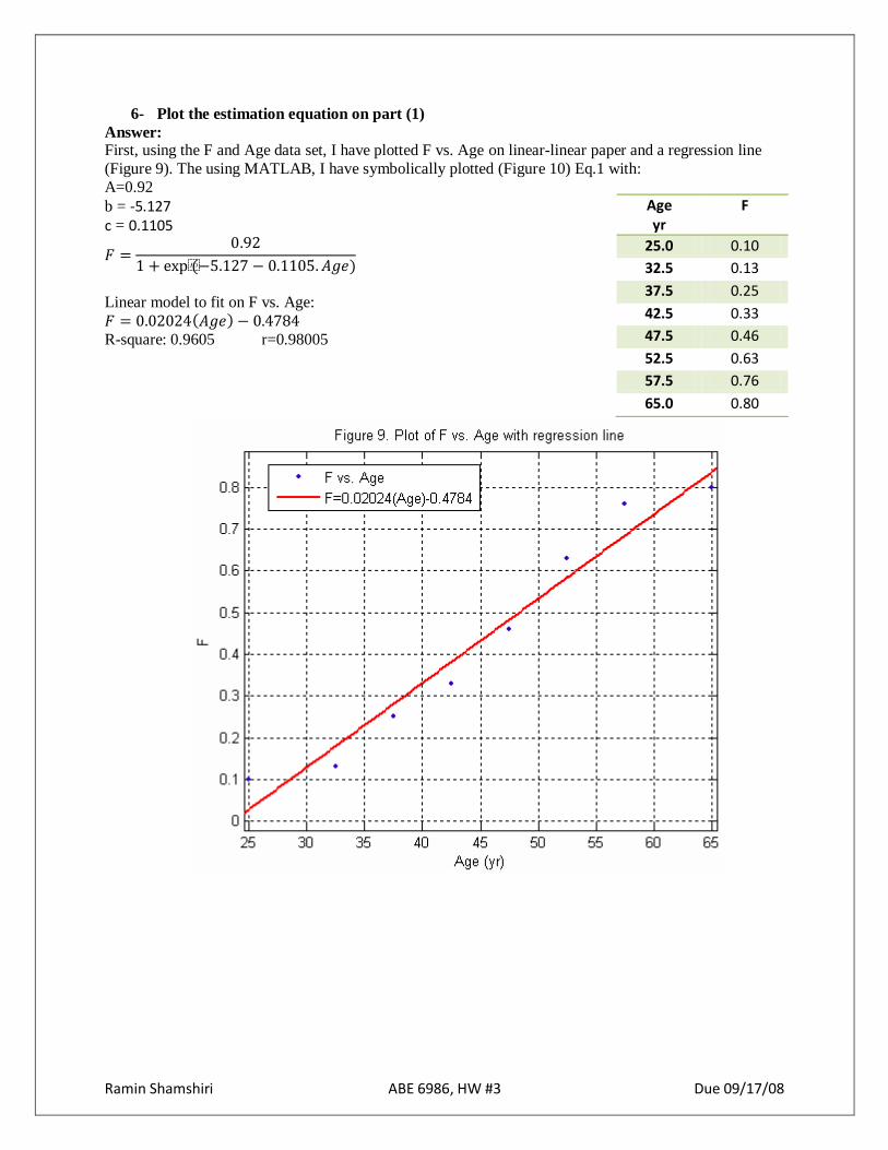
6- Plot the estimation equation on part (1)
Answer: First, using the F and Age data set, I have plotted F vs. Age on linear-linear paper and a regression line
(Figure 9). The using MATLAB, I have symbolically plotted (Figure 10) Eq.1 with:
A=0.92
b = -5.127 c = 0.1105
𝐹 =0.92
1 + exp(−5.127 − 0.1105.𝐴𝑔𝑒)
Linear model to fit on F vs. Age:
𝐹 = 0.02024 𝐴𝑔𝑒 − 0.4784
R-square: 0.9605 r=0.98005
Age yr
F
25.0 0.10
32.5 0.13
37.5 0.25
42.5 0.33
47.5 0.46
52.5 0.63
57.5 0.76
65.0 0.80
Ramin Shamshiri ABE 6986, HW #3 Due 09/17/08
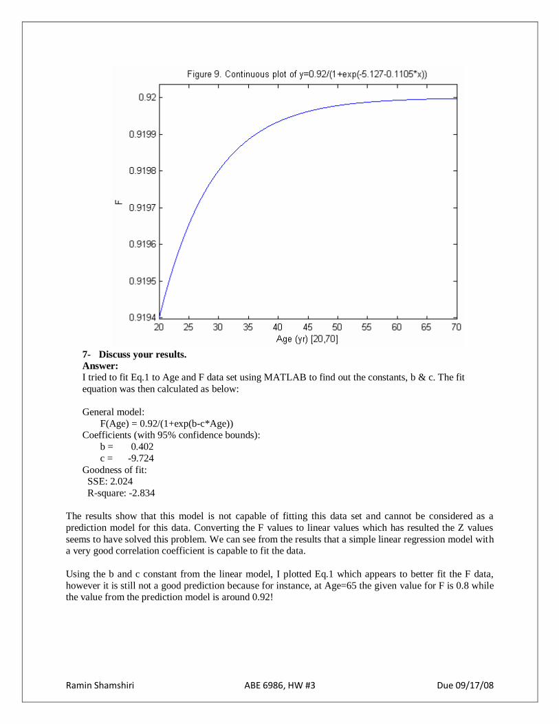
7- Discuss your results.
Answer:
I tried to fit Eq.1 to Age and F data set using MATLAB to find out the constants, b & c. The fit
equation was then calculated as below:
General model:
F(Age) = 0.92/(1+exp(b-c*Age)) Coefficients (with 95% confidence bounds):
b = 0.402
c = -9.724
Goodness of fit: SSE: 2.024
R-square: -2.834
The results show that this model is not capable of fitting this data set and cannot be considered as a
prediction model for this data. Converting the F values to linear values which has resulted the Z values
seems to have solved this problem. We can see from the results that a simple linear regression model with a very good correlation coefficient is capable to fit the data.
Using the b and c constant from the linear model, I plotted Eq.1 which appears to better fit the F data,
however it is still not a good prediction because for instance, at Age=65 the given value for F is 0.8 while the value from the prediction model is around 0.92!
Ramin Shamshiri ABE 6986, HW #4 Due 09/24/08
Homework #4
Due 09/24/08
ABE 6986
Ramin Shamshiri
UFID # 90213353
Population dynamics
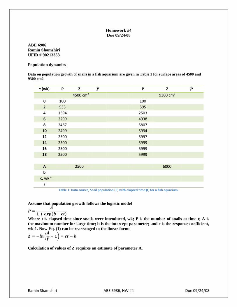
Data on population growth of snails in a fish aquarium are given in Table 1 for surface areas of 4500 and
9300 cm2.
t (wk) P Z 𝑷 P Z 𝑷
4500 cm2 9300 cm2
0 100 100
2 533 595
4 1594 2503
6 2299 4938
8 2467 5807
10 2499 5994
12 2500 5997
14 2500 5999
16 2500 5999
18 2500 5999
A 2500 6000
b
c, wk-1
r
Table 1: Data source, Snail population (P) with elapsed time (t) for a fish aquarium.
Assume that population growth follows the logistic model
𝑷 =𝑨
𝟏 + 𝒆𝒙𝒑 𝒃 − 𝒄𝒕
Where t is elapsed time since snails were introduced, wk; P is the number of snails at time t; A is
the maximum number for large time; b is the intercept parameter; and c is the response coefficient,
wk-1. Now Eq. (1) can be rearranged to the linear form:
𝒁 = −𝒍𝒏 𝑨
𝑷− 𝟏 = 𝒄𝒕 − 𝒃
Calculation of values of Z requires an estimate of parameter A.
Ramin Shamshiri ABE 6986, HW #4 Due 09/24/08
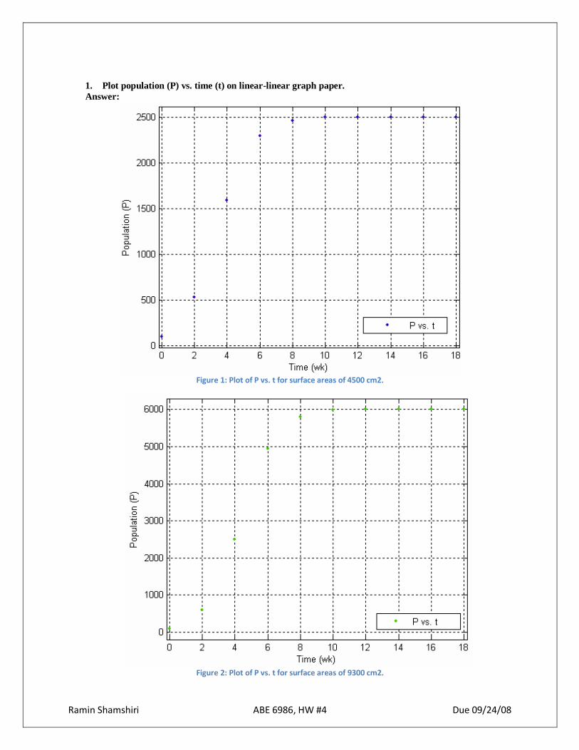
1. Plot population (P) vs. time (t) on linear-linear graph paper.
Answer:
Figure 1: Plot of P vs. t for surface areas of 4500 cm2.
Figure 2: Plot of P vs. t for surface areas of 9300 cm2.
Ramin Shamshiri ABE 6986, HW #4 Due 09/24/08
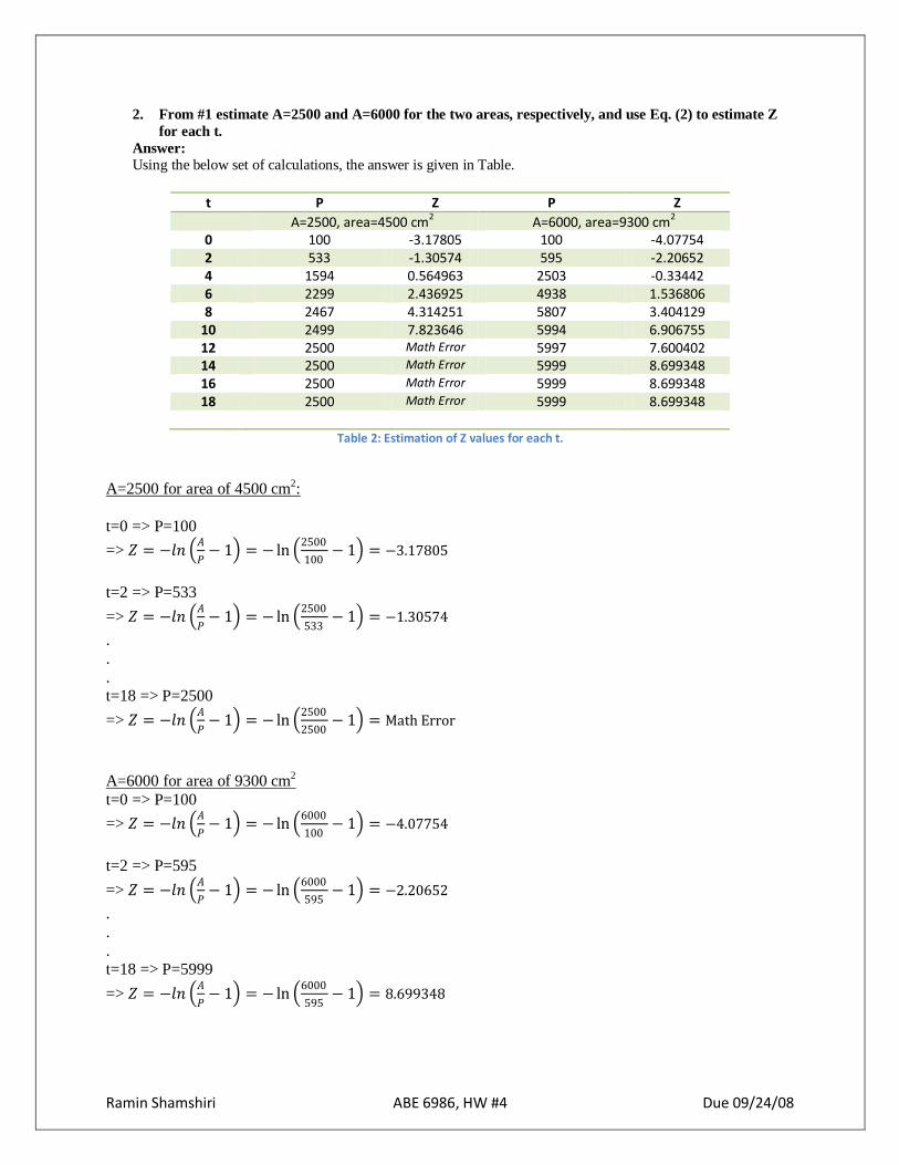
2. From #1 estimate A=2500 and A=6000 for the two areas, respectively, and use Eq. (2) to estimate Z
for each t.
Answer:
Using the below set of calculations, the answer is given in Table.
t P Z P Z
A=2500, area=4500 cm2 A=6000, area=9300 cm2 0 100 -3.17805 100 -4.07754 2 533 -1.30574 595 -2.20652 4 1594 0.564963 2503 -0.33442 6 2299 2.436925 4938 1.536806 8 2467 4.314251 5807 3.404129
10 2499 7.823646 5994 6.906755 12 2500 Math Error 5997 7.600402 14 2500 Math Error 5999 8.699348 16 2500 Math Error 5999 8.699348 18 2500 Math Error 5999 8.699348
Table 2: Estimation of Z values for each t.
A=2500 for area of 4500 cm
2:
t=0 => P=100
=> 𝑍 = −𝑙𝑛 𝐴
𝑃− 1 = − ln
2500
100− 1 = −3.17805
t=2 => P=533
=> 𝑍 = −𝑙𝑛 𝐴
𝑃− 1 = − ln
2500
533− 1 = −1.30574
.
.
. t=18 => P=2500
=> 𝑍 = −𝑙𝑛 𝐴
𝑃− 1 = − ln
2500
2500− 1 = Math Error
A=6000 for area of 9300 cm2
t=0 => P=100
=> 𝑍 = −𝑙𝑛 𝐴
𝑃− 1 = − ln
6000
100− 1 = −4.07754
t=2 => P=595
=> 𝑍 = −𝑙𝑛 𝐴
𝑃− 1 = − ln
6000
595− 1 = −2.20652
.
.
. t=18 => P=5999
=> 𝑍 = −𝑙𝑛 𝐴
𝑃− 1 = − ln
6000
595− 1 = 8.699348
Ramin Shamshiri ABE 6986, HW #4 Due 09/24/08
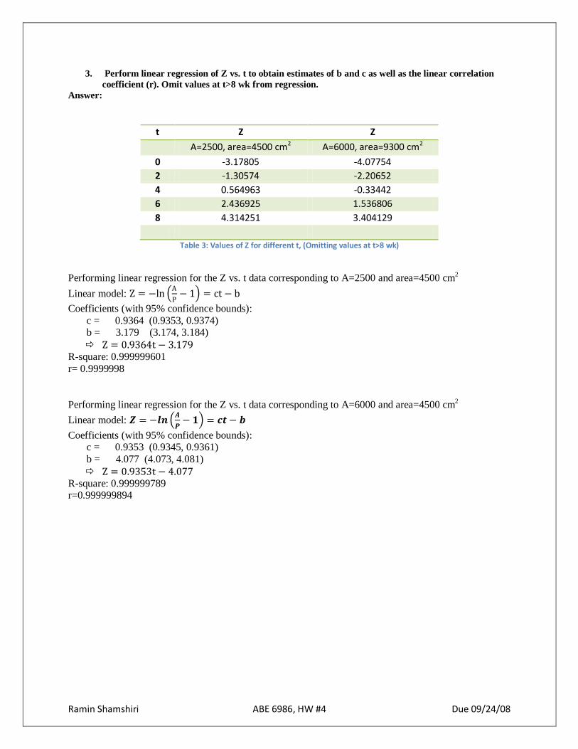
3. Perform linear regression of Z vs. t to obtain estimates of b and c as well as the linear correlation
coefficient (r). Omit values at t>8 wk from regression.
Answer:
t Z Z
A=2500, area=4500 cm2 A=6000, area=9300 cm2
0 -3.17805 -4.07754
2 -1.30574 -2.20652
4 0.564963 -0.33442
6 2.436925 1.536806
8 4.314251 3.404129
Table 3: Values of Z for different t, (Omitting values at t>8 wk)
Performing linear regression for the Z vs. t data corresponding to A=2500 and area=4500 cm2
Linear model: Z = −ln A
P− 1 = ct − b
Coefficients (with 95% confidence bounds):
c = 0.9364 (0.9353, 0.9374) b = 3.179 (3.174, 3.184)
Z = 0.9364t − 3.179 R-square: 0.999999601
r= 0.9999998
Performing linear regression for the Z vs. t data corresponding to A=6000 and area=4500 cm2
Linear model: 𝒁 = −𝒍𝒏 𝑨
𝑷− 𝟏 = 𝒄𝒕 − 𝒃
Coefficients (with 95% confidence bounds): c = 0.9353 (0.9345, 0.9361)
b = 4.077 (4.073, 4.081)
Z = 0.9353t − 4.077 R-square: 0.999999789 r=0.999999894
Ramin Shamshiri ABE 6986, HW #4 Due 09/24/08
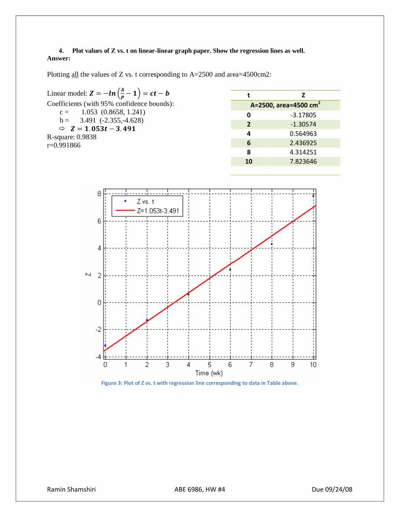
4. Plot values of Z vs. t on linear-linear graph paper. Show the regression lines as well.
Answer:
Plotting all the values of Z vs. t corresponding to A=2500 and area=4500cm2:
Linear model: 𝒁 = −𝒍𝒏 𝑨
𝑷− 𝟏 = 𝒄𝒕 − 𝒃
Coefficients (with 95% confidence bounds):
c = 1.053 (0.8658, 1.241)
b = 3.491 (-2.355,-4.628)
𝒁 = 𝟏.𝟎𝟓𝟑𝒕 − 𝟑.𝟒𝟗𝟏 R-square: 0.9838
r=0.991866
Figure 3: Plot of Z vs. t with regression line corresponding to data in Table above.
t Z
A=2500, area=4500 cm2
0 -3.17805
2 -1.30574
4 0.564963
6 2.436925
8 4.314251
10 7.823646
Ramin Shamshiri ABE 6986, HW #4 Due 09/24/08
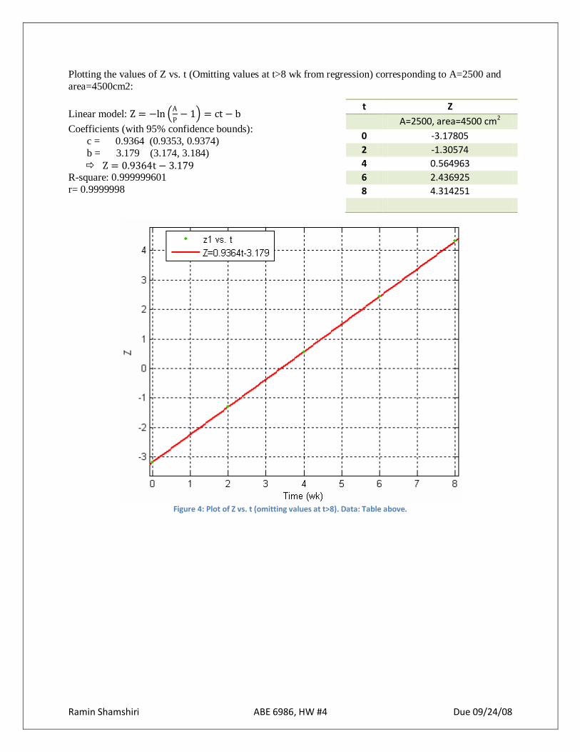
Plotting the values of Z vs. t (Omitting values at t>8 wk from regression) corresponding to A=2500 and
area=4500cm2:
Linear model: Z = −ln A
P− 1 = ct − b
Coefficients (with 95% confidence bounds):
c = 0.9364 (0.9353, 0.9374)
b = 3.179 (3.174, 3.184)
Z = 0.9364t − 3.179 R-square: 0.999999601
r= 0.9999998
Figure 4: Plot of Z vs. t (omitting values at t>8). Data: Table above.
t Z
A=2500, area=4500 cm2
0 -3.17805
2 -1.30574
4 0.564963
6 2.436925
8 4.314251

Ramin Shamshiri ABE 6986, HW #4 Due 09/24/08
Plotting all the values of Z vs. t corresponding to A=6000 and area=9300cm2:
Linear model: Z = −ln A
P− 1 = ct − b
Coefficients (with 95% confidence bounds):
c = 0.7824 (0.6114, 0.9534) b = 3.149 (1.324,4.974)
Z = 0.7824t − 3.149 R-square: 0.933
r=0.96591
Figure 5: Plot of Z vs. t with regression line corresponding to data in Table above.
t Z
A=6000, area=9300 cm2
0 -4.07754 2 -2.20652 4 -0.33442 6 1.536806 8 3.404129
10 6.906755 12 7.600402 14 8.699348 16 8.699348 18 8.699348
Ramin Shamshiri ABE 6986, HW #4 Due 09/24/08
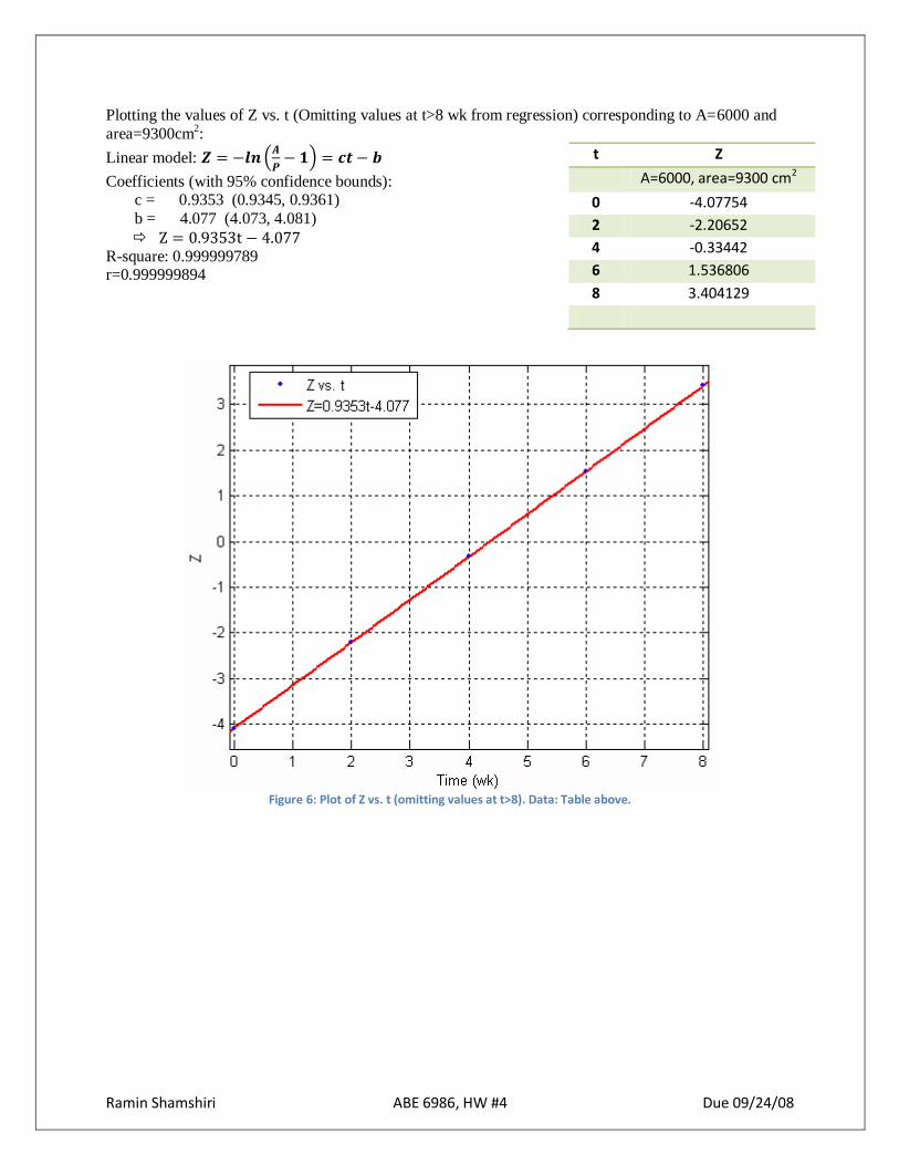
Plotting the values of Z vs. t (Omitting values at t>8 wk from regression) corresponding to A=6000 and
area=9300cm2:
Linear model: 𝒁 = −𝒍𝒏 𝑨
𝑷− 𝟏 = 𝒄𝒕 − 𝒃
Coefficients (with 95% confidence bounds): c = 0.9353 (0.9345, 0.9361)
b = 4.077 (4.073, 4.081)
Z = 0.9353t − 4.077 R-square: 0.999999789 r=0.999999894
Figure 6: Plot of Z vs. t (omitting values at t>8). Data: Table above.
t Z
A=6000, area=9300 cm2
0 -4.07754
2 -2.20652
4 -0.33442
6 1.536806
8 3.404129
Ramin Shamshiri ABE 6986, HW #4 Due 09/24/08
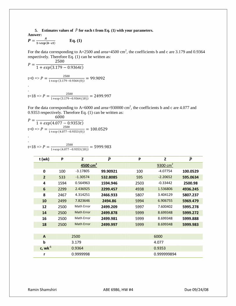
5. Estimates values of 𝑃 for each t from Eq. (1) with your parameters.
Answer:
𝑷 =𝑨
𝟏+𝒆𝒙𝒑 𝒃−𝒄𝒕 Eq. (1)
For the data corresponding to A=2500 and area=4500 cm2, the coefficients b and c are 3.179 and 0.9364
respectively. Therefore Eq. (1) can be written as:
𝑃 =2500
1 + 𝑒𝑥𝑝 3.179 − 0.9364𝑡
t=0 => 𝑃 =2500
1+𝑒𝑥𝑝 3.179−0.9364 (0) = 99.9092
.
.
t=18 => 𝑃 =2500
1+𝑒𝑥𝑝 3.179−0.9364 (18) = 2499.997
For the data corresponding to A=6000 and area=930000 cm2, the coefficients b and c are 4.077 and
0.9353 respectively. Therefore Eq. (1) can be written as:
𝑃 =6000
1 + 𝑒𝑥𝑝 4.077 − 0.9353𝑡
t=0 => 𝑃 =2500
1+𝑒𝑥𝑝 4.077−0.9353 (0) = 100.0529
.
.
t=18 => 𝑃 =2500
1+𝑒𝑥𝑝 4.077−0.9353 (18) = 5999.983
t (wk) P Z 𝑷 P Z 𝑷
4500 cm2 9300 cm2
0 100 -3.17805 99.90921 100 -4.07754 100.0529
2 533 -1.30574 532.8085 595 -2.20652 595.0634
4 1594 0.564963 1594.946 2503 -0.33442 2500.98
6 2299 2.436925 2299.457 4938 1.536806 4936.245
8 2467 4.314251 2466.933 5807 3.404129 5807.237
10 2499 7.823646 2494.86 5994 6.906755 5969.479
12 2500 Math Error 2499.209 5997 7.600402 5995.278
14 2500 Math Error 2499.878 5999 8.699348 5999.272
16 2500 Math Error 2499.981 5999 8.699348 5999.888
18 2500 Math Error 2499.997 5999 8.699348 5999.983
A 2500 6000
b 3.179 4.077
c, wk-1 0.9364 0.9353
r 0.9999998 0.999999894
Ramin Shamshiri ABE 6986, HW #4 Due 09/24/08
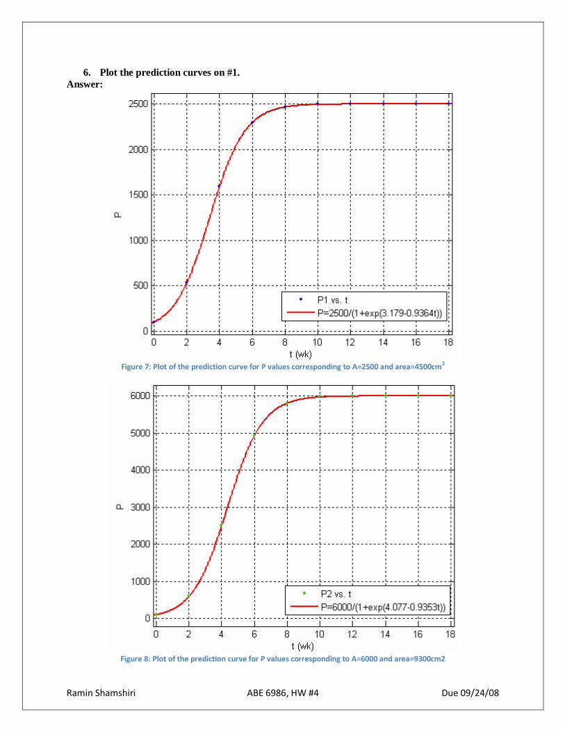
6. Plot the prediction curves on #1.
Answer:
Figure 7: Plot of the prediction curve for P values corresponding to A=2500 and area=4500cm2
Figure 8: Plot of the prediction curve for P values corresponding to A=6000 and area=9300cm2
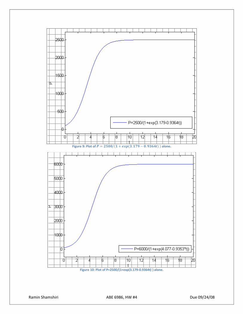
Ramin Shamshiri ABE 6986, HW #4 Due 09/24/08
Figure 9: Plot of 𝑷 = 𝟐𝟓𝟎𝟎/(𝟏 + 𝒆𝒙𝒑(𝟑.𝟏𝟕𝟗− 𝟎.𝟗𝟑𝟔𝟒𝒕) ) alone.
Figure 10: Plot of P=2500/(1+exp(3.179-0.9364t) ) alone.
Ramin Shamshiri ABE 6986, HW #4 Due 09/24/08
7. Discuss your results. How well does the model describe the data? Is the linearization
procedure justified? How could estimates of the parameters be improved? Explain the
effect of surface area on the parameters.
Answer:
The model is a very strong one in predicting the response variable and describing data. Yes, the
linearization procedure is justified because it helped to accurately estimate the b and c coefficients through a simple procedure. This estimation is very accurate as it leaded to a very high correlation
coefficient, very close to 1, however the estimation of the parameters could be improved through non-
linear procedure or with fitting more data.
As the area has increased from 4500 cm2 to 6000 cm2, the values of P have increased too. In the other
word, the surface area has a positive effect on the values of P but a negative effect on the values of Z for
t<10.
Ramin Shamshiri ABE 6986, HW #5 Due 10/08/08
Homework #5
Due 10/08/08
ABE 6986
Ramin Shamshiri
UFID # 90213353
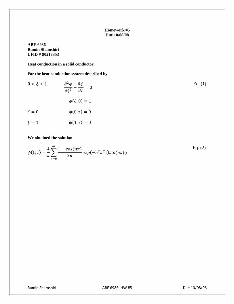
Heat conduction in a solid conductor.
For the heat conduction system described by
0 < 𝜉 < 1 𝜕2𝜙
𝜕𝜉2−
𝜕𝜙
𝜕𝜏= 0
Eq. (1)
𝜙 𝜉, 0 = 1
𝜉 = 0 𝜙 0, 𝜏 = 0
𝜉 = 1 𝜙 1, 𝜏 = 0
We obtained the solution
𝜙 𝜉, 𝜏 =4
𝜋
1 − 𝑐𝑜𝑠(𝑛𝜋)
2𝑛
∞
𝑛=0
𝑒𝑥𝑝 −𝑛2𝜋2𝜏 𝑠𝑖𝑛(𝑛𝜋𝜉) Eq. (2)

Ramin Shamshiri ABE 6986, HW #5 Due 10/08/08
1. Show that Eq. (2) satisfies Eq. (1).
Answer: In order for Equation 2 to satisfy Equation 1, it should be the solution to Eq. (1). In a simply case, if
ax+b=0, then x=-b/a is the answer to this simple equation if substituting (-b/a) with x in the original
equation leads to zero.
Using this argument;
If 𝜉, 𝜏 =4
𝜋
1−𝑐𝑜𝑠 (𝑛𝜋 )
2𝑛
∞𝑛=0 𝑒𝑥𝑝 −𝑛2𝜋2𝜏 𝑠𝑖𝑛(𝑛𝜋𝜉) is the answer to
𝜕2𝜙
𝜕𝜉2 −𝜕𝜙
𝜕𝜏= 0, then:
𝜕𝜙
𝜕𝜉=
4
𝜋
1 − 𝑐𝑜𝑠(𝑛𝜋)
2𝑛
∞
𝑛=1
𝑒𝑥𝑝 −𝑛2𝜋2𝜏 (𝑛𝜋 × (𝑐𝑜𝑠 𝑛𝜋𝜉 ] (1)
𝜕2𝜙
𝜕𝜉2 = −
4
𝜋
1 − 𝑐𝑜𝑠(𝑛𝜋)
2𝑛
∞
𝑛=0
𝑒𝑥𝑝 −𝑛2𝜋2𝜏 (𝑛2𝜋2 × (𝑠𝑖𝑛 𝑛𝜋𝜉 ] (2)
𝜕𝜙
𝜕𝜏= −
4
𝜋
1 − 𝑐𝑜𝑠(𝑛𝜋)
2𝑛
∞
𝑛=0
[ 𝑛2𝜋2 × (𝑒𝑥𝑝 −𝑛2𝜋2𝜏 )]𝑠𝑖𝑛(𝑛𝜋𝜉) (3)
Rearranging (2) & (3) reveals that they are the same thing with different signs which vanish each
other away;
𝜕2𝜙
𝜕𝜉2−
𝜕𝜙
𝜕𝜏= −
4
𝜋 (𝑛2𝜋2)
1 − 𝑐𝑜𝑠(𝑛𝜋)
2𝑛
∞
𝑛=0
𝑒𝑥𝑝 −𝑛2𝜋2𝜏 × (𝑠𝑖𝑛 𝑛𝜋𝜉
+ 4
𝜋 𝑛2𝜋2
1 − 𝑐𝑜𝑠(𝑛𝜋)
2𝑛
∞
𝑛=0
𝑒𝑥𝑝 −𝑛2𝜋2𝜏 × 𝑠𝑖𝑛(𝑛𝜋𝜉) = 0
□
Ramin Shamshiri ABE 6986, HW #5 Due 10/08/08
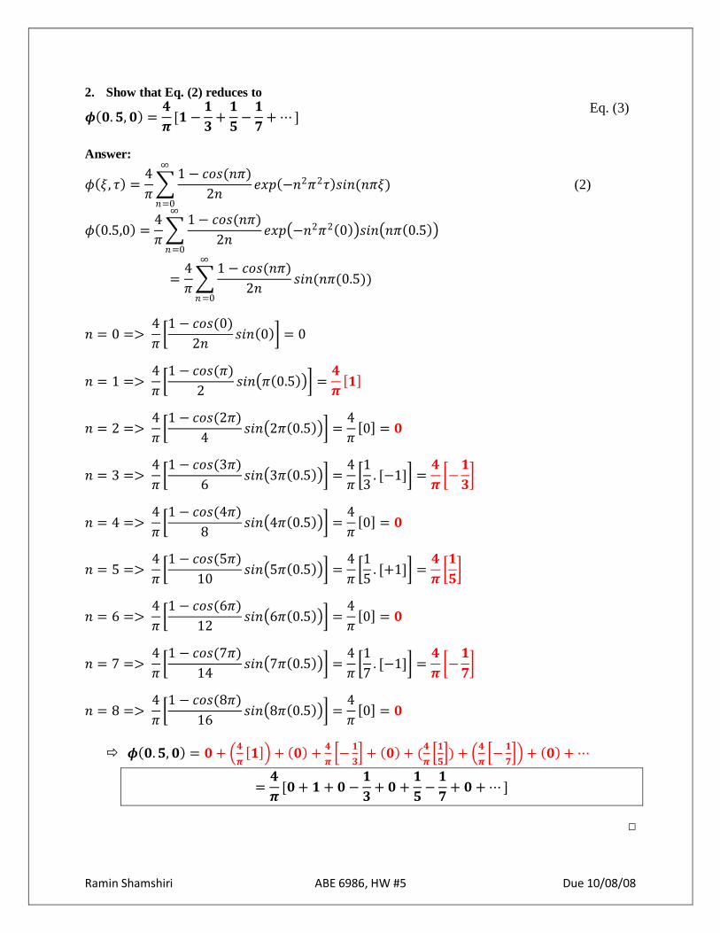
2. Show that Eq. (2) reduces to
𝝓 𝟎. 𝟓, 𝟎 =𝟒
𝝅[𝟏 −
𝟏
𝟑+
𝟏
𝟓−
𝟏
𝟕+ ⋯ ]
Eq. (3)
Answer:
𝜙 𝜉, 𝜏 =4
𝜋
1 − 𝑐𝑜𝑠(𝑛𝜋)
2𝑛
∞
𝑛=0
𝑒𝑥𝑝 −𝑛2𝜋2𝜏 𝑠𝑖𝑛(𝑛𝜋𝜉) (2)
𝜙 0.5,0 =4
𝜋
1 − 𝑐𝑜𝑠(𝑛𝜋)
2𝑛
∞
𝑛=0
𝑒𝑥𝑝 −𝑛2𝜋2 0 𝑠𝑖𝑛 𝑛𝜋 0.5
=4
𝜋
1 − 𝑐𝑜𝑠(𝑛𝜋)
2𝑛
∞
𝑛=0
𝑠𝑖𝑛(𝑛𝜋(0.5))
𝑛 = 0 => 4
𝜋 1 − 𝑐𝑜𝑠(0)
2𝑛𝑠𝑖𝑛 0 = 0
𝑛 = 1 => 4
𝜋 1 − 𝑐𝑜𝑠(𝜋)
2𝑠𝑖𝑛 𝜋 0.5 =
𝟒
𝝅 𝟏
𝑛 = 2 => 4
𝜋 1 − 𝑐𝑜𝑠(2𝜋)
4𝑠𝑖𝑛 2𝜋 0.5 =
4
𝜋 0 = 𝟎
𝑛 = 3 => 4
𝜋 1 − 𝑐𝑜𝑠(3𝜋)
6𝑠𝑖𝑛 3𝜋 0.5 =
4
𝜋 1
3. [−1] =
𝟒
𝝅 −
𝟏
𝟑
𝑛 = 4 => 4
𝜋 1 − 𝑐𝑜𝑠(4𝜋)
8𝑠𝑖𝑛 4𝜋 0.5 =
4
𝜋 0 = 𝟎
𝑛 = 5 => 4
𝜋 1 − 𝑐𝑜𝑠(5𝜋)
10𝑠𝑖𝑛 5𝜋 0.5 =
4
𝜋 1
5. [+1] =
𝟒
𝝅 𝟏
𝟓
𝑛 = 6 => 4
𝜋 1 − 𝑐𝑜𝑠(6𝜋)
12𝑠𝑖𝑛 6𝜋 0.5 =
4
𝜋 0 = 𝟎
𝑛 = 7 => 4
𝜋 1 − 𝑐𝑜𝑠(7𝜋)
14𝑠𝑖𝑛 7𝜋 0.5 =
4
𝜋 1
7. [−1] =
𝟒
𝝅 −
𝟏
𝟕
𝑛 = 8 => 4
𝜋 1 − 𝑐𝑜𝑠(8𝜋)
16𝑠𝑖𝑛 8𝜋 0.5 =
4
𝜋 0 = 𝟎
𝝓 𝟎. 𝟓, 𝟎 = 𝟎 + 𝟒
𝝅 𝟏 + 𝟎 +
𝟒
𝝅 −
𝟏
𝟑 + 𝟎 + (
𝟒
𝝅 𝟏
𝟓 ) +
𝟒
𝝅 −
𝟏
𝟕 + 𝟎 + ⋯
=𝟒
𝝅[𝟎 + 𝟏 + 𝟎 −
𝟏
𝟑+ 𝟎 +
𝟏
𝟓−
𝟏
𝟕+ 𝟎 + ⋯ ]
□
Ramin Shamshiri ABE 6986, HW #5 Due 10/08/08
3. Show by adding terms in Eq. (3) whether it appears to converge to 1.
Answer:
For the first 36 terms, the series becomes equal to 0.9912, therefore, Yes, it appears to converge to
one.
𝝓 𝟎. 𝟓, 𝟎 =𝟒
𝝅 𝟏 −
𝟏
𝟑+
𝟏
𝟓−
𝟏
𝟕+
𝟏
𝟗−
𝟏
𝟏𝟏+
𝟏
𝟏𝟑−
𝟏
𝟏𝟓+
𝟏
𝟏𝟕−
𝟏
𝟏𝟗+
𝟏
𝟐𝟏−
𝟏
𝟐𝟑+
𝟏
𝟐𝟓−
𝟏
𝟐𝟕+
𝟏
𝟐𝟗
−𝟏
𝟑𝟏+
𝟏
𝟑𝟑−
𝟏
𝟑𝟓+
𝟏
𝟑𝟕−
𝟏
𝟑𝟗+
𝟏
𝟒𝟏−
𝟏
𝟒𝟑+
𝟏
𝟒𝟓−
𝟏
𝟒𝟕+
𝟏
𝟒𝟗−
𝟏
𝟓𝟏+
𝟏
𝟓𝟑−
𝟏
𝟓𝟓
+𝟏
𝟓𝟕−
𝟏
𝟓𝟗+
𝟏
𝟔𝟏−
𝟏
𝟔𝟑+
𝟏
𝟔𝟓−
𝟏
𝟔𝟕+
𝟏
𝟔𝟗−
𝟏
𝟕𝟏+ …
= 0.9912 □
4. Discuss the rate of convergence of Eq. (3).
Answer:
The general sequence of the above series can be written as below:
𝝓 𝟎. 𝟓, 𝟎 =𝟒
𝝅 𝟏 −
𝟏
𝟑+
𝟏
𝟓−
𝟏
𝟕+ ⋯ =
𝟒
𝝅 −𝟏 𝒏
𝟐𝒏 + 𝟏
∞
𝒏=𝟎
For the first 6 terms, we will have:
𝟒
𝝅 𝟏 −
𝟏
𝟑+
𝟏
𝟓−
𝟏
𝟕+
𝟏
𝟗−
𝟏
𝟏𝟏 = 𝟎. 𝟗𝟒𝟕𝟑
From the previous results, we found out that after 36 terms, the series value become 0.9912. It can be
seen from this result that the speed at which the above series converges is fast in the first terms but then it
becomes slow. This might be due to the oscillation behavior of the series which was originally resulted
from the positive and negative signs of Sine and Cosine functions that add and subtract terms in order to
converge to 1. This behavior is shown in the general sequence of the series through (-1)n .
□
Ramin Shamshiri ABE 6986, HW #6 Due 10/15/08
Homework #6
Due 10/15/08
ABE 6986
Ramin Shamshiri
UFID # 90213353
Stirred tank chemical reactor
We obtain the solution
𝑪
𝑪𝒔= 𝟏 − 𝐞𝐱𝐩[−
𝑸
𝑽+ 𝒌 𝒕] Eq.1
𝑪𝒔
𝑪𝟎=
𝟏
𝟏 + 𝜶=
𝟏
𝟏 +𝒌𝑽𝑸
Eq.2
Where t is elapsed time, C is the chemical concentration, Cs is steady state concentration, V is
volume of the tank, Q is volumetric flow rate, and k is the 1st order rate constant. Fr a given
experiment assume V=20L and Q=4.0 L h-1
. The reactor was run until steady state conditions of
Cs/C0=0.20 were obtained.
1. Estimate the value of the rate coefficient k.
Answer:
If
V=20L
Q=4.0 L h-1
Cs/C0=0.20 Then
𝐶𝑠
𝐶0=
1
1 +𝑘𝑉𝑄
=> 0.2 =1
1 +204 𝑘
1+5k=5 So k=4/5 or 0.8
Ramin Shamshiri ABE 6986, HW #6 Due 10/15/08
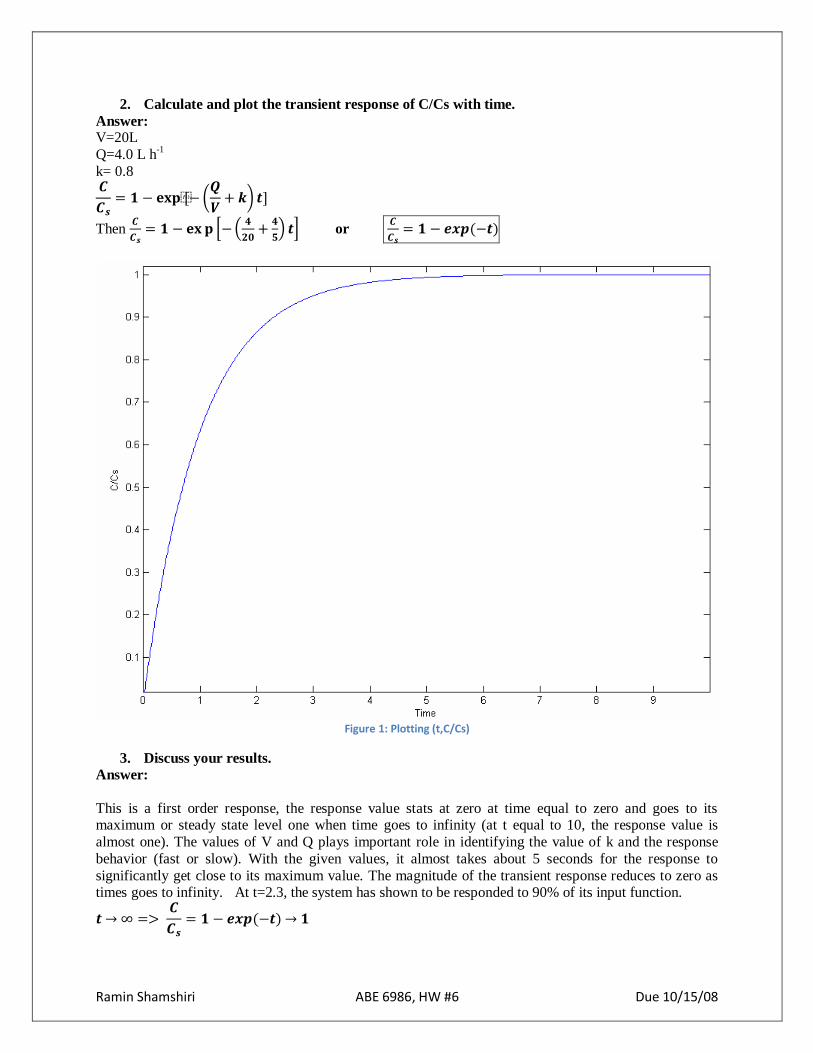
2. Calculate and plot the transient response of C/Cs with time.
Answer: V=20L
Q=4.0 L h-1
k= 0.8 𝑪
𝑪𝒔= 𝟏 − 𝐞𝐱𝐩[−
𝑸
𝑽+ 𝒌 𝒕]
Then 𝑪
𝑪𝒔= 𝟏 − 𝐞𝐱𝐩 −
𝟒
𝟐𝟎+
𝟒
𝟓 𝒕 or
𝑪
𝑪𝒔= 𝟏 − 𝒆𝒙𝒑(−𝒕)
Figure 1: Plotting (t,C/Cs)
3. Discuss your results.
Answer:
This is a first order response, the response value stats at zero at time equal to zero and goes to its maximum or steady state level one when time goes to infinity (at t equal to 10, the response value is
almost one). The values of V and Q plays important role in identifying the value of k and the response
behavior (fast or slow). With the given values, it almost takes about 5 seconds for the response to
significantly get close to its maximum value. The magnitude of the transient response reduces to zero as times goes to infinity. At t=2.3, the system has shown to be responded to 90% of its input function.
𝒕 ∞ => 𝑪
𝑪𝒔= 𝟏 − 𝒆𝒙𝒑(−𝒕) 𝟏
Ramin Shamshiri ABE 6986, HW #7 Due 10/22/08
Homework #7
Due 10/22/08
Phosphorous transport in a packed bed reactor
The steady state distribution of phosphorus concentration with depth is assumed to follow
𝐂𝐬
𝐂𝟎≅ 𝐞𝐱𝐩(−
𝐤
𝐯𝐳)
(1)
Results are shown in Figure 3 for the four velocities of 0.118, 0.256, 0.539 and 0.900 cm min-1.
1. Estimate the slope k/v from figure 3 for each velocity.
Answer:
According to Figure 3,
𝑆𝑙𝑜𝑝𝑒 = 𝑡𝑔 𝛼 =Δ𝑦
Δ𝑥
v=0.118(cm/min)
𝑧 = 2𝑐𝑚 => − ln 𝐶𝑠
𝐶0 = 0.075
𝑧 = 10𝑐𝑚 => − ln 𝐶𝑠
𝐶0 = 0.39
𝑡𝑔 𝛼 =Δ𝑦
Δ𝑥=
0.39 − 0.075
10 − 2= 0.039375
v=0.256(cm/min)
𝑧 = 2𝑐𝑚 => − ln 𝐶𝑠
𝐶0 = 0.05
𝑧 = 10𝑐𝑚 => − ln 𝐶𝑠
𝐶0 = 0.23
𝑡𝑔 𝛼 =Δ𝑦
Δ𝑥=
0.23 − 0.05
10 − 2= 0.0225
v=0.539(cm/min)
𝑧 = 2𝑐𝑚 => − ln 𝐶𝑠
𝐶0 = 0.14
𝑧 = 10𝑐𝑚 => − ln 𝐶𝑠
𝐶0 = 0.02
𝑡𝑔 𝛼 =Δ𝑦
Δ𝑥=
0.14 − 0.02
10 − 2= 0.015
v=0.900(cm/min)
𝑧 = 2𝑐𝑚 => − ln 𝐶𝑠
𝐶0 = 0.02
𝑧 = 10𝑐𝑚 => − ln 𝐶𝑠
𝐶0 = 0.1
𝑡𝑔 𝛼 =Δ𝑦
Δ𝑥=
0.1 − 0.02
10 − 2= 0.01
Ramin Shamshiri ABE 6986, HW #7 Due 10/22/08
2. From (1) estimate the value of k for each velocity.
Answer: 𝐂𝐬
𝐂𝟎≅ 𝐞𝐱𝐩(−
𝐤
𝐯𝐳)
v=0.118 (cm/min)
𝑧 = 10𝑐𝑚 => − ln 𝐶𝑠
𝐶0 = 0.39
−ln Cs
C0 ≅
k
vz ==> 0.39 ≅
k
0.118 cmmin
10 cm
==> 𝑘 =0.39 × 0.118
cmmin
10 cm = 0.004602 (1/min)
v=0.256 (cm/min)
𝑧 = 10𝑐𝑚 => − ln 𝐶𝑠
𝐶0 = 0.23
−ln Cs
C0 ≅
k
vz ==> 0.23 ≅
k
0.256 cmmin
10 cm
==> 𝑘 =0.23 × 0.256
cmmin
10 cm = 0.005888 (1/min)
v=0.539 (cm/min)
𝑧 = 2𝑐𝑚 => − ln 𝐶𝑠
𝐶0 = 0.14
−ln Cs
C0 ≅
k
vz ==> 0.14 ≅
k
0.539 cmmin
10 cm
==> 𝑘 =0.14 × 0.539
cmmin
10 cm = 0.007546 (1/min)
v=0.900 (cm/min)
𝑧 = 10𝑐𝑚 => − ln 𝐶𝑠
𝐶0 = 0.1
−ln Cs
C0 ≅
k
vz ==> 0.1 ≅
k
0.900 cmmin
10 cm
==> 𝑘 =0.1 × 0.900
cmmin
10 cm = 0.009 (1/min)
Ramin Shamshiri ABE 6986, HW #7 Due 10/22/08
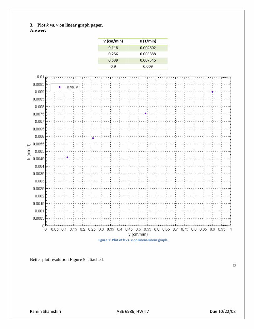
3. Plot k vs. v on linear graph paper.
Answer:
V (cm/min) K (1/min)
0.118 0.004602
0.256 0.005888
0.539 0.007546
0.9 0.009
Figure 1: Plot of k vs. v on linear-linear graph.
Better plot resolution Figure 5 attached.
□
Ramin Shamshiri ABE 6986, HW #7 Due 10/22/08
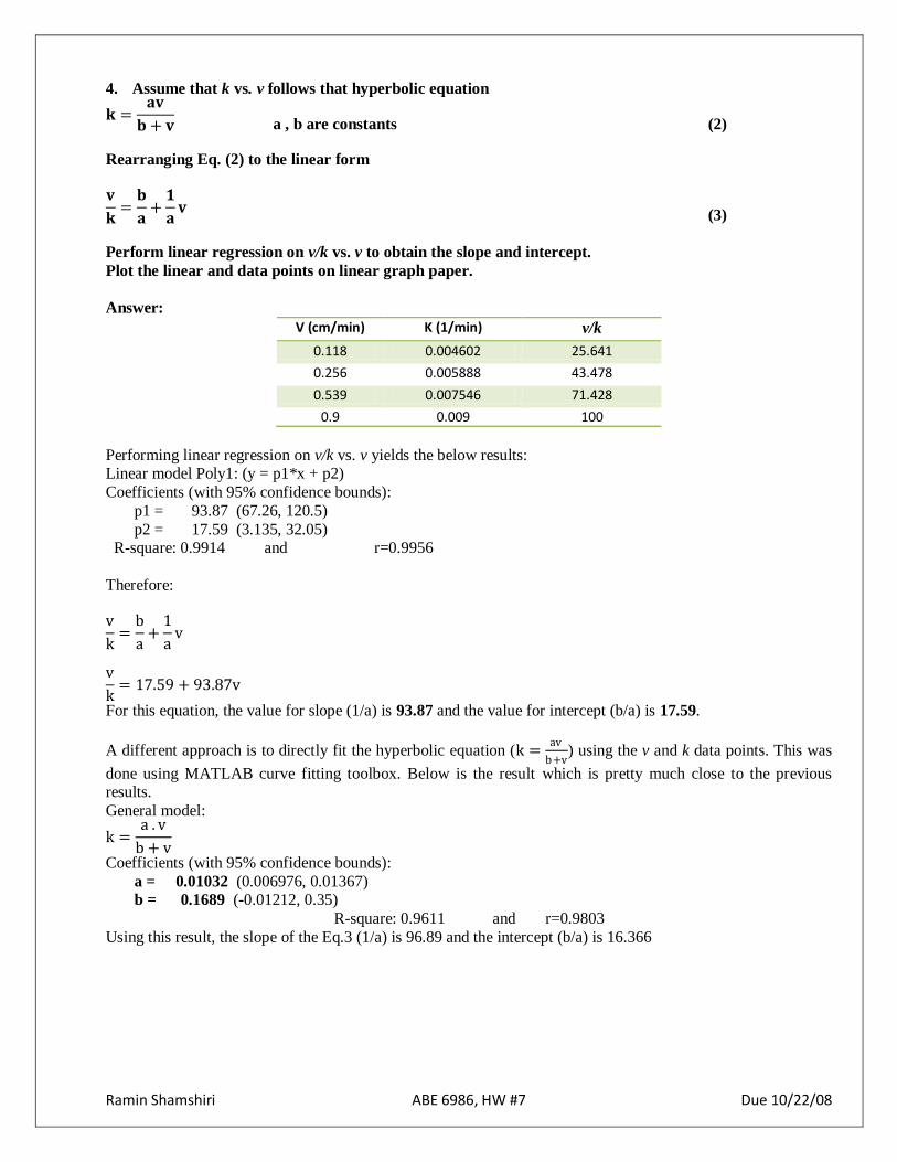
4. Assume that k vs. v follows that hyperbolic equation
𝐤 =𝐚𝐯
𝐛 + 𝐯
a , b are constants (2)
Rearranging Eq. (2) to the linear form
𝐯
𝐤=
𝐛
𝐚+
𝟏
𝐚𝐯
(3)
Perform linear regression on v/k vs. v to obtain the slope and intercept.
Plot the linear and data points on linear graph paper.
Answer:
V (cm/min) K (1/min) v/k
0.118 0.004602 25.641
0.256 0.005888 43.478
0.539 0.007546 71.428
0.9 0.009 100
Performing linear regression on v/k vs. v yields the below results: Linear model Poly1: (y = p1*x + p2)
Coefficients (with 95% confidence bounds):
p1 = 93.87 (67.26, 120.5)
p2 = 17.59 (3.135, 32.05) R-square: 0.9914 and r=0.9956
Therefore: v
k=
b
a+
1
av
v
k= 17.59 + 93.87v
For this equation, the value for slope (1/a) is 93.87 and the value for intercept (b/a) is 17.59.
A different approach is to directly fit the hyperbolic equation (k =av
b+v) using the v and k data points. This was
done using MATLAB curve fitting toolbox. Below is the result which is pretty much close to the previous results.
General model:
k =a . v
b + v
Coefficients (with 95% confidence bounds):
a = 0.01032 (0.006976, 0.01367) b = 0.1689 (-0.01212, 0.35)
R-square: 0.9611 and r=0.9803
Using this result, the slope of the Eq.3 (1/a) is 96.89 and the intercept (b/a) is 16.366
Ramin Shamshiri ABE 6986, HW #7 Due 10/22/08
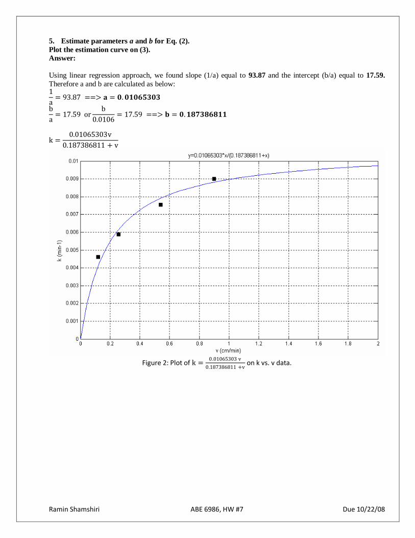
5. Estimate parameters a and b for Eq. (2).
Plot the estimation curve on (3).
Answer:
Using linear regression approach, we found slope (1/a) equal to 93.87 and the intercept (b/a) equal to 17.59.
Therefore a and b are calculated as below: 1
a= 93.87 ==> 𝐚 = 𝟎. 𝟎𝟏𝟎𝟔𝟓𝟑𝟎𝟑
b
a= 17.59 or
b
0.0106= 17.59 ==> 𝐛 = 𝟎.𝟏𝟖𝟕𝟑𝟖𝟔𝟖𝟏𝟏
k =0.01065303v
0.187386811 + v
Figure 2: Plot of k =
0.01065303 v
0.187386811 +v on k vs. v data.
Ramin Shamshiri ABE 6986, HW #7 Due 10/22/08
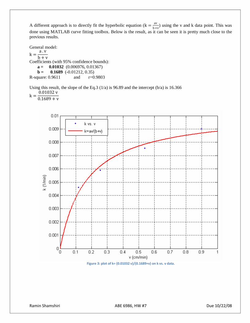
A different approach is to directly fit the hyperbolic equation (k =av
b+v) using the v and k data point. This was
done using MATLAB curve fitting toolbox. Below is the result, as it can be seen it is pretty much close to the previous results.
General model:
k =a . v
b + v
Coefficients (with 95% confidence bounds):
a = 0.01032 (0.006976, 0.01367)
b = 0.1689 (-0.01212, 0.35)
R-square: 0.9611 and r=0.9803
Using this result, the slope of the Eq.3 (1/a) is 96.89 and the intercept (b/a) is 16.366
k =0.01032 v
0.1689 + v
Figure 3: plot of k= (0.01032 v)/(0.1689+v) on k vs. v data.

Ramin Shamshiri ABE 6986, HW #7 Due 10/22/08
6. Discuss your results. What is the upper limit on k?
Does k vs. v approach a straight line as 𝒗 𝟎 ?
Write an equation for characteristic depth, z, for Eq. (1). What does this mean?
Answer:
The upper limit on k from the data points is 0.009 and from the curve equation is almost 0.01 (min-1
). Yes, according to Figure 4, it can be seen that as v get larger and larger, the k vs. v converges to a straight line.
Cs
C0≅ exp(−
k
vz)
ln Cs
C0 = −
k
vz
z = −v
kln(
Cs
C0)
Dimension analysis:
[cm] = −
cmmin
1
min
[1]
It means that the parameter depth depends on the velocity and the absorption rate. The dimension of depth is
also shown to agree with what we can see from the equation.
Figure 4
Ramin Shamshiri ABE 6986, HW #8 Due 10/29/08
Homework #8
Due 10/29/08
Kinetic coefficients for phosphorus transport in a packed bed reactor
Refernce: Overman, A.R., Data points for Figure 7 of the article are given in Table 1 below.
v
(cm/min) Ka
(min-1) Kd
(min-1) Kr
(min-1)
0.118 1.10 0.0314 0.00013
0.256 2.00 0.0790 0.00024
0.539 2.75 0.133 0.00035
0.900 3.00 0.155 0.00047
Table 1: Dependence of coefficients for adsorption (Ka), desorption (Kd), and reaction (Kr) on flow velocity (v)
for phosphorus transport in a packed bed reactor.
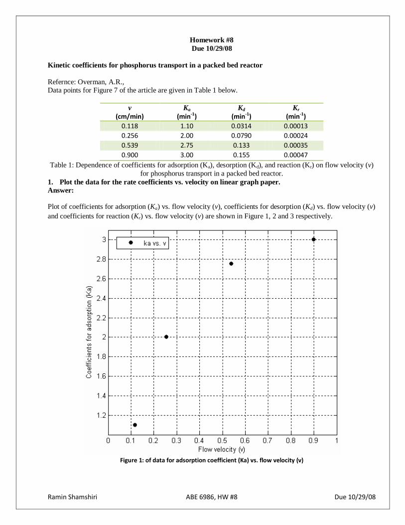
1. Plot the data for the rate coefficients vs. velocity on linear graph paper.
Answer:
Plot of coefficients for adsorption (Ka) vs. flow velocity (v), coefficients for desorption (Kd) vs. flow velocity (v)
and coefficients for reaction (Kr) vs. flow velocity (v) are shown in Figure 1, 2 and 3 respectively.
Figure 1: of data for adsorption coefficient (Ka) vs. flow velocity (v)
Ramin Shamshiri ABE 6986, HW #8 Due 10/29/08
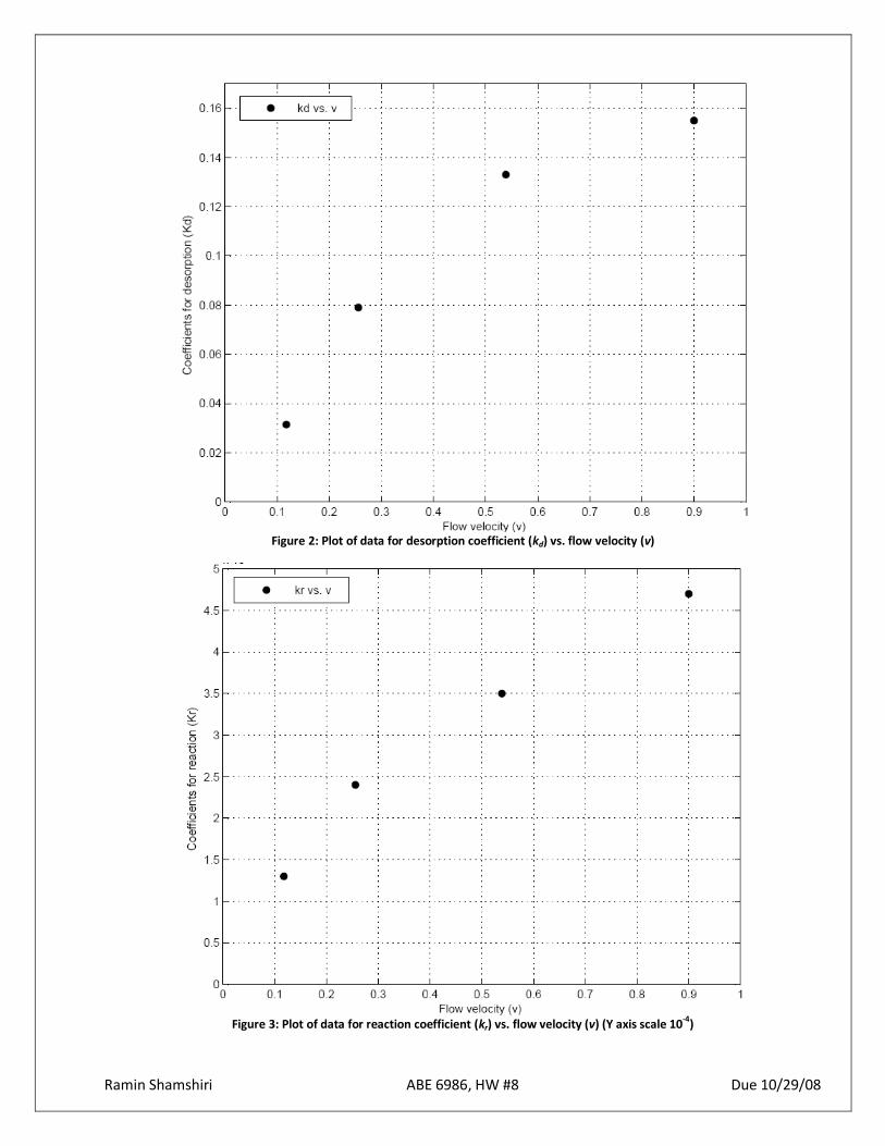
Figure 2: Plot of data for desorption coefficient (kd) vs. flow velocity (v)
Figure 3: Plot of data for reaction coefficient (kr) vs. flow velocity (v) (Y axis scale 10-4)
Ramin Shamshiri ABE 6986, HW #8 Due 10/29/08
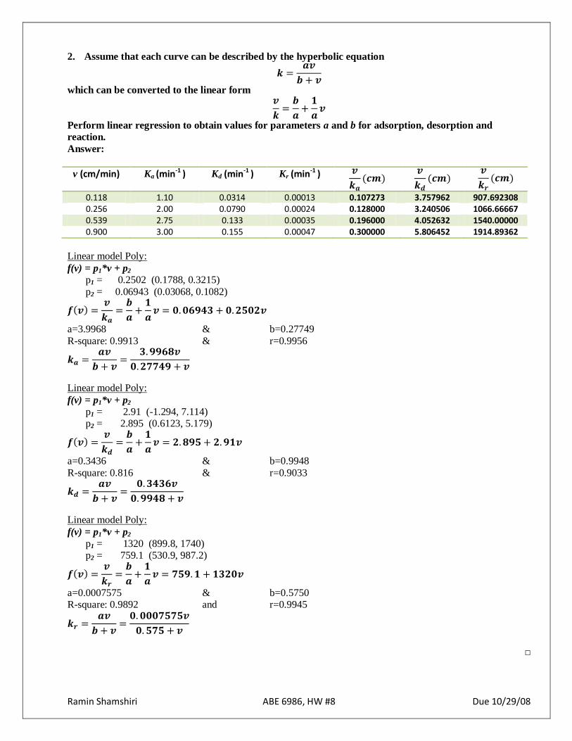
2. Assume that each curve can be described by the hyperbolic equation
𝒌 =𝒂𝒗
𝒃 + 𝒗
which can be converted to the linear form 𝒗
𝒌=
𝒃
𝒂+
𝟏
𝒂𝒗
Perform linear regression to obtain values for parameters a and b for adsorption, desorption and
reaction.
Answer:
v (cm/min) Ka (min-1 ) Kd (min-1 ) Kr (min-1 ) 𝒗
𝒌𝒂(𝒄𝒎)
𝒗
𝒌𝒅(𝒄𝒎)
𝒗
𝒌𝒓(𝒄𝒎)
0.118 1.10 0.0314 0.00013 0.107273 3.757962 907.692308 0.256 2.00 0.0790 0.00024 0.128000 3.240506 1066.66667 0.539 2.75 0.133 0.00035 0.196000 4.052632 1540.00000 0.900 3.00 0.155 0.00047 0.300000 5.806452 1914.89362
Linear model Poly:
f(v) = p1*v + p2
p1 = 0.2502 (0.1788, 0.3215)
p2 = 0.06943 (0.03068, 0.1082)
𝒇 𝒗 =𝒗
𝒌𝒂=
𝒃
𝒂+
𝟏
𝒂𝒗 = 𝟎.𝟎𝟔𝟗𝟒𝟑 + 𝟎.𝟐𝟓𝟎𝟐𝒗
a=3.9968 & b=0.27749
R-square: 0.9913 & r=0.9956
𝒌𝒂 =𝒂𝒗
𝒃 + 𝒗=
𝟑.𝟗𝟗𝟔𝟖𝒗
𝟎.𝟐𝟕𝟕𝟒𝟗 + 𝒗
Linear model Poly:
f(v) = p1*v + p2
p1 = 2.91 (-1.294, 7.114) p2 = 2.895 (0.6123, 5.179)
𝒇 𝒗 =𝒗
𝒌𝒅=
𝒃
𝒂+
𝟏
𝒂𝒗 = 𝟐.𝟖𝟗𝟓 + 𝟐.𝟗𝟏𝒗
a=0.3436 & b=0.9948
R-square: 0.816 & r=0.9033
𝒌𝒅 =𝒂𝒗
𝒃 + 𝒗=
𝟎.𝟑𝟒𝟑𝟔𝒗
𝟎.𝟗𝟗𝟒𝟖 + 𝒗
Linear model Poly:
f(v) = p1*v + p2
p1 = 1320 (899.8, 1740) p2 = 759.1 (530.9, 987.2)
𝒇 𝒗 =𝒗
𝒌𝒓=
𝒃
𝒂+
𝟏
𝒂𝒗 = 𝟕𝟓𝟗.𝟏 + 𝟏𝟑𝟐𝟎𝒗
a=0.0007575 & b=0.5750 R-square: 0.9892 and r=0.9945
𝒌𝒓 =𝒂𝒗
𝒃 + 𝒗=
𝟎. 𝟎𝟎𝟎𝟕𝟓𝟕𝟓𝒗
𝟎. 𝟓𝟕𝟓 + 𝒗
□
Ramin Shamshiri ABE 6986, HW #8 Due 10/29/08
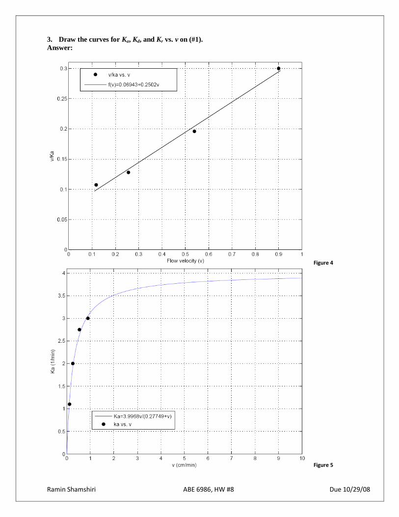
3. Draw the curves for Ka, Kd, and Kr vs. v on (#1).
Answer:
Figure 4
Figure 5
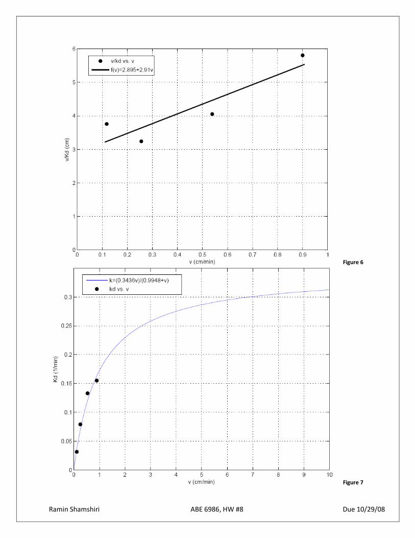
Ramin Shamshiri ABE 6986, HW #8 Due 10/29/08
Figure 6
Figure 7
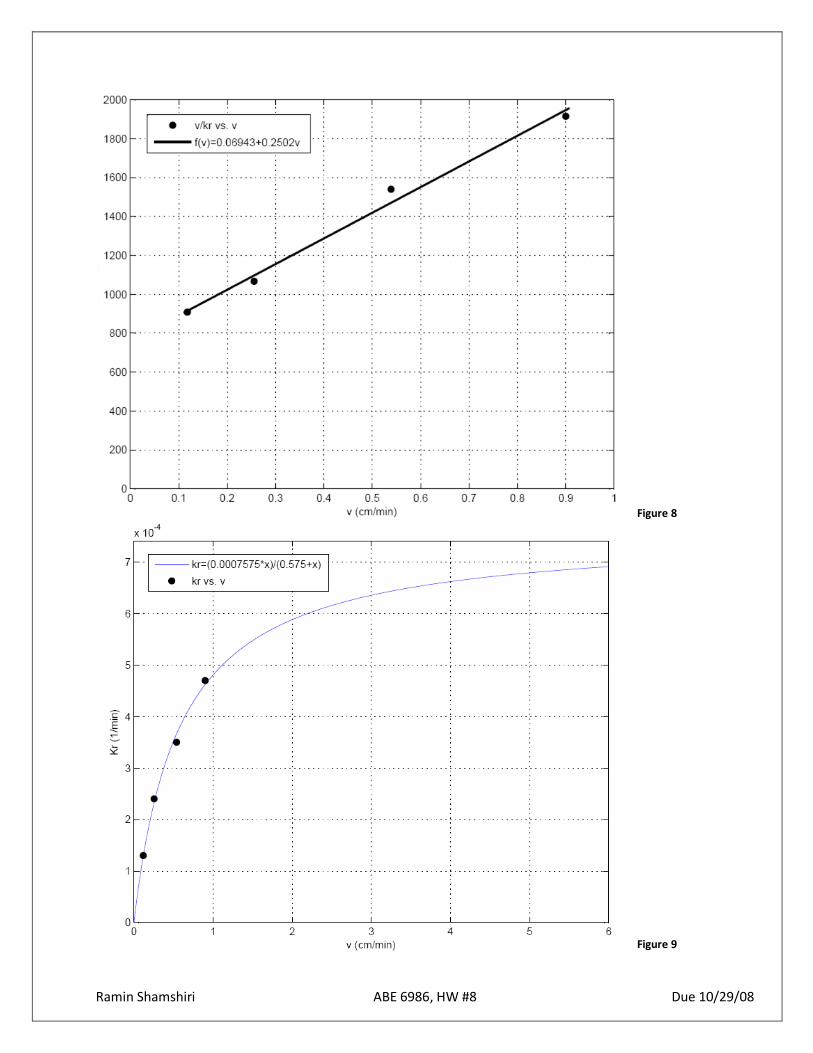
Ramin Shamshiri ABE 6986, HW #8 Due 10/29/08
Figure 8
Figure 9
Ramin Shamshiri ABE 6986, HW #8 Due 10/29/08
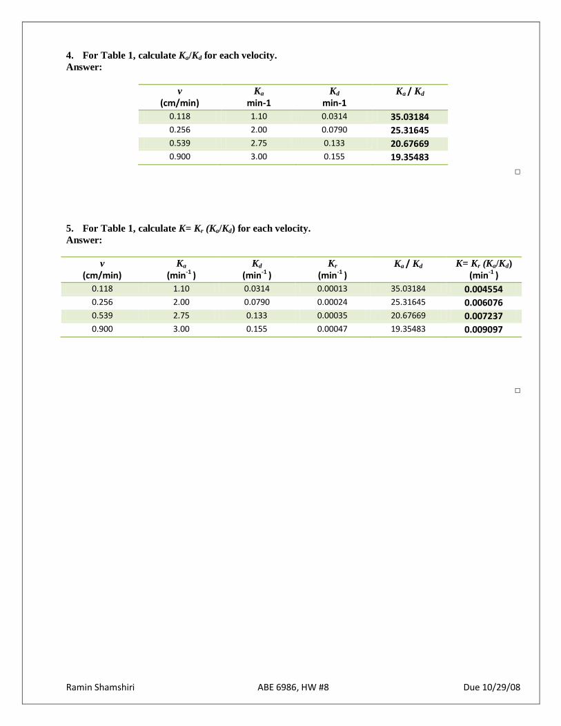
4. For Table 1, calculate Ka/Kd for each velocity.
Answer:
v
(cm/min) Ka
min-1 Kd
min-1 Ka / Kd
0.118 1.10 0.0314 35.03184 0.256 2.00 0.0790 25.31645 0.539 2.75 0.133 20.67669 0.900 3.00 0.155 19.35483
□
5. For Table 1, calculate K= Kr (Ka/Kd) for each velocity.
Answer:
v
(cm/min) Ka
(min-1 ) Kd
(min-1 ) Kr
(min-1 ) Ka / Kd
K= Kr (Ka/Kd)
(min-1 )
0.118 1.10 0.0314 0.00013 35.03184 0.004554 0.256 2.00 0.0790 0.00024 25.31645 0.006076 0.539 2.75 0.133 0.00035 20.67669 0.007237 0.900 3.00 0.155 0.00047 19.35483 0.009097
□
Ramin Shamshiri ABE 6986, HW #8 Due 10/29/08
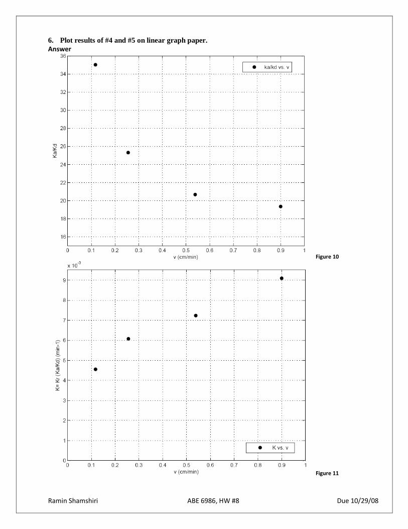
6. Plot results of #4 and #5 on linear graph paper.
Answer
Figure 10
Figure 11

Ramin Shamshiri ABE 6986, HW #8 Due 10/29/08
7. Use regression equations for Ka and Kd to calculate and draw the curve for Ka/Kd vs. v.
Answer:
Approach No.1
𝒌𝒂 =𝒂𝒗
𝒃 + 𝒗=
𝟑.𝟗𝟗𝟔𝟖𝒗
𝟎.𝟐𝟕𝟕𝟒𝟗 + 𝒗
𝒌𝒅 =𝒂𝒗
𝒃 + 𝒗=
𝟎.𝟑𝟒𝟑𝟔𝒗
𝟎.𝟗𝟗𝟒𝟖 + 𝒗
𝒌𝒂
𝒌𝒅 =
𝟑.𝟗𝟗𝟔𝟖𝒗𝟎.𝟐𝟕𝟕𝟒𝟗 + 𝒗
𝟎.𝟑𝟒𝟑𝟔𝒗𝟎.𝟗𝟗𝟒𝟖 + 𝒗
=𝟑. 𝟗𝟕𝟔 + 𝟑. 𝟗𝟗𝟔𝟖𝒗
𝟎.𝟎𝟗𝟓𝟑𝟒 + 𝟎.𝟑𝟒𝟑𝟔𝒗
Figure 12
Ramin Shamshiri ABE 6986, HW #8 Due 10/29/08
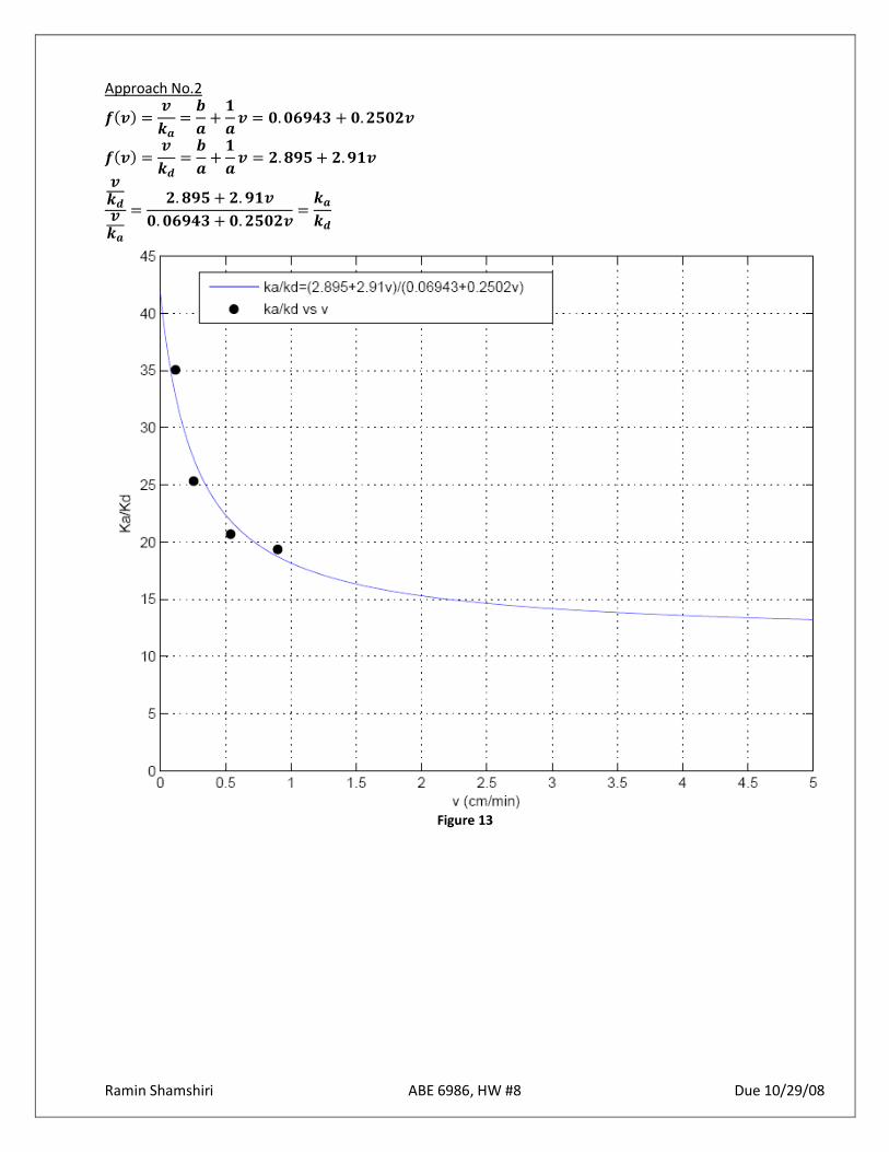
Approach No.2
𝒇 𝒗 =𝒗
𝒌𝒂=
𝒃
𝒂+
𝟏
𝒂𝒗 = 𝟎.𝟎𝟔𝟗𝟒𝟑 + 𝟎.𝟐𝟓𝟎𝟐𝒗
𝒇 𝒗 =𝒗
𝒌𝒅=
𝒃
𝒂+
𝟏
𝒂𝒗 = 𝟐.𝟖𝟗𝟓 + 𝟐.𝟗𝟏𝒗
𝒗𝒌𝒅𝒗𝒌𝒂
=𝟐. 𝟖𝟗𝟓 + 𝟐. 𝟗𝟏𝒗
𝟎. 𝟎𝟔𝟗𝟒𝟑 + 𝟎. 𝟐𝟓𝟎𝟐𝒗=
𝒌𝒂
𝒌𝒅
Figure 13
Ramin Shamshiri ABE 6986, HW #8 Due 10/29/08
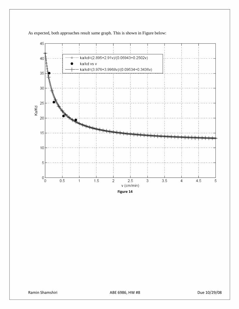
As expected, both approaches result same graph. This is shown in Figure below:
Figure 14
Ramin Shamshiri ABE 6986, HW #8 Due 10/29/08
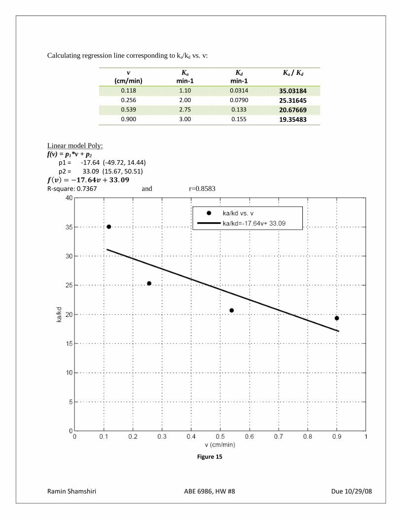
Calculating regression line corresponding to ka/kd vs. v:
v
(cm/min) Ka
min-1 Kd
min-1 Ka / Kd
0.118 1.10 0.0314 35.03184 0.256 2.00 0.0790 25.31645 0.539 2.75 0.133 20.67669 0.900 3.00 0.155 19.35483
Linear model Poly:
f(v) = p1*v + p2
p1 = -17.64 (-49.72, 14.44) p2 = 33.09 (15.67, 50.51) 𝒇 𝒗 = −𝟏𝟕.𝟔𝟒𝒗 + 𝟑𝟑.𝟎𝟗
R-square: 0.7367 and r=0.8583
Figure 15
Ramin Shamshiri ABE 6986, HW #8 Due 10/29/08
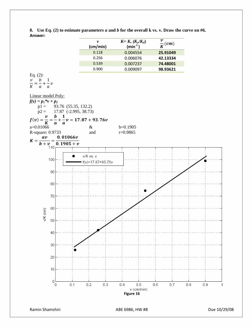
8. Use Eq. (2) to estimate parameters a and b for the overall k vs. v. Draw the curve on #6.
Answer:
v
(cm/min) K= Kr (Ka/Kd)
(min-1 )
𝒗
𝑲(𝒄𝒎)
0.118 0.004554 25.91049 0.256 0.006076 42.13334 0.539 0.007237 74.48001 0.900 0.009097 98.93621
Eq. (2): 𝑣
𝐾=
𝑏
𝑎+
1
𝑎𝑣
Linear model Poly:
f(v) = p1*v + p2
p1 = 93.76 (55.35, 132.2) p2 = 17.87 (-2.995, 38.73)
𝒇 𝒗 =𝒗
𝑲=
𝒃
𝒂+
𝟏
𝒂𝒗 = 𝟏𝟕.𝟖𝟕 + 𝟗𝟑. 𝟕𝟔𝒗
a=0.01066 & b=0.1905
R-square: 0.9733 and r=0.9865
𝑲 =𝒂𝒗
𝒃 + 𝒗=
𝟎. 𝟎𝟏𝟎𝟔𝟔𝒗
𝟎. 𝟏𝟗𝟎𝟓 + 𝒗
Figure 16

Ramin Shamshiri ABE 6986, HW #8 Due 10/29/08
𝑲 =𝒂𝒗
𝒃 + 𝒗=
𝟎. 𝟎𝟏𝟎𝟔𝟔𝒗
𝟎. 𝟏𝟗𝟎𝟓 + 𝒗
Figure 17
Ramin Shamshiri ABE 6986, HW #8 Due 10/29/08
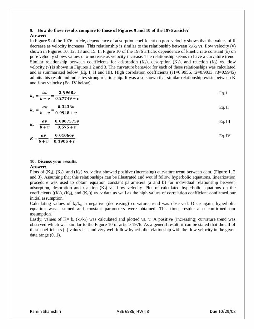
9. How do these results compare to those of Figures 9 and 10 of the 1976 article?
Answer:
In Figure 9 of the 1976 article, dependence of adsorption coefficient on pore velocity shows that the values of R
decrease as velocity increases. This relationship is similar to the relationship between ka/kd vs. flow velocity (v)
shown in Figures 10, 12, 13 and 15. In Figure 10 of the 1976 article, dependence of kinetic rate constant (k) on pore velocity shows values of k increase as velocity increase. The relationship seems to have a curvature trend.
Similar relationship between coefficients for adsorption (Ka), desorption (Kd), and reaction (Kr) vs. flow
velocity (v) is shown in Figures 1,2 and 3. The curvature behavior for each of these relationships was calculated and is summarized below (Eq. I, II and III). High correlation coefficients (r1=0.9956, r2=0.9033, r3=0.9945)
admits this result and indicates strong relationship. It was also shown that similar relationship exists between K
and flow velocity (Eq. IV below).
𝒌𝒂 =𝒂𝒗
𝒃 + 𝒗=
𝟑. 𝟗𝟗𝟔𝟖𝒗
𝟎.𝟐𝟕𝟕𝟒𝟗 + 𝒗
Eq. I
𝒌𝒅 =𝒂𝒗
𝒃 + 𝒗=
𝟎. 𝟑𝟒𝟑𝟔𝒗
𝟎. 𝟗𝟗𝟒𝟖 + 𝒗
Eq. II
𝒌𝒓 =𝒂𝒗
𝒃 + 𝒗=
𝟎. 𝟎𝟎𝟎𝟕𝟓𝟕𝟓𝒗
𝟎. 𝟓𝟕𝟓 + 𝒗
Eq. III
𝑲 =𝒂𝒗
𝒃 + 𝒗=
𝟎.𝟎𝟏𝟎𝟔𝟔𝒗
𝟎. 𝟏𝟗𝟎𝟓 + 𝒗
Eq. IV
10. Discuss your results.
Answer: Plots of (Ka), (Kd), and (Kr ) vs. v first showed positive (increasing) curvature trend between data. (Figure 1, 2
and 3). Assuming that this relationships can be illustrated and would follow hyperbolic equations, linearization
procedure was used to obtain equation constant parameters (a and b) for individual relationship between
adsorption, desorption and reaction (Kr) vs. flow velocity. Plot of calculated hyperbolic equations on the coefficients ((Ka), (Kd), and (Kr )) vs. v data as well as the high values of correlation coefficient confirmed our
initial assumption.
Calculating values of ka/kd, a negative (decreasing) curvature trend was observed. Once again, hyperbolic equation was assumed and constant parameters were obtained. This time, results also confirmed our
assumption.
Lastly, values of K= kr (ka/kd) was calculated and plotted vs. v. A positive (increasing) curvature trend was
observed which was similar to the Figure 10 of article 1976. As a general result, it can be stated that the all of these coefficients (k) values has and very well follow hyperbolic relationship with the flow velocity in the given
data range (0, 1).

Ramin Shamshiri ABE 6986, HW #9 Due 11/07/08
Homework #9
Due 11/07/08
Phosphorus kinetics in a batch reactor
For the work of Burgoa et al. (1990) with a soil/solution ratio of 0.500 kg L-1
we estimate ka=0.050 L mg-
1h
-1, kd=0.25h
-1, kr=0.005h
-1, S0=220mgL
-1. Assume P0=101.8mgL
-1 and A0=0.00mgL
-1.
The kinetic equation become
𝒕 > 0 𝒅𝒑
𝒅𝒕= −𝟎.𝟎𝟓𝟎𝑺𝑷 + 𝟎.𝟐𝟓𝑨
𝒅𝑨
𝒅𝒕= −𝟎.𝟎𝟓𝟎𝑺𝑷 − 𝟎.𝟐𝟓𝟓𝑨
𝑺 = 𝟐𝟐𝟎.𝟎𝟎 − 𝑨
𝒕 = 𝟎 𝑷𝟎 = 𝟏𝟎𝟏.𝟖𝒎𝒈𝑳−𝟏, 𝑨𝟎 = 𝟎, 𝑺𝟎 = 𝟐𝟐𝟎.𝟎𝟎𝒎𝒈𝑳−𝟏
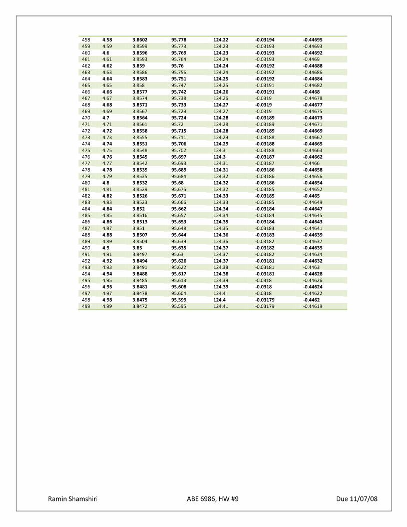
1- Use the Euler method of numerical integration to estimate P, A and S with time.
Answer:
Euler method;
To solve the differential equation of the form below using Euler method, 𝑑𝑦
𝑑𝑥= 𝑓(𝑥,𝑦)
Starting at the initial condition (x0,y0), we will have:
𝑦𝑛+1 = 𝑦𝑛 + (𝑑𝑦
𝑑𝑥)𝑛(𝑥𝑛+1 − 𝑥𝑛)
Here we are given
t > 0 dp
dt= −0.050SP + 0.25A
dA
dt= −0.050SP − 0.255A
S = 220.00 − A
Which can be written in the below form
𝑡 > 0 𝑑𝑃
𝑑𝑡= −ka SP + kd𝐴
𝑑𝐴
𝑑𝑡== −kaSP − kd𝐴 − kr𝐴
𝑆 = S0 − 𝐴
This corresponds to the following numerical solution:
𝑃𝑛+1 = 𝑃𝑛 + (𝑑𝑃
𝑑𝑡)𝑛(∆𝑡𝑛)
𝐴𝑛+1 = 𝐴𝑛 + (𝑑𝐴
𝑑𝑡)𝑛(∆𝑡𝑛)
Sn = S0 − An
Ramin Shamshiri ABE 6986, HW #9 Due 11/07/08
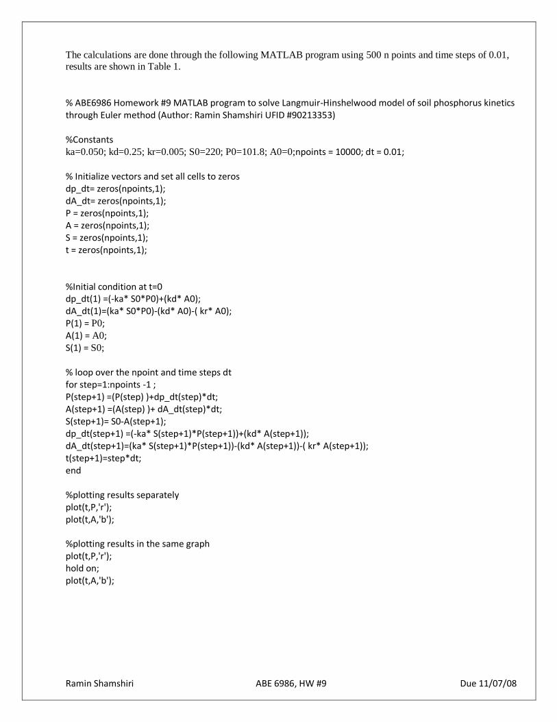
The calculations are done through the following MATLAB program using 500 n points and time steps of 0.01,
results are shown in Table 1.
% ABE6986 Homework #9 MATLAB program to solve Langmuir-Hinshelwood model of soil phosphorus kinetics through Euler method (Author: Ramin Shamshiri UFID #90213353) %Constants ka=0.050; kd=0.25; kr=0.005; S0=220; P0=101.8; A0=0;npoints = 10000; dt = 0.01; % Initialize vectors and set all cells to zeros dp_dt= zeros(npoints,1); dA_dt= zeros(npoints,1); P = zeros(npoints,1); A = zeros(npoints,1); S = zeros(npoints,1); t = zeros(npoints,1); %Initial condition at t=0 dp_dt(1) =(-ka* S0*P0)+(kd* A0); dA_dt(1)=(ka* S0*P0)-(kd* A0)-( kr* A0); P(1) = P0; A(1) = A0; S(1) = S0; % loop over the npoint and time steps dt for step=1:npoints -1 ; P(step+1) =(P(step) )+dp_dt(step)*dt; A(step+1) =(A(step) )+ dA_dt(step)*dt; S(step+1)= S0-A(step+1); dp_dt(step+1) =(-ka* S(step+1)*P(step+1))+(kd* A(step+1)); dA_dt(step+1)=(ka* S(step+1)*P(step+1))-(kd* A(step+1))-( kr* A(step+1)); t(step+1)=step*dt; end %plotting results separately plot(t,P,'r'); plot(t,A,'b'); %plotting results in the same graph plot(t,P,'r'); hold on; plot(t,A,'b');

Ramin Shamshiri ABE 6986, HW #9 Due 11/07/08
n t h
Pn
𝑀𝑔𝐿−1
An
𝑀𝑔𝐿−1
Sn
𝑀𝑔𝐿−1
(dp/dt)n
𝑴𝒈𝑳−𝟏−𝟏
(dA/dt)n
𝑴𝒈𝑳−𝟏−𝟏 0 0 101.8 0 220 -1119.8 1119.8 1 0.01 90.602 11.198 208.8 -943.09 943.04 2 0.02 81.171 20.628 199.37 -804 803.9 3 0.03 73.131 28.667 191.33 -692.45 692.31 4 0.04 66.207 35.59 184.41 -601.56 601.38 5 0.05 60.191 41.604 178.4 -526.49 526.28 6 0.06 54.926 46.867 173.13 -463.76 463.52 7 0.07 50.288 51.502 168.5 -410.8 410.54 8 0.08 46.18 55.608 164.39 -365.68 365.41 9 0.09 42.524 59.262 160.74 -326.94 326.65 10 0.1 39.254 62.528 157.47 -293.44 293.13 11 0.11 36.32 65.46 154.54 -264.28 263.95 12 0.12 33.677 68.099 151.9 -238.75 238.41 13 0.13 31.289 70.483 149.52 -216.29 215.94 14 0.14 29.127 72.643 147.36 -196.44 196.08 15 0.15 27.162 74.603 145.4 -178.81 178.44 16 0.16 25.374 76.388 143.61 -163.1 162.72 17 0.17 23.743 78.015 141.99 -149.05 148.66 18 0.18 22.252 79.502 140.5 -136.45 136.05 19 0.19 20.888 80.862 139.14 -125.1 124.7 20 0.2 19.637 82.109 137.89 -114.86 114.45 21 0.21 18.488 83.254 136.75 -105.6 105.18 22 0.22 17.432 84.305 135.69 -97.198 96.776 23 0.23 16.46 85.273 134.73 -89.565 89.138 24 0.24 15.565 86.165 133.84 -82.615 82.184 25 0.25 14.739 86.986 133.01 -76.275 75.84 26 0.26 13.976 87.745 132.26 -70.483 70.044 27 0.27 13.271 88.445 131.55 -65.182 64.74 28 0.28 12.619 89.093 130.91 -60.324 59.879 29 0.29 12.016 89.691 130.31 -55.866 55.418 30 0.3 11.457 90.246 129.75 -51.77 51.319 31 0.31 10.94 90.759 129.24 -48.003 47.549 32 0.32 10.46 91.234 128.77 -44.533 44.077 33 0.33 10.014 91.675 128.32 -41.335 40.877 34 0.34 9.6009 92.084 127.92 -38.385 37.924 35 0.35 9.217 92.463 127.54 -35.66 35.198 36 0.36 8.8604 92.815 127.18 -33.142 32.678 37 0.37 8.529 93.142 126.86 -30.813 30.348 38 0.38 8.2209 93.445 126.55 -28.658 28.191 39 0.39 7.9343 93.727 126.27 -26.663 26.194 40 0.4 7.6677 93.989 126.01 -24.813 24.343 41 0.41 7.4195 94.233 125.77 -23.099 22.628 42 0.42 7.1886 94.459 125.54 -21.508 21.036 43 0.43 6.9735 94.669 125.33 -20.032 19.559 44 0.44 6.7732 94.865 125.14 -18.662 18.188 45 0.45 6.5865 95.047 124.95 -17.389 16.914 46 0.46 6.4126 95.216 124.78 -16.206 15.73 47 0.47 6.2506 95.373 124.63 -15.106 14.629 48 0.48 6.0995 95.519 124.48 -14.084 13.606 49 0.49 5.9587 95.655 124.34 -13.133 12.654 50 . . 449
.
.
.
.
.
.
.
.
.
.
.
.
.
.
.
.
.
.
.
.
.
.
.
. 450 4.5 3.8628 95.814 124.19 -0.03197 -0.4471 451 4.51 3.8625 95.809 124.19 -0.03196 -0.44708 452 4.52 3.8622 95.805 124.2 -0.03196 -0.44706 453 4.53 3.8618 95.8 124.2 -0.03196 -0.44705 454 4.54 3.8615 95.796 124.2 -0.03195 -0.44703 455 4.55 3.8612 95.791 124.21 -0.03195 -0.44701 456 4.56 3.8609 95.787 124.21 -0.03194 -0.44699 457 4.57 3.8606 95.782 124.22 -0.03194 -0.44697
Ramin Shamshiri ABE 6986, HW #9 Due 11/07/08
458 4.58 3.8602 95.778 124.22 -0.03194 -0.44695 459 4.59 3.8599 95.773 124.23 -0.03193 -0.44693 460 4.6 3.8596 95.769 124.23 -0.03193 -0.44692 461 4.61 3.8593 95.764 124.24 -0.03193 -0.4469 462 4.62 3.859 95.76 124.24 -0.03192 -0.44688 463 4.63 3.8586 95.756 124.24 -0.03192 -0.44686 464 4.64 3.8583 95.751 124.25 -0.03192 -0.44684 465 4.65 3.858 95.747 124.25 -0.03191 -0.44682 466 4.66 3.8577 95.742 124.26 -0.03191 -0.4468 467 4.67 3.8574 95.738 124.26 -0.0319 -0.44678 468 4.68 3.8571 95.733 124.27 -0.0319 -0.44677 469 4.69 3.8567 95.729 124.27 -0.0319 -0.44675 470 4.7 3.8564 95.724 124.28 -0.03189 -0.44673 471 4.71 3.8561 95.72 124.28 -0.03189 -0.44671 472 4.72 3.8558 95.715 124.28 -0.03189 -0.44669 473 4.73 3.8555 95.711 124.29 -0.03188 -0.44667 474 4.74 3.8551 95.706 124.29 -0.03188 -0.44665 475 4.75 3.8548 95.702 124.3 -0.03188 -0.44663 476 4.76 3.8545 95.697 124.3 -0.03187 -0.44662 477 4.77 3.8542 95.693 124.31 -0.03187 -0.4466 478 4.78 3.8539 95.689 124.31 -0.03186 -0.44658 479 4.79 3.8535 95.684 124.32 -0.03186 -0.44656 480 4.8 3.8532 95.68 124.32 -0.03186 -0.44654 481 4.81 3.8529 95.675 124.32 -0.03185 -0.44652 482 4.82 3.8526 95.671 124.33 -0.03185 -0.4465 483 4.83 3.8523 95.666 124.33 -0.03185 -0.44649 484 4.84 3.852 95.662 124.34 -0.03184 -0.44647 485 4.85 3.8516 95.657 124.34 -0.03184 -0.44645 486 4.86 3.8513 95.653 124.35 -0.03184 -0.44643 487 4.87 3.851 95.648 124.35 -0.03183 -0.44641 488 4.88 3.8507 95.644 124.36 -0.03183 -0.44639 489 4.89 3.8504 95.639 124.36 -0.03182 -0.44637 490 4.9 3.85 95.635 124.37 -0.03182 -0.44635 491 4.91 3.8497 95.63 124.37 -0.03182 -0.44634 492 4.92 3.8494 95.626 124.37 -0.03181 -0.44632 493 4.93 3.8491 95.622 124.38 -0.03181 -0.4463 494 4.94 3.8488 95.617 124.38 -0.03181 -0.44628 495 4.95 3.8485 95.613 124.39 -0.0318 -0.44626 496 4.96 3.8481 95.608 124.39 -0.0318 -0.44624 497 4.97 3.8478 95.604 124.4 -0.0318 -0.44622 498 4.98 3.8475 95.599 124.4 -0.03179 -0.4462 499 4.99 3.8472 95.595 124.41 -0.03179 -0.44619
Ramin Shamshiri ABE 6986, HW #9 Due 11/07/08
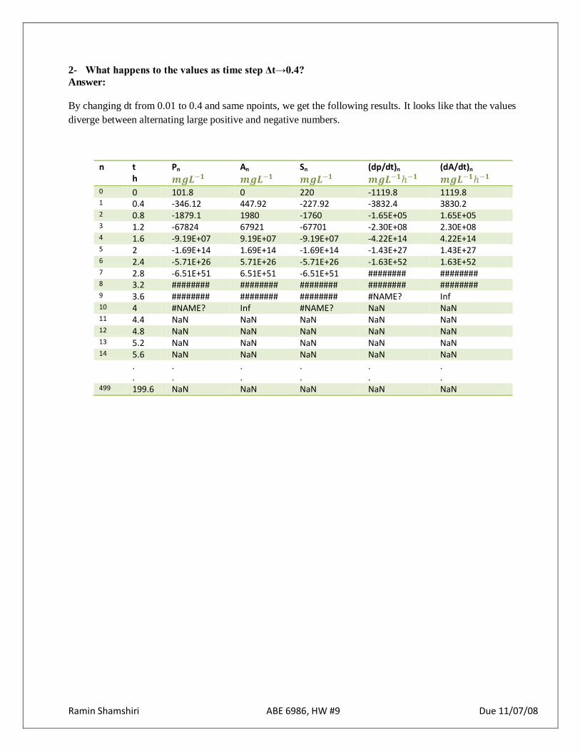
2- What happens to the values as time step Δt→0.4?
Answer:
By changing dt from 0.01 to 0.4 and same npoints, we get the following results. It looks like that the values
diverge between alternating large positive and negative numbers.
n t h
Pn
𝒎𝒈𝑳−𝟏
An
𝒎𝒈𝑳−𝟏
Sn
𝒎𝒈𝑳−𝟏
(dp/dt)n
𝒎𝒈𝑳−𝟏−𝟏
(dA/dt)n
𝒎𝒈𝑳−𝟏−𝟏 0 0 101.8 0 220 -1119.8 1119.8 1 0.4 -346.12 447.92 -227.92 -3832.4 3830.2 2 0.8 -1879.1 1980 -1760 -1.65E+05 1.65E+05 3 1.2 -67824 67921 -67701 -2.30E+08 2.30E+08 4 1.6 -9.19E+07 9.19E+07 -9.19E+07 -4.22E+14 4.22E+14 5 2 -1.69E+14 1.69E+14 -1.69E+14 -1.43E+27 1.43E+27 6 2.4 -5.71E+26 5.71E+26 -5.71E+26 -1.63E+52 1.63E+52 7 2.8 -6.51E+51 6.51E+51 -6.51E+51 ######## ######## 8 3.2 ######## ######## ######## ######## ######## 9 3.6 ######## ######## ######## #NAME? Inf 10 4 #NAME? Inf #NAME? NaN NaN 11 4.4 NaN NaN NaN NaN NaN 12 4.8 NaN NaN NaN NaN NaN 13 5.2 NaN NaN NaN NaN NaN 14 5.6 NaN NaN NaN NaN NaN .
. . .
.
. . .
.
. . .
499 199.6 NaN NaN NaN NaN NaN
Ramin Shamshiri ABE 6986, HW #9 Due 11/07/08
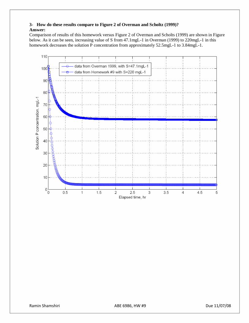
3- How do these results compare to Figure 2 of Overman and Scholtz (1999)?
Answer: Comparison of results of this homework versus Figure 2 of Overman and Scholts (1999) are shown in Figure
below. As it can be seen, increasing value of S from 47.1mgL-1 in Overman (1999) to 220mgL-1 in this
homework decreases the solution P concentration from approximately 52.5mgL-1 to 3.84mgL-1.
Ramin Shamshiri ABE 6986, HW #9 Due 11/07/08
Ramin Shamshiri ABE 6986, HW #9 Due 11/07/08
4- Compare the values of ka, S0, kd and kr.
Answer: The three values of ka, S0, kd and kr are the same in this homework and what has presented in Overman and
Scholtz (1999) work.
5- How does the Langmuir-Hinshelwood model explain the rapid drop in P with time during the initial
phase?
Answer:
The Langmuir-Hinshelwood model provides excellent simulation of batch kinetics for this system. The most
important concern in utilizing this model is being careful in choosing Δt which is required for this system of
equations. Different values of Δt leads to different results which in some cases divergence occur.
6- For the case of large S0 and small P0, is it reasonable to treat S as a constant? Explain.
Answer:
Yes, it is reasonable. To test this, the value of S0 was selected 2200 and small P0 was set at 1.8. The results
showed that after 3 n points, the values of S became constant and equal to 2198.2. This is due to the nature of
the model and algorithm used to determine the answer. According to below:
Sn = S0 − An
𝐴𝑛+1 = 𝐴𝑛 + (𝑑𝐴
𝑑𝑡)𝑛(∆𝑡𝑛)
𝑑𝐴
𝑑𝑡== −kaSP − kd𝐴 − kr𝐴
When S0 is very large and P0 is very small, the values of A0 also becomes small as number of n points increase,
which leads to small difference between S and S0.
Ramin Shamshiri ABE 6986, HW #10 Due 11/14/08
Homework #10
Due 11/14/08
ABE 6986
Ramin Shamshiri
UFID # 90213353
Linearized form of phosphorus kinetics in a batch reactor
For the Linearized model we obtained the solution
𝝋 =𝑷
𝑷𝟎= 𝟏 −
𝒌𝒅
𝒌𝒂 𝒆𝒙𝒑 −𝒌𝒂𝒕 +
𝒌𝒅
𝒌𝒂𝒆𝒙𝒑(−𝒌𝒓𝒕)
Eq.13
We also showed that
𝑨 =𝒌𝒂
𝒔+ 𝒌𝒅 + 𝒌𝒓𝑷
Eq.4

Ramin Shamshiri ABE 6986, HW #10 Due 11/14/08
1. Show that the solution for A(t) is given by
𝑨
𝑷𝟎= 𝟏 −
𝒌𝒅
𝒌𝒂 𝒆𝒙𝒑 − 𝒌𝒅 + 𝒌𝒓 𝒕 − 𝒆𝒙𝒑 −𝒌𝒂𝒕 + {𝒆𝒙𝒑 −𝒌𝒓𝒕 − 𝒆𝒙𝒑 − 𝒌𝒅 + 𝒌𝒓 𝒕 }
Answer:
We have from the handout:
𝑃
𝑃0= 1 −
𝑘𝑑𝑘𝑎
.1
𝑠 + 𝑘𝑎+𝑘𝑑𝑘𝑎.
1
𝑠 + 𝑘𝑟
Dividing both sides of Eq.4 by P0, we will have
𝐴
𝑃0=
𝑘𝑎𝑠 + 𝑘𝑑 + 𝑘𝑟
𝑃
𝑃0
=𝑘𝑎
𝑠 + 𝑘𝑑 + 𝑘𝑟. 1−
𝑘𝑑𝑘𝑎
.1
𝑠 + 𝑘𝑎+𝑘𝑑𝑘𝑎.
1
𝑠 + 𝑘𝑟
= 𝑘𝑎
𝑠 + 𝑘𝑑 + 𝑘𝑟 (𝑠 + 𝑘𝑎) −
𝑘𝑑 𝑠 + 𝑘𝑑 + 𝑘𝑟 (𝑠 + 𝑘𝑎)
+ (𝑘𝑑
𝑠 + 𝑘𝑑 + 𝑘𝑟 (𝑠 + 𝑘𝑟))
=𝐴
[𝑠 + (𝑘𝑑 + 𝑘𝑟)]+
𝐵
𝑠 + 𝑘𝑎 −
𝐶
[𝑠 + (𝑘𝑑 + 𝑘𝑟)]+
𝐷
𝑠 + 𝑘𝑎 +
𝐸
[𝑠 + (𝑘𝑑 + 𝑘𝑟)]+
𝐹
𝑠 + 𝑘𝑟
Assuming ka>>kd + kr we get the below values after partial fraction calculation:
A= 1
B= -1
𝐶 =𝑘𝑑𝑘𝑎
𝐷 = −𝑘𝑑𝑘𝑎
E= -1
F= 1
Therefore we will have:
=1
[𝑠 + (𝑘𝑑 + 𝑘𝑟)]−
1
𝑠 + 𝑘𝑎 −
𝑘𝑑𝑘𝑎
[𝑠 + (𝑘𝑑 + 𝑘𝑟)]−
𝑘𝑑𝑘𝑎
𝑠 + 𝑘𝑎 −
1
[𝑠 + (𝑘𝑑 + 𝑘𝑟)]+
1
𝑠 + 𝑘𝑟
= −1
𝑠 + 𝑘𝑎 −
𝑘𝑑𝑘𝑎
[𝑠 + (𝑘𝑑 + 𝑘𝑟)]−
𝑘𝑑𝑘𝑎
𝑠 + 𝑘𝑎 +
1
𝑠 + 𝑘𝑟
From inverse Laplace transform we know that:
ℒ−1 𝑘
𝑠 + 𝑎 = 𝑘𝑒−𝑎𝑡
(k is a constant)
Ramin Shamshiri ABE 6986, HW #10 Due 11/14/08
ℒ−1 1
𝑠 + 𝑘𝑎 = 𝑒−𝑘𝑎 𝑡
ℒ−1
𝑘𝑑𝑘𝑎
[𝑠+ (𝑘𝑑 + 𝑘𝑟)] =
𝑘𝑑𝑘𝑎
𝑒−(𝑘𝑑+𝑘𝑟 )𝑡
ℒ−1
𝑘𝑑𝑘𝑎
𝑠+ 𝑘𝑎 =
𝑘𝑑𝑘𝑎
𝑒−𝑘𝑎 𝑡
ℒ−1 1
𝑠 + 𝑘𝑟 = 𝑒−𝑘𝑟 𝑡
ℒ−1 𝐴
𝑃0 = −𝑒−𝑘𝑎 𝑡 −
𝑘𝑑𝑘𝑎
𝑒−(𝑘𝑑+𝑘𝑟 )𝑡 −𝑘𝑑𝑘𝑎
𝑒−𝑘𝑎 𝑡 + 𝑒−𝑘𝑟 𝑡
Which is the same as the given equation.
□
2. Show that the solution satisfies the initial condition A=0 at t=0.
Answer:
At t=0 we have:
𝑒𝑥𝑝 − 𝑘𝑑 + 𝑘𝑟 𝑡 = 𝑒𝑥𝑝 0 = 1
𝑒𝑥𝑝 −𝑘𝑎 𝑡 = 𝑒𝑥𝑝 0 = 1
𝑒𝑥𝑝 −𝑘𝑟𝑡 = 𝑒𝑥𝑝 0 = 1
𝑒𝑥𝑝 − 𝑘𝑑 + 𝑘𝑟 𝑡 = 𝑒𝑥𝑝 0 = 1
Thus:
𝐴
𝑃0= 1 −
𝑘𝑑𝑘𝑎
𝑒𝑥𝑝 − 𝑘𝑑 + 𝑘𝑟 𝑡 − 𝑒𝑥𝑝 −𝑘𝑎 𝑡 + 𝑒𝑥𝑝 −𝑘𝑟𝑡 − 𝑒𝑥𝑝 − 𝑘𝑑 + 𝑘𝑟 𝑡
1−𝑘𝑑𝑘𝑎
× 1− 1 + 1 − 1 = 0
□
Ramin Shamshiri ABE 6986, HW #10 Due 11/14/08
3. Show that the solution converges to A→0 as t→∞.
Answer:
limt→∞
𝑒 − 𝑘𝑑+𝑘𝑟 𝑡 = 0
limt→∞
𝑒 −𝑘𝑎 𝑡 = 0
limt→∞
𝑒 −𝑘𝑟 𝑡 = 0
limt→∞
𝑒 − 𝑘𝑑+𝑘𝑟 𝑡 = 0
Thus:
limt→∞
1 −𝑘𝑑𝑘𝑎
𝑒 − 𝑘𝑑+𝑘𝑟 𝑡 − 𝑒 −𝑘𝑎 𝑡 + 𝑒 −𝑘𝑟 𝑡 − 𝑒 − 𝑘𝑑+𝑘𝑟 𝑡
= 1−𝑘𝑑𝑘𝑎
× 0 + 0 + 0 = 0
□
Ramin Shamshiri ABE 6986, HW #11 Due 11/21/08
Homework #11
Due 11/21/08
ABE 6986
Ramin Shamshiri
UFID # 90213353
Numerical integration of a PDE by the implicit method
Consider the hear conduction problem discussed in the handout.
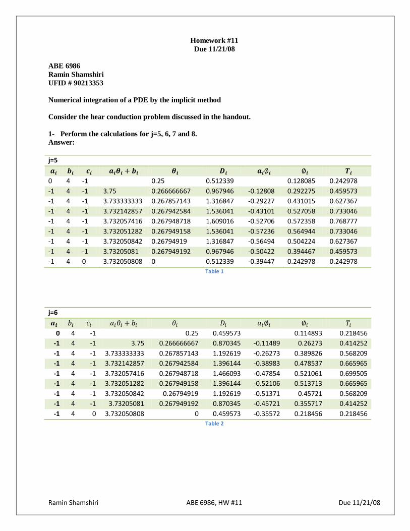
1- Perform the calculations for j=5, 6, 7 and 8.
Answer:
j=5
𝒂𝒊 𝒃𝒊 𝒄𝒊 𝒂𝒊𝜽𝒊 + 𝒃𝒊 𝜽𝒊 𝑫𝒊 𝒂𝒊∅𝒊 ∅𝒊 𝑻𝒊
0 4 -1 0.25 0.512339 0.128085 0.242978
-1 4 -1 3.75 0.266666667 0.967946 -0.12808 0.292275 0.459573
-1 4 -1 3.733333333 0.267857143 1.316847 -0.29227 0.431015 0.627367
-1 4 -1 3.732142857 0.267942584 1.536041 -0.43101 0.527058 0.733046
-1 4 -1 3.732057416 0.267948718 1.609016 -0.52706 0.572358 0.768777
-1 4 -1 3.732051282 0.267949158 1.536041 -0.57236 0.564944 0.733046
-1 4 -1 3.732050842 0.26794919 1.316847 -0.56494 0.504224 0.627367
-1 4 -1 3.73205081 0.267949192 0.967946 -0.50422 0.394467 0.459573
-1 4 0 3.732050808 0 0.512339 -0.39447 0.242978 0.242978
Table 1
j=6
𝒂𝒊 𝑏𝑖 𝑐𝑖 𝑎𝑖𝜃𝑖 + 𝑏𝑖 𝜃𝑖 𝐷𝑖 𝑎𝑖∅𝑖 ∅𝑖 𝑇𝑖
0 4 -1 0.25 0.459573 0.114893 0.218456
-1 4 -1 3.75 0.266666667 0.870345 -0.11489 0.26273 0.414252
-1 4 -1 3.733333333 0.267857143 1.192619 -0.26273 0.389826 0.568209
-1 4 -1 3.732142857 0.267942584 1.396144 -0.38983 0.478537 0.665965
-1 4 -1 3.732057416 0.267948718 1.466093 -0.47854 0.521061 0.699505
-1 4 -1 3.732051282 0.267949158 1.396144 -0.52106 0.513713 0.665965
-1 4 -1 3.732050842 0.26794919 1.192619 -0.51371 0.45721 0.568209
-1 4 -1 3.73205081 0.267949192 0.870345 -0.45721 0.355717 0.414252
-1 4 0 3.732050808 0 0.459573 -0.35572 0.218456 0.218456
Table 2

Ramin Shamshiri ABE 6986, HW #11 Due 11/21/08
j=7
𝒂𝒊 𝑏𝑖 𝑐𝑖 𝑎𝑖𝜃𝑖 + 𝑏𝑖 𝜃𝑖 𝐷𝑖 𝑎𝑖∅𝑖 ∅𝑖 𝑇𝑖
0 4 -1 0.25 0.414252 0.103563 0.197234
-1 4 -1 3.75 0.266666667 0.786665 -0.10356 0.237394 0.374683
-1 4 -1 3.733333333 0.267857143 1.080217 -0.23739 0.352932 0.514834
-1 4 -1 3.732142857 0.267942584 1.267714 -0.35293 0.43424 0.604437
-1 4 -1 3.732057416 0.267948718 1.331929 -0.43424 0.473243 0.635201
-1 4 -1 3.732051282 0.267949158 1.267714 -0.47324 0.466488 0.604437
-1 4 -1 3.732050842 0.26794919 1.080217 -0.46649 0.414438 0.514834
-1 4 -1 3.73205081 0.267949192 0.786665 -0.41444 0.321835 0.374683
-1 4 0 3.732050808 0 0.414252 -0.32183 0.197234 0.197234
Table 3
j=8
𝒂𝒊 𝑏𝑖 𝑐𝑖 𝑎𝑖𝜃𝑖 + 𝑏𝑖 𝜃𝑖 𝐷𝑖 𝑎𝑖∅𝑖 ∅𝑖 𝑇𝑖
0 4 -1 0.25 0.374683 0.093671 0.178498
-1 4 -1 3.75 0.266666667 0.712068 -0.09367 0.214864 0.33931
-1 4 -1 3.733333333 0.267857143 0.979121 -0.21486 0.319817 0.466674
-1 4 -1 3.732142857 0.267942584 1.150035 -0.31982 0.393836 0.548265
-1 4 -1 3.732057416 0.267948718 1.208875 -0.39384 0.429444 0.576351
-1 4 -1 3.732051282 0.267949158 1.150035 -0.42944 0.42322 0.548265
-1 4 -1 3.732050842 0.26794919 0.979121 -0.42322 0.375756 0.466674
-1 4 -1 3.73205081 0.267949192 0.712068 -0.37576 0.291482 0.33931
-1 4 0 3.732050808 0 0.374683 -0.29148 0.178498 0.178498
Table 4
Ramin Shamshiri ABE 6986, HW #11 Due 11/21/08
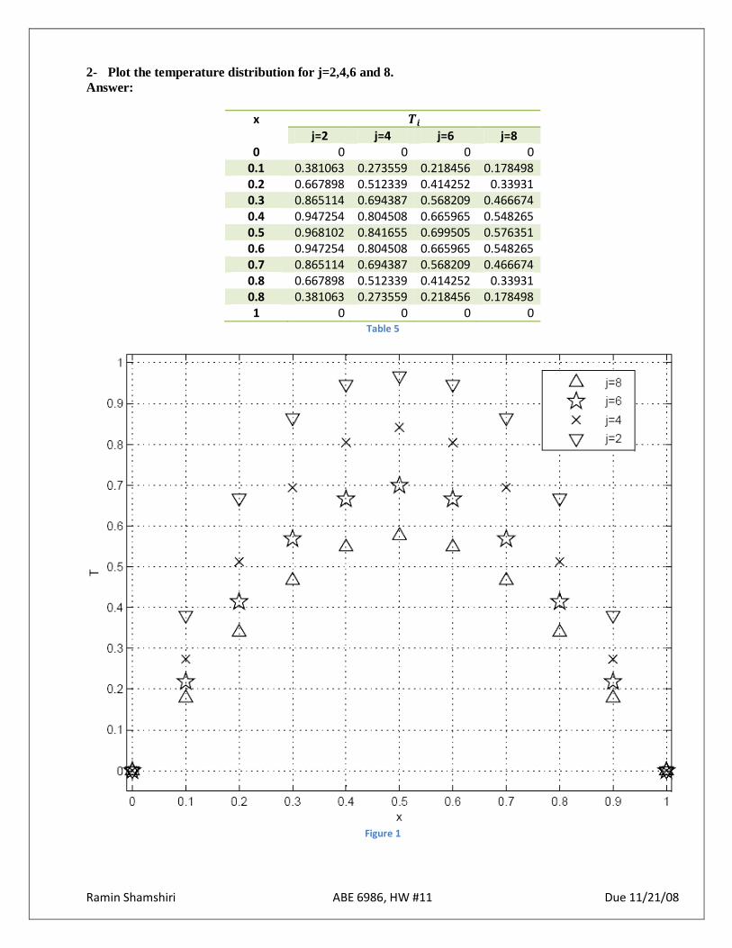
2- Plot the temperature distribution for j=2,4,6 and 8.
Answer:
x 𝑻𝒊
j=2 j=4 j=6 j=8 0 0 0 0 0
0.1 0.381063 0.273559 0.218456 0.178498 0.2 0.667898 0.512339 0.414252 0.33931 0.3 0.865114 0.694387 0.568209 0.466674 0.4 0.947254 0.804508 0.665965 0.548265 0.5 0.968102 0.841655 0.699505 0.576351 0.6 0.947254 0.804508 0.665965 0.548265 0.7 0.865114 0.694387 0.568209 0.466674 0.8 0.667898 0.512339 0.414252 0.33931 0.8 0.381063 0.273559 0.218456 0.178498 1 0 0 0 0
Table 5
Figure 1
Ramin Shamshiri ABE 6986, HW #11 Due 11/21/08
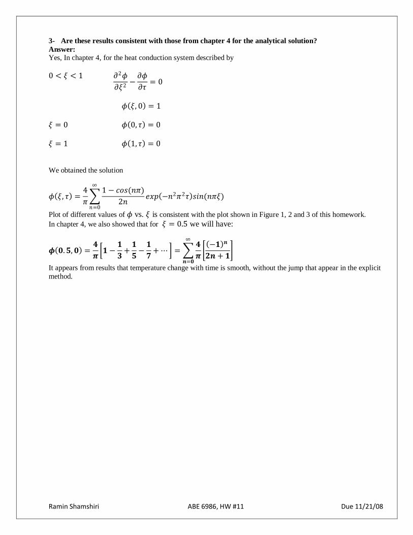
3- Are these results consistent with those from chapter 4 for the analytical solution?
Answer: Yes, In chapter 4, for the heat conduction system described by
0 < 𝜉 < 1 𝜕2𝜙
𝜕𝜉2−
𝜕𝜙
𝜕𝜏= 0
𝜙 𝜉, 0 = 1
𝜉 = 0 𝜙 0, 𝜏 = 0
𝜉 = 1 𝜙 1, 𝜏 = 0
We obtained the solution
𝜙 𝜉, 𝜏 =4
𝜋
1 − 𝑐𝑜𝑠(𝑛𝜋)
2𝑛
∞
𝑛=0
𝑒𝑥𝑝 −𝑛2𝜋2𝜏 𝑠𝑖𝑛(𝑛𝜋𝜉)
Plot of different values of 𝜙 vs. 𝜉 is consistent with the plot shown in Figure 1, 2 and 3 of this homework.
In chapter 4, we also showed that for 𝜉 = 0.5 we will have:
𝝓 𝟎. 𝟓, 𝟎 =𝟒
𝝅 𝟏 −
𝟏
𝟑+
𝟏
𝟓−
𝟏
𝟕+ ⋯ =
𝟒
𝝅 −𝟏 𝒏
𝟐𝒏 + 𝟏
∞
𝒏=𝟎
It appears from results that temperature change with time is smooth, without the jump that appear in the explicit
method.
Ramin Shamshiri ABE 6986, HW #11 Due 11/21/08
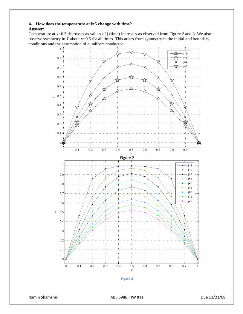
4- How does the temperature at i=5 change with time?
Answer: Temperature at x=0.5 decreases as values of j (time) increases as observed from Figure 2 and 3. We also
observe symmetry in T about x=0.5 for all times. This arises from symmetry in the initial and boundary
conditions and the assumption of a uniform conductor.
Figure 2
Figure 3
Ramin Shamshiri ABE 6986, MIDTERM EXAM Due 10/03/08
Midterm Exam
Due 10/03/08
ABE 6986
Ramin Shamshiri
UFID # 90213353
Consider the discrete logistic model given by
𝑑𝜑
𝑑𝜏≅
∆∅
∆𝜏= ∅ 1 − ∅ → ∆∅𝑛 = ∅𝑛(1 − ∅𝑛)∆𝜏𝑛
∅𝑛+1 = ∅𝑛 + ∆∅𝑛 with ∅ = ∅0 = 0.1000 at 𝜏 = 0
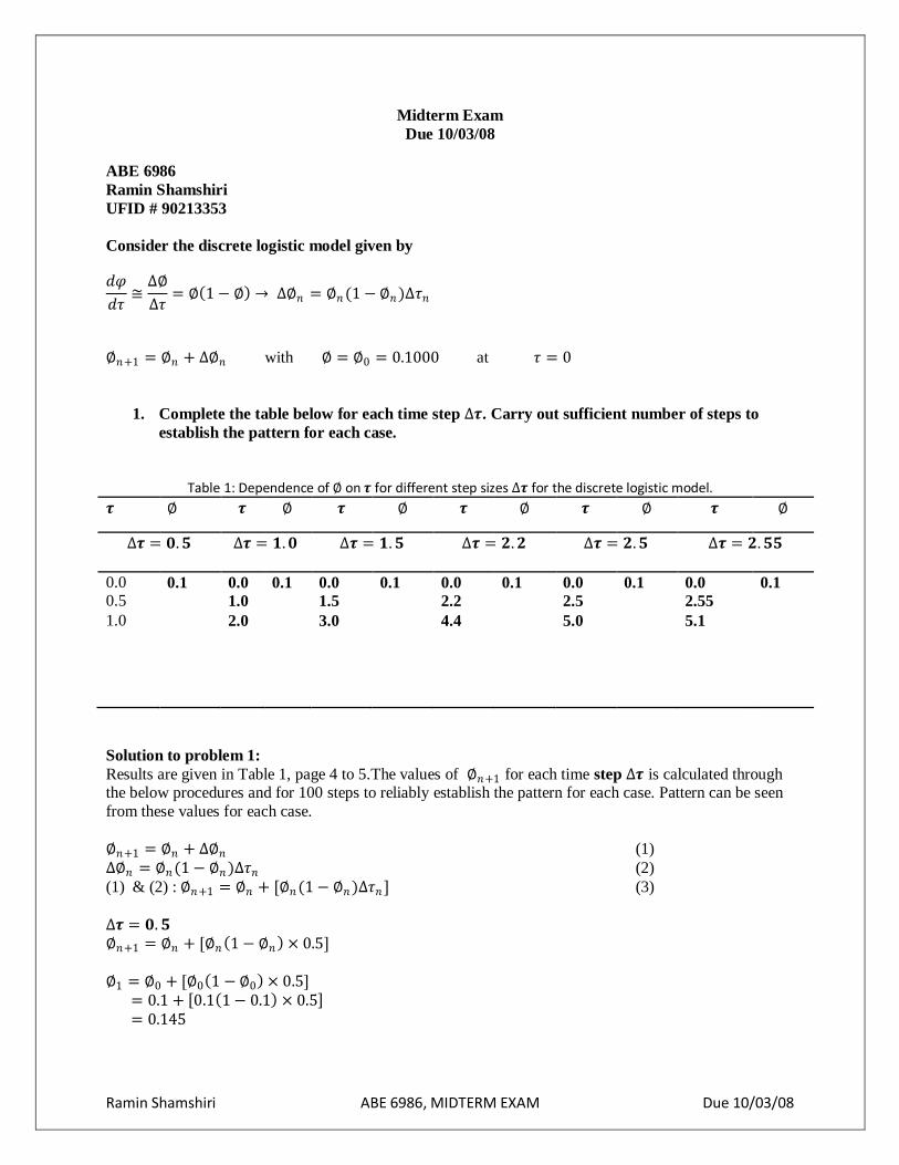
1. Complete the table below for each time step ∆𝝉. Carry out sufficient number of steps to
establish the pattern for each case.
Table 1: Dependence of ∅ on 𝝉 for different step sizes ∆𝝉 for the discrete logistic model.
𝝉 ∅ 𝝉 ∅ 𝝉 ∅ 𝝉 ∅ 𝝉 ∅ 𝝉 ∅
∆𝝉 = 𝟎. 𝟓 ∆𝝉 = 𝟏. 𝟎 ∆𝝉 = 𝟏. 𝟓 ∆𝝉 = 𝟐. 𝟐 ∆𝝉 = 𝟐. 𝟓 ∆𝝉 = 𝟐. 𝟓𝟓
0.0 0.1 0.0 0.1 0.0 0.1 0.0 0.1 0.0 0.1 0.0 0.1 0.5 1.0 1.5 2.2 2.5 2.55
1.0 2.0 3.0 4.4 5.0 5.1
Solution to problem 1:
Results are given in Table 1, page 4 to 5.The values of ∅𝑛+1 for each time step ∆𝝉 is calculated through the below procedures and for 100 steps to reliably establish the pattern for each case. Pattern can be seen
from these values for each case.
∅𝑛+1 = ∅𝑛 + ∆∅𝑛 (1)
∆∅𝑛 = ∅𝑛(1 − ∅𝑛)∆𝜏𝑛 (2)
(1) & (2) : ∅𝑛+1 = ∅𝑛 + [∅𝑛(1 − ∅𝑛)∆𝜏𝑛 ] (3)
∆𝝉 = 𝟎. 𝟓
∅𝑛+1 = ∅𝑛 + [∅𝑛 1 − ∅𝑛 × 0.5]
∅1 = ∅0 + [∅0 1 − ∅0 × 0.5]
= 0.1 + 0.1 1 − 0.1 × 0.5 = 0.145
Ramin Shamshiri ABE 6986, MIDTERM EXAM Due 10/03/08
∅2 = ∅1 + [∅1 1 − ∅1 × 0.5] = 0.145 + 0.145 1 − 0.145 × 0.5 = 0.2069875
∅3 = ∅2 + [∅2 1 − ∅2 × 0.5] = 0.2069875 + 0.2069875 1 − 0.2069875 × 0.5 = 0.289059337 .
.
.
∆𝝉 = 𝟏. 𝟎
∅𝑛+1 = ∅𝑛 + [∅𝑛 1 − ∅𝑛 × 1.0]
∅1 = ∅0 + [∅0 1 − ∅0 × 1.0]
= 0.1 + 0.1 1 − 0.1 × 1.0 = 0.19
∅2 = ∅1 + [∅1 1 − ∅1 × 1.0] = 0.19 + 0.19 1 − 0.19 × 1.0 = 0.3439
∅3 = ∅2 + [∅2 1 − ∅2 × 1.0] = 0.3439 + 0.3439 1 − 0.3439 × 1.0 = 0.56953279
.
.
.
∆𝝉 = 𝟏. 𝟓
∅𝑛+1 = ∅𝑛 + [∅𝑛 1 − ∅𝑛 × 1.5]
∅1 = ∅0 + [∅0 1 − ∅0 × 1.5]
= 0.1 + 0.1 1 − 0.1 × 1.5 = 0.235
∅2 = ∅1 + [∅1 1 − ∅1 × 1.5] = 0.235 + 0.235 1 − 0.2355 × 1.5 = 0.5046625
∅3 = ∅2 + [∅2 1 − ∅2 × 1.5] = 0.5046625 + 0.5046625 1 − 0.5046625 × 1.5 = 0.879629891640625 .
.
.
Ramin Shamshiri ABE 6986, MIDTERM EXAM Due 10/03/08
∆𝝉 = 𝟐. 𝟐
∅𝑛+1 = ∅𝑛 + [∅𝑛 1 − ∅𝑛 × 2.2]
∅1 = ∅0 + [∅0 1 − ∅0 × 2.2]
= 0.1 + 0.1 1 − 0.1 × 2.2 = 0.298
∅2 = ∅1 + [∅1 1 − ∅1 × 2.2] = 0.298 + 0.298 1 − 0.298 × 2.2 = 0.7582312
∅3 = ∅2 + [∅2 1 − ∅2 × 0.5] = 0.7582312 + 0.7582312 1 − 0.7582312 × 2.2 = 1.16152782416243 .
.
.
∆𝝉 = 𝟐. 𝟓
∅𝑛+1 = ∅𝑛 + [∅𝑛 1 − ∅𝑛 × 2.5]
∅1 = ∅0 + [∅0 1 − ∅0 × 2.5]
= 0.1 + 0.1 1 − 0.1 × 2.5 = 0.325
∅2 = ∅1 + [∅1 1 − ∅1 × 2.5] = 0.325 + 0.325 1 − 0.325 × 2.5 = 0.8734375
∅3 = ∅2 + [∅2 1 − ∅2 × 2.5] = 0.8734375 + 0.8734375 1 − 0.8734375 × 2.5 = 1.14979858398437 .
.
.
∆𝝉 = 𝟐. 𝟓𝟓
∅𝑛+1 = ∅𝑛 + [∅𝑛 1 − ∅𝑛 × 2.55]
∅1 = ∅0 + [∅0 1 − ∅0 × 2.55] = 0.1 + 0.1 1 − 0.1 × 2.55 = 0.3295
∅2 = ∅1 + [∅1 1 − ∅1 × 2.55] = 0.3295 + 0.3295 1 − 0.3295 × 2.55 = 0.8928708625
∅3 = ∅2 + [∅2 1 − ∅2 × 0.5] = 0.8928708625 + 0.8928708625 1 − 0.8928708625 × 2.55 = 1.13678470026619 .
Ramin Shamshiri ABE 6986, MIDTERM EXAM Due 10/03/08
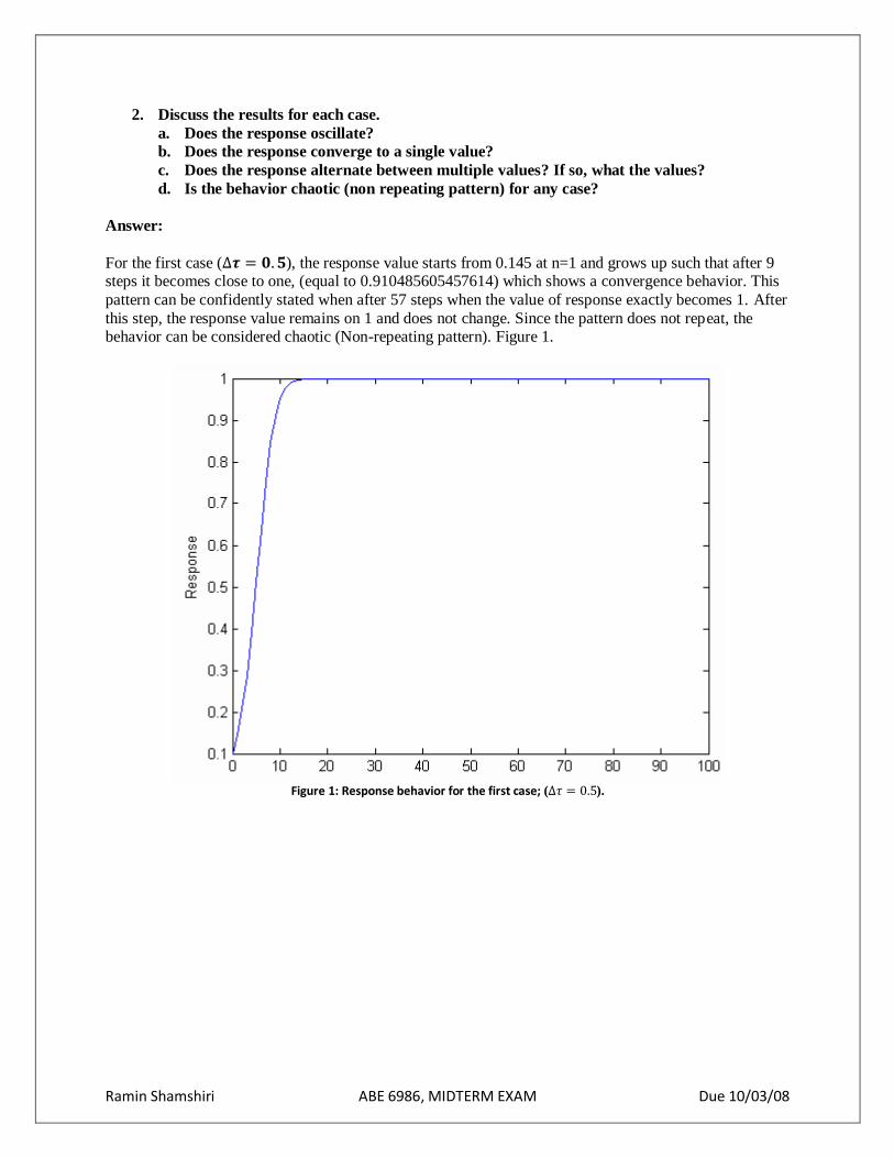
2. Discuss the results for each case.
a. Does the response oscillate?
b. Does the response converge to a single value?
c. Does the response alternate between multiple values? If so, what the values?
d. Is the behavior chaotic (non repeating pattern) for any case?
Answer:
For the first case (∆𝝉 = 𝟎. 𝟓), the response value starts from 0.145 at n=1 and grows up such that after 9 steps it becomes close to one, (equal to 0.910485605457614) which shows a convergence behavior. This
pattern can be confidently stated when after 57 steps when the value of response exactly becomes 1. After
this step, the response value remains on 1 and does not change. Since the pattern does not repeat, the behavior can be considered chaotic (Non-repeating pattern). Figure 1.
Figure 1: Response behavior for the first case; (∆𝜏 = 0.5).
Ramin Shamshiri ABE 6986, MIDTERM EXAM Due 10/03/08
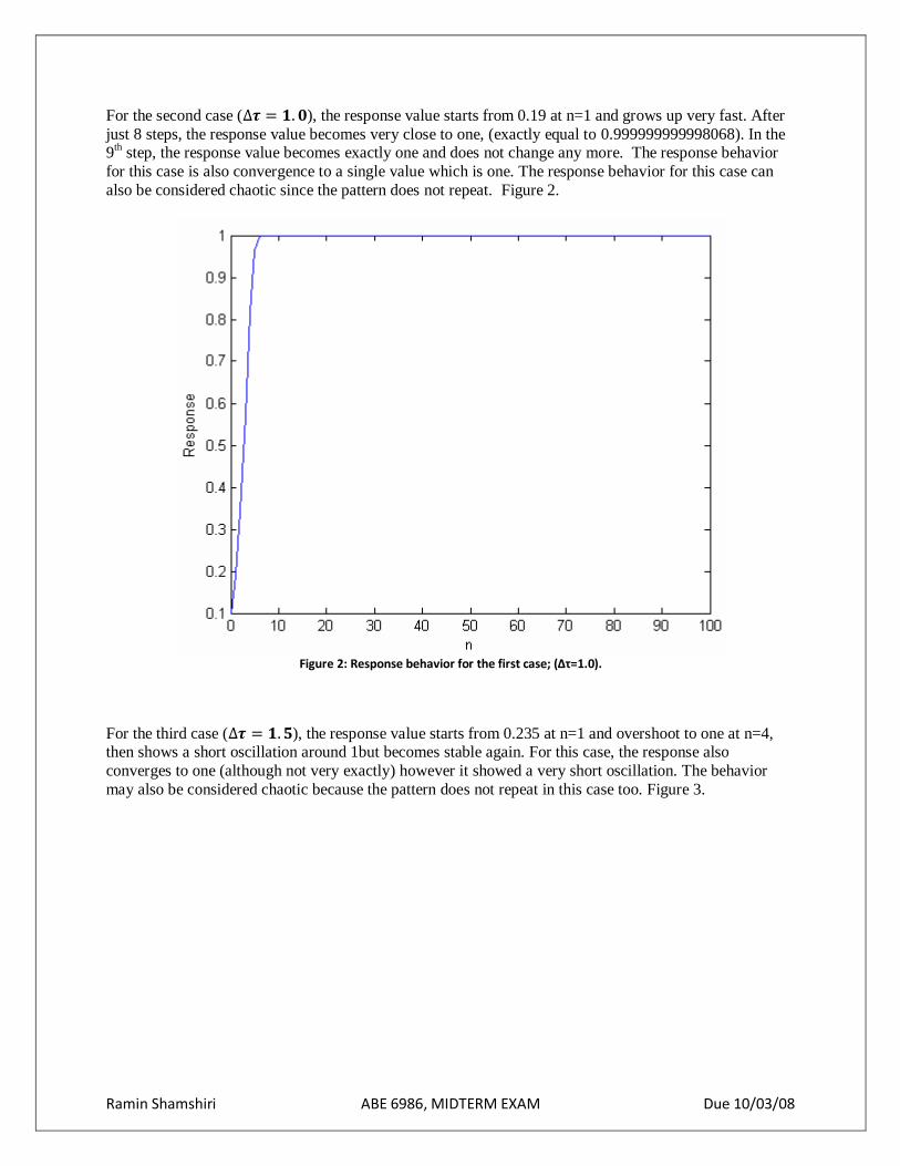
For the second case (∆𝝉 = 𝟏. 𝟎), the response value starts from 0.19 at n=1 and grows up very fast. After
just 8 steps, the response value becomes very close to one, (exactly equal to 0.999999999998068). In the 9
th step, the response value becomes exactly one and does not change any more. The response behavior
for this case is also convergence to a single value which is one. The response behavior for this case can
also be considered chaotic since the pattern does not repeat. Figure 2.
Figure 2: Response behavior for the first case; (∆τ=1.0).
For the third case (∆𝝉 = 𝟏. 𝟓), the response value starts from 0.235 at n=1 and overshoot to one at n=4, then shows a short oscillation around 1but becomes stable again. For this case, the response also
converges to one (although not very exactly) however it showed a very short oscillation. The behavior
may also be considered chaotic because the pattern does not repeat in this case too. Figure 3.
Ramin Shamshiri ABE 6986, MIDTERM EXAM Due 10/03/08
Figure 3: Response behavior for the first case; (∆τ=1.5).
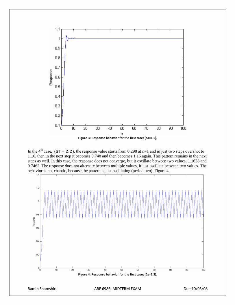
In the 4th case, (∆𝝉 = 𝟐. 𝟐), the response value starts from 0.298 at n=1 and in just two steps overshot to
1.16, then in the next step it becomes 0.748 and then becomes 1.16 again. This pattern remains in the next
steps as well. In this case, the response does not converge, but it oscillate between two values, 1.1628 and
0.7462. The response does not alternate between multiple values, it just oscillate between two values. The
behavior is not chaotic, because the pattern is just oscillating (period two). Figure 4.
Figure 4: Response behavior for the first case; (∆τ=2.2).

Ramin Shamshiri ABE 6986, MIDTERM EXAM Due 10/03/08
In the 5th cases, (∆τ = 2.5), the response oscillate between four values (does not converge). Yes the
response alternate between multiple values (four values) which are 1.157, 0.7012, 1.22, and 0.535. In this case, the behavior is not chaotic. It is just alternating periodically (period 4). Figure 5.
Figure 5: Response behavior for the first case; (∆τ=2.5).
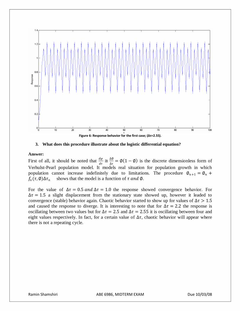
In the 5th cases, (∆τ = 2.55), the response oscillate between four values (does not converge). Yes the
response alternate between multiple values (eight values) which are 1.1523, 0.7047, 1.2353, 0.4939,
1.1313, 0.7523, 1.2274, 0.5154. In this case, the behavior is not chaotic. It is just alternating periodically (period 8). Figure 6.
Ramin Shamshiri ABE 6986, MIDTERM EXAM Due 10/03/08
Figure 6: Response behavior for the first case; (∆τ=2.55).
3. What does this procedure illustrate about the logistic differential equation?
Answer:
First of all, it should be noted that 𝑑𝜑
𝑑𝜏≅
∆∅
∆𝜏= ∅ 1 − ∅ is the discrete dimensionless form of
Verhulst-Pearl population model. It models real situation for population growth in which
population cannot increase indefinitely due to limitations. The procedure ∅𝑛+1 = ∅𝑛 +𝑓𝑛 (𝜏, ∅)∆𝜏𝑛 shows that the model is a function of 𝜏 𝑎𝑛𝑑 ∅.
For the value of ∆𝜏 = 0.5 𝑎𝑛𝑑 ∆𝜏 = 1.0 the response showed convergence behavior. For
∆𝜏 = 1.5 a slight displacement from the stationary state showed up, however it leaded to
convergence (stable) behavior again. Chaotic behavior started to show up for values of ∆𝜏 > 1.5
and caused the response to diverge. It is interesting to note that for ∆𝜏 = 2.2 the response is
oscillating between two values but for ∆𝜏 = 2.5 and ∆𝜏 = 2.55 it is oscillating between four and
eight values respectively. In fact, for a certain value of ∆𝜏, chaotic behavior will appear where
there is not a repeating cycle.
Copyright © 2022 FDOKUMEN