HAL Id: hal-01241277https://hal.archives-ouvertes.fr/hal-01241277v3

Submitted on 17 Jun 2016

HAL is a multi-disciplinary open accessarchive for the deposit and dissemination of sci-entific research documents, whether they are pub-lished or not. The documents may come fromteaching and research institutions in France orabroad, or from public or private research centers.

L’archive ouverte pluridisciplinaire HAL, estdestinée au dépôt et à la diffusion de documentsscientifiques de niveau recherche, publiés ou non,émanant des établissements d’enseignement et derecherche français ou étrangers, des laboratoirespublics ou privés.

A tutorial on Palm distributions for spatial pointprocesses

Jean-François Coeurjolly, Jesper Møller, Rasmus Waagepetersen

To cite this version:Jean-François Coeurjolly, Jesper Møller, Rasmus Waagepetersen. A tutorial on Palm distribu-tions for spatial point processes. International Statistical Review, Wiley, 2017, 83 (5), pp.404-420�10.1111/insr.12205�. �hal-01241277v3�

A tutorial on Palm distributions for spatial

point processes

Jean-Francois Coeurjolly1, Jesper Møller2 and Rasmus

Waagepetersen2

1Laboratory Jean Kuntzmann, Statistics Department, Grenoble Alpes University,

51 Rue des Mathematiques, Campus de Saint Martin d’Heres, BP 53 - 38041

Grenoble cedex 09, France, email:

Jean-Francois.Coeurjolly@univ-grenoble-alpes.fr.

1Department of Mathematical Sciences, Aalborg University, Fredrik Bajersvej

7E, DK-9220 Aalborg, email: jm@math.aau.dk, rw@math.aau.dk,

June 17, 2016

Abstract

This tutorial provides an introduction to Palm distributions for

spatial point processes. Initially, in the context of finite point pro-

cesses, we give an explicit definition of Palm distributions in terms

of their density functions. Then we review Palm distributions in the

1

general case. Finally we discuss some examples of Palm distributions

for specific models and some applications.

Keywords: determinantal process; Cox process; Gibbs process; joint intensi-

ties; log Gaussian Cox process; Palm likelihood; reduced Palm distribution;

shot noise Cox process; summary statistics.

1 Introduction

A spatial point process X is briefly speaking a random subset of the d-

dimensional Euclidean space Rd, where d = 2, 3 are the cases of most prac-

tical importance. We refer to the (random) elements of X as ‘events’ to

distinguish them from other possibly fixed points in Rd. When studying spa-

tial point process models and making statistical inference, the conditional

distribution of X given a realization of X on some specified region or given

the locations of one or more events in X plays an important role, see e.g.

Møller and Waagepetersen (2004) and Chiu et al. (2013). In this paper we fo-

cus on the latter type of conditional distributions which are formally defined

in terms of so-called Palm distributions, first introduced by Palm (1943) for

stationary point processes on the real line. Rigorous definitions and gener-

alizations of Palm distributions to Rd and more abstract spaces have mainly

been developed in probability theory, see Jagers (1973) for references and

an historical account. Palm distributions are, at least among many applied

statisticians and among most students, considered one of the more difficult

2

topics in the field of spatial point processes. This is partly due to the general

definition of Palm distributions which relies on measure theoretical results,

see e.g. Møller and Waagepetersen (2004) and Daley and Vere-Jones (2008)

or the references mentioned in Section 7. The account of conditional distri-

butions for point processes in Last (1990) is mainly intended for probabilists

and is not easily accessible due to an abstract setting and extensive use of

measure theory.

This tutorial provides an introduction to Palm distributions for spatial

point processes. Our setting and background material on point processes are

given in Section 2. Section 3, in the context of finite point processes, provides

an explicit definition of Palm distributions in terms of their density functions

while Section 4 reviews Palm distributions in the general case. Section 5

discusses examples of Palm distributions for specific models and Section 6

considers applications of Palm distributions in the statistical literature.

2 Prerequisites

2.1 Setting and notation

We view a point process as a random locally finite subset X of a Borel set

S ⊆ Rd; for measure theoretical details, see e.g. Møller and Waagepetersen

(2004) or Daley and Vere-Jones (2003). Denoting XB = X∩B the restriction

of X to a set B ⊆ S, and N(B) the number of events in XB, local finiteness

of X means that N(B) < ∞ almost surely (a.s.) whenever B is bounded.

3

We denote by B0 the family of all bounded Borel subsets of S and by N the

state space consisting of the locally finite subsets (or point configurations)

of S. Section 3 considers the case where S is bounded and hence N is all

finite subsets of S, while Section 4 deals with the general case where S is

arbitrary, i.e., including the case S = Rd.

2.2 Poisson process

The Poisson process is of its own interest and also used for constructing other

point processes as demonstrated in Section 2.3 and Section 5.

Suppose ρ : S 7→ [0,∞) is a locally integrable function, that is, α(B) :=∫

Bρ(x) dx < ∞ whenever B ∈ B0. ThenX is a Poisson process with intensity

function ρ if for any B ∈ B0, N(B) is Poisson distributed with mean α(B),

and conditional on N(B) = n, the n events are independent and identically

distributed, with a density proportional to ρ (if α(B) = 0, then N(B) = 0).

In fact, this definition is equivalent to that for any B ∈ B0 and any non-

negative measurable function h on {x ∩B|x ∈ N},

Eh(XB) =∞∑

n=0

exp{−α(B)}

n!∫

B

· · ·

∫

B

h({x1, . . . , xn})ρ(x1) · · ·ρ(xn) dx1 · · · dxn , (1)

where for n = 0 the term is exp{−α(B)}h(∅), where ∅ is the empty point

configuration.

4

Note that the definition of a Poisson process only requires the existence

of the intensity measure α, since an event of the process restricted to B ∈ B0

has probability distribution α(· ∩B)/α(B) provided α(B) > 0. We shall use

this extension of the definition in Section 5.3.2.

2.3 Finite point processes specified by a density

Let Z denote a unit rate Poisson process on S, i.e. a Poisson process of

constant intensity ρ(u) = 1, u ∈ S. Assume that S is bounded and that the

distribution of X is absolutely continuous with respect to the distribution of

Z (in short with respect to Z) with density f . Thus, for any non-negative

measurable function h on N ,

Eh(X) = E{f(Z)h(Z)}. (2)

Moreover, by (1),

Eh(X) =∞∑

n=0

exp(−|S|)

n!∫

S

· · ·

∫

S

h({x1, . . . , xn})f({x1, . . . , xn}) dx1 · · · dxn (3)

where |S| denotes the Lebesgue measure of S. This motivates considering

probability statements in terms of exp(−|S|)f(·). For example, with h(x) =

1(x = ∅), where 1(·) denotes the indicator function, we obtain that P (X = ∅)

5

is exp(−|S|)f(∅). Further, for n ≥ 1,

exp(−|S|)f({x1, . . . , xn}) dx1 · · · dxn

is the probability that X consists of precisely n events with one event in

each of n infinitesimally small disjoint sets B1, . . . , Bn around x1, . . . , xn

with volumes dx1, . . . dxn, respectively. Loosely speaking this is ‘P (X =

{x1, . . . , xn})’.

Suppose we have observed XB = xB and we wish to predict the remaining

point process XS\B. Then it is natural to consider the conditional distribu-

tion of XS\B given XB = xB. By definition of a Poisson process, ZB and

ZS\B (Z = ZB ∪ ZS\B) are each independent unit rate Poisson processes on

respectively B and S \ B. Thus, in analogy with conditional densities for

multivariate data, this conditional distribution can be specified in terms of

the conditional density

fS\B(xS\B|xB) =f(xB ∪ xS\B)

fB(xB)

with respect to ZS\B and where

fB(xB) = Ef(ZS\B ∪ xB)

is the marginal density ofXB with respect to ZB. Thus the conditional distri-

bution given a realization of X on some prespecified region B is conceptually

6

quite straightforward. Conditioning on that some prespeficied events belong

to X is more intricate but an explicit account of this is provided in the next

section where it is still assumed that X is specified in terms of a density.

3 Palm distributions in the finite case

To understand the definition of a Palm distribution, it is useful to assume

first that S is bounded and that X has a density as introduced in Section 2.3

with respect to a unit rate Poisson process Z. We make this assumption in

the present section, while the general case will be treated in Section 4.

3.1 Conditional intensity and joint intensities

Suppose f is hereditary, i.e., for any pairwise distinct x0, x1, . . . , xn ∈ S,

f({x1, . . . , xn}) > 0 whenever f({x0, x1, . . . , xn}) > 0. We can then define

the so-called n-th order Papangelou conditional intensity by

λ(n)(x1, . . . , xn,x) = f(x ∪ {x1, . . . , xn})/f(x) (4)

for pairwise distinct x1, . . . , xn ∈ S and x ∈ N \{x1, . . . , xn}, setting 0/0 = 0.

By the previous interpretation of f , λ(n)(x1, . . . , xn,x) dx1 · · · dxn can be

considered as the conditional probability of observing one event in each of the

aforementioned infinitesimally small sets Bi, conditional on that X outside

∪ni=1Bi agrees with x.

7

For any n = 1, 2, . . ., we define for pairwise distinct x1, . . . , xn ∈ S the

n-th order joint intensity function ρ(n) by

ρ(n)(x1, . . . , xn) = Ef(Z ∪ {x1, . . . , xn}) (5)

provided the right hand side exists. Particularly, ρ = ρ(1) is the usual inten-

sity function. If f is hereditary, then ρ(n)(x1, . . . , xn) = Eλ(n)(x1, . . . , xn,X)

and by the interpretation of λ(n) it follows that ρ(n)(x1, . . . , xn) dx1 · · · dxn

can be viewed as the probability that X has an event in each of n infinites-

imally small sets around x1, . . . , xn with volumes dx1, . . . dxn, respectively.

Loosely speaking, this is ‘P (x1, . . . , xn ∈ X)’.

Combining (2) and (5) with either (3) or the extended Slivnyak-Mecke

theorem for the Poisson process given later in (17), it is straightforwardly

seen that

E

6=∑

x1,...,xn∈X

h(x1, . . . , xn)

=

∫

S

· · ·

∫

S

h(x1, . . . , xn)ρ(n)(x1, . . . , xn) dx1 . . . dxn (6)

for any non-negative measurable function h on Sn, where 6= over the summa-

tion sign means that x1, . . . , xn are pairwise distinct. Denoting N = N(S)

the number of events in X, the left hand side in (6) with h = 1 is seen to be

the factorial moment E{N(N − 1) · · · (N − n+ 1)}.

8

3.2 Definition of Palm distributions in the finite case

Now, suppose x1, . . . , xn ∈ S are pairwise distinct and ρ(n)(x1, . . . , xn) > 0.

Then we define the reduced Palm distribution of X given events at x1, . . . , xn

as the point process distribution P!x1,...,xn

with density

fx1,...,xn(x) =

f(x ∪ {x1, . . . , xn})

ρ(n)(x1, . . . , xn), x ∈ N , x ∩ {x1, . . . , xn} = ∅, (7)

with respect to Z. We denote by X!x1,...,xn

a point process distributed accord-

ing to P!x1,...,xn

. If x1, . . . , xn ∈ S are not pairwise distinct or ρ(n)(x1, . . . , xn)

is zero, the choice of X!x1,...,xn

and its distribution P!x1,...,xn

is not of any im-

portance for the results in this paper. Furthermore, the (non-reduced) Palm

distribution of X given events at x1, . . . , xn is simply the distribution of the

union X!x1,...,xn

∪ {x1, . . . , xn}.

3.3 Remarks

By the previous infinitesimal interpretations of f and ρ(n), we can view

exp(−|S|)fx1,...,xn(x) as the ‘joint probability’ that X equals the union x ∪

{x1, . . . , xn} divided by the ‘probability’ that x1, . . . , xn ∈ X. Thus P!x1,...,xn

has an interpretation as the conditional distribution of X\{x1, . . . , xn} given

that x1, . . . , xn ∈ X. Conversely, by (7) with x = ∅ and the remark just below

(3),

exp(−|S|)f({x1, . . . , xn}) = ρ(n)(x1, . . . , xn)P(

X!{x1,...,xn} = ∅

)

(8)

9

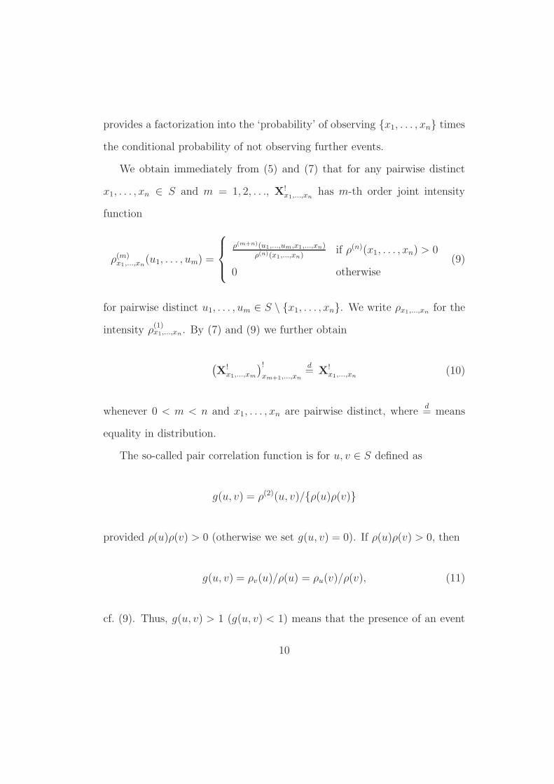
provides a factorization into the ‘probability’ of observing {x1, . . . , xn} times

the conditional probability of not observing further events.

We obtain immediately from (5) and (7) that for any pairwise distinct

x1, . . . , xn ∈ S and m = 1, 2, . . ., X!x1,...,xn

has m-th order joint intensity

function

ρ(m)x1,...,xn

(u1, . . . , um) =

ρ(m+n)(u1,...,um,x1,...,xn)

ρ(n)(x1,...,xn)if ρ(n)(x1, . . . , xn) > 0

0 otherwise(9)

for pairwise distinct u1, . . . , um ∈ S \ {x1, . . . , xn}. We write ρx1,...,xnfor the

intensity ρ(1)x1,...,xn

. By (7) and (9) we further obtain

(

X!x1,...,xm

)!

xm+1,...,xn

d= X!

x1,...,xn(10)

whenever 0 < m < n and x1, . . . , xn are pairwise distinct, whered= means

equality in distribution.

The so-called pair correlation function is for u, v ∈ S defined as

g(u, v) = ρ(2)(u, v)/{ρ(u)ρ(v)}

provided ρ(u)ρ(v) > 0 (otherwise we set g(u, v) = 0). If ρ(u)ρ(v) > 0, then

g(u, v) = ρv(u)/ρ(u) = ρu(v)/ρ(v), (11)

cf. (9). Thus, g(u, v) > 1 (g(u, v) < 1) means that the presence of an event

10

at u yields an elevated (decreased) intensity at v and vice versa.

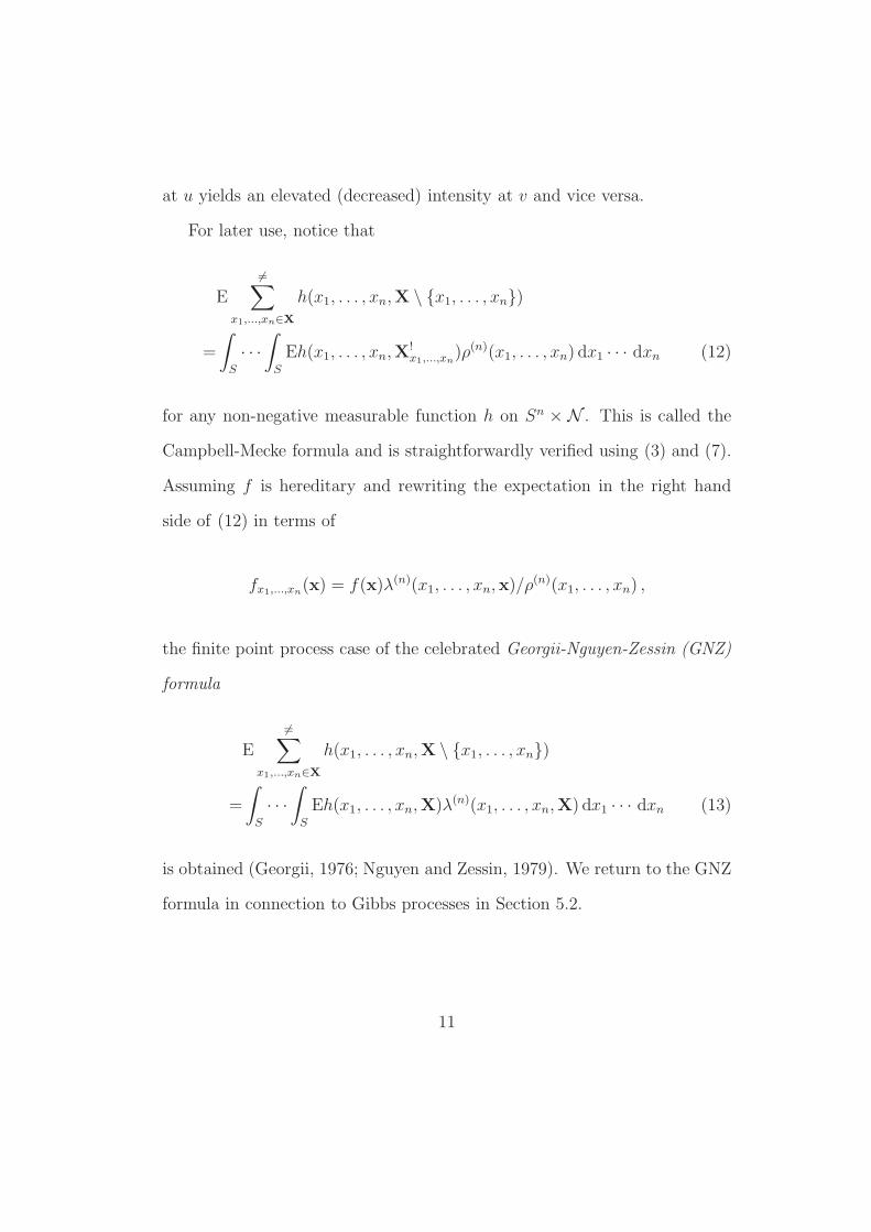
For later use, notice that

E

6=∑

x1,...,xn∈X

h(x1, . . . , xn,X \ {x1, . . . , xn})

=

∫

S

· · ·

∫

S

Eh(x1, . . . , xn,X!x1,...,xn

)ρ(n)(x1, . . . , xn) dx1 · · · dxn (12)

for any non-negative measurable function h on Sn × N . This is called the

Campbell-Mecke formula and is straightforwardly verified using (3) and (7).

Assuming f is hereditary and rewriting the expectation in the right hand

side of (12) in terms of

fx1,...,xn(x) = f(x)λ(n)(x1, . . . , xn,x)/ρ

(n)(x1, . . . , xn) ,

the finite point process case of the celebrated Georgii-Nguyen-Zessin (GNZ)

formula

E

6=∑

x1,...,xn∈X

h(x1, . . . , xn,X \ {x1, . . . , xn})

=

∫

S

· · ·

∫

S

Eh(x1, . . . , xn,X)λ(n)(x1, . . . , xn,X) dx1 · · · dxn (13)

is obtained (Georgii, 1976; Nguyen and Zessin, 1979). We return to the GNZ

formula in connection to Gibbs processes in Section 5.2.

11

4 Palm distributions in the general case

The definitions and results in Section 3 extend to the general case where S

is any Borel subset of Rd. However, if |S| = ∞, the unit rate Poisson process

on S will be infinite and we can not in general assume that X is absolutely

continuous with respect to the distribution of this process. Thus we do not

longer have the direct definitions (5) and (7) of ρ(n) and X!x1,...,xn

in terms of

density functions.

4.1 Definition of Palm distributions in the general case

Define the n-th order factorial moment measure α(n) on Sn by

α(n)(×ni=1Bi) = E

6=∑

x1,...,xn∈X

1(x1 ∈ B1, . . . , xn ∈ Bn)

for Borel sets B1, . . . , Bn ⊆ S. Then provided α(n) is absolutely continuous

with respect to Lebesgue measure on Sn, the n-th order joint intensity for

X is defined as the density of α(n) with respect to Lebesgue measure on

Sn. Then, by standard measure theoretical arguments, (6) also holds in the

general case. Define further the n-th order reduced Campbell measure by

C! (×ni=1Bi × F ) = E

6=∑

x1,...,xn∈X

1(x1 ∈ B1, . . . , xn ∈ Bn,X \ {x1, . . . , xn} ∈ F )

12

for Borel sets B1, . . . , Bn ⊆ S and any measurable set F of point configu-

rations in N . Obviously for any such F , C ! is dominated by α(n), and so,

under suitable regularity conditions (e.g. Section 13.1 in Daley and Vere-

Jones, 2003), we have a disintegration of C!,

C!(×ni=1Bi × F ) =

∫

×n

i=1Bi

P!x1,...,xn

(F )α(n)( dx1 · · · dxn) (14)

where P!x1,...,xn

(F ) is unique up to an α(n) null-set and for almost all x1, . . . , xn ∈

S defines a distribution of a point process X!x1,...,xn

. Again by standard mea-

sure theoretical results, (12) also holds in the general case (if ρ(n) does not

exist, then in (12) replace ρ(n)(x1, . . . , xn) dx1 · · · dxn by α(n)( dx1 · · · dxn)).

In the finite point process case as considered in Section 3, by (12) and (14)

the density approach and the Campbell measure approach to define Palm

distributions agree.

4.2 Remarks

In the general setting, ρ(n)(x1, . . . , xn) and P!x1,...,xn

are clearly only deter-

mined up to an α(n) nullset of Sn. For simplicity and since there are usu-

ally natural choices of ρ(n)(x1, . . . , xn) and P!x1,...,xn

, such nullsets are often

ignored. Further, like in the finite case, ρ(n)(x1, . . . , xn) and P!x1,...,xn

are in-

variant under permutations of the points x1, . . . , xn, and (9) and (10) also

hold in the general case.

Suppose thatX is stationary, i.e., its distribution is invariant under trans-

13

lations in Rd and so S = Rd (unless X = ∅ which is not a case of our interest).

This is a specially tractable case, which makes an alternative description of

Palm distributions possible. Let ρ denote the constant intensity of X and let

o denote the origin in Rd. First, we define

P!o(F ) =

1

ρ|B|E

∑

x∈XB

1(X \ {x} − x ∈ F ) (15)

for any B ∈ B0 with |B| > 0, where by stationarity of X the right hand side

does not depend on the choice of B. Second, we define

P!x(F ) = P!

o(F − x) (16)

for any x ∈ Rd. One can then check that the P!x, x ∈ Rd, defined in this way

satisfy (14) so that (16) indeed defines a Palm distribution, see Appendix C.2

in Møller and Waagepetersen (2004) for details. Note that (16) implies that

X!x − x and X!

o are identically distributed. The reduced Palm distribution

P!o is often interpreted as the ‘conditional distribution for the further events

in X given a typical event of X’.

5 Examples of Palm distributions

For some classes of point processes, explicit characterizations of the Palm

distributions are possible. Below we consider Poisson processes, Gibbs pro-

cesses, log Gaussian Cox processes (LGCPs), and determinantal point pro-

14

cesses which share the property that their Palm distributions of any order

are again respectively Poisson, Gibbs, LGCPs, and determinantal point pro-

cesses. We also consider shot-noise Cox processes, where one point Palm

distributions are not shot-noise Cox processes but have simple characteri-

zations as cluster processes. The section is concluded with Tables 1 and 2

which summarize key characteristics for the different model classes.

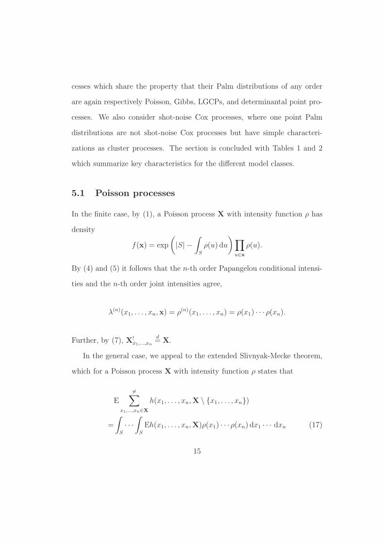
5.1 Poisson processes

In the finite case, by (1), a Poisson process X with intensity function ρ has

density

f(x) = exp

(

|S| −

∫

S

ρ(u) du

)

∏

u∈x

ρ(u).

By (4) and (5) it follows that the n-th order Papangelou conditional intensi-

ties and the n-th order joint intensities agree,

λ(n)(x1, . . . , xn,x) = ρ(n)(x1, . . . , xn) = ρ(x1) · · ·ρ(xn).

Further, by (7), X!x1,...,xn

d= X.

In the general case, we appeal to the extended Slivnyak-Mecke theorem,

which for a Poisson process X with intensity function ρ states that

E

6=∑

x1,...,xn∈X

h(x1, . . . , xn,X \ {x1, . . . , xn})

=

∫

S

· · ·

∫

S

Eh(x1, . . . , xn,X)ρ(x1) · · ·ρ(xn) dx1 · · · dxn (17)

15

for any non-negative measurable function h on Sn × N , see Theorem 3.3

in Møller and Waagepetersen (2004) and the references therein. This im-

plies again that ρ(n)(x1, . . . , xn) = ρ(x1) · · · ρ(xn) and that X!x1,...,xn

is just

distributed as X. In fact, the property that X!x

d= X for all x ∈ S charac-

terizes the Poisson process, see e.g. Proposition 5 in Jagers (1973). Further,

it makes it possible to calculate various useful functional summaries, see

e.g. Møller and Waagepetersen (2004), and constructions such as stationary

Poisson-Voronoi tessellations become manageable, see Møller (1989, 1994).

5.2 Gibbs processes

Gibbs processes play an important role in statistical physics and spatial

statistics, see Møller and Waagepetersen (2004) and the references therein.

Below, for ease of presentation, we consider first a finite Gibbs process.

A finite Gibbs process on a bounded set S ⊂ Rd is usually specified in

terms of its density or equivalently in terms of the Papangelou conditional

intensity, where the density is of the form

f(x) = exp

{

−∑

y⊆x

Φ(y)

}

for a so-called potential function Φ on N , while the Papangelou conditional

intensity is

λ(u,x) = exp

−∑

y⊆x∪{u}: u∈y

Φ(y)

.

16

Here exp{Φ(∅)} is the normalizing constant (partition function) of f(·) which

in general is not expressible on closed form, while λ(u,x) does not depend on

the normalizing constant. It follows that the n-th order Palm distribution of

a Gibbs process with respect to x1, . . . , xn is itself a Gibbs process with poten-

tial function Φx1,...,xn(y) = Φ({x1, . . . , xn}∪y) for y 6= ∅. Moreover, for pair-

wise distinct u1, . . . , um, x1, . . . , xn ∈ S and x ∈ N \{u1, . . . , um, x1, . . . , xn},

the m-th order Papangelou conditional intensity of X!x1,...,xn

is simply

λ!(m)x1,...,xn

(u1, . . . , um,x) = λ(m)(u1, . . . , um,x ∪ {x1, . . . , xn}).

For instance, a first order inhomogeneous pairwise interaction Gibbs point

process has first order potential Φ({u}) = Φ1(u), second order potential

Φ({u, v}) = Φ2(v − u), and Φ(y) = 0 whenever the cardinality of y is

larger than two; see Møller and Waagepetersen (2004) for conditions on the

functions Φ1 and Φ2 ensuring that the model is well-defined. The Strauss

model (Strauss, 1975; Kelly and Ripley, 1976) is a particular case with

Φ1(u) = θ1 ∈ R and Φ2(u − v) = θ21(‖u − v‖ ≤ R), for θ2 ≥ 0 and

0 < R < ∞. The Palm process X!x1,...,xn

becomes again an inhomogeneous

pairwise interaction Gibbs process with inhomogeneous first order potential

Φx1,...,xn({u}) = Φ1(u)+

∑n

i=1Φ2(u−xi) and second order potential identical

to that of X.

In the general case, a Gibbs process can be defined (Nguyen and Zessin,

1979) in terms of the GNZ formula (13) briefly discussed at the end of Sec-

17

tion 3: X is a Gibbs point process with Papangelou conditional intensity λ

if λ is a non-negative measurable function on S ×N such that

E∑

x∈X

h(x,X \ {x}) = E

∫

S

λ(x,X)h(x,X) dx (18)

for any non-negative measurable function h on S×N . For conditions ensuring

that (18) holds, we refer to Ruelle (1969), Georgii (1988), or Dereudre et al.

(2012).

By the extensions of (6) and (12) to the general case, (18) implies ρ(x) =

Eλ(x,X). Unfortunately, in general it is not feasible to express ρ(x) =

Eλ(x,X) on closed form, though approximations exist (Baddeley and Nair,

2012). Also, for Gibbs processes, the pair correlation function g(u, v) can

be below or above 1 depending on u and v (see e.g. pages 240-241 in Illian

et al., 2008), and so from (11), ρv(u) may be smaller or larger than ρ(u),

depending on u and v. Moreover, for pairwise distinct x1, . . . , xn ∈ S, P!x1,...,xn

is absolutely continuous with respect to the distribution of X, with density

f(x) = λ(n)(x1, . . . , xn,x)/ρ(n)(x1, . . . , xn), where

λ(n)(x1, . . . , xn,x) = λ(x1,x)λ(x2,x ∪ {x1})

· · ·λ(xn,x ∪ {x1, . . . , xn−1})

for x1, . . . , xn ∈ S and x ∈ N . This follows from (13) and (18) and is in

accordance with (4) and (10). Note that in this connection, the roles of

18

x and x1, . . . , xn in λ(n)(x1, . . . , xn,x) are interchanged: now x1, . . . , xn are

fixed while x is the variable argument of the density of P!x1,...,xn

.

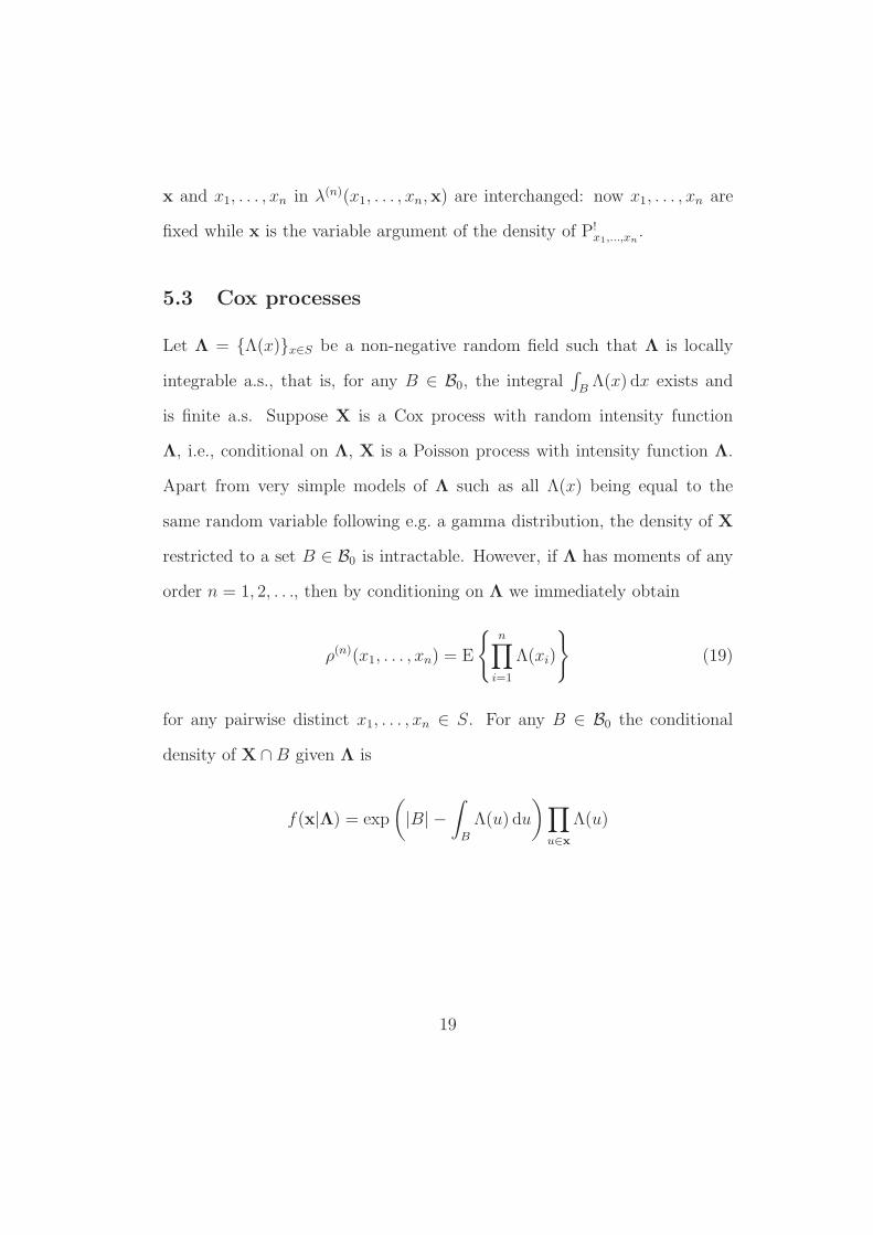
5.3 Cox processes

Let Λ = {Λ(x)}x∈S be a non-negative random field such that Λ is locally

integrable a.s., that is, for any B ∈ B0, the integral∫

BΛ(x) dx exists and

is finite a.s. Suppose X is a Cox process with random intensity function

Λ, i.e., conditional on Λ, X is a Poisson process with intensity function Λ.

Apart from very simple models of Λ such as all Λ(x) being equal to the

same random variable following e.g. a gamma distribution, the density of X

restricted to a set B ∈ B0 is intractable. However, if Λ has moments of any

order n = 1, 2, . . ., then by conditioning on Λ we immediately obtain

ρ(n)(x1, . . . , xn) = E

{

n∏

i=1

Λ(xi)

}

(19)

for any pairwise distinct x1, . . . , xn ∈ S. For any B ∈ B0 the conditional

density of X ∩ B given Λ is

f(x|Λ) = exp

(

|B| −

∫

B

Λ(u) du

)

∏

u∈x

Λ(u)

19

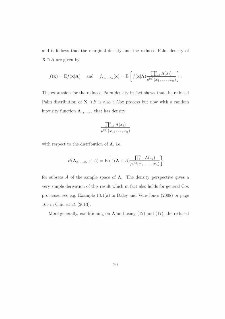
and it follows that the marginal density and the reduced Palm density of

X ∩B are given by

f(x) = Ef(x|Λ) and fx1,...,xn(x) = E

{

f(x|Λ)

∏ni=1 Λ(xi)

ρ(n)(x1, . . . , xn)

}

.

The expression for the reduced Palm density in fact shows that the reduced

Palm distribution of X ∩ B is also a Cox process but now with a random

intensity function Λx1,...,xnthat has density

∏ni=1 Λ(xi)

ρ(n)(x1, . . . , xn)

with respect to the distribution of Λ, i.e.

P (Λx1,...,xn∈ A) = E

{

1(Λ ∈ A)

∏ni=1 Λ(xi)

ρ(n)(x1, . . . , xn)

}

for subsets A of the sample space of Λ. The density perspective gives a

very simple derivation of this result which in fact also holds for general Cox

processes, see e.g. Example 13.1(a) in Daley and Vere-Jones (2008) or page

169 in Chiu et al. (2013).

More generally, conditioning on Λ and using (12) and (17), the reduced

20

Palm distributions satisfy

E{

h(

x1, . . . , xn,X!x1,...,xn

)}

ρ(n)(x1, . . . , xn)

= E

{

h(x1, . . . , xn,X)n∏

i=1

Λ(xi)

}

(20)

for a non-negative measurable function h on Sn × N . In the sequel, we

consider distributions of Λ, where (19)-(20) become useful.

5.3.1 Log Gaussian Cox processes

Let Λ(x) = exp{Y (x)}, where Y = {Y (x)}x∈S is a Gaussian process with

mean function µ and covariance function c so that Λ is locally integrable

a.s. (simple conditions ensuring this are given in Møller et al., 1998). Then

X is a log Gaussian Cox process (LGCP) as introduced by Coles and Jones

(1991) in astronomy and independently by Møller et al. (1998) in statistics.

By Møller et al. (1998, Theorem 1), for pairwise distinct x1, . . . , xn ∈ S,

ρ(n)(x1, . . . , xn) =

{

n∏

i=1

ρ(xi)

}{

∏

1≤i<j≤n

g(xi, xj)

}

, (21)

where ρ(x) = exp{µ(x) + c(x, x)/2} is the intensity function and the pair

correlation function (11) is g(u, v) = exp{c(u, v)}. The intensity function of

X!x1,...,xn

takes the form

ρx1,...,xn(u) = ρ(u)

n∏

i=1

g(u, xi) (22)

21

so in the common case where c is positive, the intensity of X!x1,...,xn

is larger

than that of X.

In Coeurjolly et al. (2015) it is verified that for pairwise distinct

x1, . . . , xn ∈ S, X!x1,...,xn

is an LGCP with underlying Gaussian process

{Y (x) +∑n

i=1 c(x, xi)}x∈S. Note that this Gaussian process also has covari-

ance function c but its mean function is µx1,...,xn(x) = µ(x) +

∑ni=1 c(x, xi).

Coeurjolly et al. (2015) discuss how this result can be exploited for functional

summaries. Moreover, if the covariance function c is non-negative, X is dis-

tributed as an independent thinning of X!x1,...,xn

with inclusion probabilities

p(x) = exp{−∑n

i=1 c(x, xi)}.

5.3.2 Shot noise Cox processes

For a shot noise Cox process (Møller, 2003),

Λ(x) =∑

j

γjk(cj , x),

where k(cj, ·) is a kernel (i.e., a density function for a continuous d-dimensional

random variable) and the (cj, γj) are the events of a Poisson process Φ on

Rd × (0,∞) with intensity measure α so that Λ becomes locally integrable

a.s. It can be viewed as a cluster process X = ∪jYj, where conditional on

Φ, the cluster Yj is a Poisson process with intensity function γjk(cj, ·) and

the clusters are independent.

22

The intensity function is

ρ(x) =

∫

γk(c, x) dα(c, γ),

provided the integral is finite for all x ∈ S. Making this assumption, it can

be verified (Proposition 2 in Møller, 2003) that for x ∈ S with ρ(x) > 0,

X!x is a Cox process with random intensity function Λ(·) + Λx(·), where

Λx(·) = γxk(cx, ·), and where (cx, γx) is a random variable independent of Φ

and defined on S × (0,∞) such that for any Borel set B ⊆ S × (0,∞),

P {(cx, γx) ∈ B} =

∫

Bγk(c, x) dα(c, γ)

ρ(x).

In other words, X!x is distributed as X ∪Yx, where Yx is independent of X

and conditional on (cx, γx), the ‘extra cluster’ Yx is a finite Poisson process

with intensity function γxk(cx, ·). Thus, like for an LGCP with positive

covariance function, X!x has a higher intensity than X.

For instance, if dα(c, γ) = dc dχ(γ), where χ is a locally finite measure

on (0,∞), then ρ(x) = κf(x), where it is assumed that κ =∫

γ dχ(γ) <

∞ and f(x) =∫

k(c, x) dc < ∞, and furthermore, for ρ(x) > 0, cx and

γx are independent, cx follows the density k(·, x)/f(x), and P(γx ∈ A) =

κ−1∫

Aγ dχ(γ). The special case of a Neyman-Scott process (Neyman and

Scott, 1958) occurs when S = Rd, χ is concentrated at a given value γ > 0,

χ({γ}) < ∞, and k(c, ·) = ko(·−c), where ko is a density function. Then X is

stationary, ρ = κ = γχ({γ}), cx has density ko(x− ·), and conditional on cx,

23

Yx is a finite Poisson process with intensity function γko(· − cx). Examples

include a (modified) Thomas process, where ko is a zero-mean normal density,

and a Matern cluster process, where ko is a uniform density on a ball centered

at the origin. For n > 1, the n-th order reduced Palm distributions become

more complicated.

In a Neyman-Scott process, the number of events in the clusters are inde-

pendent and identically Poisson distributed. For a general stationary Poisson

cluster process the cluster centres still form a stationary Poisson process but

the Poisson distribution of the number of events in a cluster is replaced by

any discrete distribution on the non-negative integers. Finally, we notice

that the Palm distribution for stationary Poisson cluster processes and more

generally infinitely divisible point processes can also be derived, see Chiu

et al. (2013) and the references therein.

5.4 Determinantal point processes

Determinantal point processes is a class of repulsive point processes that has

recently attracted interest for statistical applications, see Lavancier et al.

(2015) and the references therein. For simplicity we restrict attention to

determinantal point processes specified by a covariance function C : Rd ×

Rd 7→ C such that∫

SC(u, u) du < ∞ whenever S ⊂ Rd is compact. Then X

is said to be a determinantal point process with kernel C if for any n = 1, 2, . . .

and pairwise distinct x1, . . . , xn ∈ Rd, the n-th order joint intensity function

24

exists and is given by

ρ(n)(x1, . . . , xn) = det[C](x1, . . . , xn) (23)

where [C](x1, . . . , xn) denotes the matrix with entries C(xi, xj), i, j = 1, . . . , n.

The determinant of this matrix will not depend on the ordering of x1, . . . , xn,

so we also write det[C]({x1, . . . , xn}) for det[C](x1, . . . , xn). Note that ρ(u) =

C(u, u) is the intensity function.

The existence of the process is equivalent to that for any compact set

S ⊂ Rd, the eigenvalues of the kernel restricted to S × S are at most 1. The

process is then uniquely characterized by (23). If the eigenvalues are strictly

less than 1, then X restricted to S has density

f(x) ∝ det[C](x)

where C is the covariance function given by the integral equation

C(x, y)−

∫

S

C(x, z)C(z, y) dz = C(x, y), x, y ∈ S,

and where the normalizing constant of the density can be expressed in terms

of the eigenvalues. For further details, see Lavancier et al. (2015).

Consider any pairwise distinct x, u1, . . . , un ∈ Rd with ρ(x) > 0, and

25

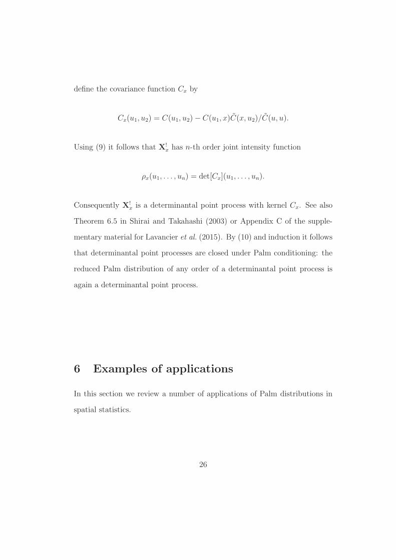
define the covariance function Cx by

Cx(u1, u2) = C(u1, u2)− C(u1, x)C(x, u2)/C(u, u).

Using (9) it follows that X!x has n-th order joint intensity function

ρx(u1, . . . , un) = det[Cx](u1, . . . , un).

Consequently X!x is a determinantal point process with kernel Cx. See also

Theorem 6.5 in Shirai and Takahashi (2003) or Appendix C of the supple-

mentary material for Lavancier et al. (2015). By (10) and induction it follows

that determinantal point processes are closed under Palm conditioning: the

reduced Palm distribution of any order of a determinantal point process is

again a determinantal point process.

6 Examples of applications

In this section we review a number of applications of Palm distributions in

spatial statistics.

26

Characteristic Poisson Gibbs

Density z−1S

∏

v∈x ρ(v) ∝ exp{

−∑

∅6=y⊆x Φ(y)}

f(x)

Papangelou cond. ρ(u) exp{

−∑

y⊆x∪{u}:u∈y Φ(y)}

intensity λ(u,x)

Joint intensity∏n

i=1 ρ(xi) Ef({x1, . . . , xn} ∪ Z)ρ(n)(x1, . . . , xn)

One-point Palm z−1S

∏

v∈x ρ(v) ∝ exp{

−∑

∅6=y⊆x∪{u} Φ(y)}

density fu(x)

One-point Palm ρ(u) Ef({u, v} ∪ Z)/Ef({v} ∪ Z)intensity ρv(u)

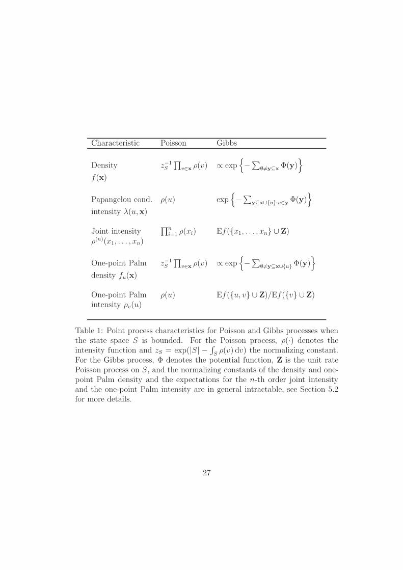
Table 1: Point process characteristics for Poisson and Gibbs processes whenthe state space S is bounded. For the Poisson process, ρ(·) denotes theintensity function and zS = exp(|S| −

∫

Sρ(v) dv) the normalizing constant.

For the Gibbs process, Φ denotes the potential function, Z is the unit ratePoisson process on S, and the normalizing constants of the density and one-point Palm density and the expectations for the n-th order joint intensityand the one-point Palm intensity are in general intractable, see Section 5.2for more details.

27

Characteristic Cox Determinantal

Density Ef(x | Λ) ∝ det[C](x)f(x)

Papangelou cond. Ef(x ∪ {u} | Λ)/Ef(x | Λ) det[C](x ∪ {u})/det[C](x)intensity λ(u,x)

Joint intensity E∏

v∈x Λ(v) det[C](x1, . . . , xn)ρ(n)(x1, . . . , xn)

One-point Palm Ef(x | Λu) ∝ det[Cu](x)density fu(x)

One-point Palmintensity ρv(u) E{Λ(u)Λ(v)}/EΛ(v) det[C](u, v)/C(v, v)

Table 2: Point process characteristics for Cox and determinantal point pro-cesses when the state space S is compact. For the Cox process, Λ denotes therandom intensity function, Λu is the modified random field (see Section 5.3),and f(·|Λ) is a Poisson process density when we condition on that Λ is theintensity function; all the expectations are in general intractable. For thedeterminantal point process, C denotes its kernel and we refer to Section 5.4for details on the related kernels C and Cu; the normalizing constants of thedensities are known (see Section 5.4).

28

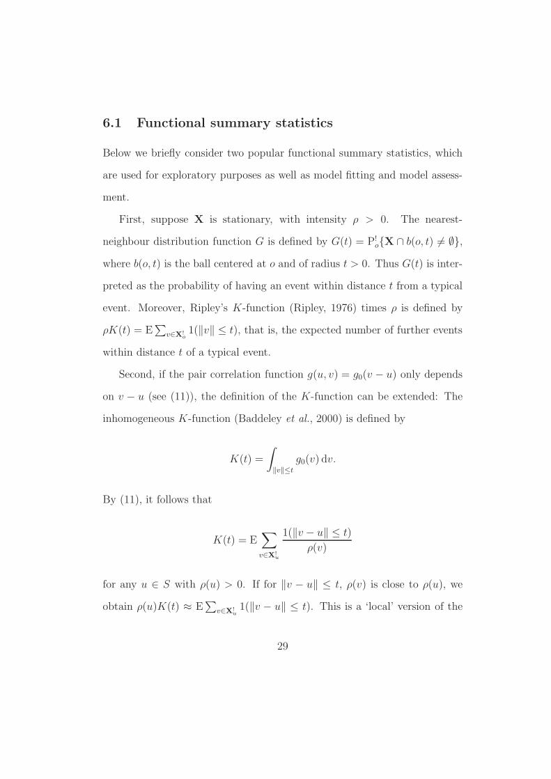
6.1 Functional summary statistics

Below we briefly consider two popular functional summary statistics, which

are used for exploratory purposes as well as model fitting and model assess-

ment.

First, suppose X is stationary, with intensity ρ > 0. The nearest-

neighbour distribution function G is defined by G(t) = P!o{X ∩ b(o, t) 6= ∅},

where b(o, t) is the ball centered at o and of radius t > 0. Thus G(t) is inter-

preted as the probability of having an event within distance t from a typical

event. Moreover, Ripley’s K-function (Ripley, 1976) times ρ is defined by

ρK(t) = E∑

v∈X!o

1(‖v‖ ≤ t), that is, the expected number of further events

within distance t of a typical event.

Second, if the pair correlation function g(u, v) = g0(v − u) only depends

on v − u (see (11)), the definition of the K-function can be extended: The

inhomogeneous K-function (Baddeley et al., 2000) is defined by

K(t) =

∫

‖v‖≤t

g0(v) dv.

By (11), it follows that

K(t) = E∑

v∈X!u

1(‖v − u‖ ≤ t)

ρ(v)

for any u ∈ S with ρ(u) > 0. If for ‖v − u‖ ≤ t, ρ(v) is close to ρ(u), we

obtain ρ(u)K(t) ≈ E∑

v∈X!u

1(‖v − u‖ ≤ t). This is a ‘local’ version of the

29

interpretation of K(t) in the stationary case.

Nonparametric estimation of K and G is based on empirical versions ob-

tained from (15). For some parametric Poisson and Cox process models, K

or G are expressible on closed form and may be compared with correspond-

ing nonparametric estimates when finding parameter estimates or assessing

a fitted model. See Møller and Waagepetersen (2007) and the references

therein.

6.2 Prediction given partial observation of a point pro-

cess

Suppose S is bounded and we observe a point process Y contained in a finite

point process X specified by some density f with respect to the unit rate

Poisson process Z. If B ⊂ S with |B| > 0 and Y = XB, then prediction

of XS\B given Y = y can be based on the conditional density fS\B(·|y)

introduced in Section 2.3. On the other hand, if we just know that y ⊆ X,

then it could be tempting to try to predict X \ y using X!y. This would

in general be incorrect. For instance, for an LGCP with positive covariance

function, the intensity of X!y can be much larger than the one of X, cf.

(22). Thus on average X!y ∪y would contain more events than X. The issue

here is that the reduced Palm distribution is concerned with the conditional

distribution of X conditional on that prespecified points fall in X. Hence the

sampling mechanism that leads from X to Y must be taken into account.

30

For instance, if the distribution of Y conditional on X = x is specified by

a probability density function p(·|x) (on the set of all subsets of x), then

by Proposition 1 in Baddeley et al. (2000), the marginal density of Y with

respect to Z is

g(y) = ρ(n)(y) exp(|S|)E{

p(y|X!y ∪ y)

}

,

where n = n(y) is the cardinality of y. Thus the conditional distribution of

X \ y given Y = y has density

f(x|y) = p(y|x ∪ y)f(x ∪ y) exp(|S|)/g(y)

with respect to Z.

6.3 Matern-thinned Cox processes

Some applications of spatial point processes require models that combine

clustering at a large scale with regularity at a local scale (Lavancier and

Møller, 2015). Andersen and Hahn (2015) study a class of so-called Matern

thinned Cox processes where (clustered) Cox processes are subjected to de-

pendent Matern type II thinning (Matern, 1986) that introduces regularity

in the resulting point processes. The intensity function and second-order

joint intensity of the Matern-thinned Cox process is expressed in terms of

univariate and bivariate inclusion probabilities which in turn are expressed

31

in terms of one- and two-point Palm probabilities for the underlying Cox

process extended with a uniformly distributed mark for each event. In case

of an underlying shot-noise Cox process, explicit expressions for the univari-

ate inclusion probabilities are obtained using the simple characterization of

one-point Palm distributions described in Section 5.3.2.

6.4 Palm likelihood

Minimum contrast estimators based on the K-function or the pair correlation

function or composite likelihood methods are standard methods to fit para-

metric models (see e.g. Jolivet, 1991; Guan, 2006; Møller and Waagepetersen,

2007; Waagepetersen and Guan, 2009; Biscio and Lavancier, 2015). Tanaka

et al. (2008) proposed an approach based on Palm intensities to fit parametric

stationary models, which is briefly presented below.

Given a parametric model g(u, v) = g0(v − u; θ) for the pair correlation

function of X and a location u ∈ S, the intensity function of X!u is ρu(v; θ) =

ρg0(v−u; θ) where ρ is the constant intensity ofX assumed here to be known.

Following Schoenberg (2005), the so-called log composite likelihood score

∑

v∈X!u∩b(u,R)

d

dθlog ρu(v; θ)−

∫

b(u,R)

ρu(v; θ) dv

forms an unbiased estimating function for θ, where R > 0 is a user-specified

tuning parameter. Usually X!u is not known. However, suppose that X

is observed on W ∈ B0 and in order to introduce a border correction let

32

W ⊖R = {u ∈ W |b(u,R) ⊆ W}. Then, by (15),

6=∑

u∈X∩W⊖R,v∈X∩b(u,R)

d

dθlog ρu(v; θ)−N(W ⊖ R)

∫

b(o,R)

ρo(v; θ) dv (24)

is an unbiased estimate of the above composite likelihood score times ρ|W ⊖

R|. Tanaka et al. (2008) coined the antiderivative of (24) the Palm likelihood.

Asymptotic properties of Palm likelihood parameter estimates are studied by

Prokesova and Jensen (2013) who also proposed the border correction applied

in (24).

7 Concluding remarks

The intention of this paper was to give a brief and non-technical introdu-

tion to Palm distributions for spatial point processes. For more extensive

treatments of the topic we refer to Cressie (1993), Baddeley (1999), Van

Lieshout (2000), Daley and Vere-Jones (2008), Chiu et al. (2013), and Spo-

darev (2013). We omitted the case of marked point processes for sake of

brevity. The theory of Palm distributions for marked point processes is fairly

similar to that for ordinary point processes. Accounts of Palm distributions

for marked point processes can be found in Chiu et al. (2013) and Heinrich

(2013), while summary statistics related to Palm distributions for marked

point processes are reviewed in Illian et al. (2008) and Baddeley (2010).

We finally note that consideration of space-time point processes (Diggle

33

and Gabriel, 2010) suggests yet another useful notion of conditioning on the

past. For a space-time point process, the conditional intensity for a time-

space point (t, x) usually refers to the conditional probability of observing an

event at spatial location x at time t given the history of the space-time point

process up to but not including time t. So this conditional intensity naturally

takes the time-ordering into account, while there is no natural ordering when

considering a spatial point process.

Acknowledgments

We thank the editor and two referees for detailed and constructive com-

ments that helped to improve the paper. J. Møller and R. Waagepetersen

are supported by the Danish Council for Independent Research — Natural

Sciences, grant 12-124675, ”Mathematical and Statistical Analysis of Spatial

Data”, and by the ”Centre for Stochastic Geometry and Advanced Bioimag-

ing”, funded by grant 8721 from the Villum Foundation. J.-F. Coeurjolly

is supported by ANR-11-LABX-0025 PERSYVAL-Lab (2011, project Ocu-

loNimbus).

References

Andersen, I. & Hahn, U. (2015). Matern thinned Cox point processes. Spatial

Statistics 15, 1–21.

34

Baddeley, A. & Nair, G. (2012). Fast approximation of the intensity of Gibbs

point processes. Electronic Journal of Statistics 6, 1155–1169.

Baddeley, A., Møller, J. & Waagepetersen, R. (2000). Non- and semi-

parametric estimation of interaction in inhomogeneous point patterns. Sta-

tistica Neerlandica 54, 329–350.

Baddeley, A. J. (1999). Crash course in stochastic geometry. In: Stochas-

tic Geometry: Likelihood and Computation (eds. O. E. Barndorff-Nielsen,

W. S. Kendall and M. N. M. van Lieshout), Monographs on Statistics

and Applied Probability 80, Chapman & Hall/CRC, Boca Raton, Florida,

141–172.

Baddeley, A. J. (2010). Multivariate and marked point processes. In: Hand-

book of Spatial Statistics (eds. A. Gelfand, P. Diggle, P. Guttorp and

M. Fuentes), Chapman & Hall/CRC Handbooks of Modern Statistical

Methods, Taylor & Francis, 371–402.

Biscio, C. & Lavancier, F. (2015). Contrast estimation for parametric station-

ary determinantal point processes. Submitted for publication. Available at

arXiv:1510.04222.

Chiu, S., Stoyan, D., Kendall, W. S. & Mecke, J. (2013). Stochastic Geometry

and Its Applications . Wiley, Chichester, 3rd edition.

Coeurjolly, J.-F., Møller, J. & Waagepetersen, R. (2015). Palm distributions

35

for log Gaussian Cox processes. Submitted for publication. Available at

arXiv:1506.04576.

Coles, P. & Jones, B. (1991). A lognormal model for the cosmological mass

distribution. Monthly Notices of the Royal Astronomical Society 248, 1–13.

Cressie, N. A. C. (1993). Statistics for Spatial Data. Wiley, New York, 2nd

edition.

Daley, D. & Vere-Jones, D. (2003). An Introduction to the Theory of Point

Processes, Volume I: Elementary Theory and Methods . Springer, New

York, 2nd edition.

Daley, D. & Vere-Jones, D. (2008). An Introduction to the Theory of Point

Processes, Volume II: General Theory and Structure. Springer, New York,

2nd edition.

Dereudre, D., Drouilhet, R. & Georgii, H.-O. (2012). Existence of Gibbsian

point processes with geometry-dependent interactions. Probability Theory

and Related Fields 153(3-4), 643–670.

Diggle, P. J. & Gabriel, E. (2010). Spatio-temporal point processes. In:

Handbook of Spatial Statistics (eds. A. Gelfand, P. Diggle, P. Guttorp

and M. Fuentes), Chapman & Hall/CRC Handbooks of Modern Statisti-

cal Methods, Taylor & Francis, 449–461.

Georgii, H.-O. (1976). Canonical and grand canonical Gibbs states for con-

tinuum systems. Communications in Mathematical Physics 48, 31–51.

36

Georgii, H.-O. (1988). Gibbs Measures and Phase Transition. Walter de

Gruyter, Berlin.

Guan, Y. (2006). A composite likelihood approach in fitting spatial point

process models. Journal of the American Statistical Association 101, 1502–

1512.

Heinrich, L. (2013). Asymptotic methods in statistics of random point pro-

cesses. In: Stochastic Geometry, Spatial Statistics and Random Fields:

Asymptotic Methods (ed. E. Spodarev), Springer, Berlin, Heidelberg, 115–

150.

Illian, J., Penttinen, A., Stoyan, H. & Stoyan, D. (2008). Statistical Analy-

sis and Modelling of Spatial Point Patterns . Statistics in Practice, Wiley,

Chichester.

Jagers, P. (1973). On Palm probabilities. Probability Theory and Related

Fields 26, 17–32.

Jolivet, E. (1991). Moment estimation for stationary point processes in Rd.

In: Spatial Statistics and Imaging (Brunswick, ME, 1988), volume 20 of

IMS Lecture Notes Monograph Series , Institute Mathematical Statistics,

Hayward, CA, 138–149.

Kelly, F. & Ripley, B. (1976). A note on Strauss’ model for clustering.

Biometrika 63, 357–360.

37

Last, G. (1990). Some remarks on conditional distributions for point pro-

cesses. Stochastic Processes and Their Applications 34, 121–135.

Lavancier, F. & Møller, J. (2015). Modelling aggregation on the large scale

and regularity on the small scale in spatial point pattern datasets. Research

Report 7 , Centre for Stochastic Geometry and Advanced Bioimaging, to

appear in Scandinavian Journal of Statistics.

Lavancier, F., Møller, J. & Rubak, E. (2015). Determinantal point process

models and statistical inference. Journal of the Royal Statistical Society:

Series B (Statistical Methodology) 77(4), 853–877.

van Lieshout, M. N. M. (2000). Markov Point Processes and Their Applica-

tions . Imperial College Press, London.

Matern, B. (1986). Spatial Variation. Number 36 in Lecture Notes in Statis-

tics, Springer-Verlag, Berlin.

Møller, J. (1989). Random tessellations in Rd. Advances in Applied Proba-

bility 21, 37–73.

Møller, J. (1994). Lectures on Random Voronoi Tessellations . Lecture Notes

in Statistics 87, Springer-Verlag, New York.

Møller, J. (2003). Shot noise Cox processes. Advances in Applied Probability

35, 614–640.

38

Møller, J. & Waagepetersen, R. (2004). Statistical Inference and Simulation

for Spatial Point Processes . Chapman and Hall/CRC, Boca Raton.

Møller, J. & Waagepetersen, R. P. (2007). Modern spatial point process mod-

elling and inference (with discussion). Scandinavian Journal of Statistics

34, 643–711.

Møller, J., Syversveen, A. & Waagepetersen, R. (1998). Log Gaussian Cox

processes. Scandinavian Journal of Statistics 25, 451–482.

Neyman, J. & Scott, E. L. (1958). Statistical approach to problems of cosmol-

ogy. Journal of the Royal Statistical Society: Series B (Statistical Method-

ology) 20, 1–43.

Nguyen, X. & Zessin, H. (1979). Integral and differential characterizations of

Gibbs processes. Mathematische Nachrichten 88, 105–115.

Palm, C. (1943). Intensitatsschwankungen im Fernsprechverkehr. Ericssons

Techniks 44, 1–189.

Prokesova, M. & Jensen, E. (2013). Asymptotic Palm likelihood theory for

stationary point processes. Annals of the Institute of Statistical Mathemat-

ics 65(2), 387–412.

Ripley, B. D. (1976). The second-order analysis of stationary point processes.

Journal of Applied Probability 13, 255–266.

39

Ruelle, D. (1969). Statistical Mechanics: Rigorous Results . W.A. Benjamin,

Reading, Massachusetts.

Schoenberg, F. (2005). Consistent parametric estimation of the intensity of

a spatial-temporal point process. Journal of Statistical Planning and In-

ference 128, 79–93.

Shirai, T. & Takahashi, Y. (2003). Random point fields associated with cer-

tain Fredholm determinants. I. Fermion, Poisson and boson point pro-

cesses. Journal of Functional Analysis 2, 414–463.

Spodarev, E., ed. (2013). Stochastic Geometry, Spatial Statistics and Random

Fields: Asymptotic Methods . Springer, Berlin, Heidelberg.

Strauss, D. (1975). A model for clustering. Biometrika 63, 467–475.

Tanaka, U., Ogata, Y. & Stoyan, D. (2008). Parameter estimation for

Neyman-Scott processes. Biometrical Journal 50, 43–57.

Waagepetersen, R. & Guan, Y. (2009). Two-step estimation for inhomo-

geneous spatial point processes. Journal of the Royal Statistical Society:

Series B (Statistical Methodology) 71, 685–702.

40