A TRIDENT SCHOLAR PROJECT REPORT

NO. 525

Machine Learning Enabled Prediction of Atmospheric Optical Turbulence From No-Reference Imaging

by

Midshipman 1/C Skyler P. Schork, USN

UNITED STATES NAVAL ACADEMY ANNAPOLIS, MARYLAND

USNA-1531-2

This document has been approved for public release and sale; its distribution is unlimited.

REPORT DOCUMENTATION PAGE Form Approved

OMB No. 0704-0188 Public reporting burden for this collection of information is estimated to average 1 hour per response, including the time for reviewing instructions, searching existing data sources, gathering and maintaining the data needed, and completing and reviewing this collection of information. Send comments regarding this burden estimate or any other aspect of this collection of information, including suggestions for reducing this burden to Department of Defense, Washington Headquarters Services, Directorate for Information Operations and Reports (0704-0188), 1215 Jefferson Davis Highway, Suite 1204, Arlington, VA 22202-4302. Respondents should be aware that notwithstanding any other provision of law, no person shall be subject to any penalty for failing to comply with a collection of information if it does not display a currently valid OMB control number. PLEASE DO NOT RETURN YOUR FORM TO THE ABOVE ADDRESS.

1. REPORT DATE (DD-MM-YYYY) 5-16-22

2. REPORT TYPE

3. DATES COVERED (From - To)

4. TITLE AND SUBTITLE

Machine Learning Enabled Prediction of Atmospheric Optical Turbulence From 5a. CONTRACT NUMBER

No-Reference Imaging 5b. GRANT NUMBER

5c. PROGRAM ELEMENT NUMBER

6. AUTHOR(S) Skyler P. Schork

5d. PROJECT NUMBER

5e. TASK NUMBER

5f. WORK UNIT NUMBER

7. PERFORMING ORGANIZATION NAME(S) AND ADDRESS(ES)

8. PERFORMING ORGANIZATION REPORT NUMBER

9. SPONSORING / MONITORING AGENCY NAME(S) AND ADDRESS(ES) 10. SPONSOR/MONITOR’S ACRONYM(S) U.S. Naval Academy Annapolis, MD 21402 11. SPONSOR/MONITOR’S REPORT NUMBER(S) Trident Scholar Report no. 525 (2022) 12. DISTRIBUTION / AVAILABILITY STATEMENT This document has been approved for public release; its distribution is UNLIMITED.

13. SUPPLEMENTARY NOTES

14. ABSTRACT Laser based communication and weapons systems are integral to maintaining the operational readiness and dominance of our Navy. Perhaps one of the most intransigent obstacles for such systems is the atmosphere. As the beams travel through the atmosphere there is loss of irradiance on target, beam spread, beam wander, and intensity fluctuations of the propagating laser beam. The refractive index structure parameter, C2

n, is a measure of the intensity of the optical turbulence along a path. If C2

n can be easily and efficiently determined in an operating environment, the prediction of laser performance will be greatly enhanced. The goal of this research is to use image quality features in combination with machine learning techniques to accurately predict the refractive index structure parameter, C2

n. The models of particular interest to this research are the Generalized Linear Model, the Bagged Decision Tree, the Boosted Decision Tree, as well as the Random Forest Model. While the quantity of available training data had a significant impact on model performance, the findings indicate that image quality can be used to assist in the prediction of C2

n, and that the machine learning models outperform the linear model.

15. SUBJECT TERMS optical turbulence, machine learning, near-maritime environment, no-reference imaging

16. SECURITY CLASSIFICATION OF:

17. LIMITATION OF ABSTRACT

18. NUMBER OF PAGES

19a. NAME OF RESPONSIBLE PERSON

a. REPORT b. ABSTRACT c. THIS PAGE 72 19b. TELEPHONE NUMBER (include area code)

Standard Form 298 (Rev. 8-98) Prescribed by ANSI Std. Z39.18

U.S.N.A. --- Trident Scholar project report; no. 525 (2022)

MACHINE LEARNING ENABLED PREDICTION OF ATMOSPHERIC OPTICALTURBULENCE FROM NO-REFERENCE IMAGING

by

Midshipman 1/C Skyler P. SchorkUnited States Naval Academy

Annapolis, Maryland

_________________________________________(signature)

Certification of Adviser(s) Approval

Associate Professor John BurkhardtMechanical Engineering Department

_________________________________________(signature)

___________________________(date)

Professor Cody J. BrownellMechanical Engineering Department

_________________________________________(signature)

___________________________(date)

Associate Professor Charles NelsonElectrical and Computer Engineering Department

_________________________________________(signature)

___________________________(date)

Acceptance for the Trident Scholar Committee

Professor Maria J. SchroederAssociate Director of Midshipman Research

_________________________________________(signature)

___________________________(date)

USNA-1531-2

1

Abstract Laser based communication and weapons systems are integral to maintaining the operational readiness and dominance of our Navy. Perhaps one of the most intransigent obstacles for such systems is the atmosphere. This is particularly true in the near-maritime environment. Atmospheric turbulence perturbs the propagation of laser beams as they are subject to fluctuations in the refractive index of air. As the beams travel through the atmosphere there is loss of irradiance on target, beam spread, beam wander, and intensity fluctuations of the propagating laser beam. The refractive index structure parameter, 2, is a measure of the intensity of the optical turbulence along a path. If 2 can be easily and efficiently determined in an operating environment, the prediction of laser performance will be greatly enhanced. The goal of this research is to use image quality features in combination with machine learning techniques to accurately predict the refractive index structure parameter, 2. In order to construct a machine learning model for the refractive index structure parameter, a series of image quality features were evaluated. Seven image quality features were selected, and have been applied to an image dataset of 34,000 individual exposures. This dataset, along with independently measured 2 values from a scintillometer as the supervised variable, were then used to train a variety of machine learning models. The models of particular interest to this research are the Generalized Linear Model, the Bagged Decision Tree, the Boosted Decision Tree, as well as the Random Forest Model. While the quantity of available training data had a significant impact on model performance, the findings indicate that image quality can be used to assist in the prediction of 2, and that the machine learning models outperform the linear model.

Keywords: optical turbulence, machine learning, near-maritime environment, and no-reference imaging

2

Table of Contents 1 Introduction................................................................................................................................4 2 Background.................................................................................................................................5

2.1 Candidate Features......................................................................................................10 2.1.1 Image Gradient Sharpness Feature..............................................................10 2.1.2 Miller-Buffington Image Sharpness Feature...............................................11 2.1.3 Entropy.........................................................................................................12 2.1.4 PIQE, NIQE, and BRISQUE.......................................................................12 2.1.5 Mean Intensity.............................................................................................13 2.1.6 Laplacian of Gaussian..................................................................................14 2.1.7 Sobel............................................................................................................15 2.1.8 Temporal Hour Weight................................................................................16

2.2 Determination of 2....................................................................................................17 3 Method of Investigation.............................................................................................................20

3.1 Imaging Platform Selection........................................................................................20 3.2 Imaging Location........................................................................................................20

3.3 Image Quality Assessment..........................................................................................23 4 Data Collection..........................................................................................................................25 4.1 Data Overview............................................................................................................25 4.2 Data Partitioning.........................................................................................................26 5 Modeling....................................................................................................................................32 5.1 Feature Performance...................................................................................................32 5.2 Stepwise General Linear Model..................................................................................33 5.3 Bagged Regression Trees............................................................................................38 5.4 Random Forest............................................................................................................39 5.5 Boosted Model............................................................................................................41 6 Discussion..................................................................................................................................45 6.1 Model Generalization..................................................................................................45 7 Conclusion.................................................................................................................................47 8 Acknowledgments.......................................................................................................................49 9 References..................................................................................................................................50 Appendices.....................................................................................................................................53 Appendix A: MATLAB Code for the Image Sharpness, Edge Moment, and Mean Intensity.....53 Appendix B: MATLAB Code for Image Quality Assessment Features.......................................54 Appendix C: MATLAB Code for the Feature Performance Matrix.............................................57 Appendix D: MATLAB Code for the Generalized Linear Model................................................59 Appendix E: MATLAB Code for the Bagged Regression Tree Model........................................63 Appendix F: MATLAB Code for the Random Forest Model.......................................................66 Appendix G: MATLAB Code for the Boosted Regression Tree Model Case 1..........................68

3

Appendix H: MATLAB Code for the Boosted Regression Tree Model Cases 2-6.....................70

4

1 Introduction The performance of lasers that travel through the atmosphere can be adversely affected by atmospheric conditions. These adverse effects are of critical importance to the Navy, which employs laser-based weapons and communication systems in a variety of environments. Specifically, the turbulent fluctuations of temperature and other parameters within the atmosphere affect the refractive index of the medium and serve to distort a propagating laser beam [1]. This distortion of the laser beam, called optical turbulence, results in loss of coherence, increased beam spread, beam wander, and scintillation [1]. The combined effect of these phenomena is reduction in light intensity on the target. The varying fluctuations in intensity on target adversely impacts laser-based systems by increasing the minimum time-on-target to achieve desired results and lost data transmission [1]. In the atmosphere, the refractive index structure parameter, 2, is used to measure the intensity of optical turbulence that a laser beam encounters. While there are existing models that estimate the intensity of optical turbulence, these models can break down at lower altitudes [3]. This is particularly true in the near-maritime environment [2,3,16,19,35]. This research focuses on the use of image quality features to predict the intensity of optical turbulence, 2. A focus on imaging is useful because of its applicability to the Naval environment, while also being generalizable to a wider array of problems where quantification of turbulence is needed but sophisticated instrumentation is unavailable. Imaging will lead to higher information density and an increased ability to capture turbulent effects that are unable to be captured on existing platforms. While a number of features were evaluated, of particular interest to this research was the concept of sharpness. Sharpness is a measure of detail captured in images [10]. Four image sharpness features were further investigated in this research. The four image quality assessment features for sharpness are the Image Gradient, the Miller-Buffington Image Sharpness that derives sharpness from the intensity of the images, as well as the Sobel and Laplacian of Gaussian features which derive sharpness from identifying the existence and strength of edges in the images [8,13,14,20,25,26]. The goal of this Trident project is to understand the importance of image quality assessment features in their prediction of the refractive index structure parameter 2, as well as to evaluate a variety of machine learning models for the prediction of 2 based on the identified important image quality features. Imaging took place between observation points across the Severn river in Annapolis, MD in combination with a data set of 2 measurements collected by a Scintec Scintillometer along the same path.

5

2 Background In order to quantify 2 from information obtained from an image data set, it is important to understand the different image distortions. Image dancing resulting from turbulence is called image jitter [2]. Jitter is the phenomenon in which objects appear to move randomly from frame to frame in a sequence of images. It occurs when the image rate is slow enough so that the turbulence has enough time to change between exposures. For very high image rates it is expected that jitter will be substantially reduced as the turbulence is effectively constant between frames. Jitter is the result of the wave-front tilting while propagating through a turbulent field. Wave-front tilt is characterized by the angle the incoming light makes with respect to its original incoming light path normal to the receiver. The degree to which the wave-front tilts is measured upon the wave striking the imaging system and is given the name angle-of-arrival (AOA) [4]. The tendency of the wave to tilt while propagating through a turbulent field is due to refraction. When a wave travels from one medium into another with a different refractive index, it will bend. Mathematically, this relationship is given by Snell’s Law, ( ) = ( ) (1) where n is the index of refraction and is the angle of incidence. Therefore, as the wave propagates from the first medium indicated by the subscript “1” into the second medium indicated by the subscript “2”, the AOA will depend on the refractive index of the second medium relative to that of the first medium [5]. The atmospheric phenomena that have the largest effect on optical wave propagation are absorption, scattering, and refractive-index fluctuations [6]. Absorption is the conversion of light into internal molecular energy and then into heat, and scattering is the redirection of light intensity from molecules or small particles [6]. The primary cause of refractive index fluctuations are temperature variations in the atmosphere which can be thought of as turbulent cells or eddies illustrated in Fig. 1.

Figure 1: The effect of refractive index on a laser propagating through turbulent eddies.

The reason a laser beam acts differently as it propagates through a turbulent environment is because each of these eddies has a different index of refraction. Therefore, as established in Eqn.

6

1, if each eddy has a different index of refraction, then the angle of arrival of the beam at the receiver will be different depending on the path the light ray took to the receiver. Refractive index fluctuations lead to beam wander, irradiance fluctuations, and beam spread [6]. Beam expansion reduces the power per unit area at the receiver, or irradiance, because the intensity of the light is now spread over a larger area. Beam wander is primarily the result of large-scale turbulent cells at the transmitter. As the beam encounters these large eddies closer to the transmitter, the entire beam is captured and randomly carried by the eddy resulting in a lower mean irradiance on target. Irradiance fluctuations are primarily the result of the laser beam interacting with smaller turbulent cells. As the beam encounters these smaller eddies, part of the beam refracts away from its original path and part of the beam passes through the eddy. The result of these interactions with the smaller eddies is constructive and destructive interference of the beam as it continues propagating towards the receiver. This interference results in varying intensity at the receiver. This loss of irradiance can require an increased engagement time and adjustment of engagement range for directed weapons applications and lost transmission for communication systems. Beam spread is the expansion of the beam’s cross section and is the result of the interaction of the light with the turbulent eddies. Ultimately, beam spread is the consequence of scintillation which results in a crinkled wavefront [6]. All three effects of refractive index fluctuations, beam spread, beam wander, and irradiance fluctuations are illustrated in Fig. 2.

(a) (b)

Figure 2: Laser beam propagating over the water at Wallops Island, VA, at a distance of (a) 5-km and (b) 20-km

Figure 2 shows two snapshots of a laser beam propagating over the water off the coast of Wallops Island, VA. Figure 2a shows the laser beam at about 5 km - notice the beam is tight, narrow, and well-formed across the beam front with the exception of the cut-outs (black line across the middle) where photodetectors were placed. Figure 2b shows the same laser beam but after the beam had propagated closer to 20 km - notice the beam is much broader and more irregular. The turbulence level or path averaged value was essentially the same for both images. They were both in relatively low to mid-range turbulence conditions taken one night in

7

September of 2009. The only difference was that the distance was quadrupled for the image shown on the right in Fig. 2b. The normalized variance of fluctuations in irradiance at a target due to conditions that a laser beam encounters on its path is known as scintillation. Scintillation index is given in Eqn. 2 [1]

=< > −< >

< >

(2)

where I is the irradiance (power per unit area) of the beam. Angled brackets indicate an ensemble average. Figure 3 illustrates optical power variations collected in one second, again from the Wallops Island, VA data. The power received at the detector dropped ~40 dBm almost instantaneously at time 17.9 seconds, demonstrating how rapidly the optical power on a detector from a laser beam can fluctuate in a coastal environment.

Figure 3: Power on detector of received laser beam propagating over the ocean in Wallops

Island, VA. For a plane wave, the normalized variance in irradiance, defined in Eqn. 2, is equal to the to the Rytov variance , [6] = 1.23 (3)

where k is the wavenumber ( = 2 / ), L is the distance between the receiver and the transmitter, and 2 is the refractive index structure parameter. The index of refraction structure parameter, 2, describes the intensity of optical turbulence. Optical turbulence, caused by variations in the refractive index of the air is primarily driven by turbulent fluctuations in temperature.

8

Similar to the Rytov variance, the fluctuations of a laser beam can also be described by the Log Amplitude Variance given by, = 0.124 . (4)

For a spherical wave, the effects of optical turbulence can also be described by the Fried Parameter, . As atmospheric turbulence perturbs the wavefronts of the laser beam, the Fried Parameter is the distance over which the phase of the wavefront remains constant [36]. The Fried Parameter is given by,

=38

/

(0.423 ) . (5)

The index of refraction structure parameter, 2, can be physically measured using a device called a scintillometer. A scintillometer functions by using a beam of light over a path of known length to directly measure the variance in irradiance at a receiver, similar to Eqn 2, and obtain the value for the index of refraction structure parameter, 2. An example of data collected from a scintillometer can be viewed in Fig. 4.

Figure 4: An example of 2 vs. time from the 890m scintillometer link at the U.S. Naval

Academy over a 12-day period. Figure 4 is a graph produced from sample scintillometer data collected via the scintillometer link (890m) across the Severn River in Annapolis, MD shown in Section 3.2. The graph is a capture of 12-days from midnight of December 22, 2020 through noon of January 3rd, 2021. As can be observed, the levels of 2 (vertical axis) vary with time throughout the course of the collection from approximately 10-16 m-⅔ to 10-12 m-⅔. To demonstrate the effect of optical turbulence on laser propagation, an analysis in MATLAB was performed. In the code, the diffraction-limited spot size, illustrated by the smaller of the two

9

red rings in Fig. 5, was calculated for an arbitrary aperture, wavelength, and distance to the target. The larger of these two red rings in Fig. 5 illustrates the effects of both turbulence and diffraction. The smaller the spot size, the higher and more concentrated the intensity on target which results in a lesser required time on target for engagement.

Figure 5: Normalized spot size with (outer ring) and without (inner ring) optical turbulence.

The purpose of this calculation was to illustrate the large increase in spot size when turbulence is included. Figure 6 is a plot of irradiance, I, vs. 2, where the irradiance was determined from the turbulent spot size. Since the spot size gets bigger with larger values of 2, and the laser power stays the same, the power per area, or irradiance, decreases with increasing 2.

Figure 6: Relative irradiance vs. 2 for a representative engagement scenario.

10

Figure 6 quantifies the effect of optical turbulence on a beam in terms of mean irradiance. As can be seen in the figure, for very low 2 values on the order of 10-16 m-2/3, the target received ~100% of the emitted irradiance on target. However, as observed in the figure, as turbulence was introduced into the environment, the irradiance received on target drastically decreased due to the increased beam spread until the target received ultimately 0% of the emitted irradiance at a turbulence value on the order of 10-12 m-2/3. An analysis of Fig. 5 and Fig. 6 support the conclusion that irradiance, or the power on target for an engagement scenario, decreases in an increasing 2 turbulent environment.

2.1 Candidate Features

In order to pull our desired information from our collected images and construct a machine learning model, the following no reference image features were evaluated.

2.1.1 Image Gradient Sharpness Feature The first feature that we focused on was image sharpness. One example of the sharpness of an image, Mag Grad, was calculated by computing the sum of the magnitude of the gradient of the intensity of pixels in an image, G, and dividing it by the number of pixels [20]. This calculation is given by, =

1+ , = , =

(6)

where G is the numerical gradient of the intensity of the image, I, and N is the number of pixels in the image. As an example, the normalized Image Gradient sharpness was calculated for both an original image shown below in Fig. 7a and one which was blurred to simulate turbulent effects shown in Fig. 7b.

11

(a) (b)

Figure 7: Original image (a), blurred image (b) used for the Image Gradient sharpness calculation.

The normalized Image Gradient sharpness of the original image shown in Fig. 7a was calculated to be 1, while the normalized sharpness of the blurred image shown in Fig. 7b was calculated to be 0.56. These calculations support the claim that as image blurring increased, the magnitude of the image gradient sharpness feature decreased. A review of the MATLAB code used to calculate the image sharpness can be found in Appendix A.

2.1.2 Miller-Buffington Image Sharpness Feature An additional image sharpness feature, the Miller-Buffington image sharpness feature, determines the quality of detail in the image. The Miller-Buffington image sharpness is degraded by a process known as image blurring, the result of the image passing through the atmosphere. Miller-Buffington sharpness, MB, is the greatest for a pristine or undistorted image [8]. The Miller-Buffington image sharpness is given by = ∑ ∑

(∑ ∑ ) (7)

where Amn is the pixel value at the location, m,n where M is the number of rows of pixels and N is the number of columns of pixels in the image[8]. As an example, the normalized Miller-Buffington sharpness was calculated for both the original image shown above in Fig. 7a and one which was blurred to simulate turbulent effects shown in Fig. 7b. The normalized Miller-Buffington sharpness of the original image shown in Fig. 7a was calculated to be 1, while the normalized sharpness of the blurred image shown in Fig. 7b was calculated to be 0.95. These

12

calculations support the claim that as image blurring increased, the Miller-Buffington image sharpness of the image decreased. A review of the MATLAB code used to calculate this image sharpness feature can be found in Appendix A. 2.1.3 Entropy The third feature under consideration was the entropy present in the image. Entropy is a function that measures disorder. The highest quality and least distorted images will have the lowest entropy. The Entropy of an image, E, is given by

= − ( ) (8)

where = ∑ ∑ [12]. As the quality of an image degrades, the value of Entropy, E,

will increase. 2.1.4 PIQE, NIQE, and BRISQUE The fourth, fifth, and sixth features of interest, PIQE, NIQE, and BRISQUE are no-reference image quality assessment features built into the MATLAB image processing toolbox. The first step for all three of these image quality assessment features is a pre-processing step to extract the Natural Scene Statistics (NSS) from the grayscale images [23]. The reason that NSS features are extracted from normalized images is that differences in intensity distributions between normal and distorted photos is more apparent once the images are normalized [38]. This normalization is achieved through local mean removal and divisive normalization. The image intensity, I, at pixel location m,n is transformed into luminance values, , through the normalization process given by,

( , ) =( , ) − ( , )

( , ) +

(9)

where ( , ) = ∑ ∑ , , ( . )=−=−

And ( , ) = ∑ ∑ , ( , ( , )− ( , ))2

=−=−

where w is a 2D circularly symmetric Gaussian weighting function with K=L=3 standard deviations, C is a constant to prevent division by zero, and m,n 1,2….M,N, where M,N are the height and width of the image respectively [23]. The PIQE feature, the Perception Based Image Quality Evaluator, is an image quality score based upon a perception-based image quality evaluator [22]. The PIQE algorithm utilizes block-wise distortion estimation in order to determine the PIQE score for an image. This is accomplished by computing the Mean Subtracted Contrast Normalized (MSCN) coefficient, or the luminance values, , given in Eqn. 9, for distorted blocks of pixels in the images in accordance with Venkatanath et al’s proposed algorithm [23]. MSCN coefficients are well-

13

referenced in the world of human vision science to calculate image quality. These coefficients are also utilized to determine whether a given block of pixels is considered uniform or spatially active. Additionally, the magnitude of the variance of the MSCN coefficients, , is then used to calculate PIQUE score by determining the number of spatially active blocks for a certain threshold criterion value. PIQUE is then given by,

=1

+ 1 ÷ ( + 1)

(10)

where are the number of spatially active blocks in the given image and 1 is a constant to prevent division by zero [23]. As mentioned above, the Natural Scene Statistics (NSS) are relevant to the computation of NIQE and BRISQUE as well. NIQE values are determined by computing NSS features from pixel blocks in an image, fitting this information into a Multivariate Gaussian Model (MVG) which is then compared to the naturally fit MVG. The NIQE index, D, is given by,

( 1, 2, 1 2) = ( 1 − 2)∑ 1 + ∑ 2

2

1

( 1 − 2) (11)

where 1, 2,∑ 1 ,∑ 2 are the mean vectors and covariance matrices for the natural MVG model (1) and the distorted image’s MVG model (2) [23]. In order to obtain the NIQE score, this NIQE index is then compared to a database of natural images [23]. Once the luminance values, , are determined for an image, the BRISQUE algorithm specifies pair-wise products of the MSCN images. These pairwise products are given by, ( , ) = ( , ) ( , + 1)

( , ) = ( , ) ( + 1, ) 1( , ) = ( , ) ( + 1, + 1) 1( , ) = ( , ) ( + 1, − 1).

(12)

Eqn. 12 above dictates the four orientations where H is the horizontal, V is the vertical, D1 is the left-diagonal, and D2 is the right-diagonal that are utilized to determine the pairwise product images [38]. These four product images as well as the original MSCN image given by, , are then used to create a feature vector [38]. From this feature vector, a Support Vector Machine (SVM) computes a BRISQUE quality score. 2.1.5 Mean Intensity The seventh feature of interest was the mean intensity of the images. Image intensity is equivalent to the average pixel value of a gray-scale image. These intensities range from 0 [black] to 255 [white]. When an image is loaded into MATLAB, the program automatically is programmed to save the pixel values in an array. In order to calculate the mean intensity of each

14

image, the images were first converted to gray scale, and then the average pixel intensity value of all pixels in each image was determined. As an example, the normalized mean intensity was calculated for both an original gray-scale image shown below in Fig. 8a and one which was blurred to simulate turbulent effects shown in Fig. 8b.

(a) (b)

Figure 8: Original image (a), blurred image (b) used for the mean image intensity calculation.

The normalized mean image intensity of the original image shown in Fig. 8a was calculated to be 0.978, while the normalized mean image intensity of the blurred image shown in Fig. 8b was calculated to be 1. These calculations support the claim that as image blurring increased, the mean image intensity in the image increased as well. A review of the MATLAB code used to calculate the mean image intensity can be found in Appendix A. 2.1.6 Laplacian of Gaussian The eighth feature of interest was the Laplacian of Gaussian measure. It is calculated by applying a Laplacian of Gaussian filter to an image and then by finding edges by searching for zero-crossings [25]. The Laplacian of an image is the sum of second order derivatives given by,

( , ) = + (13)

15

where I is the image pixel intensity at the location x,y. Since the Laplace is applied to images that contain discrete pixels rather than a continuous distribution, a discrete convolution kernel is used to approximate the second derivative measurement [26]. These kernels are sensitive to noise and therefore a Gaussian smoothing filter is applied prior to the Laplacian convolution kernel [26]. The Gaussian and Laplacian kernels are convoluted into one filter given by,

( , ) = − 11 − +

2( )/

(14)

where is the scale of the filter. However, similar to Eqn. 13, Eqn. 14 is continuous and is discretized with an approximation kernel dictated by the magnitude of . The kernel extracts features from the images by essentially sliding over the input image and performing element-wise multiplication and subsequently summing the results in a given block of pixels. The output of this kernel is a discrete approximation of the Laplacian of Gaussian filter described in Eqn. 14. 2.1.7 Sobel The ninth feature under consideration was the Sobel edge moment. The Sobel feature is an image sharpness feature. In order to calculate the Sobel edge moment in an image, an edge detector uses a discrete differentiation operator in order to approximate the image gradient. One such detector is the Sobel Edge Detector. The Sobel Edge Detector functions by calculating the differences in intensities among neighboring pixels in an image [13]. The Sobel Edge Detector algorithm works best when images are converted first to grayscale. The algorithm uses two 3x3 convolution kernels to calculate the gradient in the x and y direction as shown below [14].

(15)

A convolution kernel is a matrix consisting of weighted indexes. The kernels serve as the filter in the Sobel Edge Detector algorithm. These gradient approximations are combined to yield the variance of the gradient moment in the images M (Eqn. 16),

= ( ) + ) (16)

where and are the convolution kernels defined in Eqn. 15 and A is the intensity of the tested image pixel value at the m,n pixel location. As the quality of the image degraded and distortions increased, the value of the Sobel edge moment, M, decreased. This is because the Sobel edge moment is calculated based on the strength of the intensity of the pixel values. The Sobel edge moment feature was calculated for both the original image and the blurred image shown in Fig. 7. An illustration of this calculation can be viewed in Fig. 9.

16

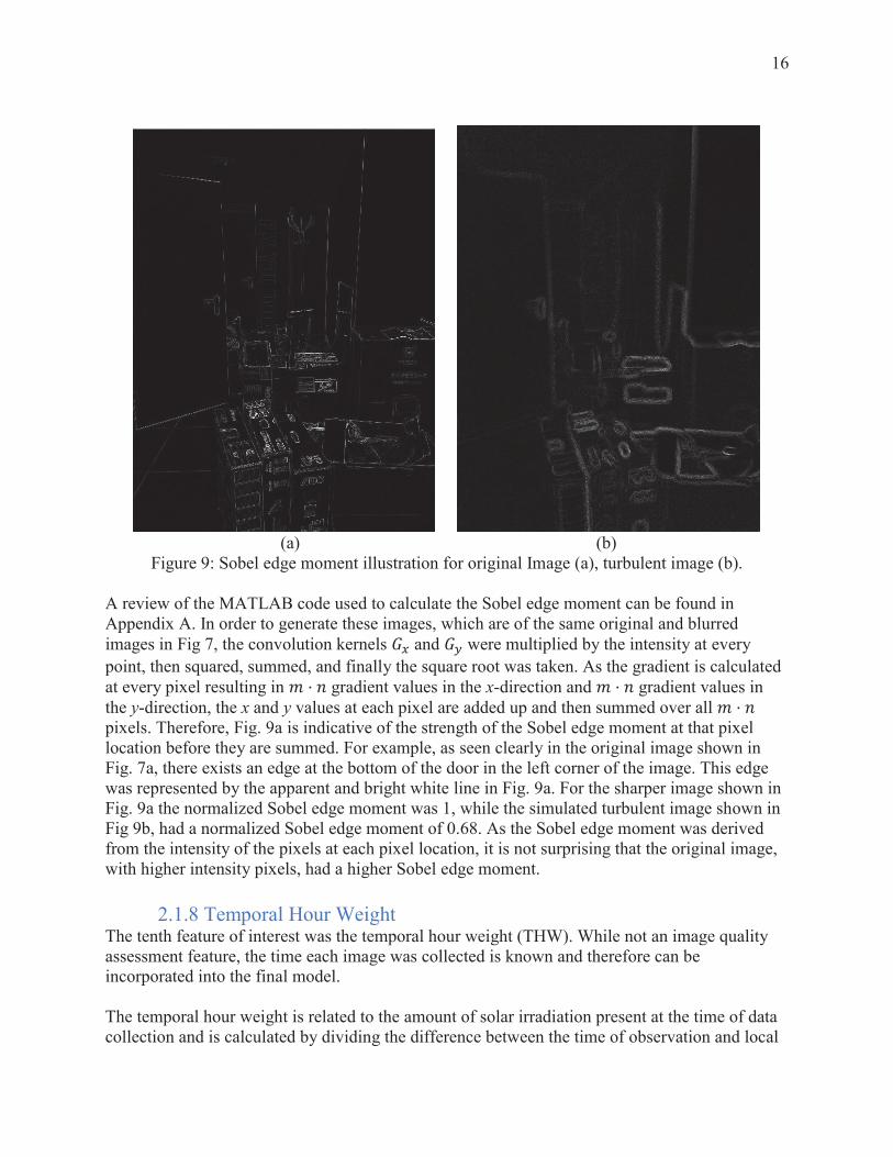
(a) (b)

Figure 9: Sobel edge moment illustration for original Image (a), turbulent image (b). A review of the MATLAB code used to calculate the Sobel edge moment can be found in Appendix A. In order to generate these images, which are of the same original and blurred images in Fig 7, the convolution kernels and were multiplied by the intensity at every point, then squared, summed, and finally the square root was taken. As the gradient is calculated at every pixel resulting in ⋅ gradient values in the x-direction and ⋅ gradient values in the y-direction, the x and y values at each pixel are added up and then summed over all ⋅ pixels. Therefore, Fig. 9a is indicative of the strength of the Sobel edge moment at that pixel location before they are summed. For example, as seen clearly in the original image shown in Fig. 7a, there exists an edge at the bottom of the door in the left corner of the image. This edge was represented by the apparent and bright white line in Fig. 9a. For the sharper image shown in Fig. 9a the normalized Sobel edge moment was 1, while the simulated turbulent image shown in Fig 9b, had a normalized Sobel edge moment of 0.68. As the Sobel edge moment was derived from the intensity of the pixels at each pixel location, it is not surprising that the original image, with higher intensity pixels, had a higher Sobel edge moment.

2.1.8 Temporal Hour Weight The tenth feature of interest was the temporal hour weight (THW). While not an image quality assessment feature, the time each image was collected is known and therefore can be incorporated into the final model. The temporal hour weight is related to the amount of solar irradiation present at the time of data collection and is calculated by dividing the difference between the time of observation and local

17

sunrise by 1/12 of the time between local sunrise and sunset [6]. The equation for temporal hour weight is shown below.

=12( − )−

(17)

Temporal hour weight has a value of 0 at sunrise and 12 at sunset.

2.2 Determination of 2 As discussed, 2, describes the intensity of optical turbulence. The determination of this structure parameter is twofold. With appropriate data, the thermo-fluid approach, targeting physical measurement is one method. This is juxtaposed by methods involving the analysis of the direct path of the light propagation. In this section, these two approaches are discussed as well as the importance of why it is critical that our model analyze the direct path of the light propagation, specifically in a one-sided manner.

One method to determine 2 experimentally is through the direct measurement of wind speed and temperature, often using a device called a sonic anemometer. Because these measurements are typically point-wise, the calculation typically assumes an atmospheric regime where optical turbulence behaves uniformly [19]. The temperature structure function can be calculated at this single point using a frozen turbulence hypothesis, and the structure constant can be extracted from the slope of the function. However, the equipment and techniques required for this approach are not standard, and therefore this remains a specialized approach. Alternatively, and perhaps more relevant to this line of research, is the analysis of the direct path of light propagation. The following is a description of two methods in which this is accomplished, the first is using a two-sided approach, and the second is using a one-sided approach. A two-sided approach is characterized by either a receiver and a transmitter or an imaging source and a target board collecting information about a turbulent environment. The receiver or imaging source is on one end and the target board is opposite the turbulent medium, hence the name two-sided. This two-sided approach is depicted in Fig. 10.

Figure 10: Two-sided analysis of the direct path of light propagation. A second example of a two-sided platform is the scintillometer. The scintillometer transmitter sends a light beam across a turbulent path. The characteristics of this source and the target receiver are both known, and therefore Eqn. 3 allows the scintillometer to calculate 2.

18

Conversely, a one-sided approach allows for only one instrument on one side of the turbulent environment to collect information. When employing a two-sided approach, the characteristics of the target board or imagining target are known. Therefore, when features are extrapolated and evaluated, there is a reference for comparison. However, moving into a one-sided analysis, the features of the imaging target are lost. While this allows for tremendous versatility in the imaging target, it is much harder to collect information across the field using this process. The one-sided approach is depicted in Fig. 11.

Figure 11: One-sided analysis of the direct path of light propagation.

The set-up in Fig. 11 is considered one-sided because there is only one instrument, the receiver, collecting information about the environment. For the purpose of this research the receiver used for this one-sided arrangement was a camera and the information collected of the environment were images. For the purpose of this research, a one-sided analysis of the direct path of light propagation is the method of interest. While the model is trained offline on a pre-existing selection of images, the images for analysis will be collected in real-time to allow the model to calculate turbulence values for the operating environment. Therefore, it is essential that the model is capable of evaluating images without known characteristics such as a target board. To our knowledge, while there exist commercial products to experimentally determine turbulence along a fixed path, there does not exist an alternative product for one-sided imaging. However, while a commercial model does not exist, a literature review has presented a number of researchers who have touched upon this approach [2,4,7]. Specifically, one approach proposed a method for 2 estimation given only an available recorded turbulence-degraded image sequence [2,7]. This method exploited the turbulence induced spatiotemporal movement across the frames of the image set in order to estimate the variance in angle-of-arrival obtained from different areas in the image [2,7]. The angle-of-arrival refers to the angle at which the laser reaches the receiver after being distorted by turbulence. This researcher used the variance in the angle-of-arrival in order to calculate values for 2. Another approach assessed a range of observable features in images due to the effects of turbulent air masses [4]. The features of interest were assessed along a horizontal path and then used to infer the strength of the turbulent air masses present in the atmosphere [4].

19

More recently, machine learning utilizing a decision tree and random forest model was employed in order to estimate 2 based on readily available atmospheric parameters [3]. This research found that machine learning was an effective method for improving atmospheric turbulence models, and identified the most important parameters to include in a model. The variables were time-averaged meteorological quantities (mean wind speed, air temperature, etc.) which do not have the same information density as images and which were not always proximate to the 2 measurements. For these reasons, in this study we are trying to extend the literature by using machine learning techniques in order to take the features from the images and train our model to accurately predict the 2 in the operating environment.

20

3 Method of Investigation 3.1 Imaging Platform Selection

In order to select an appropriate imaging system three distinct parameters were reviewed. These parameters included the aperture diameter, the distance to the target, and the exposure time. The camera originally proposed for this research was the B420 5MP Video Analytics Zoom Bullet Camera with D/N, Adaptive IR, Extreme WDR, SLLS, with a 36x Zoom Lens. In reviewing the work of other researchers in the field, it was determined that an assembly of the Canon EOS 5D Mark IV and Meade LX65 8” f/10 Optical tube would outperform the B420 camera [4]. Table 2 summaries the properties of these three imaging assemblies.

Table 2: The properties for the camera of interest

B420

Camera Canon EOS 5D Mark IV Camera with EF

70-200mm f/4L USM Lens Oerman’s

Assembly [4]

Aperture Diameter Range

106 mm 50 mm 200 mm

Focal Length 530 mm 200 mm 720 mm

Exposure Time 0.033

seconds 0.000125 seconds 0.2 seconds

In order for the camera to successfully capture the temporal fluctuations, the exposure time must be less than the correlation time, , which is given by the relationship [7], ≪ (18)

where V is the air speed in miles per hour. In the Annapolis area, the experimental environment, a typical air speed is around 1 m/s. The maximum aperture diameter (D) for the Canon EOS 5D Mark IV Camera is 50mm. For this experiment the L was the 890m across the Severn. With our aperture diameter of 0.05 m and an approximate air speed of 1 m/s, we yield an exposure time of 0.05 seconds. The Canon EOS 5D Mark IV camera, with a maximum shutter speed of 0.000125 seconds, therefore was able to reasonably capture weather conditions that fall within this range.

3.2 Imaging Location The operating environment of interest for this research includes an imaging path of 890m across the Severn River in Annapolis, MD. This operating environment was specifically selected due to the existing scintillometer link already installed across the Severn River. The scintillometer link across the Severn River from the Santee Basin to the Waterfront Readiness Center has been collecting data since 2019. On the left and right of Fig. 12 are the scintillometer receiver and

21

transmitter, and the orange dotted line depicts the 890m link across the Severn river over which the scintillometer is collecting 2 data.

Figure 12: Location of scintillometer link over the Severn River. The camera field of view will encompass this same over water path [3].

The Canon EOS 5D Mark IV Camera was initially paired with the Meade LX65 8” f/10 Optical tube for data collection, and this assembly was installed next to the scintillometer receiver located in the Santee Basin. The Canon-Optical tube assembly can be seen in Fig. 13a and 13b.

Figure 13: Initial experimental set-up; Canon EOS 5D Mark IV and Meade LX65 8” f/10 Optical

Tube.

While the intention of initially pairing the Canon EOS 5D Mark IV camera with the Optical Tube was to increase the focal length from 200mm to approximately 2000m, this new

22

experimental set-up introduced a serious flaw. A major problem that resulted in poor image quality was camera shake as a result of the shutter opening and closing to capture an image [28]. In order to overcome this problem, camera lenses to include the Canon EF 70-200mm f/4L USM Lens have a built-in optical image stabilizer system that utilizes a local microcomputer to counteract the shaking of the camera [28]. When the lens was removed from the experimental set-up and replaced with the Meade Optical Tube, without the integrated image stabilization system, the shutter produced considerable shake of the Optica Tube that was captured in the images. A photo taken with the Canon EOS 5D Mark IV and Meade LX65 8” f/10 Optical Tube assembly is shown in Fig. 14 below.

Figure 14: Image Taken Canon EOS 5D Mark IV and Meade LX65 8” f/10 Optical telescope.

This image was taken across the path illustrated in Fig. 12, and boxed in red is the Scintillometer transmitter. As can be seen in the figure, as a result of the camera shake originating from the opening and closing of the shutter and the lack of an image stabilization system integrated into the Optical Tube, the resulting photo is considerably blurry.

After this preliminary analysis of the data was performed it was concluded that it was necessary to prioritize the image stabilizing system over the increased focal length as many of the features of interest relate specifically to the sharpness of the images, and any increased image noise such as this blur would significantly inhibit the model’s ability to predict turbulence in the environment.

The revised experimentally set-up can be seen below in Fig. 15 consisting of the Canon EOS 5D Mark IV camera coupled with the Canon EF 70-200mm f/4L USM Lens.

23

Figure 15: Revised experimental set-up.

3.3 Image Quality Assessment In order to avoid time consuming and error-ridden subjective evaluation of images as performed by humans, image quality assessment has been at the forefront of digital media analysis in recent years [8]. This objective image quality assessment (IQA) is further partitioned into three variations to include full-reference (FR-IQA), reduced-referenced (RR-IQA), and no-reference (NR-IQA) image quality assessment.

Full-reference and reduced-reference image quality assessment rely on the existence of a reference image to which the test image can be compared. While these techniques produce excellent data, in many real-world applications, the reference image is typically not available for comparison. For instance, if a known object was repeatedly photographed and then this data was used to calculate the atmospheric turbulence, this would be an example of reduced reference image quality assessment. Specifically, this scenario is not full-reference because a pristine image of the known object was not obtained. However, while this works well when there is access to a sample known object, the goal of this Trident project is to enable operational commanders across the fleet to calculate the intensity of atmospheric turbulence, , when they do not have the same access to reference objects. Therefore, it is imperative that our model is trained on no-reference (NR-IQA) features. NR-IQA aims to quantitatively predict the quality of a distorted image using a computational model without the use of a reference image [8].

NR-IQA describes any number of techniques which attempt to assess the “quality” of an image without access to any prior information about the image. Images are subject to a wide variety of distortions due to both propagation through the atmosphere and processing during and after capture. Atmospheric effects, which are our focus, can be limited to blurring in both images and video and jitter in videos. Blurring in an image can be observed visually by studying the edge of

24

an object captured in a photograph. Blurring is the result of AOA fluctuations surrounding the edge under observation [4].

25

4 Data Collection 4.1 Data Overview As proposed by Oermann [4], it is estimated that 500 images are needed in an image sequence in order to deduce meaningful statistics from an image data set. Our preliminary test plan therefore was:

Time of Day Season Duration No. Images

AM-noon-PM Fall-Winter-Spring 1-hr >500 per set

This plan was, at minimum, 12 data collection sessions and 6000 images. In order to evaluate feature performance, the number of images captured during each session was increased considerably. The data set used in this research consisted of 34,446 images, the temporal equivalent of approximately 96 hours of data collection. This data collected spanned from January through April of 2022. Figure 16 is a histogram of the temporal hour weights recorded throughout the data collection.

Figure 16: Histogram of temporal hour weights recorded throughout data collection.

Temporal hour weight is a measure of the time that has passed since the sunrise relative to the sunset time for each day. A review of Fig. 16 shows that the data collection ranged from temporal hour weights of 0, associated with images collected right at sunrise, through 12,

26

associated with images collected right at sunset. To prevent error introduced into the data from images collected in low light, the data collection was restricted from sunrise to sunset. While it is evident that more data was collected at later times in the evening on average, all times of day were successfully captured in the data collection [4]. Figure 17 is a histogram of the 2 data collected throughout each data collection session.

Figure 17: Distribution of 2 values recorded by the scintillometer during the 96 hours of data

collection.

The distribution above at first glance appears seemingly normally distributed on a log scale. The log( 2) data plotted in Fig. 17 has a mean of -14.002, a standard deviation of 0.653, a median of -13.879, and a mode of -14.818. Since the median is slightly larger than the mean, the data is said to be positively skewed. Despite the slight skewness in the data, according to the literature

2 in the near maritime typically ranges from 10-16 to 10-12. Therefore, we can conclude that the sample of 2 values recorded throughout this data collection are representative of the location from which the data were pulled.

4.2 Data Partitioning In order to maximize the quantity of data that could be pulled from each individual photo as well as to expedite image processing time, each image that was collected was evaluated at five different regions of interest. These 5 regions were selected off of their image quality assessment suitability. These criteria included regions of the original image that consisted of strong and

27

defined edges, both horizontal and vertical features. Additionally, as these regions of interest were defined in an effort to increase the flexibility of the final model, it was important to select regions of interest that were at varying ranges from one another. Figure 18 below depicts a sample uncropped photo that has already been converted to grayscale with indicators as to each part of the photo that was further investigated.

Figure 18: Uncropped image highlighting all 6 regions of interest.

The regions of interest (RoI) highlighted above in Fig. 18 are discussed more thoroughly below in Table 5 to include an image description, the range from the camera to the region of interest, as well as a detailed picture of each region.

Table 5: Summary of regions of interest.

Region of Interest

Image Range

[m] Image Description Image of Region of Interest

A 890 Scintillometer

Receiver

28

B 770 Big Building Wall

C 1150 Small Building Wall

D 1180 Triangular Roof

E 1270 Base of Yacht

For each of the above regions of interest, satellite images were drawn from Google Maps to approximate the ranges listed above in Table 5. Figure 19 below includes all 5 satellite images from which the ranges were pulled.

(a) (b)

29

(c)

(d)

(e)

Figure 19: Google satellite images highlighted new ranges. Included in the figure are the ranges from the Santee Basin shown on the left of each image to regions of interest across the Severn

River: (a) the scintillometer transmitter, (b) the big building wall, (c) the small building wall, (d) the triangular roof, and (e) the base of yacht [39].

The data collected from the Google satellite images shown in Fig. 19 was used to scale images collected at different ranges. In order to account for the different ranges while constructing the models, 2 values were converted to both the Fried Parameter and separately to the Log Amplitude Variance. Given that 2 is computed as a path averaged value for a fixed distance, and given the above RoIs, each at different distances as shown in Fig. 19, we needed to consider a parameter other than 2 in order to account for the varying range while quantifying the turbulent intensity. To mitigate this, 2 values were converted to both the Fried Parameter and the Log Amplitude Variance, given in Eqns. 4 and 5, in order to obtain accurate metrics for each image, adjusted for range, from which the intensity of turbulent activity could later be derived. The MATLAB code used to process the data is included in Appendix B, and the experimental procedure by which data was extracted from the images is given below.

1. The camera was set to release shutter once every 10 seconds (6 photos/minute).

2. The scintillometer simultaneously recorded data.

3. The images were pulled from the camera and processed in MATLAB.

a. The images were converted to grayscale to give the intensity of the pixels across a

border spectrum and a smoothing filter was applied to prevent noise from

skewing feature calculations.

30

b. Each image was cropped to RoI A-E given in Table 5.

c. 7 features were calculated for each RoI.

i. Every six feature values were averaged together to yield one averaged

feature value per value of 2 (Table 6 below is an example of the data

averaging technique employed).

Table 6: Example of data averaging on a per minute basis.

Time Example Feature value Minute-Averaged

07:00:00 0.006787

1.46E-15

07:00:10 0.006526

07:00:20 0.006798

07:00:30 0.006983

07:00:40 0.006332

07:00:50 0.006787

*For time 07:00 the recorded feature value = 0.006702 for a 2 value of 1.46E-15

Once the averaged feature values were calculated for each of the 5 RoIs detailed in Table 5, the values were exported to an Excel spreadsheet that was later used to construct the machine learning models introduced in Section 5. The data that populated this Excel spreadsheet would later be partitioned between a training set and testing set in order to build the machine learning models. Table 7 below details 6 cases for which models were trained and how data was allocated for each scenario.

31

Table 7: Data partitioning scheme.

Training Set Testing Set

Case 1 Composed of 80% of all RoIs Composed of 20% of all RoIs

Case 2 Composed of 100% of RoIs

A,B,C,D Composed of 100% of RoI E

Case 3 Composed of 100% of RoIs A,B,C,E Composed of 100% of RoI D

Case 4 Composed of 100% of RoIs A,B,D,E Composed of 100% of RoI C

Case 5 Composed of 100% of RoIs A,C,D,E Composed of 100% of RoI B

Case 6 Composed of 100% of RoIs B,C,D,E Composed of 100% of RoI A

The six scenarios above dictate six different ways in which the data set was partitioned into training and test sets. In a regression tree analysis, the model uses the training set to fit initial trees. Once these trees are constructed, the model will use the test set to evaluate the model’s performance and accuracy in predicting the targeted response. Case 1 is entirely different from cases 2-6 because in this scenario the model is trained on every RoI and then tested on images that were selected from the same RoIs. This differs from cases 2-6 where the model was tested on RoIs it had never been trained on. Ideally, the model would perform similarly between all the cases.

32

5 Modeling Machine learning models are developed entirely from collected data and therefore allow the model to determine the significant parameters in the estimation of 2. This is in contrast to physical models which function by predetermining the effect of specific parameters. Machine learning models achieve this by allowing the model to observe the data and generate predictions based off of the data. The objective of machine learning is to generate predictions through application of repeated statistical models to the data set [16]. This process enlists the application of many statistical models on the data set in order to find patterns in very large sets of data. Machine learning is a favorable approach in the estimation of 2 because it offers the possibility of more accurate results. Additionally, machine learning expands the experimental design space as the techniques can be applied to extremely large data sets containing hundreds of different parameters. As discussed earlier, in order to accurately account for the varying ranges shown in Table 5, the models were trained on derived from both the Log Amplitude Variance as well as the Fried Parameter. The Log Amplitude Variance and the Fried Parameter were given in Eqns. 3 and 4. Broadly speaking, machine learning can be classified as either supervised or unsupervised [16]. With unsupervised machine learning, there is no supervising output for a given input. Conversely, a supervised learning model works by analyzing the relationship between the supervised output data with the collected input data in order to build a model for prediction and estimation [16]. For this research supervised learning was selected. Seven of the candidate image quality features previously discussed in Section 2.2 were selected for incorporation into the final modes. Additionally, two supervised data sets were evaluated for this research. These supervising data sets were the Fried Parameter and the Log Amplitude Variance. These values were calculated using Eqns. 4 and 5 from the scintillometer generated 2 data that was collected simultaneously to the imaging data set. The scintillometer generated 2 data is shown in Fig. 17. This is the supervised data or training data set that was used calculate the Fried Parameter and the Log Amplitude Variance which were then used to train the models. Machine learning models differentiate between classification and regression methods. For classification problems, the output is typically categorical or qualitative in nature, while for a regression problem, the output is numerical or quantitative in nature [16]. As the intent of this research is to predict a numerical value for 2, a regression analysis was required. Through the course of this research one supervised linear model and three supervised ensemble models were trained. The linear model of interest was the generalized linear model, while the tree ensemble models that were trained employed Bagging, Random Forest, and Boosting techniques. 5.1 Feature Performance Prior to the construction of the models, the suitability of the predictor features was examined to prevent a poor predictor feature from inhibiting the strength of the developed models. In order to determine the performance of each feature, a scatterplot matrix was created to demonstrate the relationship between each and every one of the other features to include itself. This scatterplot

33

matrix is shown in Fig. 20. The MATLAB code for this scatterplot matrix is included in Appendix C.

Figure 20: Scatter plot matrix for feature performance.

The main takeaway from the figure above is regarding the shape of each plot. A cluster, or random distribution is a positive result. If there were a relationship between the features so that there was some sort of trendline to follow, this would indicate that one of these features would not need to be included into the final model. This is because a relationship indicates that the features are correlated whereas a random distribution indicates that the features are uncorrelated and carry dissimilar information. The second main takeaway from Fig. 20 relates to the histograms that populate the diagonal of the figure as a result of the features being plotted against themselves. The three features that draw negative attention in Fig. 20 are the NIQE, Miller-Buffington Sharpness, and BRISQUE features. The reason these three features are identified is because an analysis of their respective histogram shows that these features have a tendency to populate one or two distinct values rather than assume a normal distribution. If these features were incorporated into the model this would be detrimental to its performance as a normal distribution of 2 values were collected. It is for these reasons that the NIQE, Miller-Buffington Sharpness, and BRISQUE features were not included when constructing the final models. 5.2 Stepwise Generalized Linear Model A stepwise regression is a specific kind of a multiple linear regression where terms are systematically added and removed from the model based on a certain criterion [30]. The reason that stepwise regression was selected for this analysis was due to the fact that there was significant uncertainty as to which, if any, features would hold the statistical significance in determining the response. The criterion that determines this is based on the statistical significance the term has in determining the response [30]. The criterion most commonly used in

34

literature for this situation is the mean square error (MSE). The MSE is used to quantify the performance of statistical learning models, and is a measure of the variation between the predicted response and true response value for a set of observations. The MSE is defined as the following,

=1

( − ( )) (19)

where the MSE is calculated by averaging the sum of the n observations of the squared difference between the model predicted value, , and the supervised value, . There are three components to a generalized linear model (GLM) to include a random component, a linear predictor, and a link function [29]. The random component specifies a response variable for 2 or the response variable as well as its distribution [29]. The linear predictor of the GLM includes a coefficient vector, = ( 1, 2, … ) , as well as an

× matrix, X, where n is the number rows for each observation, and p is the number of columns for each predictor variable. The linear predictor, , therefore is the product of the coefficient vector, , and the model matrix, X, and is given by = . The final component of the GLM, the link function, relates the random component and the linear predictor. The link function if given by,

( ) = , = 1, … (20)

where = ( ). Given the above model in Eqn. 20, when ( ) = , we call this the identity link function where = [29]. This is the case in an ordinary linear model that assumes the observations have a constant variance. A GLM differs from this because instead of equating the linear predictor directly to the mean of the response variable and assuming constant variance across the observations, the linear predictor is equated to a link-function-transformed mean of the response variable, y. Applied to this experimental dataset, the general linear model for the predicted value, , is given by,

= + (21)

where the image quality features are indexed by = {1, … 7}, and X is a matrix of the training data. In order to build the stepwise generalized linear model, MATLAB fit an initial linear model to the data using Eqn. 21. Once this initial model was built, MATLAB then referenced each predictor term to determine their significance in determining the response variable [30]. When

35

referencing these terms, if any of the terms was found to be significant with a p-value less than the entrance tolerance of 0.05, then this term was kept in the model [30]. Additionally, if any of the initial or added terms had p-values greater than the exit tolerance of 0.1, this term was removed [30]. This sequence was continued until the algorithm could identify the features that assumed the greatest significance in predicting the response [30]. For this research, two stepwise linear regression models were built. In the first model, interaction terms were not allowed. An interaction is defined as when one term has a different impact on the response depending on the value of the other terms [31]. When interaction terms are not allowed, there is one corresponding coefficient, j, per training feature, = {1, … 7}, in the X matrix. However, when interaction terms are allowed, a new coefficient, , is used to scale the new

interaction predictor value, = ⋅ . In order to train the GLM, 80% of the data collected was categorized as the training set, while the remaining 20% was used to test the model. The results of the first stepwise linear regression model for the prediction of the Fried Parameter are given in Table 8. Table 8: Results of stepwise generalized linear regression without interaction terms to predict the

Fried Parameter.

Feature Coefficient ( ) Estimate Square Error p-value

Intercept 0 -1.58 0.101 1.8810

Sobel 1 18.7 1.41 5.6010

PIQE 2 - - -

Mean 3 0.105 0.0520 0.0428

MG 4 -23.6 1.08 ~0

LoG 5 - - -

Entropy 6 0.327 0.0188 8.3510

THW 7 0.0899 0.00280 ~0

The PIQE and Laplacian of Gaussian features were identified as explanatory variables whose p-values exceeded the exit threshold of 0.1. For these reasons these explanatory variables were removed from the general linear model because the model determined that they inhibited the construction of the model rather than assisted it. From Table 8, the stepwise generalized linear model for the prediction of the Fried Parameter is given by, ≅ −1.58 + ( )18.7 + ( )0.105 − ( )23.6 − ( )0.327 − ( )0.0899. (22)

36

For the given test set, the predicted values from the generalized linear model were then converted back into 2 values. The resulting predicted 2 values calculated from the predicted Fried Parameter values are shown in Fig. 21. Shown in Fig. 21c are the results when interactions between the explanatory variables were not allowed, and Fig. 21d are the results when interactions between explanatory variables were allowed. The results of the second stepwise linear regression model for the prediction of the Log Amplitude Variance are given in Table 9. Table 9: Results of stepwise generalized linear regression without interaction terms to predict the

Log Amplitude Variance.

Feature Coefficient ( ) Estimate Square Error p-value

Intercept 0 -0.1595 0.010 1.88× 10

Sobel 1 1.88 0.142 5.60× 10

PIQE 2 - - -

Mean 3 0.0106 0.00520 0.0428

MG 4 -2.38 0.109 ~0

LoG 5 - - -

Entropy 6 0.0330 0.00190 8.35 × 10

THW 7 0.00910 2.87× 10 ~ 0

From Table 9, the second stepwise generalized linear model for the prediction of the Log Amplitude Variance is given by, ≅ −0.1595 + ( )1.88− ( )0.0106− ( )2.38 + ( )0.0330 + ( )0.00910. (23)

For the given test set, the predicted values from this generalized linear model were also then converted back into 2 values. The resulting predicted 2 values calculated from the predicted the Log Amplitude Variance values are also shown in Fig. 21. Shown in Fig. 21c are the results when interactions between the explanatory variables were not allowed, and Fig. 21d are the results when interactions between explanatory variables were allowed. The red line present in each of the four plots below is indicative of how a perfect model would perform whereby the predicted values would be equal to the measured values, building a perfectly straight 45-degree line. The script used to build this model can be reviewed in Appendix D.

37

(a)

(b)

(c)

(d)

Figure 21: (a) Stepwise generalized linear model for the Fried Parameter (no interaction terms), (b) Stepwise generalized linear model for the Fried Parameter (with interaction terms), (c)

Stepwise generalized linear model for the Log Amplitude Variance (no interaction terms), (d) Stepwise generalized linear model for the Log Amplitude Variance (with interaction terms)

Consistent with the literature [34,35], a review of Fig. 21 supports the conclusion that the generalized linear model failed to predict 2 for both cases when it was derived from the predicted Fried Parameter (Fig. 21(a)) and from when it was derived from the Log Amplitude Variance (Fig. 21(b)). The Mean Square error was calculated for each of the four models shown in Fig. 21 based off of the predicted 2 values and the given or measured 2 values. The Generalized Linear Model without interaction terms attained an MSE of 0.5677 both when 2 was derived from the Fried Parameter and the Log Amplitude Variance. The Generalized Linear Model with interaction terms attained an MSE of 0.6027 for both scenarios as well. While the model performed better when interaction terms were not allowed, the 0.035 improvement proves to be nominal and the main conclusion given the results in Fig. 21 is that a generalized linear model fails to predict the response variable. With that being said there was benefit modeling this linear approach to observe the evident nonlinear relationship between the predictor matrix and determined response.

38

5.3 Bagged Regression Trees

The Bagged Regression Tree was the next method that was evaluated for model performance in this research. Bagging is a technique used to mitigate variance within a dataset [32]. Bagging is a technique used where separate decision trees are created off of bootstrapped copies of original data, where the final model is a combination of all the separate decision trees [18]. Using the bootstrap technique, certain pockets of data are allocated to specific decision trees. This technique reduces variance among the trees by preventing the same splitting criterion at each nodal partition from dominating the decision matrix [18]. For a set of random observations, n,

the variance of the mean of the observations is given by, , where is the variance of the

observations. From this relationship it becomes clear that in order to reduce the variance, we can average a set of observations. This conclusion lends itself to the discussion of statistical learning where predicted models are averaged to reduce variance. However, it is typically impractical to collect enough training sets to be able to construct enough separate prediction models [18]. In order to mitigate this, a technique known as bootstrapping is often employed. Bootstrapping is a technique where multiple random samples are repeatedly drawn from the same single training data set. Bagging is the result of applying this bootstrapping technique to train a model [18]. The bagged model is given by,

( ) =1 ∗ ( )

=1

(24)

In order to apply bagging to a regression tree, a fixed number of trees, B, are constructed using a fixed number of random samples, b, from the training data set, and the resulting predictions are averaged. An initial Bagged Regression Tree was constructed using the same Case 1 data partitioning from Table 7 where 80% of the data collected was categorized as the training set, while the remaining 20% was used to test the model. For the given test set, the predicted Fried Parameter and Log Amplitude Variance values from these Bagged Regression Trees were then converted back into

2 values for analysis. The code for the Bagged Regression Tree is included in Appendix G and the model performance is shown in Fig. 22.

39

(a)

(b)

Figure 22: Bagged Regression Tree model trained on derived from predict Fried Parameter (a) and Log Amplitude Variance (b) for Case 1.

As shown in Fig. 22 an initial visual analysis suggests that the Bagged Regression Tree had a higher accuracy prediction rate as compared to the generalized linear models shown in Fig. 21. This preliminary analysis is supported by the mean square error of the Bagged Regression Tree model with a value of 0.1476 when trained for both the prediction of the Fried Parameter and the Log Amplitude Variance. This statistic is nearly 1/5 of that calculated for either generalized linear model when trained for the prediction of the Fried Parameter.

5.4 Random Forest Random Forests historically are known to outperform Bagged trees by decorrelating the trees utilized by the model [18]. The process of building multiple trees trained on bootstrapped training samples is the same as in Bagging, however now, each time a split is considered in the tree, the split is selected based on a random sample of predictors. For a sample size of p predictors, a random sample of m predictors is selected. The standard practice is to take ≈ . The reason why Random Forest models are forced to select such a small random sample of predictors is to prevent one strong predictor in the data set from dominating the formation of the trees. In bagging, a strong predictor has the potential to drive the construction of all of the trees since this random sample is not allocated, and as a result many of the trees end up with stark similarities. Random Forest models use this random sample in order to decorrelate trees as on average ( − )/ of the potential splits in the random sample do not include the strongest identified predictor. Ultimately the Random Forest model differs from the Bagged Regression Tree in regards to the size of m. When Bagging is employed, all of the predictors are considered at the nodal partition. Mathematically this is the equivalent of stating that in Bagging the number of predictors considered, m, was equal to the total number of predictors, p. In a Random Forest model, m, is a random sample taken from p, and ≈ , in and in Bagging, = . The code for the Random Forest models is included in Appendix F, and the results for the Case 1 Random Forest models are shown below in Fig. 24. For the given test set, the predicted Fried Parameter and Log Amplitude Variance values from these Random Forest Models were converted back into

2 values for analysis.

40

(a)

(b)

Figure 23: Random Forest model trained on derived from the Fried Parameter (a) and Log Amplitude Variance (b) for Case 1.

As shown in Fig. 23 an initial visual analysis suggests that the Random Forest Model performed similarly to the Bagged Regression Tree shown in Fig. 22, while highly outperforming the generalized linear models shown in Fig. 21. This preliminary analysis is supported by the mean square error of the Random Forest model with a value of 0.1686 when trained for the prediction of the Fried Parameter as compared to the 0.5677 MSE by the generalized linear model with interaction terms trained for the prediction of the Fried Parameter. The MSE for the Random Forest models are significantly lower than that obtained by the generalized linear model with interaction terms for both the Fried Parameter and the Log Amplitude Variance. However, the MSE for the Random Forest model is approximately 13.3% higher than that obtained by the Bagged Regression Tree model. Figure 24 below shows the predictor importance plot for the Bagged Regression Tree on the left, and the predictor importance plot for the Random Forest model on the right.

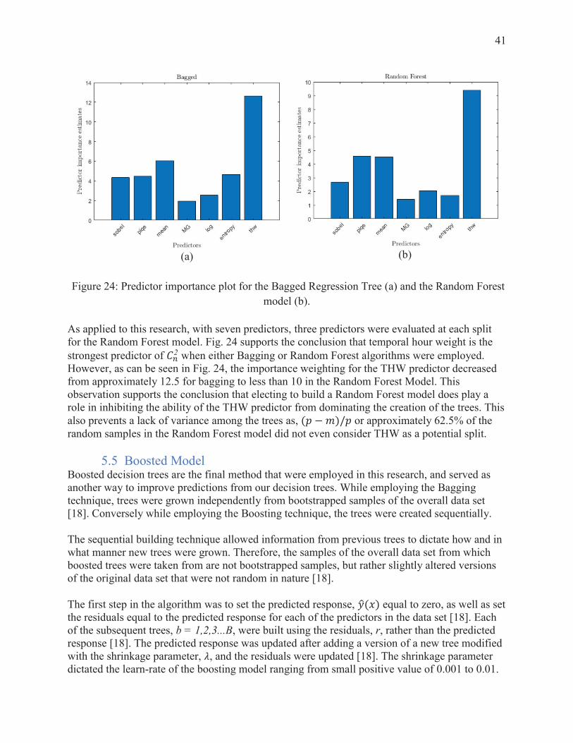
41

(a)

(b)

Figure 24: Predictor importance plot for the Bagged Regression Tree (a) and the Random Forest model (b).

As applied to this research, with seven predictors, three predictors were evaluated at each split for the Random Forest model. Fig. 24 supports the conclusion that temporal hour weight is the strongest predictor of 2 when either Bagging or Random Forest algorithms were employed. However, as can be seen in Fig. 24, the importance weighting for the THW predictor decreased from approximately 12.5 for bagging to less than 10 in the Random Forest Model. This observation supports the conclusion that electing to build a Random Forest model does play a role in inhibiting the ability of the THW predictor from dominating the creation of the trees. This also prevents a lack of variance among the trees as, ( − )/ or approximately 62.5% of the random samples in the Random Forest model did not even consider THW as a potential split. 5.5 Boosted Model Boosted decision trees are the final method that were employed in this research, and served as another way to improve predictions from our decision trees. While employing the Bagging technique, trees were grown independently from bootstrapped samples of the overall data set [18]. Conversely while employing the Boosting technique, the trees were created sequentially. The sequential building technique allowed information from previous trees to dictate how and in what manner new trees were grown. Therefore, the samples of the overall data set from which boosted trees were taken from are not bootstrapped samples, but rather slightly altered versions of the original data set that were not random in nature [18]. The first step in the algorithm was to set the predicted response, ( ) equal to zero, as well as set the residuals equal to the predicted response for each of the predictors in the data set [18]. Each of the subsequent trees, b = 1,2,3...B, were built using the residuals, r, rather than the predicted response [18]. The predicted response was updated after adding a version of a new tree modified with the shrinkage parameter, , and the residuals were updated [18]. The shrinkage parameter dictated the learn-rate of the boosting model ranging from small positive value of 0.001 to 0.01.

42

The literature suggests that the learning rate and the number of trees are inversely related such that a small learning rate may require a larger number of trees to improve accuracy [3]. The code for the Boosted regression tree models is included in Appendix H, and the results for the Case 1 Boosted regression models are shown below in Fig. 25.

(a)

(b)

Figure 25: Boosted regression tree model trained on derived from the Fried Parameter (a) and Log Amplitude Variance (b) for Case 1.

The Boosted regression tree performed well when compared to both the Bagged Regression Tree and the Random Forest model, while also outperforming the generalized linear models shown in Fig. 21. This preliminary analysis is supported by the mean square error of the Boosted regression tree model with a value of 0.1344 when trained on derived from the Fried Parameter. Additionally, the mean square error of the Boosted regression tree model had a value of 0.1343 when trained on derived from the Log Amplitude Variance. The mean squared errors achieved by the Boosted regression tree model were the smallest out of all of the models tested for both the Fried Parameter and the Log Amplitude Variance. In order to further evaluate the model. The Boosted regression tree trained on derived from the Log Amplitude Variance was evaluated for cases 2-6 as described in Table 7. The results of these tests are shown in Fig. 27 below. The analysis shown below illustrates the model’s accuracy in determining 2 values calculated from the model’s predictions for the Fried Parameter and the Log Amplitude Variance.

43

Case 2 - MSE 1.49

(a)

Case 3 - MSE 1.14

(b)

Case 4 - MSE 1.02

(c)

Case 5 - MSE 0.637

(d)

Case 6 – MSE 1.23

(e)

Figure 26: Cases 2-6 evaluated for the Boosted regression tree model.

44

A review of Fig. 26 ultimately shows that even the previously-established best performing model, the Boosted regression tree model, failed to predict accurate values for the Log Amplitude Variance for cases 2-6 where the model was tested on RoIs it had never seen before.

45

6 Discussion 6.1 Model Generalization As stated, the most successful model for the Case 1 scenario, where 80% of all the data consisting of all 5 RoIs was used to train the model, and the remaining 20% of all of the data was used to test the model, was the Boosted regression tree model. Using this model, Cases 2-6 were evaluated testing the model's ability to predict values for Log Amplitude Variance for RoIs it had never seen before. The code for these tests is included in Appendix H, and the results of these tests were discussed above in Fig. 27.

Table 9 below includes a summary of the mean square errors achieved by all of the models evaluated throughout the course of this research.

Table 9: Summary of mean square error for each of the regression trees modeled.

Trained Model Case 1

Trained on Fried Parameter

Trained on Log Amplitude Variance

Generalized Linear w/ Interaction Terms

0.6027 0.6027

Generalized Linear w/o Interaction Terms

0.5677 0.5677

Regression Tree

Bagged 0.1476 0.1467

Random Forest

0.1686 0.1667

Boosted 0.1344 0.1343

The success of the models shown above for the Case 1 scenario, was juxtaposed with the performance of the models when trained in accordance with the Case 2-6 scenarios. As shown in Fig. 27, when the model was asked to predict values for the Log Amplitude Variance from RoIs it had never been trained on before, the model ultimately failed. This suggests that a more thorough data collection is warranted.

The following is a discussion that supports the previous claim regarding whether or not the model can generalize. The following analysis was tested on the best-performing model, the Boosted regression tree model when trained on derived from the Log Amplitude Variance. To begin the analysis, the Boosted regression tree was trained only on the first RoI and tested on the second. This initial evaluation resulted in an MSE of 0.00944. Next, the model was trained on the second and third RoIs and tested on the first. The resultant MSE for this test was 0.0109. Thirdly, the model was trained on the RoIs 2-4, and tested on the first RoI for which the MSE

46

was 0.0128. And lastly, the model was trained on the RoIs 2-5, and tested on the first (identical to the Case 2 test) for which the MSE was 0.0107.

Ideally, as the models were trained on more RoIs, the resulting MSE would have dropped. Figure 27 is a visual illustration of the effect that testing on more RoIs had on the MSE.

Figure 27: Visual representation of the effect of testing on more RoIs had on the MSE of the predicted response.

A review of the information presented shows that training the model on more RoIs, with the intention of training the model to identify how the image quality features respond in different regions of the image, did not reduce the mean square error as expected. Instead, the MSE rose when the second and third RoIs were introduced, and then ultimately fell back down to an MSE of 0.0107 when four RoIs were used to train the model. This supports the conclusion that the model failed to generalize its results. While the model performed very well when tested on the RoIs it was trained on, the model failed to generalize across RoIs to be able to have the same results for Cases 2-6. Collecting more data, and potentially introducing more RoIs will help the model be able to generalize its results and ultimately improve the results generated when testing Cases 2-6.

0.00944

0.0109

0.0128

0.0107 009

0 010.01

TR

AIN

ON

2 R

OI

.01

010010

MS

E

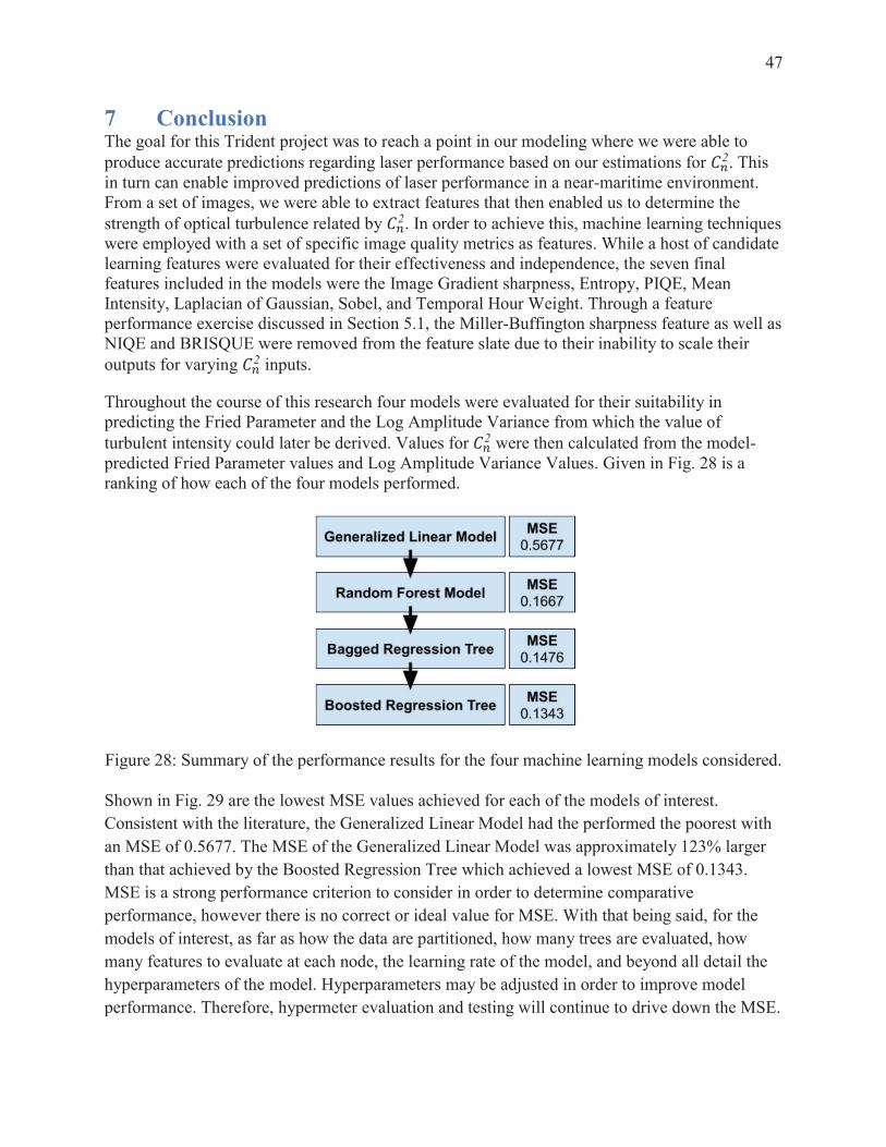
47

7 Conclusion The goal for this Trident project was to reach a point in our modeling where we were able to produce accurate predictions regarding laser performance based on our estimations for 2. This in turn can enable improved predictions of laser performance in a near-maritime environment. From a set of images, we were able to extract features that then enabled us to determine the strength of optical turbulence related by 2. In order to achieve this, machine learning techniques were employed with a set of specific image quality metrics as features. While a host of candidate learning features were evaluated for their effectiveness and independence, the seven final features included in the models were the Image Gradient sharpness, Entropy, PIQE, Mean Intensity, Laplacian of Gaussian, Sobel, and Temporal Hour Weight. Through a feature performance exercise discussed in Section 5.1, the Miller-Buffington sharpness feature as well as NIQE and BRISQUE were removed from the feature slate due to their inability to scale their outputs for varying 2 inputs.

Throughout the course of this research four models were evaluated for their suitability in predicting the Fried Parameter and the Log Amplitude Variance from which the value of turbulent intensity could later be derived. Values for 2 were then calculated from the model-predicted Fried Parameter values and Log Amplitude Variance Values. Given in Fig. 28 is a ranking of how each of the four models performed.

Figure 28: Summary of the performance results for the four machine learning models considered.

Shown in Fig. 29 are the lowest MSE values achieved for each of the models of interest. Consistent with the literature, the Generalized Linear Model had the performed the poorest with an MSE of 0.5677. The MSE of the Generalized Linear Model was approximately 123% larger than that achieved by the Boosted Regression Tree which achieved a lowest MSE of 0.1343. MSE is a strong performance criterion to consider in order to determine comparative performance, however there is no correct or ideal value for MSE. With that being said, for the models of interest, as far as how the data are partitioned, how many trees are evaluated, how many features to evaluate at each node, the learning rate of the model, and beyond all detail the hyperparameters of the model. Hyperparameters may be adjusted in order to improve model performance. Therefore, hypermeter evaluation and testing will continue to drive down the MSE.

48

The success of the Case 1 structured models was juxtaposed with the performance of the Case 2-6 structured models shown in Fig. 27. The lowest MSE achieved by one of the Boosted Regression Models in Fig. 27 was that for Case 5 which had an MSE of 0.637. Of note, however, this lowest MSE actually performed worse than the Generalized Linear Model. This analysis demonstrated the lack of generalization exhibited by the models. In order to combat this lack of generalization future work includes collecting more data and including more RoIs. This inability to effectively generalize supports the conclusion that the model performs extremely well when fed images of features it has seen before, however it struggles when unknown images are presented. Therefore, future work will also include training the models on features most likely to be present in near-maritime operating environments such as bridges and buildings in higher resolution than was achieved in our research in order to assist the model in predictions.

In conclusion, the goal of this Trident project was to assess feature importance in determining the refractive index structure parameter 2, as well as to build a machine learning model for the

prediction of 2. The Boosted Regression Tree with an MSE of 0.1343 which utilized the Image Sharpness Gradient, the Entropy, the PIQE, the Mean Intensity, the Sobel and Laplacian of Gaussian Measures, as well as the Temporal Hour Weight of each of the collected images to predict 2 successfully met these identified objectives for the Case 1 data partitioning.

49

8 Acknowledgments This work could not have been accomplished without the unwavering support and advice of Professor John Burkhardt, Professor Cody Brownell, and Professor Charles Nelson. Further instruction and review from Christopher Jellen and Professor Ethan Lust, were key throughout the research process. I would also like to acknowledge my classmates Zane Buono and Xavier Coburn who demonstrated tremendous support throughout this research as well by assisting in the data collection process. The authors would also like to thank the United States Naval Academy Mechanical Engineering and Electrical Engineering Departments for their assistance in data collection, model critique, and editorial review. Finally, we would like to thank the Trident Committee and Professor Maria Schroeder for their generous support.

50

9 References

1. Jensen, Douglas R., Stuart G. Gathman, Carl R. Zeisse, Charles P. McGrath, Gerrit de Leeuw, Michael A. Smith, Paul A. Frederickson, and Kenneth L. Davidson. "Electro-optical propagation assessment in coastal environments (EOPACE): summary and accomplishments." Optical Engineering 40, no. 8 (2001): 1486-1498.

2. Zamek, Sharon. Turbulence Estimation from a Set of Atmospherically Degraded Images and Application to Image Correction. Ben-Gurion University of the Negev, 2006.

3. Jellen, Christopher, John Burkhardt, Cody Brownell, and Charles Nelson. "Machine learning informed predictor importance measures of environmental parameters in maritime optical turbulence." Applied Optics 59, no. 21 (2020): 6379-6389.

4. Oermann, Raymond James. "Novel methods for the quantification of atmospheric turbulence strength in the atmospheric surface layer." PhD diss., 2014.

5. Hecht, E. (2016). Optics (5th ed.). Boston: Pearson. 6. R. Andrews, L.C. & Phillips, Laser Beam Propagation through Random Media.

Bellingham: SPIE Press, 2nd ed., 2005. 7. Zamek, Steve, and Yitzhak Yitzhaky. "Turbulence strength estimation from an arbitrary

set of atmospherically degraded images." JOSA A 23, no. 12 (2006): 3106-3113. 8. Xu, Shaoping, Shunliang Jiang, and Weidong Min. "No-reference/blind image quality

assessment: a survey." IETE Technical Review 34, no. 3 (2017): 223-245. 9. Espinola, Richard L., Jae Cha, and Kevin Leonard. "Novel methodologies for the

measurement of atmospheric turbulence effects." In Infrared Imaging Systems: Design, Analysis, Modeling, and Testing XXI, vol. 7662, p. 76620W. International Society for Optics and Photonics, 2010.

10. Sharpness: What is it and how is it measured? (n.d.). Retrieved January 16, 2021, from https://www.imatest.com/support/docs/pre-5-2/sharpness/

11. Muller, Richard A., and Andrew Buffington. "Real-time correction of atmospherically degraded telescope images through image sharpening." JOSA 64, no. 9 (1974): 1200-1210.

12. Rios, Carlos, and Szymon Gladysz. "No-reference image quality assessment for horizontal-path imaging scenarios." In Photonic Applications for Aerospace, Commercial, and Harsh Environments IV, vol. 8720, p. 872006. International Society for Optics and Photonics, 2013.

13. An Implementation of Sobel Edge Detection. (n.d.). Retrieved January 16, 2021, from https://www.projectrhea.org/rhea/index.php/An_Implementation_of_Sobel_Edge_Detection

14. Sobel Edge Detector. (n.d.). Retrieved January 16, 2021, from https://homepages.inf.ed.ac.uk/rbf/HIPR2/sobel.htm

15. L. Andrews, R. Phillips, and C. Hopen, Laser Beam Scintillation with Applications. Bellingham, Washington, USA: SPIE Press, 1ed. 2001. 201.

51

16. Raj, A. A. B., Selvi, J. A. V., & Durairaj, S. (2015). Comparison of different models for ground-level atmospheric turbulence strength (Cn 2) prediction with a new model according to local weather data for FSO applications. Applied optics, 54(4), 802-815.

17. Sadot, D., & Kopeika, N. S. (1992). Forecasting optical turbulence strength on the basis of macroscale meteorology and aerosols: models and validation. Optical Engineering, 31(2), 200-213.

18. James, G., Witten, D., Hastie, T., & Tibshirani, R. (2017). An Introduction to Statistical Learning with Applications in R. New York, NY: Springer.

19. Tunick, A. D. (1998). The refractive index structure parameter/atmospheric optical turbulence mode: CN2 (No. ARL-TR-1615). ARMY RESEARCH LABORATORY ADELPHI MD.

20. Birdal, Tolga (2010). Sharpness Estimation From Image Gradients (https://www.mathworks.com/matlabcentral/fileexchange/32397-sharpness-estimation-from-image-gradients), MATLAB Central File Exchange. Retrieved December 1, 2021.

21. "Two-sample t test for difference of means" (video). Khan Academy. Accessed December 1, 2021. https://www.khanacademy.org/math/ap-statistics/xfb5d8e68:inference-quant itative-means/two-sample-t-test-means/v/two-sample-t-test-for-difference-of-means.

22. Sheikh, H. R., Z. Wang, L. Cormack and A.C. Bovik. LIVE Image Quality Assessment Database Release 2, https://live.ece.utexas.edu/research/quality/.

23. Venkatanath N., Praneeth D., Maruthi Chandrasekhar Bh, Sumohana S. Channappayya, and Swarup S. Meda. Blind Image Quality Evaluation Using Perception Based Features. Department of Electrical Engineering, Indian Institute of Technology Hyderabad.

24. Raj, Ashwin. Unlocking the True Power of Support Vector Regression. Towards Data Science. Published October 03, 2020. Retrieved 01 April, 2022 from https://towardsdatascience.com/unlocking-the-true-power-of-support-vector-regression-847fd123a4a0.

25. Canny, John. A Computational Approach to Edge Detection, IEEE Transactions on Pattern Analysis and Machine Intelligence, Vol. PAMI-8, No. 6, 1986, pp. 679-698.

26. Matthys, Fr. Don. Digital Image Processing. Published January 17, 2001. Retrieved April 01, 2022 from https://academic.mu.edu/phys/matthysd/web226/Lab02.htm#:~:text=Laplacian%20of%20Gaussian%20Filter&text=Laplacian%20filters%20are%20derivative%20filters,filter)%20before%20applying%20the%20Laplacian.

27. Barrios, Ricardo, and Dios, Federico (March 7th 2012). Wireless Optical Communications Through the Turbulent Atmosphere: A Review, Optical Communications Systems, Narottam Das, IntechOpen, DOI: 10.5772/34740.

28. Baxter, Dave. Image Stabilization (IS) Canon’s Optical Solution for Camera Shake. Eos Magazine. Last Updated 6 January 2021. Retrieved 01 April from https://eos-magazine.com/articles/lenses/image-stabilisation.html.

29. Agresti, A. (2015). Foundations of Linear and Generalized Linear Models. Wiley.

52

30. Dobson, A. J. An Introduction to Generalized Linear Models. New York: Chapman & Hall, 1990.

31. Interactions in Multiple Linear Regression. McGill University. Retrieved 01 April from https://www.medicine.mcgill.ca/epidemiology/joseph/courses/EPIB-621/interaction.pdf.

32. Kuhn, Max, and Kjell Johnson. 2016. Applied Predictive Modeling. 1st ed. New York, NY: Springer. http://appliedpredictivemodeling.com/.

33. Mittal, A., A. K. Moorthy, and A. C. Bovik. No-Reference Image Quality Assessment in the Spatial Domain, IEEE Transactions on Image Processing. Vol. 21, Number 12, December 2012, pp. 4695–4708.

34. Tunick, A., Tikhonov, N., Vorontsov, M., & Carhart, G. (2005). Characterization of optical turbulence (Cn2) data measured at the ARL A_LOT facility (No. ARL-MR-625). US Army Research Laboratory Adelphi United States.

35. Frederickson, P. A., Davidson, K. L., Zeisse, C. R., & Bendall, C. S. (2000). Estimating the refractive index structure parameter over the ocean using bulk methods. Journal of Applied Meteorology, 39(10), 1770-1783.

36. L10: Adaptive Optics. (n.d.). PHY217 Observational Techniques for Astronomers. Retrieved April 1, 2022, from http://slittlefair.staff.shef.ac.uk/teaching/phy217/lectures/telescopes/L10/index.html

37. Anish Mittal, Rajiv Soundararajan and Alan C. Bovik, Fellow, IEEE. Making a ‘Completely Blind’ Image Quality Analyzer. Retrieved 01 April 2022 from https://live.ece.utexas.edu/research/Quality/niqe_spl.pdf.

38. Shrimali, Kushashwa Ravi. Image Quality Assessment: BRISQUE. LearnOpenCV. Published June 20, 2018. Retrieved April 01, 2022 from https://learnopencv.com/image-quality-assessment-brisque/.

39. Google Earth. (n.d.). Google. Retrieved April 1, 2022, fromhttps://earth.google.com/web/

53

9 Appendices

Appendix A: Calculation for Image Sharpness, Edge Moment, and Mean Intensity

% Import photo from Kaggle Blur dataset

photo_sharp = rgb2gray(imread('0_IPHONE-SE_S.JPG'));

% photo_sharp = rgb2gray(imread('Valve_original.png'));

photo_blurred = rgb2gray(imread('0_IPHONE-SE_F.JPG'));

% test_image_edge = [zeros(500,250),255*ones(500,250)];

ps_denom = (sum(sum(photo_sharp))).^2;

pb_denom = (sum(sum(photo_blurred))).^2;

ps_numer = sum(sum(photo_sharp.^2));

pb_numer = sum(sum(photo_blurred.^2));

S_sharp = ps_numer/ps_denom;

S_blurred = pb_numer/pb_denom;

% Normalize Results

S_sharp_normed = S_sharp/S_sharp;

S_blurred_normed = S_blurred/S_sharp;

% Print the results

fprintf('The normalized sharpness of the sharp image is %g . \n',S_sharp_normed);

fprintf('The normalized sharpness of the blurred image is %g . \n',S_blurred_normed);

u = [1 0 -1]';

v = [1 2 1];

Mx = conv2(u,v,photo_sharp,'valid');

My = conv2(v,u,photo_sharp,'valid');

Ms_image = mat2gray(sqrt(Mx.^2 + My.^2));

figure; imshow(photo_sharp);

figure; imshow(Ms_image);

Ms = var(Ms_image(:));

Ms_prime = sum(Ms_image(:));

Mx = conv2(u,v,photo_blurred,'valid');

My = conv2(v,u,photo_blurred,'valid');

Mb_image = mat2gray(sqrt(Mx.^2 + My.^2));

figure; imshow(photo_blurred);

figure; imshow(Mb_image);

Mb = var(Mb_image(:));

Mb_prime = sum(Mb_image(:));

m_of = mean(photo_sharp);

m_bl = mean(photo_blurred);

Published with MATLAB® R2019a

54

Appendix B: Image Quality Assessment Features

% ProcessImages.m

%

% Determine the sharpness of images stored in current subdirectories and

% saves results in Excel files. Works with multiple "pixels of interest"

% provided the REQUIRED PoI.mat file is available.

% Clean up

clearvars; clc; close all;

tic

% Parameters

num2avg = 6;

% Get data folder names, eliminating file names

dirlist = dir;

dirlist(1:2) = []; % remove folders . and ..

indx = [];

for e = 1:length(dirlist)

if dirlist(e).isdir ~= 1

indx = [indx e];

end

end

dirlist(indx) = []; % remove files so only folders remain

% COMPUTE SHARPNESS

% Loop over directories

for dir_indx = 1:1 %length(dirlist)

imdir = fullfile(dirlist(dir_indx).folder,dirlist(dir_indx).name);

addpath(imdir);

imfiles = fullfile(dirlist(dir_indx).name,'*.png');

imlist = dir(imfiles); % get list of image files in folder

load('PoI.mat'); % load pixels of interest

% Determine number of groups of images to average

num_im_groups = floor(length(imlist)/num2avg);

% Loop over averaging groups

image_number = 0;

MagGrad = zeros(num_im_groups,length(PoI));

MB = zeros(num_im_groups,length(PoI));

Entropy = zeros(num_im_groups,length(PoI));

Sobel = zeros(num_im_groups,length(PoI));

LoG = zeros(num_im_groups,length(PoI));

PIQE = zeros(num_im_groups,length(PoI));

NIQE = zeros(num_im_groups,length(PoI));

BRISQUE = zeros(num_im_groups,length(PoI));

mean_brightness = zeros(num_im_groups,length(PoI));

for grp_indx = 1:num_im_groups

for im_indx = 1:num2avg

image_number = image_number+1;

55

fprintf('Loading Image %d of %d, %s from %s\n', ...

image_number,length(imlist),imlist(image_number).name, ...

dirlist(dir_indx).name);

img = im2double(rgb2gray(imread(imlist(image_number).name)));

% Loop over regions of interest

for poi_indx = 1:length(PoI)

imgPoI = imcrop(img,PoI(poi_indx,:));

imgPoI = medfilt2(imgPoI);

fprintf(['\tComputing Sharpness for PoI #%d\n'],poi_indx);

% Compute sharpness

MagGrad(grp_indx,poi_indx) ...

= MagGrad(grp_indx,poi_indx) ...

+ MagGradSharpness(imgPoI)/num2avg;

MB(grp_indx,poi_indx) = MB(grp_indx,poi_indx) ...

+ MillerBuffingtonSharpness(imgPoI)/num2avg;

Entropy(grp_indx,poi_indx) = ...

Entropy(grp_indx,poi_indx) + entropy(imgPoI)/num2avg;

Sobel(grp_indx,poi_indx) = Sobel(grp_indx,poi_indx) ...

+ SobelSharpness(imgPoI)/num2avg;

LoG(grp_indx,poi_indx) = LoG(grp_indx,poi_indx) ...

+ LoGSharpness(imgPoI)/num2avg;

PIQE(grp_indx,poi_indx) = PIQE(grp_indx,poi_indx) ...

+ piqe(imgPoI)/num2avg;

NIQE(grp_indx,poi_indx) = NIQE(grp_indx,poi_indx) ...

+ niqe(imgPoI)/num2avg;

BRISQUE(grp_indx,poi_indx) = ...

BRISQUE(grp_indx,poi_indx) + brisque(imgPoI)/num2avg;

mean_brightness(grp_indx,poi_indx) = ...

mean_brightness(grp_indx,poi_indx) ...

+ mean2(imgPoI)/num2avg;

end

end

end

rmpath(imdir); % remove current directory from path

% Write Excel files for the current directory

excel_file = fullfile(dirlist(dir_indx).folder, ...

dirlist(dir_indx).name,'maggrad.xlsx');

writematrix(MagGrad,excel_file);

excel_file = fullfile(dirlist(dir_indx).folder, ...

dirlist(dir_indx).name,'mb.xlsx');

writematrix(MB,excel_file);

excel_file = fullfile(dirlist(dir_indx).folder, ...

dirlist(dir_indx).name,'entropy.xlsx');

writematrix(Entropy,excel_file);

excel_file = fullfile(dirlist(dir_indx).folder, ...

dirlist(dir_indx).name,'sobel.xlsx');

writematrix(Sobel,excel_file);

excel_file = fullfile(dirlist(dir_indx).folder, ...

dirlist(dir_indx).name,'log.xlsx');

writematrix(LoG,excel_file);

excel_file = fullfile(dirlist(dir_indx).folder, ...

56

dirlist(dir_indx).name,'piqe.xlsx');

writematrix(PIQE,excel_file);

excel_file = fullfile(dirlist(dir_indx).folder, ...

dirlist(dir_indx).name,'niqe.xlsx');

writematrix(NIQE,excel_file);

excel_file = fullfile(dirlist(dir_indx).folder, ...

dirlist(dir_indx).name,'brisque.xlsx');

writematrix(BRISQUE,excel_file);

excel_file = fullfile(dirlist(dir_indx).folder, ...

dirlist(dir_indx).name,'mean_brightness.xlsx');

writematrix(mean_brightness,excel_file);

end

toc

% Estimate sharpness using the magnitude of the gradient.

function [sharpness] = MagGradSharpness(img)

[Sx,Sy]=gradient(img); % returns the x, y-dimensional image gradient

% Sx corresponds to dF/dx (partial) which are the differences in the x

% direction Sy corresponds to dF/dy (partial) which are the differences

% in the y direction

% sharpness = sum of all gradient norms / number of pixels give us the

% sharpness

G=sqrt(Sx.*Sx+Sy.*Sy); % computes the magnitude of the gradient

sharpness=sum(sum(G))./(numel(Sx));

end

% Miller & Buffington sharpness

% see "Real-time correction of atmospherically degraded telescope images

% through image sharpening" Richard A. Muller and Andrew Buffington

function [sharpness] = MillerBuffingtonSharpness(img)

denom = (sum(sum(img))).^2;

numer = sum(sum(img.^2));

sharpness = numer/denom;

end

% Edge moment sharpness

function sharpness = SobelSharpness(img)

edges = edge(img,'sobel');

% Find the mean of the applied-filter images

sharpness = sum(sum(edges))/numel(edges);

end

% Laplacian of Gaussian sharpness

function sharpness = LoGSharpness(img)

edges = edge(img,'log');

% Find the mean of the applied-filter images

sharpness = sum(sum(edges))/numel(edges);

end

Published with MATLAB® R2019a

57

Appendix C: Feature Performance Matrix

% ProcessAllData.m

%

% Load ALL_DATA_PNG.xlsx data into MATLAB. Produce parameter matrix plot.

%

% Clean up

% clearvars;

close all;

clc;

% Load sharpness/Cn2 data from spreadsheet

if ~exist('Sobel','var') % is Sobel not in the workspace?

fprintf('>>> Reading Sobel data.\n')

Sobel = readmatrix('ALL_DATA_PNG.xlsx','Sheet','DATA', ...

'Range','G:L');

Sobel(1:2,:) = [];

end

if ~exist('PIQE_','var') % underscore because niqe is a Matlab command

fprintf('>>> Reading PIQE data.\n')

PIQE_ = readmatrix('ALL_DATA_PNG.xlsx','Sheet','DATA', ...

'Range','M:R');

PIQE_(1:2,:) = [];

end

if ~exist('NIQE_','var') % underscore because niqe is a Matlab command

fprintf('>>> Reading NIQE data.\n')

NIQE_ = readmatrix('ALL_DATA_PNG.xlsx','Sheet','DATA', ...

'Range','S:X');

NIQE_(1:2,:) = [];

end

if ~exist('Mean_Brightness','var')

fprintf('>>> Reading Mean Brightness data.\n')

Mean_Brightness = readmatrix('ALL_DATA_PNG.xlsx','Sheet','DATA', ...

'Range','Y:AD');

Mean_Brightness(1:2,:) = [];

end

if ~exist('MB','var')

fprintf('>>> Reading Miller-Buffington data.\n')

MB = readmatrix('ALL_DATA_PNG.xlsx','Sheet','DATA', ...

'Range','AE:AJ');

MB(1:2,:) = [];

end

if ~exist('MagGrad','var')

fprintf('>>> Reading MagGrad data.\n')

MagGrad = readmatrix('ALL_DATA_PNG.xlsx','Sheet','DATA', ...

'Range','AK:AP');

MagGrad(1:2,:) = [];

end

if ~exist('LoG','var')

fprintf('>>> Reading LoG data.\n')

LoG = readmatrix('ALL_DATA_PNG.xlsx','Sheet','DATA', ...

'Range','AQ:AV');

58

LoG(1:2,:) = [];

end

if ~exist('Entropy_','var')

fprintf('>>> Reading Entropy data.\n')

Entropy_ = readmatrix('ALL_DATA_PNG.xlsx','Sheet','DATA', ...

'Range','AW:BB');

Entropy_(1:2,:) = [];

end

if ~exist('BRISQUE_','var')

fprintf('>>> Reading BRISQUE data.\n')

BRISQUE_ = readmatrix('ALL_DATA_PNG.xlsx','Sheet','DATA', ...

'Range','BC:BH');

BRISQUE_(1:2,:) = [];

end

if ~exist('Cn2_890','var')

fprintf('>>> Reading Cn2_890 data.\n')

Cn2_890 = readmatrix('ALL_DATA_PNG.xlsx','Sheet','DATA', ...

'Range','C:C');

Cn2_890(1:2,:) = [];

end

if ~exist('Cn2','var')

fprintf('>>> Reading Cn2 data.\n')

Cn2 = readmatrix('ALL_DATA_PNG.xlsx','Sheet','DATA', ...

'Range','BI:BN');

Cn2(1:2,:) = [];

end

% Reshape into column vectors for parameter plot

numValues = size(Sobel,1)*size(Sobel,2);

Sobel_Col = reshape(Sobel,[numValues,1]);

PIQE_Col = reshape(PIQE_,[numValues,1]);

NIQE_Col = reshape(NIQE_,[numValues,1]);

Mean_Brightness_Col = reshape(Mean_Brightness,[numValues,1]);

MB_Col = reshape(MB,[numValues,1]);

MagGrad_Col = reshape(MagGrad,[numValues,1]);

LoG_Col = reshape(LoG,[numValues,1]);

Entropy_Col = reshape(Entropy_,[numValues,1]);

BRISQUE_Col = reshape(BRISQUE_,[numValues,1]);

Cn2_Col = reshape(Cn2,[numValues,1]);

X = [Sobel_Col,PIQE_Col,NIQE_Col,Mean_Brightness_Col,MB_Col, ...

MagGrad_Col,LoG_Col,Entropy_Col,BRISQUE_Col,log10(Cn2_Col)];

% Produce parameter plot

fprintf('>>> Running plotmatrix.\n')

[~,ax] = plotmatrix(X); % plot the matrix returning the axis handle ax

set(ax,'XTickLabel',[]); % turn off tick labels (numbers)

set(ax,'YTickLabel',[]);

set(ax,'FontSize',6.5,'fontname','times'); % resize font

% Add x-label strings

ax(1,1).XAxisLocation='top'; % move x-axis labels to the top of axes

ax(1,1).XLabel.String='Sobel'; % add x-label

ax(1,2).XAxisLocation='top';

ax(1,2).XLabel.String='PIQE';

59

ax(1,3).XAxisLocation='top';

ax(1,3).XLabel.String='NIQE';

ax(1,4).XAxisLocation='top';

ax(1,4).XLabel.String='Bright';

ax(1,5).XAxisLocation='top';

ax(1,5).XLabel.String='MB';

ax(1,6).XAxisLocation='top';

ax(1,6).XLabel.String='MagGrad';

ax(1,7).XAxisLocation='top';

ax(1,7).XLabel.String='LoG';

ax(1,8).XAxisLocation='top';

ax(1,8).XLabel.String='Entropy';

ax(1,9).XAxisLocation='top';

ax(1,9).XLabel.String='Brisque';

ax(1,10).XAxisLocation='top';

ax(1,10).XLabel.String='logC_{n}^{2}';

% Add y-label strings

ax(1,1).YLabel.String='Sobel';

ax(2,1).YLabel.String='PIQE';

ax(3,1).YLabel.String='NIQE';

ax(4,1).YLabel.String='Bright';

ax(5,1).YLabel.String='MB';

ax(6,1).YLabel.String='MagGrad';

ax(7,1).YLabel.String='LoG';

ax(8,1).YLabel.String='Entropy';

ax(9,1).YLabel.String='Brisque';

ax(10,1).YLabel.String='logC_{n}^{2}';

Published with MATLAB® R2019a

Appendix D: Generalized Linear Model

Generalized Linear Model - Fried Parameter

clear;close all;clc

data = xlsread('DATA_UTD_10APR22.xlsx','DATA');

poi1_sobel = data(2:end,6);

poi2_sobel = data(2:end,7);

poi3_sobel = data(2:end,8);

poi4_sobel = data(2:end,9);

poi5_sobel = data(2:end,10);

poi1_piqe = data(2:end,11);

poi2_piqe = data(2:end,12);

poi3_piqe = data(2:end,13);

poi4_piqe = data(2:end,14);

poi5_piqe = data(2:end,15);

poi1_mean = data(2:end,16);

60

poi2_mean = data(2:end,17);

poi3_mean = data(2:end,18);

poi4_mean = data(2:end,19);

poi5_mean = data(2:end,20);

poi1_MG = data(2:end,21);

poi2_MG = data(2:end,22);

poi3_MG = data(2:end,23);

poi4_MG = data(2:end,24);

poi5_MG = data(2:end,25);

poi1_log = data(2:end,26);

poi2_log = data(2:end,27);

poi3_log = data(2:end,28);

poi4_log = data(2:end,29);

poi5_log = data(2:end,30);

poi1_entropy = data(2:end,31);

poi2_entropy = data(2:end,32);

poi3_entropy = data(2:end,33);

poi4_entropy = data(2:end,34);

poi5_entropy = data(2:end,35);

thw = data(2:end,3);

poi1_thw = thw;

poi1_VAR = data(2:end,36);

poi2_VAR = data(2:end,37);

poi3_VAR = data(2:end,38);

poi4_VAR = data(2:end,39);

poi5_VAR = data(2:end,40);

poi1_FP = data(2:end,41);

poi2_FP = data(2:end,42);

poi3_FP = data(2:end,43);

poi4_FP = data(2:end,44);

poi5_FP = data(2:end,45);

sobel = cat(1,poi1_sobel,poi2_sobel,poi3_sobel,poi4_sobel,poi5_sobel);

piqe = cat(1,poi1_piqe,poi2_piqe,poi3_piqe,poi4_piqe,poi5_piqe);

mean = cat(1,poi1_mean,poi2_mean,poi3_mean,poi4_mean,poi5_mean);

MG = cat(1,poi1_MG,poi2_MG,poi3_MG,poi4_MG,poi5_MG);

log = cat(1,poi1_log,poi2_log,poi3_log,poi4_log,poi5_log);

entropy = cat(1,poi1_entropy,poi2_entropy,poi3_entropy,poi4_entropy,poi5_entropy);

thw = cat(1,thw,thw,thw,thw,thw);

VAR = cat(1,poi1_VAR,poi2_VAR,poi3_VAR,poi4_VAR,poi5_VAR,poi6_VAR);

FP = cat(1,poi1_FP,poi2_FP,poi3_FP,poi4_FP,poi5_FP);

Tbl = [sobel,piqe,mean,MG,log,entropy,thw,FP];

[r c] = size(Tbl);

shuffledRow = randperm(r);

Tbl_shuffledRow = Tbl(shuffledRow,:);

l = size(Tbl_shuffledRow);

61

top = round(0.2*(l(1)));

bottom = round(0.8*(l(1)));

Tbl_test = array2table(Tbl_shuffledRow(1:top,:));

FP_test = table2array(Tbl_test(:,8));

Tbl_test = table2array(removevars(Tbl_test,8));

Tbl_train = array2table(Tbl_shuffledRow(top+1:(top+bottom),:));

FP_train = table2array(Tbl_train(:,8));

Tbl_train = table2array(removevars(Tbl_train,8));

rng('default')

mdl = stepwiseglm(Tbl_train,FP_train,'linear','upper','interactions');

Y_test = FP_test;

F_test = Tbl_test;

Y_pred = predict(mdl,F_test);

mseMdlLegend = immse(Y_test,Y_pred);

% immse calculates the mean-squared error (MSE) between the two arrays

figure ()

hold on

plot(Y_test,Y_pred,'.')

xlabel('Measured $Log_{10} C_{n}^{2}$','Interpreter','latex')

ylabel('Predicted $Log_{10} C_{n}^{2}$','Interpreter','latex')

hL = legend((num2str(mseMdlLegend,'Mean Square Error = %0.4f')),'Location','Southeast');

Generalized Linear Model - Log Amplitude Variance

data = xlsread('DATA_UTD_10APR22.xlsx','DATA');

poi1_sobel = data(2:end,6);

poi2_sobel = data(2:end,7);

poi3_sobel = data(2:end,8);

poi4_sobel = data(2:end,9);

poi5_sobel = data(2:end,10);

poi1_piqe = data(2:end,11);

poi2_piqe = data(2:end,12);

poi3_piqe = data(2:end,13);

poi4_piqe = data(2:end,14);

poi5_piqe = data(2:end,15);

poi1_mean = data(2:end,16);

poi2_mean = data(2:end,17);

poi3_mean = data(2:end,18);

poi4_mean = data(2:end,19);

poi5_mean = data(2:end,20);

poi1_MG = data(2:end,21);

poi2_MG = data(2:end,22);

poi3_MG = data(2:end,23);

poi4_MG = data(2:end,24);

62

poi5_MG = data(2:end,25);

poi1_log = data(2:end,26);

poi2_log = data(2:end,27);

poi3_log = data(2:end,28);

poi4_log = data(2:end,29);

poi5_log = data(2:end,30);

poi1_entropy = data(2:end,31);

poi2_entropy = data(2:end,32);

poi3_entropy = data(2:end,33);

poi4_entropy = data(2:end,34);

poi5_entropy = data(2:end,35);

thw = data(2:end,3);

poi1_thw = thw;

poi1_VAR = data(2:end,36);

poi2_VAR = data(2:end,37);

poi3_VAR = data(2:end,38);

poi4_VAR = data(2:end,39);

poi5_VAR = data(2:end,40);

poi1_FP = data(2:end,41);

poi2_FP = data(2:end,42);

poi3_FP = data(2:end,43);

poi4_FP = data(2:end,44);

poi5_FP = data(2:end,45);

poi1_cn2 = log10(data(2:end,46));

poi2_cn2 = log10(data(2:end,47));

poi3_cn2 = log10(data(2:end,48));

poi4_cn2 = log10(data(2:end,49));

poi5_cn2 = log10(data(2:end,50));

sobel = cat(1,poi1_sobel,poi2_sobel,poi3_sobel,poi4_sobel,poi5_sobel);

piqe = cat(1,poi1_piqe,poi2_piqe,poi3_piqe,poi4_piqe,poi5_piqe);

mean = cat(1,poi1_mean,poi2_mean,poi3_mean,poi4_mean,poi5_mean);

MG = cat(1,poi1_MG,poi2_MG,poi3_MG,poi4_MG,poi5_MG);

log = cat(1,poi1_log,poi2_log,poi3_log,poi4_log,poi5_log);

entropy = cat(1,poi1_entropy,poi2_entropy,poi3_entropy,poi4_entropy,poi5_entropy);

thw = cat(1,thw,thw,thw,thw,thw);

VAR = cat(1,poi1_VAR,poi2_VAR,poi3_VAR,poi4_VAR,poi5_VAR,poi6_VAR);

cn2 = cat(1,poi1_cn2,poi2_cn2,poi3_cn2,poi4_cn2,poi5_cn2);

Tbl = [sobel,piqe,mean,MG,log,entropy,thw,cn2];

[r c] = size(Tbl);

shuffledRow = randperm(r);

Tbl_shuffledRow = Tbl(shuffledRow,:);

l = size(Tbl_shuffledRow);

top = round(0.2*(l(1)));

bottom = round(0.8*(l(1)));

63

Tbl_test = array2table(Tbl_shuffledRow(1:top,:));

cn2_test = table2array(Tbl_test(:,8));

Tbl_test = table2array(removevars(Tbl_test,8));

Tbl_train = array2table(Tbl_shuffledRow(top+1:(top+bottom),:));

cn2_train = table2array(Tbl_train(:,8));

Tbl_train = table2array(removevars(Tbl_train,8));

rng('default')

mdl = stepwiseglm(Tbl_train,cn2_train,'linear','upper','linear');

Y_test = cn2_test;

F_test = Tbl_test;

Y_pred = predict(mdl,F_test);

mseMdlLegend = immse(Y_test,Y_pred);

% immse calculates the mean-squared error (MSE) between the two arrays

figure ()

hold on

plot(Y_test,Y_pred,'.')

plot(-16.5:-12,-16.5:-12,'r-')

axis([-16.5 -12 -16.5 -12])

xlabel('Measured $Log_{10} C_{n}^{2}$','Interpreter','latex')

ylabel('Predicted $Log_{10} C_{n}^{2}$','Interpreter','latex')

hL = legend((num2str(mseMdlLegend,'Mean Square Error = %0.4f')),'Location','Southeast');

Published with MATLAB® R2019a

Appendix E: Bagged Regression Tree Model

Bagged - Fried Parameter

clear;close all;clc

data = xlsread('DATA_UTD_10APR22.xlsx','DATA');

poi1_sobel = data(2:end,6);

poi2_sobel = data(2:end,7);

poi3_sobel = data(2:end,8);

poi4_sobel = data(2:end,9);

poi5_sobel = data(2:end,10);

poi1_piqe = data(2:end,11);

poi2_piqe = data(2:end,12);

poi3_piqe = data(2:end,13);

poi4_piqe = data(2:end,14);

poi5_piqe = data(2:end,15);

poi1_mean = data(2:end,16);

poi2_mean = data(2:end,17);

poi3_mean = data(2:end,18);

poi4_mean = data(2:end,19);

64

poi5_mean = data(2:end,20);

poi1_MG = data(2:end,21);

poi2_MG = data(2:end,22);

poi3_MG = data(2:end,23);

poi4_MG = data(2:end,24);

poi5_MG = data(2:end,25);

poi1_log = data(2:end,26);

poi2_log = data(2:end,27);

poi3_log = data(2:end,28);

poi4_log = data(2:end,29);

poi5_log = data(2:end,30);

poi1_entropy = data(2:end,31);

poi2_entropy = data(2:end,32);

poi3_entropy = data(2:end,33);

poi4_entropy = data(2:end,34);

poi5_entropy = data(2:end,35);

thw = data(2:end,3);

poi1_VAR = data(2:end,36);

poi2_VAR = data(2:end,37);

poi3_VAR = data(2:end,38);

poi4_VAR = data(2:end,39);

poi5_VAR = data(2:end,40);

poi1_FP = data(2:end,41);

poi2_FP = data(2:end,42);

poi3_FP = data(2:end,43);

poi4_FP = data(2:end,44);

poi5_FP = data(2:end,45);

% PoI Train

sobel = cat(1,poi1_sobel,poi2_sobel,poi3_sobel,poi4_sobel,poi5_sobel);

piqe = cat(1,poi1_piqe,poi2_piqe,poi3_piqe,poi4_piqe,poi5_piqe);

mean = cat(1,poi1_mean,poi2_mean,poi3_mean,poi4_mean,poi5_mean);

MG = cat(1,poi1_MG,poi2_MG,poi3_MG,poi4_MG,poi5_MG);

log = cat(1,poi1_log,poi2_log,poi3_log,poi4_log,poi5_log);

entropy = cat(1,poi1_entropy,poi2_entropy,poi3_entropy,poi4_entropy,poi5_entropy);

thw = cat(1,thw,thw,thw,thw,thw);

FP = cat(1,poi1_FP,poi2_FP,poi3_FP,poi4_FP,poi5_FP);

VAR = cat(1,poi1_VAR,poi2_VAR,poi3_VAR,poi4_VAR,poi5_VAR);

Separate Training and Test Data

Tbl = table(VAR,sobel,piqe,mean,MG,log,entropy,thw);

[r c] = size(Tbl);

shuffledRow = randperm(r);

Tbl_shuffledRow = Tbl(shuffledRow,:);

l = size(Tbl_shuffledRow);

65

top = round(0.2*(l(1)));

bottom = round(0.8*(l(1)));

Tbl_test = Tbl_shuffledRow(1:top,:);

Tbl_train = Tbl_shuffledRow(top+1:(top+bottom),:);

% We will train on the training set and test on the test set

VAR_train = Tbl_train(:,1);

F_train = removevars(Tbl_train,1);

VAR_test = table2array(Tbl_test(:,1));

F_test = removevars(Tbl_test,1);

Treebagger train Random forest

rng(1)

Mdl1= TreeBagger(50,F_train,VAR_train,'NumPredictorsToSample',7,'OOBPrediction','On',...

'Method','regression');

Mdl2=

TreeBagger(100,F_train,VAR_train,'NumPredictorsToSample',7,'surrogate','on','PredictorSelection',

'curvature',...

'Method','regression','OOBPredictorImportance','on');

Mdl3= TreeBagger(200,F_train,VAR_train,'NumPredictorsToSample',7,'OOBPrediction','On',...

'Method','regression');

figure()

hold on

oobErrorBaggedEnsemble1 = oobError(Mdl1);

oobErrorBaggedEnsemble2 = oobError(Mdl2);

oobErrorBaggedEnsemble3 = oobError(Mdl3);

plot(oobErrorBaggedEnsemble1)

plot(oobErrorBaggedEnsemble2)

plot(oobErrorBaggedEnsemble3)

xlabel('Number of grown trees','Interpreter','latex');

ylabel('Out-of-bag regression error','Interpreter','latex');

legend('50 Trees','100','200 Trees','Interpreter','latex');

% oobErrorBaggedEnsemble2 = oobError(Mdl2);

% fprintf('MSE for Random Forest Model with 100 Trees is %0.4f\n',oobErrorBaggedEnsemble2(100))

p_test1 = predict(Mdl1,F_test);

p_test2 = predict(Mdl2,F_test);

% p_test3 = predict(Mdl3,F_test);

MSE2 = sum((p_test2-VAR_test).^2)/length(p_test2);

fprintf('MSE = %f\n',MSE2);

figure()

hold on

plot(VAR_test,p_test2,'+')

xlabel('Measured Log Amplied Variance','Interpreter','latex')

ylabel('Predicted Log Amplied Variance','Interpreter','latex')

66

title('Case 1','Interpreter','latex')

plot(0:1.2,0:1.2,'r-')

axis([0 1.2 0 1.2])

imp = Mdl2.OOBPermutedPredictorDeltaError;

figure;

bar(imp);

ylabel('Predictor importance estimates','Interpreter','latex');

xlabel('Predictors','Interpreter','latex');

h = gca;

h.XTickLabel = Mdl2.PredictorNames;

h.XTickLabelRotation = 45;

h.TickLabelInterpreter = 'none';

Published with MATLAB® R2019a

Appendix F: Random Forest Model

Random Forest - Fried Parameter

clc

% PoI Train

sobel = cat(1,poi1_sobel,poi2_sobel,poi3_sobel,poi4_sobel,poi5_sobel);

piqe = cat(1,poi1_piqe,poi2_piqe,poi3_piqe,poi4_piqe,poi5_piqe);

mean = cat(1,poi1_mean,poi2_mean,poi3_mean,poi4_mean,poi5_mean);

MG = cat(1,poi1_MG,poi2_MG,poi3_MG,poi4_MG,poi5_MG);

log = cat(1,poi1_log,poi2_log,poi3_log,poi4_log,poi5_log);

entropy = cat(1,poi1_entropy,poi2_entropy,poi3_entropy,poi4_entropy,poi5_entropy);

thw = cat(1,thw,thw,thw,thw,thw);

FP = cat(1,poi1_FP,poi2_FP,poi3_FP,poi4_FP,poi5_FP);

VAR = cat(1,poi1_VAR,poi2_VAR,poi3_VAR,poi4_VAR,poi5_VAR);

Separate Training and Test Data

Tbl = table(FP,sobel,piqe,mean,MG,log,entropy,thw);

[r c] = size(Tbl);

shuffledRow = randperm(r);

Tbl_shuffledRow = Tbl(shuffledRow,:);

l = size(Tbl_shuffledRow);

top = round(0.2*(l(1)));

bottom = round(0.8*(l(1)));

Tbl_test = Tbl_shuffledRow(1:top,:);

Tbl_train = Tbl_shuffledRow(top+1:(top+bottom),:);

% We will train on the training set and test on the test set

FP_train = Tbl_train(:,1);

F_train = removevars(Tbl_train,1);

67

FP_test = table2array(Tbl_test(:,1));

F_test = removevars(Tbl_test,1);

Treebagger train Random forest

rng(1)

Mdl1= TreeBagger(50,F_train,FP_train,'OOBPrediction','On',...

'Method','regression');

Mdl2= TreeBagger(100,F_train,FP_train,'OOBPrediction','On',...

'Method','regression');

Mdl3= TreeBagger(200,F_train,FP_train,'OOBPrediction','On',...

'Method','regression');

figure()

hold on

oobErrorBaggedEnsemble1 = oobError(Mdl1);

oobErrorBaggedEnsemble2 = oobError(Mdl2);

oobErrorBaggedEnsemble3 = oobError(Mdl3);

plot(oobErrorBaggedEnsemble1)

plot(oobErrorBaggedEnsemble2)

plot(oobErrorBaggedEnsemble3)

xlabel('Number of grown trees','Interpreter','latex');

ylabel('Out-of-bag regression error','Interpreter','latex');

legend('50 Trees','100','200 Trees','Interpreter','latex');

oobErrorBaggedEnsemble2 = oobError(Mdl2);

fprintf('MSE for Random Forest Model with 100 Trees is %0.4f\n',oobErrorBaggedEnsemble2(100))

p_test1 = predict(Mdl1,F_test);

p_test2 = predict(Mdl2,F_test);

p_test3 = predict(Mdl3,F_test);

figure()

hold on

plot(FP_test,p_test2,'+')

xlabel('Measured Fried Parameter','Interpreter','latex')

ylabel('Predicted Fried Parameter','Interpreter','latex')

% title('Case 1','Interpreter','latex')

% plot(-16.5:-12,-16.5:-12,'r-')

% axis([-16.5 -12 -16.5 -12])

Published with MATLAB® R2019a

68

Appendix G: Boosted Regression Tree Model Case 1

Boosted - Trained on variance

clear;close all;clc

data = xlsread('DATA_UTD_10APR22.xlsx','DATA');

poi1_sobel = data(2:end,6);

poi2_sobel = data(2:end,7);

poi3_sobel = data(2:end,8);

poi4_sobel = data(2:end,9);

poi5_sobel = data(2:end,10);

poi1_piqe = data(2:end,11);

poi2_piqe = data(2:end,12);

poi3_piqe = data(2:end,13);

poi4_piqe = data(2:end,14);

poi5_piqe = data(2:end,15);

poi1_mean = data(2:end,16);

poi2_mean = data(2:end,17);

poi3_mean = data(2:end,18);

poi4_mean = data(2:end,19);

poi5_mean = data(2:end,20);

poi1_MG = data(2:end,21);

poi2_MG = data(2:end,22);

poi3_MG = data(2:end,23);

poi4_MG = data(2:end,24);

poi5_MG = data(2:end,25);

poi1_log = data(2:end,26);

poi2_log = data(2:end,27);

poi3_log = data(2:end,28);

poi4_log = data(2:end,29);

poi5_log = data(2:end,30);

poi1_entropy = data(2:end,31);

poi2_entropy = data(2:end,32);

poi3_entropy = data(2:end,33);

poi4_entropy = data(2:end,34);

poi5_entropy = data(2:end,35);

thw = data(2:end,3);

poi1_VAR = data(2:end,36);

poi2_VAR = data(2:end,37);

poi3_VAR = data(2:end,38);

poi4_VAR = data(2:end,39);

poi5_VAR = data(2:end,40);

poi1_FP = data(2:end,41);

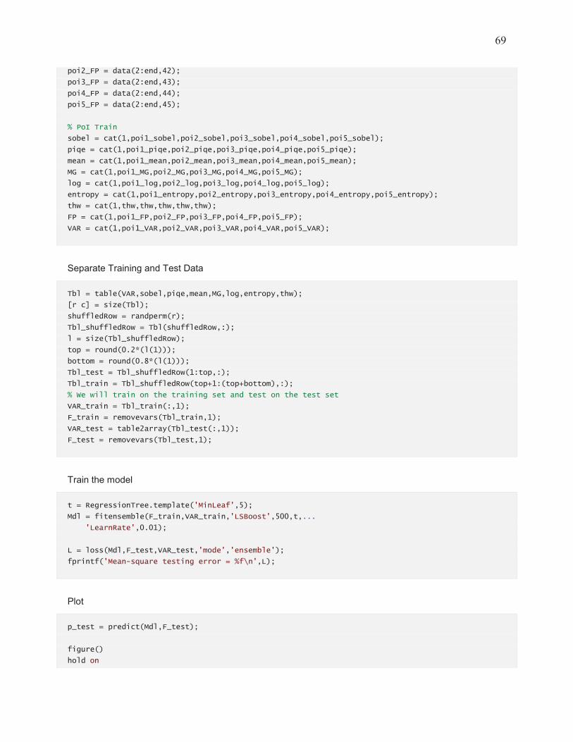
69

poi2_FP = data(2:end,42);

poi3_FP = data(2:end,43);

poi4_FP = data(2:end,44);

poi5_FP = data(2:end,45);

% PoI Train

sobel = cat(1,poi1_sobel,poi2_sobel,poi3_sobel,poi4_sobel,poi5_sobel);

piqe = cat(1,poi1_piqe,poi2_piqe,poi3_piqe,poi4_piqe,poi5_piqe);

mean = cat(1,poi1_mean,poi2_mean,poi3_mean,poi4_mean,poi5_mean);

MG = cat(1,poi1_MG,poi2_MG,poi3_MG,poi4_MG,poi5_MG);

log = cat(1,poi1_log,poi2_log,poi3_log,poi4_log,poi5_log);

entropy = cat(1,poi1_entropy,poi2_entropy,poi3_entropy,poi4_entropy,poi5_entropy);

thw = cat(1,thw,thw,thw,thw,thw);

FP = cat(1,poi1_FP,poi2_FP,poi3_FP,poi4_FP,poi5_FP);

VAR = cat(1,poi1_VAR,poi2_VAR,poi3_VAR,poi4_VAR,poi5_VAR);

Separate Training and Test Data

Tbl = table(VAR,sobel,piqe,mean,MG,log,entropy,thw);

[r c] = size(Tbl);

shuffledRow = randperm(r);

Tbl_shuffledRow = Tbl(shuffledRow,:);

l = size(Tbl_shuffledRow);

top = round(0.2*(l(1)));

bottom = round(0.8*(l(1)));

Tbl_test = Tbl_shuffledRow(1:top,:);

Tbl_train = Tbl_shuffledRow(top+1:(top+bottom),:);

% We will train on the training set and test on the test set

VAR_train = Tbl_train(:,1);

F_train = removevars(Tbl_train,1);

VAR_test = table2array(Tbl_test(:,1));

F_test = removevars(Tbl_test,1);

Train the model

t = RegressionTree.template('MinLeaf',5);

Mdl = fitensemble(F_train,VAR_train,'LSBoost',500,t,...

'LearnRate',0.01);

L = loss(Mdl,F_test,VAR_test,'mode','ensemble');

fprintf('Mean-square testing error = %f\n',L);

Plot

p_test = predict(Mdl,F_test);

figure()

hold on

70

plot(VAR_test,p_test,'+')

xlabel('Measured Log Amplitude Variance','Interpreter','latex')

ylabel('Predicted Log Amplitude Variance','Interpreter','latex')

title('Case 1','Interpreter','latex')

plot(0:1.2,0:1.2,'r-')

axis([0 1.2 0 1.2])

Published with MATLAB® R2019a

Appendix H: Boosted Regression Tree Model Cases 2-6

Boosted - Trained on Fried Parameter

clear;close all;clc

data = xlsread('DATA_UTD_10APR22.xlsx','DATA');

poi1_sobel = data(2:end,6);

poi2_sobel = data(2:end,7);

poi3_sobel = data(2:end,8);

poi4_sobel = data(2:end,9);

poi5_sobel = data(2:end,10);

poi1_piqe = data(2:end,11);

poi2_piqe = data(2:end,12);

poi3_piqe = data(2:end,13);

poi4_piqe = data(2:end,14);

poi5_piqe = data(2:end,15);

poi1_mean = data(2:end,16);

poi2_mean = data(2:end,17);

poi3_mean = data(2:end,18);

poi4_mean = data(2:end,19);

poi5_mean = data(2:end,20);

poi1_MG = data(2:end,21);

poi2_MG = data(2:end,22);

poi3_MG = data(2:end,23);

poi4_MG = data(2:end,24);

poi5_MG = data(2:end,25);

poi1_log = data(2:end,26);

poi2_log = data(2:end,27);

poi3_log = data(2:end,28);

poi4_log = data(2:end,29);

poi5_log = data(2:end,30);

poi1_entropy = data(2:end,31);

poi2_entropy = data(2:end,32);

poi3_entropy = data(2:end,33);

poi4_entropy = data(2:end,34);

poi5_entropy = data(2:end,35);

71

thw = data(2:end,3);

poi5_thw = thw;

poi1_VAR = data(2:end,36);

poi2_VAR = data(2:end,37);

poi3_VAR = data(2:end,38);

poi4_VAR = data(2:end,39);

poi5_VAR = data(2:end,40);

poi1_FP = data(2:end,41);

poi2_FP = data(2:end,42);

poi3_FP = data(2:end,43);

poi4_FP = data(2:end,44);

poi5_FP = data(2:end,45);

PoI Train

sobel = cat(1,poi1_sobel,poi2_sobel,poi3_sobel,poi4_sobel);

piqe = cat(1,poi1_piqe,poi2_piqe,poi3_piqe,poi4_piqe);

mean = cat(1,poi1_mean,poi2_mean,poi3_mean,poi4_mean);

MG = cat(1,poi1_MG,poi2_MG,poi3_MG,poi4_MG);

log = cat(1,poi1_log,poi2_log,poi3_log,poi4_log);

entropy = cat(1,poi1_entropy,poi2_entropy,poi3_entropy,poi4_entropy);

thw = cat(1,thw,thw,thw,thw);

VAR = cat(1,poi1_VAR,poi2_VAR,poi3_VAR,poi4_VAR);

FP = cat(1,poi1_FP,poi2_FP,poi3_FP,poi4_FP);

Separate Training and Test Data

Tbl = table(VAR,sobel,piqe,mean,MG,log,entropy,thw);

[r c] = size(Tbl);

shuffledRow = randperm(r);

Tbl_train = Tbl(shuffledRow,:);

VAR_train = table2array(Tbl_train(:,1));

F_train = removevars(Tbl_train,1);

sobel = poi5_sobel;

piqe = poi5_piqe;

mean = poi5_mean;

MG = poi5_MG;

log = poi5_log;

entropy = poi5_entropy;

FP = poi5_FP;

VAR = poi5_VAR;

thw = poi5_thw;

Tbl = table(VAR,sobel,piqe,mean,MG,log,entropy,thw);

[a c] = size(Tbl);

shuffledRow2 = randperm(a);

Tbl_test = Tbl(shuffledRow2,:);

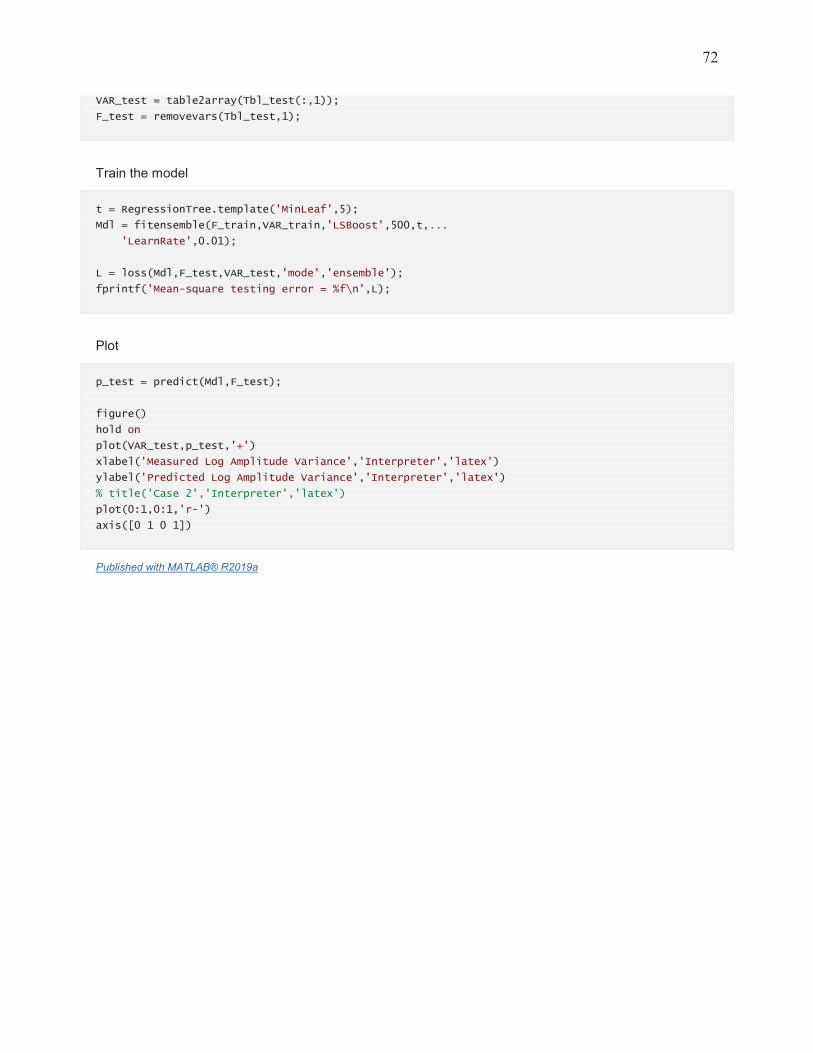
72

VAR_test = table2array(Tbl_test(:,1));

F_test = removevars(Tbl_test,1);

Train the model

t = RegressionTree.template('MinLeaf',5);

Mdl = fitensemble(F_train,VAR_train,'LSBoost',500,t,...

'LearnRate',0.01);

L = loss(Mdl,F_test,VAR_test,'mode','ensemble');

fprintf('Mean-square testing error = %f\n',L);

Plot

p_test = predict(Mdl,F_test);

figure()

hold on

plot(VAR_test,p_test,'+')

xlabel('Measured Log Amplitude Variance','Interpreter','latex')

ylabel('Predicted Log Amplitude Variance','Interpreter','latex')

% title('Case 2','Interpreter','latex')

plot(0:1,0:1,'r-')

axis([0 1 0 1])

Published with MATLAB® R2019a