1

A Temporal Modelling Environment for Internally Grounded

Beliefs, Desires and Intentions*

Catholijn M. Jonker Vrije Universiteit Amsterdam1

Jan Treur Vrije Universiteit Amsterdam1, Utrecht University2

Wouter C.A. Wijngaards Vrije Universiteit Amsterdam 1

In this paper the internal dynamics of mental states, in particular states based on beliefs, desires and intentions, is formalised using a temporal language. A software environment is presented that can be used to specify, simulate and analyse temporal dependencies between mental states in relation to traces of them. If also relevant data on internal physical states over time are available, these can be analysed with re-spect to their relation to mental states as well.

1. Introduction Dynamics has become an important focus within Cognitive Science in recent years; e.g., (Port & van Gelder, 1995). As one of the aspects, the dynamics of the interaction with the external world, and its implications for the represen-tational content and dynamics of mental states have received attention; e.g., (Bickhard, 1993; Christensen & Hooker, 2000). Another important aspect is the internal dynamics of mental states, as can be found, for example in the dynamics of intentional notions (such as beliefs, desires and intentions) and their interaction with each other and with the external world. An example of a pattern for such internal dynamics is: if a desire and an additional reason (in the form of a belief about the world) to do some action are both present, then the intention to do the action is generated.

In this paper the internal dynamics of mental states based on beliefs, de-sires and intentions (which also may include dynamics of the interaction of mental states with the external world) is addressed. A modelling environ-

* In Cognitive Systems Research Journal, vol. 4(3), 2003, pp. 191-210.

2

ment is presented that can be used to specify, simulate and analyse models for these dynamics, taking into account mental aspects (mind), physical as-pects (matter), or both. A basic notion underlying the modelling is the notion of functional role or profile of a mental state. In (Bickle, 1998), the functional profile of a mental state is considered as (p. 198) ‘… the set of all causal paths running through it.’, and mental states are assigned (pp. 205-206) ‘… a place in an abstract, systematically connected network running from sensory to behavior peripheries, in terms of the states and events that cause their occur-rence and the subsequent states or events they cause.’

A question is how such functional roles can be modelled in a precise and formal manner that stays close to the original idea. In this paper functional roles of belief, desire and intention states are modelled in a temporal language in such a manner that causal relationships are formalised by temporal de-pendencies they entail. Since dynamics is a phenomenon occurring over real time, the real numbers are used as time frame; no approximation by a se-quence of fixed discrete time steps is needed. The temporal language can be used on the one hand for the specification of temporal relationships between mental states involving beliefs, desires and intentions (and between mental states and the external world). Such a temporal specification can be used to express a theory for these dynamics. On the other hand the language is the basis of a software environment that has been implemented and which can be used for the simulation and analysis of the internal dynamics.

Simulation takes place within this software environment by generating consequences over time from the specified set of temporal relationships, according to the paradigm of executable temporal logic (Barringer et al., 1996). To predict the internal dynamics, the software takes the temporal relationships, some initial values, and a pattern of environment dynamics to produce implied traces of internal belief, desire and intention states. Analysis of given traces (in comparison to certain temporal relationships) is sup-ported by the software environment as well. For example, these given traces can have the form of successively attributed intentional states over time. The automated support displays any discrepancies between such data and a background theory of the dynamics expressed by (assumed) temporal rela-tionships. Another use of the software environment is the analysis of the relationship between mental and physical internal states. If observations (e.g., by advanced scanning techniques) can be made of the physical states assumed to be related to mental states, these empirical physical traces can be used as input, after which the software environment generates the related mental traces and checks the temporal relationships.

In Section 2 the intentional notions on which the paper focuses are intro-duced; for each type of intentional notion its functional role with respect to the other notions is discussed informally. In Section 3 the formalisation for the dynamics is presented. An example is discussed in Section 4. Subse-quently in Section 5 the software environment, and some results are pre-

3

sented. Section 6 addresses the use of the environment when relevant physi-cal internal state data over time are available. Section 7 shows the use of the software environment to analyse cognitive development results for children, while Section 8 concludes with a discussion.

2. The Intentional Notions Addressed The intentional notions from the BDI model (belief, desire and intention), are addressed in a static manner in e.g. (Rao & Georgeff, 1991; Linder, Hoek & Meyer, 1996); in our approach they are used in temporal perspective, see Figure 1.

Beliefs are based on observation of the outside world in the present or in the past. Beliefs are modified in response to changes perceived in the external world. Beliefs can be incorrect (a false belief), e.g. due to some faulty sensory input. A belief means that the agent thinks that some property holds. Also a belief can mean that the agent thinks that some property does not hold. Ex-amples are that the agent has the belief that cheese is present, or that the agent has the belief that no screen is present.

In principle it is possible to have both the belief that something holds and the belief that it does not hold, at the same time. Since such a state of affairs may have deplorable consequences for the agent, this possibility is excluded; see Section 3 for this and other details of the semantics.

Desires are states of the world or changes to the world that are de-sired. Desires are formed based on the agent’s history. Desires are created and stay in existence for a while. The desires the agent has at one time can conflict with each other. An example of desires is the desire to eat food.

β(x, pos) : denotes that the agent has the belief that x holds. β(x, neg) : denotes that the agent has the belief that x does not hold. β(cheese_present, pos) : denotes that the agent has the belief that cheese_present holds; that cheese is present. β(screen_present, neg) : denotes that the agent has the belief that screen_present does not hold; that the screen is not present.

δ(x) : denotes that the agent has a desire for x. The desire can be for a situation or an action. δ(eat_food) : denotes that the agent has a desire to eat food.

4

Agent desires C

resulting fromhistory ofthe agent

Agent has reasons to pursue B

change of beliefs(by observation or deduction)

Agent intends B, which realizes CAgent believes it has the opportunity to do AAgent performs A, which realizes B

desire and reason leading to intention

intention and belief in opportunity

leading to action

because oflack of reason

because oflack of intention

and/or opportunity

timeabsent present

Figure 1. BDI notions over time.

From the set of desires that exist in a given situation some can be chosen

to be pursued by creating an intention for them. For example, when a desire exists and an additional reason ρ (i.e., a particular co-occurrence of beliefs) also holds then an intention to fulfil the desire is created. This intention lasts until the desire or the additional reason for it disappears. For example, the presence of cheese can serve as an additional reason for the agent to intend to eat. Additional reasons perform at least two functions. Firstly, they inhibit the selection of conflicting intentions. Secondly, they cause the selection of particular intentions when those intentions are appropriate. The first and second uses can over-lap. For example, if an animal obtains food, it could intend to eat it, or store it for later use. The intention to store the food for later, could need the reason that winter is approaching, selecting the intention when appropriate. The intention to store the food is used under the condition (additional reason) that it is not hungry, preventing a conflict with the intention to eat the food, which it only does when hungry.

The intentions are states or changes in the world that are in-tended to be accomplished. The intentions of an agent at a particu-lar time do not conflict with each other. When the intention exists and it is believed that an opportu-nity ο presents itself, the action is performed. For example, after hav-ing the intention to eat food, the actual action occurs if the agent believes that there is no screen in the way. The action is undertaken until the intention or the belief in the op-portunity for it disappears. Actions can have the intended effect, but can also fail or produce unexpected results.

ι(x) : denotes that the agent has the intention for x. θ = α(x) : denotes an action atom of the form α(x). It refers to process x

in the external world. β(ο1) = β(screen_present, neg) : denotes a belief in an opportunity, the op-portunity is the absence of a screen; ο1 = ¬screen_present.

ρ1 = β(cheese_present, pos) : denotes an additional reason, composed of the belief that cheese is present.

5

3. Dynamical Formalisation In BDI-logics such as (Rao & Georgeff, 1991; Linder et al., 1996) internal processes are considered instantaneous. However, a more sincere formalisa-tion is obtained if also internal processes take time. In this paper real time is used (represented by real numbers); time is not measured in computational steps. Real time temporal relationships are defined that take into account the delay between cause and effect, together with the durations of those cause and effect situations. The delay and durations may be measured. In this set-ting, the BDI-notions can be defined by the functional role they play. In the following the term agent is used to refer to the subject and system is used to refer to both the agent and the external world together. Intervals of real numbers are denoted like: [x, y) meaning {p ∈ |R | p ≥ x ∧ p < y}. Thus, ‘[’ or ‘]’ stands for a closed end of the interval, and ‘(’ or ‘)’ stands for an open end of the interval.

Definition (state properties) The states of the system are characterised by state properties. The state prop-erties are formalised using (logical) formulae over a specific ontology. For an ontology Ont, the set of atoms AT(Ont) contains the atomic properties expressed in terms of the ontology. The set of state properties SPROP(Ont) contains all the propositional formulas built out of the atoms using standard propositional connectives. More specifically, the following ontologies are used. Firstly, world state properties express properties of a particular situation in the mate-rial world, using ontology EWOnt. Secondly, the internal physical state prop-erties of the agent are expressed using IntOntP. The combined physical ontol-ogy is OntP = def EWOnt ∪ IntOntP. Thirdly, the ontology for internal mental state properties is denoted by IntOntM. The ontology for all state properties is de-noted by AllOnt =def EWOnt ∪ IntOntP ∪ IntOntM.

Definition (states) a) A physical state P of the system is an assignment of truth values {true,

false} to the set of physical state atoms AT(OntP) of the system. The set of all possible physical states is denoted PS.

b) A (partial) mental state M of the system is an assignment of truth values {true, false, unknown} to the set of internal mental state atoms, AT(IntOntM). The set of all possible mental states is denoted by MS.

c) At each time-point the system is in one state. This state is from the set States =def PS x MS. d) The standard satisfaction relation |== between states and state properties is used: S |== ϕ means that property ϕ holds in state S.

6

Note that in contrast to mental states, for physical states the truth value unknown is excluded: no indeterminate world states are considered. Allow-ing indeterminate physical states simply can be obtained by allowing truth value unknown as well for physical states.

Three-valued states are useful in simulation. Suppose states are two-valued, then if a new state is computed from the previous one, and the speci-fication does not provide a truth value true or false for a given state prop-erty, then this process is stuck unless a choice is forced. For example, this can be forced by a form of the closed world assumption (e.g., in Concurrent MetateM: Fisher, 1994): making all unknown properties false. Another op-tion would be to require that the specification is complete in the sense that it provides truth values true or false in the next state for all possible situations. This may make the specification complex as for all atomic state properties assignments have to be made explicit. Allowing the truth value unknown avoids these problems.

Definition (traces) The system when viewed over a period of time, will produce several states consecutively. The function T returning the state for each time point is called a trace, T: |R → States. The set of all possibly occurring traces, i.e. respecting the world’s laws, is denoted W.

The behaviour of the agent and environment is defined by a set of traces. Temporal relationships be-tween the state properties over time specify such a set of traces: they express certain constraints on the relative timing of the occurrence of state proper-ties. These constraints on the timing reflect a causal relationship between the arguments.

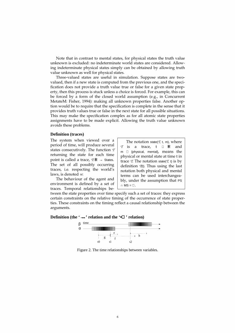
Definition (the ‘ →→→→→→→→’ relation and the ‘ ••••’ relation)

αβ

t1

e

g h

t2

time

ft0

Figure 2. The time relationships between variables.

The notation state(T, t, m), whereT is a trace, t ∈ |R and m ∈ {physical, mental}, means the physical or mental state at time t in trace T. The notation state(T, t) is by definition T(t). Thus using the last notation both physical and mental terms can be used interchangea-bly, under the assumption that PS

∩ MS = ∅.

7

Let α , β ∈ SPROP(AllOnt). The state

property α follows state property β, denoted by α →→e, f, g, h β, with time delay interval [e, f] and duration parameters g and h denotes that:

if property α holds for a while (g), then some time (between e and f) later property β will hold for a while (h).

Conversely, the state property β

originates from state property α, denoted by α •e, f, g, h β, with time delay in [e, f] and duration parame-ters g and h denotes that:

if property β holds for a while (h), then some time (between e and f) earlier property α will hold for a while (g).

If both α →→e,f,g,h β, and α •e,f,g,h β hold, this is denoted by: α •→→e,f,g,h β

pronounced α leads to β.

The relationships between the variables α, β, e, f, g, h, t0, t1 and t2 are de-picted in Figure 2. Further details of this formalisation can be found in Ap-pendix A.

Definition (uninterrupted) Loosely phrased, uninterrupted means that given ϕ •→→ ψ, when ϕ holds for an uninterrupted length of time, then ψ will also hold for an uninterrupted length of time, with-out gaps.

Let ϕ, ψ ∈ SPROP(AllOnt). The relation-ship ϕ •→→e,f,g,h ψ is uninterrupted if:

∀T ∈ W ∀t0 ∀t1>t0: if (∀t ∈ [t0, t1) : state(T, t) |== ϕ) then

(∀t2,t3 ∈ [t0+g+e, t1+f+h]:

state(T, t2) |== ψ ∧ state(T, t3) |== ψ ) � (∀t4 ∈ (t2, t3): state(T, t4) |== ψ).

Note that if ϕ •→→e,f,g,h ψ and e + h ≥ f, then ϕ •→→e,f,g,h ψ is uninterrupted. Based on the general notions introduced, next the notions internal belief

representation, internal intention representation and internal desire repre-sentation are defined.

Definition (internal belief representation) Let ϕ ∈ SPROP(OntP) be a physical state property.

a) The internal mental state property β ∈ SPROP(IntOntM) is called an inter-nal belief representation for ϕ with time delay e and duration parameters f, g if: ϕ •→→e,f,g,h β .

∀T ∈ W ∀t1:

[∀t ∈ [t1 - g, t1) : state(T, t) |== α �

∃d ∈ [e, f] ∀t ∈ [t1 + d, t1 + d + h) :

state(T, t) |== β ]

∀ T ∈ W ∀ t2:

[∀t ∈ [t2, t2 + h) : state(T, t) |== β �

∃d ∈ [e, f] ∀t ∈ [t2 - d - g, t2 - d) :

state(T, t) |== α]

8

b) Two belief representations β1 and β2 are exclusive if they never hold at the same time.

Formally this is denoted as: ∀T ∈ W: ¬∃t: state(T, t) |== β1 ∧ β2.

In a) of this definition the →→ part is necessary, as the occurrence of exter-nal state ϕ should lead to the creation of the belief β. The • part must also hold, since a belief β must have an explanation of having being created, in this case ϕ. This consideration also holds for intentions and desires in an analogical fashion.

When the world situation suddenly changes, the beliefs may follow suit. The belief β1 and the belief β2 of two opposite world properties should not hold at the same time; they should be exclusive. As the external world state fluctuates, the beliefs should change accordingly, but never should there be both a belief for a world property and a belief for the opposite world prop-erty at the same time. If two belief representations for opposite world prop-erties are exclusive, this inconsistency is avoided, and the belief representa-tions are called non-conflicting.

Definition (internal intention representation) Let α ∈ SPROP(OntP) be a physical state property, β ∈ SPROP(IntOntM) a belief representation for α and θ ∈ SPROP(IntOntM) an action atom. The internal men-tal state property γ ∈ SPROP(IntOntM) is called an internal intention representa-tion for action atom θ and opportunity α with delay e, f and duration parame-ters g, h if γ ∧ β •→→e,f,g,h θ.

Definition (internal desire representation) Let ρ ∈ SPROP(OntP) be a physical state property, β a belief representation for ρ and γ an intention representation. The internal mental state property δ ∈

SPROP(IntOntM) is an internal desire representation for intention γ and additional reason ρ with delay e, f and duration parameters g, h if δ ∧ β •→→e,f,g,h γ.

4. An Example Formalisation In order to demonstrate the formalisation and automated support presented in this paper, a simple example description is put forward. In this example, the test subject is a common laboratory mouse, that is presented with cheese. Mostly, the mouse will try to eat the cheese, but a transparent screen can block access to the cheese. First, an intentional perspective on the mouse is constructed. Then, assuming a mouse-brain-scanning-technique, it is ana-lysed how specific brain area activity can be correlated to the intentional notions.

The formalised physical external world description of this experiment has two properties; screen_present and cheese_present. The internal physical state has the property hungry.

9

The intentional description of the mouse makes use of the following be-liefs on the relevant parts of the world for this experiment: β(hungry, pos), β(hungry, neg), β(screen_present, pos), β(screen_present, neg), β(cheese_present, pos) and β(cheese_present, neg). These beliefs are all based on perceptions by the mouse.

The beliefs should persist uninterruptedly if the perceptions stay the same. So if ϕ holds in the interval [t0, t2) then the belief will hold in a uninter-rupted resultant interval. The timing parameters of the belief observations indeed guarantee that a uninterrupted belief representation is obtained.

When the world situation changes, the beliefs change. The g and h of the belief generation relations are chosen equal, so that the belief representations are non-conflicting: the belief in a world property starts to be there exactly at the same time the belief in the opposite property stops to be there.

Furthermore, the intentional description includes desires. If the mouse is hungry, it desires to eat, δ(eat_food). When sufficient additional reason, ρ1, is present – the belief that there is cheese – the mouse will intend to eat the cheese, ι(eat_cheese). When the mouse believes that the opportunity, ο1, pre-sents itself, the screen not being present, the mouse will eat the cheese, the action denoted by α(eat_cheese).

The temporal relationships for the intentional description of the mouse are given below. All e, f, g and h values for the temporal relationships are given in sequence, after the •→→ symbol, in a certain time unit (e.g., 0.1 sec-ond).

.......................................... Sensing............................................ hungry •→→1, 5, 10, 10 β(hungry, pos) ∧ ¬β(hungry, neg).

¬hungry •→→1, 5, 10, 10 β(hungry, neg) ∧ ¬β(hungry, pos).

cheese_present •→→1, 5, 10, 10 β(cheese_present, pos)

∧ ¬β(cheese_present, neg).

¬cheese_present •→→1, 5, 10, 10 β(cheese_present, neg)

∧ ¬β(cheese_present, pos).

screen_present •→→1, 5, 10, 10 β(screen_present, pos)

∧ ¬β(screen_present, neg).

¬screen_present •→→1, 5, 10, 10 β(screen_present, neg)

∧ ¬β(screen_present, pos).

..................................Internal Processes................................... β(hungry, pos) •→→1, 5, 10, 10 δ(eat_food).

δ(eat_food) ∧ ρ1 •→→1, 5, 10, 10 ι(eat_cheese).

ι(eat_cheese) ∧ ο1 •→→1, 5, 10, 10 α(eat_cheese).

ρ1 = β(cheese_present, pos). ο1 = β(screen_present, neg).

...................................Wor ld Processes..................................... α(eat_cheese) ∧ cheese_present •→→1, 5, 10, 10 ¬hungry.

10

In order to derive the converse of the previous temporal relationships, a

temporal variant of Clark’s completion is used (Clark, 1978).

¬β(hungry, pos) •→→1, 5, 10, 10 ¬δ(eat_food).

¬(δ(eat_food) ∧ ρ1) •→→1, 5, 10, 10 ¬ι(eat_cheese).

¬(ι(eat_cheese) ∧ ο1) •→→1, 5, 10, 10 ¬α(eat_cheese).

¬(α(eat_cheese) ∧ cheese_present) •→→1, 5, 10, 10 hungry. At the start of derivation the intentional notions will be false, in particular

the mouse initially does not believe anything. The starting value of each property is given for e + λ(f-e) + g time units.

5. Implementation of the Software Environment A software environment has been made which implements the temporal formalisation of the internal dynamic behaviour of the agent. First the ap-proach is introduced, then the program will be briefly reviewed, after which some of the results are discussed.

5.1. Approach The simulation determines the consequences of the temporal relationships forwards in time. In order to make simulation efficient, long intervals of results are derived when starting from long intervals. By applying addi-tional conditions (i.e., e+h ≥ f), the derivation of longer intervals becomes possible, see Section 3 (uninterrupted). The logical relationships thus are taken to be uninterrupted, avoiding unnecessary work for the derivation software.

The delay value λ can either be chosen randomly within the interval [e, f] each time a relationship is used, or the λ can be fixed to a value (0.25 in the example). Selecting either a random or fixed λ enables thorough investiga-tion of the consequences of a particular model.

5.2. The Temporal Simulation Program Following the paradigm of executable temporal logic, cf. (Barringer et al., 1996), a 2700 line simulation program was written in C++ to automatically generate the consequences of the temporal relationships. The program is a special purpose tool to derive the results reasoning forwards in time, as in executable temporal logic. After a short look at the method of forward deri-vation, the specification of the derivation rules is presented.

In order to derive the consequences of the temporal relationships within a specific interval of time, a cycle is performed, starting at time 0. For the set of rules the earliest starting time of the antecedent for each rule, for which the consequent does not already hold, is computed. The rule with the earli-

11

est start time of the antecedent is chosen. If several rules have an antecedent at exactly the same time, the rule appearing the first in the specification is taken. This rule is then fired at that time, adding the consequent to the trace. The cycle is restarted, only looking for antecedents at or after the fire time point, as effects are assumed to occur simultaneously or after their causes. This continues until no more rule can be fired, or the fire time is at or after the end time of the simulation interval.

The program reads a specification of the temporal rules from a plain text file. The maximum time for derivation is also given, the interval [0, MaxTime). In order to specify facts about the world, (periodic) intervals can be given. The functions not(), and(,), and or(,) can be used to make more complex proper-ties from atoms. The properties have and, or and not given in prefix ordering for the program (instead of infix). In prefix ordering, a function is given be-fore its arguments, i.e. and(a, b) instead of (a and b). In the program belief is used to denote β, desire for δ, intention for ι and performs for α. The •→→ relation is specified using LeadsTo, followed by the e, f, g and h values. The relationships specified are implied by the relationships presented in Section 4. Note that the • part of the relation, originating from, is not used by the program, as only forward deduction is performed. An example of a rule, see the relationship in Section 4 that derives ι(eat_cheese) from δ(eat_food), is:

Rule LeadsTo delay 1 5 10 10 and( desire(eat_food) , belief(cheese_present,pos) ) o->> intention(eat_cheese)

5.3. Results The graph in Figure 3 shows the reaction of the mouse to changes in the environment. Time is on the horizontal axis. The world state properties and the intentional notions are listed on the vertical axis. The parameter λ is fixed at 0.25. A dark box on top of the line indicates the notion is true, and a lighter box below the line indicates that the notion is false.

Figure 3. Results from the implementation when the environment is set initially to

have cheese and a screen. Later the screen is removed.

12

As can be seen, the mouse is not hungry at the very start, but quickly be-

comes hungry. It desires to eat the cheese, and intends to do so, but the screen blocks the opportunity to do so. When the screen is removed, the mouse eats. After a while it stops eating, as it is not hungry anymore. Subse-quently it enters a cycle where it becomes hungry, eats, and becomes hungry again.

5.4. Intentional Attribution Checker Another program, of about 4000 lines in C++, has been constructed that takes an existing trace of behaviour as input and creates an interpretation of what happens in this trace and a check whether all temporal relationships hold. The program is configured (amongst others) by giving a set of inten-tional temporal relationships, see Section 4 for example relationships. The program marks any deficiencies in the trace compared with what should be there due to the temporal relationships.

Appendix C contains an automatically generated example interpretation of a trace. All temporal relationships hold in this trace. If a relationship does not hold completely, this is marked by the program. The program produces yellow marks for unexpected events. At these moments, the event is not produced by any temporal relationship; the event cannot be explained. The red marks indicate that an event has not happened, that should have hap-pened.

In addition to checking whether the rules hold, the checker produces an informal reading of the trace. The reading is automatically generated, using a simple substitution, from the information in the intentional trace.

6. Mind and Matter: Internal Physical versus Mental States In the formalisation, each internal state has a mental state and a physical state portion. The physical state is described by a set of (real number) value assignments to continuous variables. The automated support also supports the assignment of internal physical properties to intentional notions; also material data can be used as input. For the assignment of physical properties to intentions, each intentional property has one physical property associated. The values true and false of the intentional notion are assigned to particular ranges of values of the material in the data.

For the example, it is assumed that a scanner provides signal intensities for different brain areas. Some of these may correlate with the intentions as described above. An assumed example assignment of intentional notions to the signal intensities of specific brain areas is given in Table 1.

13

Table 1. Related physical and mental state properties.

Intentional notion in SPROP(IntOntM)

Physical condition in SPROP(IntOntP)

β(hungry, pos) intensity of area_01 ≥ 1.0 β(hungry, neg) intensity of area_02 < 1.0 β(cheese_present, pos) intensity of area_03 ≥ 1.0 β(cheese_present, neg) intensity of area_04 < 1.0 β(screen_present, pos) intensity of area_05 ≥ 1.0 β(screen_present, neg) intensity of area_06 < 1.0 δ(eat_food) intensity of area_07 ≥ 1.0 ι(eat_cheese) intensity of area_08 ≥ 1.0 α(eat_cheese) intensity of area_09 ≥ 1.0

The simulation program, having derived an intentional trace, can output

a physical trace based on it. The physical trace consists of the possible ranges of values for all physical state variables in each time-interval.

The checker can read back a physical trace as generated by the simulator, but it can also read back a trace where for time-points a value for each physical state variable is given. It will then interpret this physical trace, comparing the given (range of) value(s) to the true and false ranges as given per intentional notion. It will then check whether all the given temporal rela-tionships hold correctly.

Using the interpretation and checking of relationships the program can assist in the verification of hypothetical assignments of physical properties to intentional notions, and the verification of hypothetical intentional tempo-ral relationships.

7. Relations to Empirical Work In this section we will look at how our approach can be related to experi-mental findings about cognition of small children. In the literature reports of many empirical studies of intentional attribution can be found; e.g., (Zadny & Gerard, 1974; Malle & Knobe, 1997; Carpenter, Akhtar & Tomasello, 1998; Gergely, Nádasdy, Csibra & Bíró, 1995; Feinfield, Lee, Flavell, Green & Flav-ell, 1999), for an overview, see (Baldwin & Baird, 2001), or (Malle, Moses, and Baldwin, 2001). First an experiment with children at 12 months of age is discussed, and next an experiment with 3 to 4 year olds is addressed. The aim is to see if the experimental settings can be described using temporal relationships, and if the analysis by the software is coherent with the out-comes of the experiments.

7.1. The Intentional Stance at 12 Months of Age In the experiment discussed, see (Gergely, Nádasdy, Csibra & Bíró, 1995),

young children were shown a variety of action sequences. The children ha-bituated to the sequences. The dishabituation was measured when the action

14

sequence was altered in order to measure the child’s interest, the newness, in relation to whether the action sequence shows rational or nonrational action. Based on the outcomes, Gergeley et al. conclude that children at 12 months of age are able to take an intentional stance (Dennet, 1987) towards agent-like objects.

a) b)

p pa

b

Figure 4. Two examples of rational behaviour. In a) the small circle moves in a

straight line to p. In b) the small circle jumps.

a)

b) Figure 5. Traces of the rational habituation examples, obtained from a simulation

of the temporal relationships from the first model. In a) the obstacle is present, while in b) the obstacle is absent. Delay parameter λ is fixed at 0.5 in both simulations.

More specifically, the experiments were performed as follows. In the ex-

periment two black circles are shown, pulsating in sequence to impress the children with the agent-likeness of the circles. The expanding and contract-ing of the diameter in turn-taking sequence is meant to resemble communi-cation. Then, the small circle would move to the larger circle, where they would pulsate again. Adults typically describe this as a mother calling her child, who then comes to her. An obstacle can impede the movement to-

15

wards the bigger circle. The smaller circle could jump over the obstacle or use a direct line towards the bigger circle, see Figure 4. Showing a large number of different variants of rational behaviour (i.e., jump if obstacle is present, a straight line in the other case), the children became habituated to such behavioural patterns.

This experimental setup was modelled according to our approach by us-ing temporal relations. According to the intentional stance the behaviour of the smaller circle can be modelled in two ways. First, the smaller circle has the desire to be close to the bigger circle, and it can intend to go to the bigger circle (position p), deciding on the specific action (jump or straight line) based on the opportunity. Second, the smaller circle has the desire to be close to the bigger circle, and it can intend (based on an additional reason) to either go to p using a jump or via a straight line. Both ways will be discussed in turn.

In both models position p is the position of the bigger circle. Route a to p is the direct route, route b to p is where the smaller circle jumps. Route a fails when the obstacle is present. In the world, the obstacle is said to be present when a block is between the smaller and larger circle. The smaller circle is taken to desire to be at p. The temporal relationships for the first model are:

..................................... Sensing .................................... 1 obstacle •→→1,5,10,10 β(obstacle,pos) ∧ ¬β(obstacle,neg).

2 ¬obstacle •→→1,5,10,10 β(obstacle,neg) ∧ ¬β(obstacle,pos).

......................................Desires..................................... 3 δ(be_at_p).

....................Rules to determine intentions................... 4 δ(be_at_p) ∧ ρ •→→1,5,10,10 ι(go_to_p). ρ =def true.

...................... Rules to determine actions..................... 5 ι(go_to_p) ∧ ο1 •→→1,5,10,10 α(go_by_a).

6 ι(go_to_p) ∧ ο2 •→→1,5,10,10 α(go_by_b). ο1 =def β(obstacle,neg). ο2 =def β(obstacle,pos).

.................................Action effects................................ 7 α(go_by_a) ∧ ¬obstacle •→→1,5,10,10 at_p.

8 α(go_by_b) •→→1,5,10,10 at_p.

The habituation phase for the experiments for rational movement can be derived in an automated manner using simulation from the temporal rela-tions. In Figure 5 some training simulations when the obstacle is present and absent are depicted.

16

Figure 6. The experimental nonrational trace analysed by the checking software.

In this trace route b is used, even though the obstacle is absent. In addition the checking software can be used to analyse the testing ex-

perimental sequence of actions. The testing sequence of actions, where the smaller circle moves towards the bigger circle using path b, jumping, despite the fact that there is no obstacle, has been fed to the checker implementation. The testing behaviour is the behaviour depicted as in Figure 4b, but without the obstacle present. The resulting analysis output is in Figure 6 and Table 3.

In Figure 6 it can be seen that the action to move using route a is ex-pected, but was not found in the trace (red colour). Instead, the action to move using route b was found, unexpectedly (yellow colour).

Table 3 contains the formal intentional interpretation, rule detection and generated informal explanation of the trace.

17

Table 3. The automatically generated explanation of the trace

from Figure 6.

time formal intentional interpretation

rule detection (in retrospect) generated informal explanation

0.00 obstacle: f δ(be_at_p): t

Start of antecedent interval for rule 2. Start of consequent interval for rule 3. Start of antecedent interval for rule 4.

No obstacle is present. It desires to be at p.

15.00 ι(go_to_p): t β(obstacle,pos): f β(obstacle,neg): t

Start of consequent interval for rule 4. Start of consequent interval for rule 2.

It intends to go to p. It does not believe that the obstacle is present. It believes that it is not the case that the obstacle is present.

30.00 α(go_by_b): t

Start of unexpected interval, no rule can explain α(go_by_b). Start of antecedent interval for rule 8. Expected α(go_by_a), part of the consequent of rule 5, which should have started at this time.

It proceeds to go to p by b. Atom α(go_by_b) started to violate the given rules here. Atom α(go_by_a) started to violate the given rules at this time.

45.00 at_p: t Start of consequent interval for rule 8. It is at p. 100.00 β(obstacle,neg): u

δ(be_at_p): u ι(go_to_p): u α(go_by_b): u at_p: u β(obstacle,pos): u obstacle: u

End of consequent interval for rule 2. End of consequent interval for rule 3. End of antecedent interval for rule 4. End of consequent interval for rule 4. End of unexpected interval, no rule can explain α(go_by_b). End of antecedent interval for rule 8. End of consequent interval for rule 8. Expected α(go_by_a), part of the consequent for rule 5, which should have ended at this time. End of antecedent interval for rule 2.

Atom α(go_by_b) stopped to violate the given rules here. Atom α(go_by_a) stopped to violate the given rules here.

The second possible model of this experiment is when there is not a sin-

gle intention to go to p, but two intentions are possible, to go to p by a or by b. This means that the rules to generate intentions and the rules to generate actions change slightly. The temporal relationships for this model are:

18

..................................... Sensing .................................... obstacle •→→1,5,10,10 β(obstacle,pos) ∧ ¬β(obstacle,neg).

¬obstacle •→→1,5,10,10 β(obstacle,neg) ∧ ¬β(obstacle,pos).

......................................Desires..................................... δ(be_at_p).

....................Rules to determine intentions................... δ(be_at_p) ∧ ρ1 •→→1,5,10,10 ι(go_to_p_by_a).

δ(be_at_p) ∧ ρ2 •→→1,5,10,10 ι(go_to_p_by_b). ρ1 =def β(obstacle,neg). ρ2 =def β(obstacle,pos).

...................... Rules to determine actions..................... ι(go_to_p_by_a) ∧ ο1 •→→1,5,10,10 α(go_by_a).

ι(go_to_p_by_b) ∧ ο2 •→→1,5,10,10 α(go_by_b). ο1 =def β(obstacle,neg). ο2 =def true.

.................................Action effects................................ α(go_by_a) ∧ ¬obstacle •→→1,5,10,10 at_p.

α(go_by_b) •→→1,5,10,10 at_p.

This model will also predict the same training examples on the basis of the different world states. The simulation of this is shown in Figure 7. The internal state can be seen to differ from Figure 4.

a)

b) Figure 7. Traces of the rational habituation examples, obtained from a simulation

of the temporal relationships from the second model. In a) the obstacle is present,

19

while in b) the obstacle is absent. Delay parameter λ is fixed at 0.5 in both simula-tions.

The checking software has been used to analyse the experimental nonra-

tional action sequence on the basis of the second model as well. Two traces are analysed, one where the intention to go to p by a holds, and one where the intention to go to p by b holds. The resulting pictures are in Figure 8. In Figure 8a it can be seen that the intention to use route a is expected, since there is no obstacle. But the action to use route b is unexpected (yellow), the action to use route a is expected but absent (red). In Figure 8b the intention to use route b is assumed, but would not rationally be expected (yellow). The shorter route a would be expected, but was not intended (red). The action to perform route b after intending to do so is expected, however, as it is a ra-tional conclusion (from an irrational intention).

Summarizing, a model has been made for the mental state of the smaller circle. The behaviour of the smaller circle in the experiments can be simu-lated and analysed by the software environment. The simulation can dupli-cate the rational behaviour of the smaller circle. Furthermore, just like the children, the analysis pointed out problems in the nonrational behaviour, showing unexpected and expected but absent intervals in the behavioural trace.

a)

b)

Figure 8. The nonrational trace analysis using the relationships in the second model. In a) the intention to go to p by route a is assumed. In b) the intention to use

route b is assumed.

20

7.2. Understanding of Intentionality by Children of 3 to 4 Years Old In a study by (Feinfield, Lee, Flavell, Green & Flavell, 1999) the understand-ing of intentions of 3 to 4 year old children was examined. The children were told a story, accompanied by cute pictures, and asked questions about the child in the story. Several variations of the same type of story were used, and one is formalized below.

In this story, Jason wants to go to the mountains because he likes to play in the snow. He does not want to go play football because he does not like football. But his mom tells him to change into his football uniform and go to the football field. Jason thinks for a minute, and sadly puts on his football uniform. Jason gets on the bus to the football field. But the bus driver gets lost… and stops at the mountains.

After this story, the children were asked where Jason tried to go to, where he thought he was going to go and where he liked to go. Children of 3 years old performed badly at this, but 4 year old children often gave the correct answers.

Also this setting has been modelled using our software environment. The temporal relationships for this model are:

......................................Desires..................................... 0 δ(mountains). 1 ¬δ(football).

....................Rules to determine intentions................... 2 δ(football) •→→1,5,10,10 ι(football).

3 δ(mountains) •→→1,5,10,10 ι(mountains).

...................... Rules to determine actions..................... 4 ι(football) •→→1,50,10,10 α(wear_uniform).

5 ι(football) •→→11,15,10,10 α(goto_field).

6 ι(mountains) •→→1,5,10,10 α(goto_mountains).

.................................Action effects................................ 7 α(wear_uniform) •→→0,5,10,1000 wearing_uniform.

8 α(goto_field) •→→21,25,10,10 at_footballfield.

9 α(goto_mountains) •→→21,25,10,10 at_mountains.

The analysis of the trace corresponding to the storyline is in Figure 10. The desire to go to the mountains can be seen to hold, and the desire to play football not to hold. The intention to go to the mountains is expected, but does not happen (red). Instead, the intention to go play football unexpect-edly happens (yellow). From the intention to play football, the action to wear a football uniform is expected (green), and the action to take the bus to the football field is also expected (green). The arrival at the mountains is not expected, however, and coloured yellow. The arrival at the football field is expected but does not happen (red colour).

21

Figure 9. Analysis of the story where Jason wants to go to the mountains, but is

told to go to the football field. However, the bus to the field ends up at the moun-tains.

The formal intentional interpretation, rule detection and generated in-

formal explanation of the trace in Figure 9 is given in Table 4. Additionally, more temporal relationships have been checked, but have

not been displayed in Figure 9 or Table 4 for reasons of presentation. It has been automatically verified by the checking software that the relationship δ(mountains) •→→0,80,10,10 at_mountains holds in the trace. Jason has got what he desired. Also, it has been automatically verified by the checking software that the temporal relationship at_mountains •→→0,0,10,10 ¬wearing_uniform does not hold in the trace. Jason is at the mountains, but is wearing his football uni-form.

22

Table 4. The automatically generated explained trace from Figure 9.

time formal intentional

interpretation rule detection (in retrospect) generated informal

explanation 0.00 δ(football): f

δ(mountains): t

Start of consequent interval for rule 1. Start of consequent interval for rule 0.

Jason does not desire to play football. Jason desires to play in the snow in the mountains.

15.00 Expected ι(mountains), part of the consequent of rule 3, which should have started at this time.

Atom ι(mountains) started to violate the given rules at this time.

20.00 ι(football): t

Start of antecedent interval for rule 5. An unexpected interval started here, no rule can explain ι(football).

Jason intends to play football. Atom ι(football) started to violate the given rules here.

35.00 α(wear_uniform): t

Start of consequent interval for rule 4 . Start of antecedent interval for rule 7.

Jason proceeds to put on his football uniform.

45.00 α(wear_uniform): u α(goto_field): t wearing_uniform: t

End of antecedent interval for rule 7. Start of consequent interval for rule 5. Start of consequent interval for rule 7. End of consequent interval for rule 4.

Jason proceeds to take the bus to the football field. Jason is wearing his football uniform.

60.00 ι(football): u

An unexpected interval ended here, no rule can explain ι(football). End of antecedent interval for rule 5.

Atom ι(football) stopped to violate the given rules here.

80.00 ι(football): u at_mountains: t

Expected α(wear_uniform), part of the consequent of rule 4, which should have started at this time. Expected at_footballfield, part of the consequent of rule 8, which should have started at this time. An unexpected interval started here, no rule can explain at_mountains.

Atom α(wear_uniform) started to violate the given rules at this time. Atom at_footballfield started to violate the given rules at this time. Jason is at the mountains. Atom at_mountains started to violate the given rules here.

85.00 α(goto_field): u End of consequent interval for rule 5

100.00 ι(football): u α(goto_field): u wearing_uniform: u δ(mountains): u

An unexpected interval ended here, no rule can explain at_mountains. End of consequent interval for rule 0. End of consequent interval for rule 1. Expected α(wear_uniform), part of the consequent for rule 4, which should have ended at this time. Expected at_footballfield, part of the consequent for rule 8, which should have ended at this time. End of consequent interval for rule 7. Expected ι(mountains), part of the consequent for rule 3, which should have ended at this time.

Atom at_mountains stopped to violate the given rules here. Atom α(wear_uniform) stopped to violate the given rules here. Atom at_footballfield stopped to violate the given rules here. Atom ι(mountains) stopped to violate the given rules here.

In summary, the storyline has been modelled and analysed using the

software environment. The two snags in the story are clearly pointed out by the analysis: Jason does not do as he desires, and the end result is not his intended result, but still a result he desires.

23

8. Discussion This paper addresses formalisation of the internal dynamics of mental states involving beliefs, desires and intentions. Recently an increased interest can be noticed in study of intentionality within Cognitive Science, both from the empirical side and the foundational side; e.g., see (Baldwin & Baird, 2001), or (Malle, Moses, and Baldwin, 2001).

8.1 Relation to other temporal formats In available literature on formalisation of intentional behaviour, such as (Rao & Georgeff, 1991; Linder et al., 1996) more detailed analysis of the internal dynamics of such intentional mental states is largely ignored. The formalisa-tion of the internal dynamics of mental states introduced in this paper is based on a quite expressive real time temporal language. However, within this temporal language a specific format is defined which can be used to specify temporal relationships that describe (constraints on) the dynamics of mental states (and their interaction with the external world). Specifications in this specific format have the advantage that they can be used to perform simulation, as a variation on the paradigm of executable temporal logic (Bar-ringer et al., 1996). The approach subsumes discrete simulation, for example as performed in Dynamical Systems Theory (Port & van Gelder, 1995) as a special case (with e=f=1 and g=h=0).

Based on the formal semantical definition of the ‘leads to’ relation in Sec-tion 3, the ‘leads to’ format can be embedded in any given real-time tempo-ral language in a straightforward manner, for example in those described in (Dardenne, Lamsweerde, and Fickas, 1993; Darimont and Lamsweerde, 1996; Dubois, Yu, and Petit, 1998; Yovine, 1997). For theoreti-cal-semantical reasons, such embeddings may be of interest; however, for practical application such an embedding in a much more complex language has the disadvantage of loosing simplicity and executability.

At the same time it can be seen as a limitation of our approach that a not very complex model for the intentional concepts and their temporal rela-tionships is used. For example, in work on logical formalisation such as (Rao and Georgeff, 1991) a much more complex logic is proposed in which unre-stricted combinations (nesting) of modal and temporal operators are al-lowed. This allows to express complicated temporal relationships between beliefs, desires and intentions. However, the relevance and validity in em-pirical or semantical context of such complex theoretically possible temporal relationships is hard to assess and has not yet been analysed in more depth, as far as we know. An advantage of our less complex temporal relationships that goes hand-in-hand with their limitation is that they are executable. Be-cause of the simpler type of relationships in ‘leads to’ format it is possible to use these as specifications of a simulation model. The software environment exploits this format to actually perform such simulations. This is also a dif-

24

ference with the temporal analysis approach described in (Jonker, Treur, Vries, 2001), where no simulation is addressed. Another difference of the current paper to both (Rao and Georgeff, 1991) and (Jonker, Treur, Vries, 2001) is that mind-matter relationships are addressed here.

8.2 Modelling environment and use A software environment has been implemented including three programs. The first simulates the consequences of a set of temporal relationships of mental states over time. The second program interprets a given trace of in-tentional states over time (in terms of beliefs, desires and intentions), and makes an analysis whether the temporal relationships hold, and, if not, points at the discrepancies. A third program takes into account physical states and their (possible) relation to beliefs, desires and intentions. Physical traces, for example obtained by advanced scanning techniques, can be input and analysed with respect to possible interpretations in terms of mental properties such as beliefs, desires and intentions.

An example has been presented and explained: the internal dynamics of intentional eating behaviour of a mouse that in an experimental setting has to deal with a screen and cheese. As a further illustration of the use of the modelling environment, two empirical studies on using intentions by chil-dren from the literature have been modelled: temporal relationships have been specified, behaviour simulated and the experimental traces analysed automatically: (Gergely, Nádasdy, Csibra & Bíró, 1995; Feinfield, Lee, Flav-ell, Green & Flavell, 1999). The modelling results were coherent with the experiments in the sense that the interpretations made by our models showed the same outcomes as found for the children in the experiments.

8.3 Mind-matter relationships The modelling approach presented in this paper allows to take into account both mental states and (underlying) physical states; see, for example, Section 6, Table 1, where mind-matter relationships are shown. Mind-matter rela-tionships are relationships between mental state properties and physical state properties that co-occur. They are the focus of the philosophical discus-sion on reduction. Nagel (1961)’s classical definition of reduction of a theory T2 (the theory to be reduced) to a theory T1 (the base theory or reducing theory) is as follows:

a) A bridge principle or bridge law is a definitional or empirical principle or law connecting an expression of T2 to an expression of T1. A bridge principle is biconditional if it has the form a ↔ b where a is an expression of T2 and b an expression of T1.

b) A theory T2 is Nagel-reducible to T1 if and only if all laws of T2 are logi-cally derivable from the laws of T1 augmented with appropriate bridge prin-ciples connecting the expressions of T2 with expressions of T1.

25

The key concept here is the existence of bridge principles. In practice, these bridge principles have to be biconditional to permit the possibility of deriving nontrivial T2-laws from T1 laws, thereby satisfying b).

It has been argued that a complicating factor is that multiple realizability occurs so that there is not one unique set of bridge principles. Kim (1996, Ch. 9) outlines an alternative approach for coping with a multiple realizability in Cognitive Science: local reduction, based on multiple sets of context-specific bridge principles. In local reduction (Kim, 1996, pp. 233-236) the aim is not to find one set of bridge principles, but to accept multiple sets of context-specific bridge principles. In this case at each instance of time, each higher-level description can be related to a lower-level description based on an ap-propriately chosen context-specific set of bridge principles. The contexts are chosen in such a manner that situations in which a specific type of realisa-tion plays a role are grouped together, and are jointly described by one set of bridge principles. Such a grouping could be based on species, i.e., groups of organisms with (more or less) the same architecture, although objections may be put forward against this granularity of grouping; it might well be the case that certain mental properties have different realisations over organ-isms of the same species, or even different realisations within one organism over time.

In the context of an organism or system with structure or architecture de-scription S, biconditional bridge principles can be stated in a conditional manner as follows; cf. Kim (1996), p. 233; see also (Kim, 1998):

S → (M ↔ P) This means that for all systems with structure S the bridge principle M ↔

P applies. For systems with another structure, other bridge principles apply. This generates a disjunction of sets of bridge principles:

(case of S1) M ↔ P1 N ↔ Q1 ….

OR (case of S2) M ↔ P2 N ↔ Q2 ….

OR (case of S3) M ↔ P3 N ↔ Q3 ….

OR …..

For practical application, this perspective allows to use a species-specific type of mind-matter relationship, for example the relationships in Section 6 only may be considered valid only for mice and not for other animal species. For a given speceies this allows to exploit advanced scanning techniques providing empirical data. These data can be related to mental states and checked on correctness with respect to the required dynamics. The checking program can easily be used to check various assignments, and, for example, the number of bad marks per assignment. In this manner an assignment of

26

physical state properties to intentional state properties can be selected from a set of hypothetically possible assignments.

8.4 Attr ibution of intentional states The formalisation and supporting software environment is not only useful for simulation of the internal dynamics of mental states. In addition, they may be useful for checking the attribution of intentions, (e.g., (Dennett, 1987)) and predicting behaviour based on an attribution of intentions. For example: ‘Predicting that someone will duck if you throw a brick at him is easy from the folk-psychological stance; it is and will always be intractable if you have to trace the protons from brick to eyeball, the neurotransmitters from optic nerve to motor nerver, and so forth.’ (Dennett, 1991), p. 42. In literature as mentioned, no precise constraints are formulated for attribution of intentional notions. The only, more global, criterion is successfulness in predictions. More specific criteria are obtained by the type of modelling using our environment, for example the situation of ‘ducking for a brick’ can be addressed in a manner similar to what is shown in Section 7. However, the current paper focusses on the assumed existence of internal state proper-ties. More details on a formal analysis in the specific area of attribution of intentional concepts in social contexts, without assuming internal state properties can be found in (Jonker, Treur, and Vries, 2001).

8.5 Further work In other research the use of intentional notions to explain the behaviour of some of the simpler biological organisms is addressed. Some first results have shown that the overall cell behaviour, including its control, of the bac-terium E. coli can be explained using these notions; see (Jonker, Snoep, Treur, Westerhoff, and Wijngaards, 2002a) for the steady state case, and see (Jonker, Snoep, Treur, Westerhoff, and Wijngaards, 2002b) for the dynamic, non-steady state case. An approach in common in these papers is based on pos-tulated mind-matter relationships between specific beliefs, desires and inten-tions and concentrations of certain chemical substances. These mind-matter relationships fulfil the Kim/Nagel conditions for local reduction, in the sense that temporal relationships between the intentional states are implied by temporal relationships between the underlying chemical substances.

References Baldwin, D.A. & Baird, J.A. (2001). Discerning intentions in dynamic human action.

TRENDS in Cognitive Science, 5 (4), 171-178. Barringer, H., M. Fisher, D. Gabbay, R. Owens, & M. Reynolds (1996). The Imperative

Future: Principles of Executable Temporal Logic, Research Studies Press Ltd. and John Wiley & Sons.

Bickhard, M.H. (1993). Representational Content in Humans and Machines. Journal of Experimental and Theoretical Artificial Intelligence, 5, pp. 285-333.

27

Bickle, J. (1998). Psychoneural Reduction: The New Wave. MIT Press, Cambridge, Mas-sachusetts.

Carpenter, M., Akhtar, N. & Tomasello, M. (1998). Fourteen- through 18-Month-old Infants Differentially Imitate Intentional and Accidental Actions. Infant Behavior & Development, 21 (2), 315-330.

Christensen, W.D. & C.A. Hooker (2000). Representation and the Meaning of Life. In: (Clapin et al., 2000).

Clapin, H., Staines, P. & Slezak, P. (2000). Proc. of the Int. Conference on Representation in Mind: New Theories of Mental Representation, 27-29th June 2000, University of Sydney. To be published by Elsevier.

Clark, K.L. (1978). Negation as Failure. Logic and Data Bases. Gallaire, H. & Minker, J. (eds), Plenum Press, New York, pp. 293-322.

Dardenne, A., Lamsweerde, A. van, and Fickas, S. (1993). Goal-directed Require-ments Acquisition. Science in Computer Programming, vol. 20, pp. 3-50.

Darimont, R., and Lamsweerde, A. van (1996). Formal Refinement Patterns for Goal-Driven Requirements Elaboration. Proc. of the Fourth ACM Symposium on the Foun-dation of Software Engineering (FSE4), pp. 179-190.

Dennett, D.C. (1987). The Intentional Stance. MIT Press. Cambridge Massachusetts. Dennett, D.C. (1991). Real Patterns. The Journal of Philosophy, vol. 88, 1991, pp. 27-51. Dubois, E., Yu, E., Petit, M. (1998). From Early to Late Formal Requirements. In: Proc.

IWSSD’98. IEEE Computer Society Press. Feinfield, K.A, Lee, P.P., Flavell, E.R., Green, F.L. & Flavell, J.H. (1999). Young Chil-

dren’s Understanding of Intention. Cognitive Development, 14, 463-486. Fisher, M. (1994). A survey of Concurrent MetateM — the language and its applica-

tions. In: D.M. Gabbay & H.J. Ohlbach (eds.), Temporal Logic - Proceedings of the First International Conference, Lecture Notes in AI, vol. 827, pp. 480–505.

Gergely, G., Nádasdy, Z., Csibra, G. & Bíró, S (1995). Taking the intentional stance at 12 months of age. Cognition, 56, 165-193.

Hodges, W. (1993). Model Theory. Cambridge University Press. Jonker, C.M., Snoep, J.L., Treur, J., Westerhoff, H.V., and Wijngaards, W.C.A.,

(2002a). Putting Intentions into Cell Biochemistry: An Artificial Intelligence Per-spective. Journal of Theoretical Biology, vol. 214, pp. 105-134

Jonker, C.M., Snoep, J.L., Treur, J., Westerhoff, H.V., and Wijngaards, W.C.A., (2002b). BDI-Modelling of Intracellular Dynamics. In: A.B. Williams and K. Decker (eds.), Proc. of the First International Workshop on Bioinformatics and Multi-Agent Systems, BIXMAS'02, 2002, pp. 15-23. Extended abstract in: C. Castelfranchi and W.L. Johnson (eds.), Proceedings of the First International Joint Conference on Autonomous Agents and Multi-Agent Systems, AAMAS'02. ACM Press, 2002, pp. 465-466.

Jonker, C.M., Treur, J., and Vries, W. de, (2001). Temporal Requirements for Anticipa-tory Reasoning about Intentional Dynamics in Social Contexts. In: Y. Demazeau, F. Garijo (eds.), Multi-Agent System Organisations. Proc. of the 10th European Work-shop on Modelling Autonomous Agents in a Multi-Agent World, MAAMAW'01. Ex-tended version in: Cognitive Science Quarterly (Special Issue on Desires, Goals, In-tentions, and Values: Computational Architectures), vol. 2, 2002, pp. 471-494.

Kim, J. (1996). Philosophy of Mind, Westview Press. Kim, J. (1998). Mind in a Physical world: an Essay on the Mind-Body Problem and Mental

Causation. MIT Press, Cambridge, Mass.

28

Linder, B. van, Hoek, W. van der & Meyer, J.-J. Ch. (1996). How to motivate your agents: on making promises that you can keep. In: Wooldridge, M.J., Müller, J. & Tambe, M. (eds.), Intelligent Agents II. Proc. ATAL’95 (pp. 17-32). Lecture Notes in AI, vol. 1037, Springer Verlag.

Malle, B.F. & Knobe, J. (1997). The Folk Concept of Intentionality. Journal of Experi-mental Social Psychology, 33, 101-121.

Malle, B.F., Moses, L.J., and Baldwin, D.A. (eds.) (2001). Intentions and Intentionality: Foundations of Social Cognition. MIT Press, 2001.

Nagel, E. (1961). The Structure of Science. Harcourt, Brace & World, New York. Port, R.F. & Gelder, T. van (eds.) (1995). Mind as Motion: Explorations in the Dynamics

of Cognition. MIT Press, Cambridge, Massachusetts. Rao, A.S. & Georgeff, M.P. (1991). Modelling Rational Agents within a BDI-

architecture. In: (Allen, J., Fikes, R. & Sandewall, E. eds.), Proceedings of the Second International Conference on Principles of Knowledge Representation and Reasoning, (KR’91), Morgan Kaufmann, pp. 473-484.

Yovine, S. (1997). Kronos: A verification tool for real-time systems. International Journal of Software Tools for Technology Transfer, Vol. 1, Issue 1/2, pages 123-133, October 1997.

Zadny, J. & Gerard, H.B. (1974). Attributed Intentions and Informational Selectivity. Journal of Experimental Social Psychology, 10, 34-52.

Cognitive Science Quarterly (2000) 1, ..-..

Received 18.06.03 © 2000 HERMES SCIENCE PUBLICATIONS

Appendix A: Further Formalisation

In this section the formalisation from Section 3 is elaborated.

Lemma:

a) If T is a given trace, ϕ, ψ ∈ SPROP(AllOnt), ϕ →→e,f,g,h ψ and (∀t ∈ [t0, t0+g) : state(T, t) |== ϕ) then a guaranteed result exists: (∀t ∈ [t0+g+f, t0+g+e+h) : state(T, t) |== ψ).

b) If T is a given trace, ϕ, ψ ∈ SPROP(AllOnt), ϕ •e,f,g,h ψ and (∀t ∈ [t0, t0+h) : state(T, t) |== ψ) then a guaranteed precondition exists: (∀t ∈ [t0-e-g, t0-f) : state(T, t) |== ϕ).

a) Thus, given an interval [t0, t0+g) a guaranteed interval of results exists. This follows from the definition of →→ in a straightforward manner. The application must derive ψ for an interval. The earliest application, starting at t0, must derive ψ at least from t0+g+f. The latest application, ending at t0+g, must derive ψ up to t0+g+e+h.

b) When given an interval [t0, t0+h) a guaranteed interval of the precondi-tion exists. This follows from the definition of • in a straightforward man-ner. The application must derive ϕ for an interval. The earliest application, starting at t0, must derive ϕ at least from t0-e-g. The last application, ending at t0+h, must derive ϕ up to t0-f. This lemma is useful when interpreting a trace.

Time0 50 100

ϕ ψ

...

...

Figure 10. An interrupted example, where ϕ •→→ ψ.

Note that, depending on the duration and delay parameters for the rela-tionship, the guaranteed result may be very short, or even nonexistent. An uninterrupted relationship over longer intervals, see below, offers a guaran-tee for longer results, at the price of a simple constraint on the parameters.

The guaranteed result (and also the guaranteed precondition) can suffer from discontinuity. In this case, when given a long interval, only very short stuttering intervals of the result will hold. Let’s illustrate this, see Figure 10. Suppose that ϕ •→→e,f,g,h ψ and the delay margin is wide, e=0, f=20, the antece-dent duration and the result duration are relatively short, g=10, h=10. And suppose that in a given trace ϕ holds in a long interval, say [0, 1000). One might expect an interval of ψ after a certain delay d in [0, 20], an interval like [10+d, 1010+d). But this is not guaranteed. According to the definition, short

30 ?

30

intervals can be caused, where all the ϕ intervals considered in the definition inside [0, 30) cause a resulting interval of ψ of [30, 40). And the considered intervals of ϕ that lie inside [20, 50) cause a resulting interval of ψ in [50, 60). This gives a gap in [40, 50). And so on. This means that in general there is no guarantee of uninterrupted intervals. If uninterrupted intervals are needed, something more must be done, i.e. additional conditions are needed.

Proposition If ϕ •→→e,f,g,h ψ and e + h ≥ f, then ϕ •→→e,f,g,h ψ is uninterrupted.

An interval of ψ of [t0+g+f, t1+e+h) can be seen to hold uninterruptedly when given an interval of ϕ of [t0, t1), using the lemma of guaranteed result, to assure there are no gaps in between. In order for the result to keep hold-ing, when the antecedent keeps holding, the parameters of •→→ should have certain values. If e + h ≥ f then for each application of the definition of the relation we can be sure that the period [t1 + f, t1 + e + h] holds. To see how this can be, consider that a range of resulting intervals is possible, with at the earliest [t1 + e, t1 + e + h] and at the last [t1 + f, t1 + f + h]. With e + h ≥ f holding, the two intervals will overlap, this overlap is exactly the interval [t1 + f, t1 + e + h].

Thus if e + h ≥ f and the ϕ holds in a long interval [t3, t4], where t4 - t3 ≥ g then ψ will hold in the interval [t3 + f + g, t4 + e + h]. If e + h < f then you can not be assured of ψ holding for a continued length of time, as only small disjunct intervals could be caused.

Definition (seamless) When the relations ϕ and ψ are seam-less, a change from ϕ to ¬ϕ will result in a neat change from ¬ψ to ψ. And, during this change, at no time will the value of the property ψ be unde-fined.

Let ϕ, ψ ∈ SPROP(AllOnt). The relations ϕ •→→e,f,g,h ¬ψ and ¬ϕ •→→e2,f2,g2,h2 ψ are seamless, when ∀t0≤t1≤t2: if ∀t∈[t0,t1): state(T, t) |== ϕ and ∀t∈[t1,t2): state(T, t) |== ¬ϕ then ¬∃t∈[t0+g+f,

t2+h2+e2]: (state(T, t) |==/ ψ and state(T, t)

|==/ ¬ψ). When are they gapless? First, the delays for both relations must be ex-

actly the same, either because e=f=e2=f2 or because e=e2 and f=f2 and deriva-tion takes exactly the same delay for both relations, as in Section 5, with the same λ. Call this delay d. Now the first relation will get a result in the inter-val [t0+d+g, t1+d+h) and the second relation will get a result in the interval [t1+d+g2, t2+d+h2). These two intervals should fit together seamlessly. There-fore, t1+d+h = t1+d+g2, so h = g2 must hold.

Proposition:

If relations ϕ •→→e,f,g,h ¬ψ and ¬ϕ •→→e2,f2,g2,h2 ψ have e=f=e2=f2 (or e=e2 and f=f2 and a fixed λ value is chosen for all delays, see Section 5), and h = g2 then the relations are seamless.

? 31

31

When ϕ and ψ are seamless and ¬ϕ and ¬ψ are seamless, ϕ and ψ are called double-seamless. In this case any change in ϕ leads to seamless changes in ψ.

Elaboration (exclusive) What settings of the duration and delay parameters are required for exclu-siveness? Let’s suppose there are two relations: ϕ1 •→→e,f,g,h β1 and ϕ2 •→→e2,f2,g2,h2 β2. If the antecedent ϕ1 were to hold in the interval of time [t1,

t2) and the other antecedent ϕ2 to hold in the interval of time [t2, t3). In this case ϕ1 could possibly make β1 hold in the interval [t1+e+g, t2+f+h). And ϕ2 could possibly make β2 hold in the interval [t2+e2+g2, t3+f2+h2). Now it must be so that t2+f+h ≤ t2+e2+g2 to avoid overlap of the intervals. It can be concluded that if f+h ≤ e2+g2 then when ϕ2 holds after ϕ1 held cannot cause overlapping inter-vals of β1 and β2. Also, there should be no problems when ϕ1 after ϕ2 held, and the same reasoning applies, leading to the condition that f2+h2 ≤ e+g.

Proposition:

If ϕ1 •→→e,f,g,h β1 and ϕ2 •→→e2,f2,g2,h2 β2 and f+h ≤ e2+g2 and f2+h2 ≤ e+g then β1 and β2 are exclusive.

An example: giving both relations equal e, f, g and h values of: e=1, f=5, g=10

and h=10 will not work. Since f+h = 5+10 = 15 and e+g = 1+10 = 11, f+h is not smaller or equal to e+g. And non-exclusiveness is the result. Changing the g values to, say, 15 will solve the situation, as e+g becomes 16 (> 15).

Proposition:

If ϕ •→→e,f,g,h β1 and ¬ϕ •→→e2,f2,g2,h2 β2 have the same fixed delays and g=h2 and h=g2, then they are exclusive and non-conflicting.

If both relationships have the exact same delays, and g=h2 and h=g2, then when a change occurs, say at at time t0, the first rule would stop holding after t0+delay+h and the second would start holding after t0+delay+g2. And vice versa. Therefore both relationships are exclusive and non-conflicting. This allows for double-seamless non-conflicting belief representations.