econstor www.econstor.eu

Der Open-Access-Publikationsserver der ZBW – Leibniz-Informationszentrum WirtschaftThe Open Access Publication Server of the ZBW – Leibniz Information Centre for Economics

Nutzungsbedingungen:Die ZBW räumt Ihnen als Nutzerin/Nutzer das unentgeltliche,räumlich unbeschränkte und zeitlich auf die Dauer des Schutzrechtsbeschränkte einfache Recht ein, das ausgewählte Werk im Rahmender unter→ http://www.econstor.eu/dspace/Nutzungsbedingungennachzulesenden vollständigen Nutzungsbedingungen zuvervielfältigen, mit denen die Nutzerin/der Nutzer sich durch dieerste Nutzung einverstanden erklärt.

Terms of use:The ZBW grants you, the user, the non-exclusive right to usethe selected work free of charge, territorially unrestricted andwithin the time limit of the term of the property rights accordingto the terms specified at→ http://www.econstor.eu/dspace/NutzungsbedingungenBy the first use of the selected work the user agrees anddeclares to comply with these terms of use.

zbw Leibniz-Informationszentrum WirtschaftLeibniz Information Centre for Economics

Pycroft, Jonathan; Vergano, Lucia; Hope, Chris; Paci, Daniele; Ciscar, JuanCarlos

Working Paper

A tale of tails: Uncertainty and the social cost ofcarbon dioxide

Economics Discussion Papers, No. 2011-36

Provided in Cooperation with:Kiel Institute for the World Economy (IfW)

Suggested Citation: Pycroft, Jonathan; Vergano, Lucia; Hope, Chris; Paci, Daniele; Ciscar, JuanCarlos (2011) : A tale of tails: Uncertainty and the social cost of carbon dioxide, EconomicsDiscussion Papers, No. 2011-36

This Version is available at:http://hdl.handle.net/10419/49536

A Tale of Tails: Uncertainty and the Social Cost of Carbon Dioxide

Jonathan Pycroft IPTS, European Commission, Seville

Lucia Vergano IPTS, European Commission, Seville

Chris Hope Cambridge Judge Business School, University of Cambridge

Daniele Paci IPTS, European Commission, Seville

Juan Carlos Ciscar IPTS, European Commission, Seville

Abstract Recent thinking about the economics of climate change has concerned the uncertainty about the upper bound of both climate sensitivity to greenhouse gases and the damages that might occur at high temperatures. This argument suggests that the appropriate probability distributions for these factors may be fat-tailed. The matter of tail shape has important implications for the calculation of the social cost of carbon dioxide (SCCO2). In this paper a probabilistic integrated assessment model is adapted to allow for the possibility of a thin, intermediate or fat tail for both (i) the climate sensitivity parameter and (ii) the damage function exponent. Results show that depending on the tail shape of the climate sensitivity parameter the mean SCCO2 rises by 29 to 85 percent. Changes in the mean SCCO2 due to the adjustments to the damage function alone range from a reduction of 7 percent to a rise of 12 percent. The combination of both leads to rises of 33 to 115 percent. Greater rises occur for the upper percentiles of the SCCO2 estimates. Given the uncertainties in both the science and the economics of climate change different tail shapes deserve consideration due to their important implications for the range of possible values for the SCCO2.

Paper submitted to the special issue The Social Cost of Carbon

JEL Q54 Keywords Climate change; integrated assessment models; social cost of carbon dioxide; uncertainty

Correspondence Jonathan Pycroft, Economics of Climate Change, Energy and Transport Unit, Institute for Prospective Technological Studies, Joint Research Centre, European Commission, Edificio EXPO, C/ Inca Garcilaso, 3, 41092 Seville, Spain; e-mail: Jonathan.PYCROFT@ec.europa.eu.

© Author(s) 2011. Licensed under a Creative Commons License - Attribution-NonCommercial 2.0 Germany

Discussion Paper No. 2011-36 | September 5, 2011 | http://www.economics-ejournal.org/economics/discussionpapers/2011-36

conomics Discussion Paper

Introduction

In the study of the economics of climate change, the issue of how to deal withcatastrophic events has recently received a great deal of attention. The possibilitythat climate change could cause catastrophic outcomes is of deep concern, even ifsuch an outcome is unlikely. From a scientific perspective, it has long been clear thatradically changing the composition of the atmosphere, effectively instantaneouslyin geological terms, could have large, irreversible effects on ecosystems and highlyundesirable consequences for humankind. This leads to calls for urgent actionto limit the concentrations of greenhouse gases (GHGs) (IPCC, 2007; EuropeanCommission, 2007) or even to reduce concentrations below their current levels(Hansen et al., 2008).

There is some controversy within the economics literature regarding how todeal with climate impacts and what the policy implications are (e.g. Weitzman,2009; Nordhaus, 2009). On the one hand, many of the economic assessments ofthe damage from carbon emissions report fairly modest figures (for an overview,see Tol, 2008; for a recent estimate, see Interagency Working Group on SocialCost of Carbon, U.S. Government, 2010). When these estimates are placed into acost-benefit analysis framework, which balances inter alia medium-term prosperityagainst longer-term damages, the resulting recommendations can be for GHGconcentrations to rise above the limits recommended by the IPCC.1 On the otherhand, a more recent literature (especially Weitzman, 2007 and 2009) has suggestedthat the possibility of catastrophic events could be a key factor (perhaps the keyfactor) in climate economics, even if such events are unlikely.

It is not the intention of this article to make a comprehensive review of thisdiscussion. Instead, the investigation focuses on the treatment of catastrophic eventswithin the economic estimates of the damage from GHGs. Though some previouseconomic estimates have allowed for some possibility of catastrophic damage, recentresearch (Weitzman, 2010; Dietz et al., forthcoming) proposes further directions inwhich the relevant models can be adapted to better account for this factor.

Climate damages are typically estimated with integrated assessment models(IAMs), which take into account contributions to climate policy from variousdisciplines, from climatology to economics. These model the most significantinteractions and feedback mechanisms of the human-climate system. They also dealwith intergenerational fairness, income regional distribution and, some of them, atleast to a certain extent, risk and uncertainty management (Dietz et al., 2007).

A typical application of IAMs is the computation of the social cost of carbondioxide (SCCO2), i.e., the cost to society caused by one additional tonne of carbondioxide released into the atmosphere. The SCCO2 is a prominent indicator withinboth the literature and the policy debate. In principle, it summarizes climate policybenefits in a single dimension variable taking into account all possible biophysicaland economic impacts in all world regions and in all future time periods. The

1 This criticism is made in Weitzman (2010), with reference to results from Nordhaus’ DICE model.

www.economics-ejournal.org 2

conomics Discussion Paper

concept is particularly useful in project appraisal putting a value to the benefitsof avoided GHGs emissions.2 The value of the SCCO2 can be useful in judgingpolicies, which in economic terms are only justified when their marginal benefit isat least equal to their marginal cost. It can also be used as a guide for the level of aPigouvian tax on emissions.

Inevitably, IAMs rely on a series of simplifying assumptions,3 using highlyaggregated variables and data (Ackerman et al., 2009a; Patt et al., 2010), and thelimitations of the methodology have been noted (e.g. Warren et al., 2006, Dietz et al.,2007). Nevertheless, IAMs provide a useful conceptual framework for exploring theimplications of alternative specifications. Furthermore, many IAMs are designedto be flexible (Nordhaus and Boyer, 2000), allowing users the opportunity to enteralternative parameters. As noted in Dietz et al. (2007), IAMs can be thought ofas a "canvas" on which debates about the parameters can be "painted". We takeadvantage of this feature in this research.

This article moves from the discussion in Weitzman (2010), questioning theextent to which uncertain extreme values of climate sensitivity and the damagefunctions have been accounted for in IAMs. In particular it explores a method ofintroducing thin, intermediate and fat tails for these key parameters in a specificIAM, the PAGE09 Model. With respect to the climate sensitivity, the alternativetails proposed in that paper are inputted, and the damage functions are extendedin the spirit of the analysis. The focus is specifically on the implications for thesechanges on the SCCO2.

The article is organised as follows: Section 2 is devoted to methodological issuesand explains the model used and the changes introduced on both the sensitivityparameter and the damage function exponents; Section 3 presents the main resultsand Section 4 concludes.

1 Methodology

1.1 The PAGE09 Model

The latest version of the model, PAGE09, keeps unchanged the general structureof the version used for the Stern Review (Stern, 2007), but introduces furtherdevelopments reflecting the IPCC Fourth Assessment Report (2007). Exogenousassumptions for economic and population growth and GHGs emissions reflect theIPCC SRES A1B scenario (Hope, 2011).

PAGE09 uses a simple economic module (Hope et al., 1993; Plambeck et al.,1997; Hope, 2006; Hope, 2008; Hope, 2011) and expands it to consider climateissues and the linkages between the economic and the climate systems throughsome stylized equations within the climate module. Uncertainty is taken into

2 For a comprehensive discussion of the SCCO2, including its main weaknesses, see for instanceAckerman and Stanton (2010).3 DICE 1990 model is based for instance on twenty equations (Nordhaus and Boyer, 2000).

www.economics-ejournal.org 3

conomics Discussion Paper

account through Latin Hypercube sampling4. Functional forms are assumed to beknown with certainty, while each of the uncertain model parameters (approximately80) is represented by a probability distribution. A full run of the model involvesrepeating the calculations of the following output variables: global warming overtime, damages, adaptive costs and abatement costs.

Four impact categories, specified as the percentage loss of GDP and subtractedfrom consumption, are defined within the economic module: sea level impact,economic and non-economic impacts based on regional temperature rise and discon-tinuity impact. As most IAMs, damage is defined as a non-linear function (Boselloand Roson, 2007). The total effect of climate change is equal to the sum of impacts,abatement costs and adaptive costs.5

1.2 Uncertainty in the climate sensitivity parameter (SENS)

1.2.1 Background and Literature

Weitzman (2010) provides a methodology to stress the robustness of modellinghighly uncertain extreme consequences induced by catastrophic climate changeevents. Due to their unknown and potentially huge consequences for humankind,even low probability events associated with highly-negative impacts need to be takeninto account in the economics of climate change. Little is known about the upper endof this distribution (meaning the possibility of extreme temperature rises), but thepeer-reviewed studies6 mentioned by Weitzman (2009) suggest that the probabilityof the most extreme few percent could be higher than current IAMs allow for.Though it is impossible to know precisely the "true" probability distribution, thegeneral notion that there are small – but decidedly nonzero – probabilities of extremeevents is certainly one that can be incorporated. This is a belief that can be "painted"onto the "canvas" of an IAM.

The intention is to take account of the uncertainty surrounding both the physicalprocesses governing temperatures and the economic evaluation of the welfare lossesassociated with catastrophic events. The first type of uncertainty might be capturedby the so called equilibrium climate sensitivity (SENS) parameter. As stated inthe IPCC – AR4 Synthesis Report (2007), this provides "a measure of the climatesystem response to sustained radiative forcing" and "is defined as the global averagesurface warming induced by a doubling of carbon dioxide atmospheric concentrationafter a new equilibrium of the climate system has been reached. It is likely to be inthe range 2 to 4.5°C with a best estimate of 3°C and is very unlikely to be less than

4 Latin Hypercube sampling is preferred to “random” Monte Carlo sampling since it provides a bettercoverage of the underlying PDFs.5 Since in standard welfare models with constant and strictly positive relative risk aversion marginalutility tends to infinity as consumption tends to zero, if climate damages can reach 100 percent ofconsumption, then they need to be in some way bounded (Dietz et al., forthcoming). Followinga suggestion in Weitzman (2009), total damages are capped if they exceed the statistical value ofcivilisation.6 These are the 22 estimates of climate sensitivity included in IPCC-AR4.

www.economics-ejournal.org 4

conomics Discussion Paper

1.5°C. Values substantially higher than 4.5°C cannot be excluded, but agreement ofmodels with observations is not as good for those values".

With respect to this research, it is more accurate to interpret climate sensitivityas a summary for the consequences of climate change, many of which are highlyuncertain.7 Focusing on climate sensitivity is, therefore, a reductionist approach.With respect to the science, it can be justified because, as well as the importance ofclimate sensitivity in itself, it is also correlated with many aspects of climate changeeffects (Knutti and Hegerl, 2008). This also justifies the prominent role it plays inIAMs, such as PAGE09.

Due to their uncertain nature, temperature changes induced by GHGs atmo-spheric concentration can only be described in terms of probabilities. In identifyingthe climate sensitivity probability distribution function (PDF), Weitzman refersto the language of tail probabilities. While the existing literature on cost-benefitanalysis and IAMs of climate change mainly focuses on super thin tailed pointmass PDFs, he takes into account tails of varying degrees of fatness: thin tailedprobabilities, declining exponentially or faster; fat-tailed probabilities, decliningpolynomially or slower; intermediate-tailed probabilities, declining slower thanexponentially but faster than polynomially. As will be shown below, for the upper50 percentiles his proposed PDFs are implemented: 1) the thin-tailed normal distri-bution; 2) the fat-tailed Pareto distribution; and 3) the intermediate-tailed lognormaldistribution. All three are calibrated so as to have a median of 3°C, which is the bestestimate from the IPCC-AR4 (2007). The probability of the value being between2°C and 4.5°C is reported to be above 66 percent and below 90 percent, which leadsWeitzman (2010) to propose an 85th percentile of 4.5°C.8

1.2.2 Model adjustments

In PAGE09, the SENS parameter is determined by two input variables: transientclimate response (TCR) and the feedback response time (FRT). The former refers tothe temperature change (°C) at the time of CO2 concentration doubling. The latterindicates how many years GHGs persist in the atmosphere. The relationship amongthe three variables is indicated in Equation (1):9

SENS =TCR

1−[(FRT

70

)∗(

1− e(−70FRT )

)] (1)

7 The same argument was made in Weitzman (2010) with respect to the use of climate sensitivity inthat paper.8 The IPCC likely probability definition implies a probability between 5 and 17 percent of climatesensitivity being greater than 4.5°C. Weitzman justifies edging towards the high end of that range asthe "earth system sensitivity" probably matters more than the "fast equilibrium sensitivity" over therelevant time frame. Zickfield, Morgan, Frame and Keith (2010) estimate the same probability to beequal to 23 percent, while in Pindyck (?) it is equal to 10 percent.9 The calculation of SENS in this way is an innovation of PAGE09 based on IPCC 4AR and researchby Andrews and Allen (2008).

www.economics-ejournal.org 5

conomics Discussion Paper

In other words, the probabilistic distributions of TCR and FRT affect the variablecapturing the global temperature increase due to a doubling of CO2 concentrationin the atmosphere. In PAGE09, these variables are assumed to follow a triangularprobability distribution. In the modified version of PAGE09, the original distributionof the considered variables is kept, but a different definition of SENS has beenintroduced, in order to take into account Weitzman’s suggestions. In doing so,the SENS distribution has been modified in such a way that up to its median it isdistributed according to a rescaled version of the original PDF, whose median wasequal to 2.87°C,10 while for its upper-half tail assumes the distributions discussedby Weitzman (2010).

(a) Lower 50 percentiles

For the lower 50 percentiles, the standard calibration is kept and therefore thestandard PAGE09 values are retained: TCR sampled between 1 and 2.8°C – triangle(1, 1.3, 2.8) – and FRT between 10 and 65 years – triangle (10, 30, 65). The valuesbelow 3°C are drawn proportionally for the lower 50 percentiles. In the standardversion of the model, 55.62 percent11 of the results are less than 3°C. Therefore, toobtain 50 percent of the final draws, this distribution is sampled whenever the valueis (i) below 3°C and (ii) a uniform distribution [0, 1] is below 0.8990.12

(b) Upper 50 percentiles

For the upper 50 percentiles of SENS, the thin, intermediate and fat-tailed distribu-tions proposed in Weitzman (2010) are inputted, with the corresponding parametervalues. As he suggests, the median is fixed at 3°C, which is consistent with the bestestimate of the IPCC-4AR (2007), and the 85th percentile at 4.5°C. This comes fromthe "likely" range given by the IPCC of 2 to 4.5°C, where "likely" is defined as aprobability greater than 66 percent but less than 90 percent. Defining "likely" as70 percent, gives the 85th percentile of 4.5°C. Given these two parameter values,the three distributions proposed by Weitzman, the thin-tailed normal distribution,the fat-tailed Pareto distribution and the intermediate-tailed lognormal distribution,are taken into account.13 Fitting these distributions to the specified 50th and 85th

percentiles gives the following values:

Normal: fN (SENS) =1

1.447√

2πe

(− (SENS−3)2

2×(1.447)2

)(2)

10 The median value is based on 10,000 runs of PAGE09.11 Based on one million runs.12 55.62 percent * 89.90 percent = 50.00 percent. Note that this procedure slightly raises the medianvalue of SENS relative to the standard model.13 In his empirical analysis of risk in the economics of climate change, Dietz (forthcoming) takes intoaccount the previous version of the model (PAGE2002) and considers a log-logistic distribution forthe climate sensitivity parameter and a lognormal distribution for the damage function. These two arethe distributions better fitting in terms of the lowest root-mean-square error.

www.economics-ejournal.org 6

conomics Discussion Paper

Lognormal: fL (SENS) =1

0.3912√

2πSENSe

(− (lnSENS−1.099)2

2×(0.3912)2

)(3)

Pareto: fP (SENS) = 38.76×SENS−3.969 (4)

The three distributions are compared graphically in Figure1 below.

4.503.00

30.0%70.0%0.0%

0

0.2

0.4

0.6

0.8

1

2 3 4 5 6 7 8 9 10

Figure 1: The upper 50 percentiles of the climate sensitivity parameter: normal, lognormal and Pareto

The graphs show the differences in tail thickness, with the Pareto (green line)being the fattest tail, followed by the lognormal (red line) and the normal (blue line).Note that both the lognormal and Pareto draw more often from the lower range ofvalues (close to 3) than the normal does.

1.3 Uncertainty in the damage functions

1.3.1 Background and Literature

There is considerable uncertainty about the correct shape of damage functions. Theargument is similar to that made for the climate sensitivity parameter above: whilstreasonable estimates can be made for the lower end of the distribution, the high endof the distribution is uncertain, and possibly unknowable.

The damage functions relate to the economic consequences caused by thephysical response of the climate system. When attempting to quantify climatechange damages, one is trying to estimate the net cost of damage from sources suchas population movements, damage to property, agricultural productivity, access tofresh water and, generally, access to what can be termed bio-system services. Thisapproach is appropriate for relatively small temperature change. However, it isunclear whether the damage from a large temperature change is simply an extensionof that from a small temperature change. Various tipping points can be envisaged(Lenton et al., 2008; Kriegler et al., 2009), which would lead to severe sudden

www.economics-ejournal.org 7

conomics Discussion Paper

damages. Furthermore, the consequent political or community responses could beeven more serious.

Rapid climate change will stress many economic, social and political systems.Of course, it is impossible to predict the result of such events, especially the extremenegative tail, which is why the possibility of very high damages ought to be includedin the analysis. The opposite viewpoint – insisting that dramatic consequences willnot occur – seems more difficult to justify.

1.3.2 Model adjustments

At the core of the damage function in PAGE09 is the Equation (5).14

d = α

(TACT

TCAL

)β

(5)

where d is the damage, a is the damage at the calibration temperature, TCAL isthe calibration temperature rise, and TACT is the actual temperature rise, b is thedamage exponent.

The calibration temperature is on average 3°C.15 Therefore, if the actual tem-perature rise is 3 °C, on average, the damage equals a. The damage exponent, b,becomes more important as temperatures rise above TCAL. In the standard model,b is entered as triangle (1.5, 2, 3). Therefore, on average, the exponent is 2.167(slightly above a quadratic), meaning that at twice the calibration temperature (onaverage, TACT equals 6°C), the damage will be 4.5 times a. With the maximumvalue for b, which is 3, the damage would be 8 times a.

This shows that the standard PAGE09 Model does allow for the possibility ofreasonably high damages. However, the arguments above suggest that these boundsmay not adequately take into account the possibility of extreme damages. In thesame spirit as for the changes in SENS, three distributions are proposed for thedamage exponent, b.

(a) Lower 50 percentiles

The median value for b is chosen to be 2 (i.e. quadratic), which is the most commonvalue for b in the literature.16 The lower 50 percentiles are entered as the standardmodel distribution for values below 2. This is simply triangle (1.5, 2, 2).

(b) Upper 50 percentiles

For the upper percentiles, we follow a suggestion of Dietz et al. (forthcoming), whopropose incorporating a 10 percent probability that the b exceeds 3. Otherwise, the14 The full estimates of damages in PAGE09 take into account regional differentials, discounting,weighting for income inequality, saturation of damage effects and the capacity for adaptation. Allsuch considerations are unchanged from the standard model.15 It is entered as a triangle distribution (2.5, 3, 3.5).16 Note that the median in the standard PAGE09 model is slightly higher at 2.134.

www.economics-ejournal.org 8

conomics Discussion Paper

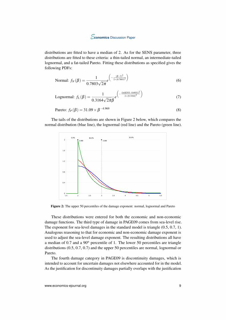
distributions are fitted to have a median of 2. As for the SENS parameter, threedistributions are fitted to these criteria: a thin-tailed normal, an intermediate-tailedlognormal, and a fat-tailed Pareto. Fitting these distributions as specified gives thefollowing PDFs:

Normal: fN (β ) =1

0.7803√

2πe

(− (β−2)2

2×(0.7803)2

)(6)

Lognormal: fL (β ) =1

0.3164√

2πβe

(− (lnSENS−0.6931)2

2×(0.3164)2

)(7)

Pareto: fP (β ) = 31.09×β−4.969 (8)

The tails of the distributions are shown in Figure 2 below, which compares thenormal distribution (blue line), the lognormal (red line) and the Pareto (green line).

3.0002.000

20.0%80.0%0.0%

0

0.4

0.8

1.2

1.6

2

1.5 2 2.5 3 3.5 4 4.5 5 5.5

Figure 2: The upper 50 percentiles of the damage exponent: normal, lognormal and Pareto

These distributions were entered for both the economic and non-economicdamage functions. The third type of damage in PAGE09 comes from sea-level rise.The exponent for sea-level damages in the standard model is triangle (0.5, 0.7, 1).Analogous reasoning to that for economic and non-economic damage exponent isused to adjust the sea-level damage exponent. The resulting distributions all havea median of 0.7 and a 90th percentile of 1. The lower 50 percentiles are triangledistributions (0.5, 0.7, 0.7) and the upper 50 percentiles are normal, lognormal orPareto.

The fourth damage category in PAGE09 is discontinuity damages, which isintended to account for uncertain damages not elsewhere accounted for in the model.As the justification for discontinuity damages partially overlaps with the justification

www.economics-ejournal.org 9

conomics Discussion Paper

for extending the tails on the damage exponents, we have switched them off here tobe sure to avoid double-counting.17

2 Results

The results show significant changes in the estimated value of the SCCO2 whendifferent tails are inputted for the relevant PDFs. Following the steps of our method-ology, the results are presented as follows: (i) the effects of changing the climatesensitivity parameter alone, (ii) the effects of changing the damage functions alone,and (iii) both effects together. For reference, the full set of all results is provided ina single table in the Appendix.

2.1 Climate sensitivity parameter (SENS)

Table 1 shows the results of changing the probability distribution of the climatesensitivity parameter (SENS) only. For comparison, the first column refers tothe standard PAGE09 Model, with the default assumptions. The standard modelprovides a mean value of 102 $/tCO2, which is already higher than many of theestimates in the literature.18

Table 1: Alternative SENS - SCCO2 in US$/tCO2

Standard(triangle)

Thin tail(normal)

Interm. tail(logn.)

Fat tail(Pareto)

Mean 102 131 146 1885th perc. 11 12 11 1250th perc. 49 57 57 5495th perc. 231 374 409 56499th perc. 447 841 1,095 2,797

Source: Authors’ calculations, each based on 10,000 runs of the modified PAGE09.

When the tail for climate sensitivity is normally distributed the SCCO2 meanvalue rises to 131 $/tCO2 (29 percent above the standard model). In the case oflognormal distribution for SENS the mean value is 146 $/tCO2 (44 percent above),while when a Pareto distribution is used the SCCO2 is estimated to be 188 $/tCO2on average (85 percent above).

It is worth emphasising the asymmetry of the effects on the SCCO2 range. Asexpected, the values of the 5th and 50th percentiles do not change significantly, whilethere is a large increase for the 95th and 99th percentiles. Using a normal distributionfor climate sensitivity implies that SCCO2 would be larger than 374 $/tCO2 with a

17 The same is done in Dietz et al. (forthcoming).18 Many of the reasons for this (especially the differences between PAGE2002 and PAGE09) areexplained in Ackerman et al. (2009b) and Hope (2011).

www.economics-ejournal.org 10

conomics Discussion Paper

5 percent probability, and there would be a probability of 1 percent that the value ofSCCO2 is above 841 $/tCO2 (which is 88 percent higher than the 99th percentileof the standard PAGE09 Model). In the case of the Pareto distribution the value ofthe 95th percentile is 564 $/tCO2 and that of the 99th percentile19 is 2,797 $/tCO2,which corresponds to an increase of 144 percent and 525 percent respectively, withrespect to the estimates of the standard PAGE09 Model.

2.2 Damage exponents

Table 2 reports the results of the runs when the distribution of the damage exponentsis modified, without changing the distribution of the sensitivity parameter. In thesecases, as discussed in the previous section, the probability of discontinuity damagesis switched off, to avoid double counting. In order to distinguish which part of thechanges is due to removing the discontinuity damages and which part is due toadding the tails, the standard PAGE09 Model is run with the discontinuity damagesswitched off (second column of Table 2). This alone gives a significantly lowermean value for the SCCO2, equal to 76 $/tCO2.

Table 2: Alternative damage exponents - SCCO2 in US$/tCO2

standard(triangle)

standard(triangle)

Disc. OFF

thin tail(normal)

interm. tail(logn.)

fat tail(Pareto)

Mean 102 76 99 94 1145thperc. 11 11 11 11 11

50th perc. 49 48 50 50 5095th perc. 231 226 300 300 35899th perc. 447 418 658 762 1,421

Source: Authors’ calculations, each based on 10,000 runs of the modified PAGE09.

Modifying the PDFs of the damage exponents raises the SCCO2 (in a similarway as for changing climate sensitivity) relative to the standard model without dis-continuity damages. When comparing to the full standard model (with discontinuitydamages), adding thin, intermediate or fat tails either lowers the mean value of theSCCO2 by 3 or 7 percent or raises it by 12 percent respectively (99, 94 and 114$/tCO2 compared to 102).

19 The 99thpercentile is rarely reported for the estimates of the SCCO2 in the literature. We include ithere because in the context of the discussion about climate uncertainty, we believe it is important toacknowledge the extreme values, even if they are highly unlikely. Roughly speaking extended tailsfor the PDF of the inputs to the model leads to extended tails in the outputs. This is a relevant result,which we wish to show. Nevertheless, it should also be acknowledged that, as one would expect, thevalues for the 99thpercentiles relatively imprecise, varying fairly considerably if the same scenario isrerun.

www.economics-ejournal.org 11

conomics Discussion Paper

2.3 SENS and damage exponents together

Table 3 shows the results of the model when both changes (on SENS and the damageexponents) are done in combination.

Table 3: Alternative SENS and damage exponents - SCCO2 in US$/tCO2

standard(triangle)

thin tail(normal)

interm. tail(logn.)

fat tail(Pareto)

Mean 102 135 147 2185thperc. 11 12 12 11

50th perc. 49 58 57 5595th perc. 231 489 551 83999th perc. 447 1,276 1,660 3,082

Source: Authors’ calculations, each based on 10,000 runs of the modified PAGE09.

The adjusted model, with both SENS and the damage exponents normallydistributed, estimates the average SCCO2 to be 135 $/tCO2 on average, 147 $/tCO2with the lognormal distribution and 216 $/tCO2 with the Pareto distribution. Thenew SCCO2 is 33 to 115 percent higher than the standard PAGE09 Model.

As in the previous cases, the lower half of the distribution is essentially un-changed (adjusting the tail has little impact on the bulk of the results). The upperpercentiles, however, are greatly extended. The 95th percentile shows rises frombetween 110 to 260 percent, while the 99th percentile shows even greater rises. Thereason for this behaviour of the model has partly to do with changes in the way ex-treme damages are modelled. By adding tails, in place of the original discontinuitydamages, the very few, very large "tipping point" damages of the standard modelare removed. In the SCCO2 PAGE09, the marginal change is only responsiblefor a change in discontinuity damage in less than one percent of the runs (when itdoes occur, the impact is very large). Therefore, these very large damages do notinfluence even the 99th percentile in the standard models results.

2.4 Comparison with existing estimates

Many estimates of the SCCO220 have been proposed in the literature.21 Tol (2005)gathered over 100 estimates from 28 published studies and combined them to forma probability density function with a median of 4 $/tCO2, a mean of 25 $/tCO2,

20 Note that many of the results quoted here were originally reported as estimates of the social costof carbon (not of carbon dioxide). These have been converted into SCCO2 units. The multiplier fordoing so is the relative molecular weight of CO2 to carbon, which is 3.67 (44 g per mole/12 g permole;Interagency Working Group on Social Cost of Carbon, U.S. Government (2010)). For example,this means that 100 $/tCO2 is equivalent to 367 $/tC.21 Some early estimates include Frankhauser (1994) that reports marginal impacts of between 2 and12 $/tCO2 with a mean value of 5 $/tCO2 (figures in US$1990). The Second Assessment Report fromthe IPCC (1996) estimates range from 1 to 34 $/tCO2 (US$1990). Tol (1999) estimates the marginalimpact to be between 2 and 6 $/tCO2 (US$1990).

www.economics-ejournal.org 12

conomics Discussion Paper

and a 95thpercentile of 95 $/tCO2. In an updated version of this meta-analysis, Tol(2008) considered 211 estimates of the SCC, including the Stern Review (Stern,2007), and found higher estimates than in the previous studies. Adjusting alternativekernel density estimators to data points, the author found that when the Gaussiandistribution and the sample coefficient of variation is used (which is the case closestto the 2005 study), the distribution of the estimates has a median of 4 $/tCO2, amean of 28 $/tCO2 and a 95th(99th) percentile of 162 $/tCO2 (552 $/tCO2).

A recent report of the US Government Interagency Working Group on SocialCost of Carbon (2010) presents SCCO2 estimates resulting from three IAMs, theDICE, PAGE 2002 and FUND models. The SCCO2 estimates from the average ofthe three IAMs are 35, 21 and 5 $/tCO2, at discount rates of 2.5 percent, 3 percentand 5 percent, respectively.

Our results appear to be significantly higher than the average SCCO2 estimatesprovided in the literature so far. Nevertheless, comparing our results with pastestimates is not straightforward, as differences in the model structure and parametervalues,22 emissions and socioeconomic scenarios and discount factor assumptionsmight bias the effects of introducing uncertainties in key parameters. While we candirectly compare the results of the PAGE09 model before and after fat-tail adjust-ments, further research would be needed to isolate the impact of these adjustmentswith respect to the different models and model assumptions used in previous studies.

3 Conclusions

There are large uncertainties surrounding the catastrophic impacts climate changemight cause. These uncertainties call into question the appropriate weight in the tailsof the probability distributions in climate models. Following recent literature andtaking advantage of the flexible nature of IAMs, we have adjusted the tails of twokey areas of uncertainty in the PAGE09 Model: the climate sensitivity parameterand the damage exponents. For each, we considered a normal (thin), a lognormal(intermediate) and a Pareto (fat) tail. Though there are some doubts about theprobabilities for the bulk of these distributions, we focused on the extreme valueswhich are the most uncertain.

Which of the three tail shapes is the most credible can be debated. Underuncertainty, the Bayesian approach leads one towards the presumption of a fat tail(in the absence of reliable information to the contrary),23 which would suggest abias towards the Pareto tails in this research. However, perhaps the more importantapproach would be to seek to estimate which distribution gives the most plausibleweight for extreme negative events. The importance of the functional forms used forthe tails in this paper is in the weight given to extreme negative events, as opposed to

22 For instance, ceteris paribus the new features of the standard PAGE09 model alone result in at leasta threefold increase of the SCCO2 estimates with respect to the earlier PAGE 2002 model.23 The position is explained in Weitzman (2009).

www.economics-ejournal.org 13

conomics Discussion Paper

the mathematical shape. This type of thinking24 is more relevant whenever damagesare bounded (as they are in IAMs).25

The potential for a change in the tail probabilities to cause up to an approx-imate doubling of the mean value of the SCCO2 and sevenfold increase in the99thpercentile is an important result from our analysis. As constructed here, theeffect of adjusting the climate sensitivity parameter exceeds that of adjusting thedamage function. Not only do both impact on the SCCO2 mean values, but moreespecially on its higher percentiles. It is worth noting the high values for the SCCO2emerging from a minority of runs. For example, our results suggest that it is highlyunlikely that the damage done by emitting a single tonne of CO2 is in excessof a thousand dollars, but the possibility is not vanishingly small. Indeed, if thePareto tails are accepted for both climate sensitivity and the damage exponents, theprobability that the SCCO2 exceeds US$1,000 is 4 percent.

The limitations of IAMs should be taken into account when interpreting theresults. Specifically in relation to the dismal theorem (Weitzman, 2009), the method-ology developed in this paper goes some way towards incorporating uncertaintyinto some key elements of the model, but does not attempt to test the limit of thisparticular critique.26 Furthermore, the impact of the discount rate has not beeninvestigated, and PAGE09 standard values have been used. It is clear from theliterature, and from experimentation with the model, that raising (lowering) the puretime preference time and/or the elasticity of the marginal utility of consumptionwould lower (raise) the SCCO2.

The relationship of the SCCO2 to Pigouvian taxation makes it an importantfigure for policy makers. The weight placed on extreme outcomes for policypurposes depends the level of risk aversion. In fact, as there is uncertainty about thePDF of many parameters, the concept of ambiguity aversion (beyond risk aversion)is also applicable in this context. A higher risk/ambiguity aversion gives moreconsideration to the negative extremes, which leads to the notion of climate policybeing justified, in part, as insurance against catastrophe.

24 This argument is expanded upon in Pindyck (forthcoming).25 It would, of course, have been possible to introduce a thin-tailed distribution that would havecaused higher values for the SCCO2, simply by adjusting the mean and standard deviation (thoughthe justification for doing so would have been somewhat arbitrary).26 Weitzman (forthcoming) emphasizes that the key "fat tail" is that of the PDF of the log of overalldisutility of climate change, resulting from a chain of uncertain, interacting components.

www.economics-ejournal.org 14

conomics Discussion Paper

References

Ackerman, F., De Canio, S. J., Howarth, R. B., and Sheeran, K. (2009a). Limitationsof the integrated assessment models of climate change. Climatic Change, 95: 297–315. URL http://www.springerlink.com/content/c85v5581x7n74571/fulltext.pdf.

Ackerman, F., and Stanton, E. (2010). The social cost of carbon. real-world eco-nomics review, 53: 129–143. URL http://www.paecon.net/PAEReview/issue53/whole53.pdf.

Ackerman, F., Stanton, E., Hope, C., and Alberth, S. (2009b). Did the Stern Reviewunderestimate US and global climate damages? Energy Policy, 37(7): 2717–2721.URL http://www.sciencedirect.com/science/article/pii/S0301421509001529.

Bosello, F., and Roson, R. (2007). Estimating a Climate Change Damage Functionthrough General Equilibrium Modeling. Working Paper Department of EconomicsCa’ Foscari University of Venice, (08/WP/2007). URL http://www.dse.unive.it/fileadmin/templates/dse/wp/WP_2007/WP_DSE_bosello_roson_08_07.pdf.

Dietz, S. (forthcoming). The Treatment of Risk and Uncertainty in the US So-cial Cost of Carbon for Regulatory Impact Analysis. Economics: The Open-Access, Open-Assessment E-Journal. URL http://www.economics-ejournal.org/economics/discussionpapers/2011-30.

Dietz, S., Hope, C., and Patmore, N. (2007). Some economics of "danger-ous" climate change: Reflections on the Stern Review. Global EnvironmentalChange, 17(3-4): 311–325. URL http://www.sciencedirect.com/science/article/pii/S095937800700043X.

Dietz, S., Hope, C., and Patmore, N. (forthcoming). High impact, low probability?An empirical analysis of risk in the economic of climate change. Climatic Change.URL http://www.springerlink.com/content/345l552923k4144w/fulltext.pdf.

European Commission (2007). Communication from the Commission to the Coun-cil, the European Parliament, the European Economic and Social Committee andthe Committee of the Regions. Limiting Global Climate Change to 2 degreesCelsius: The way ahead for 2020 and beyond. URL http://eur-lex.europa.eu/LexUriServ/LexUriServ.do?uri=COM:2007:0002:FIN:EN:PDF.

Frankhauser, S. (1994). The social costs of greenhouse gas emissions: an expectedvalue approach. Energy Journal, 15(2).

Hansen, J., Sato, M., Kharecha, P., Beerling, D., Berner, R., Masson-Delmotte, V.,Pagani, M., Raymo, M., Royer, D., and Zachos, J. (2008). Target atmosphericCO2: Where should humanity aim? Atmospheric and Oceanic Physics, 2: 217–231. URL http://benthamscience.com/open/toascj/articles/V002/217TOASCJ.pdf.

www.economics-ejournal.org 15

conomics Discussion Paper

Hope, C. (2006). The marginal impact of CO2 from PAGE2002: An integratedassessment model incorporating the IPCC’s five reasons for concern. IntegratedAssessment, 6(1): 19–56. URL http://journals.sfu.ca/int_assess/index.php/iaj/article/view/227/190.

Hope, C. (2008). Discount rates, equity weights and the social cost of carbon. En-ergy Economics, 30(3): 1011–1019. URL http://www.sciencedirect.com/science/article/pii/S0140988306001459.

Hope, C. (2011). The PAGE09 integrated assessment model: A technical description.Cambridge Judge Business School Working Paper, 4/11. URL http://www.jbs.cam.ac.uk/research/working_papers/2011/wp1104.pdf.

Hope, C., Anderson, J., and Wenman, P. (1993). Policy analysis of the greenhouseeffect: an application of the PAGE model. Energy Policy, 21(3): 327–338.

Interagency Working Group on Social Cost of Carbon, U.S. Government (2010).Technical Support Document: Social Cost of Carbon for regulatory ImpactAnalysis. Under Executive Order 12866. URL http://www.epa.gov/oms/climate/regulations/scc-tsd.pdf.

IPCC (1996). Climate Change 1995: Impacts, Adaptation and Mitigation ofClimate Change: Scientific-Technical Analysis. Contribution of Working GroupII to the Second Assessment Report of the Intergovernmental Panel on ClimateChange. Cambridge University Press, Cambridge, UK. URL http://www.ipcc.ch/ipccreports/sar/wg_II/ipcc_sar_wg_II_full_report.pdf.

IPCC (2007). Climate Change 2007: Synthesis Report. Contribution of WorkingGroups I, II and III to the Fourth Assessment Report of the IntergovernmentalPanel on Climate Change. URL http://www.ipcc.ch/publications_and_data/ar4/syr/en/contents.html.

Knutti, R., and Hegerl, G. C. (2008). The equilibrium sensitivity of the Earth’stemperature to radiation chages. Nature Geoscience, 1: 735–743. URL http://www.iac.ethz.ch/people/knuttir/papers/knutti08natgeo.pdf.

Kriegler, E., Hall, J., Held, H., Dawson, R., and Schellnhube, H. (2009). ImpreciseProbability Assessment of Tipping Points in the Climate System. Proceedingsof the National Academy of Science of the USA, 106(13): 5041–5046. URL

http://www.pnas.org/content/early/2009/03/13/0809117106.full.pdf.

Lenton, T., Held, H., Kriegler, E., Hall, J., Lucht, W., Rahmstorf, S., and Schellnhu-ber, H. J. (2008). Tipping elements in the Earth’s climate system. Proceedingsof the National Academy of Sciences of the USA, 105(6): 1786–1793. URL

http://www.pnas.org/content/105/6/1786.full.pdf.

Nordhaus, W. (2009). An analysis of the Dismal Theorem. Cowles FoundationDiscussion Paper, 1686. URL http://cowles.econ.yale.edu/P/cd/d16b/d1686.pdf.

www.economics-ejournal.org 16

conomics Discussion Paper

Nordhaus, W., and Boyer, J. (2000). Warming the World: EconomicModels of Global Warming. The MIT Press, Cambridge, Massachusetts,USA. URL http://www.econ.yale.edu/~nordhaus/homepage/web%20table%20of%20contents%20102599.htm.

Patt, A., van Vuuren, D., Berkhout, F., Aaheim, A., Hof, A., Isaac, M., and Mechler,R. (2010). Adaptation in integrated assessment modelling: where do we stand?Climatic Change, 99(3-4): 383–402. URL http://www.springerlink.com/content/q0026gu420415704/fulltext.pdf.

Pindyck, R. (forthcoming). Fat tails, thin tails and climate change policy. Economics:The Open-Access, Open-Assessment E-Journal. URL http://web.mit.edu/rpindyck/www/Papers/FatTailsREEP0910.pdf.

Plambeck, E., Hope, C., and Anderson, J. (1997). The PAGE95 model: Integratingthe science and economics of global warming. Energy Economics, 19(1): 77–101.

Stern, N. (2007). Stern Review on the Economics of Climate Change. HM Treasury,UK. URL http://webarchive.nationalarchives.gov.uk/+/http://www.hm-treasury.gov.uk/stern_review_report.htm.

Tol, R. (1999). The marginal costs of greenhouse gas emissions. The EnergyJournal, 20(1): 61–81.

Tol, R. (2005). The marginal damage costs of carbon dioxide emissions: anassessment of uncertainties. Energy Policy, 33(16): 2064–2074. URL http://www.fnu.zmaw.de/fileadmin/fnu-files/publication/tol/enpolmargcost.pdf.

Tol, R. (2008). The Social Cost of Carbon: Trends, Outliers and Catastrophes.Economics: The Open-Access, Open-Assessment E-Journal, 2(25): 1–22. URL

http://dx.doi.org/10.5018/economics-ejournal.ja.2008-25.

Warren, R., Hope, C., Mastrandrea, M., Tol, R., Adger, N., and Lorenzoni, I.(2006). Spotlighting the Impacts Functions in Integrated Assessment. ResearchReport Prepared for the Stern Review on the Economics of Climate Change.Tyndall Centre for Climate Change Research Working Paper, (91). URL http://www.dfld.de/Presse/PMitt/2006/061030c4.pdf.

Weitzman, M. (2007). A review of the stern review on the economics of climatechange. Journal of Economic Literature, 45(3): 703–724. URL http://ejournals.ebsco.com/direct.asp?ArticleID=475EB1FEC45E5A284E36.

Weitzman, M. (2009). On modelling and interpreting the economics of catastrophicclimate change. The Review of Economics and Statistics, 91(1): 1–19. URL

http://www.mitpressjournals.org/doi/pdfplus/10.1162/rest.91.1.1.

Weitzman, M. (2010). GHG Targets as Insurance Against catastrophic ClimateChange. URL http://www.economics.harvard.edu/faculty/weitzman/files/1A1A.InsuranceCatastrophicRisks.pdf.

www.economics-ejournal.org 17

conomics Discussion Paper

Weitzman, M. (forthcoming). Fat-Tailed Uncertainty in the Economics ofCatastrophic Climate Change. Review of Environmental and Economic Pol-icy. URL http://www.economics.harvard.edu/faculty/weitzman/files/REEP2011%2Bfat-tail.pdf.

Zickfield, K., Morgan, M., Frame, D., and Keith, D. (2010). Expert judgments abouttransient climate response to alternative trajectories of radiative forcing. Proc.of the National Aademy of Sciences of the United States of America, pages 1–6.URL http://www.pnas.org/content/early/2010/06/24/0908906107.full.pdf+html.

www.economics-ejournal.org 18

conomics Discussion Paper

A Full Results Table

Table 4 details all the results for the SCCO2 each based on 10,000 runs. Most ofthese results appear in Tables 1, 2 and 3, which are also accompanied by moredetailed explanations. Here the results are placed all together to allow directcomparisons and also to report three "intermediate" results for SENS with a normal,lognormal and Pareto tail with the discontinuity damages switched off.

Table 4: Full Results Table – SCCO2 in US$/tCO2 each based on 10,000 runs of PAGE09

DAMAGE EXPONENTSdisc. ON discontinuity damages OFFstandard standard normal lognorm. Pareto

SEN

S

stan

dard

Mean 102 76 99 94 1145thperc. 11 11 11 11 1150thperc. 49 48 50 50 5095thperc. 231 226 300 300 35899thperc. 447 418 658 762 1,421

norm

al

Mean 131 107 1355thperc. 12 12 1250thperc. 57 57 5895thperc. 374 374 48999thperc. 841 744 1,276

logn

orm

al

Mean 146 120 1475thperc. 11 11 1250thperc. 57 56 5795thperc. 409 412 55199thperc. 1,095 1,045 1,660

Pare

to

Mean 188 162 2185thperc. 12 12 1150thperc. 54 53 5595thperc. 564 549 83999thperc. 2,797 1,996 3,082Source: Authors’ calculations, each based on 10,000 runs of the modified PAGE09.

www.economics-ejournal.org 19

Please note:

You are most sincerely encouraged to participate in the open assessment of this discussion paper. You can do so by either recommending the paper or by posting your comments.

Please go to:

http://www.economics-ejournal.org/economics/discussionpapers/2011-36

The Editor

© Author(s) 2011. Licensed under a Creative Commons License - Attribution-NonCommercial 2.0 Germany