Sensors 2013, 13, 4029-4040; doi:10.3390/s130404029

sensors ISSN 1424-8220

www.mdpi.com/journal/sensors

Article

A Support-Based Reconstruction for SENSE MRI

Yudong Zhang, Bradley Peterson and Zhengchao Dong *

Brain Imaging Lab & MRI Unit, New York State Psychiatry Institute & Columbia University,

New York, NY 10032, USA; E-Mails: petersob@nyspi.columbia.edu (B.P.);

dongzh@nyspi.columbia.edu (Z.D.)

* Author to whom correspondence should be addressed; E-Mail: dongzh@nyspi.columbia.edu.

Received: 1 March 2013; in revised form: 22 March 2013 / Accepted: 22 March 2013 /

Published: 25 March 2013

Abstract: A novel, rapid algorithm to speed up and improve the reconstruction of

sensitivity encoding (SENSE) MRI was proposed in this paper. The essence of the

algorithm was that it iteratively solved the model of simple SENSE on a pixel-by-pixel

basis in the region of support (ROS). The ROS was obtained from scout images of eight

channels by morphological operations such as opening and filling. All the pixels in the

FOV were paired and classified into four types, according to their spatial locations with

respect to the ROS, and each with corresponding procedures of solving the inverse problem

for image reconstruction. The sensitivity maps, used for the image reconstruction and

covering only the ROS, were obtained by a polynomial regression model without

extrapolation to keep the estimation errors small. The experiments demonstrate that the

proposed method improves the reconstruction of SENSE in terms of speed and accuracy.

The mean square errors (MSE) of our reconstruction is reduced by 16.05% for a 2D brain

MR image and the mean MSE over the whole slices in a 3D brain MRI is reduced by

30.44% compared to those of the traditional methods. The computation time is only 25%,

45%, and 70% of the traditional method for images with numbers of pixels in the orders of

103, 10

4, and 10

5–10

7, respectively.

Keywords: parallel imaging; sensitivity encoding; magnetic resonance imaging; region of

support; sensitivity maps; polynomial model; morphological operator

OPEN ACCESS

Sensors 2013, 13 4030

1. Introduction

Parallel imaging (PI) is one of the most important applications of the phased-array surface coils

introduced to the field of MRI more than two decades ago [1]. PI makes use of the characteristic

sensitivity distributions of the spatially separated receiver coils to provide an additional spatial

encoding mechanism, in addition to the conventional phase encoding and frequency encoding required

for MRI. This sensitivity-based encoding allows one to skip some phase encoding steps, speeding up

the acquisition of the MRI data. Several PI methods have been proposed in the past decade, and they

can be classified into two main types according to the working domains for the image reconstruction [2].

One is the k-space-based method, such as simultaneous acquisition of spatial harmonics (SMASH) and

generalized autocalibrating partially parallel acquisitions (GRAPPA) [3], in which the missing phase

encoding data points in k-space were synthesized by combining the sensitivity information of the coils

and the acquired phase encoding and frequency encoding data [4]; The other is the image domain-based

method, such as sensitivity encoding (SENSE) [5], in which the full image was recovered from the

sensitivity maps, derived from scout images acquired during the patient setup, and the folded images

reconstructed directly from the undersampled data of the individual coil components. In this paper, we

focus our research on the latter, which is most widely used in clinical practice, and propose a rapid and

accurate algorithm for the reconstruction of SENSE MRI.

Consider a simple 2D SENSE with an acceleration rate of r, in which every (r−1) phase encoding

lines in the conventional fully sampled k-space were skipped [6]. According to the Nyquist theorem,

the resultant images of the component coils would be folded in the dimension corresponding to the

phase encoding direction. The basic principle of the SENSE technique is to unfold the images with the

help of the sensitivity maps to recover the full images. The data acquired at m image points by an array

of c coils can be expressed in the form of direct problem as a set of linear equations:

(1)

where S is an mc × n sensitivity map, ρ is an n × 1 column vector denoting the desired full image, and

b is an mc × 1 column vector whose elements are points in the folded images of the c coils. The

reconstructed full image ρ can be obtained as an inverse problem by solving the above linear equations.

The traditional method for solving Equation (1) suffers from the following three shortcomings [7,8]:

(i) The values of both m and n are of the order of 105, making the computation time of direct image

reconstruction impractically long in clinical settings; (ii) It solved the equations for the entire FOV and

did not take into account the region of support [9]; (iii) The estimation of the sensitivity map is

vulnerable to noises, because it involves extrapolation from the brain area to the background area.

An iterative method was introduced recently for the fast reconstruction of the SENSE-based

MRI [10]. This method significantly reduced computation time and memory storage. However, in this

and previous techniques [11,12], the sensitivity maps were estimated for the full FOV and the

algorithms of reconstruction were also based on the full FOV, without distinguishing regions in the

brain and regions in the background. In fact, the background region often constitutes a significant

portion of the FOV and is filled with noise. Therefore, the signals in the background should be taken as

zeros as prior knowledge and further excluded from the image reconstruction for the benefits of both

accuracy and speed. In this paper we proposed a method for accurate and rapid reconstruction of

S b

Sensors 2013, 13 4031

SENSE MRI. The method is based on the pixel-by-pixel algorithm for the simple SENSE model, and

is applied on the ROS that is obtained by morphological operations such as opening and filling.

Accordingly, the sensitivity map is estimated for the ROS without extrapolation to the whole FOV,

thus avoiding considerable estimation errors. Finally, the method uses the ROS at the reconstruction

stage to guide the equation solving procedures, and uses the accurate sensitivity maps to reconstruct

the full image.

2. Method

2.1. The Simple SENSE Model

For the model of simple 2D SENSE with an acceleration factor r, the k-space data were regularly

undersampled by skipping every r−1 phase encoding lines in the full k-space [13]. Without losing

generality, we consider as an example the case of acceleration factor of r = 2 and the number of coils

c = 8. For a pixel at location (x, y) in the aliased image, the signals measured by each of the eight coils

are given by following equations:

(2)

This is a simplified version of the direct problem previously given in Equation (1), which states that

the signals at the locations of the two pixels (x, y) and (x+FOV/2, y) are aliased to generate the

measured signals in the component coils. The illustration of SENSE is shown pictorially in Figure 1.

2.2. Iterative Method

There are three approaches to SENSE reconstruction [5]: (i) solving Equation (1) directly, which

would take enormous storage and time; (ii) line-by-line iterations, in which each iteration estimates

two rows of the original image; (iii) pixel-by-pixel iterations, recovering two pixels of the original

image in each iteration.

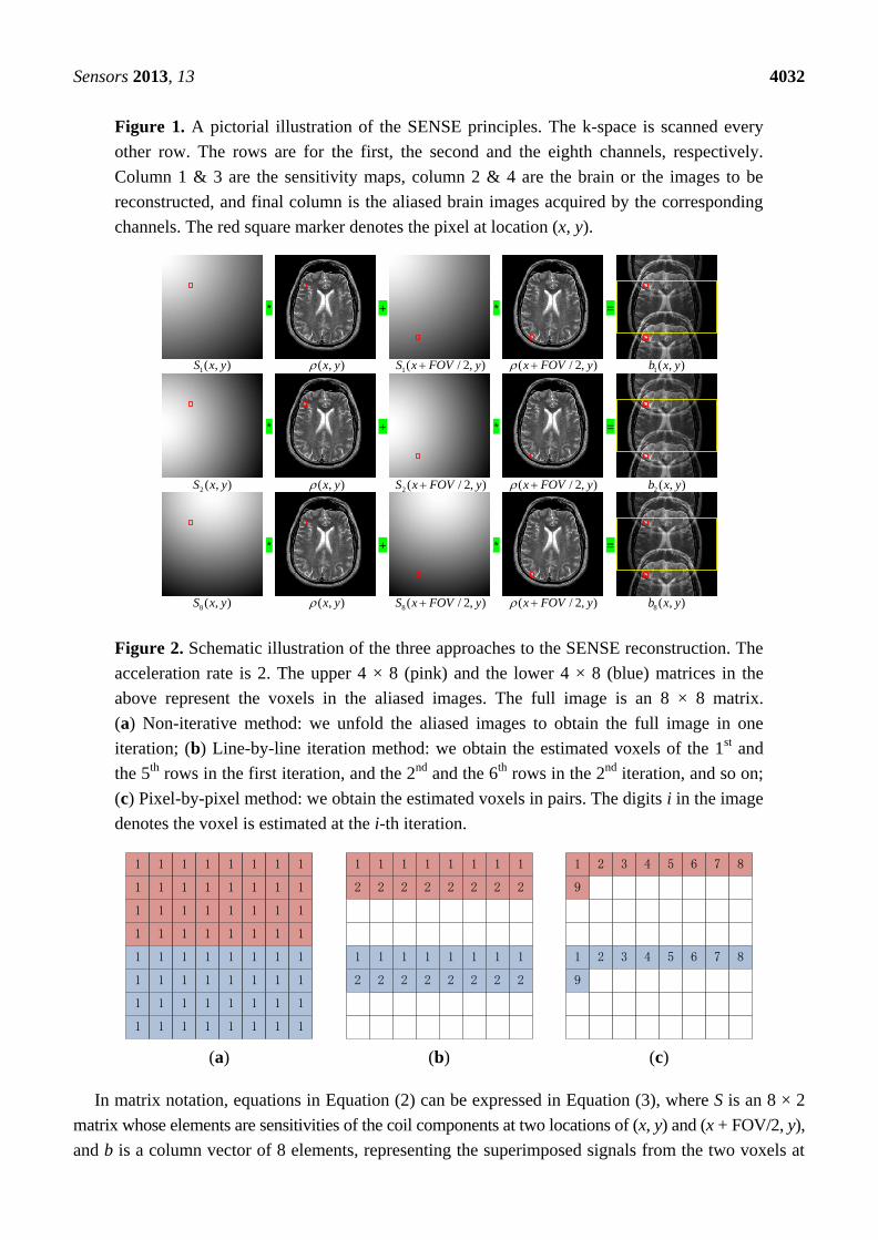
We briefly analyze the three approaches to recovering an 8 × 8 matrix from two aliased 4 × 8

images acquired with an acceleration factor of 2 (Figure 2). The first approach is non-iterative, and we

obtain the estimate of the whole image without iteration. With the line-by-line iteration, we unfold the

first lines in the aliased images to obtain the first and fifth row of the full image at the 1st iteration, and

then we unfold the second lines in the aliased images to obtain the second and sixth row at the 2nd

iteration, and so on. With the pixel-by-pixel iteration, we obtain the ρ(1, 1) and ρ(5, 1) at the 1st

iteration, the ρ(1, 2) and ρ(5, 2) at the 2nd

iteration, until the ρ(1, 8) and ρ(5, 8) at the 8th

iteration; Then

the scan turns to the next row, and we obtain the ρ(2, 1) and ρ(6, 1) at the 9th

iteration, and so on. In

this paper, we chose the pixel-by-pixel iteration since it only requires least memory.

1 1 1

8 8 8

( , ) ( , ) ( , ) ( , ) ( , )2 2

...

( , ) ( , ) ( , ) ( , ) ( , )2 2

FOV FOVS x y x y S x y x y b x y

FOV FOVS x y x y S x y x y b x y

Sensors 2013, 13 4032

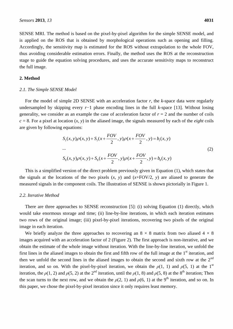
Figure 1. A pictorial illustration of the SENSE principles. The k-space is scanned every

other row. The rows are for the first, the second and the eighth channels, respectively.

Column 1 & 3 are the sensitivity maps, column 2 & 4 are the brain or the images to be

reconstructed, and final column is the aliased brain images acquired by the corresponding

channels. The red square marker denotes the pixel at location (x, y).

Figure 2. Schematic illustration of the three approaches to the SENSE reconstruction. The

acceleration rate is 2. The upper 4 × 8 (pink) and the lower 4 × 8 (blue) matrices in the

above represent the voxels in the aliased images. The full image is an 8 × 8 matrix.

(a) Non-iterative method: we unfold the aliased images to obtain the full image in one

iteration; (b) Line-by-line iteration method: we obtain the estimated voxels of the 1st and

the 5th

rows in the first iteration, and the 2nd

and the 6th

rows in the 2nd

iteration, and so on;

(c) Pixel-by-pixel method: we obtain the estimated voxels in pairs. The digits i in the image

denotes the voxel is estimated at the i-th iteration.

(a) (b) (c)

In matrix notation, equations in Equation (2) can be expressed in Equation (3), where S is an 8 × 2

matrix whose elements are sensitivities of the coil components at two locations of (x, y) and (x + FOV/2, y),

and b is a column vector of 8 elements, representing the superimposed signals from the two voxels at

* + * =

* + * =

* + * =

1( , )S x y

2 ( , )S x y

8 ( , )S x y

( , )x y

( , )x y

( , )x y

1( / 2, )S x FOV y

2 ( / 2, )S x FOV y

8 ( / 2, )S x FOV y

( / 2, )x FOV y

( / 2, )x FOV y

( / 2, )x FOV y

1( , )b x y

2 ( , )b x y

8 ( , )b x y

1 1 1 1 1 1 1 1

1 1 1 1 1 1 1 1

1 1 1 1 1 1 1 1

1 1 1 1 1 1 1 1

1 1 1 1 1 1 1 1

1 1 1 1 1 1 1 1

1 1 1 1 1 1 1 1

1 1 1 1 1 1 1 1

1 1

2

1 1 1 1 1 1

1 1

2

1 1 1 1 1 1

2 2 2 2 2 2 2

2 2 2 2 2 2 2

1 2

9

3 4 5 6 7 8

1 2

9

3 4 5 6 7 8

Sensors 2013, 13 4033

(x, y) and (x+FOV/2, y) recorded by the eight coil components. The two intensities of ρ(x, y) and

ρ(x+FOV/2, y) were obtained by solving the following equations:

(3)

Here S1 and S

2 are two column vectors of eight elements. In essence, the solution of Equation (3) is

a procedure of recovering the two voxels at (x, y) and (x+FOV/2, y), by unfolding the superimposed

signals. We will show that the entire image can be reconstructed when all the superimposed signals

within the region of support (ROS) are unfolded. In the following subsections we introduce the

ROS, give the detailed procedures for estimating sensitivity map S based on ROS, and describe the

ROS-based SENSE reconstruction.

2.3. Region of Support

The ROS is detected from the scout images of eight channels [14] (Figure 3). Let Oi denotes the

scout image of the ith channel, the ROS is calculated from following procedures.

(1) Calculate the power image defined as:

(4)

(2) Find the support area. Here we choose the threshold as the 1% of maximum intensity value:

(5)

(3) Perform the opening operation to eliminate the noise artifacts:

(6)

(4) Use the filling method of mathematical morphologic operations to fill the holes:

(7)

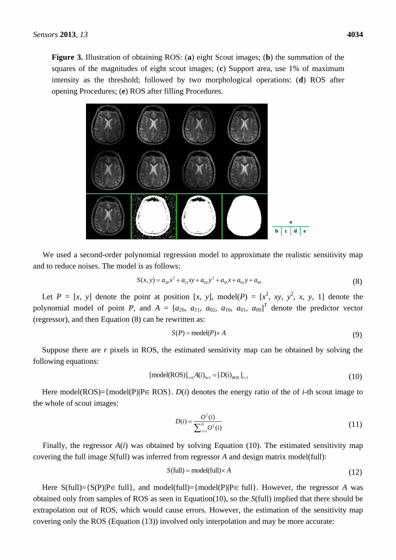
The mean essence of the algorithm is thresholding based on the signal-to-noise ratio (SNR),

because the brain area usually contains higher signal than the background does. But other

morphological operations are also necessary to ensure an example of these procedures is illustrated in

Figure 3. The final extracted ROS was very close to the shape of the brain.

2.4. Estimation of Sensitivity Maps

In the literature [9,10], sensitivity maps were generated for the whole FOV by fitting and

extrapolating the raw sensitivity maps obtained from low resolution scout images acquired in a fast

reference scan. Sensitivity maps in the whole FOV facilitate the whole FOV-based reconstruction of

SENSE MRI, but they are difficult to estimate accurately not only in the background region but

also within the brain, because the extrapolation inevitably introduces errors. We therefore adopted an

ROS-based approach to accurately estimating sensitivity maps.

8 2 8 1

1 2

8 2 8 1 8 1

( , )

( , )2

x y

S bFOVx y

S S S

82

1

i

i

E O

1 0.01 max( )T E E

2 1open( )T T

2fill( )ROS T

Sensors 2013, 13 4034

Figure 3. Illustration of obtaining ROS: (a) eight Scout images; (b) the summation of the

squares of the magnitudes of eight scout images; (c) Support area, use 1% of maximum

intensity as the threshold; followed by two morphological operations: (d) ROS after

opening Procedures; (e) ROS after filling Procedures.

We used a second-order polynomial regression model to approximate the realistic sensitivity map

and to reduce noises. The model is as follows:

(8)

Let P = [x, y] denote the point at position [x, y], model(P) = [x2, xy, y

2, x, y, 1] denote the

polynomial model of point P, and A = [a20, a11, a02, a10, a01, a00]T denote the predictor vector

(regressor), and then Equation (8) can be rewritten as:

(9)

Suppose there are r pixels in ROS, the estimated sensitivity map can be obtained by solving the

following equations:

(10)

Here model(ROS)={model(P)|PROS}. D(i) denotes the energy ratio of the of i-th scout image to

the whole of scout images:

(11)

Finally, the regressor A(i) was obtained by solving Equation (10). The estimated sensitivity map

covering the full image S(full) was inferred from regressor A and design matrix model(full):

(12)

Here S(full)={S(P)|Pfull}, and model(full)={model(P)|Pfull}. However, the regressor A was

obtained only from samples of ROS as seen in Equation(10), so the S(full) implied that there should be

extrapolation out of ROS, which would cause errors. However, the estimation of the sensitivity map

covering only the ROS (Equation (13)) involved only interpolation and may be more accurate:

a

b c d e

2 2

20 11 02 10 01 00( , )S x y a x a xy a y a x a y a

( ) model( )S P P A

6 6 1 1[model(ROS)] ( ) [ ( ) ]r ROS rA i D i

2

8 2

1

( )( )

( )i

O iD i

O i

(full) model(full)S A

Sensors 2013, 13 4035

(13)

Here S(ROS)={S(P)|PROS}. An example of the estimation of sensitivity maps is illustrated in

Figure 4.

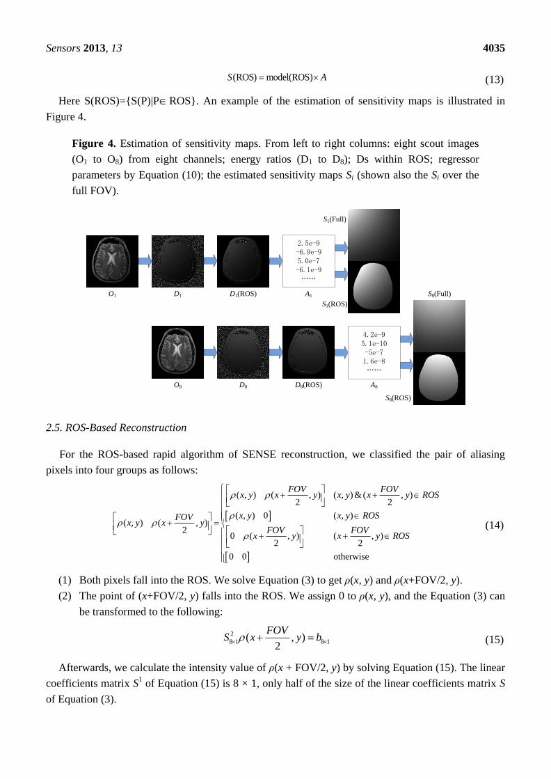
Figure 4. Estimation of sensitivity maps. From left to right columns: eight scout images

(O1 to O8) from eight channels; energy ratios (D1 to D8); Ds within ROS; regressor

parameters by Equation (10); the estimated sensitivity maps Si (shown also the Si over the

full FOV).

2.5. ROS-Based Reconstruction

For the ROS-based rapid algorithm of SENSE reconstruction, we classified the pair of aliasing

pixels into four groups as follows:

( , ) ( , ) ( , ) & ( , )2 2

( , ) 0 ( , )( , ) ( , )

20 ( , ) ( , )

2 2

0 0 otherwise

FOV FOVx y x y x y x y ROS

x y x y ROSFOVx y x y

FOV FOVx y x y ROS

(14)

(1) Both pixels fall into the ROS. We solve Equation (3) to get ρ(x, y) and ρ(x+FOV/2, y).

(2) The point of (x+FOV/2, y) falls into the ROS. We assign 0 to ρ(x, y), and the Equation (3) can

be transformed to the following:

(15)

Afterwards, we calculate the intensity value of ρ(x + FOV/2, y) by solving Equation (15). The linear

coefficients matrix S1 of Equation (15) is 8 × 1, only half of the size of the linear coefficients matrix S

of Equation (3).

(ROS) model(ROS)S A

O1 D1

S1(Full)

S1(ROS)

O8 D8

S8(Full)

S8(ROS)

D1(ROS)

2.5e-9-6.9e-95.0e-7-6.1e-9……

A1

D8(ROS)

4.2e-95.1e-10-5e-71.6e-8……

A8

2

8 1 8 1( , )2

FOVS x y b

Sensors 2013, 13 4036

(3) The point of (x, y) falls into the ROS. Similarly, we assign 0 to ρ(x + FOV/2, y) and transform

Equation (3) to the following,

(16)

Afterwards, we solve Equation (16) to get the intensity value of pixel ρ(x, y).

(4) Neither of the pair falls into the ROS. We assign a value of 0 to each of the pixels. As seen

from Equations (14)–(16), recovering the pixels of groups 1 to 3 is straightforward and only

requires simple arithmetic operations. Only the recovery of pixels of group 4 needs matrix

operation as in the traditional methods. Therefore, our proposed method is computationally

simple and can be executed rapidly.

3. Experiments

We carried out experiments to assess the performance of our method and, in particular, to compare

our method with the traditional methods. The experiments were carried out on the platform of

Windows XP on a desktop PC rquipped with an Intel Pentium 4, 3 GHz processor and 2 GB memory.

The programs were developed via Matlab 2010b.

3.1. Comparison of the Algorithms

The traditional method used ROS as a correction tool, viz., to multiply final reconstruction results

with the ROS to reduce the background noises. We call it “ROS-based correction” for short. In our

method, we used the ROS at the reconstruction stage to group the pairs into different types, which is

referred to as “ROS-based reconstruction”. The main differences of ROS-based correction and

ROS-based reconstruction lie in the following three points (shown in the red font in Figure 5):

(1) ROS-based correction calculates the sensitivity map of the full image, which involves

extrapolation; however, ROS-based reconstruction only needs the sensitivity map within the

ROS, which only involves interpolation.

(2) ROS-based correction directly solves Equation (3) no matter the pixel pairs locate in the ROS

or in the background. Conversely, the ROS-based reconstruction classifies Equation (3) into

four types, and solves different type by different methods, which greatly hasten the procedures.

(3) ROS-based correction needs to correct the final result by multiplying it with the ROS, while the

ROS-based reconstruction is free from this procedure.

3.2. The Quality of the Reconstruction

We compared our proposed ROS-based reconstruction method with traditional ROS-based

correction method. We first used a fully sampled T2 weighted brain MRI image as a reference data set,

undersampled the data with an acceleration rate of 2, applied the aforementioned two methods to

reconstruct the images from the undersampled data, and compared the results of the two methods using

mean absolute error (MAE) and mean square errors (MSE), which were calculated against the ground

truth. To facilitate fair comparison, we calculated MAEs and MSEs on the ROS instead of the whole

FOV. In order to assess the performance of sensitivity map estimation, we added Gaussian noise of

1

8 1 8 1( , )S x y b

Sensors 2013, 13 4037

zero mean and 10−4

variance, which indicates the pixels in the image will have a fluctuation of

256 × = ±2.56 in their gray intensity values.

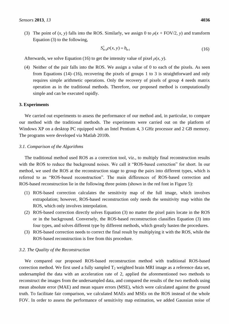
Figure 5. Flowchart of (a) ROS-based correction; (b) ROS-based reconstruction

(the differences are labeled with red color), please see the paragraph below for the details.

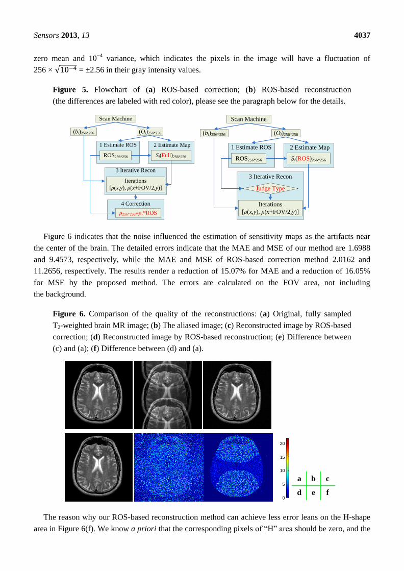
Figure 6 indicates that the noise influenced the estimation of sensitivity maps as the artifacts near

the center of the brain. The detailed errors indicate that the MAE and MSE of our method are 1.6988

and 9.4573, respectively, while the MAE and MSE of ROS-based correction method 2.0162 and

11.2656, respectively. The results render a reduction of 15.07% for MAE and a reduction of 16.05%

for MSE by the proposed method. The errors are calculated on the FOV area, not including

the background.

Figure 6. Comparison of the quality of the reconstructions: (a) Original, fully sampled

T2-weighted brain MR image; (b) The aliased image; (c) Reconstructed image by ROS-based

correction; (d) Reconstructed image by ROS-based reconstruction; (e) Difference between

(c) and (a); (f) Difference between (d) and (a).

The reason why our ROS-based reconstruction method can achieve less error leans on the H-shape

area in Figure 6(f). We know a priori that the corresponding pixels of “H” area should be zero, and the

3 Iterative Recon

4 Correction

Scan Machine

(bi)256*256

1 Estimate ROS

ROS256*256

2 Estimate Map

Si(Full)256*256

(Oi)256*256

Iterations

[ρ(x,y), ρ(x+FOV/2,y)]

ρ256*256=ρ.*ROS

3 Iterative Recon

Scan Machine

(bi)256*256

1 Estimate ROS

ROS256*256

2 Estimate Map

Si(ROS)256*256

(Oi)256*256

Iterations

[ρ(x,y), ρ(x+FOV/2,y)]

Judge Type

0

5

10

15

20

a b c

d e f

Sensors 2013, 13 4038

pixels are recovered in pairs. Therefore, we can get a higher signal-to-noise ratio on the H-shape area

due to the a priori information.

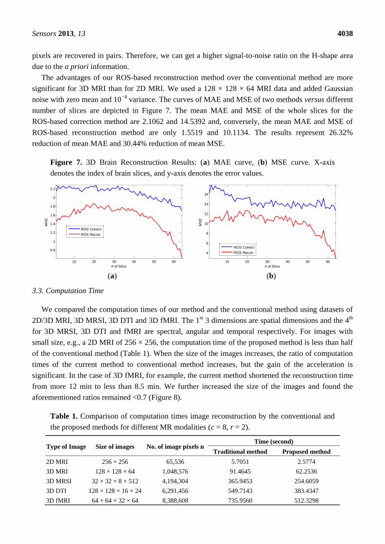
The advantages of our ROS-based reconstruction method over the conventional method are more

significant for 3D MRI than for 2D MRI. We used a 128 × 128 × 64 MRI data and added Gaussian

noise with zero mean and 10−4

variance. The curves of MAE and MSE of two methods versus different

number of slices are depicted in Figure 7. The mean MAE and MSE of the whole slices for the

ROS-based correction method are 2.1062 and 14.5392 and, conversely, the mean MAE and MSE of

ROS-based reconstruction method are only 1.5519 and 10.1134. The results represent 26.32%

reduction of mean MAE and 30.44% reduction of mean MSE.

Figure 7. 3D Brain Reconstruction Results: (a) MAE curve, (b) MSE curve. X-axis

denotes the index of brain slices, and y-axis denotes the error values.

(a)

(b)

3.3. Computation Time

We compared the computation times of our method and the conventional method using datasets of

2D/3D MRI, 3D MRSI, 3D DTI and 3D fMRI. The 1st 3 dimensions are spatial dimensions and the 4

th

for 3D MRSI, 3D DTI and fMRI are spectral, angular and temporal respectively. For images with

small size, e.g., a 2D MRI of 256 × 256, the computation time of the proposed method is less than half

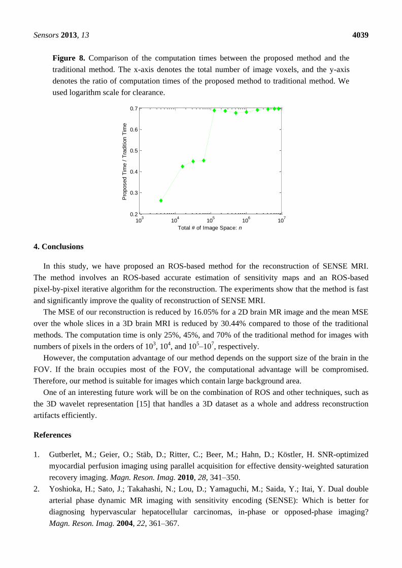
of the conventional method (Table 1). When the size of the images increases, the ratio of computation

times of the current method to conventional method increases, but the gain of the acceleration is

significant. In the case of 3D fMRI, for example, the current method shortened the reconstruction time

from more 12 min to less than 8.5 min. We further increased the size of the images and found the

aforementioned ratios remained <0.7 (Figure 8).

Table 1. Comparison of computation times image reconstruction by the conventional and

the proposed methods for different MR modalities (c = 8, r = 2).

Type of Image Size of images No. of image pixels n Time (second)

Traditional method Proposed method

2D MRI 256 × 256 65,536 5.7051 2.5774

3D MRI 128 × 128 × 64 1,048,576 91.4645 62.2536

3D MRSI 32 × 32 × 8 × 512 4,194,304 365.9453 254.6059

3D DTI 128 × 128 × 16 × 24 6,291,456 549.7143 383.4347

3D fMRI 64 × 64 × 32 × 64 8,388,608 735.9560 512.3298

10 20 30 40 50 60

0.8

1

1.2

1.4

1.6

1.8

2

2.2

# of Slice

MA

E

ROS Correct

ROS Recon

10 20 30 40 50 60

4

6

8

10

12

14

16

# of Slice

MS

E

ROS Correct

ROS Recon

Sensors 2013, 13 4039

Figure 8. Comparison of the computation times between the proposed method and the

traditional method. The x-axis denotes the total number of image voxels, and the y-axis

denotes the ratio of computation times of the proposed method to traditional method. We

used logarithm scale for clearance.

4. Conclusions

In this study, we have proposed an ROS-based method for the reconstruction of SENSE MRI.

The method involves an ROS-based accurate estimation of sensitivity maps and an ROS-based

pixel-by-pixel iterative algorithm for the reconstruction. The experiments show that the method is fast

and significantly improve the quality of reconstruction of SENSE MRI.

The MSE of our reconstruction is reduced by 16.05% for a 2D brain MR image and the mean MSE

over the whole slices in a 3D brain MRI is reduced by 30.44% compared to those of the traditional

methods. The computation time is only 25%, 45%, and 70% of the traditional method for images with

numbers of pixels in the orders of 103, 10

4, and 10

5–10

7, respectively.

However, the computation advantage of our method depends on the support size of the brain in the

FOV. If the brain occupies most of the FOV, the computational advantage will be compromised.

Therefore, our method is suitable for images which contain large background area.

One of an interesting future work will be on the combination of ROS and other techniques, such as

the 3D wavelet representation [15] that handles a 3D dataset as a whole and address reconstruction

artifacts efficiently.

References

1. Gutberlet, M.; Geier, O.; Stäb, D.; Ritter, C.; Beer, M.; Hahn, D.; Köstler, H. SNR-optimized

myocardial perfusion imaging using parallel acquisition for effective density-weighted saturation

recovery imaging. Magn. Reson. Imag. 2010, 28, 341–350.

2. Yoshioka, H.; Sato, J.; Takahashi, N.; Lou, D.; Yamaguchi, M.; Saida, Y.; Itai, Y. Dual double

arterial phase dynamic MR imaging with sensitivity encoding (SENSE): Which is better for

diagnosing hypervascular hepatocellular carcinomas, in-phase or opposed-phase imaging?

Magn. Reson. Imag. 2004, 22, 361–367.

103

104

105

106

107

0.2

0.3

0.4

0.5

0.6

0.7

Total # of Image Space: n

Pro

posed T

ime /

Tra

ditio

n T

ime

Sensors 2013, 13 4040

3. Griswold, M.A.; Jakob, P.M.; Heidemann, R.M.; Nittka, M.; Jellus, V.; Wang, J.; Kiefer, B.;

Haase, A. Generalized autocalibrating partially parallel acquisitions (GRAPPA). Magn. Reson. Med.

2002, 47, 1202–1210.

4. Sodickson, D.K.; McKenzie, C.A.; Ohliger, M.A.; Yeh, E.N.; Price, M.D. Recent advances in

image reconstruction, coil sensitivity calibration, and coil array design for SMASH and

generalized parallel MRI. Magn. Reson. Mat. Biol. Phys. Med. 2002, 13, 158–163.

5. Weiger, M.; Pruessmann, K.P.; Boesiger, P. 2D SENSE for faster 3D MRI. Magn. Reson. Mat.

Biol. Phys. Med. 2002, 14, 10–19.

6. Liang, D.; Liu, B.; Ying, L. Accelerating Sensitivity Encoding Using Compressed Sensing. In

Proceedings of EMBS 2008: 30th IEEE Annual International Conference of the Engineering in

Medicine and Biology Society, Vancouver, BC, Canada, 20–25 August 2008; pp. 1667–1670.

7. Ramani, S.; Fessler, J. Parallel MR image reconstruction using augmented Lagrangian methods.

IEEE Trans. Med. Imag. 2011, 30, 694–706.

8. Allison, M.J.; Ramani, S.; Fessler, J.A. Regularized MR Coil Sensitivity Estimation Using

Augmented Lagrangian Methods. In Proceedings of 9th IEEE International Symposium on

Biomedical Imaging (ISBI), Barcelona, Spain, 2–5 May 2012; pp. 394–397.

9. Zotev, V.S.; Volegov, P.L.; Matlashov, A.N.; Espy, M.A.; Mosher, J.C.; Kraus, R.H., Jr.

Parallel MRI at microtesla fields. J. Magn. Reson. 2008, 192, 197–208.

10. Chaâri, L.; Pesquet, J.-C.; Benazza-Benyahia, A.; Ciuciu, P. A wavelet-based regularized

reconstruction algorithm for SENSE parallel MRI with applications to neuroimaging. Med. Image

Anal. 2011, 15, 185–201.

11. Qu, P.; Luo, J.; Zhang, B.; Wang, J.; Shen, G.X. An improved iterative SENSE reconstruction

method. Concept. Magn. Reson. Part B: Magn. Reson. Eng. 2007, 31B, 44–50.

12. Omer, H.; Dickinson, R. A graphical generalized implementation of SENSE reconstruction using

Matlab. Concept. Magn. Reson. Part A 2010, 36A, 178–186.

13. Bydder, M.; Perthen, J.E.; Du, J. Optimization of sensitivity encoding with arbitrary k-space

trajectories. Magn. Reson. Imag. 2007, 25, 1123–1129.

14. Mislow, J.M.K.; Golby, A.J.; Black, P.M. Origins of Intraoperative MRI. Magn. Reson. Imag.

Clin. N. Am. 2010, 18, 1–10.

15. Chaari, L.; Mériaux, S.; Badillo, S.; Pesquet, J.; Ciuciu, P. Multidimensional Wavelet-Based

Regularized Reconstruction for Parallel Acquisition in Neuroimaging. Available online:

http://arxiv.org/abs/1201.0022 (accessed on 22 March 2013).

© 2013 by the authors; licensee MDPI, Basel, Switzerland. This article is an open access article

distributed under the terms and conditions of the Creative Commons Attribution license

(http://creativecommons.org/licenses/by/3.0/).